A Stochastic Projection Method for Fluid Flow - Olivier Le Maître

Journal of Computational Physics 181, 9–44 (2002)doi:10.1006/jcph.2002.7104

A Stochastic Projection Method for Fluid Flow

II. Random Process

Olivier P. Le Maıtre,∗ Matthew T. Reagan,† Habib N. Najm,†Roger G. Ghanem,‡ and Omar M. Knio§,1

∗Centre d’Etudes de Mecanique d’Ile de France, Universite d’Evry Val d’Essone, 40 rue du Pelvoux, 91020Evry cedex, France; †Combustion Research Facility, Sandia National Laboratories, Livermore,

California 94550; ‡Department of Civil Engineering, The Johns Hopkins University,Baltimore, Maryland 21218-2686; and §Department of Mechanical Engineering,

The Johns Hopkins University, Baltimore, Maryland 21218-2686E-mail: [email protected], [email protected], [email protected],

[email protected], and [email protected]

Received October 1, 2001; revised May 1, 2002

An uncertainty quantification scheme is developed for the simulation of stochasticthermofluid processes. The scheme relies on spectral representation of uncertaintyusing the polynomial chaos (PC) system. The solver combines a Galerkin procedurefor the determination of PC coefficients with a projection method for efficiently sim-ulating the resulting system of coupled transport equations. Implementation of thenumerical scheme is illustrated through simulations of natural convection in a 2Dsquare cavity with stochastic temperature distribution at the cold wall. The propertiesof the uncertainty representation scheme are analyzed, and the predictions are con-trasted with results obtained using a Monte Carlo approach. c© 2002 Elsevier Science (USA)

Key Words: stochastic; natural convection; Navier-Stokes; polynomial chaos;Karhunen–Loeve; uncertainty.

1. INTRODUCTION

Uncertainty propagation and quantification can be an essential step in the developmentof complex models, in particular when these models involve inexact knowledge of sys-tem forcing or system parameters. This article is part of an effort that aims at developinguncertainty quantification schemes for fluid systems involving transport and chemistry.

As an initial step toward these objectives, a stochastic projection method (SPM) was devel-oped in a previous work [1]. In [1] attention was focused on an incompressible flow model,

1 Corresponding author.

9

0021-9991/02 $35.00c© 2002 Elsevier Science (USA)

All rights reserved.

10 LE MAITRE ET AL.

where uncertain model data are generated by a single random variable. SPM combines aprojection method for fluid flow with a spectral representation of the effect of uncertaintyin terms of the polynomial chaos (PC) system [2–9]. The objectives of the present effortare twofold: (1) to extend the capabilities of SPM to situations involving random processes,and (2) to generalize the underlying formulation so as to account for weak compressibilityeffects. To illustrate the development, we focus on natural convection in an enclosed cavity.This topic has received considerable attention in the recent literature and various approacheshave been proposed, including models based on the well-known Boussinesq approximation(e.g., [10–12]) as well as low-Mach-number models (e.g., [13, 14]). In addition, simulationsof internal natural convection have been used as benchmark tests for different flow regimes[10, 15–27].

In one of its simplest forms, the problem consists of a square or rectangular cavity withadiabatic horizontal boundaries and differentially but uniformly heated vertical walls. Inpractice, however, this idealized situation may be difficult to achieve, for instance due toimperfections in insulation and/or nonuniform heating and cooling. Computed solutionsare often very sensitive to applied boundary conditions, which can complicate comparisonwith experimental measurements [28].

The present effort aims at generalizing the previous construction [1] along two direc-tions, namely, by considering flows with (small) temperature and density gradients and byconsidering uncertain model data associated with a random process. Motivated in part bythe aforementioned observations, we focus on the idealized case of natural convection in asquare cavity under stochastic boundary conditions. As outlined in Section 2, we restrict thestudy to natural convection in the Boussinesq limit. A stochastic formulation is then intro-duced in Section 3 which consists of treating the hot wall as having a uniform temperatureand imposing a stochastic temperature distribution on the cold vertical boundary. The latteris treated as a Gaussian process characterized by its variance and correlation length. TheKarhunen–Loeve expansion [29] is then applied to construct an efficient representation ofthis process and to generalize the PC representation used in the previous version of SPM[1]. A brief validation study of the deterministic prediction is first performed in Section 5and is used to select an appropriate grid resolution level. The convergence properties ofthe spectral stochastic scheme are then analyzed in Section 6, and the properties of thecomputed velocity and temperature modes are examined in Section 7. To verify the spectralcomputations, a nonintrusive spectral projection (NISP) approach is introduced and appliedin Section 8. The essential idea in NISP is to use deterministic predictions to determine thestochastic response of the system. Two variants are considered, one based on high-orderGauss–Hermite (GH) quadrature [30, 31] and the other on Latin hypercube sampling (LHS)strategy [32]. The predictions of both sampling schemes are contrasted with the spectralcomputations and are used to further examine its properties. In Section 9, a quantitativeanalysis of the effects of the imposed stochastic temperature profile is provided. Majorconclusions are summarized in Section 10.

2. DETERMINISTIC FORMULATION

We consider a square 2D cavity, of side Le, filled with a Newtonian fluid of densityρ, molecular viscosity µ, and thermal conductivity κ . The coordinate system is chosenso that y is the vertical direction, pointing upward, and the x axis is horizontal. The twohorizontal walls are assumed to be adiabatic. The left vertical wall is maintained at uniform

STOCHASTIC PROJECTION METHOD 11

temperature Th, and the right vertical wall is maintained at Tc. We assume that Th > Tc, sothat the left vertical wall (located at x = 0) is referred to as the hot wall, while the rightvertical wall is the cold wall.

In the Boussinesq limit, 2(Th − Tc)/(Th + Tc) � 1, the normalized governing equationsare expressed as [12]

∂u∂t

+ u · ∇u = −∇p + Pr√Ra

∇2u + Pr θ ey, (1)

∇ · u = 0, (2)

∂θ

∂t+ ∇ · (u θ) = 1√

Ra∇2θ, (3)

where u is the velocity, t is time, p is pressure, ey is the unit vector in the vertical y direction,and θ ≡ (T − Tref)/�Tref is the normalized temperature. The reference temperature Tref ≡(Th + Tc)/2 and the reference temperature difference �Tref ≡ Th − Tc. Unless otherwisenoted, variables are normalized with respect to the appropriate combination of referencelength Le, velocity V , time τ ≡ Le/V , and pressure P = ρV 2. The normalization leads tothe usual definitions of Prandtl and Rayleigh numbers, respectively Pr = µcp/κ and Ra =ρgβ�TrefL3

e/(µκ), where β is the coefficient of thermal expansion and g is gravitationalacceleration. In all cases, the deterministic system is integrated from an initial state of restusing Pr = 0.71 and Ra = 106. For this choice of physical parameters, a steady, laminarrecirculating flow regime occurs [12].

3. STOCHASTIC FORMULATION

We consider the effect of “random” fluctuations on the cold wall. The normalized meanwall temperature at x = 1 is expressed as

θ1(y) ≡ θ(x = 1, y) = θc + θ ′(y) = −1

2+ θ ′(y). (4)

Using angle brackets to denote expectations, we have 〈θ1〉 = θc; i.e., θ ′ has vanishingexpectation and the mean (dimensional) temperature along the cold wall is independent ofy and equals Tc.

The random component is assumed to be given by a Gaussian process which is charac-terized by its variance σ 2

θ and an autocorrelation function K given by

K(y1, y2) ≡ K(|y1 − y2|) ≡ 〈θ ′(y1)θ′(y2)〉 = σ 2

θ exp[−|y1 − y2|/Lc], (5)

where Lc is the normalized correlation length.K can be expanded in terms of its eigenvalues,λi , and eigenfunctions, fi (y), using [9, 33, 34]

K(y1, y2) =∞∑

i=0

λi fi (y1) fi (y2), (6)

and θ ′ can be accordingly expressed in the usual Karhunen–Loeve (KL) expansion as [29]

θ ′(y) =∞∑

i=0

√λi fi (y)ξi , (7)

12 LE MAITRE ET AL.

where the ξi ’s are uncorrelated Gaussian variables having vanishing expectation and unitvariance.

The eigenvalues and eigenfunctions of K are solutions of the corresponding integraloperator [9, 33, 34], ∫ 1

0K(y1, y2) f (y2) dy2 = λ f (y1). (8)

This Fredholm equation can be solved numerically, but an analytical solution for the kernelin Eq. (5) is available [9] and is given by

fn(y) =

cos[ωn(y − 1/2)]√12 + sin(ωn)

2ωn

if n is even,

sin[ωn(y − 1/2)]√12 − sin(ωn)

2ωn

if n is odd,

(9)

where

λn = σ 2θ

2Lc

1 + (ωn Lc)2, (10)

and ωn are the positive (ordered) roots of the characteristic equation

[1 − Lcω tan(ω/2)][Lcω + tan(ω/2)] = 0. (11)

Since the first positive root of Eq. (11) is ω0 = 0, corresponding to f0 = 0, Eq. (7) may berewritten as

θ ′(y) =∞∑

i=1

ξi

√λi fi (y). (12)

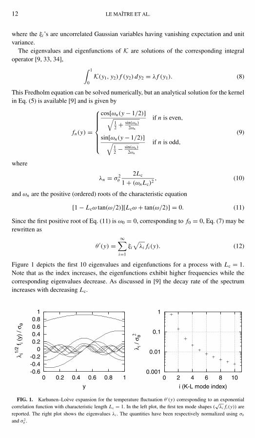
Figure 1 depicts the first 10 eigenvalues and eigenfunctions for a process with Lc = 1.Note that as the index increases, the eigenfunctions exhibit higher frequencies while thecorresponding eigenvalues decrease. As discussed in [9] the decay rate of the spectrumincreases with decreasing Lc.

-0.6-0.4-0.2

00.20.40.60.8

1

0 0.2 0.4 0.6 0.8 1

λ i1/

2 f i (

y) /

σ θ

y

0.001

0.01

0.1

1

0 2 4 6 8 10

λ i /

σ θ 2

i (K-L mode index)

FIG. 1. Karhunen–Loeve expansion for the temperature fluctuation θ ′(y) corresponding to an exponentialcorrelation function with characteristic length Lc = 1. In the left plot, the first ten mode shapes (

√λi fi (y)) are

reported. The right plot shows the eigenvalues λi . The quantities have been respectively normalized using σθ

and σ 2θ .


TABLE I

E2σ and E∞

σ for Various Values of NKL for Lc = 1/2, 1, and 2

NKL

4 6 10 20 40

E2σ (NKL) − Lc = 1/2 0.5882E−1 0.3751E−1 0.2161E−1 0.1045E−1 0.5129E−2

E2σ (NKL) − Lc = 1 0.2947E−1 0.1871E−1 0.1077E−1 0.5213E−2 0.2562E−2

E2σ (NKL) − Lc = 2 0.1473E−1 0.9337E−2 0.5376E−2 0.2604E−2 0.1280E−2

E∞σ (NKL) − Lc = 1/2 0.1076E−0 0.6592E−1 0.3453E−1 0.1300E−1 0.5590E−2

E∞σ (NKL) − Lc = 1 0.5346E−1 0.3255E−1 0.1704E−1 0.6429E−2 0.2792E−2

E∞σ (NKL) − Lc = 2 0.2657E−1 0.1615E−1 0.8456E−2 0.3197E−2 0.1395E−2

In numerical implementations, the KL expansion [Eq. (12)] is truncated, and the temper-ature “fluctuation” is approximated as

θ ′ =NKL∑i=1

ξi

√λi fi (y), (13)

where NKL is the number of modes retained in the computations. The error introduced bythis truncation is quantified in terms of the L p norms:

E pK(NKL) =

[ ∫ 1

0

∫ 1

0

∣∣∣∣∣K(y1, y2) −NKL∑i=1

λi fi (y1) f1(y2)

∣∣∣∣∣p

dy1 dy2

]1/p

, (14)

E pσ (NKL) =

∫ 1

0

∣∣∣∣∣σθ −√√√√ NKL∑

i=1

λi f 2i (y)

∣∣∣∣∣p

dy

1/p

. (15)

Table I reports E2σ and E∞

σ for different values of NKL and for Lc = 1/2, 1, and 2; Table IIprovides the corresponding values of E2

K and E∞K . The results indicate that at fixed NKL

the “truncation” errors scale approximately as 1/Lc. At fixed correlation length, E2σ and

E∞K decrease as N 1

KL, while E∞σ and E2

K exhibit faster decay rates. The effect of truncationof K is further illustrated in Fig. 2, which depicts the truncated correlation function andits deviation from the exact solution for Lc = 1. The results indicate that the truncationerror is mainly concentrated in a thin band around the axis y1 = y2 and that it exhibits rapid

TABLE II

E2K and E∞

K for Various Values of NKL for Lc = 1/2, 1, and 2

NKL

4 6 10 20 40

E2K(NKL) − Lc = 1/2 0.3366E−1 0.1791E−1 0.8176E−2 0.2988E−2 0.1249E−2

E2K(NKL) − Lc = 1 0.1736E−1 0.9076E−2 0.4107E−2 0.1496E−2 0.6247E−3

E2K(NKL) − Lc = 2 0.8789E−2 0.4562E−2 0.2057E−2 0.7882E−3 0.3124E−3

E∞K (NKL) − Lc = 1/2 0.2188E−0 0.1439E−0 0.8462E−1 0.4149E−1 0.2051E−1

E∞K (NKL) − Lc = 1 0.1127E−0 0.7285E−1 0.4250E−1 0.2076E−1 0.1026E−1

E∞K (NKL) − Lc = 2 0.5699E−1 0.3660E−1 0.2128E−1 0.1039E−1 0.5130E−2

14 LE MAITRE ET AL.

00.2

0.40.6

0.81

y1

00.2

0.40.6

0.81

y2

-0.03-0.02-0.01

00.010.020.030.040.050.060.070.08

Error on K(y1,y2)

00.2

0.40.6

0.81

y1

00.2

0.40.6

0.81

y2

0

0.2

0.4

0.6

0.8

1

K(y1,y2)

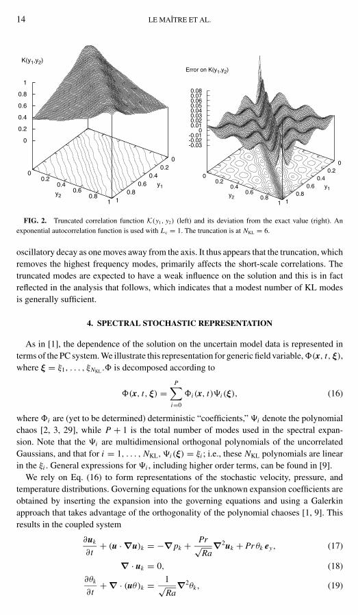
FIG. 2. Truncated correlation function K(y1, y2) (left) and its deviation from the exact value (right). Anexponential autocorrelation function is used with Lc = 1. The truncation is at NKL = 6.

oscillatory decay as one moves away from the axis. It thus appears that the truncation, whichremoves the highest frequency modes, primarily affects the short-scale correlations. Thetruncated modes are expected to have a weak influence on the solution and this is in factreflected in the analysis that follows, which indicates that a modest number of KL modesis generally sufficient.

4. SPECTRAL STOCHASTIC REPRESENTATION

As in [1], the dependence of the solution on the uncertain model data is represented interms of the PC system. We illustrate this representation for generic field variable, �(x, t, ξ),where ξ = ξ1, . . . , ξNKL .� is decomposed according to

�(x, t, ξ) =P∑

i=0

�i (x, t)�i (ξ), (16)

where �i are (yet to be determined) deterministic “coefficients,” �i denote the polynomialchaos [2, 3, 29], while P + 1 is the total number of modes used in the spectral expan-sion. Note that the �i are multidimensional orthogonal polynomials of the uncorrelatedGaussians, and that for i = 1, . . . , NKL, �i (ξ) = ξi ; i.e., these NKL polynomials are linearin the ξi . General expressions for �i , including higher order terms, can be found in [9].

We rely on Eq. (16) to form representations of the stochastic velocity, pressure, andtemperature distributions. Governing equations for the unknown expansion coefficients areobtained by inserting the expansion into the governing equations and using a Galerkinapproach that takes advantage of the orthogonality of the polynomial chaoses [1, 9]. Thisresults in the coupled system

∂uk

∂t+ (u · ∇u)k = −∇pk + Pr√

Ra∇2uk + Pr θk ey, (17)

∇ · uk = 0, (18)

∂θk

∂t+ ∇ · (uθ)k = 1√

Ra∇2θk, (19)


for k = 0, . . . , P . Here, uk(x, t), pk(x, t), and θk(x, t) are the coefficients in the PC expan-sion of the normalized velocity, pressure, and temperature fields, respectively. The quadraticvelocity–velocity and velocity–temperature products are given by

(u · ∇u)k =P∑

i=0

P∑j=0

Ci jkui∇u j (20)

and

(uθ)k =P∑

i=0

P∑j=0

Ci jkuiθ j , (21)

where

Ci jk ≡ 〈�i� j�k〉⟨�2

k

⟩ . (22)

Note that although Ci jk = 0 for 1 ≤ i, j, k ≤ NKL, it is generally nonvanishing, so that theGalerkin procedure results in a coupled system for the velocity and temperature modes.Note, however, that the velocity divergence constraints are decoupled, which enables us toadapt the SPM developed in [1]. This approach is outlined in the following sections.

4.1. Boundary Conditions

Following [1], boundary conditions are treated in a “weak sense”; i.e., the Galerkinapproach is also applied at the boundaries. In particular, the PC decomposition is alsointroduced into the corresponding expressions, and orthogonal projections are used to deriveboundary conditions for the velocity and temperature modes. For the setup outlined inSection 3, we obtain

uk = 0, k = 0, . . . , P ∀x ∈ ∂�, (23)

∂θk

∂y= 0, k = 0, . . . , P for y = 0 and y = 1, (24)

θ0(x = 0, y) = 1

2, θ0(x = 1, y) = −1

2, (25)

θk(x = 0, y) = 0, θk(x = 1, y) = √λk fk(y) for k = 1, . . . , NKL, (26)

θk(x = 0, y) = θk(x = 1, y) = 0 for k > NKL. (27)

Here � = [0, 1] × [0, 1] denotes the computational domain, and ∂� is its boundary.

4.2. Solution Method

As mentioned earlier, the solution scheme is an adapted version of the SPM introducedin [1]. Numerical integration of the governing equations of the stochastic mode follows anexplicit fractional step procedure that is based on first advancing the velocity and temperaturemodes using

uk = 4unk − un−1

k

3+ 2�t

3

[−2(u · ∇u)n

k + (u · ∇u)n−1k + Pr√

Ra∇2un

k + Pr θnk ey

], (28)

θn+1k = 4θn

k − θn−1k

3+ 2�t

3

[∇ · (−2(uθ)n

k + (uθ)n−1k

) + 1√Ra

∇2θnk

], (29)

16 LE MAITRE ET AL.

where superscripts refer to the time level and �t is the time step. Note that since we areprimarily interested in the steady-state solution of this system, we have combined explicitsecond-order time discretization of the convective terms and with first-order discretizationof the buoyancy and viscous terms. As in [1], spatial derivatives are approximated usingsecond-order centered differences. In the second fractional step, the “intermediate” velocitymodes uk are updated so as to satisfy the divergence constraints [35, 36]; we use

un+1k = uk − 2�t

3∇pn+1

k , (30)

where pk are solutions to the Poisson equations

∇2pn+1k = 3

2�t∇ · uk (31)

with homogeneous Neumann conditions [35, 36]. Note that these elliptic systems for thevarious modes are decoupled, a key feature in the efficiency of SPM [1].

In the implementations presented in the following, we relied on a conservative second-order finite-difference discretization on a uniform Cartesian mesh with (Nx , Ny) cells inthe x and y directions respectively. A direct, Fourier-based, fast Poisson solver is used toinvert Eqs. (31). Since these inversions account for the bulk of the CPU times, and sincesystems for individual modes are decoupled, the computational cost scales essentially asO(N log N ), where N ≡ Nx × Ny × (P + 1). This estimate is in fact reflected in the teststhat follow.

5. DETERMINISTIC PREDICTION

We start with a brief discussion of deterministic predictions, obtained by setting the order(NO) of the PC expansion to zero. In this case, the stochastic boundary conditions reduce tothose of the classical problem with uniform hot and cold wall temperatures, θh = 1/2 andθc = −1/2. The resulting predictions are used to validate the computations and to select a

FIG. 3. Scaled temperature field (left) and velocity vectors (right) for the deterministic temperature boundaryconditions (θh = −θc = 1/2) computed using zero-order spectral expansion (NO = 0).


suitable grid size. To this end, the results are compared with the spectral computations ofLe Quere [12]. For Ra = 106, Le Quere found a steady Nusselt number Nu = 8.8252, withthe Nusselt number defined by

Nu ≡ −∫ 1

0

∂θ

∂xdy. (32)

Following a systematic grid refinement study, we find that a computational grid withNx = 140 and Ny = 100 is sufficient for accurate predictions. Starting from an initial stateof rest, the computations are carried out until steady conditions are reached. Specifically,the computations are stopped when the maximum change in any field quantity falls below atolerance ε = 10−10. (Double precision arithmetic is used.) For the current grid resolution,the steady Nusselt number is found to be Nu = 8.8810, which is within 0.63% of theprediction of Le Quere. The structure of the steady field, depicted in Fig. 3, reveals thermalboundary layers on the hot and cold walls and a clockwise circulation of the fluid; thesepredictions are also in good agreement with the results reported in [12].

6. CONVERGENCE ANALYSIS

An analysis of the convergence of the spectral representation scheme is performed in thissection. Following the previous discussion, we are presently dealing with a two-parameterdiscretization that involves the number NKL of Karhunen–Loeve modes, as well as the orderNO of the PC expansion. As discussed in [9], the total number P of orthogonal polynomialsincreases monotonically with NKL and NO [9].

6.1. Convergence of KL Expansion

In Section 3, we observed that the KL expansion converged rapidly and consequentlyspeculated that truncation of this expansion would have little effect on the predictions. Wenow examine this expected trend by computing the mean Nusselt number,

Nu = −∫ 1

0

∂θ0

∂xdy, (33)

and its standard deviation,

σ(Nu) =(

P∑i=1

{[−∫ 1

0

∂θi

∂xdy

]2

〈ii 〉})1/2

, (34)

for NKL ranging from 2 to 10. For brevity, we restrict our attention to a first-order PCexpansion, and results are obtained with fixed Lc = 1 and σθ = 0.25.

The average of the local heat flux variance along the wall is given by

σ 2(∂θ/∂x) =∫ 1

0

P∑i=1

[∂θi

∂x

]2

〈ii 〉 dy. (35)

and should be carefully distinguished from σ 2(Nu). At steady state, the net heat flux on thehot wall equals that on the cold wall; since this relationship holds for arbitrary realization,

18 LE MAITRE ET AL.

TABLE III

Effect of NKL on Nu and σ(Nu) for NO = 1,

Lc = 1, and σθ = 0.25

NKL Nu σ(Nu) P

2 8.96344 2.47009 24 8.97114 2.46979 46 8.97179 2.46980 68 8.97190 2.46980 8

10 8.97192 2.46980 10

σ 2(Nu) has the same value on the hot wall as on the cold wall. On the other hand, σ 2(∂θ/∂x)

is expected to assume a higher value on the cold wall, where random fluctuations areimposed, than on the hot wall, since these fluctuations are expected to be smoothed out bydiffusion.

Computed values of Nu and σ(Nu) are reported in Table III. As expected, the results showthat for the present conditions Nu and σ(Nu) converge rapidly with NKL. To further examinethe predictions, we plot in Fig. 4 the distribution of the normalized heat flux −∂θ/∂x alongthe hot and cold walls as a function of P . (Note that for NO = 1, P = NKL.) Clearly, on thehot wall, only modes 0 and 1 contribute significantly to the local heat flux; for the highermodes, ∂θi/∂x is close to zero for all y. This situation contrasts with the distribution of theheat fluxes on the cold wall, where significant heat flux fluctuations are observed for all thePC modes. However, as noted earlier, the net heat fluxes across the hot and cold walls areequal at steady state. Thus, when integrated along the boundary, the significant fluctuationsof the higher modes on the cold wall tend to cancel out. This explains the rapid convergenceof integral quantities in Table III.

The standard deviation of the local heat flux, shown in Fig. 5, closely reflects thesetrends. In particular, by comparing points symmetrically across the midplane, the re-sults clearly show that the values on the cold wall are generally larger than those on thehot wall. Also note that the curve for the cold wall exhibits a noticeable waviness that

0

0.1

0.2

0.3

0.4

0.5

0.6

0.7

0.8

0.9

1

-5 0 5 10 15 20

y

-∂ θi / ∂ x

Cold-wall

0

0.1

0.2

0.3

0.4

0.5

0.6

0.7

0.8

0.9

1

-5 0 5 10 15 20

y

-∂ θi / ∂ x

Hot-wall

FIG. 4. Local heat fluxes versus y on the hot (left) and cold (right) walls, for modes 0–10. A first-orderexpansion is used with NKL = 10, Lc = 1, and σθ = 0.25.


0

0.1

0.2

0.3

0.4

0.5

0.6

0.7

0.8

0.9

1

0 1 2 3 4 5 6 7 8

y

<[ ∂ θ / ∂ x - <∂ θ / ∂ x> ]2 >1/2

Hot-wallCold-wall

FIG. 5. Standard deviation of the local heat fluxes versus y on the hot and cold walls. A first-order expansionis used with NKL = 10, Lc = 1, and σθ = 0.25.

corresponds to the imposed conditions, whereas the curve for the hot-wall distribution issmooth.

6.2. Convergence of PC Expansion

In this section, we analyze the convergence of the PC expansion by contrasting resultsobtained with NO = 1, 2, and 3. Results are obtaining with Lc = 1 and σθ = 0.25, usingboth four and six KL modes.

Wall heat transfer. The computed values of Nu and σ(Nu) are reported in Table IV,together with the number P of polynomials used. The results exhibit a fast convergence asthe order of the PC expansion, NO, increases. The differences in Nu and σ(Nu) betweensecond- and third-order solutions are less than 0.01% and 0.05%, respectively. The closequantitative agreement between the results for NO = 2 and 3 indicates that, at least as far asintegral quantities are concerned, a second-order expansion is sufficiently accurate. This fastconvergence rate is also indicative of the smooth dependence of the solution with respectto the imposed random temperature fluctuations.

Plotted in Fig. 6 are the heat flux distributions along the cold (top row) and hot (bottomrow) walls for NO = 1, 2, and 3. Results are obtained with NKL = 4 and curves are plotted

TABLE IV

Mean Nusselt Number and Its Standard Deviation for First-, Second-, and Third-Order

PC Expansion with NKL = 4 and 6 for Lc = 1 and σθ = 0.25

Nu σ(Nu) P

NO NKL = 4 NKL = 6 NKL = 4 NKL = 6 NKL = 4 NKL = 6

1 8.97114 8.97179 2.46979 2.46980 5 72 8.97289 8.97352 2.46323 2.46327 15 273 8.97337 8.97340 2.46239 2.46245 34 83

20 LE MAITRE ET AL.

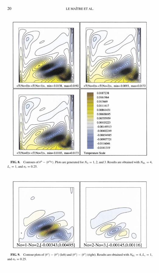
FIG. 8. Contours of θ 0 − 〈θ NO 〉. Plots are generated for NO = 1, 2, and 3. Results are obtained with NKL = 4,Lc = 1, and σθ = 0.25.

FIG. 9. Contour plots of 〈θ 1〉 − 〈θ 2〉 (left) and 〈θ 2〉 − 〈θ 3〉 (right). Results are obtained with NKL = 4, Lc = 1,and σθ = 0.25.


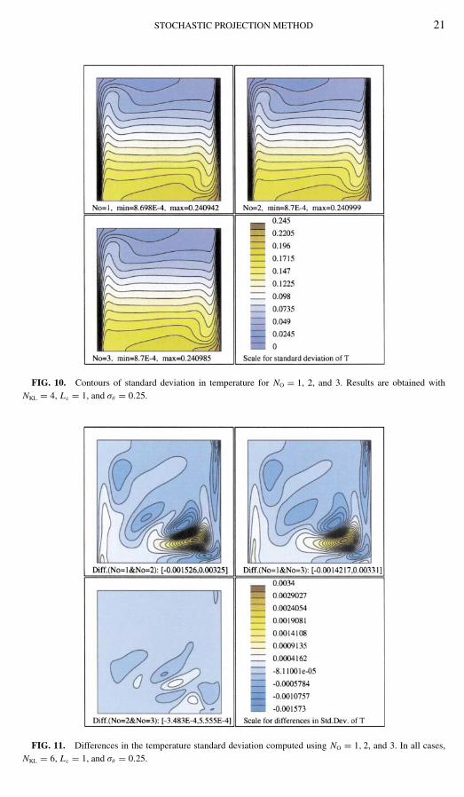
FIG. 10. Contours of standard deviation in temperature for NO = 1, 2, and 3. Results are obtained withNKL = 4, Lc = 1, and σθ = 0.25.

FIG. 11. Differences in the temperature standard deviation computed using NO = 1, 2, and 3. In all cases,NKL = 6, Lc = 1, and σθ = 0.25.

22 LE MAITRE ET AL.

FIG. 6. Local heat flux versus y on the cold (top row) and hot (bottom row) walls. Results are obtained withNKL = 4, Lc = 1, and σθ = 0.25. Curves are plotted for every mode in the PC expansion. P = 4 for NO = 1,P = 14 for NO = 2, and P = 34 for NO = 3.

for every mode in the PC expansion. The local heat flux profiles for the “first-order modes”(index i ≤ 4) have shapes similar to those reported in Fig. 4: these modes have significantamplitude on the cold wall, whereas modes higher than 2 are much less pronounced on thehot wall. On both walls, the first-order modes are slightly influenced by the order of the PCexpansion. Whereas increasing NO introduces more modes in the expansion (P = 14 forNO = 2 and P = 33 for NO = 3), the heat fluxes associated with these higher order modesare very low. Consequently, the “correction” of the local heat fluxes, arising when NO isincreased, is weak whenever NO > 1. This fact is also shown in Fig. 7, where the localheat-flux standard deviations are plotted for NO = 1, 2, and 3.

The present analysis of wall heat fluxes only shows how the solution converges, globallyor locally, on the vertical boundaries. To further investigate the behavior of the spectral

FIG. 7. Local standard deviation of the heat fluxes on the hot (left) and cold (right) walls, for NO = 1, 2,and 3. Results are obtained with NKL = 4, Lc = 1, and σθ = 0.25.


representation, we analyze the temperature and velocity fields within the cavity. We focusour attention on the distributions of mean quantities and their standard deviations andpostpone to Section 7 the examination of individual mode structure.

Temperature field. We start by noting that, since the natural convection in the cavityis not a linear process, the mean temperature distribution differs from the deterministicprediction corresponding to the mean temperature boundary condition, θc = −1/2. Thisdeterministic prediction, corresponding to ξi = 0, i = 1, . . . , NKL, shall be denoted by θ0.Meanwhile, we shall denote by 〈θ NO=1,2,3〉 ≡ θ0(NO) the mean predictions obtained usingfirst-, second-, and third-order PC expansions, respectively.

Examination of the mean temperature fields obtained with NO = 1, 2, and 3 (not shown)reveals that these fields have features like those of θ0 (shown earlier in Fig. 3). Thus,we have found it more convenient to analyze the difference fields θ0 − 〈θ NO≥1〉. Thesedifference fields are plotted in Fig. 8 for NKL = 4. A close agreement is observed betweenthe plots corresponding to the different expansion orders. Only a very weak dependence ofthe local magnitudes on NO can be detected. Thus, increasing NO has only a weak effecton the expected temperature field. To further demonstrate the convergence of the spectralrepresentation, the differences 〈θ NO=1〉 − 〈θ NO=2〉 and 〈θ NO=2〉 − 〈θ NO=3〉 are displayed inFig. 9. The results show that, at least as far as the mean field is concerned, the first-orderexpansion captures most of the effects of uncertainty. The difference 〈θ NO=2〉 − 〈θ NO=3〉 isvery small, indicating that the truncated terms have a weak impact on the mean temperature.

Figure 8 also shows that the mean temperature along the cold wall is higher than thatof θ0. The opposite situation is reported along the hot wall, where the mean temperatureis lowered by the uncertainty. These changes are responsible for the improvement of theglobal heat-transfer coefficient Nu. In addition, the mean temperature on the bottom of thecavity is significantly lower than that of θ0; in the upper part of the cavity, the mean anddeterministic predictions are nearly equal. To explain these trends, one notes that the meanclockwise flow circulation is not altered by the stochastic boundary conditions (as will beshown later). So, on average, the fluid is traveling downward along the cold wall, whereit is affected by random temperature conditions. The random fluctuations are transportedacross the cavity to the hot wall. As the fluid travels upward along the hot wall, uncertaintyis reduced due to diffusion, so that when reaching the upper part of the cavity, the fluidtemperature has lost most of its uncertainty, and its mean value is close to that of θ0. Wealso observe that the deviation of the mean temperature field from θ0 exhibits a complexstructure, with alternating signs, in the lower right quadrant, where the deviation from θ0

peaks. This pattern is closely correlated with the uncertainties in the velocity fields, as willbe further discussed.

Additional insight into the role of stochastic boundary conditions can be gained fromFig. 10, which depicts the temperature standard deviation fields for NO = 1, 2, and 3. Theresults show that the standard deviation distribution has a structure similar to that of themean, with two layers parallel to the vertical walls and a horizontal stratified arrangementfrom the bottom to the top of the cavity. The standard deviation vanishes on the hot wall,where deterministic conditions are imposed, and reaches its maximum on the cold wall, withvalues close to σθ . This spatial distribution is consistent with the arguments just presentedregarding the role of circulation in driving the uncertainty.

Finally, in Fig. 11, it is shown that the expansions for NO = 1, 2, and 3 provide essentiallythe same estimate of the temperature standard deviation, with differences in the fourth

24 LE MAITRE ET AL.

FIG. 17. Scaled temperature fields θk for k = 0, . . . , 14. Results are obtained with NKL = 4, NO = 2, Lc = 1,and σθ = 0.25.


FIG. 19. Scaled temperature fields θk for NKL = 4, obtained using NISP/GH predictions with Nd = 81. Lc = 1,and σθ = 0.25.

26 LE MAITRE ET AL.

FIG. 12. (a) Velocity map of the difference 〈uNO=3〉 − u0. (b) Profiles of mean horizontal velocity (〈uNO=3〉)and mean vertical velocity (〈vNO=3〉). The profiles are independently scaled for clarity. The scaled length ofthe bars corresponds to 6 times the local standard deviation. Results are obtained with NKL = 6, Lc = 1, andσθ = 0.25.

significant digit. These results also demonstrate the fast convergence rate of the spectralexpansion and the fact that in the present case a first-order expansion captures most of thestandard deviation.

Velocity field. As was done for the temperature distribution, we start by examiningthe deviation of the mean velocity field from u0, which denotes the deterministic solu-tion corresponding to the mean temperature condition (θc = −1/2). The mean velocityfields corresponding to first-, second-, and third-order PC expansions will be denoted by〈uNO=1,2,3〉, respectively. For each case, we find that the deviation of the mean solution fromu0 is small, and we consequently focus on the differences 〈uNO≥1〉 − u0.


FIG. 13. Velocity map of the difference 〈uNO=3〉 − 〈uNO=2〉. Results are obtained with NKL = 6, Lc = 1, andσθ = 0.25.

Figure 12a shows the distribution of 〈uNO=3〉 − u0 for a simulation with NKL = 6, Lc = 1,and σθ = 0.25. The difference field exhibits three complex structures that lie in the lowerpart of the cavity. While these structures resemble the recirculating eddies of the meanflow, it should be emphasized that the velocity magnitudes have been scaled by a factorof 10 compared to those in Fig. 3. Thus, with respect to u0, the mean field is significantlyperturbed in the regions occupied by these structures, but it is not actually recirculating.This can be verified by inspecting the mean solution itself, depicted in Fig. 12b, usingthe profiles of mean horizontal and mean vertical velocity. The profiles show that themean flow is not recirculating but that flow “reversal,” hence recirculation, in the lowerright corner is likely to occur. In this region, one observes large standard deviations andlow mean velocities, especially outside the boundary layers; this is indicative of largesensitivity to the stochastic boundary conditions. This trend is consistent with earlier ob-servations regarding the deviations θ0 − 〈θ NO≥1〉, which exhibited maxima at these samelocations.

To verify that the behavior of the stochastic solution is well represented, and consequentlythat the previously mentioned trends are not an artifact of the method, we inspect in Fig. 13the distribution of 〈uNO=3〉 − 〈uNO=2〉. The velocity map is generated with a scaling factorthat is 10 times larger than that used in Fig. 12a. The results clearly demonstrate that there arevery small differences between the second- and third-order solutions and that both provideaccurate representations of the stochastic process.

Remarks. We close this section with two remarks regarding the ability of the spectralrepresentation to accurately reproduce individual events and regarding the CPU costs of thespectral solution scheme.

Recall that the spectral representation relies on a weighted residual procedure to de-termine the mode coefficients. This representation is the closest polynomial to the exact

28 LE MAITRE ET AL.

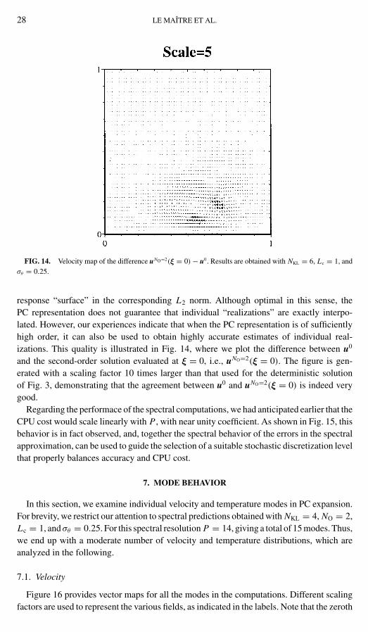
FIG. 14. Velocity map of the difference uNO=2(ξ = 0) − u0. Results are obtained with NKL = 6, Lc = 1, andσθ = 0.25.

response “surface” in the corresponding L2 norm. Although optimal in this sense, thePC representation does not guarantee that individual “realizations” are exactly interpo-lated. However, our experiences indicate that when the PC representation is of sufficientlyhigh order, it can also be used to obtain highly accurate estimates of individual real-izations. This quality is illustrated in Fig. 14, where we plot the difference between u0

and the second-order solution evaluated at ξ = 0, i.e., uNO=2(ξ = 0). The figure is gen-erated with a scaling factor 10 times larger than that used for the deterministic solutionof Fig. 3, demonstrating that the agreement between u0 and uNO=2(ξ = 0) is indeed verygood.

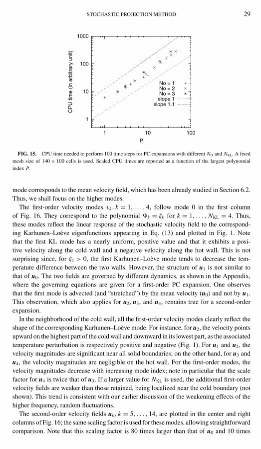
Regarding the performace of the spectral computations, we had anticipated earlier that theCPU cost would scale linearly with P , with near unity coefficient. As shown in Fig. 15, thisbehavior is in fact observed, and, together the spectral behavior of the errors in the spectralapproximation, can be used to guide the selection of a suitable stochastic discretization levelthat properly balances accuracy and CPU cost.

7. MODE BEHAVIOR

In this section, we examine individual velocity and temperature modes in PC expansion.For brevity, we restrict our attention to spectral predictions obtained with NKL = 4, NO = 2,Lc = 1, and σθ = 0.25. For this spectral resolution P = 14, giving a total of 15 modes. Thus,we end up with a moderate number of velocity and temperature distributions, which areanalyzed in the following.

7.1. Velocity

Figure 16 provides vector maps for all the modes in the computations. Different scalingfactors are used to represent the various fields, as indicated in the labels. Note that the zeroth


1

10

100

1000

1 10 100

CP

U ti

me

(in a

rbitr

ary

unit)

P

No = 1No = 2No = 3slope 1

slope 1.1

FIG. 15. CPU time needed to perform 100 time steps for PC expansions with different NO and NKL. A fixedmesh size of 140 × 100 cells is used. Scaled CPU times are reported as a function of the largest polynomialindex P.

mode corresponds to the mean velocity field, which has been already studied in Section 6.2.Thus, we shall focus on the higher modes.

The first-order velocity modes vk, k = 1, . . . , 4, follow mode 0 in the first columnof Fig. 16. They correspond to the polynomial k = ξk for k = 1, . . . , NKL = 4. Thus,these modes reflect the linear response of the stochastic velocity field to the correspond-ing Karhunen–Loeve eigenfunctions appearing in Eq. (13) and plotted in Fig. 1. Notethat the first KL mode has a nearly uniform, positive value and that it exhibits a posi-tive velocity along the cold wall and a negative velocity along the hot wall. This is notsurprising since, for ξ1 > 0, the first Karhunen–Loeve mode tends to decrease the tem-perature difference between the two walls. However, the structure of u1 is not similar tothat of u0. The two fields are governed by different dynamics, as shown in the Appendix,where the governing equations are given for a first-order PC expansion. One observesthat the first mode is advected (and “stretched”) by the mean velocity (u0) and not by u1.This observation, which also applies for u2, u3, and u4, remains true for a second-orderexpansion.

In the neighborhood of the cold wall, all the first-order velocity modes clearly reflect theshape of the corresponding Karhunen–Loeve mode. For instance, for u2, the velocity pointsupward on the highest part of the cold wall and downward in its lowest part, as the associatedtemperature perturbation is respectively positive and negative (Fig. 1). For u1 and u2, thevelocity magnitudes are significant near all solid boundaries; on the other hand, for u3 andu4, the velocity magnitudes are negligible on the hot wall. For the first-order modes, thevelocity magnitudes decrease with increasing mode index; note in particular that the scalefactor for u4 is twice that of u3. If a larger value for NKL is used, the additional first-ordervelocity fields are weaker than those retained, being localized near the cold boundary (notshown). This trend is consistent with our earlier discussion of the weakening effects of thehigher frequency, random fluctuations.

The second-order velocity fields uk, k = 5, . . . , 14, are plotted in the center and rightcolumns of Fig. 16; the same scaling factor is used for these modes, allowing straightforwardcomparison. Note that this scaling factor is 80 times larger than that of u0 and 10 times

30 LE MAITRE ET AL.

FIG. 16. Velocity fields uk for k = 0, . . . , 14. Results are obtained with NKL = 4, NO = 2, Lc = 1, andσθ = 0.25. Note that different velocity scales are used, as indicated in the labels.


larger than that of u4. Thus, the magnitudes of the second-order velocity fields are muchsmaller than those of zeroth- and first-order modes. This rapid decay also reflects the rapidconvergence of the PC expansion.

The second-order velocity modes have very different patterns, some being only significantalong the cold wall and others affecting the entire cavity. Some of these structures can beeasily interpreted. For example. u5, which corresponds to 5 = ξ 2

1 − 1, has a structuresimilar to that of u1. For other modes, the structure of the corresponding velocity fields arequite complex and difficult to interpret. It is interesting to note, however, that the velocityfields involving the second KL mode (u6, u9, u10, and u11) seem to have the most significantmagnitudes, suggesting that this mode has greater impact on the stochastic process than theothers. On the other hand, second-order polynomials associated with the fourth KL modeappear to be very weak.

7.2. Temperature

Figure 17 shows contour plots of the temperature modes θk, k = 0, . . . , 14. Since themean temperature field θ0 has been analyzed earlier, we will focus on first- and second-order modes.

The contours of the first mode, θ1, are similar to those of θ0, even though the correspondingvalues differ. This is not surprising since these two modes obey similar boundary conditions,with θ0 being subjected to a uniform Dirichlet condition on the cold wall, while θ1 is nearlyuniform there. However, some differences between the distributions of θ1 and θ0 can beobserved at the lower right corner of the cavity. These differences appear to be governedby the circulation of the mean flow in the cavity. To appreciate this effect, we note that itis the mean field u0 which contributes to the transport of θ1; the heat flux associated withu1, which points upward near the cold wall, is dependent on the mean temperature field θ0

(see the Appendix). The role of the mean field in the transport of θ2, θ3, and θ4 can also beappreciated from the corresponding contour plots. Note that θ2, θ3, and θ4 are very smallin the upper half of the cavity but have significant values in the lower part of the cavityand/or in the vicinity of the cold wall. In particular, for θ3 and θ4 one observes fluctuationsof alternating sign that are localized near the cold boundary and that coincide with the shapeof the corresponding KL mode.

As for velocity, the second-order temperature modes are more difficult to interpret thanthe first-order modes. The only structures that can be easily identified are the imposed cold-wall distributions. The results indicate that significant mode coupling occurs, which can bedetected by inspecting the modes involving mixed products of the ξi ’s. For instance, for θ7 asecond-order coupling between ξ1 and ξ3 is involved; this mode exhibits three distinct zonesalong the cold wall, which reflect the shape of the third mode in the KL expansion. Apartfrom such identifiable features, the second-order modes can have complex distributions,some of which are localized in the lower part of the cavity, while others extend throughoutthe domain.

Regarding the amplitude of the second-order modes, we note those modes involv-ing ξ2 and ξ3, i.e., the second and third KL eigenfunctions, are dominant. Thus, not allsecond-order modes contribute equally to the stochastic process. In general, however, thesecond-order temperature modes are at least one order of magnitude lower than the first-order modes. This is consistent with earlier observations regarding the convergence of theexpansion.

32 LE MAITRE ET AL.

8. NONINTRUSIVE SPECTRAL PROJECTION

To verify the spectral computations of the previous section, a NISP approach is developed.The starting point in NISP is the observation that the modes ui and Ti can be obtained byprojecting deterministic computations onto the PC basis. If ud(ξ) and T d(ξ) denote thedeterministic solution corresponding to a particular realization ξ = (ξ1, . . . , ξNKL ), then thepolynomial coefficients are, by definition, given by

(ui , Ti ) = 〈(u, T )di 〉〈ii 〉 ≡

∫ ∞

−∞dξ1 · · ·

∫ ∞

−∞dξNKL

[(u, T )d(ξ)

i (ξ)⟨2

i

⟩ NKL∏k=1

exp(−ξ 2

k /2)

√2π

].

(36)

8.1. Gauss–Hermite Quadrature

For moderate values of NKL, our multidimensional integration can be efficiently per-formed using Gauss–Hermite quadrature [30, 31]. Using n collocation points along each“stochastic direction,” Eq. (36) can be approximated as

(ui , Ti ) =n∑

n1=1

. . .

n∑nNKL =1

(u, T )d(xn1 , . . . , xnNKL

)i(xn1 , . . . , xnNKL

)〈ii 〉

NKL∏k=1

wnk , (37)

where (xk, wk), k = 1, . . . , n, denote the one-dimensional GH integration points andweights. The quadrature in (37) is exact when the integrand is a polynomial of degreeof 2n − 1 or less. Thus, the coefficients can be exactly estimated if the process is spannedby polynomials of degree less than or equal to (2n − 1)/2. In this situation, the numberof deterministic realizations Nd required in the NISP approach for given NKL and NO isNd = (2NO − 1)NKL . It should be emphasized that for arbitrary NKL and NO, Nd is alwaysgreater than P, the number of polynomials in the spectral approach used here. Since theCPU time in the spectral approach is approximately P times that of a deterministic solu-tion, NISP is not as efficient as the spectral approach. Its main advantage, however, is thatit makes use of a deterministic solver without the need for any modifications and so is“nonintrusive.”

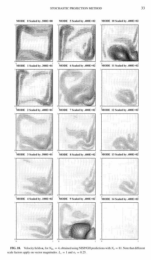
NISP/GH computations are performed for a case with NKL = 4 and NO = 2. We usen = 3 and so obtain Nd = 81 deterministic realizations for the corresponding GH quadraturepoints. (In contrast, the intrusive spectral approach discussed previously has P = 14, fora total of 15 modes.) Velocity and temperature modes obtained using NISP are plottedin Figs. 18 and 19, respectively. The corresponding results obtained using the intrusivespectral approach were given in Figs. 16 and 17 and have extensively discussed in theprevious section.

For the velocity fields, we find an excellent agreement between the intrusive spectralresults (Fig. 16) and the NISP predictions (Fig. 18) for the zeroth- and first-order modes.For the second-order modes (uk, k = 5, . . . , 14), small deviations are observed between thetwo sets, but the primary structure of the modes is quite similar. These small deviations arepronounced for coupled modes involving ξ2 and ξ3; the deviations are substantially smallerfor the nonmixed quadratic modes. Despite these small deviations, the agreement betweenthe intrusive and NISP/GH predictions is very satisfactory.


0 10

1

MODE 0 Scaled by .500E+00

0 10

1


0 10

1


0 10

1


0 10

1


0 10

1


0 10

1


0 10

1


0 10

1


0 10

1


0 10

1


0 10

1


0 10

1


0 10

1


0 10

1


FIG. 18. Velocity fields uk for NKL = 4, obtained using NISP/GH predictions with Nd = 81. Note that differentscale factors apply on vector magnitudes. Lc = 1 and σθ = 0.25.

34 LE MAITRE ET AL.

Comparison of the temperature modes in Figs. 19 and 17 reveal trends similar to thoseof the velocity modes. In particular, the zeroth- and first-order modes are in excellentquantitative agreement, as can be appreciated by inspecting the maxima and minima reportedon individual frames. These values also provide a good illustration of the deviations observedin the second-order modes. Again the largest differences are observed for modes involvingmixed products. The small magnitude of these differences, compared to the characteristicvalues of the first-order terms, is evident and should be emphasized.

The origin of deviations between intrusive and NISP/GH predictions can be traced tothe errors inherent in both approaches. These primarily consist of spectral truncation errorsin the intrusive approach and aliasing errors in the NISP predictions. Obviously, completeagreement between NISP and spectral computations can only be achieved in the case of afinite spectrum. Since we are presently dealing with second-order spectral representations,agreement would occur if the third- and higher order modes vanish identically, which isclearly not the case: the third-order terms are very small, but not identically vanishing.

To further examine these differences, we rely on the L2 norms of the differences betweenthe same temperature modes in two different solutions, T (1) and T (2), defined according to

E2ik ≡

[ ∫ ∫ (T (1)

i − T (2)k

)2dx dy

]1/2

. (38)

The indices i and k are selected so that i in the PC expansion of T (1) referes to the samepolynomical k in the polynomial expansion for T (2). Obviously, i = k when T (1) and T (2)

have the same number of KL modes, NKL.We have first compared modal solutions obtained with intrusive spectral computations

using the same order PC expansion but different number of KL modes. In this case, the errormeasure is only relevant for the modes that are shared in both representations, namely, thosebelonging to the expansion having lower NKL value. A sample of this exercise is shownin Fig. 20, which shows the L2 norm between temperature modes obtained using second-order expansions with NKL = 4 and 6. As is evident in the figure, the L2 errors between the

1e-07

1e-06

1e-05

0.0001

0 2 4 6 8 10 12 14

L2 n

orm

of d

iffer

ence

Polynomial index for NKL=4

FIG. 20. L2 norm of the difference in the common temperature modes obtained with intrusive spectralcalculations using NKL = 4 and NKL = 6. In both cases, a second-order PC expansion is used.


1e-05

0.0001

0.001

0 2 4 6 8 10 12 14

L2 n

orm

of d

iffer

ence

s

Polynomial Index for NKL =4

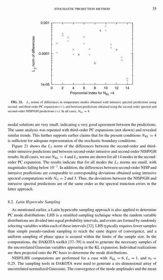
FIG. 21. L2 norms of differences in temperature modes obtained with intrusive spectral predictions usingsecond- and third-order PC expansions (+), and between predictions obtained using the second-order spectral andsecond-order NISP/GH predictions (×). In all cases, NKL = 4.

modal solutions are very small, indicating a very good agreement between the predictions.The same analysis was repeated with third-order PC expansions (not shown) and revealedsimilar trends. This further supports earlier claims that for the present conditions NKL = 4is sufficient for adequate representation of the stochastic boundary conditions.

Figure 21 shows the L2 norm of the differences between the second-order and third-order intrusive predictions and between second-order intrusive and second-order NISP/GHresults. In all cases, we use NKL = 4 and L2 norms are shown for all 14 modes in the second-order PC expansion. The results indicate that for all modes the L2 norms are small, withmagnitudes falling below 10−3. In addition, the differences between second-order NISP andintrusive predictions are comparable to corresponding deviations obtained using intrusivespectral computations with NO = 2 and 3. Thus, the deviations between the NISP/GH andintrusive spectral predictions are of the same order as the spectral trunction errors in thelatter approach.

8.2. Latin Hypercube Sampling

As mentioned earlier, a Latin hypercube sampling approach is also applied to determinePC mode distributions. LHS is a stratified sampling technique where the random variabledistributions are divided into equal probability intervals, and events are formed by randomlyselecting variables within each of these intervals [32]. LHS typically requires fewer samplesthan simple pseudo-random sampling to reach the same degree of convergence, and auniform sampling of phase space is assured within the limits of the sample size. In thecomputations, the DAKOTA toolkit [37–39] is used to generate the necessary samples ofthe uncorrelated Gaussian variables appearing in the KL expansion. Individual realizationsare then projected onto the PC basis to determine the mode distributions.

NISP/LHS computations are performed for a case with NKL = 6, Lc = 1, and σθ =0.25. The sampling tools in DAKOTA were used to generate a six-dimensional array ofuncorrelated normalized Gaussians. The convergence of the mode amplitudes and the mean

36 LE MAITRE ET AL.

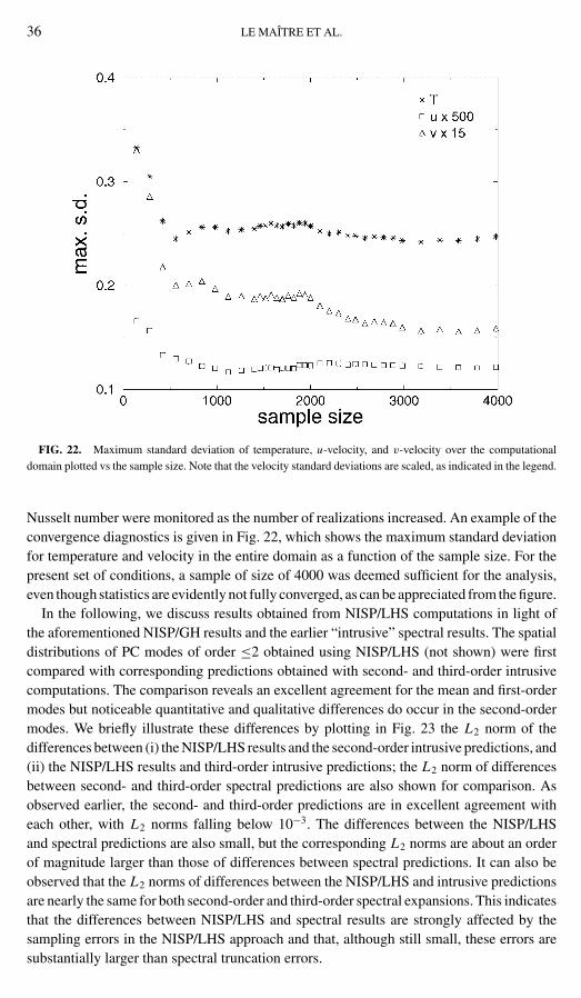
FIG. 22. Maximum standard deviation of temperature, u-velocity, and v-velocity over the computationaldomain plotted vs the sample size. Note that the velocity standard deviations are scaled, as indicated in the legend.

Nusselt number were monitored as the number of realizations increased. An example of theconvergence diagnostics is given in Fig. 22, which shows the maximum standard deviationfor temperature and velocity in the entire domain as a function of the sample size. For thepresent set of conditions, a sample of size of 4000 was deemed sufficient for the analysis,even though statistics are evidently not fully converged, as can be appreciated from the figure.

In the following, we discuss results obtained from NISP/LHS computations in light ofthe aforementioned NISP/GH results and the earlier “intrusive” spectral results. The spatialdistributions of PC modes of order ≤2 obtained using NISP/LHS (not shown) were firstcompared with corresponding predictions obtained with second- and third-order intrusivecomputations. The comparison reveals an excellent agreement for the mean and first-ordermodes but noticeable quantitative and qualitative differences do occur in the second-ordermodes. We briefly illustrate these differences by plotting in Fig. 23 the L2 norm of thedifferences between (i) the NISP/LHS results and the second-order intrusive predictions, and(ii) the NISP/LHS results and third-order intrusive predictions; the L2 norm of differencesbetween second- and third-order spectral predictions are also shown for comparison. Asobserved earlier, the second- and third-order predictions are in excellent agreement witheach other, with L2 norms falling below 10−3. The differences between the NISP/LHSand spectral predictions are also small, but the corresponding L2 norms are about an orderof magnitude larger than those of differences between spectral predictions. It can also beobserved that the L2 norms of differences between the NISP/LHS and intrusive predictionsare nearly the same for both second-order and third-order spectral expansions. This indicatesthat the differences between NISP/LHS and spectral results are strongly affected by thesampling errors in the NISP/LHS approach and that, although still small, these errors aresubstantially larger than spectral truncation errors.


FIG. 23. L2 norm of differences in temperature modes obtained with intrusive spectral predictions usingsecond- and third-order PC expansions (+), intrusive second-order and NISP/LHS with 4000 realizations (×),and intrusive third-order and NISP/LHS with 4000 realizations (�). In all cases, NKL = 6, and the comparison isrestricted to second-order modes.

Additional insight into the convergence of the NISP/LHS computations can be gainedfrom Fig. 24, which shows the L2 norm of the differences in mode distributions betweenthe NISP/LHS and second-order intrusive results, as a function of the sample size. Plottedin Fig. 24a are L2 norms for the mean and first-order modes; results for modes 7–13 areshown in Fig. 24b. Generally, the difference between NISP/LHS and spectral predictionsdiminishes quickly, but a residual difference remains for all modes as the sample sizeincreases. The difference decays quicker for the mean and the first-order modes (Fig. 24a),than for modes 7–13 (Fig. 24b). As can be observed in Fig. 23, the differences betweenNISP/LHS and intrusive spectral predictions are such that L2 norms corresponding to themean and first-order modes are comparable to or smaller than those corresponding to someof the second-order modes. Since the latter are significantly weaker than the former, thisindicates that the NISP/LHS predictions of the higher order modes have large relative errorsand are not well converged. This also shows that the sampling errors in NISP/LHS are behindthe observed differences in the distributions of second-order modes.

9. UNCERTAINTY QUANTIFICATION

We conclude this study with a quantitative analysis of the effects of the stochastic bound-ary conditions on heat transfer statistics within the cavity. We rely on spectral computationsusing NKL = 6, NO = 2, and a 140 × 100 computational grid. Results are obtained forthree different correlation lengths and standard deviations, namely, Lc = 0.5, 1, and 2 andσθ = 0.125, 0.25, and 0.5.

Computed values of Nu and σ(Nu) are reported in Tables V and VI, respectively. Table Vprovides the mean Nusselt number along with the difference Nu − Nu0, where Nu0 denotesthe Nusselt number corresponding to the deterministic prediction with θc = −1/2. Theresults show that Nu is larger than Nu0. For fixed correlation length, Nu − Nu0 increases

38 LE MAITRE ET AL.

FIG. 24. L2 norm of differences in temperature modes obtained with second-order intrusive and NISP/LHSpredictions for different sample size: (a) modes 0–6, (b) modes 7–13. In both approaches, NKL = 6, Lc = 1, andσθ = 0.25.

approximately as σ 2θ . In contrast, Nu exhibits as weaker dependence on Lc. This is not

surprising since, in the range considered, the eigenvalues λi of KL modes vary slowly withthe correlation length.

Unlike Nu, for fixed Lc the standard deviation σ(Nu) exhibits an approximately lineardependence on σθ , as shown in Table VI. Furthermore, compared with the mean, σ(Nu)

exhibits a more pronounced dependence on Lc. This trend is consistent with variations of


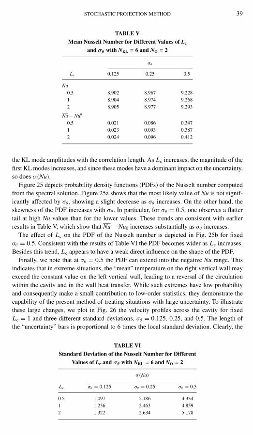
TABLE V

Mean Nusselt Number for Different Values of Lc

and σθ with NKL = 6 and NO = 2

σθ

Lc 0.125 0.25 0.5

Nu0.5 8.902 8.967 9.2281 8.904 8.974 9.2682 8.905 8.977 9.293

Nu − Nu0

0.5 0.021 0.086 0.3471 0.023 0.093 0.3872 0.024 0.096 0.412

the KL mode amplitudes with the correlation length. As Lc increases, the magnitude of thefirst KL modes increases, and since these modes have a dominant impact on the uncertainty,so does σ(Nu).

Figure 25 depicts probability density functions (PDFs) of the Nusselt number computedfrom the spectral solution. Figure 25a shows that the most likely value of Nu is not signif-icantly affected by σθ , showing a slight decrease as σθ increases. On the other hand, theskewness of the PDF increases with σθ . In particular, for σθ = 0.5, one observes a flattertail at high Nu values than for the lower values. These trends are consistent with earlierresults in Table V, which show that Nu − Nu0 increases substantially as σθ increases.

The effect of Lc on the PDF of the Nusselt number is depicted in Fig. 25b for fixedσθ = 0.5. Consistent with the results of Table VI the PDF becomes wider as Lc increases.Besides this trend, Lc appears to have a weak direct influence on the shape of the PDF.

Finally, we note that at σθ = 0.5 the PDF can extend into the negative Nu range. Thisindicates that in extreme situations, the “mean” temperature on the right vertical wall mayexceed the constant value on the left vertical wall, leading to a reversal of the circulationwithin the cavity and in the wall heat transfer. While such extremes have low probabilityand consequently make a small contribution to low-order statistics, they demonstrate thecapability of the present method of treating situations with large uncertainty. To illustratethese large changes, we plot in Fig. 26 the velocity profiles across the cavity for fixedLc = 1 and three different standard deviations, σθ = 0.125, 0.25, and 0.5. The length ofthe “uncertainty” bars is proportional to 6 times the local standard deviation. Clearly, the

TABLE VI

Standard Deviation of the Nusselt Number for Different

Values of Lc and σθ with NKL = 6 and NO = 2

σ(Nu)

Lc σθ = 0.125 σθ = 0.25 σθ = 0.5

0.5 1.097 2.186 4.3341 1.236 2.463 4.8592 1.322 2.634 5.178

40 LE MAITRE ET AL.

FIG. 25. PDFs of the Nusselt number computed from the spectral simulations using NKL = 6 and NO = 2:(a) Lc = 1 and σθ = 0.125, 0.25, and 0.5; (b) σθ = 0.5 and Lc = 0.5, 1, and 2.

FIG. 26. Mean velocity profiles across the cavity for σθ = 0.125 (left), 0.25 (center), and 0.5 (right). Theerror bars correspond to 6 times the local standard deviation. The same scaling is used for all three plots. Spectralresults with Lc = 1, NKL = 6, and NO = 2 are used.


uncertainty bars increase as σθ increases. In particular, for σθ = 0.5 the uncertainty barssuggest that events with upward velocity near the cold wall become probable. In contrast,one observes that the mean flow field is not strongly affected by σθ .

10. CONCLUSIONS

In this paper, the SPM [1] has been generalized to account for stochastic input datagenerated by a stochastic process. The Karhunen–Loeve expansion is used to representthe stochastic input data. The dependence of the solution process on the random data isexpressed in terms of the polynomial chaos system and the coefficients of the solution aredetermined using a weighted residual approach. The resulting stochastic formulation is in-corporated into a finite-difference projection method, which results in an efficient stochasticsolver.

The properties of the stochastic solver are analyzed in light of computed results for naturalconvection within a closed square cavity under stochastic temperature boundary conditions.In particular, the setup is used to examine the convergence properties of the spectral un-certainty representation scheme in terms of the number of KL modes and the order of thePC expansion. Computations are performed for a steady flow regime with Rayleigh num-ber of 106. For the selected conditions, the results indicate that the spectral representationconverges rapidly, providing accurate results for a second-order expansion using as few asfour KL modes. Numerical tests indicate that the CPU cost of the stochastic computationsis essentially proportional to the number of modes used in the spectral representration, thushighlighting the efficiency of the stochastic model.

To verify the spectral predictions, stand-alone deterministic computations are performedand are used in conjunction with “nonintrusive” spectral projection approaches. Two variantsof the NISP approach are implemented, one based on high-order Gauss–Hermite integra-tion and the other on a Latin hypercube sampling strategy. Results obtained using Gaussquadrature are in excellent agreement with the spectral predictions, showing very smalldifferences that are of the order of the spectral truncation errors. Predictions obtained usingthe Latin hypercube sampling scheme are also in agreement with the spectral predictionsbut exhibit differences that are an order of magnitude higher than those obtained usingGauss–Hermite quadrature. The verification study underscores the efficiency of the spec-tral computations, as the number of indepedent realizations needed to adequately representthe stochastic process is substatially higher than the corresponding number of PC modes.The analysis also shows that the nonintrusive approach based on Gauss–Hermite quadraturecan be significantly more attractive than that using Latin hypercube sampling, at least forproblems with a moderate number of stochastic dimensions.

The computations are used to quantify the effects of stochastic temperature conditionson the global heat transfer characteristics within the cavity. The results indicate that themean Nusselt number, Nu, is generally larger than Nu0, the Nusselt number correspondingto the mean (uniform) temperature profile. In particular, the difference Nu − Nu0 is foundto increase quadratically with σθ , the standard deviation of the stochastic temperature pro-file, but shows a weak dependence on the correlation length Lc. Meanwhile, the standarddeviation of the Nusselt number exhibits an approximately linear dependence on σθ and amore pronounced dependence on Lc than the mean Nusselt number.

So far, implementations of SPM have been restricted to flow conditions having relativelysimple physical models, involving quadratic nonlinearities only. In other situations, more

42 LE MAITRE ET AL.

complex physical models may arise that involve higher order nonlinearities. These resultin additional computational challenges for the present approach, particularly regarding theimplementation of the Galerkin scheme. Extensions that address these challenges in thecontext of chemically reacting flows are currently being developed.

APPENDIX

A first-order expansion gives a spectral basis involving a set of P + 1 = NKL + 1 or-thogonal polynomials:

0 = 1, i = ξi for i = 1, . . . , NKL = P. (39)

The governing equations for the zeroth-order velocity and temperature modes are

∂u0

∂t+

NKL∑i=0

ui · ∇ui = −∇p0 + Pr√Ra

∇2u0, (40)

∂θ0

∂t+

NKL∑i=0

∇ · (uiθi ) = 1√Ra

∇2θ0. (41)

For k = 1, . . . , NKL the governing equations can be expressed as

∂uk

∂t+ u0∇uk + uk∇u0 = −∇pk + Pr√

Ra∇2uk, (42)

∂θk

∂t+ ∇ · (u0θk + ukθ0) = 1√

Ra∇2θk . (43)

Meanwhile, continuity gives

∇ · uk = 0, k = 0, . . . , NKL. (44)

The velocity boundary conditions are given by

uk(x, t) = 0 ∀x ∈ ∂�, ∀t and k = 0, . . . . , NKL, (45)

while the scaled temperature boundary conditions are

θ0(x = 0, y) = 1/2, θ0(x = 1, y) = −1/2, (46)

θk(x = 0, y) = 0, θk(x = 1, y) =√

λk fk(y) for k = 1, . . . . , NKL, (47)

and

∂θk

∂y= 0 for y = 0, 1 and k = 0, . . . . , NKL. (48)

The first-order PC expansion thus leads to a set of NKL + 1 coupled momentum and heatequations and a set of NKL + 1 decoupled divergence constraints.


ACKNOWLEDGMENTS

This work was supported by the Laboratory Directed Research and Development Program at Sandia NationalLaboratories, funded by the U.S. Department of Energy. Support was also provided by the Defense AdvancedResearch Projects Agency (DARPA) and Air Force Research Laboratory, Air Force Materiel Command, USAF,under agreement F30602-00-2-0612. The U.S. government is authorized to reproduce and distribute reprints forGovernmental purposes notwithstanding any copyright annotation thereon. Computations were performed at theNational Center for Supercomputer Applications.

REFERENCES

1. O. P. Le Maıtre, O. M. Knio, H. N. Najm, and R. G. Ghanem, A stochastic projection method for fluid flow.I. Basic formulation, J. Comput. Phys. 173, 480 (2001).

2. S. Wiener, The homogeneous chaos, Am. J. Math. 60, 897 (1938).

3. R. H. Cameron and W. T. Martin, The orthogonal development of nonlinear functionals in series of Fourier–Hermite functionals, Ann. Math. 48, 385 (1947).

4. A. J. Chorin, Hermite expansions in Monte-Carle computation, J. Comput. Phys. 8, 472 (1971).

5. F. H. Maltz and D. L. Hitzl, Variance reduction in Monte Carlo computations using multi-dimensional Hermitepolynomials, J. Comput. Phys. 32, 345 (1979).

6. W. C. Meecham and D. T. Jeng, Use of the Wiener–Hermite expansion for nearly normal turbulence, J. FluidMech. 32, 225 (1968).

7. S. C. Crow and G. H. Canavan, Relationship between a Wiener–Hermite expansion and an energy cascade,J. Fluid Mech. 41, 387 (1970).

8. A. J. Chorin, Gaussian fields and random flow, J. Fluid Mech. 63, 21 (1974).

9. R. G. Ghanem and P. D. Spanos, Stochastic Finite Elements: A Spectral Approach (Springer-Verlag,Berlin/New York, 1991).

10. G. De Vahl Davis and I. P. Jones, Natural convection in a square cavity: A comparison exercice, Int. J. Numer.Methods Fluids 3, 227 (1983).

11. P. Le Quere and T. Alziary de Roquefort, Computation of natural-convection in two-dimensional cavities withTschebyscheff polynomials, J. Comput. Phys. 57, 210 (1985).

12. P. Le Quere, Accurate solution to the square thermally driven cavity at high Rayleigh number, Comput. Fluids20(1), 29 (1991).

13. D. R. Chenoweth and S. Paolucci, Natural convection in an enclosed vertical layer with large horizontaltemperature differences, J. Fluid Mech. 169, 173 (1986).

14. P. Le Quere, R. Masson, and P. Perrot, A Chebyshev collocation algorithm for 2D non-Boussinesq convection,J. Comput. Phys. 103, 320 (1992).

15. H. Paillere and P. Le Quere, Modelling and simulation of natural convection flows with large temperaturedifferences: A benchmark problem for low Mach number solvers, presented at 12th Seminar “ComputationalFluid Dynamics” CEA/Nuclear Reactor Division, Saclay, France 2000.

16. M. Christon, P. Gresho, and S. Sutton, Computational predictability of natural convection flows in enclosure,in Computational Fluid and Solid Mechanics, edited by K. Bathe, Proceedings of First MIT Conference onComputational Fluid and Solid Mechanics (Elsevier, Amsterdam, 2001), pp. 1465–1468.

17. D. M. Christopher, Numerical prediction of natural convection flows in a tall enclosure, in ComputationalFluid and Solid Mechanics, edited by K. Bathe, Proceedings of First MIT Conference on Computational Fluidand Solid Mechanics (Elsevier, Amsterdam, 2001), pp. 1469–1471.

18. G. Comini, M. Manzan, C. Nonino, and O. Saro, Finite element solutions for natural convection in a tallrectangular cavity, in Computational Fluid and Solid Mechanics, edited by K. Bathe, Proceedings of FirstMIT Conference on Computational Fluid and Solid Mechanics (Elsevier, Amsterdam, 2001), pp. 1472–1476.

19. G. Groce and M. Favero, Simulation of natural convection flow in enclosures by an unstaggered grid Finitevolume algorithm, in Computational Fluid and Solid Mechanics, edited by K. Bathe, Proceedings of FirstMIT Conference on Computational Fluid and Solid Mechanics (Elsevier, Amsterdam, 2001), pp. 1477–1481.

44 LE MAITRE ET AL.

20. P. M. Gresho and S. Sutton, 8:1 thermal cavity problem, in Computational Fluid and Solid Mechanics, editedby K. Bathe, Proceedings of First MIT Conference on Computational Fluid and Solid Mechanics (Elsevier,Amsterdam, 2001), pp. 1482–1485.

21. H. Johnston and R. Krasny, Computational predictability of natural convection flows in enclosures: A bench-mark problem, in Computational Fluid and Solid Mechanics, edited by K. Bathe, Proceedings of First MITConference on Computational Fluid and Solid Mechanics (Elsevier, Amsterdam, 2001), pp. 1486–1489.

22. S.-E. Kim and D. Choudhury, Numerical investigation of laminar natural convection flow inside a tall cavityusing a finite volume based Navier–Stokes solver, in Computational Fluid and Solid Mechanics, edited byK. Bathe, Proceedings of First MIT Conference on Computational Fluid and Solid Mechanics (Elsevier,Amsterdam, 2001), pp. 1490–1492.

23. T.-W. Pan and R. Glowinski, A projection/wave-like equation method for natural convection flows in enclo-sures, in Computational Fluid and Solid Mechanics, edited by K. Bathe, Proceedings of First MIT Conferenceon Computational Fluid and Solid Mechanics (Elsevier, Amsterdam, 2001), pp. 1493–1496.

24. A. G. Salinger, R. B. Lehoucq, R. P. Pawlowski, and J. N. Shadid, Understanding the 8:1 cavity problemvia scalable stability analysis algorithms, in Computational Fluid and Solid Mechanics, edited by K. Bathe,Proceedings of First MIT Conference on Computational Fluid and Solid Mechanics (Elsevier, Amsterdam,2001), pp. 1497–1500.

25. S. A. Suslov and S. Paolucci, A Petrov–Galerkin method for flows in cavities, in Computational Fluid andSolid Mechanics, edited by K. Bathe, Proceedings of First MIT Conference on Computational Fluid and SolidMechanics (Elsevier, Amsterdam, 2001), pp. 1501–1504.

26. K. W. Westerberg, Thermally driven flow in a cavity using the Galerkin finite element method, in Computa-tional Fluid and Solid Mechanics, edited by K. Bathe, Proceedings of First MIT Conference on ComputationalFluid and Solid Mechanics (Elsevier, Amsterdam, 2001), pp. 1505–1508.

27. S. Xin and P. Le Quere, An extended Chebyshev pseudo-spectral contribution to CPNCFE benchmark, inComputational Fluid and Solid Mehcanics, edited by K. Bathe, Proceedings of First MIT Conference onComputational Fluid and Solid Mechanics (Elsevier, Amsterdam, 2001), pp. 1509–1513.

28. A. M. Lankhorst, Laminar and Turbulent Natural Convection in Cavities; Numerical Modeling and Experi-mental Validation, Ph.D. thesis (Delft University of Technology, 1991).

29. M. Loeve, Probability Theory (Springer-Verlag, Berlin/New York, 1997).

30. M. Abramowitz and I. A. Stegun, Handbook of Mathematical Functions (Dover, New York, 1970).

31. O. M. Knio and R. G. Ghanem, Polynomial Chaos Product and Moment Formulas: A User Utility, Technicalreport (The Johns Hopkins University, Baltimore), to appear.

32. M. D. McKay, W. J. Conover, and R. J. Beckman, A comparison of three methods for selecting values of inputvariables in the analysis of output from a computer code, Technometrics 21, 239 (1979).

33. R. Ghanem and S. Dham, Stochastic finite element analysis for multiphase flow in heterogeneous porousmedia, Trans. Porous Media 32, 239 (1998).

34. R. Ghanem, Probabilistic characterization of transport in heterogeneous porous media, Comput. MethodsAppl. Mech. Eng. 158, 199 (1998).

35. A. J. Chorin, A numerical method for solving incompressible viscous flow problems, J. Comput. Phys. 2, 12(1967).

36. J. Kim and P. Moin, Application of a fractional-step method to the incompressible Navier–Stokes equations,J. Comput. Phys. 59, 308 (1985).

37. M. S. Eldred, A. A. Giunta, S. F. Wojkiewicz, B. G. van Bloemen Waanders, W. E. Hart, and M. P. Alleva,DAKOTA, A Multilevel Parallel Object-Oriented Framework for Design Optimization, Parameter Estimation,Sensitivity Analysis, and Uncertainty Quantification, Version 3.0 Reference Manual, Sandia TechnicalReport SAND02-XXXX, in preparation (Sandia National Laboratories, 2002); http://endo.sandia.gov/DAKOTA/papers/Dakota hardcoppy.pdf.

38. S. F. Wojtkiewicz, M. S. Eldred, R. V. Field, A. Urbina, and J. R. Red-Horse, A Toolkit for Uncertainty Quan-tification in Large Computational Engineering Models, Meeting Paper 2001-1455 (AIAA Press, Washington,DC, 2001).

39. M. S. Eldred, Optimization Strategies for Complex Engineering Applications, Sandia Technical ReportSAND98-0340 (Sandia National Laboratories, 1998).

A Stochastic Projection Method for Fluid Flow - Olivier Le Maître

Documents

Transcript of A Stochastic Projection Method for Fluid Flow - Olivier Le Maître