The genetic code, algebra of projection operators - arXiv

The genetic code, algebra of projection operators and problems of inherited biological ensembles

Sergey V. Petoukhov

Head of Laboratory of Biomechanical System, Mechanical Engineering Research Institute of the Russian Academy of Sciences, Moscow

[email protected], [email protected], http://petoukhov.com/

Comment: Some materials of this article were presented in the international “Symmetry Festival-2013” (Delft, Netherlands, August 2-7, 2013, http://symmetry.hu/festival2013.html), the international conference “Theoretical approaches to bioinformation systems - TABIS 2013” (Belgrad, Serbia, September 17-22, 2013, http://www.tabis2013.ipb.ac.rs/)

Summary. This article is devoted to applications of projection operators to simulate phenomenological properties of the molecular-genetic code system. Oblique projection operators are under consideration, which are connected with matrix representations of the genetic coding system in forms of the Rademacher and Hadamard matrices. Evidences are shown that sums of such projectors give abilities for adequate simulations of ensembles of inherited biological phenomena including ensembles of biological cycles, morphogenetic ensembles of phyllotaxis patterns, mirror-symmetric patterns, etc. For such modeling, the author proposes multidimensional vector spaces, whose subspaces are under a selective control (or coding) by means of a set of matrix operators on base of genetic projectors. Development of genetic biomechanics is discussed. The author proposes and describes special systems of multidimensional numbers under names “united-hypercomplex numbers”, which attracted his attention when he studied genetic systems and genetic matrices. New rules of long nucleotide sequences are described on the base of the proposed notion of tetra-groups of equivalent oligonucleotides. Described results can be used for developing algebraic biology, biotechnical applications and some other fields of science and technology.

Content 1. About the partnership of the genetic code and mathematics 2. Genetic Rademacher matrices as sums of projectors 3. Genetic Hadamard matrices as sums of projectors 4. Inherited biocycles and a selective control of cyclic changes of vectors in a

multidimensional space. Problems of genetic biomechanics. 5. About a direction of rotation of vectors under influence of the cyclic groups of the

operators 6. Hamilton’s quaternions, Cockle’s split-quaternions, their extensions and projector

operators 7. Genetic matrices as sums of tensor products of oblique (2*2)-projectors. Extensions

of the genetic matrices into (2n*2n)-matrices 8. An application of oblique projectors to simulate ensembles of phyllotaxis patterns in

living bodies 9. Hyperbolic numbers, genetic projectors and the Weber-Fechner law of psychophysics 10. Reflection operators and genetic projectors. 11. The symbolic matrices of genetic duplets and triplets 12. Genetic projectors and evolutionary changes of dialects of the genetic code 13. About «tensorcomplex» numbers

14. About «tensorhyperbolic» numbers 15. United-hypercomplex numbers and genetic matrices 16. Tensor families of diagonal united-hypercomplex numbers 17. Tetra-groups of oligonucleotides and rules of long nucleotide sequences

Some concluding remarks Appendix 1. Complex numbers, cyclic groups and sums of genetic projectors

Appendix 2. Hyperbolic numbers and sums of genetic projectors Appendix 3. Another tensor family of genetic Hadamard matrices Appendix 4. About some applications in robotics

1. ABOUT THE PARTNERSHIP OF THE GENETIC CODE AND MATHEMATICS

Science has led to a new understanding of life itself: “Life is a partnership between genes and mathematics” [Stewart, 1999]. But what kind of mathematics can be a partner for the genetic coding system? This article shows some evidences that algebra of projectors can be one of main parts of such mathematics. Till now the notion of projection operators (or briefly, projectors) was one of important in many fields of non-biological science: physics including quantum mechanics; mathematics; computer science and informatics including theory of digital codes; chemistry; mathematical logic, etc. On basis of materials of this article, the author thinks that projectors can become one of the main notions and effective mathematical tools in mathematical biology. Moreover they will help not only to a development of algebraic biology and a new understanding of living matter but also to a mutual enrichment of different branches of science.

Projectors are expressed by means of square matrices (http://mathworld.wolfram.com/ProjectionMatrix.html, https://en.wikipedia.org/wiki/Projection_(linear_algebra)). A necessary and sufficient condition that a matrix P is a projection operator is the fulfillment of the following condition: P2 = P. A set of projectors is separated into two sub-sets:

• orthogonal projectors, which are expressed by symmetric matrices and theory of which is well developed and has a lot of applications;

• oblique projectors, which are expressed by non-symmetric matrices; their theory and its applications are developed much weaker as the author can judge. Namely oblique projectors will be the main objects of attention in this article.

This article is a continuation and an essential development of the author's article about relations between the genetic system and projection operators [Petoukhov, 2010].

In accordance with Mendel's laws of independent inheritance of traits, information from the micro-world of genetic molecules dictates constructions in the macro-world of living organisms under strong noise and interference. This dictation is realized by means of unknown algorithms of multi-channel noise-immunity coding. For example, in human organism, his skin color, eye color and hair color are inherited genetically independently of each other. It is possible if appropriate kinds of information are conducted via independent informational channels and if a general "phase space" of living organism contains sub-spaces with a possibility of a selective control or a selective coding of processes in them. So, any living organism is an algorithmic machine of multi-channel noise-immunity coding with ability to a selective control and coding of different sub-spaces of its phase space (a model approach to phase spaces with a selective control of their sub-spaces is presented in this

article). This machine works in conditions of ontogenetic development of the organism when a multi-dimensionality of its phase space is increased step by step.

To understand such genetic machine, it is appropriate to use the theory of noise-immunity coding and transmission of digital information, taking into account the discrete nature of the genetic code. In this theory, mathematical matrices have the basic importance. The use of matrix representations and analysis in the study of phenomenological features of molecular-genetic ensembles has led to the development of a special scientific direction under a name "Matrix Genetics" [Petoukhov, 2008; Petoukhov, He, 2009]. Namely researches of the "matrix genetics" gave results that are represented in this article.

Concerning the theme of projectors in inherited biological phenomena, one can note that our genetically inherited visual system works on the principle of projection of external objects at the retina. This projection is modeled using projection operators. The author believes that the value of projectors for bioinformatics is not limited to this single fact of biological significance of projection operators, but that the whole system of genetic and sensory informatics is based on their active use. This ubiquitous use of projection operators reflects and ensures (in some degree) the unity of any organism and interrelations of its parts.

The set of projection operators, which are associated with the matrix representation of the genetic code, provides new opportunities for modeling ensembles of inherited cycles; ensembles of phyllotaxis structures; a numeric specificity of reproduction of genetic information in acts of mitosis and meiosis of biological cells, etc. In the frame of the "projector conception" arised here in genetic informatics, some features of evolutionary transformations of variants (or dialects) of the genetic code are clarified.

The main mathematical objects of the article are four matrices R4, R8, H4 and H8 shown on Figure 1. Why these numeric matrices are chosen from infinite set of matrices? The reason is that they are connected with phenomenology of the genetic code system in matrix forms of its representation as it was shown in works [Petoukhov, 2008b, 2011a,b, 2012a,b] and as it will be additionally demonstrated in the end of this article. The matrices R4 and R8 are conditionally termed “Rademacher matrices” because each of their columns represents one of known Rademacher functions. The matrices H4 and H8 belong to a great set of Hadamard matrices, which are widely used for noise-immunity coding in technologies of signals processing and which are connected with complete orthogonal systems of Walsh functions.

1 1 1 1 1 1 -1 -1 1 1 1 1 1 1 -1 -1 1 1 1 -1 -1 -1 1 1 -1 -1 -1 -1 R4 = -1 1 -1 -1 ; R8 = -1 -1 1 1 -1 -1 -1 -1 1 -1 1 1 1 1 -1 -1 1 1 1 1 -1 -1 -1 1 1 1 -1 -1 1 1 1 1 -1 -1 -1 -1 -1 -1 1 1 -1 -1 -1 -1 -1 -1 1 1

1 -1 1 -1 -1 1 1 -1 1 1 1 1 -1 -1 1 1 1 1 -1 1 -1 1 1 -1 1 -1 1 -1 -1 1 1 1 -1 -1 1 1 1 1 1 1 H4 = 1 -1 1 1 ; H8 =

1

-1 -1 1 1 -1 1 -1 -1 -1 -1 1 1 1 -1 -1 1 1 1 1 -1 1 -1 1 -1 1 1 -1 -1 -1 -1 -1 -1 -1 1 1

Figure 1. Numeric matrices H4, H8, R4 and R8 which are connected with phenomenology of the genetic coding system [Petoukhov, 2011, 2012a,b]

Every of these matrices can be decomposed into sum of sparse matrices, each of which contains only one non-zero column. Such decomposition can be conditionally termed a «column decomposition». Every of such matrices can be also decomposed into a sum of sparse matrices, each of which contains only one non-zero row. Such decomposition can be conditionally termed a «row decomposition».

2. GENETIC RADEMACHER MATRICES AS SUMS OF PROJECTORS

Let us begin with the column decomposition R4=c0+c1+c2+c3 and the row decomposition R4=r0+r1+r2+r3 of the Rademacher (4*4)-matrix R4 (Figure 2).

R4 = c0+c1+c2+c3 =

1 0 0 0 -1 0 0 0 1 0 0 0 -1 0 0 0

+

0 1 0 0 0 1 0 0 0 -1 0 0 0 -1 0 0

+

0 0 1 0 0 0 -1 0 0 0 1 0 0 0 -1 0

+

0 0 0 -1 0 0 0 -1 0 0 0 1 0 0 0 1

R4 = r0+r1+r2+r3 =

1 1 1 -‐1 0 0 0 0 0 0 0 0 0 0 0 0

+

0 0 0 0 -‐1 1 -‐1 -‐1 0 0 0 0 0 0 0 0

+

0 0 0 0 0 0 0 0 1 -‐1 1 1 0 0 0 0

+

0 0 0 0 0 0 0 0 0 0 0 0 -‐1 -‐1 -‐1 1

Figure 2. The «column decomposition» (upper layer) and the «row decomposition» (bottom layer) of the Rademacher matrix R4 from Figure 1

Each of these sparse matrices c0, c1, c2, c3 and r0, r1, r2, r3 is a projection operator because it satisfies the criterion of projectors P2=P (for example, c0

2=c0, etc). Every of these projectors is an oblique (non-ortogonal) projector because it is expressed by means of a non-symmetrical matrix. Every of sets (c0, c1, c2, c3) and (r0, r1, r2, r3) consists of non-commutative projectors. We will conditionally name projectors c0, c1, c2, c3 as «column projectors» and projectors r0, r1, r2, r3 as «row projectors».

Let us examine all possible variants of sums of pairs of the different column projectors c0, c1, c2 and c3: (c0+c1), (c0+c2), (c0+c3), (c1+c2), (c1+c3), (c2+c3). The result of this examination is the following: matrices (c0+c1) and (c2+c3) with a weight coefficient 2-0.5 lead to cyclic groups with their period 8 in cases of their exponentiation:

(2-0.5*(c0+c1))n = (2-0.5*(c0+c1))n+8, (2-0.5*(c2+c3))n = (2-0.5*(c2+c3))n+8, where n = 1, 2, 3,… (Figure 3).

(2-‐0.5*(c0+c1))1 =

2-‐0.5, 2-‐0.5, 0, 0 -‐2-‐0.5, 2-‐0.5, 0, 0 2-‐0.5, -‐2-‐0.5, 0, 0 -‐2-‐0.5, -‐2-‐0.5, 0, 0

; (2-‐0.5*(c2+c3))1 =

0, 0, 2-‐0.5, -‐2-‐0.5 0, 0, -‐2-‐0.5, -‐2-‐0.5 0, 0, 2-‐0.5, 2-‐0.5 0, 0, -‐2-‐0.5, 2-‐0.5

(2-‐0.5*(c0+c1))2 =

0, 1, 0, 0 -‐1, 0, 0, 0 1, 0, 0, 0 0, -‐1, 0, 0

; (2-‐0.5*(c2+c3))2 =

0, 0, 1, 0 0, 0, 0, -‐1 0, 0, 0, 1 0, 0, -‐1, 0

(2-‐0.5*(c0+c1))3 =

-‐2-‐0.5, 2-‐0.5, 0, 0 -‐2-‐0.5, -‐2-‐0.5, 0, 0 2-‐0.5, 2-‐0.5, 0, 0 2-‐0.5, -‐2-‐0.5, 0, 0

; (2-‐0.5*(c2+c3))3 =

0, 0, 2-‐0.5, 2-‐0.5 0, 0, 2-‐0.5, -‐2-‐0.5 0, 0, -‐2-‐0.5, 2-‐0.5 0, 0, -‐2-‐0.5, -‐2-‐0.5

(2-‐0.5*(c0+c1))4 =

-‐1, 0, 0 , 0 0, -‐1, 0, 0 0, 1, 0, 0 1, 0, 0, 0

; 2-‐0.5*(c2+c3)4 =

0, 0, 0, 1 0, 0, 1, 0 0, 0, -‐1, 0 0, 0, 0, -‐1

(2-‐0.5*(c0+c1))5 =

-‐2-‐0.5, -‐2-‐0.5, 0, 0 2-‐0.5, -‐2-‐0.5, 0, 0 -‐2-‐0.5, 2-‐0.5, 0, 0 2-‐0.5, 2-‐0.5, 0, 0

; (2-‐0.5*(c2+c3))5 =

0, 0, -‐2-‐0.5, 2-‐0.5 0, 0, 2-‐0.5, 2-‐0.5 0, 0, -‐2-‐0.5, -‐2-‐0.5 0, 0, 2-‐0.5, -‐2-‐0.5

(2-‐0.5*(c0+c1))6 =

0, -‐1, 0, 0 1, 0, 0, 0 -‐1, 0, 0, 0 0, 1, 0, 0

; (2-‐0.5*(c2+c3))6 =

0, 0, -‐1, 0 0, 0, 0, 1 0, 0, 0, -‐1 0, 0, 1, 0

(2-‐0.5*(c0+c1))7 =

2-‐0.5, -‐2-‐0.5, 0, 0 2-‐0.5, 2-‐0.5, 0, 0 -‐2-‐0.5, -‐2-‐0.5, 0, 0 -‐2-‐0.5, 2-‐0.5, 0, 0

; (2-‐0.5*(c2+c3))7 =

0, 0, -‐2-‐0.5, -‐2-‐0.5 0, 0, -‐2-‐0.5, 2-‐0.5 0, 0, 2-‐0.5, -‐2-‐0.5 0, 0, 2-‐0.5, 2-‐0.5

(2-‐0.5*(c0+c1))8 =

1, 0, 0 , 0 0, 1, 0, 0 0, -‐1, 0, 0 -‐1, 0, 0, 0

; (2-‐0.5*(c2+c3))8 =

0, 0, 0, -‐1 0, 0, -‐1, 0 0, 0, 1, 0 0, 0, 0, 1

(2-‐0.5*(c0+c1))9 =

2-‐0.5, 2-‐0.5, 0, 0 -‐2-‐0.5, 2-‐0.5, 0, 0 2-‐0.5, -‐2-‐0.5, 0, 0 -‐2-‐0.5, -‐2-‐0.5, 0, 0

; (2-‐0.5*(c2+c3))9 =

0, 0, 2-‐0.5, -‐2-‐0.5 0, 0, -‐2-‐0.5, -‐2-‐0.5 0, 0, 2-‐0.5, 2-‐0.5 0, 0, -‐2-‐0.5, 2-‐0.5

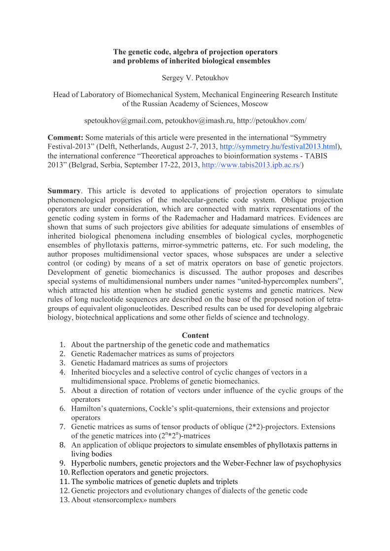
Figure 3. The illustration of cyclic groups of operators on the basis of sums of projection operators (c0+c1) and (c2+c3) from Figure 2 in cases of their exponentiation.

These two sums of column projectors (c0+c1) and (c2+c3) are marked by green colour in the left table on Figure 4, where every of cells represents a sum of those projectors, which denote its column and row.

Two other examined sums of column projectors (c0+c2) and (c1+c3) is doubled when squaring: (c0+c2)n = 2n-1*(c0+c2), (c1+c3)n = 2n-1*(c1+c3), where n = 1, 2, 3,… (these sums are marked by red colours in the left table on Figure 4) . This doubling reminds dichotomic dividing of biological cells in a result of mitosis when doubling of genetic information occurs.

The last examined sums of the column projectors (c0+c3) and (c1+c2) possess the following feature. Matrices of their second power is quadrupled in a result of exponentiation in integer powers: ((c0+c3)2)n = 4n-1*(c0+c3)2, ((c1+c2)2)n = 4n-1*(c1+c2)2, where n = 1, 2, 3… (this feature can be used to simulate a genetic phenomenon of tetra-reproduction of gametes and genetic information in a course of meiosis). The cells with these sums (c0+c3) and (c1+c2) are marked by yellow colour in the left table on Figure 4.

If we examine the row projectors r0, r1, r2 and r3 from Figure 2, we receive the same tabular structure with a small change: red and yellow cells are swapped (Figure 4, right). Matrices 2-0.5*(r0+r1) and 2-0.5*(r2+r3) are basises for cyclic groups with a period 8 in relation to their exponentiation (green cells in the right table on Figure 4). Matrices (r0+r2) and (r1+r3) is doubled when squaring: (r0+r2)n = 2n-1*(r0+r2), (r1+r3)n = 2n-1*(r1+r3), where n = 1, 2, 3,… (red cells in the right table on Figure 4). Matrices (r0+r3) and (r1+r2) possess the «quadruplet» property: ((r0+r3)2)n = 4n-1*(r0+r3)2, ((r1+r2)2)n = 4n-1*(r1+r2)2, where n = 1, 2, 3… (yellow cells in the right table on Figure 4). The cells on the main diagonal correspond to sum of two projectors themselves: (ci+ci)n = 2n*ci, (ri+ri)n = 2n*ri, where i = 0, 1, 2, 3.

c0 c1 c2 c3

c0 - c0+c1 c0+c2 c0+c3 c1 c1+c0 - c1+c2 c1+c3 c2 c2+c0 c2+c1 - c2+c3 c3 c3+c0 c3+c1 c3+c2 -

r0 r1 r2 r3

r0 - r0+r1 r0+r2 r0+r3 r1 r1+r0 - r1+r2 r1+r3 r2 r2+r0 r2+r1 - r2+r3 r3 r3+r0 r3+r1 r3+r2 -

Figure 4. Tables of some features of sums of pairs of different «column projectors» c0, c1, c2, c3 and of «row projectors» r0, r1, r2, r3 (from the Rademacher matrix R4 on Figure 2) in relation to their exponentiation. Explanations in text.

One can mention that the structure of this symmetric table is unexpectedly coincided with the structure of the typical (4*4)-matrix of dyadic shifts, which is known in theory of

signal processing and which is related with some phenomenologic properties of molecular-genetic systems [Ahmed, Rao, 1975; Petoukhov, 2008, 2012a; Petoukhov, He, 2009].

It should be noted that cyclic features of (4*4)-matrices 2-0.5*(c0+c1), 2-0.5*(c2+c3), 2-

0.5*(r0+r1) and 2-0.5*(r2+r3) in cases of their exponentiation exist due to their connections with matrix representations of 2-parametric complex numbers in 4-dimensional space; these connections are shown by means of a new decomposition of each of these matrices into sum of new sparse matrices e0 and e1 (Figures 5, 6, two upper levels, where the multiplication table for e0 and e1 in the right column is identical to the multiplication table of complex numbers). The dichotomic features of (4*4)-matrices (c0+c2), (c1+c3), (r0+r3), (r1+r2) and tetra-reproduction features of (4*4)-matrices ((c0+c3)2)n = 4n-1*(c0+c3)2, ((c1+c2)2)n = 4n-

1*(c1+c2)2, ((r0+r2)2)n = 4n-1*(r0+r2)2, ((r1+r3)2)n = 4n-1*(r1+r3)2 exist due to their connections with matrix representations of 2-parametric hyperbolic numbers in 4-dimensional space (Figures 5, 6, four bottom levels, where the multiplication table for e0 and e1 in the right column is identical to the multiplication table of hyperbolic numbers). Synonyms of hyperbolic numbers are Lorentz numbers, split-complex numbers, double numbers, perplex numbers, etc. - http://en.wikipedia.org/wiki/Split-complex_number). Hyperbolic numbers are a two-dimensional commutative algebra over the real numbers. Additional details about such (4*4)-matrix representations of complex numbers and hyperbolic numbers see in [Petoukhov, 2012b].

c0+с1 =

1 1 0 0 -1 1 0 0 1 -1 0 0 -1 -1 0 0

= e0+e1 =

1 0 0 0 0 1 0 0 0 -1 0 0 -1 0 0 0

+

0 1 0 0 -1 0 0 0 1 0 0 0 0 -1 0 0

e0 e1 ; e0 e0 e1 e1 e1 -e0

c2+c3 =

0 0 1 -1 0 0 -1 -1 0 0 1 1 0 0 -1 1

= e0+e1 =

0 0 0 -1 0 0 -1 0 0 0 1 0 0 0 0 1

+

0 0 1 0 0 0 0 -1 0 0 0 1 0 0 -1 0

e0 e1 ; e0 e0 e1 e1 e1 -e0

c0+c2=

1 0 1 0 -1 0 -1 0 1 0 1 0 -1 0 -1 0

= e0+e1 =

1 0 0 0 -1 0 0 0 0 0 1 0 0 0 -1 0

+

0 0 1 0 0 0 -1 0 1 0 0 0 -1 0 0 0

e0 e1 ; e0 e0 e1 e1 e1 e0

c1+c3 =

0 1 0 -1 0 1 0 -1 0 -1 0 1 0 -1 0 1

= e0+e1 =

0 1 0 0 0 1 0 0 0 0 0 1 0 0 0 1

+

0 0 0 -1 0 0 0 -1 0 -1 0 0 0 -1 0 0

e0 e1 ; e0 e0 e1 e1 e1 e0

0.5*(c0+c3)2 =

1 0 0 -1 0 0 0 0 0 0 0 0 -1 0 0 1

= e0+e1 =

1 0 0 0 0 0 0 0 0 0 0 0 0 0 0 1

+

0 0 0 -1 0 0 0 0 0 0 0 0 -1 0 0 0

e0 e1 ; e0 e0 e1 e1 e1 e0

0.5*(c1+c2)2 =

0 0 0 0 0 1 -1 0 0 -1 1 0 0 0 0 0

= e0+e1=

0 0 0 0 0 1 0 0 0 0 1 0 0 0 0 0

+

0 0 0 0 0 0 -1 0 0 -1 0 0 0 0 0 0

e0 e1 ; e0 e0 e1 e1 e1 e0

Figure 5. The table represents special decompositions of (4*4)-matrices (c0+c1), (c2+c3), (c0+c2), (c1+c3), 0.5*(c0+c3)2 and 0.5*(c1+c2)2 into sum of two matrices e0+e1 (see also Figures 2 and 4). The table shows direct relations of these matrices with matrix representations of 2-parametric complex numbers and hyperbolic numbers. Here c0, c1, c2 and c3 are column projectors from Figure 2. For each set of matrices e0 and e1 at every tabular level, the right column of this table contains its multiplication table: for two upper levels it is a known multiplication table of complex numbers; for other four levels it is a known multiplication table of hyperbolic numbers.

r0+r1 =

1 1 1 -1 -1 1 -1 -1 0 0 0 0 0 0 0 0

= e0+e1=

1 0 1 0 0 1 0 -1 0 0 0 0 0 0 0 0

+

0 1 0 -1 -1 0 -1 0 0 0 0 0 0 0 0 0

e0 e1 ; e0 e0 e1 e1 e1 -e0

r2+r3 =

0 0 0 0 0 0 0 0 1 -1 1 1 -1 -1 -1 1

= e0+e1=

0 0 0 0 0 0 0 0 1 0 1 0 0 -1 0 1

+

0 0 0 0 0 0 0 0 0 -1 0 1 -1 0 -1 0

e0 e1 ; e0 e0 e1 e1 e1 -e0

0.5*(r0+r2)2=

1 0 1 0 0 0 0 0 1 0 1 0 0 0 0 0

= e0+e1=

1 0 0 0 0 0 0 0 0 0 1 0 0 0 0 0

+

0 0 1 0 0 0 0 0 1 0 0 0 0 0 0 0

e0 e1 ; e0 e0 e1 e1 e1 e0

0.5*(r1+r3)2=

0 0 0 0 0 1 0 -1 0 0 0 0 0 -1 0 1

= e0+e1=

0 0 0 0 0 1 0 0 0 0 0 0 0 0 0 1

+

0 0 0 0 0 0 0 -1 0 0 0 0 0 -1 0 0

e0 e1 ; e0 e0 e1 e1 e1 e0

r0+r3 =

1 1 1 -1 0 0 0 0 0 0 0 0 -1 -1 -1 1

= e0+e1=

1 1 0 0 0 0 0 0 0 0 0 0 0 0 -1 1

0 0 1 -1 0 0 0 0 0 0 0 0 -1 -1 0 0

e0 e1 ; e0 e0 e1 e1 e1 e0

r1+r2 =

0 0 0 0 -1 1 -1 -1 1 -1 1 1 0 0 0 0

= e0+e1=

0 0 0 0 -1 1 0 0 0 0 1 1 0 0 0 0

+

0 0 0 0 0 0 -1 -1 1 -1 0 0 0 0 0 0

e0 e1 ; e0 e0 e1 e1 e1 e0

Figure 6. The table represents special decompositions of (4*4)-matrices (r0+r1), (r2+r3), 0.5*(r0+r2)2, 0.5*(r1+r3)2, (r0+r3) and (r1+r2) into sum of two matrices e0+e1. The table shows direct relations of these matrices with matrix representations of 2-parametric complex numbers and hyperbolic numbers. Here r0, r1, r2 and r3 are row projectors from Figure 2. For each set of matrices e0 and e1 at every tabular level, the right column of this table contains its multiplication table: for two upper levels it is a known multiplication table of complex

numbers; for other four levels it is a known multiplication table of hyperbolic numbers.

Now let us turn to the Rademacher (8*8)-matrix R8 (Figure 1) to analyze its column decomposition R8 = s0+s1+s2+s3+s4+s5+s6+s7 (Fugure 7) and its row decomposition R8 = v0+v1+v2+v3+v4+v5+v6+v7 (Figure 8).

Figure 7. The «column decomposition» R8 = s0+s1+s2+s3+s4+s5+s6+s7 of the Rademacher (8*8)-matrix R8 (Figure 1) where every of matrices s0, s1, s2, s3, s4, s5, s6, s7 is a projection operator

R8 = s0+s1+s2+s3+ s4+s5+s6+s7 =

1 0 0 0 0 0 0 0 1 0 0 0 0 0 0 0 -1 0 0 0 0 0 0 0 -1 0 0 0 0 0 0 0 1 0 0 0 0 0 0 0 1 0 0 0 0 0 0 0 -1 0 0 0 0 0 0 0 -1 0 0 0 0 0 0 0

+

0 1 0 0 0 0 0 0 0 1 0 0 0 0 0 0 0 -1 0 0 0 0 0 0 0 -1 0 0 0 0 0 0 0 1 0 0 0 0 0 0 0 1 0 0 0 0 0 0 0 -1 0 0 0 0 0 0 0 -1 0 0 0 0 0 0

+

0 0 1 0 0 0 0 0 0 0 1 0 0 0 0 0 0 0 1 0 0 0 0 0 0 0 1 0 0 0 0 0 0 0 -1 0 0 0 0 0 0 0 -1 0 0 0 0 0 0 0 -1 0 0 0 0 0 0 0 -1 0 0 0 0 0

+

0 0 0 1 0 0 0 0 0 0 0 1 0 0 0 0 0 0 0 1 0 0 0 0 0 0 0 1 0 0 0 0 0 0 0 -1 0 0 0 0 0 0 0 -1 0 0 0 0 0 0 0 -1 0 0 0 0 0 0 0 -1 0 0 0 0

+

0 0 0 0 1 0 0 0 0 0 0 0 1 0 0 0 0 0 0 0 -1 0 0 0 0 0 0 0 -1 0 0 0 0 0 0 0 1 0 0 0 0 0 0 0 1 0 0 0 0 0 0 0 -1 0 0 0 0 0 0 0 -1 0 0 0

+

0 0 0 0 0 1 0 0 0 0 0 0 0 1 0 0 0 0 0 0 0 -1 0 0 0 0 0 0 0 -1 0 0 0 0 0 0 0 1 0 0 0 0 0 0 0 1 0 0 0 0 0 0 0 -1 0 0 0 0 0 0 0 -1 0 0

+

0 0 0 0 0 0 -1 0 0 0 0 0 0 0 -1 0 0 0 0 0 0 0 -1 0 0 0 0 0 0 0 -1 0 0 0 0 0 0 0 1 0 0 0 0 0 0 0 1 0 0 0 0 0 0 0 1 0 0 0 0 0 0 0 1 0

+

0 0 0 0 0 0 0 -1 0 0 0 0 0 0 0 -1 0 0 0 0 0 0 0 -1 0 0 0 0 0 0 0 -1 0 0 0 0 0 0 0 1 0 0 0 0 0 0 0 1 0 0 0 0 0 0 0 1 0 0 0 0 0 0 0 1

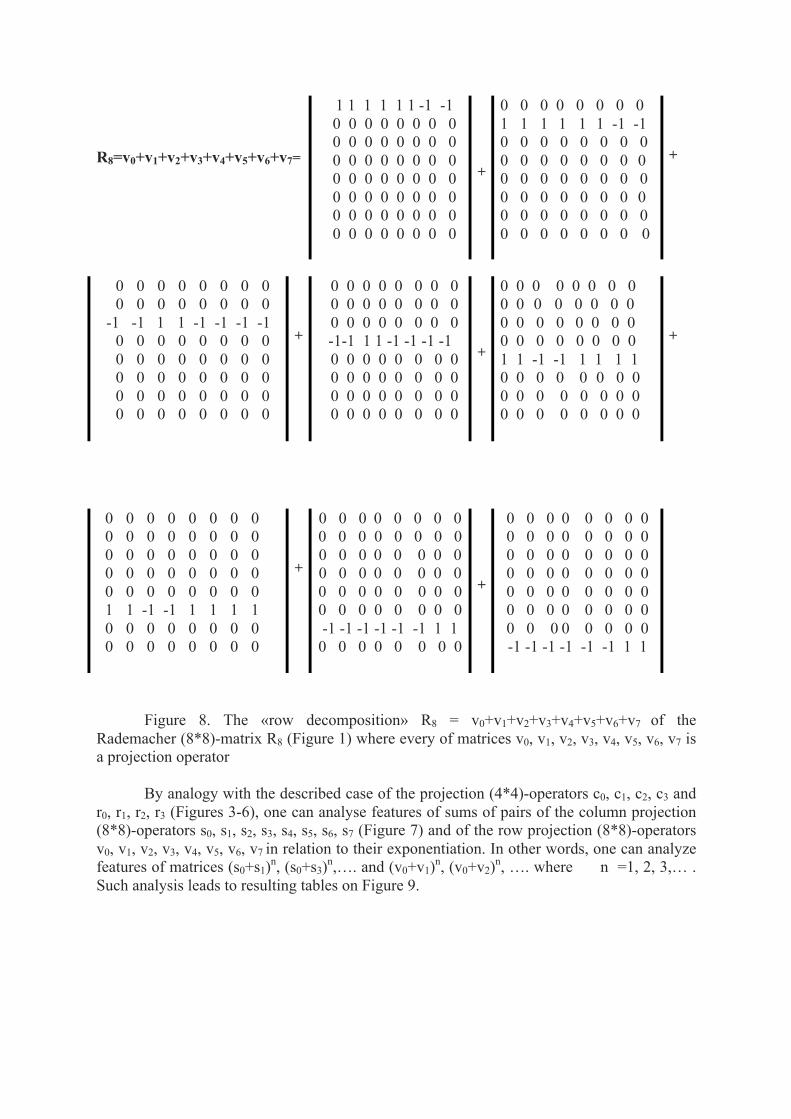
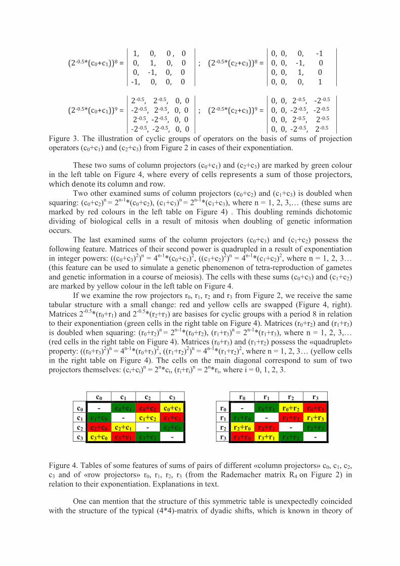
Figure 8. The «row decomposition» R8 = v0+v1+v2+v3+v4+v5+v6+v7 of the Rademacher (8*8)-matrix R8 (Figure 1) where every of matrices v0, v1, v2, v3, v4, v5, v6, v7 is a projection operator

By analogy with the described case of the projection (4*4)-operators c0, c1, c2, c3 and r0, r1, r2, r3 (Figures 3-6), one can analyse features of sums of pairs of the column projection (8*8)-operators s0, s1, s2, s3, s4, s5, s6, s7 (Figure 7) and of the row projection (8*8)-operators v0, v1, v2, v3, v4, v5, v6, v7 in relation to their exponentiation. In other words, one can analyze features of matrices (s0+s1)n, (s0+s3)n,…. and (v0+v1)n, (v0+v2)n, …. where n =1, 2, 3,… . Such analysis leads to resulting tables on Figure 9.

R8=v0+v1+v2+v3+v4+v5+v6+v7=

1 1 1 1 1 1 -1 -1 0 0 0 0 0 0 0 0 0 0 0 0 0 0 0 0 0 0 0 0 0 0 0 0 0 0 0 0 0 0 0 0 0 0 0 0 0 0 0 0 0 0 0 0 0 0 0 0 0 0 0 0 0 0 0 0

+

0 0 0 0 0 0 0 0 1 1 1 1 1 1 -1 -1 0 0 0 0 0 0 0 0 0 0 0 0 0 0 0 0 0 0 0 0 0 0 0 0 0 0 0 0 0 0 0 0 0 0 0 0 0 0 0 0 0 0 0 0 0 0 0 0

+

0 0 0 0 0 0 0 0 0 0 0 0 0 0 0 0

-1 -1 1 1 -1 -1 -1 -1 0 0 0 0 0 0 0 0 0 0 0 0 0 0 0 0 0 0 0 0 0 0 0 0 0 0 0 0 0 0 0 0 0 0 0 0 0 0 0 0

+

0 0 0 0 0 0 0 0 0 0 0 0 0 0 0 0 0 0 0 0 0 0 0 0 -1-1 1 1 -1 -1 -1 -1 0 0 0 0 0 0 0 0 0 0 0 0 0 0 0 0 0 0 0 0 0 0 0 0 0 0 0 0 0 0 0 0

+

0 0 0 0 0 0 0 0 0 0 0 0 0 0 0 0 0 0 0 0 0 0 0 0 0 0 0 0 0 0 0 0 1 1 -1 -1 1 1 1 1 0 0 0 0 0 0 0 0 0 0 0 0 0 0 0 0 0 0 0 0 0 0 0 0

+

0 0 0 0 0 0 0 0 0 0 0 0 0 0 0 0 0 0 0 0 0 0 0 0 0 0 0 0 0 0 0 0 0 0 0 0 0 0 0 0 1 1 -1 -1 1 1 1 1 0 0 0 0 0 0 0 0 0 0 0 0 0 0 0 0

+

0 0 0 0 0 0 0 0 0 0 0 0 0 0 0 0 0 0 0 0 0 0 0 0 0 0 0 0 0 0 0 0 0 0 0 0 0 0 0 0 0 0 0 0 0 0 0 0 -1 -1 -1 -1 -1 -1 1 1

0 0 0 0 0 0 0 0

+

0 0 0 0 0 0 0 0 0 0 0 0 0 0 0 0 0 0 0 0 0 0 0 0 0 0 0 0 0 0 0 0 0 0 0 0 0 0 0 0 0 0 0 0 0 0 0 0 0 0 0 0 0 0 0 0 -1 -1 -1 -1 -1 -1 1 1

s0 s1 s2 s3 s4 s5 s6 s7 s0 - s1 - s2 - s3 - s4 - s5 - s6 - s7 -

v0 v1 v2 v3 v4 v5 v6 v7 v0 - v1 - v2 - v3 - v4 - v5 - v6 - v7 -

Figure 9. Tables of some features of sums of pairs of different column projectors s0, s1, …, s7 (from Figure 7) and of row projectors v0, v1, …, v7 (from the Rademacher matrix R8 on Figure 8) in relation to their exponentiation. Explanations in text.

Every of cells in these tables on Figure 9 represents a sum of those projectors which

denote its column and row by analogy with Figure 4. Again we have three types of such sums which are marked by green, red and yellow and which possess the similar properties in comparison with the cases on Figure 4.

In each of tables on Figure 9, green cells correspond to those matrices, exponentiations of which generate 8 cyclic groups. The left table contains 16 green cells that correspond to the following cyclic groups with a period 8: (2-0.5*(s0+s2))n, (2-0.5*(s0+s3))n, (2-0.5*(s1+s2))n, (2-0.5*(s1+s3))n, (2-0.5*(s4+s6))n, (2-0.5*(s4+s7))n, (2-0.5*(s5+s6))n, (2-0.5*(s5+s7))n. The right table contains 16 green cells with the same tabular location that correspond to the following cyclic groups with a period 8: (2-0.5*(v0+v2))n, (2-0.5*(v0+v3))n, (2-0.5*(v1+v2))n, (2-0.5*(v1+v3))n, (2-0.5*(v4+v6))n, (2-0.5*(v4+v7))n, (2-0.5*( v5+v6))n, (2-0.5*(v5+v7))n.

Red cells in tables on Figure 9 contain those matrices which possess a doubling property in relation to their exponentiation. The left table contains 24 red cells, matrices of which satisfy the following feature: (s0+s1)n = 2n-1*(s0+s1), (s0+s4)n = 2n-1*(s0+s4), etc. The right table also contains 24 red cells with the same feature but with another tabular location: (v0+v1)n = 2n-1*(v0+v1), (v0+v4)n = 2n-1*(v0+v4), etc.

16 yellow cells in each of tables on Figure 9 contain those matrices, which have «quadruplet property»: ((s0+s6)2)n = 4n-1*(s0+s6)2, ((v0+v4)2)n = 4n-1*(v0+v4)2, etc. The cells on the main diagonal correspond to sum of two projectors themselves: (si+si)n = 2n*si, (vi+vi)n = 2n*vi, where i = 0, 1, 2, ..., 7.

3. GENETIC HADAMARD MATRICES AS SUMS OF PROJECTORS

The genetic Hadamard matrix H4 from Figure 1 can be also decomposed into sum of 4 sparse matrices H4 = h0+h1+h2+h3 where each of sparse matrices contains only one non-zero column (in a case of the «column decomposition») or only one non-zero row (in a case of the «row decomposition») (Figure 10).

H4 = h0+h1+h2+h3 =

1 0 0 0 -‐1 0 0 0 1 0 0 0 -‐1 0 0 0

+

0 1 0 0 0 1 0 0 0 -‐1 0 0 0 -‐1 0 0

+

0 0 -‐1 0 0 0 1 0 0 0 1 0 0 0 -‐1 0

+

0 0 0 1 0 0 0 1 0 0 0 1 0 0 0 1

H4 = g0+g1+g2+g3 =

1 1 -1 1 0 0 0 0 0 0 0 0 0 0 0 0

+

0 0 0 0 -1 1 1 1 0 0 0 0 0 0 0 0

+

0 0 0 0 0 0 0 0 1 -1 1 1 0 0 0 0

+

0 0 0 0 0 0 0 0 0 0 0 0 -1 -1 -1 1

Figure 10. The «column decomposition» (upper layer) and the «row decomposition» (bottom layer) of the Hadamard matrix H4 from Figure 1

Each of these sparse matrices h0, h1, h2, h3 and g0, g1, g2, g3 on Fugure 10 is a projector. We will conditionally name projectors h0, h1, h2, h3 again as «column projectors» and projectors g0, g1, g2, g3 as «row projectors».

By analogy with the previous section about the Rademacher matrix R4, one can analyse features of sums of pairs of these column projectors and row projectors in relation to their exponentiation. In other words, one can analyze features of matrices (h0+h1)n, (h0+h2)n,…. and (g0+g1)n, (g0+g2)n, …. where n =1, 2, 3,… . Such analysis leads to resulting tables on Figure 11.

h0 h1 h2 h3 h0 - h1 - h2 - h3 -

g0 g1 g2 g3 g0 - g1 - g2 - g3 -

Figure 11. Tables of some features of sums of pairs of the different «column projectors» h0, h1, h2, h3 (in the left table) and of the «row projectors» g0, g1, g2, g3 (from the Hadamard matrix H4 on Figure 10) in relation to their exponentiation. Explanations in text.

Both tables on Figure 11 are identical in their mosaics. Every of their cells correspond to a sum of those column projectors (or row projectors), which denote its column and row. 12 green cells correspond to matrices, exponentiations of which lead to cyclic groups with a period 8: (2-0.5*(h0+h1))n, (2-0.5*(h0+h2))n, … , (2-0.5*(g0+g1))n, (2-0.5*(g0+g1))n, … , where n = 1, 2, 3,… . The cells on the main diagonal correspond to sum of two projectors themselves: (hi+hi)n = 2n*hi, (gi+gi)n = 2n*gi, where i = 0, 1, 2, 3.

Cyclic properties of these (4*4)-matrix operators exist due to a connection of these operators with complex numbers. Figures 12 and 13 show existence of a special decomposition of every of these (4*4)-matrices into such set of two sparse matrices e0 and e1, which is closed relative to multiplication and which defines their multiplication table that coincides with the known multiplication table of complex numbers.

h0+h1 =

1 1 0 0 -1 1 0 0 1 -1 0 0 -1 -1 0 0

= e0+e1=

1 0 0 0 0 1 0 0 0 -1 0 0 -1 0 0 0

+

0 1 0 0 -1 0 0 0 1 0 0 0 0 -1 0 0

;

e0 e1

e0 e0 e1

e1 e1 -e0

h0+h2 =

1 0 -1 0 -1 0 1 0 1 0 1 0 -1 0 -1 0

= e0+e1=

1 0 0 0 -1 0 0 0 0 0 1 0 0 0 -1 0

+

0 0 -1 0 0 0 1 0 1 0 0 0 -1 0 0 0

;

e0 e1

e0 e0 e1

e1 e1 -e0

h0+h3 =

1 0 0 1 -1 0 0 1 1 0 0 1 -1 0 0 1

= e0+e1=

1 0 0 0 0 0 0 1 1 0 0 0 0 0 0 1

+

0 0 0 1 -1 0 0 0 0 0 0 1 -1 0 0 0

;

e0 e1

e0 e0 e1

e1 e1 -e0

h1+h2 =

0 1 -1 0 0 1 1 0 0 -1 1 0 0 -1 -1 0

= e0+e1=

0 0 -1 0 0 1 0 0 0 0 1 0 0 -1 0 0

+

0 1 0 0 0 0 1 0 0 -1 0 0 0 0 -1 0

;

e0 e1

e0 e0 e1

e1 e1 -e0

h1+h3 =

0 1 0 1 0 1 0 1 0 -1 0 1 0 -1 0 1

= e0+e1=

0 1 0 0 0 1 0 0 0 0 0 1 0 0 0 1

+

0 0 0 1 0 0 0 1 0 -1 0 0 0 -1 0 0

;

e0 e1

e0 e0 e1

e1 e1 -e0

h2+h3 =

0 0 -1 1 0 0 1 1 0 0 1 1 0 0 -1 1

= e0+e1=

0 0 0 1 0 0 1 0 0 0 1 0 0 0 0 1

+

0 0 -1 0 0 0 0 1 0 0 0 1 0 0 -1 0

;

e0 e1

e0 e0 e1

e1 e1 -e0

Figure 12. The table represents special decompositions of (4*4)-matrices (h0+h1), (h0+h2), (h0+h3), (h1+h2), (h1+h3), (h2+h3) into sum of two matrices e0+e1. The table shows direct relations of these matrices with matrix representations of 2-parametric complex numbers. Here h0, h1, h2 and h3 are column projectors of the Hadamard matrix H4 from Figure 10. For each set of matrices e0 and e1 at every tabular level, the right column of the table contains its multiplication table, which coinsides with the multiplication table of complex numbers.

g0+g1 =

1 1 -1 1 -1 1 1 1 0 0 0 0 0 0 0 0

= e0+e1 =

1 0 -1 0 0 1 0 1 0 0 0 0 0 0 0 0

+

0 1 0 1 -1 0 1 0 0 0 0 0 0 0 0 0

;

e0 e1

e0 e0 e1

e1 e1 -e0

g0+g2 =

1 1 -1 1 0 0 0 0 1 -1 1 1 0 0 0 0

= e0+e1 =

1 0 0 1 0 0 0 0 0 -1 1 0 0 0 0 0

+

0 1 -1 0 0 0 0 0 1 0 0 1 0 0 0 0

;

e0 e1

e0 e0 e1

e1 e1 -e0

g0+g3 =

1 1 -1 1 0 0 0 0 0 0 0 0 -1 -1 -1 1

= e0+e1 =

1 1 0 0 0 0 0 0 0 0 0 0 0 0 -1 1

+

0 0 -1 1 0 0 0 0 0 0 0 0 -1 -1 0 0

;

e0 e1

e0 e0 e1

e1 e1 -e0

g1+g2 =

0 0 0 0 -1 1 1 1 1 -1 1 1 0 0 0 0

= e0+e1 =

0 0 0 0 -1 1 0 0 0 0 1 1 0 0 0 0

+

0 0 0 0 0 0 1 1 1 -1 0 0 0 0 0 0

;

e0 e1

e0 e0 e1

e1 e1 -e0

g1+g3 =

0 0 0 0 -1 1 1 1 0 0 0 0 -1 -1 -1 1

= e0+e1 =

0 0 0 0 0 1 1 0 0 0 0 0 -1 0 0 1

+

0 0 0 0 -1 0 0 1 0 0 0 0 0 -1 -1 0

;

e0 e1

e0 e0 e1

e1 e1 -e0

g2+g3 =

0 0 0 0 0 0 0 0 1 -1 1 1 -1 -1 -1 1

= e0+e1 =

0 0 0 0 0 0 0 0 1 0 1 0 0 -1 0 1

+

0 0 0 0 0 0 0 0 0 -1 0 1 -1 0 -1 0

;

e0 e1

e0 e0 e1

e1 e1 -e0

Fugure 13. The table represents special decompositions of (4*4)-matrices (g0+g1), (g0+g2), (g0+g3), (g1+g2), (g1+g3), (g2+g3) into sum of two matrices e0+e1. The table shows direct relations of these matrices with matrix representations of 2-parametric complex numbers. Here g0, g1, g2 and g3 are row projectors from Figure 10. For each set of matrices e0 and e1 at every tabular level, the right column of the table contains its multiplication table, which coinsides with the multiplication table of complex numbers.

Now let us turn to the genetic Hadamard matrix H8 from Figure 1. It can be also decomposed into sum of 8 sparse matrices H8=u0+u1+u2+u3+u4+u5+u6+u7 where each of sparse matrices contains only one non-zero column (in a case of the «column decomposition») or only one non-zero row (in a case of the «row decomposition») (Figure 14).

H8=u0+u1+u2+ u3+u4+u5+u6+u7

=

1 0 0 0 0 0 0 0 1 0 0 0 0 0 0 0 -1 0 0 0 0 0 0 0 -1 0 0 0 0 0 0 0 1 0 0 0 0 0 0 0 1 0 0 0 0 0 0 0 -1 0 0 0 0 0 0 0 -1 0 0 0 0 0 0 0

+

0 -1 0 0 0 0 0 0 0 1 0 0 0 0 0 0 0 1 0 0 0 0 0 0 0 -1 0 0 0 0 0 0 0 -1 0 0 0 0 0 0 0 1 0 0 0 0 0 0 0 1 0 0 0 0 0 0 0 -1 0 0 0 0 0 0

+

Figure 14. The «column decomposition» H8=u0+u1+u2+u3+u4+u5+u6+u7 of the Hadamard (8*8)-matrix H8 (Figure 1) where every of sparse matrices u0, u1, u2, u3, u4, u5, u6, u7 is a projection operator

H8=d0+d1+d2+d3+ d4+d5+d6+d7

=

1 -1 1 -1 -1 1 1 -1 0 0 0 0 0 0 0 0 0 0 0 0 0 0 0 0 0 0 0 0 0 0 0 0 0 0 0 0 0 0 0 0 0 0 0 0 0 0 0 0 0 0 0 0 0 0 0 0 0 0 0 0 0 0 0 0

+

0 0 0 0 0 0 0 0 1 1 1 1 -1 -1 1 1 0 0 0 0 0 0 0 0 0 0 0 0 0 0 0 0 0 0 0 0 0 0 0 0 0 0 0 0 0 0 0 0 0 0 0 0 0 0 0 0 0 0 0 0 0 0 0 0

0 0 0 0 0 0 0 0 0 0 0 0 0 0 0 0 -1 1 1 -1 1 -1 1 -1 0 0 0 0 0 0 0 0 0 0 0 0 0 0 0 0 0 0 0 0 0 0 0 0 0 0 0 0 0 0 0 0 0 0 0 0 0 0 0 0

+

0 0 0 0 0 0 0 0 0 0 0 0 0 0 0 0 0 0 0 0 0 0 0 0 -1 -1 1 1 1 1 1 1 0 0 0 0 0 0 0 0 0 0 0 0 0 0 0 0 0 0 0 0 0 0 0 0 0 0 0 0 0 0 0 0

+

0 0 0 0 0 0 0 0 0 0 0 0 0 0 0 0 0 0 0 0 0 0 0 0 0 0 0 0 0 0 0 0 1 -1 -1 1 1 -1 1 -1 0 0 0 0 0 0 0 0 0 0 0 0 0 0 0 0 0 0 0 0 0 0 0 0

0 0 1 0 0 0 0 0 0 0 1 0 0 0 0 0 0 0 1 0 0 0 0 0 0 0 1 0 0 0 0 0 0 0 -1 0 0 0 0 0 0 0 -1 0 0 0 0 0 0 0 -1 0 0 0 0 0 0 0 -1 0 0 0 0 0

+

0 0 0 -1 0 0 0 0 0 0 0 1 0 0 0 0 0 0 0 -1 0 0 0 0 0 0 0 1 0 0 0 0 0 0 0 1 0 0 0 0 0 0 0 -1 0 0 0 0 0 0 0 1 0 0 0 0 0 0 0 -1 0 0 0 0

+

0 0 0 0 -1 0 0 0 0 0 0 0 -1 0 0 0 0 0 0 0 1 0 0 0 0 0 0 0 1 0 0 0 0 0 0 0 1 0 0 0 0 0 0 0 1 0 0 0 0 0 0 0 -1 0 0 0 0 0 0 0 -1 0 0 0

+

0 0 0 0 0 1 0 0 0 0 0 0 0 -1 0 0 0 0 0 0 0 -1 0 0 0 0 0 0 0 1 0 0 0 0 0 0 0 -1 0 0 0 0 0 0 0 1 0 0 0 0 0 0 0 1 0 0 0 0 0 0 0 -1 0 0

+

0 0 0 0 0 0 1 0 0 0 0 0 0 0 1 0 0 0 0 0 0 0 1 0 0 0 0 0 0 0 1 0 0 0 0 0 0 0 1 0 0 0 0 0 0 0 1 0 0 0 0 0 0 0 1 0 0 0 0 0 0 0 1 0

+

0 0 0 0 0 0 0 -1 0 0 0 0 0 0 0 1 0 0 0 0 0 0 0 -1 0 0 0 0 0 0 0 1 0 0 0 0 0 0 0 -1 0 0 0 0 0 0 0 1 0 0 0 0 0 0 0 -1 0 0 0 0 0 0 0 1

0 0 0 0 0 0 0 0 0 0 0 0 0 0 0 0 0 0 0 0 0 0 0 0 0 0 0 0 0 0 0 0 0 0 0 0 0 0 0 0 1 1 -1 -1 1 1 1 1 0 0 0 0 0 0 0 0 0 0 0 0 0 0 0 0

+

0 0 0 0 0 0 0 0 0 0 0 0 0 0 0 0 0 0 0 0 0 0 0 0 0 0 0 0 0 0 0 0 0 0 0 0 0 0 0 0 0 0 0 0 0 0 0 0 -1 1 -1 1 -1 1 1 -1 0 0 0 0 0 0 0 0

+

0 0 0 0 0 0 0 0 0 0 0 0 0 0 0 0 0 0 0 0 0 0 0 0 0 0 0 0 0 0 0 0 0 0 0 0 0 0 0 0 0 0 0 0 0 0 0 0 0 0 0 0 0 0 0 0 -1 -1 -1 -1 -1 -1 1 1

Figure 15. The «row decomposition» H8=d0+d1+d2+d3+d4+d5+d6+d7 of the Hadamard (8*8)-‐matrix H8 (Figure 1) where every of sparse matrices d0, d1, d2, d3, d4, d5, d6, d7 is a projection operator

Every of these sparse matrices u0, u1, u2, u3, u4, u5, u6, u7 and d0, d1, d2, d3, d4, d5, d6, d7 on Fugures 14, 15 is a projector. We will conditionally name projectors u0, u1, u2, u3, u4, u5, u6, u7 again as «column projectors» and projectors d0, d1, d2, d3, d4, d5, d6, d7 as «row projectors».

By analogy with the previous sections, one can analyse features of sums of pairs of these column projectors and row projectors in relation to their exponentiation. In other words, one can analyze features of matrices (u0+u1)n, (u0+u3)n,…. and (d0+d1)n, (d0+d2)n, …. where n =1, 2, 3,… . Such analysis leads to resulting tables on Figure 16.

u0 u1 u2 u3 u4 u5 u6 u7 u0 - u1 - u2 - u3 - u4 - u5 - u6 - u7 -

d0 d1 d2 d3 d4 d5 d6 d7

d0 - d1 - d2 - d3 - d4 - d5 - d6 - d7 -

Figure 16. Tables of some features of sums of pairs of the different column projectors u0, u1, …, u7 (from Figure 14) and of the row projectors d0, d1, …, d7 (from Figure 15) in relation to their exponentiation. This is the case of the Hadamard matrix H8 from Figure 1. Explanations in text.

Both tables on Figure 16 have the identical mosaic with 32 green cells and 24 yellow cells. The green cells in these tables correspond to those matrices, exponentiations of which generate cyclic groups with a period 8:

• (2-0.5*(u0+u1))n, (2-0.5*(u0+u2))n, (2-0.5*(u0+u4))n, (2-0.5*(u0+u6))n, (2-0.5*(u1+u3))n, (2-0.5*(u1+u5))n, (2-0.5*(u1+u7))n, (2-0.5*(u2+u3))n, (2-0.5*(u2+u4))n, (2-0.5*(u2+u6))n, (2-0.5*(u3+u5))n, (2-0.5*(u3+u7))n, (2-0.5*(u4+u5))n, (2-0.5*(u4+u6))n, (2-0.5*(u5+u7))n, (2-0.5*(u6+u7))n (in the left table);

• (2-0.5*(d0+d1))n, (2-0.5*(d0+d2))n, (2-0.5*(d0+d4))n, (2-0.5*(d0+d6))n, (2-0.5*(d1+d3))n, (2-0.5*(d1+d5))n, (2-0.5*(d1+d7))n, (2-0.5*(d2+d3))n, (2-0.5*(d2+d4))n, (2-0.5*(d2+d6))n, (2-0.5*(d3+d5))n, (2-0.5*(d3+d7))n, (2-0.5*(d4+d5))n, (2-0.5*(d4+d6))n, (2-0.5*(d5+d7))n, (2-0.5*(d6+d7))n (in the right table).

Cyclic properties of these (8*8)-matrix operators exist due to a connection of these operators with complex numbers. Figure 17 shows some examples of decompositions of the (8*8)-matrices from green cells on Figure 16 into corresponding sets of two sparse matrices, each of which is closed in relation to multiplication and each of which defines the multiplication table of complex numbers (see some additional details about representations of complex numbers by means of (2n*2n)-matrices in [Petoukhov, 2012b]). It should be noted here that our study in the field of matrix genetics has revealed methods of extension of these (8*8)-genetic matrices R4, R8, H4, H8 (Figure 1) into (2n*2n)-matrices which are also sums of "column projectors" and "row projectors" and which give by analogy as much cyclic groups as needed to model big ensembles of cyclic processes.

u0+u4 =

1 0 0 0 -1 0 0 0 1 0 0 0 -1 0 0 0 -1 0 0 0 1 0 0 0 -1 0 0 0 1 0 0 0 1 0 0 0 1 0 0 0 1 0 0 0 1 0 0 0 -1 0 0 0 -1 0 0 0 -1 0 0 0 -1 0 0 0

=

1 0 0 0 0 0 0 0 1 0 0 0 0 0 0 0 -1 0 0 0 0 0 0 0 -1 0 0 0 0 0 0 0 0 0 0 0 1 0 0 0 0 0 0 0 1 0 0 0 0 0 0 0 -1 0 0 0 0 0 0 0 -1 0 0 0

+

0 0 0 0 -1 0 0 0 0 0 0 0 -1 0 0 0 0 0 0 0 1 0 0 0 0 0 0 0 1 0 0 0 1 0 0 0 0 0 0 0 1 0 0 0 0 0 0 0 -1 0 0 0 0 0 0 0 -1 0 0 0 0 0 0 0

=e0+e4;

e0 e4

e0 e0 e4

e4 e4 -e0

u1+u5 =

0 -1 0 0 0 1 0 0 0 1 0 0 0 -1 0 0 0 1 0 0 0 -1 0 0 0 -1 0 0 0 1 0 0 0 -1 0 0 0 -1 0 0 0 1 0 0 0 1 0 0 0 1 0 0 0 1 0 0 0 -1 0 0 0 -1 0 0

=

0 -1 0 0 0 0 0 0 0 1 0 0 0 0 0 0 0 1 0 0 0 0 0 0 0 -1 0 0 0 0 0 0 0 0 0 0 0 -1 0 0 0 0 0 0 0 1 0 0 0 0 0 0 0 1 0 0 0 0 0 0 0 -1 0 0

+

0 0 0 0 0 1 0 0 0 0 0 0 0 -1 0 0 0 0 0 0 0 -1 0 0 0 0 0 0 0 1 0 0 0 -1 0 0 0 0 0 0 0 1 0 0 0 0 0 0 0 1 0 0 0 0 0 0 0 -1 0 0 0 0 0 0

=e1+e5;

e1 e5

e1 e1 e5

e5 e5 -e1

u2+u6 =

0 0 1 0 0 0 1 0 0 0 1 0 0 0 1 0 0 0 1 0 0 0 1 0 0 0 1 0 0 0 1 0 0 0 -1 0 0 0 1 0 0 0 -1 0 0 0 1 0 0 0 -1 0 0 0 1 0 0 0 -1 0 0 0 1 0

=

0 0 1 0 0 0 0 0 0 0 1 0 0 0 0 0 0 0 1 0 0 0 0 0 0 0 1 0 0 0 0 0 0 0 0 0 0 0 1 0 0 0 0 0 0 0 1 0 0 0 0 0 0 0 1 0 0 0 0 0 0 0 1 0

+

0 0 0 0 0 0 1 0 0 0 0 0 0 0 1 0 0 0 0 0 0 0 1 0 0 0 0 0 0 0 1 0 0 0 -1 0 0 0 0 0 0 0 -1 0 0 0 0 0 0 0 -1 0 0 0 0 0 0 0 -1 0 0 0 0 0

= e2+e6;

e2 e6

e2 e2 e6

e6 e6 -e2

u3+u7=

0 0 0 -1 0 0 0 -1 0 0 0 1 0 0 0 1 0 0 0 -1 0 0 0 -1 0 0 0 1 0 0 0 1 0 0 0 1 0 0 0 -1 0 0 0 -1 0 0 0 1 0 0 0 1 0 0 0 -1 0 0 0 -1 0 0 0 1

=

0 0 0 -1 0 0 0 0 0 0 0 1 0 0 0 0 0 0 0 -1 0 0 0 0 0 0 0 1 0 0 0 0 0 0 0 0 0 0 0 -1 0 0 0 0 0 0 0 1 0 0 0 0 0 0 0 -1 0 0 0 0 0 0 0 1

+

0 0 0 0 0 0 0 -1 0 0 0 0 0 0 0 1 0 0 0 0 0 0 0 -1 0 0 0 0 0 0 0 1 0 0 0 1 0 0 0 0 0 0 0 -1 0 0 0 0 0 0 0 1 0 0 0 0 0 0 0 -1 0 0 0 0

=e3+e7;

e3 e7

e3 e3 e7

e7 e7 -e3

Figure 17. The decomposition of the (8*8)-matrices u0+u4, u1+u5, u2+u6, u3+u7, which are examples of (8*8)-matrices from green cells on Figure 16, into corresponding sets of two sparse matrices e0 and e4, e1 and e5, e2 and e6, e3 and e7, each of which is closed in relation to multiplication and each of which defines the multiplication table of complex numbers (on the right)

Figure 17 testifies that the Hadamard (8*8)-matrix H8 = (u0+u4)+(u1+u5)+(u2+u6) +(u3+u7) (Fig. 1) is a sum of 4 complex numbers in 8-dimensional space.

Yellow cells in tables on Figure 16 correspond to matrices with the following property: ((ui+uj)2)n = 2n-1*(ui+uj) and ((di+dj)2)n = 2n-1*(di+dj) where i≠j, i,j = 0, 1, 2, …,7, n = 1, 2, 3,… . Cells on the main diagonal correspond to matrices (ui+ui)n = 2n*ui.

4. INHERITED BIOCYCLES AND A SELECTIVE CONTROL OF CYCLIC

CHANGES OF VECTORS IN A MULTIDIMENSIONAL SPACE. PROBLEMS OF GENETIC BIOMECHANICS

Any living organism is an object with a huge ensemble of inherited cyclic processes, which form a hierarchy at different levels. Even every protein is involved in a cycle of the "birth and death," because after a certain time it breaks down into its constituent amino acids and they are then collected into a new protein. According to chronomedicine and biorhythmology, various diseases of the body are associated with disturbances (dys-synchronization) in these cooperative ensembles of biocycles. All inherited physiological subsystems of the body should be agreed with the structural organization of genetic coding for their coding and transmission to descendants; in other words, they bear the stamp of its features. We develop a "genetic biomechanics", which studies deep coherence between inherited physiological systems and molecular-genetic structures.

Our discovery of the described cyclic groups (on basis of genetic projectors), which are connected with phenomenological properties of molecular-genetic systems in their matrix forms of representation, gives a mathematical approach to simulate ensembles of cyclic processes. In this approach an idea of multi-dimensional vector space is used to simulate inherited biological phenomena including cooperative ensembles of cyclic processes. Multidimensional vectors of this bioinformation space can be changed under influence of those matrix operators on the basis of genetic projectors that were decribed in previous section. Due to special properties of these operators a useful possibility exists to provide a selective control (or a selective coding) of cyclic changes (and some other changes) of separate coordinates of multidimensional vectors in this space.

Let us explain this by one example. Let us take, for instance, the cyclic group of operators Yn = (2-0.5*(s0+s2))n (see Figures 7 and 9, on the left) and an arbitrary 8-dimensional vector X=[x0, x1, x2, x3, x4, x5, x6, x7]. Then let us analyze an expression X*Yn = [x0, x1, x2, x3, x4, x5, x6, x7]*(2-0.5*(s0+s2))n = Zn that leads to a new vector Zn=[z0, z1, z2, z3, z4, z5, z6, z7] (here n = 1, 2, 3, …). Figure 18 shows a cyclic transformation of coordinates of vectors Zn; vectors X*Y1 and X*Y9 are identical because the period of this cyclic group Yn = (2-0.5*(s0+s2))n is equal to 8.

X*Y1 = Z1 = 2-0.5*[(x0+x1-x2-x3+x4+x5-x6-x7), 0, (x0+x1+x2+x3-x4-x5-x6-x7), 0, 0, 0, 0, 0]

X*Y2 = Z2 = [(x4-x3-x2+x5), 0, (x0+x1-x6-x7), 0, 0, 0, 0, 0]

X*Y3 = Z3 = 2-0.5*[(x4-x1-x2-x3-x0+x5+x6+x7), 0, (x0+x1-x2-x3+x4+x5-x6-x7), 0, 0, 0, 0, 0]

X*Y4 = Z4 = [(x6-x1-x0+x7), 0, (x4-x3-x2+x5), 0, 0, 0, 0, 0]

X*Y5 = Z5 = 2-0.5*[(x2-x1-x0+x3-x4-x5+x6+x7), 0, (x4-x1-x2-x3-x0+x5+x6+x7), 0, 0, 0, 0, 0]

X*Y6 = Z6 = [(x2+x3-x4-x5), 0, (x6-x1-x0+x7), 0, 0, 0, 0, 0]

X*Y7 = Z7 = 2-0.5*[(x0+x1+x2+x3-x4-x5-x6-x7), 0, (x2-x1-x0+x3-x4-x5+x6+x7), 0, 0, 0, 0, 0]

X*Y8 = Z8 = [(x0+x1-x6-x7), 0, (x2+x3-x4-x5), 0, 0, 0, 0, 0]

X*Y9 = Z9 = 2-0.5*[(x0+x1-x2-x3+x4+x5-x6-x7), 0, (x0+x1+x2+x3-x4-x5-x6-x7), 0, 0, 0, 0, 0]

Figure 18. The illustration of a selective control (or selective coding) of cyclic changes of coordinates of a vector X*Yn = Zn where Yn is the cyclic group with its period 8.

One can see from Figure 18 that only coordinates z0 and z2 have cyclic changes in this set of new vectors Zn, all other coordinates are equal to zero. In other words, all cycles are realized on a 2-dimensional plane (z0, z2) inside the 8-dimensional space. If one uses another cyclic group of operators, for example, (2-0.5*(s1+s3))n (s1 and s2 are from Figure 7) then the same initial vector X=[x0, x1, x2, x3, x4, x5, x6, x7] will be transformed into a cyclic set of vectors in another 2-dimensional plane (z1, z3) of the same 8-dimensional space. One should conclude that, in this model approach, the same initial information in a form of a multidimensional vector X could generate a few cyclic processes in different planes of appropriate multidimensional space by means of using cyclic operators of the described type. In other words, we have here a multi-purpose using of vector information due to such operators (for instance, this informational vector can represent a fragment of a nucleotide sequence that can be used to organize many cyclic processes in different planes or subspaces of a phase space of genetic phenomena).

In the proposed model approach, one more benefit is that different cyclic processes of such cooperative ensemble can be easy coordinated and synchronized including an assignment of their relative phase shifts, starting times and different tempos of their cycles.

One technical remark is needed here. If we use a cyclic operator on the basis of the “column projectors”, then a vector X should be multipled by the matrix on the right in accordance with the sample: [x0, x1, x2, x3, x4, x5, x6, x7]*(2-0.5*(s0+s2))n. But if we use a cyclic operator on the basis of the “row projectors” (for instance, v0 and v2 from Figure 8) then a vector X should be multiplied by the matrix on the left in accordance with the following sample: (2-0.5*(v0+v2))n*[x0; x1; x2; x3; x4; x5; x6; x7].

Below we will describe extensions of the genetic (4*)-matrices R4 and H4 (Figure 1) into 2n*2n-matrices every of which consists of 2n “column projectors” (or 2n “row projectors”); summation of projectors from this expanded set leads to new cyclic groups, etc. by analogy with the described cases (see Figures 4, 9, 11, 16). It gives a great number of cyclic groups of operators with similar properties of the selective control (or selective coding)

of cyclic changes of coordinates of 2n-dimensional vectors. These numerous cyclic groups are useful to simulate big cooperative ensembles of cyclic processes, for instance, an ensemble of cyclic motions of legs, hands and separate muscles during different gaits (walking, running, etc.) simultaneously with heartbeats, breathing cycles, metabolic cycles, etc. Such models and their practical applications are created in the author's laboratory. The problem of inherited ensembles of biological cycles are closely linked to the fundamental problems of the biological clock and time, aging, etc. Taking into account results, which were obtained in "matrix genetics", the author puts forward "a biological concept of projectors" , which interprets the living body as a colony of projection operators.

It should be noted that in a case of a cyclic group of vector transformations with a period 8 (for example, in the case of the cyclic group (2-0.5*(s0+s2))n) that has only 8 discrete stages inside one cycle, one can enlarge a quantity of stages in “k” times by changing of the power in a form n/k: the cyclic group (2-0.5*(s0+s2))n/k has k*8 stages inside one cycle (here "n" and "k" - integer positive numbers). The more value of "k", the less discretization of the cycle and the more smooth (uninterrupted) type of this cyclic process.

It can be added that many gaits (which are based on cyclic movements of limbs and corresponding muscle actuators) have genetically inherited character. So, newborn turtles and crocodiles, when they hatched from eggs, crawl with quite coordinated movements to water without any training from anybody; a newborn foal, after a bit time, begins to walk and run; centipedes crawl by means of coordinated movements of a great number of their legs (this number sometimes reaches up to 750) on the basis of inherited algorithms of control of legs. One should emphasize that, in the previous history, gaits and locomotion algorithms were studied in biomechanics of movements without any connection with the structures of genetic coding and with inheritance of unified control algorithms. The projection operations are associated with many kinds of movements and planned actions of our body to achieve the goal by the shortest path: for example, sending a billiard ball in the goal, we use a projection operation; directing a finger to the button of computer or piano, we make a projection action, etc. In other words, the concept of projection operators can be additionally used to simulate a broad class of such biomechanical actions.

Subject of genetically inherited ability of coordinating movements of body parts is

connected with fundamental problems of congenital knowledge about surrounding space and of physiological foundations of geometry. Various researches have long put forward ideas about the importance of kinematic organization of body and its movements in the genesis of spatial representations of the individual. For example, H. Poincare has put these ideas into the foundation of his teachings about the physiological foundations of geometry and about the origin of spatial representations in individuum.

According to Poincare, the concept of space and geometry arises from an

individual on the basis of kinematic organization of his body with using characterizations of positions and movements of body parts relative to each other, ie in the kinematic organization of the body is something that precedes the concept of space [Poincare, 1913]. Evolutionary development of the whole apparatus of kinematic activity of our body has provided a coherence of this apparatus with realities of the physical world. Because of this, each newborn organism receives adequate spatial representations not only through personal contact during ontogeny with the objects of the surrounding world, but also at the expense of achievements of previous generations enshrined in the apparatus of body movements in the phylogenesis. According to

Poincare, for organism, which is absolutely immobile, spatial and geometric concepts are excluded. «To localize an object simply means to represent to oneself the movements that would be necessary to reach it. I will explain myself. It is not a question of representing the movements themselves in space, but solely of representing to oneself the muscular sensations which accompany these movements and which do not presuppose the preexistence of the notion of space. [Poincare, 1913, p. 247]. «I have just said that it is to our own body that we naturally refer exterior objects; that we carry about everywhere with us a system of axes to which we refer all the points of space and that this system of axes seems to be invariably bound to our body. It should be noticed that rigorously we could not speak of axes invariably bound to the body unless the different parts of this body were themselves invariably bound to one another. As this is not the case, we ought, before referring exterior objects to these fictitious axes, to suppose our body brought back to the initial attitude” [Poincare, 1913, p. 247]. «We should therefore not have been able to construct space if we had not had an instrument to measure it; well, this instrument to which we relate everything, which we use instinctively, it is our own body. It is in relation to our body that we place exterior objects, and the only spatial relations of these objects that we can represent are their relations to our body. It is our body which serves us, so to speak, as system of axes of coordinates» [Poincare, 1913, p. 418]. In times of Poincare science did not know about the genetic code, but from the modern point of view these thoughts by Poincare testify in favor the importance of the structural organization of the genetic system for physiological foundations of geometry and innate notions of space, which are connected with inherited apparatus and algorithms of body movements. And they are in tune with the results of matrix genetics, which are presented in our paper. Modern physiology makes a significant addition to the teachings of the Poincare about an innate relationship of body and spatial representations, claiming an existence of a priori notions about our body shell. This statement is due to the study of the so-‐called phantom sensations in disabled: a special sense of the presence of natural parts of the body, which are absent in reality. It was found [Vetter, Weinstein, 1967; Weinstein, Sersen, 1961] that phantom sensations occur not only in cases of disabled with amputees, but also in people with congenital absence of limbs. Hence, the notion of the individual scheme of our body is not conditioned by our experiences, but has an innate character. Additional materials relating to innate spatial representations, including the concept of B. Russell [Russel, 1956] about an innate character of ideas of projective geometry for each person, as well as an overview of works E. Schroedinger and other researchers about the geometry of spaces of visual perception, can be found in the book [Petoukhov, 1981]. We note here that although the concept of space is the primary concept for most physical theories, one can develop a meaningful theory in theoretical physics, in which it serves as only one of secondary notions, which are deduced from primary bases of a numeric system of a discrete character. We mean the "binary geometrophysics" [Vladimirov, 2008], ideas of which generate some associations with the ability of animal organisms (initially endowed with discrete molecular genetic information) to receive spatial representations and to create spatial movements on the basis of this primary information of discrete character.

5. ABOUT A DIRECTION OF ROTATION OF VECTORS UNDER INFLUENCE OF THE CYCLIC GROUPS OF THE OPERATORS

In configurations and functions of biological objects frequently one direction of rotation is preferable (it concerns the famous problem of biological dissymmetry). Taking

this into account, it is interesting what one can say about directions of rotation of 4-dimensional and 8-dimensional vectors under influence of the cyclic groups described in previous sections. Figure 19 gives answer and shows directions of cyclic rotation of vectors [x0, x1, x2, x3]*(2-0.5*(ci+cj))n, (2-0.5*(ri+rj))n*[x0, x1, x2, x4], [x0, x1, x2, x3, x4, x5, x6, x7]* (2-0.5*(si+sj))n, (2-0.5*(vi+vj))n*[x0, x1, x2, x3, x4, x5, x6, x7] under enlarging “n” (i≠j; all these cyclic operators correspond to green cells in tables on Figure 19, they are based on summation of pairs of the projectors of the Rademacher matrices R4 and R8 from Figure 1).

c0 c1 c2 c3

c0 Q c1 Q - c2 - Q c3 Q -

r0 r1 r2 r3

r0 P r1 P - r2 - P r3 P -

s0 s1 s2 s3 s4 s5 s6 s7 s0 - Q Q s1 - Q Q s2 Q Q - s3 Q Q - s4 - Q Q s5 - Q Q s6 Q Q - s7 Q Q -

v0 v1 v2 v3 v4 v5 v6 v7 v0 - P P v1 - P P v2 P P - v3 P P - v4 - P P v5 - P P v6 P P - v7 P P -

Figure 19. In addition to Figures 4 and 9, the tables show directions of rotations of 4-dimensional and 8-dimensional vectors under influence of the cyclic groups of operators, which correspond to green cells and which are based on summation of pairs of the “column projectors” (on the left, see Figures 2, 4, 7, 9) and of the “row projectors” (on the right, see Figures 2, 4, 8, 9) of the Rademacher matrices R4 and R8 (Figure 1). The symbol Q means counter-clockwise rotation, the symbol P means clockwise rotation.

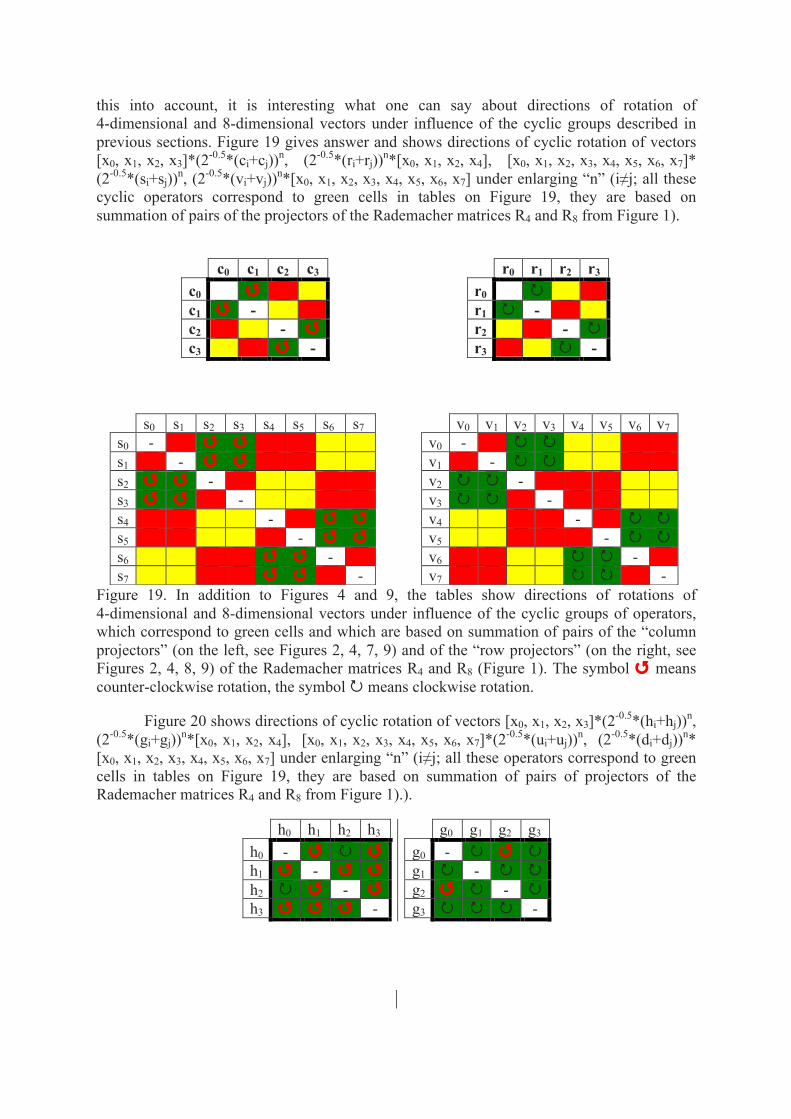
Figure 20 shows directions of cyclic rotation of vectors [x0, x1, x2, x3]*(2-0.5*(hi+hj))n, (2-0.5*(gi+gj))n*[x0, x1, x2, x4], [x0, x1, x2, x3, x4, x5, x6, x7]*(2-0.5*(ui+uj))n, (2-0.5*(di+dj))n* [x0, x1, x2, x3, x4, x5, x6, x7] under enlarging “n” (i≠j; all these operators correspond to green cells in tables on Figure 19, they are based on summation of pairs of projectors of the Rademacher matrices R4 and R8 from Figure 1).).

h0 h1 h2 h3 h0 - Q P Q h1 Q - Q Q h2 P Q - Q h3 Q Q Q -

g0 g1 g2 g3 g0 - P Q P g1 P - P P g2 Q P - P g3 P P P -

u0 u1 u2 u3 u4 u5 u6 u7 u0 - P Q P Q u1 P - Q P Q u2 Q - P Q Q u3 Q P - Q Q u4 P Q - P Q u5 P Q P - Q u6 Q Q Q - P u7 Q Q Q P -

d0 d1 d2 d3 d4 d5 d6 d7 d0 - Q P Q P d1 Q - P Q P d2 P - Q P P d3 P Q - P P d4 Q P - Q P d5 Q P Q - P d6 P P P - Q d7 P P P Q -

Figure 20. In addition to Figures 11 and 16, the tables show directions of rotations of 4-dimensional and 8-dimensional vectors under influence of the cyclic groups of operators, which correspond to green cells and which are based on summation of pairs of the “column projectors” (on the left, see Figures 10, 11, 14, 16) and of the “row projectors” (on the right, see Figures 10, 11, 15, 16) of the Hadamard matrices H4 and H8 (Figure 1). The symbol Q means counter-clockwise rotation, the symbol P means clockwise rotation.

Each of tables on Figures 19 and 20 contains completely different (asymmetrical) number of rotations in the clockwise and counterclockwise. These facts give evidences in favor of an idea that living matter at its basic level of genetic information has certain informational reasons to provide dissymmetry of inherited biological structures and processes. Taking this into account, the author thinks about a possibility of informational reasons for biological dis-symmetry. Here one can remind for a comparison that usually scientists look for reasons of biological dis-symmetry in physical or chemical sciences but not in informatic science.

6. HAMILTON’S QUATERNIONS, COCKLE’S SPLIT-QUATERNIONS, THEIR EXTENSIONS AND PROJECTION OPERATORS

In previous sections we described cases of summation of pairs of the oblique projectors. Now let us consider cases of summation of 4 of these projectors and cases of summation of 8 of these projectors.

The matrix H4 (Figure 1) is sum of the four “column projectors” or the four “row projector” (Figure 10). But H4 has also another decomposition in a form of four sparse matrices H40, H41, H42 and H43 (Figure 21). This set is closed in relation to multiplication and it defines their multiplication table (Figure 21, bottom level) that is identical to the known multiplication table of quaternions by Hamilton. From this point of view, the matrix H4 is the quaternion by Hamilton with unit coordinates. (Such type of decompositions is termed a dyadic-shift decomposition because it corresponds to structures of matrices of dyadic shifts, well known in technology of signals processing [Ahmed, Rao, 1975]).

H4 = H40 + H41 + H42 + H43 = 1 0 0 0 0 1 0 0 0 0 -1 0 0 0 0 1 0 1 0 0 + -1 0 0 0 + 0 0 0 1 + 0 0 1 0 0 0 1 0 0 0 0 1 1 0 0 0 0 -1 0 0 0 0 0 1 0 0 -1 0 0 -1 0 0 -1 0 0 0

1 H41 H42 H43 1 1 H41 H42 H43 H41 H41 - 1 H43 - H42 H42 H42 - H43 - 1 H41 H43 H43 H42 - H41 - 1

Figure 21. The dyadic-shift decomposition of the (4*4)-matrix H4 (from Figure 1) gives the set of 4 sparse matrices H40, H41, H42 and H43, which corresponds to the multiplication table of quatrnions by Hamilton (bottom row). The matrix H40 is identity matrix

Here one can mention that Hamilton quaternions are closely related to the Pauli matrices, the theory of the electromagnetic field (Maxwell wrote his equation on the language of quaternions Hamilton), the special theory of relativity, the theory of spins, quantum theory of chemical valency, etc. In the twentieth century thousands of works were devotes to quaternions in physics [http://arxiv.org/abs/math-ph/0511092]. Now Hamilton quaternions are manifested in the genetic code system. Our scientific direction - "matrix genetics" - has led to the discovery of an important bridge among physics, biology and computer science for their mutual enrichment. In our studies, we have received a new example of the effectiveness of mathematics: abstract mathematical structures, which have been derived by mathematicians at the tip of the pen 160 years ago, are embodied long ago in the information basis of living matter - the system of genetic coding. The mathematical structures, which are discovered by mathematicians in a result of painful reflections (like Hamilton, who has wasted 10 years of continuous thought to reveal his quaternions), are already represented in the genetic coding system.

Let us turn now to the (8*8)-matrix H8 (Figure 1) that can be represented as sum of two matrices HL8 = u0+u2+u4+u6 and HR8 = u1+u3+u5+u7 (Figure 22). Here u0, u1, …, u7 are the «column projectors» from Figure 14.

H8 = HL8+HR8 = 1 0 1 0 -1 0 1 0 0 -1 0 -1 0 1 0 -1 1 0 1 0 -1 0 1 0 0 1 0 1 0 -1 0 1 -1 0 1 0 1 0 1 0 0 1 0 -1 0 -1 0 -1 -1 0 1 0 1 0 1 0 + 0 -1 0 1 0 1 0 1 1 0 -1 0 1 0 1 0 0 -1 0 1 0 -1 0 -1 1 0 -1 0 1 0 1 0 0 1 0 -1 0 1 0 1 -1 0 -1 0 -1 0 1 0 0 1 0 1 0 1 0 -1 -1 0 -1 0 -1 0 1 0 0 -1 0 -1 0 -1 0 1

Figure 22. The representation of the Hadamard matrix H8 (from Figure 1) as sum of two sparse matrices HL8 and HR8

Figure 23 shows a decomposition of the matrix HL8 (from Figure 22) as a sum of 4 matrices: HL8 = HL80 + HL81 + HL82 + HL83. The set of matrices HL80, HL81, HL82 and HL83 is closed in relation to multiplication and it defines the multiplication table that is identical to the multiplication table of quaternions by Hamilton. General expression for quaternions in this case can be written as QL = a0*HL80 + a1*HL81 + a2*HL82 + a3*HL83,

where a0, a1, a2, a3 are real numbers. From this point of view, the (8*8)-genomatrix HL8 is the 4-parametric quaternion by Hamilton with unit coordinates.

HL8 = HL80 + HL81 + HL82 + HL83 =

HL80 HL81 HL82 HL83 HL80 HL80 HL81 HL82 HL83 HL81 HL81 -‐ HL80 HL83 -‐ HL82 HL82 HL82 -‐ HL83 -‐ HL80 HL81 HL83 HL83 HL82 -‐ HL81 -‐ HL80

Figure 23. Upper rows: the decomposition of the matrix HL8 (from Figure 22) as sum of 4 matrices: HL8 = HL80 + HL81 + HL82 + HL83. Bottom row: the multiplication table of these 4 matrices HL80, HL81, HL82 and HL83, which is identical to the multiplication table of quaternions by Hamilton. The matrix HL80 represents the real unit for this matrix set.

The similar situation holds true for the matrix HR8 (from Figure 22). Figure 24 shows a decomposition of the matrix HR8 as a sum of 4 matrices: HR8 = HR80 + HR81 + HR82 + HR83. The set of matrices HR80, HR81, HR82 and HR83 is closed in relation to multiplication and it defines the multiplication table that is identical to the same multiplication table of quaternions by Hamilton. General expression of quaternions in this case can be written as QR = a0*HR80 + a1*HR81 + a2*HR82 + a3*HR83, where a0, a1, a2, a3 are real numbers. From this point of view, the (8*8)-genomatrix HR8 is the quaternion by Hamilton with unit coordinates.

HR8 = HR80 + HR81 + HR82 + HR83 =

1 0 1 0 -1 0 1 0 1 0 1 0 -1 0 1 0 -1 0 1 0 1 0 1 0 -1 0 1 0 1 0 1 0 1 0 -1 0 1 0 1 0 1 0 -1 0 1 0 1 0 -1 0 -1 0 -1 0 1 0 -1 0 -1 0 -1 0 1 0

=

1 0 0 0 0 0 0 0 1 0 0 0 0 0 0 0 0 0 1 0 0 0 0 0 0 0 1 0 0 0 0 0 0 0 0 0 1 0 0 0 0 0 0 0 1 0 0 0 0 0 0 0 0 0 1 0 0 0 0 0 0 0 1 0

+

0 0 1 0 0 0 0 0 0 0 1 0 0 0 0 0 -1 0 0 0 0 0 0 0 -1 0 0 0 0 0 0 0 0 0 0 0 0 0 1 0 0 0 0 0 0 0 1 0 0 0 0 0 -1 0 0 0 0 0 0 0 -1 0 0 0

+

0 0 0 0 -1 0 0 0 0 0 0 0 -1 0 0 0 0 0 0 0 0 0 1 0 0 0 0 0 0 0 1 0 1 0 0 0 0 0 0 0 1 0 0 0 0 0 0 0 0 0 -1 0 0 0 0 0 0 0 -1 0 0 0 0 0

+

0 0 0 0 0 0 1 0 0 0 0 0 0 0 1 0 0 0 0 0 1 0 0 0 0 0 0 0 1 0 0 0 0 0 -1 0 0 0 0 0 0 0 -1 0 0 0 0 0 -1 0 0 0 0 0 0 0 -1 0 0 0 0 0 0 0

0 -1 0 -1 0 1 0 -1 0 1 0 1 0 -1 0 1 0 1 0 -1 0 -1 0 -1 0 -1 0 1 0 1 0 1 0 -1 0 1 0 -1 0 -1 0 1 0 -1 0 1 0 1 0 1 0 1 0 1 0 -1 0 -1 0 -1 0 -1 0 1

= +

0 -1 0 0 0 0 0 0 0 1 0 0 0 0 0 0 0 0 0 -1 0 0 0 0 0 0 0 1 0 0 0 0 0 0 0 0 0 -1 0 0 0 0 0 0 0 1 0 0 0 0 0 0 0 0 0 -1 0 0 0 0 0 0 0 1

+

0 0 0 -1 0 0 0 0 0 0 0 1 0 0 0 0 0 1 0 0 0 0 0 0 0 -1 0 0 0 0 0 0 0 0 0 0 0 0 0 -1 0 0 0 0 0 0 0 1 0 0 0 0 0 1 0 0 0 0 0 0 0 -1 0 0

0 0 0 0 0 1 0 0 0 0 0 0 0 -1 0 0 0 0 0 0 0 0 0 -1 0 0 0 0 0 0 0 1 0 -1 0 0 0 0 0 0 0 1 0 0 0 0 0 0 0 0 0 1 0 0 0 0 0 0 0 -1 0 0 0 0

+

0 0 0 0 0 0 0 -1 0 0 0 0 0 0 0 1 0 0 0 0 0 -1 0 0 0 0 0 0 0 1 0 0 0 0 0 1 0 0 0 0 0 0 0 -1 0 0 0 0 0 1 0 0 0 0 0 0 0 -1 0 0 0 0 0 0

HR80 HR81 HR82 HR83 HR80 HR80 HR81 HR82 HR83 HR81 HR81 -‐ HR80 HR83 -‐ HR82 HR82 HR82 -‐ HR83 -‐ HR80 HR81 HR83 HR83 HR82 -‐ HR81 -‐ HR80

Figure 24. upper rows: the decomposition of the matrix HR8 (from Figure 22) as sum of 4 matrices: H8R = H08R + H18R + H28R + H38R. Bottom row: the multiplication table of these 4 matrices HR80, HR81, HR82 and HR83, which is identical to the multiplication table of quaternions by Hamilton. HR80 represents the real unit for this matrix set

The initial (8*8)-matrix H8 (Figure 1) can be also decomposed in another way on the base of dyadic-shift decomposition. Figure 25 shows such dyadic-shift decomposition H8 = H80+H81+H82+H83+H84+H85+H86+H87, when 8 sparse matrices H80, H81, H82, H83, H84, H85, H86, H87 arise (H80 is identity matrix). The set H80, H81, H82, H83, H84, H85, H86, H87 is closed in relation to multiplication and it defines the multiplication table on Figure 25. This multiplication table is identical to the multiplication table of 8-dimensional hypercomplex numbers that are termed as biquaternions by Hamilton (or Hamiltons’ quaternions over the field of complex numbers). General expression for biquaternions in this case can be written as Q8 = a0*H80+a1*H81+a2*H82+a3*H83+ a4*H84 +a5*H85+a6*H86+a7*H87, where a0, a1, a2, a3, a4, a5, a6, a7 are real numbers. From this point of view, the (8*8)-genomatrix H8 is Hamilton’s biquaternion with unit coordinates.

H8 = H80+H81+H82+H83+H84+H85+H86+H87 = 1 0 0 0 0 0 0 0 0 1 0 0 0 0 0 0 0 0 1 0 0 0 0 0 0 0 0 1 0 0 0 0 0 0 0 0 1 0 0 0 0 0 0 0 0 1 0 0 0 0 0 0 0 0 1 0 0 0 0 0 0 0 0 1

+

0 -1 0 0 0 0 0 0 1 0 0 0 0 0 0 0 0 0 0 -1 0 0 0 0 0 0 1 0 0 0 0 0 0 0 0 0 0 -1 0 0 0 0 0 0 1 0 0 0 0 0 0 0 0 0 0 -1 0 0 0 0 0 0 1 0

+

0 0 1 0 0 0 0 0 0 0 0 1 0 0 0 0 -1 0 0 0 0 0 0 0 0 -1 0 0 0 0 0 0 0 0 0 0 0 0 1 0 0 0 0 0 0 0 0 1 0 0 0 0 -1 0 0 0 0 0 0 0 0 -1 0 0

+

0 0 0 -1 0 0 0 0 0 0 1 0 0 0 0 0 0 1 0 0 0 0 0 0 -1 0 0 0 0 0 0 0 0 0 0 0 0 0 0 -1 0 0 0 0 0 0 1 0 0 0 0 0 0 1 0 0 0 0 0 0 -1 0 0 0

+

0 0 0 0 -1 0 0 0 0 0 0 0 0 -1 0 0 0 0 0 0 0 0 1 0 0 0 0 0 0 0 0 1 1 0 0 0 0 0 0 0 0 1 0 0 0 0 0 0 0 0 -1 0 0 0 0 0 0 0 0 -1 0 0 0 0

+

0 0 0 0 0 1 0 0 0 0 0 0 -1 0 0 0 0 0 0 0 0 0 0 -1 0 0 0 0 0 0 1 0 0 -1 0 0 0 0 0 0 1 0 0 0 0 0 0 0 0 0 0 1 0 0 0 0 0 0 -1 0 0 0 0 0

+

0 0 0 0 0 0 1 0 0 0 0 0 0 0 0 1 0 0 0 0 1 0 0 0 0 0 0 0 0 1 0 0 0 0 -1 0 0 0 0 0 0 0 0 -1 0 0 0 0 -1 0 0 0 0 0 0 0 0 -1 0 0 0 0 0 0

+

0 0 0 0 0 0 0 -1 0 0 0 0 0 0 1 0 0 0 0 0 0 -1 0 0 0 0 0 0 1 0 0 0 0 0 0 1 0 0 0 0 0 0 -1 0 0 0 0 0 0 1 0 0 0 0 0 0 -1 0 0 0 0 0 0 0

1 H81 H82 H83 H84 H85 H86 H87 1 1 H81 H82 H83 H84 H85 H86 H87

H81 H81 -1 H83 - H82 H85 - H84 H87 - H86 H82 H82 H83 -1 - H81 - H86 - H87 H84 H85 H83 H83 - H82 - H81 1 - H87 H86 H85 - H84 H84 H84 H85 H86 H87 -1 - H81 - H82 - H83 H85 H85 - H84 H87 - H86 - H81 1 - H83 H82 H86 H86 H87 - H84 - H85 H82 H83 -1 - H81 H87 H87 - H86 - H85 H84 H83 - H82 - H81 1

Figure 25. Upper rows: the decomposition of the matrix H8 (from Figure 1) as sum of

8 matrices: H8 = H80+H81+H82+H83+H84+H85+H86+H87. Bottom row: the multiplication table of these 8 matrices H80, H81, H82, H83, H84, H85, H86, H87, which is identical to the multiplication table of biquaternions by Hamilton (or Hamiltons’ quaternions over the field of complex numbers). H80 is identity matrix

One can analyze the Rademacher genomatrices R4 and R8 (From Figure 1) by a similar way [Petoukhov, 2012b]). In particular, in this case the following results arise:

• The Rademacher (4*4)-matrix R4 represents split-quaternion by J.Cockle with unit coordinates (http://en.wikipedia.org/wiki/Split-quaternion) in the case of its dyadic-shift decomposition;

• The Rademacher (8*8)-matrix R8 represents bisplit-quaternion by J.Cockle with unit coordinates in the case of its dyadic-shift decomposition;

• If the Rademacher (4*4)-matrix R4 is represented as sum of two sparse matrices (c0+c2) + (c1+c3) (here c0, c1, c2, c3 are the column projectors from Figure 2), then the matrix R4 is sum of two hyperbolic numbers with unit coordunates because each of summands (c0+c2) and (c1+c3) is hyperbolic number with unit coordinates. A similar is true for the case of the “row projectors” r0, r1, r2, r3 from Figure 2.

Now let us pay a special attention to the Rademacher (8*8)-matrix R8 as a sum of the following two sparse matrices RL8 and RR8, the first of which is a sum of 4 projectors with even indexes s0, s2, s4, s6 and the second of which is a sum of 4 projectors with odd indexes s1, s3, s5, s7: R8 = (s0+s2+s4+s6) + (s1+s3+s5+s7) = RL8 + RR8 (here s0, s1, …, s7 are the column projectors from Figure 7). Below this decomposition will be useful for analysis of a correspondence between 64 triplets and 20 amino acids with stop-codons.

R8 = RL8 + RR8 =

1 0 1 0 1 0 -‐1 0 1 0 1 0 1 0 -‐1 0 -‐1 0 1 0 -‐1 0 -‐1 0 -‐1 0 1 0 -‐1 0 -‐1 0 1 0 -‐1 0 1 0 1 0 1 0 -‐1 0 1 0 1 0 -‐1 0 -‐1 0 -‐1 0 1 0 -‐1 0 -‐1 0 -‐1 0 1 0

+

0 1 0 1 0 1 0 -‐1 0 1 0 1 0 1 0 -‐1 0 -‐1 0 1 0 -‐1 0 -‐1 0 -‐1 0 1 0 -‐1 0 -‐1 0 1 0 -‐1 0 1 0 1 0 1 0 -‐1 0 1 0 1 0 -‐1 0 -‐1 0 -‐1 0 1 0 -‐1 0 -‐1 0 -‐1 0 1

Figure 26. The decomposition of the Rademacher (8*8)-genomatrix R8 from Figure 1

Each of these sparse matrices RL8 and RR8 can be decomposed into a set of 4 sparse matrices: RL8= RL80+ RL81+ RL82+RL83 and RR8= RR80+ RR81+ RR82+RR83 (Figures 27 and 28). The first set of matrices RL80, RL81, RL82, RL83 is closed relative to multiplication and it defines a known multiplication table of split-quaternions by J. Cockle (http://en.wikipedia.org/wiki/Split-quaternion) on Figure 27. The second set of matrices RR80, RR81, RR82, RR83 is also closed relative to multiplication and it defines the same multiplication table of split-quaternions by J. Cockle (Figure 28). Consequently, each of matrices RL8 and RR8 is split-quaternion by Cockle with unit coordinates.

RL8= RL80+ RL81+ RL82+RL83 =

1 0 0 0 0 0 0 0 1 0 0 0 0 0 0 0 0 0 1 0 0 0 0 0 0 0 1 0 0 0 0 0 0 0 0 0 1 0 0 0 0 0 0 0 1 0 0 0 0 0 0 0 0 0 1 0 0 0 0 0 0 0 1 0

+

0 0 1 0 0 0 0 0 0 0 1 0 0 0 0 0 -1 0 0 0 0 0 0 0 -1 0 0 0 0 0 0 0 0 0 0 0 0 0 1 0 0 0 0 0 0 0 1 0 0 0 0 0 -1 0 0 0 0 0 0 0 -1 0 0 0

+

+

0 0 0 0 1 0 0 0 0 0 0 0 1 0 0 0 0 0 0 0 0 0 -1 0 0 0 0 0 0 0 -1 0 1 0 0 0 0 0 0 0 1 0 0 0 0 0 0 0 0 0 -1 0 0 0 0 0 0 0 -1 0 0 0 0 0

+

0 0 0 0 0 0 -1 0 0 0 0 0 0 0 -1 0 0 0 0 0 -1 0 0 0 0 0 0 0 -1 0 0 0 0 0 -1 0 0 0 0 0 0 0 -1 0 0 0 0 0 -1 0 0 0 0 0 0 0 -1 0 0 0 0 0 0 0

;

RL80 RL81 RL82 RL83 RL80 RL80 RL81 RL83 RL83 RL81 RL81 - RL80 RL83 - RL82 RL82 RL82 - RL83 RL80 - RL81 RL83 RL83 RL82 RL81 RL80

Figure 27. The decomposition of the matrix RL8 from Figure 26 into the set of 4 matrices RL80, RL81, RL82, RL83, which defines the known multiplication table of split-quaternions by J. Cockle (http://en.wikipedia.org/wiki/Split-quaternion)

RR8= RR80+ RR81+ RR82+RR83 =

0 1 0 0 0 0 0 0 0 1 0 0 0 0 0 0 0 0 0 1 0 0 0 0 0 0 0 1 0 0 0 0 0 0 0 0 0 1 0 0 0 0 0 0 0 1 0 0 0 0 0 0 0 0 0 1 0 0 0 0 0 0 0 1

+

0 0 0 1 0 0 0 0 0 0 0 1 0 0 0 0 0 -1 0 0 0 0 0 0 0 -1 0 0 0 0 0 0 0 0 0 0 0 0 0 1 0 0 0 0 0 0 0 1 0 0 0 0 0 -1 0 0 0 0 0 0 0 -1 0 0

+

+

0 0 0 0 0 1 0 0 0 0 0 0 0 1 0 0 0 0 0 0 0 0 0 -1 0 0 0 0 0 0 0 -1 0 1 0 0 0 0 0 0 0 1 0 0 0 0 0 0 0 0 0 -1 0 0 0 0 0 0 0 -1 0 0 0 0

+

0 0 0 0 0 0 0 -1 0 0 0 0 0 0 0 -1 0 0 0 0 0 -1 0 0 0 0 0 0 0 -1 0 0 0 0 0 -1 0 0 0 0 0 0 0 -1 0 0 0 0 0 -1 0 0 0 0 0 0 0 -1 0 0 0 0 0 0

;

RR80 RR81 RR82 RR83 RR80 RR80 RR81 RR83 RR83 RR81 RR81 - RR80 RR83 - RR82 RR82 RR82 - RR83 RR80 - RR81 RR83 RR83 RR82 RR81 RR80

Figure 28. The decomposition of the matrix RR8 from Figure 26 into the set of 4 matrices RR80, RR81, RR82, RR83, which defines the same multiplication table of split-quaternions by J. Cockle (http://en.wikipedia.org/wiki/Split-quaternion)

But each of the same (8*8)-matrices RL8 and RR8 (Figure 26)) can be decomposed in another way, which leads to its representation in a form of sum of two hyperbolic numbers: RL8= (s0+s4)+(s2+s6) and RR8=(s1+s5)+(s3+s7), where is s0, s1, …, s7 are column projectors from the decomposition of R8 on Figure 7. Figure 29 shows that each of sums (s0+s4), (s2+s6), (s1+s5), (s3+s7) in these decompositions for RL8 and RR8 is a (8*8)-matrix representation of hyperbolic number, whose coordinates are equal to 1. It means also that the whole (8*8)-matrix R8 is sum of 4 hyperbolic numbers, whose coordinates are equal to 1, in an 8-dimensional space. These decompositions are useful for analyzing the degeneration of the genetic code in next Sections.

s0+s4 =

1 0 0 0 1 0 0 0 1 0 0 0 1 0 0 0 -1 0 0 0 -1 0 0 0 -1 0 0 0 -1 0 0 0 1 0 0 0 1 0 0 0 1 0 0 0 1 0 0 0 -1 0 0 0 -1 0 0 0 -1 0 0 0 -1 0 0 0

=

1 0 0 0 0 0 0 0 1 0 0 0 0 0 0 0 -1 0 0 0 0 0 0 0 -1 0 0 0 0 0 0 0 0 0 0 0 1 0 0 0 0 0 0 0 1 0 0 0 0 0 0 0 -1 0 0 0 0 0 0 0 -1 0 0 0

+

0 0 0 0 1 0 0 0 0 0 0 0 1 0 0 0 0 0 0 0 -1 0 0 0 0 0 0 0 -1 0 0 0 1 0 0 0 0 0 0 0 1 0 0 0 0 0 0 0 -1 0 0 0 0 0 0 0 -1 0 0 0 0 0 0 0

= e0+e4;

e0 e4

e0 e0 e4

e4 e4 e0

s2+s6 =

0 0 1 0 0 0 -1 0 0 0 1 0 0 0 -1 0 0 0 1 0 0 0 -1 0 0 0 1 0 0 0 -1 0 0 0 -1 0 0 0 1 0 0 0 -1 0 0 0 1 0 0 0 -1 0 0 0 1 0 0 0 -1 0 0 0 1 0

=

0 0 1 0 0 0 0 0 0 0 1 0 0 0 0 0 0 0 1 0 0 0 0 0 0 0 1 0 0 0 0 0 0 0 0 0 0 0 1 0 0 0 0 0 0 0 1 0 0 0 0 0 0 0 1 0 0 0 0 0 0 0 1 0

+

0 0 0 0 0 0 -1 0 0 0 0 0 0 0 -1 0 0 0 0 0 0 0 -1 0 0 0 0 0 0 0 -1 0 0 0 -1 0 0 0 0 0 0 0 -1 0 0 0 0 0 0 0 -1 0 0 0 0 0 0 0 -1 0 0 0 0 0

= e2+e6;

e2 e6

e2 e2 e6

e6 e6 e2

s1+s5 =

0 1 0 0 0 1 0 0 0 1 0 0 0 1 0 0 0 -1 0 0 0 -1 0 0 0 -1 0 0 0 -1 0 0 0 1 0 0 0 1 0 0 0 1 0 0 0 1 0 0 0 -1 0 0 0 -1 0 0 0 -1 0 0 0 -1 0 0

=

0 1 0 0 0 0 0 0 0 1 0 0 0 0 0 0 0 -1 0 0 0 0 0 0 0 -1 0 0 0 0 0 0 0 0 0 0 0 1 0 0 0 0 0 0 0 1 0 0 0 0 0 0 0 -1 0 0 0 0 0 0 0 -1 0 0

+

0 0 0 0 0 1 0 0 0 0 0 0 0 1 0 0 0 0 0 0 0 -1 0 0 0 0 0 0 0 -1 0 0 0 1 0 0 0 0 0 0 0 1 0 0 0 0 0 0 0 -1 0 0 0 0 0 0 0 -1 0 0 0 0 0 0

= e1+e5;

e1 e5

e1 e1 e5

e5 e5 e1

s3+s7 =

0 0 0 1 0 0 0 -1 0 0 0 1 0 0 0 -1 0 0 0 1 0 0 0 -1 0 0 0 1 0 0 0 -1 0 0 0 -1 0 0 0 1 0 0 0 -1 0 0 0 1 0 0 0 -1 0 0 0 1 0 0 0 -1 0 0 0 1

=

0 0 0 1 0 0 0 0 0 0 0 1 0 0 0 0 0 0 0 1 0 0 0 0 0 0 0 1 0 0 0 0 0 0 0 0 0 0 0 1 0 0 0 0 0 0 0 1 0 0 0 0 0 0 0 1 0 0 0 0 0 0 0 1

+

0 0 0 0 0 0 0 -1 0 0 0 0 0 0 0 -1 0 0 0 0 0 0 0 -1 0 0 0 0 0 0 0 -1 0 0 0 -1 0 0 0 0 0 0 0 -1 0 0 0 0 0 0 0 -1 0 0 0 0 0 0 0 -1 0 0 0 0

= e3+e7;

e3 e7

e3 e3 e7

e7 e7 e3

Figure 29. Decompositions of sums of projectors (s0+s4), (s2+s6), (s1+s5), (s3+s7), which show that each of these sums is an (8*8)-matrix representation of hyperbolic numbers, whose coordinates are equal to 1, in an 8-dimensional space.

7. GENETIC MATRICES AS SUMS OF TENSOR PRODUCTS OF OBLIQUE (2*2)-PROJECTORS. EXTENSIONS OF GENETIC MATRICES INTO (2N*2N)-MATRICES

The Rademacher matrices R4 and R8 and also Hadamard matrices H4 and H8 (Figure 1) are interconnected by means of the following expressions:

R4 U [1 1; 1 1] = R8, H4 U [1 -1; 1 1] = H8 (1)

where U means tensor multiplication; the matrix [1 1; 1 1] is a traditional (2*2)-matrix representation of hyperbolic number with unit coordinates; the matrix [1 -1; 1 1] is a traditional (2*2)-matrix representation of complex number with unit coordinates.

The following extensions of the expressions (1) lead to (2n*2n)-matrices RK and HK (where K=2n, n = 4, 5, 6,…; (n-2) means a tensor power):

R4 U [1 1; 1 1](n-2) = RK, H4 U [1 -1; 1 1](n-2) = HK (2)

In this algorithmic way we get a great set of (2n*2n)-matrices RK and HK, each of which can be represented as a sum of 2n «column projectors» (or 2n «row projectors») by analogy with cases described above. Summations of these new «column projectors» (and also «row projectors») in different combinations (in pairs, in fours, in eights, etc.) give many new operators, exponentiation of which generates a great number of cyclic groups and other kind of operators. They also give many new representations of complex numbers, hyperbolic numbers, Hamilton’s quaternion, split-quaternions and their extensions in a form of (2n*2n)-matrices that correspond to 2n-dimensional spaces. These new operators possess many similar properties, including a selective control (or coding) of different subspaces in 2n-dimensional space, in analogy with operators described in previous sections.

Why one can declare that each of matrices in the «column decomposition» (or in the «row decomposition») of any of matrices Rk and Hk in the expressions (2) is a projection operator? It can be declared on basis of the following simple theorem, taking into account that main diagonals of all matrices Rk and Hk contains only entries +1.

Theorem: any sparse square matrix P, which contains only a single non-zero column or a single non-zero row and which has its entry +1 on the main diagonal, is a projection operator (it satisfies the criterion P2=P).

Proof. When multiplying two matrices |Aik| and |Bkj|, the elements of the rows in the first matrix are multiplied with corresponding columns in the second matrix to receive the resulting matrix (AB)ij| = A!

!!! ik*Bkj (http://en.wikipedia.org/wiki/Matrix_multiplication ). Let us consider a case of a square matrix |Pij| (here i,j = 1, 2,…, m) with only a single non-zero column Pis ≠ 0, which is numerated by an index “s” and which contains +1 in its cell on the main diagonal of this matrix: Pss = 1. It means that all entries Pik = 0 if k≠s. The second degree of this matrix gives a square matrix:

P!

!!! ik*Pkj = P!!!! ik*Pks (3)

But among all Pik only one column differs from zero: Pis≠0. In the equation (3), Pis corresponds to the second factor Pss = 1. By these reasons we have Pis*Pss = Pis for the equation (3). So the sparse square matrix |Pij|2 contains only the same single non-zero column Pis like as the matrix |Pij|. Consequently |Pij|2=|Pij|; in other words, this matrix |Pij| is a projection operator, Q.E.D. The case of similar representations of such 2n*2n-matrices on basis of a sum of “row projectors” has its proof by analogy.

This theorem allows making the following conclusion about any variant of matrix presentations of complex numbers, hyperbolic numbers and their extensions into 2n-dimensional numerical systems (including Hamilton's quaternions and biquaternions, split-quaternions and bisplit-quaternions by Cockle, etc.): if the real part of such 2n-dimensional number is equal to +1, then its matrix presentation is a sum of 2n «column projectors» (and «row projectors»). It is provided by the fact that real parts of such multidimensional numerical systems are represented by matrix diagonal that contains only entries +1. Figure 30 shows an example of one of matrix presentations of Hamilton quaternions in a case when their real parts are equal to +1.

1 b c d 1 0 0 0 0 b 0 0 0 0 c 0 0 0 0 d -b 1 -d c = -b 0 0 0 + 0 1 0 0 + 0 0 -d 0 + 0 0 0 c -c d 1 -b -c 0 0 0 0 d 0 0 0 0 1 0 0 0 0 -b -d -c b 1 -d 0 0 0 0 -c 0 0 0 0 b 0 0 0 0 1

Figure 30. The "column decomposition" of the classical (4*4)-matrix representation of Hamilton's quaternions (http://en.wikipedia.org/wiki/Quaternion#Matrix_representations) in cases when their real parts are equal to +1. Each of 4 matrices (on the right) is a projection operator in accordance with the described theorem. Here b, c, d are real numbers.

So, many kinds of hypercomplex numbers are based on sums of projectors. In this sense the notion "projectors" can be considered as more fundemental than the notion "hypercomplex numbers" of the mentioned types. Many of these hypercomplex numbers are applied widely in different fields of science: physics, chemistry, informatics, etc. Awareness of the fact that these systems of hypercomplex numbers are based on sums of projectors may help in a rethinking of existing theories and in developing new theories in the field of mathematical natural science. In particularly, it concerns Hamilton's quaternions. For example, Maxwell has used them in creation of his equations of electro-magnetic field. Could one develop an alternative description and development of the theory of electro-magnetic field on basis of sums of appropriate projectors? It is one of many open questions in theoretical aplications of projectors.

Now we show that each of genetic Rademacher and Hadamard matrices (including R2, R8, H4, H8 from Figure 1 and their extensions into 2n*2n-matrices RK and HK in expressions (2)) can be expressed as sums and tensor multiplications of four (2*2)-matrices of «column projectors» (or of analogical «row projectors»). Figure 31 shows these 4 basic (2*2)-projectors, which are marked by 4 different colours for visibility, and some examples of expressions of a few Rademacher and Hadamard matrices by means of their using.

1 0 1 0

;

1 0 -1 0

;

0 -1 0 1

;

0 1 0 1

1 1 1 1

=

1 0 1 0

+

0 1 0 1

;

1 -1 1 1

=

1 0 1 0

+

0 -1 0 1

R4= 1 0 1 0

V

1 0 -1 0

+

0 1 0 1

V

1 0 -1 0

+

1 0 -1 0

V

0 1 0 1

+

0 -1 0 1

V

0 1 0 1

H4= 1 0 1 0

V

1 0 -1 0

+

0 -1 0 1

V

1 0 -1 0

+

1 0 -1 0

V

0 1 0 1

+

0 1 0 1

V

0 1 0 1

Figure 31. Examples of using the 4 basic (2*2)-projectors (upper level) to express (2*2)-matrix representations of hyperbolic number and of complex number with unit coordinates (the second level) and to express the Rademacher (4*4)-matrix R4 and the Hadamard (4*4)-matrix H4 from Figure 1 (two lower levels)

One can also note that every of the genetic “column (2n*2n)-projectors” and the “row (2n*2n)-projectors” can be expressed by means of tensor multiplications of appropriate (2*2)-projectors from their basic set of the 4 projectors (Figure 31, upper level). It means that cases of 2-dimensional spaces can be considered as basic in this model approach. It is interesting because of the known fact that namely 2-dimensional sub-spaces play a fundamental role in morphological organization and development of living bodies (see for example about a fundamental role of primary tissue layers or primary germ layers in http://en.wikipedia.org/wiki/Germ_layer; in accordance with germ layer theory, for example, all different organs of human bodies develop from one of the 3 germ layers).

8. AN APPLICATION OF OBLIQUE PROJECTORS TO SIMULATE ENSEMBLES OF PHYLLOTAXIS PATTERNS IN LIVING BODIES

In the field of mathematical biology, phyllotaxis phenomena are one of the most known [Adler, Barabe, Jean, 1997; Jean, 1995; http://www.goldenmuseum.com/0604Phillotaxis_engl.html]. Usually phyllotaxis laws are described as those inherited spiral-like dislocations of leaves and some other parts of plants, which are connected with Fibonacci numbers. But the similar phyllotaxis laws dictate also inherited configurations of some biological molecules, parts of animal bodies, etc. (see, for example, a review in [Jean, 1995]). In other words, phyllotaxis laws appear in inherited morphological structures at very different levels and branches of biological evolution. Figure 32 shows a few examples of phyllotaxis spirals.

1

2

3

4

5

6

Figure 32. Examples of phyllotaxis patterns: 1) sunflower; 2) alloe (from http://radiolus.com/index.php/nepoznannoe/255-paradoksy-posledovatelnosti-chisel-fibonachchi ); 3) a pine cone (from http://www.maths.surrey.ac.uk/hosted-sites/R.Knott/Fibonacci/fibnat.html); 4) a seashell (from http://www.eb.tuebingen.mpg.de/?id=476 ); 5) a fractal vegetable Romanesco Broccoli (Brassica oleracea) (from http://egregores.blogspot.ru/2010/12/extremely-cool-natural-fractals.html ); 6) a spruce with cones (from http://foto.rambler.ru/users/nadezhda-rodnaja/albums/53780408/photo/4e9c302c-1a1a-3e9d-c61e-db70c258d714/ )

On Figure 32, images 5 and 6 illustrate that a whole organism can contain many parts with similar phyllotaxis patterns in each (like as a spruce with many phyllotaxis cones). For physicist or mathematician is natural to think that such organism can be modelled as a multidimensional phase space (or a configuration space) with an appropriate number of similar subspaces, each of which receives the same phyllotaxis pattern due to a selective control of subspaces or their selective genetic coding. Such selective control or coding in this phase space should be based on an appropriate system of operators (about a phase space see http://en.wikipedia.org/wiki/Phase_space).

Our model approach allows such modelling due to a discovered system of operators based on described sums of oblique projectors (including 2n*2n-dimensional matrices Rk and Hk in expressions (2)), which have such properties of a selective control (or coding) of subspaces of 2n-dimensional space. In other words, we propose an approach to model ensembles of phyllotaxis patterns (or other patterns and processes) inside a multidmensional phase space that represents a whole organism. The described system of operators for a

selective control or coding can be conditionally named briefly as a «genetic system of operators» (or more briefly, «G-system of operators). As we can judge, in the field of phyllotaxis study, other authors didn’t simulate such ensembles of phyllotaxis patterns though many different models of separate patterns (without their ensembles in a joint phase space) exist. In addition, known models of inherited phyllotaxis patterns don’t associate them with structural properties of the genetic coding system in contrast to our genetic approach. Let us explain our model approach to phyllotaxis phenomena in more details.

It is known that classical phyllotaxis patterns arise in the result of iterative rotations of initial object approximately on an angle 1370 with a simultaneous increase of its distance from the center of the phyllotaxis pattern. On a complex plane such iterative operations can be simulated by means of iterative multiplication of an initial vector (or a point) with appropriate complex number z = x+i*y, which provides such angle of rotation (due to its appropriate argument) and increase (due to its appropriate modulus) in accordance with known properties of complex numbers. The described G-system of operators, which contains many variants of sparse 2n*2n-matrix presentations of complex numbers on basis of sums of some genetic projectors (from "column decompositions" of 2n*2n-matrices RK and HK in expressions (2)), allows generating many phyllotaxis patterns, each of which belong to its own 2-dimensional plane inside a whole phase space. In these cases, each of phyllotaxis patterns in a separate phase plane can have its own degree of maturation (or development) and its own type of a phyllotaxis picture; it depends on a kind of complex numbers, which is chosen for its iterative generating.

This model approach does not pretend to a new explanation for existence of Fibonacci numbers in phyllotaxis patterns. But this model approach give abilities to simulate bunches of phyllotaxis patterns in separate organisms. Concerning to Fibonacci or Luca numbers in phyllotaxis laws, one should remind here that “the phyllotaxis rules … cannot be taken as applying to all circumstances, like a law of nature. Rather, in the words of the famous Canadian mathematician Coxeter, they are 'only a fascinatingly prevalent tendency" (http://goldenratiomyth.weebly.com/phyllotaxis-the-fibonacci-sequence-in-nature.html ). One can think that the role of iterative operations in living nature is much more important than particular realizations of Fibonacci or Luca numbers.

To simulate an ensemble of phyllotaxis 3d-patterns (an ensemble of many cones of a spruce, etc.), each of which belongs to a separate subspace of a whole 2n*2n-dimensional phase space, an iterative application of Hamilton's quaternions can be used in their 2n*2n-matrix forms of presentation in the described G-system of operators.

In addition the author reminds here about cyclic groups on basis of Hamilton’s quaternion and biquaternion with unit coordinates: these cyclic groups allow simulating some heritable biological phenomena including color perception, properties of which correspond to the Newton’s color circle (see [Petoukhov, 2011b] and Section 17 in [Petoukhov, 2012a]). Using Hamilton’s quaternions and biquaternions as 2n*2n-operators from the described G-system allows simulating some inherited ensembles of biological patterns including some inherited ensembles of color patterns and color changes of biological bodies.

9. HYPERBOLIC NUMBERS, GENETIC PROJECTORS AND THE WEBER-FECHNER LAW OF PSYCHOPHYSICS

This Section is devoted to hyperbolic numbers in separate planes of 2N-dimensional spaces, their connections with some genetic projectors (from Figures 2, 4-6, 8 and 9) and

with inherited psychophysical phenomena. The name «hyperbolic» for this kind of 2-dimensional numbers is traditionally used because of their connection with hyperbolas and hyperbolic rotations (http://en.wikipedia.org/wiki/Split-complex_number, http://www.physicsinsights.org/hyperbolic_rotations.html ). Hyperbolic numbers have properties corresponding to Lorentz group of two-dimensional Special Relativity (www.springer.com/.../9783642179761-c1.pdf?, , http://garretstar.com/secciones/publications/docs/HYP2.PDF ).

Gxy = x*1+y*i =

x, y y, x

= x*

1 0 0 1

+ y*

0 1 1 0

;

1 i 1 1 i i i 1

J = x*1+(x2-‐a)0.5*i =

x, (x2-‐a)0.5 (x2-‐a)0.5, x

= x*

1 0 0 1

+ (x2-‐a)0.5*

0 1 1 0

Figure 33. Upper level: the matrix representation of hyperbolic numbers, where two sparse (2*2)-matrices represent real and imaginary units (1 and i) of these numbers. The multiplication table of these basic elements 1 and i is shown on the right side. Bottom level: the special case of the set of hyperbolic numbers J (with the fixed value “a”) describes a hyperbola x2+y2=a, where “x” is a variable.

Hyperbolic numbers Gxy = x*1+y*i (where «i» is the imaginary unit of hyperbolic numbers with its property i2=+1) have a known (2*2)-matrix form of their representation shown on Figure 33. A special case of hyperbolic numbers

J=[x, (x2-a)0.5; (x2-a)0.5, x] (4)

(where “x” is a variable and the parameter “a” is fixed) describes a hyperbola, which corresponds to the equation x2+y2=a. This equation describes the hyperbola in the coordinate system (x,y), axes of which coincide with axes of symmetry of the hyperbole. In another coordinate system, axes of which coincide with asymptotes of the hyperbola, the same hyperbola is described by the equation y=a/x (Figure 34). Any point of any hyperbola can be transformed into a new point of the same hyperbola by means of so called hyperbolic rotation, which is described by the same matrix representation of hyperbolic numbers [x, y; y, x] if its determinant is equal to 1.

It is known that hyperbolic numbers and hyperbolic operators are closely connected with natural logarithms, which can be defined on the base of hyperbolic rotations because of their relations with values of area under hyperbolas (http://mathworld.wolfram.com/NaturalLogarithm.html). By this reason natural logarithm «was formerly called hyperbolic logarithm as it corresponds to the area under a hyperbola» (http://en.wikipedia.org/wiki/Natural_logarithm ). Area s of a curvilinear trapezoid inside boundaries, which are created by the hyperbola x*y = a, the x-axis and the lines x = x0 and x = x1, is equal to

s = a*ln(x1/x0) = a*{ln(x1)-ln(x0)}, (5)

where ln – natural (or hyperbolic) logarithm (Figure 34). History of hyperbolic logarithms is described for example in the book [Klein, 2009].

Figure 34. The function a*ln(x1/x0) is illustrated as the area under the hyperbola y = a/x from x0 to x1.

But a wide class of genetically inherited physiological phenomena is organized by the nature by means of the same logarithmic law (5) and it can be described mathematically on the base of hyperbolic numbers. We mean here the main psychophysiologic law by Weber-Fechner (http://en.wikipedia.org/wiki/Weber–Fechner_law): the intensity of the perception is proportional to the logarithm of stimulus intensity; it is expressed by the equation

p = k*ln(V/V0) = k*{ln(V) - ln(V0)}, (6)

where p - the intensity of perception, V - stimulus, V0 - threshold stimulus, ln - natural logarithm. Proportionality factor k in the expression (6) is different for different channels of sensory perception (vision, hearing, etc.); this difference of values «k» is associated with different values "a" in the equation of the hyperbola: x*y = a. The threshold stimulus V0 in (5) is also different for different channels of sensory perception.

The identity of expressions (5) and (6) allows to propose a geometric model of the Weber-Fechner law on the base of the described matrix representation of hyperbolic numbers in connection with a phenomenology of the molecular-genetic system. In this model the threshold stimulus V0 in the expression (6) is interpreted as the value x0 from the expression (5); the proportionality factor “k” in (6) is interpreted as the value “a” from (5); the stimulus V(t), which is varied in time, is interpreted as the variable x(t) from (5) and the perception “p" in (6) is interpreted as the area “s” from (5). Taking into account the type of hyperbolic numbers J from the expression (4), it is obvious that the hyperbolic number J0=[x0, (x0

2-a)0.5; (x0

2-a)0.5, x0] corresponds to the fixed area s0=a*ln(x0) of the curvilinear trapezoid, points of which have their x-coordinates inside the interval from 1 till x0; another hyperbolic number J=[x, (x2-a)0.5; (x2-a)0.5, x0] corresponds to the area sx=a*ln(x) of the curvilinear trapezoid with its x-coordinates inside the bigger interval from 1 till x. The total area s of the third curvilinear trapezoid, points of which have their x-coordinates inside the interval from x0 till x, is equal to difference sx-s0, that is

s = sx-s0 = a*ln(x) - a*ln(x0) = a*ln(x1/x0) (7)

This curvilinear trapezoid with its area s corresponds to the hyperbolic number, which is equal to the following:

J - J0 = [(x-x0), ((x-x0)2-a)0.5; ((x-x0)2-a)0.5, x0] (8)

We have described the geometric model for the case of one sensory channel. Let us

generalize now this geometric model for a case of a multi-dimensional space with different 2-dimensional planes inside it, each of which contains the described hyperbolic model of the Weber-Fechner law for one of many sensory channels of an organism. It is known that different types of inherited sensory perception are subordinated to this law: sight, hearing, smell, touch, taste, etc. One can suppose that the Weber–Fechner law is the law specially for nervous system. But it is not true since its meaning is much more wider because it is realized in many kinds of lower organisms without a nervous system in them: “this law is applicable to chemo-tropical, helio-tropical and geo-tropical movements of bacteria, fungi and antherozoids of ferns, mosses and phanerogams .... The Weber-Fechner law, therefore, is not the law of the nervous system and its centers, but the law of protoplasm in general and its ability to respond to stimuli" [Shultz, 1916, p. 126]. So the whole system of perception of an organism demonstrates itself as a multi-parametric system with many sub-systems of perception, which are subordinated to the logarithmic Weber-Fechner law. A generalized model of multi-dimensional space with appropriate sub-spaces is needed to describe this inherited multi-channel organization of the logarithmic perception in the case of the whole living organism. Let us show that our approach on the base of sums of genetic projectors allows to create such generalized model.

Hyperbolic numbers Gxy=x*1+y*i have the multiplication table of their real and imaginary units shown on Figure 33. But the same multiplication table of hyperbolic numbers we have already received above:

• on Figures 5 and 6 for sums (c0+c2), (c1+c3), (r0+r3), (r1+r2) of genetic (4*4)-projectors c0, c1, c2, c3, r0, r1, r2, r3 from Figure 2;

• on Figure 29 for sums (s0+s4), (s1+s5), (s2+s6), (s3+s7) of genetic (8*8)-projectors s0, s1,…, s7 from Figure 7.

It means that these sums of genetic (4*4)- and (8*8)-projectors are matrix representations of hyperbolic numbers with unit coordinates in corresponding 2-dimensional planes of 4-dimensional and 8-dimensional spaces. On the basis of each of these sums, one can construct a general representation of hyperbolic numbers (with an arbitrary values of their coordinates) in an appropriate hyperbolic plane of such multi-dimensional space. For example, if e0 and e4 are (8*8)-matrices taken from the decomposition of the (8*8)-matrix s0+s4 on Figure 29, then the expression G04=a0*e0+b4*e4 represents the hyperbolic number with real coordinates «a0» and «b4» in the plane (x0, x4) inside an 8-dimensional space with its coordinate system (x0, x1, …, x7). Similar situations holds true for expressions G15=a1*e1+b5*e5, G26=a2*e2+b6*e6, G37=a3*e3+b7*e7, each of which represents hyperbolic number in an appropriate plane inside (8*8)-dimensional space, if e1, e2, e3, e5, e6, e7 are (8*8)-matrices taken from decompositions on Figure 29. The (8*8)-matrix G04+G15+G26+G37 represents an operator of an 8-dimensional space with a set of 4 hyperbolic planes (x0, x4), (x1, x5), (x2, x6), (x3, x7) inside it.

For each of these four 2-dimensional planes (x0, x4), (x1, x5), (x2, x6), (x3, x7) of an 8-dimensional space one can choose an individual hyperbola x2-y2=a and an individual threshold stimulus x0 to create the hyperbolic model of the Weber-Fechner law in the united set of four perception channels of the organism. In this case we have the following expression of the model for each of the planes, if we take (8*8)-matrices e0, e1, …, e7 from Figure 29 to express real and imaginary units of hyperbolic numbers (here V0, V1, V2, V3 mean stimulus variables on x0-, x1-, x2-, x3-axis correspondingly; V00, V01, V02, V03 mean threshold stimuluses on the same x0-, x1-, x2-, x3-axis correspondingly; parameters a0, a1, a2, a3 for

corresponding planes mean the parameter “a” from the general equation x2-y2=a of hyperbola; S04, S15, S26, S37 mean area of corresponding trapezoids defined by the hyperbolic numbers in these four planes; parameters k0, k1, k2, k3 for corresponding planes mean the parameter k from (6)):

• for the plane (x0, x4): G04=(V0-V00)*e0+{(V0-V00)2-a0)0.5}*e4; this hyperbolic number G04 corresponds to the area S04= k0*ln(V0/V00), which simulates the Weber-Fechner law in the plane (x0, x4);



• for the plane (x3, x7): G37=(V3-V03)*e3+{(V3-V03)2-a0)0.5}*e7; this hyperbolic number G37 corresponds to the area S37= k3*ln(V3/V03), which simulates the Weber-Fechner law in the plane (x3, x7).

Figure 35 shows the (8*8)-matrix W, which represents the sum of the (8*8)-matrix representations of these hyperbolic numbers: W=G04+G15+G26+G37. One can see that the (8*8)-matrix W on Figure 35 has a special structure: its both (4*4)-quadrants along each diagonals are identical to each other. This fact allows expressing the matrix W in the following form:

W = [1 0; 0 1]VM0 + [0 1; 1 0]VM1 , (9)

where [1 0; 0 1] and [0 1; 1 0] are matrix representations of real and imaginary units of hyperbolic numbers; M0 is the (4*4)-matrix, which reproduces each of (4*4)-quadrants along the main diagonal; M1 is the (4*4)-matrix, which reproduces each of (4*4)-quadrants along the second diagonal. The expression (9) means that the matrix W belongs to so called «tensornumbers» (more precisely, to a category of «tensorhyperbolic numbers»), which will be introduced below in a special Section.

Our approach, which was described above on the base of genetic matrices, allows natural modeling such kind of 2N-parametric systems with its 2-parametric hyperbolic sub-systems by means of the described type of a (2N*2N)-matrix operator of a 2N-dimensional space with appropriate quantity of hyperbolic planes inside it (in this case each of hyperbolic planes corresponds to an individual channel of perception with its own coefficient k and the threshold value V0 in the expression (6)). This (2N*2N)-matrix operator also belongs to the category of tensorhyperbolic numbers, because it can be expressed by means of the expression (9), where M0 and M1 are (2N-1*2N-1)-matrices.

(V0-V00) (V1-V01) (V2-V02) (V3-V03) {(V0-V00)2-a0)0.5}

{(V1-V01)2-a1)0.5}

-{(V2-V02)2-a2)0.5}

-{(V3-V03)2-a0)0.5}

(V0-V00) (V1-V01) (V2-V02) (V3-V03) {(V0-V00)2-a0)0.5}

{(V1-V01)2-a1)0.5}

-{(V2-V02)2-a2)0.5}

-{(V3-V03)2-a0)0.5}

-(V0-V00) -(V1-V01) (V2-V02) (V3-V03) -{(V0-V00)2-a0)0.5}

-{(V1-V01)2-a1)0.5}

-{(V2-V02)2-a2)0.5}

-{(V3-V03)2-a0)0.5}

-(V0-V00) -(V1-V01) (V2-V02) (V3-V03) -{(V0-V00)2-a0)0.5}

-{(V1-V01)2-a1)0.5}

-{(V2-V02)2-a2)0.5}

-{(V3-V03)2-a0)0.5}

{(V0-V00)2-a0)0.5}

{(V1-V01)2-a1)0.5}

-{(V2-V02)2-a2)0.5}

-{(V3-V03)2-a0)0.5}

(V0-V00) (V1-V01) (V2-V02) (V3-V03)

{(V0-V00)2-a0)0.5}

{(V1-V01)2-a1)0.5}

-{(V2-V02)2-a2)0.5}

-{(V3-V03)2-a0)0.5}

(V0-V00) (V1-V01) (V2-V02) (V3-V03)

-{(V0-V00)2-a0)0.5}

-{(V1-V01)2-a1)0.5}

-{(V2-V02)2-a2)0.5}

-{(V3-V03)2-a0)0.5}

-(V0-V00) -(V1-V01) (V2-V02) (V3-V03)

-{(V0-V00)2-a0)0.5}

-{(V1-V01)2-a1)0.5}

-{(V2-V02)2-a2)0.5}

-{(V3-V03)2-a0)0.5}

-(V0-V00) -(V1-V01) (V2-V02) (V3-V03)

Figure 35. The matrix representation of the sum W=G04+G15+G26+G37 of the hyperbolic numbers G04, G15, G26, G37, which belong to four planes (x0, x4), (x1, x5), (x2, x6), (x3, x7) inside the 8-dimensional space (explanation in the text).

So we have two important facts:

• the logarithmic Weber-Fechner law has a total meaning for different sub-systems of perception inside the whole perception system of organism;

• this unity of all subsystems of perception inside the whole organism, which are subordinated to the Weber-Fechner law, can be expressed by means of 2N-dimensional tensorhyperbolic numbers by analogy with the expression (9).

These facts allow the author to put forward the following statement (or hypothesis): a living organism percepts an external world as a multi-parametric system, which belongs to a tensorhyperbolic category. In other words, for the whole perception system of a living organism, the external world is a life of tensorhyperbolic numbers in time. Correspondingly, interrelations of a living organism with the external world are realized on the base of processing of percepted tensorhyperbolic numbers, which are systematically changed over time in accordance with changes of external stimuluses (in addition, the author believes that a living organism can be regarded as a life of tensornumbers over time; in this approach tensorcomplex numbers and their extensions deserve special attention). This mathematical approach to phenomenology of perception of the world is closely connected with the multi-parametric system of the genetic coding in its matrix form of representation; such connection allows a genetical transfer of this general biological property along a chain of generations.

10. REFLECTION OPERATORS AND GENETIC PROJECTORS.

By definition, a linear operator L is the reflection operator (or briefly, a "reflection") if and only if it satisfies the following criterion: L2 = E, where E is the identity operator (it is also denoted as «1»), that is the real unit (see for example [Vinberg, 2003, Chapter 6]). The

imaginary unit «i» of hyperbolic numbers satisfies this criterion and consequently it is the reflection operator: i2=+1 (see Figure 33). Hyperbolic number with unit coordinates (1+i) is sum of the identity operator «1» and the reflection operator «i». The well-known (2*2)-matrix represenation of the imaginary unit is the following: [0 1; 1 0] (Figure 33). The acion of this reflection operator on a voluntary 2-dimensional vector generates a new vector, which is a mirror-symmetrical analogue of the initial vector relative to the bisector of the angle between the x-axis and y-axis of the coordinate system (x, y). For example, [3, 5]*[0 1; 1 0] = [5, 3]. A reflection is an involution: when applied twice in succession, every point returns to its original location, and every geometrical object is restored to its original state.

But we have shown above that many of sums of genetic projectors are the (2N*2N)-matrix representation of hyperbolic numbers, which have their own real and imaginary units in respective planes inside 2N-dimensional space (see for example Figures 5, 6 and 29). Correspondingly, imaginary units of these hyperbolic numbers are (2N*2N)-operators of reflections in these planes inside 2N-dimensional space. It gives evidences in favor of that the system of genetic coding actively uses also reflection operators. It is interesting because mirror reflections exist in many genetically inherited biological structures, including left and right halves of human and animal bodies. In the author's laboratory, the genetic (2N*2N)-matrices of reflection operators are used to analyze mirror symmetries in molecular-genetic systems including long genetic sequences, genetic palindromes, chromosomal inversion, etc.

11. THE SYMBOLIC MATRICES OF GENETIC DUPLETS AND TRIPLETS

In Section 1 the author promised to explain a relation of numeric matrices R4, R8, H4, H8 (Figure 1), which were the initial matrices in this article, with a phenomenology of the genetic coding system in matrix forms of its representation. This Section is devoted to the explanation. Theory of noise-immunity coding is based on matrix methods. For example, matrix methods allow transferring high-quality photos of Mar’s surface via millions of kilometers of strong interference. In particularly, tensor families of Hadamard matrices are used for this aim. Tensor multiplication of matrices is the well-known operation in fields of signals processing technology, theoretical physics, etc. It is used for transition from spaces with a smaller dimension to associated spaces of higher dimension.

By analogy with theory of noise-immunity coding, the 4-letter alphabet of RNA (adenine A, cytosine C, guanine G and uracil U) can be represented in a form of the symbolic (2*2)-matrix [C U; A G] (Figure 36) as a kernel of the tensor family of symbolic matrices [C U; A G](n), where (n) means a tensor power (Figure 36). Inside this family, this 4-letter alphabet of monoplets is connected with the alphabet of 16 duplets and 64 triplets by means of the second and third tensor powers of the kernel matrix: [C U; A G](2) and [C U; A G](3), where all duplets and triplets are disposed in a strict order (Figure 36). We begin with the alphabet A, C, G, U of RNA here because of mRNA-sequences of triplets define protein sequences of amino acids in a course of its reading in ribosomes.

Figure 36 contains not only 64 triplets but also amino acids and stop-codons encoded by the triplets in the case of the Vertebrate mitochondrial genetic code that is the most symmetrical among known variants of the genetic code (http://www.ncbi.nlm.nih.gov/Taxonomy/Utils/wprintgc.cgi). Let us explain the black-and-white mosaics of [C U; A G](2) and [C U; A G](3) (Figure 36) which reflect important features of the genetic code. These features are connected with a specificity of reading of mRNA-

sequences in ribosomes to define protein sequences of amino acids (this is the reason, why we use the alphabet A, C, G, U of RNA in matrices on Figure 36; below we will consider the case of DNA-sequences separately).

CC CU UC UU C U CA CG UA UG A G AC AU GC GU AA AG GA GG

CCC Pro

CCU Pro

CUC Leu

CUU Leu

UCC Ser

UCU Ser

UUC Phe

UUU Phe

CCA Pro

CCG Pro

CUA Leu

CUG Leu

UCA Ser

UCG Ser

UUA Leu

UUG Leu

CAC His

CAU His

CGC Arg

CGU Arg

UAC Tyr

UAU Tyr

UGC Cys

UGU Cys

CAA Gln

CAG Gln

CGA Arg

CGG Arg

UAA Stop

UAG Stop

UGA Trp

UGG trp

ACC Thr

ACU Thr

AUC Ile

AUU Ile

GCC Ala

GCU Ala

GUC Val

GUU Val

ACA Thr

ACG Thr

AUA Met

AUG Met

GCA Ala

GCG Ala

GUA Val

GUG Val

AAC Asn

AAU Asn

AGC Ser

AGU Ser

GAC Asp

GAU Asp

GGC Gly

GGU Gly

AAA Lys

AAG Lys

AGA Stop

AGG Stop

GAA Glu

GAG Glu

GGA Gly

GGG Gly

Figure 36. The first three representatives of the tensor family of RNA-alphabetic matrices [C U; A G](n). Black color marks 8 strong duplets in the matrix [C U; A G](2) (at the top) and 32 triplets with strong roots in the matrix [C U; A G](3) (bottom). 20 amino acids and stop-codons, which correspond to the triplets, are also shown in the matrix [C U; A G](3) for the case of the Vertebrate mitochondrial genetic code

A combination of letters on the two first positions of each triplet is ususally termed as a “root” of this triplet [Konopelchenko, Rumer, 1975a,b; Rumer, 1968]. Modern science recognizes many variants (or dialects) of the genetic code, data about which are shown on the NCBI’s website http://www.ncbi.nlm.nih.gov/Taxonomy/Utils/wprintgc.cgi. 19 variants (or dialects) of the genetic code exist that differ one from another by some details of correspondences between triplets and objects encoded by them (these dialects are known at July 10, 2013, but perhaps later their list be increased). Most of these dialects (including the so called Standard Code and the Vertebrate Mitochondrial Code) have the symmetric general scheme of these correspondences, where 32 “black” triplets with “strong roots” and 32 “white” triplets with “weak” roots exist (the next Section shows all of these 19 dialects in details). In this basic scheme, the set of 64 triplets contains 16 subfamilies of triplets, every one of which contains 4 triplets with the same two letters on the first positions (an example of such subsets is the case of four triplets CAC, CAA, CAT, CAG with the same two letters CA on their first positions). In the described basic scheme, the set of these 16 subfamilies of NN-triplets is divided into two equal subsets. The first subset contains 8 subfamilies of so called “two-position” NN-triplets, a coding value of which is independent on a letter on their third position: (CCC, CCT, CCA, CCG), (CTC, CTT, CTA, CTG), (CGC, CGT, CGA, CGG), (TCC, TCT, TCA, TCG), (ACC, ACT, ACA, ACG), (GCC, GCT, GCA, GCG), (GTC, GTT, GTA, GTG), (GGC, GGT, GGA, GGG). An example of such subfamilies is the four triplets CGC, CGA, CGT, CGC, all of which encode the same amino acid Arg, though they have different letters on their third position. The 32 triplets of the first subset are termed as “triplets with strong roots” [Konopelchenko, Rumer, 1975a,b; Rumer, 1968]. The following duplets are appropriate 8 strong roots for them: CC, CT, CG, AC, TC, GC, GT, GG (strong duplets). All members of these 32 NN-triplets and 8 strong duplets are marked by black color

in the matrices [C U; A G](3) and [C U; A G](2) on Figure 36.

The second subset contains 8 subfamilies of “three-position” NN-triplets, the coding value of which depends on a letter on their third position: (CAC, CAT, CAA, CAG), (TTC, TTT, TTA, TTG), (TAC, TAT, TAA, TAG), (TGC, TGT, TGA, TGG), (AAC, AAT, AAA, AAG), (ATC, ATT, ATA, ATG), (AGC, AGT, AGA, AGG), (GAA, GAT, GAA, GAG). An example of such subfamilies is the four triplets CAC, CAA, CAT, CAC, two of which (CAC, CAT) encode the amino acid His and the other two (CAA, CAG) encode another amino acid Gln. The 32 triplets of the second subset are termed as “triplets with weak roots” [Konopelchenko, Rumer, 1975a,b; Rumer, 1968]. The following duplets are appropriate 8 weak roots for them: CA, AA, AT, AG, TA, TT, TG, GA (weak duplets). All members of these 32 NN-triplets and 8 weak duplets are marked by white color in the matrices [C U; A G](3) and [C U; A G](2) on Figure 36.

From the point of view of its black-and-white mosaic, each of columns of genetic matrices [C U; A G](2) and [C U; A G](3) has a meander-like character and coincides with one of Rademacher functions that form orthogonal systems and well known in discrete signals processing. These functions contain elements “+1” and “-1” only. Due to this fact, one can construct Rademacher representations of the symbolic genomatrices [C U; A G](2) and [C U; A G](3) (Figure 36) by means of the following operation: each of black duplets and of black triplets is replaced by number “+1” and each of white duplets and white triplets is replaced by number “-1”. This operation leads immediately to the matrices R4 and R8 from Figure 1, that are the Rademacher representations of the phenomenological genomatrices [C U; A G](2) and [C U; A G](3).

If columns of the matrix [C U; A G](3) on Figure 36 are numerated from left to right by indexes 0, 1, 2, …, 7, one can see that 4 columns with even indexes 0, 2, 4, 6 contain 32 triplets, each of which has nitrogenous bases C or A on its third position, that is in its suffix (these C and A are usually termed “amino bases”). Other 4 columns with odd indexes 1, 3, 5, 7 contain other 32 triplets, each of which has nitrogenous bases T or G on its third position (these T and G are usually termed “keto bases”). The following important phenomen is connected with this separation of the matrix [C U; A G](3) in columns with even and odd indexes: adjacent columns with indexes “0 and 1”, “2 and 3”, “4 and 5” and “6 and 7” contain identical list of amino acids and stop-codons (these adjacent columns are twins from this point of view). Consequently the symbolic matrix [C U; A G](3) can be represented as a sum of two sparse matrices with identical lists of amino acids and stop-codons: the first of these two matrices coincides with the matrix [C U; A G](3) in columns with even indexes and has zero columns with odd indexes; the second one coincides with the matrix [C U; A G](3) in columns with odd indexes and has zero columns with even indexes.

By analogy the Rademacher representation R8 of this symbolic matrix [C U; A G](3) can be also decomposed into two sparse matrices RL8 and RR8 (Figure 26), the first of which has all non-zero columns with even indexes and the second one has all non-zero columns with odd indexes. As it was shown above, each of these numeric (8*8)-matrices RL8 and RR8 represents split-quaternion by Cockle, whose coordinates are equal to 1, in an 8-dimensional space. It means that the system of correspondences between the set of 64 triplets (with their internal separation into subsets of triplets with strong and weak roots) and the set of 20 amino acids and stop-codon is created by the nature in accordance with the layout of these two split-quaternions RL8 and RR8 in an 8-dimensional space. In some extend this double numeric construction resembles double helix of DNA.

But each of these (8*8)-matrices RL8 and RR8 consists of two hyperbolic numbers (Figure 29): RL8= (e0+e4)+(e2+e6) and RR8=(e1+e5)+(e3+e7). In other words the system of correspondences between the set of triplets and the set of amino acids and stop-codons is based on the mentioned 4 hyperbolic numbers in an 8-dimensional space. One can mention that here we are meeting again with a set of 4 elements in some analogy with the sets of 4 elements in the genetic alphabets of nitrogenous bases in DNA and RNA - A, C, G, T/U (and also with the Ancient set of Pythagorean Tetraktys - http://en.wikipedia.org/wiki/Tetractys). Whether any symmetry exists between structures of these 4 hyperbolic numbers and the phenomenological disposition of amino acids and stop-codons in the genomatrix [C U; A G](3) on Figure 36? To receive an answer on this question, let us compare a content of corresponding cells of the symbolic genomatrix [C U; A G](3) (Figure 36) with non-zero cells of matrices (e0+e4), (e2+e6), (e1+e5) and (e3+e7), which represent these 4 hyperbolic numbers (Figure 29). Figure 37 shows results of such comparison for the hyperbolic numbers (e0+e4) and (e2+e6) with even indexes of their column projectors; results of such comparison for the hyperbolic numbers (e1+e5) and (e3+e7) with odd indexes are identical because in the matrix [C U; A G](3) (Figure 36) adjacent columns with indexes “0 and 1”, “2 and 3”, “4 and 5” and “6 and 7” contain identical lists of amino acids and stop-codons. Those amino acids, which belong to matrix cells with triplets of strong roots, are marked by bold letters on Figure 37. One can see here the following symmetrical feature: each of real and imagine parts of these hyperbolic numbers (e0+e4) and (e2+e6) contains an equal quantity of amino acids marked by bold letters and also an equal quantity of amino acids of another type. By such way we receive a special separation of the set of 20 amino acids into a few groups, which belong to real parts or to imagine parts of these hyperbolic numbers and which should be analized in future more attentively.

e0+e4 =

1 0 0 0 0 0 0 0 1 0 0 0 0 0 0 0 -1 0 0 0 0 0 0 0 -1 0 0 0 0 0 0 0 0 0 0 0 1 0 0 0 0 0 0 0 1 0 0 0 0 0 0 0 -1 0 0 0 0 0 0 0 -1 0 0 0

+

0 0 0 0 1 0 0 0 0 0 0 0 1 0 0 0 0 0 0 0 -1 0 0 0 0 0 0 0 -1 0 0 0 1 0 0 0 0 0 0 0 1 0 0 0 0 0 0 0 -1 0 0 0 0 0 0 0 -1 0 0 0 0 0 0 0

è

Pro 0 0 0 0 0 0 0 Pro 0 0 0 0 0 0 0 His 0 0 0 0 0 0 0 Gln 0 0 0 0 0 0 0 0 0 0 0 Ala 0 0 0 0 0 0 Ala 0 0 0 0 0 0 Asp 0 0 0 0 0 0 Glu 0 0

+

0 0 0 0 Ser 0 0 0 0 0 0 0 Ser 0 0 0 0 0 0 0 Tyr 0 0 0 0 0 0 0 Stop 0 0 0 Thr 0 0 0 0 0 0 0 Thr 0 0 0 0 0 0 0 Asn 0 0 0 0 0 0 0 Lys 0 0 0 0 0 0 0

e2+e6 =

0 0 1 0 0 0 0 0 0 0 1 0 0 0 0 0 0 0 1 0 0 0 0 0 0 0 1 0 0 0 0 0 0 0 0 0 0 0 1 0 0 0 0 0 0 0 1 0 0 0 0 0 0 0 1 0 0 0 0 0 0 0 1 0

+

0 0 0 0 0 0 -1 0 0 0 0 0 0 0 -1 0 0 0 0 0 0 0 -1 0 0 0 0 0 0 0 -1 0 0 0 -1 0 0 0 0 0 0 0 -1 0 0 0 0 0 0 0 -1 0 0 0 0 0 0 0 -1 0 0 0 0 0

è

0 0 Leu 0 0 0 0 0 0 0 Leu 0 0 0 0 0 0 0 Arg 0 0 0 0 0 0 0 Arg 0 0 0 0 0 0 0 0 0 0 0 Val 0 0 0 0 0 0 0 Val 0 0 0 0 0 0 0 Gly 0 0 0 0 0 0 0 Gly 0

+

0 0 0 0 0 0 Phe 0 0 0 0 0 0 0 Leu 0 0 0 0 0 0 0 Cys 0 0 0 0 0 0 0 Trp 0 0 0 Ile 0 0 0 0 0 0 0 Met 0 0 0 0 0 0 0 Ser 0 0 0 0 0 0 0 Stop 0 0 0 0 0

Figure 37. The separation of 20 amino acids and stop-codons in accordance with real and imagine parts of hyperbolic numbers of e0+e4 and e2+e6. Those amino acids, which belong to matrix cells with triplets of strong roots, are marked by bold letters.

Now let us pay attention to Figure 38, where beginnings of appropriate tensor family

of matrices [C T; A G](n) for the case of the DNA alphabet (adenine A, cytosine C, guanine G and thymine T) are shown. What kind of black-and-white mosaics (or a disposition of elements “+1” and “-1” in numeric representations of these symbolic matrices) can be appropriate in the case of the DNA alphabet for the basic matrix [C T; A G] and [C T; A G](2)?

The important phenomenological fact is that the thymine T is a single nitrogenous base in DNA which is replaced in RNA by another nitrogenous base U (uracil) for unknown reason (this is one of the mysteries of the genetic system). In other words, in this system the letter T is the opposition in relation to the letter U, and so the letter T can be symbolized by number “-1” (instead of number “+1” for U). Taking this into account, a simple algorithm exists, which transforms the black-and-white mosaics of matrices [C U; A G](2) and [C U; A G](3) into other mosaics of matrices [C T; A G](2) and [C T; A G](3) that are shown on Figure 38. Concerning to their mosaics, the matrices [C T; A G](2) and [C T; A G](3) coincide with mosaics of the Hadamard matrices H4 and H8 (Figure 1), which are their Hadamard represenations (here one should remind that Hadamard matrices contain only entries +1 and -1).

The mentioned algorithm was desribed in a few author's works (see for example [Petoukhov, 2012a,b]). The Appendix 3 describes another way to construct Hadamard (4*4)- and (8*8)-matrices on the base of the unique status of the letter T in the genetic alphabet A, C, G and T in DNA.

Figure 38. The first three representatives [C T; A G], [C T; A G](2) and [C T; A G](3)

of the tensor family of DNA-alphabetic matrices [C T; A G](n). These symbolic matrices [C T; A G](2) and [C T; A G](3) have mosaics, which coincide with the mosaics of their Hadamard representations H4 and H8 on Figure 1. All amino acids and stop-codons are shown for the case of the Vertebrate mitochondrial genetic code by analogy with Figure 36.

CCC Pro

CCT Pro

CTC Leu

CTT Leu

TCC Ser

TCT Ser

TTC Phe

TTT Phe

C T CCA Pro

CCG Pro

CTA Leu

CTG Leu

TCA Ser

TCG Ser

TTA Leu

TTG Leu

A G CAC His

CAT His

CGC Arg

CGT Arg

TAC Tyr

TAT Tyr

TGC Cys

TGT Cys

; CAA Gln

CAG Gln

CGA Arg

CGG Arg

TAA Stop

TAG Stop

TGA Trp

TGG Trp

CC CT TC TT ACC Thr

ACT Thr

ATC Ile

ATT Ile

GCC Ala

GCT Ala

GTC Val

GTT Val

CA CG TA TG ACA Thr

ACG Thr

ATA Met

ATG Met

GCA Ala

GCG Ala

GTA Val

GTG Val

AC AT GC GT AAC Asn

AAT Asn

AGC Ser

AGT Ser

GAC Asp

GAT Asp

GGC Gly

GGT Gly

AA AG GA GG AAA Lys

AAG Lys

AGA Stop

AGG Stop

GAA Glu

GAG Glu

GGA Gly

GGG Gly

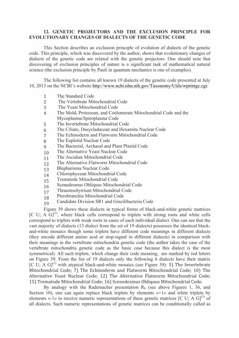
12. GENETIC PROJECTORS AND THE EXCLUSION PRINCIPLE FOR EVOLUTIONARY CHANGES OF DIALECTS OF THE GENETIC CODE

This Section describes an exclusion principle of evolution of dialects of the genetic code. This principle, which was discovered by the author, shows that evolutionary changes of dialects of the genetic code are related with the genetic projectors. One should note that discovering of exclusion principles of nature is a significant task of mathematical natural science (the exclusion principle by Pauli in quantum mechanics is one of examples).

The following list contains all known 19 dialects of the genetic code presented at July 10, 2013 on the NCBI’s website http://www.ncbi.nlm.nih.gov/Taxonomy/Utils/wprintgc.cgi:

1 2 3 4 5 6 7 8 9 10 11 12 13 14 15 16 17 18 19

The Standard Code The Vertebrate Mitochondrial Code The Yeast Mitochondrial Code The Mold, Protozoan, and Coelenterate Mitochondrial Code and the Mycoplasma/Spiroplasma Code The Invertebrate Mitochondrial Code The Ciliate, Dasycladacean and Hexamita Nuclear Code The Echinoderm and Flatworm Mitochondrial Code The Euplotid Nuclear Code The Bacterial, Archaeal and Plant Plastid Code The Alternative Yeast Nuclear Code The Ascidian Mitochondrial Code The Alternative Flatworm Mitochondrial Code Blepharisma Nuclear Code Chlorophycean Mitochondrial Code Trematode Mitochondrial Code Scenedesmus Obliquus Mitochondrial Code Thraustochytrium Mitochondrial Code Pterobranchia Mitochondrial Code Candidate Division SR1 and Gracilibacteria Code

Figure 39 shows these dialects in typical forms of black-and-white genetic matrices [C U; A G](3), where black cells correspond to triplets with strong roots and white cells correspond to triplets with weak roots in cases of each individual dialect. One can see that the vast majority of dialects (13 dialect from the set of 19 dialects) possesses the identical black-and-white mosaics though some triplets have different code meanings in different dialects (they encode different amino acid or stop-signal in different dialects) in comparison with their meanings in the vertebrate mitochondria genetic code (the author takes the case of the vertebrate mitochondria genetic code as the basic case because this dialect is the most symmetrical). All such triplets, which change their code meaning, are marked by red letters on Figure 39. From the list of 19 dialects only the following 6 dialects have their matrix [C U; A G](3) with atypical black-and-white mosaics (see Figure 39): 5) The Invertebrate Mitochondrial Code; 7) The Echinoderm and Flatworm Mitochondrial Code; 10) The Alternative Yeast Nuclear Code; 12) The Alternative Flatworm Mitochondrial Code; 15) Trematode Mitochondrial Code; 16) Scenedesmus Obliquus Mitochondrial Code.

By analogy with the Rademacher presentation R8 (see above Figures 1, 36, and Section 10), one can again replace black triplets by elements «+1» and white triplets by elements «-1» to receive numeric representations of these genetic matrices [C U; A G](3) of all dialects. Such numeric representations of genetic matrices can be conditionally called as

«±1-represenations». The result is the following: this numeric ±1-representation of matrices [C U; A G](3) of every of 19 dialects is decomposed into a sum of 8 sparse (8*8)-matrices of «column projectors» (or «row projectors») (see Figure 39). It is connected with the fact that all cells on main diagonals of these numeric matrices contain only «+1» (see the theorem in Section 7). This general feature of all dialects is a consequence of the following phenomenologic fact: biological evolution never changes code meaning of 16 black triplets, which occupies (2*2)-sub-quadrants along the main diagonal of these matrices (CCC, CCU, CCA, CCG, CGC, CGU, CGA, CGG, GCC, GCU, GCA, GCG, GGC, GGU, GGA, GGG).

From the point of view of algebra of projection operators, the described facts mean that biologic evolution of dialects of the genetic code is connected with a condition of conservation of the numeric ±1-representation of the genetic matrix [C U; A G](3) as a sum of 8 column projectors (or 8 row projectors). In other words, algebra of projectors shows an existence of an algebraic invariant of biological evolution.

One can formulate here the phenomenologic exclusion principle for evolutionary changes of dialects of the genetic code: it is forbidden for biological evolution to violate a separation of the set of 64 triplets into two subsets of triplets with strong and weak roots (black and white triplets) in a such way that a black-and-white mosaic of the genetic matrix [C U; A G](3) in its «±1-representation» ceases to be a sum of 8 column projectors (or 8 row projectors).

The Vertebrate Mitochondrial Code: CCC Pro

CCU Pro

CUC Leu

CUU Leu

UCC Ser

UCU Ser

UUC Phe

UUU Phe

CCA Pro

CCG Pro

CUA Leu

CUG Leu

UCA Ser

UCG Ser

UUA Leu

UUG Leu

CAC His

CAU His

CGC Arg

CGU Arg

UAC Tyr

UAU Tyr

UGC Cys

UGU Cys

CAA Gln

CAG Gln

CGA Arg

CGG Arg

UAA Stop

UAG Stop

UGA Trp

UGG trp

ACC Thr

ACU Thr

AUC Ile

AUU Ile

GCC Ala

GCU Ala

GUC Val

GUU Val

ACA Thr

ACG Thr

AUA Met

AUG Met

GCA Ala

GCG Ala

GUA Val

GUG Val

AAC Asn

AAU Asn

AGC Ser

AGU Ser

GAC Asp

GAU Asp

GGC Gly

GGU Gly

AAA Lys

AAG Lys

AGA Stop

AGG Stop

GAA Glu

GAG Glu

GGA Gly

GGG Gly

The Standard Code:

CCC Pro

CCU Pro

CUC Leu

CUU Leu

UCC Ser

UCU Ser

UUC Phe

UUU Phe

CCA Pro

CCG Pro

CUA Leu

CUG Leu

UCA Ser

UCG Ser

UUA Leu

UUG Leu

CAC His

CAU His

CGC Arg

CGU Arg

UAC Tyr

UAU Tyr

UGC Cys

UGU Cys

CAA Gln

CAG Gln

CGA Arg

CGG Arg

UAA Stop

UAG Stop

UGA Stop

UGG trp

ACC Thr

ACU Thr

AUC Ile

AUU Ile

GCC Ala

GCU Ala

GUC Val

GUU Val

ACA Thr

ACG Thr

AUA Ile

AUG Met

GCA Ala

GCG Ala

GUA Val

GUG Val

AAC Asn

AAU Asn

AGC Ser

AGU Ser

GAC Asp

GAU Asp

GGC Gly

GGU Gly

AAA Lys

AAG Lys

AGA Arg

AGG Arg

GAA Glu

GAG Glu

GGA Gly

GGG Gly

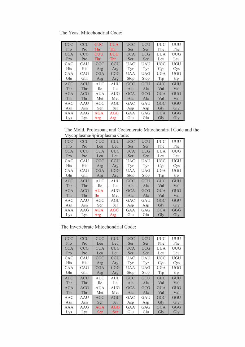
The Yeast Mitochondrial Code:

CCC Pro

CCU Pro

CUC Thr

CUA Thr

UCC Ser

UCU Ser

UUC Phe

UUU Phe

CCA Pro

CCG Pro

CUU Thr

CUG Thr

UCA Ser

UCG Ser

UUA Leu

UUG Leu

CAC His

CAU His

CGC Arg

CGU Arg

UAC Tyr

UAU Tyr

UGC Cys

UGU Cys

CAA Gln

CAG Gln

CGA Arg

CGG Arg

UAA Stop

UAG Stop

UGA Trp

UGG trp

ACC Thr

ACU Thr

AUC Ile

AUU Ile

GCC Ala

GCU Ala

GUC Val

GUU Val

ACA Thr

ACG Thr

AUA Met

AUG Met

GCA Ala

GCG Ala

GUA Val

GUG Val

AAC Asn

AAU Asn

AGC Ser

AGU Ser

GAC Asp

GAU Asp

GGC Gly

GGU Gly

AAA Lys

AAG Lys

AGA Arg

AGG Arg

GAA Glu

GAG Glu

GGA Gly

GGG Gly

The Mold, Protozoan, and Coelenterate Mitochondrial Code and the Mycoplasma/Spiroplasma Code:

CCC Pro

CCU Pro

CUC Leu

CUU Leu

UCC Ser

UCU Ser

UUC Phe

UUU Phe

CCA Pro

CCG Pro

CUA Leu

CUG Leu

UCA Ser

UCG Ser

UUA Leu

UUG Leu

CAC His

CAU His

CGC Arg

CGU Arg

UAC Tyr

UAU Tyr

UGC Cys

UGU Cys

CAA Gln

CAG Gln

CGA Arg

CGG Arg

UAA Stop

UAG Stop

UGA Trp

UGG trp

ACC Thr

ACU Thr

AUC Ile

AUU Ile

GCC Ala

GCU Ala

GUC Val

GUU Val

ACA Thr

ACG Thr

AUA Ile

AUG Met

GCA Ala

GCG Ala

GUA Val

GUG Val

AAC Asn

AAU Asn

AGC Ser

AGU Ser

GAC Asp

GAU Asp

GGC Gly

GGU Gly

AAA Lys

AAG Lys

AGA Arg

AGG Arg

GAA Glu

GAG Glu

GGA Gly

GGG Gly

The Invertebrate Mitochondrial Code:

CCC Pro

CCU Pro

CUC Leu

CUU Leu

UCC Ser

UCU Ser

UUC Phe

UUU Phe

CCA Pro

CCG Pro

CUA Leu

CUG Leu

UCA Ser

UCG Ser

UUA Leu

UUG Leu

CAC His

CAU His

CGC Arg

CGU Arg

UAC Tyr

UAU Tyr

UGC Cys

UGU Cys

CAA Gln

CAG Gln

CGA Arg

CGG Arg

UAA Stop

UAG Stop

UGA Trp

UGG trp

ACC Thr

ACU Thr

AUC Ile

AUU Ile

GCC Ala

GCU Ala

GUC Val

GUU Val

ACA Thr

ACG Thr

AUA Met

AUG Met

GCA Ala

GCG Ala

GUA Val

GUG Val

AAC Asn

AAU Asn

AGC Ser

AGU Ser

GAC Asp

GAU Asp

GGC Gly

GGU Gly

AAA Lys

AAG Lys

AGA Ser

AGG Ser

GAA Glu

GAG Glu

GGA Gly

GGG Gly

The Ciliate, Dasycladacean and Hexamita Nuclear Code:

CCC Pro

CCU Pro

CUC Leu

CUU Leu

UCC Ser

UCU Ser

UUC Phe

UUU Phe

CCA Pro

CCG Pro

CUA Leu

CUG Leu

UCA Ser

UCG Ser

UUA Leu

UUG Leu

CAC His

CAU His

CGC Arg

CGU Arg

UAC Tyr

UAU Tyr

UGC Cys

UGU Cys

CAA Gln

CAG Gln

CGA Arg

CGG Arg

UAA Gln

UAG Gln

UGA Stop

UGG trp

ACC Thr

ACU Thr

AUC Ile

AUU Ile

GCC Ala

GCU Ala

GUC Val

GUU Val

ACA Thr

ACG Thr

AUA Ile

AUG Met

GCA Ala

GCG Ala

GUA Val

GUG Val

AAC Asn

AAU Asn

AGC Ser

AGU Ser

GAC Asp

GAU Asp

GGC Gly

GGU Gly

AAA Lys

AAG Lys

AGA Arg

AGG Arg

GAA Glu

GAG Glu

GGA Gly

GGG Gly

The Echinoderm and Flatworm Mitochondrial Code:

CCC Pro

CCU Pro

CUC Leu

CUU Leu

UCC Ser

UCU Ser

UUC Phe

UUU Phe

CCA Pro

CCG Pro

CUA Leu

CUG Leu

UCA Ser

UCG Ser

UUA Leu

UUG Leu

CAC His

CAU His

CGC Arg

CGU Arg

UAC Tyr

UAU Tyr

UGC Cys

UGU Cys

CAA Gln

CAG Gln

CGA Arg

CGG Arg

UAA Stop

UAG Stop

UGA Trp

UGG trp

ACC Thr

ACU Thr

AUC Ile

AUU Ile

GCC Ala

GCU Ala

GUC Val

GUU Val

ACA Thr

ACG Thr

AUA Ile

AUG Met

GCA Ala

GCG Ala

GUA Val

GUG Val

AAC Asn

AAU Asn

AGC Ser

AGU Ser

GAC Asp

GAU Asp

GGC Gly

GGU Gly

AAA Asn

AAG Lys

AGA Ser

AGG Ser

GAA Glu

GAG Glu

GGA Gly

GGG Gly

The Euplotid Nuclear Code:

CCC Pro

CCU Pro

CUC Leu

CUU Leu

UCC Ser

UCU Ser

UUC Phe

UUU Phe

CCA Pro

CCG Pro

CUA Leu

CUG Leu

UCA Ser

UCG Ser

UUA Leu

UUG Leu

CAC His

CAU His

CGC Arg

CGU Arg

UAC Tyr

UAU Tyr

UGC Cys

UGU Cys

CAA Gln

CAG Gln

CGA Arg

CGG Arg

UAA Stop

UAG Stop

UGA Cys

UGG trp

ACC Thr

ACU Thr

AUC Ile

AUU Ile

GCC Ala

GCU Ala

GUC Val

GUU Val

ACA Thr

ACG Thr

AUA Ile

AUG Met

GCA Ala

GCG Ala

GUA Val

GUG Val

AAC Asn

AAU Asn

AGC Ser

AGU Ser

GAC Asp

GAU Asp

GGC Gly

GGU Gly

AAA Lys

AAG Lys

AGA Arg

AGG Arg

GAA Glu

GAG Glu

GGA Gly

GGG Gly

The Bacterial, Archaeal and Plant Plastid Code:

CCC Pro

CCU Pro

CUC Leu

CUU Leu

UCC Ser

UCU Ser

UUC Phe

UUU Phe

CCA Pro

CCG Pro

CUA Leu

CUG Leu

UCA Ser

UCG Ser

UUA Leu

UUG Leu

CAC His

CAU His

CGC Arg

CGU Arg

UAC Tyr

UAU Tyr

UGC Cys

UGU Cys

CAA Gln

CAG Gln

CGA Arg

CGG Arg

UAA Stop

UAG Stop

UGA Stop

UGG trp

ACC Thr

ACU Thr

AUC Ile

AUU Ile

GCC Ala

GCU Ala

GUC Val

GUU Val

ACA Thr

ACG Thr

AUA Ile

AUG Met

GCA Ala

GCG Ala

GUA Val

GUG Val

AAC Asn

AAU Asn

AGC Ser

AGU Ser

GAC Asp

GAU Asp

GGC Gly

GGU Gly

AAA Lys

AAG Lys

AGA Arg

AGG Arg

GAA Glu

GAG Glu

GGA Gly

GGG Gly

The Alternative Yeast Nuclear Code:

CCC Pro

CCU Pro

CUC Leu

CUU Leu

UCC Ser

UCU Ser

UUC Phe

UUU Phe

CCA Pro

CCG Pro

CUA Leu

CUG Ser

UCA Ser

UCG Ser

UUA Leu

UUG Leu

CAC His

CAU His

CGC Arg

CGU Arg

UAC Tyr

UAU Tyr

UGC Cys

UGU Cys

CAA Gln

CAG Gln

CGA Arg

CGG Arg

UAA Stop

UAG Stop

UGA Stop

UGG trp

ACC Thr

ACU Thr

AUC Ile

AUU Ile

GCC Ala

GCU Ala

GUC Val

GUU Val

ACA Thr

ACG Thr

AUA Ile

AUG Met

GCA Ala

GCG Ala

GUA Val

GUG Val

AAC Asn

AAU Asn

AGC Ser

AGU Ser

GAC Asp

GAU Asp

GGC Gly

GGU Gly

AAA Lys

AAG Lys

AGA Arg

AGG Arg

GAA Glu

GAG Glu

GGA Gly

GGG Gly

The Ascidian Mitochondrial Code:

CCC Pro

CCU Pro

CUC Leu

CUU Leu

UCC Ser

UCU Ser

UUC Phe

UUU Phe

CCA Pro

CCG Pro

CUA Leu

CUG Leu

UCA Ser

UCG Ser

UUA Leu

UUG Leu

CAC His

CAU His

CGC Arg

CGU Arg

UAC Tyr

UAU Tyr

UGC Cys

UGU Cys

CAA Gln

CAG Gln

CGA Arg

CGG Arg

UAA Stop

UAG Stop

UGA Trp

UGG trp

ACC Thr

ACU Thr

AUC Ile

AUU Ile

GCC Ala

GCU Ala

GUC Val

GUU Val

ACA Thr

ACG Thr

AUA Met

AUG Met

GCA Ala

GCG Ala

GUA Val

GUG Val

AAC Asn

AAU Asn

AGC Ser

AGU Ser

GAC Asp

GAU Asp

GGC Gly

GGU Gly

AAA Lys

AAG Lys

AGA Gly

AGG Gly

GAA Glu

GAG Glu

GGA Gly

GGG Gly

The Alternative Flatworm Mitochondrial Code:

CCC Pro

CCU Pro

CUC Leu

CUU Leu

UCC Ser

UCU Ser

UUC Phe

UUU Phe

CCA Pro

CCG Pro

CUA Leu

CUG Leu

UCA Ser

UCG Ser

UUA Leu

UUG Leu

CAC His

CAU His

CGC Arg

CGU Arg

UAC Tyr

UAU Tyr

UGC Cys

UGU Cys

CAA Gln

CAG Gln

CGA Arg

CGG Arg

UAA Stop

UAG Stop

UGA Trp

UGG trp

ACC Thr

ACU Thr

AUC Ile

AUU Ile

GCC Ala

GCU Ala

GUC Val

GUU Val

ACA Thr

ACG Thr

AUA Ile

AUG Met

GCA Ala

GCG Ala

GUA Val

GUG Val

AAC Asn

AAU Asn

AGC Ser

AGU Ser

GAC Asp

GAU Asp

GGC Gly

GGU Gly

AAA Asn

AAG Lys

AGA Ser

AGG Ser

GAA Glu

GAG Glu

GGA Gly

GGG Gly

Blepharisma Nuclear Code:

CCC Pro

CCU Pro

CUC Leu

CUU Leu

UCC Ser

UCU Ser

UUC Phe

UUU Phe

CCA Pro

CCG Pro

CUA Leu

CUG Leu

UCA Ser

UCG Ser

UUA Leu

UUG Leu

CAC His

CAU His

CGC Arg

CGU Arg

UAC Tyr

UAU Tyr

UGC Cys

UGU Cys

CAA Gln

CAG Gln

CGA Arg

CGG Arg

UAA Stop

UAG Gln

UGA Stop

UGG trp

ACC Thr

ACU Thr

AUC Ile

AUU Ile

GCC Ala

GCU Ala

GUC Val

GUU Val

ACA Thr

ACG Thr

AUA Ile

AUG Met

GCA Ala

GCG Ala

GUA Val

GUG Val

AAC Asn

AAU Asn

AGC Ser

AGU Ser

GAC Asp

GAU Asp

GGC Gly

GGU Gly

AAA Lys

AAG Lys

AGA Arg

AGG Arg

GAA Glu

GAG Glu

GGA Gly

GGG Gly

Chlorophycean Mitochondrial Code:

CCC Pro

CCU Pro

CUC Leu

CUU Leu

UCC Ser

UCU Ser

UUC Phe

UUU Phe

CCA Pro

CCG Pro

CUA Leu

CUG Leu

UCA Ser

UCG Ser

UUA Leu

UUG Leu

CAC His

CAU His

CGC Arg

CGU Arg

UAC Tyr

UAU Tyr

UGC Cys

UGU Cys

CAA Gln

CAG Gln

CGA Arg

CGG Arg

UAA Stop

UAG Leu

UGA Stop

UGG trp

ACC Thr

ACU Thr

AUC Ile

AUU Ile

GCC Ala

GCU Ala

GUC Val

GUU Val

ACA Thr

ACG Thr

AUA Ile

AUG Met

GCA Ala

GCG Ala

GUA Val

GUG Val

AAC Asn

AAU Asn

AGC Ser

AGU Ser

GAC Asp

GAU Asp

GGC Gly

GGU Gly

AAA Lys

AAG Lys

AGA Arg

AGG Arg

GAA Glu

GAG Glu

GGA Gly

GGG Gly

Trematode Mitochondrial Code: CCC Pro

CCU Pro

CUC Leu

CUU Leu

UCC Ser

UCU Ser

UUC Phe

UUU Phe

CCA Pro

CCG Pro

CUA Leu

CUG Leu

UCA Ser

UCG Ser

UUA Leu

UUG Leu

CAC His

CAU His

CGC Arg

CGU Arg

UAC Tyr

UAU Tyr

UGC Cys

UGU Cys

CAA Gln

CAG Gln

CGA Arg

CGG Arg

UAA Stop

UAG Stop

UGA Trp

UGG trp

ACC Thr

ACU Thr

AUC Ile

AUU Ile

GCC Ala

GCU Ala

GUC Val

GUU Val

ACA Thr

ACG Thr

AUA Met

AUG Met

GCA Ala

GCG Ala

GUA Val

GUG Val

AAC Asn

AAU Asn

AGC Ser

AGU Ser

GAC Asp

GAU Asp

GGC Gly

GGU Gly

AAA Asn

AAG Lys

AGA Ser

AGG Ser

GAA Glu

GAG Glu

GGA Gly

GGG Gly

Scenedesmus Obliquus Mitochondrial Code:

CCC Pro

CCU Pro

CUC Leu

CUU Leu

UCC Ser

UCU Ser

UUC Phe

UUU Phe

CCA Pro

CCG Pro

CUA Leu

CUG Leu

UCA Stop

UCG Ser

UUA Leu

UUG Leu

CAC His

CAU His

CGC Arg

CGU Arg

UAC Tyr

UAU Tyr

UGC Cys

UGU Cys

CAA Gln

CAG Gln

CGA Arg

CGG Arg

UAA Stop

UAG Leu

UGA Stop

UGG trp

ACC Thr

ACU Thr

AUC Ile

AUU Ile

GCC Ala

GCU Ala

GUC Val

GUU Val

ACA Thr

ACG Thr

AUA Ile

AUG Met

GCA Ala

GCG Ala

GUA Val

GUG Val

AAC Asn

AAU Asn

AGC Ser

AGU Ser

GAC Asp

GAU Asp

GGC Gly

GGU Gly

AAA Lys

AAG Lys

AGA Arg

AGG Arg

GAA Glu

GAG Glu

GGA Gly

GGG Gly

Thraustochytrium Mitochondrial Code:

CCC Pro

CCU Pro

CUC Leu

CUU Leu

UCC Ser

UCU Ser

UUC Phe

UUU Phe

CCA Pro

CCG Pro

CUA Leu

CUG Leu

UCA Ser

UCG Ser

UUA Stop

UUG Leu

CAC His

CAU His

CGC Arg

CGU Arg

UAC Tyr

UAU Tyr

UGC Cys

UGU Cys

CAA Gln

CAG Gln

CGA Arg

CGG Arg

UAA Stop

UAG Stop

UGA Stop

UGG trp

ACC Thr

ACU Thr

AUC Ile

AUU Ile

GCC Ala

GCU Ala

GUC Val

GUU Val

ACA Thr

ACG Thr

AUA Ile

AUG Met

GCA Ala

GCG Ala

GUA Val

GUG Val

AAC Asn

AAU Asn

AGC Ser

AGU Ser

GAC Asp

GAU Asp

GGC Gly

GGU Gly

AAA Lys

AAG Lys

AGA Arg

AGG Arg

GAA Glu

GAG Glu

GGA Gly

GGG Gly

Pterobranchia Mitochondrial Code:

CCC Pro

CCU Pro

CUC Leu

CUU Leu

UCC Ser

UCU Ser

UUC Phe

UUU Phe

CCA Pro

CCG Pro

CUA Leu

CUG Leu

UCA Ser

UCG Ser

UUA Leu

UUG Leu

CAC His

CAU His

CGC Arg

CGU Arg

UAC Tyr

UAU Tyr

UGC Cys

UGU Cys

CAA Gln

CAG Gln

CGA Arg

CGG Arg

UAA Stop

UAG Stop

UGA Trp

UGG trp

ACC Thr

ACU Thr

AUC Ile

AUU Ile

GCC Ala

GCU Ala

GUC Val

GUU Val

ACA Thr

ACG Thr

AUA Ile

AUG Met

GCA Ala

GCG Ala

GUA Val

GUG Val

AAC Asn

AAU Asn

AGC Ser

AGU Ser

GAC Asp

GAU Asp

GGC Gly

GGU Gly

AAA Lys

AAG Lys

AGA Ser

AGG Lys

GAA Glu

GAG Glu

GGA Gly

GGG Gly

Candidate Division SR1 and Gracilibacteria Code:

CCC Pro

CCU Pro

CUC Leu

CUU Leu

UCC Ser

UCU Ser

UUC Phe

UUU Phe

CCA Pro

CCG Pro

CUA Leu

CUG Leu

UCA Ser

UCG Ser

UUA Leu

UUG Leu

CAC His

CAU His

CGC Arg

CGU Arg

UAC Tyr

UAU Tyr

UGC Cys

UGU Cys

CAA Gln

CAG Gln

CGA Arg

CGG Arg

UAA Stop

UAG Stop

UGA Gly

UGG trp

ACC Thr

ACU Thr

AUC Ile

AUU Ile

GCC Ala

GCU Ala

GUC Val

GUU Val

ACA Thr

ACG Thr

AUA Ile

AUG Met

GCA Ala

GCG Ala

GUA Val

GUG Val

AAC Asn

AAU Asn

AGC Ser

AGU Ser

GAC Asp

GAU Asp

GGC Gly

GGU Gly

AAA Lys

AAG Lys

AGA Arg

AGG Arg

GAA Glu

GAG Glu

GGA Gly

GGG Gly

Figure 39. The matrices [C U; A G](3) show 19 known dialects of the genetic code. Black (white) cells contain triplets with strong (weak) roots. Red color shows triplets, which have different code meanings in a considered dialect in comparison with their code meanings in the Vertebrate Mitochondrial Code, which is the most symmetrical among all dialects.

13. ABOUT «TENSORCOMPLEX» NUMBERS

This Section describes a system of multidimensional numbers, which seem to be a new one for mathematical natural sciences and which are constructed on the basis of sums of genetic projectors described above. Here the author will take some data from his work [Petoukhov, 2012b]. First of all, let us return to two sums of genetic projectors h0+h2 and h1+h3 (from Figure 10), which were received from the Hadamard matrix H4 (Figure 1). The first sum h0+h2 is decomposed into two basic matrices e0 = [1 0 0 0; -1 0 0 0; 0 0 1 0; 0 0 -1 0] and e2 = [0 0 -1 0; 0 0 1 0; 1 0 0 0; -1 0 0 0], the set of which is closed relative to multiplication and defines the multiplication table of complex numbers. The second sum h1+h3 is decomposed into other basic matrices e1 = [0 1 0 0; 0 1 0 0; 0 0 0 1; 0 0 0 1] and e3 = [0 0 0 1; 0 0 0 1;

0 -1 0 0; 0 -1 0 0], the set of which is closed relative to multiplication and also defines the multiplication table of complex numbers (see Figure 10). Now one can consider linear compositions CL and GR on basis of these basic matrices (Figure 37, upper level). The work [Petoukhov, 2012b] shows that each of CL and CR is a (4*4)-matrix representation of 2-parametric complex numbers over field of real numbers but these representations concern different 2-dimensional planes (x0, x2) and (x1, x3) of a 4-dimensional vector space.

Many people know that the sum of two complex numbers gives a new complex number and that the product of two complex numbers is commutative. This is true when these complex numbers belong to the same complex plane. But the sum of these (4x4)-representations of two complex numbers CL and CR, which belong to different planes of 4-dimensional space, is not equal to a new complex number, and their product is not commutative: CL*CR ≠ CR*CL. Each of these products CL*CR and CR*CL gives a new complex number. Figure 40 (two middle levels) show expressions CL*CR and CR*CL with their decompositions into sets of two matrices, which correspond to the multiplication table of complex numbers. Figure 40 (bottom level) also shows an expression of a corresponding commutator. One should note here that the expression of the commutator CL*CR-CR*CL on Figure 40 belongs to so called “tensorcomplex numbers”, which will be introduced below (Figures 41 and 42) with marks of their quadrants by means of yellow and green colors to emphasise a special cross-like structure of this type of numbers.

CL=a0*e0+a2*e2=

a0 0 -‐a2 0 ; CR=a1*e1+a3*e3=

0 a1 0 a3 -‐a0 0 a2 0 0 a1 0 a3 a2 0 a0 0 0 -‐a3 0 a1 -‐a2 0 -‐a0 0 0 -‐a3 0 a1

CL*CR=

0, a0*a1+a2*a3, 0, a0*a3-a1*a2 0, -a0*a1-a2*a3, 0, a1*a2-a0*a3 0, a1*a2-a0*a3, 0, a0*a1+a2*a3 0, a0*a3-a1*a2, 0, -a0*a1-a2*a3

= -(a0*a1+a2*a3)*

0 -1 0 0 0 1 0 0 0 0 0 -1 0 0 0 1

+(a1*a2-a0*a3)*

0 0 0 -1 0 0 0 1 0 1 0 0 0 -1 0 0

CR*CL=

-a0*a1-a2*a3, 0, a1*a2-a0*a3, 0 -a0*a1-a2*a3, 0, a1*a2-a0*a3, 0 a0*a3-a1*a2, 0, -a0*a1-a2*a3, 0 a0*a3-a1*a2, 0, -a0*a1-a2*a3, 0

=-(a0*a1+a2*a3)*

1 0 0 0 1 0 0 0 0 0 1 0 0 0 1 0

- ( a1*a2-a0*a3)*

0 0 -1 0 0 0 -1 0 1 0 0 0 1 0 0 0

CL*CR-CR*CL=

a0*a1+a2*a3, a0*a1+a2*a3 a0*a1+a2*a3, -a0*a1-a2*a3

a0*a3-a1*a2, a0*a3-a1*a2 a0*a3-a1*a2, a1*a2-a0*a3

a1*a2-a0*a3, a1*a2-a0*a3 a1*a2-a0*a3, a0*a3-a1*a2

a0*a1+a2*a3, a0*a1+a2*a3 a0*a1+a2*a3, -a0*a1-a2*a3

Figure 40. Upper level: CL is a (4*4)-matrix representation of complex numbers z = a0 + a2*i on a 2-dimensional plane (x0, x2) in a 4-dimensional space (x0, x1, x2, x3); here i is imaginary unit of complex numbers (i2 = -1). CR is a (4*4)-matrix representation of complex numbers z = a1 + a3*i on another 2-dimensional plane (x1, x3) in the same 4-dimensional space (x0, x1, x2, x3). Here a0, a1, a2 and a3 are real numbers. Two middle levels: expressions of products CL*CR and CR*CL; in both cases two basic matrices define the multiplication table of complex numbers. Bottom level: the expression of the commutator CL*CR-CR*CL.

Now let us take a sum V = CL + CR of these (4*4)-matrix representations of complex numbers, which are related with different planes of the 4-dimensional space (Figure 41).

V = CL + CR =

a0 a1 -‐a2 a3 = [1 0; 0 1]UM + [0 1; -‐1 0]UP -‐a0 a1 a2 a3

a2 -‐a3 a0 a1 -‐a2 -‐a3 -‐a0 a1

V-1 = (2*(a0

2 + a22))-1 *

a0 -a0 a2 -a2 + (2*(a1

2 + a32))-1 *

0 0 0 0 0 0 0 0 a1 a1 -a3 -a3 -a2 a2 a0 -a0 0 0 0 0 0 0 0 0 a3 a3 a1 a1

Figure 41. Upper level: the sum V = CL + CR (see Figure 40). Here M=[a0 a1; -a0 a1] and P=[-a2 a3; a2 a3]; U is a symbol of tensor (or Kronecker) multiplication. Bottom level: the expression of the inverse matrix V-1.

Figure 41 shows that V=CL+CR is a (4*4)-matrix of a special type, where both quadrants (marked by yellow color) along the main diagonal are identical each other, and two other quadrants (marked by green color) differ each from other only by inversion of sign in their entries. This matrix can be written in a form V = [1 0; 0 1]UM + [0 1; -1 0]UP, where M=[a0 a1; -a0 a1] and P=[-a2 a3; a2 a3]; U is a symbol of tensor multiplication; [1 0; 0 1] – a matrix representation of real unit; [0 1; -1 0] – a matrix representation of imaginary unit; a0, a1, a2 and a3 are real numbers. Such form of denotation resembles a well-known matrix representation of usual complex numbers: z = [1 0; 0 1]*a + [0 1; -1 0]*b, where a and b are real numbers. But it differs in the following aspects:

1) the expression V = [1 0; 0 1]UM + [0 1; -1 0]UP includes tensor multiplication U instead of usual multiplication in the matrix representation of complex numbers;

2) in the case of V, multipliers of the basic elements are square matrices M and P instead of real numbers «a» and «b» in the case of complex numbers.

3) The order of the factors inside V is essential since tensor multiplication is not commutative.

Let us consider a set of matrices, which includes all matrices of this kind V together with their inverse matrices V-1 and together with all products of matrices of this kind. This set of matrices has properties of multi-dimensional numeric system as it is described below.

What one can say about algebraic properties of matrices of such type V (Figure 41)? Matrices of this type can be added and subtracted. The matrix V has its inverse matrix V-1 (Figure 42), which is defined on the basis of the condition V*V-1=V-1*V=E4, where E4 is identity matrix [1 0 0 0; 0 1 0 0; 0 0 1 0; 0 0 0 1]. Product of two different matrices of this type (for example G and S on Figure 42) generates a new (4*4)-matrix W=G*S (Figure 42), where both (2*2)-quadrants (marked by yellow color) along the main diagonal are identical each other, and two other (2*2)-quadrants (marked by green color) differ each from other only by inversion of sign in their entries. This matrix can be written in a form W = [1 0; 0 1]UQ + [0 1; -1 0]UK, where Q=[ a*k-c*k-b*n-d*n, a*m+c*m+b*p-d*p; b*n-c*k-a*k-d*n, c*m-a*m-b*p-d*p] and K=[c*n-a*n-d*k-b*k, a*p-b*m+d*m+c*p; b*k+a*n-d*k+c*n,

b*m-a*p+d*m+c*p]; U is a symbol of tensor multiplication; [1 0; 0 1] – a matrix representation of real unit; [0 1; -1 0] – a matrix representation of imaginary unit; a, b, c, d, k, m, n and p are real numbers. Such form of denotation resembles the known matrix representation of usual complex numbers: z = [1 0; 0 1]*a + [0 1; -1 0]*b, where a and b are real numbers. But it differs again in the following aspects:

1) the expression W = [1 0; 0 1]UQ + [0 1; -1 0]UK includes tensor multiplication U instead of usual multiplication in the matrix representation of complex numbers;

2) in the case of W, multipliers of the basic elements are square matrices Q and K instead of real numbers «a» and «b» in the case of complex numbers.

3) The order of the factors inside W is essential since tensor multiplication is not commutative.

Taking into account a significant role of tensor multiplication U in W, the author names algebraic constructions in a form W as “tensorcomplex numbers” because such matrices W have the following algebraic properties in relation to usual operations of addition, subtraction, multiplication and division:

• Addition and subtraction of two different matrices of this type W create a new matrix of the same type. Multiplication of different matrices of this type with each other is noncommutative and it gives a new matrix of the same type (Figure 42).

• Each non-zero matrix W=G*S has an inverse matrix W-1 = G-1*S-1 (expressions for G-1 and S-1 were shown on Figure 41). It allows a definition of operation of division of two matrices of this type as a multiplication with an inverse matrix.

Such properties of tensorcomplex numbers resemble algebraic properties of quaternions by Hamilton, which represent noncommutative division algebra (http://en.wikipedia.org/wiki/Quaternion). Here one should emphasize that tensorcomplex numbers cardinally differ from hypercomplex numbers x0+x1*i1+…+xn*in, where x0, x1,…, xn are real numbers, because, in the case of tensorcomplex numbers, multipliers of the basic elements are square matrices but not real numbers. By this reason, the famous Frobenius theorem (http://en.wikipedia.org/wiki/Frobenius_theorem_(real_division_algebras)) for hypercomplex numbers is not related to tensorcomplex numbers. This theorem says that any finite-dimensional associative division algebra is isomorphic to one of the following algebras: the real numbers, the complex numbers, the quaternions by Hamilton.

G=

a c -b d ; S =

k m -n p -a c b d -k m n p b -d a c n -p k m -b -d -a c -n -p -k m

G*S=

a*k-c*k-b*n-d*n a*m+c*m+b*p-d*p c*n-a*n-d*k-b*k a*p-b*m+d*m+c*p b*n-c*k-a*k-d*n c*m-a*m-b*p-d*p b*k+a*n-d*k +c*n b*m-a*p+d*m+c*p b*k+a*n+d*k-c*n b*m-a*p-d*m-c*p a*k-c*k-b*n-d*n a*m+c*m+b*p-d*p d*k-a*n-b*k-c*n a*p-b*m-d*m-c*p b*n-c*k-a*k-d*n c*m-a*m-b*p-d*p

Figure 42. Multiplication of two matrices G and S gives a new matrix W = G*S, which belong to so called «tensorcomplex numbers». Here a, b, c, d, k, m, n and p are real numbers.

This set of tensorcomplex numbers is one of examples of numeric systems, where real numbers exist only inside matrices in a form of whole ensembles but not as individual multipliers (or as individual personages) inside such numeric systems. It is one of differences of tensorcomplex numbers from hypercomplex systems. One can mention that the commutator CL*CR-‐CR*CL (Figure 40) belongs to tensorcomplex numbers. Till now in this Section we considered the case of tensorcomplex numbers, which were represented by means of the expression W = [1 0; 0 1]UQ + [0 1; -1 0]UK, where Q and K are (2*2)-matrices. But our work [Petoukhov, 2012b,….] describes that complex numbers can be also represented by means of sparse (2N*2N)-matrices on the basis of sums of projectors (here N = 2, 3, 4, …). One can take sum of two complex numbers, which belong to different planes of the same 2N-dimensional space and which are represented by means of appropriate (2N*2N)-matrices. In this case new types of tensorcomplex numbers arise. Theory and expressions for such tensorcomplex numbers in spaces of higher dimensions are developed now for a publication in the nearest future. The author hopes that tensorcomplex numbers, which seem to be a new type of multidimensional numbers for mathematical natural sciences, will be useful not only in bioinformatics, but also in physics, theory of communication, logic and other fields.

14. ABOUT «TENSORHYPERBOLIC» NUMBERS

Now let us return to the Rademacher (4*4)-matrix R4, which is a sum of 4 column projectors c0, c1, c2, c3: R4 = c0+c1+c2+c3 (Figures 1 and 2). Our work [Petoukhov, 2012b, Figures 11-13] shows that sum c0+c2 is decomposed into basic matrices e0 = [1 0 0 0; -1 0 0 0; 0 0 1 0; 0 0 -1 0] and e2 = [0 0 1 0; 0 0 -1 0; 1 0 0 0; -1 0 0 0], the set of which is closed relative to multiplication and defines the multiplication table of hyperbolic numbers; their known synonyms are “split-complex numbers”, “double numbers” or “Lorentz numbers” (http://en.wikipedia.org/wiki/Split-complex_number). In this paper we will prefer using the name «hyperbolic numbers» for such type of 2-dimensional numbers. Another sum c1+c3 is decomposed into basic matrices e1 = [0 1 0 0; 0 1 0 0; 0 0 0 1; 0 0 0 1] and e3 = [0 0 0 -1; 0 0 0 -1; 0 -1 0 0; 0 -1 0 0]. Now one can consider linear compositions DL and DR on basis of these basic matrices (Figure 43). The work [Petoukhov, 2012b, Figures 12, 13] shows that each of DL and DR is a (4*4)-matrix representation of 2-parametric hyperbolic numbers over field of real numbers but these representations concern different 2-dimensional planes (x0, x2) and (x1, x3) of a 4-dimensional vector space.

DL=a0*e0+a2*e2=

a0 0 a2 0 ; DR=a1*e1+a3*e3=

0 a1 0 -‐a3 -‐a0 0 -‐a2 0 0 a1 0 -‐a3 a2 0 a0 0 0 -‐a3 0 a1 -‐a2 0 -‐a0 0 0 -‐a3 0 a1

Figure 43. Left side: DL is a (4*4)-matrix representation of hyperbolic (or split-complex) numbers z = a0 + a2*j on a 2-dimensional plane (x0, x2) in a 4-dimensional space (x0, x1, x2, x3); here j is imaginary unit of hyperbolic numbers (j2=1). Right side: DR is a (4*4)-matrix representation of hyperbolic numbers z = a1 + a3*j on another 2-dimensional plane (x1, x3) in the same 4-dimensional space (x0, x1, x2, x3). Here a0, a1, a2 and a3 are real numbers.

Now let us take a sum DL+DR of these (4*4)-‐matrix representations of hyperbolic numbers, which are related with different planes of the 4-‐dimensional space (Figure 44).

D = DL + DR =

a0 a1 a2 -‐a3 = [1 0; 0 1]UM + [0 1; 1 0]UK -‐a0 a1 -‐a2 -‐a3

a2 -‐a3 a0 a1 -‐a2 -‐a3 -‐a0 a1

a 0 a 0 -‐a 0 a 0 a 0 a 0 -‐a 0 -‐a 0

*

0 c 0 -‐c 0 c 0 -‐c 0 -‐c 0 c 0 -‐c 0 c

=

0 0 0 0 0 0 0 0 0 0 0 0 0 0 0 0

D-‐1 = (2*(a02 – a22))-‐1 *

a0 -‐a0 -‐a2 a2 0 0 0 0 -‐a2 a2 a0 -‐a0 0 0 0 0

+ (2*(a12 – a32))-‐1 *

0 0 0 0 a1 a1 -‐a3 -‐a3 0 0 0 0 -‐a3 -‐a3 a1 a1

Figure 44. Upper level: the sum D = DL+DR (see Figure 43). Here M=[a0 a1; -‐a0 a1]

and K=[a2 -‐a3; -‐a2 -‐a3]; U is a symbol of tensor multiplication. Middle level: the example of zero divizors in this type of matrices. Bottom level: the inverse matix D-‐1. Figure 44 shows that D = DL+DR is a (4*4)-matrix of a special type, where both quadrants along each of diagonals are identical (they are marked by yellow and blue colors). This matrix can be written in a form D = [1 0; 0 1]UM + [0 1; 1 0]UK, where M=[a0 a1; -a0 a1] and K=[a2 -a3; -a2 -a3], where [1 0; 0 1] – a matrix representation of real unit; [0 1; 1 0] – a matrix representation of imaginary unit j of hyperbolic numbers (j2=1); a0, a1, a2 and a3 are real numbers. Such form of denotation resembles a well-known matrix representation of usual hyperbolic numbers: y = [1 0; 0 1]*a + [0 1; 1 0]*b, where «a» and «b» are real numbers. But it differs again in the following aspects:

1) the expression D = [1 0; 0 1]UM + [0 1; 1 0]UK includes tensor multiplication U instead of usual multiplication in the matrix representation of hyperbolic numbers;

2) in the case of D, multipliers of the basic elements are square matrices M and K instead of real numbers «a» and «b» in the case of hyperbolic numbers;

3) The order of factors inside D is essential since tensor multiplication is not commutative.

The set of matrix D has zero divisors, examples of which are shown on Figure 44. Figure 44 also shows a general expression of the inverse matrix D-1 for the matrix D.

Multiplication of two matrices D0 and D1 of this type gives a new matrix L (Figure 45), where both quadrants along each of diagonals are identical (they are marked by yellow and blue colors). This matrix can be represented in the following form: L = [1 0; 0 1]UQ + [0 1; 1 0]UK, where Q = [a*k-c*k+b*n+d*n, a*m+c*m-b*p+d*p; d*n-c*k-b*n-a*k, c*m-a*m +b*p +d*p], K=[a*n+b*k-c*n+d*k, b*m-a*p-c*p-d*m; d*k-b*k-c*n-a*n, a*p-b*m-c*p-d*m].

Taking into account a significant role of tensor multiplication U in L, the author names algebraic constructions in a form L (Figure 45) as “tensorhyperbolic numbers” because such matrices L have the following algebraic properties in relation to usual operations of addition, subtraction, multiplication and division:

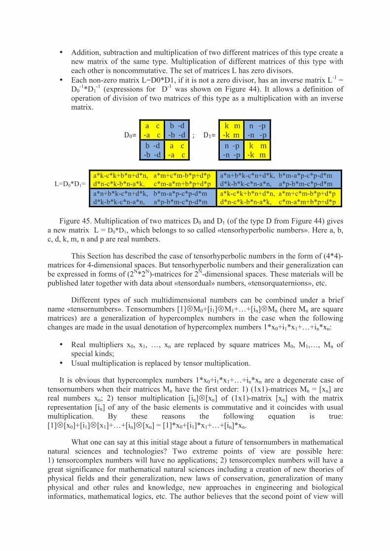
• Addition, subtraction and multiplication of two different matrices of this type create a new matrix of the same type. Multiplication of different matrices of this type with each other is noncommutative. The set of matrices L has zero divisors.

• Each non-zero matrix L=D0*D1, if it is not a zero divisor, has an inverse matrix L-1 = D0

-1*D1-1 (expressions for D-1 was shown on Figure 44). It allows a definition of

operation of division of two matrices of this type as a multiplication with an inverse matrix.

D0=

a c -‐a c

b -‐d -‐b -‐d

; D1=

k m -‐k m

n -‐p -‐n -‐p

b -‐d -‐b -‐d

a c -‐a c

n -‐p -‐n -‐p

k m -‐k m

L=D0*D1=

a*k-c*k+b*n+d*n, a*m+c*m-b*p+d*p d*n-c*k-b*n-a*k, c*m-a*m+b*p+d*p

a*n+b*k-c*n+d*k, b*m-a*p-c*p-d*m d*k-b*k-c*n-a*n, a*p-b*m-c*p-d*m

a*n+b*k-c*n+d*k, b*m-a*p-c*p-d*m d*k-b*k-c*n-a*n, a*p-b*m-c*p-d*m

a*k-c*k+b*n+d*n, a*m+c*m-b*p+d*p d*n-c*k-b*n-a*k, c*m-a*m+b*p+d*p

Figure 45. Multiplication of two matrices D0 and D1 (of the type D from Figure 44) gives a new matrix L = D0*D1, which belongs to so called «tensorhyperbolic numbers». Here a, b, c, d, k, m, n and p are real numbers.

This Section has described the case of tensorhyperbolic numbers in the form of (4*4)-matrices for 4-dimensional spaces. But tensorhyperbolic numbers and their generalization can be expressed in forms of (2N*2N)-matrices for 2N-dimensional spaces. These materials will be published later together with data about «tensordual» numbers, «tensorquaternions», etc.

Different types of such multidimensional numbers can be combined under a brief name «tensornumbers». Tensornumbers [1]UM0+[i1]UM1+…+[in]UMn (here Mn are square matrices) are a generalization of hypercomplex numbers in the case when the following changes are made in the usual denotation of hypercomplex numbers 1*x0+i1*x1+…+in*xn:

• Real multipliers x0, x1, …, xn are replaced by square matrices M0, M1,…, Mn of special kinds;

• Usual multiplication is replaced by tensor multiplication.

It is obvious that hypercomplex numbers 1*x0+i1*x1+…+in*xn are a degenerate case of tensornumbers when their matrices Mn have the first order: 1) (1x1)-matrices Mn = [xn] are real numbers xn; 2) tensor multiplication [in]U[xn] of (1x1)-matrix [xn] with the matrix representation [in] of any of the basic elements is commutative and it coincides with usual multiplication. By these reasons the following equation is true: [1]U[x0]+[i1]U[x1]+…+[in]U[xn] = [1]*x0+[i1]*x1+…+[in]*xn.

What one can say at this initial stage about a future of tensornumbers in mathematical natural sciences and technologies? Two extreme points of view are possible here: 1) tensorcomplex numbers will have no applications; 2) tensorcomplex numbers will have a great significance for mathematical natural sciences including a creation of new theories of physical fields and their generalization, new laws of conservation, generalization of many physical and other rules and knowledge, new approaches in engineering and biological informatics, mathematical logics, etc. The author believes that the second point of view will

coincide with a real future in a higher extent.

15. UNITED-HYPERCOMPLEX NUMBERS AND GENETIC MATRICES

As known, hypercomplex numbers have a single real unit and additional quantity of imaginary units, all of which in the total are called basic elements of hypercomplex numbers. The expression (10) shows their linear form of writing in general case:

a0*E + a1*e1 + a2*e2 + ……. + an*en (10)

where E denotes the real unit (or the identity matrix E in the case of the matrix representation of hypercomplex numbers), e1, e2, …, en denote imaginary units, a0, a1, …., an denote real coefficients. The set of these basic elements (E, e1, e2,…, en) should be closed under multiplication. This means that multiplication of any two basic elements with each other always gives again one of these elements or their linear superposition [Kantor, Solodovnikov, 1989].

In the result of our study of systems of structured alphabets of DNA and RNA in matrix forms of their Walsh-representations R4, R8, H4, H8 (Fig. 1) we have revealed that these alphabetic structures are connected with special (2n*2n)-matrix operators. Various decompositions of these operators show their connection with special 2n-dimensional numeric systems with the following features: 1) they are not hypercomplex numbers in the whole because of absence of the identity matrix E in their decompositions (that is the general real unit is absent among basic elements of such systems); 2) they contain two or more blocks, each of whose represents complex numbers or hypercomplex numbers with its individual set of basic elements, which play role of its individual real unit and imaginary units but only inside a separate block; by this reason we call them as local-real units and local-imaginary units. In other words, two or more different systems of complex or hypercomplex numbers exist in this case not separately but are united together into a single whole in a form of special block matrices. Multiplication tables (in cases of their existence) of basic elements of such systems have a character of plexus structures. The author calls such multi-dimensional numeric systems as "united-hypercomplex numeric systems" (or briefly, U-hypercomplex numbers or simply U-numbers). These united-hypercomplex numbers possess interesting properties to model biological phenomena and multi-parametrical systems in general. One can think that U-complex numbers and U-hypercomplex numbers play an important role in bioinformation phenomena since they are connected with the phenomenology of alphabets of DNA and RNA.

Let us consider the Walsh-representaion R4 (Fig. 1) of the matrix of 16 doublets [C, T; A, G](2). The matrix R4 can be decomposed into sum of 4 sparse matrices e0, e1, e2, e3, for example, in the way shown on Fig. 46. It is interesting that this variant of the decomposition consists of two sets of matrices, each of which is closed in relation to multiplication unexpectedly: the first set consists of matrices e0 and e1; the second set – matrices e2 and e3. Fig. 46 shows multiplication tables for both sets, in each of which multiplication between its elements always gives an element from the same set. These multiplication tables coincide with the multiplication table of basic elements of complex numbers.

1 1 1 -1 -1 1 -1 -1 1 -1 1 1 -1 -1 -1 1

=

1 0 0 0 0 1 0 0 0 -1 0 0 -1 0 0 0

+

0 1 0 0 -1 0 0 0 1 0 0 0 0 -1 0 0

+

0 0 0 -1 0 0 -1 0 0 0 1 0 0 0 0 1

+

0 0 1 0 0 0 0 -1 0 0 0 1 0 0 -1 0

= e0+e1+e2+e3

* e0 e1

e0 e0 e1

e1 e1 -e0

* e2 e3

e2 e2 e3

e3 e3 -e2

Fig. 46. Top: the decomposition of the matrix R4 (Fig. 1) into 4 sparse matrices e0, e1,

e2, e3. Bottom: multiplication tables of pairs of matrices e0 and e1 (left) and e2 and e3 (right) coincide with the multiplication table of basic elements of complex numbers.

It means that each of expressions ZL=a0*e0+a1*e1 and ZR=a2*e2+a3*e3 , where e0, e1, e2, e3 are taken from Fig. 46, represents its own system of complex numbers in the unusual form of the sparse (4*4)-matrix with their 2 independent parameters a0, a1 and a2, a3 correspondingly (Fig. 47). It can be formulated also in the following way: each of the systems ZL and ZR is isomorphic to the classical system of complex numbers. Inside the system ZL, the matrix e0+e1 represents the complex number with unit coordinates (a0=a1=1). Inside the system ZR, the matrix e2+e3 represents the complex number with unit coordinates (a2=a3=1).

ZL =

a0, a1, 0, 0 -a1, a0, 0, 0 a1, -a0, 0, 0 -a0, -a1, 0, 0

; ZL-1 = (a0

2+a12)-1 *

a0, -a1, 0, 0 a1, a0, 0, 0 -a1, -a0, 0, 0 -a0, a1, 0, 0

ZR =

0, 0, a3, -a2 0, 0, -a2, -a3 0, 0, a2, a3 0, 0, -a3, a2

; ZR-1 = (a2

2+a32)-1 *

0, 0, -a3, -a2 0, 0, -a2, a3 0, 0, a2, -a3 0, 0, a3, a2

Fig. 47. Left: two systems of complex numbers ZL=a0*e0+a1*e1 and ZR=a2*e2+a3*e3 in their form of (4*4)-matrices. Right: inverse matrices ZL-1 and ZR-1 in relation to matrices e0 and e2, which play the role of identity matrices in the systems ZL and ZR correspondingly.

The classical identity matrix E=[1 0 0 0; 0 1 0 0; 0 0 1 0; 0 0 0 1] is absent in the set of matrices ZL and ZR, where - beside this - each matrix has zero determinant. Consequently the usual notion of the inverse matrix ZL-1 or ZR-1 (as ZL*ZL-1=E or ZR*ZR-1 =E) can’t be defined in relation to the identity matrix E in accordance with the famous theorem about inverse matrices for matrices with zero determinant in the case of the complete set of matrices (Bellman, 1960, Chapter 6, § 4). But we analyze not the complete set of (4*4)-matrices but very limited special sets of matrices ZL and ZR. The system ZL has the matrix e0 (Fig. 46), which possesses all properties of the identity matrix for any matrix ZL since e0*ZL = ZL*e0 = ZL and e0

2 = e0. In the frame of the system of matrices ZL, where locally the matrix e0 plays the role of the identity matrix (the local-identity matrix), one can define - for any non-zero matrix ZL - its inverse matrix ZL-1 in relation to the matrix e0 on the basis of equations: ZL*ZL-1 = ZL-1*ZL = e0. (Fig. 47).

By analogy, the system of matrices ZR has the matrix e2 (Fig. 46), which possesses all properties of the identity matrix for any matrix ZR since e2*ZR = ZR*e2 = ZR and e2

2 = e2. In the frame of the system of matrices ZR, where locally the matrix e2 plays the role of the identity matrix (the local-identity matrix), one can define - for any non-zero matrix ZR - its inverse matrix ZR-1 in relation to the matrix e2 on the base of equations: ZR*ZR-1 = ZR-1*ZR = e2 (Fig. 47).

Multiplication of two members from the same system ZL (or ZR) is commutative as it is true for complex numbers. But multiplication of two members from different systems (one member from ZL and one member from ZR) is not commutative and gives a new matrix from one of these systems.

Multiplication of a complex number ZL=a0*e0+a1*e1 with its conjugate complex number a0*e0-a1*e1 gives the norm of this complex number: (a0

2+a12)*e0. Multiplication of a

complex number ZR=a2*e2+a3*e3 with its conjugate complex number a2*e2-a3*e3 gives the norm of this complex number: (a2

2+a32)*e2. Each of these norms can be called as a local-

norm inside the set of matrices Z2 = ZL+ZR = a0*e0+a1*e1+a2*e2+a3*e3. One should emphasized that the total set of sparse matrices e0, e1, e2, e3 does not

contain the identity matrix E=[1,0,0,0; 0,1,0,0; 0,0,1,0; 0,0,0,1] and therefore the total sum Z2=a0*e0+a1*e1+a2*e2+a3*e3 does not represent a system of hypercomplex numbers. It contains two blocks of complex numbers (a0*e0+a1*e1) and (a2*e2+a3*e3) and by this reason it is one of many types of U-complex numbers. It can be called as the 2-block U-complex numeric system (other U-complex systems can include more quantity of blocks as shown below). The set of its basic elements is closed under multiplication and defines the multiplication table in Fig. 48. In the system of U-complex numbers Z2, the matrices e0 and e1 are conditionally called as the local-real unit and the local-imaginary unit correspondingly in the block ZL=a0*e0+a1*e1; the matrices e2 and e3 are called as the local-real unit and the local-imaginary unit in the block ZR=a2*e2+a3*e3.

Z2 = ZL+ZR = a0*e0+a1*e1+a2*e2+a3*e3.

* e0 e1 e2 e3

e0 e0 e1 e2 e3

e1 e1 -e0 -e3 e2

e2 e0 e1 e2 e3

e3 -e1 e0 e3 -e2

Fig. 48. Left: the system of U-complex numbers Z2 of the 2-block type, where basic elements e0, e1, e2, e3 are taken from Fig. 46. Right: the multiplication table of the basic elements of this 4-parametric numeric system.

This multiplication table has a cruciform character with an element of a fractal plexus in relative locations of sets of basic units:

• the structure of both (2*2)-quadrants along the main diagonal coincides with the multiplication table of basic elements of complex numbers; in opposite to this, the structure of both (2*2)-quadrants along the second diagonal coincides with the known matrix representation of complex numbers [a, b; -b, a];

• all cells of the main diagonal of the table contain only local-real units e0 and e2; all cells of the second diagonal contain only local-imaginary units e1 and e3;

• each of the four (2*2)-sub-quadrants of the table also has a cruciform character since its main diagonal contains only local-real units e0 or e2 and its second diagonal contains only local-imaginary units e1 and e3.

Ordinary U-hypercomplex systems can be written in the following linear form (11) in the case of using ordinary multiplication in definition of their separate blocks (below we will also represent «tensor U-hypercomplex numbers», where tensor multiplication participates in definition of separate blocks of U-hypercomplex numbers):

(a0*E1 + a1*e1 + … + ak*ek) + (b0*E2 + b1*q1 + … + bm*qm) +

+ … + (d0*En + d1*j1 + … + dp*jp) (11) where each of expressions represents its own complex or hypercomplex system; E1, E2,…,En are local-real units; e1,..., ek, q1,…,qm, j1,…,jp are local-imaginary units; a0,..ak, b0,…,bm, d0,…,dp – real coefficients. It is obvious that U-hypercomplex systems (11) are a generalization of hypercomplex systems. The known Frobenius theorem for hypercomplex systems [Kantor, Solodovnikov, 1989] does not apply to U-hypercomplex systems in the whole.

The system of U-‐hypercomplex numbers Z2=ZL+ZR has operations of addition, subtraction and non-‐commutative multiplication: applications of any of these operations for two U-‐complex numbers Z2 gives a new U-‐complex number of the same type. But this system has no operation of division since the determinant of Z2 is equal to zero (below we will show systems of U-‐complex numbers with zero divisors, where each of non-‐zero numbers has its inverse U-‐complex number).

Results of actions of the matrix operators ZL (or ZR) on a 4-‐dimensional vector X=[x0,x1,x2,x3] depend on the side of the action: results of multiplication from right side X*ZL and from left side ZL*X differ and they have important properties concerning 2-‐dimensional subspaces of configurational 4-‐dimensional spaces (Fig. 49, 50). [x0,x1,x2,x3] * ZL = [a0*x0-a1*x1-a0*x3+a1*x2, a0*x1+a1*x0-a0*x2-a1*x3, 0, 0] [x0,x1,x2,x3] * ZR = [0, 0, a3*x0-a2*x1+a2*x2- a3*x3, a2*x3-a3*x1-a2*x0+a3*x2]

Fig. 49. Multiplication of matrix operators ZL and ZR (Fig. 47) with a vector X=[x0,x1,x2,x3] from the right side leads to a selective manage of subspaces.

In the case of multiplication from the right side (Fig. 49), a possibility is revealed for a selective manage of vectors of 2-dimensional subspaces of configurational 4-dimensional spaces. The action [x0,x1,x2,x3]*ZL gives the result that non-zero vectors exist only in the subspace (x0,x1), where they can be managed arbitrary by means of parameters a0 and a1 of the operator ZL. If the parameters a0 and a1 are functions of time, then the vector [x0,x1,x2,x3]*ZL moves along different trajectories in the plane (x0,x1) of the 4-dimensional space [x0,x1,x2,x3]. In other words, the corresponding 2-parametrical subsystem of the 4-parametrical system is running under the selective manage of the operator ZL. It leads to valuable capabilities to model multi-parametrical biological systems and bioinformational spaces, where different subsystems and their configurational subspaces are managed independently. One can tell more about such capabilities in connection with a generalization of such U-hypercomplex operators for 2n-dimensional spaces and 2n-parametrical systems.

A similar situation of the selective manage is true for results of the action [x0,x1,x2,x3]*ZR (Fig. 49): in this case non-zero vectors exist only in the subspace (x2,x3), where they can be managed arbitrary by means of parameters a2 and a3 of the operator ZR. If

the parameters a2 and a3 are functions of time, then the vector [x0,x1,x2,x3]*ZR moves along different trajectories in the plane (x2,x3) of the 4-dimensional space [x0,x1,x2,x3]. In the case of multiplication from the left side, the interesting effects of twinning appears (Fig. 50). ZL*[x0,x1,x2,x3]T = [a0*x0+a1*x1; a0*x1-a1*x0; -(a0*x1-a1*x0); -(a0*x0+a1*x1)] ZR*[x0,x1,x2,x3]T = [a3*x2-a2*x3; -(a2*x2+a3*x3); a2*x2+a3*x3; -(a3*x2-a2*x3)]

Fig. 50. Multiplication of the matrix operators ZL and ZR (Fig. 47) with a vector X=[x0,x1,x2,x3] from the left side leads to effects of twinning.

Fig. 50 shows that multiplication from the left side ZL*[x0,x1,x2,x3]T generates a new vector [y0,y1,y2,y3] whose components y0 and y3 are identical to each other up to sign (y0=(a0*x0+a1*x1) and y3=-(a0*x0+a1*x1)) and whose components y1 and y2 are also identical to each other up to sign (y1 = a0*x1-a1*x0 and y2 = -(a0*x1-a1*x0)). Such mathematical peculiarities of the multiplication from the left side ZL*[x0,x1,x2,x3]T can be called as effects of twinning. All components of the resulting vector [y0,y1,y2,y3] in this case are independent on components x2 and x3 of the initial vector.

Analogically, multiplication from the left side ZR*[x0,x1,x2,x3]T generates a new vector [y0,y1,y2,y3] whose components y0 and y3 are identical to each other up to sign (y0 = (a3*x2-a2*x3) and y3 = -(a3*x2-a2*x3)) and whose components y1 and y2 are also identical to each other up to sign (y1 = -(a2*x2+a3*x3) and y2 = a2*x2+a3*x3). In this case all components of the resulting vector [y0,y1,y2,y3] are independent on components x0 and x1 of the initial vector.

Results of actions of the matrix operators Z2 = ZL+ZR on a 4-dimensional vector X=[x0,x1,x2,x3] depend on the side of the action (Fig. 51) and they unite results of actions of separate operators ZL and ZR together (Fig. 49, 50). The above described property of the selective manage of 2-dimensional subspaces of the 4-dimensional space is conserved in the case of multiplication by Z2 from the right side. The described effect of twinning is also conserved in the case of multiplication by Z2 from the left side. [x0,x1,x2,x3] *Z2 = [a0*x0-a1*x1-a0*x3+a1*x2, a0*x1+a1*x0-a0*x2-a1*x3, a3*x0-a2*x1+a2*x2-a3*x3, a2*x3-a3*x1-a2*x0+a3*x2] Z2* [x0,x1,x2,x3]T = [a0*x0+a1*x1-a2*x3+a3*x2; a0*x1-a1*x0-a2*x2-a3*x3; a1*x0-a0*x1+a2*x2+a3*x3; a2*x3-a1*x1-a0*x0-a3*x2]

Fig. 51. Multiplication of the matrix operators Z2=ZL+ZR with a vector X=[x0,x1,x2,x3] from the right side and from the left side.

One should note the existence of another decomposition of the Walsh-representation R4 (Fig. 1) of the matrix of 16 doublets [C, A; T, G](2) into sum of another set of 4 sparse matrices q0, q1, q2, q3 (Fig. 52). Each of its two sub-sets (q0 and q1) and (q2 and q3) is closed in relation to multiplication and corresponds again to the multiplication table of complex numbers (Fig. 52).

1 0 1 0 0 1 0 -1 0 0 0 0 0 0 0 0

+

0 1 0 -1 -1 0 -1 0 0 0 0 0 0 0 0 0

+

0 0 0 0 0 0 0 0 1 0 1 0 0 -1 0 1

+

0 0 0 0 0 0 0 0 0 -1 0 1 -1 0 -1 0

= q0+q1 +q2+q3.

* q0 q1

q0 q0 q1

q1 q1 -q0

* q2 q3

q2 q2 q3

q3 q3 -q2

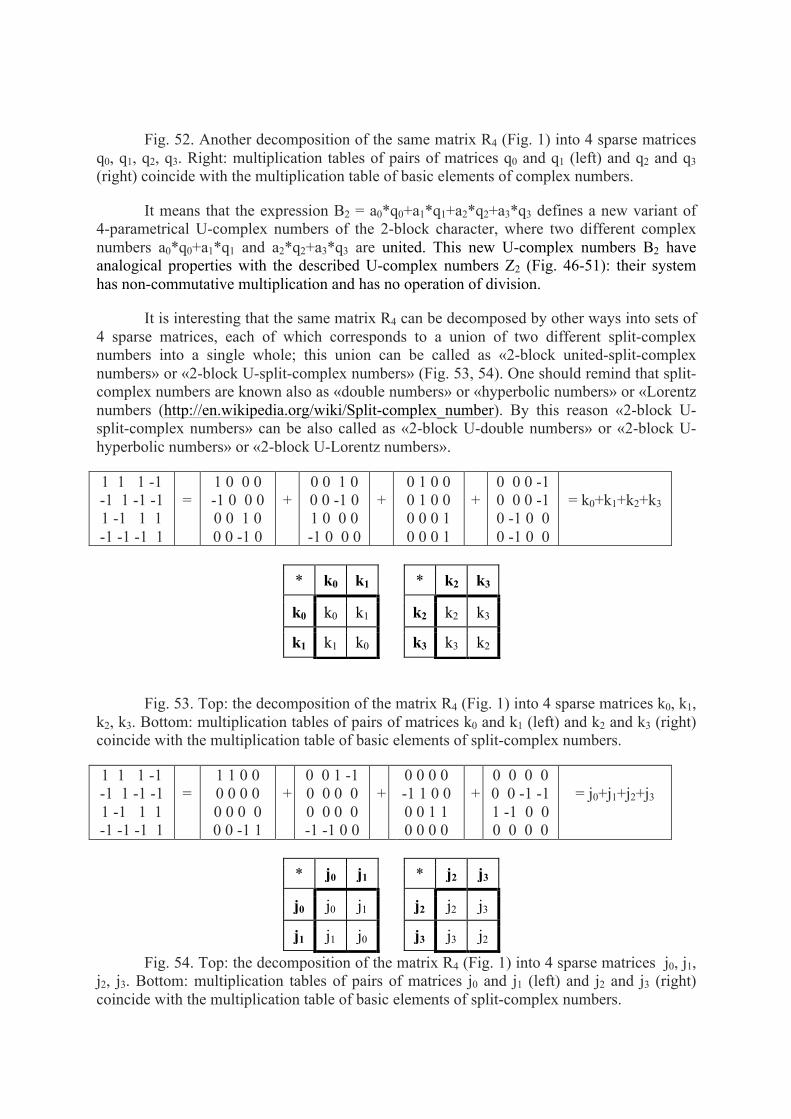
Fig. 52. Another decomposition of the same matrix R4 (Fig. 1) into 4 sparse matrices q0, q1, q2, q3. Right: multiplication tables of pairs of matrices q0 and q1 (left) and q2 and q3 (right) coincide with the multiplication table of basic elements of complex numbers.

It means that the expression B2 = a0*q0+a1*q1+a2*q2+a3*q3 defines a new variant of 4-parametrical U-complex numbers of the 2-block character, where two different complex numbers a0*q0+a1*q1 and a2*q2+a3*q3 are united. This new U-complex numbers B2 have analogical properties with the described U-complex numbers Z2 (Fig. 46-51): their system has non-commutative multiplication and has no operation of division.

It is interesting that the same matrix R4 can be decomposed by other ways into sets of 4 sparse matrices, each of which corresponds to a union of two different split-complex numbers into a single whole; this union can be called as «2-block united-split-complex numbers» or «2-block U-split-complex numbers» (Fig. 53, 54). One should remind that split-complex numbers are known also as «double numbers» or «hyperbolic numbers» or «Lorentz numbers (http://en.wikipedia.org/wiki/Split-complex_number). By this reason «2-block U-split-complex numbers» can be also called as «2-block U-double numbers» or «2-block U-hyperbolic numbers» or «2-block U-Lorentz numbers».

1 1 1 -1 -1 1 -1 -1 1 -1 1 1 -1 -1 -1 1

=

1 0 0 0 -1 0 0 0 0 0 1 0 0 0 -1 0

+

0 0 1 0 0 0 -1 0 1 0 0 0 -1 0 0 0

+

0 1 0 0 0 1 0 0 0 0 0 1 0 0 0 1

+

0 0 0 -1 0 0 0 -1 0 -1 0 0 0 -1 0 0

= k0+k1+k2+k3

* k0 k1

k0 k0 k1

k1 k1 k0

* k2 k3

k2 k2 k3

k3 k3 k2

Fig. 53. Top: the decomposition of the matrix R4 (Fig. 1) into 4 sparse matrices k0, k1, k2, k3. Bottom: multiplication tables of pairs of matrices k0 and k1 (left) and k2 and k3 (right) coincide with the multiplication table of basic elements of split-complex numbers.

1 1 1 -1 -1 1 -1 -1 1 -1 1 1 -1 -1 -1 1

=

1 1 0 0 0 0 0 0 0 0 0 0 0 0 -1 1

+

0 0 1 -1 0 0 0 0 0 0 0 0 -1 -1 0 0

+

0 0 0 0 -1 1 0 0 0 0 1 1 0 0 0 0

+

0 0 0 0 0 0 -1 -1 1 -1 0 0 0 0 0 0

= j0+j1+j2+j3

* j0 j1

j0 j0 j1

j1 j1 j0

* j2 j3

j2 j2 j3

j3 j3 j2

Fig. 54. Top: the decomposition of the matrix R4 (Fig. 1) into 4 sparse matrices j0, j1, j2, j3. Bottom: multiplication tables of pairs of matrices j0 and j1 (left) and j2 and j3 (right) coincide with the multiplication table of basic elements of split-complex numbers.

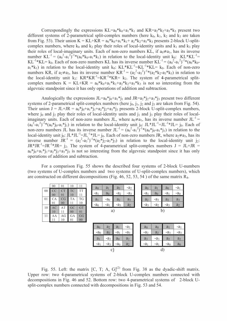
Correspondingly the expressions KL=a0*k0+a1*k1 and KR=a2*k2+a3*k3 present two different systems of 2-parametrical split-complex numbers (here k0, k1, k2 and k3 are taken from Fig. 53). Their union K = KL+KR = a0*k0+a1*k1+ a2*k2+a3*k3 presents 2-block U-split-complex numbers, where k0 and k2 play their roles of local-identity units and k1 and k3 play their roles of local-imaginary units. Each of non-zero numbers KL, if a0≠a1, has its inverse number KL-1 = (a0

2-a12)-1*(a0*k0-a1*k1) in relation to the local-identity unit k0: KL*KL-1=

KL-1*KL= k0. Each of non-zero numbers KL has its inverse number KL-1 = (a02-a1

2)-1*(a0*k0-a1*k1) in relation to the local-identity unit k0: KL*KL-1=KL-1*KL= k0. Each of non-zero numbers KR, if a2≠a3, has its inverse number KR-1 = (a2

2-a32)-1*(a2*k2-a3*k3) in relation to

the local-identity unit k2: KR*KR-1=KR-1*KR= k2. The system of 4-parametrical split-complex numbers K = KL+KR = a0*k0+a1*k1+a2*k2+a3*k3 is not so interesting from the algevraic standpoint since it has only operations of addition and subtraction.

Analogically the expressions JL=a0*j0+a1*j1 and JR=a2*j2+a3*j3 present two different systems of 2-parametrical split-complex numbers (here j0, j1, j2 and j3 are taken from Fig. 54). Their union J = JL+JR = a0*j0+a1*j1+a2*j2+a3*j3 presents 2-block U-split-complex numbers, where j0 and j2 play their roles of local-identity units and j1 and j3 play their roles of local-imaginary units. Each of non-zero numbers JL, where a0≠a1, has its inverse number JL-1 = (a0

2-a12)-1*(a0*j0-a1*j1) in relation to the local-identity unit j0: JL*JL-1=JL-1*JL= j0. Each of

non-zero numbers JL has its inverse number JL-1 = (a02-a1

2)-1*(a0*j0-a1*j1) in relation to the local-identity unit j0: JL*JL-1=JL-1*JL= j0. Each of non-zero numbers JR, where a2≠a3, has its inverse number JR-1 = (a2

2-a32)-1*(a2*j2-a3*j3) in relation to the local-identity unit j2:

JR*JR-1=JR-1*JR= j2. The system of 4-parametrical split-complex numbers J = JL+JR = a0*j0+a1*j1+a2*j2+a3*j3 is not so interesting from the algevraic standpoint since it has only operations of addition and subtraction.

For a comparison Fig. 55 shows the described four systems of 2-block U-numbers (two systems of U-complex numbers and two systems of U-split-complex numbers), which are constructed on different decompositions (Fig. 46, 52, 53, 54 ) of the same matrix R4.

00 01 10 11 00 CC

00 CT 01

TC 10

TT 11

01 CA 01

CG 00

TA 11

TG 10

10 AC 10

AT 11

GC 00

GT 01

11 AA 11

AG 10

GA 01

GG 00

a0 a1 a3 -a2 -a1 a0 -a2 -a3 a1 -a0 a2 a3

-a0 -a1 -a3 a2 a)

a0 a1 a0 -a1 -a1 a0 -a1 -a0 a2 -a3 a2 a3 -a3 -a2 -a3 a2

b)

a0 a2 a1 -a3

-a0 a2 -a1 -a3 a1 -a3 a0 a2 -a1 -a3 -a0 a2

c)

a0 a0 a1 -a1 -a2 a2 -a3 -a3 a3 -a3 a2 a2 -a1 -a1 -a0 a0

d)

Fig. 55. Left: the matrix [C, T; A, G](2) from Fig. 38 as the dyadic-shift matrix. Upper row: two 4-parametrical systems of 2-block U-complex numbers connected with decompositions in Fig. 46 and 52. Bottom row: two 4-parametrical systems of 2-block U-split-complex numbers connected with decompositions in Fig. 53 and 54.

One can see from Fig. 55 that all these 4 systems of 2-block U-numbers have the identical mosaic of locations of signs + and – (marked by black and white colors). They differ only by the distribution of parameters a0, a1, a2, a3, which reflects structures of basic elements of corresponding 2-block U-numbers «a», «b», «c» and «d» in Fig. 55. This structures are not chaotic but they are regular from the standpoint of the representation of genetic matrices [C, T; A, G](n) as the dyadic-shift matrix (the notion of dyadic-shift matrices is used in discrete signals processing and noise-immunity coding [Ahmed, Rao, 1975]). This representation has been described in our works [Petoukhov, 2008b, 2011a; Petoukhov, He, 2010] on the basis of 3 pairs of binary-oppositional traits of nitrogenous bases of DNA and RNA. Fig. 55,left shows the representation of genetic matrices [C, T; A, G](2) as the dyadic-shift matrix, where each of cells has its binary numeration. For example, in the matrix «a», which correspond to the set of basic matrices e0, e1, e2, e3 in Fig. 46, non-zero entries of the matrices e0, e1, e2, e3 are located in cells with the following binary numerations in the dyadic-shift matrix:

-‐ for e0 - in cells 00, 00, 11, 11 (the parameter a0 is located in these cells); -‐ for e1 - in cells 01, 01, 10, 10 (the parameter a1 is located in these cells); -‐ for e2 - in cells 00, 00, 11, 11 (the parameter a2 is located in these cells); -‐ for e3 – in cells 01, 01, 10, 10 (the parameter a3 is located in these cells).

Here the matrices e0 and e2, which are local-real units in U-numbers “a”, have the identical set of binary numerations 00, 00, 11, 11 for their non-zero entries; but non-zero entries of the matrix e0 correspond to doublets with the first letter C and A in contrast to non-zero entries of the marix e2, which correspond to doublets with the first letter G and T. The matrices e1 and e3, which are local-imaginary units in U-numbers “a”, also have the identical set of binary numerations 01, 01, 10, 10 for their non-zero entries; but non-zero entries of the matrix e1 correspond to doublets with the first letter C and A in contrast to non-zero entries of the marix e3, which correspond to doublets with the first letter G and T.

The similar situation is realized for the systems of U-numbers «b», «c» and «d» in Fig. 55 and also for 4-block U-complex numbers, which are based on appropriate decompositions of the matrix R8 (Fig. 1).

As known the set of 16 doubles is divided into 2 equal subsets of 8 strong doublets and 8 weak doublets (Fig. 36). The connection of the genetic alphabets of DNA and RNA with the described systems of 4-parametrical U-numbers (the systems «a», «b», «c» and «d» in Fig. 55) allows to suppose the following: the set of 16 doublets can be divided by nature into other separate subsets of equivalency, where 4 subsets exist with 4 doublets in each on the basis of appropriate traits of equivalency connected with the dyadic-shift matrices and with binary-oppositional traits of nitrogenous bases. For example, in the case of U-complex numbers represented by the matrix «a» in Fig. 55, the following division can be supposed:

- the subset for non-zero entries of the basic matrix e0 includes doublets CC, CG, AT, AA;

- the subset for non-zero entries of the basic matrix e1 includes doublets CT, CA, AC, AG;

- the subset for non-zero entries of the basic matrix e2 includes doublets TT, TA, GC, GG;

- the subset for non-zero entries of the basic matrix e3 includes doublets TC, TG, GT, GA.

For systems of U-numbers represented by matrices «b», «c» and «d» (Fig. 55), other

approprite combinations of doublets exist to provide their 4 sets with 4 doublets in each on the basis of relevant traits of equivalency. It was described in publications [Petoukhov, 2008b, 2011a, 2012b; Petoukhov, He, 2009] that each of 16 doublets and each of 64 triplets has its own binary numeration on the basis of 3 kinds of objective binary-oppositional traits of nitrogenous bases of DNA and RNA in connection with dyadic groups of binary numbers, the tensor family of genetic matrices [C, A; T, G](n) and with binary numeration in dyadic-shift matrices. It gives an opportunity for genetic system to mark each of cases of 4 subsets of doublets in matrices «a», «b», «c» and «d» (Fig. 55) by means of its individual token. Using appropriate systems of such tokens, bioinformational system of living organism can parallely apply different kinds of U-hypercomplex numbers in providing multi-channel communication among its different physiological parts and also communication with the external world. From the standpoint of such approach, a living organism has no a single kind of numeric system but many different kinds of systems U-hypercomplex numbers (an organism is a poly-linguistic object). The author believes that many secrets of genetic systems and genetic phenomena are connected with such multi-linguistics of genetic systems.

Let us turn now to the matrix R8, which is the Walsh-representation of the genetic matrix [C, T; A, G](3). We show here only two of several examples of its possible decompositions (Fig. 56 and 57), which lead to 4-block U-complex numbers and 4-block U-split-complex numbers.

R8 =

1 0 0 0 0 0 0 0 1 0 0 0 0 0 0 0 0 0 1 0 0 0 0 0 0 0 1 0 0 0 0 0 0 0 -1 0 0 0 0 0 0 0 -1 0 0 0 0 0 -1 0 0 0 0 0 0 0 -1 0 0 0 0 0 0 0

+

0 0 1 0 0 0 0 0 0 0 1 0 0 0 0 0 -1 0 0 0 0 0 0 0 -1 0 0 0 0 0 0 0 1 0 0 0 0 0 0 0 1 0 0 0 0 0 0 0 0 0 -1 0 0 0 0 0 0 0 -1 0 0 0 0 0

+

0 1 0 0 0 0 0 0 0 1 0 0 0 0 0 0 0 0 0 1 0 0 0 0 0 0 0 1 0 0 0 0 0 0 0 -1 0 0 0 0 0 0 0 -1 0 0 0 0 0 -1 0 0 0 0 0 0 0 -1 0 0 0 0 0 0

+

0 0 0 1 0 0 0 0 0 0 0 1 0 0 0 0 0 -1 0 0 0 0 0 0 0 -1 0 0 0 0 0 0 0 1 0 0 0 0 0 0 0 1 0 0 0 0 0 0 0 0 0 -1 0 0 0 0 0 0 0 -1 0 0 0 0

+

0 0 0 0 0 0 -1 0 0 0 0 0 0 0 -1 0 0 0 0 0 -1 0 0 0 0 0 0 0 -1 0 0 0 0 0 0 0 1 0 0 0 0 0 0 0 1 0 0 0 0 0 0 0 0 0 1 0 0 0 0 0 0 0 1 0

+

0 0 0 0 1 0 0 0 0 0 0 0 1 0 0 0 0 0 0 0 0 0 -1 0 0 0 0 0 0 0 -1 0 0 0 0 0 0 0 1 0 0 0 0 0 0 0 1 0 0 0 0 0 -1 0 0 0 0 0 0 0 -1 0 0 0

+

0 0 0 0 0 0 0 -1 0 0 0 0 0 0 0 -1 0 0 0 0 0 -1 0 0 0 0 0 0 0 -1 0 0 0 0 0 0 0 1 0 0 0 0 0 0 0 1 0 0 0 0 0 0 0 0 0 1 0 0 0 0 0 0 0 1

+

0 0 0 0 0 1 0 0 0 0 0 0 0 1 0 0 0 0 0 0 0 0 0 -1 0 0 0 0 0 0 0 -1 0 0 0 0 0 0 0 1 0 0 0 0 0 0 0 1 0 0 0 0 0 -1 0 0 0 0 0 0 0 -1 0 0

* v0 v1

v0 v0 v1

v1 v1 -v0

* v2 v3

v2 v2 v3

v3 v3 -v2

* v4 v5

v4 v4 v5

v5 v5 -v4

* v6 v7

v6 v6 v7

v7 v7 -v6

Fig. 56. The decomposition of the matrix R8 (Fig. 1) into the set of 8 sparse matrices:

R8=v0+v1+v2+v3+v4+v5+v6+v7. Each of the following pairs of these 8 matrices (v0 and v2; v2 and v3; v4 and v5; v6 and v7) forms a set, which is closed under multiplication. These sets define multiplication tables, which coincide with the multiplication table of the system of complex numbers (the lower row).

Each of the following expressions means a separate system of complex numbers represented in the form of (8*8)-matrices: a0*v0+a1*v1, a2*v2+a3*v3, a4*v4+a5*v5, a6*v6+a7*v7. Their sum V = a0*v0+a1*v1, a2*v2+a3*v3, a4*v4+a5*v5, a6*v6+a7*v7 represents the system of 4-block U-complex numbers.

Fig. 57 shows another decomposition of the same matrix R8 into 8 sparse matrices: R8 = p0+p1+p2+p3+p4+p5+p6+p7:

R8 =

1 0 0 0 0 0 0 0 0 1 0 0 0 0 0 0 -‐1 0 0 0 0 0 0 0 0 -‐1 0 0 0 0 0 0 1 0 0 0 0 0 0 0 0 1 0 0 0 0 0 0 -‐1 0 0 0 0 0 0 0 0 -‐1 0 0 0 0 0 0

+

0 1 0 0 0 0 0 0 1 0 0 0 0 0 0 0 0 -‐1 0 0 0 0 0 0 -‐1 0 0 0 0 0 0 0 0 1 0 0 0 0 0 0 1 0 0 0 0 0 0 0 0 -‐1 0 0 0 0 0 0 -‐1 0 0 0 0 0 0 0

+

0 0 1 0 0 0 0 0 0 0 0 1 0 0 0 0 0 0 1 0 0 0 0 0 0 0 0 1 0 0 0 0 0 0 -‐1 0 0 0 0 0 0 0 0 -‐1 0 0 0 0 0 0 -‐1 0 0 0 0 0 0 0 0 -‐1 0 0 0 0

+

0 0 0 1 0 0 0 0 0 0 1 0 0 0 0 0 0 0 0 1 0 0 0 0 0 0 1 0 0 0 0 0 0 0 0 -‐1 0 0 0 0 0 0 -‐1 0 0 0 0 0 0 0 0 -‐1 0 0 0 0 0 0 -‐1 0 0 0 0 0

+

0 0 0 0 1 0 0 0 0 0 0 0 0 1 0 0 0 0 0 0 -‐1 0 0 0 0 0 0 0 0 -‐1 0 0 0 0 0 0 1 0 0 0 0 0 0 0 0 1 0 0 0 0 0 0 -‐1 0 0 0 0 0 0 0 0 -‐1 0 0

+

0 0 0 0 0 1 0 0 0 0 0 0 1 0 0 0 0 0 0 0 0 -‐1 0 0 0 0 0 0 -‐1 0 0 0 0 0 0 0 0 1 0 0 0 0 0 0 1 0 0 0 0 0 0 0 0 -‐1 0 0 0 0 0 0 -‐1 0 0 0

+

0 0 0 0 0 0 -‐1 0 0 0 0 0 0 0 0 -‐1 0 0 0 0 0 0 -‐1 0 0 0 0 0 0 0 0 -‐1 0 0 0 0 0 0 1 0 0 0 0 0 0 0 0 1 0 0 0 0 0 0 1 0 0 0 0 0 0 0 0 1

+

0 0 0 0 0 0 0 -‐1 0 0 0 0 0 0 -‐1 0 0 0 0 0 0 0 0 -‐1 0 0 0 0 0 0 -‐1 0 0 0 0 0 0 0 0 1 0 0 0 0 0 0 1 0 0 0 0 0 0 0 0 1 0 0 0 0 0 0 1 0

* p0 p1

p0 p0 p1

p1 p1 p0

* p2 p3

p2 p2 p3

p3 p3 p2

* p4 p5

p4 p4 p5

p5 p5 p4

* p6 p7

p6 p6 p7

p7 p7 p6

Fig. 57. The decomposition of the matrix R8 (Fig. 1) into the set of 8 sparse matrices: R8=p0+p1+p2+p3+p4+p5+p6+p7. Each of the following pairs of these 8 matrices (v0 and v2; v2 and v3; v4 and v5; v6 and v7) forms a set, which is closed under multiplication. These sets define multiplication tables, which coincide with the multiplication table of the system of split-complex numbers (the lower row).

Each of the following expressions means a separate system of split-complex numbers represented in the form of (8*8)-matrices: a0*p0+a1*p1, a2*p2+a3*p3, a4*p4+a5*p5, a6*p6+a7*p7. Their sum P = a0*p0+a1*p1+a2*p2+a3*p3+a4*p4+a5*p5 +a6*p6+a7*p7 represents the system of 4-block U-split-complex numbers.

Decompositions of the matrix R8 can lead not only to systems of U-numbers with 2-parametrical blocks but also to systems of U-numbers with 4 parametrical blocks as the following example shows (Fig. 58).

R8 =

1 0 0 0 0 0 0 0 1 0 0 0 0 0 0 0 0 0 1 0 0 0 0 0 0 0 1 0 0 0 0 0 0 0 0 0 1 0 0 0 0 0 0 0 1 0 0 0 0 0 0 0 0 0 1 0 0 0 0 0 0 0 1 0

+

0 0 1 0 0 0 0 0 0 0 1 0 0 0 0 0 -1 0 0 0 0 0 0 0 -1 0 0 0 0 0 0 0 0 0 0 0 0 0 1 0 0 0 0 0 0 0 1 0 0 0 0 0 -1 0 0 0 0 0 0 0 -1 0 0 0

+

0 0 0 0 1 0 0 0 0 0 0 0 1 0 0 0 0 0 0 0 0 0 -1 0 0 0 0 0 0 0 -1 0 1 0 0 0 0 0 0 0 1 0 0 0 0 0 0 0 0 0 -1 0 0 0 0 0 0 0 -1 0 0 0 0 0

+

0 0 0 0 0 0 -1 0 0 0 0 0 0 0 -1 0 0 0 0 0 -1 0 0 0 0 0 0 0 -1 0 0 0 0 0 -1 0 0 0 0 0 0 0 -1 0 0 0 0 0 -1 0 0 0 0 0 0 0 -1 0 0 0 0 0 0 0

+

0 1 0 0 0 0 0 0 0 1 0 0 0 0 0 0 0 0 0 1 0 0 0 0 0 0 0 1 0 0 0 0 0 0 0 0 0 1 0 0 0 0 0 0 0 1 0 0 0 0 0 0 0 0 0 1 0 0 0 0 0 0 0 1

+

0 0 0 1 0 0 0 0 0 0 0 1 0 0 0 0 0 -‐1 0 0 0 0 0 0 0 -‐1 0 0 0 0 0 0 0 0 0 0 0 0 0 1 0 0 0 0 0 0 0 1 0 0 0 0 0 -‐1 0 0 0 0 0 0 0 -‐1 0 0

+

0 0 0 0 0 1 0 0 0 0 0 0 0 1 0 0 0 0 0 0 0 0 0 -‐1 0 0 0 0 0 0 0 -‐1 0 1 0 0 0 0 0 0 0 1 0 0 0 0 0 0 0 0 0 -‐1 0 0 0 0 0 0 0 -‐1 0 0 0 0

+

0 0 0 0 0 0 0 -‐1 0 0 0 0 0 0 0 -‐1 0 0 0 0 0 -‐1 0 0 0 0 0 0 0 -‐1 0 0 0 0 0 -‐1 0 0 0 0 0 0 0 -‐1 0 0 0 0 0 -‐1 0 0 0 0 0 0 0 -‐1 0 0 0 0 0 0

* w0 w1 w2 w3

w0 w0 w1 w2 w3

w1 w1 -w0 w3 -w2

w2 w2 -w3 w0 -w1

w3 w3 w2 w1 w0

* w4 w5 w6 w7

w4 w4 w5 w6 w7

w5 w5 -w4 w7 -w6

w6 w6 -w7 w4 -w5

w7 w7 w6 w5 w4

Fig. 58. The decomposition of the matrix R8 (Fig. 1) into the set of 8 sparse matrices: R8=w0+w1+w2+w3+w4+w5+w6+w7. Each of the following Each of the following quadruples of matrices (w0, w1, w2 and w3; w4, w5, w6 and w7) forms a set, which is closed under multiplication. These sets define multiplication tables, which coincide with the multiplication table of the 4-parametrical system of split-quaternions of J.Cockle (https://en.wikipedia.org/wiki/Split-quaternion).

Each of the following expressions means a separate system of split-quaternions represented in the form of (8*8)-matrices: a0*w0+a1*w1+a2*w2+a3*w3 and a4*w4+a5*w5+a6*w6+a7*w7. Their sum W = a0*w0+a1*w1+a2*w2+a3*w3+a4*w4+a5*w5 +a6*w6+a7*w7 represents the system of 2-block U-split-quaternions. The system of 2-block U-split-quaternions has operations of addition, subtraction and non-commutative multiplication.

16. TENSOR FAMILIES OF DIAGONAL UNITED-HYPERCOMPLEX NUMBERS

The following important question arises: whether such systems of U-complex numbers exist, which possess operations of commutative multiplication and division? Below we give positive answer on this question and show systems with these operations and addiionally with divisors of zero. These systems are connected with the genetic matrices and their Walsh-representations R4 and R8 (Fig. 1). In the matrix R4 (Fig. 1) the mosaic of two quadrants along the main diagonal is mirror-antisymmetric to the mosaic of two quadrants along the second diagonal in relation to the middle horizontal line. The operation of the mirror-antisymmetric transformation is given by the matrix J in the expression (12), the square of which J2 is equal to the identical (4*4)-matrix: J = [0,0,0,-1; 0,0,-1,0; 0,-1,0,0; -1, 0,0,0], J2 = [1,0,0,0; 0,1,0,0; 0,0,1,0; 0,0,0,1] (12) Fig. 59 illustrates that the matrix R4 is the sum of 2 sparse matrices R40 and R41 of diagonal types, non-zero parts of which coincide with two quadrants along the main diagonal and along the second diagonal correspondingly.

R4 = R40+R41 =

1 1 1 -1 -1 1 -1 -1 1 -1 1 1 -1 -1 -1 1

=

1 1 0 0 -1 1 0 0 0 0 1 1 0 0 -1 1

+

0 0 1 -1 0 0 -1 -1 1 -1 0 0 -1 -1 0 0

Fig. 59. The matrix R4 is the sum of two matrices R40 and R41.

The mirror-antisymmetric transformation J from the expression (12) transforms the

matrix R41 into the matrix R40. Taking this into account, the initial matrix R4 = R40+R41 = R40 + J*R40 = R40*(E+J), where E is the identity (4*4)-matrix and E+J is the split-complex number with unit coordinates since the set of matrices E and J is closed under multiplication and its multiplication table coincides with the muliplication table of split-complex numbers (the mirror-antisymmetric transformation J represents the imaginary unit in this set). In other word, the matrix R4 is the product of the matrix R40 with this split-complex number. Correspondingly a special attention should be devoted to the sparse matrix R40 of the diagonal type, non-zero parts of which represents numeric mosaic of the quadrants along the main diagonal in the genetic matrix R4.

Fig.60 shows a decomposition of this matrix R40 = d0+d1+d2+d3, from the standpoint of which R40 is diagonal 2-block U-complex number with unit coordinates.

R40 =

1 1 0 0 -1 1 0 0 0 0 1 1 0 0 -1 1

=

1 0 0 0 0 1 0 0 0 0 0 0 0 0 0 0

+

0 1 0 0 -1 0 0 0 0 0 0 0 0 0 0 0

+

0 0 0 0 0 0 0 0 0 0 1 0 0 0 0 1

+

0 0 0 0 0 0 0 0 0 0 0 1 0 0 -1 0

= d0+d1+ d2+d3

* d0 d1

d0 d0 d1

d1 d1 -d0

* d2 d3

d2 d2 d3

d3 d3 -d2

Fig. 59a. Top: the decomposition of the block-diagonal matrix R40 into 4 sparse matrices d0, d1, d2, d3. Bottom: multiplication tables for the pair d0 and d2 and for the pair d2 and d3 coincide with the multiplication table of complex numbers.

The pair of matrices d0 and d1 forms the set, which is closed under multiplication and which defines the multiplication table of complex numbers (Fig. 59a, bottom). The same is true for the pair of matrices d2 and d3. It means that the matrix R40 is the 2-block united-complex number of the diagonal type with unit coordinates. These basis elements d0, d1, d2, d3 of two systems of complex numbers define the following general view of these complex numbers SL and SR: SL = a0*d0+a1*d1 and SR = a2*d2+a3*d3. Fig. 60 shows the corresponding general view of the system of 2-block diagonal U-complex numbers S = a0*d0+a1*d1+a2*d2+a3*d3 having 4 parameters (a0, a1, a2, a3). One should mention that the whole set of matrices d0, d1, d2, d3 is not closed under multiplication and it does not represent any of hypercomplex numbers.

SL = a0*d0+a1*d1 = [a0, a1, 0, 0 -a1, a0, 0, 0 0, 0, 0, 0 0, 0, 0, 0]

SR = a2*d2+a3*d3 = [0, 0, 0, 0 0, 0, 0, 0 0, 0, a2, a3 0, 0, -a3, a2]

S = SL+SR = a0*d0+a1*d1 +a2*d2+a3*d3 = [a0, a1, 0, 0 -a1, a0, 0, 0 0, 0, a2, a3 0, 0, -a3, a2]

SL-1 = (a02 + a1

2)-1 * (a0*d0-a1*d1); SL*SL-1=SL-1*SL=d0, where d0 – the local-identity matrix for SL.

SR-1 = (a22 + a3

2)-1* (a2*d2-a3*d3);

SR*SR-1=SR-1*SR=d2 where d2 – the local-identity matrix for SR.

S-1 = (a02+a1

2)-1*(a0*d0-a1*d1) + (a2

2+a32)-1*(a2*d2-a3*d3) = SL-1 + SR-1.

S*S-1 = S-1*S = E, where E = [1,0,0,0; 0,1,0,0; 0,0,1,0; 0,0,0,1] – the identity matrix

Fig. 60. Upper row: diagonal U-complex numbers S of 2-block type, which unite complex numbers SL and SR. Lower row: expressions for inverse matrices SL-1, SR-1 and S-1.

The classical identity matrix E=[1 0 0 0; 0 1 0 0; 0 0 1 0; 0 0 0 1] is absent in the set of matrices SL and SR, where - beside this - each matrix has zero determinant (Fig. 60). Consequently the notion of the inverse matrix SL-1 or SR-1 (as SL*SL-1=E or SR*SR-1 =E) can’t be defined in relation to the identity matrix E in accordance with the famous theorem about inverse matrices for matrices with zero determinant in the case of the complete set of matrices [Bellman, 1960, Chapter 6, § 4]. But we analyze not the complete set of (4*4)-matrices but very limited special sets of matrices SL and SR. The system SL has the matrix d0 (Fig. 59), which possesses all properties of its identity matrix for any matrix SL since d0*SL = SL*d0 = SL and d0

2 = d0. In the frame of the system of matrices SL, where locally the matrix d0 plays the role of the identity matrix (the local-identity matrix), one can define - for any non-zero matrix SL - the inverse matrix SL-1 in relation to the matrix d0 on the basis of equations: SL*SL-1 = SL-1*SL = d0. One can check that such inverse matrix is defined by the following expression: SL-1 = (a0

2 + a12)-1*(a0*d0-a1*d1) (Fig. 60).

By analogy, the system of matrices SR has the matrix d2 (Fig. 59a), which possesses all properties of the identity matrix for any matrix SR since d2*SR = SR*d2 = SR and d2

2 = d2. In the frame of the system of matrices SR, where the matrix d2 plays locally the role of the identity matrix (the local-identity matrix), one can define - for any non-zero matrix SR - the inverse matrix SR-1 in relation to the matrix d2 on the base of equations: SR*SR-1 = SR-1*SR = d2 .

Any of nonzero 2-block diagonal U-complex numbers S = SL+SR = a0*d0+a1*d1 +a2*d2+a3*d3 has its inverse number S-1 of the same type in relation to the ordinary identity (4*4)-matrix E=[1,0,0,0; 0,1,0,0; 0,0,1,0; 0,0,0,1]: S*S-1 = S-1*S=E, where S-1 = (a0

2+a12)-1*

(a0*d0-a1*d1) + (a22+a3

2)-1*(a2*d2-a3*d3) = SL-1 + SR-1. In other words, in this system the inverse U-number S-1 is equal to the sum of inverse numbers SL-1 and SR-1.

Fig. 61 shows that the multiplication between any two members of the system of 2-block diagonal U-complex numbers is commutative and it gives a new member on the same system. (a0*d0+a1*d1+a2*d2+a3*d3)*(b0*d0+b1*d1+b2*d2+b3*d3) = (b0*d0+b1*d1+b2*d2+b3*d3)*(a0*d0+a1*d1+a2*d2+a3*d3) = (c0*d0+c1*d1+c2*d2+c3*d3), where c0 = a0*b0-a1*b1, c1 = a0*b1+a1*b0, c2= a2*b2-a3*b3, c3 = a2*b3+a3*b2.

Fig. 61. Commutative multiplication of two members of the system of 2-block diagonal U-complex numbers from Fig. 60.

The system of 2-block diagonal U-complex numbers S has operations of addition, subtraction, commutative multiplication and division (division is defined by multiplication with the inverse diagonal U-numbers S-1, which is equal to the sum of inverse complex numbers SL-1 and SR-1). This system has zero divisors; it means that the system has non-zero matrices, the product of which gives zero. Indeed, the product of non-zero matrices SL and SR is equal to zero matrix: SL*SR=SR*SL=0. (If split-complex numbers are used in both diagonal blocks of the matrix S in Fig. 60 instead of complex numbers, the system of diagonal 2-block U-split-complex numbers arises, which also possesses operations of addition, subtraction, commutative multiplication and division and which has divisors of zero).

Now let us consider questions about norms and the scalar product in this system of 2-block diagonal U-complex numbers. As known a conjugate number Z for complex number Z=a+b*i is defined by inversion of sign of its imaginary part: Z = a-b*i. The norm |Z| of complex number Z is defined by the expression |Z| = Z*Z = a2+b2.

Correspondingly, conjugate numbers SL and SR for complex numbers SL = a0*d0+a1*d1 and SR = a2*d2+a3*d3 are created by inversion of sign in their local-imaginary parts: SL = a0*d0-a1*d1 and SR = a2*d2-a3*d3. In this case the norm |SL| of complex numbers SL is equal to: |SL| = SL*SL = (a0

2+a12)*d0. The norm |SR| of complex numbers SR is equal

to: |SR| = SR*SR = (a22+a3

2)*d2. By definition, the conjugate number S for any of DU-complex numbers S = SL+SR =

a0*d0+a1*d1+a2*d2+a3*d3 is also created by means of inversion of signs of its local-imaginary parts a1*d1 and a3*d3: S = a0*d0-a1*d1+a2*d2-a3*d3. The norm |S| is defined by the expression |S| = S* S = (a0*d0+a1*d1+a2*d2+a3*d3) * (a0*d0-a1*d1+a2*d2-a3*d3) = (a0

2+a12)*d0 +

(a22+a3

2)*d2 = |SL|+|SR|. In other words,the norm |S| of any of these diagonal U-complex numbers is equal to the sum of norms |SL| and |SR| in its two separate blocks of complex numbers.

As known, the scalar product <Z1,Z2> for two vectors of the complex plane Z1 = a0+a1*i and Z2 = b0+b1*i, which are usually represented by (2*2)-matrices [a0, a1; -a1, a0] and [b0, b1; -b1, b0], is defined by means the expression <Z1,Z2> = Z1*Z2 = (a0+a1*i )*( b0-b1*i) = (a0*b0+a1*b1)+(a1*b0-a0*b1)*i. By analogy one can define the scalar product <SL1,SL2> for two vectors SL1 = a0*d0+a1*d1 and SL2 = b0*d0+b1*d1 from the set of (4*4)-matrices SL (Fig. 60) by means of the similar expression: <SL1,SL2> = SL1*SL2 = (a0*d0+a1*d1) * (b0*d0-b1*d1) = (a0*b0+a1*b1)*d0 + (a1*b0-a0*b1)*d1. So the result of scalar product

<SL1,SL2> coincides with the scalar product <Z1,Z2> but - instead of the real unit “1” and the imaginary unit “i” in <Z1,Z2> - the expression <SL1,SL2> uses the local-real unit d0 and the local-imaginary unit d1. Analogically the scalar product <SR1,SR2> for two vectors SR1 = a2*d2+a3*d3 and SR2 = b2*d2+b3*d3 from the set of (4*4)-matrices SR (Fig. 60) can be defined by means of the expression <SR1,SR2> = SR1*SR2 = (a2*d2+a3*d3)*(b2*d2-b3*d3) = (a2*b2+a3*b3)*d2 + (a3*b2-a2*b3)*d3, where the local-real unit d2 and the local-imaginary unit d3 are used.

The scalar product <S1,S2> of two 2-block diagonal U-complex numbers S1=SL1+SR1=a0*d0+a1*d1+a2*d2+a3*d3 and S2= SL2+SR2= b0*d0+b1*d1+b2*d2+b3*d3 is defined by the analogical expression: <S1,S2> = S1*S2 = (a0*d0+a1*d1+a2*d2+a3*d3) * (b0*d0-b1*d1+b2*d2-b3*d3) = (a0*b0+a1*b1)*d0 + (a1*b0-a0*b1)*d1 + (a2*b2+a3*b3)*d2 + (a3*b2-a2*b3)*d3 = <SL1,SL2> + <SR1,SR2>. In other words, the scalar product of two 2-block diagonal U-complex numbers S1 and S2 is equal to the sum of scalar products of their corresponding blocks of complex numbers.

[x0,x1,x2,x3] * SL = [ a0*x0-a1*x1, a0*x1+a1*x0, 0, 0 ] SL * [x0,x1,x2,x3].' = [a0*x0+a1*x1; a0*x1-a1*x0; 0; 0 ] [x0,x1,x2,x3] * SR = [ 0, 0, a2*x2-a3*x3, a2*x3+a3*x2] SR * [x0,x1,x2,x3].' = [ 0; 0; a2*x2+a3*x3; a2*x3-a3*x2 ]

Fig. 62. Multiplication of matrix operators SL and SR (Fig. 54) with a vector X=[x0,x1,x2,x3] from the right side and from the left side leads to a possibility of a selective manage of subspaces.

Fig. 62 shows results of actions of the matrix operators SL and SR on a 4-dimensional vector X=[x0,x1,x2,x3] from the right side and from the left side. In both cases the action of matrix operators SL leads to a possibility of a selective manage of vectors of 2-dimensional subspaces inside configurational 4-dimensional spaces [x0,x1,x2,x3]: the resulting non-zero vectors exist only in the subspace (x0,x1), where they can be managed arbitrary by means of parameters a0 and a1 of the operator SL. If the parameters a0 and a1 are functions of time, then vectors [x0,x1,x2,x3]*SL and SL*[x0,x1,x2,x3] move along corresponding trajectories only in the plane (x0,x1).

The action of matrix operators SR in both cases also leads to a possibility of a selective manage of vectors of 2-dimensional subspaces inside configurational 4-dimensional spaces [x0,x1,x2,x3]. In this case the resulting non-zero vectors exist only in another subspace (x2,x3), where they can be managed by means of parameters a2 and a3 of the operator SR. If the parameters a2 and a3 are functions of time, then vectors [x0,x1,x2,x3]*SR and SR*[x0,x1,x2,x3] move along corresponding trajectories only in the plane (x2,x3).

It leads to valuable capabilities to model multi-parametrical biological systems and bioinformational spaces, where different subsystems and their configurational subspaces are managed independently. Similar capabilities of selective managements of 2-dimensional subspaces exist also in the case of a generalization of these 2-block diagonal U-complex operators into 2n-block diagonal U-complex operators for operations with 2n-dimensional spaces and 2n-parametrical systems.

How one can make such generalization to get the system of 2n-block diagonal U-complex numbers? Let us return to the sparse matrix DR4 (Fig. 59), which contains two identical non-zero quadrants along the main diagonal. Each of these (2*2)-quadrants is the matrix representation [1, 1; -1, 1] of complex number with unit coordinates: 1+i. This matrix DR4 can be written in the form DR4=[1, 0; 0, 1]⨂[1,1; -1,1] by means of the tensor multiplication of the identity matrix E=[1, 0; 0, 1] with the matrix [1, 1; -1, 1] (Fig. 63, left).

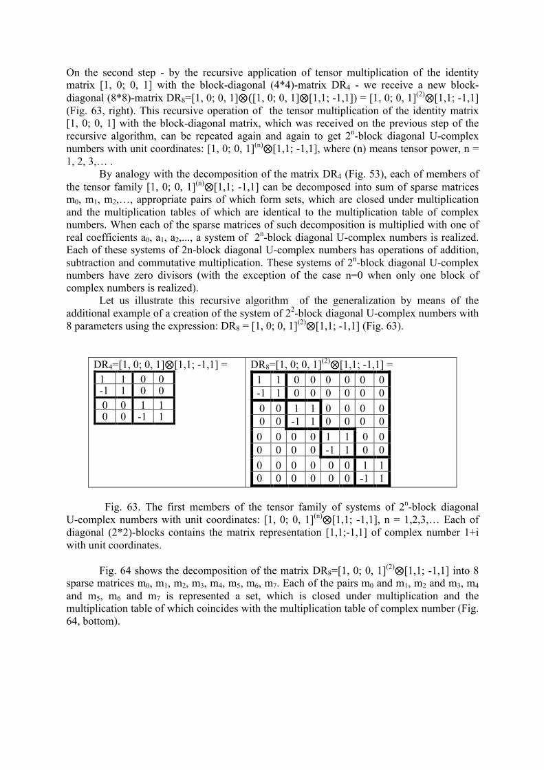
On the second step - by the recursive application of tensor multiplication of the identity matrix [1, 0; 0, 1] with the block-diagonal (4*4)-matrix DR4 - we receive a new block-diagonal (8*8)-matrix DR8=[1, 0; 0, 1]⨂([1, 0; 0, 1]⨂[1,1; -1,1]) = [1, 0; 0, 1](2)⨂[1,1; -1,1] (Fig. 63, right). This recursive operation of the tensor multiplication of the identity matrix [1, 0; 0, 1] with the block-diagonal matrix, which was received on the previous step of the recursive algorithm, can be repeated again and again to get 2n-block diagonal U-complex numbers with unit coordinates: [1, 0; 0, 1](n)⨂[1,1; -1,1], where (n) means tensor power, n = 1, 2, 3,… .

By analogy with the decomposition of the matrix DR4 (Fig. 53), each of members of the tensor family [1, 0; 0, 1](n)⨂[1,1; -1,1] can be decomposed into sum of sparse matrices m0, m1, m2,…, appropriate pairs of which form sets, which are closed under multiplication and the multiplication tables of which are identical to the multiplication table of complex numbers. When each of the sparse matrices of such decomposition is multiplied with one of real coefficients a0, a1, a2,..., a system of 2n-block diagonal U-complex numbers is realized. Each of these systems of 2n-block diagonal U-complex numbers has operations of addition, subtraction and commutative multiplication. These systems of 2n-block diagonal U-complex numbers have zero divisors (with the exception of the case n=0 when only one block of complex numbers is realized).

Let us illustrate this recursive algorithm of the generalization by means of the additional example of a creation of the system of 22-block diagonal U-complex numbers with 8 parameters using the expression: DR8 = [1, 0; 0, 1](2)⨂[1,1; -1,1] (Fig. 63).

DR4=[1, 0; 0, 1]⨂[1,1; -1,1] = 1 1 0 0 -1 1 0 0 0 0 1 1 0 0 -1 1

DR8=[1, 0; 0, 1](2)⨂[1,1; -1,1] = 1 1 0 0 0 0 0 0 -1 1 0 0 0 0 0 0 0 0 1 1 0 0 0 0 0 0 -1 1 0 0 0 0 0 0 0 0 1 1 0 0 0 0 0 0 -1 1 0 0 0 0 0 0 0 0 1 1 0 0 0 0 0 0 -1 1

Fig. 63. The first members of the tensor family of systems of 2n-block diagonal

U-complex numbers with unit coordinates: [1, 0; 0, 1](n)⨂[1,1; -1,1], n = 1,2,3,… Each of diagonal (2*2)-blocks contains the matrix representation [1,1;-1,1] of complex number 1+i with unit coordinates.

Fig. 64 shows the decomposition of the matrix DR8=[1, 0; 0, 1](2)⨂[1,1; -1,1] into 8

sparse matrices m0, m1, m2, m3, m4, m5, m6, m7. Each of the pairs m0 and m1, m2 and m3, m4 and m5, m6 and m7 is represented a set, which is closed under multiplication and the multiplication table of which coincides with the multiplication table of complex number (Fig. 64, bottom).

DR8=[1, 0; 0, 1](2)⨂[1,1; -1,1]=

1 1 0 0 0 0 0 0 -1 1 0 0 0 0 0 0 0 1 1 0 0 0 0 0 0 -1 1 0 0 0 0 0 0 0 0 1 1 0 0 0 0 0 0 -1 1 0 0 0 0 0 0 0 0 1 1 0 0 0 0 0 0 -1 1

=

=

1 0 0 0 0 0 0 0 0 1 0 0 0 0 0 0 0 0 0 0 0 0 0 0 0 0 0 0 0 0 0 0 0 0 0 0 0 0 0 0 0 0 0 0 0 0 0 0 0 0 0 0 0 0 0 0 0 0 0 0 0 0 0 0

+

0 1 0 0 0 0 0 0 -1 0 0 0 0 0 0 0 0 0 0 0 0 0 0 0 0 0 0 0 0 0 0 0 0 0 0 0 0 0 0 0 0 0 0 0 0 0 0 0 0 0 0 0 0 0 0 0 0 0 0 0 0 0 0 0

+

0 0 0 0 0 0 0 0 0 0 0 0 0 0 0 0 0 0 1 0 0 0 0 0 0 0 0 1 0 0 0 0 0 0 0 0 0 0 0 0 0 0 0 0 0 0 0 0 0 0 0 0 0 0 0 0 0 0 0 0 0 0 0 0

+

0 0 0 0 0 0 0 0 0 0 0 0 0 0 0 0 0 0 0 1 0 0 0 0 0 0 -1 0 0 0 0 0 0 0 0 0 0 0 0 0 0 0 0 0 0 0 0 0 0 0 0 0 0 0 0 0 0 0 0 0 0 0 0 0

+

0 0 0 0 0 0 0 0 0 0 0 0 0 0 0 0 0 0 0 0 0 0 0 0 0 0 0 0 0 0 0 0 0 0 0 0 1 0 0 0 0 0 0 0 0 1 0 0 0 0 0 0 0 0 0 0 0 0 0 0 0 0 0 0

+

0 0 0 0 0 0 0 0 0 0 0 0 0 0 0 0 0 0 0 0 0 0 0 0 0 0 0 0 0 0 0 0 0 0 0 0 0 1 0 0 0 0 0 0 -1 0 0 0 0 0 0 0 0 0 0 0 0 0 0 0 0 0 0 0

+

0 0 0 0 0 0 0 0 0 0 0 0 0 0 0 0 0 0 0 0 0 0 0 0 0 0 0 0 0 0 0 0 0 0 0 0 0 0 0 0 0 0 0 0 0 0 0 0 0 0 0 0 0 0 1 0 0 0 0 0 0 0 0 1

+

0 0 0 0 0 0 0 0 0 0 0 0 0 0 0 0 0 0 0 0 0 0 0 0 0 0 0 0 0 0 0 0 0 0 0 0 0 0 0 0 0 0 0 0 0 0 0 0 0 0 0 0 0 0 0 1 0 0 0 0 0 0 -1 0

= m0+m1 +m2+m3 +m4+m5 +m6+m7

* m0 m1

m0 m0 m1

m1 m1 -m0

* m2 m3

m2 m2 m3

m3 m3 -m2

* m4 m5

m4 m4 m5

m5 m5 -m4

* m6 m7

m6 m6 m7

m7 m7 -m6

Fig. 64. Top: the decomposition of the matrix DR8=[1, 0; 0, 1](2)⨂[1,1; -1,1] into 8

sparse matrices m0, m1, m2, m3, m4, m5, m6, m7. Bottom: multiplication tables for the following pairs: m0 and m1; m2 and m3; m4 and m5; m6 and m7.

Taking each of sparse matrices m0, m1, m2, m3, m4, m5, m6, m7 with its own real

coefficients a0, a1, a2,..., we receive the system of 22-block diagonal U-complex numbers: a0*m0+a1*m1+a2*m2+a3*m3+a4*m4+a5*m5+a6*m6+a7*m7 (Fig. 65). This system has operations of addition, subtraction and commutative multiplication and it has zero divisors. Any non-zero member of this system has its inverse number of the same type. Due to this, the operation of division can be defined here by usual manner as multiplication with inverse numbers.

a0 a1 0 0 0 0 0 0 -a1 a0 0 0 0 0 0 0 0 0 a2 a3 0 0 0 0 0 0 -a3 a2 0 0 0 0 0 0 0 0 a4 a5 0 0 0 0 0 0 -a5 a4 0 0 0 0 0 0 0 0 a6 a7 0 0 0 0 0 0 -a7 a6

Fig. 65. The matrix system of 22-block diagonal U-complex numbers In general, by means of such recursive algorithm using the expression

[1, 0; 0, 1](n)⨂[1,1; -1,1], we have constructed the tensor family of 2n-block diagonal U-complex numbers. Parameters a0, a1, a2,... in separate blocks of each of these systems can be functions of time and can be interrelated with each other to model multi-parametrical systems with various interrelations between their parts. Special attention we pay to applications of 2n-block diagonal U-complex numbers for modeling interrelated cyclic processes in living organisms:

• cycles of “life-and-death” of proteins, cells and other parts of organisms; • interpretation of various diseases (including oncological and cardio-vascular) as

consequences of disturbances in interrelations of physiological cycles in accordance with the doctrine of the ancient chronomedicine;

• cycles of activity and rest of physiological sub-systems with applications in medical diagnostics, pharmacology, ergonomics of professions with the change of time zones (pilots, flight attendants, machinists, etc..), acupuncture and eastern chronomedicine in general, sports of highest achievements;

• approaches to study molecular-genetic systems from the standpoint of the chrono-cyclic conception [Petoukhov, 2001];

• theory of hypercycles of M.Eigen and P.Shuster; • study of cycles in cardiac system and respiratory system, • study of the biological clock inside living bodies; • study of cyclic metamorphoses of butterflies and other organisms; • ensembles of cyclic processes in the field of Artificial Life (ALife), etc.

Beside this, 2n-block diagonal U-complex numbers can be applied also to model interrelated cyclic processes in growing multi-parametrical systems in digital communications, devices of artificial intelligence, physics, economics, finances, engineering, biotechnology, etc.

The system of complex numbers plays significant role in different branches of modern science and technology. One can hope that systems of 2n-block diagonal U-complex numbers will be also useful not only in algebraic biology but also in other fields of science and technology. It seems interesting to develop the theory of functions of several U-complex variables by analogy with the existing theory of functions of several complex variables.

One can mention else the following additional aspect. Till now we focused our attention on the matrix R40 (Fig. 59) of two quadrants along the main diagonal of the matrix R4 from Fig. 1. Now let us pay our attention to the matrix R41 (Fig. 59) of two quadrants along the second diagonal of the matrix R4. As it was mentioned above, both quadrants along the second diagonal are mirror-antisymmetric concerning both quadrants along the main diagonal in relation of the middle horizontal line of R4. Taking this into account, let us

consider the mirror-antisymmetric analog W of 2-block diagonal U-complex numbers S from Fig. 60. Fig. 66 shows that the square of this matrix W2 is again 2-block diagonal U-complex numbers, where each of non-zero coordinates is a combination of all 4 parameters a0, a1, a2 and a3. (It is interesting that in the block-diagonal matrix W2 the upper diagonal block represents complex number (a0*a2+a1*a3)+i*(a1*a2-a0*a3) and the lower diagonal block represents the conjugate complex number (a0*a2+a1*a3)-i*(a1*a2-a0*a3)). The similar relation is true for 2n-block diagonal U-complex numbers and their mirror-antisymmetric analogues.

W = [0, 0, a3, -a2 0, 0, -a2, -a3 a1, -a0, 0, 0 -a0, -a1, 0, 0]

W2 = [ a0*a2+a1*a3, a1*a2-a0*a3, 0, 0 -(a1*a2-a0*a3), a0*a2+a1*a3, 0, 0 0, 0, a0*a2+a1*a3, -(a1*a2-a0*a3) 0, 0, (a1*a2-a0*a3), a0*a2 + a1*a3]

Fig. 66. The mirror-antisymmetric analogue W of 2-block diagonal U-complex

numbers S from Fig. 60. Its square W2 is again 2-block diagonal U-complex numbers.

Let us return to the recursive algorithm with the expression [1, 0; 0, 1](n)⨂[1,1; -1,1]. This algorithm can be extended to cases of expressions [1, 0; 0, 1](n)⨂M, where the square matrix M represents not the complex number with unit coordinates [1,1; -1,1] but other kinds of complex and hypercomplex numbers with unit coordinates: split-complex numbers (their synonyms are double numbers and hyperbolic numbers), dual numbers, quaternions of Hamilton, split-quaternions of Cockle, octonions, etc. In these cases we meet with the following kinds of 2n-block diagonal U-numbers:

• 2n-block diagonal U-double numbers; • 2n-block diagonal U-dual numbers; • 2n-block diagonal U-quaternions; • 2n-block diagonal U-split-quaternions, etc.

Algebraic properties of these kinds of 2n-block diagonal U-numbers will be published later.

The introduced systems of multi-block U-numbers define new – for mathematical natural sciences - types of multi-dimensional spaces (U-numerical spaces), some of which are vector spaces with special interrelations of their vectors.

What one can say about difference between systems of multi-block U-complex numbers and a corresponding set of separate complex numbers, which can be also applied to model a behavior of multi-parametrical systems? Firstly, multi-block U-complex numbers operate inside appropriate multi-dimensional spaces, where - in cases of vector spaces – Descarte’s systems of coordinates can be introduced with certain orders of coordinate axes, appropriate orders of components of multi-dimensional vectors, appropriate numerations of sub-spaces and appropriate interrelations between multi-dimensional vectors. In a simple set of separate complex numbers such order of its members is absent. Secondly, the difference exists in relation to the operation of tensor multiplication, which is very essential to model multi-parametrical systems with increasing quantities of parameters: a result of tensor multiplication of two multi-block U-complex numbers differs from a result of tensor multiplication of two separate complex numbers. Similar differences are true for systems of multi-block U-split-complex numbers, etc.

In our approach we intensively used tensor multiplication of matrices taking into account, in particular, the following facts: DNA-‐molecules belong to the quantum mechanical level, but in quantum mechanics the tensor multiplication is the important operation: when considering a quantum system consisting of two subsystems, the whole space of states is constructed in the form of tensor product of their states.

Of separate interest are multi-block U-numbers with different types of multidimensional numbers in separate blocks (symbiotic U-numbers). In these cases corresponding multi-dimensional spaces can be called as symbiotic spaces.

Our results of researches in the field of matrix genetics additionally attract an attention to matrix operators in a form of 2n-block diagonal united operators, for example, 2n-block diagonal united Hadamard matrices for spectral analysis in different sub-spaces of multi-dimensional space.

17. TETRA-GROUPS OF OLIGONUCLEOTIDES AND RULES OF LONG NUCLEOTIDE SEQUENCES

By unknown reasons, the Nature has chosen the DNA- and RNA-alphabets, each of which contains only 4 letters (A, T, C, G in DNA and A, U, C, G in RNA) with complementary relations among them. In other words, in these basic cases of DNA and RNA, the Nature uses the tetra-groups of letters. In this Section we study a role of special tetra-groups of oligonucleotides in long nucleotide sequences. We use separations of each of complete sets of oligonucleotides (42 doublets, 43 triplets, …, 4n n-plets) into tetra-groups of equivalency, criterium of which are based on these 4 letters, to study hidden symmetries in long nucleotide sequences. The tetra-group of mononucleotides A, T, C, G is the limiting degenerate case of the introduced set of tetra-groups of oligonucleotides.

One can remind that many authors devoted their works from the middle of XX century to searching of hidden regularities or symmetry principles in long nucleotide sequences. The Chargaff's first parity rule speaks that in any double-stranded DNA segment, the number of occurrences (or frequencies) of adenine A and thymine T are equal, and so are the frequencies of cytosine C and guanine G [Chargaff, 1951, 1971]. This rule was used by Watson and Crick to support their famous DNA double-helix structure model. Chargaff also perceived that the parity rule approximately holds in the single-stranded DNA segment for long nucleotide sequences. This last rule is known as Chargaff’s second parity rule (CSPR), and it has been confirmed in several organisms [Mitchell & Bride, 2006]. Originally, CSPR is meant to be valid only to mononucleotide frequencies (that is quantities of monoplets) in the single-stranded DNA. “But, it occurs that oligonucleotide frequencies follow a generalized Chargaff’s second parity rule (GCSPR) where the frequency of an oligonucleotide is approximately equal to its complement reverse oligonucleotide frequency [Prahbu, 1993]. This is known in the literature as the Symmetry Principle” [Yamagishi, Herai, 2011, p. 2]. The work [Prahbu, 1993] shows the implementation of the Symmetry Principle in long DNA-sequences for cases of complementary reverse n-plets with n = 2, 3, 4, 5 at least. (In literature, a few synonimes of the term "n-plets" are used: n-tuples, n-words or n-mers). These parity rules for long nucleotide sequences are analysed and discussed in many works [Bell, Forsdyke, 1999; Chargaff, 1971, 1975; Dong, Cuticchia, 2001; Forsdyke, 2002; Forsdyke, Bell, 2004; Mitchell, Bridge, 2006; Prabhu, 1993; Yamagishi, Herai, 2011].

These parity rules (or rules of equality), including generalized Chargaff’s second parity rule, concerns the equality of frequencies of two separate mononucleotides or two separate oligonucleotides: the equality of frequencies of adenine and thymine, the equality of frequences of the doublet CA and its complement reverse doublet TG, etc. By contrast to this,

to study hidden symmetries in long nucleotide sequences, we apply a comparative analysis of equalities not for frequencies of separate oligonucleotides but for aggregated frequencies (or collective frequences) of oligonucleotides from each of 4 equal subsets, which are formed by means of a certain criterion of equivalency. More precisely, first of all, we divide each of complete alphabets of n-plets into 4 subsets with 4n-1 n-plets in each by the criterion of the same first letter in each n-plet. The complect of these four subsets is called the tetra-group of this equivalence. The sum of the frequencies of all oligonucleotides of each subset is called the collective frequency of a given subset in the considered long sequence of nucleotides.

For example, in the case of the alphabet of 16 doublets, the tetra-group of this equivalence is formed with 4 equivalent doublets in each of its 4 collective members:

-‐ the first collective member: AA=AC=AG=AT; -‐ the second collective member: TC=TA=TT=TG; -‐ the third collective member: CC=CA=CT=CG; (13) -‐ the fourth collective member: GC=GA=GT=GG.

Taking into account the complementarities of bases A-T and C-G in DNA, two subsets of oligonuclotides with the complementary first letters are called "complementary subsets by the first letter". For example, in the described tetra-group of doublets (13) the first and the second collective members are complementary each other by the first letter (A and T are complemetary); similar is true for the third and fourth collective members (their first letters C and G are complementary).

In long nucleotide sequences, each of oligonucleotides has its individual frequency F of existence, which can be denoted, for example, for doublets as F(CC), F(CA), etc. We denote collective frequencies for each of 4 collective members of the tetra-group as Fn(C), Fn(G), Fn(A) and Fn(T), where the index n = 1, 2, 3, 4,… means the length of considered oligonucleotides (that is n-plets). For example, in the case of the described tetra-group of 16 doublets (13), we study collective frequencies F2(C), F2(G), F2(A) and F2(T):

-‐ F2(A) = F(AA) + F(AC) + F(AG) + F(AT), -‐ F2(T) = F(TC) + F(TA) + F(TT) + F(TG). -‐ F2(C) = F(CC) + F(CA) + F(CT) + F(CG), (14) -‐ F2(G) = F(GC) + F(GA) + F(GT) + F(GG),

Simultaneously we study another kind of tetra-groups of equivalence by the criterion

of the same last letter in n-plets. For example in the case of 16 doublets, the tetra-group of this «reverse» equivalence is the following:

-‐ the first collective member: AA=CA=GA=TA; -‐ the second collective member: CT=AT=TT=GT; -‐ the third collective member: CC=AC=TC=GC; (15) -‐ the fourth collective member: CG=AG=TG=GG.

Two subsets of oligonuclotides with the complementary last letters are called

"complementary subsets by the last letter". For example, in the described tetra-group of doublets (15) the first and the second collective members are complementary each other by the last letter (A and T); similar is true for the third and fourth collective members (their last letters C and G are complementary).

We denote collective frequencies for each of 4 collective members of this “reverse” tetra-group as FRn(C), FRn(G), FRn(A) and FRn(T), where the index n = 1, 2, 3, 4,… means

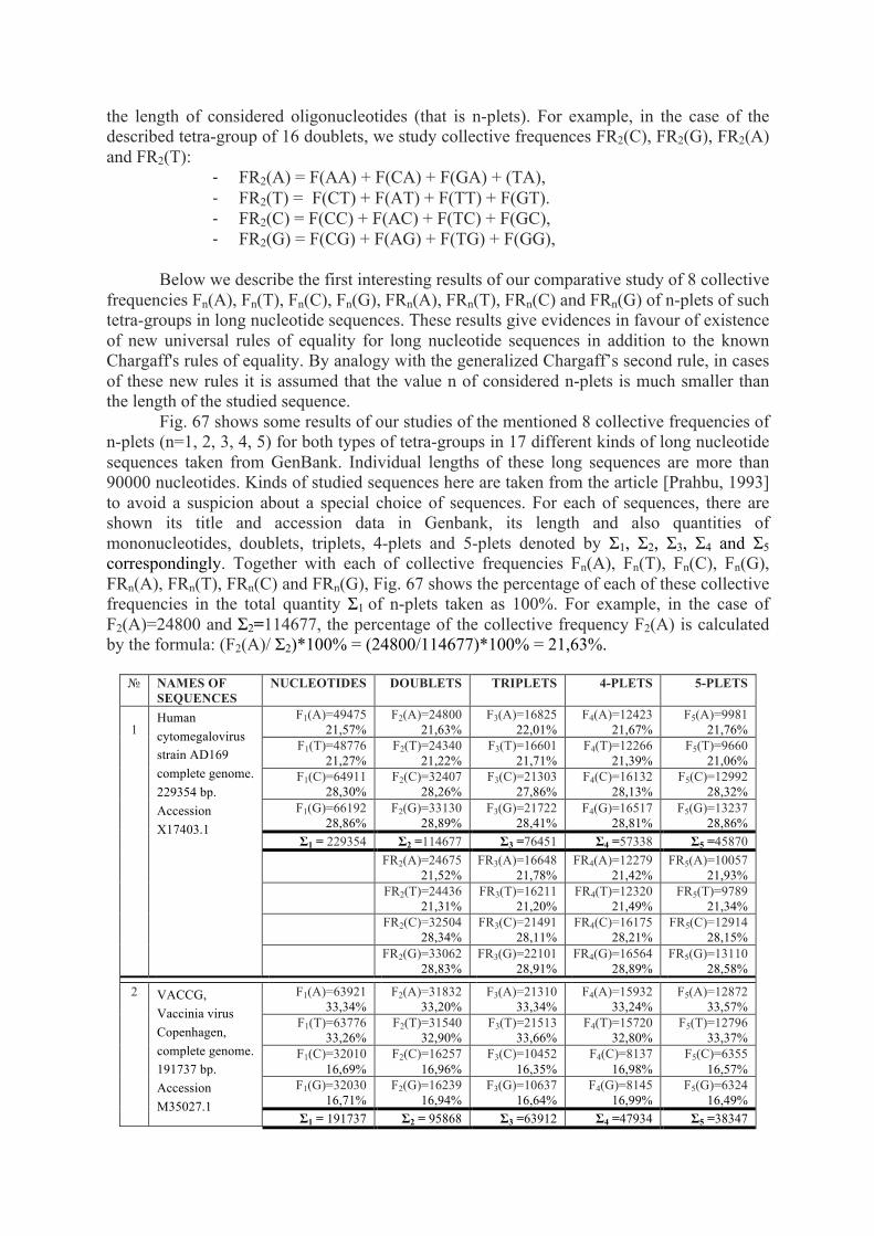
the length of considered oligonucleotides (that is n-plets). For example, in the case of the described tetra-group of 16 doublets, we study collective frequences FR2(C), FR2(G), FR2(A) and FR2(T):

-‐ FR2(A) = F(AA) + F(CA) + F(GA) + (TA), -‐ FR2(T) = F(CT) + F(AT) + F(TT) + F(GT). -‐ FR2(C) = F(CC) + F(AC) + F(TC) + F(GC), -‐ FR2(G) = F(CG) + F(AG) + F(TG) + F(GG),

Below we describe the first interesting results of our comparative study of 8 collective

frequencies Fn(A), Fn(T), Fn(C), Fn(G), FRn(A), FRn(T), FRn(C) and FRn(G) of n-plets of such tetra-groups in long nucleotide sequences. These results give evidences in favour of existence of new universal rules of equality for long nucleotide sequences in addition to the known Chargaff's rules of equality. Вy analogy with the generalized Chargaff’s second rule, in cases of these new rules it is assumed that the value n of considered n-plets is much smaller than the length of the studied sequence.

Fig. 67 shows some results of our studies of the mentioned 8 collective frequencies of n-plets (n=1, 2, 3, 4, 5) for both types of tetra-groups in 17 different kinds of long nucleotide sequences taken from GenBank. Individual lengths of these long sequences are more than 90000 nucleotides. Kinds of studied sequences here are taken from the article [Prahbu, 1993] to avoid a suspicion about a special choice of sequences. For each of sequences, there are shown its title and accession data in Genbank, its length and also quantities of mononucleotides, doublets, triplets, 4-plets and 5-plets denoted by Σ1, Σ2, Σ3, Σ4 and Σ5 correspondingly. Together with each of collective frequencies Fn(A), Fn(T), Fn(C), Fn(G), FRn(A), FRn(T), FRn(C) and FRn(G), Fig. 67 shows the percentage of each of these collective frequencies in the total quantity Σ1 of n-plets taken as 100%. For example, in the case of F2(A)=24800 and Σ2=114677, the percentage of the collective frequency F2(A) is calculated by the formula: (F2(A)/ Σ2)*100% = (24800/114677)*100% = 21,63%.

№ NAMES OF SEQUENCES

NUCLEOTIDES DOUBLETS TRIPLETS 4-PLETS 5-PLETS

1

Human cytomegalovirus strain AD169 complete genome. 229354 bp. Accession X17403.1

F1(A)=49475 21,57%

F2(A)=24800 21,63%

F3(A)=16825 22,01%

F4(A)=12423 21,67%

F5(A)=9981 21,76%

F1(T)=48776 21,27%

F2(T)=24340 21,22%

F3(T)=16601 21,71%

F4(T)=12266 21,39%

F5(T)=9660 21,06%

F1(C)=64911 28,30%

F2(C)=32407 28,26%

F3(C)=21303 27,86%

F4(C)=16132 28,13%

F5(C)=12992 28,32%

F1(G)=66192 28,86%

F2(G)=33130 28,89%

F3(G)=21722 28,41%

F4(G)=16517 28,81%

F5(G)=13237 28,86%

Σ1 = 229354 Σ2 =114677 Σ3 =76451 Σ4 =57338 Σ5 =45870 FR2(A)=24675

21,52% FR3(A)=16648

21,78% FR4(A)=12279

21,42% FR5(A)=10057

21,93% FR2(T)=24436

21,31% FR3(T)=16211

21,20% FR4(T)=12320

21,49% FR5(T)=9789

21,34% FR2(C)=32504

28,34% FR3(C)=21491

28,11% FR4(C)=16175

28,21% FR5(C)=12914

28,15% FR2(G)=33062

28,83% FR3(G)=22101

28,91% FR4(G)=16564

28,89% FR5(G)=13110

28,58%

2

VACCG, Vaccinia virus Copenhagen, complete genome. 191737 bp. Accession M35027.1

F1(A)=63921 33,34%

F2(A)=31832 33,20%

F3(A)=21310 33,34%

F4(A)=15932 33,24%

F5(A)=12872 33,57%

F1(T)=63776 33,26%

F2(T)=31540 32,90%

F3(T)=21513 33,66%

F4(T)=15720 32,80%

F5(T)=12796 33,37%

F1(C)=32010 16,69%

F2(C)=16257 16,96%

F3(C)=10452 16,35%

F4(C)=8137 16,98%

F5(C)=6355 16,57%

F1(G)=32030 16,71%

F2(G)=16239 16,94%

F3(G)=10637 16,64%

F4(G)=8145 16,99%

F5(G)=6324 16,49%

Σ1 = 191737 Σ2 = 95868 Σ3 =63912 Σ4 =47934 Σ5 =38347

FR2(A)=32088 33,47%

FR3(A)=21337 33,38%

FR4(A)=16024 33,43%

FR5(A)=12711 33,15%

FR2(T)=32236 33,63%

FR3(T)=21239 33,23%

FR4(T)=16104 33,60%

FR5(T)=12847 33,50%

FR2(C)=15753 16,43%

FR3(C)=11007 17,22%

FR4(C)=7871 16,42%

FR5(C)=6307 16,45%

FR2(G)=15791 16,47%

FR3(G)=10329 16,16%

FR4(G)=7935 16,55%

FR5(G)=6482 16,90%

3

MPOMTCG, Marchantia paleacea isolate A 18 mitochondrion, complete genome. 186609 bp. Accession M68929.1

F1(A)=53206 28,51%

F2(A)=26575 28,48%

F3(A)=17874 28,73%

F4(A)=13285 28,48%

F5(A)=10665 28,58%

F1(T)=54264 29,08%

F2(T)=27190 29,14%

F3(T)=17831 28,67%

F4(T)=13477 28,89%

F5(T)=10782 28,89%

F1(C)=39215 21,01%

F2(C)=19603 21,01%

F3(C)=12979 20,87%

F4(C)=9882 21,18%

F5(C)=7742 20,74%

F1(G)=39924 21,39%

F2(G)=19936 21,37%

F3(G)=13519 21,73%

F4(G)=10008 21,45%

F5(G)=8132 21,79%

Σ1 = 186609 Σ2 = 93304 Σ3 =62203 Σ4 =46652 Σ5 =37321 FR2(A)=26631

28,54% FR3(A)=17607

28,31% FR4(A)=13207

28,31% FR5(A)=10504

28,15% FR2(T)=27073

29,02% FR3(T)=18339

29,48% FR4(T)=13600

29,15% FR5(T)=10860

29,10% FR2(C)=19612

21,02% FR3(C)=13159

21,15% FR4(C)=9866

21,15% FR5(C)=8021

21,49% FR2(G)=19988

21,42% FR3(G)=13098

21,06% FR4(G)=9979

21,39% FR5(G)=7936

21,26%

4

HS4B958RAJ, Epstein-Barr virus. 184113 bp. Accession M80517.1

F1(A)=36002 19,55%

F2(A)=18098 19,66%

F3(A)=11910 19,41%

F4(A)=9044 19,65%

F5(A)=7210 19,58%

F1(T)=37665 20,46%

F2(T)=18887 20,52%

F3(T)=12160 19,81%

F4(T)=9394 20,41%

F5(T)=7571 20,56%

F1(C)=55824 30,32%

F2(C)=27823 30,22%

F3(C)=19144 31,19%

F4(C)=13990 30,39%

F5(C)=11162 30,31%

F1(G)=54622 29,67%

F2(G)=27248 29,60%

F3(G)=18157 29,59%

F4(G)=13600 29,55%

F5(G)=10879 29,54%

Σ1 = 184113 Σ2 = 92056 Σ3 =61371 Σ4 =46028 Σ5 =36822 FR2(A)=17903

19,45% FR3(A)=12495

20,36% FR4(A)=9145

19,87% FR5(A)=7178

19,49% FR2(T)=18778

20,40% FR3(T)=12940

21,08% FR4(T)=9499

20,64% FR5(T)=7583

20,59% FR2(C)=28001

30,42% FR3(C)=18163

29,60% FR4(C)=13640

29,63% FR5(C)=11145

30,27% FR2(G)=27374

29,74% FR3(G)=17773

28,96% FR4(G)=13744

29,86% FR5(G)=10916

29,65%

5

Nicotiana tabacum chloroplast genome DNA. 155943 bp. Accession Z00044.2

F1(A)=47860 30,69%

F2(A)=23952 30,72%

F3(A)=16025 30,83%

F4(A)=12043 30,89%

F5(A)=9661 30,98%

F1(T)=49064 31,46%

F2(T)=24497 31,42%

F3(T)=16460 31,67%

F4(T)=12313 31,58%

F5(T)=9743 31,24%

F1(C)=30014 19,25%

F2(C)=15095 19,36%

F3(C)=9974 19,19%

F4(C)=7452 19,12%

F5(C)=5997 19,23%

F1(G)=29005 18,60%

F2(G)=14427 18,50%

F3(G)=9522 18,32%

F4(G)=7177 18,41%

F5(G)=5787 18,56%

Σ1 = 155943 Σ2 = 77971 Σ3 =51981 Σ4 =38985 Σ5 =31188 FR2(A)=23907

30,66% FR3(A)=15602

30,01% FR4(A)=11867

30,44% FR5(A)=9490

30,43% FR2(T)=24567

31,51% FR3(T)=16480

31,70% FR4(T)=12375

31,74% FR5(T)=9891

31,71% FR2(C)=14919

19,13% FR3(C)=10077

19,39% FR4(C)=7433

19,07% FR5(C)=5970

19,14% FR2(G)=14578

18,70% FR3(G)=9822

18,90% FR4(G)=7310

18,75% FR5(G)=5837

18,72%

6

Equine herpesvirus 1

F1(A)=32616 21,71%

F2(A)=16273 21,66%

F3(A)=11331 22,63%

F4(A)=8082 21,52%

F5(A)=6480 21,57%

F1(T)=32482 F2(T)=16191 F3(T)=10871 F4(T)=8106 F5(T)=6514

strain Ab4, complete genome. 150224 bp . Accession AY665713.1

21,62% 21,56% 21,71% 21,58% 21,68% F1(C)=43173

28,74% F2(C)=21746

28,95% F3(C)=14287

28,53% F4(C)=10735

28,58% F5(C)=8646

28,78% F1(G)=41953

27,93% F2(G)=20902

27,83% F3(G)=13585

27,13% F4(G)=10633

28,31% F5(G)=8404

27,97% Σ1 = 150224 Σ2 = 75112 Σ3 =50074 Σ4 =37556 Σ5 =30044

FR2(A)=16343 21,76%

FR3(A)=10938 21,84%

FR4(A)=8222 21,89%

FR5(A)=6542 21,77%

FR2(T)=16291 21,69%

FR3(T)=10822 21,61%

FR4(T)=8147 21,69%

FR5(T)=6471 21,54%

FR2(C)=21427 28,53%

FR3(C)=13997 27,95%

FR4(C)=10724 28,55%

FR5(C)=8723 29,03%

FR2(G)=21051 28,03%

FR3(G)=14317 28,59%

FR4(G)=10463 27,86%

FR5(G)=8308 27,65%

7

Equine herpesvirus 1 strain Ab4, complete genome. 150224 bp. Accession AY665713.1

F1(A)=32616 21,71%

F2(A)=16273 21,66%

F3(A)=11331 22,63%

F4(A)=8082 21,52%

F5(A)=6480 21,57%

F1(T)=32482 21,62%

F2(T)=16191 21,56%

F3(T)=10871 21,71%

F4(T)=8106 21,58%

F5(T)=6514 21,68%

F1(C)=43173 28,74%

F2(C)=21746 28,95%

F3(C)=14287 28,53%

F4(C)=10735 28,58%

F5(C)=8646 28,78%

>G>=41953 27,93%

F2(G)=20902 27,83%

F3(G)=13585 27,13%

F4(G)=10633 28,31%

F5(G)=8404 27,97%

Σ1 = 150224 Σ2 = 75112 Σ3 =50074 Σ4 =37556 Σ5 =30044 FR2(A)=16343

21,76% FR3(A)=10938

21,84% FR4(A)=8222

21,89% FR5(A)=6542

21,77% FR2(T)=16291

21,69% FR3(T)=10822

21,61% FR4(T)=8147

21,69% FR5(T)=6471

21,54% FR2(C)=21427

28,53% FR3(C)=13997

27,95% FR4(C)=10724

28,55% FR5(C)=8723

29,03% FR2(G)=21051

28,03% FR3(G)=14317

28,59% FR4(G)=10463

27,86% FR5(G)=8308

27,65%

8 Oryza sativa cultivar TN1 chloroplast, complete genome. 134502 bp. Accession NC_031333.1

F1(A)=41231 30,65%

F2(A)=20572 30,59%

F3(A)=13637 30,42%

F4(A)=10209 30,36%

F5(A)=8302 30,86%

F1(T)=40818 30,35%

F2(T)=20391 30,32%

F3(T)=13675 30,50%

F4(T)=10159 30,21%

F5(T)=8094 30,09%

F1(C)=26129 19,43%

F2(C)=13035 19,38%

F3(C)=8815 19,66%

F4(C)=6576 19,56%

F5(C)=5341 19,86%

F1(G)=26324 19,57%

F2(G)=13253 19,71%

F3(G)=8707 19,42%

F4(G)=6681 19,87%

F5(G)=5163 19,19%

Σ1 = 134502 Σ2 = 67251 Σ3 =44834 Σ4 =33625 Σ5 =26900 FR2(A)=20659

30,72% FR3(A)=13722

30,61% FR4(A)=10286

30,59% FR5(A)=8197

30,47% FR2(T)=20427

30,37% FR3(T)=13382

29,85% FR4(T)=10249

30,48% FR5(T)=8129

30,22% FR2(C)=13094

19,47% FR3(C)=8704

19,41% FR4(C)=6596

19,62% FR5(C)=5307

19,73% FR2(G)=13071

19,44% FR3(G)=9026

20,13% FR4(G)=6494

19,31% FR5(G)=5267

19,58%

9 IH1CG, Ictalurid herpesvirus 1 strain Auburn 1, complete genome. 134226 bp. Accession M75136.2

F1(A)=28727 21,40%

F2(A)=14299 21,31%

F3(A)=9855 22,03%

F4(A)=7148 21,30%

F5(A)=5795 21,59%

F1(T)=30025 22,37%

F2(T)=15047 22,42%

F3(T)=10633 23,77%

F4(T)=7535 22,46%

F5(T)=5969 22,24%

F1(C)=37767 28,14%

F2(C)=18943 28,23%

F3(C)=12066 26,97%

F4(C)=9436 28,12%

F5(C)=7480 27,86%

F1(G)=37707 28,09%

F2(G)=18824 28,05%

F3(G)=12188 27,24%

F4(G)=9437 28,12%

F5(G)=7601 28,31%

Σ1 = 134226 Σ2 = 67113 Σ3 =44742 Σ4 =33556 Σ5 =26845 FR2(A)=14428

21,50% FR3(A)=9954

22,25% FR4(A)=7233

21,56% FR5(A)=5756

21,44% FR2(T)=14978

22,32% FR3(T)=9795

21,89% FR4(T)=7506

22,37% FR5(T)=5865

21,85% FR2(C)=18824

28,05% FR3(C)=12106

27,06% FR4(C)=9413

28,05% FR5(C)=7682

28,62%

FR2(G)=18883 28,14%

FR3(G)=12887 28,80%

FR4(G)=9404 28,02%

FR5(G)=7542 28,09%

10

Human herpesvirus 3 isolate 667/2005, complete genome. 124884 bp. Accession JN704693.1

F1(A)=33782 27,05%

F2(A)=16995 27,22%

F3(A)=11327 27,21%

F4(A)=8467 27,12%

F5(A)=6724 26,92%

F1(T)=33623 26,92%

F2(T)=16785 26,88%

F3(T)=11586 27,83%

F4(T)=8445 27,05%

F5(T)=6767 27,09%

F1(C)=29295 23,46%

F2(C)=14590 23,37%

F3(C)=9512 22,85%

F4(C)=7336 23,50%

F5(C)=5826 23,33%

F1(G)=28184 22,57%

F2(G)=14072 22,54%

F3(G)=9203 22,11%

F4(G)=6973 22,33%

F5(G)=5659 22,66%

Σ1 = 124884 Σ2 = 62442 Σ3 =41628 Σ4 =31221 Σ5 =24976 FR2(A)=16787

26,88% FR3(A)=11358

27,28% FR4(A)=8424

26,98% FR5(A)=6753

27,04% FR2(T)=16838

26,97% FR3(T)=10995

26,41% FR4(T)=8390

26,87% FR5(T)=6807

27,25% FR2(C)=14705

23,55% FR3(C)=9969

23,95% FR4(C)=7318

23,44% FR5(C)=5846

23,41% FR2(G)=14112

22,60% FR3(G)=9306

22,36% FR4(G)=7089

22,71% FR5(G)=5570

22,30%

11

Marchantia paleacea chloroplast genome DNA. 121024 bp. Accession X04465.1

F1(A)=42896 35,44%

F2(A)=21385 35,34%

F3(A)=14349 35,57%

F4(A)=10739 35,49%

F5(A)=8517 35,19%

F1(T)=43263 35,75%

F2(T)=21703 35,87%

F3(T)=14637 36,28%

F4(T)=10870 35,93%

F5(T)=8677 35,85%

F1(C)=17309 14,30%

F2(C)=8677 14,34%

F3(C)=5687 14,10%

F4(C)=4340 14,34%

F5(C)=3448 14,25%

F1(G)=17556 14,51%

F2(G)=8747 14,45%

F3(G)=5668 14,05%

F4(G)=4307 14,24%

F5(G)=3562 14,72%

Σ1 = 121024 Σ2 = 60512 Σ3 =40341 Σ4 =30256 Σ5 =24204 FR2(A)=21511

35,55% FR3(A)=14273

35,38% FR4(A)=10729

35,46% FR5(A)=8552

35,33% FR2(T)=21560

35,63% FR3(T)=13879

34,40% FR4(T)=10745

35,51% FR5(T)=8680

35,86% FR2(C)=8632

14,26% FR3(C)=5965

14,79% FR4(C)=4344

14,36% FR5(C)=3436

14,20% FR2(G)=8809

14,56% FR3(G)=6224

15,43% FR4(G)=4438

14,67% FR5(G)=3536

14,61%

12

Escherichia coli strain PSUO78 plasmid pPSUO78_1, complete sequence. 132464 bp. Accession CP012113.1

F1(A)=33030 24,94%

F2(A)=16477 24,88%

F3(A)=11106 25,15%

F4(A)=8304 25,08%

F5(A)=6592 24,88%

F1(T)=33824 25,53%

F2(T)=16910 25,53%

F3(T)=11340 25,68%

F4(T)=8526 25,75%

F5(T)=6907 26,07%

F1(C)=34062 25,71%

F2(C)=17075 25,78%

F3(C)=11321 25,64%

F4(C)=8428 25,45%

F5(C)=6813 25,72%

F1(G)=31548 23,82%

F2(G)=15770 23,81%

F3(G)=10387 23,52%

F4(G)=7858 23,73%

F5(G)=6180 23,33%

Σ1 = 132464 Σ2 = 66232 Σ3 =44154 Σ4 =33116 Σ5 =26492 FR2(A)=16553

24,99% FR3(A)=10821

24,51% FR4(A)=8357

25,24% FR5(A)=6595

24,89% FR2(T)=16914

25,54% FR3(T)=11239

25,45% FR4(T)=8423

25,43% FR5(T)=6691

25,26% FR2(C)=16987

25,65% FR3(C)=11592

26,25% FR4(C)=8509

25,69% FR5(C)=6805

25,69% FR2(G)=15778

23,82% FR3(G)=10502

23,78% FR4(G)=7827

23,64% FR5(G)=6401

24,16%

13

HSIULR, Human herpesvirus 1 complete genome. 152261 bp. Accession X14112.1

F1(A)=24240 15,92%

F2(A)=12192 16,01%

F3(A)=7949 15,66%

F4(A)=6121 16,08%

F5(A)=4926 16,18%

F1(T)=24050 15,80%

F2(T)=11941 15,69%

F3(T)=7848 15,46%

F4(T)=5945 15,62%

F5(T)=4862 15,97%

F1(C)=51458 33,80%

F2(C)=25758 33,83%

F3(C)=17447 34,38%

F4(C)=12906 33,91%

F5(C)=10344 33,97%

F1(G)=52513 34,49%

F2(G)=26239 34,47%

F3(G)=17509 34,50%

F4(G)=13093 34,40%

F5(G)=10320 33,89%

Σ1 = 152261 Σ2 = 76130 Σ3 =50753 Σ4 =38065 Σ5 =30452

FR2(A)=12048 15,83%

FR3(A)=8234 16,22%

FR4(A)=5969 15,68%

FR5(A)=4875 16,01%

FR2(T)=12109 15,91%

FR3(T)=8365 16,48%

FR4(T)=6048 15,89%

FR5(T)=4802 15,77%

FR2(C)=25699 33,76%

FR3(C)=16828 33,16%

FR4(C)=12818 33,67%

FR5(C)=10272 33,73%

FR2(G)=26274 34,51%

FR3(G)=17326 34,14%

FR4(G)=13230 34,76%

FR5(G)=10503 34,49%

14 HUMNEUROF, Human oligodendrocyte myelin glycoprotein (OMG) exons 1-2; neurofibromatosis 1 (NF1) exons 28-49; ecotropic viral integration site 2B (EVI2B) exons 1-2; ecotropic viral integration site 2A (EVI2A) exons 1-2; adenylate kinase (AK3) exons 1-2. 100849 bp. Accession L05367.1

F1(A)=30346 30,09%

F2(A)=15271 30,29%

F3(A)=10157 30,21%

F4(A)=7636 30,29%

F5(A)=5978 29,64%

F1(T)=32481 32,21%

F2(T)=16175 32,08%

F3(T)=10746 31,97%

F4(T)=8030 31,85%

F5(T)=6570 32,57%

F1(C)=18635 18,48%

F2(C)=9390 18,62%

F3(C)=6302 18,75%

F4(C)=4727 18,75%

F5(C)=3709 18,39%

F1(G)=19387 19,22%

F2(G)=9588 19,01%

F3(G)=6411 19,07%

F4(G)=4819 19,11%

F5(G)=3912 19,40%

Σ1 = 100849 Σ2 = 50424 Σ3 =33616 Σ4 =25212 Σ5 =20169 FR2(A)=15075

29,90% FR3(A)=10134

30,15% FR4(A)=7523

29,84% FR5(A)=6125

30,37% FR2(T)=16306

32,34% FR3(T)=10865

32,32% FR4(T)=8159

32,36% FR5(T)=6502

32,24% FR2(C)=9245

18,33% FR3(C)=6167

18,35% FR4(C)=4621

18,33% FR5(C)=3630

18,00% FR2(G)=9798

19,43% FR3(G)=6450

19,19% FR4(G)=4909

19,47% FR5(G)=3912

19,40%

15 Podospora anserina mitochondrion, complete genome. 100314 bp. Accession NC_001329.3

F1(A)=35804 35,69%

F2(A)=17906 35,70%

F3(A)=11917 35,64%

F4(A)=8814 35,15%

F5(A)=7101 35,40%

F1(T)=34358 34,25%

F2(T)=17236 34,36%

F3(T)=11802 35,30%

F4(T)=8693 34,66%

F5(T)=6967 34,73%

F1(C)=13428 13,39%

F2(C)=6669 13,30%

F3(C)=4415 13,20%

F4(C)=3413 13,61%

F5(C)=2614 13,03%

F1(G)=16724 16,67%

F2(G)=8346 16,64%

F3(G)=5304 15,86%

F4(G)=4158 16,58%

F5(G)=3380 16,85%

Σ1 = 100314 Σ2 = 50157 Σ3 =33438 Σ4 =25078 Σ5 =20062 FR2(A)=17898

35,68% FR3(A)=11726

35,07% FR4(A)=8922

35,58% FR5(A)=7261

36,19% FR2(T)=17122

34,14% FR3(T)=11546

34,53% FR4(T)=8572

34,18% FR5(T)=6792

33,86% FR2(C)=6759

13,48% FR3(C)=4565

13,65% FR4(C)=3415

13,62% FR5(C)=2700

13,46% FR2(G)=8378

16,70% FR3(G)=5601

16,75% FR4(G)=4169

16,62% FR5(G)=3309

16,49%

16 HUMTCRADCV, Human T-cell receptor genes (Human Tcr-C-delta gene, exons 1-4; Tcr-V-delta gene, exons 1-2;

F1(A)=28063 28,74%

F2(A)=13947 28,57%

F3(A)=9319 28,64%

F4(A)=6869 28,14%

F5(A)=5662 29,00%

F1(T)=26383 27,02%

F2(T)=13185 27,01%

F3(T)=8723 26,80%

F4(T)=6622 27,13%

F5(T)=5189 26,57%

F1(C)=20949 21,46%

F2(C)=10479 21,47%

F3(C)=6987 21,47%

F4(C)=5254 21,53%

F5(C)=4242 21,72%

F1(G)=22235 22,77%

F2(G)=11204 22,95%

F3(G)=7514 23,09%

F4(G)=5662 23,20%

F5(G)=4433 22,70%

Σ1 = 97630 Σ2 = 48815 Σ3 =32543 Σ4 =24407 Σ5 =19526

T-cell receptor alpha (Tcr-alpha) gene, J1-J61 segments; and Tcr-C-alpha gene, exons 1-4). 97630 bp . Accession M94081.1

FR2(A)=14116 28,92%

FR3(A)=9304 28,59%

FR4(A)=7039 28,84%

FR5(A)=5593 28,64%

FR2(T)=13198 28,92%

FR3(T)=8873 27,27%

FR4(T)=6568 26,91%

FR5(T)=5386 27,58%

FR2(C)=10470 21,45%

FR3(C)=6970 21,42%

FR4(C)=5257 21,54%

FR5(C)=4163 21,32%

FR2(G)=11031 22,60%

FR3(G)=7396 22,73%

FR4(G)=5543 22,71%

FR5(G)=4384 22,45%

17 MUSTCRA, Mouse T-cell receptor alpha/delta chain locus. 94647 bp. Accession M64239.1

F1(A)=26359 27,85%

F2(A)=13093 27,67%

F3(A)=8879 28,14%

F4(A)=6527 27,59%

F5(A)=5303 28,02%

F1(T)=25769 27,23%

F2(T)=13008 27,49%

F3(T)=8621 27,33%

F4(T)=6476 27,37%

F5(T)=5124 27,07%

F1(C)=20790 21,97%

F2(C)=10284 27,49%

F3(C)=6911 21,91%

F4(C)=5166 21,83%

F5(C)=4108 21,70%

F1(G)=21729 22,96%

F2(G)=10938 23,11%

F3(G)=7138 22,63%

F4(G)=5492 23,21%

F5(G)=4394 23,21%

Σ1 = 94647 Σ2 = 47323 Σ3 =31549 Σ4 =23661 Σ5 =18929 FR2(A)=13265

28,03% FR3(A)=8717

27,63% FR4(A)=6633

28,03% FR5(A)=5235

27,66% FR2(T)=12761

26,97% FR3(T)=8527

27,03% FR4(T)=6380

26,96% FR5(T)=5164

27,28% FR2(C)=10506

22,20% FR3(C)=7004

22,20% FR4(C)=5259

22,23% FR5(C)=4150

21,92% FR2(G)=10791

22,80% FR3(G)=7301

23,14% FR4(G)=5389

22,78% FR5(G)=4380

23,14%

Fig. 67. Collective frequences Fn(A), Fn(T), Fn(C), Fn(G), FRn(A), FRn(T), FRn(C) and FRn(G) of n-plets (n = 1, 2, 3, 4, 5) in 17 long nucleotide sequences. Percentages of each of collective frequencies are also shown (see explanations in the text). Σ1, Σ2, Σ3, Σ4 and Σ5 mean quantities of mononucleotides, doublets, triplets, 4-plets and 5-plets correspondingly. Initial data of sequences are taken from Genbank on the basis of the list of sequences, which have more than 900000 nucleotides, from the article [Prahbu, 1993].

Our results (Fig. 67) of the comparative analysis of these 17 and some other sequences give initial evidences in favor of existence of the following new universal rules of equality in long nucleotide sequences of the single-stranded DNA (by some analogy with the universal character of the second Chargaff’s rule of equality). More precisely, these rules concerns approximate equalities of collective frequencies of n-plets in two mentioned tetra-groups. Of course, these supposed rules should be tested on the basis of much more number of long nucleotide sequences (we are working to make such checks).

The first rule (the rule of an approximate equality of the following collective frequencies: Fn(A) ≈ Fn(T) and Fn(C) ≈ Fn(G)):

- In long nucleotide sequences of single-stranded DNA, collective frequencies of all n-plets, which have the same first letter, are approximately equal to collective frequencies of all n-plets with the complementary first letter: Fn(A) ≈ Fn(T) and Fn(C) ≈ Fn(G).

For example, one can see from data of the sequence №1 in Fig. 67 the following:

• F2(A)=24800 ≈ F2(T)=24340; F3(A)=16825 ≈ F3(T)=16601; F4(A)=12423 ≈ F4(T)=12266; F5(A)=9981≈ F5(T)=9660;

• F2(C)=32407 ≈ F2(G)=33130; F3(C)=21303 ≈ F3(G)=21722; F4(C)=16132 ≈ F4(G)=16517; F5(C)=12992 ≈ F5(G)=13237.

We note that for n=1 this first rule is coincided with the second Chargaff's rule: F1(A) ≈

F1(T) and F1(C) ≈ F1(G)). We emphasize that this rule about equalities of collective frequencies is not-trivial since

approximately equal collective frequencies Fn(A) and Fn(T) (as well as Fn(C) and Fn(G)) can differ significantly in the values of individual frequencies in them. For example, in the same sequence №1 (Fig. 67), these frequencies are composed of the following individual frequencies: - F2(A) = F(AA)+F(AC)+F(AG)+F(AT) = 6079+7448+6486+4787=24800; - F2(T) = F(TC)+F(TA)+F(TT) + F(TG) = 6992+4262+5857+7229 = 24340; - F2(C) = F(CC)+F(CA)+F(CT)+F(CG) = 7856+7279+6099+11173 = 32407 - F2(G) = F(GC)+F(GA)+F(GT)+F(GG) = 10208+7055+7693+8174 = 33 130.

The second rule (the rule of an approximate equality of the following collective frequencies: FRn(A) ≈ FRn(T) and FRn(C) ≈ FRn(G)):

- In long nucleotide sequences of single-stranded DNA, collective frequencies of all n-plets, which have the same last letter, are approximately equal to collective frequencies of all n-plets with the complementary last letter: FRn(A) ≈ FRn(T) and FRn(C) ≈ FRn(G).


• FR2(A) = 24675 ≈ FR2(T) = 24436; FR3(A) = 16648 ≈ FR3(T) = 16211; FR4(A) = 12279 ≈ FR4(T) = 12320; FR5(A) = 10057 ≈ FR5(T) = 9789;

• FR2(C) = 32504 ≈ FR2(G) = 33062; FR3(C) = 21491 ≈ FR3(G) = 22101; FR4(C)=16175 ≈ FR4(G)=16564; FR5(C)=12914 ≈ FR5(G)=13110.

We emphasize that approximately equal collective frequencies FRn(A) and FRn(T) (as

well as FRn(C) and FRn(G)) can differ significantly by the values of individual frequencies in them. For example, in the same sequence №1 (Fig. 67), these frequencies are composed of the following individual frequencies: - FR2(A) = F(AA)+F(CA)+F(GA)+(TA) = 6079+7279+7055+4262 = 24675; - FR2(T) = F(CT)+F(AT)+F(TT)+F(GT) = 6099+4787+5857+7693 = 24436; - FR2(C) = F(CC)+F(AC)+F(TC)+F(GC) = 7856+7448+6992+10208 = 32504; - FR2(G) = F(CG)+F(AG)+F(TG)+F(GG) = 11173+6486+7229+8174 = 33062. The third rule (the rule of an approximate equality of the following collective frequencies: Fn(A) ≈ FRn(A), Fn(T) ≈ FRn(T), Fn(C) ≈ FRn(C), Fn(G) ≈ FRn(G)):

- In long nucleotide sequences of single-stranded DNA, collective frequencies of all n-plets, which have the same first letter, are approximately equal to collective frequencies of all n-plets with the complementary last letter: Fn(A) ≈ FRn(A), Fn(T) ≈ FRn(T), Fn(C) ≈ FRn(C), Fn(G) ≈ FRn(G).


• F2(A) =24800 ≈ FR2(A) =24675, F3(A) =16825 ≈ FR3(A) =16648, F4(A) =12423 ≈ FR4(A) =12279, F5(A) =9981 ≈ FR5(A) =10057;

• F2(T)=24340 ≈ FR2(T)=24436, F3(T)=16601 ≈ FR3(T)=16648, F4(T)=12266 ≈ FR4(T)=12320, F5(T) =9660 ≈ FR5(T) =9789;

• F2(C)=32407 ≈ FR2(C)=32504, F3(C)=21303 ≈ FR3(C)=21491, F4(C)=16132 ≈ FR4(C)=16175, F5(A)=12992 ≈ FR5(C)=12914;

• F2(G)=33130 ≈ FR2(G)=33062, F3(G)=21722 ≈ FR3(G)=22101, F4(G) =16517 ≈ FR4(G) =16564, F5(G) ≈ FR5(G).

We emphasize that approximately equal collective frequencies Fn(A) ≈ FRn(A) (as

well as Fn(T) ≈ FRn(T), Fn(C) ≈ FRn(C), Fn(G) ≈ FRn(G)) can differ significantly by the values of individual frequencies in them.

One of many confirmations of these three rules is based on data about individual frequences of 64 triplets in the whole human genome, which contains 2.843.411.612 (about three billion) triplets. These initial data are taken from [Perez, 2010] and are reproduced in Fig. 68.

Fig. 68. Frequences of triplets in the whole human genome (data are taken from the work [Perez, 2010]).

A calculation from data in Fig. 68 gives the following collective frequencies for the tetra-group of triplets in the whole human genome:

F3(A) = 839827642 F3(T) = 841214589

FR3(A) = 839827334 FR3(T) = 841214933

F3(C) = 581026275 F3(G) = 581343106

FR3(C) = 581026487 FR3(G) = 581342858

Fig. 69. Collective frequencies in the tetra-group of triplets in the whole human genome.

triplet triplet frequency




AAA 109143641 CAA 53776608 GAA 56018645 TAA 59167883 AAC 41380831 CAC 42634617 GAC 26820898 TAC 32272009 AAG 56701727 CAG 57544367 GAG 47821818 TAG 36718434 AAT 70880610 CAT 52236743 GAT 37990593 TAT 58718182 ACA 57234565 CCA 52352507 GCA 40907730 TCA 55697529 ACC 33024323 CCC 37290873 GCC 33788267 TCC 43850042 ACG 7117535 CCG 7815619 GCG 6744112 TCG 6265386 ACT 45731927 CCT 50494519 GCT 39746348 TCT 62964984 AGA 62837294 CGA 6251611 GGA 43853584 TGA 55709222 AGC 39724813 CGC 6737724 GGC 33774033 TGC 40949883 AGG 50430220 CGG 7815677 GGG 37333942 TGG 52453369 AGT 45794017 CGT 7137644 GGT 33071650 TGT 57468177 ATA 58649060 CTA 36671812 GTA 32292235 TTA 59263408 ATC 37952376 CTC 47838959 GTC 26866216 TTC 56120623 ATG 52222957 CTG 57598215 GTG 42755364 TTG 54004116 ATT 71001746 CTT 56828780 GTT 41557671 TTT 109591342

These data about collective frequencies in the tetra-group of triplets in the whole human genome (Fig. 69) confirm - with a high precision - all three rules, which were formulated above:

• In accordance with the first rule, F3(A)=839827642 ≈ F3(T)=841214589 (the difference in these values is 0,16%) and F3(C)=581026275 ≈ F3(G)=581343106 (the difference in these values is 0,05%);

• In accordance with the second rule, FR3(A)=839827334 ≈ FR3(T)=841214933 (the difference in these values is 0,16%) and FR3(C)=581026487 ≈ FR3(G)=581342858 (the difference in these values is 0,05%);

• In accordance with the third rule, F3(A)=839827642 ≈ FR3(A)=839827334 (the difference in these values is 0,00004%); F3(T)=841214589 ≈ FR3(T)=841214933 (the difference in these values is 0,00004%); F3(C)=581026275 ≈ FR3(C)=581026487 (the difference in these values is 0,00004%); F3(G)=581343106 ≈ FR3(G))=581342858 (the difference in these values is 0,00004%). This third rule is fulfilled here with the highest accuracy equal to 0, 00004% (rounded) in all considered cases.

We note else the following additional fact from data in Fig. 68 concerning triplets with

the same middle letter: in the whole human genome the collective frequence of triplets with the middle letter A (its value is 839827606) is approximately equal to the collective frequence of triplets with the middle letter T (its value is 841214880) and the collective frequence of triplets with the middle letter C (its value is 581026266) is approximately equal to the collective frequence of triplets with the middle letter G (its value is 581342860). These collective frequences -‐ 839827606, 841214880, 581026266 and 581342860 -‐ are approximately equal to appropriate collective frequencies of triplets F3(A), F3(T), F3(C) and F3(G) in Fig. 69.

This coincidence leads to the hypothesis that rules of approximate equality of collective frequencies exist not only for tetra-groups, where n-plets are combined in one subgroup by the criteria of the same first letter or the same last letter, but also for tetra-groups, where n-plets (with n ≥ 3) are combined in one subgroup by the criterion of the same second letter, by the criterion of the same third letter, etc. Our preliminary tests of this hypothesis gave evidences in favor of existence of these extended rules.

For a simpler representation of results of these tests, we should improve denotations of collective frequences in cases of tetra-groups of n-plets, where n-plets are combined in one of 4 subgroups by the criteria of the same letter on the concrete position inside n-plets. We will use new symbols Fn(Ak), Fn(Tk), Fn(Ck) and Fn(Gk), where n = 1, 2, 3, 4,… and k ≤ n. These symbols denote collective frequencies in long nucleotide sequences on the basis of a tetra-group of n-plets, where equivalent n-plets are combined in one of 4 subgroups by the criterion of the same letter on the position k. It is obvious that for each concrete value «n» there exist «n» kinds of such tetra-groups since n-plets have «n» positions inside them:

• if n=2, two tetra-groups exist, which define two appropriate sets of collective frequencies: firstly F2(A1), F2(T1), F2(C1), F2(G1) and secondly F2(A2), F2(T2), F2(C2), F2(G2);

• if n=3, three tetra-groups exist, which define three appropriate sets of collective frequences: firstly F3(A1), F3(T1), F3(C1), F3(G1), secondly F3(A2), F3(T2), F3(C2), F2(G2) and thirdly F3(A3), F3(T3), F3(C3), F3(G3);

• ….. • for arbitrary n-plets, «n» tetra-groups exist, which define «n» appropriate sets of

collective frequencies: firstly Fn(A1), Fn(T1), Fn(C1), Fn(G1), secondly Fn(A2), Fn(T2), Fn(C2), Fn(G2), …, finally Fn(An), Fn(Tn), Fn(Cn) and Fn(Gn).

Fig. 70 shows results of the improved analysis of the sequence № 1 from Fig. 67 taking

into account the extented list of the mentioned tetra-groups of n-plets and the extended list of collective frequences Fn(Ak), Fn(Tk), Fn(Ck) and Fn(Gk), where n = 1, 2, 3, 4, 5 and k ≤ n.

NUCLEOTIDES DOUBLETS TRIPLETS 4-PLETS 5-PLETS Σ1 = 229354 Σ2 =114677 Σ3 =76451 Σ4 =57338 Σ5 =45870

F1(A1)=49475 21,57%

F2(A1)=24800 21,63%

F3(A1)=16825 22,01%

F4(A1)=12423 21,67%

F5(A1)=9981 21,76%

F1(T1)=48776 21,27%

F2(T1)=24340 21,22%

F3(T1)=16601 21,71%

F4(T1)=12266 21,39%

F5(T1)=9660 21,06%

F1(C1)=64911 28,30%

F2(C1)=32407 28,26%

F3(C1)=21303 27,86%

F4(C1)=16132 28,13%

F5(C1)=12992 28,32%

F1(G1)=66192 28,86%

F2(G1)=33130 28,89%

F3(G1)=21722 28,41%

F4(G1)=16517 28,81%

F5(G1)=13237 28,86%

F2(A2)=24675 21,52%

F3(A2)=16002 20,93%

F4(A2)= 12396 21,61%

F5(A2)= 9846 21,46%

F2(T2)=24436 21,31%

F3(T2)=15964 20,88%

F4(T2)= 12116 21,13%

F5(T2)= 9707 21,16%

F2(C2)=32504 28,34%

F3(C2)=22117 28,93%

F4(C2)= 16329 28,48%

F5(C2)= 13119 28,60%

F2(G2)=33062 28,83%

F3(G2)=22368 29,26%

F4(G2)= 16497 28,77%

F5(G2)= 13198 28,77%

F3(A3)=16648 21,78%

F4(A3)= 12377 21,59%

F5(A3)= 9747 21,25%

F3(T3)=16211 21,20%

F4(T3)= 12074 21,06%

F5(T3)= 9842 21,46%

F3(C3)=21491 28,11%

F4(C3)= 16053 28,00%

F5(C3)= 12970 28,28%

F3(G3)=22101 28,91%

F4(G3)= 16612 28,97%

F5(G3)= 13311 29,02%

FR4(A4)=12279 21,42%

F5(A4)= 9907 21,60%

FR4(T4)=12320 21,49%

F5(T4)= 9733 21,22%

FR4(C4)=16175 28,21%

F5(C4)= 12800 27,90%

FR4(G4)=16564 28,89%

F5(G4)= 13333 29,07%

FR5(A5)=10057 21,93%

FR5(T5)=9789 21,34%

FR5(C5)=12914 28,15%

FR5(G5)=13110 28,58%

Fig. 70. Collective frequencies Fn(Ak), Fn(Tk), Fn(Ck) and Fn(Gk) (n = 1, 2, 3, 4, 5 and k ≤ n) for nucleotide sequences of n-plets, which have the same letter in their position k, in the case of the sequence Human cytomegalovirus strain AD169 complete genome, 229354 bp, GenBank, accession X17403.1 (compare with data about this sequence in Fig. 67).

Taking these new data into account, the first rule and the second rule mentioned above

can be combained in the one joint rule of the following extended type for further checks: • the extended first rule: in long nucleotide sequences of single-stranded DNA,

collective frequencies Fn(Ak), Fn(Tk), Fn(Ck) and Fn(Gk) (k ≤ n) of all n-plets, which have the same letter on their position k, are approximately equal to collective frequencies of all n-plets with the complementary letter on the same position k: Fn(Ak) ≈ Fn(Tk) and Fn(Ck) ≈ Fn(Gk).

Also these new data allow proposing the following extended version of the third rule for further checks: • In long nucleotide sequences of single-stranded DNA, collective frequencies of all n-

plets, which have the same letter on their position k, are approximately equal to collective frequencies of all n-plets with the same letter on their any another position j (k, j ≤ n): Fn(Ak) ≈ Fn(Aj), Fn(Tk) ≈ Fn(Tj), Fn(Ck) ≈ Fn(Cj), Fn(Gk) ≈ Fn(Gj).

These extended rules give new opportunities to study connections of nucleotide

sequences with cyclic permutations of positions in n-plets. The fourth rule (the rule of approximate equality of the percentage of each of the

considered collective frequencies, regardless of the length n of the considered n-plets): - In long nucleotide sequences of single-stranded DNA, percentage values

(Fn(Ak)/Σn)*100% (k ≤ n) are approximately equal to each other for different values n. The same is true for percentage values (Fn(Tk)/Σn)*100%, (Fn(Ck)/Σn)*100%, (Fn(Gk)/Σn)*100%. In accordance with this rule, a set of percentage values in each of rows of the tables in Fig. 67 and in Fig. 70 contains only approximately equal values.

The introduced notion of tetra-groups of n-plets with the same letter on their position k allows a digitization of any genetic sequence of n-plets by a denotation of each of 4 members of the tetra-group by means of its individual number 0, 1, 2 or 3. For example, in the case of the tetra-group (13) of doublets with the same first letter, one can denote equivalent doublets with the first letter T by number 0, equivalent doublets with the second letter G – by number 1, equivalent doublets with the first letter A – by number 2, equivalent doublets with the first letter C – by number 3. In the case of such digitization any symbolic sequence of doublets is transformed into the corresponding digital sequence of four kinds of digits 0, 1, 2, 3. For example the symbolic sequence CA-GG-GT-CG-TA-AA-TG-AC-… is convoluted into a digital sequence 3-1-1-3-0-2-0-2-…, the length of which is shortened in half in comparison with the initial nucleotide sequence. We call this method "the method of tetra-groupic convolution".

The method of the Chaos Game Representation (CGR-method) for visualization of sequences of mononucleotides A, C, G, T, which are digitalized by means of a denotation of these 4 letters by digits 0, 1, 2 and 3, was proposed in [Jeffrey, 1990]. In this work an application of the CGR-method to visualizations of different genetic sequences of mononucleotides has revealed that these sequences are connected with different fractal patterns (CGR-fractals). We apply this known CGR-method to visualize sequences of n-plets, which are digitalized by our method of equaivalent digitization by tetra-groups. Fig. 71 and

72 show a few examples of CGR-fractals received by such approach. In these examples, numbers 0, 1, 2 and 3 symbolize doublets and triplets with letters T, G, A and C at appropriate positions correspondingly (if this correspondance is changed, pictures of CGR-patterns are also changed in a parallel way). CGR for doublets F2(A1,T1,C1,G1):

CGR for doublets F2(A2,T2,C2,G2):

Fig. 71. The CGR-patterns of representation of the sequence of doublets of Human cytomegalovirus strain AD169 complete genome, 229354 bp, GenBank, accession X17403.1. These patterns were received by using the proposed method of equaivalent digitization by tetra-groups. Left: the case of the tetra-group of equivalency of doublets with the same letter on their first position. Right: the case of the tetra-group of equivalency of doublets with the same letter on their last position. In both cases here, digits 0, 1, 2, 3, symblolize doublets with the letters T, G, A, C on corresponding postions.

Fig. 72. The CGR-patterns of representation of the sequence of triplets of Human cytomegalovirus strain AD169 complete genome, 229354 bp, GenBank, accession X17403.1, which were received by using the proposed method of equaivalent digitization by tetra-groups. Left: the case of the tetra-group of equivalency of triplets with the same letter on the first position. Middle: the case of the tetra-group of equivalency of triplets with the same letter on the second position. Right: the case of the tetra-group of equivalency of triplets with the same letter on the third position. In all cases here, 0, 1, 2, 3, symblolize triples with the letters T, G, A, C on corresponding positions.

These examples (Fig. 71, 72) show that in all these different cases, the general form of the fractal CGR-patterns does not practically change.

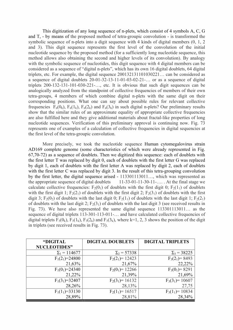
This digitization of any long sequence of n-plets, which consist of 4 symbols A, C, G and T, - by means of the proposed method of tetra-groupic convolution - is transformed the symbolic sequence of n-plets into a digit sequence with 4 kinds of digital members (0, 1, 2 and 3). This digit sequence represents the first level of the convolution of the initial nucleotide sequence by the proposed method (for a sufficiently long nucleotide sequence, this method allows also obtaining the second and higher levels of its convolution). By analogy with the symbolic sequence of nucleotides, this digit sequence with 4 digital members can be considered as a sequence of “digital n-plets”, which has its own 16 digital doublets, 64 digital triplets, etc. For example, the digital sequence 200132131101030221… can be considered as a sequence of digital doublets 20-01-32-13-11-01-03-02-21-… or as a sequence of digital triplets 200-132-131-101-030-221-…, etc. It is obvious that such digit sequences can be analogically analyzed from the standpoint of collective frequencies of members of their own tetra-groups, 4 members of which combine digital n-plets with the same digit on their corresponding positions. What one can say about possible rules for relevant collective frequencies Fn(0k), Fn(1k), Fn(2k) and Fn(3k) in such digital n-plets? Our preliminary results show that the similar rules of an approximate equality of appropriate collective frequencies are also fulfilled here and they give additional materials about fractal-like properties of long nucleotide sequences. Verification of this preliminary approval is continuing now. Fig. 73 represents one of examples of a calculation of collective frequencies in digital sequencies at the first level of the tetra-groupic convolution.

More precisely, we took the nucleotide sequence Human cytomegalovirus strain AD169 complete genome (some characteristics of which were already represented in Fig. 67,70-72) as a sequence of doublets. Then we digitized this sequence: each of doublets with the first letter T was replaced by digit 0, each of doublets with the first letter G was replaced by digit 1, each of doublets with the first letter A was replaced by digit 2, each of doublets with the first letter C was replaced by digit 3. In the result of this tetra-grouping convolution by the first letter, the digital sequence arised - 113301113011…, which was represented as the appropriate sequence of digital doublets 11-33-01-11-30-11-…. . At the final stage we calculate collective frequencies: F2(01) of doublets with the first digit 0; F2(11) of doublets with the first digit 1; F2(21) of doublets with the first digit 2; F2(31) of doublets with the first digit 3; F2(02) of doublets with the last digit 0; F2(11) of doublets with the last digit 1; F2(21) of doublets with the last digit 2; F2(31) of doublets with the last digit 3 (see received results in Fig. 73). We have also represented the same digital sequence 113301113011… as the sequence of digital triplets 113-301-113-011-… and have calculated collective frequencies of digital triplets F3(0k), F3(1k), F3(2k) and F3(3k), where k=1, 2, 3 shows the position of the digit in triplets (see received results in Fig. 73).

“DIGITAL NUCLEOTIDES”

DIGITAL DOUBLETS DIGITAL TRIPLETS

Σ1 = 114677 Σ2 = 57338 Σ3 = 38225 F1(21)=24800

21,63% F2(21)= 12423

21,67% F3(21)= 8493

22,22% F1(01)=24340

21,22% F2(01)= 12266

21,39% F3(01)= 8291

21,69% F1(31)=32407

28,26% F2(31)= 16132

28,13% F3(31)= 10607

27,75 F1(11)=33130

28,89% F2(11)= 16517

28,81% F3(11)= 10834

28,34%

Fig. 73. Collective frequencies F2(0k), F2(1k), F2(2k), F3(3k), F3(0k), F3(1k), F3(2k) and F3(3k) in the digital sequence, which arises in the result of the tetra-groupiс convolution of the sequence of doublets (by their first letter) of Human cytomegalovirus strain AD169 complete genome, 229354 bp, GenBank, accession X17403.1 (see explanation in text). The percentage of each of collective frequencies is also shown.

Fig. 73 shows that collective frequencies of digital doublets and triplets at the first level of this tetra-convolution are approximately in 2 time less than collective frequencies of doublets and tripples of the considered nucleotide sequence in Fig. 70.

Our work [Petoukhov, Svirin, 2012] has introduced the notion «fractal genetic nets» with a description of special transformations of long nucleotide sequencies. This transformations generate new shorter sequences of nucleotides, to study of which the proposed method of tetra-groupic equivalency of oligonucleotides is also applied.

In the end of this Section, one should say the following. The Chargaff's rules have plaid an important role in development of bioinformatics. We hope that the rules, which are described in this Section, will be also useful for further development of bioinformatics. In particular, these new rules testify in favor of usage of principles of logical holography and fractal compression of informatics in mathematical modeling of genetic structures and phenomena.

Our results reveal new hidden connections of long nucleotide sequences with fractal structures, which are associated with strange attractors of the chaotic dynamics. As known, fractals are to chaos what geometry is to algebra. They are the geometric manifestation of the chaotic dynamics. They are called "the fingerprints of chaos" sometimes. The revealing new hidden connections of long nucleotide sequences with fractals show additional possibilities of usage of ideology and mathematical tools of non-linear dynamics or chaotic dynamical systems in genetics. In particular, modern knowledge about so called chaotic communication systems and a special type of computers, which work on principles of chaotic dynamical systems [Dmitriev, 1998], can be apllied to understand genetic phenomena. In such approach,

F2(22)= 12377 21,59%

F3(22)= 8363 21,88%

F2(02)= 12074 21,06%

F3(02)= 8101 21,19%

F2(32)= 16275 28,38%

F3(32)= 10716 28,03%

F2(12)= 16612 28,97%

F3(12)= 11045 28,89%

F3(23)= 7943 20,78

F3(03)= 7948 20,79%

F3(33)= 11084 29,00%

F3(13)= 11250 29,43%

a living organism is represented as a set of chaotic dynamical computers and chaotic communication systems. This approach can be useful for progress in both - genetic and technological - fields. Taking into account our received results about the described rules (on the basis of tetra-groups of equivalency of oligonucleotide), we propose the new notion of genetic and epigenetic «tetra-codes». Also we should note two following thoughts connected with these tetra-codes:

• Genetic and epigenetic systems are collective essences and their secrets are connected with interactions of whole ensembles of genetic elements such as the described tetra-groups of oligonucleotides. Correspondingly, collective characteristics of genetic ensembles should be studied to reveal new secrets of genetic systems (by analogy with the described collective frequences of oligonucleotides on the basis of tetra-groups);

• The described quantitative rules reflect that the genetic coding systems in the whole use tetra-codes, which are digital representations of the described tetra-groups of oligonucleotides. In our opinion, these tetra-codes are useful for understanding the geno-logical coding [Petoukhov, Petukhova, 2017]. Study of these tetra-codes should use binary representations of oligonucleotides (in particular, decimal numbers 0, 1, 2 and 3 can be represented as members of the 2-bits dyadic group of binary numbers 00, 01, 10 and 11 on the basis of their biochemical binary-oppositional traits. To the theme of importance of tetra-groups and tetra-codes in genetics one can add

the fact of existence of 4 histones, which serve as the basis in the well known hypothetical histone code. In eukaryote cells, filaments of DNA are coiled around nucleosomes, each of which is a shank consisting of the histones of the four types: H2A, H2B, H3 and H4. This set of four types is divided by nature into the pairs of one-specific histones. The histones H2A and H2B possess the important possibility to create the pair just one with another on the basis of their mutual revealing and mutual “attraction”. Another pair consists of the histones H3 and H4, which possess the similar possibility to create the pairs just one with another on the analogical basis of their mutual revealing and mutual “attraction”. It is an interesting open question about a correspondence between the described tetra-groups of oligonucleotides and the tetra-group of histones in epigenetic coding properties of DNA. We think that epigenetic coding uses a set of interrelated tetra-codes of different nature.

SOME CONCLUDING REMARKS

As it was noted in the beginning of the article, living organism is a machine for coding and processing of information. For example, visual information about external objects is transmitted through the nerves from the eye retina to the brain already in a logarithmically encoded form. This article shows some evidences that oblique projection operators and their combinations, which are connected with matrix representations of the genetic coding system, can be a basis of adequate approaches to simulate ensembles of inherited biological phenomena. Only some of such phenomena were considered in this article. Some other phenomena will be described from the proposed point of view later. In addition, the author reminds about fractal genetic nets (FGN), which can be represented as a construction on a base of orthogonal projectors and which lead to new genetic rules in structures of long nucleotide sequences [Petoukhov, 2012; Petoukhov, Svirin, 2012].

The revealed genetic system of operators connected with oblique projectors allows modeling multi-dimensional phase spaces with many subspaces, processes in which can be selectively determined and controled. Speaking about importance of projectors in the nature, the following points should be noted (it seems that the nature «likes» projectors):

• Most people are familiar with the idea of projectors due to sun rays (and light rays in general) that are distributed in a straight line and provide shade from the subjects (from the ancient time sundials were constructed on the use of this). Light rays have the projection property;

• Electromagnetic vectors are the sum of their projections in the form of their electric and magnetic vectors;

• Evolution of living organisms is associated with the consumption of solar energy that is projected by means of sun rays to surfaces of living bodies (photosynthesis, which is for living matter one of its basic mechanisms, is the conversion of sunlight energy into biochemical energy for activity of organisms; circadian biorhythms are connected with external light cycles "day-night");

• Projection phenomena of birefringence in biological tissues and crystals exist; • A great variety of living organisms has polarization eyesight; • Our vision is based on the projection of images on the retina; • Religious people may ask whether there is any indication in the Bible on this subject?

Especially for them, it may be recalled the following. According to the Bible, God's creation of the world began with the creation of the light: "Let there be light." Many thinkers suggested previously for various reasons that, figuratively speaking, the body is woven from the light. This has some associations with our hypothesis that the body is woven from the projectors.

Now projectors and their combinations become interesting instruments to study and simulate genetic phenomena and inherited structures and processes in living matter. A new conceptual notion with appropriate mathematical formalisms are proposed about a multi-dimensional control space (or coding space) with subspaces of a selective control in each on basis of a participation of projection operators in such control. Here one can remember the statement: “Profound study of nature is the most fertile source of mathematical discoveries” (Fourier, 2006, Chapter 1, p. 7).

Using this ideology of projection operators, one can get many unexpected results and approaches. In author's opinion, one of many promising applications of projectors in mathematical biology and bioinformatics is the study of connections between genetic projectors and Boolean algebra. It is known that every family of commutative projectors generates a Boolean algebra of projectors. The Boolean algebra plays a great role in the modern science because of its connections with many scientific branches: mathematical logic, the problem of artificial intelligence, computer technologies, bases of theory of probability, etc. G.Boole was creating such algebra of logics (or logical operators), which would reflect inherited laws of human thought. One should note here that some of genetic projectors (which are not described in this article) form commutative pairs; this fact provokes thoughts about Boolean algebras in genetics and bioinformatics and also about genetic basis of logics of human thought. The connection of Boolean algebra with commutative projectors is essential also for development of our concept of geno-lohical coding [Petoukhov, 2016 ; Petoukhov, Petukhova, 2017].

Genetic molecules are subordinated to laws of quantum mechanics, which has begun from matrix mechanics by W. Heisenberg. Till this pioneer work by Heisenberg, matrices were not used in physics. It was very unexpected for scientific community that applying whole ensembles of numbers in a form of matrices can be useful and appropriate to describe natural phenomena and systems. Contemporary science uses matrices widely in many fields, and our work uses matrices to study molecular-genetic systems.

Materials of this article reinforce the author’s point of view that living matter in its informational fundamentals is an algebraic essence. The author believes that a development of algebraic biology, elements of which are contained in this and other author’s articles, is possible. By analogy with the known fact that molecular foundations of molecular genetics turned up unexpectedly very simple, perhaps algebraic foundations of living matter are also relative simple. In the infinite set of matrices, we find a small subset, which simulates the world of molecular genetic coding with many of its phenomenologic features; this discovery was possible due to studying the family of alphabets in the molecular-genetic system. The matrix-algebraic approach to structured genetic alphabets has led the author, in particular, to the rules of long nucleotide sequences, which are described and discussed in the Section 17.

The new theme of systems of 2n-block united-hypercomplex numbers (U-hypercomplex numbers), which are new mathematical tools for modeling different structures, was included in the 7th and 8th versions of this article (see Sections 15 and 16). These numeric systems generalize systems of complex numbers and hypercomplex numbers, which become a particular case of appropriate systems of 2n-block united-hypercomplex numbers when only one block in them differs from zero. Hypercomplex numbers, beginning from quaternions of Hamilton, were created as an extension of complex numbers by means of including new independent imaginary units in addition to a single imaginary unit of complex numbers. In our studies of genetic matrices we paid attention on the alternative way of extention of complex numbers: such extension is provided by means of including new independent real units (one or more real units, which we call local-real units) together with their particular complect of imaginary units (local-imaginary units). The world of sparse matrices gives a comfortable possibility of the creation of such U-hypercomplex numbers.

One can remind that the idea of multi-dimensional numbers and multi-dimensional spaces works intensively for a long time in theoretical physics and other fields of science for modeling the phenomena of our physical world. Our results add mathematical formalisms, first of all, into the fields of molecular genetics and bioinformatics. After the discovery of non-Euclidean geometries and of Hamilton quaternions, it is known that different natural systems can possess their own geometry and their own algebra (see about this [Kline, 1980]).

But what kinds of algebra are appropriate for living organisms in their bioinformational aspects? We believe that the algebraic organization of any of living organisms in its inherited bioinformational aspects is based (or can be modelled) on systems of 2n-block U-hypercomplex numbers. It seems that many difficulties of modern bioinformatics and mathematical biology are connected with utilizing - for biological structures - inadequate algebras, which were developed for completely other natural systems. Hamilton had similar difficulties in his attempts to describe transformations in a three-dimensional space by means of 3-dimensional numbers while this description needs 4-parametrical quaternions. The author simultaneously hopes that the proposed U-hypercomplex numbers will help to make progress not only in bioinformatics and mathematical biology, where algebraization of biology is under development now, but also in many fields of sciences and technologies. In physics, these U-hypercomplex numbers can lead to new unexpected concepts and theories by generalizing or combining existing concepts and theories. For example, the following question arises: is it possible to connect - in modelling aims - the "wave-particle" duality of quantum-mechanical objects (which are manifested in different measurement experiments or as a particle, or as a wave) with 2-block U-numbers, in which both blocks are mutually related, but in different experiments only one of two blocks manifests itself in its projection onto a measuring device? In other words, for quantum-mechanical objects in this approach different physical experiments manifest characteristics of different blocks of the same 2-block U-number.

Multiblock structure, which is genetically inherited, is one of the most characteristic features of a plurality of living bodies on different levels and branches of biological evolution. The author believes that systems of multiblock U-hypercomplex numbers represent a relevant mathematics for modeling such inherited structures. But non-living substances also consist of various blocks of different levels up to atoms atoms and elementary particles (one of the most important statements in the history of science has been done by Democritus approximately in the fourth century BC: "All bodies are composed of discrete units - atoms"). It is not excluded that the proposed systems of multiblock U-hypercomplex numbers will be also useful in theoretical physics to study block structure of substances.

“Complexity of a civilization is reflected in complexity of numbers used by this civilization” [Davis, 1967]. Pythagoras has formulated the idea: “all things in the world are numbers” or “number rules the world”. B. Russell noted that he did not know other person who would exert such influence on thinking of people as Pythagoras. From this viewpoint, there is no more fundamental scientific idea in the world, than this idea about a basic meaning of numbers. Our researches in the field of matrix genetics have led to new systems of multidimensional numbers and have given new materials to the great idea by Pythagoras in its modernized formulating: “All things are multi-dimensional numbers”.

This article proposes a new mathematical approach to study “a partnership between genes and mathematics” (see Section 1 above). In the author’s opinion, the proposed kind of mathematics is beautiful and it can be used for further developing of algebraic biology, theoretical physics and informatics in accordance with the famous statement by P. Dirac, who taught that a creation of a physical theory must begin with the beautiful mathematical theory: “If this theory is really beautiful, then it necessarily will appear as a fine model of important physical phenomena. It is necessary to search for these phenomena to develop applications of the beautiful mathematical theory and to interpret them as predictions of new laws of physics” (this quotation is taken from [Arnold, 2007]). According to Dirac, all new physics, including relativistic and quantum, are developing in this way. One can suppose that this statement is also true for mathematical biology.

APPENDIX 1. COMPLEX NUMBERS, CYCLIC GROUPS AND SUMS OF

GENETIC PROJECTORS This Appendix shows a connection between complex numbers and cyclic groups on

the base of sums of (8*8)-projectors s0+s2, s0+s3, s1+s2, s1+s3, s4+s6, s4+s7, s5+s6, s5+s7 from Fig. 7 on the base of the Rademacher (8*8)-matrix R8 (on Fig. 9 these sums were marked by green color and they corresponded to cyclic groups, if the weight coefficient 2-0.5 was used for them). Each of these 8 sums can be decomposed into two matrices e2k and e2k+1 (k=0, 1, …7), a set of whose is closed relative to multiplication and has a multiplication table, which coincides with the multiplication table of basic elements of complex numbers (Fig. 74). It means that these matrices e2k and e2k+1 represent basic elements of complex numbers in corresponding 2-dimensional planes of a 8-dimensional vector space. Sets of matrices a2k*e2k + a2k+1*e2k+1 (here a2k and a2k+1 are real numbers; each of matrices e2k plays a role of unitary matrix inside the appropriate set a2k*e2k + a2k+1*e2k+1) represent complex numbers inside these 2-dimensional planes of the 8-dimensional space.

s0+s2 =

1 0 1 0 0 0 0 0 1 0 1 0 0 0 0 0 -1 0 1 0 0 0 0 0 -1 0 1 0 0 0 0 0 1 0-1 0 0 0 0 0 1 0-1 0 0 0 0 0 -1 0-1 0 0 0 0 0 -1 0-1 0 0 0 0 0

=e0+e1=

1 0 0 0 0 0 0 0 1 0 0 0 0 0 0 0 0 0 1 0 0 0 0 0 0 0 1 0 0 0 0 0 0 0 -1 0 0 0 0 0 0 0 -1 0 0 0 0 0 -1 0 0 0 0 0 0 0 -1 0 0 0 0 0 0 0

+

0 0 1 0 0 0 0 0 0 0 1 0 0 0 0 0 -1 0 0 0 0 0 0 0 -1 0 0 0 0 0 0 0 1 0 0 0 0 0 0 0 1 0 0 0 0 0 0 0 0 0-1 0 0 0 0 0 0 0-1 0 0 0 0 0

;

e0 e1

e0 e0 e1

e1 e1 -e0

s0+s3 =

1 0 0 1 0 0 0 0 1 0 0 1 0 0 0 0 -1 0 0 1 0 0 0 0 -1 0 0 1 0 0 0 0 1 0 0 -1 0 0 0 0 1 0 0 -1 0 0 0 0 -1 0 0 -1 0 0 0 0 -1 0 0 -1 0 0 0 0

=e2+e3=

1 0 0 0 0 0 0 0 1 0 0 0 0 0 0 0 0 0 0 1 0 0 0 0 0 0 0 1 0 0 0 0 0 0 0 -1 0 0 0 0 0 0 0 -1 0 0 0 0 -1 0 0 0 0 0 0 0 -1 0 0 0 0 0 0 0

+

0 0 0 1 0 0 0 0 0 0 0 1 0 0 0 0 -1 0 0 0 0 0 0 0 -1 0 0 0 0 0 0 0 1 0 0 0 0 0 0 0 1 0 0 0 0 0 0 0 0 0 0-1 0 0 0 0 0 0 0-1 0 0 0 0

;

e2 e3

e2 e2 e3

e3 e3 -e2

s1+s2 =

0 1 1 0 0 0 0 0 0 1 1 0 0 0 0 0 0 -1 1 0 0 0 0 0 0 -1 1 0 0 0 0 0 0 1 -1 0 0 0 0 0 0 1 -1 0 0 0 0 0 0 -1 -1 0 0 0 0 0 0 -1 -1 0 0 0 0 0

=e4+e5=

0 1 0 0 0 0 0 0 0 1 0 0 0 0 0 0 0 0 1 0 0 0 0 0 0 0 1 0 0 0 0 0 0 0 -1 0 0 0 0 0 0 0 -1 0 0 0 0 0 0 -1 0 0 0 0 0 0 0 -1 0 0 0 0 0 0

+

0 0 1 0 0 0 0 0 0 0 1 0 0 0 0 0 0 -1 0 0 0 0 0 0 0 -1 0 0 0 0 0 0 0 1 0 0 0 0 0 0 0 1 0 0 0 0 0 0 0 0 -1 0 0 0 0 0 0 0 -1 0 0 0 0 0

;

e4 e5

e4 e4 e5

e5 e5 -e4

s1+s3 =

0 1 0 1 0 0 0 0 0 1 0 1 0 0 0 0 0-1 0 1 0 0 0 0 0-1 0 1 0 0 0 0 0 1 0-1 0 0 0 0 0 1 0-1 0 0 0 0 0-1 0-1 0 0 0 0 0-1 0-1 0 0 0 0

=e6+e7=

0 1 0 0 0 0 0 0 0 1 0 0 0 0 0 0 0 0 0 1 0 0 0 0 0 0 0 1 0 0 0 0 0 0 0-1 0 0 0 0 0 0 0-1 0 0 0 0 0-1 0 0 0 0 0 0 0-1 0 0 0 0 0 0

+

0 0 0 1 0 0 0 0 0 0 0 1 0 0 0 0 0-1 0 0 0 0 0 0 0-1 0 0 0 0 0 0 0 1 0 0 0 0 0 0 0 1 0 0 0 0 0 0 0 0 0-1 0 0 0 0 0 0 0-1 0 0 0 0

;

e6 e7

e6 e6 e7

e7 e7 -e6

s4+s6 =

0 0 0 0 1 0-1 0 0 0 0 0 1 0-1 0 0 0 0 0-1 0-1 0 0 0 0 0-1 0-1 0 0 0 0 0 1 0 1 0 0 0 0 0 1 0 1 0 0 0 0 0-1 0 1 0 0 0 0 0-1 0 1 0

=e8+e9=

0 0 0 0 0 0-1 0 0 0 0 0 0 0-1 0 0 0 0 0-1 0 0 0 0 0 0 0-1 0 0 0 0 0 0 0 1 0 0 0 0 0 0 0 1 0 0 0 0 0 0 0 0 0 1 0 0 0 0 0 0 0 1 0

+

0 0 0 0 1 0 0 0 0 0 0 0 1 0 0 0 0 0 0 0 0 0-1 0 0 0 0 0 0 0-1 0 0 0 0 0 0 0 1 0 0 0 0 0 0 0 1 0 0 0 0 0-1 0 0 0 0 0 0 0-1 0 0 0

;

e8 e9

e8 e8 e9

e9 e9 -e8

s4+s7 =

0 0 0 0 1 0 0-1 0 0 0 0 1 0 0-1 0 0 0 0-1 0 0-1 0 0 0 0-1 0 0-1 0 0 0 0 1 0 0 1 0 0 0 0 1 0 0 1 0 0 0 0-1 0 0 1 0 0 0 0-1 0 0 1

=e10+e11=

0 0 0 0 0 0 0-1 0 0 0 0 0 0 0-1 0 0 0 0-1 0 0 0 0 0 0 0-1 0 0 0 0 0 0 0 1 0 0 0 0 0 0 0 1 0 0 0 0 0 0 0 0 0 0 1 0 0 0 0 0 0 0 1

+

0 0 0 0 1 0 0 0 0 0 0 0 1 0 0 0 0 0 0 0 0 0 0 -1 0 0 0 0 0 0 0 -1 0 0 0 0 0 0 0 1 0 0 0 0 0 0 0 1 0 0 0 0-1 0 0 0 0 0 0 0-1 0 0 0

;

e10 e11

e10 e10 e11

e11 e11 -e10

s5+s6 =

0 0 0 0 0 1 -1 0 0 0 0 0 0 1 -1 0 0 0 0 0 0 -1 -1 0 0 0 0 0 0 -1 -1 0 0 0 0 0 0 1 1 0 0 0 0 0 0 1 1 0 0 0 0 0 0 -1 1 0 0 0 0 0 0 -1 1 0

=e12+e13=

0 0 0 0 0 0 -1 0 0 0 0 0 0 0 -1 0 0 0 0 0 0 -1 0 0 0 0 0 0 0 -1 0 0 0 0 0 0 0 1 0 0 0 0 0 0 0 1 0 0 0 0 0 0 0 0 1 0 0 0 0 0 0 0 1 0

+

0 0 0 0 0 1 0 0 0 0 0 0 0 1 0 0 0 0 0 0 0 0 -1 0 0 0 0 0 0 0 -1 0 0 0 0 0 0 0 1 0 0 0 0 0 0 0 1 0 0 0 0 0 0 -1 0 0 0 0 0 0 0 -1 0 0

;

e12 e13

e12 e12 e13

e13 e13 -e12

s5+s7 =

0 0 0 0 0 1 0 -1 0 0 0 0 0 1 0 -1 0 0 0 0 0 -1 0 -1 0 0 0 0 0 -1 0 -1 0 0 0 0 0 1 0 1 0 0 0 0 0 1 0 1 0 0 0 0 0 -1 0 1 0 0 0 0 0 -1 0 1

=e14+e15=

0 0 0 0 0 0 0 -1 0 0 0 0 0 0 0 -1 0 0 0 0 0 -1 0 0 0 0 0 0 0 -1 0 0 0 0 0 0 0 1 0 0 0 0 0 0 0 1 0 0 0 0 0 0 0 0 0 1 0 0 0 0 0 0 0 1

+

0 0 0 0 0 1 0 0 0 0 0 0 0 1 0 0 0 0 0 0 0 0 0 -1 0 0 0 0 0 0 0 -1 0 0 0 0 0 0 0 1 0 0 0 0 0 0 0 1 0 0 0 0 0 -1 0 0 0 0 0 0 0 -1 0 0

;

e14 e15

e14 e14 e15

e15 e15 -e14

Fig. 74. The decomposition of each of (8*8)-matrices s0+s2, s0+s3, s1+s2, s1+s3, s4+s6,

s4+s7, s5+s6, s5+s7 from Fig. 7 into a set of two matrices e2k and e2k+1 (k=0, 1, …7), a set of whose is closed relative to multiplication and gives the multiplication table of complex numbers (on the right)

In a general case, the described approach allows constructing selective operators of a 2n-dimensional vector space with a set of different 2-dimensional planes, each of which can contain a function of complex numbers (parameters of these functions in different planes can be independent or interrelated). Such selective operator allows simulating a combinatory behaviour of a multi-parametric system, which contains different 2-parametric subsystems, whose independent or interrelated behaviours can be simulated by means of functions of complex numbers. If these functions of complex numbers are cyclic, such selective operator describes a behaviour of a multi-parametric system, which contains an appropriate ensemble of 2-parametric subsystems with cyclic behaviours.

APPENDIX 2. HYPERBOLIC NUMBERS AND SUMS OF GENETIC PROJECTORS

Let us show now a connection between hyperbolic numbers and sums of (8*8)-projectors s0+s1, s0+s4, s0+s5, s1+s4, s1+s5, s2+s3, s2+s6, s2+s7, s3+s6, s3+s7, s4+s5, s6+s7 from Fig. 7 on the base of the Rademacher (8*8)-matrix R8 (on Fig. 9 these sums were marked by red color). Each of these 12 sums can be decomposed into two matrices j2k and j2k+1 (k=0, 1, 2, …, 11), a set of whose is closed relative to multiplication and has a multiplication table, which coincides with the multiplication table of basic elements of hyperbolic numbers (Fig. 75). It means that these matrices j2k and j2k+1 represent basic elements of hyperbolic numbers in corresponding 2-dimensional planes of a 8-dimensional vector space. Sets of matrices a2k*j2k + a2k+1*j2k+1 (here a2k and a2k+1 are real numbers; each of matrices j2k plays a role of unitary matrix inside the appropriate set a2k*j2k + a2k+1*j2k+1) represent hyperbolic numbers inside these 2-dimensional planes of the 8-dimensional space.

s0+s1 =

1 1 0 0 0 0 0 0 1 1 0 0 0 0 0 0 -1 -1 0 0 0 0 0 0 -1 -1 0 0 0 0 0 0 1 1 0 0 0 0 0 0 1 1 0 0 0 0 0 0 -1 -1 0 0 0 0 0 0 -1 -1 0 0 0 0 0 0

= j0+j1=

1 0 0 0 0 0 0 0 0 1 0 0 0 0 0 0 -1 0 0 0 0 0 0 0 0 -1 0 0 0 0 0 0 1 0 0 0 0 0 0 0 0 1 0 0 0 0 0 0 -1 0 0 0 0 0 0 0 0 -1 0 0 0 0 0 0

+

0 1 0 0 0 0 0 0 1 0 0 0 0 0 0 0 0 -1 0 0 0 0 0 0 -1 0 0 0 0 0 0 0 0 1 0 0 0 0 0 0 1 0 0 0 0 0 0 0 0 -1 0 0 0 0 0 0 -1 0 0 0 0 0 0 0

;

j0 j1

j0 j0 j1

j1 j1 j0

s0+s4 =

1 0 0 0 1 0 0 0 1 0 0 0 1 0 0 0 -1 0 0 0 -1 0 0 0 -1 0 0 0 -1 0 0 0 1 0 0 0 1 0 0 0 1 0 0 0 1 0 0 0 -1 0 0 0 -1 0 0 0 -1 0 0 0 -1 0 0 0

= j2+j3=

1 0 0 0 0 0 0 0 1 0 0 0 0 0 0 0 0 0 0 0 -1 0 0 0 0 0 0 0 -1 0 0 0 0 0 0 0 1 0 0 0 0 0 0 0 1 0 0 0 -1 0 0 0 0 0 0 0 -1 0 0 0 0 0 0 0

+

0 0 0 0 1 0 0 0 0 0 0 0 1 0 0 0 -1 0 0 0 0 0 0 0 -1 0 0 0 0 0 0 0 1 0 0 0 0 0 0 0 1 0 0 0 0 0 0 0 0 0 0 0 -1 0 0 0 0 0 0 0 -1 0 0 0

;

j2 j3

j2 j2 j3

j3 j3 j2

s0+s5 =

1 0 0 0 0 1 0 0 1 0 0 0 0 1 0 0 -1 0 0 0 0 -1 0 0 -1 0 0 0 0 -1 0 0 1 0 0 0 0 1 0 0 1 0 0 0 0 1 0 0 -1 0 0 0 0 -1 0 0 -1 0 0 0 0 -1 0 0

=j4+j5=

1 0 0 0 0 0 0 0 1 0 0 0 0 0 0 0 0 0 0 0 0-1 0 0 0 0 0 0 0-1 0 0 0 0 0 0 0 1 0 0 0 0 0 0 0 1 0 0 -1 0 0 0 0 0 0 0 -1 0 0 0 0 0 0 0

+

0 0 0 0 0 1 0 0 0 0 0 0 0 1 0 0 -1 0 0 0 0 0 0 0 -1 0 0 0 0 0 0 0 1 0 0 0 0 0 0 0 1 0 0 0 0 0 0 0 0 0 0 0 0 -1 0 0 0 0 0 0 0 -1 0 0

;

j4 j5

j4 j4 j5

j5 j5 j4

s1+s4 =

0 1 0 0 1 0 0 0 0 1 0 0 1 0 0 0 0 -1 0 0 -1 0 0 0 0 -1 0 0 -1 0 0 0

= j6+j7=

0 1 0 0 0 0 0 0 0 1 0 0 0 0 0 0 0 0 0 0-1 0 0 0 0 0 0 0-1 0 0 0

+

0 0 0 0 1 0 0 0 0 0 0 0 1 0 0 0 0 -1 0 0 0 0 0 0 0 -1 0 0 0 0 0 0

;

j6 j7

0 1 0 0 1 0 0 0 0 1 0 0 1 0 0 0 0 -1 0 0 -1 0 0 0 0 -1 0 0 -1 0 0 0

0 0 0 0 1 0 0 0 0 0 0 0 1 0 0 0 0 -1 0 0 0 0 0 0 0 -1 0 0 0 0 0 0

0 1 0 0 0 0 0 0 0 1 0 0 0 0 0 0 0 0 0 0 -1 0 0 0 0 0 0 0 -1 0 0 0

j6 j6 j7

j7 j7 j6

s1+s5 =

0 1 0 0 0 1 0 0 0 1 0 0 0 1 0 0 0 -1 0 0 0 -1 0 0 0 -1 0 0 0 -1 0 0 0 1 0 0 0 1 0 0 0 1 0 0 0 1 0 0 0 -1 0 0 0 -1 0 0 0 -1 0 0 0 -1 0 0

= j8+j9=

0 1 0 0 0 0 0 0 0 1 0 0 0 0 0 0 0 0 0 0 0 -1 0 0 0 0 0 0 0 -1 0 0 0 0 0 0 0 1 0 0 0 0 0 0 0 1 0 0 0-1 0 0 0 0 0 0 0-1 0 0 0 0 0 0

+

0 0 0 0 0 1 0 0 0 0 0 0 0 1 0 0 0 -1 0 0 0 0 0 0 0 -1 0 0 0 0 0 0 0 1 0 0 0 0 0 0 0 1 0 0 0 0 0 0 0 0 0 0 0 -1 0 0 0 0 0 0 0 -1 0 0

;

j8 j9

j8 j8 j9

j9 j9 j8

s2+s3=

0 0 1 1 0 0 0 0 0 0 1 1 0 0 0 0 0 0 1 1 0 0 0 0 0 0 1 1 0 0 0 0 0 0 -1-1 0 0 0 0 0 0 -1-1 0 0 0 0 0 0 -1-1 0 0 0 0 0 0 -1-1 0 0 0 0

= j10+j11=

0 0 1 0 0 0 0 0 0 0 0 1 0 0 0 0 0 0 1 0 0 0 0 0 0 0 0 1 0 0 0 0 0 0 -1 0 0 0 0 0 0 0 0 -1 0 0 0 0 0 0 -1 0 0 0 0 0 0 0 0 -1 0 0 0 0

+

0 0 0 1 0 0 0 0 0 0 1 0 0 0 0 0 0 0 0 1 0 0 0 0 0 0 1 0 0 0 0 0 0 0 0 -1 0 0 0 0 0 0 -1 0 0 0 0 0 0 0 0 -1 0 0 0 0 0 0 -1 0 0 0 0 0

;

j10 j11

j10 j10 j11

j11 j11 j10

s2+s6 =

0 0 1 0 0 0 -1 0 0 0 1 0 0 0 -1 0 0 0 1 0 0 0 -1 0 0 0 1 0 0 0 -1 0 0 0 -1 0 0 0 1 0 0 0 -1 0 0 0 1 0 0 0 -1 0 0 0 1 0 0 0 -1 0 0 0 1 0

=j12+j13=

0 0 1 0 0 0 0 0 0 0 1 0 0 0 0 0 0 0 0 0 0 0 -1 0 0 0 0 0 0 0 -1 0 0 0 0 0 0 0 1 0 0 0 0 0 0 0 1 0 0 0 -1 0 0 0 0 0 0 0 -1 0 0 0 0 0

+

0 0 0 0 0 0-1 0 0 0 0 0 0 0-1 0 0 0 1 0 0 0 0 0 0 0 1 0 0 0 0 0 0 0-1 0 0 0 0 0 0 0-1 0 0 0 0 0 0 0 0 0 0 0 1 0 0 0 0 0 0 0 1 0

;

j12 j13

j12 j12 j13

j13 j13 j12

s2+s7 =

0 0 1 0 0 0 0 -1 0 0 1 0 0 0 0 -1 0 0 1 0 0 0 0 -1 0 0 1 0 0 0 0 -1 0 0 -1 0 0 0 0 1 0 0 -1 0 0 0 0 1 0 0 -1 0 0 0 0 1 0 0 -1 0 0 0 0 1

=j14+j15=

0 0 1 0 0 0 0 0 0 0 1 0 0 0 0 0 0 0 0 0 0 0 0 -1 0 0 0 0 0 0 0 -1 0 0 0 0 0 0 0 1 0 0 0 0 0 0 0 1 0 0 -1 0 0 0 0 0 0 0 -1 0 0 0 0 0

+

0 0 0 0 0 0 0 -1 0 0 0 0 0 0 0 -1 0 0 1 0 0 0 0 0 0 0 1 0 0 0 0 0 0 0 -1 0 0 0 0 0 0 0 -1 0 0 0 0 0 0 0 0 0 0 0 0 1 0 0 0 0 0 0 0 1

;

j14 j15

j14 j14 j15

j15 j15 j14

s3+s6 =

0 0 0 1 0 0 -1 0 0 0 0 1 0 0 -1 0 0 0 0 1 0 0 -1 0 0 0 0 1 0 0 -1 0

=j16+j17=

0 0 0 1 0 0 0 0 0 0 0 1 0 0 0 0 0 0 0 0 0 0 -1 0 0 0 0 0 0 0 -1 0

+

0 0 0 0 0 0 -1 0 0 0 0 0 0 0 -1 0 0 0 0 1 0 0 0 0 0 0 0 1 0 0 0 0

;

j16 j17

0 0 0 -1 0 0 1 0 0 0 0 -1 0 0 1 0 0 0 0 -1 0 0 1 0 0 0 0 -1 0 0 1 0

0 0 0 0 0 0 1 0 0 0 0 0 0 0 1 0 0 0 0 -1 0 0 0 0 0 0 0 -1 0 0 0 0

0 0 0 -1 0 0 0 0 0 0 0 -1 0 0 0 0 0 0 0 0 0 0 1 0 0 0 0 0 0 0 1 0

j16 j16 j17

j17 j17 j16

s3+s7 =

0 0 0 1 0 0 0 -1 0 0 0 1 0 0 0 -1 0 0 0 1 0 0 0 -1 0 0 0 1 0 0 0 -1 0 0 0 -1 0 0 0 1 0 0 0 -1 0 0 0 1 0 0 0 -1 0 0 0 1 0 0 0 -1 0 0 0 1

=j18+j19=

0 0 0 1 0 0 0 0 0 0 0 1 0 0 0 0 0 0 0 0 0 0 0 -1 0 0 0 0 0 0 0 -1 0 0 0 0 0 0 0 1 0 0 0 0 0 0 0 1 0 0 0 -1 0 0 0 0 0 0 0 -1 0 0 0 0

+

0 0 0 0 0 0 0 -1 0 0 0 0 0 0 0 -1 0 0 0 1 0 0 0 0 0 0 0 1 0 0 0 0 0 0 0-1 0 0 0 0 0 0 0-1 0 0 0 0 0 0 0 0 0 0 0 1 0 0 0 0 0 0 0 1

;

j18 j19

j18 j18 j19

j19 j19 j18

s4+s5 =

0 0 0 0 1 1 0 0 0 0 0 0 1 1 0 0 0 0 0 0 -1 -1 0 0 0 0 0 0 -1 -1 0 0 0 0 0 0 1 1 0 0 0 0 0 0 1 1 0 0 0 0 0 0 -1 -1 0 0 0 0 0 0 -1 -1 0 0

=j20+j21=

0 0 0 0 1 0 0 0 0 0 0 0 0 1 0 0 0 0 0 0-1 0 0 0 0 0 0 0 0-1 0 0 0 0 0 0 1 0 0 0 0 0 0 0 0 1 0 0 0 0 0 0-1 0 0 0 0 0 0 0 0-1 0 0

+

0 0 0 0 0 1 0 0 0 0 0 0 1 0 0 0 0 0 0 0 0-1 0 0 0 0 0 0-1 0 0 0 0 0 0 0 0 1 0 0 0 0 0 0 1 0 0 0 0 0 0 0 0-1 0 0 0 0 0 0-1 0 0 0

;

j20 j21

j20 j20 j21

j21 j21 j20

s6+s7 =

0 0 0 0 0 0 -1 -1 0 0 0 0 0 0 -1 -1 0 0 0 0 0 0 -1 -1 0 0 0 0 0 0 -1 -1 0 0 0 0 0 0 1 1 0 0 0 0 0 0 1 1 0 0 0 0 0 0 1 1 0 0 0 0 0 0 1 1

=j22+j23=

0 0 0 0 0 0 -1 0 0 0 0 0 0 0 0 -1 0 0 0 0 0 0 -1 0 0 0 0 0 0 0 0 -1 0 0 0 0 0 0 1 0 0 0 0 0 0 0 0 1 0 0 0 0 0 0 1 0 0 0 0 0 0 0 0 1

+

0 0 0 0 0 0 0 -1 0 0 0 0 0 0 -1 0 0 0 0 0 0 0 0 -1 0 0 0 0 0 0 -1 0 0 0 0 0 0 0 0 1 0 0 0 0 0 0 1 0 0 0 0 0 0 0 0 1 0 0 0 0 0 0 1 0

;

j22 j23

j22 j22 j23

j23 j23 j22

Fig. 75. The decomposition of each of (8*8)-matrices s0+s1, s0+s4, s0+s5, s1+s4, s1+s5,

s2+s3, s2+s6, s2+s7, s3+s6, s3+s7, s4+s5, s6+s7 from Fig. 7 into a set of two matrices j2k and j2k+1 (k=0, 1, …, 11), a set of whose is closed relative to multiplication and gives the multiplication table of hyperbolic numbers (on the right)

APPENDIX 3. ANOTHER TENSOR FAMILY OF GENETIC HADAMARD MATRICES

Hadamard matrices are well-‐known in noise-‐immunity coding, quantum mechanics, etc. Their rows are Walsh functions, which are widely used in radiocommunication for a code division in systems with many channels, etc., for example, in cellular standards such as IS-‐95, CDMA2000 or UMTS. Walsh functions and corresponding series and transforms find various applications in physics and engineereing, in particular, in digital signal processing. They are used in speech

recognition, in medical and biological image processing, in digital holography, and other areas.

Above we have described the variant of the relation of the molecular-genetic system with the special tensor family of Hadamard matrices H4, H8, etc. (Fig. 1 and 38). This variant uses the phenomenological fact of existence of triplets with strong and weak roots; in other words this variant is based on a specifity of the degeneracy of the genetic code. This Appendix shows second variant of a relation of the genetic alphabets with another tensor family of Hadamard matrices. This new family of genetic Hadamard matrices is based only on properties of the genetic alphabet A, C, G, T and doesn't depend on the degeneracy of the genetic code. On the author's opinion, this new variant is more interesting and fundamental for further using in future genetic researches.

Fig. 76 shows the beginning of this new tensor family of Hadamard matrices P(n) = [1 1; -1 1](n) together with genetic matrices [C T; A G](m) (m=1, 2, 3) of monoplets, duplets and triplets with their black-and-white mosaics which coincide with mosaics of the Hadamard matrices.

P2 =

; P8 =

1 -1 -1 1 -1 1 1 -1 1 1 -1 -1 -1 -1 1 1

; P4 =

1 -1 -1 1 1 -1 1 -1 -1 1 -1 1 1 -1 1 1 -1 -1 1 1 1 1 -1 -1 -1 -1 1 1 1 -1 1 -1 1 -1 -1 1 1 -1 -1 1

1 1 1 1 1 1 -1 -1 1 1 -1 -1 1 -1 1 -1 1 -1 1 -1

1 1 1 1 1 1 1 1

;

CCC CCT CTC CTT TCC TCT TTC TTT CCA CCG CTA CTG TCA TCG TTA TTG

;

CC CT TC TT CAC CAT CGC CGT TAC TAT TGC TGT C T CA CG TA TG CAA CAG CGA CGG TAA TAG TGA TGG A G AC AT GC GT ACC ACT ATC ATT GCC GCT GTC GTT

AA AG GA GG ACA ACG ATA ATG GCA GCG GTA GTG

AAC AAT AGC AGT GAC GAT GGC GGT AAA AAG AGA AGG GAA GAG GGA GGG

Fig. 76. Upper level: the beginning of the tensor family of Hadamard matrices P(n) =

[1 1; -1 1](n), where P4 = [1 1; -1 1](2) and P8 = [1 1; -1 1](3). Bottom level: genetic matrices [C T; A G], [C T; A G](2) and [C T; A G](3) of monoplets, duplets and triplets with their black-and-white mosaics, which coincide with mosaics of the Hadamard matrices P2, P4, P8.

On Fig. 76 the black-and-white matrices P2, P4, P8 are Hadamard matrices because

they satisfy the criterium Hn*HnT=n*E [Ahmed, Rao,1975]. The genetic matriices

[C T; A G], [C T; A G](2) and [C T; A G](3) algorithmically have the same black-and-white mosaics on the base of fundamental properties of the DNA alphabet (adenine A, cytosine C, guanine G and thymine T). These properties contrapose the letter T against three other letters of the DNA-alphabet by the following phenomenological facts:

• the thymine T is a single nitrogenous base in DNA which is replaced in RNA by another nitrogenous base U (uracil) for unknown reason;

• the thymine T is a single nitrogenous base in DNA without the amino-group NH2 (Fig. 77), which plays an important role in molecular genetics. For instance, the amino-group in amino acids provides a function of recognition of the amino acids by ferments [Chapeville, Haenni, 1974]. A detachment of amino-groups in nitrogenous bases A and C in RNA under action of nitrous acid HNO2 determines a property of amino-mutating of these bases, which was used to divide the set of 64 triplets into eight natural subsets with 8 triplets in each [Wittmann, 1961].

Fig. 77. The complementary pairs of the four nitrogenous bases in DNA. A-T (adenine and thymine), C-G (cytosine and guanine). Amino-groups NH2 are marked by big circles. Black circles are atoms of carbon; small white circles are atoms of hydrogen; squares with the letter N are atoms of nitrogen; triangles with the letter O are atoms of oxygen.

From the point of view of these two facts, the letters A, C, G are identical to each other and the letter T is opposite to them. Correspondingly this binary-oppositional division inside the DNA-alphabet can be reflected by the symbol “+1” for each of the letters A, C, G and by the opposite symbol “-1” for the letter T. Concerning the genetic matrices [C T; A G](n) this approach leads to a simple algorithm for assigning a sign «+1» or «-1» to each of multiplets (monoplets, duplets, triplets, etc.): each multiplet is considered as a product of the signs «+1» or «-1» of its letters (A=C=G=1, T=-1). For example, the triplet CTG has the sign «-1» because 1*(-1)*1=-1; the triplet CTT has the sign «+1» because 1*(-1)*(-1)=+1, etc. Inside of the genetic matrices [C T; A G](n) on Fig. 76, all multiplets with the symbol «+1» are denoted by black color and all multiplets with the symbol «-1» are denoted by white color. In the result we have the connection of the genetic matrices [C T; A G](n) with Hadamard matrices P(n) = [1 1; -1 1](n) on the base of fundamental molecular-genetic properties, which can be used in genetic computers of living organisms.

The Hadamard matrices P4 and P8 (Fig. 76) can be correspondingly decomposed into 4 and 8 sparse matrices by analogy with the «column» decompositions of the Hadamard matrices H4 and H8 on Fig. 10 and 14. Results of such decompositions are shown on Fig. 78 and 79.

P4 = K0+K1+K2+K3 =

1 0 0 0 1 0 0 0 1 0 0 0 1 0 0 0

+

0 -1 0 0 0 1 0 0 0 -1 0 0 0 1 0 0

+

0 0 -1 0 0 0 -1 0 0 0 1 0 0 0 1 0

+

0 0 0 1 0 0 0 -1 0 0 0 -1 0 0 0 1

Fig. 78. The «column» decomposition of the Hadamard matrix P4 from Fig. 48 into 4 sparse matrices K0, K1, K2 and K3, each of which is a projector.

Fig. 79. The «column» decomposition of the Hadamard matrix P8 from Fig. 76 into 8 sparse matrices J0, J1, J2, J3, J4, J5, J6 and J7, each of which is a projector.

Each of these sparse matrices K0, K1, K2, K3 and J0, J1, .., J7 is a projector. Now one can analyze properties of sums of pairs of these new projectors in relation to their exponentiation: (K0+K1)n, (K0+K2)n, …, (K2+K3)n, (J0+J1)n, (J0+J2)n, …, (J6+J7)n. By analogy with the similar analysis of sums of projectors from the first variant of the Hadamard matrices H4 and H8 (Fig. 1, 10-14, 16 and 38), we have got results of such analysis shown in tabular forms on Fig. 80 in the case of the Hadamard matrices P4 and P8.

KO K1 K2 K3 K0 - K1 - K2 - K3 -

J0 J1 J2 J3 J4 J5 J6 J7 J0 - J1 - J2 - J3 - J4 - J5 - J6 - J7 -

P8=J0+J1+J2+J3+J4+J5+J6+J7

=

1 0 0 0 0 0 0 0 1 0 0 0 0 0 0 0 1 0 0 0 0 0 0 0 1 0 0 0 0 0 0 0 1 0 0 0 0 0 0 0 1 0 0 0 0 0 0 0 1 0 0 0 0 0 0 0 1 0 0 0 0 0 0 0

+

0 -1 0 0 0 0 0 0 0 1 0 0 0 0 0 0 0 -1 0 0 0 0 0 0 0 1 0 0 0 0 0 0 0 -1 0 0 0 0 0 0 0 1 0 0 0 0 0 0 0 -1 0 0 0 0 0 0 0 1 0 0 0 0 0 0

+

0 0 -1 0 0 0 0 0 0 0 -1 0 0 0 0 0 0 0 1 0 0 0 0 0 0 0 1 0 0 0 0 0 0 0 -1 0 0 0 0 0 0 0 -1 0 0 0 0 0 0 0 1 0 0 0 0 0 0 0 1 0 0 0 0 0

+

0 0 0 1 0 0 0 0 0 0 0 -1 0 0 0 0 0 0 0 -1 0 0 0 0 0 0 0 1 0 0 0 0 0 0 0 1 0 0 0 0 0 0 0 -1 0 0 0 0 0 0 0 -1 0 0 0 0 0 0 0 1 0 0 0 0

+

0 0 0 0 -1 0 0 0 0 0 0 0 -1 0 0 0 0 0 0 0 -1 0 0 0 0 0 0 0 -1 0 0 0 0 0 0 0 1 0 0 0 0 0 0 0 1 0 0 0 0 0 0 0 1 0 0 0 0 0 0 0 1 0 0 0

+

0 0 0 0 0 1 0 0 0 0 0 0 0 -1 0 0 0 0 0 0 0 1 0 0 0 0 0 0 0 -1 0 0 0 0 0 0 0 -1 0 0 0 0 0 0 0 1 0 0 0 0 0 0 0 -1 0 0 0 0 0 0 0 1 0 0

+

0 0 0 0 0 0 1 0 0 0 0 0 0 0 1 0 0 0 0 0 0 0 -1 0 0 0 0 0 0 0 -1 0 0 0 0 0 0 0 -1 0 0 0 0 0 0 0 -1 0 0 0 0 0 0 0 1 0 0 0 0 0 0 0 1 0

+

0 0 0 0 0 0 0 -1 0 0 0 0 0 0 0 1 0 0 0 0 0 0 0 1 0 0 0 0 0 0 0 -1 0 0 0 0 0 0 0 1 0 0 0 0 0 0 0 -1 0 0 0 0 0 0 0 -1 0 0 0 0 0 0 0 1

Fig. 80. Bi-symmetrical tables of features of sums of pairs of projectors K0, K1, K2, K3 and J0, J1, .., J7 (shown on Fig. 50 and 51) from the Hadamard matrices P4 and P8 in relation to their exponentiation: (K0+K1)n, (K0+K2)n, …, (K2+K3)n, (J0+J1)n, (J0+J2)n, …, (J6+J7)n.

By analogy with Fig. 4, 9, 11, 16 and 19, tabular cells with green color on Fig. 80 correspond to those matrices, exponentiations of which generate cyclic groups with a period 8 in the case of using the normalizing factor 2-0.5. For example, (2-0.5*(K0+K1))n = (2-0.5*(K0+K1))n+8. One can show that the matrices in cells with green color represent complex numbers with unit coordinates inside appropriate 2-dimensional planes of 4-dimensional or 8-dimensional spaces correspondingly. Tabular cells with yellow color on Fig. 80 correspond to matrices with the «quadruplet property»: for example, ((K0+K3)2)n = 4n-1*(K0+K3)2 and ((J0+J3)2)n = 4n-1*( J0+J3)2, where n = 1, 2, 3… Similar tabular results can be also obtained for the case of «row» decompositions of Hadamard matrices P4 and P8.

By analogy with the equation (2) the following equation holds true to receive Hadamard (2n*2n)-matrices PK (where K=2n, n = 4, 5, 6,…): P4 U [1 -1; 1 1](n-2) = PK.

APPENDIX 4. ABOUT SOME APPLICATIONS IN ROBOTICS

Turning once more to tensornumbers (first of all, to tensorcomplex numbers), which were described above, one can note their possible application in some tasks of robotics when movement control of a group of robots is needed. In this case a special class of multi-parametric system of a tensornumber organization is under consideration. Control and encoding in these systems can be organized so that each of the representative set of subsystems may be selectively controlled and coded independently from other subsystems. An example of such a multi-parameter system is a group of robots, each of which moves along a certain trajectory plane in accordance with the program from a matrix operator, whose components are functions of time; the entire set of these individual operators incorporated into a single matrix operator, whose multiplication with another matrix operator of a similar structure generates a new matrix operator, endowed with the same property independent motion control of each robot in a new regime (This is the problem of collective motion control of a set of robots, each of which can move quite independently of the others due to the fact that the management of its movement is carried by its "personal" sub-operator from a general matrix operator, allowing collective restructuring of all sub-operators by means of simple multiplication of the general operator with a matrix operator of a similar structure). Consider an example of collective management of an 8-parametric system, which has a tensorcomplex type of its organization and which consists of four 2-parametric subsystems (four robots), the status of each of which may change over time regardless of the status of the other three subsystems. This management can be carried out using an (8 * 8)-matrix M(t), which is an operator of the tensorcomplex type ; all its 8 components a0, a1, ..., a7 are functions of time t (Figure 81). A state of the whole system inside its configuration space during time can be characterized by an 8-dimensional vector [x0, x1, x2, ..., x7], which is determined by the operator M (t).

а0(t) -a1(t) a2(t) -a3(t) -а4(t) a5(t) a6(t) -a7(t) а0(t) a1(t) a2(t) a3(t) -а4(t) -a5(t) a6(t) a7(t) -а0(t) a1(t) a2(t) -a3(t) а4(t) -a5(t) a6(t) -a7(t) М(t) = -а0(t) -a1(t) a2(t) a3(t) а4(t) a5(t) a6(t) a7(t) а4(t) -a5(t) -a6(t) a7(t) а0(t) -a1(t) a2(t) -a3(t) а4(t) a5(t) -a6(t) -a7(t) а0(t) a1(t) a2(t) a3(t) -а4(t) a5(t) -a6(t) a7(t) -а0(t) a1(t) a2(t) -a3(t) -а4(t) -a5(t) -a6(t) -a7(t) -а0(t) -a1(t) a2(t) a3(t)

Fig. 81. The example of (8*8)-matrix as a general operator for movement control of 4 robots in a case when they form an 8-parametric system (explanation in text).

In this example, behavior of each of the four 2-parametric subsystems is graphically

depicted by means of movement of a point inside one of four coordinate planes (x0, x4), (x1, x5), (x2, x6), (x3, x7) of the configuration space of the system; this behavior can determined entirely independently from behavior of the other three subsystems. To specify the path and pace of movement of each point along its individual trajectory, which is defined parametrically, it is only necessary to set the functions an(t) of the operator M (t). For instance, independent movements of the points in the planes (x0, x4), (x1, x5), (x2, x6), (x3, x7) occur along known types of curves - "cardoid", "petal clover", " 5-petal rose" and "logarithmic spiral " (Figure 82) - in case, when the functions an(t) are the following: a0(t)=cos(t)*(1+cos(t)); a4(t)=sin(t)*(1+cos(t)); a1(t)=cos(t)+cos(t)*cos(3*t)+cos(t)*sin2(3*t); a5(t)=sin(t)+sin(t)*cos(3*t)+sin(t)*sin2(3*t); a2(t)=2*cos(t)*sin(5/3*t); a6(t)=sin(t)*sin(5/3*t); a3(t)=cos(t)*(13/12)t; a7(t)=sin(t)*(13/12)t.

In the plane (x0, x4), motion occurs along a cardoid:

In the plane (x1, x5), motion occurs along a "petal clover":

In the plane (x2, x6), motion occurs along

a "5-petal rose":

In the plane (x3, x7), motion occurs along a logarithmic spiral:

Fig. 82. The example of motion trajectories for 4 sub-systems of the 8-parametric system (explanation in text).

REFERENCES Adler I., Barabe D., Jean R. V. (1997) A History of the Study of Phyllotaxis. Annals of Botany 80: 231–244, http://aob.oxfordjournals.org/content/80/3/231.full.pdf Ahmed N., Rao K. (1975) Orthogonal transforms for digital signal processing. N-Y, Springer-Verlag Inc. Arnold, V. (2007) A complexity of the finite sequences of zeros and units and geometry of the finite functional spaces. Lecture at the session of the Moscow Mathematical Society, May 13, http://elementy.ru/lib/430178/430281. Bell, S. J., Forsdyke, D. R. (1999) Deviations from Chargaff's second parity rule correlate with direction of transcription - J. Theo. Bio., 197, 63-76 Bellman, R. (1960) Introduction to Matrix Analysis. New-York: Mcgraw-Hill Book Company, Inc., 351 pp. Chapeville F., Haenni A.-L. (1974). Biosythese des proteins. Paris, Hermann. Chargaff, E. (1951). Structure and function of nucleic acids as cell constituents. - Fed. Proc., 10, 654-659. Chargaff, E. (1971). Preface to a Grammar of Biology: A hundred years of nucleic acid research. - Science, 172, 637-642 Chargaff, E. (1975). A fever of reason. Annu. Rev. Biochem., 44:1-20 Cook, T.A. (1914). The curves of life. London: Constable and Company Ltd, 524 p. Davis P.J. (1964). Arithmetics. – In: “Mathematics in the modern world”, N. Y., Scientific American, p. 29-45. Dmitriev A.S. (1998). Deterministic chaos and information technology. – Computerra, № 47, p. 3-12. Dong, Q., Cuticchia, A. J. (2001). Compositional symmetries in complete genomes. Bioinformatics, 17, 557-559. Eigen, M. (1979) The hypercycle - a principle of natural self-organization. Berlin: Springer-Verlag. Forsdyke D.R. (2002). Symmetry observations in long nucleotide sequences: a commentary on the discovery of Qi and Cuticchia. Bioinformatics letter, v.18, № 1, p.215-217. Forsdyke, D. R.. Bell, S. J. (2004). A discussion of the application of elementary principles to early chemical observations}, Applied Bioinformatics, 3, 3-8. Fourier J. (1878). The analytical theory of heat. – Cambridge: Deighton, Bell and Co. https://archive.org/details/analyticaltheory00fourrich Halmos P.R. (1974) Finite-dimensional vector spaces. London: Springer, 212 p. He, M., Petoukhov S.V. (2011) Mathematics of bioinformatics: theory, practice, and applications. USA: John Wiley & Sons, Inc., 295 p. Jean R.V. (1995) Phyllotaxis: A Systemic Study in Plant Morphogenesis. Cambridge University Press, 1995. (Russian edition, 2005, Scientific Editor – S.Petoukhov). Jeffrey H.J. (1993). Chaos game representation of gene structures. - Nucleic Acids Research, Vol. 18, No. 8, p. 2163-2170. Kantor I.L., Solodovnikov A.S., 1989. Hypercomplex numbers. An Elementary introduction to Algebras. Springer Verlag, New York. Kline, M. (1980) Mathematics. The loss of certainty. New York: Oxford University Press. Klein F. (2009). Elementary Mathematics from an Advanced Standpoint . - Cosimo, 284 p. Konopelchenko, B. G., Rumer, Yu. B. (1975a) Classification of the codons of the genetic code. I & II. Preprints 75-11 and 75-12 of the Institute of Nuclear Physics of the Siberian department of the USSR Academy of Sciences. Novosibirsk: Institute of Nuclear Physics. Konopelchenko, B. G., Rumer, Yu. B. (1975b). Classification of the codons in the genetic code. Doklady Akademii Nauk SSSR, 223(2), 145-153 (in Russian).

Messiah A. (1999) Quantum mechanics. New York: Dover Publications, 1152 p. Meyer C. D. (2000), Matrix Analysis and Applied Linear Algebra, Society for Industrial and Applied Mathematics, 2000. ISBN 978-0-89871-454-8. Mitchell, D., Bridge, R. (2006). A test of Chargaff's second rule, BBRC, 340, 90-94. Perez J.-C. (2010). Codon populations in single-stranded whole human genome DNA are fractal and fine-tuned by the golden ratio 1.618. - Interdiscip Sci Comput Life Sci (2010) 2: 1–13. Petoukhov S.V. (1981). Biomechanics, bionics and symmetry. – Moscow, Nauka, 239 p. (in Russian). Petoukhov S.V. (2001a) Genetic codes I: binary sub-alphabets, bi-symmetric matrices and the golden section; Genetic codes II: numeric rules of degeneracy and the chronocyclic theory. Symmetry: Culture and Science, vol. 12, #3-4, p. 255-306. Petoukhov S.V. (2005) The rules of degeneracy and segregations in genetic codes. The chronocyclic conception and parallels with Mendel’s laws. - In: Advances in Bioinformatics and its Applications, Series in Mathematical Biology and Medicine, 8, p. 512-532, World Scientific. Petoukhov S.V. (2006a) Bioinformatics: matrix genetics, algebras of the genetic code and biоlogical harmony. Symmetry: Culture and Science, 17, #1-4, p. 251-290. Petoukhov S.V. (2008a) The degeneracy of the genetic code and Hadamard matrices. arXiv:0802.3366 [q-bio.QM]. Petoukhov S.V. (2008b) Matrix genetics, algebras of the genetic code, noise immunity. M., RCD, 316 p. (in Russian). Petoukhov S.V. (2010) Matrix genetics, part 5: genetic projection operators and direct sums. http://arxiv.org/abs/1005.5101. Petoukhov S.V. (2011a). Matrix genetics and algebraic properties of the multi-level system of genetic alphabets. - Neuroquantology, 2011, Vol 9, No 4, p. 60-81, http://www.neuroquantology.com/index.php/journal/article/view/501 Petoukhov S.V. (2011b). Hypercomplex numbers and the algebraic system of genetic alphabets. Elements of algebraic biology. – Hypercomplex numbers in geometry and physics, v.8, No2(16), p. 118-139 (in Russian). Petoukhov S.V. (2012a) The genetic code, 8-dimensional hypercomplex numbers and dyadic shifts. (7th version from January, 30, 2012), http://arxiv.org/abs/1102.3596 Petoukhov S.V. (2012b) Symmetries of the genetic code, hypercomplex numbers and genetic matrices with internal complementarities. - “Symmetries in genetic information and algebraic biology”, special issue of journal “Symmetry: Culture and Science” (Guest editor: S. Petoukhov), vol. 23, № 3-4, p. 275-301. http://symmetry.hu/scs_online/SCS_23_3-4.pdf Petoukhov S.V. (2016). Symmetries of the genetic code, Walsh functions and the theory of genetic logical holography. -‐ Symmetry: Culture and Science, 2016, v.27, №2, p. 95-‐98, http://petoukhov.com/Petoukhov_on_genologic_code.pdf Petoukhov S.V., He M. (2009) Symmetrical Analysis Techniques for Genetic Systems and Bioinformatics: Advanced Patterns and Applications. Hershey, USA: IGI Global. 271 p. Petoukhov S.V., Petukhova E.S. (2017). Symmetries in genetic systems and the concept of geno-‐logical coding. -‐ Information, 2017, 8(1), 2; doi:10.3390/info8010002 (registering DOI) (online -‐ uploaded 25 December 2016), http://www.mdpi.com/2078-‐2489/8/1/2/htm Petoukhov S.V., Svirin V.I. (2012). Fractal genetic nets and symmetry principles in long nucleotide sequences. -‐ Symmetry: Culture and Science, vol. 23, № 3-‐4, p. 303-‐322. http://petoukhov.com/PETOUKHOV_SVIRIN_FGN.pdf Poincare H. (1913). The foundations of science. Science and hypothesis. The value of science. Science and method. – N. Y., The Science Press New York and Garrison.

http://www.gutenberg.org/files/39713/39713-h/39713-h.htm#Page_264 Prabhu, V. V. (1993). Symmetry observation in long nucleotide sequences, Nucleic Acids Res., 21, 2797-2800. Rapoport, D. (2016). Klein Bottle Logophysics, Self-reference, Heterarchies, Genomic Topologies, Harmonics and Evolution, Part I:Morphomechanics, Space and Time in Biology & Physics, Cognition, Non-Linearity and the Structure of Uncertainty; Part II: Nonorientability, Cognition, Chemical Topology and Eversions in Nature. Part III: The Klein Bottle logic of Genomics and its Dynamics, Quantum Information, Complexity and Palindromic Repeats in Evolution.- Quantum Biosystems vol. 7, no.1, 2016, p.1-172. Rumer Yu. B. (1968). Systematization of the codons of the genetic code. -‐ Doklady Akademii Nauk SSSR, vol. 183(1), p. 225-‐226 (in Russian). Russel B.A.W. (1956). An essay on the foundations of geometry. N-Y: Dover, 201 p. Shults E. (1916), "The organism as creativity". - In the book "Questions of theory and psychology of creativity", Russia, Kharkov, vol.7, p. 108-190 (in Russian, "Voprosy teorii i psikhologii tvorchestva"). Stewart I. (1999). Life's other secret: The new mathematics of the living world. New-‐York: Penguin. Vetter R.J., Weinstein S. (1967). The history of the phantom in congenitally absent limbs. – Neuropsychologia, № 5, p.335-338 Vinberg E.B. (2003). A Course in Algebra. – USA: American Mathematical Society, 511 p. Vladimirov Y.S. (2008). Foundations of Physics. – Moscow, Binom, 456 p. (in Russian) Weinstein S., Sersen E.A. (1961). Phantoms in cases of congenital absence of limbs. – Neurology, №11, p.905-911. Wittmann H.G. (1961) Ansatze zur Entschlusselung des genetishen Codes. – Die Naturwissenschaften, B.48, 24, S. 55. Yamagishi, M., Herai, R. (2011). Chargaff's "Grammar of Biology": New Fractal-like Rules. http://128.84.158.119/abs/1112.1528v1

The genetic code, algebra of projection operators - arXiv

Documents

Transcript of The genetic code, algebra of projection operators - arXiv