AMA,' --- '. -,9 - ) (

I SC) Copy _of 1233

i ' .. .. i, 90-12.

f'! .Final Report

infor mation DIvision

i* OPUS: Optimal Projection0a 0for Uncertain Systems0Dennis S. Bernstein, Principal Investigator

DTICiQ ZLECTE~FEB 1 5 1983D

%13To + OTA + -1 A -1 T -1

AS+G Q +VI+(A-BRs PS)O(A-BR 2P) TQ-QT2s s 2s s QsV 28 QSVSQS

I ~TPA +TP T A '. -1T -1 C)TR T T T -TR1p0 A S,-,,AS+ A + (AQsv 2sc) P(AQV, 2so- s,2ss ,s 2ssT

1 T -10(As B R- PS)Q + o(As-B R-1 P T -1T)

o S ,,- , ,c, S 2s - Sv2s ) + s, 2sQ S ' sv 2S s.1

Approved for public releaEot I.. D istr i b u tio n U '-_m t e d ,I

I =I HARRiS

HARRIS CORPORATION GOVERNMENT AEROSPACE SYSTEMS DIVISIONPO. BOX 4000, MELBOUI, FLORIDA 3290 (407) 727 15

I I I I I I I I I I

REPORT DOCUMENTATION PAGE

1 REPORT SECURITY CLASSIFICATION lb. RESTRICTIVE MARKINGS

2. SECURITY CLASSIFICATION AUTHORITY 3. OISTRISUTION/AVAILABILITY OF REPORT

2Approved for public release;2b OECLASSIFCATONIOOWNGRADING SCHEOULE distribution unlimited.

4 PERFORMING ORGANIZATION REPORT NUMBER(S) S. MONITORING ORGANIZATION REPORT NUMBER(S)

AMOSR TK. 99-0066Ea. NAME OP PERFORMING ORGANIZATION b. OFFICE SYMBOL 7a. NAME OF MONITORING ORGANIZATION(If opplicable)

Harris Corporation AFOSR/NM6c. ADDRESS ICit,. State dd ZIP Code) 7b. ADDRESS (City. Slate and ZIP Code)

AFOSR/NMMelbourne, FL 32902 Bldg. 410

Bolling AFB DC 20332-6448So. NAME OP FUNOING/SPONSORING 8b. OFFICE SYMBOL 9. PROCUREMENT INSTRUMENT IDENTIFICATION NUMBER

ORGANIZATION (If aretable.

AFOSR I NM AFOSR-86-0002S. ADDRESS (City. State and ZIP Code) O. SOUFRCE OF FJUNOING NOS.

AFOSR/NM PROGRAM PROJECT TASK WORK UNIT

BLDG. 410 ELEMENT NO. NO. NO. NO.

Bolling AFB DC 20332-64481. TITLE IlnCIude Secu.ty Cle.wfcation) OPUS: Optimal 61102F 2304 X1

P-rjmr-inn felr 17n-pri-in ytpg12. PERSONAL AUTHOR(S)

Dennis S. Bernstein13a. TYPE OP REPORT 13b. TIME COVR0 IF R14.0ATEF[PORT(Y.. Mo..Doyl IS. PAGE COUNT

Final Renort PROM. ii TO17It16. SUPPLEMENTARY NOTATION

J7. COSATI CODES 1S. SUBJECT TERMS (Continue an muePm if necesnwy end identify by block numbr).

FIELD GROUP SUB. GR. -

19. ABSTRACT (Continue a reverse Itf nimcuino and identify by block numbe'r

This is the final report for the research project entitled OPUS: OptimalProjection for Uncertain Systems. OPUS is a unified approach to control-system design and analysis for high performance, multivariable applicationssuch as large flexible space structures. In particular, OPUS yields low-order, robust controllers which meet both time- and frequency-domainobjectives. The present report is divided into three main research areas:

1) Fixed-Structure Design2) Robust Analysis and Design3) Further Extensions

Major accomplishments of the research program include:

2a. DIBTRIBUTIONIAVAILASI LITY OP ABSTRACT 21. AsSTRACT SECURITY CLAStlFICATION

U ,CLASSIPIOUNLIMITED 0 SAME AS RT. 0 OTIC USERS 0 w-.

22a. NAME OF RESPONSIBLE INDIVIDUAL 22b TELEPHONE NUMBER 22c. OFIIC YMSQ-

Maj. James M. Crowley n %Sib! Cld I V CqTL~~ ~ 114 ..

)O FORM 1473,83 APR EDITION OP I JAN 73 IS OBSOLETE. bFSb- . -'

SECURITY CLASSIFICATION OP THIS PAGE

(Block #19)

1) A unified approach to reduced-order, robust modeling, estimation,and control including singular problems and decentralizedarchitectures

2) A computationally tractable approach to designing low-order, finite-;dimensional controllers for distributed parameter systems I

3) A thorough development of quadratic Lyapunov bounds for robuststability and performance analysis

4) Complete unification of L2 (time-domain)and H, (frequency-domain)design criteria for full- and reduced-order modeling, estimation,and control

* The report includes reproductions of 41 research papers.

Copy _ of._ 5521

I Final Repot

UPS~I

a OPUS: Optimal Projection* lfor Uncertain SystemsII

IAir Force Office of Scientific Research (AFSC)

Building 410Boiling Air Force Base3 Washington, DC 20332

I Attention:Major James Crowley

I

1 October 1988

IThis data shall not be disclosed outside the Government or be duplicated, used, or disclosed in whole or in part

for any purpose other than to evaluate the proposal, provided that if a contract is awarded to this Off eror as aresult of or in connection with the submission of such data, the Government shall have the right to duplicate, use, ordisclose this data to the extent provided in the contract. This restriction does not limit the right of the Government

to use information contained in such data if it is obtained from another source.III

I Abstract

I This is the final report for the research project entitled OPUS: Optimal

Projection for Uncertain Systems-- OUS is a unified approach to control-system5 design and analysis for high-performance, multivariable applications such as

large flexible space structures. In particular, OPUS yields low-order, robust

I controllers which meet both time- and frequency-domain objectives. The present

report is divided into three main research areas:

1 1) Fixed-Structure Design

3 2) Robust Analysis and Design

3) Further Extensions

Major accomplishments of the research program include:

I 1) A unified approach to reduced-order, robust modeling, estimation, andcontrol including singular problems and decentralized architectures

2) A computationally tractable approach to designing low-order, finite-

dimensional controllers for distributed parameter systems

3) A thorough development of quadratic Lyapunov bounds for robuststability and performance analysis .: -

4) Complete unification of L2 (time-domain) and H,6 (frequency-domain)design criteria for full- and reduced-order modeling, estimation, andcontrol. !

I The report includes reproductions of 41 research papers. oF

INTIS CRA&IJDTIC AB 0_

i .j;ri,,, Ad LI IC_ _t o

A ' i'JL':! V Codes

Dist A OSpecial

' ' ' ' ' ' , " ' I III 'II I

Table of Contents

ISection Title e

1.0 INUT. ..C ...I O... 1-11.1 ove ve r v ie...w .... .... 1-11.2 Status of Computational Results. .. .. ........ 1-41.3 Long-Range Goals of the Project. .. .. ........ 1-61.4 Plan of This Report .. .. ...... . ........ 1-6

2.0 FIXED-ST1RJCIURE DESIN. .. .. ..... . ........ 2-1I2.1 Motivation .. .. .. .... ....... ....... 2-12.2 The Three Basic Problems. .. .. ..... ....... 2-12.3 Finite-Dimensional Control of Dist2:vbuted

Parameter Systems .. .. ...... . ........ 2-22.4 Decentralized Control .. .. ...... . ....... 2-52.5 Singular Control. .. .. ..... . .......... 2-7

3.0 ROBST ANALYSIS AND DESIGN. .. .. ..... . ....

3.3 Robust Analysis .. .. ...... . .......... 3-33.4 Robust Synthesis. .. .. ..... . .......... 3-633.5 fl., Theory. .. .. .............. ... .. ..... 3-7

4.0 FLRIHER EXTENSIONS. .. .. ..... ........... 4-14.1 Motivation .. .. .. .... ....... ....... 4-14.2 Tracking .. .. .. .... ....... ........ 4-14.3 Sampled-Data Control. .. .. ..... ......... 4-2

5.0 OPEN PROBLEMS ... .. ..... ....... ...... 5-15.1. Motivation .. .. .. .... ...... ........ 5-1I5.2 Fixed Structure Design. .. .. ..... ........ 5-15.3 Robust Analysis and Design. .. .. ..... . ..... 5-25.4 Tracking arnd Sampled-Data Control. .. .. ....... 5-3

6.0 COMIPREHENSIVE REFERENCE LIS.7r.. .. .. .... . ..... 6-1

7.0 PROGRAM PERSONNEL. .. .. .... ....... . .... 7-17.1 Dr. Dennis S. Bernstein .. .. ...... . ...... 7-137.2 Professor Wassim M. Haddad. .. .. ..... ...... 7-1

7.3 Acknowledgements. .. .. ..... . ..... ...... 7-1

I

List of Appendices 3

Title References 5

A OPUS Review Paper ....... .............. 88 1B Fixed Structure Design ...... ............ 32,29,24 3C Distributed Parameter Systems .... ........ 37,122

D Decentralized Control .. ............ ... 76,121 3E Singular Control ....... ............... 78,79,130

F Stochastic Modeling ............... .... 35,36,104,39,77 1G Robust Analysis ... ............... ..... 115,123,75 3H Robust Synthesis: Linear Bound ... ....... 95,119,89

I Robust Synthesis: Quadratic Bound ...... ... 101,83,94,113 3J H. Theory ..... .................. ... 114,116,117,115

K Tracking Control ....... ............... 67,86,103,125 3L Discrete-Time Theory ...... ............. 41,44,54,69,92,87,128

IiIIiII

IIIIIIIIIN SECTION 1.0

nir~ojcrio~

IIIIIIIII

i I1. 0 INTRODUCTON

3 1.1 Overview

5 Over the past 10-15 years controls researchers have come to the

realization that classical controls analysis and designi techniques are

inadequate in the face of modern large scale, high-performance applications.

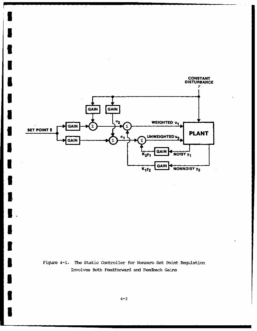
In particular, the principal motivation for OiUS is the problem of vibration

suppression in large lightweight flexible space structures characterized byI high-dimensional, highly uncertain models. In addition, stringent performance

specifications in the face of high disturbance levels place severe demands on

existing control-design techniques. Specifically, performance tradeoffs

involving sensors, processors, actuators, and identification accuracy must be

cut as tightly as possible to minimize hardware and testing costs. For

feasibility and cost effectiveness, system design must also be performed3 efficiently with respect to human and coaputer resources.

The goal of this project has been to develop a mathematically rigorousncontrol-design methodology which directly addresses these technology issues.

In particular, optimal projection theory addresses the need for low-order,I high-performance controllers which can be implemented on-board for real-time

operation. Low-order controllers are necessitated by cost, weight, and

I reliability constraints associated with space-qualified processors.

Furthermore, OPUS incorporates a fundamental theory of robust controller

synthesis to account for unavoidable modeling uncertainties arising for reasons

such as material and manufacturing variations, thermal and aging effects, as

well as limits to identification accuracy. The principal contribution of OPUS

is thus a unified theory which simultaneously accounts for both real-time

processor constraints and modeling uncertainty. A high level overview of OPUS

is given in [88] (Appendix A).

3 During the course of this project OPUS has, in addition, been extended to

a large class of problems in systems and control theory. The current scope of

i the theory includes (see Figure 1-1):

1 1-1

I i-i

ROPETRIC MULTIRATEPONROER CONTROLLER

I IHILERAIL SINGULAR NOISE REDUCED-ORDER SAMPLED-DATA3

CONTOLLE MODLINGCONTOLLE

* ROBU TROLULERROUS STABTY OTRLE

* ROBUSTPERFORMACE * ROBSTIPRMATNCCOTLEIIDSTRNOICUE OTIUU-IM PIA

OEN N UTPROCATINEUAIN STRCTUROEDACINSTSTEAL NOISEOD STNAIT RAISE POINTROL OLE

ENERGY AALYSIS'

FIX

Fiur . Scope of OPUSRO

j II

I 1. A unified treatment of reduced-order modeling, estimation, andcontrol (Appendix B);

£ 2. Robust estimation and control via quadratic Lyapunov functionsincluding robust performance (Appendices G,H,I);

3 3. A unified approach to 2 and H. control including parametricrobustness (Appendix J);

4. Decentralized, nonstrictly proper, and sampled-data control(Appendices D,E,L).

Of particular interest is the recent extension to H, control. As shown in

(117] (Appendix J), we have developed a method for directly imbedding H, design

constraints within OPUS theory and thus, in particular, within LQG. These

results are given by a system of modified Riccati equations which directly

generalize IQG theory and which have the potential for significant

i computational savings compared to existing H synthesis methods.

3 The underlying philosophy of OPJS is to capture as many design

constraints as possible within a single system of design equations. This is

I demonstrated in (117] by the unification of time- and frequency-domain

criteria addressed by the L2/1-6 design equations. An additional example isI provided by the results obtained in (119,94] (Appendices H and I) for robust

stability and performance via fixed-order compensation in the presence of real-

valued structured parameter uncertainty. In these algebraic design equations

I the projection matrix automatically enforces a constraint on controller order,

while additional terms guarantee both robust stability and performance. Note

I that for full-order controllers in the absence of uncertainty, these four

coupled equations reduce to the standard pair of separated Riccati equations of

i LQG theory. Versions of these equations have been developed for each of the

problems shown in Figure 1-1. These results are discussed in more technical

detail in the following sections.

The justification for this line of research is based upon several

i considerations. First, and most obvious, is the fact that our results show

that numerous design constraints can be captured simultaneously within a

constructive theory which directly generalizes LQG theory. Such an approach

provides the capability for simultaneously performing multiple design tradeoffs

* 1-3

I

for multivariable systems with respect to competing constraints such as sensor

noise, control authority, controller order, robustness, disturbance

attenuation, mean-square error, sample rate, degree of decentralization, etc.

Next we stress that rathe- than being ad hoc constructions, these design

equations follow directly from the optimality of well-defined performance Iobjectives. Thus, these results are useful in assessing the suboptimality of

alternative methods. For example, as shown in [20] several suboptimal 3approaches to reduced-order control design can be viewed as approximations to

the optimal projection equations. 31.2 Status of Computational Results

Overall, OPUS can be viewed as a theory for characterizing solutions to

constrained control-design problems. Transforming OPUS into a practical design 3methodology requires the development of effective computational algorithms.

Such development has been carried out in related work by S. Richter at Harris

Corporation. Using homotopic continuation methods, Richter has developed

efficient algorithms which fully account for the structure of these modified

Riccati equations and their coupling terms. Homotopy algorithms, as reviewed

inI

S. Richter and R. DeCarlo, "Continuation Methods: Theory andApplications," IEEE Trans. Autom. Contr., Vol. 28, pp. 660-665,1983.

offer several advantages over both gradient-based and Newton-type methods. UFor example, homotopy methods have a strong theoretical foundation based upon

differential topology, in particular, topological degree theory, while in

practice these methods effectively address the key issues of startup,

convergence, and global optimality. Homotopy algorithms have also reached a 3high degree of maturity and availability with the advent of HOMPACK described

in,

1-4 1I

i L. T. Watson, S. C. Billups, and A. P. Morgan, "A Suite of Codesfor Glcally Convergent Hcmotopy Algorithms," AC4 Trans. Math.3 Software, Vol. 13, pp. 281-310, 1987.

The continuation algorithm developed for the optimal projection equations

essentially follows a smooth path connecting an easily solvable version of theequations with the final, desired form. The algorithm utilizes the tensor3 derivatives of the terms in the optimal projection equations to integrate along

the solution paths. To demonstrate the algorithm, an 8th-order, nonminimum

i phase example originally due to

R. H. Cannon, Jr., and D. E. Rosenthal, "Experiments in Controlof Flexible Structures with Noncolocated Sensors and Actuators,"AIAA J. Guid. Contr. Dyn., Vol. 7, pp. 546-553, 1984.

I was considered. This problem was used in

I iY. Liu and B. D. 0. Anderson, "Controller Reduction Via StableFactorization and Balancing," Int. J. Contr., Vol. 44, pp. 507-£ 531, 1986.

to compare several reduced-order control-design methods. The comparisons

performed by Liu and Anderson highlight the suboptimal nature of these

methods. Specifically, several methods failed to yield stabilizing3 controllers for 10% of the cases while others failed for as many as 60%. In

contrast, as reported in (68,102], the optimal projection approach yielded

i stabilizing controllers for all cases considered. While the methods compared

by Liu and Anderson were most prone to failure at high authority levels, the

optimal projection results were within 20% of the LQG performance at 102-103

higher authority levels. In addition, using topological degree theory, anupper bound has been obtained on the number of solutions of the design

equations. Letting n = plant dimension, nu = dimension of the unstable plant

subspace, nc = compensator order, .9 = number of measurements, and m = number of

I controls, the number of solutions for the case n>. nu is not greater than

* 1-5

I

,n c :s min (n, m,.z),

1 , otherwise. n

Hence, for the case in which the controller order is greater than the number of

inputs or outputs (so that the controller is not ill-conditioned), the 3equations possess at most one solution corresponding to the global minimum.

Furthermore, since in many practical cases of interest this bound is small, it 3suffices to compute each such solution to determine the global optimum. These

results along with suitable extensions to related problems have been used 3widely throughout this project. For example, recent results on fixed-order

control of distributed parameter systems described in Section 2.3 were obtained

using the homotopy algorithm.

1.3 LonQ-RanQe Goals of the Project 3The long-range (5-10 year) goal of this project is the development of a 3

truly effective computer-aided design methodology for multivariable control

design. Numerical solution of the design equations would form the basis for 5such a design tool. This methodology would be appropriate in an engineering

environment since the user need not be familiar with the mathematics of the

design equations being solved. We envision a methodology similar to finite Ielement modeling used routinely by structural analysts. An OPUS design package

would go far beyond currently available packages whose multivariable design 3capabilities are based largely upon LQG theory.

1.4 Plan of This Report n

Since this is the final report for this project our goal is to accomplish Ithe following objectives:

1) Review the evolution and maturation of the research plan throughoutthe project; 3

2) Highlight the principal research accomplishments; and

1-6 1I

II

3) Sumiarize open problems and point out future research directions.

Detailed technical discussion of results obtained will not appear in the main

I body of the report. Rather, the appendices contain a fairly complete (and

lengthy) collection of the principal research results. We note that therordering of the appendices is not chronological but instead reflects the most

logical order according to subject matter.

I1I'I

IIIIIIiII

Ii 1-'7

I

III3IIIII3 SECflON 2.0

FIXED-ST~JCIURE DFSI~

IIIIIIIII

I

2.0 FIXED-STRUCIURE DESIGN

1 2.1 Motivation

3 While achieving the system design specifications (stability, performance,

etc.) the control-design process must not lose sight of restrictions which

m arise in controller implementation. Indeed, control-design methods which

focus primarily on performance specifications often pay a serious price byI producing controllers which are difficult, if not impossible, to implement in

practice. Hence our approach rests upon the notion of fixed-structure design.i That is, we seek to meet design specifications within a framework which

constrains the class of implementable designs. In this way the burden of

hardware implementation (sensors, processors, and actuators) can be minimizedI to the greatest possible extent.

3 2.2 The Three Basic Problems

The most fundamental restriction arising in fixed-structure design is

that of the order, or dimension, of the controller. In addressing this

problem we have developed a unified treatment of three basic problems in

reduced-ordersign, namely, modeling, estimation, and control. These three

problems form a fundamental hierarchy of design problems in system theory,U namely, to determine a system of fixed degree which, for a given system,

approximates, estimates, or controls selected plant states. The solutions toI these problems, given in (32,29,24] (Appendix B), reveal a surprising degree of

common structure. Specifically, the solutions involve systems of 2, 3, and 4I modified algebraic Riccati and Lyapunov equations coupled by a projection

matrix (the "optimal projection"). In addition, the estimation and control

results provide transparent generalizations of steady-state Kalman filter andI tQ theory.

I Although the structure of these equations is aesthetically appealing by

itself, the principal benefit for practical purposes is computational. ThatI is, by exploiting the structure of these equations it is possible to

significantly reduce the computational burden inherent in commonly used

I 2-1

Im . .. , , | i

I

gradient search techniques. This point has been amply demonstra-CA in (63,68] l

as discussed in Section 1.

2.3 Finite-Dimensional Control of Distributed Parameter Svstems

The problem of controller order becomes exacerbated when the plant isinfinite dimensional since infinite-dimensional controllers cannot beimplemented precisely, while finite-dimensional plant approximations may be ofarbitrarily high order. To address this problem the fixed-structure control- 3design results of [24] were generalized in [37] (Appendix C) to the case inwhich the plant is infinite dimensional. The resulting design equations now

comprise a system of four operator equations coupled by a finite-ranknonselfadjoint projection operator. In spite of the infinite dimensionality ofthe plant, the design equations directly characterize fixed-order, finite- 3dimensional dynamic compensator gains (Figure 2-1). Corresponding results forfixed-order finite-dimensional modeling and fixed-order finite-dimensional 1state estimation can also be obtained in an analogous manner.

Application of the operator-theoretic results of [37], however, requiresfinite-dimensional approximation of the design equations. In practice one

could solve the design equations for a sequence of plant approximations of Iincreasingly high order while keeping the controller order fixed. The limitingcontroller would then serve as a nearly optimal fixed-order finite-dimensional 3controller for the original distributed parameter system (Figure 2-2). Thiswas investigated numerically in [122] in a collaborative project with Professor 3I. G. Rosen. In [122] two alternative approaches were considered for obtainingfinite-dimensional controllers for infinite-dimensional systems. The firstapproach, which has been widely studied, involves computing a sequence of full-order iQG controllers for a sequence of high-order plant approximations, while

the second approach assumes a fixed order for the dynamic controller. To Idemonstrate these methods, two examples were considered, namely, a one-dimensional parabolic (heat/diffusion) system and a hereditary (delay) system.For each example a sequence of spline-based, Ritz-Galerkin finite elementapproximations was derived for use in the control-design procedure. LG theory

and the optimal projection approach were then used to obtain full- and first-

2-2 1I

IIIUI i

I

IIII

Figure 2-1. The Optimnal Projection Equations For Finite-Dimensionall Fixed-Order Dynamic Compensation of Infinite-Dimensional Systems

Provide a Direct Path to Optimal Physically Realizable Controllers forDistributed Parameter Systm

I 2-3

I

. . .. . . , l l l l l l I I I I

IIII

CONVERGENCE OF SUBOPTIMAL REDUCED-ORDER COMPENSATORS

IDEA: DESIGN A SEQUENCE OF REDUCED-ORDER COMPENSATORS IWHILE INCREASING THE ORDER OF THE APPROXIMATE MODELAND KEEPING THE ORDER OF THE COMPENSATOR FIXED

n"' ORDER DISTRIBUTEDAPPROXIMATE MODEL PARAMETER SYSTEM

DISCRETIZATION3FAw", B (n), C(n) n-A B, C

(Matrix Form) ",,(Operator Form) .,.,,

NUMERICAL AGRTM

Fn--oo -i a Me.Bev c i

Cnh ORDER COMPENSATOR: (n Fxe) ORDER COMPENSATOR:I

OPTIMAL FOR nth ORDER OPTIMAL FOR DISTRIBUTEDAPPROXIMATE MODEL PARAMETER SYSTEM

III

Figure 2-2. Numerical Solution of the Optimal Projection Equations for

Fixed-order Dynamic Copestion Provides a Path to the

Optimal Fixed-Order Controller for an Infinite-Dimensional system

2-4I

I, , , ORE COPNSTR I I RERCMPNATR

I order controllers for each example with plant approximations up to 32nd order.

i For the parabolic system the performance degradation of the first-order

controllers was only 2% compared to the full-order controllers (Figure 2-3),

while for the hereditary system the degradation was less than 10%. The

difference in implementation requirements for a first-order versus a 32nd-order

controller is, of course, considerable.

2.4 Decentralized Control

I In addition to incorporating constraints on the order of the feedback

compensator, the fixed-structure approach allows additional constraints on the

conplexity of the feedback law. In particular, the results of [24] assumed a

centralized structure for the dynamic compensator. In many applications,

however, a decentralized controller architecture permits a simplified feedback

communication structure and allows increased parallelism in the control law

S execution.

The fixed-structure approach is ideally suited to the decentralizeddesign problem. For each fixed decentralized architecture, the design

I procedure can be performed to assess the ability to meet specifications for the

given configuration. If specifications cannot be met, then the feedback

architecture can be modified to improve performance, robustness, etc.IiFor the case of dynamic compensation, it was shown in [76] that the

I optimal projection technique provides a direct means for characterizing

decentralized controllers. The key step is the realization that each

I subcontroller in the decentralized configuration must be an optimal

centralized controller when viewed as a controller for the plant and remainingsubcontrollers. This observation imediately suggests a sequential design

algorithm in which individual subcontrollers are alternately refined until

convergence is achieved. Because the method is based upon optimization

I principles, performance improvement is guaranteed at each step. This technique

was demonstrated numerically in [76] (Appendix D) where a two-channel

I decentralized controller, fourth-order in each channel, was designed for a pair

of interconnected simply supported beans. The algorithm demonstrated

I 2-5

I

Exect Cpen Leon Cost3

75.01

70.0-

B5.0

w0.0I

tO I 2025 101

PLANT APPROXIMATION ORDER

Figure 2-3. The LQG Closed-Loo0p Cost via Full-Order Controllersis Compared to First-order optimal Projection Designs

for a Parabolic system

2-61

II

convergence to a decentralized controller whose performance was within 10% of

I the fully centralized controller.

For the case in which each subcontroller is a static (proportional)

I feedback law, it is possible to simultaneously characterize the optimal gains

in each control channel without requiring a sequential approach. A thorough

I treatment of this case, including robust stability and performance, is given in

[121] (Appendix D).

I i 2.5 Singular Control

An important generalization of the results of (24] involves the case in

which the controller includes a static feedthrough component. One technical

i issue which arises in the problem formulation is that the L2 norm of a control

signal corrupted by white noise (as a result of measurement feedthrough) is

infinite. Hence the measurement feedthrough problem is only well-posed when

either the measurement noise intensity or the control weighting matrix issingular. As is well known from the singular control literature, however,

singular problem data often lead to complex behavior including impulsive

controls and singular arcs. The imposition of a smooth controller structure

I via the fixed-structure approach thus precludes such complex behavior.

The fixed-order state estimation and dynamic compensation results of[29,24] were partially extended to the singular case in [78,79]. Even in theU full-order case the singular control results are novel since standard LQG

theory yields only strictly proper controllers. The results of [78,79] were

incomplete, however, since the gains associated with certain estimation and3 feedback paths were not given explicitly. For the singular estimation problem

this defect was remedied inIY. Halevi, "The Optimal Reduced-Order Estimator for Systems withSingular Measurement Noise," IEEE Trans. Autom. Contr., Vol. 34,3 1989.

I where all feedback gains were explicitly characterized. In addition, this

i 2-7

i

I

solution was shown to agree c letely with results obtained using standard

limiting methods. For the corresponding dynamic-compensation problem the

ocuplete singular solution has been derived in joint research with Professor Y.

Halevi and will be reported in [130,138,139] (Appendix E).

IIIIIIIIIIIII

2-8 I

U

UIIIIIIII

SECITON 3.0

i~aisr ANWLSIS AND D~SIG~I

IIIIIIIII

13.0 ROBUST ANALYSIS AND DESIGN

1 3.1 Motivation

The purpose of feedback control is to achieve desirable performance in theface of uncertainty. Although identification can reduce uncertainty to some

i extent, it is often impractical and residual modeling discrepancies always

remain. For example, modeling uncertainty in flexible structures may arise in

the mass, dampin, and stiffness operators. Controllers must therefore be

robust to achieve desired disturbance rejection in the presence of suchS modeling uncertainty.

3.2 Stochastic Modeling

Our approach to robust control was originally inspired by stochastic

I parameter modeling within a linear-quadratic optimization framework. In a

series of early papers [1-16], D. C. Hyland explored the ramifications of aI multiplicative white noise model as a consequence of the minimum information

modeling technique based upon the Maximum Entropy Principle of Jaynes. Theintent was not to view the white noise process as a literal model of parameter

uncertainty, however, but rather to construct a tractable design model which

captures the effects of parameter uncertainty upon system performance.IIAn interesting feature of the Maximum Entropy modeling approach was that

I the multiplicative white noise model was not to be rigorously interpreted as an

Ito differential model, but rather in terms of the Stratonovich formulation.

Recasting the Stratonovich model in terms of Ito differentials then led to

additional "correction" terms. It is precisely these terms which were shown toplay a crucial role in capturing the effects of parameter uncertainty. Such

effects include decorrelation, i.e., the decrease in cross-correlation ofsystem states due to parameter uncertainty, as well as equilibration, i.e., theI tendency of state variances to equalize in the presence of high levels of

uncertainty thus rendering different states indistinguishable. 2hese effectsI of parameter uncertainty are fundamental features of high-order, lightly damped

modal systems. An interesting treatment of these ideas for structural and

* 3-1

I

acoustic analysis can be found in I

R. H. Lyon, Statistical Energy Analysis of Dynamical Systems: iTheory and Aplication, MIT Press, Cambridge, MA, 1975.

For feedback design within fixed-structure design theory, the

Stratonovich model produces controllers possessing intuitively appealing

features. Specifically, such control laws exhibit high-authority control in

the low-frequency, well-modeled portion of the structure along with low-

authority, rate dissipative action in the high-frequency region [35] (Appendix

F). The ability to merge and unify these control regimes is a unique and

significant contribution of the Maximum Entropy approach. 3As a control-design methodology, however, it remained to validate the

approach as a rigorous robust design technique. Optimal controllers designed

in the presence of white noise disturbances, it was reasoned, are

automatically desensitized to actual deterministic plant parameter variations.

This idea was confirmed empirically by numerical studies in [36,39] which

showed an efficient design tradeoff between performance and robustness in the

presence of structured real-valued parameter variations. Further robustness

studies confirming these results were carried out in

A. Gruzen, "Robust Reduced Order Control of FlexibleStructures," C. S. Draper Laboratory Report #CSDIT9 00, April1986.

A. Gruzen and W. E. Vander Velde, "Robust Reduced-Order Controlof Flexible Structures Using the Optimal Projection/MaximumEntropy Design Methodology," AIAA Guid. Nay. Contr. Conf.,Williamsburg, VA, August 1986.

M. Cheung and S. Yurkovich, "On the Robustness of MEOP Designversus Asymptotic LQG Synthesis," IEEE Trans. Autom. Contr., Vol.33, 1988.

In spite of these results, it was clear that issues concerning stochastic 3modeling, such as stochastic stability and the physical interpretation of the

model, tended to obscure the effectiveness of the technique for robust

control. Thus a crucial step in the evolution of our approach was the ability

3-2 i3

Ito show in (771 (Appendix F) that such controllers are guaranteed to be robustI for all cases in which the design equations are solvable. In particular, it

was shown that a second-mament stochastic stability condition in the presenceI i of a time-exponential cost weighting induces a Lyapunov function which

guarantees deterministic robust stability over a prescribed range of parameter

variations. This result thus provided the bridge to cross over from the worldI of stochastic modeling (a statistical theory) to deterministic robustness

theory (a theory of worst-case bounds).

3.3 Robust Analysis

I For a given controller, it is often necessary to assess the stability andI worst-case performance of the closed-loop system as parameters vary within aspecified range of uncertainty. This is a problem of robust analysis, whose

consideration precedes the more complex problem of robust controller synthesis.

our principal mathematical technique in robustness analysis is Lyapunov

I stability theory. Here the idea is to determine a Lyapunov function which

guarantees robust stability over a range of uncertain parameters. For linearI systems we enploy the quadratic Lyapunov function

V(x) = xTpx (1)

or, equivalently, the Lyapunov equation

S0 = ATP + PA + R (2)

I for the linear system

I = Ax + w. (3)

I The dual equation

0 = AQ + QAT + V (4)

I 3-3

I

is also useful for robust performance analysis since V can be interpreted as

the intensity of the additive white noise signal w. In robust analysis one

typically replaces (4) by

I0 = AQ + QAT + n + V, (5)

where n is an additional nonnegative-definite matrix. Now robust stability of

the perturbed system

= (A+&iA)x + w (6) l

is assured so long as liAAQ + QA T < n. (7) I

This can be seen by rewriting (5) as

0 = (A+4A)Q + Q(A+stA) T + [n- &A T) ] + V. (8)

Furthermore, it is also possible to guarantee robust performance since the

solution O&A of I0 = (A4&A) QA + Q&A(A+t&A)T + V (9)

satisfies

_<Q . (10) IThe above technique, developed in [115] (Appendix G), provides a simple

3-4 1I

I

i approach to robust stability and performance.

m To develop a more sophisticated approach one can replace (5) by

m O=AQ+QAT+f(Q) +V (11)

I where fl(.) is now a bounding operator which satisfies

3 AAQ + OiAT < n (Q) (12)

for all variations &A in a specified uncertainty set and for all nonnegative-

definite matrices Q. This approach now guarantees the bounding a priori via

(12) and the problem is to determine whether or not there exists a solution to

The a priori bounding technique shown in (11), (12) has been given a

fairly complete treatment in [123] (Appendix G). The goal in [123] was to

I systematically investigate candidate choices for the function n(.). This

investigation also provides a unified setting for particular bounds which have

I been used in various control-design contexts. For example, for A= al, jaI 1 ,

the absolute value bound

I n(Q) = IAQ + QAlT, (13)

i where 1" replaces each eigenvalue by its absolute value, was proposed in

i S. S. L. Chang and T. K. C. Peng, "Adaptive Guaranteed CostControl of Systems with Uncertain Parameters", IEEE Trans.Autom. Contr., Vol. AC-17, pp. 474-483, 1972.

5 On the other hand, writing A1 = DIE1 , the bound

3 n(Q) = D + QEQ, (14)

* 3-5

I

where D = DIDIT and E = E TEj1 , was studied in

I. R. Petersen and C. V. Hollot, "A Riccati Equation Approach tothe Stabilization of Uncertain System", Automatica, Vol. 22, Ipp. 433-448, 1986.

D. Hinrichsen and A. J. Pritchard, "Stability Radius for UStructured Perturbations and the Algebraic Riccati Equation",Sys. Contr. Lett., Vol. 8, pp. 105-113, 1986.

Finally, the choice

n(Q) = aQ + a-lAIQAIT (15) Icorresponds to the bound arising from a multiplicative white noise model as

discussed in (77] and Section 3.2. We call (14) the quadratic bound (since it

is quadratic in Q) and (15) the linear bound (since it is linear in Q).

3.4 Robust Synthesis i

The principal payoff of our robust stability and performance technique is ithe ability to incorporate these bounds directly within the fixed structure

design methodology. This can be done by bounding the cost over the class of 3parameter uncertainties prior to determining the feedback gains. The resulting

bound is then treated as an auxiliary cost which can then be minimized by

suitable feedback gains. The solution to this optimization problem is thus

guaranteed to yield robust stability and performance.

To carry out this procedure it is essential that the bound n(. ) be Idifferentiable with respect to Q. Furthermore, D(.) will be differentiablewith respect to the feedback gains if it is differentiable with respect to A1

(which involves gains in the control-design setting). These requirements thus

suggest the linear bound (15) and the quadratic bound (14) as the prime

candidates for robust synthesis.

3-6 i

I

i As discussed previously, the linear bound (15) was originally suggested byi a multiplicative white noise model. By incorporating this bound within the

design procedure, sufficient conditions for robust estimation and robust

control were developed in [95,119] (Appendix H). In addition, a unified

treatment of robust, reduced-order modeling, estimation, and control was given

in [ 89 ] (Appendix H).-

The quadratic bound (14) has also been developed extensively within a

i design context. In [101,83,94] (Appendix I) the problems of reduced-order

modeling, estimation, and control were considered via this bound. Finally,

both the linear and quadratic bounds were considered simultaneously in [113]

(Appendix I).

3.5 H Theory

The robustness theory discussed in the previous subsections addresses the

problem of real-valued structured parameter uncertainty. In many

applications, however, uncertainty is present in the form of unstructured

perturbations to the plant transfer function. A typical case is the presence

i of high-frequency, unmodeled dynamics.

A mathematically rigorous approach to this problem involves defining a

I suitable norm on the space of plant transfer functions to characterize

uncertainty in terms of neighborhoods of the nominal plant. The resulting HO

I theory was pioneered by Zames in

G. Zames, "Feedback and Optimal Sensitivity: Model ReferenceTransformations, Multiplicative Seminorms, and ApproximateInverses," IEEE Trans. Autom. Contr., Vol. AC-26, pp. 301-320,1981.

while recent overviews were given in

B. A. Francis and J. C. Doyle, "Linear Control Theory with an H.Optimality Criterion," SIAM J. Contr. Optim., Vol. 25, pp. 815-844, 1987.

* 3-7

I

I

B. A. Francis, A Course in & Control Theory, Springer-Verlag, nNew York, 1987. 1

The most fundamental problem of Ho control design is the so-called

Standard Problem considered by Francis: determine a feedback compensator

which minimizes the peak (worst-case) disturbance attenuation of the closed-

loop system. By introducing suitable weighting matrices and problem

transformations, solutions to the Standard Problem can be used to yield robust

controllers for unstructured plant uncertainty.

Current F. synthesis methods, however, possess two principal drawbacks:

they are computationally intensive and they often yield excessively high-order

controllers. These difficulties have been removed with the advent of new state

space solutions to the Standard Problem given in [117] (Appendix J) and

I. R. Petersen, "Disturbance Attenuation and IH Optimization: ADesign Method Based on the Algebraic Riccati equation," IEEETrans. Autom. Contr., Vol. AC-32, pp. 427-429, 1987.

P. P. Khargonekar, I. R. Petersen, and M. A. Rotea, "Il OptimalControl with State Feedback," IEEE Trans. Autom. Contr., Vol. 33,pp. 786-788, 1988.

J. C. Doyle, K. Glover, P. P. Khargonekar, and B. A. Francis, I"State-Space Solutions to Standard H2 and H. Control Problems,"Proc. Amer. Contr. Conf., pp. 1691-1696, Atlanta, GA, June 1988.

These papers characterize solutions to the Standard Problem in terms of

modified Riccati equations. The computational savings of this approach over

earlier methods is considerable, possibly two orders of magnitude. In

addition, the dynamic compensators obtained from these Riccati equatioys are of

the same order as the plant model. This approach thus removes the principal

drawbacks of earlier 16 synthesis methods. UBy incorporating the fixed-structure approach we have, in addition,

obtained the most general solution thus far available for the Standard

Problem. Specifically, in [117] (Appendix J) we consiCd2r the minimization of

an L performance criterion subject to a constraint on the HF closed-loop

performance. This multi-norm problem formulation thus allows the designer to

3-8 1I

perform tradeoffs between these caripetinq performance measures. In addition wei impose a constraint on the order of the dynamic compensator to obtain optimal

low-order feedback controllers which satisfy the H. performance constraint.U Utilizing an eighth-order nonminimum phase example given in

R. H. Cannon, Jr., and D. E. Rosenthal, "Experiments in Controlof Flexible Structures with Noncolocated Sensors and Actuators,"AIAA J. Guid. Contr. Dyn., Vol. 7, pp. 546-553, 1984.

E we used these results to obtain 9 dB improvement over the corresponding LQGdesign (Figure 3-1).

Immediate spinoffs of these results include the problems of model

i reduction and state estimation. The H. model reduction problem [114]

(Appendix J) addresses one of the most fundamental problems of linear systemtheory, namely, given a linear time-invariant system of degree n, find a linear

time-invariant transfer function of degree nm<n which minimizes the H. distancebetween the full- and reduced-order systems. Although the Hankel norm model-

I reduction problem has been widely studied as in

K. Glover, "All Optimal Hankel-Norm Approximations of LinearMultivariable Systems and Their L'?-Error Bounds," Int. J.Contr., Vol. 39, pp. 1115-1193, 1984.

I the solution to the Hw problem had not been given previousl ,.

I For state estimation the Kalman filter provides the least squares (12)optimal solution. In certain applications, however, it may be desirable to

minimize the worst-case frequency content of the error signal. This problem isaddressed in [116) (Appendix J) where the standard steady-state Kalman filter

I is generalized to include a bound on the F6 norm of the error signal.

Finally, it is reasonable to expect that in practice both structured andunstructured plant uncertainty will be present. This leads to consideration of

i the Standard Problem in the presence of parametric uncertainty. Thus it is ofinterest to design feedback controllers which are guaranteed to satisfy a

* 3-9

I

I

II

FREG (HZ] Ito, 3 LQG 10'-2 1o0'-1 1 10

0.0

-10.0 1cc -20.0

cc -3G.0 3z -40 .0 3

-50.03

-6O.O -!

II

Figure 3-1. The LQG/Hw Design Equations Yield 9 dB Improvenent Over TheCorresponding LQG Design for an 8th-Order Nonminimum Phase Plant

3-10 1

I

I specified H disturbance attenuation constraint over a range of parametric

i uncertainty. This problem has been addressed in (105] (Appendix J) where the

results of [117] on H. design have been merged with these of [94,1191 on

parametrically robust design. Again the development has been carried out in

the context of fixed-order dynamic conpensation for maximal design flexibility.

II

I,II!,I

I"III

I 3-1i

I

IIIIIIIII3 SECTION 4.0

FtJR~ER EXrENSIONS

I3IIIIIII

I

4.0 FURTHER EXTENSIONS

1 4.1 Motivation

I The previous sections have addressed two principal problems in control

design, namely, fixed-structure design and robustness. Both of these problems

concern fundamental issues in the practical implementation of feedback

controllers. In this section we extend these results in two directions in

I norder to address largex classes of design problems.

D 4.2 T

All of the feedback control theory discussed in Sections 2 and 3

addresses the problem of feedback control for regulation in the presence of

external disturbances. Many control problems, however, are of a tracking or

I servomechanism nature. While a limited class of such problems can be recast

without loss of generality as regulation problems, many important ones cannot.3 For example, the standard transformations given in

H. Kwakernaak and R. Sivan, Linear Optimal Control Systems,Wiley, New York, 1972.

B. A. Francis, A Course in H Control Theory, Springer-Verlag, New3 York, 1987.

I assume that the comand signals can be represented as an augmentation of the

plant dynamics. There are many important cases, such as the tracking of steps

and raqps, which must be represented by uncontrollable, unstable dynamics,

where this transformation cannot be applied. Furthermore, such

transformations often ignore controller effort. To fill this gap we have

undertaken a systematic program for developing a tracking control theory

consistent with earlier developments. As a first step we have considered the

I problem of regulation about a prescribed nonzero set point, which corresponds

to the step command tracking problem. Our work in this area was originally

S motivated by results obtained in

3 4-1

I

I

Z. Artstein and A. teizarowitz, "Tracking Periodic Signals withthe Overtaking Criterion," IEEE Trans. Autan. Contr., Vol. AC-30,pp. 1123-1126, 1985. 3A. Teizarowitz, "Tracking Nonperiodic Trajectories with theOvertaking Criterion," Appl. Math. Optim., Vol. 14, pp. 155-171, 1986. UA. leizarowitz, "Infinite Horizon Stochastic Regulation andTracking With the Overtaking Criterion," Stochastics, 1987.

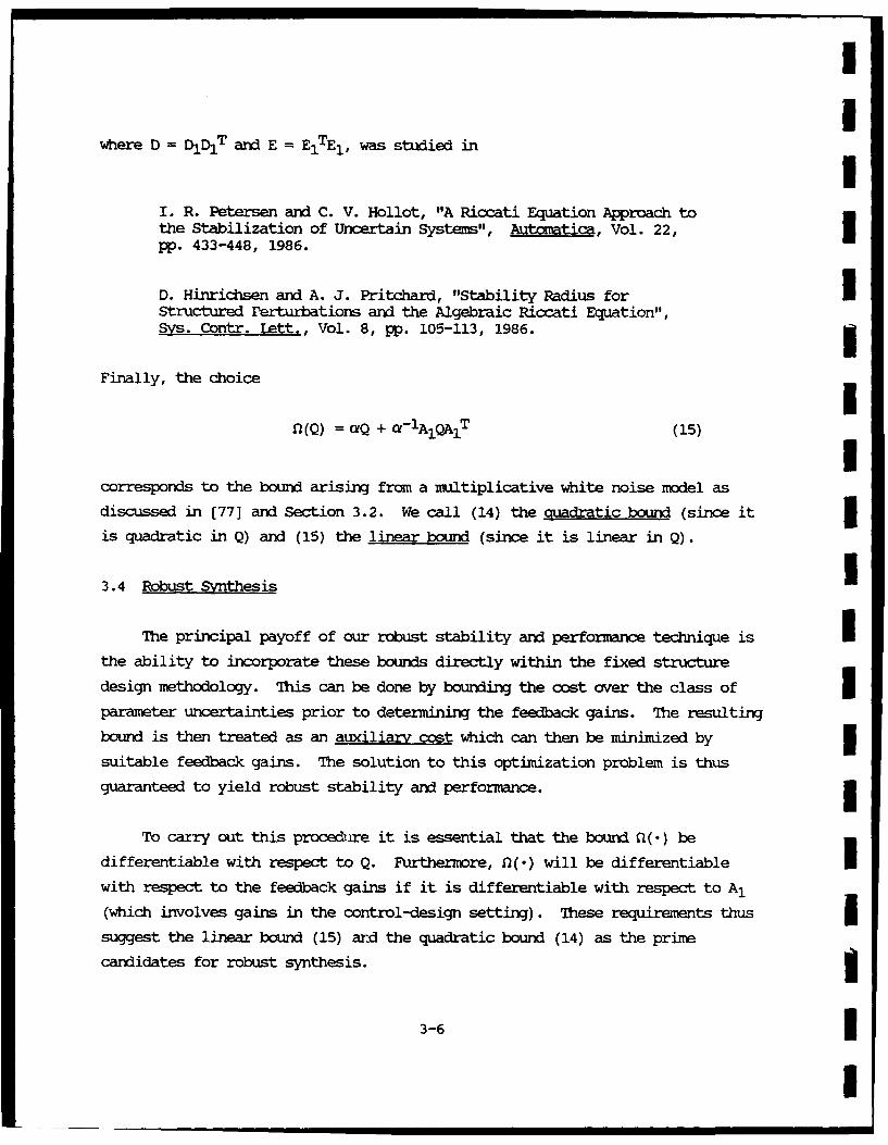
References (67,103] (Appendix K) present general solutions to the nonzero set 5point problem for both static and dynamic controllers. The overall controller

configurations for these problems are shown in Figures 4-1 and 4-2. Note that

these controllers involve two components, namely, a closed-loop feedback icomponent similar to a regulator and an open-loop feedforward component which

has no counterpart in the standard theory and which cannot be obtained from 3standard transformations.

Recent activities have focused on extending the nonzero set point results

to broader classes of command and disturbance signals. It turns out that the

challenging case (as with steps and ramps) involves signals generated by

unstable command or reference dynamics. As a critical first step in addressing

this problem we have considered the problem of reduced-order steady-state Iobserver design for unstable plants. These results appear in (125] (Appendix

K). This optimal subspace observer problem gives rise to yet another

projection which we denote by g. The most general estimation problem involving

all three projections r, v, and / has also been solved and will be reported in

[134,139].

4.3 Samled-Data Control iThe discussion in the previous sections has focused on continuous-time 3

systems subject to continuous-time (analog) controllers. In practice, however,

controller implementation will almost invariably utilize digital controllers

within the context of sampled-data control systems. Rigorous consideration of

such systems is critical, particularly for distributed parameter systems which

possess modal frequencies beyond the Nyquist rate of any digital ontroller.

4-2 1I

CONSTANTI DISTURBANCE

GAIN GAI

KIY2 -FAN NONNOISY Y2

ft Figure 4-1. The static Controller for Nonzero Set Point RegulationInvolves Both Feedforward and Feedback Gains

1 4-3

IIII

_ DISTURBANCEI

OFFSET Y

r [ N'D , TUISTURBANCE

I

I

COMPENSATOR c GAIN

GAIN

• I I

III

Figure 4-2. The Dynamic Controller for Nonzero Set Point Regulation

Involves Both an Open-Loop Gain and a Closed-Loop Dynamic Compensator

4-4 I

I

Hence, a rigorous theory of sampled-data control design must be developed which

I accounts precisely for all effects arising frcm analog-to-digital and digital-

to-analog operations.

U Optimal projection theory for discrete-time system was developed in [41]

and applied to sampled-data systems in [44] (Appendix L). As a next step it is

desirable to obtain robust control results. To this end, the optimal

projection equations for reduced-order discrete-time estimation and control in

Ithe presence of multiplicative white noise were obtained in [54,69] (Appendix

L). After these results were obtained, it became clear that a true sampled-

I data robustness theory must account for the exponential matrix structure which

arises from the sampling process. For example, if A+i A denotes the continuous-

time dynamics matrix, where A is the nominal matrix and eA denotes uncertainty,

then the equivalent discrete-time dynamics matrix is given by e(A+&A)h, where h

is the sample interval. Because of the exponential function, however, this

discrete-time dynamics matrix does not have the additive structure considered

in the discrete-tim theory in [54,69]. Moreover, a linear approximation for

the exponential will not be valid in the presence of system time constants near

or above the sample rate.

Although an attempt to bound this discrepancy resulted in new

inequalities in [92] and questions of decomposition in [87] (Appendix L), this

approach appears inadequate. The crucial clue to the most natural approach was

ultimately found in

A. R. Tiedemann and W. L. DeKoning, "The Equivalent Discrete-TimeOptimal Control Problem for Continuous-Time Systems withStochastic Parameters," Int. J. Cont., Vol. 40, pp. 449-466,1984.

I which studied the propagation of multiplicative white noise in the presence of

A/D and D/A interfaces. Motivated by these results, we have obtained results

which extend the robust performance bounds obtained for continuous-time systems

to the sampled-data problem. Specifically, by considering the evolution of the

I linear parameter uncertainty bound over the sample interval, a robust stability

1 4-5

i1

condition was developed in [128] (Appendix L). This result is unique in thatI

it accounts directly for the exponential structure of the parameter 3uncertainty.

III ,i

II

I

iII

I. . .,4-6 i III I

IUIIIIIIS3 SECTION 5.0

OPEN P1~)BLENS AND RYIURE DIRECTIONS

USIIIIIIU

I

5.0 OPEN PROBIEM

1 5.1 Motivation

The value and importance of the results obtained under this project lie

largely in the foundation they provide for future research. The purpose ofI this section is to collect together various questions and problems as a guide

to future endeavors. The order of listing of these questions roughly parallels

I the order of the previous sections.

5.2 Fixed-Structure Design

Since the fixed-structure design approach involves a nonconvex3 optimization problem, there arise several questions concerning the structure of

the space of solutions.

* Do there exist verifiable a priori conditions whichguarantee stabilizability of a given linear time-invariantplant by fixed-order dynamic compensation? As in the full-order case, one would expect such conditions to play afundamental role in determining the existence of solutions tothe design equations. Conversely, when the plant is known tobe stabilizable by a controller of order nc, does theunderlying optimization problem always possess a solution?Will the design equations always yield at least one suchstabilizing controller? How is the ability to findstabilizing controllers affected by the choice of weightingsand noise intensities?

I • Is it possible to design all subcontrollers of adecentralized dynamic compensator simultaneously withoutperforming sequential iterations? If a sequential algorithmis used, then under what conditions is the algorithmguaranteed to find the global minimum?

* How can the fixed-structure approach be extended to addressthe simultaneous stabilization problem, i.e., the problem offinding a single controller which stabilizes several5 different plants simultaneously?

The L2 model reduction theory of [32] (Appendix B) canreadily be extended to the problem of characterizing optimalfinite-dimensional models for infinite-dimensional systemsusing the method of [37] (Appendix C). Can such finite-

1 5-1

I

dimensional models serve as useful lumped approximations to Idistributed parameter systems? Can the L2/H6 model reductiontheory of [114] (Appendix J) be used similarly? 3How can the fixed-structure approach be used to designcontrollers with additional constraints on their internalstructure, such as prespecified pole locations? This Iquestion is the basis for ongoing work in [131].

5.3 Robust Analysis and Design II

There exist a variety of open questions concerning the conservatism and

effectiveness of the parametric robustness bounds and the H0O design equations. 5* For which class of parameter uncertainty structures are the

quadratic Lyapunov bounds nonconservative? How can therobustified design equations be used iteratively to reducedesign conservatism?

The multiplicative noise model was shown in [77] (Appendix F)to guarantee deterministic robustness. However, this result Iinvolved a uniform right shift rather than the variable leftshift arising from the Stratonovich interpretation of themultiplicative noise. Can it be shown rigorously that the IStratonovich model yields robust controllers? Furthermore,can the relationship between Stratonovich design and positivereal controllers for modal systems be made precise?

The basis for the HO design results obtained in [117](Appendix J) is the quadratic bound developed forparametrically robust control in [94] (Appendix I). This Iraises the following question: Does there exist analternative interpretation of the linear bound which can beused to guarantee disturbance attenuation for some specifiedclass of disturbances?

The 16 control design results are virtually identical to theoptimality conditions for the problem of minimizing anexponential-of-quadratic cost criterion as considered in I

P. R. Kumar and J. H. van Schuppen, "On the Optimal Control ofStochastic Systems With an Exponential-of-Integral PerformanceIndex," J. Math. Anal. Apl., Vol. 80, pp. 312-332, 1981.

P. Whittle, "Risk-Sensitive Linear/Quadratic/Gaussian Control,"Adv. A=l. Prob., Vol. 13, pp. 764-777, 1981. 1

5-2 1I

A. Bensoussan and J. H. van Schuppen, "Optimal Control ofPartially Observable Stochastic Systems With an Exponential-of-Integral Performance Index," SIAM J. Contr. Optim., Vol. 23, pp.599-613, 1985.

P. Whittle and J. Rkn, "A Hamiltonian Formulation of Risk-Sensitive Linear/Quadratic/Gaussian Control," Int. J. Contr.Vol. 43, pp. 1-12, 1986.

Is it possible to directly extend these results using thefixed structure approach? Also, can the fixed-structureapproach be used to extend the Maximum Entropy theory of

D. Mustafa and K. Glover, "Controllers Which Satisfy a Closed-Loop H. Norm Bound and Maximize an Entropy Integral," Proc. IEEEConf. Dec. Contr., Austin, TX, December 1988.

The LV/1 model reduction theory given in [114] (Appendix J)minimizes an L2 criterion subject to a constraint on the H,distance between the full- and reduced-order models. Can theL2 criterion be neutralized so as to obtain a "pure" H,result as is done in [117] (Appendix J) for full-ordercontrol design? Can the resulting H, solution be shown toactually characterize the H. optimal reduced-order model bytaking the F. constraint to be sufficiently small? Similarquestions apply to fixed-order control design. For exanple,does there exist a "pure" H. reduced-order control designtheory? Can these results be shown to be necessary as wellas sufficient?

What is the generalization of the H,0 control and estimationresults to the singular problem? To the cross-weighting5 problem?

Is it possible to extend the L2 and L2/11. model reductionresults to allow the reduced-order model to be nonstrictlyproper?

I 5.4 Tracking and Sampled-Data Control

With regard to tracking and sampled-data theory a number of problems

remain to be explored.

51 5-3

I

Is it possible to develop a methodology for designingtracking controllers which applies to a broad range ofsignal models? For example, the command signal may be knownexactly in advance (such as a specified square wave) while,at the other extreme, it may only be known to be an elementof a large class of signals. For example, step comands areknown to be steps but their exact level is not known untilthey actually occur during operation. Other command signalsmay only be known to be outputs of system driven by random Inoise. A classification scheme based upon the degree andtype of priori knowledge of the command signal should lead toa hierarchy of control designs ranging from poorly known towell-known command signals. In addition, it is important to 3distinguish between a priori command signal knowledgeavailable during the design phase and command signalknowledge available during operation. The differencesbetween these cases can be used to account for differingassumptions appearing in the literature. Relevant referencesinclude i

B. D. 0. Anderson and J. B. Moore, Linear Optimal Control,Prentice-Hall, Englewood Cliffs, NJ, 1970. IC. D. Johnson, "Accommodation of External Disturbances in LinearRegulator and Servomechanism Problems," IEEE Trans. Autom.Contr., Vol. AC-16, pp. 635-644, 1971.

E. J. Davison and A. Goldenberg, "Robust Control of a GeneralServcmechanism Problem: The Servo Compensator," Automatica, Vol.11, pp. 461-471, 1975.

E. J. Davison, "The Robust Decentralized Control of a GeneralServomechanism Problem," IEEE Trans. Autom. Contr., Vol. AC-21,pp. 14-24, 1976.

E. J. Davison, "The Robust Control of a Servomechanism Problemfor Linear Time-Invariant Multivariable Systems," IEEE Trans.Autom. Contr., Vol. AC-21, pp. 25-34, 1976. £E. J. Davison, "Multivariable Tuning Regulators: TheFeedforward and Robust Control of a General ServomechanismProblem," IEEE Trans. Autom. Contr., Vol. AC-21, pp. 35-47, 31976.

C. A. Desoer and Y. T. Wang, "Linear Time-Invariant RobustServomechanism Problem: A Self-Contained Exposition," inControl and Dynamic Systems, Vol. 16, C. T. Leondes, Ed., pp. 81-129, Academic Press, New York, 1980. 1

5-4 1I

IE. J. Davison and I. J. Ferguson, "The Design of Controllers forthe Multivariable Robust Servomechanism Problem Using ParameterOptimization Methods," IEEE Trans. Autom. Contr., Vol. AC-26, pp.93-110, 1981.

I J. D. Turner, H. M. Chun and J.-N. Juang, "Closed-Form Solutionsfor a Class of Optimal Quadratic Tracking Problems," J. Optim.ZThy. AUL., Vol. 47, pp. 465-481, 1985.

J.-N. Juang, J. D. Turner and H. M. Chun, "Closed-Form Solutionsfor Feedback Control with Terminal Constraints," AIAA J. Guid.3 Contr. Dyn., Vol. 8, pp. 39-43, 1985.

W. E. Sdmnitendorf and B. R. Barmish, "Robust AsymptoticTracking for Linear Systems with Unknown Parameters,"Autanatica, Vol. 22, pp. 355-360, 1986.

How can the new subspace projection A, which arises in theobserver design problem in [125] (Appendix K), be used todesign servoconpensators? That is, can g be used to designcontrollers which track the output of an unstable conmandmodel?

i Is it possible to develop a theory of robust sampled-datacontroller synthesis which accounts directly for theexponential structure of the equivalent discrete-time model?The results of [128] (Appendix L) provide a starting point inthis regard.

* What is the form of the equations for the Hm-constrained3 discrete-time control-design problem?

II

I

I* 5-5

I

IUIUIIIIII SEC~I0N 6.0

OPR~ENSIVE REFERENCE LIST

I3IIIIUII

I1. D. C. Hyland, IThe Modal Coordinate/Radiative Transfer Formulation of

Structural Dynamics-Implications for Vibration Suppression in LargeSpace Platforms," MIT Lincoln laboratory, TR-27, 14 March 1079.

2. D. C. Hyland, "Optimal Regulation of Structural Systems With Uncertain3 Parameters," MIT Lincoln laboratory, TR-551, 2 February 1981, DDC# ADA-099111/7.

3. D. C. Hyland, "Active Control of Large Flexible Spacecraft: A NewDesign Approach Based on Minimum Information Modelling of ParameterUncertainties," Proc. Tird VPI&SU/AIAA Symposium, pp. 631-646,Blacksburg, VA, June 1981.

4. D. C. Hyland, "Optimal Regulator Design Using Minimum InformationModelling of Parameter Uncertainties: Ramifications of the New DesignApproach," Proc. Third VPI&U/AIAA Smosium, pp. 701-716, Blacksburg,VA, June 1981.

5. D. C. Hyland and A. N. Madiwale, '"Minimum Information Approach toRegulator Design: Numerical Methods and Illustrative Results," Proc.Third VPI&SU/AIAA Syvmosium, pp. 101-118, Blacksburg, VA, June 1981.

6. D. C. Hyland and A. N. Madiwale, "A Stochastic Design Approach for Full-Order Compensation of Structural Systems with Uncertain Parameters,"Proc. AIAA Guid. Contr. Conf., pp. 324-332, Alb, NK, August1981.

7. D. C. Hyland, "Optimality Conditions for Fixed-Order DynamicQumpensation of Flexible Spacecraft with Uncertain Parameters," AIAA20th Aerospace Sciences Meeting, paper 82-0312, Orlando, FL, January1982.

8. D. C. Hyland, "Structural Modeling and Control Design Under IncopleteParameter Information: The Maxium Entropy Approach," AFtSI/NASAWorkshop on Modeling, Analysis and Optimization Issues for Large SpaceStructures, Williamsburg, VA, May 1982.

9. D. C. Hyland, 'Minimum Information Stochastic Modelling of LinearSystems with a Class of Parameter Uncertainties," Proc. Amer. Contr.3 onf., pp. 620-627, Arlington, VA, June 1982.

10. D. C. Hyland, "Maximum Entropy Stochastic Approach to Control Designfor Uncertain Structural Systems," Proc. Amer. Contr. Conf., pp. 680-688,Arlington, VA, June 1982.

11. D. C. Hyland, 'inimum Information Modeling of Structural Systems withUncertain Parameters," Proceedin of the Workshop on Applications ofDistributed System Theory to the Control of Larme Space Strucr,G. Rodriguez, ed., pp. 71-88, JPL, Pasadena, CA, July 1982.

3 12. D. C. Hyland and A. N. Madiwale, "Fixed-Order Dynamic CoensationThrvugh Optimal Projection," Proceedins of the Worksho on Avolicationsof Distributed System Theory to the Control of Large Space Structures,£ G. Rodriguez, ed., pp. 409-427, JPL, Pasadena, CA, July 1982.

1

I

I

I13. D. C. Hlylandc, "Me-n-Squre Optimal Fixed-Ode Cc:penstion-BeyondSp ill over" Suppres ion, " paper 1403, AIA Astr dy namics C onrfe rn c,

San Diego, CA, August 1982.

14. D. C. Hyland, "Robust Spacecraft Control Design in the Presence ofSensor/Actuator Placement Errors;" AIAA Astrodynamics Conference,San Diego, CA, August 1982.

15. D. C. Hyland, "The Optimal Projection Approach to Fixed-OrderCompensation: Numerical Methods and Illustrative Results," AIAA 21st IAerospace Sciences Meeting, paper 83-0303, Reno, NV, January 1983.

16. D. C. Hyland, "Mean-Square Optimal, Full-Order Compensation of StructuralSystems with Uncertain Parameters," MIT Lincoln Laboratory, TR-626, 3

1 ue1983.

17. D. S. Bernstein and D. C. Hyland, "Explicit Optimality Conditions for IFinite-Dimensional Fixed-Order Dynamic Compensation of Infinite-Dimensional Systems," presented at SIAM Fall Meeting, Norfolk, VA,November 1983.

18. D. C. Hyland and D. S. Bernstein, "Explicit Optimality Conditions forFixed-Order Dynamic Compensation," Prcx.. 22nd IEEE Conf. Dec. Contr.,pp. 161-165, San Antonio, TX, December 1983.

19. F. M. Ham, J. W. Shipley and D. C. Hyland, "Design of a Large SpaceStructure Vibration Control Experiment," Proc. 2nd Int. Modal Anal. IConf., pp. 550-558, Orlando, FL, February 1984.

20. D. C. Hyland, "Caparison of various Controller-Reduction Methods:Suboptimal Versus Optimal Projection," Proc. AIAA Dynamics SpecialistsCon., pp. 381-389, Palm Springs, CA, May 1984.

21. D. S. Bernstein and D. C. Hyland, "The Optimal Projection Equations for IFixed-Order Dynamic Ccpensation of Distributed Parameter Systems,"Proc. AIAA Dynamics Specialists Conf., pp. 396-400, Palm Springs, CA,May 1984. 1

22. F. M. Ham and D. C. Hyland, "Vibration Control Experiment Design for the15-M Hoop/Column Antenna," Proceedings of the Workshop on theIdentification and Control of Flexible Space Structures, pp. 229-252,San Diego, CA, June 1984.

23. D. S. Bernstein and D. C. Hyland, '"umerical Solution of the Optimal 3Model Reduction Equations," Proc. AIAA Guid. Contr. Conf., pp. 560-562,Seattle, WA, August 1984.

24. D. C. Hyland and D. S. Bernstein, "The Optimal Projection Equations for IFixed-Order Dynamic Compensation," IEEE Trans. Autom. Contr., Vol. AC-29,pp. 1034-1037, 1984. I

II

I.3

25. D. C. Hyland, "Application of the Maximum Entropy/Optimal ProjectionControl Design Approach for Large Space Structures," Proc. Large SpaceAntenna Systems Technoloy Conference, pp. 617-654, NASA Langley,December 1984.

26. D. C. Hyland and D. S. Bernstein, "The Optimal Projection Approach toModel Reduction and the Relationship Between the Methods of Wilson andMoore," Proc. 23rd IEEE Conf. Dec. Contr., pp. 120-126, las Vegas, NV,3 December 1984.

27. D. S. Bernstein and D. C. Hyland, "The Optimal Projection Approach toDesigning Optimal Finite-Dimensional Controllers for DistributedParameter Systems," Proc. 23rd IE Conf. Dec. Contr., pp. 556-560,Las Vegas, NV, December 1984.

28. L. D. Davis, D. C. Hyland and D. S. Bernstein, "Application of theMaxinum Entropy Design Approach to the Spacecraft Control LaboratoryExperiment (SCOE),ZZ Final Report, NASA Langley, January 1985.

I29. D. S. Bernstein and D. C. Hyland, I"he Optimal Projection Equations forReue-Order State Esimtion," IEE Trans. Autom. Con~tr., Vol. AC-30,pp. 583-585, 1985.

3.D. S. Benti n .C. Hyland, ' qhe Optimal Projection Equations forReduced-Order State Estimation," Proc. Amer. Contr. Conf., pp. 164-167,Boston, MA, June 1985.

31. D. S. Bernstein and D. C. Hyland, "Optimal ProjectinVMaximum EntropyStochastic Modelling and Reduoed-Order Design Synthesis," Proc. IFACWorkshopI on Model Error Concepts and Conrensation, Boston, MA, June 1985,R. E. Skelton and D. H. Owens, Eds., pp. 47-54, Pergamon Press, Oxford,1986.

32. D. C. Hyland and D. S. Bernstein, I"Ihe Optimal Projection Equations forModel Reduction and the Relationships Among the Methods of Wilson,Skelton and Moore," IEEE Trans. Autam. Contr., Vol. AC-30, pp. 1201-1211,1985.

33. D. S. Bernstein, "The Optimal Projection Equations for Fixed-StructureDecentralized Dynamic Caqpensation," Proc. 24th IEEE Conf. Dec. Contr.,pp. 104-107, Fort aIuderdale, FL, December 1985.

34. D. S. Bernstein, L. D. Davis, S. W. Greeley and D. C. Hyland, "TheOptimal Projection Equations for Reduced-Order, Discrete-Time Modelling,Estimation and Control," Proc. 24th IEEE Conf. Dec. Contr., pp. 573-578,Fort Lauderdale, FL, December 1985.

1 35. D. S. Bernstein and D. C. Hyland, "ile Optimal Projection/MaxinmEntropy Approach to Designing Low-Order, Robust Controllers for FlexibleStructures," Proc. 24th IEEE Conf. Dec. Contr., pp. 745-752,Fort Lauderdale, FL, December 1985.

I3U

36. D. S. Bernstein, L. D. Davis, S. W. Greeley and D. C. Hyland, "NumericalSolution of the Optimal ProjectiorVMaximum Entropy Design Equations forLcK-Order, Robust Controller Design," Proc. 24th IEEE Conf. Dec. Contr.,pp. 1795-1798, Fort Lauderdale, FL, December 1985.

37. D. S. Bernstein and D. C. Hyland, "The Optimal Projection Equations forFinite-Dimensional Fixed-Order Dynamic Ccmpensation of Infinite-Dimensional Systems," SIAM J. Contr. Optim., Vol. 24, pp. 122-151, 1986.

38. J. W. Shipley and D. C. Hyland, "The Mast Flight System DynamicCharacteristics and Actuator/Sensor Selection and Location," Proc. 9thAnnual AAS Guid. Contr. Conf., Keystone, CO, February 1986, R. D. Culpand J. C. Durrett, Eds., pp. 31-49, American Astronautical Society,San Diego, CA, 1986.

39. D. S. Bernstein and S. W. Greeley, "Robust Controller Synthesis Using theMaximum Entropy Design Equations," IEEE Trans. Autom. Contr., Vol. AC-31,pp. 362-364, 1986.

40. D. C. Hyland, D. S. Bernstein, L. D. Davis, S. W. Greeley and S. Richter,'MEOP: Maximum Entropy/Optimal Projection Stochastic Modelling andReduced-Order Design Synthesis," Final Report, Air Force Office ofScientific Research, Bolling AFB, Washington, DC, April 1986.

41. D. S. Bernstein, L. D. Davis and D. C. Hyland, '"Ihe Optimal ProjectionEquations for Reduced-Order, Discrete-Time Modelling, Estimation andControl," AIAA J. Guid. Contr. Dvn., Vol. 9, pp. 288-293, 1986.

42. D. S. Bernstein, L. D. Davis and S. W. Greeley, "The Optimal ProjectionEquations for Fixed-Order, Sampled-Data Dynamic Compensation withComputation Delay," Proc. Amer. Contr. Conf., pp. 1590-1597, Seattle, WA,June 1986.

43. D. S. Bernstein and S. W. Greeley, "Robust Output-Feedback 3Stabilization: Deterministic and Stochastic Perspectives," Proc. Amer.Contr. Conf., pp. 1818-1826, Seattle, WA, June 1986.

44. D. S. Bernstein, L. D. Davis and S. W. Greeley, "The Optimal Projection IEquations for Fixed-Order, Sampled-Data Dynamic Compensation withComputation Delay," IEEE Trans. Autcm. Contr., Vol. AC-31, pp. 859-862,1986.

45. D. S. Bernstein, "Optimal Projection/Guaranteed Cost Control DesignSynthesis: Robust Performance via Fixed-Order Dynamic Compensation," 1presented at SIAM Conference on Linear Algebra in Signals, Systems and

Control, Boston, MA, August 1986.

46. D. C. Hyland, "Control Design Under Stratonovich Models: Robust 1Stability Guarantees via Lyapunov Matrix Functions," presented at SIAMConference on Linear Algebra in Signals, Systems and Control, Boston, MA,August 1986.

4U

47. D. S. Bernstein, "OrUS: Optimal Projection for Uncertain Systems,"Annual Report, Air Force Office of Scientific Research, Bolling AFB,5 Washington, DC, October 1986.

48. B. J. Boan and D. C. Hyland, "The Role of Metal Matrix Composites for5 Vibration Suppression in Large Space Structures," Proc. MMC SpacecraftSurvivability Tech. Conf., YMCIAC Kaman Tempo Publ., Stanford ResearchInstitute, Palo Alto, CA, October 1986.

49. L. D. Davis, T. Otten, F. M. Ham and D. C. Hyland, "Mast Flight SystemDynamic Performance," presented at 1st NASA/DOD CSI TechnologyConference, Norfolk, VA, November 1986.

£ 50. D. C. Hyland, "An Experimental Testbed for Validation of ControlMethodologies in Large Space Optical Structures," in Structural Mechanicsof Optical Systems II, pp. 146-155, A. E. Hatheway, ed., Proceedings ofSPIE, Vol. 748, Optoelectronics and laser Applications Conference,Los Angeles, CA, January 1987.

51. J. W. Shipley, L. D. Davis, W. T. Burton and F. M. Ham, "Develcpment ofthe Mast Flight System Linear DC Motor Inertial Actuator," Proc. 10thAnnual AAS Guid. Contr. Conf., Keystone, C, February 1987, R. D. Culpand T. J. Kelley, Eds., pp. 237-255, American Astronautical Society,San Diego, 'CA, 1987.

52. W. M. Haddad, Robust Optimal Projection Control-System Synthesis, Ph.D.Dissertation, Deparnt of Mechanical Engineering, Florida Institute ofTechnology, Melbourne, FL, March 1987.

53. A. W. Daubendiek and R. G. Brown, "A Robust Kalman Filter Design," ReportISU-ERI-Ames-87226, College of Engineering, Iowa State University, Ames,IA, March 1987.m

U 54. W. M. Haddad and D. S. Bernstein, "The Optimal Projection Equations forDiscrete-Time Reduced-Order State Estimation for Linear Systems withMultiplicative White Noise," Sys. Contr. Lett., Vol. 8, pp. 381-388,5 1987.

55. D. C. Hyland and D. S. Bernstein, qM OP Control Design Synthesis:Optimal Quantification of the Major Design Tradeoffs," in StructuralDynamics and Control Interaction of Flexible Structures, Part 2,pp. 1033-1070, NASA Conf. Publ. 2467, 1987.

56. F. M. Ham and S. W. Greeley, "Active Damping Control Design for the MastFlight System," Proc. Amer. Contr. Conf., pp. 355-367, Minneapolis, MN,June 1987.

1 57. D. C. Hyland and D. S. Bernstein, "Uncertainty Characterization Schemes:Relationships to Robustness Analysis and Design," presented at Amer.Contr. Conf., Minneapolis, MN, June 1987.

58. W. M. Haddad and D. S. Bernstein, "The Optimal Projection Equations forReduced-Order State Estimation: The Singular Measurement Noise Case,"3~ Poc. Amer. Contr. Conf., pp. 779-785, Minneapolis, MN, June 1987.

5U

59. D. C. Hyland and D. S. Bernstein, "The Majorant Lyapunov Equation:A Nonnegative Matrix Equation for Robust Stability and Performance ofLarge Scale Systems," Proc. Amer. Contr. Conf., pp. 910-917, Minneapolis,MN, June 1987.

60. D. S. Bernstein, "Sequential Design of Decentralized Dynamic CompensatorsUsing the Optimal Projection Equations: An Illustrative ExmpleInvolving Interconnected Flexible Beams," Proc. Amer. Contr. Conf.,pp. 986-989, Minneapolis, MN, June 1987.

61. L. D. Davis, "Issues in Sampled-Data Control: Discretization Cost and IAliasing," presented at Aner. Contr. Conf., Minneapolis, MR, June 1987.

62. D. C. Hyland, 'Majorant Bounds, Stratonovich Models, and Statistical n

Energy Analysis," presented at Amer. Contr. Conf., Minneapolis, MN,June 1987.

63. S. Richter, "A Hcmotopy Algorithm for Solving the Optimal ProjectionEquations for Fixed-Order Dynamic Compensation: Existence, Convergenceand Global Optimality," Proc. Amer. Contr. Conf., pp. 1527-1531,Minneapolis, MN, June 1987.

64. D. S. Bernstein, '"The Optimal Projection Equations For Nonstrictly ProperFixed-Order Dynamic Compensation," Proc. Amer. Contr. Conf., Ipp. 1991-1996, Minneapolis, M, June 1987.

65. D. S. Bernstein and W. M. Haddad, "Optimal Output Feedback for NonzeroSet Point Regulation," Proc. Amer. Contr. Conf., pp. 1997-2003,Minneapolis, MN, June 1987.

66. D. S. Bernstein and S. Richter, "A Hcmotopy Algorithm for Solving theOptimal Projection Equations for Fixed-Order Dynamic Ccapensation,"presented at Int. Syrp. Math. Thy. Net. Sys., Phoenix, AZ, June 1987.

67. D. S. Bernstein and W. M. Haddad, "Optimal Output Feedback for Nonzero ISet Point Regulation," IEEE Trans. Autom. Contr, Vol. AC-32, pp. 641-645,1987. I

68. S. Richter, "Reduced-Order Control Design via the Optimal ProjectionApproach: A Hcmotopy Algorithm for Global Optimality," Proc. SixthVPI&SU S3M. Dyn. Contr. Large Str., L. Meirovitch, Ed., pp. 17-30, iBlacksburg, VA, June 1987.

69. D. S. Bernstein and W. M. Haddad, "Optimal Projection Equations forDiscrete-Tim Fixed-Order Dynamic Caipensation of Linear Systens withMultiplicative White Noise," Int. J. Contr., Vol. 46, pp. 65-73, 1987.

70. F. M. Ham, B. L. Henniges and S. W. Greeley, "Active Damping ControlDesign for the COFS Mast Flight System," Proc. AIAA Conf. Guid. Nav.Contr., pp. 354-360, Monterey, CA, August 1987.

71. S. W. Greeley and D. C. Hyland, "Reduced-Order Compensation: LQG IReduction Versus Optimal Projection," Proc. AIA Conf. Guid. Nay. Contr.,pp. 605-616, Monterey, CA, August 1987. 5

6 I

72. D. S. Bernstein, "Decentralized Control of large Space Structures viaFixed-Order Dynamic Compensation," presented at TEEE CSS Workshop onCurrent Issues in Decentralized and Distributed Control, Columbus, OH,September 1987.

73. D. S. Bernstein, "OFJS: Optimal Projection for Uncertain Systems,"Annual Report, Air Force Office of Scientific Research, Bolling AFB,Washington, DC, October 1987.

74. R. C. Talcott, J. W. Shipley, T. Kimball and S. W. Greeley, "Mast FlightSystem Engineering Development and System Integration," presented at 2ndNASA/DOD CSI Technology Conference, Colorado Springs, 00, November 1987.

I 75. D. C. Hyland and D. S. Bernstein, '"The Majorant Lyapunov Equation:A Nonnegative Matrix Equation for Guaranteed Robust Stability andPerformance of Large Scale Systems," IEEE Trans. Autom. Contr.,Vol. AC-32, pp. 1005-1013, 1987.

76. D. S. Bernstein, "Sequential Design of Decentralized Dynamic CompensatorsUsing the Optimal Projection Equations," Int. J. Contr., Vol. 46, pp.1569-1577, 1987.

77. D. S. Bernstein, "Robust Static and Dynamic Output-FeedbackStabilization: Deterministic and Stochastic Perspectives," IEEE Trans.Aztom Contr., Vol. AC-32, pp. 1076-1084, 1987.

78. W. M. Haddad and D. S. Bernstein, "The Optimal Projection Equations for

Reducbed-Order State Estimation: The Singular Measurement Noise Case,"IEEE Trans. Autcm. Contr., Vol. AC-32, pp. 1135-1139, 1987.

3 79. D. S. Bernstein, '"The Optimal Projection Equations for Static and DynamicOutput Feedback: The Singular Case," IEEE Trans. Autan. Contr.,Vol. AC-32, pp. 1139-1143, 1987.U{

80. W. M. Haddad and D. S. Bernstein, "The Unified Optimal ProjectionEquations for Simultaneous Reduced-Order, Robust Modeling, Estimation andControl," Proc. IEEE Conf. Dec. Contr., pp. 449-454, Los Angeles, CA,December 1987.

81. S. W. Greeley and D. C. Hyland, "Reduced-Order Compensation: LQGReduction Versus Optimal Projection Using a Hcmotopic ContinuationMethod," Proc. IEEE Conf. Dec. Contr., pp. 742-747, Los Angeles, CA,December 1987.

82. D. S. Bernstein and W. M. Haddad, "The Optimal Projection Equations withPetersen-Hollot Bounds: Robust Controller Synthesis with GuaranteedStructured Stability Radius," Proc. IEEE Conf. Dec. Contr., pp. 1308-1318, Los Angeles, CA, December 1987.

83. W. M. Haddad and D. S. Bernstein, "Robust, Reduced-Order, NonstrictlyProper State Estimation via the Optimal Projection Equations withPetersen-Hollot Bounds," Sys. Contr. Lett., Vol. 9, pp. 423-431, 1987.

I7

U

84. D. C. Hylar d, "Experinental Investigations in Active Vibration Controlfor Application to Large Space Systems," in Sace Structures. Power, andPower ConditioninM, R. F. Askew, Ed., Proc. SPIE, Vol. 871, pp. 242-253,1988.

85. D. C. Hyland and D. J. Philli, "Development of the Linear precisionActuator," 11th Annual AAS Guid. Contr. Conf., Keystone, C0, January U1988.

86. W. M. Haddad and D. S. Bernstein, "Optimal Output Feedback for NonzeroSet Point Regulation: The Discrete-Time Case," Int. J. Contr., Vol. 47,pp. 529-536, 1988.

87. D. S. Bernstein, "Commuting Matrix Exponentials," Problem 88-1, SIAM IRevi , Vol. 30, p. 123, 1988.

88. D. S. Bernstein and D. C. Hyland, "Optimal Projection for UncertainSystems (OPUS): A Unified Theory of Reduced-Order, Robust ControlDesign," in Larcie Space Structures: Dynamics and Control, S. N. Atluriand A. K. Ams, Eds., pp. 263-302, Springer-Verlag, New York, 1988. 3

89. W. M. Haddad and D. S. Bernstein, "The Unified Optimal ProjectionEquations for Simultaneous Reduced-Order, Robust Modeling, Estimation andControl," Int. J. Contr., Vol. 47, pp. 1117-1132, 1988.

90. D. C. Hyland, 'Hmotopic Continuation Methods for the Design of OptimalFixed-Form Dynamic Controllers," in C0nitational Mechanics '85, Proc.Int. Conf. Comp. Eng. Sci., S. N. Atluri and G. Yagawa, Eds., Vol. 2, pp.44. i. 1-4, 1988.

91. D. C. Hyland and J. W. Shipley, "A Unified Process for System iIrdentification Based on Performance Assessment," in Model Determinationfor Lare Space Systems Workshop, pp. 570-595, Pasadena, CA, March 1988.

92. D. S. Bernstein, "Inequalities for the Trace of Matrix Exponentials,"SIAM J. Matrix Anal. A=l., Vol. 9, pp. 156-158, 1988.

93. D. C. Hyland, D. S. Bernstein, and E. G. Collins, Jr., "Maximum IEntropy/Cptimal Projection Design Synthesis for Decentralized Control ofLarge Space Structures," Final Report, Air Force Office of ScientificResearch, Bolling AFB, Washington, DC, May 1988.

94. D. S. Bernstein and W. M. Haddad, "The Optimal Projection Equations withPetersen-Hollot Bounds: Robust Stability and Performance via Fixed-OrderDynamic Ccpensation for Systems with Structured Real-Valued ParameterUncertainty," IEEE Trans. Autom. Contr., Vol. 33, pp. 578-582, 1988.

95. W. M. Haddad and D. S. Bernstein, qbust, Reduced-Order, Nonstrictly 1Proper State Estimation via the Optimal Projection Equations withGuaranteed Cost Bounds," IEEE Trans. Autom. Contr., Vol. 33, pp. 591-595, 1988. I

8I

I

96. D. S. Bernstein and W. M. Haddad, "ILQG Control with an H00 PerformanceBound: A Riccati Equation Approach," Proc. Amer. Contr. Conf., pp. 796-3 802, Atlanta, GA, June 1988.

97. S. W. Greeley, D. J. Phillips and D. C. Hyland, "ExperimentalDemonstration of Maximum Entropy, Optimal Projection Design Theory forActive Vibration Control," Proc. Amer, Contr. Conf., pp. 1462-1467,Atlanta, GA, June 1988.I "A_ obstonroEermenUin

98. D. C. Hyland and E. G. Collins, Jr., "A Robust Control Exeriwit Usinan Optical Structure Prototype," Proc. Amer. Contr. Conf., pp. 2046-2049,Atlanta, GA, June 1988.

I 99. D. S. Bernstein and W. M. Haddad, "Robust Stability and Performance forFixed-Order Dynamic Compensation via the Optimal Projection Equationswith Guaranteed Cost Bounds," Proc. Amer. Contr. Conf., pp. 2471-2476,Atlanta, GA, June 1988.

100. S. Richter, "Recent Advances in the Application of Hawtcpic ContinuationMethods to Control Problems," presented at Amer. Contr. Conf., Atlanta,GA, June 1988.

101. W. M. Haddad and D. S. Bernstein, "qRobust, Reduced-Order Modeling via theOptimal Projection Equations with Petersen-Hollot Bounds," IEEZ Trans.Auto. Contr., Vol. 33, pp. 692-695, 1988.

102. S. W. Greeley and D. C. Hylard, "Reduced-Order Ccmensation: Linear-Quadratic Reduction Versus Optimal Projection," AIM J. Guid. Contr.Dv_,, Vol. 11, pp. 328-335, 1988.

I 103. W. M. Haddad and D. S. Bernstein, "Optimal Nonzero Set Point Regulationvia Fixed-Order Dynamic Carpensation," IEEE Trans. Autom. Contr.,Vol. 33, pp. 848-852, 1988.

104. D. S. Bernstein and D. C. Hylnd, "Optimal Projection Equations forReduced-Order Modelling, Estimation and Control of Linear System withMltiplicative White Noise," J. Optir. Thy. Awol., Vol. 58, pp. 387-409,1988.

105. A. N. Madiwale, W. M. Haddad, and D. S. Bernstein, "Robust H, Controllers-for System with Parameter Uncertainty," Proc. IEEE Conf. Dec. Contr.,Austin, TX, December 1988.

106. D. S. Bernstein and W. M. Haddad, "Robust Decentralized Output Feedback:The Static Controller Case," Proc. IEEE Conf. Dec. Contr., Austin, TX,December 1988.

I 107. D. S. Bernstein and I. G. Rosen, "An Approximation Technique forCmpiting Optimal Fixed-Order Controllers for Infinite-Dimensional

i Systems," Proc. IEE Conf. Dec. Contr., Austin, TX, December 1988.

108. D. C. Hyland and E. G. Collins, Jr., "An M-Matrix and Majorant Approachto Robust Stability and Performance Analysis for Systems with Structured3 Uncertainty," Proc. IEEE Conf. Dec. Contr., Austin, TX, December 1988.

9I

I109. D. S. Bernstein and W. M. Haddad, 'qI~t Stability and Performance

Analysis for State Space Systems via Quadratic Lyapunov Bounds," Proc.IEE on. Dec. Contr., Austin, TX, December 1988.

110. E. G. Collins, Jr., and D. C. Hyland, "Improved Robust Performance Bounds 3in Covariance Majorant Analysis," Proc. IE Conf. Dec. Contr., Austin,TX, December 1988.

111. D. S. Bernstein and W. M. Haddad, "Optimal Reduced-Order State Estimation 3for Unstable Plants," Proc. IEEE Conf. Dec. Contr., Austin, TX, December1988.

IUII

I

IIf

I

I10

i

I

T

i 112. D. C. Hyland and E. G. Collins, Jr., "Block Kronecker Products and Block-Norm Matrices in large Scale Systems Analysis," SIAM J. Matrix Anal.A=-, to appear.

113. D. S. Bernstein, " Robust Stability and Performance via Fixed-OrderDynamic Caqpensation," SIAM J. Contr. O=tim., to appear.

114. W. M. Haddad and D. S. Bernstein, "Ccmbined L2/16 Model Reduction,"Int. J. Contr., to appear.

i 115. D.. S. Bernstein and W. M. Haddad, "Robust Stability and PerformanceAnalysis for Linear Dynamic Systems," IEEE Trans. Autom. Contr., Vol. 34,1989, to appear.

116. D. S. Bernstein and W. M. Haddad, "Steady-State Kalman Fi1tering with anHw Error Bound," Svs. Cortr. Lett., Vol. 12, 1989, to appear.

I 117. D. S. Bernstein and W. M. Haddad, "LQG Control With An H. PerformanceBound: A Riccati Equation Approach," = Trans. Autom. Contr., Vol. 34,1989, to appear.

118. E. G. Collins, Jr., and D. C. Hyland, "Improved Robust Performance Boundsin Covariance Majorant Analysis," Int. J. Contr., 1989, to appear.

iUIIIiI

I

119. D. S. Bernstein and W. M. Haddad, "Robust Stability and Performance forFixed-Order Dynamic Compensation via the Optimal Projection Equationswith Guaranteed Cost Bounds," submitted to Math. Contr. Sia. Sys.

120. D. C. Hyland and E. G. Collins, Jr., "An M-Matrix and Majorant Approach 3to Robust Stability and Performance Analysis for Systems with StructuredUncertainty," submitted to IEEE Trans. Autom. Contr.

121. D. S. Bernstein and W. M. Haddad, 'qRobust Decentralized Static Output iFeedback," submitted to S=s. Contr. Lett.

122. D. S. Bernstein and I. G. Rosen, "Finite-Dimensional Approximation for IOptimal Fixed-Order Compensation of Distributed Parameter Systems,"submitted to Opt. Contr. Apl. Meth.

123. D. S. Bernstein and W. M. Haddad, "Robust Stability and PerformanceAnalysis for State Space Systems via Quadratic Lyapunov Bounds,"submitted to SIAM J. Matrix Anal. A=l. 3

124. D. C. Hyland and E. G. Collins, Jr., "A Majorant Approach to RobustStability and Time-Damain Performance for Discrete-Time Systems,"submitted to Math. Contr. Sip. Svs.

125. D. S. Bernstein and W. M. Haddad, "Optimal Reduced-Order State Estimationfor Unstable Plants," submitted to Int. J. Contr. 3

126. W. M. Haddad and D. S. Bernstein, "Combined L2/H Model Reduction," Amer.Contr. Conf., Pittsburgh, PA, June 1989. 3

127. D. S. Bernstein and W. M. Haddad, "Steady-State Kalman Filtering with an

H. Error Bound," Amer. Contr. Conf., Pittsburgh, PA, June 1989. I128. D. S. Bernstein and C. V. Hollot, "Robust Stability for Sanpled-DataControl Systems," Amer. Contr. Conf., Pittsburgh, PA, June 1989.

129. W. M. Haddad and D. S. Bernstein, "Generalized Riccati Equations for H, ,Controller Design with Structured Real-Valued Parameter Uncertainty,"(abstract), Amer. Contr. Conf., Pittsburgh, PA, June 1989. 3

130. Y. Halevi, W. M. Haddad, and D. S. Bernstein, "A Riccati EquationApproach to the Singular LQG Problem," (abstract), Amer. Contr. Conf.,Pittsburgh, PA, June 1989. 3

131. D. S. Bernstein, W. M. Haddad, and C. N. Nett, "Optimal Constrained-Structure Control laws: A Basis for Integrated Design/IMplementation ofNonlinear Digital Controllers," (abstract), Amer. Contr. Conf.,Pittsburgh, PA, June 1989.

132. D. C. Hyland and E. G. Collins, Jr., "A Majorant Approach to Robust UStability and Time-Domain Performance for Discrete-Time Systems,"subitted to Amer. Contr. Conf., Pittsburgh, PA, June 1989.

121

I

II

In Preparation

I 133. W. M. Haddad and D. S. Bernstein, "Optimal Reduced-Order Observer-Estimator Design With a Frequency-Dcmain Error Bound," in preparation forAdvances in Control and Dynamic Systems, Vol. 31, Academic Press, 1989.

134. W. M. Haddad and D. S. Bernstein, "Optimal Reduced-Order Observer-Estimators," in preparation for AIAA J. Guid Contr. Dvn. Contr.

135. D. S. Bernstein and C. V. Hollot, "Robust Stability for Sampled-DataControl Systems," in preparation for IEEE Trans. Autan. Contr.

136. W. M. Haddad and D. S. Bernstein, "Robust LQG/H, Control Design withStructured Real-Valued Parameter Variations," in preparation for Int. J.3 "Contr.

137. W. M. Haddad aid D. S. Bernstein, 'Robust Stability and Performance ofLinear Dynamic Systems via Quadratic Lyapunov Bounds: Nonstrictly ProperController Synthesis," in preparation for Int. J. Contr.

138. Y. Halevi, W. M. Haddad, and D. S. Bernstein, "A Riccati Equation3 Approad to the Singular LQG Problem," in preparation for Autcmatica.

139. Y. Halevi, D. S. Bernstein, and W. M. Haddad, "Reduced-Order Observer-Estimators for Systems with Singular Measurement Noise," in preparationfor IEE Trans. Autcxu. Contr.

140. D. S. Bernstein and W. M. Haddad, Linear-Cuadratic Feedback Control:Analysis and Design, in preparation for Lecture Notes in Control andInformation Sciences, Springer-Verlag.

IIII

II 13 IIII

IIIIIIIII

SECrION 7.0

PR0GR~ PERSO~EL

UUIIIIIII

I

7.0 Program Personnel

1 7.1 Dr. Dennis S. Bernstein

I The principal investigator for this project was Dr. D. S. Bernstein. Dr.

Bernstein received the Sc.B. in applied mathematics from Brown University andboth the M.S. and Ph.D. degrees from the University of Michigan in control

engineering. From 1982 to 1984 he was a staff member at Lincoln Laboratory,

iEMIT, before joining Harris in 1984. He is a member of IEEE and SIAM.

I 7.2 Professor Wassjim M. Haddad

Throughout this project Dr. Bernstein was assisted by Professor W. M.

Haddad. Professor Haddad received the Ph.D. degree in 1987 from Florida

Institute of Technology in mechanical engineering with specialization in

systems and control. His doctoral research on robust control theory

contributed directly to many of the developments achieved under this project.

I He is currently a faculty member at FIT and is a member of IEEE.

i 7.3 Acknowledcements

Many persons contributed either directly or indirectly to the results3 obtained under this project. At Harris we specifically acknowledge numerous

helpful conversations with Dr. D. Hyland, Dr. J. Shipley, Dr. E. Collins, Mr.i S . Richter, Mr. S. Greeley, Mr. L. Davis, Mr. A. Daubendiek, Mr. D. Phillips,

and Mr. A. Tellez. We are also grateful to Mssrs. Richter, Greeley,

I Daubendiek, and Tellez for performing the numerical calculations in support of

the project.

I Finally, we are particularly indebted to Ms. J. Straehla who, without

assistance, mastered PC TEX and singlehandedly produced every paper emanating

I from this project. Her contribution was exceptional and invaluable to the

project. We also thank Ms. L. Ford for producing this final report.

I* 7-1

U

3 APPEN4DIX A: OPUS Review Paper

88. D. S. Bornstein and D). C. Hylandi, "Optimal Projection for UncertainSystes (OEUS): A Unified Theory of Reduced-oorder, Rrkbust ControlDesign," in La~e gpace Structures: DMjMc and Coto, S. N.Atluri and A. K. ADDS, Fids., pp. 263-302, Springer-Verlag, New York,

* 1988.

II

Optimal Projection for Uncertain Systems (OPUS):Unified Theory of Reduced- Order, Robust ControlDesign

Dennis S. Bernstein and David C. HylandHarris Corporation

Government Aerospace Systems DivisionMelbourne, Florida 32902

This research was supported in part by the Air Force Office ct ScientificResearch under contracts F49620-86-C-0002 and F49620-86-C-0038.

Abstract

OPUS (Optimal Projection for Uncertain Systems) provides new machinery fordesigning active controllers for suppressing vibration in flexible structures. Thepurpose of this paper is to review this machinery and demonstrate its practical valuein addressing the structural control problem.

1. Introduction

For many years it has been widely recognized that the desire to orbit

large, lightweight space structures possessing high-performance capabilities would

require active feedback control techniques. More generally, the need for such

techniques may arise due to the combinations of either 1) moderate performance

requirements for highly flexible structures vith low-frequency modes or 2) stringent

performance requirements for semi-rigid structures with relatively high-frequency

modes (Figure 1). Applications include pointing. slewing, and aperture shape control

for optical and RF systems.

CONTROLLER AUTHORITY ANO ORRESPONSE RANGE OF INTEREST

"Small" structuresOlder generalon of spacecral/

* Mosl Cisil engineering structures(from 1116er19lh,51s11h£ Ioadingpoint of view)

FREQUENCY-

3"Large- structuresH Highly Ilexible spacecralt,

tall buildings, rapid transit

structures. etc

And/ora Stringent pointing accuracy

anld optical qulity

requirementsNow~e abolemffl lacousihscastructural interaction)

Figure 1. The Need for Active Structural Control Arises From

Stringent Performance Requirements or Low-Frequency Modes

Springer Series in Computational Mechanics

S. N. Atlun, A. K. Amos I Eds I

Large Space Structures Dynamics and Control

C Springer-Verlag Berlin Heidelberg 1988

II

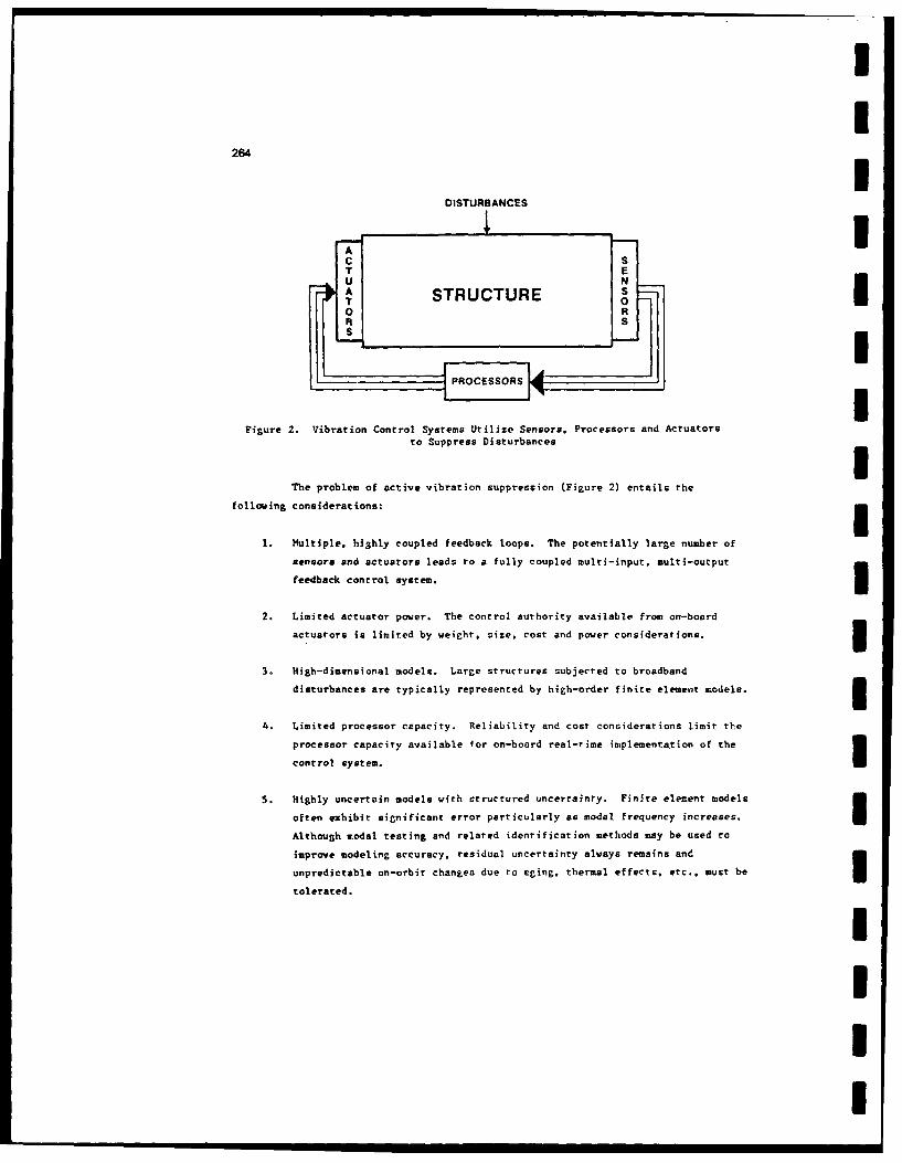
264

DISTURBANCES

U NSTASTRUCTURE 00 R

Figure 2. Vibration Control Systems Utilize Sensors. Processors and Actuatorsto Suppress Disturbances

The problem of active vibration suppression (Figure 2) entails the

following considerations: l1. Hultiple. highly coupled feedback loops. The potentially large number of

sensors and actuators leads to a fully coupled multi-input, multi-output

feedback control system.

2. Limited actuator power. The control authority available from on-board

actuators is limited by weight. size, cost and power considerations.

3. High-dimensional models. Large structures subjected to broadband

disturbances are typically represented by high-order finite element models.

4. Limited processor capacity. Reliability and cost considerations limit the

processor capacity available for on-board real-time implementation of the

control system.

5. Highly uncertain models with structured uncertainty. Finite element models Ioften exhibit significant error particularly as modal frequency increases.

Although modal testing and related identification methods may be used to

improve modeling accuracy, residual uncertainty always remains and

unpredictable on-orbit changes due to aging, thermal effects. etc.. must be Itolerated. I

IUI

1 265

6. Stringent performance requirements. Since active space structure control

is most relevant in precision applications, it can readily be expected that

performance specifications will be particularly stringent.

3 7. Design efficiency. Because of implementation complexity due to the

presence of multiple loops. high dimension, and high levels of uncertainty.

the control design approach should efficiently utilize both synthesis and3 analysis techniques (Figure 3).

i ANALYSIS

Figure 3. Control-System Design Must Efficiently Utilize BothSynthesis and Analysis Techniques

These considerations pose a considerable challenge to the state-of-the-art

in control-design methodologies. For example, the presence of multiple, coupled

feedback paths essentially precludes the effectiveness of single-loop designtechniques. The sheer number of loops, their interaction, and the need to address a

host of other issues render such methods inefficient and unwieldy.

In addition to the presence of multiple loops, the high dimensionality of

dynamic models places a severe burden on control-design methodologies. For example,

although LQG (linear-quadratic-Gaussian) design is applicable to multi-loop problems.

such controllers are of the same order as the structural model (Figures 4 and 5).

Thus LQG and similar high-order controllers can be expected to plece an unacceptable

computational burden on the real-time pro,essing capability. Hence it is notsurprising that a variety of techniques hav, heen ;-. ,sed to reduce the order of LQG

controllers. A comparison of several such metaods is given in [L.

All of the above difficulties are severely exacerbated by the fact that the

dynamic (i.e.. finite element) model upon which the control design is predicated may

be highly inaccurate in spite of extensive modal identification. Hence. applicable

control-design methodologies must account for modeling uncertainties by providing

robust (i.e.. insensitive) controllers. Furthermore, because of stringentIII

2663

HIGH-ORDER PLANT xeRn

i=Ax + Bu + UlCueR" ~y = CX+W yi

i= Acxc~+ Bcy DU = CX

FULL-ORDER CONTROLLER xccRn

STEADY-STATE PERFORMANCE CRITERION

J(ACBCCc) = rn EExTRjx + UTR 2U]

Figure 4. LQG Theory Addresses the Problem of Designing aQuadratically Optimal. Full-order Dynamic Compensator

FULL-ORDER CONTROLLER GAINS

As =A - Qi. -

C,=-R;'9~p

SEPARATED RICCATI EQUATIONS3

0o AO + OAT + V, _ Q .O (Kalman Filler)

0o ATP + PA. R1A - P:Y (Regulator)I

j=DRI8T ; =CTVlIC2 2

Figure 5. The Optimal Full-Order (LQG) Controller Is Determined by a

Pair of Separated Riccati Equationa

II

267

performance requirements, robust control design must avoid conservatism with respect

to modeling uncertainty which may unnecessarily degrade performance. A salient

example of conservatism is illustrated in Figure 6. If uncertainty in the modal

frequency is complexified in a transfer function setting, then the resulting pole

location uncertainty has the form of a disk. This disk. however, intersects the

right half plane in violation of energy dissipation. Hence one source of

conservatism is the inability to differentiate between physically distinct parameters

such as modal frequency and modal damping.

Im XRIGHT-HALF-PLANE

IMPOSSIBLE

01I Re

Re X

IIFigure 6. Corplexification of Real Parameters Hay Lead to Robustness Conservatism

Although classical methods are inappropriate for vibration control, a wide

variety of modern techniques are available. These include both multi-loop frequency-

domain methods and rime-domain techniques. A comprehensive review of such methods

will not be attempted here. Rather, we shall merely point out aspects of several

methods which motivate the philosophy of OPUS development.

As is well known, dynamic models can be transformed (at least in theory)

between the frequency and time domains. Significant differences arise, however, in

attempting to represent modeling errors. Specifically, model-error characterization

of a particular type, which is natural and tractable in one d'omain. may become

extremely cumbersome when transformed into the other domain. Fov example, consider a

state space model with parameter uncertainties arising in the system matrices

(A,B,C). Upon transforming to a frequency domain model G(s) = C(sI-A) IB the

parametric uncertainties may perturb the transfer function coefficients in aIII

I

complicated manner. A more natural measure of uncertainty for transfer functions has

been developed in (2] where system uncertainty in the frequency domain is modeled by

means of formed neighborhoods in the f-infinity topology. There are limitations with

this approach, however, in designing controllers for vibration suppression. For

example. as shown in Figure 6. complexification of real-parameter uncertainties such

as modal frequencies may yield unnecessary conservatism, while norm bounds often fail

to preserve the physical structure of parameter variations. A case in point is the

lightly damped oscillator. As shown in (A421. norm bounds predict stability over a

frequency range on the order of the damping while in fact the oscillator is Iunconditionally stable. Furthermore, with regard to processor throughput tradcoffs,

modern frequency-domain methods typically yield high-order controllers.

Although LQG addresses performance/actuator and performance/sensor

tradeoffs in a multi-loop setting, it fails to incorporate modeling uncertainty.

Thus it is not surprising, as shown in [3]. that LQG designs fail to possess

guaranteed gain margin. Since LQG designs lack such margins, attempts have been made

to apply frequency-domain techniques to improve their characteristics. One such

method, known as LQG/LTR (C4,5]) seeks to recover the gain margin of full-state- Ifeedback controllers. Specifically, full-state-feedback LQR controllers are

guaranteed to remain stable in the face of perturbations of the input matrix B of the

form aB where a[l1/2.-). As shown in 16,71. however, the full-state-feedback gain

margin fails to provide robustness with respect to perturbations which are not of Ithis form. For instance, the example given in [6] with B = [0 1] can be

destabilized for suitable performance weightings with perturbation B(C) = (E 11T for

arbitrarily small C in spite of the 6 dB margin. Furthermore, since LQG/LTR loop

shaping is based upon singular value norm bounds, treatment of physically meaningful

real parameter variations may lead to unnecessary conservatism. Several approaches

have been proposed for circumventing these difficulties (see. e.g.. [8]).

The importance of addressing the problem of structured uncertainty in

finite element models cannot be overemphasized. Structural characteristics such as

modal frequencies, damping ratios, and mode shapes appear explicitly in (A.BC)

state-space models as physically meaningful parameters. Uncertainty in mode shapes,

for example, which appear as columns of the B matrix, cannot in general be expected

to be of a multiplicative form in accordance with traditional gain-martin

specifications. This is precisely the problem illustrated by the example of (6]

discussed above. Furthermore, uncertainties in modal frequencies and damping ratios

must be carefully differentiated since, roughly speaking. moeal frequency

uncertainties affect only the imaginary part of the pole location while damping

uncertainty affects the real part. Although these and related observations

I

I

1 269

concerning uncertainty in the dynamic characteristics of lightly damped structures

my be self evident, they have remained largely unexploited in standard control-

design methods.

2. OPUS: New Machinery for Control-System Desitn

I In view of the ability of LQG theory to synthesize dynamic controllers for

multi-input, multi-output controllers, it is not surprising that LQG forms the basis

for a variety of structural control methods. However, as discussed previously, LQG

lacks the ability to address performance/processor and performance/robustness

tradeoffs. This situation has thus motivated the development of numerous variants of

LQG which entail additional procedures which attempt to remedy these defects. OPUS.

however, is distinctly different. Rather than append additional procedures to LQG

I design. OPUS extends LQG theory itself by generalizing the basic underlying

machinery.

j As shown in Figure 5. the basic machinery of LQG consists of a pair of

separated Riccati equations whose solutions serve to directly and explicitly

synthesize the gains of an optimal dynamic compensator. The contribution of OPUS is

to directly expand this machinery. The overall approach is illustrated in Figure 7

which portrays two distinct generalizations of the basic LQG machinery. As Figure 7

illustrates, these generalizations can be developed individually when either low-

order or robust controllers are desired. The appealing aspect of OPUS, however, is

the ability to extend LQG to address both problems simultaneously in a unified

manner.

U LOG2 RICCATI

(SEPARATED)LOW-ORDER

CONSTRAINT PARAMETERUNCERTAINTIES

OP us2RICCATI * YPNW2 RICCATI *2 LYAPUNOV

|COUPLEEDCV OOTIMAL PROJECTION) (COUPLED MY UNCERTAINTY TERMS)

PARAMETER LOW-ORDERUNCERTAINTIES CONSTRAINT

RICCATI - 2 LYAPUNOV(COUPLEO MY OPTIMAL PROJECTION

AND UNCERTAINTY TERMS)

I Figure 7. The Standard LQG Result Is Generalized by Both the Fixed-Order

Constraint and Modelin& of Parameter Uncertainties

II

I

II

270 3

In the following sections the generalizations depicted in Figure 7 will be

reviewed following the left branch. That is. the optimal projection approach to Ireduced-order controller design will first be discussed in Section 3 without

introducing plant uncertainties. In Section 4 the reduced-order constraint will be

retained while considering, in addition, uncertainties in the system model. In each

case the discussion will focus on the underlying ideas with a minimum of technical

detail.

Clearly, in order for a novel design methodology to be of pracrical value Iit must be compurationally tractable. Hence Section 5 will present an overview of

the current state of algorithm development for solving the OPUS design equations.

Finally, Section 6 will briefly summarize further OPUS generalizations of LQG theory Iwhich are relevant to structural control.

3. Extensions of LQG to Reduced-Order Dynamic Compensation

The simplest, most direct way to obtain optimal reduced-order controllers 3is to redevelop the standard LQG result in the presence of a constraint on controller

dimension (Figure 8). The mathematical technique required to do this is remarkably

straightforward. Specifically, the structure and order of the controller are fixed 1and the performance is optimized with respect to the controller gains. The resulting

necessary conditions obtained using Lagrange multipliers thus characterize the

optimal gains.

HIGH-ORDER PLANT xRn

i = Ax + Bu + w

u'Rm y xWD y.Rt

c Acic + Icy

u = Cc xc

LOW-ORDER CONTROLLER xc(R nc 3STEADY-STATE PERFORMANCE CRITERION

J(AC.Bc,Cc) = 11m E[xTRlx + uTR 2u]I-W IFigure 8. In Accordance With On-Board Processor Requirements, a Reduced-Order

Constraint Is Imposed on the Dimension of the Dynamic Compensator

I

I• i i l l I I I II I

II1 271

This parameter optimization approach as such is not new and was

investigated extensively in the 1970's. Typically. however, the optimality

conditions were found to be complex and unwieldy while offering little insight and

requiring gradient search methods for numerical solution.

One curious aspect of the parameter optimization literature is that no

attempt was made to actually use this direct method to rederive the LQC result

itself. Such an exercise, it may be surmised, might reveal hidden structure within

the optimality conditions which would shed light on the reduced-order case. Indeed.

such an approach led to the realization that sn oblique projection (idempotent

matrix) is the key to unlocking the unwieldy optimality conditions ([A7.A17]).

Although the result is mathematically straightforward, it is by no means obvious

since in the full-order (LQG) case the projection is the identity and hence not

3readily apparent.By exploiting the presence of the projection, the necessary conditions can

be transformed into a coupled system of four algebraic matrix equations consisting of

a pair of modified Riccati equations and a pair of modified Lyapunov equations

(Figure 9). The coupling is via the oblique projection T which appears in all four

equations and which is determined by the solutions Q and ; of the modified Lyapunov

equations. A satisfying feature of the optimality conditions is that in the full-

order case the projection becomes the identity, the modified Lyapunov equations drop

out. and, since 7 = 0. the modified Riccati equations specialize to the usual

separated Riccati equations of LQG theory. Since. furthermore. G = r = nxn identity.

the standard LQG gain expressions are recovered.

3 Although the modified Riccati equations specialize to the standard Riccari

equations in the full-order case, the modified Lyapunov equations have no counterpart

in the standard theory. The role of these equations can be understood by considering

the problem of optimal model reduction alone. For this problem the optimal reduced-

order model is characterized by a pair of coupled modified Lyapunov equations

(see [A22]). Thus the modified Lyapunov equations arising in the reduced-order

dynamic-compensation problem are directly analogous to the modified Lyapunov

equations arising in model reduction alone. The modified Lyapunov equations arising

in the control problem, howeyer. are intimately coupled with the modified Riccati

equations. Hence it cannot be expected that reduced-order control-design techniques

based upon LQG will generally yield optimal fixed-order controllers (Figure 10). It

is interesting to note that several such methods discussed in Rl] are based upon

balancing which was shown in [A22] to be suboptimal with respect to the quadratic

(least squares) optimality criterion.

II:

I.m s m m .a |B lm

II

272 3

REDUCED-ORDER CONTROLLER GAINS

Ac = I'(A-O Z-P)GT

Se = I'OCTV'1

CC = .R41 BTPGT I

COUPLED RICCATI/LYAPUNOV EQUATIONS

o = AO + OAT + V, - OO + IOIOrZT I0= A

TP * PA+R - P P + +y R P P r

0 = (A-XP)6 + O(A-!P)T + OZO - TO O iTo (A-03S)T P + P(A-07.) + PIP - FT!P

rank Q : rank P = rank 6P = nc

&P = GTMf' I'G = Inc

r =GTI:P(P) T = In -' 3SR-1 CTV-C

Figure 9. The Optimal Reduced-Order Compensator In Determined by aPair of Modified Riccati Equations and a Pair of Modified Lyapunov Equations

Coupled by the Oblique ProjectionT

IFIR UC TIN OPTIMAL "SPROJECTIONI

EQUATIONS I+

R CONTROLLER

FiJgure 10. The Optimal Projection Equations Provide a Direct Path toOptimal Reduced-Order Dynamic Compensators

III

........ G-I RElDUICTI IIION

II.1 273

In summary, the optimal projection equations for reduced-order dynamic

compensation comprise a direct extension of the basic LQG machinery to the reduced-

order control problem. The design equations, which reduce to the standard LQC result

in the full-order case, provide direct synthesis of optimal reduced-order controllers

in accordance with implementation constraints.

4. Extensions of LQG to Uncertain Hodelin

Two fundamental sources of error in modeling flexible structures are

truncated modes and parameter uncertainties. Since the optimal projection approach

permits the utilization of the full dynamics model, modal truncation can be largely

avoided. There remains. however, a tendency to truncate poorly known modes and thus

it is essential to incorporate a model of parameter uncertainty in both well-known

and poorly known components of the system. Hence the problem formulation of Figure 8

is now generalized in Figure 11 to include uncertain parameters Or. appearing in theA. B and C matrices. The parameter ori is assumed to lie within the interval (- -8]

Iin accordance with identification accuracy. Clearly. when uncer' ainty is absent.i.e.. when Ai. Bi. Ci = 0. the reduced-order design problem of Figure 8 is recovered.II

HIGH-ORDER, UNCERTAIN PLANT

@ Stochastic disturbance modela Deterministic parameter uncertainty model

Ia'iI <,5

UX= (AeZajAi)x + (8+Zoj~j)u +w

y (C+EoiCi)x + w 2

r n

LOW-ORDER CONTROLLERm Dynamic (strictly proper)* Static (constant gain)

•Dynamic/static (nonstrictly proper)

Figure 11. Robust Optimal Projection Design Is Based Upon aHybrid Uncertainty Model Involving a Deterministic Parameter Uncertainty Model

and a Stochastic Disturbance Model

III

274 5

A salient feature of the design model is that uncertainty is modeled in two

distinctly different ways. External uncertainty appearing as additive white noise is

modeled stochastically. Such a model appears appropriate for disturbances such as

coolant flow for which only power spectral data are available. On the other hand.

internal uncertainty appearing as parameter variations is modeled deterministically. 3Such a model appears appropriate for uncertainty arising from directly measurable

quantities such as mass and stiffness. Thus the overall uncertainty model is hybrid

in the sense that it utilizes both deterministic and stochastic characterizations of

uncertainty.

A natural performance measure which accounts for both types of uncertainty

characterization involves the usual LQG quadratic criterion averaged over the

disturbance statistics and then maximized over the uncertain parameters (Figure 12).

Hence this performance measure incorporates on the average and worst case aspects in

accordance with physical considerations.

PERFORMANCE CRITERION 3J(AcBc,Cc) Sup lim sup E [XTR 1 x + 2xTR12u + UTR2 u]

I t 1 I.

Wort- Steady- Average QuadraticC ase State

Over OverParameters Disturbance

StatisticsI

ROBUST PERFORMANCE PROBLEMMinimize J(Ac,BC,Cc) over the class of robustly

stabilizing controllers (AcBc,Cc) 1Figure 12. Performance Is Defined To Be Worst Case Over the Uncertain Parameters

and Average Over the Disturbance Statistics I

The result;ng Robust Performance Problem thus involves determining the

gains (Ac *Bc Cc) to minimize the performance J. The static gain Dc can also be 3included but will not be discussed here. Despite the apparent complexity of the

problem, remarkably simple techniques can be used. Specifically. first note that

after taking the expected value the performance J has the form 3J(A B C sup lim sup tr Q(t)R, (4.1)

c c (i t-),4

J(Ac.c.CII

II3 275

where "tr" denotes trace of a matrix. Q(t) is the covariance of the closed-loop

system, and fR is an augmented weighting matrix composed of RI. R12 and R2. The

covariance Q(t) satisfies the standard Lyapunov differential equation

IQ = (A+E. A.)Q + Q(A+ , A i)T + V. (4.2)

where A is the closed-loop dynamics. A. is composed of Ai. B. and Ci. and V is theIintensity of external disturbances for the closed-loop system including the plant and

measurement noise.

Two distinct approaches to this problem will be considered. The first

involves bounding the performance over the class of parameter uncertainties and then

choosing the gains to minimize the bound. Since bounding precedes control design

this approach is known as robust design via a priori performance bounds. The second

approach involves exploiting the nondestabilizing nature of structural systems via5 iweak subsystem interaction.

4.1 Robust Desipn Via A Priori Performance Bounds

3The key step in bounding the performance (4.1) is to replace (4.2) by a

modified Lyspunov differential equation of the form

_q + _2A + *(_q) + V. (4.3)

3 where the bound + satisfies the inequality

E:(A.+) T . (4.4)

I over the range of uncertain parameters C.. and for all candidate feedback gains. Notethat the inequality (4.4) is defined in the sense of nonnegative-definite matrices.5 Now rewrite (4.3) by appropriate addition and subtraction as

=(A+F A I )_q + 2(A. .A.) + +(g) - E q + V. (4.5)

I Now subtract (4.2) from (4.5) to obtain

|T_- Q = (A+o oA i)(g-Q) + (_q-Q)(A+Ia'-i Ai)T + 4(_) - , ,(A1 ,+ ). (4.6)

II1

I

276 3

Since by (4.4) the term

is nonnegative definite, it follows immediately that I

(4.8)

over the class of uncertain parameters. Thus the performance (4.1) can be bounded by I

J(A Bc.C c ) ( J(A *Bc.C ) lir tr gR. (4.9)

It-)IThe auxiliary cost J is thus guaranteed to bound the actual cost J. This leads to

the Auxiliary Minimization Problem: Minimize the auxiliary cost I over the

controller gains. The advantage of this approach is that necessary conditions for

the Auxiliary Minimization Problem effectively serve as sufficient conditions for

robust performance in the original problem. Since the bounding step precedes the

optimization procedure, this approach is referred to as robust design via a priori Uperformance bounds. This procedure is philosophically similar to guaranteed cost

control ((9.10]). Note that since bounding precedes optimization, the bound (4.4)

must hold for all gains since the optimal gains are yet to be determined.

To obtain sufficient conditions for robust stability, the bounding function

must be specified. Since the ordering of nonnegative-definite matrices appearing lin (4.4) is not a total ordering, a unique lowest bound should not be expected.

Furthermore. each differentiable bound leads to a fundamental extension of the

optimal projection equations and thus of the basic LQG machinery. In work thus far. 5two bounds have been extensively investigated. Only one bound, the right

shift/multiplicative white noise bound, will be discussed here. The structured

stability radius bound introduced in (11.12] is discussed in [A43]. 3The right shift/multiplicative whire noise bound investigated in [A29.A41]

is given by n

4(9) = ( +(ig (4.10)

where a. 0 are arbitrary scalars. Note that this bound consists of two distinct Iparts which must appear in an appropriate ratio. The first term a9R arises naturally

when an exponential time weighting e is included in the performance measure. As

is well known ([13]) this leads to a prescribed uniform stability margin for the

III

3277

closed-loop system (Figure 13). A uniform atability margin, no matter how large,

however, does not guarantee robustness with respect to arbitrary parametervariations. The complementary second term -il T. is crucial in this regard.

iAX -01 =(A+al)x,a>0Im

IX

IXAPPLY CONTROL-DESIGN TECHNIQUES

TO RIGHT-SHIFTED OPEN-LOOP SYSTEMI UNIFORM STABILITY MARGIN

(Anderson and Moore, 1969)

3 Figure 13. Open-Loop Right-Shifted Dynamics Arising From Exponential Cost WeightingLead to a Uniform Closed-Loop Stability Margin

Although terms of the form A i2A are unfamiliar in robust control design.they arise naturally in stochastic differential equations with multiplicative white

noise. That is, if the uncertain parameters o are repleced by white noise processes

entering multiplicatively rather than addirively, then the covariance equation for Q

automatically includes terms of the form AiQA. The literature on systems with

multiplicative white noise is quite extensive; see (A38] for references. It should

be sVressed. however, that for our purposes the multiplicative white noise model is

not interpreted literally as having physical significance. Rather. miulriplicarive

white noise can be thought of as a useful desirn model which correctly captures the

impsct of uncertainty on the performance functional via the state covariance.

Furthermore, just as the right shift term alone does not guarantee robustness.

neither does the multiplicative white noise term. Both terms must appear

simultaneously. Roughly speaking, since multiplicative white noise disturbs the

plant though uncertain parameters, the closed-loop system is automatically

desensitized to actual parameter variations.IIIU

II

278

After incorporating the right chifr/mulriplicarive white noise bound (4.10)

into (4.3) to obtain a bound J for the performance, the optimal projection equations

can be rederived following exactly The same parameter optimization procedure

discuased in Section 3. Again, the mathematics required is but a straightforward

application of Lagrange multipliers. The additional bounding terms are carried

through the derivation to yield a direct generalization of the optimal projection

equations shown in Figure 14 with gains given in Figure 15.

s+ v1 +(AI4R 2sPs)Q(+.t+R 2ss) ' + V2 kr V1TTO~ Q O AT S -I As 2s T) - -1V SO I~ I 2s S

O=AT.P+PA5 4 TPA +R+ (QS-1 TA -1 TJR -1P I-TITR-1 11,r

A R1 (.AQsV 2S) P(A-QsV 2s') S $"2ss + i s 2s sri

-1 A A -1 T -1 TT(As-BsR 2 P)Q + (As-BSR2sP) + QsV2 ' 1'. 2s s1

21Cs)TA A -1 P-R 21sI'_ TT R

V2SCS)r P + (S5R2 s

0 (As-1sV ' PI s V 2SC S) rs) 5 S

Figure 14. The Robustified Optimal Projection Design Equations Account for Both 1Reduced-Order Dynamic Compensation and Parametric Uncertainty

GAINS3AC=1(A. -1 p - T

Ac =I'(A-BsR 2s s-QsV2s Cs)GT

-II8C= I Qs 2s

Cc = R'lPsGT2s NOTATION IOP :GTMr. PG T = Inc ( r: GTp r2)

AQAT = AiQATQ AQ = !AiQB 1 , etc.i=1 " I1A A

R2S R2 + * T(P+P)B V2s V2 + ¢(Q+O)CT

AAOCT + A)T B T + T (PP.OC +AV12 C ~ 12 8 ~~)

Figure 15. The OPUS Controller Cains Are Explicitly Characterized as aDirect Generalization of the Classical LQG Gains I

II

3 279

The robustified optimal projection equations comprise a system of four

matrix equations coupled by both the optimal projection and uncertainty terms. When

the uncertainty terms are absent, the optimal projection equations of Figure 9 are

immediately recovered. On the other hand, if the order of the controller is set

equal to the order of the plant, then all terms involving T, can be deleted.

However, in this case the modified Lyapunov equations do not drop out since Q and P

still appear in the modified Riccari equations. Hence the basic machinery of LQC is

again extended to include a pair of Lyapunov equations coupled to a generalization of

the standard LQG equations. It is interesting to note that a related result in the

context of multiplicative noise also appeared in the Soviet literature ([14]). It

should also be pointed out that although the modified Lyapunov equations arising in

the reduced-order control-design problem have analogues in model reduction, the

modifi Lyapunov equations appearing in the full-order robuctified equations

represent new machinery not anticipated in robustness theories. Hence using

Sstraightforward mathematical techniques, the basic LQC machinery has again beenextended in novel directions.

5 1 Solving the design equations shown in Figures 14 and 15 yields controllers

with guaranteed levels of robustness. The actual robustness levels may. however, be

larger than specified by a iriori bounds. Thus, to achnve desired robustificationIlevels for the uncertainty structure specified by the a priori bounds, the designprocedure may be utilized within an iterative synthesis/analysis procedure

(Figure 16).

SYNTHESIS

CONTRUCT~-,DESIGN CONTROLLER_ STABILITYORANDE

BONS TO MINIMIZE BOUNDS GURRANED

STABILITY AND |PERFORMANCE~ROBUSTNESS

ANALYSIS

Figure 16. Optimal Projection/Guaranteed Cost Control Provides

Direct Synthesis of Robust Dynamic Compensators

4.2 Robust Design Via Weak Subsystem Interaction

3 The mechanism by which LQC was robustified in Section 4.1 nvolved bounding

the performance over the class of narameter uncertainties and then derermining

optimal controller gains for the performance bound. As discussed in Section 2.I

IU

I

280

however. flexible structures possess special properties which may, in addition, be

exploited to achieve robustness. Specifically. aside from rigid-body modes, energy Udissipation implies that mechanical structures are open-loop stable regardless of the

level of uncertainty. That is. flexible structures possess only nondesrabilizinz

uncertainties. Hence. in the closed loop. a given controller may or may not render a 5particular uncertainty destabilizing. A priori bounds on controller performance

must, however, be valid for all gains since bounding precedes optimization. Hence. a

priori bounding may in certain cases fail to exploir nondestabilizing uncertainties. 3A familiar example of a nondestabilizing uncertainty involves uncertain

modal frequencies. Such an uncertainty will not, of course, destabilize an

uncontrolled (open-loop) structure. If particular modal frequencies are poorly known 1then it is clearly advisable to avoid applying high authority control. Hence. rather

than the right-shift approach of Figure 13, it appears advantageous (although, at

first. counterintuitive) to utilize just the opposite, namely, a left shift m(Figure 17). Furthermore, in view of the fact that uncertainty usually increases

with modal frequency (Figure 18). a variable left shift appesr . to be more

appropriate than a uniform left shift. By left-shifting high-frequency poorly known

modes, the control-system design procedure applies correspondingly reduced authority

to modes "perceived" as highly damped. Hence the variable left shift can be roughly

thought of as a device for achieving suitable authority rolloff. As will be seen,

however, the underlying robustification mechanism, namely, weak subsystem interaction,

is far more subtle than the approach of classical rolloff techniques. It is also

interesting to note that the weak subsystem interaction approach to robustness is

entirely distinct from classical robustness approaches which utilize high loop gain

to reduce sensitivity.

p=Ax + =(A+ - A2 )X

2 J

LARGE OPEN-LOOP SHIFTIN HIGH-FREQUENCY REGION

LOW CLOSED-LOOP AUTHORITY

_ _ _ ) SMALL OPEN-LOOP SHIFT 3IN LOW-FREQUENCY REGION- HIGH CLOSED-LOOP AUTHORITY

- Re IFigure 17. A Variable Left Shift Exploits Open-Loop Nondestabilizing Uncertainties U

II

II

I 281

3 MODAL FREOUENCY

I J _ __t

COHERENT MODES INCOHERENT MODES

(SUOMI C6IliOn) (Weak Correlation)

3 hi yCentf ral Low-Auathr CanuoI

Figure 18. Hodal Uncertainty Generally Increases With Frequency

I A variable left shift can readily be introduced into the robustified

optimal projection design equations by replacing A by

A. = A+ , ( !4.1)

where A. denotes the structure of modal frequency uncertainty (Figure 19). Most

interestingly, such a modification of the dynamics matrix arises naturally from a

multiplicative white noise model defined not in the usual Ito sense but rather in the

3sense of Stratonovich. Thus, as in the a priori bounding approach, a stochastic

.071 017"11 0 " 0r - -

S+ II0 1-,' 1 1L "

r --

c: A +/2!A 2 4 io Variable Left Shift

Figure 19. For rodal Systems With Frequency Uncertainty

the $tratonovich Correction Corresponds to a Variable Left Shift

III

I282 1

model serves to suggest a mechanism for robustification (Figure 20). Again it is

important to stress that the multiplicative white noise model is not interpreted

literally as having physical significance, but rather can be thought of as a useful

design model which correctly captures the impact of uncertainty on the performance

functional via the state covariance. 3ROBUSTNESS BOUNDS

I IOUADRATIC LYAPUNOV FUNCTION MAJORANT LYAPUNOV FUNCTION

ITO NOISE MODEL STRATONOVICH NOISE MODEL J

STOCHASTIC UNCERTAINTY MODELS 3Figure 20. Stochastic Models and Robustness Bounds Are Fundamentally Related

In earlier work the Stratonovich dynamics model was justified by means of I

the minimum information/maximum entropy approach ([Al-A15). A central result of the

maximum. entropy approach is that the high aurhority/low authority transition of a

vibration control system from well-known low-frequency sodes to poorly known high- Mfrequency modes (Figure 18) is directly reflected in the structure of the state

covariance matrix (Figure 21). A full-state feedback design applied to a simply 3I

.. .. :Okk -0

R0 Qnn

COHERENT = NCOHERENT

(WELL-KNOWN MODES) (POORLY KNOWN MODES)

INFORMATION REGIMES 1Figure 21. Frequency Uncertainties in the Stratonovich Model Lead to

Suppressed Cross Correlation in the Steady-State Covariance III

IU

1 283

supported beam illustrates this point (Figure 22). By assuming that uncertainty in

modal frequencies increases linearly with frequency, the structure of the covariance

matrix leads directly to the control gains illustrated in Figure 23. Note that in

the high-frequency region the position gains are essentially zero and thus the

control law approaches positive-real energy dissipative rate feedback. This, of

course, is precisely the type of structural controller expected in the presence of

poor modeling information. Of course, any effective control-design theory for active

vibration suppression in flexible structures should produce energy dissipative

controllers when structural modeling information is highly uncertain.

N EONOIMENSIONAL EOUATIONS

OF MOrOn (i Z .21

* 1E55c STATE-WIGH551)5* UNCERTAINTIES IN OPEO-LOOP

FRLOUENCICS

3 T-_ , ('Ki ).I

X = STANDARD OfVtATIOR

1, 2!43 OF K* MOOE FREOUENCY

i SIMPlE UNCERTAINTY MODEL

SIMILYSUPPORTEO BEAM WITH FORCE ACTUATOR OWN

rUEL.-STATE IFORACK

Figure 22. The Effects of Frequency Uncertainties Can Be Illustrated5for a One-Dimensional Beam With Idealized Full-State Feedback

To carry out robustified optimal projection design in the presence of left-

shifted open-loop dynamics, it is only necessary to utilize the left-shifted dynamicsI!matrix (4.11) in place of the right-shifted matrix. All of the robustified optimal

projection machinery, including gain expressions, can be utilized directly. It is

also important to stress that the left shift must be used in conjunction with terms

of the form AQA T

One explanation for the mechanism by which robustificarion is achieved is

illustrated in Figure 24. By left shifting the open-loop dynamics within the design

process, the compensator poles are similarly left-shifted. Thus the compensator

poles are effectively moved further into the left half plane away from the actual

plant poles. Since the interaction between compensator and plant poles is weakened,

the closed-loop system is correspondingly robustified with respect to uncertainties

in the plant pole locations. A sensitivity analysis of this mechanism utilizing a

uniform left shift in the context of LQG design is given in [151.

III

II

284

07: (Ions. P- or= 0 1)i

tO -

DS VfLOCIT GAINi

POSITIN CAlM

I s ,9 is 26 25 30 3 . s 0

NIGN.*UUII1RI?Y IDIW.AUTHORITY RfrION

TRANSITION iREGION11

A 0011ST[!0P1!CT Of ISULT OF STRATNOVICH MOBt L

Figure 23. The Maximum Entropy Controller Approaches Rate Feedback in theLimit of Poor Modeling Information (Hieh Uncertainty)

A+ ¢ c• qc[A tAc.] [ A .]0 [180c 0~ce

I = 1 -*LOG Plant/Compensator Subsystem InteractionsSubsystems

0 7 co 1

If

LOG puts compensator Wider separationpoles near plant poles C€ 0(r2) shill (week Interaction)1

CI OW() shill (strong Interlton) __.. ... __

c:: Decreased sensitivity toplant verlti ons

Figure 24. The Straronovich Variable Left-Shift Model Effectively Places theCompensator Poles Further Into the Left Half Plane Where

Plant/Compensator Interaction In Weakened

II

3 285

As discussed above, the left-shift approach exploits open-loop

nondestabilizing uncertainties and thus cannot operate through a priori bounding.

Thus the actual level of robustification achieved from the robustified optimal

projection equations for a given level of uncertainty modeling cannot be predicted a

priori. i.e.. in advance of control design. Indeed. thia situation is to be expected

when nondestabilizing uncertainties are exploited in a nonconservative design theory.

Thus a suitable robust analysis technique is required for nonconservatively

determining the robustification of the closed-loop system with respect to open-loop

nondestabilizing uncertainties.

A suitable robustness analysis technique, known as majorant Lyapunovanalysis, has indeed been developed ([A42]). Essentially, this technique employs a

new type of Lyapunov function for assessing robustness due to weak subsystem

interaction. The underlying machinery consists of the block-norm matrix which is a

nonnegative matrix each of whose elements is the norm of a block of a suitably

partitioned matrix (Figure 25). A matrix which bounds the block-norm matrix in the

sense of nonnegative matrices. i.e.. element by element, is known as a majorant.3ajorants were introduced in (161 and were applied to stability analysis of

integration algorithms for ODE's in [17].

I (Ostrowski, 1961; Dahlquist, 1983)

1A [M1 M12-- 1

M= M21 M2

I %

[IIMiII 11M 12 11---I I[M2111 IIM211

I"

3NONNEGATIVE CONE ORDERING

I Figure 25. The Matrix Majorant Is a Bound for the Matrix Block Norm.i.e., the Nonnegative Hatrix Each of Whose Elsments Is the Norm of the

Corresponding Block of a Given Matrix

IIIU

2861

To apply majorants to dynamical systems, the model is written in the form

shown in Figure 26. The matrix A is block diagonal and consists of subsystem

dynamics. The subsystem interactions represented by the partitioned matrix G are

assumed to be uncertain. By suitable manipulation, uncertainties in the diagonal

blocks ot A can also be captured by G. By assuming that the spectral norm (largest

singular value) of the blocks of G satisfy given bounds, the covariance block-norm

inequality is obtained (Figure 27). This inequality is interpreted in the sense of

nonnegative matrices, i.e., element-by-element, and * denotes the Hadamard (element-

by-element) product.

:(A+ G)x +w 0(A G)Q +.Q(A + G)T+V

G o 2--1

A A0 A2] G 1

I * IJ I

Known Subsystem DynamISc Uncrlsnr Subsystem Inli :lions

V[VV 11 V1- --n 021 012 -

Nolte Intensily Slate Covsrlpnce

Figure 26. The Large-Scale System Model Involves Known Local Dynamicsand Uncertain Interactions

x = (A + G)+w J E[xTRx It

OrQR

0 = (A + G)0 + O(A + G)T + V A: I(A 0 Aj)I

,,V1,, 11V21IF--- [,,O.,,F ,,12,IIFV= IIV21i1F IIV211" Qs IIO,1IIF II 2 lF 1 1I N.

](G211 0

"Q <--<9Q +QgT +VIL

Figure 27. The Block-Norm Matrix of the State Covarlance Satisfies a

Lyapunov-Type Inequality Involving Nonnegative Matricea

II1

, i i i I II II

3 287

To achieve robustness, the covariance block-norm inequality is replaced by

the smajorant Lyapunov equation (Figure 28). The solution of the majorant Lyapunov

equation provides a bound (majorant) for the block norm of the covariance thereby

guaranteeing both robust stability and performance.

MAJORANT LYAPUNOV EQUATION

"aQ=SQ+QST + V

U(Gij) <- Cjj

I'D

n Robust Stability

s Robust Performance

3 Figure 28. The Corresponding Nonnegative Matrix Equation Yields a Hajorantfor the State Covariance and Hence Robust Stability and Performance

It is interesting to note that numerical solution of the majorant Lyapunov

equation requires no new techniques. Utilizing properties of H matrices, the

solution can be obtained monotonically by means of a straightforward iterative3 technique (Figure 29).

MLE has a unique solution ill (QK, K=O, 1 ... , -1 where:

0 0

QK+1 V I (, K + (\K,(T +

I (01mn /

converges. II so, then:

( irn QK

rJ - JO2S2 (tr PK)(s'Q))KK

K=1

T ^ +,(0 = A KP K P PK AK + RK)

figure 29. By Exploiting the Properties of --Matrices.

the ajorant Lyapunov Equation Can Be Solved Monotonically by Means of aSimple Iterative TechniqueI

IU

I

I

An illustrative application of the majorant Lyapunov equation involves

lightly damped subsystems (Figure 30). As shown in [A421 (and expected intuitively).

robustness with respect to uncertain subsystem interaction is proportional to the

frequency separation between the subsystems. The ability to capture this

robustification mechanism is a unique feature of the majorant Lyapunov function not

available from quadratic (i.e.. scalar) Lyapunov functions or vector Lyapunov

functions ([18.191). I,

Majorant Lyapunov Equation Bound- v 1(2v)2 + (w1-w2) 2 3Figure 30. Robustness Bounds for Uncertain Coupling in Modal Systems

Are Proportional to the Frequency Separation Between Subsystems

The next step in the majorant development involves a hierarchy of finer and Ifiner robustness bounds which account for higher order subsystem interactions. e.g.,

the interaction between the ith and jth subsystems via the kth subsystem. The second

member of the hierarchy (Figure 31) provides robustness guarantees with respect to

frequency uncertainties. The interesting aspect of this robustness test is the fact

that the performance bound is characterized precisely by a Stratonovich model. Hence

the Stratanovich model can be viewed as an approximation to a robustness bound, while

exploiting the Stratonovich/majorant relationship leads to a natural

synthesis/analysis scheme (Figure 32) which nonconservatively exploits open-loop

nondestabilizing uncertainties. 3

I111

1 289

SYNTHESISI UTILIZE STRATONOVICH MODELTO EXPLOIT NONDESTABILIZING

OPEN-LOOP UNCERTAINTIES

UTILIZE MAJORANT LYAPUNOVEQUATION TO CHECK ROBUSTNESS WITH

RESPECT TO CLOSED-LOOP NONDESTABILIZING

SUBSYSTEM INTERACTIONI ANALYSISStratonovich synthesis =approximation to majorant analysis

I Figure 31. The Stratonovich Synthesis Model Provides a first Approximation to the

IaoatAalssBud

Second member of the hierarchy:

r I

J - tr[dR] f:- 21. (tr PK)(b<KQ,>)KKK=1

o AO + OAT + II^]+v0O=AT^ + A + 1t[P] +R

I~C whre ott-diagonal part of Q13 Ja.1 = Stratonovich model operator

Tighter bound-incorporates more Information on A and 6aPredicts stability when (A + AT) stable, G= G

a "'Nominal" performance, tr (OR], given by Stratonovich model5 Figure 32. The Refined ?4jorant Bound incorporates a Stratonovich Covariance Model

I

290

5. Numerical Algorithms and Examples

Practical design of controllers is only possible when efficient, reliable Ialgorithms are available. Indeed, the optimal projection equations are readily

solvable and have been applied to a wide variety of examples. Numerical results

appear In [A3-A6,A.AI1.A12.A14-AI6,AI8,Al9,A21-A24,A26-A28.A30-A33.A39.A42.A44.A461.

Two distinctly different algorithms have been developed thus far. namely, an

iterative method and a homotopy algorit. 3The iterative method, developed in [A14oA16,A441 and further studied in

[20.211. is outlined in Figure 33. The nice feature of this approach is that only

a standard LQG software package is required for its implementation. The basic

motivation for the method is the observation that the main source of coupling is

via the terms involving rI. The coupling is absent, of course, when r is the

identity. i.e.. LQG. Note also that the terms involving 71 are small when R2 and

V2 are large. i.e.. when control cost is high and the measurement noise is isignificant. This case, which yields low-authority controllers, is approximately

characterized by decoupled control-design and controller-reduction operations.

Thus it is not surprising that LQG reduction techniques are most successful when

controller authority is low.

Since the TL terms occasion the greatest difficulty, it appears

advantageous to bring them into play gradually. This can be accomplished by fixing

T after each iteration to yield updated values of Q. P. Q and P. Furthermore. t is

introduced gradually by means of a to reduce its rank. 3The crucial step of the algorithm concerns the construction of the

projection r from the pseudogramians Q and P. Specifically. 7 can be characterized

(see [A22]) as the sum of eigenprojections of QP. where each choice of

eigenprojections may correspond to a local extremal. However. the necessary

conditions do not specify whic h eigenprojections are to be selected for obtaining a

particular local solution. Nevertheless, there do exist useful methods for

constructing 7. For example, component-cost decomposition methods ([22]) when

applied within the optimal projection framework often permit efficient identification

of the global optimum.I

Although the iterative method is convenient to use because it utilizes

readily available software, it is suboptimal in the sense that it does not fully

exploit the structure of the equations. Specifically. while the iterative method

addresses a system of four nxn matrix equations, careful analysis reveals that

because of the rank deficient) of the projection the problem can be recast as four

ncxn equations. Hence. when nc is much smaller than n. which is clearly the most ICI

III

U 291

IDP7 .P.0 ~

0= ~ Tp +A.,~,O O( 5A~F) QVr +T pT

0 (AS-Q,V21C, P (A.Q C,) *Fe ss R2 '

I UPDATE 7BALANCE: 1i -41A2 I

WT 4, -1 j ,- = AIA : IAG(A, . a)7- WIs 01 4 "

1 Ai >Ai,1

=: DIAGI ,A,, A.)

COMPUTE Q " V 2 F I 32 Ap,. AO,

BASED ON 0. P. 0

figure 33. The Iterative Hethod for Solving the Robustified OPUS Design

Equations Requires Only an LQG Software Package and

Involves Refinement of tbe Optimal Projection r

292I

desirable case for practical implementation. there exists considerable opportunity

for increased computational efficiency. Furthermore. and most satisfying, the

computational complexity decreases with n as is intuitively expected below that

required by LQG design. Hence the optimal projection approach has computational

complexity less than LQG reduction methods for which LQG is but the first step.

S. Richter ([23.A46]) has developed a homotopy algorithm which fully

exploits this crucial structure. Numerical experiments thus far have shown that

considerable computational savings can be achieved over the iterative method. IFurthermore. by applying topological degree theory to investigate the branches and

character of the local extremals. it can be shown that the maximum number of possible

extremals is

(min(n.m.2))

if nc( min(n.m.) or I otherwise. Hence in most practical cases the equations

support a relatively small number of solutions.

Both the iterative method and the homotopy algorithm have been applied to a

design problem involving an 8th-order flexible structure originally due to D. Enna

and considered in [I]. Specifically. a variety of LQG reduction methods are compared Iin [1) for a range of controller authorities. These methods include:

I. Enna: This method is a freqgency-weighted, balanced realization technique Iappiicable to either model or controller reduction.

2. Glover: This method utilizes the theory of Hankel norm optimal 3approximation for controller reduction,

3. Davis and Skelton: This is a modification of compensator reduction via 3balancing which addresses the case of unstable controllers.

4. Yousuff and Skelton: This is a further modification of balancing for 5handling stable or unstable controllers.

5. Liu and Anderson: In place of using a balanced approximation of the

compensator transfer functJc,; directly, this method approximates the Icomponent parts of a fractional representation of the compensator. I

I'I

293

All of the above methods proceed by first obtaining the full-order LQG

compensator design for a high-order state-space model and then reducing the dimension

of the resulting LQG compensator.

Figure 34 summarizes the results reported in (1J for the above LQG

reduction methods along with results obtained using the iterative method for solving

the optimal projection equations. Here q2 is a scale factor for the plant

disturbance noise affecting controller authority. Clearly. LQG reduction methods

experience increasing difficulty as authority increases. i.e.. as the r, terms become

increasingly more important in coupling the control and reduction operations. for

the low authority cases, the optimal projection calculations, which were performed on

a Harris H800 minicomputer, appeared to incur roughly the same computational burden

as the LQG reduction methods. Although the optimal projection computational burden

increases with authority. comparison with the LQG reduction methods is not meaningful

because of the difficulty experienced by these methods in achieving closed-loop

stability. See [A441 for further details and for comparisons involving transient

response.

The homotopy algorithm was also applied to the example considered in (1.

One of the main goals of the development effort was to extend the range of

disturbance intensity or. equivalently, observer bandwidth. out beyond q2 = 2000. To

this end. second-order (nc = 2) controllers were obtained with relatively little

computation for q2 = 10.000. 100.000 and 1.000.000. In addition, the performance of

each reduced-order controller was within 25% of LQG. These cases can surely be

expected to present a nontrivial challenge to both the LQG reduction methods and the

iterative optimal projection method.

Numerical solution of the robustifled optimal projection equations has been

carried out for several examples. For illustrative purposes a 2x2 example was

considered in CA261 and the results illustrated in Figure 35 indicate performance/

robustness tradeoffs possible. The variable left-shift technique was applied in

[Alg] to the NASA SCOLE problem with frequency uncertainties. The robustness of LQG

and two robustified designs is shown in Figure 36. The plots illustrate the

a Idegradation in performance due to simultaneous perturbation of all modal frequencies.

Note that LQG is rendered unstable by +5% frequency perturbation while a high-

authority robustifled design improves this region to +8Z. The low-authority design

increases this region significantly while sacrificing 6% nominal performance.

A

* I

294

method 2 0.01 0.1 1 10 100 1000 2000

7 S S S S S S S6 S S S S S S S

Enna 5 S S S S S S S4 S S S S S S U I3 S S S S S S S2 S S S S U U U

7 S S S S S U S

6 S S S S U U U UGlover 5 S S S S U U U

4 S S S S U U U3 S S U S U U U2 S U S U S U U

7 S U U S S S S6 S S S S S S S

Davis& 5 S U S S S U USkelton 4 S S U S S U U

3 U U U U U U U2 S U S U U U U

7 S S S S U U U

6 S S S S U U UYousuff & 5 S S S U U U U

Skelton 4 S S S U U U U3 S U U U U U U2 S S S U U U U

7 , , S . S S7 3 S S S S S U6 3 S S s S S S U

Liu& 5 3 S S S S S SAnderson 4 3 S S S S S S

3 S S S S S U U2 S S S S S S S

7 S S S S S S S6 S S S S S S S U

Opt imal 5 8 S S S S S S

Projection 4 S S S S S S S3 S S S S S S S2 S S S S S S S

S - The closed-loop system Is stableU - The closed-loop system is unstable

figure 34. The Optimal Projection Approach Was Compared toSeveral LQG Reduction Techniques Over a Range of Controller

Authorities for an Example of Enns

III

• !

I 295

Il. ,..$b . b 1-.0pG

3 250

IS

3o b' (Actual Value)

Figure 35. The Robuatified Optimal Projection Equations ProvideRlobustness/Performiance Tradeoffs for a Highly Sensitive Nominal LQG Desigt.

2961

RMS LOS ERROR DEGRADATION M~

LOGDESIGN DESIGN fl

351

30

251

23

IsI

-20 -15 -10 5 5 I i s1 23

#400AL FREQUENCY PERTURBATID14 M%

figure 36. The Stratonovich Model Robustifiea theILQG Dosi~ri for the NASA SCOLE Model with

Uncertain Modal Frequencies

I

1 297

6. Additional Extensions

The robustified optimal projection design machinery has been further

extended to encompass a larger number of design cases arising in practical

application. Here we merely list the extensions:

I. Discrete-time and sampled-data controllers ((A28.A30.A34.A35]).

1 2. Decentralized controllers ([A39)).

1 3. Nonstrictly proper controllers ((#371).

4. Distributed parameter systems ([A251).

U 7. Concludin& Remarks

The machinery provided by OPUS for designing active controllers for

flexible structures has been reviewed. The basic machinery is a system of coupled

Riccati and Lyapunov equations which directly generalize the classical LQG result to

include both a constraint on controller order and a model of parameter uncertainty.

The overall approach thus encompasses all major design tradeoffs arising in

vibration-suppression applications. Substantial numerical experience has been gained

through an Iterative method requiring only an LQG software package and. more

recently, by means of a highly efficient homotopy algorithm developed by S. Richter.

The overall approach opens the door for effective design of implementable controllers3 for large precision space structures.

Acknovledgment. We wish to thank Ms. Jill M. Straehla for the excellent3 preparation of this paper.

IIIIII1

298

General References

1. Y. Liu and B. D. 0. Anderson. "Controller Reduction Via Stable Factorizationand Balancing." nt. .j. Contr. Vol. 44. pp. 507-531. 1986.

2. G. Zames, "Feedback and Optimal Sensitivity: Model Reference Transformations.Multiplicative Seminorms. and Approximate Inverses." IEEE Trans. Autom.Contr.. Vol. AC-26. pp. 301-320. 1981.

3. J. C. Doyle. "Guaranteed Margins for LQG Regulators," IEEE Trans. Autom.

Contr.. Vol. AC-23. pp. 756-757. 1978.

4. J. C. Doyle and G. Stein. "Nultivariable Feedback Design: Concepts for aClassical/Modern Synthesis." IEEE Trans. Autom. Contr.. Vol. AC-26. pp. 4-16.1981.

5. G. Stein and M. Athans, "The LQG/LTR Procedure for Multivariable FeedbackControl Design." IEEE Trans. Autom. Contr.. Vol. AC-32. pp. 105-114. 1987.

6. E. Soroka and U. Shaked. "On the Robustness of LQ Regulators." IEEE Trans.Autom. Contr.. Vol. AC-29. pp. 664-665, 1984.

7. U. Shaked and E. Soroka. "On the Stability Robustness of the Continuous-TimeLQG Optimal Control." IEEE Trans. Autom. Contr.. Vol. AC-30. 1039-1043.

8. J. C. Doyle, "Analysis of Feedback Systems with Structured Uncertainties." IEEProc.. Vol. 129. pp. 242-250. 1982.

9. S. S. L. Chang and T. K. C. Peng. "Adaptive Guaranteed Cost Control of Systemswith Uncertain Parameters." IEEE Trans. Autom. Conrr.. Vol. AC-17. Ipp. 474-483. 1972.

10. A. Vinkler and L. J. Wood. "Multistep Guaranteed Cost Control of LinearSystems with Uncertain Parameters." J. Guid. Contr.. Vol. 2. pp. 449-456.1979.

11. 1. R. Petersen and C. V. Hollot. "A Riccati Equation Approach to theStabilization of Uncertain Systems." Automatics, Vol. 22. pp. 433-448. 1986.

12. D. Hinricbaen and A. J. Pritchard. "Stability Radius for StructuredPerturbations and the Algebraic Riccati Equation." Sys. Contr. Lett.. Vol. 8.pp. 105-113. 1986.

13. B. D. 0. Anderson and J. B. Moore. Linear Optimal Control. Prentice-Hall. IEnglewood Cliffs. NJ. 1970.

14. G. N. Milatein. "Design of Stabilizing Controller with Incomplete State Datafor Linear Stochastic System with Multiplicarive Noise." Autom. Remote Contr...

Vol. 43. pp. 653-659, 1982.

15. G. A. Adamian and J. S. Gibson. "Sensitivity of Closed-Loop Eigenvalues andRobustness." preprint.

16. A. M. Ostrowski. "On Some Metrical Properties of Operator Matrices andMatrices Partitioned into Blocks." J. Math. Anal. Appl.. Vol. 2. pp. 161-209.1961.

17. G. Dahlquist. "On Matrix Majorants and Minorants. with Applications to

Differential Equations." Lin. Alg. Appl.. Vol. 52/53. pp. 199-216. 1983.

UII

I

I29918. D. D. Siljak. Large-Scale Dynamic Systems. Elsevier/North-Holland. 1978.

19. M. Ikeda and D. D. Siljsk. "Generalized Decompositions of Dynamic Systems andVector Lyapunov functions." IEEE Trans. Autom, Contr.. Vol. AC-26,pp. 1118-1125. 1981.

SGruzenor Control of Flexible Structures." C. S. DraperLaboratory Report #CSDL-T-900o April 1986.

21. A. Gruzen and W. E. Vander Velde. "Robust Reduced-Order Control of FlexibleStructures Using the Optimal Projection/Maximum Entropy Design Methodology."

AZAA Guid. Nav. Contr. Conf.. Williamsburg. VA. August 1986.

22. A. ¥ousuff and R. E. Skelton. "Controller Reduction by Component CoatAnalysis." IEEE Trans. Autom. Contr.. Vol. AC-24. pp. 520-530. 1984.

23. S. Richter and R. DeCarlo. "Continuation Methods: Theory and Applications."IEEE Trans. Autom. Contr.. Vol. 28. pp. 660-665. 1983.

OPUS References

Al. D. C. Hyland. "he Modal Coordinate/Radiative Transfer Formulation ofStructural Dynamics--Implications for Vibration Suppression in Large SpacePlatforms." NIT Lincoln Laboratory. TR-27. 14 March 1979.

A2. D. C. Hyland. "Optimal Regulation of Structural Systems Wirh UncertainParameters." MIT Lincoln Laboratory. TR-551. 2 February 1981.DDCf AD-A099111/7.

A3. D. C. Hyland. "Active Control of Large Flexible Spacecraft: A New DesignApproach Based on Minimum information Modelling of Parameter Uncertainties."Proc. Third VPI&SU/AIAA Symposium. pp. 631-646. Blacksburg. VA. June 1981.

A4. D. C. Hyland. "Optimal Regulator Design Using Minimum Information Modelling ofParameter Uncertainties: Ramifications of the New Design Approach." Proc.Third VPI&SU/AIAA Symposium. pp. 701-716. Blacksburg, VA. June 1981.

A5. D. C. Hyland and A. N. Madiwale. "Minimum Information Approach to RegulatorDesign: Numerical Methods and Illustrative Results." Proc. Third VPI&SU/AIAA

Symposium, pp. 101-118. Blacksburg. VA. June 1981.

A6. D. C. Hyland and A. N. Madiwale. "A Stochastic Design Approach for Full-OrderCompensation of Structural Systems with Uncertain Parameters." Proc. AIAAGuid. Contr. Conf.. pp. 324-332. Albuquerque. NM. August 1981.

A7. D. C. Hyland. "Optimality Conditions for Fixed-Order Dynamic Compensation offlexible Spacecraft with Uncertain Parameters." AIAA 20th Aerospace SciencesMeeting, paper 82-0312. Orlando. FL. January 1982.

AS. D. C. Hyland. "Structural Modeling and Control Design Under IncompleteParameter Information: The Maximum Entropy Approach," AFOSR/NASA Workshop inModeling. Analysis and Optimization Issues for Large Space Structures.Williamsburg. VA, May 1982.

AD. D. C. Hyland. "Minimum Information Stochastic Modelling of Linear Systems witha Class of Parameter Uncertainties." Proc. Amer. Contr. Conf.. pp. 620-627.Arlington. VA. June 1982.

III

IIIIII

I

300

AIO. D. C. Hyland. "Maximum Entropy Stochastic Approach to Control Design forUncertain Structural Systems." Proc. Amer. Conrr. Conf.. pp. 680-688.

Arlington. VA. June 1982. IAll. D. C. Hyland. "Minimum Information Modeling of Structural Systems with

Uncertain Parameters." Proceedings of the Workshop on Applications ofDistributed System Theory to the Control of Large Space Structures.G. Rodriguez. ed.. pp. 71-88. JPL. Pasadena. CA. July 1982.

A12. D. C. Hyland and A. N. Hadiwale. "Fixed-Order Dynamic Compensation ThroughOptimal Projection." Proceedings of the Workshop on Applications ofDistributed System Theory to the Control of Large Space Structures.G. Rodriguez. ed., pp. 409-427. JPL. Pasadena. CA. July 1982.

A13. D. C. Hyland. "Mean-Square Optimal Fixed-Order Compensation--Beyond SpilloverSuppression." paper 1403. AIAA Astrodynamics Conference. San Diego. CA. August1982. I

Al4. D. C. Hyland. "The Optimal Projection Approach to Fixed-Order Compensation:Numerical Iethods and Illustrative Results." AIAA 21st Aerospace SciencesMeeting, paper 83-0303. Reno. KV. January 1983. 3

A15. D. C. Hyland. "Mean-Square Optimal. Full-Order Compensation of StructuralSystems with Uncertain Parameters." MIT Lincoln Laboratory. TR-626. I June1983.

A16. D. C. Hyland. "Comparison of Various Controller-Reduction Methods: SuboptimalVersus Optimal Projection." Proc. AIAA Dynamics Specialists Conf..pp. 381-389. Palm Springs. CA. May 1984.

A17. D. C. Hyland and D. S. Bernstein. "The Optimal Projection Equations for Fixed-Order Dynamic Compensation." IEEE Trans. Autom. Contr.. Vol. AC-29.pp. 1034-1037. 1984.

A18. D. C. Hyland. "Application of the Msximum Entropy/Optimal Projection Control

DesiEn Approach for Large Space Structures," Proc. Large Space Antenna SystemsTechnology Conference. pp. 617-654. NASA Langley. December 1984.

A19. L. D. Davis, D. C. Hyland and D. S. Bernstein. "Application of the MaximumEntropy Design Approach to the Spacecraft Control Laboratory Experiment

(SCOLE)." Final Report. NASA Langley, January 1985.

A20. D. S. Bernstein and D. C. Hyland. "The Optimal Projection Equations forReduced-Order State Estimation." IEEE Trans. Autom. Contr... Vol. AC-30.pp. 583-585. 1985.

A21. D. S. Bernstein and D. C. Hyland. "Optimal Projection/Maximum EntropyStochastic Modelling and Reduced-Order Design Synthesis." Proc. IFAC Workshopon Model Error Concepts and Compensation. Boston. MA, June 1985. pp. 47-54. R.E. Skelton and D. H. Owens. eds.. Pergamon Press. Oxford. 1986.

A22. D. C. Hyland and D. S. Berngteln. "The Optimal Projection Equations for ModelReduction and the Relationships Among the Methods of Wilson. Skelton andMoore." IEEE Trans. Autom. Contr.. Vol. AC-30. pp. 1201-1211. 1985.

A23. D. S. Bernstein and D. C. Hyland. "The Optimal Projection/Maximum EntropyApproach to Designing Low-Order. Robust Controllers for Flexible Structures."Proc. 24th IEEE Conf. Dec. Contr.. pp. 745-752. Fort Lauderdale. FL. December1985. I

IU

lllll Illllll~l llll

1301

A24. D. S. Bernstein. L. D. Davis. S. W. Greeley and D. C. Hyland. "NumericalSolution of the Optimal Projection/Maximum Entropy Design Equations for Low-Order. Robust Controller Design." Proc. 24th IEEE Conf. Dec. Contr..pp. 1795-1798. Fort Lauderdale. FL. December 1985.

A25. D. S. Bernstein and D. C. Hyland. "The Optimal Projection Equations forFinite-Dimensional Fixed-Order Dynamic Compensation of Infinite-Dimensional

Systems." SIAII J. Contr. Optim.. Vol. 24, pp. 122-151. 1986.

A26. D. S. Bernstein and S. W. Greeley. "Pobust Controller Synthesis Using theMaximum Entropy Design Equations." IEEE Trans. Autom. Contr.. Vol. AC-31.pp. 362-364. 1986.

A27. D. C. Hyland. D. S. Bernstein. L. D. Davis. S. W. Greeley and S. Richter.HMEOP: Maximum Entropy/Optimal Projection Stochastic Modelling and Reduced-Order Design Synthesis." Final Report. Air Force Office of ScientificResearch. Bolling APB. Washington. DC. April 1986.

A28. D. S. Bernstein. L. D. Davis and D. C. Hyland. "The Optimal ProjectionEquations for Reduced-Order. Discrete-Time 11odelling. Estimation and Control."J. Guid. Contr. Dyn... Vol. 9. pp. 288-293. 1986.

A29. D. S. Bernstein and S. W. Greeley. "Robust Output-Feedback Stabilization:

Deterministic and Stochastic Perspectives." Proc. Amer. Contr. Conf..pp. 1818-1826. Seattle. WA. June 1986.

A30. D. S. Bernstein. L. D. Davis and S. W. Greeley. "The Optimal ProjectionEquations for Fixed-Order. Sampled-Data Dynamic Compensation with ComputationDelay." IEEE Trans. Autom. Contr.. Vol. AC-31. pp. 859-862. 1986.

A31. D. S. Bernstein. "OPUS: Optimal Projection for Uncertain Systems." Annual

Report. Air Force Office of Scientific Research. Bolling APE. Washington. DC.October 1986.

A32. B. J. Boan and D. C. Hyland. "The Role of Metal Matrix Composites forVibration Suppression in Large Space Structures." Proc. IPIC SpacecraftSurvivability Tech. Conf.. 104CIAC Kaman Tempo Publ. Stanford ResearchInstitute. Palo Alto. CA. October 1986.

A33. D. C. Hyland. "An Experimental Teatbed for Validation of Control Methodologiesin tbe Space Optic.1 Structures." SPIE Optoelectronics and LaserApplications Conference. Los Angeles, CA. January 1987.

A34. W. M. Haddad and D. S. Bernstein. "The Optimal Projection Equations forDiscrete-Time Reduced-Order State Estimation for Linear Systems withMultiplicative White Noise." Sys. Contr. Lett.. 1987.

A35. D. S. Bernstein and W. M. Haddad. "The Optimal Projection Equations forDiscrete-Time Fixed-Order Dynamic Compensation of Linear Systems withMltiplicative White Noise." Int. J. Contr.. 197.

A36. W. M. Haddad and D. S. Bernstein. "The Optimal Projection Equations forReduced-Order State Estimation: The Singular Measurement Noise Case." IEEETrans. Autom. Contr.. 1987.

A37. D. S. Bernstein. "The Optimal Projection Equations for Static and DynamicOutput Feedback: The SinLular Case." IEEE Trans. Autom. Contr.. 1987.I

III

I

I

A538. D. S. Bernstein and D. C. Hyland. "The Optimal Projection Equations forReduced-Order Modelling. Eatimation and Control of Linear Systems withHultiplicatlve White Noise." J. Optim. Thy. Appl.. 1987.

A39. D. S. Bernstein. "Sequential Design of Decentralized Dynamic CompensatorsUsing the Optimal Projection Equations." Int. J. Contr.. 197.

A40. D. S. Bernstein and W. M. Haddad, "Optimal Output Feedback for Nonzero SetPoint Regulation." Proc. Amer. Contr. Conf.. Minneapolis. MV. June 1987.

A41. D. S. Bernstein. "Robust Static and Dynamic Output-Feedback Stabilization:Deterministic and Stochastic Perspectives." IEEE Trans. Autom. Contr.. 1987. I

A42. D. C. Hyland and D. S. Bernstein. "The Majorant Lyapunov Equation:A Nonnegative Matrix Equation for Guaranteed Robust Stability and Performanceof Large Scale Systems." IEEE Trans. Autom. Contr.. 1987. 3

A43. D. S. Bernstein and W. M. Haddsd. "The Optimal Projection Equations withPetersen-Hollot Bounds: Robust Controller Synthesis with GuaranteedStructured Stability Radius." submitted.

A44. S. W. Greeley and D. C. Hyland. "Reduced-Order Compensation: LQG Reduction 3Versus Optimal Projection." submitted.

A45. W. M. Haddad. Robust Optimal Projection Control-System Synthesis.Ph.D. Dissertation. Department of Mechanical Engineering. Florida Institute ofTechnology. Melbourne. FL. March 1987.

A46. S. Richter. "A Homoropy Algorithm for Solving the Optimal Projection Equationsfor Fixed-Order Dynamic Compensation: Existence. Convergence and GlobalOptimality." Proc. Amer. Contr. Conf.. Minneapolis. HtN. June 1987. I

IIIII'IIII

IUI

APPENIX B: Fixed-Structure Design

32. D. C. Hyland and D. S. Bernstein, "The Optimal Projection Equationsfor Model Reduction and the Relationships Amr the Methods ofWilson, Skelton and Moore," IEEE Trans. Autcm. Contr., Vol. AC-30,pp. 1201-1211, 1985.

29. D. S. Bernstein and D. C. Hyland, "The Optimal Projection Equationsfor Reduced-Order State Estimation," IEEE Trans. Autcm. Contr., Vol.AC-30, pp. 583-585, 1985.

24. D. C. Hyland and D. S. Bernstein, "'The Optimal Projection Equationsfor Fixed-Order Dynamic Curpensation," IEEE Trans. Autmn. Contr.,Vol. AC-29, pp. 1034-1037, 1984.

IIIIIII

IEEE TRANSACTIONS ON AUTOMATIC CONTROL. VOL. AC-30. NO. 12. DECEMBER 1985 1201

UIiIi The Optimal Projection Equations for Model

Reduction and the Relationships Among theI Methods of Wilson, Skelton, and Moore

DAVID C. HYLAND AND DENNIS S. BERNSTEIN, MEMBER, IEEE

Abstract-First-order necessary conditions for quadratically optimal necessary conditions which have the form of an aggregation (as,reduced-order modeling of linear time-invarlant systems are derived in the e.g., [41) and which involve the solution of two Lyapunovform.of a pair of modified Lyapunov equations coupled by an oblique equations each of order n + nm, where n and n. are the orders ofprojection which determines the optimal reduced-order model. This form the original and reduced-order models, respectively [5], [6].of te necessary conditions considerably simplifies previous results of Some time later, Moore proposed a quite different approach toWilson Ill and dearly demonstrates the quadratic extremality and model reduction based upon system-theoretic arguments asnoptimality of the balancing method of Moore 121. The possible opposed to optimality criteria. Using the eigenvalues of theexistence of multiple solutions of the optimal projection equations is product of the controllability and observability gramians (whichdemonstrated and a relaxation-type algorithm is proposed for computing satisfy n x n Lyapunov equations), his method identifiesthese local extreme. A component-cost analysis of the model-error subsystems which contribute little to the impulse response of thecriterion similar to the approach of Skelton 131 Is utilized at each iteration overalP system. Such "weak" subsystems are thus eliminated toto direct the algorithm to the global minimum, obtain a reduced-order model. This technique, known as balanc-

ing, has been vigorously developed in the recent literature [71-I. INTRODUCTION (Il ]. Since this approach is completely independent of optimality

considerations, there is, of course, no expectation that suchPTHE problem of approximating a high-order linear dynamical reduced-order models are in any sense optimal.I system with a relatively simpler system, i.e., the A third approach to model reduction, proposed by Skelton [31,

model-reduction problem, has received considerable attention in [12], also utilizes a quadratic optimality criterion as in [1].recent years. Among the my:iad papers devoted to this problem However, rather than proceeding from necessary conditions asare the notable contributions of Wilson [11, Moore [2], and does Wilson, Skelton determines for a given basis the contributionSkelton 131 with which the present paper is concerned. In his 1970 (cost) of each state in a decomposition of the error criterion andpaper, Wilson proposed an optimality-based approach to model truncates those with the least value. Although this approach isreduction which involves minimizing the steady-state, quadrati- guided by optimality considerations, no rigorous guarantee ofcally weighted' output error when the original system and optimality is possible because of dependence on the choice of statereduced-order model are subjected to white-noise inputs. For the space basis.resulting parameter-optimization problem, he obtained first-order The present paper has five main objectives, the first of which is

to show how the complex optimality conditions of Wilson can beManuscript received October 2. 1984; revised February I. 1985. This transformed without loss of generality into much simpler and

paper is based on a prior submission of March 14. 1984. Paper recommended more tractable forms. The transformation is facilitated byby Past Associate Editor, B. R. Barmish. This work was supported in part by exploiting the presence of an oblique (i.e., nonorthogonal)the Air Force at Lincoln Laboratory/M.I.T., Lexington, MA. projection which was not recognized in 1112 and which arises as a

The author, are with Harris Corporation, Government Aerospace Systems direct consequence of optimality. The resulting "optimal projec-Division, Controls Analysis and Synthesis Group. Melbourne, FL 32901. tion equations" constitute a coupled system of two n x n

The quadratic error criterion has been chosen for consideration in thepresent paper because of its relation to the standard engineering practice ofstating specifications in terms of rms deviation. 7 The projection was. however, pointed out in 128, p. 291.

3 0018-9286/85/1200-1201S01.00 © 1985 IEEE

I

1202 IEEE TRANSACTIONS ON AUTOMATIC CONTROL. VOL. AC-30. NO. 12. DECEMBER 1985

modified Lyapunov equations [see (2.13). (2.14) or (;.21). "sorting out" the local extrema which satisfy the otherwise(2.22)] whose solutions are given by a pair of rank-n, controlla- mathematically rigorous necessary conditions. Hence, we propose 3bility and observability pseudogramians. The highly structured component cost analysis as a crucial step in bridging the gapform of these equations gives crucial insight into the set of local between local extremality and global optimality.extrema satisfying the first-order necessary conditions. It should be pointed out that neither the numerical algorithm

The second objective of the paper is to show how the optimal proposed in this paper nor the iterative algorithm developed in [4]projection equations provide a rigorous extremality context for and [5] has been proven to be convergent. The principalMoore's balancing method and to clearly demonstrate its qua- contribution of the present paper, however, is not a particulardratic nonoptimality. Although for some problems the "weak proposed algorithm but rather the revelations concerning thesubsystem" hypothesis leads to a nearly optimal reduced-order structure of the first-order necessary conditions. The pro- Umodel, we construct examples for which the reduced-order model posed numerical algorithm should be considered but a prelude to aobtained from the balancing method is much worse with respect to full investigation into numerical algorithms for the optimalthe least-squares criterion than the quadratically optimal reduced- projection equations. It should also be noted that the presence oforder model. In general, all that can be said is that the presence of the optimal projection was not exploited in developing the *a weak subsystem indicates that the reduced-order model obtained iterative algorithms in [4] and [51 (in fact, it did not even appear inby truncation in the balanced basis may be in the proximity of an [1]) and hence crucial insight into local extrema was lacking.extremal of the quadratically optimal model-reduction problem, The fifth and last objective of the paper is to point out thehowever, this extremal may very well be a global maximum. It connection between the optimal projection equations for modelshould be noted that in a recent paper [13] Kabamba has used reduction obtained herein and the first-order necessary conditionsbounds on the model error to demonstrate the quadratic nonopti- obtained recently for two closely related problems, namely,mality of the balancing method. reduced-order state estimation and fixed-order dynamic compen-

The third objective of the paper is to demonstrate via an sation. Uexample the mechanism responsible for the existence of multiple The plan of the paper is as follows. Section U begins withextrema of the optimal model-reduction problem. By characteriz- general notation and definitions followed by the model-reductioning the optimal projection as a sum of rank-I eigenprojections of problem statement and the main theorem which presents thethe product of the rank-deficient pseudogramians, it is immedi- optimal projection equations for model reduction. A series ofately clear that the first-order necessary conditions of the problem remarks considers various aspects of the main theorem and setsare ambiguous in the sense that they fail to specify which n, the stage for discussing connections with [1] and [2]. Section IIeigenprojections comprise the optimal projection corresponding to contains a detailed discussion of the sense in which the optimala solution (i.e., global minimum) of the optimal model-reduction projection equations simplify the necessary conditions given inproblem. Specifically, since the pseudogramians can be rank [1]. and Section IV shows how the approach of [21 is approxi-deficient in (,,) = n!/n!(n - n)! ways. there may be precisely mately extremal. Section V presents a simple example whichthis many extremal projections corresponding to an identical clearly displays the possible existence of multiple extremanumber of local extrema. satisfying the optimal projection equations. This example shows

The fourth objective of the paper is to propose a numerical that the balancing method of [2] may lead to a nonoptimalalgorithm for solving the optimal projection equations by exploit- reduced-order model and suggests a heuristic procedure foring their structure and taking advantage of the available insights, selecting the eigenprojections comprising the projection corres-By expressing the modified Lyapunov equations in the form of ponding to the global minimum, i.e., the optimal projection. In'standard*' Lyapunov equations. an iterative relaxation-type Section VI. a numerical algorithm for solving the optimal salgorithm is developed. The crucial aspect of the proposed projection equations is proposed and applied to an illustrativealgorithm involves extracting an oblique projection at each step example considered previously in I II and [2] as well as to somefrom the product of the solutions of the Lyapunov equations. interesting examples considered recently by Kabamba in [13].Since (%) rank-n,, projections can be extracted from the product Related results on reduced-order dynamic compensation and stateof two n x n positive-definite matrices, it is quickly evident that estimation are briefly reviewed in Section VII and suggestions forthe criterion by which the n, eigenprojections are chosen further research are given in Section VIII. The proof of the maindetermines which of the numerous local extrema will be reached. theorem appears in the Appendix.If. for example. the projection is chosen in accordance with the nmlargest eigenvalues of the product of the solutions of the Lyapunov H. PROBLEM STATEMENT AND MAIN RESULTequations, then it should not be surprising in view of the previousdiscussion that a global maximum may very well be reached. In The following notation and definitions will be used throughoutthis case, the first iteration of this algorithm involves Lyapunov the paper:equations whose solutions are the controllability and observability !, r x r identity matrixgramians and the eigenvalues in question are precisely the squares Z r transpose of vector or matrix Zof the second-order modes 12, p. 24]. Thus, the first iteration Z- T (Z 7) - or (Z-1 )Tcoincides with the (nonoptimal) balancing approach of [2]. p(Z) rank of matrix Z

Since the optimal projection equations are a consequence of tr Z trace of square matrix Z I"ifferential (local) properties, it should not be expected that they IZi [tr ZZTI 1/2

alone would possess the inherent ability ;o identify the global Z, (i, j)-element of matrix Zminimum. Moreover, because of the number of local extrema. diag (ai, • 0., a,) r x r diagonal matrix with listedsecond-order necessary conditions appear to be useless. Instead, diagonal elementswe investigate an approach which chooses the eigenprojections E, matrix with unity in the (i, i)according to a component-cost analysis of the model-error position and zeros elsewherecriterion. This technique can lead to a global minimum by Ar expected valueeffectively eliminating the local extrema which have considerably 11. Irl, real numbers, r x s real matricesgreater cost than the global minimum. This approach is philosoph- stable matrix matrix with eigenvalues in openically idtntical to the component cost analysis of Skelton (31, [12]. left half planeEssentially, then, component cost analysis is utilized at each nonnegative-definite symmetric matrix withiteration to direct the algorithm to the global minimum. Although matrix nonnegative eigenvaluesour application of this technique is admittedly heuristic, it should positive-definite symmetric matrix with positivebe noted that it is essentially proposed as a device for efficiently matrix eigenvalues I

HYLAND el W.: OPTIMAL PROJECTION EQUATIONS t1203

semnisimple matrix matrix similar to a diagonal matrix where 4 A 4U and n, x n. A is positive diagonal. Hence, for all[14, p. 101 n. x no. invertible S.nonnegative matrix similar to a nonnegative-semisimple matrix definite matixto0= o ] (sl IA)IS.I Olt-'

positive-semisimple matrix similar to a positive- 0matrix definite matrix IS]

positive-diagonal diagonal matrix with positive and thus, (2.5) and (2.6) hold with G = [ST 010T, M _ S- 'ASmatrix diagonal elements and r - [ s-, oi -'. a

n M, ,f, n positive integers, I s n, :r n For convenience in stating the main theorem, we shall refer tox, u y, x,, Yo n, mf, ,.,, f-dimensional vectors G, r E N6- In and positive-semisimple M E R"M-""- satisfyingA, B, C n x n, n x m, t x n matrices (2.5) and (2.6) as a (0, M, r)-factorization of A5 . Also, defineA,, Bo., Co. n. x no', no. x m, I x n,,, the positive-definite controllability and observability granians

matricesR, V f x , m x m positive-definite W, " e A1BVTeA T dt,matrices W fo AB~e r

We consider the following problem.Optimal Model-Reduction Problem: Given the controllable W, o e A 'CTRCeA1 dt,and observable system 0

*=Ax+Bu, 2.1 which satisfy the dual Lyapunov equations

Sy= Cx (2.2) 0=A We+ WcA T+ BVBT, (2.7)

find a reduced-order model 0=A TW, + WA + CTRC. (2.8)

o=A~xo'+Bo'u, (2.3) Main Theorem: Suppose (A., Bo, Cm) E (t. solves theoptimal model-reduction problem. Then there exist nonnegative-

Y.,= .,X (2.4) deftoeati , E R-" such that, for some (G, M, r)-l fatoriatin ofQPAn,,Bo' andCo"are given by

which minimizes the quadratic model-reduction criterion3

J(A, B, C,.) _lim ,lO-y.)TR(y- y)], A,=r AGr, (2.9)- B, = rB, (2.10)

where the input u(t) is white noise with positive-definite intensityV. To guarantee that J is finite, it is assumed that A is stable and C - COT (2.11)we restrict our attention to the set of admissible reduced-order and such that, with - A GTr, the following conditions are sati. fied:models

(1 (A, B., C,): A,. is stable). p((Q)=p(P)=p(10)=n, (2 12)

Since the value of J is independent of the internal realization of the 0 = 7IA( + (0A r+ B VBT], (2. 1transfer function corresponding to (2.3) and (2.4), we further 0=[A r +pA + CrRc. (2., Irestrict our attention to the set

Several comments are in order. First, note that the main. _ {(A,, Bin, C)EG : theorem consists of necessary conditions in the form of two

(A., B,) is controllable and (A., C.) is observable}. modified Lyapunov equations (2.13) and (2.14) plus rank condi-tions (2.12) which must possess nonnegative-definite solutions fa

The following lemma is needed for the statement of the main P when an optimal reduced-order model exists. We shall callresult. and P the controllability and observability pseudogramians,

Lemma 2.1: Suppose Q, P E J" are nonnegative definite, respectively, since they are analogous to W and W. and yet haveThen 12P is nonnegative semisimple. Furthermore, if p(I15 ) = rank deficiency. The modified Lyapunov equations are coupled byn. then there exist G, r E In and positive-semisimple M E the n X n matrix 7 which is a projection (idempotent matrix) sincelfl m'm ,such that

10P= G TMr, (2.5) z1 =G 1%G GT=,,% r -

Note that, in general, r is an oblique projection and not'G r= ,... (2.6) necessarily an orthogonal projection since it may not be symmet-

P f Bric. We shall refer to a projection r corresponding to a solutionIProof:" By [14, Theorem 6.2.5, p. 123], there exists it x n (i.e., global minimum) of the optimal model-reduction problem asinvertible 4 such that the nonnegative-definite matrices D an- "optimal projection." It should be stressed that the form of the$4( r and D~o ; 4 - IM, - are both diagonal. Hence, D;LJP, is optimal reduced-order model (2.7)-(2.9) is a direct consequencenonnegative definite and 0P = 4 -DODA is nonnegative of optimality and not the result of an a priori assumption on thesemisimple. Next introduce n x n orthogonal U to effect a structure of the reduced-order model.rearrangement of basis if necessary so that Since the optimal projection equations are first-order necessary

Ai conditions for optimality, they may possess multiple solutions0j - corresponding to various local extrema such as local maxima,

0 local minima, saddle points, etc. The following definition willprove useful.

'J will occasionally be referred o as the "model-reduction erro,- or. Definition 2.1: Nonnegative-definite Q, ,P E Ti""' aresimply, as the extremal if (2.12)-(2.14) are satisfied. (A,, B,, Cm) E (I* is

1204 IEEE TRANSACTIONS ON AUTOMATIC CONTROL. VOL. AC-30, NO. 12. DECEMBER 15

extremal if there exist extremal 1, P such that (A,,B., C,,,) is ST0, M = S MS and r = s-P. Now (2.19b) follows fromgiven by (2.9)-(2. 11) for some (G, M, T')-factorization of Q.The corresponding projection ris an extremal projection. .rrorr,-II-n 0

Proposition 2.1: Suppose (A,, Bo', Co') is extremal. Then the 1 0 0model-reduction error is given by' IIt is useful to present an alternative form of the optimal model-

J(A, B., C.)=2tr [( A6- WW)AJ1. (2.15) reduction equations (2.13) and (2.14). For convenience, definethe notation

Proof. The proof is given at the end of Appendix A. ERemark 2.1: Noting the identities 7 _i 1,,-7.

-2tr [WeW.A]=tr [CTRCWcI=tr [BVBTWoI, (2.16) Proposition 2.4: Equations (2.13) and (2.14) are equivalent,

which follow from (2.7) and (2.8), (2.15) can be written for respectively, to

extremal (Ao., B,, C,) as O=Aa+ aA T+BVBT- r, BVBrTr, (2.21)

J(Ao', B.,, Co.)=2tr [,OPA]+tr [CTRCW o= A TP+ PA + C RC- rTCTRCr,. (2.22)

=2tr [QI5 Al+tr [BVBTWo]. (2.17) Proof. By (2.20),(2.21) = (2.13) + (2 . 13 )T+ (2.13),rand(2.13) = r(2.21). Similarly, (2.14) and (2.22) are equivalent. 0

For convenience in the following discussion, let G, M, Remark 2.2: Noting the identitiesr, and r correspond to some extremal (A,, B,,, C,). Nowobserve that if xo, is replaced by Sx,, where S is an arbitrary -2 tr [1 5A]=tr [CrRCC]=tr [BVBTJS]. (2.23)nonsingular matrix, then an "equivalent" reduced-order model isobtained with (A,, B., C,) replaced by (SAmS - , SB,, which follow from (2.20)-(2.22), (2.17) can be written forCoS- ). Since J(A,, B,., C.,) = J(SAS-', SB., C.S- '),one extremal (A,, B.,, Cm) aswould expect the main theorem to apply also to (SAS - 1, SBm,CmS- 1 ). Indeed, the following result shows that this transforma- J(Am,, Bm,, C,)=tr [CTRC(W,- )1=tr [BvBT(W,- P)l.tion corresponds to the alternative factorization LIP =(S-TG)r(SMS- )(SI ") and, moreover, that all (G, M, I')- (2.24)factorizations of QJA are related by an invertible transformation. T

Proposition 2.2: If S E W'mx - is invertible, then = To facilitate the discussion in the following sections, weS-TG, P = SI and X' = SMS- satisfy consider the change of basis 2 Ox. where 4 is given by

Proposition 2.3. Writing (2.1) and (2.2) as

S= rAf, (2.5)" 2 ,,L=A2+ Au, (2.25)

P0 r j,,,,. (2.6)' y =- c, (2.26)

Conversely, if 0, P E Wiflxh and invertible Kf E ",satisfy (2.5)' and (2.6)', then there exists invertible S E Effm I"- wheresuch that = S-rG, P = S' and R! = SMS - 1.

Proof. The first part is immediate. The second part followsby taking S !R I- PG TM, noting S-I = MroI rfR- and using (2.9)-(2. 11) becomethe identities PGTIrf T = a and gf ! T = o rT. N

The next result shows that there exists a similarity transforma- A,, = PA( T, (2.27)tion which simultaneously diagonalizes OPA and 7.

Proposition 2.3: There exists invertible 4' E R Xf such that Bm PA, (2.28)

0=0- A0 0 04, - r 15 4 T[ A 0 . (2.18 c,=CCT (2.29)0 0 0 0where

satisfywhere Aa, Ap E 71" x - are positive diagonal, A A AOAp and ol Othe diagonal elements of A are the eigenvalues of M. Conse- 01r= , dr=/.m. (2.30)quently, 0

= T), 1= . (2.20) Note that (2.30) implies

Proof:By[14, Theorem6.2.5. p. 1231,andby(2.12),there P=lS 01, 6=,S - r 01, (2.31)

exists n x n invertible 4 such that (2.18) holds and thus (2.19a) for some n., x n, invertible S. Partitioningalso holds. Define

=li,, 01l,- , A =A and P=[1.. 014 j [ A[ , Am2]

so that (2.5)' and (2.6)' are satisfied. By the second part of h A2m A22

Proposition 2.2 there exists invertible SE N" "I'm such thatG= AG [ ], C=[C, , I

' The expression% (2.15)-(2. 17) and (2.23)-72.24) will be used in Sectionse ACd V-. wheref,,, E "m and A,,,, A,,, and C , are n,. x n,, n x m and I

HYLAND e a/.: OPTIMAL PROJECTION EQUATIONS 1205

I x n., respectively, (2.27)-(2.29) and (2.31) yield Proposition 2.6. An extremal projection r is given byA. -f SA.S- D . - s,§.. C.-C.s-'. .

This shows that the optimal reduced-order model (modulo a state d]2transformation) can be obtained by truncating the last n - n.states of the original system when it is expressed in the basis with where the ith eigenprojection 11,[ P[ corresponds to the ithrespect to which Q and P have the diagonal forms nonzero eigenvalue Xj of QJ5.

0 0 ]. RELATIONSHIP To WLN's FORM OF THE NECESSARY

0 0 0 0CONIInONSSince the optimal projection 7 has the simple form The optimal model-reduction problem considered in the pre-

vious section is identical to the problem considered by Wilson in1. 0 [1] with the minor exception that he sets R = It. In [1] G and r

are denoted by o land 9,, (2.6) appears as (15), and (2.9)-(2.11)

in this basis, we shall refer to (2.25) and (2.26) as an optimal are given by (14a. b). Note that in [1], 01 and 02 depend upon theprojection realization of (2.1) and (2.2). Note that when (2.21) solutions of a pair of (n + n,) x (n + nm) Lyapunov equationsprojecion)rareaionnoe(2.1 and (2.2). oeton bas[see (7), (9) of [I] or (A.2), (A.3) of the present paper] whoseand (2.22) are expanded in an optimal projection basis (i.e., a coefficients and nonhomogeneous terms depend in turn on A.,basis corresponding to an optimal projection realization) they B., and C,. (see (A. 10)-(A. 15)]. The advantage of the n x n

optimal projection equations (2.21) and (2.22) over the form of0f=,A. +A0A r+ A. VA , (2.32) the necessary conditions given in [I] [see (A.10)-(A.15)] is that

the optimal projection equations are independent ofA., B., ando = A2,,[A0 + 92 vr, (2.33) C,.. Hence, this permits the development of numerical algorithmswhich avoid the need to choose starting values for A.,, B., and

o -, A + ApA. + CLRC,, (2.34) C.- To see this, note that although the unknowns A., B., and

C, appear explicit, in (A. 10)-(A.15), all data in the optimalo0- Ap,,[2+ CLA02. (2.35) projection equations (2.13) and (2.14) are known except for the

solutions Q and P. Moreover, the optimal projection r, which wasIf 4, in Proposition 2.23 is replaced by not recognized in [1], can be seen to play a fundamental role byfA'tpla4c e coupling the modified Lyapunov equations (2.21) and (2.22) and

[ )4 determining (since J = Gr ) A., B., and C, in (2.7)-(2.9).

which corresponds to a change of basis for the reduced-order IV. RELATONSHIP TO MOORE'S BALANCING METMODmodel obtained by truncation, then A,0 and Ap are both replaced In contrast to Wilson's method for model reduction which isby (AoAp)" 2 and hence this can be called a balanced optimal based on optimality principles, the approach due to Moore [2]projection basis, utilizing the terminology of [2]. Thus, in a relies on system-theoretic ideas. The main thrust of this approachbalanced optimal projection realization, A0 and Ap appearing in "is to eliminate any weak subsystem which contributes little to the(2.32)-(2.35) are equal. impulse response matrix" (2, p. 26]. The concept of a "weak

The next result provides an interesting closed-form characteri- subsystem" is defined by means of a dominance relation [2, p. 281zation of an extremal projection in terms of the Drazin generalized involving similarity invariants called second-order modes. Mooreinverse of 1P. Since (QP)2 = Gr2I,, and hence (06)2 = evaluates reduced-order models obtained in this way by comput-p(QAP), the "index" of QP (see [15, p. 121]) is 1. In this case, ing the relative error in the impulse response given for MIMOthe Drazin inverse is traditionally called the group inverse and is systems by [2, p. 291denoted by (OP)l [15, p. 124]. Since, as is easily verified, (QP)'

GrM -Ir, (2.6) leads to the following result. rr ,'

Proposition 2.5: An extremal projection r is given by e(A., B., C.) i [3 IH,(t)ll 2 dt/ 11H(I)I2 dt ,

.=QP(($)'. (2.36) where H,(t) A H(t) - Hm(t), H(t) _ R./2 CeAfBVI/Z and H.(1)ii R II2Cme4-IBm V1. 2. To discuss this approach in the context of the

An alternative representation for an extremal projection will optimal model-reduction problem, we assume that V I,. and R =prove useful for developing a numerical algorithm for solving 4.(2.21) and (2.22). If Q, P E &I"I ' are nonnegative definite then Proposition 4.1: Suppose (A,., B.,, C.) E (d. Thenby Lemma 2.1 QP is nonnegative semisimple and thus there existsinvertible ' [ 0,x, such that e(A., B,., C,.)=[-J(A., B,,, Cm)/tr (W.WoA)]" 2

I QP =*i-itl*, = [J(A., B.,. C.)/tr (CrRCWc)] 1/2

where 0 = diag (wc, , .", w,) and wi > 0 are the eigenvalues of =[J(A,, B,,, C.)/tr (BVBTWo))1/ 2. (4.1)QP. Now define the ith eigenprojection [16, p. 411 Proof., The result follows from (A.l), (A.8), and (A.9)I l[QP] t*-E,*, which hold without regard to either optimality or extremality. U

Note that Proposition 4.1 shows that the relative error in thewhich is a rank-I oblique projection. Note that QP has the impulse response is minimized precisely when J(A.,, B,., C.) isdecomposition minimized. Actually, this result is to be expected since, as shownI in [I], J can be obtained alternatively by taking u(t) to be an

QP= E w,,Ih[QPl. impulse at I - 0.i-i To draw interesting comparisons with the results of [2], choose

1206 IEEE TRANSACTIONS ON AUTOMATIC CONTROL, VOL. AC-30. NO. 12. DECEMBER I913

n x ninvertible *suchthat'Wcrand *-rW.*-areboth wherea > 0, = 1, .- ,n,and suppose B and Caresuch thatBBr=diag ( ." ",,), CrC-diag ('ri, "", "y.).

Wc Wo= *-11-2*k, (4.2) where P, > 0, -.y > 0, i = 1, .- , n. Hypothesizing diagonal 3where diag (a,, ., a,) and the second-order modes v, (i.e., solutions Q and P of (2.21) and (2.22) leads tothe positive square roots of the eigenvalues of W, W.) satisfy o > 2

a >... 2 o > 0. This transformation corresponds to replacing -L I(2. 1). (2.2) by .i .= 2a ,

it=Ax-+Ru, (4.3) where each 61, i = 1, -', n is either zero or one and exactly n.of the 6,'s are equal to one. Hence r = diag (51, - ', 5,). Note

y = C, (4.4) that there are (.,.) such solutions of the optimal projectionequations corresponding to (,,) local extrema.

where Since

W- A- BB, A Wo -*A B P, *= W, C=W 1t(45

The transformed system (4.3), (4.4), called a principal axis ' * 2 CC , iW. I'iWo

realization [171, can further be chosen so that and A, W,, and W, commute, (2.15) becomes

* Wc. r= b- rWan * - i = , (4.6) C

i.e., the balanced realization. Using (4.5), (2.7) and (2.8) become J(Am2 m, C,.)= -1 T 7A-1BBTCTC.

0=AX + T+6V 9,r, (4.7) Hence,

O=AlTx+EA+CrRC. (4.8)I0=ArZ+T, +'TR(. 1.8)J(A., B.,, Cw)= ri(I- o), (5.1)

The model-reduction procedure suggested in [21 involvespartitioning

where

A= [A 1. C[ Cd, To minimize J, it is clear that 6, should be chosen to be unity for

19 C=[C,. C21, the largest n,, elements of the set { ,},.I and zero otherwise.B2 Although this choice is not necessarily unique, it does yield a

waaeglobal minimum. Note that choosing 6, = I is equivalent to -where 9, E V- and A4., B,, and C., have corresponding selecting a particular eigenprojection il W, Wo] corresponding -dimension, and extracting the reduced-order model (A,,,, B,, to the eigenvalue Oi, /4a . IC.,). Hence, the reduced-order model (A,, A , C,,,) is extracted Remark 5.1: The expression in (5.1) can be regarded as afrom (4.3), (4.4) in essentially the same way the optimal reduced- decomposition of the cost in terms of the state variables. The ideaorder model (A,, B,,, C,,) is extracted from (2.25), (2.26). To of deleting states based on their "component costs" is preciselysee how the optimal-projection realization compares to a princi- the "component cost analysis" approach of Skelton [3], [121.pal-axis realization first note that (2.13) and (2.14) are satisfied Using the example, it is easy to see that the balancing method ofby Q = W, and A = W, when the rank conditions (2.10) are [2], which selects eigenprojections based upon the magnitude ofignored. Indeed, since W, and W. are positive definite, the rank the eigenvalues of W, W., i.e., the (squares of the) second-order 1conditions (2.12) do not hold. If, however, the system (2.1), (2.2) modes, may yield a grossly suboptimal reduced-order model. Tois expressed in the balanced coordinate system (4.3), (4.4) (so that this end, letI W, = W, = ), then the assumption a,,, 0 a, I implies thatp(Wc), p(W,,) and p(WcWo) are "approximatey" equal ton, ctl, '210 6, n.l, a2=10,, 7,-, t2=10and thus, in this sense, condition (2.10) is satisfied. This Iobservation leads to the suggestion that when a,,,, IN a,," . 1, w so thatand W. are approximations to solutions a and P of the optimal r, - 0.5, r2 = 500.projection equations and the reduced-order model (A,., a, C,.) CClearly, J is minimized (J = L' ) by choosing 5, = O, 62 = 1,Uof Moore is an approximation to some extremal (A., B., C.). which corresponds to truncating the first state variable. If,There is no guarantee, of course, that any particular extremum however, the method of [21 is utilized, then judging by the second-corresponds to the global minimum, or even to a local minimum, order modes

V. EXISTENCE OF MULTIPLE EXTREMA AND COMPONENT-COST a, =0.5, o2,(2.5)1/ 2 . 10-2-0.012,

RANKING the second state variable should be deleted. This, however,In this section, we show by means of a simple example that the corresponds to choosing/St1-- 1, 62 = 0 with the higher cost J = Ioptimal projection equations may possess nonunique solutions r2. The fact that the balancing approach of 121 fails to determine acorresponding to multiple extrema, e.g., local minima or max- solution of the optimal model-reduction problem should not beima. We also show how decomposing the cost can identify the surprising in view of the fact that the error criterion plays no roleglobal minimum from among the numerous extrema. To begin, let in the balancing technique.m = = n, R - V = I,, Although the above solution exploited the simple structure ot

this example, it is clear that choosing the global minimum fromA i diag (-a,, "", - among the local extrema involves an eigenprojection decomposi-

HYLAND, .1.: OPTIMAL PROJECTION EQUATIONS 11207tion of the cost J. To extend this idea to more general systems, e .. ,m Proposition 5. 1 that the role of balanced pains in our

invoke the following heuristic approximation. approach is played by the elements - oiA i when ApproximationApproximation 5.1: Let i define the balanced basis as in 5.1 holds. It can also be seen that the balanced gains of Kabamba

(4.6). Then *? also approximately defines a balanced optimal yield bounds on the component costs of Skelton.projection basis. i.e.,::::: ' i .e.,-- z 2 VI. NuMEIcAl. SOLUTION OF THE OPTIMAL PRCACTION

715* - -is. (5.2) EQUATIONS

where extremal Insofar as the ultimate aim of any model-reduction technique is

f A tr*1 -diag (61. ~t6.) (5.3) permit the development of numerical procedures for reducing

high-order models, the optimal projection equations, comprising aand coupled system of modified Lyapunov equations, appear promis-

ing in this regard. Therefore, we present an iterative computa-tional algorithm that exploits the structure of these equations and

iE6{0, 1}, 6 n=n,,. the available insights. The reader is strongly reminded that theproposed algorithm is but a first attempt at solving these newequations and alternative algorithms may yet be devised. The

Proposition 5.1: If Approximation 5.1 holds for extremal basis of this algorithm is the ability to write the modified(A,, B,, C,) then, with f. A 1, - f, Lyapunov equations (2.21), (2.22) in the form of "'standard'"

Lyapunov equations (6.1). (6.2) such that the pseudograffnians aJ(AM, B,, C,,,)- -2tr 1fE 2Aj and Iare extracted at the final step (6.6). It follows from (2.32)-

(2.35) that (2.21), (2.22) are indeed equivalent to (6.1), (6.2)(with k = a) and (6.6).

= 2 - A(l - 6J). (5.4) Algorithm:

Step I) Initialize 7T, I,,.Remark 5.2: From (4.7) and (4.8), it follows that (5.4) can be Step 2) Solve for QA), ik

written either as 0= (A - T(kAr7()) (k) + dak)(A - TetA(.k))r+ BVBr, (6.1)

J(Am, B., C.)-0. [ft1fBV r ] 0=(A-r(k)AT(k))T,(k ) " + Ak(A-TL AT(k))+C RC. (6.2)

= yi(f V8T),,(l - 6,) (5.5) Step 3) Balance

I i-i ,&)a(h)(,(h) T... (, )) rT h(4 k)-1 - y k, (6.3)

or Vk)=diag (V~k), ... , g(k)), q(kaq2 k)Z ... 2tq )2O.3 J(A, Bn, Cm)-tr [f. CTRC Step 4) If k > 1 check for convergence

= qi(,crRc),(I-6). (5.6) e [ ! t. (CTRCWc)-tr (CTRCrik)dfk)(r(k))r) ,2.Str (CT RCWc) (6.4)

I Hence, Approximation 5.1 leads to the following component-cost If e, - e I,., < tolerance then go to step 8); else continue;ranking (again. in the sense of Skelton [31, 1123) of the (i'm) Step 5) Select n,. eigenprojectionsextrema satisfying the optimal projection equations.

Component-Cost Ranking: Assume Approximation 5.1 isvalid and choose the eigenprojections comprising extremal f suchth a t I' i[ d ( ) fi ( k)] J. ( k)' E ,( ( )) - .

6, , if -o, is among the n. Step 6) UpdateI=largest elements of the set {v-A, .. 1;

6=0 otherwise. 7(k -i) [. f ,f(fk.. (6.5)F-1I

For comparison purposes, we shall also consider the followingranking of the eigenprojections based upon the eigenvalues of Step 7) Check for convergence; if not, increment k and returnW, W. (i.e.. second-order modes). to Step 2).

Eigenvalue Ranking: Choose the eigenprojections comprising Step 8) Setextremal f such that P = (T(-)) T,4(-). (6.6)a1,' i - v'-Aar is amon he n, 11,~ B"'~ (6 .I l if -oA, is among the n,,, For convenience. we shall adopt the notation (A ', B C'),

largest elements of the set { - a} ) i; where k > 0, to denote the reduced-order model obtained as aresult of applying the projection r(), and we define (see Section

6,-=0, otherwise. IV)

Remark 5.3: The observation that the second-order modes e, A ,(A(*, B5), Ck),alone may be a poor guide to determining an optimal reduced-order model has recently been made in 113] where bounds on the i.e., the relative error associated with (A (, B*). C0). Note that.model-error criterion were given involving both the second-order in general, e, * e, since e, denotes the relative error only for anmodes and suitable weights called balanced gains. It can be seen extremum. i.e., when convergence has been reached.

1208 IEEE TRANSACTIONS ON AUTOMATIC CONTROL. VOL. AC-30, NO. 12. DECEMBER 1985

It should be clear from the discussion in the previous section TABLE Ithat the crucial step of the algorithm is Step 5)-the choice of the RELATIVE ERROR e. - ,.eigenprojections. For the examples which follow, we shall invokeconsistently at Step 5) either the component-cost ranking based Optina Projectionupon Approximation 5.1 or the eigenvalue ranking. Order n. Wilson [11 Moore (21 EquationsRemark 6.1: Note that in the special R = I, and V= I,

the first iteration of the algorithm yields o W, P(o) = We. - 0.001311 0.001306If, at Step 5), we choose i, = r, r - 1. -, n., i.e., the 2 0.04097 0.03938 0.03929eigenprojections are selected according to the eigenvalue ranking, - 0.4321 0.4268then (A4(1) 01), C tt) is precisely the reduced-order model IIobtained Wrm taancTng. I hseape n hs htfloTBEI

We shall first consider the following example which was treatedby both Wilson and Moore. In this example, and those that follow, TABLE I1iassume R - I, V = It. EXAMPLE 6.2 wITH EIGENVALUE RANKING

Example 6. 1:

0 000 -150 4 k11k01o 1IA= 0 0 -15 B= C=[ 00 11. 1 0.9950371897

0 0 1 -19 0 2 0.99503716913 0.990371690

Table I summarizes the results obtained for the three cases n. 13, 2, 1 utilizing the eigenvalue ranking. In each case, the

proposed algorithm converged linearly in less than eight iterationsand, in each case, improvement is evident over previously TABLE []published results. As pointed out in [2], Wilson's result seems to EXAMPLE 6.2 WITH COMPONENT-COST RANKING

imply a lack of final convergence. For this example, the balancingapproach yields a reduced-order model close to the global k ekminimum.

We now turn to a pair of interesting examples considered in[13). 1 0.0995037 I

Example 6.2: 2 0.09954493 0.0995924

0005 -0.99 r l4 0.0996520A=- 09 9 B=[,' CfBr. 5 0.0997346

6 0.0998648Table H summarizes the results obtained using the eigenvalue 7 0.10011258 0.1007724

ranking and Table IIl gives the results when the component-cost 9 0.1054569ranking is used. It is clear that the former method directs the 10 0.0982006 ialgorithm to the global maximum whereas the latter approach Ii 0.0975409yields the global minimum. 12 0.0975342

Example 6.3: 13 0.097533014 0.0975329

_0.24 -0.72__ __A= 0.4 -07] 8= [1'2]. C=Br"

Table IV reports the results obtained using either the compo- TABLE IVnent-cost ranking or the eigenvalue ranking which agree for this EXAMPLE 6.3 USING EITHER RANKINGexample. If the alternative eigenprojection is selected then, asexpected, the algorithm converges to a global maximum (see k e4Table V). The interesting aspect of this example, as discussed in[131, is that the error el = 0.5245 (see [13]) for the reduced-order 1 0.646996 Imodel obtained by either eigenprojection ranking is actually 2 0.418341greater than el = 0.3849 obtained by choosing the alternative 3 0.220994reduced-order model. This situation seems to indicate that proper 4 0.177276

eigenprojection selection based upon a cost decomposition is able 5 0.176576

to direct the algorithm to the global minimum in cases for whichthe starting values are not nearby.

TABLE VVII. THE OPTIMAL PROJECTION EQUATIONS FOR FIXED-ORDER EXAMPLE 6.3 WiM THE OPPOSITE RANKING

DYNAMIC COMPENSATION AND REDUCED-ORDER STATEESTIMATION k ¢t

We briefly discuss the relationship between the optimal I 0.7624928516Iprojection equations for model reduction and analogous results for 2 0.9999999961reduced-order control and estimatiot problems. 3 0.999999997

Fixed-Order Dynamic-Compensation Problem: Given thecontrolled system I

:[= Ax + Bu + wl, (7.1) 29 0.9999999999

y= Cx+ w2, (7.2)

NYLAND or &t.: OPTIMAL PROJECTION EQUATIONS 1209

design a fixed-order dynamic compensator equations. Although proving local convergence of the proposedalgorithm appears possible, the more important problem is

2c-Axc,+Bcy. (7.3) achieving global optimality via the component cost approach.Although the global minimum was attained for all examples

u-=C,, (7.4) attempted by the authors, it remains to treat considerably more

which minimizes the performance criterion complex systems.An interesting extension of the main theorem involves the case

C,) A him 1xR~x+urR2 u. (73) ii which the original system (2.1), (2.2) is a distributed parameterJ(Ao B, ) i [system, e.g., a partial differential equation or a functional

differential equation. This generalization, which has been referredwhere u E It', x, E 111c, n, s n, w, is white disturbance noise, to as the "ultimate reduced-order problem" 1241, may lead to thew2 is nonsingular white observation noise, R, is nonnegative efficient generation of high-order discretizations for such systems.definite, and R 2 is positive definite. All of the mathematical machinery required to generalize the main

Necessary conditions characterizing optimal (A,, B,,. C) have theorem to this case has already been applied to fixed-orderbeen developed in (181-[221 along the same lines as the main dynamic compensation in 125).theorem. These conditions, called the optimal projection equa-tions for fixed-order dynamic compensation, consist of fourmatrix equations (two modified Riccati equations and two IX.CONCLUSIONmodified Lyapunov equations) coupled by a projection. The First-order necessary conditions for quadratically optimalmodified Riccati equations, not surprisingly, are similar in form reduced-order modeling of a linear time-invariant plant areto the covariance and cost Riccati equations of LQG theory and expressed in the form of a pair of n x n modified Lyapunovthe modified Lyapunov equations are similar to the optimal equations coupled by an oblique projection. This form of themodel-reduction equations (2.13) and (2.14). Hence, while the necessary conditions considerably simplifies the original formmodified Riccati equations govern optimal estimation and optimal given by Wilson in [1 I and clearly reveals the possible presence ofcontrol, the additional modified Lyapunov equations characterize numerous extrema. The balancing method of Moore given in 121"optimal reduction." The important fact that all four equations is shown to yield a reduced-order model that is "close" to anare coupled supports the view that optimal fixed-order dynamic extremal given by the necessary conditions. A numerical examplecompensators cannot, in general, be designed by. means of a shows, however, that this extremal may very well be the globalstepwise procedure, e.g., by either open-loop model reduction maximum rather than the desired global minimum. An algorithmfollowed by LQG or LQG followed by closed-loop model is proposod which exploits the presence of the optimal projectionreduction. and computes the various local extrema by the choice of

Midway between the model-reduction and fixed-order dy- eigenprojections comprising the projection. A component-costnamic-compensation problems lies the following problem. ranking of the eigenprojections, which is very much in the spirit of

Reduced-Order State-Estimation Problem: Given the ob- Skelton's method in (3] and (12], is used to direct the algorithm toserved system the global optimum.

it-Ax+ w1, (7.6) It should be pointed out that Moore's balancing appears to havestrong ties with the L. reduction problem via the Hankel norm

y-=Cx + W2, (1.7) [29]. Alternative settings for the Hankel operator, however, seemto indicate connections to the quadratic problem [30]. Finally, thedesign a reduced-order state estimator robustness problem for reduced-order modeling, estimation, and

1 =control in a quadratic setting is discussed in [311.Ixe =A,,+ Bey, (7.8)

ye = CXe, (7.9) APPENDIX

which minimizes the estimation criterion PROOF OF THE MAIN THEOREM

J(A,, B,, C,) A lim 111(Lx-yT)rR(/..x-y,)1, Introducing the augmented system

where x, E Wa"., L E NP "'" and L identifies the states, or linear =.++[u,combinations of states, whose estimates are desired. The order n,of the estimator state x, is determined by implementationconstraints, i.e., by the computing capability available for whererealizing (7.8) and (7.9) in real time.

In view of the results already given, it should not be surprising . Je ,

(see [23]) that the optimal projection equations for reduced-order x]state estimation form a system of three matrix equations (a pair of 1 rmodified Lyapunov equations along with a single modified Riccati [A 0 C -C.equation) coupled by a projection which determines the gains of - 0A ' B ,,j ' -the optimal reduced-order estimator. This intrinsic coupling leads to the expressionbetween the "operations" of optimal estimation (the modifiedRiccati equation) and optimal model reduction (the pair cf J(A,,, B,,, C,,)=tr Q, (A.1)modified Lyapunov equations) stresses the fact that reduced-orderestimators designed by means of either model reduction followed where 1 CrRC and the nonnegative-definite steady-stateby "full-order" state estimation or full-order estimation followed covariance Q of i is given by the (unique) solution ofby estimator reduction will generally not be optimal for the given 0 O + QAT +order. 0,,'+ /+ ,(A.2)

VIii. DIRECTIONS FOR FURTHER RESEARCH with 17 A fVT . To minimize (A. 1) subject to the constraint (A.2),The most important area of research involves the further form the Lagrangian

development of algorithms for solving the optimal projection L(A, B.n, C, 0) A tr I XQA + (AQ + QAr+ V7)Pl

1210 IEEE TRANSACTIONS ON AUTOMATIC CONTROL. VOL. AC-30. NO, 12, DECEMBER 1985

with multipliers X 2 0 and P E IV + N,)x ta+,,). Since (I+ is an Computing (A. 19)-r(A.18) impliesopen set, the standard Lagrange multiplier rule can be applied. I

Using formulas for computing partial derivatives [261, it A,,=rA Qr rirr) - Ifollows that

which, since rQr, = Qz, yields (2.9). Alternatively, (2.9) can0=L=,ArP+PA+XA. be obtained from (A.21)-G(A.20).If we now substitute (2.9) into (A. 18)-(A.21) and use the easily

Since X = 0impliesJ5 = 0 (recall A is stable), wecantake X = I verified relations (2.20), it follows that (A.19) = r(A.18) andwithout loss of generality. Hence, P is the (unique nonnegative- (A.22) = G(A.21), and thus (A.19) and (A.21), are redundant.definite) solution of Finally, G r(A. 18) rand (A.20)r yield (2.13) and (2.14), respec-

tively. Note that these last multiplications entail no loss of

O=ATr+PA+g. (A.3) generality since p(G) = p(r) = n,.To show that the optimal projection equations entail no loss of

Again using formulas from [261 and performing some manipula- generality over (A.2)-(A.6), let 0, S be extremal and define Q~z,Q2, P12, P2 by (.A.16) and (A.17) for some (G, M, r)-

= LA,, = Q + QP 2, (A.4) factorization of QF, and let Q1, P, satisfy (A.10) and (A.13).0 L QP, 2 , Then it is straightforward to reverse the steps taken in the proof to

0=L,,=2(PTB+PB,)V, (A.5) arrive at (A.2)-(A.6). IProof of Proposition 2.1: Extremal Q, 5 leads to Q, P as

O Lc, = 2R(C Q2 - CQ12 ), (A.6) in (A.7) satisfying (A.2)-(A.6). Computing

where 1 and P have been partitioned as J(Am, Bm, C.)=tr (QCrRC-2Qi 2CLRC)+tr (QCLRC)=tr [CrRC( W,- )1,

QP P 2 (A.7) noting that (2.13). (2.14) are equivalent to (2.21), (2.22) because

[Q ~ Q2] [pr 2 J" of (2.20) and using (2.23), leads to (2.15). *Since (as will be seen shortly) Q2 and P 2 are positive definite, REFERENCESdefine [I] D. A. Wilson, "Optimum solution of model-reduction problem."

G _4 Q;'QT ~ -pjP', (Proc. lEE, vol. 117, pp. 1161-1165. 1970.2 2,r 12_p r, (A.8) [2] B. C. Moore. "Principal component analysis in linear systems: I

so that (A.4)-(A.6) become (2.6), (2. 10) and (2.11), respectively. Controllability. observability, and model reduction," IEEE Trans.Automat. Contr., vol. AC-26. pp. 17-32, 1981.Next, define the nonngative-definite matrices 131 R. E. Skehon. "'Cost Decomposition of linear systems with applicationto model reduction," Int. J. Contr., vol. 32. pp. 1031-1055. 1980.

Q2Q;'QT2 P , P,2P-P r (A.9) (41 M. Aoki, "Control of lare-scale dynamic systems by aggregation," I2 - 1 (A9IEEE Trans. Automat. Contr. vol. AC-13. pp. 246-253. 1968.

and note that (A.4) implies that (2.5) holds with M Q2P2. Since (5] D. A. Wilson, "Model reduction for multivariable systems." Int. J.and nContr., vol. 20, pp. 57-64. 1974.Q2P2 = P2 1/2(Pt' Q2PaP )Pl/2, M is positive semisimple. The rank [6] R. N. Mishra and D. A. Wilson. "'A new algorithm for optimalconditions (2.12) follow from Sylvester's inequality. Expanding reduction of multivariable systems," Int. J. Contr., vol. 31, pp. 443- i

(A.2 and(A.) yilds466, 1980.(A.2) and (A.3) yields [7] L. Pernebo and L. M. Silverman. "Model reduction via balanced state

0=AQ+QA "+BVBr, (A. 10) space representations." IEEE Trans. Automat. Contr., vol. AC-27.pp. 382-387. 1982.

0=AQ2+Q2A+B. 1[81 K.V. Femando and H. Nicholson. "'On the structure of balanced and+AQB +B (A.11) other principal representations of SISO systems." IEEE Trans.Automat. Conir., vol. AC-28, pp. 228-231, 1983.

0=A,.Q 2+ Q2A r+ B. VBr (A. 12) [9] S. Shokoohi, L. M. Silverman, and P. M. Van Dooren. "Linear time-variable systems: Balancing and model reduction," IEEE Trans.O=AT,+PA+CRC,(A.13) Automat. Contr., vol. AC-28, pp. 810-822, 1983.[101 E. 1. Verriest and T. Kaidath. "On generalized balanced realizations," IIEEE Trans. Automat. Contr., vol. AC-28, pp. 833-844. 1983.

0=A Tp 2 + P2Am -C TRC m, (A. 14) [11] E. A. Jonckheere and L. M. Silverman. "A new set of invariants forlinear !ystems-Application to reduced-order compensator design,"

O-ALP2+P 2A ,+CLRC,. (A.1S) IEEE Trans. Automat. Contr., vol. AC-28. pp. 953-964, 1983.f12] R. E. Skelton and A. Yousuff, "Component cost analysis of large scale

Since A,, is stable and (Am, B,) is controllable, standard results systems," Int. J. Conr., vol. 37, pp. 285-304. 1983.(e.g., [27, p. 277]) imply that Q2 is positive definite. Similarly, p 2 1131 P. T. Kabamba, "Balanced gains and their significance for balanced(g '' defii. 21model reduction," in Proc. Conf. Inform. Sci. Syst., Princetonis positive definite. Univ., Princeton, Ni, 1984; also in IEEE Trans. Automat. Contr.,independent of Q, and P, and thus (A. 10) and (A. 13) can be 114 C. R. Rao and S. K. Mitra, Generalized Inverse of Matrices and Its

Applications. New York: Wiley, 1971.ignored. Nowv, substituting (2.lO), (2.11) and the identities (151 S. L. Campbell and C. D. Meyer, Jr., Generalized Inverses of LinearTransformations. London, England: Pitman, 1979.

Q12 =12r, P, 2' -PG r , (A.16) [161 T. Kato, Perturbation Theory for Linear Operators. New York:Springer-Veriag, 1966.

Qz=rorT, P 2= G 6GT, (A.17) (17] C..T. Mullis and R. A. Roberts, "Synthesis of minimum roundoffnoise fixed point digital filters," IEEE Trans. Circ. S~yst., vol. CAS-23, p.551-562, 1976.

into (A.ll), (A.12), (A.14), and (A.15) yields 2181 D . . "Opimality conditions for fixed-order dynamiccompensation of flexible spacecraft with uncertain parameters," AIAA

20th Aerospace Sci. Meet.. Orlando, FL, paper 82-0312, Jan. 1982.1191 -_-, "The optimal projection approach to fixed-order compensation:

0-A,.,rarT+r r rA +nBVBrTr , (A.19) Numerical methods and illustrative results," A1AA 21st AerospaceSci. Meet., Reno. NV, paper 83-0303, Jan. 1983.

O= A rfrJ+f3TAm+ CTRCG , (A.20) 1201 D.C. Hyland and D. 5. Bernstein, "Explicit optimality conditions forfixed-order dynamic compensation," in Proc. IEEE Conf. Dec.Contr., San Antonio. TX, Dec 1983. pp. 161-165.

0=ArG Gr+G GTA,+GCTRCG r . (A.21) [211 --. "The optimal projection equations for fixed-order dynamic

HYL"eaDl.: OMtMAL PROJSFCTION KQUATIONS 1211

compnsaton, IEE Trns. utoat. ontr, vl. A-29 pp. entopy tochsti modllig an reucedorsy deign yntesis" iI ~ ~ ~ 03-07 1964.EE uoat ot.,vl C-9 ~ Proc. IFA C Workshop Model Errors, Compensation, Boston, M A,(221 DC.Hylan. "Comparison of various cnrle-euto ehd: Jn 95

Suboptimal versus optimial projection." in Proc. AMAA DynamicsSpecIalists Co't., Palm S pg, CA. May 1984, pp D381C-3l89rcied.e ... MS. n

[231 D. S. Benstein and D. C. Tland, "The otmlprojection eutosDvdC yadrcie h .. .. nfor reduced-order ame estimation," IEEE Trans. Automat. Contr., ScD ders in aoauis fm th

vol.AC-0. p. 83.55, 915 ,.Massachusetts Institute of Technology (M.I.T.),(241 C. S. Sins, "Reduced-order modeing and filtering," Contr. Dy- Cambridge. in 1969, 1971, 1973, respectively.

nami S~t.. ol.18. p. 5-10. he~.After serving as a vibration specialist in a1251 D. S. Bernstein and D. C. Hylan. "The 7t"a projection etwations Cabig-based Acoustics consulting firm, he

for fixed-order dynamic compensation o infinite-dimensional sys- abigtents." in Proc. AIAA Dynamics Specialists Con!., Palm Springs, joined the M.I.T. Lincoln Laboratory Staff in 1974.CA. May 1914, pp. 3964M0. His work at Lincoln Laboratory included reentry

126] M. Athans, "The matrix minimum principle," Inform. Contr., vol. vehicle dynamics, multibody spacecraft dynamics

I',p.5266 98 ~ simulation, and spacecraft attitude control. He(271 W. M. Wonham, Linear Multivariable Control: A Geometric ~"joined Harris Corporation. Government Aerospace

121Approach. New York: Springer-Veriag, 974. Systems Division in 1983. where he leads the control systems analysis and1281 0.A. Wilon, "Rductiu of theorder f liner systmsHisPhcurrentis grsearch cinterestseach includets stochasticcha modemoingngof

multivariable systems and their L'-Error bounds," Int. J. Contr., taxed-order dynamic compensation.vol. 39. pp. 1115-1193. 1984.

1301 D. A. Wilson, "The Hankel operator and its induced norms," Int. J.Contr., to be published. Dennis S. Bernstein (M'82), for a photograph and biography, see p. 376 of

1311 D. S. Bernstein and D. C. Hyland. -Optimail projection/maximum the April 1985 issue of this TRANSACTIONS.

IEEE TRANSACTIONS ON AUTOMATIC CONTROL. VOL. AC-30, NO. 6. JUNE 195 583

projection" matrix which arises as a direct consequence of optimality.These necessary conditions, by virtue of their remarkable simplicity,

.yield insight into the structure of the optimal design and permit thedevelopment of alternative numerical algorithms (2], (4]. (7]. Thepurpose of this note is to develop analogous first-order necessaryconditions for the reduced-order state-estimation problem. Since thisproblem falls midway between the problems of open-loop modelreduction and closed-loop fixed-order dynamic compensation, it is notsurprising that the necessary conditions for these problems are corre-spondingly related. Specifically, while the optimal projection equationsfor model reduction consist of a system of two matrix equations (a pair ofmodified Lyapunov equations) and the optimal projection equations forfixed-order dynamic compensation comprise a system of four matrixequations (a pair of modified Lyapunov equations plus a pair of modifiedRiccati equations), the optimal projection equations for reduced-orderstate estimation form a system of three matrix equations (a pair ofmodified Lyapunov equations along with a single modified Riccatiequation). In each case the system of matrix equations is coupled by anoblique projection (idempotent matrix) which determines the gains of theoptimal reduced-order system, whether it be a model, estimator, orcompensator.

The need for designing an optimal reduced-order state estimator for ahigh-order dynamic system follows directly from real-world constraintson computing capability. A further motivation is the fact that although asystem may have many degrees of freedom, it is often the case thatestimates of only a small number of state variables are actually required.In the face of these practical motivations, numerous approaches todesigning reduced-order state estimators have been proposed. See [81 fora recent review of previous results.

An important fact pointed out in [8] and [9) is that reduced-orderestimators desigqed by means of either model reduction followed by"full-order" state estimation or fill-order estimation followed byestimator reduction will not be optimal for the given order. In the presentpaper this point is graphically confirmed by the fact that the three matrixequations characterizing the optimal reduced-order state estimator reveal

The for Reduced-Order intrinsic coupling (via the optimal projection) between the "operations"Optimal Projection Equatons of optimal estimation (the modified Riccati equation) and optimal model

State Estimation reduction (the pair of modified Lyapunov equations).

DENNIS S. BERNSTEIN AND DAVID C. HYLAND U. PROBLEM STATEMENT AND MAIN RESULT

Abstract-First-order necessary conditions for optimal, steady-tate, The following notation and definitions will be used throughout the

reduced-order state estimation for a linear, time-invarlant plant In the paper:

presence of correlated disturbance and onsliglar measurement noise n, I, n,, p positive integers, I s n, s nsft derived In a new and highly simplified form. Is contrast to the lone X,. y, X,, Y, M,. , , p-dimensional vectorsmatrix RiccatlequationarislngIthe fufl-order(IKalmaafllter)case, the A, C,L n x nl x np x n real matricesoptimal steady-state reduced-order estimator Is characterized by three A,. B,, C, n, x n, n, x I, p x n, real matricesmatrix equations (one modified Riccati equation and two modified wi(t), t 2: 0 n-dimensional white noise with nonne-Lyapunov equations) coupled by a projection whose rank Is precisely gative-definite intensity Vequal to the order of the estimator and which determines the optimal w2(t), t 2 0 1-dimensional white noise with posi-estimator gans. This coupling Is a graphic reminder of the suboptimality tive-definite intensity V2of proposed approaches Involving either model reduction followed by V22 n x Imatrix satisfying 2[w(tlwz()TJ"full-order" estimator design or full-order estimator design followed by - V 260 - S)estimator-reduction techniques. The results given here complement R p x p positive-definite matrixrecently obtained results which characterize the optimal reduced-order I, r x r indentity matrixmodel by means of a pair of coupled modified Lyapunov equations 171 Z' transpose of vector or matrix Zand the optimal fixed-order dynamic compensator by means of a coupled Z-T (Z )-1 or (Z-1) r

system of two modified Riccatt equations and two modified Lyapunov M(Z), R(Z), p(Z) null space, range, rank of matrix Zequations 161. a expected value

All. {q,,s real numbers, r x s real matricesI. INTRODUCTION stable matrix matrix with eigenvalues in open left

half planeIt has recently been shown (see [11-171) that the first-order necessary nonnegative-definite matrix symmetric matrix with nonnegative

conditions for the problems of optimal model reduction and optimal fixed- eigenvaluesorder dynamic compensation can be formulated in terms of an "optimal positive-definite matrix symmetric matrix with positive eigen-

h nuscrip received June 23. 19M; rised Sepwnie 14. 1984. This w wa- valuessupponed in pan by Lincots Laborai. M.I.T. nonnegative-semisimple matrix matrix similar to a nonnegative-defi-

The audien are with Hams Copoation. GASD. Melbourne. Ft 32901. nite matrix

0019-9286/85/0600-0583501.00 © 1985 IEEE

584 IEEE TRANSACTIONS ON AUTOMATIC CONTROL. VOL. AC-30, NO. 6, JUNE 1985

positivc-semisimple matrix matrix similar to a positive-definite O-AC+1A+ (2.11) 3matrix

positive-diagonal matrix diagonal matrix with positive diagonal 0-(A - qwoC)rP+ AA - qViIC)+L rRL-rL RL,, (2.12)

elements P((Q)=p(aP)=n,. (2.13)We consider the following optimal reduced-order state-estimation Remark 2.1: h is useful to note that (2.7) can be replaced byI

problem. Given the system

tAAx+ wi, (2.1) A,=rAG r - B,CG r . (2.7)'

Remark 2.2: Because of (2.6) the n x n matrix 7 which couples the=C+ wi, (2.2) three equations (2.10)-(2.12) is idempotent, i.e., r2 - r. In general, thisdesign a reduced-order state estimator "optimal projection" is an oblique projection (as opposed to an

orthogonal projection) since it is not necessarily symmetric. Note that 31, = A,.r, + By, (2.3) from Sylvester's inequality and (2.6) it follows that p(r) = n,. It should

be stressed that the form of the optimal reduced-order estimator (2.7)-y,= Cx,, (2.4) (2.9) is a direct consequence of optimality and not the result of an a priori

which minimizes the error criterion assumption on the structure of the reduced-order estimator. -Remark 2.3: To obtain the standard steady-state Kalman filter result

J(A,, B,, C,) A lim Z[(Lx-y,)TR(Lx-y,)]. for the full-order case, setp = n, - n and L - I.. Then T = G = r = II, and thus (2.10) reduces to the standard observer Riccati equation [10,p. 3671 and (2.7) and (2.8) yield the usual expressions. Furthermore, itIn this formulation the matrix L identifies the states, or linear combina- follows from (2.7)' [1], Lemma 2.11 and standard results that (2.11)- U

tions of states, whose estimates are desired. The order n, of the estimator (2.13) are equivalent to the assumption that (A,, B,, C,) is controllablestate x, is determined by implementation constraints, i.e., by the and observable.computing capability available for realizing (2.3), (2.4) in real time. Remark 2.4: Since i. is nonnegative semisimple it has a groupHence, n, is considered to be fixed in what follows and the problem is generalized inverse (1A)# given by GrM-1' (see, e.g., [12, p. 1241). Uconcerned with determining A,, B,, and C,. Hence. by (2.6) the optimal projection 7 is given by

To guarantee that J is finite it is assumed that A is stable and we restrictour attention to the set of stable reduced-order estimators r=QMAa'),. (2.14)

( A {(A., B,, C) : A, is stable). Remark 2.5: Replacing x, by Sxe, where S is invertible, yields the I"equivalent" estimator (SAS- 1SB,, CeS- '). Since J(A., B,. C) = I

Since the value of J is independent of the internal realization of the J(SAS-', SB, CS- ), one would expect the Main Theorem to applytransfer function corresponding to (2.3) and (2.4), without loss of also to (SAS-', SB, C.S- ,). This is indeed the case since transforma-generality we further restrict our attention to the set of admissible tion of the estimator state basis corresponds to the alternative factorizationestimators P= (S- TG) ra(Ms- l)(T)

Remark 2.6: Note that, for the optimal values of A, B,, and C, (2.3)S{(,, B,, C,)E(t: assumes the observer form

(A,, B,) is controllable and (A,. C,) is observable). ,=lAGrx + r.V (y-CGrx,). (2.15)

The following lemma, whose proof is giveip in [7), is needed for thestatement of the main result. By introducing the quasi-full-state estimate 2 t G Tx, GE $14 so that rR =

Lemma 2.1: Suppose Q, A E n..." are nonnegative definite. Then it and x, = U2 E re, (2.15) can be written as0P is nonnegative semisimple. Furthermore, if p( ) = n,, then there aexist G, r e Afl"'" and positive-semisimple M E A",'", such that =Ar.t+ Q Vi-(y-C.T). (2.16)

G- G I , (2.5) Note that although the implemented estimator (2.15) has the state x, E iWe, (2.15) can be viewed as a quasi-full-order estimator whose geometric

rG r= ,. (2.6) structure is entirely dictated by the projection T. Specifically, error inputsQ.Vl- '(y - C) are annihilated unless they are contained in [O(r)) ' =For convenience in stating the Main Theorem we shall refer to G, r E 6l(ir). Hence, the observation subspace of the estimator is precisely

71""" and positive-semisimple ME fi"' e" satisfying (2.5) and (2.6) as a dt(.r?). U(G, M, l)-factorization of . Furthermore, define the notation Remark 2.7: Although the form of (2.16) would lead one to surmise

7 1 G , 7, 4 1.-7 that the optimal reduced-order estimator is a projection of the optimal full-and order estimator, this is not generally the case for the following simple m

reason. In the full-order case Q (which appears in q) is determined bya r "T+ V12, solving a single Riccati equation, whereas in the reduced-order case Q

must be found in conjunction with Q and P to satisfy all three matrixwhere Q E 11"". equations (2.10)-(2.12). Hence, the value of Q in the reduced-order case

Main Theorem: Suppose (A,, B,, C,) E d, solves the optimal may be different from the value of Q in the full-order case. Thus. (2.16)reduced-order state-estimation problem. Then there exist nonnegative- may not be obtainable by simply projecting the full-order result.definite matrices Q, 0, P E 114" such that. for some (G, m, r)- To further clarify the relationship between 0, 6, and r, we now showfactorization of QP, A,, B,, and C, are given by that there exists a similarity transformation which simultaneously

diagonalizes 1P and r.A,=I'(A -. ViOc)G r, (2.7) Proposition 2.1: There exists invertible 4 E 11" I such that

(2.) [A 0 0] A 0(2.17)

C,= LGr (2.9) 0 0 o T 0 [

and such that the following conditions are satisfied- CIO= A 0] 1 = ' 0] * 21ab

0=- AQ+ QA T + V,- Vi I+ ,C.ViITl, (2.10) 1

IEEE TRANSACTIONS ON AUTOMATIC CONTROL. VOL. AC-30. NO. 6. JUNE 198555

where A(). AP 6 Ll"'e are positive diagonal. A A AiAp, and the IV. CONCLUDING REMARKSdiagonal elements of A are the eigenvalues of M. Consequently, The question of multiple local minima satisfying the optimal projection

issQ - isr. (2.19) equations for reduced-order state estimation and the problem of construct-ing numerical methods for solving thewe equations are beyond dhe scope of

Mn. PROOF~ OF THE MAIN THiEOREM ~ this note. It should be pointed out, however, that promising numericalresults for the model-reduction and fixed-order dynamic-compensation

The proof proceeds exactly as in 161. Using the fact that Q . is open, the problems have been obtained by means of iterative algorithms that takeFritz John version of the Lagrange multiplier theorem can be used to full advantage of the presence and structure of the optimal projection [21.rigorously derive the first-order necessary conditions 141, (7.

Finally, the results of this paper can be extended to include theO.AO+ 04Ti. 1. (3.1) following related problem: 1) discrete-dine system/discrete-time estima-

0-Ari6,PA+9,(3.2) tor; 2) infinite-dimensional system/finite-dimensional estimator 151:, and3) parameter uncertainties [11,. [151, [161.

0- P2QI2 PZ2, (.3)ACKNOWLEDGMENT

12 121 (3.4)The authors wish to thank Dr. F. M. Ham for directing their attention

C,-LQzQi'1. (3.5) to the reduced-order state-estimation problem as a fruitful application ofwhere A . V2rthe optimal projection approach.

B A.ByV, BV 28 REFERENCES

r I[] D. C. Hyland. "Optimiality conditions for fixed-order dynamic compensation ofIL rRL -L RC,I flexible spacecraft with uncertain parameters,*" ALKA 20th Aerosp. Sci. Meet..= [C~'L C 2 .J 21 O-ad. FLe Jpta projctio paproach to fixed-order compensation: Numerical

and n +n,) (n+ n)Q, ar patitinedinton xn, x n an n, methods and illustrative results." AM4A 21st Acrosp. Sci. Mae.. Reno. NV, Jan.and~ + ,) (i + n)Q.arearttiondinon n~ x i,, nd t, 1983, paper 3-0303.

x nt, subblocks as [31 D. C. Hyland and D. S. Bernstein, "Explicit optsmaicy conditions for fixod-orderr -~dynamic compenamion." in Proc. 22nd IEEE Contf Decision Con, San

QPQ2 o P12 Antonio. TX. Dec.- 13,. pp. 161-165.p p, 14 D. C. Hyland. "Conipariaon of various controller-reduction methods: Suboptinal

Q Irz02 12versus Optuial pojection," in Proc. AJAA Dynam. Specialists Conif.. PalmExpanding (3. 1) and (3.2) yields Springs. CA. May 1964. pp. 331-339.

151 D. S. Bernstetin and D. C. Hyland., "The optimal projection equations for fixed.0 -AQ 1 + QtA T+ V1,, (3.6) order dynamic compensation of distributed parameter systems." presented at dhe

AIAA Dynam. Specialists Cotif.. Palm Springs. CA. May 1984.

0=-A Q12 + Q12A T+ Q1(BC)"+ V,2B5r. (3.7) 161 D. C. Htyland andf D. S. Bernstein. "The optimal projection equations for fixed-order dynamic oupenston."' IEEE Trans. Automat. Comtm. vol. AC-29. pp.

0AQ + Q3Ar '+ BCQ12 + Q " 8,C) r+ B, VBr~. (3.8) 1034-1037. 1934.

0 = TP + IA (BC rP + ,2B + LTRL (39) 7) -. "The optimal projection approach to model reduction and dhe relationshipO.~rP1 P1 +(BC~r~ 12 B.+rL 39 between the methods of Wilson and Moore. " in Proc. 23rd Conf. Decision

Coffir.. Las Vegas. NV. Dec. 1984.0 - P 11.4, + A TP, 2 + (BC) TPz - L TRC_ (3.10) [a) C. S. Sirs "Wdcdore oelling and filtering." in Control and Dynamic

System. Vol. 16. C. T'. Leoindes. Ed., 1932. pp- 55-103.0 -A rP 2 + P2,+ CrR2C,. (31) 191 D. A. Wilson and It. N Misliro. "Design of low order estimators using reduced

Not tht (.9 issuprfuou an cn b omttd. ritng(3.8) as (se models." Int. J. Conr., vol. 23. pp. 447-456. 1979Not tht (.9)is upefluus nd an e oattd. ritng1101 K. Kwakemnaak and R. Sivan. Linear Optimal Control Systemrs. New York:1131.,1141) Wiley-Intericienoe. 1972.0= (A,+ 5,CQIzq.)Q2+ Q-(A,+5.CQ,5Q2*)r+ 5,V 28r [III W. M. Wonharn. Linear Mfulln'anable Control.- A Geometric Approach.

New York: Springer-Verlag. 1974.

it(121 S. L. Cambell and C. D. Meyer. Jr.. Geraticred Inverses of Linearwhere Qj is the Moore-Penrose or Drazmn getneralized iniverse of Q2, it Transf'ormations. London: Pitman. 1979.follows from Ill1. Lemmas 2.1 and! 12.21 that Q2 is positive definite. 1 131 A. Albert, "'Conditions for positive and nonnegative definiteness in terms ofSimilarly. (3.11) implies that Pz is positive definite. This justifies (3.4) pseudo inverse,"* SIAM4 J. AppI. Math., vol 17. pp. 434-460, 1969

S and (3.5). 1141 E, Itreindler and A. Jameson. "Conditions for nonnegativeniess of partitionedNo eiethe it x nit ngtvedfnt matrices (se 1) 11 matrices." IkEE Transs. Auttomat. Contr., vol. AC-17. pp. 147-148. 1972.

Now efie nnneatie-dfinte 131 111) [151 P. J. McLime. "Optimal linear filtering for linear system with state-dependent

Q=Q1-Q1sQ.'Q'12 0QiQ Q1, AP "p1 pipT j1 noise,"* Int. J. Coner., vol. 10, pp. 42-51. 1969.t161 D. S. Bernstein and D. C. Hytandf. "Optimal projectiots/naximum entropy

stochastic modeling and reduced-order design syndesi' IFAC Workshop onand note that (3.3) implies (2.5) and (2.6) with Model Error and Concepts and Compensation. Bloston. MA. June 1985.

Since Q2P2 - Pi "2(P1' 2Q2P' 2)PI"2. M is positive semnisimple. Sylves-

QiQ.Q. (3.12)

Q2 or r. p, = - PG T. 03.13)

Q, r~rrT. p2 _ GG r. (3.14)

Using (3.12)-(3. 14). (3.4) and (3.5) yield (2.8) and (2.9). Also, thetrig euand t sids (-3)d.7 yite (2.). Subsedetittinges 7~(29

into (3.6)-(3.8). (3. 10) and (3.11 I). it can be seen that (3.8) and (3. 11) arealso superfluous. Finally. linear combinations of the remaining threeequations (3.6). (3.7). and (3. 10) yield (2.1l0)-(2. 12).

0018-9296/85/0600-0595S01 .00 ©1985 IEEE

I ,.0a

I 1 034 IEEE TRANSACTIONS ON AUTOMATIC CONTROl, vOL. AC-29. NO If. NOVEMBER 1984IU

The Optimal Projection Equations for Fixed-OrderDynamic Compensation

DAVID C. HYLAND AND DENNIS S. BERNSTEIN

Abstract-First-order necessary conditions for quadratically optimal,steady-state, fixed-order dynamic compensation of a linear, time-invsri.ant plant in the presence of disturbance and observation noise are derivedin a new and highly simplified form. In contrast to the pair of matrixRiccati equations for the full-order LQG case, the optimal steady-statefixed-order dynamic compensator is characterized by four matrix equa-lions (two modified Riccati equations and two modified Lyapunovequations) coupled by a projection whose rank is precisely equal to theorder of the compensator and which determines the optimal compensatorgains. The coupling represents a graphic portrayal of the demise of theclassical separation principle for the reduced-order controller case.

I. INTRODUCTION

Because of constraints imposed by on-line computations, dynamiccontrollers for high-order systems such as flexible spacecraft must be ofrelatively modest order. Hence, ths paper is concern:d with the design ofquadratically optimal, fixed-order (i.e.. reduced-order) dynamic compen-sation for a plant subject to stochastic disturbances and nonsingularmeasurement noise. Since white noise in all measurement channels

precludes direct output feedback (see Section 11), only purely dynamiccontrollers are considered. The requirements for resolution of thisoptimization problem include the following.

1) Conditions for the existence of an optimal, stabilizing compensatorof the prescribed order. (In the full-order case these are the usualstabilizability and detectability conditions of LQG theory.)

2) Stationary conditions, i.e.. first-order necessary conditions, ren-dered in a tractable form to facilitate developments in items 3) and 4)below. (In the full-order case these conditions are precisely the LQG gainrelations together with the regulator and observer Riccati equations.)

3) Sufficiency conditions. i.e., additional restrictions on solutions ofthe first-order necessary conditions which characterize local minima andsingle out the global minimum. (in the full-order case the globalminimum is distinguished by the unique nonnegative-dcfinite solutions tothe LQG Riccati equations.)

4) Convergent numerical algorithms for simultaneous satisfaction ofthe necessary and sufficient conditions. (In the full-order case numericalalgorithms have been devised which take full advantage of the highlystructured form of the Riccati equations.)

Manuscript received August 15. 1983: rcvised February 14. 1983 This paper is basedon a prior submission of March 1O. 1983. Papcr recomrmerided by P R Kumar. PastChaitran of the Stochastic Control Committee This work wa..s supponed by theDepar'nent of the Air Force and %*s perhorrod at Lincoln Lihoratry. M I TTeauthors are with thu Control% Anal)sis andJ Synthesis Group. Hams Corp.. GASO.

i Melbourne. FL 32902

0018-9286/84t1100-O.lt4OI.OO (,, 1984 IEEE

I

IEEE TRANSACTIONS ON A11TOMATIC CONTROL. VOL AC-29. NO. I1, NOVEMBER 1984 1035 I

The present paper deals exclusively with item 2). Although the white observation noise with / x I positive-definite intensity V2; w, andstationary conditions for the fixed-order compcnsation problem have been w2 arc uncorrelated and have zero mean. We note that the assumptions ofwriten down (see 111- 1121. for examplc), full exploitation has undoubt- nonsingular control weighting and nonsingular observation noise precludeedly been impeded by their extreme complexity [sec (3.3)-(3. I )). What the use of direct output feedbark as inhas been lacking. to quote the insightful remarks of 191, "is a deeperunderstanding of the structural coherence of these equations." The u(t) = C ,x(t) + D,(t) (2.6)contribution of the present paper is to show how the originally very since J is undefined unless (see [71)complex stationary conditions can be transformed without loss of

generality to much simpler and more tractable forms. The resulting tr[DrTR2DV2]=0 ((=) R2D, V2 =0). (2.7)equations (2. 10)-(2.17) preserve the simple form of LQG relations for the To guarantee that J is finite and independent of initial conditions wegains in terms of covariance and cost matrices which, in turn, are restrict our attention to the set of admissible stabilizing compensatorswUdetermined by a coupled system of two modified Riccati equations andtwo modified Lyapunov equations. This coupling, by means of a aA(A, 1, ,:A4 A B, i smttclysalprojection (idempotcnt matrix) whose rank is pecisely equal to the order -, 8C ,iof the compensator, represents a graphic portrayal of the demise of theBC A t aclassical separation principle for the reduced-order controller case. When, where A is the closed-loop dynamics matrix. Since the value of J isas a special case, the order of the compensator is required to be equal to independent of the internal realization oi" the compensator, we can furtherthe order of the plant, the modified Riccati equations reduce to the restrict our attention tostandard LQG Riccati equations and the modified Lyapunov equations Iexpress the proviso that the compensator be minimal, i.e., controllable a. A= {(A. B,, C,) E d:and observable. Since the LQG Riccati equations as such are nothingmore than the necessary conditions for full-order compensation, we (A, B) is controllable and (C,, A,) is observable].believe that the "optimal projection equations" provide a clear and simple For the following lemma call a square matrix nonnegative (respectively, Igeneralization of standard LOG theory. positive) semisimple if it has a diagonal Jordan form and nonnegative

Since we are concerned with optimal fixed-order compensator design, (respectively, positive) eigenvalues. Let I, denote the r x r identityour approach does not represent yet another model- or controller- matrixreduction scheme along the lines of [13]-[17]. Indeed, the optimal Lemma 2.1: Suppose E M R x - are nonnegative definite. Thenprojection equations, by virtue of their relatively transparent structure, JP is nonnegative semisimple. Furthermore, if rank Q)5 = n, then therecan reveal the extent to which the design equations of a given ad hoc exist G, r E e" and positive-semisimple M E Rlc""' such thatreduction scheme conform to the necessary conditions for optimality. For iexample, the oblique projection which arises in the present formulation a5= GTrMr, (2.8) Imay not be of the form 1'011 even in the basis corresponding to the"balanced" realization [131-116]. These issues are discussed in (18] rGT=I.C. (2.9)where the results of 119] are simplified by means of the approach of the rI.present paper and where the balancing method of [13] is reinterpreted in Proof. The result is an immediate consequence of [20, Theoremthe context of optimality theory. 6.2.5, p. 123].

The fact that the optimal projection equations consist of four coupled For convenience in stating the Main Theorem, definematrix equations. i.e., two modified Riccati equations and two modified 1 BR- ,Br ,

Z 4_ cry; 'CLyapunov equations, should not be at all surprising for the following =simple reason. Reduced-order control-design methods often involve either and call G, M, and r satisfying (2.8) and (2.9) a (G, M, r)-factorizationLOG applizd to a reduced-order model or model reduction applied to a of 1.full-order LQG design. Both approaches, then, involve the solution of Main Theorem: Suppose (Ac, B,, Cc) E d, solves the steady-stateprecisely four equations: two Riccati equations (for LOG) plus two fixed-order dynamic-compensation problem. Then there exist n x nLyapunov equations (for model reduction via balancing, as in 1131). The nonnegative-definite matrices Q, P. Q, and P such that A,, B, and C, are Icoupled form of the optimal projection equations is thus a strong given byreminder that the LQG and order-reduction operations cannot be iteratedbut must, in a certain sense, be performed simultaneously. A, = r(A- Q2 - P)G T, (2.10)

B,=rQCTv1 . (2.11)

11. PROBLEM STATEMENT AND THE MAIN THEOREM C,= -R;BrpGr (2.12)

Given the control system for some (G, M, r)-factorization of OP, and such that with 7 _ G l" the

x() = Ax(t) + Bu(i) + 4,(t), t2. I) following conditions are satisfied:

Y(t)= Cx(t) + w() (2.2) 0= (A - rQI)Q+ Q(A _rQS) T+ V + rQQ7T. (2.13)

design a fixed-order dynamic compensator 0 = (A - SP7) P + P(A -.ZPr) + R + PEPT, (2.14)

.,(t) = A,x,(t) + By(t), (2.3) 0 = 71(A - EP)o+ O(A - 1P) T+ QtQ], (2.15)

u(t) = C,xA() (2.4) 0 = [(A - QZ) TP +A6A - Q!) + PtP1r, (2.16) 3which minimizes the steady-state performance criterion rank 0 = rank P = rank (2) = n,. (2.17)

J(A,, B_. C,) 4 lim 9Ex(t)rRx(t)+ u(t)rR.u(t)] (2.5) Remark 2.1: Because of (2.9) the n x n matrix r which couples thefour equations (2 13)-(2.16) is idempotent, i.e., 72 = r. In general this

where: x E ;1", u E A', y E E l' , xy E R', , n, < n, A, B, C, A,, B,, "optimal projection" is an oblique projection (as opposed to anC, R1, and R2 are matrices of appropriate dimension with R, (symmetric) orthogonal projection) since it is not necessarily symmetric. Note thatnonnegative definite and R2 (symmetric) positive definite: w, is white Sylvester's inequality and (2.9) imply that rank r = n,.disturbance noise vith n x n nonnegative-definite intensity V, and w2 is Remark 2.2: Using the relations 7- = ' and P = Pr [see (3.12)], I

I

1036 IEEE TRANSACTIONS ON AUTOMATIC CONTROL. VOL. AC-29. NO. 11, NOVEMBER 19943the optimal projection equations (2.13)-(2. 16) can be written in the Expanding (3. 1) and (3.2) yieldsequivalent form 0=AQ, + Q,A T+BCQT + Q11ABC)r+ v1, (3.6)

O=AQ4QAT+ V-QIQ+r, QSQYT, (21)2A 1 +QA+CQ+(8C T 37U =A rP+PA +R 1 -PSP+ rTPrp 7 (2.19) 0=AQi+ QzAr+ BCQ 1 2+ Q.(BC)T+ VB (3.)

0=(4~~~ -t)+~4-))~Q~~4 ~T. (2.20) 0-A TP1 +PA + (8,.C) rT+Pl 2 8BC+R 1 . (3.9)3 E (2.21) 0=P 2A,+ArP+(BC)rP,+PBC, (3.'0)

where 7,L I4 - 7. Note that in the full-order case n, = n, 7 = G =1r4, and thus (2.18) and (2.19) reduce to the standard observer and 0 (3.11)A+(BT,2+P Bc+CeRC

regulator Riccati equations and (2.10)-(2.12) yield the usual LQG Writing (3.8) as (see 126], 1271)Iexpressions. Furthermore, it can be shown that (2.20), (2.2 1), and (2.17)are equivalent to the assumption that (Ac, B,. Q~ is controllable and 0=(, CQ*Q (A+B Q-Q* +B ~observable.

Remark 2.3: Since CAis nonnegative semidsimple it has a group where Q2 is the Moore-Penrose or Drazin generalized inverse of Q, itUgeneralized inverse (OA1 given by GTMf-ir (see e.g., [21, p. 1241). follows from 128, Lemmas 2.1 and 12.21 that Q, is positive definite.Hence, hy (2.9) the optimal projection r is given by Similarly, (3.11) implies that P2 is positive definite. This justifies (3.4)

and (3.5).O= POP) (2.22) Now define the n x n ponnegativc-definite matrices (see [261, [27])3Remark 2.4: The modified Riccati equations (2.13) and (2.14) are Q 4 Q, -Q1"Ql;Q I. P 4 P, - PIP;'Pr

similar to the (single) "extended algebraic Riccati equation" which arises2 1'

in the static output feedback problem (see, e.g., f22]). 12 4 QlQ-'Q12 P,,P-'PTRemark 2.5: Replacing x. by Sx~, where S is invertible, yields die and note that (3.3) implies (2.8) and (2.9) withI 'equivalent" compensator (SAS -, SB,, C5 -1). Since~ J(A,, B~, Q~=J(SAS -. SB,, CS- ) one would expect the Main Theorem to apply G a Qj-'Qr, m 4 Q2P,, r 1 - P-'Pf

also to (SAS ', SB, CS5 -'). This is indeed the case since utrasforima- 2 1 2

tion of the compensator state basis corresponds to the alternative Since QP 2 = P 2 (P2'12Q 2P2/2)P2'/2 , M is Positive Semisimple.reariktos.( G~ S S)(I) ee(0 o eae Sylvester's iniequality yields (2.17). Note also that

Remarlk 26: By introducing the quasi-full-state estimatef 4G "xcE 0=4, P=1t. an y (3.12)

;t =Ax +B80v7*+ W,.ietis

1=i(A -&.C+B6,)7.f+i'A,(Cx+ w2) QI=Q+O, P1I.P+P, (3.13)

where A,4 4QCTVi Iand 6, ~R 2BTP. Although the implemented Qi,-arr,P2= .. PGr, (3.14)compensator has the state x, E Ale, it can be viewed as a quasi-full-order Q, ror r, P, GAG r. (3.15)compensator whose geometric structure is entirely dictated by theprojection 7. Sensor inputs Ay are annihilated unless they are contained Now substitute (2.11), (2.12), and (3. 13)-(3. 15) into (3.6)-(3. 11) and usei n [M t7r)]1 .L= (H (7 7). where M~ and (11 denote null space and range. the relationsFurthermore, the quasi.-full-order state estimate rfr employed in thecontrol input is contained in 6(-r). Thus, (1() and (R(r7) are the control B~C ='Q2, BC,= - -PG r,

and observation subspaces of the compensator. r=v TrQrQr T CTR2 C,= Gp~PT

Hl. ROO OFTHE AINTHEREMThen (2.10) follows from (3.8)-r'(3.7). Substituting (2.10) into (3.7),The proof given here considerably simplifies the original derivation (3.8), (3.10), and (3.11) shows that ((3.7)G)T and -(3.10)! are

given in (231 and [24]. Using the fact that (t. is open, the Fritz John precisely (2.15S) and (2 16). Since Gr(3.8)G = (2.lS)rand I'T(3.lI)r =Iversion of the Lagrange multiplier theorem can be used to rigorously 7(2.16), (3.8) and (3.11) can be omitted. Finally, using (3.12) it followsderive the first-order necessary conditions ([7]. see also [25]) that (2.13) = (3.6) + (2.15)-r - (2 .1 5 )-( 2 .15 )1 and similarly for

(2.14).0=,4+0Ar 17,(3.1)3 O...Ar+PA+, (3.2) IV. DIRECTIONS FOR FURTHER RESEARCH

0=P,1Q12 + PQ2 (3.3) With regard to the existence of a stabilizing compensator. knownresults (e.g., 1281-[34)) can be exploited to a great extent. A numerical

2 (P 'Q 1 2 CV 2. (3.4) algorithm for solving the optimal projection equations has been developedC, I-B (P, Q1,Q;' + P1) (3.5) in [24] and 1351. The proposed computational scheme is philosophically

qiedfeetfrom gradient search algorithms 12].13), 16),1[7).19]. 1111.where 136], 1371 in that it operates through dir' ct solution of the optimal

projection equations by iterative refinement of the optimal projection.94 [V 0 1Methods for eliminating local extrema are being investigated by applying

TR z component cost analysis 117). Generalizations of the optimal projectionan n n) x (n + n,.) 40, P are partitioned into n x ft. n x n,, and order dynamic-compensation problem.

n,~ X n, subblocks as I) Discrete-Time System/Discrete- Time Compensator: Digital im-~1 F 1 plementation can be modeled by a discrete-time compensator with control

_ QT ~ J ' ~ of a continuous-time system facilitated by sampling and reconstruction

IEEE TRANSACTIONS ON AUTOMATIC CONTROL, VOL. AC-29. NO. 11, NOVEMBE.R 1994 1037

2) Cross H'eighting/Correlai'ed Disturbance and Observation (211 S. L. Camphell and C. D. Meyer. Jr., Generalized Inverses of LinearNoise: This extension is straighforward and entirely analogous to the Transformations. London. Pitman. 1979.I

LQGcas (sc. ~g. (3 p.351).1221 J. Medauuc. -On sabilization and optimizatin by output feedback,- in Phoc.LQG ase sm. ~g.,13. . 351).121h Annual Asilomar Conf Circuits and Syst.. 1979. pp. 412-4163) Singular Observation Noise/Singular Con trol Weighting: With 1231 D. C. Hyland. "Optimalliy condiions for fixed-order dynamic compensation ofdue attention to (2.7), direct output feedback can be used in the singular flexible spacecraft with uncertain parameters." in Proc. AIAA 20th Aerospac-eease. The nature of the problem forebodes all of the difficulties associated Sciences Meet.. Orlando, FL. Jan. 1982, paper 82-0312.I

1241 D. C Hyland. "The optimal projection approach So fixed-order compensation:with the singular LQG problem. Note that the output feedback problem Numerica miethiods arid illustive resul. " in AIAA 21st Aerospace Sciences(221, [381. when viewed in this context, is highly singular. Meet.. Reno, NV. Jan. 1983, paper 03-0303.

4) Infinite-Dimensional Systems: The optimal projection equations 1251 D. C. Hyland anid D. S. Bernstein. 'Explicit optimality conditions for fixed-orderhave been extended in [391 and 1401 to the case in which (2.1) is a dynamic comp ensaton." in Proc. 22nd IEEE Conf. Decision Cont, SanIdistributed parameter system, for example, a partial or functional 126) A. Albert. "Conditions for positive and nionnegative definiteness in terms ofdifferential equation. pseudo inverse." SIAM J. AppI. Mfath., vol. 17. pp. 434-440. 1969.

5) Decentralized Fixed-Order Controller: The optimal projection 1271 E. Kseindler and A. Jameson. "Conditions for nonnegativeness of partitionedequations can be derived for the case in which the dynamic controller ha matri.ces," IEEE Trans. Automat. Comet, vol. AC-17. pp. 147-148. 1972,

fixd dcenralzedstrctue.1281 W. M. Wonham. Linear Mutt isariable Con trol. A Geometric Approach.fixe deentrlizd stuctre.New York: Springer- Verlag. 1974.

6) Parameter Uncertainties: The original derivation in [231 treated a 1291 F. M. Brsasch and J. B. Pearson. "Pole placement u.sing dynamic compensators."Stratonovich state-dependent noise model representing parameter uncer- IEEE Trans. Automat. Contr, vol. AC-IS. pp. 34-43. 1970.tainties in the plant. Further consideration of control- and measurement- 1301 R. Ahmari andS A. G. Vacroux. "On tie pole assignmtent in linear system with

deenen nis riss h pssbiit o dretl ncudngth ipat f fixed-order compensattrs." Int. J. Comer., vol. 17, pp. 397-40W. 1973,depndet niseraies he ossbilty f drecly ncldin th imactof 1311 D. C. Youla. J. J. Dongiomno, Jr.. and C. N. Lu. "Singie-loiop feedback-parameter uncertainties in the design of robust, implementable compensa- stabilization of linear muluivariable dynamical plants." Automatica, vol. 10. pption for large-order systems. 159-173, 1974.

132] H1. Seraji. "An approach to dynamic compensator design for pole assignmient."

REFER.ENCES Int. J. Conmer., vol. 21. pp. 955-966, 1975.1331 It. V. Patel, "Design of dynamic compensators for pole assignment," Int. J.(1 T. L. Johnson and M. Athans. "On the design of optimal constrained dynamic Syst. Sri., vol. 7. pp. 207-224, 1976.

compensators for linear constant systems," IEEE Trans. Automiat. Comter., vol. (341 C. A. Desoer. R. W. Liu. J. Murrary, and R. Saeks. "Feedback system design:AC-IS. pp. 633-W6. 1970. The fractionial representation approach to analysis and synthesis.' IEEE Trans.

(2) W. S. Levine. T. L. Johnson, and M. Athans. "Optimal limited state variable Automat. Canti.. vol. AC-25. pp. 399-412, 1980.Ifeedback controllers for linear systems," IEEE Trans. Automat. Coner., vol. 135] D. C. Htyland, "Comparison of various controller-reduction methods: SuboptimalAC-16. pp. 785-793. 197). versus optimal projection." in Ptoc. AIAA Dynamics Specialists Conf.. Palm

131 K. Kwakernaak and R. Sivan. Linear Optimal Control Systems. New York: Sprizga, CA. May 1984, pp. 381-389.Wiley.1972.(361 H. Rt. Sirisena and S. S. Chsoi, "Design of optimal constrained dynamic

Wily. 97.anPE.Srci."hdeinoopiacopnaosfrler compensators for non-stationary linear stochastic systems." Inwt. J. Cont, vol.

(41D. . Rm ad PE.Sarchi. "he esgn f otiml cmpnsaorsforcontan wh b stses" IETra.. u5oat.252pp ,31- 12, 777.cosatsystem wtiaccessie stts"IE rn.Auoa.Cmrvl (371 D. P. Looze and N. R. Sandell, Jr., "Gradient calculations for linear quadraticAC-IS. pp. 509-512, 1973. . fixed control structure problems." IEEE Trans. A utoma. Cont, vol. AC-25,151 M. Sidar and B.-Z. Kurtaran. "Optimal low-order controllers for linear stochastsc

systems," Int. . Contr, vol. 22. pp. 377-387. 1975. pp. 283-28.8, 1980.

(61 J. M. Mendel and I. Feather, "On the design of optimal time-invariant (381 W. S. Levine and MI. Athans. "On the determination of the optimal costncompensators for linear stochastic time-invariant systems," IEEE Trans. Auto- ouitput feedback gains for linear multivariable systems." IEE-E Trans. Atomnat.mat. Coner.. vol. AC-20. pp. 653-657, 1975. Cat.. vol. AC-IS. pp. 44-48. 1970.

171 S. Basuthaicur and C. H. Knapp. "Optimal constant controllers for stochastic [391 D. S. Berntemn and D. C. Hyland. "The optimal projection eqisations for fixed-linear systems," IEEE Trans. Automat. Coner., vol. AC-20. pp. 664-W,6 order dynamic compensation of distributed parameter systems,' in Proc. AIAAM95. Dynamics Specialirts Conf.. Palm Springs. CA. May 1984. pp. 396-400.

181 It. B. Asher and I C. Durreit. " Linear discrete stochastic control with a reduced- 1401 D. S. Bernstein. "Explicit optimality conditions for finite-dimensional fixed-order1order d)ynamic compensator."- IEEE Trans. A utomat. Con:r, vol. AC-2 1. pp. dynamic compensation of infintite-dimnsional systems." submitted for publica-626-627. 1976. tion.

191 W. J. Naeije and 0. H. Bosgra. "The design of dynamic compensators for linear

multivanable systems." in Proc. 1977 IFAC. Fredricton. N. B.. Canada. 1977,11p. 20J.ilianT.LJono."naansoopiamiil-re

o1]P bserver i b ase d m To.' . E rans "nautoant. of t vopt l. mia- ppobserver bae1978 atr. EETrn.Atmt.Cmrvl.A-3 p473ll 4 C 19e7a9C . np."aaee otmzto nlnersteswt

IrIs.I ontaned controllerp.s"ructure.' optimiTraio .Automat.r ostswit

vol. AC- 25. pp. 496-500. 1980.1121 J. O'Redl%. "Optimal low-order feedback controllers for linear discrete-time

systems. 'in Control and Dynarmic Systems. V'ol 16, C. T. Leondes. Ed.New York: Academic. 1980.

1131 B. D. Moore. "Principal component analysis in linear systems: Conirollsbility.observability and model reduction." IEEE Trans. Automat. Comt,., vol. AC-26. pp, 17-32. 1981.

(141 E. 1. Verrist. 'Suboptimal LQG-design and balanced realizations," in Proc.20th IEEE Conf. Decision Comet, San Diego. CA. Dec. 1981. pp. 686-687.

[151 L. Pernebo and L. M Silverman. 'Model reduction via balanced state spaceIrepresentations." IEEE Trans. Automat. Comer.. vol. AC-27, pp. 382-387,1982.

( 16) E. A. Ionckheere and L. M. Silverman. "A new set of invariants for linearsysterms-application to reduced-order compensator design.' IEEE Trans. Auto-mar. Comtr.. vol. AC-28. pp. 953-964. 1983 I

(171 A. Yousuff and Rt. E. Skelton. 'Controller reduction by component costanalysis," IEEE Trans. Automtat. Cost,.. vol. AC-29. pp. 520-530. 1984.

1181 D. C, Hyland and D. S. Bernstein. "*The optimal projection approach to modelreduction and the relationship between the methods of Wilson and Moore," in23rd IEEE Conf. Decision Comer.. Las Vegas. NV, Dec. 1984.

1191 D. A. Wilson. "Optimum solusion of model-reduction problem.' Proc. IEE. vol.117. pp. 1161-1165. 1970.

1201 C. Rt. Rao and S. K. Mitra. Generalized Inverse of Matrices and itsApplications. New York- Wiley. 1971.

0019-9286/94/ll00-1037SOl tX) 19114 IEEE

I

I APPENDIX C: Distribuited Parameter Systems

S 37. D. S. Bernstein and D. C. Hyland, 'lbe Optimal Projection Equationsfor Finite-Dimensional Fixed-Order Dynamic qmensation of Infinite-Dimensional Systems," SIAM J, Contr. O=tim., Vol. 24, pp. 122-151,1986.

122. D. S. Bernstein and I. G. Rosen, "Finite-Dimensional Approximation3 for Optiml Fixed-Order Cmqpenstion of Distributed ParameterSystems," submitted to Ot. Contr. AR. Meth.

II5I

III' ., a

SIAM J. CONTROL AND OPTIMIZATION. g) 1966 Society (of laduaasl sad Applid MursnuumVol. 24. No. I. havsu 1966 006

UTHE OPTIMAL PROJECTION EQUATIONS FOR FINITE-DIMENSIONALFIXED-ORDER DYNAMIC COMPENSATION OF

INFINITE-DIMENSIONAL SYSTEMS*

DENNIS S. BERNSTEINt AND DAVID C. HYLANDt

Abstract. One of the major difficulties in designing implementable finite-dimensional controllers fordistributed parameter systems is that such systems are inherently infinite dimensional while controllerdimension is severely constrained by on-line computing capability. While some approaches to this probleminitially seek a correspondingly infinite-dimensional control law whose finite-dimensional approximationmay be of impractically high order, the usual engineering approach involves first approximating thedistributed parameter system with a high-order discretized model followed by design of a relatively low-orderdynamic controller. Among the numerous approaches suggested for the latter step are model/controllerreduction techniques used in conjunction with the standard LQG result. An alternative approach, developedin (36], relies upon the discovery in [31] that the necessary conditions for optimal fixed-order dynamiccompensation can be transformed into a set of equations possessing remarkable structural coherence. Thepresent paper generalizes this result to apply directly to the distributed parameter system itself. In contrastto the pair of operator Riccati equations for the *full-order" LQOG case, the optimal finite-dimensionalfixed-order dynamic compensator is characterized by four operator equations (two modified Riccati equationsand two modified Lyapunov equations) coupled by an oblique projection whose rank is precisely equal tothe order of the compensator and which determines the optimal compensator gains. This "'optimal projection"is obtained by a full-rank factorization of the product of the finite-rank nonnegative-definite Hilbert-space

operators which satisfy the pair of modified Lyapunov equations. The coupling represents a graphic portrayalof the demise of the classical separation principle for the finite-dimensional reduced-order controller case.The results obtained apply to a semigroup formulation in Hilbert space and thus are applicable to controlproblems involving a broad range of specific partial and functional differential equations.

Key words. optimality conditions, finite-dimensional fixed-order dynamic compensator, infinite-dimensional system, distributed parameter system, semisimple operator, oblique projection, Drazin general-ized inverse

I1. Introduction. One of the major difficulties in designing active controllers fordistributed parameter systems is that such systems are inherently infinite dimensionalwhile implementable controllers are necessarily finite dimensional with controllerdimension severely constrained by on-line computing capability. As pointed out byBalas ([I], see also [2]), control design for distributed parameter systems entails thepractical constraints of 1) finitely many sensors and actuators, 2) a finite-dimensionalcontroller and 3) natural system dissipation. The validity of 2) is apparent from thefact that processing and transmitting electrical signals by conventional analog or digitalcomponents constitutes finite-dimensional action. Although distributed parameterdevices can also be utilized, their fabrication and implementation can incorporate atmost a finite number of design specifications.' Hence, although distributed parametersystems are most accurately represented by infinite-dimensional models, real-world

* Received by the editors December 6, 1983, and in revised form September 15, 1984. This work wasperformed at Lincoln Laboratory/MIT and was sponsored by the Department of the Air Force.

t Harris Corporation, Government Aerospace Systems Division, Controls Analysis and Synthesis Group,Melbourne, Florida 32901.

'Examples of such components include tapped delay lines and surface acoustic wave devices. Althoughscoustoelectric convolvers (3, p. 465] can perform continuous-time integration, synthesis of the desiredimpulse-response kernel can incorporate only finitely many specified parameters. The obvious fact shouldalso be noted that physical limitations impose an upper bound on the number of design parameters thatcan be incorporated in the construction of any device. For an extensive treatment of this subject, see [72].

12211

OPTIMAL PROJECTION EQUATIONS 123 1constraints require that implementable controllers be modelled as lumped parametersystems. I

Clearly, the above observations effectively preclude the possibility of realizinginfinite-dimensional controllers that involve full-state feedback or full-state estimation(see, e.g., [4]-[6] and the numerous references therein). Although finite-dimensionalapproximation schemes have been applied to optimal infinite-dimensional control laws([7]-[9]), these results only guarantee optimality in the limit, i.e., as the order of theapproximating controller increases without bound. Hence, there is no guarantee thata particular approximate (i.e., discretized) controller is actually optimal over the class nof approximate controllers of a given order dictated by implementation constraints.Moreover, even if an optimal approximate finite-dimensional controller could beobtained, it would almost certainly be suboptimal in the class of all controllers of thegiven order.

Although the usual engineering approach to this problem is to replace the dis-tributed parameter system with a high-order finite-dimensional model, analogous,fundamental difficulties remain since application of LQG leads to a controller whose iorder is identical to that of the high-order approximate model. Attempts to remedy

this problem usually rely upon some method of open-loop model reduction or closed-loop controller reduction (see, e.g., [10]-[15]). Most of these techniques (with theexception of [ 11]) are ad hoc in nature, however, and hence guarantees of optimalityand stability may be lacking.

A more direct approach that avoids both model and controller reduction is to fixthe controller structure and optimize the performance criterion with respect to the Icontroller parameters. Although much effort was devoted to this approach (see, e.g.,[16]-[30]), progress in this direction was impeded by the extreme complexity of thenonlinear matrix equations arising from the first-order necessary conditions. What was Ilacking, to quote the insightful remarks of [24), was a "deeper understanding of thestructural coherence of these equations." The key to unlocking these unwieldy equationswas subsequently discovered by Hyland in [31 ] and developed in [32]-[36]. Specifically,it was found that these equations harbored the definition of an oblique projection (i.e.,idempotent matrix) which is a consequence of optimality and not the result of an adhoc assumption. By exploiting the presence of this "optimal projection," the originallyvery complex stationary conditions can be transformed without loss of generality into Imuch simpler and more tractable forms. The resulting equations (see [36, (2.10)-(2.17)])preserve the simple form of LQG relations for the gains in terms of covariance andcost matrices which, in turn, are determined by a coupled system of two modifiedRiccati equations and two modified Lyapunov equations. This coupling, by means ofthe optimal projection, represents a graphic portrayal of the demise of the classicalseparation principle for the reduced-order controller case. When, as a special case,the order of the compensator is required to be equal to the order of the plant, the $modified Riccati equations immediately reduce to the standard LQG Riccati equations

and the modified Lyapunov equations express the proviso that the compensator beminimal, i.e., controllable and observable. Since the LQG Riccati equations as suchare nothing more than the necessary conditions for full-order compensation, the"optimal projection equations" appear to provide a clear and simple generalizationof standard LQG theory.

The fact that the optimal projection equations consist of four coupled matrixequations, i.e., two modified Riccati equations and two modified Lyapunov equations,can readily be explained by the following simple reason. Reduced-order control-designmethods often involve either LQG applied to a reduced-order model or model reduction I

UI

124 D. S. BERNSTEIN AND D. C. HYLAND

applied to a full-order LQG design, and hence both approaches require the solutionof precisely four equations: two Riccati equations (for LQG) plus two Lyapunovequations (for system reduction via balancing, as in [12], [14]). The coupled form ofthe optimal projection equations is thus a strong reminder that the LQG and order-reduction operations cannot be iterated but must, in a precise sense, be performedsimultaneously. This situation is partly due to the fact that the optimal projection matrix

may not be of the form [o' o] even in the basis corresponding to the "balanced"realization [12], (14]. This point is explored in [37], (37a] where the solution to theoptimal model-reduction problem is characterized by a pair of modified Lyapunovequations which are also coupled by an oblique projection.

Returning now to the distributed parameter problem, it should be mentioned thatnotable exceptions to the previously mentioned work on distributed parameter control-lers are the contributions of Johnson [38] and Pearson [39], [40] who suggest fixingthe order of the finite-dimensional compensator while retaining the distributed para-meter model. Progress in this direction, however, was impeded not only by theintractability of the optimality conditions that were available for the finite-dimensionalproblem (as in (16]-[30]), but also by the lack of a suitable generalization of theseconditions to the infinite-dimensional case. The purpose of the present paper is tomake significant progress in filling these gaps, i.e., by deriving explicit optimalityconditions which directly characterize the optimal finite-dimensional fixed-orderdynamic compensator for an infinite-dimensional system and which are exactlyanalogous to the highly simplified optimal projection equations obtained in [31]-[34],[36] for the finite-dimensional case. Specifically, instead of a system for four matrixequations we obtain a system of four operator equations whose solutions characterizethe optimal finite-dimensional fixed-order dynamic compensator. Moreover, theoptimal projection now becomes a bounded idempotent Hilbert-space operator whoserank is precisely equal to the order of the compensator.

The mathematical setting we use is standard: a linear time-invariant differentialsystem in Hilbert space with additive white noise, finitely many controls and finitelymany noisy measurements (thus satisfying the first practical constraint mentionedabove). The input and output maps are assumed to be bounded. Since the only explicitassumption on the unbounded dynamics operator is that it generate a strongly con-tinuous semigroup, the results are potentially applicable to a broad range of specificpartial and functional differential equations. The actual applicability of our results isessentially limited by practical constraint 3). Since we are concerned with the steady-state problem, we implicitly assume that the distributed parameter system is stabilizable,i.e., that there exists a dynamic compensator of a given order such that the closed-loopsystem is uniformly stable. We note that stabilizing compensators do exist for the wideclass of problems considered in [41] and [42] which includes delay, parabolic anddamped hyperbolic systems. The question of how much damping is required forstabilizability of hyperbolic systems is a crucial issue in designing controllers for largeflexible space structures [7], [43]-[49a].

It is important to point out that the results of this paper can immediately bespecialized to finite-dimensional systems by requiring that the Hilbert space characteriz-

ing the dynamical system be finite-dimensional. Then all unboundedness considerationscan be ignored, adjoints can be interpreted as transposes and other obvious sim-plifications can be invoked. The only mathematical aspect requiring attention is thetreatment of white noise which, for general handling of the infinite-dimensional case,is interpreted according to [6].2 For the finite-dimensional case, however, the standard

II

OPTIMAL PROJECTION EQUATIONS 125

classical notions suffice and the results go through with virtually no modifications.The contents of the paper are as follows. Section 2 contains preliminary notation

in addition to particular results for use later in the paper. Section 3 presents the optimalsteady-state finite-dimensional fixed-order dynamic-compensation problem and theMain Theorem gives the necessary conditions in the form of the optimal projection Iequations (3.15)-(3.18). We then develop a series of results which serve to elucidateseveral aspects of the Main Theorem. Section 4 is devoted to the proof of the MainTheorem. The reader is alerted to the two crucial steps required. The first step involvesgeneralizing to the infinite-dimensional case the derivation of the necessary conditionsin their "primitive" form (see (4.27)-(4.29) and (4.48)-(4.53)). The derivation in[31]-[33], [36] involving Lagrange multipliers is invalid in the infinite-dimensionalcase due to the presence of the unbounded system-dynamics operator. Instead, we use Uthe gramian form of the closed-loop covariance operator to obtain a dual problemformulation and then proceed to derive the primitive necessary conditions by meansof a lengthy, but direct, computation (Lemma 4.7). The second crucial step involvestransforming the primitive form of the necessary conditions to the final form given inthe Main Theorem. This laborious computation was first carried out in [31), (32] andwas subsequently facilitated in [33], [36] by means of a judicious change of variables(see (4.32), (4.33)). Finally, some concluding remarks are given in § 5. U

2. Preliminaries. In this section we introduce general notation along with basicdefinitions and results for use in later sections. Our principal references are [6], [50]and [51].

ThrQughout this section let , W and r" denote real separable Hilbert spaceswith norm 11 bl and inner product (-, .) and let 9(Y, X") denote the space of boundedlinear operators from X into N'. For Le M (Y', W), 1IL11 is the norm of , A (L) is the Irange of , h(L) is the null space of L, p(L) is the rank of L (set p(L)=co if L doesnot have finite rank), L-' is the inverse of L when L is invertible, i.e., when L has abounded inverse, L* is the adjoint of L and L-*A (L*)-'. Recall that IL1 = I L*II andthat p(L) = p(L*) [50, p. 161]. Now suppose that Y- " so that Le M(et") e(y, Ye). IIf LL* = L*L then L is normal and if L- L* then L is selfadjoint. If L is selfadjointand (.x, x) l 0, xe Jr then L is noi?4egative definite. Note that the selfadjointnessassumption is included in the definitio- since the Hilbert spaces are assumed real. If iL is nonnegative definite then L" 2 denotes the (unique) nonnegative-definite squareroot of L. Call L semisimple (resp., real semisimple, nonnegative semisimple) if thereexists invertible SE 9(ge) such that SLS - ' is normal (resp., selfadjoint, nonnegativedefinite). This implies that SLS - 1 has a complete set of orthonormal eigenvectors and,in the real-semisimple or nonnegative-semisimple cases, has real or nonnegative eigen-values.

Recall that if Le R(Ye) is compact then L has at most a countable number ofeigenvalues and all nonzero eigenvalues have finite multiplicity. Hence, for L 6.(Y, ") compact, let {a,) be the (at most countable) sequence of eigenvalues of(LL*)"1 2 with appropriate multiplicity and a,?-a 2 g" >0 [50, p. 261]. Then90(, ') denotes the set of trace class (or nuclear) operators, i.e., the set of compact

2 Alternatively, we could have adopted the white noise formulation of[41. The main difference between ithe two white noise formalisms is that Balakrishnan works with finitely additive rather than countablyadditive measures. Strictly speaking, then, even in finite dimensions Balakrishnan's white noise is differentfrom the standard notion (see [6, pp. 307, 315]). 3

1I

I 126 D. S. BERNSTEIN AND D. C. HYLAND

LeW(, X") for which F., aj<00 [50, p. 521]. M,(g, Rt") is a Banach space with norm11 L1, AE I,,,.It

If a" 'i< 0 then LE 92(, W), the set of Hbert-Schmidt operators, which is a

Banach space with norm

3 ULIh2 ~,ILI12

Note that IILII -ILI < 11IL11,, ULII = IL*II, 1 L, = IIL*1h and JILI12 = IIL*II,. If W= g',then we write 6(e) and M() for 91(g, W) and R%(Wr, ), respectively. Note thatif nonnegative.definite Le V I (W) then L' / 2 E gy ().

If L r=R, Pe, ') and Sc 6(W', i"') then

i SLi1 1 11 I1L11,

and hence SL e R,(X, a'). Similarly, under suitable hypotheses,

and I Slh IS11 JIL1 h,

JISLIJh 9 JISIl,2I LI1,.

LEMMA 2.1. Suppose Le 0,(Y) and let {A} denote the nonzero eigenvalues of Lwith appropriate multiplicity. Then [51, p. 89]

If L is selfadjoint then [50, p. 522]

If L is nonnegative definite then

Let Le E (X). Then define [50, p. 523] the trace functional tr: R,(g) R by

i tr L (Lp, 46,),

where the summation is independent of the choice of orthonormal basis {0}. The tracesatisfies tr L = tr V, tr SL = trLS for all S e (Ye), tr ST = tr TS for all S, T E 6(X)

and tr (aT+ PS) = a(tr T)+ P(tr S) for all a, P eR and S, Te M,(N).LEMMA 2.2. Suppose Le 91(W) and let {A} denote the nonzero eigenvalues of L

with appropriate multiplicity. Then [51, p. 139]

tr L = A

and hence (by Lemma 2.1)

If L is nonnegative definite then

~~tr L = I hl.

II

OPTIMAL PROJECTION EQUATIONS 127 ICOROLLARY 2.1. For each S E 0(X) the linear functionals IL- tr SL: a, (W)- R,

L- tr LS: Q,(&) - R Iare continuous. For each L E R, (Ye) the linear functionals

S--'trLS: 9(k) - R,

are continuous.Although showing that a bounded linear operator is trace class is slightly more

involved than the above characterizations of 91(k), the following result will sufficefor our purposes (see [52, p. 96], or [52a, p. 1711). I

LEMMA 2.3. Let LE ,(X) be nonnegative definite. Then

iIwhether finite or infinite, is independent of the orthonormal basis {0}. The summation isfinite if and only if Le ra(Ye).

Many of the operators introduced in the following section have finite-dimensional Idomain or range space and hence are degenerate, i.e., have finite rank. Recall thatdegenerate operators are necessarily trace class. The following result, which generalizes[53, Thin. 2.1, p. 240] in certain respects, will be fundamental in decomposing finite-rankoperators.

LEMMA 2.4. Suppose LI," • - , L, e B(Y, X") have finite rank. Then there exists afinite-dimensional subspace .X a Y such that LAE" = 0, i 1, • - •, r. Furthermore, ifX = X then *C can be chosen such that LA ca A, i = 1, • , r.

Proof. It suffices to consider the case r= 1. Writing L for L, note that sincep(L*) <oo, .(L)'= R (L*) [50, p. 155] and .N'(L) is closed, the first statement holdswith A=X=.(L)'. When *'=X" set .=./((L) + (L) and note that A'=.(L) nR(L)1 csf(L) and "c9?(L)c A. 0

The following generalization of Sylvester's inequality [54, p. 66] will be usedrepeatedly in handling finite-rank operators.

LEMMA 2.5. Let Le a(X, W') and Sc e(Y', X "). Then(2.0) p(SL) -rain f{p(S), p(L)}.

If dim X' = v < oc, then 5(2.2) p(S) + p( L) - j, 9 p(SL).

Proof If either S or L does not have finite rank then (2.1) is immediate. If bothS and L have finite rank then the standard arguments [54] used to prove the finite-

dimensional version of (2.1) remain valid. To prove (2.2), note that Lemma 2.4 impliesthat there exist orthonormal bases for X and X" with respect to which L has the matrixrepresentation [L 0], where Le R "P. Similarly, there exist orthonormal bases for Y' Iand X" with respect to which S has the matrix representation [s], where ScR".Since the two cited bases for W may be different, let orthogonal U eR .. be the matrixrepresentation (with respect to either basis for X") for the change in orthonormal basis[6, p. 100]. Hence SL has the matrix representation [jo" 0] and (2.2) follows fromthe known result [54, p. 66]. 0

As in the proof of Lemma 2.5, we shall utilize the infinite-matrix representationof an operator with respect to an orthonormal basis. All matrix representations given

II

I

1 128 D. S. BERNSTEIN AND D. C. HYLAND

here will consist of real entries since the Hilbert spaces involved are real. When theorthonormal bases are specified and no confusion can arise, we shall not differentiatebetween an operator and its matrix representation. We shall use the infinite identitymatrix I. interchangeably with the identity Isr on Y.

When dealing with finite-dimensional Euclidean spaces the notation and ter-minology introduced above will be utilized with only minor changes. For example,

bounded linear operators will be represented by matrices whose elements are deter-mined according to fixed orthonormal bases and hence we identify R""" = 9(R", R').Note that if Le e(R", g) and Se e(YR") then SL is an m ×n matrix which isindependent of any particular orthonormal basis for Y. The transposes of x E R " and Me R"x are denoted by xT and MT and M - T A (MT )- '. Let 1, denote the n x nidentity matrix.

To specialize some of the above operator terminology to matrices, let M 6 R" x".We shall say M is nonnegative (resp., positive) diagonal if M is diagonal withnonnegative (resp., positive) diagonal elements. M is nonnegative (resp., positive)definite if M is symmetric and xTMx 9 0 (resp., xTMx >0), xE R'. Recall that M issymmetric (resp., nonnegative definite, positive definite) if and only if there existsorthogonal U e R"'" such that UMU T is diagonal (resp., nonnegative diagonal, positivediagonal). M'is semisimple [55, p. 13], or nondefective [56, p. 375], if M has n linearlyindependent eigenvectors, i.e., M has a diagonal Jordan canonical form over the

complex field. M is real (resp., nonnegative, positive) semisimple if M is semisimplewith real (resp., nonnegative, positive) eigenvalues. Note that M is real (resp., nonnega-tive, positive) semisimple if and only if there exists invertible Se R"' " such that SMS - 'is diagonal (resp., nonnegative diagonal, positive diagonal). Alternatively, M is real(resp., nonnegative, positive) semisimple if and only if there exists invertible S e R"'"I such that SMS - ' is symmetric (resp., nonnegative definite, positive definite).

LEMMA 2.6. The product of two nonnegative- (resp., positive-) definite matrices isnonnegative (resp., positive) semisimple.

Proof If S LER.XN are both nonnegative (resp., positive) definite then by [55,Thin. 6.2.5, p. 123] there exists invertible 4 ER" 'X such that DsAO-ISO - T andDLAhOrLO are nonnegative (resp., positive) diagonal. Hence, SL=0DsDL46- ' is

nonnegative (resp., positive) semisimple, as desired. Alternatively, if either S or L ispositive definite, then the result follows from SL = L- " 2 (L' 2SL1/2 )L"/ 2 if L is positivedefinite or SL-- S1/2(S1/2LS1/2)S

-1

/ 2 if S is positive definite. 03

3. Problem statement and the Main Theorem. We consider the following steady-state fixed-order dynamic-compensation problem. Given the dynamical system on[0, Co)

5 (3.1) 1(t) = Ax(t) +Bu(t) +H, w(t),

(3.2) y(t) = Cx(t)+ H 2w(t),

3 design a finite-dimensional fixed-order dynamic compensator

(3.3) xt(t) - A~x(t)+ By(t),

3 (3.4) u(t) = Cx (t)

which minimizes the steady-state performance criterion

(3.5) J(A B., C-) A lim E[(IRx(t), x(t))+ u(t)TR2u(0)I

II

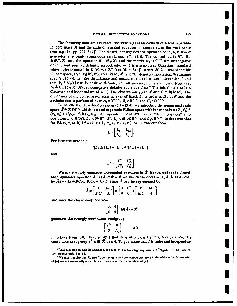
I

OPTIMAL PROJECTION EQUATIONS 129 1The following data are assumed. The state x(t) is an element of a real separable

Hilbert space W and the state differential equation is interpreted in the weak sense(see, e.g., [6, pp. 229, 317]). The closed, densely defined operator A: a (A)c a*-+ Y

generates a strongly continuous semigroup eA', tO. The control u(t)ER', Be90(R', Y) and the operator R e 0(X) and the matrix R2 ER" X- are nonnegative Idefinite and positive definite, respectively. w(.) is a zero-mean Gaussian "standardwhite noise process" in L2((O, 00), Y') (see [6, p. 314]), where N" is a real separableHilbert space, H, e M2(X, X), H2 e _1(W', R') and "E" denotes expectation. We assumethat HH* = 0, i.e., the disturbance and measurement noises are independent,3 and Ithat V2 A H2H* eR' is positive definite, i.e., all measurements are noisy. Note thatV, A HH* I %(Ye) is nonnegative definite and trace class.' The initial state x(O) isGaussian and independent of w(.). The observation y(t)eR' and Ce (k, R'). The Idimension of the compensator state x,(t) is of fixed, finite order n, dim Ye and theoptimization is performed over A, c R - 'x , , Be R "x and C, e R .

To handle the closed-loop system (3.1)-(3.4), we introduce the augmented statespace itA X R', which is a real separable Hilbert space with inner product (i,, i2 )A I(xt,x 2)+xrx12, RiA(xxj). An operator LeSI(W) has a "decomposition" intooperators LIE M(X), L1 2 E 0(R%,, X), L2je 0(YeR") and L2eR ' , '", in the sense that

~Ifor i A(x, x)e U L= (Ljx + L 2x, L21x+ L2x,), or, in "block" form,

For later use note that L 2 LI]I

and 1L 1 -1I,1 + 11 L,211 + 15L + 11 L2211

L* [

We can similarly construct unbounded operators in . Hence, define the closed-loop dynamics operator A: e(A)c a'-- * on the dense domain 9(A)A A (A) XR"',by Ai = (Ax + BCx,, BcCx + Acx,). Since A can be represented by

.4 [ A BC rA 0][o0 BCc1BC AJ=O 0+ BeC AJ

and since the closed-loop operator I

generates the strongly continuous semigroup

it follows from [50, Thim., p. 497] that A is also closed and generates a stronglycontinuous semigroup e ' M (*), t : 0. To guarantee that J is finite and independent I

3This assumption and its analogue, the lack of a cros-weighting term x(t)rR 2u(,) in (3.5), are for

convenience only. See 15.

' We must require that R and V, be nuclear since covariance operators in the white noise rormulationof [6] are not necessarily trace class as they are in the formulation of [4].

II

I

130 D. S. BERNSTEIN AND D. C. HYLAND

of initial conditions we restrict our attention to the set of admissible stabilizingcompensators

sl A{(A, B. C,): e*A' is exponentially stable).

3Hence if (A Bo, C,) E 0 then there exist a > 0 and P > 0 such that

(3.6) Ile '1ra e- 0', 1o.Since the value of J is independent of the internal realization of the compensator, wecan further restrict our attention to

if+ A{(A, Bc, C,)E .4: (A, Bc) is controllable and (C, A,) is observable}.

The following lemma is required for the statement of the Main Theorem.LEMMA 3.1. Suppose 4Q, Pc (W) have finite rank and are nonnegative definite.

Then QP is nonnegative semisimple. Furthermore, if p( QP) = n, then there exist G,3 IrE M(X, R",) and positive-semisimple M e R',x", such that

(3.7) 0^ = G*Mr,

(3.8) 7Gor* =..

Proof. By Lemma 2.4 there exists a finite-dimensional subspace .X( - W such thatQA c ., QA(' = 0, PAN - A and P.R' = 0. Hence there exists an orthonormal basis1 for X with respect to which t and P have the infinite-matrix representations

0I P.= , 1where Q1h P1 a R'- t are nonnegative definite and r-,dim . Since by Lemma 2.6 thereexists invertible T e R" " such that A1 = ' ,I-1 P3'J' is nonnegative diagonal, we have

which shows that 0 P is nonnegative semisimple. If, furthermore, p(Q P) = n, then itis clear that * can be chosen (i.e., modified by an orthogonal matrix) so thatU 0_10 0

3 where A e R'' ", is positive diagonal. Hence,

N =L~; f[['O"]A[[II O. 0] 0~~~ iwhich shows that (3.7) and (3.8) are satisfied with

for all invertible S e R"'- '". 0We shall refer to G, rE R(Y, R", ) and positive-semisimple Me R",'", satisfying

(3.7) and (3.8) as a (G, M, r)-factorization of QP. For convenience in stating the Main

Theorem define

A X BR 2 1B*, LCO V2 C.

II

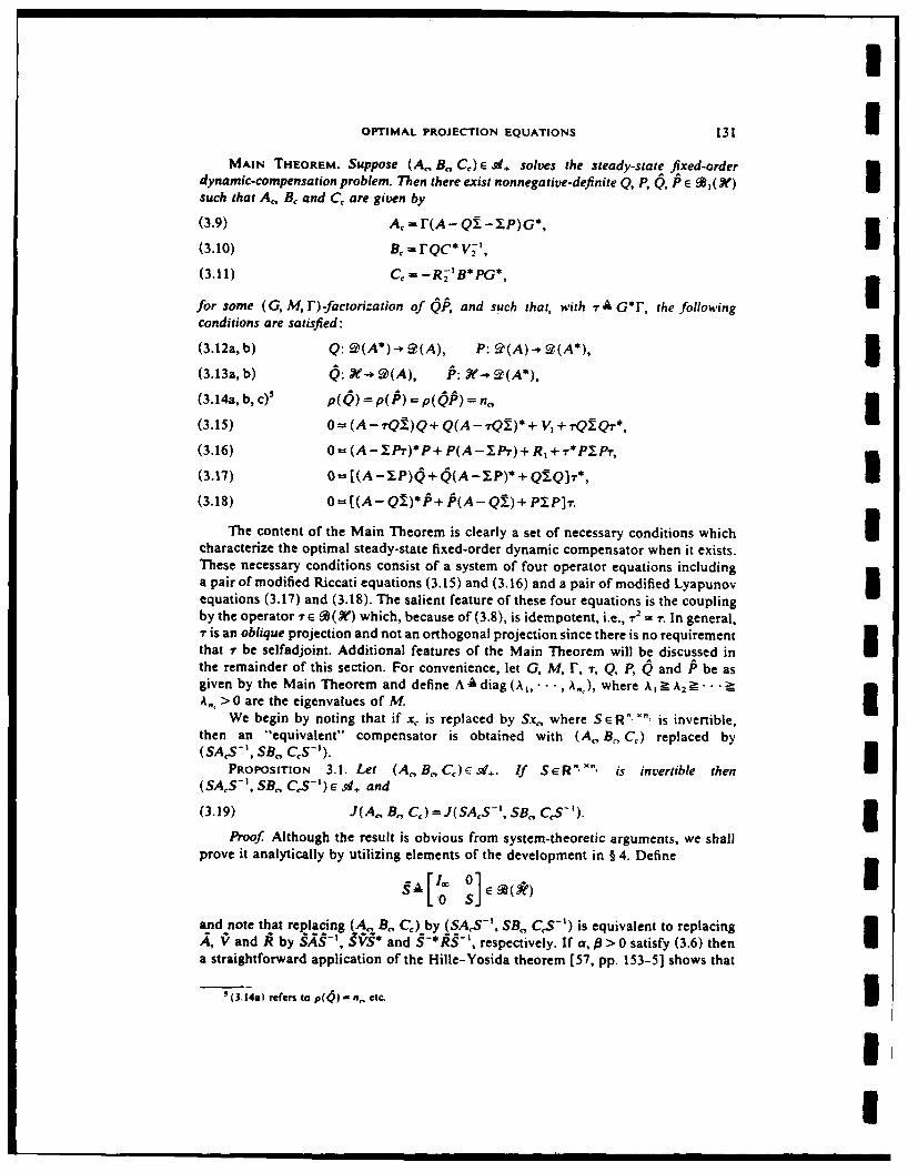
I

OPTIMAL PROJECTION EQUATIONS 131 1MAIN THEOREM. Suppose (A. B,, C,) E 51. solves the steady-state fixed-order

dynamic-compensation problem. Then there exist nonnegative-definite Q, P, , P ( 9a,) such that A Bc and C, are given by

(3.9) Ac = r(A - Q1- 3P)G*,(3.10) Bc = FQC* V2-,(3.11) cc = -R 2- B* PG* ,

for some (G, M, F)-factorization of QP, and such that, with r-A G'F, the following Iconditions are satisfied:

(3.12a, b) Q: _q (A*)-.?(A), P: 2 (A).--t,(A*), 3(3.13a, b) 4 : X- 9(A), i$: X- 2WA),

(3.14a, b, c)' p(6) = p(P) = p(56) = nl

(3.15) 0= (A - rQ.)Q + Q(A - rQY.) * + V, + rQTQ Qr*,

(3.16) 0 = (A -X.Pr)*P + P(A - .Pr) + R, + r* P.P,

(3.17) 0 = [(A -IP) d + 0(A - YP)* + Q:.Q]-*,

(3.18) 0 = [(A - QE)* P + P(A - Q!) + P.. P].

The content of the Main Theorem is clearly a set of necessary conditions which Icharacterize the optimal steady-state fixed-order dynamic compensator when it exists.These necessary conditions consist of a system of four operator equations includinga pair of modified Riccati equations (3.15) and (3.16) and a pair of modified Lyapunov Iequations (3.17) and (3.18). The salient feature of these four equations is the couplingby the operator iE a(K) which, because of (3.8), is idempotent, i.e., r'= ,r. In general,,r is an oblique projection and not an orthogonal projection since there is no requirementthat 7 be selfadjoint. Additional features of the Main Theorem will be discussed in 1the remainder of this section. For convenience, let G, M, 1, 7, Q, P, Q and P be asgiven by the Main Theorem and define A A diag (A,.., A,,), where A-A 2

. .

A,., > 0 are the eigenvalues of M. IWe begin by noting that if x, is replaced by Sx , where SER"," is invertible,

then an "equivalent" compensator is obtained with (A, B, C,) replaced by(SAS - ', SB, C S-).

PROPOSITION 3.1. Let (A. B. C,)E d+. If SeR"'", is invertible then(SAS-, SB. C,.S-) c s+ and

(3.19) J(A, B,, C) = J(SAS-', SB, CS-').

Proof Although the result is obvious from system-theoretic arguments, we shallprove it analytically by utilizing elements of the development in § 4. Define

1"c~ 0 ]E

and note that replacing (A. B , C) by (SAS - ', SB, C-.') is equivalent to replacing,A, V and A by - fV and S-*A-, respectively. If a, # > 0 satisfy (3.6) thena straightforward application of the Hille-Yosida theorem [57, pp. 153-5] shows that

'(3.14s) refers to p(4) -n , etc. I

II

U 132 D. S. BERNSTEIN AND D. C. HYLAND

the strongly continuous semigroup generated by S' S-' satisfies tie$''1_"ii s s' -a e 9 , which proves the first assertion. Since S eA'S -

, 0, is also a stronglycontinuous semigroup with generator S it follows that S • S = e . Hence

I J e -(SS'*) e(')I- ' dt-: SdOt

and (3.19) follows from tr QA = tr ( (*)( -. A-I) 0In view of Proposition 3.1 one would expect the Main Theorem to apply also to

(SACS - ', SB,, C-'). Indeed, it may be noted that no claim was made as to theuniqueness of the (G, M, F)-factorization of QP used to determine A, B, and C in(3.9)-(3.11). These observations are reconciled by the following result which showsthat a transformation of the compensator state basis corresponds to the alternativefactorization QP = (S- G)T (SMS-')(SF) and, moreover, that all (G, M, F)-factoriz-ations of P are related by a nonsingular transformation. Note that -" remains invariantover the class of factorizations.

PROPOSITION 3.2. IfS e R",' is invertible then , A S- r A SF and A - SMS-satisfy

(3.7)'

(3.8)' = I..3 Conversely, if , re a(, R ) and invertible M? r R "'"' satisfy (3.7)' and (3.8)', thenthere exists invertible S Rnm " such that 5 = S-TG, r = Sr and M = SMS-'.

Proof. The first part of the proposition is immediate. The second part follows bytaking SAm- rG*M- 1, noting S-l=MrG*I - ' and using the identitiestG*MFr*=lM and Mr*= I'G*A. 0

The next result shows that there exists a similarity transformation which simul-taneously diagonalizes QP and 7.

PROPOSITION 3.3. There exists invertible 4) E ( ) such that

(3.20a, b) = - ]4*, . = *Ap 0 ,

(3.21 a, b) Q'@' A 00D' r =@-[ 0'0 (',

i where Ad, A6e Rn",X " are positive diagonal and AdAp = A. Consequently,

(3.22a, b) = 4, P = xr-.

Proof Proceeding as in the proof of Lemma 3.1, choose an orthonormal basis forX with respect to which

*= 0] and .6=[P' 0],0 0 [ 0 0 0

where Q,, PIERR" ' are nonnegative definite. By [55, Thin. 6.2.5, p. 123], there existsinvertible teR " ' such that .OA&P(,V and A =-IT-I are nonnegativediagonal. Because of (3.14), it is clear that W can be chosen so that

* A=[A0 0] and X=o A ],I

U

OPTIMAL PROJECTION EQUATIONS 133 1where A0 , Ape R",'"-are positive diagonal. Thus (3.20) holds with 3

From (3.20) it follows that i

0,= -IAA 0]0cZ0

Now define 03 =[1., 010*, R =AoAp and r =[I,. 0]4) so that (3.7)' and (3.8)' aresatisfied. By the second part of Proposition 3.2 there exists invertible Se R", '", suchthat 0 = S T 0, M = S-MS and r = S-r. Since M and R have the same eigenvalues,M = A (modulo an ordering of the diagonal elements) and thus (3.21a) holds. Finally, U(3.21b) follows from

T=G~rG*4 1, 0]4).0

Remark 3.1. Proposition 3.3 shows that A,," • •, A, are the positive eigenvaluesof 'P.

Remark 3.2. The simultaneous diagonalization in (3.20) has been effected by acontragredient transformation [55], [58]. For applications of this type of transformationto model reduction and realization problems see [12], [59]-[61]. Simultaneousdiagonalization of operators is discussed in [53, p. 181]. I

The following result validates the precise handling of the unbounded operator Ain (3.9), (3.17) and (3.18).

PROPOSITION 3.4. The following relations hold: 5(3.23a, b, c) p(G) = p(r) = p(r) =no

(3.24a, b) r: X - S(A), 7* : 4(A*),

(3.25a, b) G*:R"- 2(A), r* :R", -!@(A*).

Proof From (3.8) and (2.1) it follows that nc = p(rG*) g min {p(r), p(G*)}. Sincep(]F) - n_ p(G)=p(G*) and p(G) < n,, (3.23a) and (3.23b) hold. To show (3.23c) Ieither note (3.21b) or use (3.14a) and (3.22) to obtain

nT = p(Q)p(TQ)()p(.")--p(G*r) p(r)= nc. i

To prove (3.24a) note that (3.22a) implies R(4)c a(-r) and thus p( ) = p(r) impliesR(Q) = *(r), and similarly for (3.24b). Finally, (3.25) follows from (3.23), (3.24), thedefinition 7 = G*F and the fact that r* = r* G. 0

Since the domain of A may not be all of X, expressions involving A require specialinterpretation. First note that because of the range condition (3.25a), the expression(3.9) indeed represents an n, x nc matrix (see, e.g., [6, p. 80]). Similarly, because ofTI(3.25b), AC is given by

(3.26) A . G(A* - .Q- )r*.

With regard to (3.15), note that because of (3.12a), the right-hand side of (3.15) is alinear operator with domain 9(A*). Since e A -,rQ. -Q:EQr* + V +,QQr* isicontinuous on W(A*), AQ+ QA* has a continuous extension on X given precisely by-0. Similar remarks apply to (3.16). Analogous domain conditions were obtained in[5] for a deterministic infinite-dimensional linear-quadratic control problem with

II

I

1 134 D. S. BERNSTEIN AND D. C. HYLAND

full-state feedback. Finally, because of (3.24) the right-hand sides of (3.17) and (3.18)denote bounded linear operators on all of o.

It is useful to present an alternative form of the optimal projection equations(3.15)-(3.18). For convenience define the notation

PROPOSITION 3.5. Equations (3.15)-(3.18) are equivalent, respectively, to

(3.27) 0 = AQ+ QA*+ V, - Q!Q+ i Q.Qr*,

(3.28) 0 = A*P+ PA + R, - PIP + r* PYP'r,

(3.29) O=(A-.P) +4 (A-IP)*+Q!Q-%Q1QT'*

(3.30) 0 = (A - Ql).P +P (A - QT)+ P.P - P.Pr,.

Proof The equivalence of (3.27) and (3.28) to (3.15) and (3.16) is immediate.Using (3.22a) in the form Q = Q7*, we obtain (3.17)= (3.29)-r*. Conversely, from(3.22a) and [(A -P)Q]* = Q(A -P)* (see, e.g., [6, p. 80]) it follows that (3.29) =

(3.17)+(3.17)*-T(3.17). Similarly, (3.18) and (3.30) are equivalent. 0The form of the optimal projection equations (3.27)-(3.30) helps demonstrate the

relationship between the Main Theorem and the classical LQG result when dim X = n <oo. In this case we need only note that the (G, M, I)-factorization of 4OIP in the"full-order" case n, = n is given by G = r = I, and M = QPf. Since T = I,, and thusT, = 0, (3.27) and (3.28) reduce to the standard observer and regulator Riccati equationsand (3.9)-(3.11) yield the usual LQG expressions. Furthermore, note that in thefull-order case

(3.31) A =A+BCc-BC

and (3.29) and (3.31) can be written as3 (3.32) 0= (A + B C)Q+ Q(A,+ BcC)T+ BcV 2Bc,

(3.33) 0 = (Ac - BCQ)r/ + P(A,- BCQ)+ CTR 2 C,.

Since, as is well known, the stability of A corresponds to the stability of A + BCcAc + B¢C and A - BcC = A, - BC, it follows from standard results (e.g., [62, pp. 48,277]) that the positive-definiteness conditions (3.14a, b) are equivalent to the assump-tion that (A. B, .C) is controllable and observable.

To obtain a geometric intepretation of the optimal projection we introduce thequasi-full-state estimate

I i(t) A G*x (t)E C-so that Ti(t)= e(t) and x(t)= ri(t). Now, the closed-loop system (3.1)-(3.4) can be

written as

(3.34) *(t) = Ax(t) - BCt1(t)+ H,w(t),

(3.35) x(t) = r(A + BC - BC)Ti(t)+ TBC(Cx(t) + H 2w(t)),3 where (3.35) is interpreted in the sense of (3.34) since i(t) e *T and where

4 4A QC*V', ,A -R2'B*P.

It can thus be seen that the geometric structure of the quasi-full-order compensator isentirely dictated by the projection T. In particular, control inputs r(t) determined by

II

OPTIMAL PROJECTION EQUATIONS 135 U(3.35) are contained in g(7) and sensor inputs "By(t) are annihilated unless they arecontained in [.r(?)]± = ("*). Consequently, 9(.r) and 9(v*) are the control andobservation subspaces, respectively, of the compensator. Since r is not necessarily anorthogonal projection, these (finite-dimensional) subspaces may be different.

From the form of (3.35) it is tempting to suggest that the optimal fixed-order Idynamic compensator can be obtained by projecting the full-order (infinite-dimensional) LQG compensator. However, this is generally impossible for the followingsimple reason. Although the expressions for A,, B, and C, in (3.9)-(3.1) have theform of a projection of the full-order LQG compensator, the operators Q and P in I(3.9)-(3.11) are not the solutions of the usual LQG Riccati equations but instead mustbe obtained by simultaneously solving all four coupled equations (3.15)-(3.18). Thisobservation reinforces the statement made in § 1 that the optimal fixed-order dynamic Ucompensator cannot in general be obtained by LQG followed by closed-loop controllerreduction as in [14] and (15].

We now give an explicit characterization of the optimal projection in terms of 1and P. Since QP has finite rank, its Drazin inverse (Qpi)D exists (see [63, Thin. 6, p.108]) and, since (QP)2= G*M 2r, and hence p(Qp) POP), the "index" of QP (see[63], [64]) is 1. In this case the Drazin inverse is traditionally called the group inverseand is denoted by (IP), (see, e.g., [64, p. 124] or [65]). I

PROPOSITION 3.6. The optimal projection T is given by

(3.36) 7 = I(Q ),.

Proof It is easy to verify that the conditions characterizing the Drazin inverse[63] forthe case that QP has index 1 are satisfied by G*M-F. Hence (66), = QPM-Irand (3.8) implies (3.36). 0

We now give an alternative characterization of the optimal projection by introduc-ing the following notation from [51, p. 73]. For 41, e X define the operator 0® ,E

(X) by 3and note that p(o®@)4)= I if 4, and 41 are both nonzero and (0 ®/v)*=# ®6. Usingthis notation, (3.21a) can be written as I(3.37) Q -= Q P) iG ,

where , is an orthonormal basis for . In terms of the Riesz bases (see e.g., [52,p. 309])

(3.37) is equivalent to

(3.38) Q= A ,4®, Iwhich can be regarded as a specialized spectral decomposition of a semisimple operator.We emphasize that, in contrast to the singular value decomposition for compactnonnormal operators (see, e.g., [50, p. 261]), the A, in (3.38) are eigenvalues of QP(see Remark 3.1), not singular values. Moreover, although {46 }'.1 and {e,] . are basesfor Y, they are not necessarily orthogonal. They are, however, biorthonormal, i.e.,(0i, O'A= 8,, and hence 4,®4V, is a rank-one projection and (40,®,)(6j®@i) =0, i #j.

II

i 136 D. S. BERNSTEIN AND D. C. HYLAND

Since r is a rank.n. projection, it is not surprising that r is given precisely by

(3.39) .

The following result summarizes the above observations.NOPOSrTON 3.7. There exist biorthonormal linearly independent sets {.,}1 .,

19(A) and {,}-c ,(A*) such that (3.38) and (3.39) hold. Furthermore, if the(G, M, r)-factorization of QP is chosen such that M = A, then, for all x E W,

Ox WC(, ,01), • • • ,(X, 00,)),

rx = ((x, 4,),. . (X, 0,,,))T.I I Remark 3.3. Note that and '* are given by

and, for all y A(y" .. Y,,)TERI*, G* and I* satisfy

G*y = MY", r*y = 2 YA.

4. Proof of the Main Theorem. We state and prove a series of lemmas which allowus to compute the Frechet derivatives of J with respect to A, B, and C, Requiringthat these derivatives vanish leads to the necessary conditions in their "primitive"form. A transformation of variables then leads to the form of the necessary conditions(3.9)-(3.18).

Let "u-lim" denote the uniform limit (i.e., limit in operator norm) for boundedlinear operators [50, p. 150] and, for strongly continuous S(t) E() t 0, interpretthe strong integral 1:, S(t) dt according to Q S(t)z dt, z e ge [50, p. 152]. Also recallthe standard fact [6, p. 186] that (eA)* = e ' and similarly for A. Throughout thissection let (A,, B, C,) 6 d, and let a, 0 > 0 satisfy (3.6).

To begin, note that the closed-loop system (3.1)-(3.4) can be written as

(4.1) ;U(t)+ Aw(t),

where

H, E E(eR).L BCHZJ

3 For convenience define the nonnegative-definite operator

0n * BVBj, 0T

I In terms of the augmented state g(t), the performance criterion (3.5) becomes

(4.2) J(A., B., C ) - liraEm t, t)

where the nonnegative-definite operator R is defined by

A , 0[ go

I

I

OPTIMAL PROJECTION EQUATIONS 137 1To write (4.2) in terms of the covariance of i(t), recall [6, p. 308] that the

covariance "E[(f-Ef)( -Ee)*]" of a Hilbert-space-valued weak random variableis defined to be the nonnegative-definite operator S which satisfies

(Sy, z) = E( - Ef, y)(f - Efe, z)1

for all y, z in the Hilbert space. Hence define [6, p. 317]45(t) A E[(:Z(t) - EU(t) )(i?(t) -UE(t))*].

LEMMA 4.1. Q A u-lim,-.r (5(t) exists and is given by(4.3) Q :e/ fle"*' dt.

Furthermore,(4.4) J(A., B,. C,) = tr 45k

Proof. First compute (as in [6, p. 317])

((5(t);, z) E(i(t) - eAiEi(0), y)(i(t) - eA4Ei(O), z)

= E(f eA,-s) iA(s) ds, eAd(o,, .)dr,

+(Q5(0) e Af;, e Arti)

=E E E (i(s), A* eA (t-S)y)(v(cr),t* eA '('-ca)z) dsd.,

+(eA,0(0) e;" , z)

=o (eA(13) f/eA(r5), z-) ds +(e-4'0(0) eAt$, z),

which shows that C(t) is given by

45(t) = eA'4Q(0) ea+f eAVeA ' ds.

Clearly, (4.3) makes sense as a strong integral since

To demonstrate uniform convergence it need only be noted that

- s e()l= sulSp I e0-d-(t)wll

SU le A. ekil ds eA (O) e,-f , IleA' feA "ll as + 11 e4'4(O) e A*,,

g 1a2 fll P -' e- "0'+ 110(0)11 - '. 1

II

I138 D. S. BERNSTEIN AND D. C. HYLAND

Next, let I be an orthonormal basis for *t and us e Parseval's equality to obtain

* Since

MO t ? 0

is nonnegative for each n and is increasing in n for each Iwith limit (~()it)monotone convergence permits expectation-limit interchange. Hence using E i(t)eAlEiE(O) we have

I-0- limi {t A 2 (tA"] i~ eAE(O)t2I-C

which by Corollary 2.1 yields (4.4). 0We shall also require the "dual" of Q5 given by

(4.5) P=f e"'R e~'dt.

1 Since V and A are nonnegative definite it is readily seen that Q5 and A are alsononnegative definite.

LEMMA 4.2. , P E 9,(*t).I Pnoof. It suffices to consider Q only since the situation for P is exactly analogous.Since Q is nonnegative definite, Lemma 2.3 can be used. Letting be anorthonormal basis for *t, we have

tr4 = 0, i-iJ) I' "Oj,0

= lim ( eA4 ; e'f,) Ai

Let f.(t) denote the above integrand. Since P is nonnegative definite, {f, }is amonotonically increasing sequence of nonnegative functions such that f,,(t) -tr eAl ~e-", t 0. Hence, by monotone convergence and Lemma 2.2,

Itrt= tr [e~r feksi d

3f =J ie"'f~e"*'j, dtg~a2j1j f, e: -1' dt < o.0

LEMMA 4.3. With d and PS given by (4.3) and (4.5) it follows that

I(4.6) tr AtrA

OPTIMAL PROJECTION EQUATIONS 139 IProof. For any orthonormal basis {0}= of * we have

tr AtrRQ Afe~Att

I _: I A

Letting f. (t) denote the above integrand it follows that f.(t) - tr eA *', t - 0, and

V .( t~l = E I e *' .6" , -k,)j9 a 211 r11 e - 20( C I . ,1

c h o s e n t o

If {4j = is chosen to be the set of orthonormal eigenvectors of A then Lemma 2.1implies Z]. li,4,, ] - Ril and thus lf.(t)l is bounded on [0, 00) by an integrablefunction. Hence by dominated convergence,

tr 45A = ftr [ A eA'Vee" dtAIV tr[eA"R eA ] dt (o,, eAR eA')dt

And again using dominated convergence, 3-1 d0 = 2: (P10j, fJ eAA eAttki dt) = tr 0. 0

The next result is important in that it allows us to treat 4 and P7 as solutions ofdual algebraic Lyapunov equations. For a similar result involving groups rather thansemigroups see [50, pp. 555-557].

LEMMA 4.4. Q is given by (4.3) if and only if QE (*) satisfies(4.7) 45: 9(A-*) 2 (A-),

(4.8) 0 = A10 + A* + f,

where (4.8) holds in the sense discussed in § 3. Furthermore, P is given by (4.5) if and

only if P e 1 (fe) satisfies

(4.9) P: ().(*,3

(4.10) 0=A*P+PA+ R.

Proof We consider only. To prove necessity let t'> 0. Then for all t E [0, t')and iE g(A*) we can write

e At e A* x = f e (+s f e '+')ids 3Hence, =J e d'fe eA*('1)ida.

(4.11) e- e e'"e = ,AJeAG A*" ( "'" t)A*Rdo -e At,

which shows that e A80 e A-' is strongly differentiable with respect to t for all I e [0, t').In particular, setting t =0 it follows that QeA'"i ie(A) for all ;e 9(A*) (see, e.g.,[6, p. 173] or (50, p. 485]). Performing the differentiation on the left-hand side of

II

1 140 D. S. BERNSTEIN AND D. C. HYLAND

(4.11) and setting t = 0 yields

(4.12) A eA*'i = - f e '" e ' eA* A i'"*da- VeA'"

Now fix ij e9(A*). Then for I t>0, , ,0, we have

,0 eI A " (A), i= 1, 2,A3, • •.,

Now consider the sequence {Ad e * I - , Letting t'= I in (4.12) and using dominatedconvergence to interchange limit and integration (A* is a fixed element of W), itfollows that

(4.13) lrn AO e A e Av VeA *OAida-V;y

Since A is closed, 5i E 9(A). This proves (4.7). Also, since A is closed we have

-nm Ad eA,i = Aj.i,

which with (4.13) implies

and hence ( Ad + 41,4 + fo = 0, ; E !2

as desired.To prove sufficiency let ie 2(A). Then eA"E q(A*), t 0, and hence

d e Asoe Axi= e A(A45+QA*) e At

I Thus

eQso ex tE-di = f e'(Aki+Q4A*) e A*sidS, ieqA*).

Extending k + dA* to all of * we obtain

I *A#4 Afi~ = E eAI~eAsids, i

Letting t-co yields (4.3). 0We now introduce some notation which will prove to be most convenient in the

following results. For (A', B', C')eR"- 'xR" "x R" " define

I and SA A A - & 8,j A Bs - B,, 8c, A C - C,

1 (8.,. 88., Sc) 11II .II0 + 11a, I1 + 08cl.

Furthermore, let A', C" and A' denote ,, V' and A with (Ar B, C,) replaced by

II.

OPTIMAL PROJECTION EQUATIONS 141 U(A', B, C') and define 3 B

6AA ,-A = [68 C 8,A i .'g, V2,5T o ]oh " a~ Bv2 + + aVBC7v+SB,v 2B]'

SA A'-R=I00 CTR2 + +5fR2C++ 5cR 2 ,]" 3We shall also write Q', P' for 5, ,P as given by (4.3) and (4.5) with A V. A replaced

by A', VP', A' and define8f'A0'-, a,A/3,-A3

LEMMA 4.5. i is open.Proof. Let (A,, Bo, C,) e.jd be arbitrary and consider the open set

(4.14) NA {(A B, C:,) e n Rx xR"' xRmxn : l(8A,8a,Bc,)1 <9/2ay},

where ,Amax {1,I~ll, ICII}. Then, since A'=A+8A and SAe 90(K) it follows from ITheorem 2.1, p. 497 of [50], that for all (Ac, B' , C') e N and t ? 0,

11 eA "l 11 Z e(-A+ a' P)# g a e-Pt/2 .

Hence, N- ai, as desired. h0LEMMA 4.6. There exists c > 0 such that

(4.15) 11011 - Cl(,, A 8c), I(4.16) 11411l9 C- 1 05lA., 811, SC,)11,

for all (A', B' , C')e N, where N c d is the open neighborhood of (A,, Bc, Cc) defined 3by (4.14).c

Proof We consider (4.15) only. Since 1IeA"l 9ae-lff2, t 0, (A,, B, C':)e N, itfollows that 3

Ioo .18019E0IeA fl! A- At fl e A* 11 dt !

A,,, Il,1A, ,;9 J(Ile'j 11"h leAf -eAIl + leA Ih 118pll IeA*I + H eA" - e ' Jll hle tjl}di

(4.17) r I(el (Al +ll6l) f e e "A"- ek"l •-'l d3

+ a e-3t2 di + a, H f'l J 0 e(A+IA)t - e~R 1 e-0 2 d," o© (A+&A,)t , -D/2 22

a(211 V'g + 0411) J le el e dr +21

From [50, p. 497], it follows that the perturbed semigroup e(A+ w has an expansion

e(A+0 e e A,+ . U(t), tit0,

II

I

U 142 D. S. BERNSTEIN AND D. C. HYLAND

where U(t) (), t9 0, satisfy the estimatesB LI,(tOfl <- a'+'I6RII' eD111i!.

Hence, for all (A,, B', C') e N,

(4.18) lie (.A+ A) e Atli Y Jj U(t) j ae-p1[e n8A1 11

I From (4.17), (4.18) and the relations 18A11 - Yll(SA., , Sc,)11 < 0/2a and

Jo[ea"Al -1] e 3B'9/2 dt 1(4A,, 8s,,.5c,)I

I it follows that E 3 ,

2a3.#3HII ll- (2U1 VU + il 8dl)ll(8A°. 8.,, bc.)iI

+2 (211B V21I 1188a11 + II V211 I 8a1),

I which yields (4.15). 0 3

Since Q, Pe A(*t) we can writeI , =r[o2 Q,2] r,', ,',]Q 1* Q-,J P, 1P*2 P2J

where Q1 e a(7'), Q1 2e E 9(R',), Q2 e R"-"', and similarly for P1, Pt2 and P2. Notethat Q1, Q2, P, and P2 are nonnegative definite. Also, define the notation

F = 1 [ Z 121

where Z2 1 _2'

Z, A P, Q1 + PI2Q *2, Z12A P, Q12 + P12Q2 ,

Z2 A P 1*2 Q+ P2 Q*2, Z2A P*2Q 1 2 + P2Q2,

and, for (A', B', C') e si, let

I bJ(BA,, as,, 8c)AJ(A,,, B, C')-J(A, B. C,).

LEMMA 4.7. Let (A,, B, C:) e d. Then3 (4.19) 6(8 ,, S , 8 )= .B("'(8 , 8C) + 0(11(8A, h,. 8c)l),

where

(4.20) -(SA, 8D, Sc,) A 2 tr [Z 28A,] + 2 tr [( V2BTP 2+ CZ*)8s,]

+2 tr [+ Q2 T +Z*B).5,

and

(4.21) lim II(B,, 88o, 8c,)l'o(B(A,, 8B,, 8c)11) = 0.

Proof. Combining (4.8) and (4.10) with (4.6), J can be written as

J(A, B. C) = tr (OA + K1f +4 trR[ cl (A' + ) + 1 cl (,4o + OA*)],

IU

OPTIMAL PROJECTION EQUATIONS 143 Iand likewise for (A,, B', C' ), where "cl" denotes closure (i.e., extension) of a boundedoperator to all of . Now using the identity

tr [ 40'A'+ P' 1 ] - tr [ k3R + AV7] = tr [ (,38, + hip ] + tr [ 80kR' 7]

we can compute

8jA(S,, SB, Sc,) =tr [Q3 + P8,] +4 tr [( cl (A*(P+ 8s)+(P + .5).')]+ 2 t r [ 8 s c l ( A ,'* P + J', ') ]*+-, tr [J5 cl (A'('o + 80) + ((5 0,E')

I-' tr[ cl (A*fP+,PA) +P cl (A + )*)I

+ tr [ 6A'+ B's'].

Using A = A + 8 and combining the second, fourth and sixth terms yields I8J(8A,, 8r,, 8c,)= A+fl,

where 3A A tr [SA +P 8)] +1 tr [1(8A +P85R) +P(8A k5 +8)]

= tr [8 +16bo] + 2 tr [8ARP]and I

flA- tr[ cl (A'*8 +58A')+ P cl (A8'0+80'*)I

+ 2 tr [80 cl (A'*P,+ PA') + 8 A cl (k( '+ +"4*) +tr [8,R'+ 6 lP].Hi

Computing

tr A +A8 p] = 2 tr + VBTp 2 8B+2 tr [Q 2 CCR 28c] +tr [P 2 ,8 V 28T, + Q 28TR,s,]i

and

2 tr [5AQ 0 = 2 tr [Z-A, I + 2 tr [CZ* 8B,] +2 tr [Z*BSc,] 3and retaining first-order terms, we obtain (4.20).

To evaluate fl, use (4.8) and (4.10) to replace R' and ia ia the last term in fl andwrite A' = A + BA, to obtain I

il = 2tr[ C cl (A*8 p + pA) +/P cl (A5,) + 6 0 ,)]

(4.22) +4 tr [(i(8,tp + js8A) + P(8BA60 + BO*) ] i

- tr [ c (A'8)+ PA'') + 8 cl (,'Q'+ Q', *)I.

Next we note that

(4.23) trI[1 cl (A*8+ S.pA*)] = tr [8j. cl (AQ+ QA*)].

To see this we observe that by arguments similar to those used in the proof of Lemma4.4 and the fact that 8 s: 2(A)- -(A*) it follows that I

N u -i the = cl (A*Ss+ SpA) e ' dt.Jo H

Now, using the technique of Lemma 4.3 with the role of A played by -cl (,*"B, + 8.,4),

II

I 144 D. S. BERNSTEIN AND 0. C. HYLAND

we see that

Similarly, it can be shown that

(4.24) tr [f cl (A8+ 8OA*)] = tr [BO cl (A*i+ N)].

Now substitute (4.23) and (4.24) into (4.22) and rearrange the second term in (4.22)* so thatst =A Itr [8 0 cl (A*P+ PA) +.8 cl (AQ+ QdA*)]

+1 tr2[,~6P 5)+8(~+()

- tr [8 0 cl (A */,+ PA') + 8p cl (A''+ ('A'*)]

= -4 tr [80 cl (A'*8, + &pA') + Sp cl (A'SO + BOA ) ] .

3 Using (4.8) to obtain0 -A'SO + BOA'* + BAd+ C)t+ S

and (4.10) to obtain a similar relation involving P, we have

A= tr [60(85/P+ P8 A+ )] + tr [Ape + 08 * +)].

Restricting (A,, B', C.) to N (see (4.14)), using Lemma 4.6 and noting that 8 A andSA have finite rank, it follows that there exists c > 0 such that

(4.25) I(tl1 S c, Il(8.., 88",5,)112.

Combining [I with the second-order terms in A yields the desired result. 0LEMMA 4.8. d+ is open.Proof. From the "generic- property of controllability and observability [62, p. 44]

there exists an open neighborhood of (A,, B, C) each of whose elements is minimal.

Combining this fact with Lemma 4.5 yields the desired result. 0LEMMA 4.9. Q2 and P2 are positive definite.Proof First note that expanding the R",'",-component of the Lyapunov equation

(4.8) yields (4.50) below. By a minor extension of results from [66] or [67], (4.50) canbe rewritten as

0= (A,+ BcCQ 12Q27)Q2 + QW(A + BCQ, 2Q2)T+ BV 2Bc ,

where Q+ is the Moore-Penrose or Drazin generalized inverse of Q2. Next note thatsince (A,, Bc) is controllable then so is (A, + BCCQI 2QQ2, B V21

2 ). Now, since Q, andB,,V2BT are nonnegative definite, it follows from [62, Lemma 12.2) that Q2 is positivedefinite. Similar arguments show that P2 is positive definite. 0

Having established Lemmas 4.1-4.9, we can now proceed with the proof of theMain Theorem. Let (Ac, B,, C) e d be as in the Main Theorem and consider (4.19)with (A', B', C') confined to d.. Because .Y: R" " xR ", " xR ' R is a bounded

linear functional and di+ is open, the convergence in (4.21) implies that .Y is preciselythe Frechet derivative of J with respect to (A. B, C). Since +, is open, the optimality

of (A B,, C,) implies

(4.26) 2 (5A, 8,,, ,) = 0

for all (SA,, 81,, SC,). Clearly, (4.26) is equivalent to

(4.27) Z= O,

II

I

OPTIMAL PROJECTION EQUATIONS 145 1(4.28) V2BP TP,+ CZ2, = 0,

(4.29) Q2C "R2 + Z*12B = 0.

Thus, B, and C, are given by

(4.30) B1=-P2jZ 2 1 CV2',

(4.31) Cc= -2B*Z- 2 Q2

Although B, and Cc are now determined in terms of Q and A6 A, remains to befound. Moreover, 4i and P themselves depend (via (4.8) and (4.10)) on Bc and C,Hence our task now is to consolidate and simplify (4.7)-(4.10), (4.27), (4.30) and (4.3 1)to obtain the more tractable conditions (3.9)-(3.18). To this end let us define newvariables I(4.32a, b) QA Q,- Q 2 Q21Q*2, PA P, - PP 'P*,

(4.33a, b) Q, 2 Q2-'Q*2, A P, 2P2'P*.

Clearly, Q and P are nonnegative definite and have finite rank. Since by Lemma 4.2Q, Pe (*), it can be seen that Q1, P, E , (Ye), which implies Q, P E R,(9). To showthat Q and P are nonnegative definite, note that Q is the R(Y)-component of thenonnegative-definite operator 9Q* E 90(f'), where

10[' -, 1 '

Similarly, P is nonnegative definite.From the domain conditions (4.7) and (4.9) it follows that

(4.34a, b) Qj: 9(A*) -. a(A), PI: -(A) - (A*),1(4.35a, b) Q12: R",-- 2(A), P12:R"-.9(A*),

which lead to (3.12) and (3.13).Next note that (4.27) is equivalent to (3.8) with

(4.36a, b) G A Q21Q*, r A -P'1P*2

and that (3.7) holds with

(4.37) M -A Q 2P2.

Since Q2 and P2 are positive definite, Lemma 2.6 implies that M is positive semisimple. 3We can also define r= G*r which, by (3.8) satisfies r 2

7. It is helpful to note theidentities

(4.38a, b) Q = Q 12G = G*Q*2, P = -P12r = -r*P*, 3(4.39a, b) = G*Q 2G, P = r* P 2r,

(4.40a, b) rG = G*, r = 1,

(4.41a, b) 4 = , = A',

(4.42) Of, = -Q, 2 P* 2

From (3.8) and (2.1) it follows that

(4.43a, b) p(G) = p(r) = n.

(4.44a, b) P(Q 2) = P(P 2) = nc. 3

I

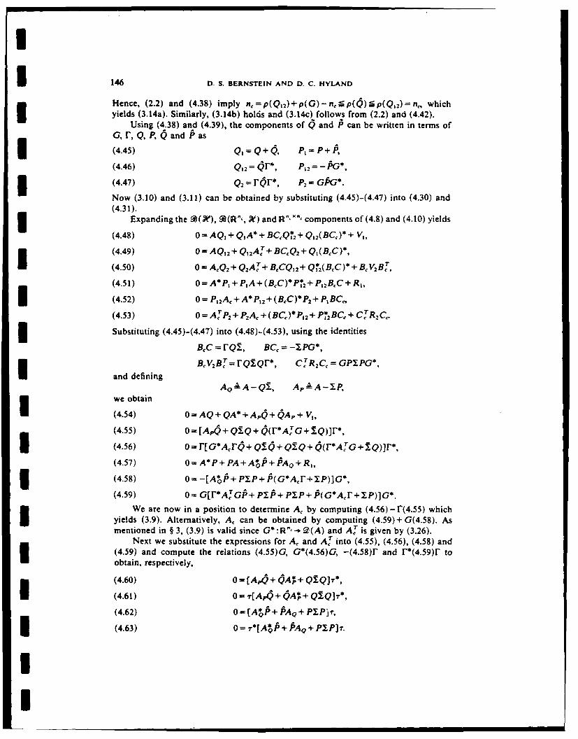
I

I 146 V. S. BERNSTEIN AND D. C. HYLAND

Hence, (2.2) and (4.38) imply n,=p(Q12)+p(G)-n <-p( );-P(Q,2)=ne, whichyields (3.14a). Similarly, (3.14b) holds and (3.14c) follows from (2.2) and (4.42).

Using (4.38) and (4.39), the components of Q and P can be written in terms ofG, r, Q, P, Q and A& as

(4.45) Q,= Q+Q, P=P+P,

(4.46) Q12 = Qr*, P. = G*

(4.47) Q2=r 'r*, P2 = GG*.

Now (3.10) and (3.11) can be obtained by substituting (4.45)-(4.47) into (4.30) and(4.31).

Expanding the 6(ge), R(R",, X) and R", x" components of (4.8) and (4.10) yields

(4.48) 0 = AQ + Q, A* + BCCQ*2+ Q12(BC)* + Vi,

(4.49) 0= AQ 12 + Q12Ar + BCQ 2 + Q,(B C)*,

(4.50) 0 = AcQ 2 + Q2A[ + BcCQ2 + Q*2(BC )* + B V2B ,

(4.51) 0=A*P1 +P1 A+(BcC)*P*2+P,,BcC+R,3 (4.52) 0= P,2Ac+A*P1 2 +(B C)*P2+PIBCC,

(4.53) 0 = AlP2 + P2A + (BCc)* P,2 + P*2BC + C R2C,

Substituting (4.45)-(4.47) into (4.48)-(4.53), using the identities

B C = rQ!, BCc = -I PG*,

and defining BCV2B rQ1Qr*, C R 2 Cc = GPIPG*,

Ao -,A A - Q1., A, .- A - I.P,

we obtain

(4.54) 0 = AQ+ QA*+Ap6+ QAp + V,

(4.55) 0 = [A + QQ + ^(F*AlG +,IQ))r*,1 (4.56) 0 = r[G*AroY + Q0 + QSQ + Q(r*A'G +Q)]r*,

(4.57) 0= A*P+ P+Ao+i + Rl,

(4.58) 0 = -[A*Q P + PIP + P(G*Acr+ iP)](*,

(4.59) 0 = G[r* ATGP + PIP + P P + f'(G*Acr + IP)]G*.

We are now in a position to determine A, by computing (4.56) - r(4.55) whichyields (3.9). Alternatively, Ac can be obtained by computing (4.59)+ G(4.58). Asmentioned in § 3, (3.9) is valid since G*:R", - (A) and ACT is given by (3.26).

Next we substitute the expressions for A, and A." into (4.55), (4.56), (4.58) and(4.59) and compute the relations (4.55)G, G*(4.56)G, -(4.58)r and F*(4.59)W toobtain, respectively,

(4.60) 0= [AA + (A* + Q!Q]'*,

(4.61) 0=7-[A,,Q+4A*+QQ]-r*,

(4.62) 0= [A P+ PAQ+ PIPJ),

(4.63) 0= T*[A~fi+ PAQ+ PIP).

II

OPTIMAL PROJECTION EQUATIONS 147 INote that (4.60)-(4.63) are equivalent to (4.55), (4.56), (4.58) and (4.59) since G andr have full rank. Since ( 4 .6 1) =--(4.60 ) and (4.63)= T*(4.62), (4.61) and (4.63) aresuperfluous and can be omitted. Thus we have derived (3.17) and (3.18).

To obtain (3.15) and (3.16) we need only compute the relations (4.54)+ 7(4.60)-(4.60) - (4.60)* and (4.57) + I"*(4.62) - (4.62) - (4.62)* and use (4.41).

Finally, to show that the preceding development entails no loss of generality in Ithe optimality conditions we now use (3.9)-(3.18) to obtain (4.7)-(4.10) and (4.27)-(4.29). Let A,, B , C., G, 1, 7, Q, P, , be as in the theorem statement and defineQ1, Ql,, Q2, P1. P12, P. by (4.45)-(4.47). Note that (3.12) and (3.13) imply (4.34) and(4.35) and hence (4.7) and (4.9). Using (3.8), (3.10), (3.11) and (3.22) it is easy toverify (4.27)-(4.29). Finally, substitute (4.32), (4.33) and (4.36) into (3.15)-(3.18),reverse the steps taken earlier in the proof and use (3.9)-(3.11) to obtain (4.8) and I(4.10), which completes the Proof. r-

5. Concluding remarks. This paper has considered the problem of quadraticallyoptimal, steady-state, fixed-order dynamic compensation for linear infinite-dimensionalsystems. The Main Theorem presents the stationarity conditions of the optimizationproblem in a highly simplified and rigorous form. The "optimal projection equations"(3.15)-(3.18) (or, equivalently, (3.27)-(3.30)) of the Main Theorem reveal the essential 1structure of the first-order necessary conditions and display the central role played bythe optimal projection 7. The relationship of the Main Theorem to the standardfinite-dimensional steady-state LQG problem can be demonstrated by replacing '" withthe identity matrix and noting that (3.27) and (3.28) reduce immediately to the familiarpair of operator Riccati equations and that (3.29) and (3.30) yield the controllabilityand observability gramians of the controller.

Inasmuch as the Main Theorem is a fundamental generalization of classicalsteady-state LQG theory, a number of issues must be reexamined. Hence, in conclusionwe should like to point out some possible extensions of the Main Theorem along withdirections for further research.

1. Sufficiency theory. Although sufficient conditions for the existence of an optimalcompensator were not investigated in this paper, auxiliary conditions based upon thestructure of (3.15)-(3.18) could perhaps be imposed upon Q, P, Q and P to single outthe global optimum from amongst the local minima. This would be similar to thesituation in LQG theory where, under stabilizability and detectability hypotheses,optimal stabilizing Q and P are identified as the unique nonnegative-definite solutionsof the pair of algebraic Riccati equations. I

2. Stabilizability. Just as in the full-order LQG problem, one would expect anatural relationship between the structure of the optimal solution and stabilizabil-ity/detectability hypotheses. The results of [41], [42] and [68] could serve as a startingpoint in this regard.

3. Numerical algorithms. In practical situations, the distributed parameter systemwould be replaced by a high-order discretized model for which the matrix version(rather than the operator version) of the optimal projection equations could be solvednumerically. A numerical algorithm for solving the matrix version of the optimalprojection equations has been developed in [32] and [34]. The proposed computationalscheme is fundamentally quite different from gradient search algorithms [17], [18],[21], [22], [24], [25], [28], [30] in that it operates through direct solution of the optimalprojection equations by iterative refinement of the optimal projection.

4. Convergence. One of the principal uses for the optimal projection equationswill be to understand the relationship between fixed-order dynamic-compensator

II

148 D. S. BERNSTEIN AND D. C. HYLAND

designs which are optimal with respect to approximate models and the optimalfixed-order dynamic compensator for the distributed parameter system itself. By con-sidering a sequence of nth-order approximate models which converge to the distributedparameter system, conditions would be sought guaranteeing that the sequence offixed-order compensators based on each approximate model approach the optimaldynamic compensator based upon the distributed parameter system (see [38]-[40]).This approach is analogous to the convergence results obtained in [7], [8] with themajor difference being that the optimal projection equations permit the order of thecompensator to remain fixed in accordance with real-world implementation constraintswhereas in [7]-[9] the order of the compensator increases without bound.

5. Unbounded control and observation. An important generalization of the problemconsidered in this paper involves the case in which the input and output operators Band C are unbounded. The mathematical details for this problem are considerablymore complex (see, e.g., [69]).

6. Singular observation noise/singular control weighting. As pointed out in [22],[33], [36] the assumptions of nonsingular control weighting and nonsingular observa-tion noise preclude the use of direct output feedback as in

(5.1) uMt = C'xJ(t)+ D)y(t)

since J is undefined unless

tr [DTR2DKV] = 0(4* R,DV 2 = 0).

Although with due attention to (5.1) direct output feedback can be used in the singularcase, the nature of the problem forebodes all of the difficulties associated with thesingular LQG problem. Note that the deterministic output feedback problem [70],when viewed in this context, is highly singular.

7. Discrete-time system/discrete-time compensator. Digital implementation can bemodelled by a discrete-time compensator with control of a continuous-time systemfacilitated by sampling and reconstruction devices. See [71], [73] for results in thisdirection.

8. Cross weighting/correlated disturbance and observation noise. This extension isstraightforward and entirely analogous to the LQG case (see, e.g., [18, p. 351]).

Acknowledgments. We wish to thank Ardeth P. Grant for excellent and carefultyping of the original manuscript version of this paper. Word processing and revisionsupport was provided by Harris Corporation, GASD.I

REFERENCES

[1] M. J. BALAS, Toward a more practical control theory for distributed parameter systems, in Control andDynamic Systems. C. T. Leondes, ed., Advances in Theory and Applications, 19, Academic Press,New York, 1982.

[2] M. ATHANS, Toward a practical theory of distributed parameter systems, IEEE Trans. Automat. Control.,I AC-15 (1970), pp. 245-247.

[3] S. A. RFIBLE. Acoustoelectric convolver technology for. spread.spectrum communications IEEE Trans.Microwave Theory Tech., MTT-29 (1981), pp. 463-473.

[4) R. F. CURTAIN AND A. J. PRITCHARD, Infinite Dimensional Linear Systems Theor', Springer.Verlag.New York, 1978.

[5] J. S. GI SON. The Riccati integral equations for optimal control problems on Hilbert spaces, this Journal.17 (1979), pp.I537-565.

I

I

OPTIMAL PROJECTION EQUATIONS 149 I[6] A. V. BALAKRISHNAN, Applied Functional Analysis, Springer-Verlag. New York, 1981.[7] J. S. GIBSON, An analysis of optimal modal regulation: convergence and stability, this Journal, 19 I

(1981), pp. 686-707.

(8] -, Linear-quadratic optimal control of hereditar y differential systems: infinite dimensional Riccagiequations and numerical approximations, this Journal, 21 (1983), pp. 95-139.

[8a] H. T. BANKS AND K. KUNISCH, The linear regulator problem for parabolic systems, this Journal. 22(1984), pp. 684-698.

[9] H. T. BANKS, 1. G. ROSEN AND K. ITO, A spline based technique for computing Riccati operators andfeedback controls in regulator problems for delay equations, SIAM J. Sci. Stat. Comput., 5 (1984),pp. 830-855.

[10] M. AoxK , Control of large-scale dynamic systems by aggregation, IEEE Trans. Automat. Control, AC- I(1968), pp. 246-253.

(II D. A. WILSON, Optimum solution of model-reduction problems, Proc. lEE, 117 (1970, pp. 1161-1165.[12] B. C. MOORE, Principal component analysis in linear systems: controllability, observabiliDt, and model

reduction, IEEE Trans. Automat. Control, AC-26 (1981), pp. 17-32. I(13] R. E. SKELTON AND A. YOUSUFF, Component cost analysis of large scale systems, in Control and

Dynamic Systems, C. T. Leondes, ed., Academic Press, New York, 1982.[14] E. A. JONCKHEERE AND L. M. SILVERMAN, A new set of invariants for linear systems-application

tp reduced-order compensator design, IEEE Trans. Automat. Control, AC-28 (1983), pp. 953-964.[15] A. YOUSUFF AND R. E. SKELTON, Controller reduction by component cost analysis, IEEE Trans.

Automat. Control, AC-29 (1984), pp. 520-530.[16] T. L. JOHNSON AND M. ATHANS, On the design of optimal constrained dynamic compensators for

linear constant systems, IEEE Trans. Automat. Control, AC-15 (1970), pp. 658-660.(17] W. S. LEVINE, T. L. JOHNSON AND M. ATHANS, Optimal limited state variable feedback controllers

for linear systems, IEEE Trans. Automat. Control, AC-16 (1971), pp. 785-793.[18] K. KWAKERNAAK AND R. SIVAN, Linear Optimal Control Systems, Wiley-Interscience, New York,

1972. U(19] D. B. ROM AND P. E. SARACHiK, The design of optimal compensators for linear constant systems with

inaccessible states, IEEE Trans. Automat. Control, AC-18 (1973), pp. 509-512.[20] M. SIDAR AND B.-Z. KURTARAN, Optimal low-order controllers for linear stochastic systems, Int. J.

Control, 22 (1975), pp. 377-387. I(21] J. M. MENDEL AND J. FEATHER, On the design of optimal time-invariant compensators for linear

stochastic time-invariant systems, IEEE Trans. Automat. Control, AC-20 (1975), pp. 653-657.(22] S. BASUTHAKUR AND C. H. KNAPP, Optimal constant controllers for stochastic linear systems, IEEE

Trans. Automat. Control, AC-20 (1975), pp. 664-666.(23] R. B. ASHER AND J. C. DURRETT'-, Linear discrete stochastir control with a reduced-order dynamic

compensator, IEEE Trans. Automat. Control, AC-21 (1976), pp. 626-627.[24] W. J. NAEIJE AND 0. H. BOSGRA, The design of dynamic compensators for linear multivariable systems,

1977 IFAC, Fredericton, New Brunswick, Canada, pp. 205-212. I(25] H. R. SIRISENA AND S. S. CHOI. Design of optimal constrained dynamic compensators for non-stationary

linear stochastic systems, Int. J. Contr., 25 (1977), pp. 513-524.[26] P. J. BLANVILLAIN AND T. L. JOHNSON, Specific-optimal control with a dual minimal-order observer-

based compensator, Int. 1. Contr., 28 (1978), pp. 277-294.[27] -, Invariants of optimal minimal-order observer-based compensators. IEEE Trans. Automat.

Control, AC-23 (1978), pp. 473-474.[28] C. J. WENK AND C. H. KNAPP, Parameter optimi:ation in linear systems with arbitrarily constrained

controller structure, IEEE Trans. Automat. Control, AC-25 (19801, pp. 496-500.[29] J. O'REI LLY, Optimal low-order feedback controllers for linear discrete-time systems, in Control and

Dynamic Systems 16. C. T. Leondes, ed., Academic Press, New York, 1980.[30] D. P. LooZE AND N. R. SANDELL, JR., Gradient calculations for linear quadratic fixed control structure

problems, IEEE Trans. Automat. Control, AC-25 (1980), pp. 285-288.[31] D. C. HYLAND, Optimality conditions for fixed-order dynamic compensation of .lexible spacecraft with

uncertain parameters, AIAA 20th Aerospace Sciences MIs., paper 82-0312, Orlando, FL, Jan. 1982.[32] -. , The optimal projection approach tofixed-order compensation: Numerical methods and illustrative

results, AIAA 21st Aerospace Sciences Mtg., paper 83-0303, Reno, NV, Jan. 1983.[33] D.C. HYLAND AND D. S. BERNSTEIN, Explicit optimality conditions forfixedorder dynamic compensa.

tion, Proc. IEEE Conference on Decision and Control, San Antonio, TX, Dec. 1983. pp. 161-165.

[34] D. C. HYLAND, Comparison of various controller-reduction methods: Suboptimal versus optimal proec-tion, Proc. AIAA Dynamics Specialists Conference, Palm Springs, CA, May 1984, pp. 382-389.

II

I

150 D. S. BERNSTEIN AND D. C. HYLAND

[35] D. S. BERNSTEIN AND D. C. HYLAND, The optimal projection equations for fixed-order dynamiccompensation of distributed parameter systems, Proc. A IAA Dynamics Specialists Conference, PalmSprings, CA, May 1984, pp. 396-400.

[36] -, The optimal projection equations for fixed.order dynamic compensation, IEEE Trans. Automat.Control, AC-29 (1984), pp. 1034-1037.

[37] - . The optimal projection approach to model reduction and the relationship between the methods ofWilson and Moore, Proc. IEEE Conference on Decision and Control, Las Vegas, NV, Dec. 1984,

pp. 120-126.(37a] - . The optimal projection equations for model reduction and the relationships among the methods

of Wilson, Skelton and Moore. to appear.[38] T. L. JOHNSON, Optimization of low order compensators for infinite dimensional sstems, Proc. 9th IFIP

Symposium on Optimization Techniques, Warsaw, Poland, September 1979, pp. 394-401.[39] R. K. PEARSON, Optimal fixed-form compensators for large space structures, in ACOSS SIX (Active

Control of Space Structures), RADC-TR-81-289, Final Technical Report, Rome Air DevelopmentCenter, Griffiss AFB, New York, 1981.

[40] - , Optimal velocity feedback control of flexible structures, Ph.D. dissertation, Dept. ElectricalEngineering and Computer Science, Massachusetts Institute of Technology, Cambridge, 1982.

[41] R. F. CURTAIN, Compensators for infinite-dimensional linear systems, J. Franklin Inst., 315 (1983), pp.331-346.

[42] J.M. SCHUMACHER, A direct approach to compensator design for distributed parameter systems, this

Journal, 21 (1983), pp. 823-836.[43] D. L. RUSSELL, Linear stabili:ation of the linear oscillator in Hilbert space, J. Math. Anal. Appl., 25

(1969), pp. 663-675.[44] - , Decay rates for weakly damped systems in Hilbert space obtained with control theoretic methods,

J. Differential Equations, 19 (1975), pp. 344-370.[45 M. J. BALAS, Modal control of certain flexible dynamic systems, this Journal, 16 (1978), pp. 450-462.[46] - , Feedback control offlexible systems, IEEE Trans. Automat. Control, AC-23 (1978), pp. 673-679.(47] J. S. GIBSON, A note on stabilization of infinite dimensional linear oscillators by compact feedback, this

Journal, 18 (1980), pp. 311-316.[48] M. J. BALAS, Trends in large space structure control theory: Fondest hopes, wildest dreams, IEEE Trans.

Automat. Control, AC-24 (1982), pp. 522-535.(49] T. L. JOHNSON, Progress in modelling and control of flexible spacecraft, J. Franklin Inst., 315 (1983),

pp. 495-520.[49a] M. J. BALAS, Feedback control of dissipative hyperbolic distributed parameter systems with finite

dimensional controllers, J. Math. Anal. Appl., 98 (1984). pp. 1-24.(50] T. KATO, Perturbation Theory for Linear Operators, Springer-Verlag, New York, 1966.

[51] J. R. RtNcROSE, Compact Non-Se!f-Adjoint Operators, Van Nostrand Reinhold, London, 1971.[52] I. C. Go .

, ERG AND M. G. KREIN, Introduction to the Theory of Linear Nonselfadjoint Operators,Translations of Mathematical Monographs, Vol. 18, American Mathematical Society, Providence,R 1, 1966.

[52a] M. S. BRODSK II, Triangular and Jordan Representations qf Linear Operators, Translations of Mathe-matical Monographs, Vol. 32, American Mathematical Society, Providence, RI, 1971.

[53] 1. GOHBERG AND S. GOLDBERG, Basic Operator Theor', Birkhauser, Boston, 1981.(54] F. R. GANTMACHER, Thle Theorl, of Matrices, Vol. 1, Chelsea, New York, 1977.

[55] C. R. RAO AND S. K. MITRA, Generalized Inverse of Matrices and Its Applications. John Wiley, NewI York, 1971.

[56] B. NOBLE AND J. W. DANIEL, Applied Linear Algebra, Second edition, Prentice-Hall, EnglewoodCliffs, N J, 1077.

[57] R. F. CURTAIN AND A. J. PRITCHARD, FunctionalAnalysis in Modern Applied Mathematics, AcademicPress, London, 1977.

[58] S. CHAKRABARTI, B. B. BAVTACHARYYA AND M. N. S. SWAMY, On simultaneous diagonalizationof a collection ofhermitian matrices, Matrix and Tensor Quart., 29 (1978), pp. 35-54.

[59] C. T. MULLIS AND R. A. ROBERTS, Synthesis of minimum roundoff noise fixed point digital filters,IEEE Trans. Circ. Syst., CAS-23 (1976), pp. 551-562.

[60] A. J. LAUB, Computation of balancing transformation, Proc. 1980 Joint Automation Control Conference,San Francisco, CA, Aug. 1980.

[61] E. JONCKHEERE, Open-loop and closed loop approximations of linear systems and associated balancedrealizations, 1982 Symposium on Circuits and Systems, Rome, May 1982.

(62] W. M. WONHAM, Linear Multivariable Control: A Geometric Approach, Springer-Verlag, New York,

1974.

II

OPTIMAL PROJECTION EQUATIONS 151I

(63] D. C. LAY, Spectral properties of generalized inverses of linear opera tors, SIAM J. Appi. Math., 29(1975). pp. 103-109.

[64] S. L CAMPBELL AND C. D. MEYER. JR., Generalized Inverses of Linear Transformations, Pitman,ILondon, 1979.

[65] P. ROBERT. On the group-inverse of a linear transformation, J. Math. Anal. AppI., 22 (1968). pp. 658-669.[661 A. ALBERT, Conditions for positive and nonneglative definiteness in terms of pseudo inverse, SIAM J.

AppI. Math., 17 (1969), pp. 434-WO.U[67] E. KREINDLER AND A. JAMESON, Conditions for nonnegativeness of partitioned matrices, IEEE Trans.

Automat. Control, AC-17 (1972), pp. 147-148.[68] C. N. NETT, C. A. JAcoBSON AND M. J. BALAS. Fractional representation theory: Robustness results

with applications to finite dimensional control of a class of linear distributed systems, IEEE ConferenceUon Decision and Control. San Antonio, TX, Dec. 1983.

(69] R. F. CURTAIN, Finite-dimensional compensators for parabolic distributed systems with unboundedcontrol and observation, this Journal, 22 (1984), pp. 255-276.

[70] W. S. LEVINE AND M. ATHANS, On the determination of the optimal constant output feedback gainsIfor linear multavarfiable systems, IEEE Trans. Automat. Control. AC-IS5 (1970), pp. 44-48.

[71] M. J. BALAS, The structure of discrete-time inite-dimensional control of distributed parameter systems,Proc. IEEE International Large Scale Systems Symposium. Virginia Beach, VA. 1982.

[72] M. S. GHAVSI AND J. J. KELLY, Introduction to Distributed-Parameter Networks with Application toIIntegrated Circuits, Holt, Rinehart and Winston, New York, 1968.

(73] D. S. BERNSTEIN, L. D. DAVIS AND D. C. HYLAND, The optimal projection equations for reduced-order,discrete-time modelling, extimation and control, submitted for publication.

II

April 1988I3 Finite-Dimensional Approximation for

Optimal Fixed-Order Compensation of

5 Distributed Parameter Systems

U* by

U Dennis S. Bernstein* I. Gary Rosen**Government Aerospace Systems Division Department of Mathematics

Harris Corporation University of Southern CaliforniaMS 22/4848 Los Angeles, CA 90089

Melbourne, FL 32902

IAbstract

5 In controlling distributed parameter systems it is often desirable to obtain low-order, finite-dimensional controllers in order to minimize real-time computational requirements. Standard ap-proaches to this problem employ model/controller reduction techniques in conjunction with LQGtheory. In this paper we consider the finite-dimensional approximation of the infinite-dimensionalBernstein/Hyland optimal projection theory. Our approach yields fixed-finite-order controllerswhich are optimal with respect to high-order, approximating, finite-dimensional plant models. Weillustrate the technique by computing a sequence of first-order controllers for one-dimensional,single-input/single-output, parabolic (heat/diffusion) and hereditary systems using spline-based,Ritz- Galerkin, finite element approximation. Our numerical studies indicate convergence of thefeedback gains with less than 2% performance degradation over full-order LQG controllers for theparabolic system and 10% degradation for the hereditary system.

* This research supported in part by the Air Force Office of Scientific Research under contractF49620-86-C.0002

** This research supported in part by the Air Force Office of Scientific Research under grantAFOSR-87-0351. Part of this research was carried out while this author was a visiting scientistat the Institute for Computer Applications in Science and Engineering (ICASE) at the NASALangley Research Center in Hampton, VA which is operated under NASA contracts NAS1-17070

i and NAS1-18107.

I

I

1. Introduction

Approximation methods for the optimal control of distributed parameter systems have been

widely studied. In particular, the approach taken in [1-121 involves approximating the original

distributed parameter system by a sequence of finite-dimensional systems and then using finite-

dimensional control-design techniques to obtain a sequence of approximating, sub-optimal control

laws, observers, or compensators. Furthermore, in these treatments it was demonstrated that if

the open-loop system is approximated appropriately, then it is possible to guarantee convergence

of the sequence of sub-optimal controllers, observers, or compensators, respectively, to the optimal

controller, observer, or compensator for the original infinite-dimensional system. In addition, it

can also be shown that when the approximating sub-optimal control laws or estimators are applied

to the original system, near-optimal performance can frequently be obtained. These ideas were

pursued in the context of both open- and closed-loop control, in both continuous and discrete-time, Iand for both full-state-feedback control and LQG (i.e., Kalman-filter-based) state estimation and

compensation.

In practical situations, however, it is often of interest to obtain the simplest (i.e., the lowest

order) controller which provides a given, desired feedback performance. This is usually achieved

in one of two ways. Either the plant approximation order is reduced prior to controller design, or,

alternatively, reduction techniques are applied to a given high-order control law. Unfortunately,

the former approach may result in undesirable spillover effects while the latter may yield low-order

controllers of low authority which perform unacceptably. In fact, with the second approach, this 5may occur even when a suitable controller is known to exist. For example, as is shown in [13],

controller reduction techniques may even destabilize the closed-loop system. 3A third, more direct approach involves fixing the controller order a priori, and then optimizing

a performance criterion over the class of fixed-order controllers. In a finite-dimensional setting, a 3set of necessary conditions in the form of four coupled matrix equations (as a direct extension of

the pair of the separated Riccati equations of LQG theory) which characterize the optimal fixed- 3order compensator was derived in [14]. These four equations are coupled via an oblique projection

(idempotent) matrix. In the full-order case, this projection becomes the identity thus effectively Ieliminating the additional two equations, and the necessary conditions reduce to the standard LQG

Riccati equations. i

1 1l II lllllllll l l II I I I II I

IThe notion that this direct (i.e., fixed-finite-order) approach can be applied to distributed

I parameter systems was first suggested by Johnson in [15] and further developed in [16] and [17].

To realize such an approach, however, would require a suitable generalization of the optimality3 conditions for the finite-dimensional fixed-order theory. This result was subsequently obtained in

[18] where the matrix optimal projection equations obtained in [14] for finite-dimensional systems

were extended to a set of four coupled operator Riccati and Lyapunov equations characterizing

optimal fixed-finite-order controllers for infinite-dimensional systems.

1 In developing numerical schemes to actually compute fixed-finite-order compensators for

infinite-dimensional systems, one might consider an approach wherein LQG reduction procedures

5are applied to a sequence of controllers obtained by using finite-dimensional full-order design tech-

niques in conjunction with high-order finite-dimensional plant approximations. However, such an

approach is unappealing for two reasons. First, since such methods are not predicated on the

minimization of a performance index, prospects for convergence are slim. And, second, controller-

reduction methods have not proven to be reliable in producing stabilizing compensators (see, for

example, [13]).

3 Hence, on the other hand, we develop an abstract approximation framework (and ultimately

computational schemes) which combine the infinite-dimensional optimal projection theory of [18]

with the approximation ideas developed in [9-121 for infinite-dimensional LQG problems. More

precisely, our approach involves constructing a sequence of approximating finite-dimensional sub-

spaces of the original, underlying, infinite-dimensional Hilbert state space along with correspond-

ing sequences of bounded linear operators which approximate the given input, output, and system3 operators. Then, by choosing bases for these approximating subspaces and applying the finite-

dimensional optimal projection theory, a sequence of matrix equations characterizing a sequence

of approximating optimal, fixed-finite-order compensators for the distributed system is obtained.

Finally, numerical techniques for solving the matrix optimal projection equations (for example, the

homotopic continuation algorithm described in [191 and [20]) can be used to compute the sequence

of approximating gains.

I Our primary aim in this paper is to describe the general approach we are proposing, to discuss

its implementation, and to demonstrate its feasibility and practicality. We offer no convergence3 arguments here, but rather reserve them for a more theoretical paper to follow. Instead, we consider

the application of our technique to two examples. One involves the control of a one-dimensional,

!2I

II

single-input, single-output parabolic (heat/diffusion) system while the other involves a single-input

single-output one-dimensional hereditary control system. These relatively simple examples have

been used throughout the distributed parameter control literature to illustrate the application of

new theories and techniques. A detailed discussion of the application of our ideas to more complex Icontrol systems, for instance, the vibration control of flexible structures, will also appear elsewhere.

We use spline- based Ritz-Galerkin finite element schemes to approximate the open-loop systems

(one for which convergence can be demonstrated in the LQG case) and present and discuss some

of the numerical results which we have obtained using our general approximation framework.

We now outline the remainder of the paper. In Section 2 we briefly review the infinite-

dimensional optimal projection theory from [18], describe the approximation framework, and derive

the corresponding equivalent matrix equations and feedback gains which characterize the approx-

imating fixed-finite-order compensator. In Section 3 we consider the examples, construct the ap-

proximation schemes, and discuss our numerical findings. Section 4 contains a summary and some

concluding remarks. 52. Optimal Projection Theory and Finite-Dimensional Approximation 3

We consider the following fixed-finite-order dynamic-compensation problem. Given the infinite-

dimensional control system

:(t) = Ax(t) + Bu(t) + Hlw(t) (2.1)

with measurements Iy(t) = Cx(t) + H2 W(t), (2.2)

where t C (0, oo), design a finite-dimensional, nth-order dynamic compensator

:i()= A~x,(t) + B,(t), (2.3)5

u(t) = CXz,(t) (2.4) I

which minimizes the steady-state performance criterion

J(AC,BC,C) -_ lim IE[(Riz(t),x(t)) + u(t)TR 2u(t)]. (2.5) 1t-.coo

For convenience we denote the infinite-dimensional plant by H7; that is, 3rr -A (A,B, C, RI,R 2 , VI,V2 ).3

3 a

I

Here =(t) lies in a real, separable Hilbert space X with inner product (., .),A : Dom (A) c X --+ X is

a closed, densely defined operator which generates a Co semigroup {T(t) : t 'e 0} of bounded linear

operators on X,B E £(IRm , X), and C E Z(X,IR). We assume that the state and measurement

are corrupted by a white noise signal w(t) in a real, separable Hilbert space t (see [21] or [22]),

that H, E Z(t, X), H2 = C(, IR), R, E C(X) is (self-adjoint) nonnegative definite, and that R2

is an m x m (symmetric) positive-definite matrix. We define V = HHI and V2 = H2 Hn, where

( )* denotes adjoint, and assume for convenience that HH = 0 and that V2 is positive definite.

The compensator is assumed to be of fixed, finite order n. (i.e., x.(t) E IR"') and that A0, B0,

and C,, are matrices of appropriate dimension. For further details and discussion on the problem

statement and the above assumptions, see [18].

We summarize here the primary result from [18] characterizing optimal fixed-finite-order con-

trollers. For convenience define Z -A BRO-B and 2 -- C*Vi-C. Also let In. and Ix denote

respectively the n. x n, identity matrix and the identity operator on X.

Theorem 2.1. Let n, be given and suppose there exists a controllable and observable nth-

order dynamic compensator (A0 , B., C.) which minimizes J given by (2.5) and for which the closed-

3 loop semigroup generated by

I- B.C A. c

is uniformly exponentially stable. Then there exist nonnegative-definite operators Q, P, Q, P on X

such that A,, B,, and C. are given by

A. = r(A - Q2 - ZP)G° , (2.6)

B. = rQC'v 1 , (2.7)

C,. = -R,-*B*PG", (2.8)

where Q : Dom(A*) -- Dom(A),P : Dom(A)*-. Dom(A*),Q : X -- Dom(A),P: X -*I Dom(A*), and G, r E Z(X,R ), and such that the following conditions are satisfied:

I rank = rank = rank P = nh, (2.9)

3 c=GMr, rG"= I,., (2.10)

for some M E IR"" Xn.

I

II

o = AQ + QA" + V1 - QZQ + rQfQr, (2.11)

0 = A*P + PA + R1 - PEP + rIPEPr±, (2.12) 30 = (A - EP)40 + O(A - £P)* + QZQ - r.Q2Qr., (2.13)

0 = (A - Q?)*P + P(A - Q2) + PEP - rj.PEPr±, (2.14)

where 3r&0 'F, T.L= IX- r.

It is shown in 1181 that the factorization (2.10) for the nonnegative-definite operators ( and P

satisfying rank 0]P = n. always exists and is unique except for a change of basis in IR'°.It is also

shown in [181 that *: IR:W -* Dom (A*) so that the expression (2.6) is well defined. IEquations (2.11)-(2.14) are, in general, infinite-dimensional operator equations. To actually use

them to compute the optimal fixed-order compensator, a finite-dimensional plant approximation is

required. For each N = 1,2,..., let X' denote a finite-dimensional subspace of X and let pN :X __ ZN denote the corresponding orthogonal projection of X onto rZN. Let AN E £(ZN), BN E

(IR-, XN),CN E C(XN,IRL), RN E Z (ZN), and VIN E £(ZN). We consider the system (2.6)-

(2.14) with the plant IT replaced by the plant ITiN given by

,a N A {AN, BN' CNRN, R2,V'N,V}. ITypically, the operators BN, CN, RN and VN are chosen as BN - PNB, CN = CP N,1RN =pNR1

and V N = PNV1 with the requirement that pN converge strongly to the identity Ix as N -- oo.

The operator AN is chosen so that it and its adjoint satisfy the hypotheses of the Trotter-Kato

semigroup approximation theorem (i.e., stability and consistency, see, for example, [231). That is,

A N is chosen so that limN--,o. TN(t)PNO4 = T(t)#, and limjv..,. TN(t)pNo = T(t)*O, uniformly

in t for t in bounded intervals, for each 0 E X, where TN(t) = exp(tAN), t > 0. We shall say more

about these choices for AN , BNCN, RN , and VIN when we address convergence questions below.

Although with the plant/fN equations (2.11)-(2.14) are finite dimensional, they are still oper-

ator equations. It is their matriz equivalents which are used in computations. Unless orthonormal

bases are chosen for the subspaces XN (which is typically not the case in practice) some care must

be taken to obtain the appropriate matrix system.

5

I

For each N ,2,- let.., let - be a basis for XN and choose the standard bases for all

I Euclidean spaces. For a linear operator L with domain and range ZN or any Euclidean space,

let [LI denote its matrix representation with respect to the bases chosen above. Also, let 4N

3 denote the kNsquare Gram matrix corresponding to the basis (- Ji~v, that is, 0N = (aN, ON),

i,j = 1,2,...,kN. Noting that

[(ANY)] = (ON)-IAN]TON, [(BN)*] -[BN]TON, [(CN)] = (ON)-I[CN]T,

y[(N)] = (ON)-1[j]TN , [EN] = [BNIR l[B N]TN, (2NI = ( N)-I[CN]TVi-[CN],

I Ithe matrix equivalents of the operator equations (2.11)-(2.14) become

S0 - [ANf][Q'N] + [QN](ON)-[AN]TON + [VIN] - [QN[2-N][QN]

+ [rf][qN [2N][q B. ] - (ON) [r I N , (2.15)

0- (ON)- [AN] T ON[PN] + [pN] _ [AN] + [Rf] - [PN I[,B][PN]

+ (ON)-[r{1 T ![PN - [EN ][pN][1{], (2.16)

0 0 - ([AN] - [zN[pN])[QN] + [ BN]( )- ([AN1I- [BI[PB.)TON+ [QN][NIN][QN] - [1-N][ -N1[[ [](0)1 _ [rN , (2.17)

( J.)-(IANI- QNI[NI)T N[pN] + [IB.I([A N]- [QN][ZNI)

I + [PNIM[N][PN] - (,pN)-I[rL]TON[PN][ENr][lPN l.[r. (2.18)

Therefore, if we define the kN x kN nonnegative-definite matrices5 N [QN]( N)-l, poN A ON([pN],

04W [N](ON)-1 PON= N[PBNI,

VNA [VN]() - 1, o N [RN],

EN [BBIR l[BN] T, 2o = [CN]TVi-1[CN],

5 we can solve the matrix optimal projection equations given in [14] corresponding to the matrix

plant model3 4- {[AN]'[BNI],[CN1]'R°BJR 2,voNV 2 }

to obtain the matrices Q1, ', N QN and P0 . The approximating optimal nth-order dynamic

A rN ([A N] - Q0NDON - Z0 ePO)(G )T ,

UB =~ rNQN[CN]?Vi-l,

I =- [ 1pN(NT

6

I

where rON, GN E lRn.xkN," and MN rE IRneX no SaisfyI

0 G rMNJ rN(GNyr In.

wher N NP×W M N MF ~ ~ Go 0o 0 R" ,ad I. .aif

[rN = (G')rroN, [rI N = N - [,N]. 3When an infinite-dimensional controller will suffice, C, = -RjB*P E Z (X, IR ' ) and B, = 5

QC*V 2i E C(Rt, X) are the usual infinite-dimensional LQG controller and observer gains (see [9]).

The operators PQ E C(X) are the nonnegative-definite solutions to the two decoupled operator

algebraic Riccati equations (2.11) and (2.12) with r and r±j formally set to IX and 0, respectively.

Since C. has range in IR' and B, has domain IR', there exist vectors c, = (cl,... ,C) T x- X I

and b = (bX.. . ,&) E =,X such that

[C.X], = (ct, x), i = 1,2,...,,m, x E X, I

and

i= 1 =

The vectors c, and b, are referred to as the optimal LQG controller and observer functional gains

respectively. 3With regard to approximation for the full-order LQG problem, for each N = 1,2,... we take

n, = kN. Then it is not difficult to show that 3CNtPNXz = (c, z), xEX, X

and

B -= (bN)'y, y E IR',N bXN aegiven by CN =C V(4N)-1,ON b N (N)TON

where c 1 E X=XN and bN E X iN are = (B

respectively with E X ZN. The vectors c and bN are referred to as the1

approximating optimal LQG controller and observer functional gains. To compute them we need

only solve two standard decoupled matrix algebraic Riccati equations for the IN x kN nonnegative- Idefinite matrices Q N and PO.

A rather complete convergence theory for LQG approximation can be found in [9J. Essentially,

it is shown there that if the approximating subspaces ZN are chosen so that the projections P N

7

• , , n • nI I I

II

converge strongly to the identity as N -- oo, the operators AN, BN, CN, RN , and V N are chosen

as was described above, and the operators QN and pN are uniformly bounded in N, then QN andpN converge weakly to Q .and P, respectively as N -- oo. This in turn implies that C N

-_ C,

I strongly, B N --+ B., weakly, c' --. cc and bN -- bc, weakly, and the closed-loop senigroup

for the approximating optimal LQG compensator converges weakly to the closed-loop semigroup

for the optimal infinite-dimensional LQG compensator, as N --, oo. If, in addition, the operators

SN(t) = TN(t)+BNCNJ and SN(t) = TN(t) - BNCN are uniformly exponentially stable, uniformly

in N, then QN --+ Q and pN - P, strongly, C N - Cc and B N -- Bc, in norm, CN - cc and

b- bc, strongly, and the closed-loop semigroups converge strongly, as N - oo. If R1' and VN

are coercive, uniformly in N, then SN(t) and sN(t) will be uniformly exponentially stable. If it is

also true that R, and V, are trace class and RJPN -- R and V1 NPN -* V, in trace norm then Q

I and P are trace class and QNpN . Q and pNpN .. p in trace norm as N --+ oo.

Returning to the fixed-finite-order case, we note that in general the approximating optimal

projection equations may not possess a unique solution. However, in [19] it is shown for the finite-

dimens' nal case that it is possible to obtain an upper bound for the number of stabilizing solutions.

I Using topological degree theory, the following result was obtained in [191.

Theorem 2.2. Consider the equations (2.11)-(2.14) with the infinite-dimensional plant IT re-3 placed by the finite-dimensional plant IyN . Let n, denote the dimension of the unstable subspace of

AN and assume that n. > n,. Then in the class of nonnegative-definite operators QN, pN, N, 15N

on X N satisfying rank qN = rank PN - rank NPN nc, there exist at most

(mi n, -- n u n,<rnin(k ,

1, otherwise,

solutions of (2.11)-(2.14), each of which is stabilizing. If, in addition, the plant (AN, BNCN)

is stabilizable by an ncb-order -,ntroller, then there exists at least one stabilizing solution of

U (2.9)-(2.14).

Theorem 2.2 shows that while there may exist multiple solutions to the finite-dimensional op-

5 timal projection equations, in practice this number can be quite small. For example, if nc > n,

and the system is either single input (n = 1) or single output (i = 1) then there exists at most

one solution to (2.9)-(2.14) for the plant 17N . The existence of at least one stabilizing solu-

tion of course depends upon whet , or not the plant is stabilizable by an ncth-order controller

II

I(for relevant results, see [24]). Finally, while it may be possible to stabilize a plant with n. <ne,

this case lies outside the scope of the analysis given in 1191. 33. Examples and Numerical Results 3

We first consider the one-dimensional, single-input/ single-output, parabolic (heat/diffusion)

control system with Dirichlet boundary conditions given by 5ta7 (t, 17) a 2 v (-- a. -j.(t,/) + b(t)u(t) +h()w(t,v,), 0 < ii < 1, t > 0, (3.1)

V(t,0) = 0, V(t, 1) = 0, t >0, (3.2)

Yt = 101 c(i)v(t, ti)d7 + hzw 2 (t), t > 0, (3.3)

where a > 0, and b(.) and c(-) are given by 3b( 7) -= ' # ' 02- -, i l < 17 : 2

0, elsewhere,

andc(')=JT2_1, 71<_ 7=,3C = 1 0, elsewhere,

with 0 < 61 < 62 _ 1 and 0 < yj < 12 : 1. In (3.1) and (3.3), h(.) E L. (0,1),w,(t,') CI

L2 (0, 1),a.a. t E [0,oo), (see [22], p. 314), h 2 is a nonzero constant and w2 (-) is unit-intensity white

noise. 3To rewrite (3.1)-(3.3) in the form (2.1), (2.2), in the usual way we take X = L2 (0, 1) endowed

with the standard L2 inner product, let x(t) = v(t,.),t _ 0, define A : Dom(A) c X --* X by 3AO = aD24 for 0 E DomA -A H2(0, 1) n H0(0, 1), and define B E C(IR, X) and C EC(X,,IR1 ) by

Bu = b(.)u for u E IR1 , and CO = f0 c(vi)4,(i)dj7 , for 4, E L 2 (q, 1), respectively. Furthermore, let j± L 2 (0,1) X IR, set w(t) (wi(t,.),w 2 (t)) E t, and define.H E C(±,.) and H2 E C(X,IR')

by Hz = hi(.)zi and H2 z = h2 Z2 for z = (z,z2) E . I

It is well known (see, for example, [23]) that A is closed, densely defined, and negative definite.

Furthermore, A is the infinitesimal generator of a uniformly exponentially stable, analytic (abstract 5parabolic) semigroup {T(t): t 2 0} of bounded, self-adjoint linear operators on X.

We consider linear spline-based Ritz-Galerkin approximation for the open-loop system. For Ueach N - 2,3,..., let (N-' be the linear spline ("hat") functions defined on the interval [0,11

9

I

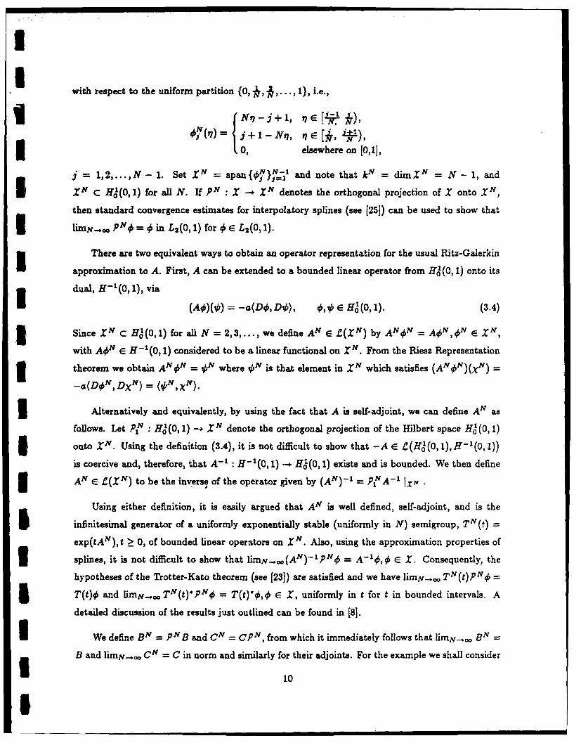
with respect to the uniform partition {0,., ,..., 1}, i.e.,

0,N(M NrI--JNl, q -,E ' t- ),10 0, elsewhere on [0,11,

y = 1,2,...,N - 1. Set XN = span{O4'v}) I and note that kN dimXN = N - 1, and

Z N C Hl(0, 1) for all N. If pN : X _ XN denotes the orthogonal projection of X onto XN,

then standard convergence estimates for interpolatory splines (see [25]) can be used to show that

3 fiMN. . pN 4 = in L2 (0, 1) for 4 E L2 (0, 1).

There are two equivalent ways to obtain an operator representation for the usual Ritz-Galerkin

approximation to A. First, A can be extended to a bounded linear operator from H01(0, 1) onto itsm dual, H-x(0,1), via

(A-0)(0) = -a(DO,DO), 0, E Ho(0,1). (3.4)

3 Since XN C HJo(0,1) for all N = 2,3,..., we define AN E (XN) by AN ON - AON, ON E ZN,

with A46N E H-1(0, 1) considered to be a linear functional on ZN. From the Riesz Representation

3 theorem we obtain AN ON - ON where ON is that element in X which satisfies (AN 'N)(xN)

-a(D4'N, DXN) = (ON,XN ).

3 Alternatively and equivalently, by using the fact that A is self-adjoint, we can define AN as

follows. Let P N : Hol(0, 1) --* XN denote the orthogonal projection of the Hilbert space H0l(0, 1)

onto XN. Using the definition (3.4), it is not difficult to show that -A E Z(H01(0, 1), H- 1 (0, 1))

is coercive and, therefore, that A - ' : H-'(0, 1) -* Ho(0, 1) exists and is bounded. We then define

AN E C(XN) to be the inverse of the operator given by (AN) - I - pNA I N .

Using either definition, it is easily argued that AN is well defined, self-adjoint, and is the

infinitesimal generator of a uniformly exponentially stable (uniformly in N) semigroup, TN ) =

exp(tAN), t >_ 0, of bounded linear operators on XN. Also, using the approximation properties of

3 splines, it is not difficult to show that limjv...(AN)-IPN, = A-',O E X. Consequently, the

hypotheses of the Trotter-Kato theorem (see [23]) are satisfied and we have limN-. TN(t)pN# =5 T(t)O and limN... TN (t)yPN4 = T(t)*',O E X, uniformly in t for t in bounded intervals. A

detailed discussion of the results just outlined can be found in [8].

I We define BN = pNB and CN = CPN, from which it immediately follows that imN--o BN

B and limN.. CN = C in norm and similarly for their adjoints. For the example we shall consider

10I

Ihere, we have chosen R, - riIt,R 2 = r2I,, with rl,r 2 > 0. Setting h1 (q) = vl*,O < q < 1, and

h2 = v2* With v1 ,v 2 > 0, we obtain V, = v Ir and V2 = v2 . We then take RN = pNRI and

VIN- P NVI. For the LQG problem, the open-loop uniform exponential stability of both the

infinite-dimensional system and the approximating systems is sufficient to conclude the strong

convergence of the approximating Riccati operators to the solutions of the infinite-dimensional

Riccati equations, the uniform norm convergence of the approximating controller and observer

gains, and the strong convergence of the functional gains, as N --. co.

Since the basis elements _il are piecewise linear with respect to the uniform mesh

{0, -L, , .. , 1} on [0,1], the equivalent matrix representations for the operators defined above can

be computed directly and in closed form. The Gram matrix = (qNN),i,j=1,2,...,N-I Iis given by O "=- Tridiag{ , , .j}, and if we define the generalized stiffness matrix IPN by

!pm -a(D-',DO'Y),i,j = 1,2,...,N - 1, then ifN = aN Tridiag{1,-2,1}. It follows that 3[AN] = (,ON)-lN,[BN]- ( N)-CbN,[CN] = cN, with b -= (b, ON ) = 0 f2 N(q)dr, and

N = rd(N N N)-1.Ici= (c, q$4) =..-,_ f72 ON(q)di7,i = 1,2,. .. ,N- 1, and that RO 1/ and V =tl¢) 1

For our numerical study we set a = 1, l1 = .75- .03V/2, ,2 = 75 + .04/2, 71 = .25 - .04v2, r2 =

.25 + .03V2,r, = v, = 1,r2 = V2 = 10-4,,h(q) - 1, and used our technique to compute approxi- -mating optimal LQG (i.e., n. = N - 1) and 1st order (i.e., n, = 1) compensators for various values

of N. The open-loop stability of system (3.1)-(3.3) and the approximating systems imply that the

finite-dimensional approximating optimal projection equations have a solution. Theorem 2.2 on the

other hand, with n, = 0 and n, = 1 or n, = N - 1, implies that they have at most one solution.

Consequently, the system of equations (2.11)-(2.14) with the plants H' admits a unique solution.

The optimal projection equations (2.11)-(2.14) were solved using the homotopic continuation 3algorithm described in [19]. It is shown in [19] that the operation count for the algorithm isproportional to p(2n5 + (m + t)n' + (m + 3)ns ) where p is the number of integration steps and n

is the dimension of the finite-dimensional plant. This is competitive with the operation count for

the Hamiltonian solution of the standard Riccati equations which is O(16n3 ) for LQG. Also, note 3that the computational burden for the solution of the optimal projection equations decreases withneC. I

Since m = t = 1 in the LQG case, the optimal functional observer and feedback control gains

b. and c, and the approximating gains b' and cN, are all simply L2 functions with bN and cN 3elements in X N . We plot the functions bN and we obtained for various values of N respectively

11 1• • . .m I I I

IU

in Figures 3.1 and 3.2 below. That convergence is indeed achieved can immediately be observed in

the figures. a..

Ilo t10.0

I 7

0 U-

I U. I oa us . 05Lo .l** .

nBAK CUI4UINATE

Figure 3.1

.4I8

| ..

II I.IO'. I,

, i O ? s I 0- ,.

a. &. . . A . . . 0.7 0.6 0.9 i.4

3 BAR COUJIILNATL

Figure 3.2

12

I

II

In the fixed-order case with n. = 1, the compensator gains A., Bc, and C are all scalars. Also,

for a first-order controller there are only two independent parameters, A, and BQC0. In Table 3.1

below we give the values we obtained for AN and. B9CN for various values of N. Once again,

it is clear that the gains are converging as N increases. In addition, in Table 3.1 we provide the

closed-loop costs JNfQQ and J4' for the LQG and first-order controllers. These closed-loop costs

were evaluated using a 64th-order modal approximation to the infinite-dimensional system. For all 3values of N the performance of the fixed-order compensator was within 2% of the corresponding

LQG controller. Thus, for example, the replacement of a 32nd-order approximating optimal LQG I

controller by an approximating optimal first-order controller will yield considerable implementation

simplification with only minor performance degradation. Note that for the example we consider

here, it is possible to compute the open-loop cost for the infinite-dimensional system in closed form.

We have JoL, =tr fo V 1T'(t)R1 T(t)dt virltr foT(t)2 dt

- rl j e i.dt = ? I2n1011

=12l = 1 .08333.12a 12

Finally, for comparison purposes, we tried applying balancing techniques to the LQG controllers

to reduce their order. However, with n, = 1, such controllers were found to be destabilizing. Based 3upon the results in [13], this was not unexpected. I

N AN BcN JNG 3 I

4 -687.6 5470 .06999 .07014

8 -720.9 5231 .06870 .06993

12 -730.9 5182 .06872 .06991

16 -734.3 5145 .06874 .06990

20 -738.0 5127 .06875 .06990

24 -737.6 5108 .06876 .06990

28 -739.8 5109 .06876 .06990 132 -738.7 5099 .06877 .06990

Table 3.1

113 I

II

As a second example we consider the one-dimensional, single-input, single-output hereditary

f control system given by

i(t) = ao(t) + alv(t - p) + bou(t) + hlw(t), t> O, (3.5)

y(t) = cov(t) + hW(t), t > 0, (3.6)

I where ao, al,bo,co,hih 2 ,p E IR' with h2 6 0, and w is a unit-intensity white noise process. To

rewrite (3.5), (3.6) in the form (2.1), (2.2), we take X = IR1 x L2 (-p,O) endowed with the usual

5 product space inner product, ((7, 0), (C, 0)) = -C fo . , and let z(t) = (v(t), vt), t > 0, where

for t 0, ut E L 2(-p,0) is given by vt(8) = v(t+e), -p < 0 < 0. Define A: Dom(A) C X --+ X by

I A# = (ao40(0) + a1I (-p),D ) for $ = (0(0),0) E Dom(A) _ {(, 0) E X: 0 E H'(-p,0), (0) =

C}, and let B E C(JR,X) and C E C(X,IR') be given by Bu = (bou,O) and C(27,0) =c0,3 respectively. Let t = IR1 and define HI E Z(t,Z) and H2 E .C(t,JR') by Hiz = (hiz,0) and

H2z = h2 z, for z E IR 1 .

3 The operator A is densely defined and is the infinitesimal generator of a Co senigroup {T(t): t

0} of bounded linear operators on X with T(t)(q,) = (v(t; r, ), v (17, .)), t ! 0, where i(-; 7 , )3 is the unique solution to (3.5) with bo = h= 0, and initial conditions v(O) = l,= . We take

R, E C(X) and R 2 E C(IR) to be Ri(q, ) = (riq,0) and R 2u = r2 u, respectively, with r1 ,r 2 > 0.

The definitions of HI and H2 given above imply that V, E C(X) and V2 E C(IR') are given by

Vi(t, ) = (h2 , ,0) and Vz = h z, for (q,4) E X andz IR1 .

I We employ an approximation scheme recently proposed by Ito and Kappel in [26]. We briefly

outline it here; a more detailed discussion can be found in [26]. For each N = 1,2,... let X E

L2(-p, 0) denote the characteristic function for the interval [-jp/N, -(j - 1)p/N),.j = 1, 2,. .. , N,

and let ZN be the (N + 1)-dimensional subspace of X defined by

I ZN span{(1,), (0,XN),..., (0,XN)}.

3 Let PN: X --+ X" denote the orthogonal projection of X onto ZN. Let { _} =o denote the linear B-

spline functions defined on the interval [-p, 0] with respect to the uniform mesh [-p,..., -p/N, 0),and set Z = span {( (0), g)}I= 0. Then X' is an (N + 1)-dimensional subspace of Dom(A)

and it is not difficult to demonstrate that the restriction of pN to Z is a bijection onto XZN. Using

the fact that A restricted to ZN has range in XN, we define AN E C(XN) by AN = A(pN) - ,

and set TN(t) - exp(ANt), t _ 0. Noting that R(B) C ZN, we take BN E Z(IR', ZN) to be giveng by BN = B. Similarly, we take RN = R, and V1 'N = V1. We set CN = C.

14I

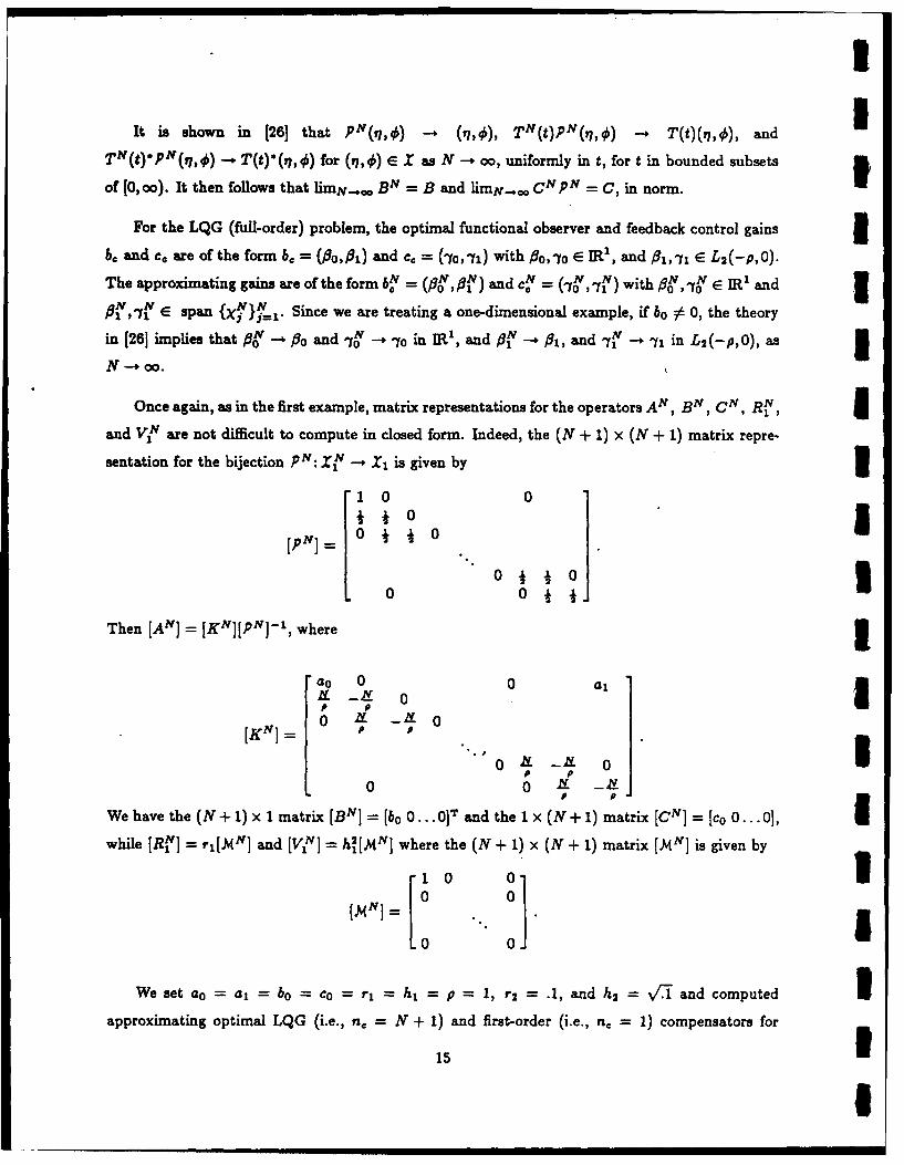
I

It is shown in [26] that pN(q,o) - (q,), TN(t)PN(h7q) .. T(t)(C7,q), and

TN(t)*PN(q,) - T(t)*(q, ) for (tq,4) E X as N --+ oo, uniformly in t, for t in bounded subsets

of [0,oo). It then follows that limN., BN = B and HImNCNPN = C, in norm.

For the LQG (full-order) problem, the optimal functional observer and feedback control gains 1b. and c. are of the form b, = (fo,P,) and c. = (i'o,i'i) with Po, -yo E IR', and 91, y, E L2(-p,0).

The approximating gains are of the form bN = ( N,N) and c = (-y, -I) with #N, -IN E IR1 and

E span {X} §1r Since we are treating a one-dimensional example, if bo 0 0, the theory

in [261 implies that #O -- o and 0yo' - -yo in IR, and PN --+ 91, and -yf -" "y in L 2(-p,0), as 300.

Once again, as in the first example, matrix representations for the operators AN, BN, CN, RN , 3and V N are not difficult to compute in closed form. Indeed, the (N + 1) x (N + 1) matrix repre-

sentation for the bijection p N: X N_- X1 is given by 31 0 0

I * 0Loo o I

LPI[ 0 0

Then [AN] - [K N][P/N]-, where Irao 0 0 alIt 0

[K I "" 0o !~

p pL 00o

We have the (N + 1) x 1 matrix [BNI = [bo 0...0 T and the 1 x (N + 1) matrix [CN] = [Co 0...0],

while [RN] = r, [AtN] and [VN] = h2 [.MN] where the (N + 1) x (N + 1) matrix [MN] is given by

1 0 0]

0 0

We set ao = a, = 50= co = r= hi = p = 1, r2 = .1, and h2 = Vf and computed Iapproximating optimal LQG (i.e., n, = N + 1) and first-order (i.e., n, = 1) compensators for

15

I

IN. 8,16,24, and 32. The optimal LQG observer gains are given in Table 3.3 and Figure 3.3; the

31 control gains are given in Table 3.4 and Figure 3.4. The first 23 open-loop poles of the system

(see (27]) are given in Table 3.2. The approximating first-order compensator gains along with the

31 corresponding and LQG closed-loop costs are given in Table 3.5 below. These costs were computed

using an evaluation model obtained by setting N = 64.. Note that the performance of the first-

order controllers is within 10% of the performance of the LQG controllers. Once again it is clear

that convergence is achieved.

1 1.278465

-1.588317 ± 4.155305i

-2.417631 ± 10.68603i

-2.861502 ± 17.05611i

-3.167754 ± 23.38558i

-3.401945 ± 29.69798i

-3.591627 ± 36.00146i

-3.751047 ± 42.29965i

3 -3.888543 ± 48.59442i

-4.009422 ± 54.88686i

3 -4.117267 + 61.17761i

-4.214618 - 67.46710iITable 3.2

1

| 16

I

S.0 .0 3

2...

Fiue 3.3

N. 8 1.2.3

#0 .234.422 4.2.*.43

Tal 3.3

170

D(ELAY COOINATE DELAY COJORDINtATE

-4 66 66 .0. G -.. -G.6. ,64 .6.0 *.a .0.9 66 - .6 0.6 .0.7 -. 0 .0.6 .6.4 -. 69 -. .0-.@.

.0.6 -. 6

-.. -..

.6.6 ..

Figur .3.4

3~ -441.4.422 -44234.23

TalU.OfLA COOOIMAC fl lAYCOOA!618

NIU

N Ac B,"cF JO J o

8 -4.835 -16.057 1.4042 1.5221 I16 -4.936 -16.343 1.403877 1.5298

24 -4.959 -16.378 1.403856 1.5309 332 -4.962 -16.404 1.403852 1.5317

Table 3.5 34. Summary and Concluding Remarks

We have proposed an approximation technique for computing optimal fixed-order compensators

for distributed parameter systems. Our approach involves using the optimal projection theory for

infinite-dimensional systems (which characterizes the optimal fixed-order compensator) developed Iin [181 in conjunction with finite-dimensional approximation of the infinite-dimensional plant. We

demonstrated the feasibility of our approach with two examples wherein we used spline-based Ritz- UGalerkin finite element schemes to compute approximating optimal first-order controllers for one-

dimensional, singe-input/output, parabolic (heat/diffusion) and hereditary control systems. Our 3numerical studies indicate that convergence of the compensator gains is achieved and that using

the first-order controller would lead to only minimal performance degradation over a standard LQG 3compensator while yielding significant implementation simplification.

At this point one is led naturally to ask the question of whether or not a satisfactory convergence Itheory could be developed. We are working on this at present and expect that such a theory

would conform closely in form and spirit to the convergence results for LQG approximation found lin [9] and [10] and outlined in Section 2 above. We also intend to consider our approximation

ideas in the context of discrete-time or sampled-data systems, and for continuous-time systems linvolving unbounded input and/or output (for example, boundary control systems), and systems

with control or measurement delays, see [11],[12]). Finally, we intend to investigate the application Iof our approximation framework to other infinite-dimensional control systems, in particular the

vibration control of flexible structures (i.e., second-order systems such as wave, beam, or plate 3equations).

Acknowledgment. The authors gratefully acknowledge Mr. S. W. Greeley, Mr. S. Richter, iand Mr. A. Daubendiek of Harris Corp. for carrying out the numerical computations reported in

Section 3. We also wish to thank Ms. J. M. Straehla, also of Harris Corp., for preparing the original Imanuscript in TEX.

19

I

References

1. Banks, H. T. and J. A. Burns, "Hereditary control problems: Numerical methods based on

averaging approximations," SIAM J. Control and Opt., 16, 169-208 (1978).

2. Gibson, J. S., "The Riccati integral equations for optimal control problems on Hilbert spaces,"SIAM J. Control and Opt., 17, 537-565 (1979).

3. Gibson, J. S., "An analysis of optimal modal regulation: Convergence and stability," SIAM J.Control and Opt., 19, 686-707 (1981).

4. Kunisch, K., "Approximation schemes for the linear quadratic optimal control problem asso-ciated with delay equations," SIAM J. Control and Opt., 20, 506-540 (1982).

5. Gibson, J. S., "Linear quadratic optimal control of hereditary differential systems: Infinitedimensional Riccati equations and numerical approximations," SIAM J. Control and Opt., 21,95-139 (1983).

6. Banks, H. T., I. G. Rosen, and K. Ito, "A spline based technique for computing Riccatioperators and feedback controls in regulator problems for delay equations," SIAM J. Sci.Stat. Comput., 5, 830-855 (1984).

7. Banks, H. T. and K. Kunisch, -The linear regulator problem for parabolic systems," SIAM J.Control and Opt., 22, 684-698 (1984).

8. Gibson, J. S. and I. G. Rosen, "Numerical approximation for the infinite dimensional discretetime optimal linear quadratic regulator problem," SIAM J. Control and Opt., 26, pp. 428-451(1988).

9. Gibson, J. S. and A. D. Adamian, "Approximation theory for LQG optimal control of flexiblestructures," Technical Report, Dept. Mech., Aero., Nuc. Eng., University of California, LosAngeles, CA, 1986.

10. Gibson, J. S. and I. G. Rosen, "Computational methods for optimal linear quadratic com-pensators for infinite dimensional discrete time systems," Proceedings of 3rd InternationalConference on Distributed Parameter Systems, Vorau, Austria, July 6-12, 1986, Lecture Notes3 in Control and Information Sciences No. 102, Springer-Verlag, New York, 1987, 120-135.

11. Gibson, J. S. and 1. G. Rosen, "Approximation of discrete time LQG compensators for dis-tributed systems with boundary input and unbounded measurement," Automatica, Vol. 23,3 1988.

12. Gibson, J. S. and I. G. Rosen, "Approximation in discrete time boundary control of flexiblestructures," Proceedings 26th IEEE Conference on Decision and Control, 535-540, Los Angeles,CA, Dec. 9-11, 1987.

13. Liu, Y. and B. D. 0. Anderson, "Controller reduction via stable factorization and balancing,"Int. J. Control, 44, 507-531 (1986).

14. Hyland, D. C. and D. S. Bernstein, "The optimal projection equations for fixed-order dynamiccompensation," IEEE Trans. Auto. Contr., AC-29, 1034-1037, (1984).

15. Johnson, T. L., "Optimization of low order compensators for infinite dimensional systems,"Proc. 9th IFIP Symposium on Optimization Techniques, Warsaw, Poland, September, 1979,394-401.

16. Pearson, R. K., "Optimal fixed form compensators for large space structures," in A COSSSix (Active Control of Space Structures), RADC-TR-81-289, Rome Air Development Center,Griffiss Air Force Base, New York, 1981.3

I

I3

II

17. Johnson, T. L., "Progress in modelling and control of flexible spacecraft," J. Franklin Inst.,315, 495-520 (1983).

18. Bernstein, D. S. and D. C. Hyland, "The optimal projection equations for finite-dimensionalfixed-order dynamic compensation of infinite dimensional systems," SIAM J. Control and Opt.,24, 122-151 (1986).

19. Richter, S., "A homotopy algorithm for solving the optimal projection equations for fixedorder dynamic compensation of infinite dimensional systems," SIAM J. Control and Opt., 24,122-151 (1986).

20. Greeley, S. W. and D. C. Hyland, "Reduced order compensation: LQG reduction versus opti-mal projection using a homotopic continuation method," Proc. IEEE Conference on Decisionand Control, Los Angeles, CA, Dec. 9-11, 1987, 742-747.

21. Curtain, R. F. and A. J. Pritchard, Infinite Dimensional Linear Systems Theory, Springer-Verlag, New York, 1978.

22. Balakrishnan, A. V., Applied Functional Analysis, Springer-Verlag, New York, 1981.23. Pazy, A., Semigroups of Linear Operators and Applications to Partial Differential Equations,

Springer- Verlag, New York, 1983.24. Smith, M. C., "On minimal order stabilization of single loop plants," Sys. Contr. Letters, 7, 3

39-40 (1986).25. Swartz, B. K. and R. S. Varga, "Error bounds for spline and L-spline interpolation," J. Approx.

Theory, 6, 6-49 (1972).I26. Ito, K. and F. Kappel, "A uniformly differentiable approximation scheme for delay systems

using splines," Technical Report 87-94, Institute fur Mathematik, Technische Universitat Grazand Universitat Graz, Graz, Austria, 1987, and Appl. Math. Optim., submitted.

27. Ito, K., "On the approximation of eigenvalues associated with functional differential equations,"J. Diff. Equ., 60, 285-300 (1985). 1

IUaUIIII

II

IIIIUI'

5 APPMndIX D: Decentralized Control

76. D. S. Bernstein, "Sequential Design of Decentralized DynamicCoensators Using the Optimal Projection Equations," Int. J. Contr.,Vol. 46, pp. 1569-1577, 1987.

121. D. S. Bernstein and W. M. Haddad, "Robust Decentralized Static OutputFeedback," submitted to Sys. Contr. Lett.

IIIII!

III

I

tNT. J. CONTROL, 1987, VOL. 46, NO. 5, 1569-1577

3 Sequential design of decentralized dynamic compensators using theoptimal projection equations

3 DENNIS S. BERNSTEINt

The optimal projection equations for quadratically optimal centralized fixed-orderdynamic compensation are generalized to the case in which the dynamic com-pensator has, in addition, a fixed decentralized structure. Under a stabilizabilityassumption for the particular feedback configuration, the resulting optimalityconditions explicitly characterize each subcontroller in terms of the plant andremaining subcontrollers. This characterization associates an oblique projectionwith each subcontroller and suggests an iterative sequential design algorithm. Theres,,lts are applied to an interconnected flexible beam example.

I 1. IntroductionThe purpose of this note is to consider the problem of designing decentralized

dynamic feedback controllers using recently obtained results on quadratically optimalfixed-order dynamic compensation (Hyland and Bernstein 1984). As in Bernussouand Titli (1982). Looze et al. (1978), and Singh (1981), the overall approach is to fix thestructure (information pattern and order) of the linear controller and optimize the

steady-state regulation cost with respect to the controller parameters. The underlyingphilosophy is that the ability to carry out such an optimization procedure permits theevaluation of a particular decentralized configuration which may be dictated byimplementation constraints. If there is some flexibility in designing the decentralizedarchitecture, then these results can be used to evaluate the optimal performance ofeach permissible configuration, and hence to determine preferable structures. Sincethe present paper is confined to the question of optimal regulation, trade-offs withrt ard to robustness in the presence of plant variations are not considered. Suchtrade-offs can be included, however, by utilizing the Stratonovich multiplicative whitenoise approach developed by Bernstein and Hyland (1985).

To further motivate our approach, consider the problem of controlling an nth-order plant Y by means of a decentralized dynamic compensator consisting ofsubcontrollers W, and W2. A straightforward design technique that immediatelycomes to mind is that of sequential optimization (Davison and Gesing 1979, Jamshidi1983). To begin, ignore W2 and design W, as a centralized controller for *. Next,regard the closed-loop system consisting of Y and W, as an augmented system Y anddesign 'W' as a centralized controller for JY. Now redesign W, to be a centralizedcontroller for the augmented closed-loop system composed of Y and W¢2, and so forth.One difficulty with this scheme, however, is that of dimension. If, for example, one wereto employ LQG at each step of this algorithm, then on the first iteration W, wouldhave dimension n and thus W2 would have dimension 2n. On the second iteration, Wtwould require dimension 3n and W2 would have order 4n, and so forth. Such

Received 15 December 1986.t Harris Corporation, Government Aerospace Systems Division, P.O. Box 94000,

Melbourne, Florida 32902, U.S.A.

II

II

1570 D. S. Bernstein

difficulties can be avoided by setting n = 0, which essentially corresponds to staticoutput feedback. Although easier to implement, static output feedback jacks filteringabilities such as are inherent in LQG controllers, which are purely dyn1mie (i.e. strictlypreper).

As discussed by Sandell et al. (1978), p. 119, the explanation for this difficulty isprovided by the 'second-guessing' phenomenon: when LQG is used, each subcon-troller must consist of linear feedback, not only of estimates of the plant states but alsoof estimates of the other subcontrollers' estimates. Hence the 'optimal' controller is Igiven by an irrational transfer function, i.e. a distributed parameter (infinite-dimensional) system. Such controllers, of course, must be ruled out since their designand implementation (except in special cases) violate physical realizability (see, forexample, Bernstein and Hyland 1986). U

Having thus ruled out zeroth-order and infinite-order decentralized controllers,we focus on the problem of designing purely dynamic decentralized compensators.Moreover, by invoking the constraint of fixed subcontroller order, we overcome thesecond-guessing phenomenon. Utilizing the parameter optimization approach thusleads to a generalization of the result obtained by Hyland and Bernstein (1984) forcentralized control. In brief, it was shown in Hyland and Bernstein (1984) that theunwieldy first-order necessary conditions for fixed-order dynamic compensation canbe simplified by exploiting the presence of a previously unrecognized obliqueprojection. The resulting optimal projection equations, which consist of a pair ofmodified Riccati equations and a pair of modified Lyapunov equations coupled by the Ioptimal projection, yield insight into the structure of the optimal dynamic com-pensator and emphasize the breakdown of the separation principle for reduced-ordercontroller design. For example, the optimal compensator is the projection of a full- Iorder dynamic controller which is generally different from the LQG design.Furthermore, this full-order controller and the oblique projection are intricatelyrelated since they are simultaneously determined by the coupled design equations. Animmediate consequence is the observation that stepwise schemes employing either Imodel reduction followed by LQG or LQG followed by model reduction are generallysuboptimal. For computational purposes, the optimal projection equations permit thedevelopment of novel numerical methods which operate through successive iteration Iof the oblique projectic . (Hyland and Bernstein 1985). Such algorithms are thusphilosophically and operationally distinct from gradient search methods.

The generalization of the optimal projection equations to the decentralized case isstraightforward and immediate. In the optimization process each subcontroller is Iviewed as a centralized controller for an augmented 'plant' consisting of the actualplant and all other subcontrollers. It need only be observed that the necessaryconditions for optimality for the decentralized problem must consist of the collection Iof necessary conditions obtained by optimizing over each subcontroller separatelywhile keeping the other subcontrollers fixed. More precisely, this statement corre-sponds to the fact that setting the Frechet derivative to zero is equivalent to setting theindividual partial derivatives to zero. Hence it is not surprising that the optimalprojection tuations for the decentralized problem involve multiple oblique projec-tions, one associated with each subcontroller. Furthermore, each subcontrollerincorporates an internal model (in the sense of an oblique projection of full-order Idynamics) not only of the plant but also of all other subcontrollers. The structure ofthe equations suggests a sequential design algorithm such as that proposed in thiswork.

1I

• . a l l l lI II

IDesign of decentralized dynamic compensators 1571

3 The simplicity with which this result is obtained should not belie its relevance tothe decentralized control problem. Specifically, our approach is distinct from sub-system-decomposition techniques (Ikeda and Siljak 1980, 1981, Ikeda et al. 1981,1984, Lindner 1985, Linnemann 1984, Ozguner 1979, Ramakrishna and Viswanadham1982, Saeks 1979, Sezer and Huseyin 1984, Silkak 1978, 1983) and model-reductionmethods since the optimal projection equations retain the full, interconnectedplant at all times. For the proposed algorithm, decomposition techniques whichexploit subsystem-interconnection data can play a role by providing a starting pointfor subsequent iterative refinement and optimization. Decomposition methods mayalso play a role when very high dimensionality precludes direct solution of the optimalprojection equations. These are areas for future research.

With regard to the role of the oblique projection, it should be noted that suchtransformations do not, in general, preserve plant characteristics such as poles, zeros,subspaces, etc. Indeed, since the oblique projection arises as a consequence ofoptimality, approaches that seek to retain system invariants (e.g. Uskokovic andMedanic 1985) are generally suboptimal. In addition, the comrplex coupling amongthe plant and subcontrollers via multiple oblique projections provides an additionalmeasure for evaluating the suboptimality of the methods proposed.

The plan of the paper is as follows. The fixed-structure decentralized dynamic-compensation problem is stated in § 2 along with the generalization of the optimalprojection equations. In § 3 we propose a sequential design algorithm for solving theseequations and state conditions under which convergence is guaranteed. Finally, in § 4the algorithm is applied to the 8th-order model of a pair of simply supported beamsconnected by a spring. For this example, we obtain a two-channel decentralizeddesign which is 4th-order in each channel and compare its performance with the (8th-order) centralized LQG design.

3 2. Problem statement and main theorem

Given the controlled system

3 )(t) tAx() + i Biu1(t) + wo(t) (2.1)

yi(t) Cix(t) + wi(t), i =. p (2.2)

design a fixed-structure decentralized dynamic compensator

, xi(t)=A~jxci(t) + Bgiy,(t), i- 1....p (2.3)

u1(t) =Ccx (t), i= 1....p (2.4)

which minimizes the steady-state performance criterion

J(A 1, B, 1, CC ,, B,,, C,,) Alim EIF X(t)T ROx(t) + Ui (t)T Riui(t)1 (2.5)L

3 where, for i= 1. p: x eP, u Em ' , y E P", c,,ER" -, nc _ 4 n,, ni<5n + nc-n,,.i-I

A, Bi, C, Ac,, Be, C,,, Ro and Ri are matrices of appropriate dimension with Ro(symmetric) non-negative definite and R (symmetric) positive definite; wo is whitedisturbance noise with n x n non-negative-definite intensity V, and w, is white

UI

1572 D. S. Bernstein 3observation noise with i x Ii positive-definite intensity V, where w, , w,,..., w, aremutually uncorrelated and have zero mean. E denotes expectation and superscript Tindicates transpose.

To guarantee that J is finite and independent of initial conditions we restrict ourattention to the set of admissible stabilizing compensators

.- {(A.,, B. 1, C.l1 , .., A,,, B,,, C,,): ,4 is asymptotically stable}

where the closed-loop dynamics matrix J is given by 3

where

I- -] IC/C,

LCP

A, block-diagonal (A,,..... ACP) IB, - block-diagonal (B,,,..., Bc')

C, A block-diagonal (C 1 ,...,C) 3(For possibly non-square matrices S1 , S2, block-diagonal (S,, S2) denotes the

matrix [S' S])

It is possible that for certain decentralized structures the system is nut stabilizable, Ii.e. d is empty (Wang and Davison 1973, Seraji 1982, Sezer and Siljak 1981). Ourapproach, however, is to assume that dl is not empty and characterize the optimaldecentralized controller over the stabilizing class. Since the value of J is independentof the internal realization of each subcompensator, without loss of generality we canfurther restrict our attention to

S/+ {(Ac 1, B, 1 , C 1,..., Acp, BP, Ce.p) c. sY: (Ac1 , Bcj) is controllable and 3(Cc1 , Aci) is observable, i = 1. p}

The following lemma is an immediate consequence of Theorem 6.2.5, p. 123 of Raoand Mitra (1971). Let 1, denote the r x r identity matrix.

Lemma 2.1 1Suppose , 5 E 9 - 9 are non-negative definite and rank Q r. Then there exist

G, r e PFq and invertible M e '" such that

OP = GrMr (2.6) 3rG T=I, (2.7)

For convenience in stating the main theorem, call (G, M, ) satisfying (2.6), (2.7) a UUU

Design of decentralized dynamic compensators 1573

projective factorization of 015. Such a factorization is unique modulo an arbitrarychange in basis in P', which corresponds to nothing more than a change of basis forthe internal representation of the compensator (or subcompensators in the presentcontext).

We shall also require the following notation. Let i denote AZ with the rows andcolumns containing AC, deleted. Similarly, let 1 be obtained by deleting the rows and3 columns corresponding to C'RiCcE in the matrix

, block-diagonal (Ro, Cc' RI Cc CP P

iAnd furthermore, Pi is obtained by deleting the rows and columns containing Bci ViB cin

A block-diagonal (VB,, B T B,, , B T

Also define C1 BP

100. - Rc) . ,/

where 0,.., denotes the r x s zero matrix. Note that il fi, C,, , and 1 essentiallyrepresent the closed-loop system minus the ith subcontroller as controlled by thelatter. Finally, define

and, for T e P"F', let

I r~~, -t --

Main theoremSuppose (A 1, B 1,Cc1, .... AcP, B, C0P , ) s,+1 solves the steady-state fixed-

structure decentralized dynamic-compensation problem. Then for i = 1, ..., p thereexist (n + n, - n,,) x (n + n, - nci) non-negative-definite matrices Q,, Pi, Qi and Pisuch that A0 i, Bi and Ci are given by

3 Azi = ri(A - QiFi - 7lPi)G (2.8)

Bci = FiQ Ti vi- (2.9)

3 C,, = - Ri'§TPiG (2.10)

for some projective factorization G,, M,, ri of O1 P1 , and such that, with T, GT r,, thefollowing conditions are satisfied:

0 = A, Q , + 0.,2 + R - Q, E Q, + Ti, Q.,Zi ,P.,i. (2.11)

0=iAPL+ PAi+ -PPL+*,P P, (2.12)I 0 = (A, - EIP,)Q - A- P) + Q,!,Q, - .QE1Qf, (2.13)

0 = ('4' _ QyE)T5, + P,(Ai _ QE,) + plp _ TT PtPiz, (2.14)

U rank (=rankf 1 = rank i Pi = nci (2.15)

UU

I

1574 D. S. Bernstein iRemark 2.1

Because of (2.7) the matrix T, is idempotent, i.e. rj = i. This projection corre- 3sponding to the ith subcontroller is an oblique projection (as opposed to anorthogonal projection) since it is not necessarily symmetric. Furthermore, T, is given inclosed form by ll

_ 1where ( )I denotes the (Drazin) group generalized inverse (see, for example, Campbelland Meyer, 1979, p. 124). I3. Proposed algorithmSequential design algorithm

Step 1. Choose a starting point consisting of initial subcontroller designs;Step 2. For a sequence {i4} 1=,, where ik e{1 ... , p), k = 1, 2., redesign subcon-

troller i, as an optimal fixed-order centralized controller for the plant and Iremaining subcontrollers;

Step 3. Compute the cost J, of the current design and check Jk - J_ 1 forconvergence.

Note that the first two steps of the algorithm consist of (i) bringing suboptimalsubcontrollers 'on line' and (ii) iteratively refining each subcontroller. As discussed in§ 1, the choice of a starting design for Step 1 can be obtained by a variety of existingmethods such as subsystem decomposition. As for subcontrolfer refinement, note thateach subcontroller redesign procedure is equivalent to replacing a suboptimalsubcontroller with a subcontroller which is optimal with respect to the plant and Iremaining subcontrollers.

Proposition 3.1 3For a given starting design and redesign sequence { ik } " suppose that the optimal

projection equations can be solved for each k to yield the global minimum. Then{f J }, is monotonically non-increasing and hence convergent.

Determining both a suitable starting point and redesign sequence for solvabilityand attaining the decentralized global minimum remain areas for future research.With regard to algorithms for solving the optimal projection equations for each Isubcontroller redesign procedure, details of proposed algorithms can be found in theworks of Hyland (1983, 1984) and Hyland and Bernstein (1985).

4. Application to interconnected flexible beamsTo demonstrate the applicability of the main theorem and the sequential design

algorithm, we consider a pair of simply supported Euler-Bernoulli flexible beams 1interconnected by a spring (see the Figure). Each beam possesses one rate sensor andone force actuator. Retaining two vibrational modes in each beam, we obtain the 8th-order interconnected model 3

A A , A2, , B 11 J B2 04 x I

LA 21 A22 °J L B22 I

C1 =[CI 1 0,], C2 =[01. 4 C22 ] 3II

IiI

Design of decentralized dynamic compensators 1575

III

U where

I 0oli 0 0 1- coI-(k/o I)(sin rci) 2 -2jioj -(k/cu 2j(sin irci)(sin 2irc1 ) 0

A0 - -0 0,2

-(k/cli)(sin 7ci)(sin 27rci) 0 -t 2 1 - (k/wl2 1)(sin 27rc )2 -2CoJ21

3[0 0 0 01Aj = (k/cowj)(sin ci)(sin ncj) 0 (k/wo2j)(sin 7rci)(sin 21rcj) 0

I 0 0 0

(k/wo1 j)(sin 7rcj)(sin 21rci) 0 (k/W2j)(sin 21ci))(sin 27tc,) 03 i#j

F01sinf 7ra1

B 0= , = [0 sin 7rsi 0 sin 2ns]

-sin 2na j

aI = dIL,. si = §1lL, cj = elLi

In the above definitions, k is the spring constant, coj, is the jth modal frequency of theith beam, C, is the damping ratio of the ith beam, L is the length of the ith beam, anda1, 9, and e, are, respectively, the actuator, sensor and spring-connection coordinatesas measured from the left in the Figure. The chosen values areU

U

I1576 D. S. Bernstein

k= 10 3woi=l, w2=4, Ci=O0005, Li=, i=1,2

d, = 0"3, 9, = 0-65, e, =06 3J2 = 0-8, s2 = 0"2, e2 = 0-4

In addition, weighting and intensity matrices are chosen to be

R, = block-diagonal 0 [(I I/ J1 / l21]' [0 1/o012]' 1/1 1221)

R2 = R3 =0.112

Vo=block-diagonal([ 0i,0 0 0]'[I 0 0],[0 )

V = V2 = 0.112

For this problem the open-loop cost was evaluated and the centralized 8th-orderLQG design was obtained to provide a baseline. To provide a starting point for thesequential design algorithm, a pair of 4th-order LQG controllers were designed foreach beam separately ignoring the interconnection, i.e. setting k = 0. The optimal Iprojection equations were then utilized to iteratively refine each subcontroller. Theresults are summarized in the Table.

Design Cost

Open loop 163"5Centralized LQG

n.. = 8 19.99Suboptimal decentralized

nc, n.2 -- 4 59.43Redesign subcontroller 2 28.19Redesign subcontroller 1 23.29Redesign subcontroller 2 23.04Redesign subcontroller 1 22.25 IRedesign subcontroller 2 21.94Redesign subcontroller 1 21-86Redesign subcontroller 2 21.81Redesign subcontroller 1 21-79

ACKNOWLEDGMENTS UThis research was supported in part by the Air Force Office of Scientific Research

under contracts F49620-86-C-0002 and F49620-86-C-0038.The author wishes to thank Scott W. Greeley for providing the beam model in § 4

and for carrying out the design computations. UU3

Design of decentralized dynamic cornpensators 1577

REFERENcEsI BERNSTEIN, D. S., and HYLAND, D. C., 1985, Proc. 24th I.E.E.E. Conf. Dec. Control, 745; 1986,SIAM J1 Control Optim., 24, 122.

BERNUSSOU, J., and Trni, A., 1982, Interconnected Dynamical Systems: Stability, DecompositionI and Decentralization (New York: North-Holland).CAMPBELL, S. L., and MEYER, C. D., Jr., 1979, Generalized Inverses of Linear Transformations

(London: Pitman).DAVISON, E. J., and GESING, W., 1979, Autoinatica, 15, 307.DE CARLO, R. A., and SAEKs, R., 1981, Interconnected Dynamical Systems (New York: Marcel

HYLAND, D. C., 1983, AIAA 21st Aerospace Sciences Meeting, paper 83-0303; 1984, Proc. AIAADynamics Specialists Conf., 381.

HYLAND, D. C., and BERNSTEIN, D. S., 1984, I.E.E.E. Trans. autom. Control, 29, 1034; 1985, Ibid.,

IKEDA, M., and SIUAK, D. D., 1980, Large-scale Syst., 1, 29; 1981, I.E.E.E. Trans. autom. Control,26, 1118.

IKEDA, M., SILJAK, D. D., and WHITE, D. E., 1981, J. optim. Theory Applic., 34, 279; 1984,I I.E.E.E. Trans. autom. Control, 29, 244.JAMSHIDI, M., 1983, Large-Scale Systems (New York: North-Holland).LINDNER, D. K., 1985, Syst. Control Lett., 6, 109.LINNEMANN, A., 1984, I.E.E.E. Trans. autom. Control, 29, 1052.I LoozE, D. P., HouPr, P. K., SANDELL, N. R., and ATHANS, M., 1978, I.E.E.E. Trans. autom. Control,

23, 268.OZGUNER, U., 1979, I.E.E.E. Trans. autom. Control, 24, 652.RAMAKRISHNA, A., and VISWANADHAM, N., 1982, I.E.E.E. Trans. autom. Control, 27, 159.RAO, C. R., and MiRrpA, S. K., 1971, Generalized Inverse of Matrices and its Applications (New

SAEKS, R., 1979, I.E.E.E. Trans. autom. Control, 24, 269.SANDELL, N., VARAIYA, P., ATHANS, M., and SAFONOV, M. G., 1978, I.E.E.E. Trans. autom.

Control. 23, 108.SERxI H., 1982, Int. J. Control, 35, 775.SEZER, M. E., and HUSEYIN, 0., 1984, Automatica, 16, 205.SEZER, M. E., and SIUAK, D. D., 1981, Syst. Control Lett., 1, 60.SILJAK, D. D., 1978, Large Scale Dynamic Systems (New York: North-Holland); 1983, Large-

SINGH, M. G., 1981, Decentralised Control (New York: North-Holland).USKoicOVIC, Z., and MEDANIC, J., 1985, Proc. 24th I.E.E.E. Conf. on Decision and Control, 837.I WANG, S. H., and DAVISON, E. .J., 1973, I.E.E.E. Trans. autom. Control, 18, 473.

II

April 1988II3 Robust Decentralized Output Feedback:

The Static Controller Case

IUI

by

IIDennis S. Bernstein Wassim M. Haddad

Harris Corporation Department of Mechanical andGovernment Aerospace Systems Division Aerospace Engineering

MS 22/4848 Florida Institute of TechnologyMelbourne, FL 32902 Melbourne, FL 32'.JI

U Keywords: robust, guaranteed bounds, optimal, structured uncertainty, real parameters

Abstract

Sufficient conditions are developed for designing robust decentralized static output feedbackcontrollers. The approach involves deriving necessary conditions for minimizing a bound on closed-loop performance over - specified range of uncertain parameters. The effect of plant parametervariations on the closed-loop covariance is overbounded by means of a modified Lyapunov equationwhose solutions are guaranteed to provide robust stability and performance.3

ISupported in part by the Air Force Office of Scientific Research under contract F49620-86-C-

0038.

1

II

1. Introduction

Because of implementation constraints, cost, and reliability considerations, a decentralized 1

controller architecture is often required for controlling large scale systems. Furthermore, such

controllers must be robust to variations in plant parameters. The present paper addresses both I

of these concerns within the context of a robust decentralized theory for continuous-time static

controllers. 3The approach to controller design considered herein involves optimizing closed-loop perfor- I

mance with respect to the feedback gains. This approach to output feedback was studied for

centralized controllers in [8,91 and for decentralized controllers in [10]. An interesting feature of

[9,101 is the recognition of an oblique projection (idempotent matrix) which allows the necessary 1

conditions to be written in terms of a modified Riccati equation. When the problem is specialized

to full-state feedback, the projection becomes the identity and the modified Riccati equation coin- 1cides with the standard Riccati equation of LQR theory. It should be pointed out that this oblique

projection is distinct from the oblique projection arising in dynamic compensation ([7]). A unified 1treatment of the static/dynamic (nonstrictly proper) centralized control problem involving both

projections is given in [2]. 3The present paper goes beyond earlier work by deriving sufficient conditions for robust stability

and performance with respect to variations in the plant parameters. Although plant disturbances

are represented in the usual stochastic manner by means of additive white noise, uncertainty in the

plant dynamics is modeled deterministically by means of constant structured parameter variations 1within bounded sets. Thus, for example, the dynamics matrix A is replaced by A + I

where ak is a constant uncertain parameter assumed only to lie within the interval [- ca, ak but 3otherwise unknown, and Ak is a fixed matrix denoting the structure of the uncertain parameter

ak as it appears in the nominal dynamics matrix A. The system performance is defined to be the Iworst-case value over the class of parameter uncertainties of a quadratic criterion averaged over the

disturbance statistics. 3Since the closed-loop performance can be written in terms of the second-moment matrix, a

performance bound over the class of uncertain parameters can be obtained by bounding the state

covariance. The key to bounding the state covariance is to replace the usual Lyapunov equation for

the second-moment matrix by a modified Lyapunov equation. In the present paper the modified 1Lyapunov equation is constructed by adding two additional terms. The first term corresponds to aII

1 3II1

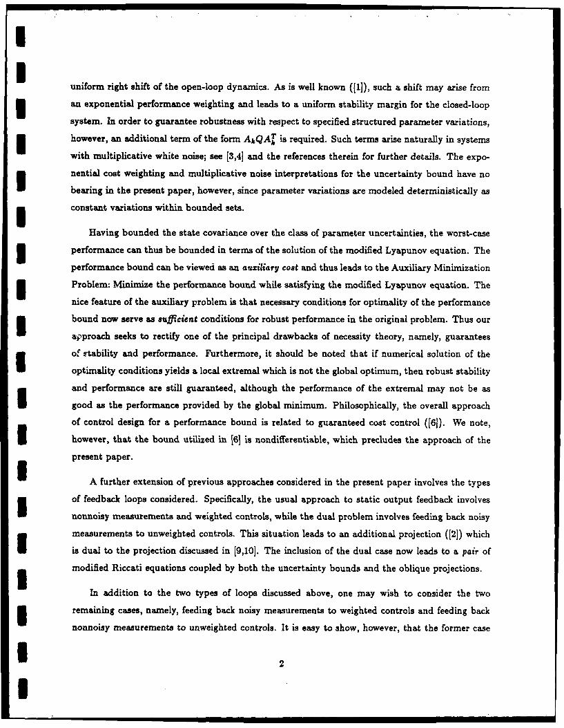
uniform right shift of the open-loop dynamics. As is well known ([1]), such a shift may arise from3 an exponential performance weighting and leads to a uniform stability margin for the closed-loop

system. In order to guarantee robustness with respect to specified structured parameter variations,

however, an additional term of the form AkQAT is required. Such terms arise naturally in systems

with multiplicative white noise; see [3,4] and the references therein for further details. The expo-

nential cost weighting and multiplicative noise interpretations for the uncertainty bound have no

bearing in the present paper, however, since parameter variations are modeled deterministically as

constant variations within bounded sets.

Having bounded the state covariance over the class of parameter uncertainties, the worst-case

3 performance can thus be bounded in terms of the solution of the modified Lyapunov equation. The

performance bound can be viewed as an auxiliary cost and thus leads to the Auxiliary Minimization

5 Problem: Minimize the performance bound while satisfying the modified Lyapunov equation. The

nice feature of the auxiliary problem is that necessary conditions for optimality of the performance

bound now serve as sufficient conditions for robust performance in the original problem. Thus our

approach seeks to rectify one of the principal drawbacks of necessity theory, namely, guarantees

of rtability and performance. Furthermore, it should be noted that if numerical solution of the

optimality conditions yields a local extremal which is not the global optimum, then robust stability

and performance are still guaranteed, although the performance of the extremal may not be as

good as the performance provided by the global minimum. Philosophically, the overall approach

of control design for a performance bound is related to guaranteed cost control ([6]). We note,

however, that the bound utilized in [6] is nondifferentiable, which precludes the approach of the

present paper.

A further extension of previous approaches considered in the present paper involves the types

of feedback loops considered. Specifically, the usual approach to static output feedback involves

nonnoisy measurements and weighted controls, while the dual problem involves feeding back noisy

measurements to unweighted controls. This situation leads to an additional projection ([21) which

is dual to the projection discussed in [9,10]. The inclusion of the dual case now leads to a pair of

modified Riccati equations coupled by both the uncertainty bounds and the oblique projections.

In addition to the two types of loops discussed above, one may wish to consider the two

3 remaining cases, namely, feeding back noisy measurements to weighted controls and feeding back

nonnoisy measurements to unweighted controls. It is easy to show, however, that the former case

I .2

I1

leads to an undefined (i.e., infinite) value for the performance while the latter case is highly singular

and thus will not be treated here.

Finally, the scope of the present paper is limited to the development of sufficient conditions for

robust decentralized output feedback. Numerical solution of these equations can be carried out by 3extending available algorithms for centralized output feedback. Numerical algorithms for solving a

single modified Riccati equation in the absence of uncertainty bounds are discussed in [101. 32. Notation and DefinitionsIR, IRJx , IRr, IE real numbers, r x s real numbers, IR'xI, expectation 1

I,, ( )T r x r identity, transpose

ED, 9 Kronecker sum, Kronecker product ([51)Sr r x r symmetric matrices

INr r x r symmetric nonnegative-definite matrices

IP' r x r symmetric positive-definite matrices IZ2 <5 Z2 Z2 - Z E IN , Z 1,Z2 E SrZ1 < Z2 Z2 - Zi E IPr, Z, Z2 E Sr

asymptotically matrix with eigenvalues in open left half plane Istable matrix

n, r, s, p positive integers 3i,j.k indices, i=1,...,r, j=1,..°,s, k-=1,...,p

Mi, . positive integers, i = I,..., r

rhy, 4j positive integers, j= 1,...,s IZ n-dimensional vector

ui, it in, 4-dimensional vectors, i = 1,..., r

ui, Yj rhj, 4j-dimensional vectors, j I,..., s

A, AA n x n matrices

Bi,AB1 ;C, n x mi matrices; 4 x n matrices, i = l,...,r 3by;C,, ACj n x th. matrices; tj x n matrices, j= 1,...,s

Al nxnmatrices, k=1,...p

Bk n x ri matrices, i =1,...,r, k=1,...,p IC j k t4 x n matrices, 1= 1,...,, k=1,...,p

m -x4matrices, i=1,...,r 3Ecj rhi" x tj matrices, j = ,...,s

a positive number

A, A+ Zak positive number, k = 1,...,p

^k a/a, k=1,...,p I

ak real number, k = 1,...,pw0(t), Wj(t) n-dimensional, te-dimensional white noise, j = 1,... , s

3

U

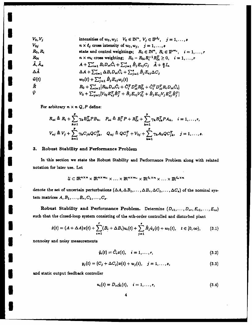
VoVj ~~intensities Of Wo,WY-; VoI, i P , l..,VveN, Vj1Pj ......a

i ~Voi n x ii cross intensity of wo, wj, --1.,s

Ro, RI state and control weightings; Ro E INn , R?.e Ip,, i- ,. rR0, n x mi cross weighting; Ro-Ro.R7R >O, t=1,...,r5 AAa A +E j BjD66ji+E hz-E -3 C- A + in

AA + E7 ABDjIIC + Z@= b3 EC,&Cj3 t (t) t(t) + h3E 0= 3W(t)Ro + Er ,I.RoD, + 6T T

VVo + f,[V 0 "E,. 3. + B1 Ee1 V02 + BjEcVE.TBT

For arbitrary n x n Q, P define:

R., R+- kBTPB., P., YBP+R.+E- r B PAk,

k=1 k=1

tk kZ j Q, A iQCT+ Voi +ZE'mAkAQCj, j=:I...,.h=1 k=1

3. Robust Stability and Performance Problem

5In this section we state the Robust Stability and Performance Problem along with related

notation for later use. Let

U C IRnXnX IRnXm i X ... X IRn xth x IR1- x X ... X R '*xn

denote the set of uncertain perturbations (AA, ABI,..., AB,, AC,,..., AC.) of the nominal sys-

tem matrices A, B,...,B, C1 ,... ,C.

Robust Stability and Performance Problem. Determine (D 1,, ... ,D rEc..,EC8)

such that the closed-loop system consisting of the nth-order controlled and disturbed plant

r a

i (t) = (A + AA)x(t) + E B+ AB1 )u,(t) + ~flaj(t)+ Wo(t), t E[0Ooo), (3.1)i=1 j=1

3 nonnoisy and noisy measurements

j,(t) = 6i, (t), i = r,. , (3.2)

y3(t) = (C + AC)z(t) + W(t), j = 1,...,s, (3.3)

3 and static output feedback controller

u,(t) = Dji(t), i = 1,...,, (3.4)

4

1

I

f =(t) Eciyj(t), j = 1,...,a, (3.5)

is asymptotically stable for all variations in U and the performance criterion 3J(Del*I,.. ,De,,Eels .,IEs)A

sup limsup IE[zT(t) az(t) + 2ZXTt)Rou, (t) + u(t)Riu,(,)] (3.6)U t- =1 1=1

is minimized. 3For each controller (De,,.. ., Der, Eel,..., E,,) and variation in U, the closed-loop system (3.1)-

(3.5) is given by I= (i+ tE [0,o), (3.7)

where tii(t) is white noise with intensity V" E IN'. 3Remark 3.1. In the case AA, ABj,ACI = 0 it is well known that stabilizability is related to 3

the existence of fixed modes ([111). When plant uncertainties are present the problem is, of course,

far more complex. In the present paper sufficient conditions for robust stability are obtained as a 3consequence of the existence of robust performance bounds.

Remark 3.2. Note that the controller architecture is quite general in that it includes two 3distinctly different types of decentralized loops. The first type, indexed by i - 1,..., r, involves

feeding back nonnoisy measurements to weighted controls. This is the standard setting in the

optimal output-feedback literature ([8-10]). In addition, we include the dual situation, indexed by

j = 1,..., a, which involves feeding back noisy measurements to iinweighted controls. The case in 3which only one type of loop is present can be formally recovered from our results by ignoring B,

and di or B., and Cj as required. As noted in Section 1, noisy measurements cannot be fed back

to weighted controls via static control, while feeding back nonnoisy measurements to unweighted

controls is a singular problem.

Remark 3.3. Note that the problem statement is restrictive in the sense that uncertainties

in both the control and observation matrices are not permitted within the same feedback loop. 3Although it is indeed possible to permit such simultaneous uncertainties, the development is con-

siderably more complex and hence is not treated here. 3Remark 3.4. The cost functional (3.6) is identical to the LQG criterion (usually stated in

terms of an averaged integral) with the exception of the supremum for evaluating worst case over IU. 5

U

I4. Sufficient Conditions for Robust Stability and Performance

I In practice, steady-state performance is only of interest when the closed-loop system (3.7)

is stable over U. The following result, which expresses the performance in terms of the state

I covariance, is immediate.

3 Lemma% 4.1. Let (Dm,,... y Der Ee,..., E=.) be given and suppose the system (3.7) is stable

for all variations in U. Then

J(Del,..., D el ,..., Emr) = sup tr Q& A, (4.1)U

where Q, -A lim...o I.[x(t)xT(t)] E IN' is the unique solution to

0 = (A + AA)Q+qA (A + .A)r + f. (4.2)

Remark 4.1. When U is compact, 'sup* in (4.1) can be replaced by "max".

We now seek upper bounds for J(Dl,...,D47,E=,,...,Ee.). Our assumptions allow us to

obtain robust stability as a consequence of robust performance.

Theorem 4.1. Let 2 : iN' x IR l mmx x I , xL1 x ... x IRA. x t" --4 Sn be such

* that

,&,Q + Q,&T < n(Q, Del,...., Da,, Eal,,..., PEo),I (A, AB,...AB,%C,,.., %Ce U,I

(Q, Dell...,IDer,,Eel,... IE,) C INn x 1R ,,, x", x ... x IR ' i x IRA I x L x ... x IRA-' x

I (4.3)

Furthermore, for given (D 1,... , D,, Ee,,... , E..) suppose there exists Q E INn satisfying

I0 = AQ + QAT +/t(Q, Dell ..., Der, Eel, .... E..) + .(4.4)

3 Then the pair (A + AA,'V) is stabilizable for all variations in U if and only if A + A is asymp-

totically stable for all variations in U. In this case,

I QA Q, (4.5)

3 where Q,&, satisfies (4.2), and

3 J(Dc,,..., Der, E,...,Ec.) < tr QR. (4.6)

6I

I

Proof. For all variations in U, (4.4) is equivalent to U0 (A +AA)Q + Q( + AA)T + (Q, D,,,..., Dr, EI,... E,, A-) + 1, (4.7) 3

where

O (Q, De(,,... QD,,,Dc,,..., Ii,,, AA) - n(Q, Dol,..., Dr, El,..,Ec) - (AAQ + QAiT).

Note that by (4.3), 0(-) 0 for all variations in U. If (A+ AA, V1 ) is stabilizable for all variations

in U, it follows from Theorem 3.6 of [12] that (A+AA, [I +(Q, D,,,,.., D,, Eel,.. . , Ee., AA)] i)

is stabilizable for all variations in U. Hence Lemma 12.2 of [12] implies A + AA is asymptotically

stable for all variations in U. The converse is immediate. Next, substracting (4.2) from (4.7) yields 3o = (Ai +AA) (Q - Q,&,) + (Q - QA (Ai + A)T +!O(Q, De,,,...., Der, Eeli...,s Eo,, AA),

or, equivalently, (since A + AA is asymptotically stable) IQ - Q'&, = f C(A+&A)td(q , Dl,-) D E .Eca I A)e(A+&A)7tdt > 0,

which implies (4.5). Finally, (4.5) and (4.1) yield (4.6). 0 1Remark 4.2. If f/ is positive definite then the stabilizabiity hypothesis of Theorem 4.1 is

automatically satisfied for all variations in U. 35. Uncertainty Structure and the Quadratic Lyapunov Bound

The uncertainty set U is assumed to be of the form UU = {(AA,ABl,..., A B ,AC ,... ,AC.):

p p

AA =Z aokAk, ABi= Z akBik, i =,...,,k=_ k=l (5.1)

,&ci = E= 1,..,s < 1),k=l =l

where, for k = 1,... ,p: (Ak, Blk,..., Brk, Ck,. .. , C~k) are fixed matrices denoting the structure Uof the parametric uncertainty; al is a given uncertainty bound; and oAk is an uncertain parameter.

Note that the uncertain parameters ak are assumed to lie in a specified ellipsoidal region in IR P. 1The closed-loop system thus has structured uncertainty of the form

Al Or Uk' (5.2)k=1

7

I

U where

A, A Ak, + j ,D, + BiEjCjk, k = 1,... ,p. (5.3)Si 1 j=l

To obtain explicit gain expressions for (Del,... ,Der, Ec,... ,Ee.) we assume that, for each

k E {,...,p}, at most one of the matrices Bzk,..., BriCIA;,. -,C~k is nonzero. Note that this

assumption does not preclude the treatment of uncertainties in the input and output matrices. Itrequires only that such uncertainties be modeled as uncorrelated.

Given the structure of U defined by (5.1), the bound f7 satisfying (4.3) can now be specified.__ In the following result Q denotes an arbitrary element of IN' , not necessarily a solution of (4.4).

II3 Proposition 5.1. Let ol be an arbitrary positive scalar. Then the function

fl(Q, Del,... , Dr,, Ee,. . . , Eca) = aQ + ,-l E OeAkQAA' (5.4)k=l

satisfies (4.3) with U given by (5.1).

I Proof. Note that

IsI2)Q + C,- a 2 -A ok,(A,,Q + A)

which yields (4.3). 0= = ~

term o:Q can be thought of as arising from an exponential time weighting of the cost, or, equivalently,

from a uniform right shift of the open-loop dynamics ([11). The second term a- I ":P=& a0: cA.QA T

arises naturally from a multiplicative white noise model ([3,41). Such interpretations have no bearing

3 on the results obtained here since only the bound 1 defined by (5.4) is required. Note that the

bound is valid for all positive a. .

3 Remark 5.2. The conservatism of the bound (5.4) is difficult to predict for two reasons. First,

the overbounding (4.3) holds with respect to the partial ordering of the nonnegative-definite matri-

ces for which no scalar measure of conservatism is available. And, second, the bound (4.3) is required

to hold for all nonnegative-definite matrices Q and feedback gains (D.i,. .. , Der, Eel,... , Ec.). The

conservatism will thus depend upon the actual values of Q, Dei. .. , De, Eel,. .. , E.. determined

by solving (4.4).

*8

I

I

6. The Auxiliary Minimization Problem and Necessary Conditions for Optimality IRather than minimizing the actual cost (3.6), we shall consider the upper bound (4.6). This 3

leads to the following problem.

Auxiliary Minimization Problem. Determine (Q, D.... ,Dgr, E,..., E.) which mini- Um izes J(QD Dcl,.. , D r, E l,.. , E . .) A tr Q k (6.1) I

su bject to Q E I "

6 2Q+"EI, (6.2)

k=1

The relationship between the Auxiliary Minimization Problem and the Robust Stability and 3Performance Problem is straightforward as shown by the following observation.

Proposition 6.1. Suppose (Q, D,1,..., Dcr, Eol, .. , Eo.) satisfies (6.2)-(6.4). Then I

(A + AA,1i ) is stabilizable for all variations in U (6.4) 3if and only if A + AA is asymptotically stable for all variations in U. In this case, 3

J(D°I,...,Der ,Eoc,..., ,.) 5 J(Q, Do,.. .,IDr, El,.. ., Eo). (6.5)

Proof. With 12 given by (5.4), Proposition 5.1 implies that (4.3) is satisfied. Since the hy-

potheses of Theorem 4.1 are satisfied, robust stability with performance bound (4.6) is guaranteed. INote that with definition (6.1), (6.5) is merely a restatement of (4.6). 0

The derivation of the necessary conditions for the Auxiliary Minimization Problem is based

upon the Fritz John form of the Lagrange multiplier theorem.* Rigorous application of this tech-

nique requires that (Q, Do1... , Do, Eel, ... , Eo.) be restricted to the open set

S-- {(Q, Di,. .. , D , E. ): Q E IP' and A is asymptotically stable},

* The Kuhn-Tucker theorem requires a priori verification of a constraint qualification which is

difficult to confirm in the present context. The Fritz John version is less restrictive and hence more Isuitable.

9 I. . , • In i I I I IU

where P

k=l

The requirement (Q, D, De,, Eel,.., E,) E $ implies that Q and its nonnegative-definite

I dual P are unique solutions to the modified Lyapunov equations (6.3) and

PS0 = Ap + pi + 1 IAPiJ + k (6.6)k=l

An additional technical requirement is that (Q, Dell... , Der, Eel ... , Ee,) be confined to the set

$+-{(Q, Dl ,-)..Der),Eels,...,IE=,) E$S: 6',Q 7>i~ t..

and BPA. > 0, 1= ... ,8}.The positive definiteness conditions in the definition of S+ hold when 6 and by have full row andIcolumn rank, respectively, and Q and P are positive definite. As can be seen from the proof of

Theorem 6.1 these conditions imply the existence of the projections vi and Oj corresponding to the

3 two distinct types of feedback loops. Note that S+ is open.

Remark 6.1. As pointed out in Remark 3.1, the set S may be empty in which case, of course,3m our results do not apply. As will be seen, however, our approach does not require explicit verification

that S be nonempty since robust stability is obtained as a consequence of robust performance.

I Remark 6.2. As will be seen, the constraint (Q, DI,... I De,,Ee...,E=,) E S need not

be verified in practice and is not required for either robust stability or robust performance since

Proposition 6.1 shows that only (6.2)-(6.4) are needed. Rather, the set $ constitutes sufficient

conditions under which the Lagrange multiplier technique is applicable to the Auxiliary Minimiza-

tion Problem. Specifically, the condition Q > 0 replaces (6.2) by an open set constraint, while the

asymptotic stability of A serves as a normality condition which further implies that the dual P of

* Q is nonnegative definite.

3 Necessary conditions for the Auxiliary Minimization Problem can now be obtained.

Theorem 6.1. If (Q, D,,,..., De,, Eel,... ,E) E S+ solves the Auxiliary Minimization3 Problem with U given by (5.1), then there exist Q,P E IN" such that D,,,..., DE ,..., Ec,

are given by

I D, = -R-'PsQCT(6,QdT) - ' , i = 1,...,, (6.7)

SE~=j =-(yTPAy 1- PQyV~y', y= 1,...,s, (6.8)

10

3

I

and such that Q, P satisfy Uo= (A, - i BR;jPzv,)q + Q(A, - B ,R.,P.,,) + Vo

i=1 i=1

p r F

+ tk(Ak - Z BikR' P.iv)Q(A; - B

- l Q + iQ 4,vQ~JT#, (6.9)

j= 1 j

(Aa, -t 3 . 6 P(A. - ijQ 4 1 V0 1lCj) + R,)j=l j=1

P

+ -yh;c(Ah - £jQ~jV~1Cjk) T P(Ak- £'jQ~jV.31CjIc)Ik=l "=1

P. --1 P + vT± P.R+ P..L,, (6.10)

N, QCr(, ,QO)-CO, v ± _I,,-,, i= 1,...,r, (6.11)

, c ",-- (ATPA;)- 1 ATp, .L A -,, j=,...,8. (6.12)

Furthermore, the auxiliary cost is given by iJ(Q, Dei, .. , Dr,, Ee,, ... , Ee)

tr [Q(Ro + viTP. R-1R.R- JP . , n - 2Ro R- 1 P4 iv)]. (6.13)

Conversely, if there exist Q,P E IN' satisfying (6.9) and (6.10) then Q satisfies (6.3) with 3(De,...,2 Der, Eely..., E,) given by (6.7) and (6.8), and J(Q, D,,..., Der) Eel,..., Eco) is given

by (6.13).

Proof. To optimize (6.1) over the open set S+, subject to the constraint (6.3), form the

Lagrangian

PC(Q,Del,.. .,Der,Eci,... ,E.) A tr[AQR + (AQ +QAT + E"'A;QAT+ ,P}' i

k=l

where the Lagrange multipliers A > 0 and P E RIR× are not both zero. Setting ae/aQ -", o

implies P = 0 since A is asymptotically stable. Hence, without loss of generality set A 1. Thus Ithe stationarity conditions are given by

o__ AT P + PA. + E- , ; + 1=o, (6.14)

k=l

11

I

I91- = RDoOQd + pQd = 0, i 1...,,, (6.15)

U 8--= B;Eo,;V+,+ PQ4j =0, j=1,...,. (6.16)

Since (Q,D.,,..., D.,, Eel,..., Ee) E $+, CeQCi and "bTPf. are invertible and hence (6.15)

and (6.16) imply (6.7) and (6.8). Finally, (6.9) and (6.10) are equivalent to (6.3) and (6.6). 0

I Remark 6.3. Several special cases can be recovered formally from Theorem 6.1. For example,

when the control weighting is nonsingular and the measurement noise is zero, i.e., when fij and y,

are absent for i = 1,... ,r, delete (6.8) and set Pj = 0 in (6.9). In this case the last two terms in

(6.9) can be deleted. Deleting also the uncertainty terms Ak, Bik, C,-k yields the results of (101

with the added features of correlated plant/measurement noise (Vi) and cross weighting (RO).Furthermore, assuming a centralized structure for the static controller, i.e., r = 1, yields the usual

I static output feedback result ([8,9]).

3 7. Sufficient Conditions for Robust Stability and Performance

We now combine Proposition 6.1 and Theorem 6.1 to obtain sufficient conditions for robust

stability and performance.

Theorem 7.1. Suppose there exist Q,P E IN" satisfying (6.9) and (6.10). Then with

(Dl,... ,Dcr,Ec, ... ,E,) given by (6.6) and (6.7), (A + AA,V,) is stabilizable for all vari-

ations in U if and only if ! + Ai is asymptotically stable for all variations in U . In this case the

performance of the closed-loop system satisfies the boundpJ(De,,. .. , Der Eel,.. . , Ece) < tr[Q(Ro + ",P - 2R0,R-'Pav1 )]. (7.1)

Proof. The converse of Theorem 6.1 shows that Q satisfies (6.3) with (Dc,,... ,Dc,

Ee,..., E..) given by (6.7) and (6.8). Hence, with the stabilizability assumption (6.4), Propo-3 sition 6.1 implies robust stability and performance. 0

Remark 7.1. The application of Theorem 7.1 in practice requires 1) numerical solution of

(6.9) and (6.10), and 2) verification of the stabilizabiity hypothesis. No other assumptions need

be verified in applying this result.

1

I , , , , , , , , , , ,12

I

8. Concluding Remarks

We have developed a theory of robust decentralized output feedback via static control. The 3development permits the treatment of noisy and nonnoisy measurements, weighted and unweighted

controls, and structured real-valued parameter uncertainties in the plant matrices. The theory 3provides a robustification of results given in [8-10] for both centralized and decentralized optimal

output feedback. The theory is constructive in nature rather than existential. Specifically, the 3main result, Theorem 7.1, involves a coupled pair of modified Riccati equations (6.9), (6.10) whose

solutions, when they exist, are used to explicitly construct feedback gains (6.7), (6.8) which are

guaranteed to provide both robust stability and performance. Future research is required for

evaluating the conservativeness of the theory. The numerical algorithms developed in (10] provide 3a starting point in this regard.

1III

I,IIU

I13 I I I

II

References

I [1] B.D.O. Anderson and J.B. Moore, Linear Optimal Control (Prentice-Hall, Englewood Cliffs,NJ, 1970).

[2] D.S. Bernstein, The optimal projection equations for static and dynamic output feedback: Thesingular case, IEEE Trans. Autom. Contr., Vol AC-32, pp. 1139-1143, 1987.

[3] D.S. Bernstein, Robust static and dynamic output-feedback stabilization: Deterministic andstochastic perspectives, IEEE Trans. Autom. Contr., Vol. AC-32, pp. 1076-1084, 1987.

[41 D.S. Bernstein and D.C. Hyland, The optimal projection equations for reduced-order modelling,estimation and control of linear systems with multiplicative white noise, J. Optim. Thy. Appl.,Vol. 58, pp. 387-409, 1988.

[5] J.W. Brewer, Kronecker products and matrix calculus in systerii theory, IEEE Trans. Circ.Sys., Vol. CAS-25, pp. 772-781, 1978.

[6] S.S.L. Chang and T.K.C. Peng, Adaptive guaranteed cost control of systems with uncertainI parameters, IEEE Trans. Autom. Contr., Vol. AC-17, pp. 474-483, 1972.

[7] D.C. Hyland and D.S. Bernstein, The optimal projection equations for fixed-order dynamic3 compensation, IEEE Trans. Autom. Contr., Vol. AC-29, pp. 1034-1037, 1984.

[8] W.S. Levine and M. Athans, On the determination of the optimal constant output feedbackgains for linear multivariable systems, IEEE 7rans. Autom. Contr., Vol. AC-15 pp. 44-48,

I 1970.

[9] J. Medanic, On stabilization -d optimization by output feedback, Proc. Twelfth AsilomarU Conf. Circ., Sys. Comp., pp. 412-416, 1978.

[10] S. Renjen and D.P. Looze, Synthesis of decentralized output/state regulators, Proc. Amer.Contr. Conf., Arlington, VA, pp. 758-762, 1982.

[11] S.H. Wang and E.J. Davison, On the stabilization of decentralized control systems, IEEE Trans.Autom. Contr., Vol. AC-18, pp. 473-478, 1973.

I [12] W.M. Wonham, Linear Multivariable Control: A Geometric Approach (Springer-Verlag, NewYork, 1979).I

IIIII

Case, IEE M s IIan Conr. Vol IC2 pp. 1135113, 1987.

,II:

iP 4,TX E: Singular Control

I78. W.MH. Haddad and D. S. Bernstein, "The Optimal Projection Equations*1 ~ ~for Reduced-Order State Estimation: The Singular Mesrmn NoiseCase," IEEE Tr-ans. Autan. Contr., Vol. AC-32, pp. 1135-1139, 1987.

i 79. D. S. Bernstein, "The Optimal Projection Equations for Static andDynamic Output. Feedback: The Singular Case," IEEE Trans. Autom.Ctr., Vol. AC-32, pp. 1139-1143, 1987.

130. Y. Halevi, W. M. Haddad, and D. S. Bernstein, "A Riccati EquationAproach to the Singular IQG Problem," (abstract), Amer. Contr.ionf., Pittsburgh, PA, June 1989.

IIIIIII

nUn TRANSACTMOS 6N AUTOMA71C CONTROL. VOL. AC-32, NO. 12, DECEMBE 1997 I 135

inverse of the noise intensity matrix. Hence, it is not surprising that asizable body of literature has been devuKd to the singular meaurementnoise problem in both continuous and discrete time 121-114). For anoverview of stochastic observer theory, see [151.

Much of the continuous-time singular estimation literature attempts toovercome the noise singularity by introducing new measurementsobtained by differentiating noise-free measurements. The presen notecomplements these results in the following way. For the available noisyand noise-free measurements we simultaneously design a reduced-orderdynamic estimator for the noisy measurements and a static estimator forthe noise-free measurements. We are not concerned here with thequestion of how the measurements are generated (e.g., via successivedifferentiation). Rather, our goal is to develop a unified dynamic/stadcestimation design theory which permits full utilization of both noisy andnoise-free measurements. Application of these results to previouslyProposed approaches to singular estimation involving differentiation andtransformation should be an interesting area for future research.

The results given herein directly generalize the results obtained in [I].Specifically, the modified Riccati/Lyapunov equations are now coupledby a pair of oblique projections. As in [I] the requirement for reducedestimator order gives rise to the projection

2 - OP(P)(1.1)

where ( denotes group generalized inverse and 0 and P are rank-deficient nonnegative-definite matrices analogous to the controllabilityand observability Gramians of the estimator. In addition, the presence ofnoise-free measurements

Y )- C2X)(1 (1.2)

leads to the projection

The Optimal Projection Equations for Reduced-Order ,=QC(CQCD-'C 2 (1.3)

State Estimation: The Singular Measurement where Q is the steady-state error covariance. The contrbution of theNoise Case present note is a concise, unified statement of the optimality conditions in

a form which clearly displays the role of the oblique projections rt and 72WASSIM M. HADDAD AND DENNIS S. BERNSTEIN in explicitly characterizing optimal static/dynamic (nonstrictly proper)

estimators. An additional feature of the present note is the presence ofDedicated to the memory of Professor Violet B. Haas state- and measurement-dependent white noise in the plant model. This

November 23, 1926-January 21, 1986 model has been studied in a state-estimator context in 1161-1181 and hasbeen justified as an approach to robustness in 1191-[221.

Abstract-The optimal projection equations for reduced-order sate In Section M of the note, we consider the case in which the noisy andestimation am generalized to allow for singular (i.e.. colored) m noise-free measurements are fed to the dynamic and static estimators,

meat moise. The noisy sad noise-free measurements serve as inputs to respectively. In Section IV, we note that feeding the noisy measurementsdynamic mad static estimators, respectively. The optimal solution is to the static estimator results in an ill-posed problem, and we consider thecbaracterized by necessary conditions which involve a pair of oblique general case in which the noise-free measurements are fed to both theprojections corresponding to reduced estimator order and singular static and dynamic estimators. Optimality conditions now lead to the

measurement noise Intensity, interesting disjointness conditionI0 =72? , (1.4)

. INTRODUCTIONconcerning the relationship between the static and dynamic estimators.

It has recently been shown I I I that solutions to the steady-state reduced- The meaning of (1.4) for pr6posed singular estimation schemes will beorder state-estimation problem can be characterized by means of a system explored in future papers.of modified Riccati and Lyapunov equations coupled by an oblique The goal of this note is confined to a rigorous development of necessaryprojection- As in classical Kalman filter theory (2) however, this solution conditions for the optimal estimation problem. In support of this aim itis based on the assumption that all measurements am corrupted by white should be noted that the usefulness of necessary conditions in optimizationnoise. When the measurement noise is singular (i.e., colored), the optimal and optimal control has been amply demonstrated by classical results suchsolution cannot be applied since the filter gains are given in terms of the as the maximum principle and Euler-LAgrange theory. For practical

purposes, necessary conditions are largely free from restrictive special

Manuscript received August 7, 1966; revised November 14, 1986 and May 6, 1997. assumptions which invariably accompany sufficiency theory. MostThi work wa snppmted in pan by the Air Poce Office of So fic Research udr importantly, success in addresing the problems of existence, sufficiencyCantac F4962o46.-M. and global optimality is far more likely after the full elucidation of theW. M. Haddad is with the Depasmew of Meciaical Begimering. Morda tIntute of necessary conditions has been achieved. Indeed, sufficiency conditiom?ectuioo.y htelboure. FL 3290!.D. S. emlen s wth Has CoF qrm29 oa, 0o1 are often obtained by strengthening necessary conditions by mean of

Melbourne. FL 32902. additional restrictive assumptions.ME Log Nu ber 6716160 Even without a complete resolution of questions pettaining to existence

0018-9286/8711200-1135$01.00 © 1987 IEEEi

1136 MEEE TRANSACTIONIS ONl AUTIOMA71C CONTROL, VOL. AC-32, NO, 12, DECEMBER 1967

and sufficiency, the necessary conditions fulfill several immediate needs. JR. fRO8LEJ. STATEMENT AND MAIN THEOREMSpecificully. the structure of these conditions provides insight into thepoperties of the solionriin from ptmly conideatins Tis hal Reduced-Order State-Estimation Problembeen demonstrate for the closely related problem of reduced-ordermodeling for which local minima are characterized in terms of an Given the nth-order observed systemagersystem decomposition [231. Potentially more useful than insight forPractical appUltons Are prosp9ct for onstrcting novel computational(A+ Ualgorithim which avoid traditional gradient search methods. Thus far, two ty) - (A+ t)A) A~t)+ WOW.) (3.1)

distinct algorithms have been developed, namely, an iterative methodwhich exploits the structure of the oblique projection [23) and a hoenotopyUalgorithm which eliminates the need for eigensystemn calculations and( 1 ± sC)provides the means for attaining global optimality [241. For computational Y, (1) -= + vi~t ) -W + (1). (3.2)purposes it should als he noted that under an existence assu mption the -

necessary conditions are guaranteed to possess a solution to the problem, _ _ _ _ _ _ _ _ _ _ _ _ _

while sufficient conditions may fai in this regard. Y20:) - C2XQ). (3.3)

U3. NOTATION AND DEFINmTONsA. NXS' a,, a real numbers, r x s real matrices, 91191 expectationI

Iro ( )r, ( ), ni X n identity, transpose, group generalized inverse (25, p. 1241eD, 0Kronecker sum, Kronecker product [26]

tr z trace of asquare matrix Z

n,,12, n.,p. q pouitive integers, 1 s n s nft n+n,

X, X, n, n.-dimensional vectorsIA, Y2. Y* It,12, q-dimensionalvectorsIA. Ai;C,Cli ix nmatrices;I, x nmatrices,l-l= , -p

C2; 12 X RMatrixA.. B., C.. , na. X ng n x 11,q x n., q X 12 matrices1P(t 1(t) nimerinonal. eoa white noise processes-,,W00, Q~ ) nditarsialcV~e nwhite now processesVO nt )( n nonnegative-definite intensity of wo(t)

V, It x 11 positive-definite intensity of wl (t)Vol nt x 11 cros intensity of wo(t), w1 (t)I

R q x qpositive-definite matrixqx nmatrix

A [A% 01 A,, 0] ....l , PI BCA, B.C, 0

Me X 2 matrix

A[B.C1 +XKCz A.]

r w (1)1I

V0 V01B 1 BBE VT B,B;JF

f[L RL -L tRD.C2 - CrDRL +CrDRD.C2 - L RC+C,"DRC.--CRL+ C.7RDCz C.TRC.

asymptotically stable matrix matrix with eigenvalues in open left-half planenonnegative-semisimple matrix semisimple (nondefective) matrix with nonnegative eigenvaluesnonnegative-definite mtrix symmetric matrix with nonnegative eigenvaluespositive-definite matrix symmetric matrix with positive eigetivalues.

For arbit-ry n x n Q, Qdefine: where I E [0, ca), design an nth-order state etimator

VI ~VIjC,,(gQ)Cr. *,(t)-A*x.(1) +Byk(t), (3.4)

a i-V. I Q 2C Y(0) - C,.x() + AY 2 0) (3-5)

Q.~Qwhi+ ,(+)C,~ch inmizses the staiat o clum o t cierion - I I

AQ ~ A-QV~,'C,. (A.. B..C., D.) A lin (3rt-.QJRL~)-.tj .6)tA. AI ',

IEEE TRANSACTIONS ON AUTOMATIC CONTROL, VOL. AC-32. NO. 12. DECEMBER 1987 1137

To guarantee that J is finite, assume that A is asymptotically stable and 0 -AO+ OAr+ Q, V'Qr-rT,,,V' Q r , (3.14)consider the set of asymptotically stable reduced-order (i.e., fixed-order)

estimators O=AP+P6A+,7rLTRL.,, -1r.Tr LTRL7T,2.,, (3.15)

A ( (A., B,, C, D.) : A, is asymptotically stable). funk a ramk- P-rank OP -n, (3.16)

Since the value of J is independent of the internal realization of the wheretransfer function corresponding to (3.4) and (3.5), without Ios ofgenerality we further restrict our attention to the set of admissible ', Qcr(CQCr)-'C. (3.17)estimators

Remark 3.1: Several special cases can be recovered from TheoremA ((A,, B,, C,, D,) E A : (A,, B, is controllable 3.1. For example, when the observation noise is nonsingular, i.e., when

Yz is absent, delete (3.12) and set r, - 0 [22). Deleting also theand (A., C,) is observable). multiplicative noise terms yields the Main Theorem of [1).

An additional technical requirement is that (A,, B, C,, D) be confined to Specializing Theorem 3.1 to the full-order case n, - n reveals that thethe set Lyapunov equation for P is superfluous. In this case G = r -' and thus G

r - I,, without loss of generality.A* A ((A,, B,, C_ D,) E .4 Corollary 3.1: Assume n, = n, A is asymptotically stable and (A,, B,,

C2(Ql- QzQ- IQ1 )Cr is positive deftaite}, C, D,) E A * solves the full-order state-estimation problem. Then there2 12 2 exist n x n nonnegative-definite matrices Q and 1 such that A,, B,, C,,

where D, are given by

Afixi A.A-QV'C.,(3.19)satisfies B, , (3.19)

o=AO.OAtiAAI+ P C.=L.,L, (3.20)"'D,=LCr(CQCD ' ' (3.21)

and Q2 is invertible since (A,, B,) is controllable. The positivedefiniteness condition holds when C2 has full row rank and Q is positive and such that Q and Osatisfydefinite. As can be seen from the proof of Theorem 3.1, this conditionimplies the existence of the projection r1 defined below. 0-AQ+QAT+ A,(QO)AT+ Vo -QV'Qr, (3.22)

The following factorization lemma is needed for the statement of themain result.

Lemma 3. 1: Suppose n x n 1, P are nonnegative definite. Then S O=A0+A7+QSV'Qr. (3.23)is nonnegaive semisimple. If. in addition, rank P-n,, then there exist 0-1JAr /r .3

n, x n G, r and n, x n, invertible M such that Remark3.2NotethatbysettingAi -0, C, -0, i =, i

LP= G rr, (3.7a) follows that (3.22) and (3.23) are decoupled and (3.23) is superfluous. Torecover the standard Kalman filter which involves nonsingular noise. set

rFGr-I,,. (3.7b) C2 - 0, delete (3.21) and define 71 - 0.

Furthermore, G, M, and r are unique modulo a change of basis in IV. ADDITIONAL ESTIMATOR PATHS

Proof: The result follows from [27, Theorem 6.2.5]. [] We now consider the more general estimatorSince QP is semisimple (diagonalizable) it has a group generalized

inverse (QP)' - GTM - and *,(l)-AX(r)+ Beyl(t)+Ky 2 (t), (4.1)

7, G rI (3.8) y,(t)-Cx,+ D,y2(t)+ fy,(t) (4.2)is an oblique projection.3r .S o is anyobliquetapr(,tn.) involving the additional gains K and R.

Theorem 3.1: Suppose A is asymptotically stable and (A,, B,, C, D,) Note that the additional path introduced in (4.2) implies that J is infinite6 A solves the reduced-order state-estimation problem. Then there and thus the problem is meaningless. Hence, setk - 0, and consider theexist n x n nonnegative-definite matrices Q,, and P such that A, B,,C,. and D, are given by

A, - r(A - a V I--, C. )G r, (3.9) Replacing (3.4) by (4. 1) and optimizing with respect to K yields

0 =GPQC, (4.3)

a.~~,=r,v,,, ,.owhich implies

D ,=LQC (CQCr ) ' (3.12) (4.4)

I D (Using (4.3), 1 - ? 2 and P = Pr, [see (5.17)], the filter gains (3.9)-and such that Q1, and P satisfy (3.15) become

O-AQ+QA r+ A,(Q+ 4)AIr + Vo'- V, , , + r2 V A,-F(A -Q,VY'C,)G -KCG r, (4.5)

(3.13) B,=Fr.av,', (4.6)I

1138 IM TRANSACTIONS ON AUTOMATIC CONTROL, VOL. AC-32. NO. 12. DECEMBER 1738-,Lra.OG (4.7) jdthen, x n,n,Xn,,nX n matrices

D.-L QCr(C QC, " ', (4.8) G A Q"'Qr, M A QP,, r i -P;'P. 1

o0AQ+QAr+± A(Q+O)AT To optmize (3.6) subject to de constraint (5.4) over A, form

L(A.. B,, C,. D,. O.P 1)

OAO+~AT+QV~Q~r Q Vr? 7,Q1' T .r T ~Q [r~ (A +A, (4.)9j

+e V-'(?T+ V-

r,,o

OlAOO~ro Vor_,,OV ,2.L _ikraaX¢O tr 129+ (A+ QIr+,. , ,

(4.10) where the Lagrange mulipliers A a 0 and P E (lare not both zero(4.11) and and P are viewed as arbitrary f1 x A matrix variables. Setting al/1

+ 11 - 2 L , Is a! "0. X - 0 implies P = 0 since (A,. B,, C,. D,) E +. Hence.1

where without loss of generality, set X = I. Thus, die stationarity conditions aregiven by'

A A A -GrKCl,A A Q A- r

GTKC. aL_ + AOAT+'Po0 (5.6)1

V. PROOF OF THE MAIN THEOREM 5.7

Using dhe notation of Section lithe augmented system (3.l)-(3.4) can aL ArT 5+ A-PA,+ , 1be writtenas as

Ao (,) 2+Qt))2(t)+(t) (A), , , (58)

where (pro,+pQrlCr + (pr Q r

t) IxrOf), xr(t)] r. + P B.C,,Q 1Cr)+pVo,+P2B,V=o. (5.9)1To analyze (5.1) define the second-mn ent matrix L

Qw-11(t trot) (5.2) -RLQ 1z+RDCzQ 2+RCjQ 2 0, (5.10)

It follows from 128, Theorem 8.5.5, p. 1423 that 0(f) satisfies SL -QC,7 +RDCQC'"+RCQ 7 C 7 0 (5.11iD,U

dOQ)=AQ(t)+0(tAT+± AoQt)AT+ 1, 12:0. (5.3) Expanding (5.6) and (5.7) yields

O- AQ, + QiA r + t ,,AT+ Va. (5.12)1Lemma 5. 1: A, CE A if and only if ,

A A A+ A,9 A, O=AQj 2+QCrBr+Q 2Ar+± A,Q,C,,B+ VoiB,, (5.13)1'Il -

Proof. The result follows from properties of the Kronecker product BCIQT+AQ2 + QC + r B.C1 ,QCrBT+BVBT

applied to partitioned matrices. See [221. (261 for details. 'Hence. A stable ssures (5.14)

0 i 5m (9(j?(t)9fr()J 0-ATpil+CrBrP+Pi'A.-LrRC+ CD RC (5.15)

0 -A4 rP. + P, A, + Cr RC..(.1)l

exists. Furthermore, 2 and its nonnegative-definite dual P are uniquesolutions of the modified Lyapunov equations • Note that the (1. 1) subblock of (5.7) characterizing P, has been omitted

from the above equations since the estimator gains are independent of P,...,+ dIT A t,'+ P, (5.4) Note that (5.8) implies (3.7a) and (3.7b). SinceO=AQ +OA?+L .A+V 54

-IQ 2 P2 =Pj 1/2(p21/Qp212)p' 2 .2

OA rP+PA+ 4,, +'A . (5.5) Mis positive semisimple. Sylvester's inequality yields (3.16). Note alsod"i that

Prtition i x A P inton x n, n x n, and n, x , (subblocks a.1)1

anI define die n x nninive rMet m 00 'Ashoua in 291. do fonmdl for dederivaiveo( a entr flmntaa with roegsymmic ugumeab Q a P -.-us a modifteomn of (5.6) ad (5.7). Siam

QQQ . P .ppp.2.IP7T ;udiitsm aft W ettoo. however, dhe &Wn i s kipuawal. Aiwainsively. 00Q 1 i (W W doi ben) wa y wtix f vabes Symmetry i

Qi i IQ,' . I hIoI I Iy spowerV by die form of (3.4) and (5.5) ad dtwiiy ofA. Hear.2~u~~h numi of 1213 atrrd

MEEE TRANSACT'IONS ON AUTFOMA77C CONTROL. VOL. AC-32, NO. 12. DECEMBER 15987 1139

usingthe dentties1261 J. W. Brfewer, -Kronecker products and matrix calculus un system theory.' IEEETrans. Circuis Syst., voll. CAS-25, pp. M7-791, 1978.

(5 18 27) C. R. Rao and S. K. Mitrs, Generalized Invserse of Miatrce and ItsQ~.+. P,-P+P, AppIcations. New York: Wiley, 1971.

Q~-OT. p 2 ~p~ (5.9) 281 L. Arnold. Stochstic D~ferential Equations: 77heory and Applications.1291 J. W. Brewer. I'The gradient with respect to a symmetric mrx." IEE TrantsQ-rr.PI-.. 0 (5.20) Automat. Ct-ecr.. vol. AC-fl, pp. 265-267. 1977.

Stibstiuning (3.10), (3.11), (3.12) and (5.18H)-5.20) into (5.12H-5.16)and wsing (5.12) + G'r(S13)0 - (5.13)G - (5.13G)T andG r1r(5.13)G - (5. 13)G - (5.13G) T yields (3.13) and (3.14). UsingrrG(sml)r - (5.1)1. - (5.15r.)" yields (3.15). Finaltly, r(S.13)-(5.14) or G(5.15)-(5.16) yields (3.9). 0

Remark 5.)1. Equations (4.5)-(4.11) are derived in a similar mannerwith A replaced by I in (5. 1).

REFERENCES

III D. S. Bernstein and C. D. Hyland. "The optimal projection equations for reduced.order st estimation.- IEEE Trants. A utomat. Contr., vol. AC-3O. pp. 583-583. 1985.

121 H. Kwakernaak and R. Sivan. Linear Optimal Control Systems. New York:Wiley, 1972.

131 A. E. Bryson and D. E. Johansen, "Linear filtering for time varying system usingmeasurements containing colored noise." IEEE Trans. Automat. Coinir., vol.AC-10, pp. 4-10, 1965.

(4] E. Fogel and Y. F. Huang. "Reduced order optimal state estimato for linearsyatema; with partially noise-comsupted measurements, IEEE Trans. Automat.Contr.. vol. AC-25. pp. 994-996. 1980.

(5) Y. T. iu and V. B. Hats. "A duality principle for state estimation With partiallynseoratdmeasurements,"14t. J. Catme. vol. 37, pp. 1039-1036. 19083.

161 U. Shaked. "ptimal neardy singular estimation of continuous honwa Stationaryuniform rank systems." Int. J. Cowt.. vol. 38, pp. 275-317. 1983.

(1V. B. Hans. "Reduced order sate estimation for a lioea systemi with exact* ~assuresnents," Automatic. vol. 20, pp. 225-229. 1984.

(81 U. Sbsked, "Explicit solution to the singular discrete-dtie stationary linearfilter~ing problem." IW Trans. Automat. Contr., vol. AC'30. pp. 34-47,1985.

(91 V. B. Hass. "Minimall order Wiener filter for a system with exac measure-ment." IEE Trans. Automat. Conir.. vot. AC-SO. pp. 773-776, 1985.

[l0J 3. Me. Schumacher, "A geometric approach to the singular filtering problem."IEE Trans. Automat. Contr,. vol. AC.30. pp. 1075-1082. 1985.

fl F. W. Fairnm and L. Luk. "On reducing the order of Kalman filters for discrete.time stochastic system having singular measurement noise," IEEE Trans.Automat. Coat,.. vol. AC-SO. pp. 1150-1152, 1985.

1121 Y. Halevi and Z. 3. Palmor. "Extended limiting forms of optimum observer andLQG reglators." Int. J. Coatr., vol. 43. pp. 19.212,1986.

1131 U. Shaked and B. Priel. "Explicit solutions to the singular discrete finite-timeilinear estimation problem." Int. J. Cont,., vol. 43. pp. 285-303, 1986.

1141 W. M. Haddad and D. S. Bernstein. "The optimal projection equations forreduced-order. discrete-time state estimation for linear systems with multiplicativewhite noise." Syst. Cont,. Lett., vol. 8. pp. 381-388. 1987.

115)1J O'Rcilly. Observers for Linear Systems. New York: Academic. 1983.1161 P. J. McLasne. -Optimal linear filtering for linear systems with state-dependent

noise."' nt. . Contr, vol. 10. pp. 42-5L. 1969.1171 R. B. Asher and C. S. Sims. Reduced~rdler filtering with state depetndent

noise."* in Proc. Joint Amer. Contr. Conf.. 1978.I1181 M. I Grinibte. -Wiener and Kalmnan liltets for tystems with random parame-

ters. IEEE Trans. Automat. Coatp.. vol. AC-29. pp. 552-554. 198c.1191 0. S. Bernstein and D. C. Hlyland, "The optimal projecion/maximum entropy

approach to designing low-ordcr. robust controllers for flexible structures.- inProc. 24th IEEE CooLf. Dec. Contr.. Fort Lauderdale. FL. Dec. 1985, pp. 745-752.

(201 D. S. Bernstein and S. W. Greeley, "Robuut controller synthesis using themaximum entropy design equations," IEEE Trans. Automat. Coatr, vol. AC-.41. pp 162-364. 1986.

(211 D. S. Bernstein and] S. W. Greeley. "Robust output-feedback stabilization:Deterministic and stochastic perspectives,- in Proc. American Coatr. Conf..Seattle. WA. June 1986, pp. 1818-1826.

1221 D. S. Bernstein and D C. Hyland. -The optimal projection equations for reduced-order modelling, estimation and control of linear systems with multiplicative whitenoise."* J. Optimiz. Theory Appi.. to be published.

(231 D. C. Hyland and D. S. Bernstein, "The optimal projection equations for modelrefuetion and the relationships among the methods of Wilson, Skelton adMoore.'* IEEE Trans. Automat. Cantr, vol. AC-SO. pp. 1201-1211. 1995.

(241 S. Richter, "A hoasobopy algorithm for solving the optimal projection equationsfor fixed-order dynamic compensation: Existence. convergence and globaloptiistality.' in PWo. Amer. Comtm Conf.. Minneapolis, MN. June 1987. pp.1527- 13).

1251 S. L. Canpbell and C. D. Meyer. Jr.. Omaeralleed /inver=e of LinearTratsfoentarions. London: Plown 1979.

00 1 -9286/37/1200- I 13'

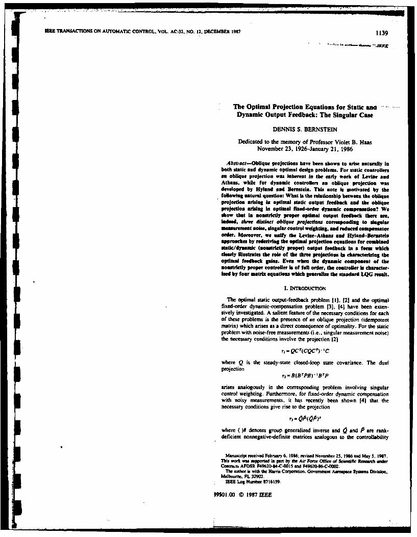
lMEE TRANSACTIONS ON AUTOMATIC CONTROL. VOL. AC-32. NO. 12. DECEMBER IM1 1139

The Optimal Projection Equations for Static ana-Dynamic Output Feedback: The Singular Case

DENNIS S. BERNSTEIN

Dedicated to the memory of Professor Violet B. HaasNovember 23, 1926-January 21, 1986

Abstract-Oblique projections have been shown to arise naturally inboth static and dynamic optimal design problems. For static controllersan oblique projection was Inherent In the early work of Levine andAlbans, while for dynamic controllers tn oblique projection wasdeveloped by Hyland and Bernstein. This note Is motivated by thefollowing natural question: What is the relationship between the obliqueprojection arising in optimal static output feedback and the obliqueprojection arising In optimal fxed-order dynamic compensation? Weshow that In nonstrictdy proper optimal output feedback thene are.indeed, thiec distnct oblique projections corresponding to ingularmeassurement noise, singular control weighting, and reduced compensatororder. Moreover, we unify the Levine-Athans anid Hyland-Berintelnapproaches by rederiving the optimal projection equations for combinedstatic/dynamic (sionstrietly proper) output feedback In a form whichclearly ilustrates the role of t three projections In characterizing theoptimal feedback gains. Even when the dynamic component of theaonstrictly proper controller is of fanil order, the controller is character-Ied by four matrix equations which generalize the standard LQG reslt.

1. INTRODUCTION

The optimal static output-feedback problem [1]. [2) and the optimalfixed-order dynamic-compensation problem [31. [4] have been exten-sively investigated. A salient feature of the necessary conditions for eachof these problems is the presence of an oblique projection (idempotentmatrix) which arises as a direct consequence of optimality. For the staticproblem with noise-free measurements (i.e.. singular measurement noise)the necessary conditions involve the projection 121

7t-QCT(CQCT) 'C

where Q is the steady-state closed-ioop state covariance. The dualprojection

72 =BDOB'PB) -8 7BP

arises analogously in the corresponding problem involving singularcontrol weighting. Furthermore, for fixed-order dynamic compensationwith noisy measurements. it has recently been shown 14) that thenecessary conditions give rise to the projection

where O#denotes group generalized inverse and Q and 1S are rank-deficient nonnegative-dlefinite matrices analogous to the controllability

Manuscript received February 6. 1986; revised November 25. 1986 and May 5. 1967.This woad was suspported in pan by die Air Force Ofie of scientific Research underCantrcti, AFOSR Ft4920-84-C.0Ot5 and F49620-86-C.0002.

The author is with the Haris Corporation. Qovnunent Aerospace systems Division,Melbourne. aL 32902.

MEEE Log Numnber 8716159.

19$01.00 0 1987 IEEE

1140 IEE TRANSACTIONS ON AUTrOMATIC CONTROL, VOL. AC-32, NO. 12. DECEMBER 1987

and observability Oramians of die compensator. To understand the uW~T1 Srelationships among rl, 72, and r3, the contribution of the present noteUi a unifie treatment of the necessary conditions for optimal stalici LNdinamic feedback compensation which clealy lluastrates the role ofthe three projections in characterizing the optimal feedback gains.Even in the full-order case in which T-3 is the identity, the result providesa generalization of the Standard LQG result to nonstrietly proper

* controllers in which case the separation principle does not bold.To clarify the raifications of noise and weighting singularities in

* ~~optimal output feedback. consider the problem of mnmzn

JulimII[xrR~x+uTRauI (0.1) SAI

with plant dynamics CLI

*nAxw+Bu+wa, (1.2) CoD:YATOPC

Y -CX+ wl, (1.3) I

and nionstrctiy proper feedback compensator

4-AxDy. 1.4) out by (1.6) do not appear in Fig. 1. Specifically: 1) nonnoisyu - Cx(1.5)y measurements can be fed back to unweighted controls; 2) dynamic-

As pinte outin []. is init onl ifcompensator outputs can be fed back to unweighted controls; and 3)As pintd ot in[3] J s fiiteonl ifnonnoisy measurements can serve as inputs to the dynamic compensator.

The reaso for considering the more limited configuration shown in Fig.!I0-ty1D,"RIDV1l * -RIDVI (1.6) is that only these paths are explicitly characterized by the necessary

conditions. Hence, for Simplicity we first consider only the scheme ofwhere VI denotes the intensity of wl.. Clearly, when R, and VI ar Fig. 1, and later introduce the remaining permissible paths. Interestingly,nonsingular (1.6) implies D, -0, and hence direct feedthrough is not while these additional gains are not completely determined by the-permitted, i.e., the compensator must be strictly proper. Conversely, to necessary condiitions, they appear to play an important role in governingutilize a static gain D,, either R, or V, must be singular. By writing geometric interrelationships amiong the three projections.singular RI and VI without loss of generality as Two final comments are in order. First, since our results are carried out

-~~ in a multiplicative noise setting, we generalize previous results on state

R. -PjV 0 I(1.7) feedback [ 151-[ 181 and dynamic compensation 191 I]. The motivation0 0 0 j for using a multiplicative white noise model is to represent plant

parameter uncertainties and thereby obtain robust controllers (12]. Also,it follows that the static transmi~ssion between noisy measurements and the derivations of the necessary conditions are straightforward extenisionsweighted controls must be zero (see Fig. 1). of the Lagrange multiplier technique used in 141 and hence have been

The reader will observe that three feedback paths which are not ruled omitted.

1I. NOTATION AND DEFINITIONS

91 Aj"s Q' real numbers, r x s real matrices, Rl" , expectationIJ,,(), ( ~r x r identity, transpose, group generalized inverse ( 13, p. 124]

@, ® Kronecker sum, Kronecker product1. - . T E1111Iasymptotically stable matrix matrix with eigenvalues in open left-half planenonnegative-semisimple matrix semisimple (nondefective) matrix with nonnegative eigenvaluesn, ins. 012, 1,12, n,, p positive integersX- uI, 12 yl, Y2, X, , in11, "12, 11, 12, n,-dimensional vectorsA.,Ai; B,, Bu,; Ci, Cu, n X nimatrices, n x ml matrices, 1, x nrnatrices, i - , pB2. C2 n x mn2 matrix, 12 x IT matrixA,, B,, Cc,, D,,, E, ni, x n,, n, x 11. ml x n,, ml x 12, m2 X I matricesV,(f unit variance white noise, i - 1, - -. pWOOLt), W(t n-dimensional. ,-dimensional white noiseVa. VI intensities of wo, w,; Va a 0, VI > 0Vol n x 11 cross intensity of w0, wlN. R, st and contol weightings; Re 2: 0, R, > 0Rol n x mn1 cross weighting: R0 - R.,R - R~ r 0

A. A, A + DIDC 2 + BifC,, A, + BloD,,C 2 + 53ECl,, i -I . ... p

~~~',~~V Vi' J .~v ,1r R.r.,F~L(BlE,J LV Go J L(3E,)T DC2L 01 R, J DC1J

A BC, A, a,c,]AC ABI,

IEE TRANSACTIONS ON AUTOMATIC CONTROL. VOL. AC-32, NO. 12. DECUM M9 1141

B, V.; + B,(VDe(D2 E,) 1LCrR r+ CRDCc CrR ICc

For arbitrary n X ft Q, P. do A Ti, r2 define: To develop necessary conditions for this; problem. De and Ev must berestricted to the set of second-moment-stabilizing; pins

R15 9 R, + DriPB, Vt la V + t CuQClr. d E A A A Asai-I A j TA A, is~ asyJ+mpl~U u N ioculIybe]

(L AA QCf+ Vol A BT + rAAA~r QCAT++ t**jg jP The requirement (D., Ec) E 6 implies the existence of the steady-stateclosed-loop state covariance Q A urn,.... IKxx(t)Q7J. Futiherime, Q

Als RI+ B'P+ 5)Bj. I,, V,+ C.(g+)Cr and its nonnegative-definite dual P are the unique solutions of theA~ ,X ~PP51 ,PA IfC 1(+)~ modified Lyapurnov equations

AQC~4.VI+~I(Q4)CT, 0AQ+QA'+t A,QAT+ F, (3.7)1-1

&ABrP+R +± Br(P+P)A,, 0-A TP +PA+ t ArPA1 +,N (3.8)

A A A-B,A-'(&,+BP)r-(&+aCr)vICI. An additional technical assumption is that (D,Ejbe confined to the set

A, AAi-iiA~Q~.3rP~i-r(&+ofl%~'Ci, 5 A (D,, Es) E S : CiQCT>0 and R~rPBi>0).

In order to obtain closed-form expressions for the feedback gains we

Aqg. AA-(;±&d-2Qcr) P -' C,Aa. AA-:A'(&,r,-TPr). make the additional assumption here and in Section TV that

A, R.R,, ~i.e., fo~reach i, Bitand Cuame not both nonzero. By optimizing (3.6) with

+ T((1, + r)TA RIA-(&,+Brp)r.. respect to D, and E, and manipulating (3.7) and (3.8), we obtain theIs I tonwing result.

7Teorem 3.)1: Suppose (Do, E) E & * solves the satic output feedbackFla Ja v.-V,P,'(+ic)TT ? 2,(&L+oCrp;,' v; problem. Then there exist n x n nonnegative-definite Q. P such that

+ r:(L+ Qcr) ,' vP p (4,.4.QdrT)rr A- -R ' aQ(CQ ) .(3.10)

Il. STATIC OuTPVT FEEDIAcx E, -- (BPB) -BP.,V~,,(.1

Static Output Feedback Problem and sucht that Q and P satisfy

Given the controlled system Om (A - BjR ~'Pr)+ Q(A - BIR -11 G1.v)T+ V,

14t) (A +± t u(t)A ) +± AB 1 R'6,)QA-,RtPr)

+ B + tu,()t))u1 t) + IU2(t) +wg(t), (3.1) -0. V - ~I qr+ ., VI rr (3.12)

(c+±~~I Is)i)Q+w) (3.2

Y20t) -Czx(t) (3.3) 1

where t6 10, ap), determine D, and E, such that the static output -j'R -tt,+,rd (3.03)feedback'law

aa1()-D~,Q).(3.4) where

u2)Ey()(3.5) 'r A QC( 1QC)- 1, (3.t4)

miiie h etma.c criterio n1 A B(BrP~a)-'BrP. (.5

1 la tim IIxQ)?R~x(f),2xQ)TRolui(,)+ulQ)Ru(). (3.6) Remark 3.: Severa special cams can be recovered formally from

a-- Theorem 3. 1. For example, when the COauol weighting is foangular

1142 IEE TRANSACTIONS ON AUTOMAT1C CONTROL VOL. AC-32, NO. 12, DECEMBER M

and the measurement noise is zero. i.e., when ul and Yj are absent, delete P, Q. P such that(3.11) and set r2-0. Deleting also the multiplicative noise terms yieldsthe usual static output feedback result [1), 12]. A,=r(A -BtA ,, )Gl, (4.10)

IV. DYNAMIC OUTPUT FEEDBACK B,-r(ri .L - r t

o p

We now expand the formulation of the static problem to include apurely dynamic (strictly proper) dynamic compensator. c,- - A B SP,)Gr, (4.12)

Dynamic Output Feedback Problem A- -A -'( +Brp) r(C=r)- ,(

Given (3.4)-(3.3), determine A, B, C,, D,, E. such that the static anddynamic output feedback law E-- (BrPB,)- 'BTP(4, + QCr) P' (4.14)

te(t)=A,x,(t)+By,(t), (4.1) where 71 and "2 are given by (3.14) and (3.15), G, r satisfy (4.Sa),

uit)= C~vx,)+DY 2 ), (4.2) (4.8b), and such that, with 73 given by (4.9), Q, P, 0, and 5 satisfy i

u2(t)= Ey(t) (4.3) 0,,,,AQ+QAT+ 7+ JAQA T+ (A,-B,,-A B,', Br

minimizes the performance criterion (3.6).We restrict our attention to second-moment-stabilizing controllers • - B,, -' [( ,rt £ - B T

Is iIs( -

,)A A., ,DE,:A$A+ A , is•24L,2~ r+3L7 ,,7Q, p,, (,.,,-r,-,, r Trr

asymptotically stable and (A,, B,, C,) is minimalj. (4.15)

which implies the existence of 0 A lim,_, Li TI2(t)T , where 9(t) o( 4X)T, 7,Q) 7 r . Furthermore, a and its dual P are the unique solutions ArP+PA +A0 + t IAfPA4+(A - [?2L ridCr] P -'C.,) Iof the modified Lyapunov equations -

0A +QA' +' AQA + V. (4.4) " 1 Br" ,)] (( ," .-BrPv ) I• ,,-Br[ ,)+,rr(,T., -Ba[",,),,e '(&,,,, -BAl,.),,.

0=ATP +PA+j A -AT + 4.5) (.64-I U

Partitioning 0=Ah+ CA r + & - " Is) P '('z, &,- ? CD r

wher. and = [ , j:] * [P, P' ] -.r, (, .- .r)-(7302.. -7 0cT 31. (4.17) 3P1 P12

where Q12 and P,2 are n x n,, we also require OA9A+8AA,.(',r,. -R P),-( ',, -BIs )Z' ai {(A_ B,, C,. D_, E,) E 0: : C:(Q - Q,zQ -'Q[)C7'>0 -Tr ( , _rrrj ,(,, _[r)].(4.18) .

and BT(PI-PI2p;'pr)B2 >O}" rank 0-rank P=-rank C15=n,. (4.19) 3Optimizing (3.6) over ZD, introducing new variables Remark 4.1: Setting r = r= 0, D, =0, E, = 0 yields the results of U

Q i Q,-Q,2Q;'Q',r P a P,-P, PZ'P2. (4.6) [4], [11].Remark 4.2: Suppose.n,=n so that 73=1,. Then the resulting full-

S-Q,,QQ;Q , PjC. p,1 p;'pr, (4.7) order nonstrictly proper controller is characterized by four matrix Iequations which generalize the standard LQG result. In this case theand manipulating (4.4) and (4.5). we obtain the dynamic extension of separation principle is no longer valid.Theorem 3. 1. The following lemma is required for the statement of theresult. V. ADDITIONAL FEEDBACK PATHS

Lemma 4. ): Suppose n X n" . J are nonnegative definite. Then iOPis nonnegative semisimple. If, in addition, rank 10= ni, then there exist We now introduce the feedback paths not shown in Fig. I. For the staticn, x n G, r and n, x nc invertible M such that problem replace (3.5) by

O ' P=GrTA , rGr=i.,. (4.ga,b) u:(t)=Ey,(t)+K,y2 (t). (5.1) 3Proof. The result follows from [14, Theorem 6.2.51. Optimizing with respect to K, yields the additional condition

Since QP is semisimple it has a group inverse (Q)' = GrM r and 0- C QPBj (5.2), 4 05(oP)'-Gr (4.9) which implies

is an oblique projection. 0-rr,. (5.3)Theorem 4.1: Suppose (A e, B,, C,, D,, E) 6 1) solves the dynamic 3

output feedback problem. Then there exist ft x n nonnegative-definite Q, This geometric condition holds when K, is optimally chosen. Although K

IEEE TRANSACTIONS ON AUTOMATIC CONTROL, VOL. AC-32. NO. 12. DECEMBER 1987 1143

ia notl given explicitly, zt does play a role in the necessary conditions since 0 =A j2+ ORT + 72, 4L P.-'QA isreptaced by A + BIX1 C2.

For the dynamic problem replace (4. 1) and (4.3) by T ?2&C'TT-G KCQ.QKC) (.)

2 ,() -E .YiQ) + K yxQ) + K~y2 (). (5.) O = r) P +P ,, (! 5Trr -T r ~ 2 2 .P X 52 , (.

Optimizing with respect to K,, K2, K3 yieldswhere

0=C =(QPO+ 2 ), (5.b) AS=A+B,IC2 -GKC2, A,=A+B2K ,+B2K~r,

0=aPB,. 4 A0+B2 K.C2-G TX,, A, A A,+B 2K1 ,+B 2x~r.

S= C, QP. (5.6c)V1. DIRECTIONS FOR FURTHER REsEARCH

which implyMore general solutions can be obtained by incorporating singular

0 ri~.(5.7a) estimation techniques [15] where noise-free measurements are repeatedly

0 - 773, (.7b) differentiated to enlarge the class of available outputs.

0 37.(5.7c) ACKNOWLEDGMENTThe author wishes to thank D. C. Hyland for numerous helpful

Note that (5.7b) and (5.7c) imply discussions.

0-7T71-(5.8) REFERENCESUsin (S7b) (57c) ~ ~ P =A'~(se [4), 4. I)-(. I) bco III1 W. S. Levine and M. Admits, "On the determination or the optimal constant

Usin (57b) (5.7c) Q1 riQ, fit (se (4), 4.1)-(4 18 beome output feedback gains for linear multivaniable systems," IEEE Trans. A utonte.Con,,., vol. AC-IS, pp. 44-48, 1970.

A,- (A 8, -% A, P-C,+BK . - C~r 121 J. Medanic. -On stabilization and optimization by output feedback.- Proc. 12th1. Is)GT +rBK.,Asilomaur Con!. Circ.. Syst. Comp., Pacific Grove. CA. Nov. 1978. pp. 412-

416.(5.9) 131 S. Bauhakur and C. H. Knapp, "Optimal constant controllera for stochastic

linear systems." IEEE Trants. Automat. Conitr.. vol. AC.20. pp. 6"4-W6.1975.

B, r..41 Is(5.10) 14] D. C. Hyland and D. S. Bernstein, "The optimal projection equations for fixed-order dynamic compensation, " IEEE Trans. Austomnat. Contr., vol. AC-29. pp.1034-1037. 1984.

C .= ~I~t 1 G T. (5.11) [51 W. M. Wonhamn. "Optimal stationary control of a linear systemn with state-dependent noise." SIAM J. Contr., vol. S, pp. 486-300. 1967.

161 D. Kleinman. "Optimal stationary control of linear systems with control-D = -. 4 J51QCT(CQCT)-i, (5.12) dependent noise.' IEEE ras. Automat. Con:,.. vol. AC-14. pp 673-677,

Is 2 21969.[71 P. McLane, "Optimal stochastic control of' linear systems with state and control-

E,= (8fB)-IBr( (5.13) dependen disturbances." IEEE Trans. Automat.. Contr.. vol. AC- 16. pp. 79.3-2 Is 798. 1971.

181 J. Bistnut. "Linear-quadratic optimal stochastic control with random coeff'i-I, cients." SIAM J. Contr., vol. 14. pp. 419-444f. 1976.

0 =A4 Q + QA T+ P0+ IAQAr+ (A, - A, it., (91 0. N. Mil 'stein. "Design of stabilizing controller with incomplete state dat forlinear stochastic system with multiplicative noise." Automat. Remote Contr..vol. 43, pp. 653-659, 1982.

A A ' A A 'T T(101 Y. A. Phillis. 'Controller dcsign of systems with multiplicative noi',c ' IEEEIs 24 TransAutomat. Cont.. vol. AC-30. pp. 1017-1019. 1985.

fill D. S. Bernstein and D. C. Hyland. "The optimal projection/maximum entropy-1 r r 5.4 approach to designing low-ordcr. robust controllers for flexible stmrure .- in

Lv "zQ Q~,' 72, 73, ( Proc. 24Mh IEEE Conf. Decision Contr.. Fort Lauderdale. FL. Dec 1985. pp.745-752.

P 1121 D. S. Bernstein and S. W. Greeley, "Robust controller synthesis using theo=Ap~p2+ 0.,~ 1rPA+(A+r2 l~C,,)r maximum entropy design equation%," IEEE Trans. Automat. Contr., vol. AC-o I A ,- rA A+T 31. pp. 362-364, 1986.

[131 S. L. Campbell and C. 'D. Meyer. Jr.. Generalized Inverses of Linear

~1. 1141Transformations. London: Pitman. 1979.- AN - A 9 C01- T ,Tg'&,,, 141C. R. Rao and S. K. Mitts. Generalized Inverse of Matrices and Its

Applications. New York: Wiley. 1971.+?~~ ~~~-~? i~(5.5) liSI V. B. Haas. "Reduced order state estimation for linear systems with exact

me+rmns uoa/a vol. 20. pp. 223-229. 1984.

I

1 1989 ACC

II'I

A Riccati Equation ApproachI to theSingular LQG Problem

3 (ABSTRACT)

I

I by

I

Yoram Halevi Wassim M. Haddad Dennis S. BernsteinFaculty of Mech. Engineering Department of Mechanical Government Aerospace

Institute of Technology and Aerospace Engineering Systems DivisionHaifa 32000 Florida Institute of Technology Harris Corporation,

Israel Melbourne, FL 32901 Melbourne, FL 32902

I

II3'

I , m

II II

1. Introduction

The singular LQG control problem has been of considerable interest for almost two decades 3(11-15]). Such problems arise when some of the measurements are noise free or when some of the

control signals are unweighted. This will be the case, for example, if the sensor noise is colored or

if actuator dynamics are included. Augmentation of the plant dynamics by means of noise filters

or actuator dynamics thus leads directly to the singular problem formulation. 1Most of the literature on the singular LQG problem is based upon limiting procedures in which

suitable weighting matrices and noise intensities approach zero. These results demonstrate the

types of behavior which can arise in the limiting solution including impulsive controls and singular

arcs.

The available literature is concerned, of course, with determining the optimal limiting (i.e., 3singular) control. In practical applications, however, it is often of interest to determine the optimal

controller within a prespecified class of controllers. In particular, we consider the singular LQG

problem in which the controller is preconstrained to possess a fixed dynamic feedback structure.

One benefit of this approach is that the fixed structure constraint eliminates the possibility of

impulsive controls and other complex behavior.

Preliminary results for the singular LQG problem were obtained in [15] using the fixed struc- 3ture approach. For generality, the problem considered in [15] permits the design of fixed-order,

i.e., reduced-order, dynamic compensators. As in [18], the solution is given by a system of coupled

algebraic Riccati and Lyapunov equations whose solutions (denoted by Q, P, (, P) are used to ex-

plicitly characterize the optimal feedback gains. The coupling is due to a pair of oblique projections3

(i.e., idempotent matrices) which arise as a direct consequence of the fixed structure constraint.

Theorder-reduction projection r definedby

S,415m

where ()# denotes group generalized inverse, appeared originally in [16], while the static projection 3v given by ° c(cqc)-lc, 311 A QC T CQC T )-C

is familiar from least squares analysis.

The results of [15] are incomplete, however, in that the gains associated with certain feedback 1paths were not given explicitly. For the corresponding singular estimation problem ([17]) this de-

11

-- . . , i , I I I I I I I II

III

I fect was remedied in [181 where all feedback gains were explicitly characterized. In addition, the

solution obtained in [18] was shown to agree completely with results obtained using standard lim-

iting methods when the (unconstrained) optimal singular estimator does not possess differentiators

([19]). The results of [18] thus provide an alternative approach to the singular estimation problem

considered in [20,21,22] and the numerous references therein.

3 The contribution of the present paper is thus to complete the development of [15] by incorpo-

rating the methods used in [18]. Accordingly, we derive a coupled system of modified Riccati and

Lyapunov equations which explicitly characterize the feedback gains of the fixed-structure singular

LQG controller. For generality we consider partial or total singularity in both the control weight-

ing and measurement noise intensity matrices, and we allow the dynamic compensator to be of

arbitrary dimension less than or equal to the number of plant states minus the number of noise-

free measurements. In the special case in which the order of the dynamic compensator is equal to

the number of plant states minus the number of noise-free measurements (i.e., the quasi full-order

case), then we show that the optimal solution decomposes (separates) into a reduced-order observer

followed by state feedback.

3An additional benefit of our approach is the ability to impose an upper bound on the number

of differentiators to be included in the feedback controller. That is, while certain measurement3 signals may be noise free and hence differentiable, it may be undesirable in practice to implement

more than one level of differentiation or, perhaps any differentiation at all. Furthermore, as in [1813 we demonstrate connections with earlier results by showing that the fixed structure solution agrees

with the standard limiting solution when the latter possesses the same number of differentiators as3 are included in the prespecified controller structure.

To illustrate the solution we consider a numerical example of fourth order with two noise-3 free measurements and one noisy measurement. (Numerical results for the singular control case

are immediate from duality). By solving the coupled systems of modified Riccati and Lyapunov3 equations by means of a homotopy algorithm ([23]), we obtain the quasi full-order solution (second-

order controller) as well as an optimal first-order controller.

1 23

References I1. B. Friedland, "Limiting Forms of Optimum Stochastic Linear Regulators," Trans. ASME J.

Dyn. Sys. Meas. Contr., Vol. 93, pp. 134-141, 1971.

2. Y.-C. Ho, "Linear Stochastic Singular Control Problems," J. Optim. Thy. Appl., Vol. 9, pp.24-31, 1972.

3. M. F. Hutton, "Solutions of the Singular Stochastic Regulator Problems," Trans. ASME J.Dyn. Sys. Meas. Contr., Vol. 95, pp. 414-417, 1973.

4. H. G. Kwatny, "Minimal Order Observers and Certain Singular Problems of Optimal Estima-tion and Control," IEEE Trans. Autom. Contr., Vol. AC-19, pp. 274-276, 1974.

5. R. E. O'Malley, Jr., and A. Jameson, "Singular Perturbations and Singular Arcs - Part I,"IEEE Trans. Autom. Contr., Vol. AC-20, pp. 218-226, 1975. U

6. R. E. O'Malley, Jr., and A. Jameson, "Singular Perturbations and Singular Arcs - Part II,"IEEE Trans. Autom. Contr., Vol. AC-22, pp. 328-337, 1977. I

7. B. A. Francis and K. Glover, "Bounded Peaking in the Optimal Linear Regulator With CheapControl," IEEE Trans. Autom. Contr., Vol. AC-23, pp. 608-617, 1978.

8. B. A. Francis, "The Optimal Linear-Quadratic Time- Invariant Regulator with Cheap Control,"IEEE Trans. Autom. Contr., Vol. AC-24, pp. 616-621, 1979. 3

9. V. Dragan and A. Halanay, "Cheap Control and Singularly Perturbed Matrix Riccati Differ-ential Equations," Rev. Roum. Math. Purea et. Appl., Vol. 26, pp. 21-40, 1981.

10. V. B. Haas, "The Singular Steady State Linear Regulator," SIAM J. Contr. Optim., Vol. 20, Ipp. 247-257, 1982.

11. J. O'Reilly, "Partial Cheap Control of the Time- Invariant Regulator," Int. J. Contr., Vol. 37, Ipp. 909-927, 1983.

12. P. Sannuti, "Direct Singular Perturbation Analysis of High-Gain and Cheap Control Problems,"Automatica, Vol. 19, pp. 41-51, 1983. I

13. M. L. J. Hautus and L. M. Silverman, "System Structure and Singular Control," Lin. Aig.Appl., Vol. 50, pp. 369-402, 1983. I

14. Y. Halevi and Z. J. Palmor, "Extended Limiting Forms of Optimum Observers and LQGRegulators," Vol. 43, pp. 193-212, 1986. 3

15. D. S. Bernstein, "The Optimal Projection for Static and Dynamic Output Feedback: TheSingular Case," IEEE Trans. Autom. Contr., Vol. AC-32, pp. 1139-1143, 1987.

16. D. C. Hyland and D. S. Bernstein, "The Optimal Projection Equations for Fixed-Order Dy-namic Compensation," IEEE Trans. Arutom. Contr., Vol. AC-29, pp. 1C34-1037, 1984.

17. W. M. Haddad and D. S. Bernstein, "The Optimal Projection Equations for Reduced Order UState Estimation: The Singular Measurement Noise Case," IEEE Trans. Autom. Contr., Vol.AC-32, pp. 1135-1139, 1987. 1

I

18. Y. Halevi, "The Optimal Reduced Order Estimator for Systems with Singular MeasurementNoise," IEEE Trans. Autom. Contr., Vol. 34, 1989.

19. Y. Halevi, "Limiting Forms of Optimal Observers" Int. J. Contr., Vol. 47, pp. 209-216, 1988.

20. A. E. Bryson and D. E. Johansen, "Linear Filtering for Time Varying Systems Using Mea-surements Containing Colored Noise," IEEE Trans. Autom. Contr., Vol. AC-10, pp. 4-10,1965.

21. J. M. Schumacher, "A Geometric Approach to the Singular Filtering Problem," IEEE Trans.Autom. Contr., AC-30, pp. 773-776, 1985.

22. E. Soroka and U. Shaked, "Direct Solution to the General Reduced Order Stochastic Observa-U tion Problem," Int. J. Contr., Vol. 45, pp. 713-728, 1987.

23. S. Richter, "A Homotopy Algorithm for Solving the Optimal Projection Equations for Fixed-Order Dynamic Compensation: Existence, Convergence, and Global Optimality," Proc. Amer.Contr. Conf., pp. 1527-1531, Minneapolis, MN, June 1987.

II'II

IIIIIII.. . iiIIIIIIiII

APPENDIX F: Stochastic Modeling

I3. D. S. Bernstein and D. C. Hyland, 0'lbs Optiual Projectio/MaidnuEntrcpy Approach to Designing Low-Order, Prbuist Controllers forFlexible Structures," Proc. 24th IEE af. Dec. Cwtr., pp. 745-752,Fort Latderdale, FL, December 1985.I 36. D. S. Berntein, L. D. Davis, S. W. Greeley arid D. C. Hylandi,"Niuerical Solution of the Optimal Proj ectictVaxinui Entrcpy DesignEquations for Ltaw-Orde, Rust Qmitroller Design," Proc. 24th IE

Cn. Dec. Cotr., pp. 1795-1798, Fort Lauderdale, FL, Decemb~er 1985.

1104. D. S. Bernstein and D. C. Hyland, "Cptinal Projection Equations forReduoad-Order Modelling, Esiainand Control of Linear Systemswith Multiplicative Itite Noise," J. (tm. Thy. h=x~., Vol. 58, pp.

387-409, 1988.

39. D. S. Bernstein and S.* W. Greeley, IT~bst Cantroller Synthiesis Usingthe ?bximn Entropy Design Equatioins," IEE frans. Autom. Qitr.,Vol. AC-31, pp. 362-364, 1986.

I 77. D. S. Bernste-in, "Robst Static and! Dynamnic Output-FeedbacStabilization: Deem nisi dsi Stochastic Perspectives,"Irans Auxtam. Ccsytx., Vol. AC-32, pp. 1076-1084, 1987.

I

iI

I

HTA3- 10:30THE OPTIMAL PROJECTION/MAXIMUM ENTROPY APPROACH

TO DESIGNING LOW-ORDER, ROBUST CONTROLLERSFOR FLEXIBLE STRUCTURES

Dennis S. Bernstein and David C. Hyland m

Harris CorporationControls Analysis and Synthesis Group I

Melbourne, Florida 32902 IAbstract. The Optimal Projection/Maximum Entropy with regard to the latter item, it should be

- stressed that one of the major problems inapproach to designing low-order controllers for designing high-performance control systems ishigh-order systems with parameter uncertainties that of robustness, i.e., the ability of the

controller to toTerate errors in the plant modelis reviewed. upon which its design is predicated. Maximum

by incorporating into the dynamic model a repre-

parameters by means of Stratonovich sentation of ignorance (i.e., uncertainty)multiplicative white noise is motivated by means regarding physical parameters. Roughly speaking,

the idea behind the approach is to use a probabi-of the Maximum Entropy Principle of Jaynes and listic representation of each imperfectly knownstatistical analysis of modal systems. The main plant parameter so that the quadratically optimal

control system designed under this probabilisticresult, the optimal projection equations for model is automatically desensitized to actual

fixed-order dynamic compensation in the presence parameter variations when the control sys%-is implemented. The overall control-design

of state-, control- and measurement-dependent procedure thus avoids laborious trial and error

noise, represents a fundamental generalization of post-design "tweaking."

classical LOG theory. 2. Motivation

1. Overview The inherent time- and frequency-domain dualityin representing linear dynamic systems (i.e.,

Optimal Projection/Maximum Entropy Stochastic state space versus transfer functions) providesModelling and Reduced-Order Design Synthesis control-system designers with complementaryis a rigorous new approach to designing robust, methodologies for assessing tradeoffs betweenimplementable feedback controllers. Inspired performance objectives and the design constraintsby Statistical Energy Analysis [1], a branch of of sensor resolution, actuation levels, plant Idynamic modal analysis developed for analyzing modelling accuracy and controller complexity. Inacoustic vibrations, its present stage of spite of the ability of LOG to optimally quantifydevelopment [2-22), embodies a mathematically performance/sensor-resolution and performance/rigorous, fundamental generalization of classical actuation-level tradeoffs in a state-spacesteady-state Kalman filter and linear-quadratic- setting, its enormous sensitivity to plantGaussian (LQG) optimal control theory. Although modelling errors has forced practitioners to seekLQG theory is an effective tool for optimally generalizations of classical frequency domainquantifying performance/sensor-resolution and methods. In numerous practical situations,performance/actuation-level tradeoffs, it suffers however, input/output techniques possess funda-from two fundamental defects which' severely limit mental limitations. For example, representingits usefulness in practice. modelling uncertainty in a frequency-domain plant

model G(s) by means of1. Whereas the dimension of an LQG

controller must equal that of the controlled G(s) +&G(s),

plant, optimal projection design characterizesthe quadratically optimal controller of fixed where AG remains in a normed neighborhood of G,dimension less than that of the plant in is essentially a black-box (nonparametric)accordance--h implementation constraints (e.g., approach: By failing to exploit physical lawsreliability, complexity or real-time computing (such as conservation of energy), systemscapability), represented by G + AG may actually be physically

impossible, resulting in unwarranted design2. Whereas LQG presumes exact knowledge of conservatism at the expense of system

each and every parameter appearing in the state- performance. Hence, when some knowledge of

space plant description, maximum entropy Internal mechanisms is availablb (i.e.. the

modelling provides a stochastic plant model which "grey-box" situation), state-space representa-admits ignorance with regard to parameter values tions may provide greater modelling fidelity.in accordance with unavoidable plant model ling These observations are motivated by the problemieaord e wof controlling vibration in flexible structures

errors.745 CH224-9/85f000-743 $1 .(1A C 1983 IEEE m

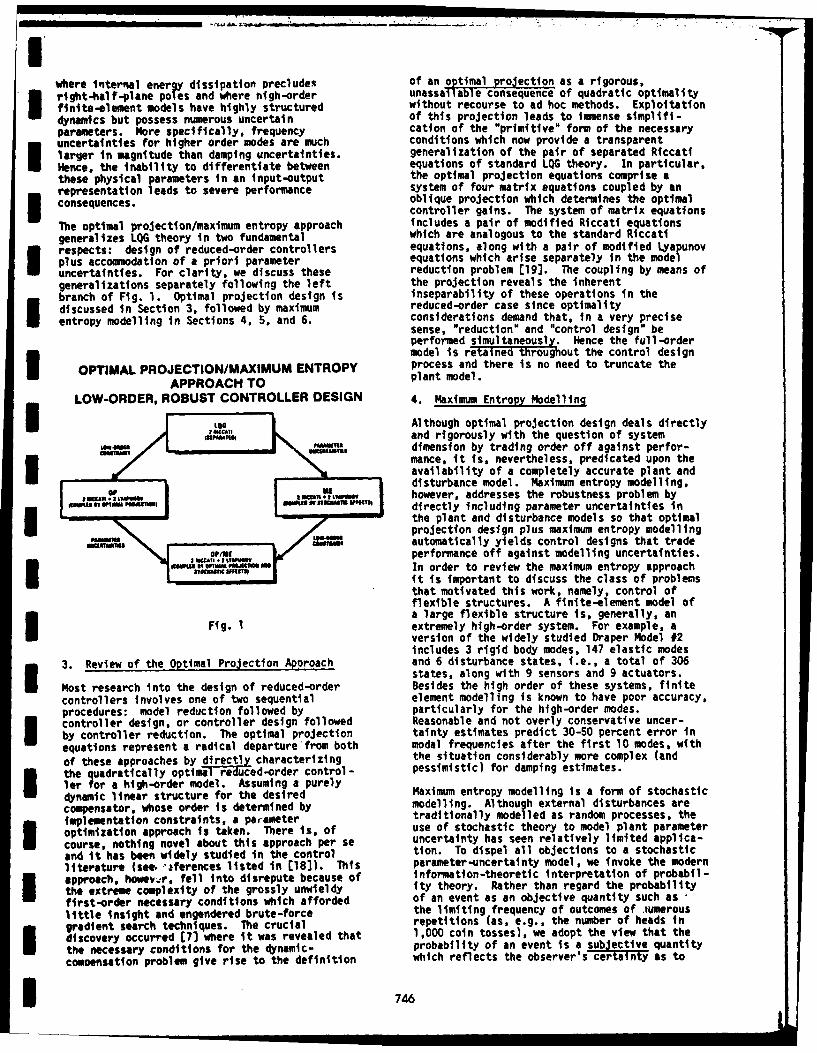
Iwhere internal energy dissipation precludeS of an optimal projection as a rigorous,

* right-half-plane poles and where nigh-order unassailable consequence of quadratic optimalityfinite-element models have highly structured without recourse to ad hoc methods. Exploitationdynamics but possess numerous uncertain of this projection leads to immense simplifi-parameters. More specifically, frequency cation of the "primitive" form of the necessaryuncertainties for higher order modes are much conditions which now provide a transparentlarger in magnitude than damping uncertainties, generalization of the pair of separated RiccatiHence, the inability to differentiate between equations of standard LQG theory. In particular.these physical parameters in an input-output the optimal projection equations comprise arepresentation leads to severe performance system of four matrix equations coupled by an

* consequences. oblique projection which determines the optimalcontroller gains. The system of matrix equations

The optimal projection/maximum entropy approach includes a pair of modified Riccati equationsgeneralizes LQG theory in two fundamental which are analogous to the standard Riccatirespects: design of reduced-order controllers equations, along with a pair of modified Lyapunovplus accommodation of a priori parameter equations which arise separately in the modeluncertainties. For clarity, we discuss these reduction problem [19]. The coupling by means ofgeneralizations separately following the left the projection reveals the inherentbranch of Fig. 1. Optimal projection design is inseparability of these operations in the

* discussed in Section 3, followed by maximum reduced-order case since optimality

entropy modelling in Sections 4, 5, and 6. considerations demand that, in a very precisesense, "reduction" and "control design" beperformed simultaneously. Hence the full-ordermodel is retained throughout the control design

OPTIMAL PROJECTION/MAXIMUM ENTROPY process and there is no need to truncate the

APPROACH TO plant model.

LOW-ORDER, ROBUST CONTROLLER DESIGN 4. Maximum Entropy Modelling

LAlthough optimal projection design deals directlyand rigorously with the question of system

PAI, R dimension by trading order off against perfor-

mance, it is, nevertheless, predicated upon theI availability of a completely accurate plant anddisturbance model. Maximum entropy modelling,

I Mhowever, addresses the robustness problem byON%" ma-nu, u,, directly including parameter uncertainties in

the plant and disturbance models so that optimalprojection design plus maximum entropy modelling

CM "automatically yields control designs that tradeperformance off against modelling uncertainties.In order to review the maximum entropy approachit is important to discuss the class of problemsthat motivated this work, namely, control offlexible structures. A finite-element model ofa large flexible structure is, generally, an

Fig. 1 extremely high-order system. For example, aversion of the widely studied Draper Model #2includes 3 rigid body modes, 147 elastic modes

3. Review of the Optimal Projection Approach and 6 disturbance states, i.e., a total of 306states, along with 9 sensors and 9 actuators.

Most research into the design of reduced-order Besides the high order of these systems, finitecontrollers involves one of two sequential element modelling is known to have poor accuracy,procedures: model reduction followed by particularly for the high-order modes.controller design, or controller design followed Reasonable and not overly conservative uncer-by controller reduction. The optimal projection tainty estimates predict 30-50 percent error in

equations represent a radical departure from both modal frequencies after the first 10 modes, with

of these approaches by diretl characterizing the situation considerably more complex (and

* the quadratically optima-e uced-order control- pessimistic) for damping estimates.

ler lor a high-order model. Assuming a purely Maximum entropy modelling is a form of stochasticdynamic linear structure for the desiredcompensator, whose order Is determined by modelling. Although external disturbances are

I mplementation constraints, a parameter traditionally modelled as random processes, theoptimization approach is taken. There is, of use of stochastic theory to model plant parametercourse, nothing novel about this approach per se uncertainty has seen relatively limited applica-

and it has been widely studied in the control tion. To dispel all objections to a stochastic

literature (see. ferences listed in [18]). This parameter-uncertainty model, we invoke the modern

I approach, howev,:r, fell into disrepute because of information-theoretic interpretation of probabil-

the extreme complexity of the grossly unwieldy ity theory. Rather than regard the probability

first-order necessary conditions which afforded of an event as an objective quantity such as *

little insight and engendered brute-force the limiting frequency of outcomes of iumerous

m gradient search techniques. The crucial repetitions (as, e.g., the number of heads in

discovery occurred E7] where it was revealed that 1,000 coin tosses), we adopt the view that the

the necessary conditions for the dynamic- probability of an event is a subjective quantity

comoensation problem give rise to the definition which reflects the observer's any as to

*'I746

I I .. II

whether a particular event will or will not To see why (5.1) is a minimum information modeloccur. This quantity is nothing more than a of parameter yncertainty, note that when themeasure of the information (including, e.g., pattern /11/ 11 of an uncertain parameterall theoretical analysis and empirical data) iavailable to the observer. In this sense the 1s known, all available data (theoretical andvalidity of a stochastic model of a flexible empirical) can be used to determine a suitablestructure, for example, does not rely upon the value for the magnitude 1 A11 to rflect theexistence of a fleet of such objects (substitute corresponding level of uncertainty. Clearly thePensemble" for "fleet" in the classical termi- collection of magnitudes constitutes the minimumnology) but rather resides in the interpretation data set needed to render (5.1) well defined.that it expresses the engineer's certainty or For the harmonic oscillator with uncertainuncertainty regarding the values of physical natural frequency, the uncertainty magnitude isparameters such as stiffnesses of structural given by the reciprocal of the decorrelation timecomponents. This view of probability theory has (Fig. 2). Note that the uncertainty represen-its roots in Shannon's information theory but was tation (5.1) is a minimum information model infirst articulated unambiguously by Jaynes [23-26]. the sense that it eschews detailed descriptions

of joint probability statistics of unknown IThe preeminent problem in modelling the real oarameters.world is thus the following: Given limited

(incomplete) a priori data, how does one Mconstruct a well-defined (complete) probability MINIMUM-INFORMATION MODELLINGmodel which is consistent with the available data DECORRELATION TIMEbut which avoids inventing data which does notexist? To this end we Invoke Jaynes' Maximm Ii]

n-tropy Principle: First, define a measure ofignorance in terms of the information-theoretic * Ientropy, and then determine the probability T A .im .sdistribution which maximizes this measure subject F1.. • PAMUM DIUTRg OF .NFICTING VOCIATMS.to agreement with the available data. Thereasoning behind this principle is that the Fal NRS EFor.. I . FnU XPOU IN .. fl

probability distribution which maximizes thea priori ignorance must be the least presumptive(i.e., least likely--nvent data) on theaverage since the corresponding amount of e ' 1a posteriori learned information (should alluncertainty suddenly disappear) would necessarily AVMO FAI RESPO.SEbe maximized. If, for some probability distribu- T a "AMPING" T-I COUST-V-tion, the a priori ignorance and hence the r A sTAvwC UNCENATY NMUSlIa posteriori learning were less than their poten-tially maximum value, then BTi distribution must Tbe based upon invented and hence generally incor-rect data. The Maximum Entropy Principle isclearly desirable for control-system design where Ithe introduction of false data is to be assidu- Fig. 2ously avoided.

5. Minimum-Information Modelling ofParameter Uncertainties To eliminate the white noise formalism, the model

(5.1) is usually rigorized by the Ito differen-For dynamical-system modelling it was first shown tial equationby yland [2] that for structural systems theminimum information linear stochastic dynamic P (model induced by the Maximum Entropy Principle of d-t - (Adt + 2 dVtlAI)it t+ cat, (S.2)Jaynes is a Stratonovich multiplicative white i-1noise model. In the present paper we adopt thismodel and explore its ramifications for general where dvit and dwt are Brownian motions,systems. The basic model is given by i.e., Wiener processes. Although such models

were studied extensively for control design, thisA. approach fell into disrepute with the publication

(t) (-+ v(t))x(t) +;(t), (5.1) of [27, 28) where it was shown for discrete-timeI systems that sufficiently high uncertainty levels

(i.e., magnitudes I ItII above a "threshold")where Z(t) R , A e ? ;(t) is zero- lead to the nonexistence of a steady-state

mean Gaussian white disturbance noise with solution. Although it was purported that thisnon-negative-definite intensity V. and vt(t) phenomenon" was an "obviousm consequence of

high uncertainty levels, these conclusionsare zero-ean, unit-intensity Gaussian white failed to take into account (possibly because ofnoise processes which are mutually uncorrelated the discrete-time setting) the subtleand uncorrelated with i(t). The multiplicative relationship between the ordinary differentialwhite noise model (5.1) can be regarded as a equation (5.1) and the stochastic differentialparameter uncertainty model where each vi(t) equation (5.2). Indeed, it was shown in [29]

corresponds to a single uncertain parameer whose that if a stochastic differential equation Iscottrnsnd moanitde arerivn by e regarded as the limit of a sequence ofPatAern approximating ordinary differential equationsand IIX,1'. respectively, then (5.2) is not the cnrrect version of (5.11.

747

Instead, the ordinary differential equation (5.1) to address the following question: Now do theI with multiplicative white noise corresponds to solutions of the stochastic Lyapunov equationsthe corrected Ito differential equation (5.7) and (5.8) differ from each other and from

the "deterministic" Lyapunov equation&t. (W sdt + EP dv,.t,)it + d t, (S.3) z r+V 59* 4' dvti • (t) '(t) + '(t)TT + V, (59)

where particularly in the presence of high uncertainty

levels? The answer to this question of course* + 1 P . depends upon the stochastic modification terms

As + I (S.4) which for the naive model are given by

which differs from the "naive" equation (5.2) M!IL(t)] # E,((t)Xr (5.10)by a systematic drift term. The form of (5.3) 1ll iwas corroborated completely independently byStratonovich E30), whose results actuallyappeared in the Russian literature prior to1965. His approach is based upon an alternative and for the corrected model bydefinition of the stochastic integral whichdiffers from the Ito definition by a mathematicaltechnicality. I -2 :-.T.

!!5 [Q(t)]= _r 1 (FAZ(t) + Q(t)Ai+ ib()AP). (5.11)In spite of the glaring technicality of the t-1

* Stratonovich correction, almost all researchon the estimation and control of such systems Consider a system consisting of apair of lightlyfailed to perceive its physical significance. damped modes so that

* Specifically, the Stratonovich correction -~neutralizes the "threshold uncertainty 01principle": For systems which are inherently 212nl 0stable under particular parameter variations(e.g., structures with uncertain stiffnessmatrices), the Stratonovich formulation correctly 0predicts unconditional second-moment stability incontrast to the Ito formulation within which astringent uncertainty threshold is encountered. Where " Ci w . and to representWe shall now proceed to demonstrate this fact by frequency uncertainties letmeans of a compelling example relevant to themodeling and control of flexible structures, inparticular, and hyperbolic systems, in general.

are of interest and are evaluated according to 10 0 0j

J Iim Ex(t)TRj(t) -Ir tr (t)R, (5.5) 0 0 0whtrdv the 0 0-0

whee ER~l~f nd hesecond moment of the0 0 01state is A2 "y2 0 0 ,

Qlt) E#[(t(t)T]. (5.6)

where for simplicity we have ignored the effects

The obvious fact cannot be overemphasized that of frequency uncertainties on the effective decay

the primary state statistic of design interest in rate 17. The magnitudes of the uncertaintieslinear-quadratic optimization is the state are scaled by means of V1 and -f,. For thiscovariance (5.6). From Ito calculus it follows example the Ito stochastic modificationthat 4(t) is given for the naive model (5.2) by aMIl (t)lhe to soc m

Imlt+t)Jhas the form

A(t + -T (57 2'-T+1.1 VI' 22(t) -V 1 2 (t) 00

and for the corrected model (5.3) by 2 ~ ~ 1 t

I(t~ ~ot + (t)r- + f q ~t" -T + V. (5-8) 0 0 Y!,-,(t) -"Q t

Each of these "stochastic" Lyapunov differential 0 0 -V34(t) 3 3 (t}

equations, which govern the evolution of thesecond moment, should be regarded as n(n+l)/2ordinary differential equations. Hence we wish

l 748

iIAlthough the off-diagonal terms have a becomes increasingly diagonally dominant withstabilizing effect, its clear that the diagonal increasing frequency and thus assumes theelements destabilize the state variances. Hence, qualitative form given in Fig. 3. The benefits Uit Is not surprising that for sufficiently high of this sparse form are important: The computa-uncertainty levels, i.e., y>> 0, the Ito model tional effort required to determine the steady-

is second-moment unstable. These observations state covariance (and thus to design a closed-ar scondl ntelyiaccordae wths e bsertold loop controller, for example) is directly propor-are completely in accordance with the threshold tional to the amount of information reposed in IuncertintY principle. The Stratonovichth mo e or eq i a n ly in rs y pr or

corrected stochastic modification S[M(t)], the model or, equivalently, inversely propr-

however, has the form tional to the level of modelled parameteruncertainty. This casts new light on thecomputational design burden vis-a-vis the

." 4" modelling question: The computational burden-C 2 (t)4 1 j 1 (t) y1VI 3( ~depends only upon the information actually

1 available. A simple control-design exercise-2^2 t) 721;1 I-AP) "22 4 (t) involving full-state feedback illustrates this

point. The gains for the higher order modes of."o) 3 ,It) "4( oj) 3 ,) 44 (t). 33 ,t)] .2 4N(t) the beam in Fig. 4, whose frequency uncertain-

ties increase linearly with frequency, wereobtained with modest computational effort in

11012-2)'44 _A1%2 ( -t "l _'2 Cspite of ?r - 100 (see Fig. S). Another importantramification of the qualitative form of ('is theautomatic generation of a high-/low-authority

which also has stabilizing off-diagonal elements control law. Note that for the higher order andbut has fundamentally different diagonal hence highly uncertain modes the control gains Uelements: Rather than destabilizing the state indicate an inherently stable, low-performancevariances, the diagonal elements of the corrected rate-feedback control law, whereas for thestochastic modification are equilibrating. This lowest-order modes the control law is higheffect is even more striking when n and MS authority, i.e.. "L" in character.are transformed into the basis witi-respect towhich EFFECT OF FREQUENCY UNCERTAINTIES ON

m"j 1"-1 0 0 0 THE QUALITATIVE STRUCTURE OF THESTEADY-STATE COVARIANCE Q lr E[x(t)x(t)TJ

0 j1d, - 0 0 -

0A-0w0'000 -J'2-"2 0 1 -o

0 0 0 2- ......--.-.-.-- . ---

where higher order terms In 17 have been Ignored. "-BIn this basis, the diagonal terms of OES) 1ODE S

are destabilizing whereas the diagonal terms of -0 Qnn%SMflt) exactly vanish. L 1

The native coefficients in the off-diagonal (WELL-KNOWN MODES) (POORLY-KNOWN MODES)

terms mpl~y progressive decorrelation between Ispairs of dynamical states. Ths lnomational or INFORMATION REGIMESstatistical d ng phenomenon is a direct resultof parameter uncrtainties captured by the Fig. "3multiplicative white noise model. TheStratonovlch correction, moreover, is crucial:By neutralizing the threshold uncertaintyprinciple, It permits the consideration oflong-term effects for arbitrary uncertaintylevels. FULL-STATE FEEDBACK CONTROL SCHEME

As an example of the ramifications of theseobservations, assume (as is usually the case inpractice) that uncertainties in modal frequencyobtained from finite-element analysis of aflexible structure itcrease with mode number. Na m NFrom the form of _S(Oft)J It Is easy to deduce IM"..owthat the steady-state covariance I -hUUS U WgIa4

~Olim ~t

satisfying ' • -

0,tfSI -A -.Z +4~ EIUN +m *~ + V(512

Fig. 4

749 U

m STOCHASTIC BEAM PROBLEM-GAIN MAGNITUDES design an ncth-order dynamic compensator

C -Ax +By, (6.3)

u C x (6.4)

U :. .uwhich minimizes the performance criterion (L6"' Uln._J(A .8 Ac) lira Ex TR x+2x TR u+u TR Q]. W6S)

c c c 1- 12 I Z

m To guarantee that J is finite and independent ofinitial conditions, we restrict (ACBc,CC)

to the (open) set of second-moment-stabilizingtriples

S # (AcBcCC) W s6ps + AA is stable

where • and 4 denoteIKronecker sum and product and6. Optimal ProJection Design with [ C] [A i BiCci

Stratonovich Multiplicatlve White Noise is A J

To state the Reduced-Order Dynamic Compensation [cCs Ac B C* Problem, we require the following notation. Let

. nxn'A ER, A, A,...,A.pER 9 Aft + Z B# pii C* C+ CA.

B, I,... ,cRnxm, C1 .... Cp c R , ncn,

Call a square matrix positive semisimple if itn n xn ncx1 mxnc has positive eigenvalues and a diagonal JordanXe RC , A c R ,C Be R , C R ,canonical form, i.e., if it is similar to a

positive-diagonal (or, equivalently, aR c Rnxn R 1an0, R f imxm >O, R Rnxm positive-definite) matrix. The following lemmaRIER , R1 0, R2 ,. R2 12 is proved in [19].

Lema 6.1. If nxn , are non-negativeF delbnnte and rank n ( then there existFurthermore, let p be unit-intensity, ncxn G,r and ncxnc positi -semisimple M

zero-mean and mutually uncorrelated white noise such that

processes and let w1 e Rn and w2 e Rf be3 zero-mean white noise processes with intensities GTm, (6.6)

Vl1 0 and V2>0, respectively, and cross-

intensity V12 C Rnxl" Assume that vt ,wi GT - Inc. (6.7)

I and x(O) are uncorrelated. We require thetechnical assumption that, for each i, B 0 0 For convenience in stating the main result weimplies Ct -0, i.e., the control- and shall refer to G, M and r satisfying (6.61 and

measurement-dependent noises are uncorrelated. (6.7) as a projective factorization of

r--For convenience in stating the optimalityOptimal Reduced-Order U~namic-Compensation conditions, define the following notation forProblem. Given the controlled systemIP P Q. p. c, n n..

x (A+V 1 A A)X + (B+ EIVB )u + wl, (6.1)t= "" -I ""P T +

R2s * R2 + Bi(P+P)Bi,

y -(C+I'v C )x + w (6.2)t+1 v t 2 P VQ.+)CT

3..750

A, (Qq)CT REFERENCES.+ .s V12 + T.S T p T 0 1. Lyon, R. H., Statstical Energ Analysts of

P BT (p)Ai Dynamical Systems: Theory and Applications,S 1B " IT Press, Cambridge, A., 1975.I

2. lyland, D. C., "Optimal regulation ofAQs 0 As - _SVsCs, structural systems with uncertainparameters", MIT Lincoln Laboratory, TR-551,Aps As - Rp DDC# AD-A-09111/7, 1981. I

" sR2s s' 3. iyland, D. C., "Active control of large

flexible spacecraft: A new design approachGr 0 y, r. I based on minimum information modeling of

n. parameter uncertainties", Proc. ThirdVPI&SU/AIAA Symposium, pp. 631-6,6LBlacksburg, VA., 1981.

Theorem 6.1. Suppose (Ac,BcCc) e S solvesthe optimal dynamic-compensation problem. Then 4. Hyland, C. C., "Optimal regulator designthere ext nxn non-negative-definite matrices Q, using minimum information modeling ofP, and P such that, for-some projective parameter uncertainities: Ramifications offactorization, G,M,r of W, Ac, Bc. and Cc the new design approach", Proc. Thirdare given by VPI&SU/AIAA Symposium, pp.J701-716, l

Blacksburg, Va., 1981.

Ac a r(As-BsR2"! 5 -%V2 sCs)G (6.8) 5. yland, C. C., and A. N. Madiwale, "Minimum

information approach to regulator design:-1 Numerical methods and illustrative results",

Bc = rgv2s, (6.9) Proc. Third VPI&SU/AIAA Symposium, pp.1011-118, Blacksburg, Va., 1981.

-1 TCc w -R2"E6G , (6.10) 6. Hyland, 0. C., and A. N. Madiwale, "A

stochastic design approach for full-orderand such tnat the following conditions are compensation of structural systems withsatisfied: uncertain parameters", Proc. AIAA Guid.

Contr. Conf., pp. 324-332, Albuquerque, Nm.,

a~ A Q4QAT p T -1)( BR- VFEC~Qi(i8i si-i 7. Hyland, D. C., "Optimality conditions forfixed-order dynamic compensation of flexible

-1 T -TT spacecraft with uncertain parameters", AIM I" 24s + _qv2s%1, (6.11) 20th Aerospace Sciences Meeting, paper

82-0312, Orlando, FL., 1982.T P T 1.- land, D. C., "Minimum information0-1 1 . ..... . stochastic modeling of linear systems with a

class of parameter uncertainities", Proc.

T -1 TT-1. Amer. Contr. Conf., pp. 620-627, A;lTngon,"pz + 7 P R , (6.12) VA., 1§8Z.- -Tp 2- -WTT 9. Wyland, D. C., "Maximum entropy stochastic

0 * A $ + $AT -1 T -1 T2- 2s , (6.13) approach to control design for uncertain-- --s +(.3structural systems", Proc. Amer. Contr.

Tf AQ + pT -1 T T Conf., pp. 680-688, Arlington, VA., 1982.O•A + AQ5+ 2-S"I " -sR2s-s , (6.14) 10. Iyland, D. C., "Minimum information modeling

of structural systems with uncertainrank -rank -rank parameters", Proceedings of the Workshop on

Spltcations of Distributed System Theory toRemark 6.1. Since R2s ? R2, so that the Control of Large Space Structures, pp.-1 it is clear hat h7118, JPL, Pasadena, CA., 198Z.

control-dependent noise effectively suppresses 11. Vyland, D. C., and A. N. Madiwale,

glc Similarly, since "Fixed-order dynamic compensation throughthe regulator gain CC. iirloptimal projection", proceedings of theV2s?¥21 the measurement-dependent noise orkshop on Applcations of Distributed

suppresses the observer gain Bc The t 5 stemiteory to the control or brge spacespesT eobrvr9t c . Te sSrctures, Pp. 409 27I, JPL, Pasadena, CA.,

AtQA are responsible for the decorrelation 1psZ."

effects discussed in Section S. 12. land, D. C., "Mean-square optimalfixed-order compensation - beyond spillover Isuppression", AIM Astrodynamics Conference,paper 1403, San Diego, Ca., 1982.

*751

13. yland, 0. C., "The optimal projection 26. Jaynes, E. T., *Where do we stand on maximumI approach to fixed-order compensation: entropy?", In D. Levine and M. Tribus (Eds.),Numerical methods and illustrative results', The Maximum Entropy Formalism, MIT Press,AIAA 21st Aerospace Sciences Meeting, paper NRRm.rdge, MA., pp. 15-118, 1979.83-0303, Reno, NY., 1983.

- 27. Athans, M., R. T. Ku, and S. B. Gershwin,* 14. Wyland, D. C., Mean-square optimal, "The uncertainty threshold principle: Some

full-order compensation of structural systems fundamental limitations of optimal decisionwith uncertain parameters, MIT, Lincoln making under dynamic uncertainty', IEEELaboratory TR-626, 1983. Trans. Autom. Contr., AC-22, pp. 49T- P5,

* 15. tyland, D. C., and D. S. Bernstein. 'Explicit

optimality conditions for fixed-order dynamic 28. Ku, R. J., and M. Athans, 'Further results oncompensation', Proc. 22nd IEEE Conf. Dec. the uncertainty threshold principle', IEEEU Contr., pp. 161-165, San Antonio, TX., 1983. Trans. Autom. Contr., AC-22, pp. 855-8BZ,

16. tyland, 0. C., 'Comparison of various 1977.

controller-reduction methods: Suboptimal 29. Wong, E., and N. Zakai, "On the relationversus optimal projection", Proc. AIAA between ordinary and stochastic differentialDynamics Specialists Conf., pp. 351-359 Palm equations', Int. J. Engrg, Sci., 3,Springs, Ca., 1984. pp. 213-229 ,T965

17. Hyland, D. C., "Application of the maximum 30. Stratonovich, R. L., "A new representationentropy/optimal projection control design for stochastic integrals', SIAM J. Contr., 4,approach for large space structures', Proc. pp. 362-371. 1966.Large Space Antenna Systems TechnologyConference, pp. 617-654, NASA Langley., 1984.

I 18. yland, D. C., and D. S. Bernstein, "Theoptimal projection equations for fixed-orderdynamic compensation', IEEE Trans. Autom.Control., AC-28, pp. 1034-1037, 1982.

I 19. iyland, D. C., and 0. S. Bernstein, 'Theoptimal projection approach to modelreduction and the relationship between themethods of Wilson and Moore", 23rd IEEE Conf.Dec. Contr., pp. 120-126, Las Vegas, NY.,1984.

20. Bernstein, D. S., and 0. C. Fyland, TheI optimal projection approach to designingoptimal finite-dimensional controllers fordistributed parameter systems, Proc. 23rdIEEE Conf. Dec. Contr., 556-560, Las vegas,U -V., 1984.

21. Davis, L. D., D. C. Wyland, and D. S.Bernstein, "Application of the maximumentropy design approach to the spacecraftcontrol laboratory experiment (SCOLE)", FinalReport, NASA Langley, 1985.

22. Bernstein, D. S., and D. C. Iyland, 'Theoptimal projection equations forreduced-order state estimation', IEEE Trans.Autom. Contr., AC-30, pp. 583-585,6T19T

23. Jaynes, E. T., "Information theory andstatistical mechanics', Phys. Rev., 106,pp. 620-630, 1957.

24. Jaynes, E. T., 'New engineering applicationsof information theory', In 3. L. Bogdanoffand F. Kozin (Eds.), proceedings of the FirstSymposium on Engineern Apications 0o;Random Functlon TeorU and robabilty,

I Wiley, New York, pp. 163203, 1963.

25. Jaynes, E. T., 'Prior probabilities', IEEETrans. Sys. Sci. Cybern., SSC-4, pp. 27-741,

I 752

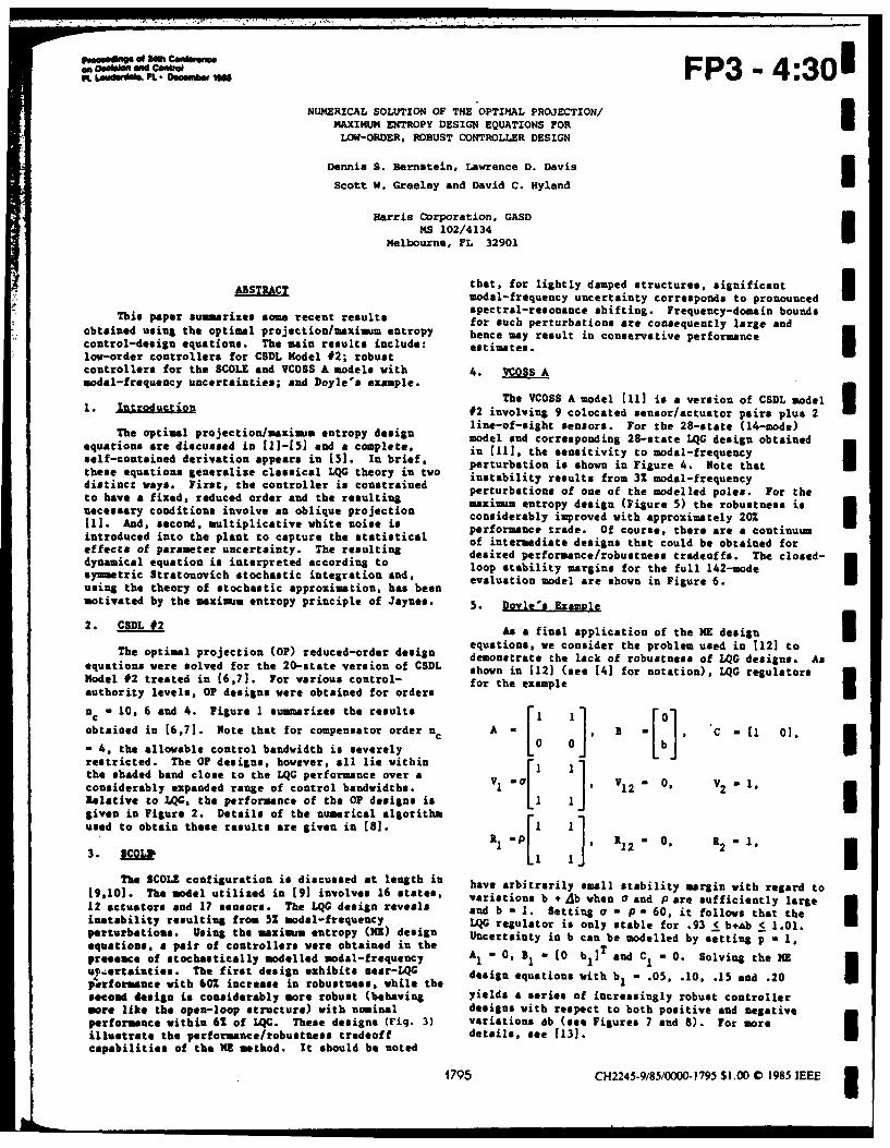
ZSFP3 - 4:301NUMERICAL SOLUTION OF THE OPTIMAL PROJECTION/

MAXIMUM ENTROPY DESIGN EQUATIONS FORLOW-ORDER, ROBUST CONTROLLER DESIGN

Dennis S. Bernstein, Lawrence D. Davis

Scott W. Greeley and David C. Hyland

Harris Corporation, GASDM4S 102/4134

Melbourne, FL 32901

that, for lightly damped structures, significant IABSTRACT modal-frequency uncertainty corresponds to pronounced

spectral-resonance shifting. Frequency-domain boundsThis paper summrizes some recent result. for such perturbations are consequently large andobtained using the optimal projection/maximum entropy hence may result in conservative performancecontrol-design equations. The main results include: estimates.low-order controllers for CSDL Model #2; robustcontrollers for the SCOLE and VCOSS A models with 4. VCOSS Amodal-frequency uncertainties; and Doyle's example.

The VCOSS A model [111 is a version of CSDL model1. Intution #2 involving 9 colocated sensor/actuator pairs plus 2

line-of-sight sensors. For the 28-state (14-mode)The optimal projection/maximum entropy design model and corresponding 28-state LQG design obtained

equations are discussed in [11-151 and a complete, in (111, the sensitivity to modal-frequencyself-contained derivation appears in [51. In brief, perturbation is shown in Figure 4. Note thatthese equations generalize classical LQG theory in two instability results from 32 modal-frequencydistinct ways. First, the controller is constrained perturbations of one of the modelled poles. For theto have a fixed, reduced order and the resulting maxim entropy design (Figure 5) the robustness isnecessary conditions involve an oblique projection considerably improved with approximately 202 U[ll. And, second, multiplicative white noise is performance trade. Of course, there are a continuumintroduced into the plant to capture the statistical of intermediate designs that could be obtained foreffects of parameter uncertainty. The resulting desired performance/robustness tradeoffs. The closed-dynamical equation is interpreted according to loop stability margins for the full 142-modesymmetric Stratonovich stochastic integration and, evaluationIodel are shown in Figure 6.using the theory of stochastic approximation, has been

motivated by the maximum entropy principle of Jaynes. 5. Dovle's Examle

2. CSDL #2 As a final application of the ME designequations, we consider the problem used in [121 to

The optimal projection (OF) reduced-order design demonstrate the lack of robustness of LQG designs. Asequations were solved for the 20-state version of CSDL shown in (121 (see [41 for notation), lQG regulatorsModel #2 treated in (6,71. For various control- for the example Lauthority levels, OP designs were obtained for orders

nc .10, 6 and 4. Figure 1 sumarizes the results1 B [ 0-C l 0 ,obtained in 16,71. Note that for compensator order nc A - B C - [l 01,

- 4, the allowable control bandwidth is severely 0 0 [restricted. The OP designs, however, all lie withinthe shaded band close to the LQG performance over a VV 0considerably expanded range of control bandwidths. 1 012Relative to LQG, the performance of the OP designs isgiven in Figure 2. Details of the numerical algorithmused to obtain these results are given in (8].

3[. ]O R -1 0, R 2 -1,

The SCOLE configuration is discussed at length in have arbitrarily small stability margin with regard to19,101. The model utilized in 191 involves 16 states, variations b + Ab when o and P are sufficiently large12 actuators and 17 sensors. The LQG design reveals and b - I. Setting o - p - 60, it follows that the

instability resulting from 51 modal-frequency LQG regulator is only stable for .93 < b Ab I 1.01.perturbations. Using the maximum entropy (ME) design Uncertainty in b can be modelled by setting p - 1,equations. a pair of controllers were obtained in thepresence of stochastically modelled modal-frequency A1

= 0, 1 - [0 bl]T and C1 - 0. Solving the Eum.ertainties. The first design exhibits near-LQG design equations with b1 - .05, .10, .15 and .20pIerformance with 60Z increase in robustness, while thesecond design is considerably more robust (behaving yields a series of increasingly robust controllermore like the open-loop structure) with nominal designs with respect to both positive and negativeperformance within 61 of LQG. These designs (Fig. 3) variations Ab (see Figures 7 and 8). For moreillustrate the performance/robustness tradeoff details, see 1131.capabilities of the ME method. It should be noted

1795 CH2245-9/85/000-1795 $1.00 0 1985 IEEE

COMPONENT COST ANA *CI IC..+ .,s

I!&XI6.

-. f"S 103 ERROR DEGRADATION 5

K 04UNSTABLEPU~ O C<,

COSIO "I"T OST 03S

Figure 1 2

Optimal Projection Designs (Shaded Band)

versus Suboptimal Methods 26

AU :: 05 -I S # 1' 2

0A3. ROMA FRECTUbhT PfRTUpgATION

U Figure 3U . - -- -LQG and Maximuim Entropy Designs for SCOLE:

U : Closed-Loop Robustness to Modal-Frequency

W - Perturbations

Figure 2Optimal Projection Performance3 Relative to LQG

1796

VEOS A.COd1LER 2161TVITY

71.1

LOS IFAMUi

Figue V0. r0s .F

Fiigure 6LQGDeignfo VCOSS A: Cloesgn:Sd-LityMagpSet. I

LOStns tEWdA -rqecyPruraiWRO AN ~MAt~ ~IT

500. 0

1.3 1.1

FFigure 6

Kaz'* Enrp DeinfrVCOSS AN e g: Sablt IriCloedoro Robu-ttate tode

Moal ieqcy etubtin

LOS IV97

REFERENCES

3 b00.2 b1..15 b1..1 b1..05 1. D.C. Hyland and D. S. Bernstein. "The Optimal

300 Projection Equations for Fixed-Order Dynamic

Compensation," IEEE Trans. Autow. Contr.,Vol. AC-29, pp. 1034-1037, 1984.

2SO 2. D. C. Hyland, "Application of the MaximumEntropy/Optimal Projection Control Design

Approach for Large Space Structures,"

Proc. Lare Scale Antenna Systems Technolosy

200- Conference, pp. 617-654, NASA Langley,December 1984.

3. D. S. Bernatein and D. C. Hyland, "Optimal

150 Projection/Maximum Entropy Stochastic Modellingand Reduced-Order Design Synthesis," Proc. IFAC

Workshoo on Model Error Concepts and0Compensation, Boston, MA, June 1985.

4. D. S. Bernstein and D. C. Hyland, "The Optimal

Projection/Maxima Entropy Approach to DesigningLow-Order, Robust Controllers for Flexible

S tructures," 24th IEEE Conf. Dec. Contr.,Fort Lauderdale, FL, December 1985.

5. D. S. Bernstein and D. C. Hyland, "The Optimal

Projection Equations for Reduced-Order Modelling,I........ .... F Estimation and Control of Linear Systems with

.7 .9 1.0 1. 2 1.3 Stratonovich Multiplicative White Noise,"submitted for publication.

b+ab (Actual Value) 6. R. E. Skelton and P. C. Hughes, "Modal Cost

Analysis for Linear Matrix Second-Order Systems,"

Figure 7 J. Dyn. Sys. Mess. Contr., Vol. AC-29,

Robustness for Doyle's Example: pp. 520-530, 1984.LQ plus ME DesignsSp7. A. Youauff and R. E. Skelton, "Controller

Reduction by Component Cost Analysis,"IEEE Trans. Autos. Contr., Vol. 102, pp. 151-

1163, 1980.

8. D. C. Hyland, "Comparison of Various Controller-Reduction Methods: Suboptimal Versus Optimal

Projection," Proc. AIAA Dynamics Specialist*1.2 Conf., pp. 381-389, Palm Springs, CA, May 1984.

Upper Bound 9. L. W. Taylor and A. V. Balakrishuan,B"A Mathematical Problem and a Spacecraft Control

Laboratory Experiment (SCOLE) Used to EvaluateControl Lavs for Flexible Spacecraft ...NASA/IEEE Design Challenge," NASA/IEEE Report,

b+ab June 1984.

(Actual_ __le_ 10. L. D. Davis, D. C. Hyland and D. S. Bernstein,

"Application of the Maximum Entropy Design

.05 .10 .15 .20 Approach to the Spacecraft Control LaboratoryExperiment (SCOLE)," Final Report, NASA Langley,

January 1985.

11. J. N. Auburn, C. Z. Gregory, M. G. Lyons,R. L. losut and A. A. Woods, Jr., "Vibration

Control of Space Structures VCOSS A: High andLow-Authority Hardware Implementation,"AJWAL-TR-83-3074, Air Force Wright Aeronautical

Lower Bound Laboratories, July 1983.

12. J. C. Doyle, "Guaranteed Margins for LQG

Regulators", IEEE Trans. Autos. Contr.,Vol. AC-23, pp. 756-757, 1978.

.r7 13. D. S. Bernstein and S. W. Greeley, "RobustController Synthesis Using the Maximum Entropy

Figure 8 Design Equations," submitted for publication.

Stability Bounds for Doyle's Example

1798

I

The Optimal Projection Equations IFor Reduced-Order Modelling, Estimation and Control

Of Linear Systems With Multiplicative White Noise 1 2

D. S. Bernstein3 and D. C. Hyland4 4

Communicated by J. L. Speyer

IIII

1This research was supported in part by the Air Force Office of ScientificResearch under contracts F49620-84-C-0015, F49620-86-C-0002 andF49620-86-C-003 8.

2We wish to thank Jill Straehla for excellent typing of the manuscriptversions of the paper.

3 Staff Engineer. Controls Analysis and Synthesis Group, Government AerospaceSystems Division. MS 22/4848. Harris Corporation. Melbourne. FL 32902.

4Group Leader, Controls Analysis and Synthesis Group, Government Aerospace mSystems Division. MS 22/4848. Harris Corporation, Melbourne, Florida 32902.

I____ , -.... ,..' , . ..- ,.. . ... ,,, -.. ,-; ,% ... ..... . . .......... .... ... ... . . ...... .

IItl_

II Abstract. The optimal projection equations for quadratically optimal reduced-

order modelling, estimation and control are generalized to include the effects

I of state-, control- and measurement-dependent noise.

I Key Words. Feedback, control, robust, fixed-order, optimal.

I

IIIII

IIIII

I

1. Introduction

As is well known, LQR and LQG controllers lack guaranteed robustness Iwith respect to arbitrary parameter variations (Refs. 1 and 2). A widely

studied approach to correcting this defect involves introducing noise into the Iplant via the imperfectly known parameters (Refs. 3-10). Intuitively speaking.

the quadratically optimal feedback controller designed in the presence of such

disturbances is automatically desensitized to actual parameter variations. This

was demonstrated in Ref. 11 for the example given in Ref. 1.

The contribution of the present paper is a generalization of classical

steady-state LQG theory to include the effects of state-, control- andm

measurement-dependent noise. In contrast to the classical solution involving a

pair of separated Riccati equations, the necessary conditions for quadratic

optimality in the presence of multiplicative white noise consist of a system of

two modified Riccati equations and two modified Lyapunov equations coupled by

stochastic effects. The coupling serves as a graphic portrayal of the breakdown

of the separation principle in the multiplicative noise case. When the

multiplicative noise terms are set to zero, the modified Lyapunov equations drop

out and the modified Riccati equations immediately reduce to the standard pair

of separated LQG Riccati equations. Related results were obtained for the

discrete-time, finite-interval problem in Ref. 10.

To attain further generality, a constraint is imposed on controller

order as in Ref. 12. Hence. the results of the present paper also constitute a

direct generalization of the coupled system of modified Riccati and Lyapunov

equations which arise in characterizing reduced-order controllers.

For the special case of full-order compensation in the presence of

state-dependent noise only. versions of these equations were discovered

independently by Hyland (Refs. 13 and 14) and Mil'stein (Ref. 15). An

interesting difference between Refs. 13 and 14 and Ref. 15 is that Mil'stein

interpreted the plant model as an Ito stochastic differential equation whereas

Hyland utilized the Fik-Stratonovich definition (Refs. 16-18). In earlier work

on modelling flexible mechanical structures (Refs. 19 and 20). justification for

this interpretation as an appropriate model for parameter uncertainty was based

1!

m upon the Maximum Entropy Principle of Jaynes (Ref. 21) and the theory of

stochastic approximation (Ref. 22). A summary of this approach end its

relationship to Refs. 23 and 24 can be found in Ref. 25. Rigorous guarantees of

robustness over a prescribed range of parameter variations have been obtained

using Lyapunov functions (Refs. 26-29). Although the present paper utilizes an

Ito model for simplicity, results based on Stratonovich models are readily

obtained by means of standard transformations.

An immediate practical benefit of the structured form of the necessaryconditions is the means for constructing numerical algorithms which differ

fundamentally from gradient search techniques. One such iterative algorithm.

proposed in Refs. 30-32. exploits the characterization of the oblique projection

as the sum of rank-1 eigenprojections of the product of the rank-deficient-pseudogramians" satisfying the modified Lyapunov equations. As discussed in

Ref. 32, the necessary conditions fail to specify which eigenprojections

comprise the oblique projection; indeed, each choice may correspond to a local

extremal. In practice, judicious choice of the eigenprojections can eliminate

extremals with high cost and hence efficiently identify the global minimum.

These issues are a result of the reduced-order constraint only; the stochastic

effects alone do not appear to introduce extremel multiplicity.

The scope of the present paper involves deriving the optimal

projection equations for reduced-order modelling, estimation and control

obtained in Refs. 32. 33 and 12 to include state-, control- and measurement-

dependent noise. The main results, Theorems 2.1-2.3, present the necessary

conditions for optimality as systems of 2. 3. and 4 matrix equations (modified

Riccati and Lyapunov equations) coupled by both the optimal projection and

stochastic effects. The necessary conditions in this generality are presented

here for the first time. The dynamic compensation result supports the numerical

3 results obtained in Refs. 11 and 34. Appendix D contains the proof of Theorem

2.3; the proofs of Theorems 2.1 and 2.2 are similar and hence are omitted.

m Although the derivations in Refs. 32. 33 and 12 utilizing Lagrange multipliers

could have been adapted to the present case, we have devised a new proof based

3 upon Kronecker products which is thought to be more direct.

2

~I

2. Problem Statement and Main Results

the paper.The folloving notation and definitions vill be used throughout

Z expected value

R real numbers 3e x p Qx3 real matrices

Ia Ckxa identity matrix

Z W ith element of vector Z

z(ij) (ij) element of matrix Z t

ZT transpose of vector or matrix Z

Z-T (ZT)-I or (Z-1)T

O( Z) rank of matrix Z

tr Z trace of square matrix Z

1

IlzIJ (tr ZZ T) (Frobenius norm)

diag(a1 , f. act) CYxC diagonal matrix vith listed diagonalelementsI

E. matrix with unity in the (ii) positionand zeros elsevhere

2. 2.X. (1,l) Yz X. -1

X Y YI

xc, )Y .Rx(4,5 xR (Kronecker product. I

Ref s. 35 and 36)

3

I y XeIp + I0Y

ZE.&a xa, Y e (Kronecker sum)

3Z group generalized inverse (Ref. 37)

row,(Z) ith roy of matrix Z

coli(Z) ith column of matrix Z

n ve Cz lag, Z e Raxf

L Colo(Z) j

Z (1) . . . Z ].alr:<'"" <<<--'>* W LE.,,<> Z GRaft

vec~ (L . . ]a) Z

stable matrix matrix with eigenvalues in open left half* plane

nonnegative-definite matrix symmetric matrix with nonnegativeeigenvalues (Z O)

n positive-definite matrix symmetric matrix with positiveeigenvalues (Z >0)

semisimple eigenvalue eigenvalue with equal algebraic andgeometric multiplicity

3 simple eigenvalue eigenvalue with unity algebraic

multiplicity

group-invertible matrix matrix Z satisfying p(Z) - p(Z2),

i.e., matrix which is either invertibleor whose zero eigenvalue is semisimple(Ref. 37)

semisimple matrix matrix with semisimple eigenvalues(i.e., nondefective matrix)

I real-semisiple matrix semisimple matrix with real eigenvalues

nonnegative-semisimple matrix semisimple matrix with nonnegativeeigenvalues

I4

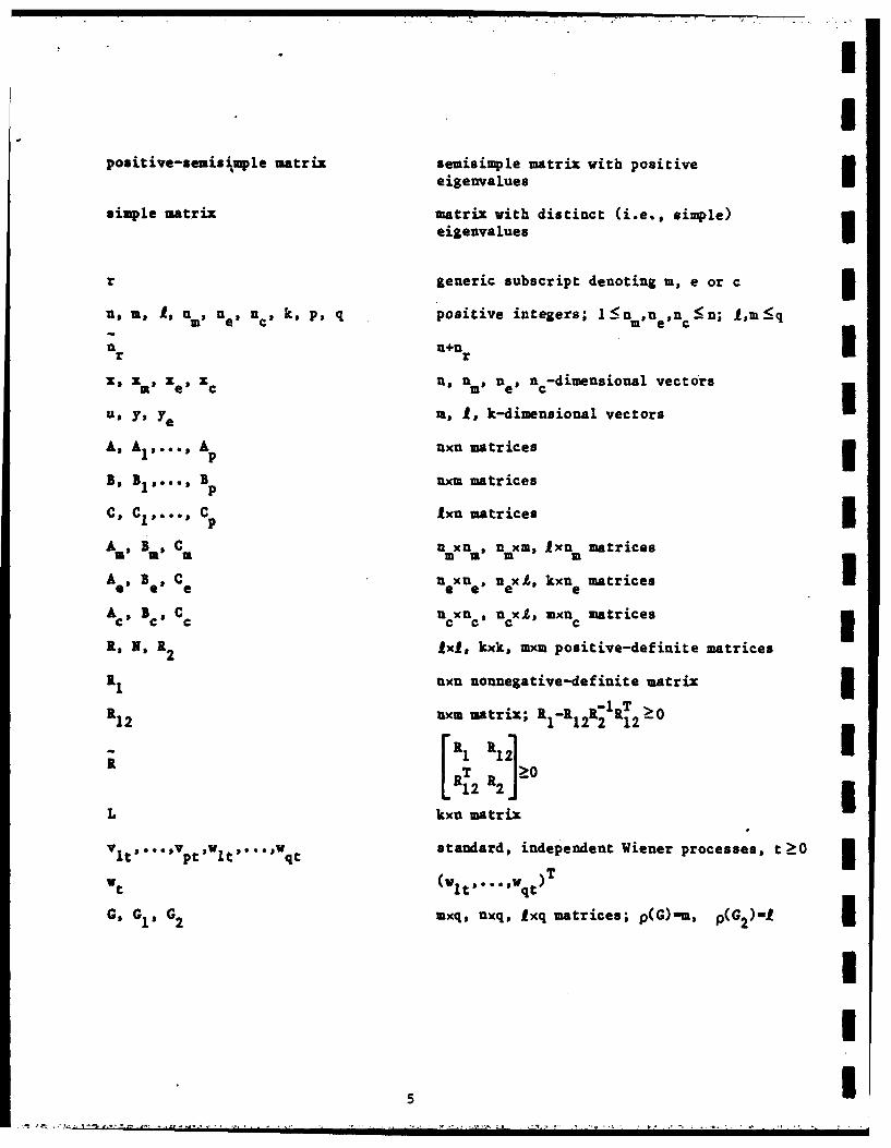
~I

Ipositive-semisimple matrix semisimple matrix with positive

eigenvalues

simple matrix matrix with distinct (i.e., simple)

eigenvalues

r generic subscript denoting m, e or c 3, 1, n a , he, nc, k, p, q positive integers; 1nM,n e,n cn; I,m_5q

n n+nUnr Inr I

x, x, Xe, xc , ne , nc-dimensional vectors

u, y, Ye M, 1, k-dimensional vectors

A, A1 ,..., A uxn matrices 3B, B1 a..., Bp nxm matrices

C, CI,..., Cp Ixn matrices 3An, B ,C mxnm . nMxm, ixn matrices

Ae , B, Ce eXn e , n eX1, kxu e matrices I

A€ , B € , Cc UcXn c , nCx2, mxn c matrices 3R, N, R2 ixl, kxk, mxm positive-definite matrices

1 nxn nonnegative-definite matrix 3R12 uxm matrix; RI-RI2R2 aT >0

-12]

12

R RT R >20

L kxn matrix

V It, • .,VptWit,.e 8 ,qt standard, independent Wiener processes, t20 3Vt (wit, 1..9wqt ) T

G, GI, G2 mxq, nxq, .xq matrices; p(G)'m, p(G2)-i 3II

5

11G T V G GT >0 V GGT >Q.

I GI 11O "12 12 2 .22'

3 - F~ il G - [: 0,Bk [i kn 0J 'in 0]

G 3, B CB, G BG,a, e.. e c c

v -, i aiVBT ;- v B- VB3r .r.r m m m e e e c c c

c kEcC 1c, C e [L -Ci 1,1P, C CCc

A 3 A. A [+ ]E A i [0 Air]

A A A e 3 A. cA..I Ir e e- Ii c

1 6

II

i i-IUsing o the olo win efintion s lecnsa e t Qec ore Poelig Qiato PI

and Toto prblTs

R2t " Rxtd + B i (PPA~xd. + 2lvt V(1 r ( )

~QC + V + ~ T T T

12+E A i(Q+iQ)C, i BP R 1 + Z B.i(P+P)A.,12il 12 i I

AQ 'A- g^'C A A -BR 1 P.Q V2c2.

Using the above notation we can state the reduced-order modelling, estimation

and control problems.I

Reduced-Order Modellin-2 Problem. Given the nth-order model3

yt Cits (2)I

where t e [0, rc), determine an n Mth-order model

dzt -A z dt+ B Gdwt, (3)

ymt m x i, (4)3

which minimizes the model-reduction criterion

J a(A MB MCm) = lir sup 9[(Yytj),R(yt-Ymt)A. (5)

7 I

Reduced-Order State-Estimation Problem. Given the nth-order observed

system

I pdxt Ax tdt +. LA ix dv. +.BGdwt, (6)

pdyt -Cxtdt + Z C ix dv.i 2dt (7)

where t e [ O.) des ign an uneth-order state estimator

dxet mAex t dt+B dy t' (8)

Yet m C xt (9)

1 which minimizes the state-estimation criterion

J J(A B ,C) lim u (x- T x- M.10e e e e. t-'0 =L~~~ t(z- ] (10) e

I Reduced-Order Dynamic-Compensation Problem. Given the nth-order

observed and controlled system

p pdxt M Ax dte + ZAxtdv~t + Bu dt + LBu dv.t + G 1dvt, ft11)

pdyt -Cxtdt + X Cxdvt + G. dvtb (12)

i-lI t it

3where t e [Ooo), design an n cth-order dynamic compensator

zct -Ac xct dt+Bc dtt(3

Ut M C x , (14)

I 8

I

which minimizes the dynamic-compensation criterion

(A 'B 9C) limr sup I T R xT u T Ru(5,Cc C ExTRxt+ 2xTR12ut + uTR 2 ut]. (15)

Clearly, J m Je and J are nonnegative, extended-real-valued

functionals defined on appropriate Euclidean spaces. Explicit expressions forthese functionals are now given. Henceforth we assume that E 2 and that

XrO and vlt,...v ptwt are uncorrelated, t?0.

Provosition 2.1. The nonnegative-definite covariance I%(t)A E[XrtXrt], t>0, is given by

Qr(t) = AQ(t).+ Qr(t)Ar + t .i+ Vr& t >o. (1)

or, explicitly, by !

Qr(t) = vec (e vec, Qr(O) + fe d vec Vr) (17)Inr' nrl 0

The cost criteria Jas Je and Jc are given by U,r(Ar.B rCr) = lim sup tr Qr(t)rr, (18) 3

or, equivalently, by 3" T Art e -

Jr(A.Br.C)lim sup (vec Rr) (rvec Q(O) + f ~vcV r).(19)t- +G 0

Proof. See Appendix A. 13

U

9 I

II

The finiteness and smoothness of Jm Je and J clearly depend upon the

interrelationships among Q r(0). A Rr and V r To avoid a detailed analysis and

to guarantee that JM& Jet and Jc are finite and independent of initial data. we

restrict our consideration to second-moment stable or second-moment stabilizing

design triples. Furthermore, to avoid degeneracy in later developments (and

without loss of generality) only minimal (i.e., controllable and observable)

realizations are admitted. Hence, for the modelling, estimation and control

problems define the open sets

S = [(A ,B .C ): A is stable and (A B C ) is minimal).-r r r r -rr

In the following result we abuse notation slightly and let Qr denote lim Qr(t).

Proposition 2.2. Suppose S is nonempty. If (A r,B rC r )e S then -•-r rrr -rr

lim Qr(t) exists and is given by the unique, nonnegative-definite solution to

--T P - (0

3 or, explicitly, by

r rvec.- (-A rvec V) (21)(n r n r )

Hence,

SJr (Ar B *Cr) = tr QrR r (22)

or. equivalently.

ir (ArsB ,C) -(vec R Avec V. (23)

I

*, , r r r - r

II

Proof. See Appendix A. 0 3As a side note ve examine the evolution of the mean value of x

Proposition 2.3. The mean

m(t) rt, t2.0, (24)

satisfies

3(t) Arm(t). t 2O . (25)

Furthermore, if (A rB rCr) e Sr then Ar is stable and thus

lim m(t) - 0. (26)t-oo IProof. See Appendix A. 0

Of course, it is useful to know vhen the sets Sm, Se and S are 1

nonempty. Although for the closed-loop control problem the question is complex

because of stabilizability concerns, the modelling and estimation problems

permit considerable simplification.

Proposition 2.4. S (alternatively, W8) is nonempty if and only if

A is stable. In this case S and S are given by I

S= {(A ,B ,C m): Am is stable and (A m,Bm C ) is minimal},

S " ((Ae,B eCe): Ae is stable and (Ae,BeC e ) is minimal}.

111

i .| l. . - ,

Proof. See Appendix B. 0

The following observation concerns the smoothness of the

cost functionals.

IProposition 2.5. The functionals J rare infinitely Frechet

differentiable on

Proof. From Lemma 3.7.2. p. 203 of Ref. 38, it follows that the mapWW - defined on the set of invertible matrices is C0. The result follows from

the chain rule and (23).

It is now possible to proceed with the principal aim of the paper

which is to characterize solutions of the reduced-order modelling, estimation

and control problems by means of a first-order variational analysis. To this

end, one additional assumption is required. In order to obtain closed-form

expressions for extremal values of the closed-loop control gains, the dynamic-

compensation problem requires the technical assumption

[Bi 0 0 =-> Ci - 0], ii,..., p, (27)

or, equivalently,

I [Ci 0 0=> B. = 0], i-0,..., p, (28)

i1 "i.e., for each i E {1,...,p}, Bi and C. are not both nonzero. Essentially,(27). expresses the condition that the control-dependent and measurement-

3 dependent noises are independent. There are no constraints, however, on

correlations with the state-dependent noise.

I In order to state the main results we require some additional notation

and a lemma concerning a pair of nonnegative-definite matrices. For a real-

semisimple matrix X .ex define the set of diagonalizing matrices

I

I 12

UXUand, for a pair of nonnegative-definite matrices X, Y 1E RUf define the set of

contragrediently diazonalizing matrices

C(X~Y) O l fxfl: *-l z T and 4T~are diagonal)

and the subset of balancing transformations

B(X.Y) A J* ECX.Y): q'- lfT = 4 y*

The following result unifies and extends similar results found in Ref s. 32, 33

and 12.

Lemma 2.1. Suppose Q, Pe R~ are nonnegative definite and

POQP) - u1 r* Then the following statemnents hold:

Ci)0 #C(Q,P) C D(QP).

(ii) QP is nonnegative semisimple.

(iii) The nxn matrix

-r aa aa^(QP# (29)3

is idempotent, i.e., Tis an oblique projection.

(iv) There exists *I'eC(Q,P) with (*'QPi')(.) 0, iinl,...,n r such that

'r is given by

n r

n = l(Qs. (30)

(v) If p(Q) -p(P) - n r then B(Q,P) #0.

13I

I(Vi) if P(Q) -P(P) -n then there exists 4e B(Q,P) with

('i'QP )(ii) r 1,.j.ln;, such that T is given by (30).

U (vii) If p(Q) - p(P) n r then

IE^aQ T . TT - J Ta1

IP P'TT - T PT. (32)

I -., T ., ,,c.

(viii) There exist G, e R and positive-semisimple Mc R such that

aa TQP -G HI;. (33)

i rGT I 1I . (34)

. n xn n xn(ix) If G, e r and EH R satisfy

IP a = .(35)

r -T 1 (36)i m Inr'

then there exists invertible S R r r such that s-TG, r - Sr and R - SMS- 1 .

1xn fl, lxn

(x) If G, r e r and M e r rsatisfy (33) and (34) then M is

invertible. (QP) " GT-r and

I C rTr. (37)

I Proof. See Appendix C.

14

For convenience we shall call G, re R rx and M en ~r nr satisfying3p.a

(33) and (34) a Projective factorization of QP. Furthermore. define thecomplementary oblique projection3

.L iIn T (38)3

and let J(A 'B C r) denote the Frechet derivative of Jr evaluated at

(A r B r 'C r).I

It is now possible to state the main results, which provide a3

parameterization of triples (A r iBr 'C r) S rfor which the first Frechet

derivative of J vanishes.

r

Theorem 2.1. Assume A is stable. Then. for (A B.mC m) e S IJ-(A B C) 0 (39)Ia m mU

if and only if there exist nxn nonnegative-definite matrices Q and P such that,for some projective factorization G, m, r' of QP, Am, B and C are given by

A m= rAGT. (40)1

B a-I'D, (41)I

Cm M.CG T (42)3

aT

and such that, with 7 QP(QP) -G r' and T Ij h oloigcniinn I

are satisfied:

15

t

Q=A+QA +BV (43)(Q + T + cVT- TICTRCTJ,

-pP ipQP) (5

Furthermore, if (A ,BaCm) E Sm satisfies (39) then the extremal cost is

I given by

J am(A , B Cm ) = tr[(WcQ)CTRC]

- tr[(W -P)BVT] (46)

2tr((QP-W W ),A,] 2 trW A

where W, W eR n Xn are the unique, nonnegative-definite solutions toI o

0=AW +W AT, T T+ B( (47)

3c C MA.IA+3VI

U 0= AW + WA + P T .+CR.(48)~ 0 Al- 1 0 1

Theorem 2.2. Assume A is stable. Then, for (Ae.B eCe) Es

Je(AeBeCe) - 0 (49)

e a a

if andonly if there exist nxn uonnegative-definite matrices Q, Q and ; such

that, for some projective factorization G, x, r of QP, Ae B and C are

given by

I1

Im

A = r(A~gA-lC)GT. (50)1

B rg;V'. (51)

Ce- LGT, (52)

and such that, vith T9 QP(QP)* G r and , 9 In- , the following conditions

are satisfied:

TAT T, -- 2 + a1TT (530 AQ + QAT + V1 + IAi(Q4)A - 9V2 9 +i9V 2 . (53)

+0^_ T _Q T 9TA V2 9 - 1qV2 '1-~ (54)I

0A P + PAQ + L 141 - ILNT.(5

P(Q) - P(P) - a(P a (56)

Furthermore, if (A~ e BeC e) e satisfies (49) then the extremal cost is

given by

J e(A e,B ,Ce) - tr QLTNL. (57)

Theorem 2.3. Assume (27) holds and S is nonempty. Then for I

JI(Ac,'cC) B 0 (58)

if and only if there exist nxn nonnegative-definite matrices Q, P, Q and P such

that, for some projective factorization G, m, r of QP, Ac , B€ and Cc are

given by

II

. . . . . . .. " " ' ". ' i" ' , I I i ' i -l' .... . . .. .... . . ." ...1 7. I . .. I

I.I

r(Ao.A = (A-BR2 1 22C )GT. (59)

= 1 (60)

TT V

-R2 1 .P , (61)

and such that. with TA QP (QP) =Gr rand TI= T the following conditions

I

are satisfied:

I T .- -l T ^-19T, ~-12T T.0= AQ+Q I + [A QA +(A 2P)2 A. - ) R P)(62)=1R 2 )QA-B.R 2 ]-9V2 + + T (62

0 FterI [A iPA +(A-2v2 CC _S P(A s is-V 2 C) R 2 +Tl I oPRt (63)

Ii=

o=~+~ 4 T ^-l T ^9 -l9TT(4

0 =~ T1 0A+ PAQ +PR P- PT7f2 (65)

:. -,. / ,, .Q. .. .... - 2 - . ,j,

P(Q) = P(P) p(QP) = n .. (66)

I Furthermore, if (A.B.C,) eS Csatisfies (58) then the extremal cost isgiven by

J(AcP~C~)2 tr[(Q.Q)R 2RR1C C Tc1 12-2lK

T+P R -RPQJ (67)

I 18

3. Appendix A: Proof of Propositions 2.1. 2.2 and 2.3

First note that (1)-(4). (6)-(9) and (1l)-(14) can be written as

dx rt2-Arztdt + Ax dv.t + G rdvt (68)

From Theorem 8.5.5, p. 142 of Ref. 17 (or from the Ito differential rule) it

follows that the nonnegative-definite covariance Qr (t) is given by (16).

Furthermore. (5) * (10) and (15) are equivalent to (18). Rewriting Q rt) in the

form (see Refsa. 35 and 36)

vec Q r(t) = A rvec Q r(t) + vec Vr (69)

leads to (19).

To prove Proposition 2.2. note that the stability of Ar implies,

by (69), that Qr A lir Q r(t) exists and is given by (21). which satisfies (20).St- O

Clearly. Qr Z 0 since Q r(t) > 0, t Z 0. Now (22) and (23) follow from (18) and

(19). 0 ITo prove Proposition 2.3. note that the differential equation for M(t)

is an immediate consequence of (68). To show that Ar is stable, we proceed as

in Lemma 2.2 of Ref. 4. Repeating the steps leading to (22) with V replaced by

I; it follows (see Ref. 4) that (A I1- ) is stabilizable. Hence.n r n

r r

t ; TI er er da0 •~ do"

in bounded as t-.m. which implies Ar is stable. 0 I

19I

II

4. Appendix B: Proof of Proposition 2.4

We require some elementary properties of the Kronecker product (Refs. 35

and 36) applied to partitioned matrices. For Xe Rs t and Y e Rp q partitioned by

t I t 2 ql q21 X 1 [ 2 "Y 1

it follow: that

XO x1 1 Y X12 0 Y

I - xI@0I 121 yx

0 U a X J OX 21 YO ® 2 U qxt2

"Y1 eX 1 Y1 2 ®X 1 Y1 eX1 2 Y1 2 ®X 1 2

whr U 0 3 Er®" Y Y Y:e12j ex Ut Iqt0

[ :2P YI OX21 Y1 2 ®X2 1 Y1 OX 2 Y1 2 ®x2 0 UqXt J

Y2 1 ®X21 Y2 OX 21 Y2 1 OX 2 Y2 OX2

where U .i is the permutation matrix defined in Refs. 35 and 36. Since Uixj =

Ui1 (i.e.. U is involutory), the stability of (square) X@-Y is equivalent toIixj ixjthe stability of the above block 4x4 matrix. Hence note that

I

I 20 i,! I I

II

A= block-diagonal (AA e A A ) A.A 0 A).

If (A, BM.C) is such that AM is stable then clearly A is also stable and, byelementary properties of the Kronecker sum. A, is stable. Conversely. if A and

ma

A are stable then A is stable. The result for A is obtained analogouslym .- M -enoting only that A is lower block triangular.

-e

5. Appendix C: Proof of Lemma 2.1 I

(i) From Theorem 6.2.5, p. 123 of Ref. 39. it follows that there exists an 3nxn invertible matrix %P such that the nonnegative-definite matrices

D' 9 *-1^-T and D -APTP are both diagonal. Hence C(Q,P) 0. Since

QPD WQi also diagonal, C(Q,P) C D(QP).Q AP

(ii) Since QP = 4A "1, where A A D--D is nonnegative diagonal, QP is

nonnegative semisimple. I

(iii) Since QP is semisimple, it is group invertible. By properties of the

group inverse (Ref. 37. p. 124). T 2 T.

(iv) Note that by means of a basis rearrangement, it can be assumed that 'I'

in U) is such that A- diag(X1, X ,O9...,0), where

QP (D i i) 0, Hence, since A diag(N A n ,0,...,

nr=QP(QP) = *AA* PE.*

i=1 IUII

23.

(v) Since p(Q) p(P) -p(QP), it follows that (D^) 0

(DI)(i,i) # Os '-l,*.n r . Hence, let A and A; denote the upper left positive-m diagonal blocks of D^ and D^, respectively, and define

It now follows that

l oA;) 3 (70)

asTdesired.

(vi) This is an immediate consequence of (70).

m (vii) This is an imediate consequence of (70) and (30)

(viii) With *as in (iv) and Ao9 diag(T . mrn )* it follows that for

fnXnrm arbitrary invertible S 4 R ,

T -1- -1-

-#P AFsO -l -

and thus (33) and (34) hold with G - [S T 01, M - S1 AoS and r - [S "I 014 - ' .

(ix) The result follows from S - R-IrGTM- I with S"1 m M f - I .

(z) The result is a consequence of (viii) and (ix).

I

" "" • , m , t -, * 22

I

6. Appendix D: Proof of Theorem 2.3. I

First note that by arguments similar to those used in Appendix A the dual

of (22) given by

O =AIP + P -T RP(71)r r r r ri r ri r (71)

has a unique. nonnegative-definite solution given explicitly by

-- -1 - (72 'IP r "=vec(.. - ) (-A vec R). (72)

n r " n rI

Define the partitionings

a nr n nr

r r" nj -lq2 n - P1 2

U Q;Q2n - P 1P1 2 ]%r T r P T P-.nr [Q 2 Q2 Jr 12 2.

where, for notational convenience, we suppress the subscript r. Also define the

notation 3- -ZlI Z 121

where

z P1 Q + P QQT 2 P% +

Z PT T Z Q P

21 12l + P2Q12' 2 12Q12 + P2q2

n xn n xA xnand let ( 6 C c c x R x R We now specialize to the

control problem.

III

23

I

Lemma 6.1. Under the assumptions of Theorem 2.3,

J'(A B ,C )(6A .6 )" 2tr[Z2 ] (73)

ccc c A B 16C ~ 26ASC C C C

2tr(VBP + CZ ) I

2+tr[(QC R + Z B + Q [R + A.P B "2T 1 ~2 12 12 . 1B ]

Proof. From Lemma 3.7.2. p. 203 of Ref. 38. it follows that the Frechet

derivative of the map W - W- I is given by 6 --W-1 6wW . Also, recall from

I Refs. 35 and 36 the identities

3 (vec X)Tvec Y - tr xTy,

(X®Y)vec Z - vec YZXT

Hence, using (23) and noting that Vc and R0 are independent of AC, we compute

C A Cvecl ) A A vecS( (A v-T " ) 0 ) ly'ecS A 6 6A

(* - (A- +e In-([ £5A][ 6

U -(vec c )( 0 a 0[ i0 k]

U- Ztr Q ~ 00 0

W 2tr Z TA

I 24

Furthermore, noting that

vecVi vecBV i ii (B 0 B )vec V,

we obtain

8J (A c ,B 'C) T(6B (vec P )TCc

~c c c1

-~~ (ve P) &c

-(vec ; )T([cC 0] * [Bc gjj1 A.i

0 0 r2t (ve 6)( 0 i- j 6B]C 0

- ~ 2tr ;_T 2t 0c J [I Be]

=2trCZ T 6 + 2rp(QATP CJT)21 B r (. 1 A3.12 +C.

+ 2tr(Tp+ V B T )6V12 12 2 c 2B

2tr(V 2 P + ZT1 + [Vp CQA!]P MD6

25

II

A similar computation for (WJ (Ac c.C c )/aCc)6C yields (73).c

We can now proceed with the proof of Theorem 2.3. Obviously. (58)

is equivalent to

0 Z2 . (74)

TT p (750 = P2BcV2 21 2(V12 + iQjCi). (75)

T T P T0 R CcQ + B Z12 + (R 12+ BP 1 A i)Q 12 ' 76

Expanding the nxn. nxn and n cXc blocks of (20) and (71) yields•c c

0=AQ1 + QA T + V + BCQ + Q(BC)

01 QA 1 c 12 12 c(7I (77)

p T T TT T TI A.Q1A. BiCcQi2Ai + IiQ 12.. c c23.(B.C ) + BC Q(B.C)

0 A + AT + BC q, + QBC)T(78)

pT T+ A.Ql(B C.)i + V10c

ATAQ + B ~CQ + Q (BT + B V B (79)c Q2 Ac + Cc)c12 V

0 = ATV1 + PA + R1 + (BC) TP 12 + P12 BC1 1(80)

CP . + (BCi T2B C BCci ci l2i +ilP 2c c i P2 c

* 26

0 = ATP12c P + (BcC)TP2 + PBC c

P (81) I

+ i AP IBiCc + R12C .

O=TPT T T I0 AP+ P A + (BC ) P + P1 2BC + CRC ~ (82)

Obviously. V2 >0 and R2 >0 imply V2 >0 and R2 > 0. Next note that1

# 22since (A _B ) is controllable and V2 > 0 it follows that (A +B CQ12Q2 BV 2 ) is Icontrollable. Using Q12 = Q12Q2Q2 (Refs. 39 and 40), (79) can be rewritten as

0= (A +BCQ Q #)Q + A +B CQQ # )T + a T (3+s' frQ ) +BVB (83)iec c 12 2 2 "2 c c 12 2 c2 c

Now. using Lemma 12.2 of Ref. 41 it follows from (83) that is positive

definite. Similarly. P2 is positive definite.

Since R2 P V2* Q2 and P2 are invertible, (74)-(76) can be written as

-1 T -1 (84)i2 P1 2 9 1 2 Q2 = Inc

T T -I

Bc = -P21 1T + P (V + AQ CT)]^ V 2 4 (85)

C=--l ZT T -1 (6-R2 [B 12 (R1 2+_B.P 1Ai)Q 1 2]Q 2 (86)" !I

Nov define new variables-1Q T P -P P 12 IT(7

S Q1 2 2 12 P 1 2P2 1 2 (87)

-1T A P -1 T (88)

Q1 2Q2 Q1 2 ' 1 2 12'

27 I

I.I

which are nxn nonnegative-definite matrices. Note that because of (84), (33)

and (34) hold with

G A Q1 Q T M .4 Q P2 12-P1 (89)q2 1z2' 2 29 2 12'

i where M is positive semisimple since

I 1 1 -1Q2 P2 - Q2 ( QP 2Q2 )Q2

I It is helpful to note the identities

TTrP r, (90)SQ 1 2GGQ 1 2 GTQ2G, 12 12 P2,=(9)2

3 TGT = GT FT=f, (91)

Q = TQ , P M P7, (92)

QT -l2 . (93)IUsing (34) and Sylvester's inequality, it follows that

p(G) = () - p(Q12 ) - p(P1 2 ) - nc which in turn imply (66).

The components of Qc and Pc can be written in terms of Q, P, Q, P, G

IAAQ1 2 . Q + P 1 aPG+1T (95)

TQ2 a r' 8 P 2 - GPG. (96)

II 28

The gain expressions (60) and (61) can now be seen to be equivalent to (85) and I(86). Substituting (94)-(96) into (77)-(82) yields

P T )- BR. ^+l

0= + QAT + V+ 1EAjQAi + (A.-Bi jQAi -BR.P I +i aPQ a T. (7

P T T

0 -ApQ + Q(_TAcG+CT;21T) + 21 T irT. (98)

T a-l a ^ T ^- T ^l

iMG Ar+ 2V2 C)Q+Q(GAI' gV2 C) +9V 2 g r (99)1

0(= ATP + PAr ) + T(PA. + (A.-2V ~ I P i eV p + e As a (100)1=2 -1 3. i 2 i 2 i IPPQ

I

^0 T a + P(G 99) di(1) A rsuRpe e (101)

T a-l T^ a T .-l T^-l T0 = G((G Acr+BR2 f) P +P(G Ar+BR f) + P R21 . (102)

The remaining calculations proceed as follows. Computing either

(90-r08) or (102)-G(101) yields (59). Inserting this expression for A into

(98). (99). (101) and 102 and computing the (equivalent) equations GT(98)T

GT(99)G. (101)r and I..(1 o2)r it follows that GT (99)G = GT (98)TT and rT (102)r NT(101)r Hence. (99) and (102) are superfluous. Furthermore. GT(98)T and (101)r

are equivalent, respectively, to 30 = T (ApQ + A; + 9 ] . (103)• I

0=ASP + PAQ + P RTaP~1 (104)

Finally. to obtain (62)-(65) note that (64) = (103) + (103) T -( 1 03 )-T (62)=3(97) - (64). (65) = (104) + (104) - 'T(104) and (63) = (100) - (65). 0

I

29 i

~~~~ . .. .. - , ..- . : ." • , T .. . ' • . ;. . . . .

I

References

1. DOYLE. J. C., Guaranteed Margins for LQG Regulators, IEEE Transactions

on Automatic Control, Vol. AC-23, pp. 756-757, 1978.

i 2. SOROKA, E.. and SHAKED. U., On the Robustness of LQ Regulators,

IEEE Transactions on Automatic Control, Vol. AC-29. pp. 664-665, 1984.

i 3. WONHAM, W. M.. Optimal Stationary Control of a Linear System with

State-Dependent Noise, SIAM Journal on Control. Vol. 5. pp. 486-500,

1967.

m 4. WONHAM, W. M., On a Matrix Riccati Equation of Stochastic Control,

SIAM Journal on Control. Vol. 6. pp. 681-697. 1968.

5 5. KLEINMAN, D., Optimal Stationary Control of Linear Systems With

Control-Dependent Noise, IEEE Transactions on Automatic Control.

i Vol. AC-14, pp. 673-677, 1969.

3 6. MCLAWE, P., Optimal Stochastic Control of Linear Systems with State and

Control-Dependent Disturbances, IEEE Transactions on Automatic Control.

5 Vol. AC-16, pp. 793-798. 1971.

7. HAUSSMANN. U.. Optimal Stationary Control With State and Control

U Dependent Noise, SIAM Journal on Control, Vol. 14, pp. 419-444, 1976.

8. BISMUT, J.. Linear-Qmdratic Optimal Stochastic Control With Random

Coefficients. SIAM Journal on Control, Vol. 14. pp. 419-444. 1976.

3 9. MERRIAM, C. W. III, Automated Design of Control Systems, Gordon and

Breach, New York, 1974.

10. GUSTAFSON, D. E., and SPEYER, J. L., Design of Linear Regulators for

Nonlinear Systems, Journal of Spacecraft and Rockets, Vol. 12.

I pp. 351-358. 1975.

II

'"' - '" " ",'' -" ."'" ', "d" ,". . . . - * "u* ", - .°

" .

I11. BERNSTEIN, D. S.. and GREELEY, S. W.. Robust Controller Synthesis Using

the Maximum Entropy Design Equations. IEEE Transactions on Automatic m

Control. Vol. AC-31. pp. 362-364. 1986. 312. HYLAND, D. C., and BERNSTEIN. D. S.. The Optimal Projection Equations

for Fixed-Order Dynamic Compensation. IEEE Transactions on Automatic m

Control. Vol. AC-29, pp. 1034-1037. 1984.

13. HYLAND. D. C.. and MADIWALE, A. N., A Stochastic Design Approach for m

Full-Order Compensation of Structural Systems with Uncertain

Parameters. Proceedings of the AIAA Guidance and Control Conference,

pp. 324-332, Albuquerque. NM. August 1981. 314. HYLAND. D. C.. Mean-Square Optimal. Full-Order Compensation of

Structural Systems with Uncertain Parameters. MIT, Lincoln Laboratory

TR-626, 1 June 1983.

15. MILmSHTEIN. G. N., Design of Stabilizing Controller with Incomplete 1

State Data for Linear Stochastic System with Multiplicative Noise. 3Automation and Remote Control. Vol. 43, pp. 653-659, 1982.

16. STRATONOVICH, R. L., A New Representation for Stochastic Integrals. 5SIAM Journal on Control. Vol. 4, pp. 362-371. 1966.

17. ARNOLD. L.. Stochastic Differential Equations: Theory and IApplications. Wiley. New York, 1974. 1

18. IKEDA. N.. and WATANABE. S.. Stochastic Differential Equations and

Diffusion Processes, North-Holland, Amsterdam. 1981. 119. HYLAND. D. C.. Active Control of Large Flexible Spacecraft: A New

Design Approach Based on Minimum Information Modelling of Parameter IUncertainties, Proceedings of the Third VPI&SU/AIAA Symposium on Large

Space Structures, pp. 631-646, Blacksburg. VA. June 1981.

II

I,I

20. HYLAND, D. C., Maximum Entropy Stochastic Approach to Control Design

for Uncertain Structural Systems, Proceedings of the American Control

3 Conference, pp. 680-688. Arlington. VA, June 1982.

21. JAYNES, E. T., Where Do We Stand on Maximum Entropy?, in The Maximum

Entropy Formalism, Edited by D. Levine and M. Tribus, MIT Press,

pp. 15-118, Cambridge. MA, 1979.

22. WONG, E., and ZAKAI. M., On the Relation Between Ordinary and

Stochastic Differential Equatiops. International Journal of Engineering

Science, Vol. 3, pp. 213-229, 1965.

323. ATHANS. M.. KU. R. T.. and GERSHWIN. S. B.. The Uncertainty Threshold

Principle: Some Fundamental Limitations of Optimal Decision Making

5Under Dynamic Uncertainty, IEEE Transactions on Automatic Control,

Vol. AC-22, pp. 491-495, 1977.

24. KU. R. J.. and ATHANS. M.. Further Results on the Uncertainty Threshold

3Principle. IEEE Transactions on Automatic Control, Vol. AC-22,pp. 866-868. 1977.

5 25. BERNSTEIN, D. S., AND HYLAND, D. C.. The Optimal Projection/Maximum.

Entropy Approach to Designing Low-Order, Robust Controllers for

Flexible Structures. Proceedings of the 24th IEEE Conference on

3 Decision and Control, pp. 745-752. Fort Lauderdale, FL. December 1985.

26. BERNSTEIN, D. S., and GREELEY. S. W.. Robust Output-Feedback

Stabilization: Deterministic and Stochastic Perspectives. ProceedingsIeof the American Control Conference, pp. 1818-1826. Seattle. Washington.

1 June 1986.

1I1

27. BERNSTEIN. D. S., The Optimal Projection Equations for Static and

Dynamic Output Feedback: The Singular Case, IEEE Transactions on 3Automatic Control. to appear. 3

28. BERNSTEIN, D. S., Robust Stability and Performance via the Extended

Optimal Projection Equations for Fixed-Order Dynamic Compensation, m

submitted.

29. RYLAND, D. C.. and BERNSTEIN, D. S., The I.vjorant Lyapunov Equation: 3A Nonnegative Matrix Equation for Guaranteed Robust Stability and

Performance of Large Scale Systems, IEEE Transactions on Automatic m

Control, 1987. to appear. 130. HYLAND, D. C., The Optimal Projection Approach to Fixed-Order

Compensation: Numerical Methods and Illustrative Results, AIAA 21st 5Aerospace Sciences Meeting, paper 83-0303, Reno, Nevada, January 1983.

31. HYLAND. D. C., Comparison of Various Controller-Reduction Methods: ISuboptimal Versus Optimal Projection, Proceedings of the AIAA Dynamics 3Specialists Conference, pp. 381-389. Palm Springs. California,

May 1984. 532. HYLAND, D. C.. and BERNSTEIN, D. S., The Optimal Projection Equations

for Model Reduction and the Relationships Among the Methods of Wilson, 1Skelton and Moore, IEEE Transactions on Automatic Control, Vol. AC-30.

pp. 1201-1211. 1985. 133. BERNSTEIN, D. S.. and HYLAND, D.C., The Optimal Projection Equations

for Reduced-Order State Estimation, IEEE Transactions on Automatic

Control. Vol. AC-30. pp. 583-585, 1985. 3III

.":-;. ;"' "I'',-,-,Il i 'lt~ibm~~ d~~'; ... ..... I........ "..."".....*' " • '" "

I34. BERNSTEIN, D. S., DAVIS& L. D.* GREELEY, S. W., and HYLAND, D. C..

.Numerical Solution of the Optimal Projection/Maximum Entropy Design

3 Eiuations for Low-Order, Robust Controller Design, Proceedings of the

24th IEEE Conference on Decision and Control, pp. 1795-1798.

Fort Lauderdale, Florida. December 1985.

35. BREWER. J. W., Kronecker. Products and Matrix Calculus in System Theory.

IEEE Transactions on Circuits and Systems. Vol. CAS-25. pp. 772-781.

1978.

36. GRAHAM, A.. Kronecker Products and Matrix Calculus. Ellis Horwood.

5 Chichester, 1981.

37. CAMPBELL. S. L.. and MEYER. C. D.. Jr.. Generalized Inverses of Linear

3 Transformations, Pitman. London. 1979.

38. FLETT. T. M.. Differential Analysis, Cambridge University Press,

I Cambridge. 1980.

m 39. RAO, C. R., and MITRA, S. K.. Generalized Inverse of Matrices and Its

Applications, John Wiley and Sons. New York, New York, 1971.

5 40. ALBERT. A.. Conditions for Positive and Nonnegative Definiteness in

Terms of Pseudo Inverse, SIAM Journal on Applied Mathematics, Vol. 17.

1 pp. 434-440, 1969.

£ 41. KREINDLER. E., and JAMESON A., Conditions for Nonnegativeness of

Partitioned Matrices, IEEE Transactions on Automatic Control.

Vol. AC-17, pp. 147-148. 1972.

42. WONHAM. W. M.. Linear Multivariable Control: A Geometric Approach.

i Springer-Verlag, New York. New York. 1974.

1II

TRANSACTIONS ON AUTOMATIC CONTROL. VOL. AC.31. NO. 4. APRIL 198

Robust Controller Synthesis Using the MaximumEntropy Design Equations

DENNIS S. BERNSTEIN AND SCOTT W. GREELEY

Abstruc-Thls note presents an application of the optimialty condi-dons obtained In Ill for dynamic compensation In the presece of state-,control-, and cteasurement-dependent noise. By solving these equations,which represent a fundamental generalization of standard ateady-sateLQG theory, a series of increasingly robust control designs is obtained forthe example considered In (21.

I. INTRODUCTION

Perhaps the most significant aspect of LQG theory is the explicitsynthesis of dynamic feedback compensators. In practice, however, LQGsuffers from serious defects concerning closed-loop robustness withrespect to plant deviations. In particular, LQG controllers may possessarbitrarily small stability margin with respect to parameter variations [21.

One approach to correcting this defect is to rederive the optimalityconditions for dynamic compensation in the presence of state-, control-,and measurement-dependent noise [I]. Intuitively speaking, the quadrati-cally optimal feedback controller designed in the presence of suchmultiplicative disturbances is automatically desensitized to actualparameter variations. The optimality conditions now comprise a system offour matrix equations, specifically, two modified Riccati equations andtwo modified Lyapunov equations, coupled by stochastic effects. This

coupling is a graphic reminder of the breakdown of the separationprinciple in the uncertain plant case. When the uncertainty terms areabsent, the equations immediately reduce to the standard pair of separatedRiccati equations.

For the special case of full-order compensation in the presence of state-dependent noise only, versions of these equations were discoveredindependently by Hyland [31-15) and Mil'stein [61. A crucial feature of[1, [31-[51 is the interpretation of the closed-loop stochastic differentialequation according to the Fisk-Stratonovich definition of stochasticintegration. For modeling flexible mechanical structures, justification ofthis interpretation as an appropriate model for a priori parameteruncertainty was based upon the maximum entropy principle of Jaynes ([1.

A time-varying version of these design equations involving uncorrela-ted state- and control-dependent noise has been given in [7]. Thestochastic interpretation is in the sense of Ito as in (6].

The purpose of the present note is to summarize the maximum entropyequations for full-order dynamic feedback compensation. These equa-tions are then applied to Doyle's example [21 to produce a series ofquadratically optimal robust controllers. The full optimal projection/maximum entropy design equations, which also account for a constrainton controller order 1l). 18]. are applied to a more realistic design problemin [91.

11. PROBLEM STATEMENT AND MAxIMUM ENTROPY DESIGNEQUATIONS

To state the optimal dynamic-compensation problem, we require thefollowing notation. Let x E A1", y E 12', u E Rj, A, AI, "'*, A, Efi", B, B1, B, E 8, , C, C1, " ", C, 6 Al' ", R, E W"-,R > 0, R2 6 lv", R2 > 0. Furthermore, let vl, --, u, be unit-inten-sity. zero-mean, and mutually uncorrelated white noise processes and letw, E Am" and w2 E 111 be zero-mean white noise processes with

Manuscript received July 23. 1995; revised October 24. 1985. This work was 1supported in par by the Air Force Office of Scientific Research under Conmct AFOSRF49620-94-C4]0I 5.

The authors are with the Controls Analysis and Synthesis Group, GoveriamentAerospace Systems Division, Harris Corporation. Melbourne. FL 32902.

IEEE Log Number 8407268.

52$01.00 © 1986 IEEE

U I EE TRANSACTIONS ON AUTOMATIC CONTROL. VOL, AC-31, NO. 4. APRIL 1986 363

i ntensities V, k 0 and V2 > 0. respectively, and cross intensity V12 E B,O., V2.', (2.7)I t" . It is further assumed that v5, wi and x(0) are mutually uncorrelated.We require the technical assumption that, for each i, B, * 0 implies C = (0, i.e., the control- and measurement-dependent noises are uncorrelated. C,= -R I, P,, (2.8)

U pimal Dynamic-Compensation Problem and such that the following conditions are satisfied:

Given the controlled system 0=AQ+ QA T. + V, + IA,QA r

I - (A + j , A)X+ (B+_ vB) u + w,, (2.1) (2.9)

Y.(+Pi~ (22 =AsfP+PA+R,+t [ArPA,

design an nth-order dynamic compensator +(A,-0,V2. ' C,)P(A 1-2s .C 1 )]- 6,R . (2.10)

.j,=A,x,+By. (2.3) 0= Ah+ QA r + CLV'. (2.11)

u=C'r, (2.4)Offi A r .6 + PA C, + 61 rR~j (2.12)

which minimizes the performance criterion (is (2

J(A,, B,, C,)=J,(A,. B,. C)+J4(A, B_, C,)+J,(A,, B.. C,). Remark2.1:LettingA = 0. B, = 0andC = 0, = 1, -. ,pitcanreadily be seen that (2.11) and (2.12) are superfluous and that (2.9) and

(2.5) (2.10) yield the standard separated LQG Riccati equations.

Remark 2.2: Since R2, a R2, so that R <' R2 , it is clear that thewherecontrol-dependent noise effectively--suppresses the regulator gain Cc.

J,(A,, B, C) - lir ][[xRx]. Similarly, since V2 > V2, the measurement-dependent noise suppresses1- the observer gain B,. The effect of the terms AQA T is discussed in [II for

JI(A,, B,, C) A lir 1[2xTR,2u], modal systems.

M. THE MAxIMUM ENTROPY DESIGN EQUATIONS APPLIED TOJ.(A,, B,. C) 4 Kim htuTRu). DOYLE's EXAMPLE

To guarantee that J is finite and independent of initial conditions, we As shown in [2], LQG regulators for the examplerestrict (A, B,, C,) to the (open) set of second-moment-stabilizing triples

s {(A. B, C):A,): A. + A., ®A, is stable) 0 b

where + and 9 denote Kronecker sum and product a V= [ 2= V I

BC. A IC, 0 R R 2 =0. R 2 =1,

have arbitrarily small stability margin with regard to variations b + Ab£ For convenience in stating the optimality conditions, define the when a and p are sufficiently large and b - 1.following notation for Q, P, E I ...: Setting a = p = 60, it follows that the LQG regulator is only stable for

0.93 :s b + Ab < 1.01. Uncertainty in bcan be modeled by settingp =R"i tB +JBl,, 1, AI = 0, Bi = [0 b, I r, and C, = 0. Solving the optimality conditions

,t Rz+ B[(P+P)B. Vz, G V 2+ C,(Q+ Q)CT, (2.9)-(2.12) with b, = 0.05, 0.10, 0.15, and 0.20 yields a series of, ,increasingly robust controller designs with respect to both positive and

negative variations Ab (see Table I and Figs. I and 2).(L, 4 QCf+ v,2+)2AjAQ+Q)CT. (P, 4 grp+Rr+ tB(P+P)A,.

1.1 CONCLUSIONI-A0 A A0 -ClLV s C,, A- A,-B, R-',. As demonstrated on the example of [21, the maximum entropy design

A ( equations provide a novel method for synthesizing robust feedback

Theorem 2.1: Suppose (A,, B,, C,) E solves the optimal dynamic- controllers. Since the design equations represep. a fundamental general-compensation problem. Then there exist n x n nonnetive-definite ization of standard LQG theory, the approach represents an alternative tomatrices Q, P. 0. and P such that A,. B,, C, are given by LQG-modification techniques. Indeed, these equations are not intended as

a device for recovering the gain and phase margins of LQ state-feedbackA,- A. - BsR _'W, - CL V;'C,, (2.6) regulators, but rather as a method for designing output-feedback dynamic

compensators which are robust with respect to parametric deviations in

I-I I I I I I I I I... ...

364IEEE ThLANSACTIONS ON AUTOMATIC CONTROL. VOL. AC-3 1. NO. 4. APRIL 1986

TAKLE 1 1.3DYNAMIC COMPENSATOR GAINS FOR LQO AND MAXIMUM ENTROPY

DESIGNS (b - 1. a =p-60)

a, Cc 0 ob ah Uw

.2 -. * 1 10.251tcua ,

-2000 -.. 20 .1..1

.10 2 6.16 4. 1-7.316 -8.3121 (.06. 10") l00nVue

-1.0 1.0 ] 11a.ao 1-6.710 -4.7101 (.77. 1.13)1.5 -27.34 -5.7101 20.33

69.. 1.1[ . 425 .95 (.72, 1.31)1

Fig. 2. Stability bounds for LQG and maximum entropy designs.I

111-.2 bl*.15 bI A bl1 .05 (E) copnsation of stnuctuul system with uncertaini parameters." in Pr'c AIAA300 Guid. Commr Conf. Albuquerquie. NM, Aug. 1981, pp. 324-332.

(4J D.'C. Hylaid. "Optiality conditions for fixed-order dynamic compensation offlexible spiacecraft with uncertain paramreters," AIAA 20th Aeropae Sc.Meet., Orlando. FL. Jan. 1982. paper 82-0312.

250 [5) D. C. H~yland. '-Mean-square optimal, full-order compensationt of structuralsystem with uncertain paramneters.- Lincoln Lab.. Mass. Inst. Tecinol., Tech.Rep. TR-626. June 1953.1

[61 G. N. Mi1'stein. "Design of stabilizing controller with incomplete state daza for2001 linear stochastic system with multiplicative noise," Asttomet. Remote Comi,,.

vol. 43. pp. 653-659. 198-2.[73 Y. A. Phillis, "Cnrle design of system witlh multiplicative noise." IEEE

Tras. Automatl. Conr,., vol. AC-30. pp. 1017-1019, IM8.IISO (8) D. C. Hyland and D. S. Bernstein. "The optimal prioection equations for fixed-

order dynamic compensation. " IEEE Trans. A utomal. Coat,., vol. AC-29. pp.

[9) L. D. Davis, 0. C. Hyland. and 0. S. Bernstein. "Application of the maximum

)Do entropy design approac.h to the spacecraft control laboratory experiment(SCOLE)." NASA Langle). Final Report. Jan. 1985.

[10) D. S. Bernstein. "Robust static arid dynamic output-feedback stabilization:

Deterministic and stochastic perspectives." submitted for publication.1

b.Ab (Aetual Value)

Fig, 1. Robustness of LQG versus maximum entropy designs (he 0.05. 0. 1. 0. 15,30.2).

the plant model. As discussed in (101, these are significantly different

objectives.I

REFERENCES

III D. S. Bflfhtein andl D. C. Hyland. "Thbe optimal projection equations for reduced-3order ,m1deinag. atnsation aid contral of linear systems with Statonovicsmultiplicaive white noise." SIAM J. Coar. Oprimw... submsiuted for publics-tion.

121 J. C. Doyrle. 'Guaranteed margins for LQG regulators." IEEE fns. Automit.Coatr, voL AC-23. pp. 736-7S7. 1978.

131 D, C. Hyland and A. N. Madiwale. "A saicac design Ipp oAr fuall-order

0018-9286t86/0400-031

1076 IEEE TRANSACTIONS ON AUTOMATIC CONTROL, VOL. AC-32, NO. 12, DECEMBER 1987 1Robust Static and Dynamic Output-Feedback

Stabilization: Deterministic and StochasticPerspectivese|

DENNIS S. BERNSTEIN, MEMBER, IEEE

Abstract-Three parallel gaps In robust feedback control theory are multiplicative disturbances is desensitized to actual constant or 3examined: sufficiency versus necessity, deterministic versus stochastic time-varying parameter variations. It should be emphasized that -uncertainty modeling, and stability versus performance. Deterministic the white noise parameter-uncertainty model is not interpretedand stochastic output-feedback control problems are considered with literally as a physical motel. Rather, the multiplicative noise aboth static and dynamic controllers. The static and dynamic robust model serves as a device which captures the effect of parameter 3stabiliztion problems involve deterministically modeled bounded but uncertainty on the second-moment matrix, and hence on theunknown measurable time-varying parameter variations, while the static closed-loop performance. From a practical point of vie%. theand dynamic stochastic optimal control problems feature state-, control-, multiplicative white noise model is extremely tractable since theand measurement-dependent white noise. General sufficiency conditions second-moment equation is closed and the optimal feedback gains 3for the deterministic problems are obtained using Lyapunov's direct can be given explicitly by closed-form expressions involvingmethod, while necessary conditions for the stochastic problems are solutions of algebraic equations. For example, the nece.aryderived as a consequence of minimizing a quadratic performance conditions derived in [40] for quadratically optimal steady-state mcriterion. The sufficiency tests are then applied to the necessary fixed-order (i.e., reduced-order) dynamic compensation in theconditions to determine when solutions of the stochastic optimization presence of state-, control-, and measurement-dependent whiteproblems also solve the deterministic robust stability problems. As an noise involve a coupled system of two modified algebraic Riccatiadditional application of the deterministic result, the modified Riccati equations and two modified algebraic Lyapunov equations. Theequation approach of Petersen and Hollot is generalized in the static case coupling is due to both the optimal projection, which enforces the Iand extended to dynamic compensation, fixed-order constraint [41], and the multiplicative white noise

terms. Unfortunately, however, stochastic optimal control ispredicated upon stability of the second moment of the state [421-

1. INTRODUCTION 1471, which may be weaker than deterministic robust asymptotic 3stability. As a matter of fact. it has been shown, rather U

HE gain and phase margins of full-state-feedback LQ surprisingly, that a nominally unstable system can be renderedJL regulators are well known (1], [2]. Although dynamic stochastically stable by multiplicative white noise interpreted in

output-feedback LQG controllers lack such margins [31, consider- the sense of Stratonovich without actually applying feedback Uable effort has been devoted to recovering the full-state-feedback control [481. 2 Hence, there is no prior guarantee that a second-properties 141-461. A crucial point discussed in [71-19] is that moment stable optimal controller predicated upon a multiplicativesuch margins may be meaningless for guaranteeing robustness white noise model will provide deterministic robust or evenwith respect to arbitrary plant parameter variations. This was nominal asymptotic stability. Ndemonstrated by means of a simple example in (7]. In addition, as Three parallel gaps can thus be perceived between the above 3is well known, the use of singular value bounds to characterize approaches: sufficiency versus necessity, deterministic versusplant uncertainty contributes directly to conservatism with respect stochastic uncertainty modeling, and stability versus perform-to real-valued structured parameter variations. ance. In attempting to bridge these gaps we ask the following

For the parametric-uncertainty stability robustness problem. question: When is the solution to a stochastic optimal controlthere exists a considerable body of literature (see, e.g., 1101- problem also the solution to a deterministic robust stabilization(251). These results often rely upon Lyapunov's direct method and problem? In the present paper we show that our necessarythus are usually in the form of sufficient conditions. Two factors conditions for stochastic optimality become sufficient conditions iare often lacking. however: a measure of performance beyond for deterministic robustness when we include an exponentialstability and design considerations involving controller effort. ' weighting factor in the quadratic cost criterion. As shown in 149].

Performance and controller effort are, of course, the natural the weighting factor e2"' leads to replacement of the closed-loopdomain of stochastic optimal control via the cost criterion. In dynamics matricesaddition, parameter uncertainties can be directly incorporated into 1the stochastic model by means of multiplicative white noise 1261- [ A BC,.]1401. Heuristically speaking, the performance of a quadratically A + BKC, BC A,,optimal feedback controller designed in the presence of such [ A

for static and dynamic controllers, respectively, by the shifted 3Manuscript received April 23, 1986; revised April 13, 1987. Paper dynamics matrices

recommended by Associate Editor, D. P. Looze. This work was supported in ["1part by the Air Force Office of Scientific Research under Contracts F49620- A+al. BC,.8&C-0002 and F49620-36-C-0038. A + ail + BKC, A +CaThe author is with the Government Aerospace Systems Division, Mel- BlA~dc"Cbourne. FL 32902.

IEEE Log Number 8716818 When there are no parametric plant uncertainties, a right shift (a'Several exceptions to these remarks should be noted: necessary and

sufficient conditions have been given in 1121, 1211; a quadratic cost functionalis utilized in 1101. 1131; and controller effort is considered in 1201. This phenomenon does not occur, however, with the Ito interpretation.

0018-9286/87/1200-1076$01.00 © 1987 IEEE I-

BERNSTEIN: ROBUST STATIC AND DYNAMIC OUTPUT-FEEDBACK STABILZATON 1077

> 0) yields a prescribed stability margin, i.e., all closed-loop -y > 0, follows directly from the inequalitypoles having real part less than -a. Unfortunately, a right shiftalone does not appear to provide guaranteed stability robustness p p plevels with respect to arbitrary plant variations. Since multiplica- Z a,(t)(A7P+ PA,) S (6 /.,)P+ ,ATPA, (1.5)tive white *noise also does not ensure robustness, the present (.1 f-1 i-ipaper goes beyondprevious work by employing the right shiftin conjunction with multiplicative white noise to guarantee along with (1.2). Inequality (1.5) follows immediately fromrobust stability over a specified range of deterministic parame-ter variations. In particular, we consider perturbations of A, B, 'and C of the form [ 2 ( / P ,2 t )(1.6)

i-I

A+ o I i(t)A,, B +I vi(t)Bj, C+ a V,(t)C,, and a4(t) s 5F.i1., I.i .i An alternative approach to guaranteeing robustness of designs

predicated upon a multiplicative white noise model is to interpretwhere A, B,, and C denote the pattern of parametric uncertainty the stochastic differential equation according to Stratonovichin A, B, and C and a&() are real-valued Lebesgue measurable stochastic integration instead of Ito integration [36]. [37]. Now thefunctions satisfying closed-loop dynamics matrices become

A,+B KC, A5 B;CIn this formulation the patterns Ai, ,, and Ci are assumed to be BC Aj'known while the deterministically modeled uncertain parametersao,(-) are known except for the bounds (1.1). Our principal result wherefor both static and dynamic controllers states that a solution of thenecessary conditions for stochastic optimal control with exponen- A,=A+i -1 .B.B+i ..rAB.C=C+! .rC.A,.tial weighting and multiplicative white noise provides guaranteed 21-1robust asymptotic stability for parametric variations satisfying =-(1.1) as long as The closed-loop Stratonovich correction evident in A,, B, and

PI C,, which can negate the so-called "uncertainty thresholda> / (1.2) principle" [50], [51], appears to be crucial for designing

vibration-suppression controllers for flexible structures [37], (38],[52]. Because of inherent damping, such systems are usually

where c, is the right shift and yj is the intensity of the noise v1(t) nominally open-loop stable with nondestabilizing uncertainties somultiplying A, Bi, and C in the multiplicative white noise that robust stability is less of a challenge than robust performance.formulation of the stochastic optimal control problem. Clearly, Although conditions under which the Stratonovich model yieldsthe rectangular robust stability region [ - /1,S] x ... x [-6, robust controllers are beyond the scope of the present paper. it6,,] in p-dimensional parameter space can be enlarged by should be noted that the differences between the two models areincreasing either a or I, -'. , -f. Note that for given values of ,, far from trivial. For example, for frequency uncertainties the

-. "", -, (1.2) does not define a unique robustness region when Stratonovich correction, which corresponds to a variable left shiftp > 1. The robust stability guarantee holds, however, for rather than a uniform right shift, automatically induces a positive-simultaneous parameter variations o(-), "",,(-) within each real controller for the high-frequency, poorly modeled flexibleregion satisfying (1.2). modes. Since quadratic Lyapunov functions do not appear to be

The above result is based upon the observation that second- adequate for guaranteeing the robustness of such designs, themoment stability of a stochastic system with multiplicative majorant Lyapunov function has been developed [531.disturbances and right-shifted mean dynamics induces a Lyapunov Inasmuch as deterministic robust stability of stochasticallyfunction which guarantees robust stability of a deterministic optimal controllers is guaranteed by right shift/multiplicativesystem subject to time-varying parameter variations. This obser- white noise modifications to the closed-loop Lyapunov equation, avation, which appears to have been previously overlooked in the natural question which arises is the following: Do there existliterature, way be utilized in the context of robustness analysis for alternative modifications to the closed-loop Lyapunov equationlinear uncertain systems. In the present paper this result is which guarantee robust stability? One possibility which immedi-developed within the context of robust controller synthesis to ately suggests itself is to replace the bound (1.5) byachieve a unified approachto robust, fixed-order controller designconsistent with 141]. P

The derivation of our results is quite simple and is based upon a a (t)(A TP+ PA,)< 6,(PDDrP+ ErE) (1.7)the standard quadratic Lyapunov function ,-1

V(x) =XrPX (1.3) where A, DE. Carrying out full-state-feedback control designwith (1.7) leads to an alternative generalization of the standard

where P is given by the modified Lyapunov equation algebraic regulator Riccati equation. Indeed, a version of thismodified Riccati equation has already been developed by Petersenand Hollot [23], 1251 as a means for designing robust static and

o=ATrp+p,+2P+ -y/ArPAi+I (1.4) dynamic controllers. A fourth-order aircraft example consideredi-i in t251 shows the practical potential of their approach. In the

present paper we extend the results of [231, [251 to more generalwhere A is the closed-loop dynamics matrix and A is a closed- problem formulations encompassing a wider class of parametricloop weighting matrix. Note that the third and fourth terms in uncertainty structures within the context of static output feedback(1.4) correspond to exponential weighting and multiplicative and reduced-order dynamic compensation. Most interestingly, thewhite noise, respectively. The result that V(x) :s - -111xil 2, with results we obtain are completely analogous to the static and

1078 IBEE TRANSACTIONS ON AUTOMATIC CONTROL, VOL. AC-32, NO. 12. DECEMBER 1987

dynamic compensation results obtained using a multiplicative For the following definitions, let Q, P. Q., S E RxM:white noise model with quadratic cost. This raises the followinginteresting question: Does there exist an optimization problemwhose necessary conditions coincide with the Petersen-Hollot- RU - R,+ yBTPB,,type equations? Indeed, our results were obtained by optimizing i-iover the class of closed-loop Lyapunov equations modified (i.e.. Irobustified) in the sense of Petersen and Hollot. Full justificationfor this technique is developed in [54], [55] where robust P, A BTP+RI+ , -iBTPAperformance bounds are obtained. i- 3

II. NQTATION AND DEFINMONS Rd A R2+7, 'yBT(P+ P)Bi,

Note: all matrices have real entries. i-, 5p

a, RIMS, N, real numbers, r × s real matrices, XIxI Pd A BTP+RT +J,, ( )r r x r identity matrix, transpose

®, 9 Kronecker sum, Kronecker product [56]s' r x r symmetric matrices IHr r x r symmetric nonnegative-definite V, 9"2 + 1 vfiC,(Q+ )CT,

matrices ,.[P" r x r symmetric positive-definite matricesZ, Z Z2 Zi - Z2 E M, Z, Z2 E 4" p Iz, > z2 Z, -Z 2 P', Z1 . Z 2 3 Z' d A QCr+ V,2+ ^fiAi(O+ )CT,asymptotically stable matrix with eigenvalues in open left-half Q + Q

matrix planen, m, l,p, n,, n,, positive integers, i 1, "",p

d, in + n,, n + ni, i p 2d "",o

x, u, y, xC n, m, 1, n,-dimensional vectorsA, A; B,,A; C, C n x n matrices; n x m matrices, I x n AQGoA -QdV-'C.

matrices; i = 1, p..,K m x I matrix M. STATIC OUTPUT FEEDBACxA, A, A + BKC, Ai + BKC, i 1,,pA,, B,, C, n, x n,, n, x 1, m x n, matrices A. Static Robust Stabilization Problem: Deterministic

2 * A BC, 1 A1 BlC, Sufficiency TheoryA, A, BcC A,] B' C I ' Consider the following problem.

i=* ...p -Static Robust Stabilization Problem: Determine K E '"xsuch that the closed-loop system consisting of the controlled plant 3

a,(-)Lebesgue measurable function on

[O,o),if l,= ',p A - .6i positive number, i = 1, .,p (t)ffiA+ al(t)A x(t)a Z real number .Aa, A., A A + od., A + ad,,, A + / p

Rstate weighting matrix in A" + (B + a.(t)B) u(t) t rCO(, a*) ,(3. 1.1)R 2 control weighting matrix in P/R 12 n x m cross weighting matrix such that R, Im

- R 12R2'R r i 0 measurementsA R, + R3 2KC + (KC)rR22 +

(KC) rR2KC y(t) = Cx(t), (3.1.2) a

L, '2 C,2C u (t) = Ky (t) (3. 1.3)wr n- im io a R iener 1 pnd sttico t utfe db ck la

n-dimensional Wien:r process is asymptotically stable for all measurable (a,, .. -, al,): [0, ws) -- UV incremental covariance of Wt in 4l [RP satisfyingwit n-dimensional Wiener processW21 I-dimensional Wiener processV, incremental covariance of wi, in M I,(t)I 6,, tE[O, as), i= 1, , p. (3.1.4) 3V, incremental covariance of w2, in P1 Remark 3.1.1: The nominal stabilization problem, i.e.. the caseV12 n x I incremental cross-covariance of in which parameter uncertainties are absent, can be recovered by

Wit, w21 setting A, - 0 and B = 0. All of the results in this paper can, V [1readily be specialized to this case. For brevity, however, the U

V B, V C details are omitted.LB 2 BvAzJ Remark 3.1.2: The symmetric bounds (3.1.4) are for conven-ience only. The constraints

vU mutually uncorrelated scalar Wiener iprocesses, I - 1, " ", p vs o(t)s5, tE0, 0). i 1, "' p (3.1.4)' 3

'Yi incremental covariance of ul,, y, > 0,i - 1, ...,p can be recast in the form (3.1.4) by redefining A and B. Furtherexpected value notational simplification is possible by scaling AI and B, so that 6 5

3 BERNSTEIN: ROBUST STATIC AND DYNAMIC OUTPUT-FEEDBACK STABILIZATION 1079

= 1, i = I, • • *, p. For clarity, however, we choose not to do B. Static Optimal Control Problem: Stochastic Necessitythis. Theory

Remark 3.1.3: Standard existence theory guarantees that theabsolutely continuous solution x(-) of (3.1.1) exists on [0, oo) for We now turn to the static optimal control problem with state-all K E MINK' and for all measurable (a,, .", a,) satisfying dependent and control-dependent white noise and exponentially(3.1.4). weighted quadratic cost.

The robustness results are based upon the following easily Static Optimal Control Problem: Determine K E 1WI suchproved theorem which concerns the construction of a Lyapunov that, for the closed-loop system consisting of the controlled plantfunction for robust stability.

Theorem 3..1: Let K E Rm I Iand assume there existdx, =Axdt+ Aixdv,, +Bu,dt

PEP% " (3.1.6) P.P * ;", ::.1. +J Bjutdvj,+e-*tdw, tE[o, c), (3.2.1)

U., N,'1 E l" 'I, i=1, -,p (3.1.7) i.1such that measurements

s MTN,+NTMi.ATP+PA,, i= l, ---,p, (3.1.8) y= Cx,, (3.2.2)

o=ATP+PA+,(p) (3.1.9) and output-feedback law

IP u,=Ky,, (3.2.3)6i(MM,+NrfN,<6(P) . (3.1.10) the performance criterion

i-I

Then K solves the static robust stabilization problem. I i2 u,+UTR 2 U 3Proof: Using (3.1.8), compute for t E [0, co) and i = 1,, is minimized.

Remark 3.2.1: The exponential time weighting of the distur-0:Sl61Y2M,.-6[iI 2a~(t)N]T[6/2M,- -8" 2a(t)N,] bance noise in (3.2.1) is required to balance the exponential

I i t i weighting in the cost (3.2.4). It has no physical significance as-6iMTM,+ 6i 'c (t)NNi- Q),M ,+N gI] such.

i ) N To develop necessary conditions for this problem, K must be

<Ibi[MrMi+NiNI-ai(t)[Arp+Pi] . restricted to the set of second-moment-stabilizing gains

Thus, iI o~(t)!r4Tp+pA,]_6,(MTM+NT{W

t E 10, cc), i= 1, p. (3.1.11) + -3yiA ® A, is asymptotically stablej

Defining the Lyapunov functionFor the shifted plant dynamics. The requirement K E S. implies

V(x) i xrPx the existence of the steady-state nonnegative-definite covarianceQ lim,-= LV[ezalx,*xrJ. Furthermore, Q is the unique solution toI its derivative along solutions x(t) of (3.1.1 )-(3. 1.3) is given by the modified Lyapunov equation

t(x() =)w) Tpx(g) + X(t)TpX() 32.0 = .Q + QA T+ -yiA ,QA T + V. (3.2.5)=x(t) TIA Tp + Pf]x(t) oQ V

+x(t) T at(AP P )] x).An additional technical assumption is that K be confined to the set

£_ A {A'E8 0 :CQC T >O, where Q satisfies (3.2.5))Using (3.1.9) and (3,1.11) ) elds The positive definiteness condition holds, for example, when Q is

positive definite and C has full row rank.[ P Theorem 3.2.1: Suppose K E 8 + solves the stat. optimalS 6,(x(t))_ -x() ,(MrM,+NrN, x(t). control problem. Then these exist P. d E W such that K is given

(1 I by

By (3. 1. 10), there exists -V > 0 such that /(x(f)) :5 - -y Iix(t)I 2, K= R 2,sP5QCT(CQCr)- i (3.2.6)t E (0, co), as required. 0I

Remark 3.1.4: As will be seen in later sections, this result is and such that P and Q satisfyapplied by choosing M, and N, to satisfy

p

NrM, = PA, (3.1.12) O=ArP+PA.+F jArPA,+Ri

so thiat (3.1.8) holds. The bound f is then constructed to satisfy(3.1.10). prR -,1P,+ fr p rR .,Pf,, (3.2.7)I

1080 IEEE TRANSACtIONS ON AUTOMATIC CONTROL, VOL. AC-32. NO. 12. DECEMBER 1987

O-(A.-BR'Pf) Q+Q(A.-BR -,lpf)r Theorem 3.3.1: Suppose there exists P E V and Q E N"satisfying CQCr > 0, (3.2.7)-(3.2.9) and

+1,.y(A-BR'Pf)Q(A,-B,R -'pf)r+ V (3.2.8) .

where' where K in A is given by (3.2.6). Then K solves the static robustfA QCr(CQCr)-C, f,, J.-f. (3.2.9) stabilization problem.

Proof., First note that from [491 it follows that the exponen- Proof In Theorem 3.1.1 define

tial factors in (3.2.1) and (3.2.4) are equivalent to replacing A by PA. From 157, Theorem 8.5.5, p. 1421. it follows that the state f(P) =2aP+ Y /rPA, + 9,covariance Q(t) . 2Je21x,x satisfies i.:

p ~M = ("'/6)"l2pt"2 .A, N, -=(5s/ 7 ) 2P':2. l5

O~t = O~) +O~tr.+ yAQ(t)A r+ V.i Note that (3.1.5)-(3.1.8) hold. Furthermore, because of the

equivalence of (3.2.10) and (3.2.7), it follows that (3.1.9) isSince K E S., Q A iim,, Q(t) exists, is nonnegative definite, equivalent to (3.2.7). Finally, (3.1.10) is a consequence ofand is the unique solution to (3.2.5). Note that (3.3.1). 0

Remark 3.3.1: Note that (3.2.7)-(3.2.9) serve to construct aJ.(K) = tr QA. Lyapunov function guaranteeing robust stability. Hence, it is not

necessary to actually verify that K E 6 +.Now define the Lagrangian By strengthening (3.3.1) the following simplification is imme-

diate.[ pI Corollary 3.3.1: Suppose there exists P E P" and Q rz I"

L(O, K) J tr XQA + (, +Q, + 7,, A ,AT+ V) satisfying CQC r > 0, (3,2.7)-(3.2.9) and

PPwith multipliers X Li 0 and P E M"j~", and compute' a>- i~ -, (3.3.2)2gaL/aQ=A.TP+P, .+7 'ivirPAi+).A. Then K given by (3.2.6) solves the static robust stabilization

'-I problem.It is interesting to note that the feedback gain given by

Setting aL/aQ = 0, X = 0 implies P = 0 since K 6 S.. Hence, Corollary 3.3.1 may be an extremal, i.e., local minimum, localwithout loss of generality set X = I so that maximum, etc., and not necessarily a solution of the static optimal -

control problem. The result is valid, however, for all extremals of_4PA TpA,+A. (3.2.10) the optimization problem. By specializing Corollary 3.3.1 to a

0=,rP+PA+ ,solution, i.e., global minimum, of the optimal control problem,": we can bridge the gap between sufficiency and necessity.

Since P is the (unique) steady-state covariance of the dual system, Corollary 3.3.2: Suppose K E 9. solves the static optimalit is nonnegative definite. Also, since 8+ is open, evaluating BL/ control problem where a satisfies (3.3.1), and suppose that the8K = 0 yields corresponding solution P of (3.2.7) is positive definite. Then K

also solves the static robust stabilization problem.0 =R,3 KCQCT+ P, QCT. IV. DYNAMIC OUTPUT FEEDBACK

Since K E 8 +, CQC r is invertible, and hence (3.2.6) holds. IFinally. (3.2.1f) is equialent to (3.2.5) and. performing some A. Dynamic Robust Stabilization Problem: Deterministicalgebraic manipulation, (3.2.7) is equivalent to (3.2.10). [ Sufficiency Theory

Remark 3.2.2: Because R, -t R 2, and thus R 5 R ,the Cgain K in (3.2.6) leads to a net decrease in controller authorty due Consider the following problem.to the control-dependent noise. For problems which are open-loop Dynamic Robust Stabilization Problem. Determine (A, B,

stable and which remain stable under plant variations, this is an Cc) such that the closed-loop system consisting of the controlledintuitively expected consequence of parameter uncertainty, plant (3. 1. 1), measurements

Remark 3.2.3: Theorem 3.2.1 generalizes and unifies severalprevious results. In particular, the noise correlation and output / Ifeedback constraint constitute generalizations of 1261-133]. Fur- y(t)=\C+ a(t) X(t) (4.1.1)

thermore, because of the presence of multiplicative noise, the C)

results of 1581, 1591 are extended. The role of the oblique and dynamic output-feedback law £projection f has been discussed in [581, (59]. Connections with theoblique projection r arising in the dynamic-compensation problem x.(t) = A~x,(t) + Bcy(t), (4.1.2)[141 are discussed in (601. u(t) - C:,(t) (4.1.3) 1C. Sufficiency Meets Necesity: A Marriage of the I

Deterministic and Stochastic is asymptotically stable for all measurable (o, .. , -0): [0, a) -W)MP satisfying (3.1.4).

We now answer our main question: Can a feedback law Remark 4.1.1: Note that the problem statement places no Upredicated on a stochastic multiplicative noise model provide restriction on the order n, of the dynamic compensator. Also, we Iguaranteed deterministic robust asymptotic stability? The answer now permit uncertainties in the observation matrix C by includingis "yet" provided the exponential is of sufficient magnitude. perturbations v,(t)C in (4. 1. 1).

BERNSTEIN: ROBUST STATIC AND DYNAMIC OUTPUT-FEEDBACK STABIUZATION 1081

The following result is completely analogous to Theorem 3.1.1. Lemma 4.2.1: IfQ, P E AV and rank 0P = n,, then thereTheorem 4.1.1: Given (A,, B,, C,) assume there exist exist G, r E W"c " and invertible M E Enc"c such that

4:Vf-., s, (4.1.4) aP= G rmr, (4.2.7)

PE (P", (4.1.5) - r = 4,c. (4.2.8)

Rj, Eiif' i=l,'-,p (4.1.6) Furthermore, G,M, and rareuniquemoduloachangeofbasisin

such that Proof. The result is an immediate consequence of [61,Theorem 6.2.5. p. 123]. 0

A'I;JTNqj+ RT[ M= 1fP + PA , i= 1, "", p, (4.1.7) Note that because of (4.2.8), the n x n matrix r = Gv r isidempotent, i.e., 72 = 7. Since - is not necessarily symmetric, it

0= ,ATp+J5+f(fi), (4.1.8) is an oblique projection.Theorem 4.2.1: Suppose (4.2.6)holds and (A,, B, C,) E 5).

6i (XftTAl~j + qrTffi) < 6 (11). (4.1.9) solves the dynamic optimal control problem. Then there exist Q,

,P E 51" such that A, B, C are given by

Then (A,., Be, C,) solves the dynamic robust-stabilization Ac=r(A -BR-'P(-QV IC)G(r (4.2.9)problem.

B. Dynamic Optimal Control Problem: Stochastic NecessityB= Q V , (4.2.10)Theory

Cc= -R lP G r (4.2.11)We now consider the dynamic optimal control problem with C d

state-, control-, and measurement-dependent white noise andI ~ ~~exponentially weighted quadratic cost. The optimization is per- adsc htQ .~ aifformed over the class of dynamic compensators of fixed order n,• <n.

Dynamic Optimal Control Problem: Determine (Ar, Bc, Cc) O=A,.Q+ QA+ V, + 'I iAiQAT+(A,-BR'Pd)(Aisuch that, for the closed-loop system consisting of the controlled

p l a n B iR -'P d) Q 4 V -Q [ + 7 ,. Q du V -Q T T T, (4 .2 .1 2 )

dx, = Axdt + Aix, dv,+ Budt P-"-A TP+PA.+Ri+l; y ATPAi+(A-QdV'C)r5(A

P i-I5 +xABiudu*+e-a'dw1,,tE[O'e,) (4.2"1) _Q1Vi)]-iV-i, pT~'d7TT~~7 (4.2.13)

measurements

dy, Cxdt + J Cixdv, + e-01dw2, (4.2.2) '-I0=AT,+ P R .p Pd- 77TPdR . (4.2.15)

and dynamic output-feedback law rank Q=rank P = rank QP = n, (4.2.16)

dx,,=A.x,,dt+Brdy,, (4.2.3) (4.2.7) and (4.2.8), where

u, Crx1 (4.2.4) 7 - G r, % 1_ I-7 . (4.2.17)

U the performance criterion Proof- As in the proof of Theorem 3.2.1 we note that theJ.(A , B,, Cc) A lim 2e2'[xrR~x, exponential factors in (4.2.1), (4.2.2), and (4.2.5) are equivalent

" - ,-= x ixto replacing A and A, by A + cal, and A, + c/,l, respectively.

Theorem 4.2.1. now follows immediately from [40, Theorem+2xrRZu,+urRzu,] (4.2.5) 2.31. It need only be noted that (4.2.9) follows from

is minimized.To develop necessary conditions we restrict (A,, Bc, C) to the A,+ai1,1=r(A. -BRjPd- Qd V-jC)GT

setB, D I+and the fact that rA.GT = rAGT

+ od,€ because of (4.2.8).

_5 . , C)is C. Sufficiency Meets Necessity: The Dynamic CaseI !asymptotically stable and (A, B, C) is minimal We now bridge the gap between sufficiency and necessity for

j dynamic controllers.Theorem 4.3.1: Assume (4.2.6) holds and suppose there exists

and invoke the technical assumption Q, P. Q, P E H" satisfying (4.2.12)-(4.2.17), (4.2.7), (4.2.8),

[81*0-C,'m0], i-l, --- p. (4.2.6) [p I - P GT

The following lemma will be needed. [ GjsG r >0 (4.3.1)

.-

1082 IEEE TRANSACTIONS ON AUTOMATIC CONTROL. VOL. AC-32. NO. 12. DECEMBER 1987

and where f is given by (3.2.9) and K in A is given by

(432 K= _R -p.QCT(CQCr)I (.150< (2- 621,-f PA,. (4.3.2)Thn, - , thedynamProof: In Theorem 3.1.1 define I

Then(A, Be, C,) given by (4.2.9)-(4.2.11) solves the dynamic Irobust stabilization problem. & +(P)fi, + . 6,F(E,+FJKC)7 (E+FKC)+PD 1 D[P,

Remark 4.3.1: Note that P is always at least nonnegative I-,definite since M = E + FKC, N, = DrP

0= 0 ~] + 2.~~i [0p/]~ . (4.3.3) so that (3..5)-(3.1.8) hold. Note that (5.1.2) and (5.1.3) are 1[L 0 L JL J61] equivalent to (3.1.9). Finally, because of (5.1.4), (3.1.10) isProof of Theorem 4.3.1: As shown in 140O], (4.2.6)- satisfied. 0Proof17) ofrheoralemt 4.3.1o ARemark 5.1.1: Theorem 5.1.1 generalizes (25, Theorem 3.31

(4.2.17) are equivalent to in four distinct ways. First, in [251, the uncertainties A and B are

assumed to be independent. In our setup this corresponds to the 1

1=AP+A.+ yi Aris'L+," A. (4.3.4) additional condition that Ai * 0 implies B = 0. In this case(5.1.1) is satisfied with either Ej = 0 or F = 0 for each i..Second, in (251, A, and 8 are confined to have unit rank. Thiswould be the case if we required n= I in (5.1.1). Third, in [25], 5

O=,;.+ + lYAjC4);+ P (4.3.5) R12 = 0. And, fourth, the results of [251 apply only to the state-feedback case, i.e., C = 1. In this case (5.1.3) is superfluous andf =4.

where B. Dynamic Output FeedbackI B.N O r 1 We now extend the Petersen-Hollot approach to reduced-order

ro rorT r " dynamic compensation. Our only constraint is that we do not

The result now follows from Theorem 4.1.1 as in the proof of permit uncertainty in the observation matrix. DefineTheore 3.3.1 ['-3Ap A_ A -BR _. AQ A= A -QVC.

Theorem 3.3. 1. 1_1]0Remark 4.3.2: As in Corollary 3.3.1 the inequality (4.3.2) can Theorem 5.2.: Assume C= C, -0 and suppose3

be replaced by the stronger condition (3.3.2). there exist Q, P, Q, 5 E A" satisfsg

V. THE PETERSEN-HOLLOT APPROACH TO ROBUST STABILIZATION 0=[A+D(P+P)]Q+Q[A+D(P+5)]T

A. Static Output Feedback +VVQVf'Qrj+T±Qavj - Qjr r , (5.2.1)

The deterministic Riccati equation approach of Petersen and 0= ATP+PA +RI+E+ PDP- PrR ' P. +.r ' P r±2Hollot is based upon factoring A, and B, as (5.2.2) 3r 1

A -DEB, DFi, i1, -s (5.2)

where D, E l , E Nl"""', and F, E ;1" i"". Obviously. such (5.2.3)a factorization may not be unique. and the nonuniqueness is anelement of the sufficiency test. To state the sufficiency condition 0 (AQ+ DP) ri5+ P(AQ+ DP) + IDw e shall require the notation + P R P.-T ,P jR 2P .,, (5.2.4)

P P (4.2.7). (4.2.8). (4.2.16). (4.3.1), andR 2 + 6.FTF,, P B TP + R T + 6,FTE,1- R - R12R 'P.G r 1

-GPorR-R GPR 'RzR R,PoG r >0.P p201 8 a

Q. QCr+ V12, D _ 6.,D,Dr, E =A 6,ETE,. Then (Ac, Bc, Cj) given byi I-Ii-

Ac=r(A -Q~V'C BR -l' D)T 525Theorem 5.1.1: Assume there exist P E P" and Q E 'A" 2 -- Po+DP)G r, (5.2.5)

satisfying CQCr > 0, B = rQ. V', (5.2.6) 3. O=Arp+pA +PDP+R, + PrR - +7,.7r r 'f 2@

0' -PP D ++2 2& C= -R -lP.G (5.2.7)

(5.1.2) solves the dynamic robust stabilization problem.

0QVProof: In Theorem 4.1.1 define~~~0 =(A + DP-~BR 'P. f)Q + Q(A + DP- BR 'P°f)r+ V

(5.1.4) 0] E FIC]9>i

3 BERNSTEIN: ROUST STATIC AND DYNAMIC OUTPUT-FEEDBACK STABLZATION 1083

and note that (5.2.2) and (5.2.4) correspond to (4.1.8). Also, note [21) B. R. Barmish, "Necessary and sufficient conditions for quadraticthat (5.2.1) and (5.2.3) correspond to stabilizability of an uncertain system," J. Optimiz. Theory Appl.,vol. 46, pp. 399-408. 1985.

[22) R. K. Yedavalli. S. S. Banda, and D. B. Ridgely, "Time-domainstability robuste measures for le (e)forlinglators," J. Guidance0I(,;+ ! 6[ J)" .' 6,AJ,rf)"'

" . 1

I3 (5.2.8) Contr. Dynam., vol. 8, pp. 520-524. 1985.

I ! il 23] 1. R. Petersen, "A Ricafi equation approach to the dei of

stabilizing controllers and observers for a class of uncertainli

Rem 5.2.1: Theorem 5.2.1 was discovered by optimizing J systems,' IEEE Trans. Automat. Contr., vol. AC-30, pp. 904-907,1985.

= I5 subject to [24] A. R. Galimidi and B.R. Barmish, "The constrained Lyapunovproblem and its application to robust output feedback stabilization."I IFE Trans. Automat. Contr., vol. AC-31, pp. 410-419, 1986.

0,2T +pX;+A+ 3 [ATrI+ AS p]6],_S, (5.2.9) (25] 1. R. Petersen and C. V. Hollot, "A Riccati equation approach to thestabilization of uncertain systems," Automatica, vol. 22, pp. 397-

1-i 411, 1986.[26] W. M. Wonham, "Optimal stationary control of a linear system with

and using the techniques of [40], [41. As shown in [54), this state-dependent noise," SIAM . Contr., vol. 5, pp. 486-500, 1967.approach also yields robust performance bounds. [27] - , "On a matrix Riccati equation of stochastic coptrol," SIAM J.

Contr., vol. 6, pp. 681-697, 1968.[28] D. Kleinman. "Optimal stationary control of linear systems with

ACKNOWLEDGMENT control-depnden noise," IEEE Tram. Automat. Contr., vol. AC-14, pp. 673-677, 1969.

The author wishes to thank Prof. C. V. Hollot for numerous [29) P. McLane, "Optimal stochastic control of linear systems with statediscussions and for carefully reviewing the original and control-dependent disturbances," IEEE Trans. Automat.

Contr., vol. AC-16, pp. 793-798, 1971.manuscript of the paper. [30] P. J. McLane, "Linear optimal stochastic control using instantaneous

output feedback," Int. J. Contr., vol. 13, pp. 383-396, 1971.[31] U. Haussmann, "Optima] stationary control with state and control

REFERENCES dependent noise," SIAMJ. Contr., vol. 9, pp. 184-198, 1971.[32] C. W. Merriam, III, Automated Design of Control Systems. New

[1) P. K. Wong and M. Athans. "Closed-loop structural stability for York: Gordon and Breach, 1974.linear-quadratic optimal systems," IEEE Trans. Automat. Contr., [33] J. Bismut, "Linear-quadratic optimal stochastic control with randomvol. AC-22, pp. 94-99, 1977. coefficients," SIAMJ. Contr., vol. 14, pp. 419-444, 1976.

[2] M. G. Safonov and M. Athans, "Gain and phase margin for multiloop (34] G.N. Mil'stein, "Design of stabilizing controller with incomplete stateLQG regulators," IEEE Trans. Automat. Contr., vol. AC-22, pp. data for linear stochastic system with multiplicative noise." Automat.173-179, 1977. Remote Contr., vol. 43, pp. 653-659, 1982.

[3] J. C. Doyle, "Guaranteed margins for LQG regulators," IEEE Trans. [35] Y. A. Phillis, "Controller design of systems with multiplicativeAutomat. Contr., vol. AC-23, pp. 756-757, 1978. noise," IEEE Trans. Automat. Contr., vol. AC-30, pp. 1017-1019,

[4] J. C. Doyle and G. Stein, "Robustness and observers," IEEE Trans. 1985.Automat. Contr., vol. AC-24. pp. 607-611, 1979. (36) D. S. Bernstein and D. C. Hyland, "Optimal projection/maximum

[5) - , "Multivariable feedback design: Concepts for a classical/ entropy stochastic modelling and reduced-order design synthesis," inmodern synthesis, " IEEE Trans. Automat. Contr., vol. AC-26, pp. Proc. IFAC Workshop on Model Error Concepts and Compensa-4-16, 1981. tion, Boston, MA, June 1985, pp. 47-54.

[6] G. Stein and M. Athans, "The LQG/LTR procedure for multivariable [371 - , "The optimal projection/maximum entropy approach to design-feedback control design," IEEE Trans. Automat. Contr., vol. AC- ing low-order, robust controllers for flexible structures," in Proc.32, pp. 105-114, 1987. 24th IEEE Conf. Decision Contr., Fort Lauderdale, FL, Dec. 1985,

[7] E. Soroka and U. Shaked, "On the robustness of LQ regulators," pp. 745-752.IEEE Trans. Automat. Contr.. vol. AC-29, pp. 664-665, 1984. [38]D. S. Bernstein, L. D. Davis, S. W. Greeley, and D. C. Hyland,

[8] U. Shaked and E. Soroka, "On the stability robustness of the "Numerical solution of the optimal projection/maximum entropycontinuous-time LQG optima] control," IEEE Trans. Automat. design equations for low-order, robust controller design," in Proc.Contr., vol. AC-30, pp. 1039-1043, 1985. 24th IEEE Conrf. Decision Contr., Fort Lauderdale, FL, Dec. 1985.

[91 M. Tahk and J. L. Speyer, "Modeling of parameter variations and pp. 1795-1798.asymptotic LQG synthesis," in Proc. 25th IEEE Conf. Decision [391 . S. Bernstein and S. W. Greeley, "Robust controller synthesis usingContr., Athens, Greece. Dec. 1986. pp. 1459-1465. the maximum entropy design equations," IEEE Trans. Automat.

[101 S. S. L. Chang and T. K. C. Peng, "Adaptive garanteed cost control Contr., vol. AC-31, pp. 362-364, 1986.of systems with uncertain parameters," IEEE Trans. Automat. [40] D. S. Bernstein and D. C. Hyland. "The optimal projection equationsComm, vol. AC-17. pp. 474-483. 1972. , for reduced-order modelling, estimation and control of linear systems

[11] R. V. Patel, M. Toda. and S. Sridhar, "Robustness of linear quadratic with multiplicative white noise," J. Optimiz. Theory Appl., 1988.state feedback designs in the presence of system uncertainty," IEEE [41] D. C. Hyland and D. S. Bernstein, "The optimal projection equationsTrans. Automat. Contr., vol. AC-22, pp. 945-949, 1977. for fixed-order dynamic compensation," IEEE Trans. Automat.

112] A. M. Meilakhs, "Design of stable control systems subject to Contr., vol. AC-29, pp. 1034-1037, 1984.parametric perturbation," Automat. Remote Contr., pp. 1409-1418. [42] P. J. McLane, "Asymptotic stability of linear autonomous systems1979. with state-dependent noise," IEEE Trans. Automat. Contr., vol.

[13]- A. Vinkler and L. J. Wood, "Multistep guaranteed cost control of AC-14, pp. 754-755, 1969.linear systems with uncertain parameters,' J. Guid. Contr., vol. 2, [43] J. L. Willems, "Mean square stability criteria for stochastic feedbackpp. 449-456, 1979. systems," Int. J. Syst. Sci., vol. 4. pp. 545-564. 1973.

[14] M. Eslami and D. L. Russell, "On stability with large parameter [44 U. G. Haussmann, "Stability of linear systems with control dependentvariations: Stemming from the direct method of Lyapunov," IEEE noise," SIAM J. Contr., vol. 11, pp. 382-394, 1973.Trans. Automat. Contr., vol. AC-25, pp. 1231-1234, 1980. [45] U. Haussmann, "On the existence of moments of stationary linear

[15] M. Corless and G. Leitmann, "Continuous state feedback guaranteeing systems with multiplicative noise," SIAM . Contr., vol. 12, pp. 99-uniform ultimate boundedness for uncertain dynamical systems," 105, 1974.IEEE Trans. Automat. Contr., vol. AC-26, pp. 1139-1144, 1981. [46] J. L. Willems and J. C. Willems, "Feedback stabilizability for

[16] 1. S. Thorp and B. R. Barmish, "On gunanteed stability ofuncertain stochastic systems with state and control dependent noise," Auto-linear stems via linear control," J. Optimiz. Theory Appl., vol. 35, matica, vol. 12, pp. 277-283, 1976.

p. R9579, 1981. [471 J. L. Willems and J. C. Willems, "Robust stabilization of uncertain(17] E. Noldus, "Design of robust state feedback laws," Int. J. Contr., systems," SIAM J. Contr. Optimiz., vol. 21, pp. 352-374, 1983.

vol. 35, pp. 935-944. 1982. [48] L. Arnold, H. Crauel, and V. Wihstutz, "Stabilization of linear[18] B. R. Barmish, 1. R. Petersen, and A. Feuer, "Linear ultimate systems by noise," SIAMJ. Contr. Optimiz., vol. 21. pp. 451-461,

boundedneas control of uncertain dynamic systems." Automatica, 1983.vol. 19, pp. 523-532, 1983.. [49] B. D. 0. Anderson and J. B. Moore, Linear Optimal Control.

[19] B. R. Barmish, M. Corless, and G. Leitnmn, "A new class of Englewood Cliffs, NJ: Prentice-Hall. 1970.stabilizin controllers for uncertain dynamical systems," SIAM J. [50] M. Athans, R. T. Ku, and S. B. Gershwin, "The uncertainty thresholdContr. Optimlz., vol. 21, pp. 246-255, 1983. principle: Some fundamental limitations of optimal decision making

[20] I. R. Petersen and B. R. Barmish. "Control effort considerations in the under dynamic uncertainty." IEEE Trans. Automat. Contr., vol.stabilization of uncertain dynamical systems," in Proc. Amer. Contr. AC-22, pp. 491495, 1977.Conf., San Diego, CA, June 1954. pp. 490-495. [51] R. T. Ku and M. Athans, "Purther mults on the uncertainty threshold

' I i " I .I l [.. . .

1084 IUEEE TRANSACTIONS ON AUTOMATIC CONTrROL, VOL. AC.32. NO. 12. DECEMBER 1987

1521 ' IEEE Trans. Automat. Commr, vol. AC-22, pp. 666- [571 L.Arnold. Stochastic Differential Equations: Theory and Applica-

131D. S. Bernstein and D. C. Hyland, "Optiml projection for uncertain [581 J. Medanic, "On stabilization and optimnization by output feedback," insystems (OPUS): A unified theory of reduced-order, robust control Proc. TwelfYh Asilomar Conf. Cire., Sys:. Comp., 1978, pp. 412-design,"- in Larme Space Structures: Dynamics and Control, S. N. 416.1Atlur and A. K. Amos. Eds. New York: Springer-Verlag. 1987. 1591 S. Renjen and D. P. Lwzme, -S nthesis of decentralized output/state

153] D. C. Hyland and D. S. Bernstein, "The majorant Lyapunov eato:regulators," in Proc. Amer. 2 ontr. Conf., Arlington, VA, JuneA noninegative matrix equation for guaranteed robust stability and 1982. pp. 738-762.Per formance of larg sae systems," Amer. Commr. Conf.. Minneap- 1601 D. S. Bernstein, "The optimal projection eruations for static and -olis, MN, June 19V7 pp. 910-917; also in IEEE Trans. Automat, dynamic output feedback: The singular case,' this issue, pp. 1139-Conir., vol. AC-32, pp. 1005-1013, Nov. 1987. 1143.

154] D. S. Bernstein and W. M. Haddad, "The opaima projection equations (611 C. R. Rao and S. K. Mitra, Generalized Inverse of Matrices and Itswith Petersen-Hollot bounds: Robust controller synthesis with guaran- Applications. New York: Wiley, 1971.teed structured stability radius," IEEE Conf Decision Contr., Los 162] W. M. Wonham, Linear Multii'ariable Control: A Geometric

151Angeles, CA, Dec. 1987. Approach. New York: Springer-Verlag, 1979.15W. M. Haddad, "Robust optimal projection control-system synthesis,"

Ph.D. dissertation, Dep. Mechanical Eng., Florida Inst. Technol.,Melbourne, FL, Mar. 1987.

1561 J. W. Brewer, "Kronecker products and matrix calculus in systemtheory,** IEEE Trans. Circuits Syst., vol. CAS-25, pp. 772-781, Dennis S. Bernstein (M'82), for a photograph and biography, see p. 10 13 of31978.. the November 1987 issue of this TRANSACTIONS.

I

5 APDIX G: Robust Analysis

115. D. S. Bernstein and W. M. Haddad, "Robust Stability and PerformanceAnalysis for Linear Dynamic Syst m ," Trans. Auto. Cantr., Vol.34, 1989, to appear.

I 123. D. S. Bernstein and W. M. Haddad, 'Ibst Stability and PerformanceAalysis for State Space S ys via Quadratic 4mpmo B=-4s,,,sutmitted to SIAM J. Matrix Anal. AW.

75. D. C. Hyland and D. S. Bernstein, "The Majorant Lyapunv Equation:A Nomegative Matrix Equation for Guiarwted. Robust Stability andPerformance of Large Scale Systems," EEE Trans. Autxm. Contr.,Vol. AC-32, pp. 1005-1013, 1987.

I

IIIII

U

I,

I October 1987I Revised May 1988

I .Robust Stability and Performance Analysis

for

Linear Dynamic Systems

II

by

Dennis S. Bernstein Wassim M. HaddadHarris Corporation Department of Mechanical and

Government Aerospace Systems Division Aerospace EngineeringMS 22/4848 Florida Institute of Technology

Melbourne, FL 32902 Melbourne, FL 32901iIII3 Abstract

In a recent paper Zhou and Khargonekar obtained sufficient conditions for robust stability overspecified sets of matrix perturbations. In the present paper these results are extended to include,in addition, performance bounds. Here performance is defined as the worst-case expected value ofa quadratic functional involving the state variables when the system is subjected to white noisedisturbances. The results are illustrated by consideting the gain margin of both an LQG controller3 and a robustified design obtained by Bernstein and Greeley for Doyle's example.

I

SuppLrted in part by the Air Force Office of Scientific Research under contract F49620-86-C-3 0002.

...I, I

* * . , . ,. . , . y ' . .

II

1. Introduction

It is well known that unavoidable discrepancies between mathematical models and real-world Isystems can result in the degradation of control-system performance. Ideally, feedback control

systems should be designed to be robuot with respect to uncertainties in the plant characteristics. iThus robustness analysii must play a key role in control-system design. That is, given an existing

or proposed control system, determine the performance degradation due to variations in the plant. 3The most fundamental concern in this regard is clearly that of stability. For linear state space

systems with which the present paper is concerned, this problem has received increasing attention 3over the past several years (see, e.g., [1-12]).

One of the principal techniques used to assess robust stability is based upon quadratic Lyapunov Ifunctions (see [1-4,101). Quadratic Lyapunov functions have also been used extensively for robust

control-system syntheuja; see [13] for relevant references. The problem of robust synthesis is, Ihowever, beyond the scope of the present paper.

In addition to assessing robust stability, it is often desirable to quantify performance by consid-

ering the degradation of a cost functional as the plant parameters deviate from their nominal values. 3Although any robustly stable system over a compact set of parameters possesses a worst-case per-

formance, it is desirable in practice to actually determine a bound for the worst-case performance.

The concern for both robust stability and performance goes back to the early work of Michael

and Merriam [14], while more recent references include the work of Chang and Peng [15], Noldus

(161, and Petersen [171. The results of [15-17] can be shown to depend upon a modified Lyapunov

equation of the form

0 = AQ + QAT + 6(Q)+V, (1.1)

where the operator (I(Q) is chosen to bound terms of the form AAQ + QAAT, where AA is 3an uncertain perturbation of the dynamics matrix A. Since robust performance per se was not

discussed in [16,17], the work most closely related to the present paper is that of Chang and Peng

[15]. They essentially show that consideration of (1.1) leads to a bound on worst-case performance.

Although the development in [15] was carried out for full-state feedback, specialization of their

approach to robust performance analysis is straightforward. A systematic, in-depth treatment of irobust performance analysis involving the approach of [15] as well as other bounds is given in [18].

The starting point for the present paper is the recent paper by Zhou and Khargonekar [10]. By

analyzing the Lyapunov equation they obtain a series of stability robustness tests which improve 3I

Isignificantly upon earlier work [2-4]. In the present paper we extend the results of [101 to obtain,

in addition, a bound on worst-case performance. As in (1.1) we consider a Lyapunov equation of

the form5 O=AQ+QA T+n+V, (1.2)where 01 bounds uncertainty terms of the form AAQ + QAAT. The principal difference between

3 (1.1) and (1.2) is that n in (1.2) is a constant matrix independent of the solution Q. The case

considered in [15] in which 11 is a function of Q is discussed in [18].

The cost functional used in the present paper to quantify robust performance is the trace of the

output covariance of a system subjected to white noise disturbances. This measure of performance

is identical in form to the standard performance criterion of LQG theory. Since we also obtain

a bound for the state covariance matrix, our results yield bounds on the variances (mean square

3l response levels) of system states. Although the results of [15] were obtained within a deterministic

setting, it is easy to see that the performance criterion of [15] is also of this form.

The contents of the paper are as follows. After introducing notation at the end of this section

we consider the robust stability and performance problems in Section 2. In Section 3 we present

the main result (Theorem 3.1) which provides sufficient conditions for robust stability over a set

of parameter variations along with a performance bound. In Section 4 we present a dual result

(Theorem 4.1) in terms of the dual matrix P. This result serves two purposes. First, it clarifies

connections with the previous literature where results are presented in terms of the quadratic

ILyapunov function V(z) = zTPx. And, second, we show that the dual performance bound may

be much better than the primal bound (and vice versa) for particular problems. The results of

ITheorems 3.1 and 4.1 are given in terms of a robustness set U which is a subset of a maximal

set 6. Since U is defined implicitly, we provide explicit characterizations of subsets U in Section35. Here we restate the principal results of [2-4,10] which, in our context, correspond to particular

characterizations of subsets of U. We also introduce an additional subset of 6 which provides a new

robust stability result. Finally, in Section 6 we consider a pair of illustrative examples. The first

example, which was previously considered in [10], involves two uncertain parameters. It is shown

3that the new guacanteed stability region is considerably larger for certain parameter values than the

regions given in [10] (see Figure 1). Furthermore, we obtain a robust performance bound, a result3which has no counterpart in [101. The second example involves controllers for a second-order open-

loop unstable plant originally considered in [19] to demonstrate the lack of a guaranteed stability

5margin for LQG controllers. We apply Theorems 3.1 and 4.1 to analyze both the LQG design and

2I

a robustified design obtained in [201. We show that the new robust stability test is effective in the

sense that the guaranteed gain margin for the robustified controller is a factor of 5 larger than the

actual gain margin of the LQG design.

Notation INote: All matrices have real entries 3IR, lRr xs, Mr, ]E real numbers, r x # real matrices, IR*x 1, expectation

I,. r x r identity matrix

asymptotically stable matrix matrix with eigenvalues in open left half plane

S r , l4?, lp r r x r symmetric, nonnegative-definite, positive-definite matrices

Z > Z2, Z > Z2 _Z2( ZI, Z2 ES"tr Z, ZT, co trace of Z, tranpose of Z, convex hull IAmin(Z), AmtX(Z) smallest and largest eigenvalues of Z E S

IIZII. spectral norm Izoif) (i,j) element of matrix ZZ>>0 Zi ,,_>0, i~J=l,...,r, ZE]~r~x

Z>>O Z(i)>O, i,j=l,...,r, ZEIR t"x

Z,, {I(,j)l} =I, Z E IRWx (matrix modulus)

2. Robust Stability and Performance Problems

Let U c IR"'" denote a set of perturbations AA of the nominal dynamics matrix A. Through-

out the paper it is assumed that A is asymptotically stable. We begin by considering the question 3of whether or not A + &A is asymptotically stable for all AA E U.

Robust Stability Problem. Determine whether the linear system 3i(t) = (A + AA)z(t), t E [0,oo), (2.1) 3

is asymptotically stable for all AA E U. 5The problem of robust performance involves a quadratic form zT(t)Rx(t), where R E IN',

when the system is subjected to a white noise disturbance w(t) with nonnegative-definite intensity 5V. The matrix R can be viewed as a means for selecting output variables of interest while the

matrix V can be used to specify disturbance levels. 33

-- • . , , • la I I I3

Robust Performance Problem. For the disturbed linear system

(t)= (A+AA)x(t)+w(t), tE (O,oo), (2.2)

5 determine a performance bound P satisfying

J(U) - sup limsupIE[zT (t)Rx(t)J <56. (2.3)I AAGU t-o

3 IThe system (2.2) may, for example, denote a control system in closed-loop configuration sub-

jected to external white noise disturbances (see Section 6). Such specializations are not required

for this development, however. Note that J(U) represents the worst case (over U) of the average

(over the white noise statistics) of quadratically weighted steady-state deviations of the state from

the origin. Thus 6 represents an upper bound on selected output variances.

Of course, since R and V are only assumed to be nonnegative definite, there may be cases in3 which a finite performance bound B satisfying (2.3) exists while (2.1) is not asymptotically stable

over U. In practice, however, robust performance is mainly of interest when (2.1) is robustly stable.3 In this case the performance J(U) is given in terms of the steady-state second moment of the state.

The following result from linear system theory will be useful.

3 Lemma 2.1. Suppose (2.1) is asymptotically stable for all AA E U. Then

J(U) = sup tr QAR, (2.4)I AAr=Uwhere n x n QAA - limt.. IE[z(t)zr(t) is the unique, nonnegative-definite solution to

0 = (A+ AA)QAA + Q,,A(A + AA)T + V. (2.5)IIn the present paper our approach is to obtain sufficient conditions for robust stability as a5conuequence of sufficient conditions for robust performance. Such conditions are developed in the

following sections.

3 3. Sufficient Conditions for Robust Stability and Performance

The key step in obtaining robust stability and performance is to replace the uncertain terms inthe Lyapunov equation (2.5) by a bounding matrix f. The nonnegative-definite solution Q of this

bounding Lyapunov equation is then guaranteed to be an upper bound for QAA. The uncertainty

4I

II

set U over which robustness is guaranteed then depends upon Q. The following easily proved result

is fundamental and forms the basis for all later developments. The hypotheses of this result are of 3a general nature and are not intended to be directly verifiable. Suitably verifiable specializations

of the hypotheses are discussed in Section 5. 3Theorem 3.1. Let 0 E IN", let Q e IN' be the unique solution to

O=AQ+QA T +2+V, (3.1)

and let U be a subset of I

I {AA E Rn n : AAQ +q A7 < n}. (3.2) 3Then 5

(A + AA, [V +n- (AAQ + QAAT)] ) is stabilizable, AA E U, (3.3)

if and only if 3A + cA is asymptotically stable, AA E U. (3.4)

In this case,I

QAA -- Q, AA E U, (3.5) 5where QAA E IN is given by (2.5), and

J(U) :_ tr QR. (3.6)

If, in addition, there exists AA E U such that (A+AA, [V + n- (AAQ + QAT)) is controllable, Ithen Q is positive definite.

Proof. This result is a minor variation of Theorem 3.1 of [21] and hence the proof is

omitted. 0

To apply Theorem 3.1, one first chooses a nonnegative-definite matrix fl and then solves (3.1)

for Q. Next, as shown in Section 4, one examines 6 to determine subsets U of perturbations 3AA over which robustness is guaranteed. Note that if U1 and U2 are subsets of 6 then so is the

convex hull of their union. (To see this note that 6 is convex.) The set 0 is the largest set over 3which robustness can be guaranteed by Theorem 3.1 for the particular choice of 12. One may also

select several matrices 12 and determine subsets of each resulting d as a constructive approach to 35 [

I

I determining larger robustness sets. In the next section we examine subsets U of of specified

I structure. Before doing so, we have the following observations.

In applying Theorem 3.1 it may be convenient to replace condition (3.3) with stronger condi-

5 tions which are easier to verify in practice. The following result is immediate.

Proposition 3.1. Consider the conditions

V > 0, (3.7)

U (A + iA,V ) is stabilizable, AA E U, (3.8)

3 AAQ +QAA T < 0, AAEU, (3.9)

AAQ + QAAT < n+V, AA EU. (3.10)

5 Then (3.7) =: (3.8) =: (3.3), (3.7) =: (3.10) *= (3.3), and (3.9) =* (3.10) =* (3.3).

If only robust stability is of interest, then the noise intensity V need not have physical sig-

nificance. In this cse one may either set V = ei,, where e > 0 is small to satisfy (3.7), or set

V = 0 and confine U to perturbations AA for which (3.9) holds. This is the case in [3,4,10] where

3 =v0, -= 21,,, and the parametric robustness sets are characterized by strict inequality.

I Remark 3.1. Since A is asymptotically stable, Q is given by

Q = j e~t(n+ V)eA'tdt - eAtneArtdt + Qo, (3.11)

I where Qo E IN' is given by

1 0 = AQo + QoA T + V. (3.12)

Note that Qo :5 Q and that the nominal performance is given by tr QoR.

3 Remark 3.2. Using (3.11) it is also useful to note that the bound for J(U) given by (3.6) can

be written as

tr QR = tr j eA(O + V)eArtdtR = tr Po(fl + V), (3.13)

where Po E IN" is given by

3O= 0 TO+POA+R. (3.14)

The bound tr Po(n + V) can be viewed as a dual formulation of the bound tr QR since the

roles of A and AT are reversed. Dual bounds are developed in the following section. Note that

tr QoR = tr PoV.! 6

I

I4. Dual Sufficient Conditions for Robust Stability and Performance

As noted in Remark 3.2, the performance bound tr QR given by (3.6) can be expressed equiv-

alently in terms of a dual variable P for which the roles of A and AT are reversed. Using a similar

technique, additional conditions for robust stability and performance can be obtained by developing 3a dual version of Theorem 3.1. A prime motivation for developing such dual bounds is to draw

direct connections with previous results in the literature relating to robust stability. Traditionally, 3the use of the quadratic Lyapunov function V(z) = zTPz for robust stability leads naturally to the

dual formulation. In addition, the dual bounds may, for certain problems, be much sharper than 3the bounds introduced in the previous section. This point is illustrated at the end of this section by

examining an extreme case and in Section 6 by means of numerical examples. We note, in addition, 3that robust performance bounds are more difficult to motivate within the dual formulation without

first developing the primal results. The following result is immediate. 3Lemma 4.1. Suppose (2.1) is asymptotically stable for all AA E U. Then I

J(U) = sup tr PAAV, (4.1)AAGU

where n x n P&A is the unique, nonnegative-definite solution to I

0 = (A + AA)TPAA + PAA(A + AA) + R. (4.2) 3The dual of Theorem 3.1 can now be stated. 3Theorem 4.1. Let A E IN", let P E IN' be the unique solution to

0 - ATP + PA + A +,R, (4.3)

and let U be a subset of

fi {AA E IlR x n : AATP+ PAA _ A). (4.4) IThen 3

([R + A - (AATP + PAA)] i,A+ AA) is detectable, AA E U, (4.5)

A + AA is asymptotically stable, AA E U. (4.6)

7 U

IIn this case,

PAA _P, AA E U, (4.7)

where PAA r IN ' is given by (4.2), and

If, in addition, there exists AA E U such that ([R + A - (AATP + PAA)]i, A + AA) is observable,

3then P is positive definite.

The usefulness of Theorem 4.1 resides in the fact that it provides stability and performance

3bounds which are generally different from those given by Theorem 3.1. Hence, depending upon 0

and A either bound (3.6) or bound (4.8) may be better for a particular problem. To illustrate how

5dual bounds can improve estimates of robust performance, consider the case in which V = 0, i.e.,

plant disturbances are absent. In this case QAA = 0 satisfies (2.5) and thus J(U) = 0 so long as

3 A + AA is stable for all AA E U. The performance bound tr QR given by (3.6) may, however,

be arbitrarily large depending upon R since Q may be nonzero due to 02. Hence this performance

3bound may be arbitrarily conservative. The dual bound (4.8), on the other hand, is zero in this

case, which completely eliminates the conservatism.

35. Characterization of Subsets of 9 and i'

To apply Theorems 3.1 and 4.1 it is necessary to explicitly characterize subsets U of 6 and U'

Uover which robustness is guaranteed. In this section we provide several such characterizations by

collecting together and extending known results from the literature.

For the following result let 11 = wIn, where w > 0, let W E ]R"'', W >> 0, and let

A,,... ,Ap r IR6 x ' be arbitrary. Furthermore, for Q E IP' satisfying (3.1) define for i 1 ,...,p:

i: X- in(A.Q + QAT), 6i AA,.(A.Q + QAT),

Ii (-c, 0o), a, =PA = o,

3 (-oo,w16i), aj 2 0, # > 0,

5a=4 (w/a,0), < 0,= ( /, / ), , < 0 <

Finally, let e ) denote the ith column of the p x p identity matrix.

8U

|IProposition 5.1. Let Q E IPn satisfy (3.1) with il - w:, where w > 0. Then the following

sets are subsets of 6 which also satisfy (3.9): IUt A {ACA E IRx : IIAII. < 'llQl1;" },

U2 A {AA E ]p.,x, n: AAJ,, << WIIWIQ,,, + iQ,,W I.;'W},P

Us {AA ERn x: OA A, (ol,...,o4P)TE6},

where 2 is one of the following regions in IRP:

S- {(i,...,u,) : ~ ~vi4.Q+QA . < w,,}

P 1

2 3 {(o',... ,o,): < 11 (AQ + QAT)1 1; },i=1 ---1

A {(',...,o',) : Io',1 <wII jI q+qAYI,,IIj, i= 1,...,p}, 3R 4 A co{ie1 ) : ai E i, i=l,...,p}. 3

For the dual case we set A = AI, where A > 0, and define the dual sets a 1, 6,24, ,,-, i

32, ', and A' in an analogous fashion. 3Remark 5.1. The proof of Proposition 5.1 is omitted since the results are either known or

are immediate. Specifically, U' can be found in [2] while U' appears in [3,4]. The sets X', Z, Iand R' are given in [10]. The set 2' has not appeared previously in the literature although the

result is immediate. It is only necessary to diagonalize ATP + PA, by means of an orthogonal Itransformation and compare diagonal elements to obtain I'. Taking the convex hull over the

intervals ri' thus yields R'. Of course, the required eigenproblem entails additional computation.

Remark 5.2. Although most of the dual of Proposition 5.1 has appeared previously, the

primal result Proposition 5.1 has not been discussed in the literature. For robust stability this

result can be obtained by considering the stability of AT in place of A. As will be shown in Section

6, the primal and dual results lead in general to different robust stability regions and performance Ibounds. It should also be stressed that although most of the dual of Proposition 5.1 has appeared

previously, the present paper extends its applicability to the problem of robust performance in Iaddition to robust stability.

Remark 5.3. As mentioned previously, the convex hull of the union of any collection of subsets

of 6 is also a subset of U since 6 is convex. This observation applies to U3 in the sense that if U3 is I9

U

a subset of L with regions R - A and R - A separately, then Us is also a subsef with R equal to

the convex hull of the union of A and A. Note that these observations follow from the convexity

of L and do not contradict the fact that the set of asymptotically stable matrices is not convex.

Remark 5.4. The requirement that n be of the form wIn is not a constraint in applying

Proposition 5.1. Indeed, it is only required that 11 be positive definite. To see this let invertible 0 E3 ~IR" be such that #fl4 ,T = I.. Then Proposition 5.1 can be applied with suitable transformations

of &A,Q,W, and &

I Remark 5.5. As in [2-4,10], the sets U1 ,U 2 ,A 1 ,) 2 , and Xs are defined in terms of strict

inequalities. In this case U1 , U2 , and Us consist of elements of L satisfying AAQ + QAA T < 0 so

I that (3.9) is satisfied. Thus, by Proposition 3.1, the stabilizability condition (3.3) is automatically

satisfied without reference to V.

Remark 5.6. In the special case p = 1 it is clear that 21 = 22. Furthermore, in this case

Is is always a subset of RZ and 2 2 and hence leads to a more conservative stability region. The

largest possible set of perturbations AA of the form ,riA. contained in L is given by 2 4 .

3 Remark 5.7. It is shown in Remark 2.12 of [10] that U2 can be obtained as a consequence of

U 3 with R = 3 and a suitable choice of A.. Hence U2 need not actually be considered separately.

Our assumption that W >> 0 (and not W >> 0) is for convenience only.

Remark 5.8. Note that all of the subsets of L given by Proposition 5.1 are symmetric except

3 for Us with A = 24. When the actual stability region is highly asymmetric, it follows that ap

symmetric robust stability region is necessarily highly conservative. This observation is illustrated

3 by an example in Section 6.

Remark 5.9. The regions given by 2t, 2 2, and 2 3 correspond, respectively, to 1-norm, 2-

norm, and o-norm neighborhoods. These results can easily be extended to include more generalregions. For example, in the definition of A 2 replace a-, by o' /ai and AiQ+QA T by ai(A.Q+QAT),

where aG is an arbitrary positive constant, i = 1,... ,p. With this modification 22 corresponds to

an elliptical robust stability region. Detailed investigation of such regions is beyond the scope of

I this paper.

Remark 5.10. When each interval Ij is finite, or when only a finite interval is of interest,

Z4 can be expressed as the convex hull of a finite number of points. Specifically, letting .rT

U 10I

I

[al, bil i = 1,... ,p, it follows that= P) b{ep).. Ip()bppp

A co{aLe ,bl , ae'), b eP }.• ', pp ,p p "

This set is illustrated by means of an example in the next section. 36. Examples I

As a first example we adopt Example 2 of 1101. This example, which involves two uncertain

parameters, was used in [10] to illustrate the robust stability regions and V. The problem3

was originally cast in the form of a static output feedback controller with uncertain gains. Here for

convenience in discussing robust performance we reformulate the example to involve uncertainty in 3the control input matrix. Hence consider the control system

i(t) = Aoz(t) + Bou(t), (6.1) 1y(t) = CoX(t), (6.2)

u(t) = Ky(t), (6.3)

where U[ -1 0 0 ] B o 0 ] 01o 1 0 1o 1 ,1Ao=[ -2 Bo= Co= 0 K= 0 10 0 - '1

and the uncertainty AB 0 in Bo is given by 3AB= -~ 01

L- i -02J

The closed-loop dynamics matrix is then given by3

02+1r 0 -1+0 1,A+A = -3 + 2 0 3

1+a -1+a2 -4+or,

where AA = orA 1 + ,2 A2 and A,, A2 have the evident definitions. It can easily be shown that the

exact stability region is given by a, E (-oo, 1.75) and 02 6 (-o, 3). Thus the nominal dynamics

matrix corresponding to a, = a,2 = 0 lies in the upper right-hand corner of the exact stability region 3so that, as noted in Remark 5.8, a high degree of conservatism can be expected using symmetric

robustness regions. To consider robust stability alone, set V = R = 0 and w = A = 2. In this case 311

I

I.regions Rj, '2 , and )Z', as computed in [10], are shown in Figure 1. Region V for this problem is

given (see Remark 5.10) by

R- =o{(-W o (1_.205 ) (285)}

which accounts somewhat better for the asymmetry of the stability region. The regions 2 1 , 22,3 and ,3 were found to be smaller than the corresponding dual regions, while P4 is given by

S.co{(- ), (1.64), (-1.4)' (2063)}'

which yields slight improvement in o1.

I To evaluate robust performance replace (6.1) by

i(t) = Aoz(t) + Bou(t) + w(t), (6.4)

and define

J = imE [z (t)Rz(t) + u (t)R2 u(t)],

which corresponds to (2.3) with R = RI + CoTKTR 2 KCo. Hence setting R1 - I and R2 = 12

yields

I R= 0 2 0.110 2

We also set V = 1s and w = A = 2. The resulting stability region for these values of V and R is

given by= (01,0 ) : 1011/.M+ 1021/1.46 < 1},

I 2 ={(o,,2) o 0,2 < (7)21,

IZ'3 = {(-i,G2) : I I < .68, i =1,2},'Z =. Co -20.5) , (.70), -1.) lO6 "

Over these combined regions the performance bound was computed to be tr PV = 2.26. The

primal result produced the regions

If= {(ios) : 0Ij1/1.09+ I aI/1.75 < 1),

2 2 = {(,,2) : a, ++a2 < (1.08)'},

I = {(0'1,0') : 1011 < 1.0, i = 1,2),24 = CO 0(-o) (-093)'(105)1'S12

I

II

Over these regions the performance bound was computed to be tr QR - 3.18. Contour plots of

actual performance for perturbed values of o1 and O2 are shown in Figure 2. Note that when deter- 3mining robust performance Theorems 3.1 and 4.1 yield performance bounds over robust stability

regions which are generally smaller than the robust stability regions determined with R = 0 and 3V = 0. This mechanism represents the natural tradeoff between stability and performance. In

general, to determine the largest stability regions, V and R should be set to zero initially.

As a second example we consider the control system given in [19] to demonstrate the lack of

guaranteed gain margin for LQG controllers. Hence consider 3'o(t) = Aozo(t) + Bou(t) + wi(t), (6.5) 1p(t) = CoXo(t) + u 2(t), (6.6)

with controller I

,(t) = Az,=(t) + By(t), (6.7)

U(t) = c.X.(t), (6.8)

and performance IJ= lim E [zoT(t)RIzo(t) + uT(t)R2 U(t)]. (6.9)

The data are oB O=[1 01,0I R= 1 1 V= I

V = R, =p[ 1] , V2 =R2 =1

where V and V2 are the intensities of twi(t) and W2 (t), respectively. Uncertainty ABo in Bo is thus

represented by 01 B, where B, = [0 11J. Thus, the closed-loop system corresponds to 3A= [M BoG] At =[0 BIC.l

IB.Co A. J' 1 0 013

R = R , V = V B 0 'where~~~ th zeoi0h (,)R1 1 0=~ B.V 2 BT]

where the zero in the (2,2) block of R denotes the fact that we are considering the robust perfor-

mance bound for the state regulation cost only. Choosing p = 60, it follows that the LQG gains

are given by

A [ 0 1 B, [101--20 -9]' 10]' Ca=[-10 1.

13 I

I.

For this controller the actual stability region corresponds to o1 e (-.07, .01) (see Figure 3). Ap-

plying the results of Section 5 with V = R = 0 (for robust stability only) and w - A = 2, weobtain oI -t 2 = 23 = (-.000242, .000242), X4 = (-.000242, .000728),

m = R = (-.0000247, .0000247), Z = (-.0000219, .0000219),

,R-= (-.0000247,.0000265).

i Note that although the primal results are better than the dual results by an order of magnitude,

they are conservative by two orders of magnitude with respect to the actual gain margin. For

robust performance we again set w = X = 2 and, using R and V given above, we obtained the

bound tr QR = 7633 over the stability region A4 = (-.000192, .000613). The nominal performance

was given by tr Q0R = tr PoV = 4875, while the dual performance bound was tr PV = 10510

over = = (-.0000222, .0000238).

I Robustified controllers for the example of [19] were obtained in [20] using the approach discussed

in [13]. As shown in Figure 3 (see also [20]), the closed-loop system with the controller

S-32. -5.295]' S = B 26 .67 , C. =[-6.245 -6.2451,

is stable over the range a, E (-.28, .21). Hence we wish to determine whether the robust stability

tests are capable of detecting this increase in gain margin. Applying Theorems 3.1 and 4.1 with

W = A = 2 and V = R = 0 yields stability for o1 in the regions 21 = = 2s = (-.0115,.0115)and 24 = (-.0115, .057). This guarantee of stability is two orders of magnitude greater than the

guarantee for the LQG design but is still an order of magnitude conservative with respect to the

actual stability region for this controller. Note, however, that for a1 > 0 the guaranteed gain

margin for the robustified design given by 24 (i.e., .057) is greater than the actual gain margin

of the LQG design (.01). Hence the robustness test given by the R4 was able to detect a factor3 of 5 stability augmentation provided by the robustified design compared to the LQG controller.

Finally, the robust performance bound for this controller was computed to be tr QR - 11185 over

the region 2 4 = (-.00165, .00493), while the dual bound was found to be tr PV = 11223 over

4' = (-.000724, .00123). For this problem the nominal performance is tr Q0 R = tr POV = 9997.

I Acknowledgment. We wish to thank J. Straehla for wordprocessing support, T. Rhodes for

preparing Figure 1, A. Tellez for performing the numerical calculations, and A. Daubendiek for

producing Figures 2 and 3.

I 14

I :- - -. ..u .' -m m m m lw i,,-i ..

-IIm . - . -. * 4....... .... . ,. ; . : • . . . - , : . ... . : ' ' . i . i . . • . " . . " .• . , . . .

II

References

1. M. EsaJmi and D. L. Russeil, "On Stability with Large Parameter Variations Stemming from Ithe Direct Method of Lyapunov," IEEE Trans. Autom. Contr., Vol. AC-25, pp. 1231-1234,1980.

2. R. V. Patel and M. Toda, *Quantitative Measures of Robustness for Multivariable Systems,"in Proc. Joint. Autom. Contr. Conf., paper TP8-A, San Francisco, CA, June 1980.

3. R. K. Yedavalli, 'Improved Measures of Stability Robustness for Linear State Space Models,"IEEE Trans. Autom. Contr., Vol. AC-30, pp. 577-579, 1985.

4. R. K. Yedavalli, "Perturbation Bounds for Robust Stability in Linear State Space Models,"Int. J. Contr., Vol. 42, pp. 1507-1517, 1985.

5. C. Van Loan, "How Near is a Stable Matrix to an Unstable Matrix?," Contemporary Mathe- Umatices, Vol. 47, pp. 465-478, American Mathematical Society, 1985.

6. D. Hinrichsen and A. J. Pritchard, "Stability Radii of Linear Systems," Sys. Contr. Lett.,Vol. 7, pp. 1-10, 1986. I

7. D. Hinrichsen and A. J. Pritchard, 'Stability Radii for Structured Perturbations and theAlgebraic Riccati Equations,* Sys. Contr. Lett., Vol. 8, pp. 105-113, 1987.

8. J. M. Martin and G. A. Hewer, "Smallest Destabilizing Perturbations for Linear Systems,"Int. J. Contr., Vol. 45, pp. 1495-1504, 1987.

9. R. M. Biernacki, H. Hwang, and S. P. Bhattacharyya, "Robust Stability with Structured RealParameter Perturbations," IEEE Trans. Autom. Contr., Vol. AC-32, pp. 495-506, 1987.

10. K. Zhou and P. P. Khargonekar, "Stability Robustness Bounds for Linear State-Space Modelswith Structured Uncertainty," IEEE Trans. A utom. Contr., Vol. AC-32, pp. 621-623, 1987.

11. D. C. Hyland and D. S. Bernstein, "The Majorant Lyapunov Equation: A Nonnegative MatrixEquation for Guaranteed Robust Stability and Performance of Large Scale Systems," IEEE $Trans. Autom. Contr., Vol. AC-32, pp. 1005-1113, 1987.

12. D. D. Sijak, "Parameter Space Methods for Robust Control Design: A Survey," preprint.13. D. S. Bernstein, 'Robust Output-Feedback Stabilization: Deterministic and Stochastic Per-

spectives," IEEE Trans. Autom. Contr., Vol. AC-32, pp. 1076-1084, 1987.14. G. S. Michael and C. W. Merriam, "Stability of Parametrically Disturbed Linear Optimal

Control Systems," J. Math. Anal. Appl., Vol. 28, pp. 294-302, 1969.15. S. S. L. Chang and T. K. C. Peng, "Adaptive Guaranteed Cost Control of Systems with

Uncertain Parameters," IEEE Trans. Autom. Contr., Vol. AC-17, pp. 474-483, 1972.16. E. Noldus, 'Design of Robust State Feedback Laws," Int. 3. Contr., Vol. 35, pp. 935-944, I1982.17. I. R. Petersen, "A Riccati Equation Approach to the Design of Stabilizing Controllers and

Observers for a Clas of Uncertain Linear Systems," IEEE Trans. Autom. Contr., Vol. AC-30, Ipp. 904-907, 1985.

18. D. S. Bernstein and W. M. Haddad, 'Robust Stability and Performance Analysis of StateSpace Systems with Structured Uncertainty via Quadratic Lyapunov Bounds," submitted.

19. J. C. Doyle, "Guaranteed Margins for LQG Regulators," IEEE Trans. Autom. Contr.,Vol. AC-23, pp. 756-757, 1978.

20. D. S. Bernstein and S. W. Greeley, 'Robust Controller Synthesis Using the Maximum EntropyDesign Equations,* IEEE Tran.. Autom. Contr., Vol. AC-31, pp. 362-364, 1986.

21. D. S. Bernstein and W. M. Haddad, "The Optimal Projection Equations with Petersen-f LIlotBounds: Robust Stability and Performance via Fixed-Order Dynamic Compensation for Sys-tems with Structured Real-Valued Parameter Uncertainty," IEEE Trans. Autom. Contr.,Vol. AC-33, pp. 578-582, 1988. I

I

II

0

Ia0I aaN

S

* 0

II a

I*

a

* S-% 5 CJ

am U* --

Ia1 C a

~.h 4fla)* 0

aa

* U

N* a0USI N

Sa

* L SSS

II

.. <I'

A .~.. .

UI

q

IaS'4

Ua.*

I-

a0

aS Ua

Ia

* Ia -

I.- -. Ua

Ua

0

~h U~a,o0aS* Ia

'4 Uaaa'4* Iaa

S* IS

I

C4g C C.6 C.

I. WI

aL

In07l

62

Wit

II

C.4 C4 L4 C.4il II U

- - - ~ W U* U'

SF

a* U* Ip

* Ia

r II'

A Ia

II

'0*1

0 UI

________________________ IIU

2 II1

* - ~

UII .

II

CI-4I w

-4-4

I -'UCa

zI4.'

iIIII ~@

l.A

I.0

l.AI

II

.- .. ' -.

III1I

n-I

C Ia-

-a* I-4.4

'Uo I0

I I-I,

-. I~1Cto 4..

-& IIUI3U

- @00 'p

'A

S..

-J4..

-Q 1

I* ...

III

I June 1988

IRobust Stability and Performance Analysis

for

State Space Systems

via

Quadratic Lyapunov Bounds

I* by

Dennis S. Bernstein Wassim M. HaddadHarris Corporation Department of Mechanical and

Government Aerospace Systems Division Aerospace EngineeringMS 22/4848 Florida Institute of Technology

Melbourne, FL 32902 Melbourne, FL 32901

I

n Abstract

For a given asymptotically stable linear dynamic system it is often of interest to determinewhether stability is preserved as the system varies within a specified class of uncertainties. If, inaddition, there also exist associated performance measures (such as the steady-state variances ofselected state variables), it is desirable to assess the worst-case performance over a class of plantvariations. These are problems of robust stability and performance analysis. In the present paperwe consider quadratic Lyapunov bounds to obtain a simultaneous treatment of both robust stabilityand performance. The approach is based upon the construction of modified Lyapunov equationswhich provide sufficient conditions for robust stability along with robust performance bounds. One

f the principal features of the paper is the unified treatment and extension of several quadraticLyapunov bounds developed previously for feedback control design.

Key Words:. robust analysis, stability, performance, Lyapunov equations, structured uncertainty

U Supported in part by the Air Force Office of Scientific Research under contract F49620-86-C-0002.

II i

I IN

1. Introduction i

Unavoidable discrepancies between mathematical models and real-world systems can result in

degradation of control-system performance including instability ([1,2]). Ideally, feedback control

systems should be designed to be robust with respect to uncertainties, or perturbations, in the plant

characteristics. Such uncertainties may arise either due to limitations in performing system iden-

tification prior to control-system implementation or because of unpredictable plant changes which

occur during operation. Thus robustness analysYiS must play a key role in control-system design.

That is, given an existing or proposed control system, determine the performance degradation due

to variations in the plant.

In performing robustness analysis there are two principal concerns, namely, stability robustness

and performance robustness. Stability robustness addresses the qualitative question as to whether

or not the system remains stable for all plant perturbations within a specified class of uncertainties.

A related problem involves determining the largest class of plant perturbations under which stability

is preserved. Once robust stability has been ascertained, it is of interest to determine quantitatively

the degradation of performance within a given robust stability range. In practice it is often desirable

to determine the worst case performance as a measure of degradation.

The concern for both robust stability and performance can be traced back to the earliest devel-

opments in control theory. Design specifications such as gain and phase margin have traditionally Ibeen used to gauge system reliability in the face of uncertainty. In the modern control literature

considerable effort has focused on rigorous robustness analysis and design techniques in a variety 3of settings. Analysis and synthesis results have been developed for both state-space and frequency-

domain plant models to address structured parameter variations as well as normed-neighborhood

uncertainty ([3-71).

The present paper is concerned solely with the analysis of structured real-valued parameter iuncertainty within the context of state space models. Motivation for such problems is clearly il-

lustrated by simple examples given in [1,2]. These examples show that standard linear-quadratic Umethods used to design either full-state feedback controllers or dynamic compensators may result in

closed-loop systems which are arbitrarily sensitive to structured real-valued plant parameter vari- iations. A particularly effective technique for analyzing robust stability is to construct a Lyapunov

function which guarantees stability of the system as the uncertain parameters vary over a specified Irange. Using the quadratic Lyapunov function V(z) = zTPz this technique has been extensively

1[

I

Ideveloped for both analysis and synthesis (see, e.g., [8-37]).

UAlthough both robust stability and performance are of interest in practice, most of the literature

involving quadratic Lyapunov functions is confined to the problem of robust stability. A notable

exception is the early work of Chang and Peng ([9]) which also provides bounds on worst-case

quadratic performance within full-state feedback control design. In the present paper we further

extend the approach of [9] to obtain a series of results for analyzing both robust stability and

performance. As will be seen, these results also provide substantial unification of more recent

Sresults pertaining only to robust stability.

To illustrate the basis for our approach, consider the system

i(t) = (A + ZA)z(t) + Dow(t), (1.1)

where z(t) is an n-vector, A is an n x n matrix denoting the nominal dynamics matrix, AA denotes

an uncertain perturbation of A belonging to a specified set U, and Dow(t) is (for now) a white

3noise signal of specified intensity V A DoDIo. System (1.1) may, for example, denote a control

system in closed-loop configuration. For the system (1.1) the performance invoives the steady-state

3covariance of specified outputs Eoz(t). In practice the diagonal elements of the output covariance

are measures of the ability of the external disturbances Dow(t) to affect specified states. In the

U presence of uncertainties AA, it is of interest to determine the worst case steady-state values of

selected state variances. Thus, we define the scalar performance criterion

Js (U) sup limsup Eoz~t)]T[Eoz~t)] }, (1.2)AAEU t-oouwhere "IE" denotes expectation. To evaluate (1.2) define the state covariance

Q(t)A E(t) T (t)], (1.3)

3 which satisfies the Lyapunov differential equation

I QAA(t) = (A + AA)QAA(t) + QAA(t)(A + AA)T + V, (1.4)

so that (1.2) becomes

Js(U) = sup limsup tr QAA(t)R, (1.5)AAEU t-.oo

where R A EoET. To guarantee both robust stability and performance we consider modified

Ialgebraic Lyapunov equations of the form

0 = AQ +QA T +17(Q) +V (1.6)

2I

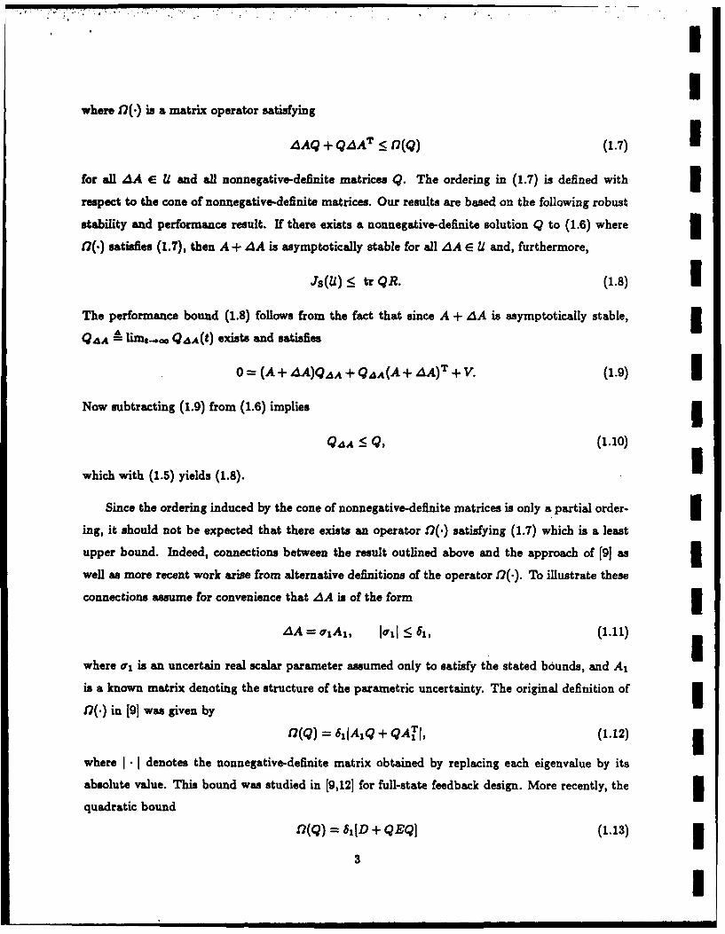
where D(.) is a matrix operator satisfying

AAQ + QAA T < n(Q) (1.7) 1for all AA E U and all nonnegative-definite matrices Q. The ordering in (1.7) is defined with

respect to the cone of nonnegative-definite matrices. Our results are based on the following robust

stability and performance result. If there exists a nonnegative-definite solution Q to (1.6) where 3t7(.) satisfies (1.7), then A + 4A is asymptotically stable for all AA E U and, furthermore,

Js(U) 5 tr QR. (1.8) 1The performance bound (1.8) follows from the fact that since A + AA is asymptotically stable, 3QAA liM--,o Q AA(t) exists and satisfies

0 = (A+ 4A)QAA + QAA(A+ AA)T + V. (1.9) 1Now subtracting (1.9) from (1.6) implies 3

QAA : Q, (1.10)

which with (1.5) yields (1.8). USince the ordering induced by the cone of nonnegative-definite matrices is only a partial order-

ing, it should not be expected that there exists an operator D(.) satisfying (1.7) which is a least

upper bound. Indeed, connections between the result outlined above and the approach of [9] as

well as more recent work arise from alternative definitions of the operator J7(.). To illustrate these

connections assume for convenience that dA is of the formAA -" oAl, Jail :_ 61, (.1

where a is an uncertain real scalar parameter assumed only to satisfy the stated bounds, and A,

is a known matrix denoting the structure of the parametric uncertainty. The original definition of

17(.) in [91 was given by

17(Q) = 611A1Q + QA1, (1.12) [

where I - denotes the nonnegative-definite matrix obtained by replacing each eigenvalue by its

absolute value. This bound was studied in [9,12] for full-state feedback design. More recently, the 3quadratic bound

n(Q) = 61 [D + QEQ] (1.13)

3 I

I.

has been considered, where D DIDI, E - EjTE 1 , and DI, E1 are a factorization of A1 of the3 form A1 = DIE. Bound (1.13) was studied in [29] for robustness analysis and in (17,25,28,30,33,36]

for robust controller synthesis. A third bound which has also been considered is the linear bound

m 12(Q) = 61[aQ + a- AiQAf ], (1.14)

3 where a is an arbitrary positive scalar. As shown in [331, bound (1.14) arises from a multiplicative

white noise model with exponential disturbance weighting. Control-design applications of bound

(1.14) are given in [23,27,33,34,35].

The principal contribution of the present paper is thus a unified development of bounds (1.12)-

(1.14) for both robust stability and performance analysis. In addition, we present a systematic

approach which pays careful attention to the structure of the uncertainty set U. For example, we3 show that bound (1.12) guarantees stability over a rectangular uncertainty set while (1.14) is most

naturally associated with an ellipsoidal region. Furthermore, to provide a methodical development,

we consider three classes of bounds (Type 1, I and III) which operate by exploiting, respectively,the symmetry of AAQ + QdAT, the structure of Q, and the structure of AA. This approach3 clarifies the relationships among different bounds and suggests several new bounds.

Finally, the present paper also considers an alternative functional for robust performance anal-

ysis. Specifically, in place of white noise disturbances, we reinterpret w(t) in (1.1) as a deterministic

L2 signal as in Ho theory ([6]). By imposing an L.. norm on the output Eoz(t), the corresponding

m performance measure is given by (see [38])

JD(U) = sup limsupA,.ms(QAA(t)R), (1.15)AAEU t--oo

in contrast to (1.5). Both performance measures Js(U) and JID() are considered in the paper.

The contents of the paper are as follows. After summarizing notation later in this section,3 the Robust Stability Problem, Stochastic Robust Performance Problem, and Deterministic Robust

Performance Problem are introduced in Section 2. In Section 3 the basic result guaranteeing robust

I stability and performance (Theorem 3.1) is stated. This result is easily stated and forms the basis for

all later developments. A dual version of Theorem 3.1 (Theorem 4.1) provides additional sufficient

conditions and clarifies connections to traditional robust stability results. The bound 17(.) and its

dual A(.) are given concrete forms in Section 5. In Section 6, the bounds of Section 5 are merged with

Theorem 3.1 to yield the main results guaranteeing robust stability and performance (Theorems

4l

I6.1-&5) via modified Lyapunov equations. In Section 7 we analyze the modified Lyapunov equations

with regard to existence, uniqueness, and monotonicity of solutions. Additional bounds are derived 3in Section 8 by utilizing a recursive substitution technique, while both upper and lower bounds are

obtained in Section 9. Finally, illustrative numerical examples are considered in Sections 10 and 311.

Notation INote: All matrices have real entries I

IR, IRrx#,IR, E real numbers, r x a real matrices, IRVxl, expectation

11 r x r identity matrix

asymptotically matrix with eigenvalues in open left half planestable matrix

S r r x r symmetric matrices 3IN' r x r symmetric nonnegative-definite matrices

IP? r x r symmetric positive-definite matrices IZ >Z2 Z1 - Z ,,, ZZ2 e S

Z1 > Z - Z2 IP, Z1,Z2 S Itr Z, ZT trace of Z, transpose of Z

Ai(Z) eigenvalue of matrix Z 1.X,.(Z) maximum eigenvalue of matrix Z having real spectrum

2. Robust Stability and Performance Problems

Let U c IR"' denote a set of perturbations AA of a given nominal dynamics matrix A E

W" . Throughout the paper it is assumed that A is asymptotically stable and that 0 E U. We

begin by considering the question of whether or not A+ 4A is asymptotically stable for all 4A E U.

Robust Stability Problem. Determine whether the linear system 3*(t) = (A+ 4A)z(t), t E [0, c), (2.1)

is asymptotically stable for all AA E U. I

To consider the problem of robust performance it is necessary to introduce external distur-

bances. In this paper we consider both stochastic and deterministic disturbance models. The 35

=m Nm m ros mmmml | ml| II /I

stochastic disturbance model involves white noise signals as in standard LQG theory while the de-3 terministic disturbance model involves L2 signals as in Hoo theory ([6]). By defining an appropriate

performance measure for each disturbance class it turns out that we can provide a simultaneous

3 treatment of both cases.

We first consider the case of stochastic disturbances. In this case the robust performance prob-

Snlem concerns the worst-case magnitude of the expected value of a quadratic form [Eoz(t)]T [Eoz(t)],

where the matrix E0 e ]Rqx' defines the output states, when the system is subjected to a standard3 white noise disturbance w(t) E 1R4 with weighting Do = W Id .

Stochastic Robust Performance Problem. For the disturbed linear system

*(t) = (A+ AA)x(t) + Dow(t), t E (0,oo), (2.2)

3where w(-) is a d-dimensional white noise signal with intensity Ij, determine a performance bound

6s satisfying

JRS(U) A sup iimsupIE [EO(t)]T[Eox(t)] } <5,S. (2.3)AAEU t--oc

3The system (2.2) may denote, for example, a control system in closed-loop configuration sub-

jected to external white noise disturbances for which z(t) A Eoz(t) may be the state regulation

3 error. Such specializations are not required for this development, however.

Of course, since Eo and Do may be rank deficient, there may be cases in which a finite perfor-3 mance bound Bs satisfying (2.3) exists while (2.1) is not asymptotically stable over U. In practice,

however, robust performance is mainly of interest when (2.1) is robustly stable. In this case the3 performance Js(U) is given in terms of the steady-state second moment of the state. The following

result from linear system theory will be useful. For convenience define the n x n nonnegative-definite

3matricesR ETEo, VA DoDo. (2.4)

I Lemma 2.1. Suppose (2.1) is asymptotically stable for all AA E U. Then

Js(U) = sup tr Q AAR, (2.5)AAEU

where n x n QAA A limt.. E [z(t)zT(t)] is given by

1 QAA = e(A+AA)tVe(A+ A A) T t dt, (2.6)

6

1

Iwhich is the unique, nonnegative-definite solution to

0= (A + dA)QIA + QdA(A + AA)T + V. (2.7) I

To state the Deterministic Robust Performance Problem some additional notation is required.

For a measurable function w : [0, oo) -- IRd define

II.,112 (f, WT(t)W(t)dt}* (2.8)1

Note that definition (2.8) is an L2 function norm with a Euclidean spatial norm. We now reconsider 3(2.2) with w(.) now interpreted as a square-integrable function. In this case the robust performance

problem concerns the worst-case Lmo norm of a quadratic form [Eoz(t)]T[Eoz(t)]. 3Deterministic Robust Performance Problem. For the disturbed linear system (2.2),

where 1w()l11 2 :_ 1, determine a performance bound PD satisfying 3JDo(U) -sp sup sup _E [o(t)] _D. (2.9)

AAEU l-(')112_I tW[0)

The following result is proved in [38].

Lemma 2.2. Suppose (2.1) is asymptotically stable for all AA e U. Then

JD(U) = sup AD.&(QAAR), (2.10) 3AAGU

where QAA is the unique, nonnegative-definite solution to (2.7). I

Remark 2.1. Although Js(U) and JD(4) arise from different mathematical settings they are

quite similar in form. Note that in general JD(U) _< Js(U), and JD(U) Js(U) if rank R = 1. 1Remark 2.2. In Lemma 2.2 QAA can be viewed as the controllability Gramian for the pair

(A + AdA, Do) rather than the state covariance. 1In the present paper our approach is to obtain robust stability as a consequence of sufficient

conditions for robust performance. Such conditions are developed in the following sections.

3. Sufficient Conditions for Robust Stability and Performance IThe key step in obtaining robust stability and performance is to bound the uncertain terms 3

AAQ + QAA T in the Lyapunov equation (2.7) by means of a function 12(Q). The nonnegative-

definite solution Q of this modified Lyapunov equation is then guaranteed to be an upper bound

7 I

for Q4A. The following easily proved result is fundamental and forms the basis for all later

developments. The hypothesis of this result are of a general nature and are not intended to be

directly verifiable. Suitably verifiable hypotheses are discussed later.

Theorem 3.1. Let £ : IN' -. IN' be such that

AAQ-+QAA T < 1(Q), AAE U, Q E IN n, (3.1)

and suppose there exists Q E IN' satisfying

I = AQ + QA T + f(Q) + V. (3.2)

I Then(A + AA, [V + f(Q) - (AQ + QAT] ) is stabilisable, ZiAE U, (3.3)

I if and only if

In this case, A + AA is asymptotically stable, AA E U. (3.4)

QAA5 _Q, AA EU, (3.5)

where QAA E INn is given by (2.7), and

I Js(U) trQ R, (3.8)

3 JD(U) <\max(QR). (3.7)

In addition, there exists AA E U such that (A+AA, [V+fCQ)- (AAQ+QzdAT)] ) is controllable

3 if and only if Q is positive definite. In this case (A + AA, [V + f(Q) - (4AQ + QAAT)] " ) is

controllable for all Z5A E U.

I Proof. We stress that in (3.1) 'Q" denotes an arbitrary element of IN" while Q in (3.2) denotes

a specific solution of the modified Lyapunov equation. This minor abuse of notation considerably

simplifies the presentation. Now note that for all zA E IRn x (3.2) is equivalent to

5 0 = (A + AA)Q + Q(A + ,A)T + (Q) - (AAQ + QAAT) + V. (3.8)

Hence, by assumption (3.8) has a solution Q E IN" for all AA E IR n x. If dAA is restricted to the set

U then by (3.1) 17(Q) - (dAq+Q,AT) is nonnegative definite. Now if the stabiizability condition

(3.3) holds for all AA E U, it follows from Lemma 12.2 of [39] that A+ AA is asymptotically stable

8

I

II

for all AA E U. Conversely, if A + AA is asymptotically stable for all 4A E U, then (3.3) holds.

Next, subtracting (2.7) from (3.8) yields 30 = (A + AA)(Q - QAA) + (Q - QAA)(A + AA)T + f(Q) - (,AQ + Qd AT), dA E U,

or, equivalently, (since A + AA is asymptotically stable for all 4iA E U)

q - QAA = j e(A+AA)[ f(Q) - ( dAQ + QAAT)]e(A+AA)?tdt > 0, AA EU,

which implies (3.5). The performance bound (3.6) is now an immediate consequence of (3.5). 3To prove (3.7) we note that it follows from Corollary 7.7.4 of [401 that if 0 < M, :_ M 2 then

A<.S(M 1 ) 5 A..(M2). Thus 1JD(U) = A..,I(QAAR) = A-.(EOQAAET) <A. (EQE T ) = ,X..(QR). (3.9)

Finally, it follows from (3.8) that the controllability condition holds for some AA E U if and only

if the Gramian Q is positive definite. Since Q is also the Gramian corresponding to A + zA for all 54A E U, then controllability holds for all 4A E U. 3

For convenience we shall say that fl(.) bounds U if (3.1) is satisfied. To apply Theorem 3.1, one 3first specifies a function n(.) and an uncertainty set U such that f(.) bounds U. If the existence of

a nonnegative-definite solution Q to (3.2) satisfying (3.3) or, equivalently, (3.4) can be determined 3analytically or numerically, then robust stability is guaranteed. One can then enlarge U, modify

f(-), and again attempt to solve (3.2). If, however, a nonnegative-definite solution to (3.2) cannot 5be determined, then U must be decreased in size until (3.2) is solvable. For example, 12(-) can be

replaced by en(.) to bound eU, where e > 1 enlarges U and c < 1 shrinks U. Of course, the actual 3range of uncertainty which can be bounded depends upon the nominal matrix A, the function f1(-),

and the structure of U. In Section 5 the uncertainty set U and bound fl(.) satisfying (3.1) are given

concrete forms. We complete this section with several observations.

Remark 3.1. In applying Theorem 3.1 it may be convenient to replace condition (3.3) with 3a stronger condition which is easier to verify in practice. Clearly, (3.3) is satisfied if V + f7(Q) -

(AAQ + Q4AT) is positive definite for all AA E U. This will be the case, for example, if either V 3is positive definite or strict inequality holds in (3.1). Also, it follows from Theorem 3.6 of [39] that

(3.3) is implied by the stronger condition 1(A + ,dA,Vi) is stabilizable, eA E U. (3.10)

9

I

ISimilar remarks apply to the controllability condition.

Remark 3.2. If only robust stability is of interest, then the noise intensity V need not have

physical significance. In this case one may either set V = e I,. where e > 0 is small to satisfy V > 0,

3 or set V = 0 and require that strict inequality hold in (3.1).

Remark 3.3. Since A is stable Q satisfying (3.2) is given by

Q = fo At [17(Q) + V]e Atdt, (3.1)

Uor, equivalently,Q = fo00At2(Q)eA"tdt + Qo, (3.12)

3where Q0 E IN" is defined by

Qo A j eAtVeA tdt (3.13)

and satisfies

0 = AQo + QoA T + V. (3.14)

Note that Q0 -- Q and that the nominal performances Js ({}) and JD ((0}) are given by tr QoR

3 and A,.(QoR), respectively.

Remark 3.4. Using (3.11) it is also useful to note that the bound for Js(U) given by (3.6)

can be written as

tr QR = tr eAt [(Q) + V]eAT'dtR = tr Po [f(Q) + V], (3.15)

where Po E IN' is defined byPa 4 o eA~tReAtdt (3.16)

J0

5 and satisfies

0= AT Po+PoA + R. .(3.17)

3 The bound tr Po [f(Q) + V] can be viewed as a dual formulation of the bound tr QR since the

roles of A and AT are reversed. Dual bounds are developed in the following section. Note that

3tr QoR = tr P0 V.

Remark 3.5. If D(.) bounds U then clearly 12(-) bounds the convex hull of U. Hence, only

Iconvex uncertainty sets U need be considered. Next, we shall later use the obvious fact that if 12'(-)

bounds U' and fl"(-) bounds U ", then n'(.) +f "(.) bounds U'+ U ". Hence if U can be decomposed

* 10

I

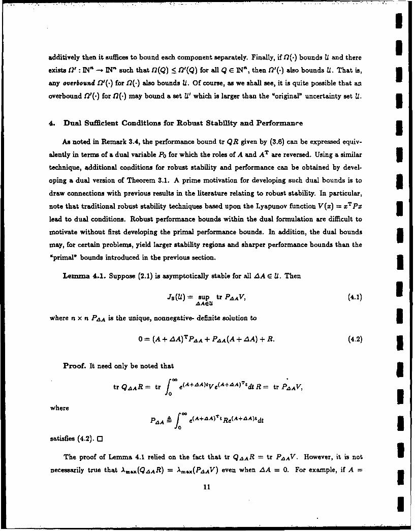
additively then it suffices to bound each component separately. Finally, if f7(-) bounds U and there

exists fT : IN' -- IN' such that f2(Q) ( 12'(Q) for all Q E IN-, then 17'(.) also bounds 1. That is, 3any overbound I(.) for 12(-) also bounds U. Of course, as we shall see, it is quite possible that an

overbound f2'(.) for n(.) may bound a set U' which is larger than the "original" uncertainty set U. 34. Dual Sufficient Conditions for Robust Stability and Performance 3

As noted in Remark 3.4, the performance bound tr QR given by (3.6) can be expressed equiv-

alently in terms of a dual variable P0 for which the roles of A and AT are reversed. Using a similar 3technique, additional conditions for robust stability and performance can be obtained by devel-

oping a dual version of Theorem 3.1. A prime motivation for developing such dual bounds is to 3draw connections with previous results in the literature relating to robust stability. In particular,

note that traditional robust stability techniques based upon the Lyapunov function V(z) - zTPz 3lead to dual conditions. Robust performance bounds within the dual formulation are difficult to

motivate without first developing the primal performance bounds. In addition, the dual bounds 5may, for certain problems, yield larger stability regions and sharper performance bounds than the

"primal" bounds introduced in the previous section. 5Lemma 4.1. Suppose (2.1) is asymptotically stable for all AA E U. Then

Js(U) = sup tr PAAV, (4.1)AAEU

where n x n PAA is the unique, nonnegative- definite solution to n

0 = (A + iA)TPAA + PAA(A + ZA) + R. (4.2) n

Proof. It need only be noted that I

tr QAAR = tr e(A+AA)tVe(A+AA)Ttdt R = tr PAAV,

where

PAA "A e(A+,A)Tt Re(A+AA)tdt

satisfies (4.2). [3

The proof of Lemma 4.1 relied on the fact that tr QAAR = tr PAAV. However, it is not I

necessarily true that Amax(QAAR) = Amx(PAAV) even when AA = 0. For example, if A =

11

nI

I

(2, 1n 113"" [ and thus A,.m (QoR)=3 ~ -[ 0 2] ,R=Ig,andV= []then QoR=[X I and PoV [X-2 1/3~1/4 [14"

(15 + -i4)/24 and A..,(PoV) = (5 + V' 7)/8. Thus to obtain a suitable dual version of JD(U)

we need to define a dual deterministic cost jD(U). This can be done if the disturbance signals are

taken to be integrable rather than square integrable. Thus, for measurable w : [0, oo) - IRd define

AI f'l 00- [WT' (t),WCt)] * dt, (4.3)

i which is an LI function norm with a Euclidean spatial norm. The dual deterministic cost jD(U) is

thus defined by

JD(U) A sup sup IIEx(-)II , (4.4)AAEU IIw(.)ll=<__j

where Ez(.) is measured according to the energy norm (2.8). The following dual result can also be

found in [38J.

3 Lemma 4.2. Suppose (2.1) is asymptotically stable for all AA E U. Then

i JD(U) = Amx(PAAV), (4.5)

where PAA is the unique, nonnegative-definite solution to (4.2).

IThe dual version of Theorem 3.1 can now be stated.

3Theorem 4.1. Let A: IN' --+ IN' be such that

IATp + PdA % A(P), A1A E U, P E IN", (4.6)

and suppose there exists P E IN' satisfying

0 = ATP + PA + A(P) + R. (4.7)

IThen([R + A(P) - (ZATP + PzAA)]*,A + ZA) is detectable, AA E U, (4.8)3 if and only if

A + AA is asymptotically stable, AA E U. (4.9)

5 In this case,

PAA _5 P, AAE U, (4.10)

l where PAA is given by (4.2), andJs (U) --< tr PVZ, (4.11)

12

I

I

ID(U) _ A,.,(PV). (4.12)

In addition, there existsdLAr: U such that ([R+ A(P) -(AATp+ PAA)]2L,A+ AA) is observable3

if and only if P is positive definite. In this case ([R + A(P) - (,dATp + PA)] *, A + 4A) is

observable for all AA EU. 3Proof. The proof is completely analogous to the proof of Theorem 3.1. 0

Remark 4.1. Note that JD(U) Js(U) and .D(U) = Js(U) if rank V = 1. Combining this

fact with Remark 2.1, it follows that JDD(U) = JD(U) if both rank R = 1 and rank V = 1. 1

It is quite possible that the bounds tr QR and tr PV for Js(U) given by (3.6) and (4.11) may

be different in spite of the fact as shown in the proof of Lemma 4.1 that tr QAAR = tr PAAV. 3That is, depending upon 12(.) and A(.) either bound (3.6) or bound (4.11) may be better for a

particular problem. In general, we have the following result. 3Proposition 4.1. Let n(-),A(.),Q, and P be as in Theorems 3.1 and 4.1, and let Q0 and P0

be given by (3.13) and (3.16), respectively. Then Itr QoA(P) < tr Po(Q) 4=* tr QR > tr PV, (4.13) 3tr QoA(P) = tr PoF(Q) 4=* trQ R = tr PV, (4.14)

tr QoA(P) > tr Po0(Q) -= tr QR < tr PV. (4.15) 3Proof. Note that 3

tr QR = j eAt P(Q) + V]eA tdt R = tr PoI7(Q) + tr j eAtVeA T tdt R

and

tr PV = tr j eA T [A(P)+R]eAtdtV = trQoA(P)+ tr j eATtReAtdtV

so that

tr QR- tr PV = tr Po2(Q) - tr QoA(P), 3which yields (4.13)-(4.15). 0

Remark 4.2. Finally, as shown by example above, it is not generally true that JD(U) = JD(U).

Similarly, we should not expect that the bounds Am.(QR) and Am.x(PV) for JD(U) and JD(U) 3given by (3.7) and (4.12) are equal.

13

I

I

5. Construction of the Bounds tl(.) and A(.)

3 As discussed in Section 1, we consider three distinct classes of bounds t2(-) denoted by Type I,

Type U, and Type III. Roughly speaking, these bounds exploit, respectively, the symmetry of the

m Lyapunov terms dAQ + QAAT, the structure of Q, and the structure of A1A. The dual bounds

A(-) can be constructed similarly by replacing Q and AA by P and Z1AT. Hence these bounds

will not be discussed separately. For convenience in discussing the set U, we shall use the terms

rectangle and ellipse to refer to closed regions bounded by such figures in multiple dimensions. As3 usual, a polytope is the convex hull of a finite number of points.

5.1 Type I Bounds

We begin by constructing bounds D(.) which exploit only the symmetry of the Lyapunov terms3 4 AQ + QAAT. First we require the following definition of a function of a symmetric matrix as an

extension of a real-valued function ([40], p. 300). Specifically, if f: IR --I R then (with a minor3 abuse of notation) f: S" -+ S" can be defined by setting

I(S) A Uf (D) UT,

m where S = UDUT, U is orthogonal, D is real diagonal, and f(D) is the diagonal matrix obtained

by applying f to each diagonal element of D. Note that if . is the polynomial f(z) = E=0 aix'

then f(S) = ,__0 a.S. Note also that if f(z) = fzj then f(S) = (SI)i, where (.)i denotes the

(unique) nonnegative-definite square root. As in [41], p. 262, we use the notation ISI to denote3 (S2) 1. Finally, note that if f: IR --I R and g: IR -- IR are such that f(z) _ g(z), z E IR, thenf (S) :_ g(s), S ES".

I As a concretization of the uncertainty set U, consider the set

pI" Zi A {dA EIR'nn: dA =Fao'A., jaoi ]_<6,, i =1,...,p), (5.1)

i=1

m . vhere, for i = 1,... ,p : A. E WRfx' is a given matrix denoting the structure of the parametric

uncertainty; or is a real uncertain parameter; and 6i denotes the range of parameter uncertainty.

Clearly, the multidimensional set of uncertain parameters (oru,... ,op) is the rectangle [-81, 811 x

... × [-6p,6p] and U1 is a symmetric polytope of matrices in lR"'". Note that the symmetry of

the uncertainty interval [-6,,6,] entails no loss of generality since the nominal value of A can be

redefined if necessary. Furthermore, it is also possible, without loss of generality, to define i = 1by replacing A. by 6A. For clarity, however, we choose not to employ this scaling.

14

U

I

We begin by considering the absolute-value bound utilized by Chang and Peng in [9].

Proposition 5.1. The function NP

n,(Q lA8iQ + QAT 1 (5.2)s=1

bounds UI.

Proof. For i = 1,...,p and Il5 Si<,,

-,(AQ + QAT) _ I,(AQ + QAT)I = iojlA.Q +QATI <5 $,IAQ + QAZI. IThus, summing over i yields

P P

AAQ + QdAT = u,(A.Q + QAT) < _ Z ,IA.Q + QATI,i= =1U

which yields (3.1) with n(.) = nl1 () and U = U1. 0

Remark 5.1. It is tempting to prove Proposition 5.1 by writing 1P P P

Z ,('AQ + QZ) :_ I Z i(,( Q + Q4)I -ZI(AQ + QAT)I. 3However, counterexamples show that the inequality IM1 + MI IMI + I M21 is not generally true

for arbitrary symmetric matrices M, M2 .

Remark 5.2. Because of its simplicity it is tempting to conjecture that 171(') is the best bound

for 4AQ + QAAT over the set U1. To show that this is not the case, let Q = .12, p = 1, A1

[-1, and 61 = 1. Then o'(AIQ +QAT) :5 61 jA 1Q +QATI =2,1o'11 :5 1. However, it is also

true that o, (AzQ + QA) [12s/22 ] Jai o < 1. Neither bound, however, is an overbound for

the other. This is a consequence of the fact that the nonnegative-definite matrix ordering is only a

partial order.

As mentioned above, an overbound for f12(') will also bound U1. 3Lemma 5a. For i 1,...,p, let f,: IR -- IRsatisfy

fi(x) I1, E IR. (5.3)

Then the function ID2(Q) i f ,,(AQ + QA,) (5.4)

1I

15 I

. . ... . . . ,.. .. .

I

is an overbound for nL1 (.) and hence also bounds U1.

3 One particular choice of f/ satisfying (5.3) will be considered here, namely, the polynomial

i / 4(f) i ,6 -'x, (5.5)

where fl is an arbitrary positive constant. Thus 172(.) has the following specialization.

U Coroliary 5.1. Let, ..... ,6p be arbitrary positive constants. Then the function

P Pfs(Q) A . 6,#, . + Z(Q/)(,,q + Q,7)2 (5.6)I --1 .1

3 is an" overbound for 171 (') and hence also bounds U1.

Although overbounding fl1 (') by f2s(-) results in a looser bound for U1 , it turns out that fs(-)3 actually bounds a set which is larger than U1. Specifically, in place of U, consider

P p

U2 AA E IZ < 1}, (5.7)I---_where a p,...,a, are given positive constants. Note that (5.7) replaces the rectangle of uncertain3 parameters (..,.-. ,up) by an ellipse. Thus the set U2 of matrix perturbations is an ellipse of

matrices in IR x"' in contrast to the polytope U1. Of course, U! = U2 if p = 1 and aj = 61. Again3 it is possible to take aj = 1 without loss of generality by replacing A. by a Aj. We again choose not

to do this, however. The following lemma provides a convenient characterization of the relationship3 between the rectangle U1 and the ellipse U2 .

Proposition 5.2. Suppose U1 is defined by the positive constants 61,...,6p and let U2 be

I characterized by

I where a is defined by

p

and 61,... , are arbitrary positive constants. Then U2 contains U1 . Specifically, the ellipse U23 circumscribes the polytope U1. Furthermore, f23(.) actually bounds Z 2.

Proof. If Ja -: 6,, i = 1,... ,p, then it follows from (5.8) that

p P p

I t=1 i-.-1 i=

16

I

II

If, in addition, Iai = l , i 1,... ,p, then F,X 6 =/a; 1, which corresponds to a point on the

boundary of the ellipse. To show that f23(.) actually bounds U2 note that

Po _ [1(o4aj._ , /c,. , - (,o,/o*)(A,. + QA)]i

p p4 E(j(o/o,;)I,. + a, . o(A.Q + QA!') _ (AAQ + QAA T ).

Since r2/a < 1 in U2 , it follows that

AAQ +QA T < IR+a,1 Aq+qAT)2.

Utilizing (5.8) and (5.9) to substitute for a and aj yields (3.1) with 12(.) = l2(.) and U = U2. 0

Proposition 5.2 shows that each choice of constants 1 ..... Op > 0 leads to a particular ellipse IU2 which contains the polytope U1. Furthermore, 173(-), which by Corollary 5.1 bounds U1, actually

bounds the larger set U2 . For convenience, we now dispense with the constants ...... ,6,p which mrelate the rectangle U1 to the ellipse U2 and we characterize 173(.) entirely in terms of a p,..., a.

Corollary 5.2. Let a be an arbitrary positive constant. Then the function

74 (Q) -'2L2 ., + C'a;1 Xk(A.Q + QAI) 2 (5.10)1

bounds U2.

Remark 5.3. Within the context of Corollary 5.2, the positive constant a plays no role in

defining the set U2 , although f24 (') is guaranteed to bound U2 for all choices of a. It can be

expected, however, that certain choices of a provide better bounds than other choices. This will

be seen by example in Section 10.

5.2 Type H Bounds

We now consider additional bounds for U which exploit the structure of Q. For these bounds

the natural uncertainty set is given by U2.

Proposition 5.3. Let a be an arbitrary positive number and, for each Q E IN', let Q, E 3IR"x ' and Q 2 . lR" xn satisfy

o 1 2 . (5.1) m

17

I I

Then the functionP525(Q) A aQq +kA.Q 1 QTAT (5.12)

bounds U2.

Proof. Note that

U 0 < r [(ag,/,)QT (Ct,/Ck4)A.Q1] [(a4ff,/a,)QT _-C )A ]

I = p Pp

Cg (0,/Cg)QT'Q + a gaA.iQzQ1'AT - Z ,(A..Q + Q4),i---1 1=1 1

which, since E? r/a < 1, yields (3.1) with 7(.) = s(.) and U = U2. 13

We consider three specializations of [25 (-). Specifically, we set m = n and define

Q1 = Q, Q2 = ,1 , (5.13)

Q1 = Q2 = Qi, (5.14)

5 Q1 = I., Q2 = Q. (5.15)

3 Corollary 5.3. Let a be an arbitrary positive number. Then the functionsp

nte(Q) A c +a -- % ,.A2AT, (5.16)

?7(Q) A I, + a E aA. A, (5.17)I p-.

178(Q) A CkQ2 + CII ZaA.A" 5.8

bound U2.

m Remark 5.3. Note that the term AiQ 2 AT appearing in fl(.) also appears in nl4('). Further-

more, both r24(-) and fls(.) involve a term proportional to I.. Despite these similarities, neither3 bound n4(') nor ns() is an overbound for the other.

Remark 5.4. The bound 127(') given by (5.17) has the distinction that it is linear in Q. This

bound was originally studied in [23,27] for systems with multiplicative white noise and was shown

to yield robust stability and performance in [33,35]. A similar bound was studied in [34].

18

m

I

Remark 5.5. Using (5.11) additional bounds can be developed. For example, by setting

Q, = Q, Q2 = Q, (5.19) 3hl(Q) becomes IDq(Q) = C1Qi + a-' cO Q AT ,. (5.20)

Remark 5.6. When p = 1 and a is replaced by aa, 17 (.) becomes I17 =4l~Q(Q) = ixq+cA iQAI

Utilizing a sum of such terms with ai = 6 can be used to bound the smaller rectanguh., set U1.

Similar remarks apply to t76('), 17s('), and 17g(-).

5.3 Type M11 Bounds 3We now consider bounds which exploit the structure of dA itself. It turns out that these

bounds permit consideration of an uncertainty set U which is larger than U2. Specifically, define 3U3 A { AA IR x' : AA.:- MN, MMT < D, NTNS <E}, (5.21) 3

where M E IR x"'t and N E IR"x " are uncertain matrices, r is an arbitrary positive integer, and

D, E E IN" are given uncertainty bounds. The bound f210(') for Us is given by the following result. 3Proposition 5.4. Let a be an arbitrary positive constant. Then the function

= a- D + aQEQ (5.22)

bounds Us. IProof. Note that 3

0 <_ [&i-M - aIQNT][,--M - ,IQNT]T'

CkalMMr + o:QNTNQ - [MNQ + Q(MN)T]

<a-D + aQEQ - (,AQ + QdAT),

which yields (3.1) with ft2(-) = 12,o(-) and U = U3. 0 3Remark 5.7. The bound f710(') was developed independently in [291 for robust analysis and in

[25,281 for robust full-state feedback. Applications to fixed-order dynamic compensation are given

in [36].

19

I

m

Remark 5.8. Without loss of generality we can set a = 1 in (5.22) by replacing D and E by5 c- 1D and aE, respectively. Again for clarity we have chosen not to employ this normalization.

Note that f1 0 (') is an overbound for fls(') when D and E are chosen to satisfy

I _!Ai < D, .< E. (5.23)

3 Hence, in this case 1210(') necessarily bounds U2 . As in the case of 173 (') overbounding fDl('), we

should not be surprised to find that fl1 0 (') actually bounds a set larger than U2 . Indeed, we now

show that U2 is actually a very special subset of Us when D and E defining U2 satisfy (5.23).

Proposition 5.5. Suppose D and E satisfy (5.23). Then U2 is a subset of Us and thus the

3 bound f 10 (.) for Us also bounds U 2.

Proof. If AA E U2 then AA = F,? , where ? u2/a < 1. Alternatively, we can

write AA = MN, where r = pn and

M =(iA...mapA,], N- : (5.24)

Note that with D and E satisfying (5.23) and M and N defined by (5.24) it follows that MMT <- D

and NTN < E. Thus dA E Us. [3

The following result provides general conditions under which f11 0 (.) bounds U2 .

Proposition 5.6. Suppose A. = DE, i = 1,...,p, where Di E IR"'" and E E IRlX '

m and suppose that P P

ceDi DT < D, ijEE, :_ E. (5.25)I $ =1fi

Then U2 is a subset of U3 and thus the bound 1710 (.) for U3 also bounds U2.

5 Proof. The result follows as in the proof Proposition 5.5. []

Remark 5.9. When p = 1, D - '2DIDT and E = ETE, it is convenient to replace ct by

I mi so that f11 0 (') becomes

3 no(Q) = cti[a-DID + aQE E1Q]. (5.26)

In certain situations it is desirable to consider subsets of U3 of special structure. For example,

m define

U4 -A {AA E IR " " : AA = DoMNEo, DoMMT D T < D, EJoNTNEo _ E},

20

I

where Do E lR x ft l and E0 E IRnS xn are known matrices denoting the structure of the uncertainty,

and M E IRF ' Xr and N E IRrXft2 are uncertain matrices. Finer structure can be included within

U4 by replacing DoMNEo by a sum of terms DMiNiEi, where Di, E, are known and M,, N are

uncertain ([291). Note, however, that even though U4 is a proper subset of Us, the form of the 5bound Dl 0 (') does not change. Thus such refinements render the bound r2o(') conservative with

respect to U4 since the larger uncertainty set U3 is actually being bounded. 36. Robust Stability and Performance via Modified Lyapunov Equations 3

We now combine the principal results of Sections 3, 4 and 5 to obtain a series of conditions

guaranteeing robust stability and performance. In particular, we focus on bounds 121,174 ,[26, 7l7 ,

and [10. For simplicity we shall frequently assume that V is positive definite so that (3.3) is

satisfied. In this case it follows that the solution Q of (3.2) is positive definite. Our first result is a icorollary of Theorem 3.1 with 17(-) = 17,(.) and U = U.

Theorem 6.1. Let V E IP", 61,...,Sp > 0, and suppose there exists Q E IP" satisfying I

o=AQ + QA T + Z _iIQ + QATI + V. (MLE1)

Then A + AA is asymptotically stable for all AA E U1, and 5Js(Ul) 5 tr QR, (6.1)

JD(Ul) 5 A..( R). (6.2) IFor the next result define

A. A A+ sr. (6.3)

and

, ... 1P. (6.4)

Setting 17(-) = 174 (.), DO(.),f17(.) and U U2 yields the following corollary of Theorem 3.1. 3Theorem 6.2. Let V E IPf, a, al,... ,ap > 0, and suppose there exists Q E IP" satisfying

either 30= A Q Q AT + ' (AjQ + QAT)2 + %I,. +V, (MLE2)

21

I

Io= AQ + QAT + ZyiAQ'A! + ciI + V, (MLE3)I s---1

orP

0= AQ + QAT + Z-i A.QA7 + V. (MLE4)

Then A+ AA is asymptotically stable for all AA E U2, and

I Js(U2) - tr QR, (6.5)

I JD(U 2) < \..(qR). (6.6)

3 Next we set 12(-) = l10 (') and U = Us.

Theorem 6.3. Let V E IPID E IN', and E E IN", and suppose there exists Q e IP"

3 satisfying

0 = AQ + QA T + cQEQ + a-'D + V. (MLE5)

I Then A + AA is asymptotically stable for all AA e U3 , and

Js(Us) _ tr QR, (6.7)

J'D(U3) < \..(QR). (6.8)

Additional sufficient conditions can be obtained by considering "mixed" bounds. That is, one

can construct modified Lyapunov equations by combining two or more different bounds. Although

mixed bounds will not be considered further in this paper, we present onc o.,.h result for illustrative

purposes.

3 Theorem 6.4. Let V E IP ,,... ,6p > 0, D E INn, and E E IN", and suppose there exists

Q E IP' satisfying!P0 = Aq + qAT + 5,jA,q+QA!'j+ QEQ+ a-'D+V. (MLE1, 5)

i= 1

3 Then A + AA is asymptotically stable for all AA E U, + Us, and

3 Js(U1 +U3) 5 trQR, (6.9)

JD(Uj + Us) : Aax(QR). (6.10)

* 22I

IAs noted previously, the bound A(.) can readily be constructed by replacing AA by dAT in the

definitions of O7I(.) through 7lo('). Denote these bounds by A,(.) through A10(.), respectively. For

illustration we state the dual of Theorem 6.1 involving A,(.). The dual versions of MLE1 through

MLE5 will be denoted by MLEDI through MLED5.

Theorem 6.5. Let R E IP', $1, ... , 6p > 0 and suppose there exists P E IP h satisfying

0= ATp +PA + ZSIATP + PA.1 + R. (MLEDI)

Then A + AA is asymptotically stable for all AA E 3 , and

Js(U1) :5 tr PV, (6.11) .

JD(UL) <5 -X..(PV). (6.12)

It is reasonable to expect that the sufficient conditions given by Theorems 3.1 and 4.1 are

generally different. For example, the modified Lyapunov equations and their duals need not both

possess a solution, while the bounds tr QR and tr PV need not be equal. An exception is the case

in which 17(.) = 177(.) and A(.) = A7(.). Note that the dual of MLE4 is given by

0= AP + PA. + > y4' APA. + V. (MLED4)

Proposition 6.1. Let a,, ... , cp > 0 and assume there exist Q, P E IN" satisfying MLE4 and

MLED4, respectively. Then =tr QR =tr PV. (6.13)

Proof. Note that Itr QR = -tr Q(AP + PA. + > yi/ATPA.) 3

--tr P(A.Q + QAj + EyiAQA") 3= tr PV. 0

Remark 6.1. By setting f7(.) = 177(.) and A(.) = A7(.) it follows from (4.14) that Ip p

tr Qo(aP+ E iATPAi) = tr Po(o:Q + Z-j,A,QAT). (6.14) 3i=11

23 I

I7. Existence, Uniqueness, and Monotonicity of Solutions to the Modified Lyapunov

Equations

It is important to stress that the sufficient conditions for robustness given by Theorems 6.1-6.5

assume only that there exist nonnegative-definite solutions Q, P satisfying the modified Lyapunov

equations. Indeed, no explicit assumptions on the problem data A,V, R, and U were utilized for

assuring robust stability and performance. In applying Theorems 6.1-6.5 to specific problems it thus

suffices to show that a nonnegative-definite solution Q exists in order to obtain robust stability,

while, for robust performance, the bounds (6.1), (6.2), (6.5)-(6.8) require explicit knowledge of

Q. Thus, any computational method which yields a nonnegative-definite solution will suffice to

guarantee both robust stability and performance.

Before considering the numerical solution of the modified Lyapunov equations, several relevant

Iissues require discussion. For example, before seeking to compute solutions to MLE1-MLE5 it

would be desirable to determine a priori whether these equations actually possess nonnegative-

definite solutions. For example, it may be useful to obtain sufficient and/or necessary conditions

for the existence of nonnegative-definite solutions. Thus, if the sufficient conditions are satisfied

then existence (and hence robustness) is assured, while if the necessary conditions are not satisfied

then existence is ruled out. If, on the other hand, either the sufficient conditions are not satisfied or

the necessary conditions are satisfied, then nothing can be surmised. Finally, such conditions need

to be easily verifiable and reasonably nonconservative since otherwise it would be more prudent to3attempt to numerically solve the modified Lyapunov equation itself.

It is quite possible that at least some of the modified Lyapunov equations possess multiple5nonnegative-definite solutions. In this case one may seek the minimal solution (i.e., the smallest

with respect to the nonnegative-definite matrix ordering) in order to minimize the performanceUbounds. If multiple solutions exist, none of which is minimal, then the best bound would depend

upon the matrix R.

5Since the matrix Q determines the performance bound, it is reasonable to expect that Q is

monotonic in U. That is, if U decreases in size, then the solution Q is more likely to exist while5decreasing in the nonnegative-definite matrix ordering. For example, consider U characterized by

5j, where 8 < 8, i = 1,... ,p. Then one might expect Q' < Q where Q' is the solution to MLE15with 6 replaced by 8. Finally, monotonicity with respect to V should also be expected.

I 24

I

I

Because of linearity, the analysis of bound 1 7 (-) is simplest and it is possible to obtain necessary 1and sufficient conditions for the existence of solutions to MLE4. The basic tool required is the

Kronecker matrix algebra ([42]). For convenience, define

A aA. Q a. -+ yAi A.. (7.1)

Proposition 7.1. If V E IN' and A is asymptotically stable, then there exists a unique n x n Q Isatisfying MLE4, and Q > 0. Conversely, if for all V E IN' there exists Q 0 satisfying MLE4,

then A is asymptotically stable.

Proof. Since MLE4 is equivalent to

q = -vec 1 [A'vec V], (7.2)

existence and uniqueness hold. Here, vec and vec -1 denote the column-stacking operation ([42])

and its inverse. To prove that Q is nonnegative definite, we rewrite (7.2) as

Q = o vec-[eAtvec V]dt (7.3)

and show that the integrand is nonnegative-definite for all t E [0,oo). [Note that the following

argument does not require that A be stable.] Using the exponential product formula, the exponential 3in (7.3) can be written as

eAt-=im { exp [j(Aa e A.)t] exp [f ,:-tr(Ai ® Ai)t] } (7.4). k~a f ki=1

For convenience, let S and N be r x r matrices with N > 0. Since (see [42]) Ivec- 1 [(S 0 S)vec N] = SNST 0 (7.5) 3

and(S; ® Sk)(S & S) = Sk+I ® sk+I,

(7.6)

it follows that3 I

vec-'[eS®Svec NJ = Z(k!)-S"NSkT > 0. (7.7)

Furthermore, 3vec '[eSSvec N] = vec-[(es 9 es)vec N] = eSNesr > 0. (7.8)

25

U

I

U Applying (7.7) and (7.8) alternately with (7.4).and using induction on k it follows that the integrand

of (7.3) is nonnegative definite. To prove the converse, note that it follows from MLE4 that Q

satisfies

Q = vec-I[e-"vec Q] + J vec- 1 [e"'vec V]ds, t E [O,oo). (7.9)

Since the integral term on the right hand side of (7.9) is nonnegative definite, is bounded from

above by Q, and V E IN' is arbitrary, it follows that A is asymptotically stable. 0

We now show that if A is asymptotically stable then actually Aa is asymptotically stable. This3 shows that the assumption that A is asymptotically stable is consistent with the original hypothesis

that A is asymptotically stable.

Proposition 7.2. Assume A is asymptotically stable, let a E [0, ], i ... ,p, and define

Then A' is also asymptotically stable. In particular, A. and A are asymptotically stable.

Proof. Let V E IN' and let Q be the unique, nonnegative-definite solution of MLE4. Equiva-

lently, Q satisfiesp

O= AaQ+QA, E+ (a /ct)AQAT +V',

j=1where

! ±wher -"- A -'(cr -,,c')A.QA, + V.

Since V' E IN', the stability of A' now follows from the converse of Proposition 7.1. Finally, if

'IP then f /)AjQA + V' is positive definite and it follows from Lemma 12.2 of [39]3 that A., and hence A, is asymptotically stable. 0

Hence it follows from Proposition 7.2 that a necessary condition for A to be asymptotically

sstable is that

a < 2 max Re A,(A). (7.10)3 ...,n

We now have the following monotonicity result.

Proposition 7.3. Let UI C U2 , where U is defined as in (5.7) with a, replaced by a E

[0, oj, i = 1,... ,p. Furthermore, let V E IPn , assume A is asymptotically stable, and let Q E INn

I26

satisfy MLE4. Then there exists Q' E IN^ satisfying IST + IQA +V

0= A.Q'+ Q'AI + 2(o /c)AQ'AT + V2 (7.11)

and, furthermore, IQ' < Q.(7.12)

Consequently, I

tr QIR5 _tr QR, (7.13)

A=.(Q'R) <_ -m..(QR). (7.14)

Proof. Subtracting (7.11) from MLE4 yields I

0 = A,.(Q - Q') + (Q - Q')Al + ( o:'/ )A, (Q - Q')AT + V',

where V' is defined in the proof of Proposition 7.2. Since, by the converse of Proposition 7.1, A' is

asymptotically stable, Q - Q' >- 0, which yields (7.12) and thus (7.13) and (7.14). 0

Returning now to the existence question, Proposition 7.1 shows that a solution to MLE4 exists Iso long as a, ... ap are sufficiently small that A remains stable for some a > 0. To this end one

can treat this as a stability perturbation problem and apply resultsfrom [3]. Within our modified

Lyapunov equation approach we have the following related result. For this and the following result

let 1I -1 denote an arbitrary vector norm and the corresponding induced matrix norm.

Proposition 7.4. If 3II(A9A)-(aI.2 +&-1 a!A®A,)II < 1, (7.15)

then for all V E IN' there exists Q e IN' satisfying MLE4 and hence A is asymptotically stable.

Proof. Define {Qk)'Zo where Qo satisfies (3.14) and Qk+j satisfies I

0 = AQk+j + Qk+IA T + f27(QA) + V. I

Note that Qh 1_ 0, k = 1,2, .. Hence it follows that 3vec Q5+1 - vec Qk = -(A B A) - [vec fl,(Qk) - vec fl(Qkl)]I

27

I I

I,

I and thus

pIlvec Qv+1 - vec QhII 5 II(A 9 A)-'(arI.2 + acI Zc2A. 0 Ai)IIIlvec Qk -vec Qk-11I.

i=1

Using (7.15) it follows that Q A im-.00 Q; exists. Thus Q 2 0 and satisfies MLE4. Finally, by

the converse of Proposition 7.1, A is asymptotically stable. 0

I Since MLE5 is nonlinear a slightly different approach is required for existence. For the following

result let , > 0 satisfy ieA 111 <_ ke - ', t _> 0, (7. 6)

3 where 11 f1 denotes an arbitrary submultiplicative matrix norm, and define p a 2,/8/1.

Proposition 7.5. Suppose V e IN' and

4ah IEll II,-'D + Vii < P2. (7.17)

Then there exists Q E IN" satisfying MLE5.

Proof. Consider the sequence {Qk}ffo where Q0 satisfies (3.14) and Qk+i is given by

0 = AQk+lT Q+AT+ AEQk + o-lD + V.

Clearly, Qk _ 0, k = 0, . Next we have

IQk+ =10 CAICxQkEQk +cz'D + V~c.Ar *dt (7.18)

Iwhich yields" " -. Ill <- p-IIEIIIIQkII2 + p-1 Ii - 1D + VII. (7.19)

3Similarly, we obtain

IIQoll -< p'll-'D + VII.

INow suppose that

Then (7.17) and (7.19) imply

IIQ.+1ll -5 oSp-illEI [2p-lla - D + VII] 2 + p-llo- D + Vii< 2p- 'lI0-:1D + V II.

I

I

Thus IIll _5 2p- 111a- 1 D + Vi, k= 0,1 . Next, (7.18) yields

Qk+1 - Q.= a f 0 eAt[qh.Eqh. _ Qh._EQk...L]CArtdt

= af eAt [QhE(QA: - Qk-iL) + (Qk - Qk-l)EQ-._.]CATtdt

IIQk+l - QA;i- W-p1 E11E(IIsII + IIQi-iII)IIQA; - Qk-II

-4ap-2 IIEIJI-'D + VIIIIQI - Qk-I 11

-'IIQ - QI.+III,where e A 4ap 211EII1la-1 D+VI. Since by (7.16) e < 1, limi,.. QA; exists, is nonnegative definite,

and satisfies MLE5. [

8. Additional Upper Bounds via Recursive Substitution

In this section we obtain additional upper bounds for Js(U) and JD (U) by utilizing a recursive 1substitution technique. The main idea involves rewriting (2.7) as

QA = -vec- {(A e A)-(AAe AA) vec QAA} + qO (8.1)

and substituting this expression into the terms AAQ.AA + QdAAAT appearing in (2.7). This

technique yields an equation which is, as expected, equivalent to (2.7) but which permits the

development of additional bounds. As will be seen, the ability to develop new bounds exploits

the fact that the substitution technique leads to terms which are quadratic in AA. We begin the

development with the following technical result which does not require the assumption that A is

asymptotically stable.

Proposition 8.1. Suppose A 9 A is invertible and let A A E IR " x'. If QAA satisfies (2.7)

then QAA also satisfies

O= AQ'A + QAAAT- vec-1 [(A g A A)(A9 A)-(AA @' A)vecQA (8.2)1

+ (AA 9 AA)(A e A)- 1 vec V] + V.Conversely, if QAA satisfies (8.2) and (A - AA) e (A - ,A) is invertible, then Qe',A also satisfies

(2.7).

Proof. To obtain (8.2) substitute (8.1) into (2.7) as noted above. Conversely, adding the zero

term (,dA e ,A)(A 9 A)-l(A GD A)vec QAA - (AA e AA)vec QAA to (8.2), it follows that (8.2)can be written as 3

0 = [(A- AA) 9 (A- AA)](A 9 A)-[(A + AA)G (A + AA)vec QAA + vec V],

29

i which, under the invertibility assumption, implies that QAA satisfies (2.7). 03

The following result is analogous to Theorem 3.1.

Theorem 8.1. Suppose U is symmetric, let Do E IN' satisfy

AAQ 0 + QoAA T < 1 0 , AA E U, (8.3)

i where Qo satisfies (3.14), let : IN' --+ IN' satisfy

3 -vec-[(A AA)(A 9A)-(AAeAA)vecQ] 56(Q), dAEU, QEIN", (8.4)

and suppose there exists Q E IN^ satisfying

0 = AQ + QA T + f(Q) + 2o + V. (8.5)

Then

(A + AA, {fl(Q) + vec-" [(AA eD AA)(A 9 A)-1 (AA E AA)vec Q] + 12o +V}*) (8.6)

is stabilizable, AA E U,

i A + AA is asymptotically stable, AA E U. (8.7)

In this case,

3 QA_ Q, AA E U, (8.8)

where QAA satisfies (2.7), and

Js(U) 5 tr QR, (8.9)

JD(U) 5 Amax(QR). (8.10)

Proof. The equivalence of (8.6) and (8.7) follows from (8.5) as in the proof of Theorem 3.1.

Next (8.8) follows by comparing (8.5) and (8.2) while using (8.3) and (8.4). Since U is assumed to be

symmetric, it follows that A-AA is asymptotically stable, AA E U, and hence (A-AA)e (A-AA)3 is invertible, AA E U. Thus, the converse of Proposition 8.1 implies that QAA satisfying (8.2) also

satisfies (2.7). Thus, the bound (8.8) can be used to obtain (8.9) and (8.10). 0

3 The principal difference between (8.4) and (3.1) is that dA appears linearly in (3.1) while it

appears quadratically in (8.4). By exploiting this structure we can obtain new bounds for QAA.

* 30I

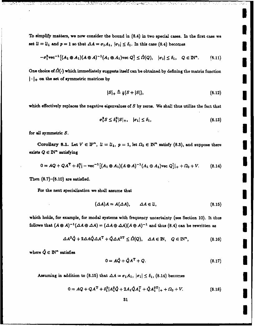
II

To simplify matters, we now consider the bound in (8.4) in two special cases. In the first case we

set U = and p = I so that AA = a1 A 1, uall 5 81. In this case (8.4) becomes

- 1vec1 [(A, 6 Ai)(A 9 A)-(A,, AI)vec Q] :_ 6(Q), 1ar, <_a,, Q E IN'. (8.11) IOne choice of 6(-) which immediately suggests itself can be obtained by defining the matrix function

I -1+ on the set of symmetric matrices by

IS1+ i (s + ISI), (8.12)

which effectively replaces the negative eigenvalues of S by zeros. We shall thus utilize the fact that

als _ 6lsl+, Iu1 -< 6 , (8.13)

for all symmetric S. ICorollary 8.1. Let V e IP", U = U1, p = 1, let 1o E IN' satisfy (8.3), and suppose there

exists Q E WN" satisfying

0=AQ + QAT + 621 -vec[(A 1 GAl)(AG A)-(A 1 E@AI)vecQ]I++ o+V. (8.14) IThen (8.7)-(8.10) are satisfied.

For the next specialization we shall assume that

(AA)A = A(AA), A A E U, (8.15)

which holds, for example, for modal systems with frequency uncertainty (see Section 10). It thus

follows that (A9 A)-'(AA G AA) = (AA( AA)(A $ A)- 1 and thus (8.4) can be rewritten as

AA 2Q + 2AAAA T + QAA2T < f(q), dA E IN, Q E INn, (8.16)

where Q 6 IN' satisfies

0= A( + AT +Q. (8.17)

Assuming in addition to (8.15) that AA = o1 A1 , lo 5 1, (8.14) becomes

0 = AQ +QAT + 6IA + 2A AT + qAlT+ + t0 + V. (8.18) 331

I

I

Remark 8.1. It is interesting to note that the left hand side of (8.16) is essentially of the same

3 form as 127('). Specifically, the term AA24+4AA2T is analogous to aQ while 2AAQdAT is similar

to0-a1 ? I A.QAT appearing in (17('). The form of the left hand side of (8.16) is also of interest

since it is similar to terms which arise from a multiplicative white noise model with a Stratonovich

correction. Specifically, while the term dAQdAT arises from an Ito model ([33]), the new terms1 AA 2 can be viewed as a correction to the nominal A due to the Stratonovich interpretation

of stochastic integration ([431). These terms have interesting ramifications in designing robust

controllers for flexible structures ([23]).

9. An Alternative Approach Yielding Upper and Lower Bounds

In this section we develop a variation on the results of Section 3 which has the additional benefit

of yielding both upper and lower performance bounds. The basic approach was suggested by results

obtained in [44]. To simplify the presentation we assume that if AA E U then -AA E U. This

symmetry assumption of course holds for all of the uncertainty sets considered in previous sections.

The underlying idea involves bounding the deviation of QAA from Q0 rather than bounding QAA

I directly.

Theorem 9.1. Let D0 E IN' satisfy

I AAQo + Q0 AT <fl0 , A E U, (9.1)

let f7: IN' -+ IN' be such that (3.1) is satisfied, and suppose there exists AQ E IN' satisfying

S0 = AQ + ,dQAT + fl(A Q) + no. (9.2)

Then

3(A + dA, [(Do + 1l(A Q) - (4dAA.Q + A Q AA T)]) is stabilizable, AA E U, (9.3)

if and only if tA is asymptotically stable, dA E U. (9.4)

3 In this case, I AEU, (9.5)

3 where QAA is given by (2.7), and

tr (Qo - AQ)R < Js(U) _< tr (Qo + ,dQ)R, (9.6)

32

I

IAMajc[(QO - A)R] < JD(U) 5 A. [(QO + dQ)R]. (9.7)

Proof. Define IAQ QAA - Qo (9.8)

and subtract (3.14) from (2.7) to obtain

0 = (A + AA)AQ + AQ(A + AA)T + AAQo + QoAAT. (9.9) INow rewrite (9.2) as

0 = (A +JAA)A.Q + A(A + AA) T + (A)-(AAQ +QdA T )+ r2o. (9.10)

Using (9.10), the equivalence of (9.3) and (9.4) is immediate as in the proof of Theorem 3.1. Next,

subtracting (9.9) from (9.10) yields 30 = (A + AA)(AQ - 4Q) + (aQ - AQ)(A + AA)T + D(AQ) - (AAAQ + AaQAT)

+ Do - (AAQo + QoZAT).

Using (3.1) and (9.1) it follows from (9.11) that

or, equivalently,

QA.. < Qo +A . (9.12)

To obtain the lower bound rewrite (9.9) as

0 = (A + AA)(-AQ) + (-4 Q)(A + AA)T - (4AQo + Qo4AT). (9.13)

Note that because of the assumed symmetry of U, (9.1) holds with AA appearing in the inequality 1replaced by -AA. Hence it can be shown similarly that

aQo+aQ_>0,

or, equivalently,

QO - AQ 5 QAA. (9.14)

Finally, (9.6) follows immediately from (9.5) while (9.7) is a consequence of Theorem 4.3.1 of [40].

0] 333

I'

Remark 9.1. To compare the upper bound in (9.5) with (3.5), rewrite (9.2) as

I = A(Qo + A.Q) + (Qo + AQ)A T + fnAQ) + 2o + V. (9.15)

If 12(AQ) + Do = 2(Qo + AQ) then (9.15) has the same form as (3.2) and thus the two upper

bounds are identical. This will be the case, for example, if n(.) = f27(') and flo is chosen to be

fl7 (Qo) since 127 (') is linear. If, for example, 2(A!Q) + D7o < (Q0 + AQ) then the upper bound

in (9.5) will be sharper. In any case it is clear that the individual treatment of AQ and Qo yields

potentially new upper bounds.

Remark 9.2. Theorem 9.1 does not guarantee that the lower bound Qo - AQ for QdA is

nonnegative definite. However, QAA is always nonnegative definite and thus the lower bound in

(9.5) may be of limited usefulness. Nevertheless, if Qo - AQ is indefinite then, depending on R,

the lower bounds in (9.6) and (9.7) may still be positive and thus be meaningful lower bounds.

10. Analytical Examples

In this section we consider simple analytical examples which illustrate the principal results

of the paper. These examples also provide insight into the individual characteristics of different

bounds as a prelude to numerical examples considered in the following section.

To begin we consider the simplest possible example. Set n = 1, A < 0, R > 0, V > 0, A, = 1,

and U = {AA : AAI < 61}. For 61 < -A, QAA = V/2(IAI - 4A) and Js(U) = JD(U) =

RV/2(IAI - 61), where this worst-case performance is achieved for AA = 61. Solving MLE1 yields

Q = V/2(AI - 61) which is a nonconservative result for both robust stability and performance.

The same result is obtained from MLE4 by setting o: = ct = 61. To apply MLE5, set 61 = VI'D-E.

Choosing a = 28 1(lAI - 61)EV again yields the nonconservative result. Finally, the same result

I follows from Theorem 8.1.

For the second example we consider nondestabilizing uncertainty in the imaginary component

of an uncertain eigenvalue, i.e., frequency uncertainty, in contrast to uncertainty in the real part

considered in the previous example. Let n = 2, A = [-_], i > 0, > 0 V = R = 12,

and U = {AA : AA = o1 A1 , I0iI _< 61}, where At [. ]. Obviously, A +.AA remains

asymptotically stable for all values of or since AA affects only the imaginary part of the poles of

AA. The question then is whether the robustness tests are able to guarantee this robustness. Note

also that because of the choice of V, QAA = QO = (2)-112 for all AA E U.

34I

I

For this example we note that MLE1 is satisfied by Q = (2v)-II2 which is independent of

$1. Thus MLE1 possesses a nonnegative-definite solution for all 61 > 0 which shows that MLE1 is

nonconservative with respect to robust stability and performance. Since A(4A) = (AA)A, it can

also be seen that the same result holds for (8.18). The situation is considerably different for MLE4

and MLES. To analyze MLE4 note that A has an eigenvalue -2L + a + 61. (This can be shown by

diagonalizing A and A, and thus A.) Since, by Proposition 7.1, A must be asymptotically stable, we

require 6z < 2v. This is, of course, an extremely conservative result, especially when the damping

Y is small. For MLE5 we can factor A1 = D1 E1 . Thus, let D, = 12 and E1 = A1 and define

D = 8?12 and E = 12. Assuming that Q is a multiple of 12, it follows that Q is nonnegative definite

only if 6z _5 v, which is again an extremely conservative result. The reason for this conservatism

becomes clear by noting that D and E as given above will also serve as bounds for perturbations Iof the form o,12 for which the range of nondestabilizing o1 is 10'21 < 61. This will also be the case

for all factorizations DIE1 of A, since D1DT and ETE must be positive definite and thus will

also serve as bounds for destabilizing perturbations such as a' 12.

Finally, we consider a nondestabilizing uncertainty affecting the interaction of a pair of real Ipoles. Let n =2, A= -12, V - R = 2 , andU ={AA : AA =oAI, aiI :5 61}, where

Ai = [ o]. Obviously, A + 4A remains stable for all values of a,, since 4A does not affect the

nominal poles. Note that QAA a adJs(U)-4 4 1, where this worst-case per-

formance is achieved for or = 81. In this case MLE1 has the solution Q = (2-6)-'I1 which is valid

only for 61 < 2, an extremely conservative robust stability result. Furthermore, the corresponding

performance bound tr QR = 2(2-1) - 1 is conservative with respect to the actual worst-case perfor- Imance 1611L + -. In constrast MLE4 has the solution Q = j

which is nonnegative definite for all 61 so long as a < 2/61. Hence MLE4 is nonconservative with Urespect to robust stability. For robust performance, tr QR = 2(2-a:i)-1 +a-I(2-Q I)- which

is clearly an upper bound for *62 + 1. Choosing, for example, a = $-I yields tr QR = 6' + 2. The

parameter a can also be chosen to minimize tr QR, although this is somewhat tedious to carry out

analytically. Finally, MLE5 has the solution Q = [ 0(1.o-))/o Iwhich exists so

long as a _5 1/S1. Hence MLE5 is also nonconservative with respect to robust stability. Choosing

-- 1/81 yields tr QR = 262 + - which lies above the minimal bound LS' + 1. Again, a can be

chosen to minimize tr QR.

I

35 I

I

I 11. Numerical Example

In this section we consider additional examples illustrating the results developed in earlier

sections. In contrast to the analytical examples considered in Section 10, however, we consider

more complex examples by numerically solving the modified Lyapunov equations. Here we focus

on MLE4 and MLE5 which are the easiest to solve numerically. Specifically, we solved MLE4 by3 using the representation (7.2) (although this may not be practical when n is large), and we solved

MLE5 by means of a standard Riccati package. To simplify matters we consider only uncertainties

AA of the form o1A1 . Presentation and evaluation of robust stability and performance results for

multiparameter uncertainty can be fairly complex and thus is deferred to a future numerical study.

3m Since both robustness tests MLE4 and MLE5 depend upon an arbitrary positive constant a, it

is desirable to determine the value oi a which yields the tightest (i.e., lowest) performance bound for

each robust stability range. To this end we performed a simple one-dimensional search to determine

the best such a. Although analytical techniques may assist in determining optimal values of a more

efficiently, the search technique proved to be adequate for the examples considered here.

As a first example we consider the control system given in [1] to demonstrate the lack of a

3 guaranteed gain margin for LQG controllers. Hence consider

j io(t) = Aozo(t) + Bou(t) + wi(t), (11.1)

Y(t) = Cozo(t) + w2 (t), (11.2)

with controller

m *i(t) = Arzo(t) + Bey(t), (11.3)

u(t) = CXz(t), (11.4)

and performance

In efrac ---- lim IE[Zo(t)R l z o(t) + u(t)R2u(t)]. (11.5)

m The data are Fi

AO = 0 1 B=1 C [ ]Vi= Ri= p 1 ], V 2 = R 2 1,

36

I

!I

where V and V are the intensities of wi(t) and w2 (t), respectively. Uncertainty AB 0 in B0 is thus

represented by o'Bj, where B = [0 1 ]T. Thus the closed-loop system corresponds to

A= Bo BoC P Al =40 BIC,

o] 00R= , v= B V2 BT'

where the zero in the (2,2) block of R denotes the fact that we are considering the robust perfor-

mance bound for the state regulation cost only. Choosing p = 60, it follows that the LQG gains

are given byA. = - 19 1[B='1] C,--[-10 -10].IA 1 20 B- 110'

For this controller the actual stability region corresponds to a1 E (-.07, .01) so that the largest

symmetric region about a,, = 0 is j ll < .01. The worst- case performance over each stability region

Io!1I:r _1 is denoted by the solid line in Figure 1, while the performance bounds obtained from

MLE4 and MLE5 are shown for several values of 61. For MLE5 we set D1 = [0 1 0 0 ]T and

El = [0 0 C.]. Note that MLE5 yields considerably tighter estimates of worst-case performance,

particularly as 61 approaches .01. For MLE4, optimal values of a were in the range .0012 to .0058,

while for MLE5 (with 0 , see (5.26)), a was in the range .0143 to .0020.

As a second example we consider a pair of nominally uncoupled oscillators with uncertain 3coupling. This example was considered in [45] using the majorant Lyapunov technique. Let

A= - V W 0 01 0 00 0 1A=- ] -, Al = 0 ]00 -V 0 0 1

-W2 0 1 0

v =.2, w,=.2, W2 =1.8, R=V=14,

and, for MLE5, define D = A1 and El =r14. We consider bounds on Js(U) only. IFigure 2 ilustrates the exact worst case performance along with performance bounds obtained3

from MLE4 and MLE5. For MLE4 optimal values of a ranged from .036 to .141 while for MLE5

optimal a was between .361 and .096. Although MLE4 was slightly less conservative than MLE5,

both bounds were able to guarantee robust stability only for 81 = .15 while the largest stability

region is actually 61 = .54. It is interesting to contrast this result with [45] where the majorant

Lyapunov technique yielded a robust stability range of 81 = .4 for a richer class of off-diagonal

blocks having maximum singular value less than $1.

37

.... ..... ... mmmmmmmmmm mm mmmmmI

I.

3 Conclusion. It seems clear that no single quadratic Lyapunov bound is superior to the others.

Although the conservatism of each bound is problem dependent, it is desirable to better understand

the nature of the conservatism in order to utilize the bounds in an effective manner. Finally, the

example illustrated in Figure 2 may indicate fundamental limitations of the quadratic Lyapunov

function approach to robustness as compared to the majcrant technique of [451. These remain

questions for future research.

Acknowledgment. We wish to thank A. W. Daubendiek for producing the numerical results

3 in Section 11.

II[[I[[I[II

[ 3

.. ........ I- . . . - -- • l a • IiD H

*l I

ot

3> 0 H9x

Id a A

o~x)a~no azmvmouac

IE-

UGIz

tntx E-4

U S GO

rrrr~r2

90

I~o Be '-4 Cda4

References 1

1. J. C. Doyle, "Guaranteed Margins for LQG Regulators," IEEE Trans. Autom. Contr.,Vol. AC-23, pp. 756-757, 1978. I

2. E. Soroka and U. Shaked, "On the Robustness of LQ Regulators," IEEE Trans. Autom.Contr., Vol. AC-29, pp. 664-665, 1984.

3. C. Van Loan, "How Near is a Stable Matrix to an Unstable Matrix?," Contemporary Mathe- Imatics, Vol. 47, pp. 465-478, American Mathematical Society, 1985.

4. D. Hinrichsen and A. J. Pritchard, "Stability Radii of Linear Systems," Sys. Contr. Lett.,Vol. 7, pp. 1-10, 1986. 1

5. J. M. Martin and G. A. Hewer, "Smallest Destabilizing Perturbations for Linear Systems,"Int. J. Contr., Vol. 45, pp. 1495-1504, 1987.

6. B. A. Francis, A Course in H. Control Theory, Springer-Verlag, New York, 1987. I7. D. D. Siliak, "Parameter Space Methods for Robust Control Design: A Survey," preprint.8. G. S. Michael and C. W. Merriam, 'Stability of Parametrically Disturbed Linear Optimal

Control Systems," J. Math. Anal. Appl., Vol. 28, pp. 294-302, 1969. 59. S. S. L. Chang and T. K. C. Peng, 'Adaptive Guaranteed Cost Control of Systems with

Uncertain Parameters," IEEE Trans. Autom. Contr., Vol. AC-17, pp. 474-483, 1972.10. R. V. Patel, M. Toda and B. Sridhar, 'Robustness of Linear Qaudratic State Feedback Designs

in the Presence of System Uncertainty," IEEE Trans. Autom. Contr., Vol. AC-22, pp. 945-949,1977.

11. G. Leitmann, "Guaranteed Asymptotic Stability for a Class of Uncertain Linear DynamicalSystems," J. Optim. Thy. Appl., Vol. 27, pp. 99-106, 1979.

12. A. Vinkler and L. J. Wood, "Multistep Guaranteed Cost Control of Linear Systems withUncertain Parameters," J. Guid. Contr., Vol. 2, pp. 449-456, 1979.

13. M. Eslami and D. L. Russell, 'On Stability with Large Parameter Variations Stemming fromthe Direct Method of Lyapunov," IEEE Trans. Autom. Contr., Vol. AC-25, pp. 1231-1234,1980.

14. R. V. Patel and M. Toda, 'Quantitative Measures of Robustness for Multivariable Systems,"in Proc. Joint. Autom. Contr. Conf., paper TP8-A, San Francisco, CA, June 1980.

15. M. Corless and G. Leitmann, "Continuous State Feedback Guaranteeing Uniform UltimateBoundedness for Uncertain Dynamical Systems,* IEEE Trans. Autom. Contr., Vol. AC-26, Ipp. 1139-1144, 1981.

16. J. S. Thorp and B. R. Barmish, 'On Guaranteed Stability of Uncertain Linear Systems viaLinear Control," J. Optim. Thy. Appl., Vol. 35, pp. 559-579, 1981. I

17. E. Noldus, 'Design of Robust State Feedback Laws," Int. J. Contr., Vol. 35, pp. 935-944,1982.

18. B. R. Barmish, M. Corless, and G. Leitmann, 'A New Class of Stabilizing Controllers forUncertain Dynamical Systems," SIAM J. Contr. Optim., Vol. 21, pp. 246-255, 1983.

19. B. R. Barmish, I. R. Petersen, and A. Feuer, 'Linear Ultimate Boundedness Control of Un-certain Dynamic Systems," Automatica, Vol. 19, pp. 523-532, 1983. U

20. B. R. Barmish, 'Necessary and Sufficient Conditions for Quadratic Stabilizability of an Un-certain Linear System," J. Optim. Thy. Appl., Vol. 46, pp. 399-408, 1985.

21. R. K. Yedavalli, S. S. Banda, and D. B. Ridgely, 'Time-Domain Stability Robustness Measures Ifor Linear Regulators," J. Guid. Contr. Dyn., Vol. 8, pp. 520-524, 1985.

22. R. K. Yedavalli, "Improved Measures of Stability Robustness for Linear State Space Models,"IEEE Trans. Autom. Contr., Vol. AC-30, pp. 577-579, 1985.

23. D. S. Bernstein and D. C. Hyland, 'The Optimal Projection/Maximum Entropy Approachto Designing Low-Order, Robust Controllers for Flexible Structures," Proc. 24th IEEE Conf. I

U

Dec. Contr., pp. 745-752, Fort Lauderdale, FL, December 1985.24. A. R. Galimidi and B. R. Barnish, "The Constrained Lyapunov Problem and its Application

to Robust Output Feedback Stabilization," IEEE Trans. Autom. Contr., Vol. AC-31, pp. 410-419, 1986.

25. I. R. Petersen and C. V. Hollot, "A Riccati Equation Approach to the Stabilization of UncertainSystems," Automatica, Vol. 22, pp. 397-411, 1986.

26. D. S. Bernstein and S. W. Greeley, "Robust Output-Feedback Stabilization: Deterministic andStochastic Perspectives,' Proc. Amer. Contr. Conf, pp. 1818-1826, Seattle, WA, June 1986.

27. D. S. Bernstein and S. W. Greeley, "Robust Controller Synthesis Using the Maximum EntropyDesign Equations," IEEE Trans. Autom. Contr., Vol. AC-31, pp. 362-364, 1986.

28. I. R. Petersen, "A Stabilization Algorithm for a Class of Uncertain Linear Systems," Sys.Covit. Lett., Vol. 8, pp. 351-357, 1987.

29. D. Hinrichsen and A. J. Pritchard, "Stability Radii and Structured Perturbations and theAlgebraic Riccati Equation," Sys. Contr. Lett., Vol. 8, pp. 105-113, 1987.

30. D. S. Bernstein and W. M. Haddad, "The Optimal Projection Equations with Petersen-HollotBounds: Robust Controller Synthesis with Guaranteed Structured Stability Radius," Proc.IEEE Conf. Dec. Contr., pp. 1308-1318, Los Angeles, CA, December 1987.

31. K. Zhou and P. P. Khargonekar, "Stability Robustness Bounds for Linear State-Space Modelswith Structured Uncertainty,* IEEE Trans. Autom. Contr., Vol. AC-32, pp. 621-623, 1987.

32. S. P. Bhattacharyya, Robust Stabilization Against Structured Perturbations, Springer-Verlag,1987.

33. D. S. Bernstein, "Robust Static and Dynamic Output-Feedback Stabilization: Deterministicand Stochastic Perspectives," IEEE Trans. Autom. Contr., Vol. AC-32, pp. 1076-1084, 1987.

34. 0. I. Kosmidou and P. Bertrand, "Robust-Controller Design for Systems with Large Parameter3 Variations," mt. J. Contr., Vol. 45, pp. 927-938, 1987.35. D. S. Bernstein and W. M. Haddad, "Robust Stability and Performance for Fixed-Order Dy-

namic Compensation via the Optimal Projection Equations with Guaranteed Cost Bounds,"Amer. Contr. Conf, Atlanta, GA, June 1988.

36. D. S. Bernstein and W. M. Haddad, "The Optimal Projection Equations with Petersen-HollotBounds: Robust Stability and Performance via Fixed-Order Dynamic Compensation for Sys-tems with Structured Real-Valued Parameter Uncertainty," IEEE Trans. Autom. Contr.,Vol. AC-33, pp 578-582, 1988.

37. D. S. Bernstein and W. M. Haddad, "Robust Stability and Performance Analysis for LinearDynamic Systems," submitted.

38. D. A. Wilson, "Convolution and Hankel Operator Norms for Linear Systems," IEEE Trans.Autom. Contr., to appear.

39. W. M. Wonham, Linear Multivariable Control: A Geometric Approach, Springer-Verlag, NewYork, 1979.

40. R. A. Horn and C. R. Johnson, Matrix Analysis, Cambridge Univ. Press, 1985.41. T. Kato, Perturbation Theory for Linear Operators, Springer-Verlag, 1980.42. J. W. Brewer, "Kronecker Products and Matrix Calculus in System Theory," IEEE Trans.

Circ. Sys., Vol. CAS-25, pp. 772-781, 1978.43. L. Arnold, Stochastic Differential Equations: Theory and Applications, Wiley, New York, 1974.44. E. G. Collins, Jr., and D. C. Hyland, "Improved Robust Performance Bounds in Covariance

Majorant Analysis," preprint.

45. D. C. Hyland and D. S. Bernstein, "The Majorant Lyapunov Equation: A Nonnegative Matrix3Equation for Guaranteed Robust Stability and Performance of Large Scale Systems," IEEETrans. Autom. Contr., Vol. AC-32, pp. 1005-1013, 1987.

II

I IEEE TRANSACTIONS ON AUTOMATIC CONTROL, VOL AC-32. NO. II. NOVEMBER 198- 1005

The Majorant Lyapunov Equation: A NonnegativeMatrix Equation for Robust Stability and

*t Performance of Large Scale SystemsDAVID C. HYLAND AND DENNIS S. BERNSTEIN, MEMBER, IEEE

I Ahstct-A new robust stabity and performance analysis technique and uncertainty in the nominal natural frequency w. is modeled byis developed. The approach Involves replacing the state covariance by Itsblock-norm matrix, I.e., the nonnegative matrix whose elements are the A(s) = L - '(s(s)R (s) = Sw .,norms of subblocks of the covariauce matrix partitioned according tosubsystem dynamics. A bound (i.e., majorant) for the block-norm matrix L(S)= I/a, 0()= 6/ca, R(s)=wK(s)=0,Is given by the nijorant Lyapunov equation, a Lyapunov-type nonneap. -, K]s>0

tive matrix equation. Existence, uniqueness, and computational tractabil. 6 E mi (1, a), al. a>0.

Ity of solutions to the majorant Lyapunov equation are shown to be Note thatcompletely characterized in terms of M matrices. Two examples areconsidered. For a damped simple harmonic oscillator with uncertain but J ( (ja)] a S 1, W 2 0constant natural frequency, the majorsnt Lyapunov equation predictsunconditional stability. And, for a pair of nominally uncoupled oscills- as required in [6]. The perturbation A(s) (modeled as a feedbacktors with uncertain coupling, the majorant Lyapunov equation shows that gain) effectively replaces (- in G(s) by (1 + 6)w 2. Hence. for athe range of nondestabilizing couplings is proportional to the frequency given a > 0 this uncertainty model permits perturbed naturalseparation between the oscillators, a result not predictable from quadratic frequencies in the range [0. (1 + a)' 2w,]. Evaluating (1.1) yieldsor vector Lyapunov functions, the upper bound

a <[(W2-w 2).+4 ' ] 2, wt0 (1.2)

I. INTRODUCTION or, equivalently,ll IHE importance of robustness in control-system analysis and a <2 r' - r2)1, (1.3)

Udesign cannot be overemphasized. The past ten years'literature reflects considerable frequency-domain development where r " v/lw,,. The conservatism of (1.3) is obviously most[1-II]. while recent publications indicate increasing time- pronounced when the damping ratio r" is small. In all cases,S domain activity [121-[19]. Wide variations in underlying assump- however, the conservatism is infinite.tions. mathematical settings, and problem data render it difficult, The second criterion is obviously subjective and depends upon aif not impossible, to clearly delineate ^he relative effectiveness of variety of factors such as problem structure, designer experience.different methods. Our own philosoi,,j.cal outlook has thus been and computational resources. This criterion is, in our opinion,

* guided by two general criteria: most important since the need for robustness techniques becomes1) effectiveness for simple examples; increasingly critical as system complexity grows. Indeed, the2) efficiency when applied to large scale problems. ultimate test of a given approach is to scale it up to larger andlarger problems to reveal inherent limitations. Obviously. such

The first criterion involves applying robustness techniques to tests are not only difficult, but may entail a significant commit-simple. perhaps trivially obvious, examples to serve as "acid ment of human and financial resources. Nevertheless, crudetests." A given method's effectiveness on a collection of such predictions are sometimes available, and a case in point is theexamples can possibly reveal inherent shortcomings. As an "curse of dimensionality" encountered in the approach of [9].E illustration of this criterion, consider a damped harmonic oscilla- Another example involves computational difficulties in obtainingtor with constant but uncertain natural frequency. Using the bounds for the e-function with more than three blocks [101.notation of [6], stability is guaranteed so long as The contribution of the present paper is a new robustness

analysis method developed specifically for large scale systems.u,.[R(jw)(J+ G(jw)K(jw))-IG(jw)L -(j)<< 1. wao The basic idea, motivated by the work of Siljak [301 on connective

stability, is as follows. The system is assumed to be in the form of(1.1) a collection of subsystems with uncertain local dynamics and

uncertain interactions. Parameter uncertainties are modeled aswhere, for v > 0, either structured or unstructured constant variations contained inG(s) _(S 2 + 2s + w2)- prescribed sets. The state covariance, partitioned conformably

Gwith the subsystem dynamics, is replaced by its block-normmatrix, i.e., the nonnegative matrix each of whose elements is the

Manuscript received Augst 8. 1986; revised May 6, 1987. Paper norm of the corresponding subblock of the original matrix. Thisreconmmended by Associate Editor. M. G. Safonov. This work was supported nonnegative matrix satisfies a novel inequality designated thein par b) the Air Force Office of Scientific Research under Contracts F49620-86-C-0002 and F49620-86-C-0038.

The authors are with the Government Aerospace Systems Division, Hams Uncertainties in a single subsystem can also be regarded as interactionion. Melbourne, FL 32902. uncertainties. To see this, write x - (A + G)x twice so that the uncertainty

MEE L" Number 8716541. G is represented by [0 0].

o008-9286/87/1100-100501.00 C 1987 IEEE

I, mmmm n muuln mlil I funn l ] Ii il i ' ""

1006 IEEE TRANSACTIONS ON AUTOMATIC CONTROL. VOL. AC-32. NO. I I. NOVEMBER 1987 Icovariance block-norm inequality. The existence of a solution straightforward iteration, (1.6) is even easier to solve than theto the mqjorant Lyapunov equation, i.e., the covariance block- original Lyapunov equation (1.4).norm inequality interpreted as an equation, yields an element-by- To illustrate these results we consider two examples. The firstelement bound (i.e., majorant) for the covariance block-norm, example is the damped oscillator already considered in thishence, assuring robust stability and performance. The relevance section. With little effort the majorant Lyapunov equation yieldsof this technique to large scale systems stems from the fact that the (obvious) result that the oscillator is stable for all constantreplacing each subblock of the covariance by its norm can natural frequencies. The second example involves a pair ofsignificantly reduce the dimension of the problem. Indeed, the oscillators with known parameters but with uncertain coupling.dimension of the majorant Lyapunov equation is equal to the The majorant Lyapunov equation yields bounds over whichnumber of subsystems which may be significantly less than the stability is guaranteed, and these bounds are compared to thedimension of the original system. actual stability region as a function of frequency separation. The

To illustrate the above ideas in more detail, consider the main result shows that the robustness to uncertain coupling iscovariance equation proportional to the frequency separation. This weak subsystem

interaction robustification mechanism is the principal contribution0'.(A+G)Q+Q(A +G)r+ V (1.4) of the majorant theory. This example has immediate application to

the problem of vibration control in flexible structures. For thiswhere A denotes the nominal dynamics, 0 denotes uncertainty in class of problems the open-loop dynamics can be viewed as aA, V is the disturbance intensity, and Q is the state covariance. collection of uncoupled oscillators which become coupled viaAssuming that A is block diagonal with r diagonal blocks leads to feedback and structural uncertainties.the covariance block-norm inequality (see Proposition 4.2) The majorant bound developed in the present paper is quite

S.+ (1.5) different from the widely used quadratic Lyapunov function (see,.gr+V. (1.5) e.g., [121-[201). As can readily be shown using the methods of

In (1.5), (, q, 9, and V are r x r nonnegative matrices, i.e., 1121, [171-[201, the quadratic Lyapunov function yields robusteach element is a nonnegative number. The matrices (Z and V are stability and performance by replacing (1.4) byformed by taking the Frobenius norm of each subblock of Q and 0=,Q1+Q [r+g(Q)+ V 0.11)V, while each component of 9 is a given constant which boundsthe spectral norm (largest singular value) of the corresponding where 0(') satisfiessubblock of the uncertain perturbation G. Hence, G is a majorantfor G in the sense of [211-[23]. Each element of the matrix (t is GO + 0G r %Q) (1.12)bounded above by the smallest singular value of the Kroneckersum [241-[26] of pairs of diagonal blocks of A. The operation for all variations G. It can then be shown that"*" is the Hadamard product 1271, 1281, and the ordering (1.13)"s " denotes element-by-element comparison, i.e., the order- Q:5 (ing induced by the cone of nonnegative matrices 129], 130]. where now, in contrast to (1.7), the ordering in (1.13) is defined

The majorant Lyapunov equation is obtained by replacing the with respect to the cone of nonnegative-definite matrices.inequality (1.5) by the r x r nonnegative matrix equation Indeed, the majorant bound may be more closely related to vector

(I . 4= d V. (1.6) Lyapunov functions [30], [31] and the Lyapunov matrix function[32], [33]. It does not appear possible, however, to use these

A key result (Corollary 5.1) states that techniques to obtain the majorant results on robustness due tosubsystem frequency separation.

(1.7) The reader will observe that this paper exploits a wide varietyof techniques including nonnegative matrices, block norms,

for all stable A + G. Consequently (see Theorem 5.1), the matrix majorants, the Hadamard product, the Kronecker sum, and Iexistence of a unique solution to (1.6) leads directly to a guarantee M matrices. Each of these techniques, except majorants, has,of robust stability over the range specified by g and to a however, been previously applied to control problems in numer-performance bound involving A. Moreover, solutions of (1.6) ous instances. In the special case of scalar subblocks, the block-exist if and only if the r2 x r2 matrix norm matrix has, moreover, been utilized by Yedavalli [131-[15]

and others for robustness analysis and design. In this case theA A diag (vec a) -9 G (1.8) block norm is known as the matrix modulus. The variety of

algebraic structures employed in the present paper should not -beis an M matrix [291, [30). surprising since the quest for increasingly refined robustness

Even when the number of subsystems is large, the majorant techniques can be expected to invoke correspondingly refinedLyapunov equation is generally computationally tractable. Specif- uncertainty bounds. Related techniques are employed in 11].ically, although A is an r 2 X r2 matrix, no computations Furthermore, nonnegative matrix equations involving M matriceswhatsoever need to be carried out with matrices of this arise naturally in a variety of settings (see, e.g., [38], [39]).dimension. Rather, it suffices to solve only the majorant The contents of the paper are as follows. Section II presentsLyapunov equation (1.6). In this regard we show that (I is given notation, definitions, and lemmas for use throughout the paper. Inby Section III robust stability and performance are defined for the

&=lim . (1.9) homogeneous and nonhomogeneous systems. Detailed systemi- structure and uncertainty characterization are given in Section [V

where if G has only off-diagonal nonzero blocks the sequence and the covariance block-norm inequality is derived. Section Vwheeis generated by analyzes the majorant Lyapunov equation to obtain a majorant for

the steady-state covariance. The main result, Theorem 5.1,

• + * ff 9 i+& r+V, do=0 (1.10) guarantees robust stability and provides a performance bound.Finally, the examples appear in Section VI.

and is monotonically increasing. Furthermore, the convergence of 11. PRELIMINARIESthis sequence is equivalent to A being an M matrix so that it is noteven necessary to form A. Note that (1.6) does not require the The following notation will be used throughout. All matricesdevelopment of new solution techniques. Indeed, since (1.10) is a are assumed to have real entries.

HYLAND AND BERNSTEIN: MAJORANT LYAPUNOV EQUATION 1007

expected value Lemma 2.1: If Z E RP xqandZ E JLQ'thenTIPXQ, YIP real numbers, pxq real matrices,MFXl 0.a.(Z)11211J : 11Z21IF <2 ~zII,1124,. (2.3, 2.4)

4, 0,,,, Op pxp identity matrix, pxq zero ma- f p Ztrix, 0,,XP If. furthermore, P 0,and2issymmetric, then

*~i .,* ®Kronecker sum, Kronecker product[24]-[27] tr Z2<(tr Z)X,.(2) -q(tr Z)11211,. (2.5)

• Hadamard product [27], [28] Proof: Inequality (2.4) can be found in [35, p. 263]. Tocoli (Z) ith column of matrix Z prove (2.3). note that when Z is singular the result is immediate.

*Coll MZ Otherwise, if p = q replace Z and 2 in (2.4) by Z-' and Z2,vec (Z) E RP , Z E Mpxq respectively. The result now follows from [o.(Z)]- =

cl(z)- (,,z- 1). If p * q, then related arguments apply. Finally, (2.5)is given in [361. I

-i.j) (i, j) element of matrix Z Recall [30] that a matrix S E A'r' is an N matrix if S(ij) s 0,ZT transpose of vector or matrix Z i, j = 1, -. ', r, i * j. If, in addition, all principal minors of S areZ-T (ZT)- I or (Z-') T positive, then S is an M matrix.tr Z trace of matrix Z Lemma 2.2: Suppose S E Rx, is an N matrix. Then thediag (Z,, .- , Zp) diagonal matrix with listed diagonal following are equivalent:

elements i) S is an M matrix;block-diag (Z, -, Z,,) block-diagonal matrix with listed diag- ii) det S * 0 and S- I a a 0;

•onal blocks iii) for each y E R I, y 2t a 0, there exists a unique x E ,/r, X

PM spectral radius of Z z O. suchthatSx =y;i asymptotically stable matrix with eigenvalues in open left- iv) there exists x E I', x 2 2 0. such that Sx P, 0;matrix half plane v) I, * S 1, 0 and each diagonal matrix D P. 1, * S satisfies

nonnegative-definite symmetric matrix with nonnegative ei- p[D-'(I, * S - S)] < 1.matrix genvalues (Z 2 0) Proof. The equivalence of statements i), ii), iv), and v)

positive-defiite symmetric matrix with positive eigen- foflows from [30, p. 396]. The implication ii) - iii) is immediate,matrix values (Z > 0) and iii) - iv) follows by setting y = [1 1 ... 1] . C]

AZ Z2 Z, - Z2 > 0, Z,, Z 2 symmetric Lemma 2.3: Suppose S E hJ"" is an M matrix and let S EZI > Z 2 Z, - Z2 > 0, Z1, Z2 symmetric Rl " be an N matrix such that I 2 > S. Then 9 is an M matrix.nonnegative matrix inatrix with nonnegative elements Proof. See [30, p. 400]. C3

(Z a a 0) 129). [30]

positive matrix matrix with positive elements (Z %- 0) I. ROBUST STABILITY AND PERFORIMANCE BOUNDSZ1 Z: Z ZA- Z2 Z 0

Z 0 Z1 ZI - Z2 p. 0 Consider the nth-order homogeneous system 2

ZHI Hadamard inverse, (ZHI)y,.)i (A()+G)x(t), t E [0, ), (3.1)Iz(i.,j)]- , Z P 0

block-norm matrix nonnegative matrix each of whose ele-ments is the norm of a corresponding 0 E b C "'", (3.2)subblock of a given partitioned matrix

majorant nonnegative matrix each of whose ele- a E 0 C JIm, (3.3)ments bounds the corresponding ele-ment of a block-norm matrix where A:e - JR" " is continuous, A a A (9) denotes the known

IlZl!2 Euclidean norm of vector Z nominal dynamics for 6 E 0, 0 denotes the unstructuredai(Z) singular value of matrix Z parametric uncertainty in A, G denotes the structured parametric6m(Z), 0.(Z) smallest and largest singular values of uncertainty in A, and 0 E b is the nominal value of G. We firstX Zmatrix Z consider the stability of (3.1) over b and 0.

.(Z)largest igenvalue of symmetric matrix Definition 3.1: If A (0) + G is asymptotically stable for all 0z E A and 6 E e, then the homogeneous system (3.1) is robustly

lZlfl, a7(Z) (spectral norm induced by stable over 1 and 8.S1-112) Now consider the nth-order nonhomogeneous system

lZlFr (tr ZZT)1,P2 Z 2 x(t)=(A(O)+G)x(t)+ w(t), t E [0, oo) (3.4)

i. ] where G E t, 9 E 0, and w(.) is white noise with intensity V >1/2 0. For given G E 1 and 0 E 0. the steady-state average

= P quadratic performance is defined by

(Frobenius norm [34]). J(G, O) P lim sup I[xT(t)Rx(t)] (3.5)

In subsequent sections we shall exploit the fact that the norms where R = R r > 0. The system (3.4) may, for example, denote11,112, 1I -1, and 1 II- coincide for vectors. Hence, if Z E NP, a control system in closed-loop configuration. There is no need inthen by interpreting IMP = (RP I it follows that our development, however, to make such distinctions.

In practice, steady-state performance is only of interest whenJIZ112= IIZII,= IIZIIF. (2.1) the system is robustly stable. The following result is immediate.

Proposition 3.1: Suppose the system (3.1) is robustly stableFurthermore, if Z E MIV'q, then

Upon first reading the uncertainty represented by (3.3) can be ignoredIlZli, -I IZIIr' 1VcC ZIF= 11vec Z112 IlVeC (2.2) since the principal contribution concerns the treatment of (3.2).

"a

IEEE TRANSACTIONS ON AUTOMATIC CONTROL. VOL. AC-32. NO. I I. NOVEMBER 19S7 Iover (a and 0. Then for each G E I and 0 E e, Proposition 4.1: Suppose A is asymptotically stable. Then the

J(G, 0)-tr QR (.6) nominal performance J,. is given by

, rwhere n x n nonnegative-definite Q is the unique solution to J A J(0 )= tr QaRi= tr , Vi. (4.11)

0=(A()+O)Q+Q(A(9)+G)7+ V. (3.7)Proof: First note that with G = 0 and 0 = U the diagonal

We shall only be concerned with the case in which I and 0 are blocks of Q satisfying (3.7) coincide with ,, , ,. Thuscompact. Since Q is a continuous function of G and 0, we candefine the worst-case average steady-state quadratic performance

J. A max J(G, 0). (3.8) J(o, ) tr ,R,GeseO-

Since it is difficult to determine J. explicitly, we shall seek (upper bounds. (vec

Definition 3.2: If J.. _ &, then & is a performance boundfor the nonhomogeneous system (3.4) over % and 0.

WV. SYSTEM STRUCTURE, UNCERTAINTY CHARACTERIZATION, AND (ecTHE COVARUANCE BLOCK-NORM INEQUALITY rI

A discussed in Section I, (3.1) and (3.4) are assumed to be in - (vec V,)T(A,4 A T, )-I vecR,the form of a large scale system with uncoupled local dynamicsand uncertain interactions. Hence, with the subsystem partitioning e

n=T ni (4.1) i-ii.

the local system dynamics A(0) can be decomposed into tr 5, Vi.subsystem dynamics according to i-

A (0) = block-diag {Ai(g)} (4.2) The matrices G E t are also conformably partitioned so thatG =I Gj G " 11i"1 4.2

where Aj(O) E 71"1111, 0 E 0. For convenience, denote G= {GU} . G 6 (4.12)

A !i block-diag (A,). and %b is characterized by

i..-.." A _ (G 4 An": 7()i j= , , r) (4.13)

Accordingly. R is assumed to be of the form where yv 2 0, i, j = 1, ..., r, are given constants. For

R = block-diag { R,} (4.3) convenience, define the r x r nonnegative matrixi-i,...r*1

where R, E7 , Ri 2 0, i 1, " r. The intensity Vand 9 * {Y41}.J-i' (4.14)steady-state covariance Q satisfying (3.7) are assumed to be The bound 9 is a matrix majorant for G E b in the sense ofconformably partitioned, i.e., [211-[23).

Remark 4.1: b is compact and convex.V= { V')r..,, V# E 11"ij, (4.4) Finally, let symmetric, positive (2 E E l"C satisfy

Qf{Qk},.s-t, Q# E Rm,,x,. (4.5) m(in jSmi {Cms(A,(0) * A,())}, i,j=l, " r. (4.15)

For notational simplicity define Proposition 4.2. Let G E h and 0 E 0 be such that A (0) +

V, 4 Vi, Qj i Qi,, i 1, *-. r. (4.6) G is asymptotically stable and let n x n Q t 0 satisfy (3.7).Then ( defined by (4.7) satisfies

Taking the Frobenius norm of each subblock of V and Q leads tothe r x r symmetric nonnegative matrices V and 0 defined by a * Q.<5 + 4 +QT+V (4.16)

V 4 {IlVJF } -.,. 1, Q- {ilQull,'}..,. (4.7) or, equivalently,

Note that Avec Qs<svec V, (4.17)

1I (ZOF-I 1QII', ffVl,- II V-1. (4.8) where

A few observations concerning the nominal system, i.e., with iA A [diag (vec d)]- go9. (4.18)G - 0and9 = -, are worth noting. If Ais stable then so isA, yields- 1"', r, and there exist unique, nonnegative-definite Q., , Proof: Expanding (3.7)C E = 1, ".., r. satisfying

oA,12,+ 1A r+ V,,(.9 - (Aj(0)Qjj+ QA r(O)l T GiQ+ I1+ VV,

o A TP+A, + Ri. (4.10) i, j 1, -,r. (4.19)

'.4

HYAN AND BENTI:MJPATLAUO QAIN1009

yields for all G E

I i av +QG r j+ Vo [0 G -1,2 * (G9 S)] VOC + [dicg (veC d)]- ve V.Thus, vi) and vii) follow from v) with 5) = diag (vec () - (1,•9) *(I. * ). [

[GI(u.kA0.n + 0.(4h)G(j.k)1 + V(14) Since statements i)-vii) depend only upon (I and 9 we have theI- following definition inspired by v)-vui).Definition 5.1: ((, 9) is stable if A is an M matrix.Remark 5.)1: When I, * 9 = 0, i.e., when the local dynamicswhile bounding the left-hand side of (4.19) from below using (2.3) have no structured uncertainty, (5.4) simplifies to

implies for all 9 6 *

1 II- [A (0)Q + QuA f'(0)]11 r= Ilvec (A()Q + Q A T(F)iF F , e,= II(A,(O) * A5(8)) vec QUIIr or, equivalently,a a,,Uj(Aj() e A()) 1lvec QIIF &+,=C!. (11,+ Fr+V), 1=0, 1, - (5.5a)

= u, (Aj(v) * Aj(9))Q(j) The following result shows that for zero initial condition, theiterative sequence is monotonic.

Proposition 5.2: Suppose diag (vec (2) - 1,2 * (, 9) . 0.Combining the above inequalities yields (4.16). [ Then the sequence { .4 . generated by (5.4) with Zo = 0 and V

Remark 4.2: Since G z z 0, the r2 x r' matrix A is an N 2 z 0 is monotonically increasing.* matrix [30. Proof. To simplify notation we consider the case mentioned

in Remark 5. 1. Hence, assume (I b. 0. Clearly, if do = 0, then(5.5a) implies that 6.1 = a"' * V 2 > 0. Hence, 0.1 z 6.o.

V. THE: M/O.r LYAPUNOV EQUATION Defining A &+ ,..., - d. (5.5a) yields

* In this section we interpret (4. 16) as an equality rather than an AI= (I (SAO.~ ~g)inequality and consider the Lyapuiov-type nonnegative matrixequation Since Ab1, a a 0, the result follows from induction. 0

Remark 5.2: Proposition 5.2 is a particularly useful result in* C! . = g T.+ Vr+V (5.1) applications and can be utilized as follows. Setting 40 = 0, the

sequence { (,) can be evaluated by a simple numerical procedure.or, equivalently, As will be shown in Theorem 5.1 below, each . corresponds to a

robust performance measure 6,. For practical purposes theA vec .=vec V. (5.2) increasing sequence {&j) can be generated until either conver-

gence is attained (in which case & = lim. ,j is a robustNote that since C1 and V are symmetric a unique solution of (5.1) performance bound) or a maximum permissible performance level

is necessarily symmetric. is exceeded. In the latter case the question of convergence isProposition 5.): The following are equivalent: irrelevant since the closed-loop system is known to either bei)A is an M matrix; unstable for some G E A (i.e., & = cc) or exceed acceptableii) det A * 0 and A-' z a 0; performance specifications, thereby necessitating system rede-iii) for each r x r symmetric V > a 0 there exists a unique r sign.I x r 0. > z 0 satisfying (5.1); We now prove a comparison result for solutions of (5.1).iv) there exist r x r symmetric V - 0 and r x r symmetric 4 Lemma 5.1: Assume (2, G) is stable, let d, 0 be r x r

Z > 0 satisfying (5.1); nonnegative matrices where d is symmetric, and assume thatv) diag (vec () - (1, • 9) * (1, * ) 0 and each diagonal

II matrix 5) > > diag (vec (2) - (1, •9) * (1, *9) satisfies (!< 5, G< 9. (5.6)

P(D' ' .9- (1, * 9) * (I, * G)])< 1; (5.3) Then (d. 0) is stable. Furthermore, let r x r symmetric ' satisfy

* vi) foreach r x rsymmetric .o a a 0andr x r symmetricV Vs S'< (5.7)> > 0, the sequence { ;}7.-, generated by let A.be the unique, nonnegative solution to (5.1), and let .be the

I * ~t+,(1, 0 S) +I ik . 0, * 9)unique solution to

(G-1, * S)&,+ d,(-I, * G)T+V , i-O, 1, (5.4) , &=&+.+.. (5.8)Then if a z L- 0, it follows thatconverges;

vii) for each r x r symmetric o.0 2 a 0 there exists r x rsymmetric V so 0 such that the sequence {&, generated by O< O " (59)(5.4) converges.

Proof. Statements i)-v) are equivalent to i)-v) of Lemma Proof: Since2.2. Clearly, vi) implies iii), and vii) implies iv). To show v) A & diag (vec d)- "implies vi) and vii) note thatl,2 * o( ) - (, * G) 9 (I,*9) G.and is an N matrix, A is an M matrix, and

vec (( * .i ,)=[diag (vec ()] vec A,+,. A- =diag (vec (d- a))+ (G-C) 9 (g- )k 0.4:,-

I1010 IEEE TRANSACTIONS ON AUTOMATIC CONTROL, VOL. AC-32. NO. 11. NOVEMBER 1987

it follows from Lemma2.3 that is an M matrix and thus ((A, ) On the other hand, for IA E [0, 1) it follows that Iis stable. Next note that (5.1) and (5.8) imply

Q(j)=Q(p)-Q(p, t)+Qs t2) -Q2(1. t)+(, t)Vec (-ab- -I( -. ) ,,ac + z-1 vec (V-V).QA) W QA 0+(" Ql I+Ql )

since A - A 2t k 0, A-' k k 0 (see Lemma 2.2). V€ - t 2: a

0, and . k k 0, it follows that (5.9) is satisfied. 0 which implies, for arbitrary x E ill,

Corollary 5.1: Suppose (d, 9) is stable and let 8. be theunique, nonnegative solution to (5.1). Furthermore, let G E r(and 0 E O be such that A (0) + G is asymptotically stable and Thus, by continuity of Q(p, 1) in/ , iidefine 0. by (4.7) for n X n Q k 0 satisfying (3.7). Then

lim xTQ(j)x2xrQ(l, t)x, x E 7~n. (5.17)

Proof. By Proposition 4.2, 0. satisfies the covariance block- Now, since A (I) is not asymptotically stable and (A (1), J") isnorm inequality (4.16). In the notation of Lemma 5.1 define stabilizable, it follows from [37, Proposition 3.2, p. 67] that for

some 2 E R 1,=a, =G ¢=a• e- ( L~e~r ) (5.11)

lim gT(l t)g=oo.so that (5.6) is satisfied and (4.16) implies (5.7). Note that withthe notation (5.11), equation (5.8) has the unique solution . = qk z 0. Hence (5.9) implies (5.10). 0 Thus, by (5.17)

Theorem S.1: Assume A is asymptotically stable, e is lim ITQ(1 )g=continuously arcwise connected, and ((1, 9) is stable. Then thehomogeneous system (3.1) is robustly stable over A and 0, andthe nonhomogeneous system (3.4) has the performance bound and thus

lim It Q(i)IIF=-. (5.18)

&r=maxR,+2(t (5.12) #-1

i.1 11 However, (5.18) contradicts (5.16). Hence, (3.1) is robustlywhere nj x ni nonnegative-definite Qj(0) and Pj(O) satisfy stable over b and 0.

To derive (5.12) note that since R is block diagonal.

0 = Aj(6)Q,() + Q,()A r(8) + V., (5.13)

O=A T(O)(6)+ PA(O)A,(O)+ R, (5.14) J(G' O)= tr QR,= (vec Q,)T vec R,i-l i-I

and r x r a is the unique, nonnegative solution to (5.1).Proof: First note that since robust stability is independent of where Q satisfies (3.7). Furthermore, (4.19) implies

the disturbances we can set V - I for convenience in proving Ie j [j8 ,()the first result. Hence, suppose (3.1) is not robustly stable. Since QhdtrnewcasAIfroeeeipvn]cA is convex (see Remark 4.1). A is asymptotically stable, and e is "continuously arcwise connected, there exist Go E A and #:[0, 1] vec + vec (G Q CQ,G T).

-. e such that A (jp) ii A (8()) + jAGo is asymptotically stable k-Ifor all A E [0, 1), and A (1) is not asymptotically stable. Define

Hence, using Lemma 2.1,

Q(jA' ) 4 KeA(J.)SeA T(,s$ds, t:tO, AE [0, 1] [r Q8)jwhih i 0J(G. o)=~ [, r (a,(e)R,)

which is monotonically increasing in the nonnegative-definite i-1

cone with respect to i. Clearly the limit(vec [GQk+QkG )vec

Q(U) lim Q(., t), A E [0, 1) k-J

exists and satisfies = [tr (.,(6)R,)+k t() *k+ kJ

O= ,)(2()+Q(2)Ar(P)+, 6 [0, 1).

Now define r x r nonnegative symmetric 0.(IA) by s tr (Q.dO)Rj)

where Q#4() 6 NNij and Q(p.) is partitioned as in (4.5). By + (t Pd())G(G, Qj +QikGr)]Corollary 5.I withe = 8(p), G = /uGo, . A 4(/p),p E [0, 1), k- .Jand V - I., it follows from (5. r0) that

()'& , [0, 1). (5.15) [rr({ (8)R)+2(trA(O)) 1 .(G0a.)Qr(Q,)]1".I k-1

Hence. by (4.8). (5.15) implies [tr (10j(O)R,) + 2 (tr J6,(8)) ff. (GA)[( tU IF

Q W H) F -1 0.641 F .]r, I Al . ) (5 16 k.,ik-I ,.9

HYLAND ADBERNSTEIN: MAJORANT LY;PUNOV EQUATION loll

S tr (a 1(8)R) +a18 90. ,k ] where P, w, wa: 0. Furthermore. let 0 - {} and

( [tr (Q,(8)Rj) + 2 (tr A(9))(,) which denotes the fact that the local subsystem (oscillator)i-i dynamics are assumed to be known. Since

*which yiekis (5.12). VI 0mu dein U .6( A,)= 4V1+((WJw)l] I/I!VI. ExA~Pt.s define

We first confirm that the damped harmonic oscillator is a=[ 2P [4p2+( ,W )2]1,2

asymptotically stable for all constant frequency perturbations. [4pv+(WI-W2) 2111 2 2JHence, let

Letting V = 14 yields V = 212. Solving (5.1) yields

nr= 1, =n, ==2 &(j.) = (2V2& 1221 + y2 2)/2i'jV2 72Y221),

r-J W] 8(I.2) = ('12 + 'f 2 1)/2N'2(PV S

- 12721),

AA l4ij= P S.)=(~&. ,Y + .y2 )/2\f,. .'2Y2 )

where v > 0 and w E M. To represent frequency uncertainty let i where

3 0), e = R, I = 0, and CA [1+62]12,6 M* (w,-w2)/2v.

A(O)=A+O [_ 1 0 Clearly, &is nonnegative if and. only if

Note that A (0) is stable for all 8 E 7 with poles - , ± j(w + 8). ,'r 1 < 'S. (6.1)

Note that A (0) can be diagonalized by means of the unitary The bound (6.1) characterizes the magnitude of coupling uncer-transformation tainty for which stability is guaranteed. Note that the parameter 6

is a measure of the frequency separation of the oscillators relativeI j] j to the damping. When 6 P., 1. (6. 1) becomes asymptoticallyU f I W

so that

2ravl< I+l- ~ 62

Am9 A 01A(8)4,= F +j(c,+O) 0 ] which confirms the intuitive expectation that robust stability is0 -v-j(o+ 0) " proportional to damping and subsystem frequency separation.

This result does not appear to be predictable from quadratic orHence. using vector Lyapunov functions.

To evaluate the conservatism inherent in the bound (6.1) weA(O) O A(O) = (- '® €- 1)(A(0) *(0))( , 0 1) solve for the actual stability region. To render the calculation

it follows that tractable we assume that G12 and G21 have the structured form

v.. o (A(O).A(0))=2P, 6 E 7l. Gs= ] . (6.3)

Defining [see (4.15)] By constraining (6.3) the set of coupling variations is reduced,

d = G(jI) = 2y which may or may not lead to a larger stability region. Thus, ourestimate of conservatism may itself be conservative, i.e., the

and 9 = 0. the scalar majorant Lyapunov equation (5.1) has the actual conservatism may indeed be less than the following

solution analysis indicates. However, without (6.3) the developmentbecomes intractable. This calculation will thus be called semiex-

6.=V/2v act.By considering the characteristic equation for A + G, lengthy

where V = 11 V11,. Choosing V = 12 and noting that A - (t = 2t, manipulation shows that A + G is stable if and only if> 0 is an M matrix, Theorem 5.1 guarantees robust stability forall frequency variations 0 E M. 79;72t<2P2(_f + (I +62(l 2)1112)/(l _ 2) (6.4)

The next example has been chosen to demonstrate the robust- [(

I ness of a pair of nominally uncoupled oscillators with respect to where c E (0, 11 is the smallest positive real root ofuncertain coupling. Hence, let *n= 4, r= 2 n,= n = 2e=(l

+e2)[! +6 ( - E2)] 2/[2 + 6 (! - ). (6.5)

n-4, r=2, ni=n2=2* The majorant bound (6.1) and semiexact bound (6.4) are

and illustrated in unified form in Fig. 1. For 6 o 1 note thate -0(6-1) and thus (6.4) becomes asymptotically

I , [

71272"IWI 21. 6

1012 IEEE TRANSACTIONS ON AUTOMATIC CONTROL. VOL. AC-32. NO. II. NOVEMBER 1987

* .0

1.0

6.0

7 .0

1,0

'vFig. I.± t

gulatd-ve

10'-I

-3"10

Fag. 2.I

Hence, for large 6 the majorant bound (6.2) is. at worst, and the system has the performance bound t

conservative by a factor of 2 compared to the semiexact bound.To determine the performance bound (5.12) set R = 14. Hence. & = J- o + /2p + p2) 2 /,$l -

2 p12p21) (6.7)

it caii be shown thatwhr

relwhere

cost = "a2I~ri t2 , Pit 10//

-- --. - nD se / J iM m l I I I

HYLAND AND BERNSTEIN: MAJORANT LYAPUNOV EQUATION 1013

On the other hand. the semniexact calculation yields and matrices partitioned into blocks," J. Math. A nal. App)., vol. 2.pp. 161-209, 1961.

J,,= max {[p 2 +p ,+2pl 2p 2 1X+29(p, 2p 2 )'(l -_)]/ 122] T. Strom. "On the ractical application of majorants for nonlinearXSeO,) matrix iterations," Y Math. Anal. Appl., vol. 41, pp. 137-147,

1973.[2if- 4ptap21,- 24(pz 2 t2( - X'))fl (6.8) (23] G. Dahiquist. "On matrix majorants and minorants, with applications

to differential equations," Lin. AIg. Appl., vol. 52/53, pp. 199-216,1983.Fig. 2 compares the semiexact worst-case performance (6.8) to [24] S. Barnett and C. Storey, Matrix Methods in Stability Theory. Newthe majorant Lyapunov equation bound (6.7). To efficiently York: Barnes and Noble, 1976.illustrate the results the data are specialized to the case P12 = P21- [25] J. W. Brewer, "Kronecker products and matrix calculus in systemNote that the semiexact performance is plotted for several values theory," IEEE Trans. Circuits Syst., vol. CAS-25. pp. 772-781,of 6 because of the explicit dependence of (6.8) on 6 via 61978.

[261 A. Graham, Kronecker Products and Matrix Calculus. Chichester:Eis Horwood, 1981.

* ACKNOWLEDGMENT 127] C. R. Rao and S. K. Mitra, Generalized Inverse of Matric and ItsApplications. New York: Widey, 1971.

The authors wish to thank J. Straehia for excellent typing of the [28] G. P. H. Styan. "Hadamard products and multivariate stmisticalanalysis," Lin. Alg. Appl., vol. 6, pp. 217-240, 1973.original manuscript and B. Bland for executing the numerical [291 A. Berman and R. J. Plemmons, Nonnegative Matrices in thecalculations. Mathematical Sciences. New York: Academic, 1979.

[30] D. D. Siljak, Large-Scale Dynamic Systems. Amsterdam, TheNetherlands: Elsevier/North-Holland, 1978.

REFERENCES (311 M. Ikeda and D. D. Siljak, "Generalized decomposition of dynamicsystems and vector Lyapunov functions," IEEE Trans. Automat.

[11] M. G. Safonov and M. Athans "Gain and phase margin for multiloop Contr., vol. AC-26. pp. 1118-1125. 1981.LQG regulators," IEEE Trans. Automat. Contr., vol. AC-22, pp. 132] M.Djordjevic, "Stability analysis of interconnected systems with173-179, 1977. possibly unstable subsystems," Syst. Contr. Lett., vol. 3, pp. 165-2173-1.79fo, Stblt1977.tns fMirvraleFebc 169, 1983.(2 M. G. Sfonov, Stability and Robustness of Muti variable Feedback [33] A. A. Martynyuk, "The Lyapunov matrix-function," NonlinearSystems. Cambridge, MA: M.I.T. Press, 1980. Anal. Theory, Methods, and Appl., vol. 8. pp. 1223-1226. 1984.[31 N. A. Lehtomaki, N. R. Sandell, Jr., and M. Athans, "Robustness [341 G. H. Golub and C. F. Van Loan, Matrix Computations.results in linear-quadratic Gaussian based multivariable conuol de- Baltimore, MD: Johns Hopkins Press, 1983.

V I8" IEEE Trans. Automat. Contr., vol. AC-26, pp. 75-92. [35] T. Kato, Perturbation Theory for Linear Operators. New York:[4] J.C. Doyle and G. Stein. "Multivariable feedback design: Concepts Springer-Verlag, 1980.

rMsythei ra ns. feedb a t. Con.Dol [36] R. K. Mehra. "Optimization of measurement schedules and sensorvo. AC-26, pp. 4-16 1981. designs for linear dynamic systems." IEEE Trans. Automat. Contr.,voJ. CDoy p. 4-16,lyi 18 fvol. AC-21, pp. 55-64. 1976.

(5 i e C. Doyle. "Analysis of feedback systems with structured uncertain- [37] W. M. Wonham, Linear Multivariable Control: A Geometricties," lEE Pro., vol. 129, pp. 242-250. 1982. Approach. New York: Springer-Verlag. 1974.

[61 J. C. Doyle. J. E. Wall, and G. Stein, "Performance and robustness [38] G. h. er k C. Rnn, a . W o "n aanalysis for strctured uncertainty," in Proc. 21st IEEE Conf. [38] 0. J. Butler, C. R. Johnson, and H. Wolkowicz, Nonngativeanalisor sontr.cred craint," in. Pr. 29-st IEEEsolutions of a quadratic matrix equation arising from comparisonDecision Contr., Orlando. FL, Dec. 1982. pp. 629-636. theorems in ordinary differential equations," SlAM 1. Alt. Disc.

[7] G. Zames. "Feedback and optimal sensitivity: Model reference Meth., vol. 6, pp. 47-53, 1985.transformations, multiplicative seminorms. and approximate in- etH. D. Victory, Jr., "On nonnegative solutions of matrix equations,"verses," IEEE Trans. Automat. Contr., vol. AC-26, pp. 301-320. [39] SA D. icr et Jt., vol . pp. eq6-41ons98*1981. SIAM J. AIg . Discrete Meth., vol. 6. pp. 406-412, 1995.

[81 G. Zames and B. A. Francis, "Feedback. minimax sensitivity, andoptimal robustness," IEEE Trans. Automat. Contr.. vol. AC-28,pp. 585-6W1. 1983.

[9] R.R. E. de Gaston and M. G. Safonov. "A homotopy method forhDavid C. Hyland received the B.5., M.S., andnonconservative stability robustness analysis." in Proc. 24th IEEE D . dreei er theConf. Decision Contr., Fort Lauderdale. FL. Dec. 1985. pp. 1294-1301.' Massachusetts Institute of Technology, Cambridge,

[101 M. K. H. Fan and A. L. Tits, "Characterization and efficient in 1969, 1971, and 1973, respectively.computation of the structured singular value," IEEE Trans. Auto- After serving as a vibration specialist in amar. Contr., vol. AC-31, pp. 734-743. 1986. Cambridge-based acoustics consulting firm, in 1974

[111] 0. D. 1. Nwokah. "The quantitative design of robust multivariable he joined the staff at Lincoln Laboratory," control systems," in Proc. IEEE Conf. Decision Contr., Athens. Massachusetts Institute of Technology, Cambridge.

Greece, Dec. 1986. pp. 16-24.[12] 1. R. Petersen and C. V. Hollot, "A Riccati equation approach to the His work at Lincoln Laboratory included reentry

stabilization of uncertain systems," Automatica. vol. 22, pp. 397- vehicle dynamics, multibody spacecraft dynamics411, 1986. simulation, and spacecraft attitude control. In 1983

(13] R. K. Yedavalli. S. S. Banda, and D. B. Ridgely, "Time-domain he joined the Government Aerospace Systems Division, Harris Corporation,stability robustness measures for linear regulators." J. Guidance Melbourne, FL, where he leads the Control Systems Analysis and SynthesisContr. Dyn., vol. 8. pp. 520-524, 1985. Group. His current research interests include robustness analysis for

[141 R. K. Yedavalli, "Perturbation bounds for robust stability in linear control-system design with application to vibration suppression in largestate space models," Int. J. Contr., vol. 42, pp. 1507-1517, 1985. flexible space structures.

115) -. "Improved measures of stability robustness for linear state spacemodels," IEEE Trans. Automat. Contr., vol. AC-30, pp. 577-579,1985.

1161 A. R. Galimidi and B. R. Barmish, "The constrained Lyapunovproblem and its application to robust output feedback stabilization," Dennis S. Bernstein (M'92) received the SC.B.IEEE Trans. Automat. Contr., vol. AC-31, pp. 410-419, 1986.

117] D. S. Bernstein and S. W. Greeley, "Robust outpit-feedback stabiliza- degree in applied mathematics from Browntion: Deterministic and stochastic e ves," in Proc. Amer. University, Providence, I, and the M.S.E. andConir. cent., Seattle, WA, June 1986. pp. 1818-1826. Ph.D. degrees from the Computer, Information and

1181 D. S. Bernstein, "Robust static and dynamic output-feedback stabiliza- Control Engineering Program at the University oftion: Determiaistic and stochastic perspectives," IEEE Trans. Auto- Michigan, Ann Arbor.mar. Contr., to be published. After spending two years at Lincoln Laboragogy,

119] D. S. Bernstein and D. C. Hyland, "Optimal projection for uncertain Massachusetts Isttute of Technology, L .systems (OPUS): A unified theory of reduced-order, robust control he joined the Controls Analysis and Sytheidesign," in Large Space Structures: Dynamics and Control, S. N.Aduri and A. K. Amos, Eds. New York: Springer-Verlag. 1987. Group of the Government Aerospace System

1201 W. M. Haddad, "Robust optimal projection control-system synthesis," Division. Harris Corporation, Melbourme, FL. HisPh.D. dissertation, Dep. Mechanical Eng., Florida Inst. Technol., current research interests include extending the optimal projoctinMelbourne. FL, Mar. f987. control-design approach to a variety of settings including frba.1211 A. M. Osirawski, "On some metrical properties of operator matrices sampled-.data, and decentraized control. . _

..-

APD H ....

119 D S.Bensina nd W M. Hddad, "ybuthe S line a .nd Pefrac

forFx-rer yac Estimation via the Optimal Projection utoswt

Equations with Guaranteed Cost Bounds, 1 Math, Contr. Sig~. Sys., toI appear.

89. W. M. Hadad and p. S. Bernstein, wftie Unified Optimal ProjectionEquations for Simui1aneous Reduced-Order, Robust Mokdeling, EstimationI and Control," Int. J. Cantr., Vol. 47, pp. 11.17-1132, 1988.

Il

Ni

I

I IEEE TRANSAC IONS ON AU MAIC CONTOL. VOL. 33, NO.6, JUNE 198 591

!I

U Robust, Reduced-Order, Nonstrictly Proper StateEstimation Via the Optimal Projection Equations

with Guaranteed Cost Bounds

WASSIM M. HADDAD AND DENNIS S. BERNSTEIN

Abstract-A state-estimation design problem involving parametricplant uncertainties is considered. An estimation error bound suggested bymultiplicative white noise modeling is utilized for guaranteeing robust

estimation over a specified range of parameter uncertainties. Necessary

conditions which generalize the optimal projection equations for reduced-

order state estimation are used to characterize the estimator whichminimizes the error bound. The design equations thus effectively serve assufficient conditions for synthesizing robust estimators. Additionalfeatures include the presence of a static estimation gain in conjunctionwith the dynamic (Kalman) estimator to obtain a nonstrictly properestimator.

I. INTRODUCTION

As is well known [1]-[12]. the performance of optimal filters basedupon nominal parameter values may be severely degraded in the presence

of parameter deviations. Thus, it is desirable to obtain robust state

estimators which provide acceptable performance over the range of

parametric uncertainty. The approach of the present paper is related to theguaranteed cost approach developed for control in [13]. (14] and applied

to estimation in [3]. Specifically. the main idea is to bound the effect ofthe uncertain parameters on the estimation error over the uncertaintrange and then choose estimator gains to minimize the estimation bound.

Thus. the actual estimation error is guaranteed to lie beloA the prescribedupper bound.

The technique used to determine minimizing estimator gains is ageneralization of the optimal projection equations for reduced-order state

estimation [15]. Thus. the results of the present paper effectively extend

the results of [15] to the case of parameter uncertainties. It should benoted that the optimal projection equations. which are necessaryconditions for optimality. now serve as sufficient conditions for robustestimation by virtue of the fact that a bound on the estimation error isbeing minimized rather than the estimation error itself. The bound utilizedin the present paper was originally suggested by multiplicative white noiseII

Manuscript received June 8. 1987: revised September 25. 1987 This vork Aassupported in pan by the U.S Air Force Office of Scientific Research under ContractF4%620-86-C-0("2.

W. M. Haddad is Ath the Department of Mechanical Engineering. Florida Institute ofTechnology, Melbourne. FL 32901.D. S Bernstein is stith the Gosernment Aerospace Systems Division. Hams

Corporation. Melbourne. FL 32902IEEE Log Number 8718565.

110$1.00 © 1988 IEEEI

592 MEEE TRANSACTIONS ON AUTOMATIC CONTROL. VOL. 33. NO. 6. JUNE 1911

modeling and was used in [161-1181 for constructing Lyapunov functions the state-estimation error criterionfor robust fixed-order dynnic comnpensationi. A similar bound was used J(A D. Co o ufor foil-state feedback in [19). (AA.AO)EiA

An additional feature of the present paper is the inclusion of a staticfeedack gain in conjunction with the dynamic estimator. Thus, the lizm sup 1[Lx(t)-Y.,Q)ITR[LxQ)-y.(t) (3.6)results of the present paper represent a generalization of standard results ismnizdto the case of nonstrictly proper estimation. Similar treatments in th For each estimator (A,, B,. Co, Pc) and system variation (AA, AC) Econtext of multiplicative noise modelt were given in (10] and [IIIfodiscrete-time and continuous-time systems, respectively. o ILL, the disturbed augmented system (3. 1)-3.5) is given by

U. NOTATION AND DEFINIIONSwhere R(t) a (XT(t), xT(t)] T and *~(I) has intensity 1P E . The cost

Note: All matrices have real entries. can be expressed in terms of the second-moment matrix.

2, 2'' (a' Real numbers, r x s real matrices, gR I1

J, T, it r x r identity matrix, transpose, expected value.@, @ Kronecker sum, Kronecker product [201.a" go% 1p' r x r symmetric, nonnegative-definite, positive-definite matrices.

A Z2,ZA <Z2Z 2 - Z, E 11, Z2 - Z, E P', Z,Z 2 E 41.n, 1, , no. p. q; fi Positive integers; n + no.x. y. .y .. x, n, I, , q, no, i-dimensional vectors.A, AA; C, AC ns x n matrices; I x n matrices.C TfXn matrix.

A,, B, CoDo nox ns,, is x 1. q X no,,q X matrices.

A, A A 0o] .[AA 01I BC A,J B,&C 0JL, R q x ns matrix, etmation-error weighting in Pq

A LrRL-LTRDC-CTDrRL+CTDrRDC -~LrRC,+CrTRC,1I- CTRL + CRDC CTR C,

Wi(-), W2(') ns, /-dimensional white noise.Y1, V2 Intensity of wi(-). wz(-); , E Aff, V, E P.V12 Cross intensity of w,(-), w2(-).

1I ) V V.,Br[B,,w2(-)] ' IB,;Vr. B, VBrctPositive number. I

Cti Positive number, i 1 , , p.aiReal number, i =1, - - -. p.

A. A

Ill. ROBUST ESTIMATION PROBLEM Proposition 3. 1: For given (A,, B,, C,, D,) and (AA, AC) E 'U, the

Let 11 C U?"" x Lk''denote the set of uncertin perrations (A, seodm enmarIAC) of the nominal plant matrices A and C. aAtf EAiti~~ 10 o. ) (3.8)

Robust Eitimation Problem: For fixed n, :% n, determnine (A,, B,,

C,, Do) such that, for the system consisting of the nth-order disturbed satisfies[. )

xt(t) =(A+ AA )X(t) + w(t), I E [0, co), (3.1) (3.9'

noisy and nonnoisy measurements Furthermore, IY(1) -(C + AC)X(t) + W2(), (3.2) J(, B_, C,. Do) sup lim sup tr Q&A(t)R. (3.10)

(3.3)IIV. SUFFICIENT CONDITIONS FOR ROBUST PERFORMANCE

and n,th-order nonstrictly proper state estimator Thie following result is immediate.

x,(~m~x(t+By~).(34) Lemma 4.1: Suppose A + AA is stable for all (AA, AC) E 'LThenit.t) A,(I +Doyt (34)J (A,, B,. Co.D,)= - -p tr Q&AR (4.1)

IMEE TRANSACTIONS ON AUTOMATIC CONTROL. VOL. 33, NO. 6, JUNE 1988 593

where QAA E 19A is the unique solution to where

0=(A+AA)Q+QaA(A+AA)r+ . (4.2) A, Ba , 1=1, ... ,.

We seek upper bounds for J(A,, B,. C,, D,). BC 0

Theorem 4.1: Let Q:N* x< IxI - 2 A be such that Remark 5.1: Note that (5.1) allows a particular parameter o, to appear

(AA, AC) E IL, in both AA and AC. Thus, it is possible to consider the case in which theuncertainties AA and AC are known to be correlated. Of course, for a

AAQ.+0,ATr~f(., B,), (Q, B,) E " x ',x (4.3) given i, Aj or C can be set to zero so that the similar form of ,.A and ACand, for given (A,, B,, C,, D,), suppose there exists Q E 4 1 satisfying represents no restriction.

We now specify the bounding function 0 satisfying (4.3).0=Aq+qA'r+U((, B,)+ 1, (4.4) Proposition 5.1: Let at be an arbitrary positive scalar. Then the

functionand suppose the pair (0I/2, A + AA) is stabilizable for all (AA, AC) EI. Then A, is asymptotically stable, A + AA is asymptotically stable for (5.3)

all (&4, AC) E 'U, 1(2, B,) 2Z a+ a,/.,, (5.3)

Q,:sA q, (AA, AC) E 'U (4.5) satisfies (4.3) with 1U given by (5.1).where Q.A satisfies (4.2) and Proof: Note that

J(A , B,, C , D )<tr qA. (4.6) P

Proof." For all (£A, AC) E %., (4.4) is equivalent to 0 < [(a " 2 a,/a)A - (c,/a"2 )AJ . Q.[(a'/o,/a,)!A - (a,/a/2),, r

0=(A+AA)q+q.(A+AA)r+*(., B,, AA)+ P (4.7)

where 4. -

, ( . B , . & A[ ) -- a ( qL , B , ) - ( A i qL + A r ) . i / 2 ! 1 , m p e s ( . )which, since E I I i 3

Note that by (4.3). '(q, B,, AA) a 0 for all (AA, AC) E 'Ut. Since Remark 5.2: Note that with (5.3), the modified Lyapunov equation(0 /2, A + AA) is stabilizable for all (A, AC) E %U, it follows from (4.4) becomes

[21, Theorem 3.61 that ((P+ *(q, B,, AA))1/2, A+&A) is stabilizablefor all (AA, AC) E 11. Hence. (21, Lemma 12.21 implies A + &A is 0=A0.+0,Ar+ .YA.AT +i 7 . (5.4)asymptotically stable for all (AA, AC) E U. Since A + &A is lowerblock triangular. A, is asymptotically stable and A + AA is asymptoti-cally stable for all (AA, AC) E 'Ut. Next, (4.7) minus (4.2) yields V THE AuxuRY MINIMIZATION PROBLEM

0=(A+ IA)(.l-OA)+.-QA,4)A+A)r+r(, B,, AA) Our goal is to minimize the error bound (4.6).

Auxiliary Minimization Problem: Determine (.. A,, B,, C,, D,)or. equivalently (since A + AAA is asymptotically stable), with 0. E @V which minimizes

- (' ~*',(., B,. 1A)e(A' AA)rfd1o, J(0.. A,, B,, C,, D,) A tr 0. (6.1)

which implies (4.5). Finally, (4.5) and (4.1) yield (4.6). subject to (5.4) and

(1711z, A+AA) is stabilizable, (AA, AC) E 'I. (6.2)V. UNCERTAINTY STRUCTURE AND GUARANTEED CosT BOUND

Proposition 6. 1: If (CZ, A,, B,. C,, D,) satisfies (5.4) and (6.2) with (ZThe uncertainty set 'U is assumed to be of the form > 0, then A + AA is asymptotically stable for all (AA, AC) E 'U and

I - J(A,, B,, C,, D,)s a(., A,,B., C,, D,). (6.3)'U - (,A, AC) j El""xil-": AA=1oA,,AC

,.I Proof: With 0 given by (5.3), Proposition 5.1 implies that (4.3) issatisfied. Hen,.e, with (6.2). the hypotheses of Theorem 4.1 are satisfied

1(5.1) so that the system (3.7) is stable over 'U with estimation bound (4.6). Note= that (6.3) is merely a restatement of (4.6). 0

Remark 6.1: The conservatism of the bound (6.3) is difficult to predict

where, for i 1. ~p:A, E X and Cj CE N are fixed matrices for two reasons. First, the overbounding (4.3) holds with respect to the

denoting the structure of the parametric uncertainty in the dynamics and partial ordering of the nonnegative-definite matrices for which no scalar

measutement matrices; a, is a given positive number; and v, is an measure of conservatism is available. And second, the bound (4.3) is

uncertain real parameter. In practice, the form of AA and AC permits the required to hold for all nonnegative-definite matrices 0. and estimator

modeling of linear parameter uncertainties of arbitrary structure. Note gains B,. The conservatism will thus depend upon the actual values of 0.

that the uncertain parameters a, are assumed to lie in a specified ellipsoidal and B, determined by solving (5.4).

region in A P. The augmented system thus has structured uncertainty of theform VII. NEcESSARY CONDITIONS FOR THE AUXILIARY MINIMIZATION

PROBLEM

AA -.J, (5.2) Rigorous application of the Lagrange multiplier technique requiresi., additional technical assumptions. Specifically, we further restrict (Q,, A,,

594 EE TRANSACTIONS ON AUTOMATIC CONTROL. VOL. 33. NO. 6. JUNE 1988

Be. C,, D,) to the open set Barqv .', (7.6)

S A ((CL. A.. B.. C., D.): CL G P", C,=LfGT, (7.7)

d is asymptotically stable. D=LQCr(4CQCr)-, (7.8)

(A,, B., C) is controllable and observable, and and such that Q, 0, and P satisfyft.,- Q,,Q2- Qr)cr>0}

where OA.Q+ QA.T+ V, + -yA(Q + Q)A r

a aA.eA.+ ,A, ,®A, -QV Q+,Q,V,'Q,r', (7.9) U'-II

and Q. is partitioned as 0=A.Q+ QA.+Q,V2,'Qr-, QV -'Qr rr, (7.10)

" a 0 ' "-.o=(A.-QV 2 , C)TP+(A.-Q,V ') I+Lf ILrRLi.-r TTLTRL , (7.11)

where Qi. Qi2, and Q2 are n x n, n x n,, and n, x n,, respectively. As r 0=rank P=rank aP=n, (7.12) 3shown in [1t], Q2 is invertible since (A,, B) is controllable. The )

definitene-s condition holds when C has full row rank and . is positive wheredefinite. As shown in [I1], this condition implies the existence of theprojection f defined below. A fr( r)-, -. (7.13)

Remark 7.1: Proposition 6.1 shows that the constraint (. A,, B, C,ID) E S is not required for robust estimation. As can be seen from the Furthermore, the auxiliary cost is given by

proof given in I ll]. the set 9 constitutes sufficient conditions under whichthe Lagrange multiplier technique is applicable to the auxiliary minimiza- S(Q. A., B., C,. D,)=tr QfrLTRLf,. (7.14)

tion problem. Specifically, E (P relaces Q E N' by an open set Conversely, ifthereexist Q, ,PE A satisfying (7.9)-(7.12). then(Q,Iconstraint, while asymptotic stability of serves as a normality condition A., B, C, D,) given by (7.4)-0.8) satisfy (5.4) with Q E H' an withwhich further implies that the dual (F of .is nonnegative definite. Thus, itis not necessary for guaranteed robust estiration that an admissible S(C, A,, B,, C, D,) given by (7.14). a

Proof: The derivation requires only a minor modification of the

quadruple obtained by solving the necessary conditions actually be shown derivation given in 1111. The only change involves treatment of A. in Ito he follwin g fn t i lplace ofA. A0The following factorization lemma is needed for the statement of the Remark 7.): The necessary conditions given in Theorem 7.1 directly

main result. For detailst see [15i. generalize the result given in [151. To recover the result of [151, set A, = 1Lemma 7.1: lf Q,E S E in and rank J- rr, then there exist n, x O, Ci = 0, i = 1,. -., p (to delete the plant uncertainties). and set C 0 :

nG, I, and ni, x nv, invertible M such thai (to eliminate the static estimation term D,). It follows from the proofgiven in (11] thai 6 = 0 yieldsf = 0, and thus f = I.

GrM (. Remark 7.2: Note that Q. given by (7.4) is nonnegative definite.

rG r,_,. (7.2) VIII. SUFFICIENT CONDITIONS FOR ROBUST, REDUCED-ORDER

Recall from [15] that ESTIMATION

The main result guaranteeing robust estimation can now be stated.r Q q5(0j5)=Grr (7.3) Theorem 8.1: Suppose there exist Q, i, P E A' satisfying (7.9)-

(7.12), let A,, B,, C,, D, be given by (7.5)-(7.8), and suppose that ( 7i,'2,is an oblique projection. Define the complementary projection r, 11, - A + &A) is stabilizable for all (AA, AC) E 'I with 1L given by (5.1).7-and call (G, M, r) satisfying (7.1), (7.2) a projectivefactorization of Then A, is asymptotically stable. A + AA is asymptotically stable for allQP. Furthermore, for arbitrary Q, Q E 11"11, define the notation (AA, AC) E 9L, and the estimation error satisfies the performance bound

J(A,, B,. C,, D,)<tr QfLT RLf,. (8.1)

V2, A V2+ -,C,(Q+)C,. Proof: Theorem 7.1 and Remark 7.2 imply thai Q given by (7.4) is

" 'nonnegative definite and satisfies (5.4). With the stabilizability assumption,the result follows from Proposition 6.1. 0

Q g QCr+ v12+ -y'Aj(Q+ Q)CT. Remark 8.1: Suppose f = n, C = 1. (so that perfect measurements of,t- the entire state are available), and Q satisfying (7.9) is positive definite.

Then it follows from Theorem 7.1 thatf = I., f, - 0, C, - 0 (i.e., the

Thteorem 7.1: If (Q., A,, B,, C,, D,) C 8 solves the auxiliary dynamic filter is disabled). D, - L, and by (8.1). J - 0. This is. ofminimization problem with 1. given by (5.1) and AI given by (5.3). then course, the expected result since perfect estimation is achievable in thisthere exist Q, 1, P IM such that. for somne projecuve factorizmiuon (G, case.M, r) of 6, (., A., B,, C,. D) are given by REFERENCES

I1 J. A. D'Appolito an C. E. Hutchinso. "Low sensitivity filters for sweOr+ uti intio In die p -- ,F of lawp phameter Uncertainties. " IEE nm.

[g0 rOrr , (7.4) Automat. Conr.. vol. AC-14, pp. 310-312. 1969.r21 P. I. McLane. "Optimal linear fileing for linear sysems with smoe.depeodent

raise," Int. J. Contr., vol. 10. pp. 41-51. 1969.131 8. N. lain, "Guaranteed enor estimation in uncertain systems." IEEE Tras.

A.- r(A -Q V1'C)G (7.5) Automat. Contr.. vol. AC-20. pp. 230-232. 1975.

IEEE TRANSACTIONS ON AUTOMATIC CONTROL. VOL. 33, NO. 6. JUNE 19118 595

(4) R. C. Chu~ng and P. Rt. Belanger. "Minirnum-sensitivity filter for linear time- where w,, 9, are independent Brownian motions and the filtering probleminvariant stochastic systems with uncertain pranetets."~IEEE Trans. Automat. cosit of computing statistics of x, when the observation a algebra yo, ACast,,. vol. AC-21. pp. 99-100. 1976. y,04ss )igie.B notipcarhtfralbuafw11K. FunusS. Hre.and S. Mori.A clasofystems with the same observer." {y,0 lisgvnByowitjcertafoalbrafwIEEE Tas. Automat. Coal,.. vol. AC-21, pp. 572-576. 1976. problems, an explicit final dimensional solution does not exist [4J.

161 S. P. Bhattahazyya. "The structure of robust obserers,"* IEEE Trans. Therefore, one is led to consider approximations and to considerAusomet. Cor.. vol. AC-21. pp. 581-588. 1976.sipiidlmtncae.E eilyheowbertonoseae(N

[71 M. Toda and Rt. V. Pated. "Bounds on estimation errors of discrete-time filters smpiedliincas.seiayteowoeraonoseae(Nundler modeling unicetainty" IEEE Trans. Automat. Cor. vol. AC-23. pp. -. 0) has been considered in the literature [3], [6], [111.1115-1121. 1980. In this paper, we restrict out attention to the special case of linear

191 Rt. T. Stefani. "Reducing the sensitivity to parameter variations of a minimum- observations and constant diffusion coefficients, i.e.,order reduced-order observer.- Int. J. Coam., vol. 35. pp. 983-995. 1982.

191 T. E. Djaferis. -Robust observers for systems with parameters," Syst. Contr. dr, f(xdt +adw,, x, E I. p(4~) -p(ao) (Lett., vol. 7. pp. 385-394. 1986.

1101 W. M. Haddad &Wd D. S. Bernstein. "The optimsl projection equations for . dy, -Sxdi + N~ld,, y, E I, yo=O (.discrete-time reduced-order state estimation for linear system. with multiplicativewhite noise. - Syst. Coni'. Lett., vol. 8. pp. 381-388. 1987. where a, g are matrices of appropriate dimensions. In the multidimen-

fil1 - . "The optimal projection equations for reduced-order state estimation: The soa ae eips oi diinlptnillk tutrlcniinsingular measurement noise caw." IEEE Trans. A utomat. Cornr.. vol. AC-32. 155 ae eips oeadtoalptnillk tutrlcniinpp. 1135-1139. 1987. onft-). For this restricted class of filtering problem, we derive recursive

1121 D. S. Bernstein and D. C. Htyland, "The optimal projection equations for reduced- approximations to the conditional density px,(zIy?) and to its unnormalizedorder modelling, estimation and control of linear system with multiplicative white version p,(ly, For the limiting case No - 0, those approximations arenos.- .1. Optimiz. Theory Appi.. to be published.usdtshwtathco iinldeiyrcldinautbemne.

1131 S. S. L. Chang and T. X. C. Peng. -Adaptive guaranteed cost control of systems usdtshwhatecoiinldniyrcldinautbemnerwith uncertain paramecters." IEEE Trans. Au, omar. Commr. vol. AC-17. pp. converges to a Gaussian density, with tight estimates on the "tails" of the474-483. 1972. density. This fact demonstrates the usefulness of Gaussian-based approxi-

(141 A. Vinkler and L, J. Wood. -Multistep guaranteed cost control of linear system mations (like the extended Kalman filter or the second-order Gaussianwith uncertain paramneters.'- J Guidance Coml,., vol. 2. pp. 449-456. 1979._ fle)

1151 D. S. Bernstein and D. C. Hyland, "The optimal projection equations for reduced- fle)order state estimation.IEEE Trrans. A utomat. Cont.. vol. AC-30. pp. 583- Related results were obtained by Mayer-Wolf [91 in his dissertation.

* 585. IWS. There, bounds on the filtering error and the Cramer-Rao inequality are1161 D. S. Bernstein and S. W. Greeley. "Robust output-feedback stblzain used to prove a basic Gaussian limit result, although under different

Deterministic and stochastic perspectives," in Pr'oc. Amer. Cor. Cot!., asmtos*Seattle. WA. June 1986. pp. 19 1 -l1826. asmtos

1171 W. M. Haddad. "Robust optimal projection control-system syntesis," Ph.D. The paper is organized as follows. The one-dimensional problem (ndissertation. Dept. Mech. Eng.. Florida Inst. Technol., Metbourne, Mar. 1987. m - ) is treated in Sections 11and III. In Section 11, we present our basic

[IS) D. S. Bernstein. "Robust static and dynamic output-feedback stabilization: approximattion theorem, which holds whether No is small or not. WeDeterministic and stochastic perspectives," IEEE Trans. Automat. Contr., vol. frtede nsaethifN -. 0hepromtosexbtcranAC-32. pp. 1076-1064. 1987.futedeosrtthtifN -0thapoxminsxibtaan

[19) 0. 1. Kosmidou and P. Bertrand. 'Robust-controller design for systems with large nice limiting behavior, then the rescaled conditional density convergesparameter variationis," Int. J. Comt, vol. 45. pp. 927-938, 1987. (weakly and pointwise) to a Gaussian density. In Section Ml, we check out

1:01 J. W. brewer. "Kronecker products and matrix calculus in system theory,- IEEE explicitly the limiting behavior of the approximautions and derive explicitTrans. Circuits Syst.. vol. CAS-25. pp. 772-781, 1978.

1211 W. M. Wonham, Linear Multivariable Control. A Geometric Approach, conditions onAl-) under which the density indeed converges to a GaussianNew York: Springer-Vertag. 1979. one. Fsnally, in Sectson IV, we extend our results to a class of

multidimensional problems.We make throughout, the following assumption.(Al) A-) is continuously differentiable with bounded first partial

derivatives.

Approximate and Limit Results for Nonlinear Filters II. AN APPROXIMATION THEOREM-THE ONE-DIMENSIONAL CASEwith Small Observation Noise: The Linear Sensor

and Constant Diffusion Coefficient Case In this section, an approximation theorem for the unnormalizedconditional density jo(zjyD) is presented. Throughout, the one-dimensional

CIFF ZEIOUNJcase is treated. Multidimensional extensions are postponed to Section IV.OFER ZITOUNIWithout loss of generality, we assume a = I in (I.1 V). Recall that

under (A-I), a solution to (1.1') exists and is unique. Moreover, theAbstract-Recursive approximations for a class of filtering problems measure P, defined by the pair (1.1X), (1.2') is absolutely continuous

are presented. This class is characterized by linear observation sensor, w.r.t. the reference measure Po defined byconstant diffusion terms, and for the multidimensional problem, poten-tial-like conditions on the drift. For the ease of small observation noise, dr, = crxdt-+-dw,, p(.o) -p0(x0) (2.1)these approximations are used to demonstrate the Gaussian limitingstructure of the optimal nonlinear filter. dY,=N'd,, Yo=O (2.2)

1. INRODUTIONwhere at is some constant to be defined. The Radon-Nikodym derivativeI. INRODUTIONdPl/dP0 is 18].

The classical nonlinear filtering problem is of the form dP, = I f X) -O , X / f X) o X2 ddx, -f(xj)dt + (x,)dw,, x, E N I, p (xo)p) (1.1 dP0 (X0) WJx)-x)Tr-/ i o 2(,-s, ~

dy,mg(x,)dl+N,1d,.y, 6 JR. Ye-0 (1.2) +j1:N; -x, dyY,/ J' N hIxlds) (2.3)

Manuqcript received February 5. 1987: revised September 2. 1987. Paper recomn-mended by Associate Editor. T. 1. Tarn. This work was supported in part by a Weiznsann As is well known 12], [12], [131, the unnonnalized conditional densityPostdoctoral Fellowship. (l saife

The author was with the Technion-arsel Institute of Technology. Haifa 3200. saifeIsrael. He is now with LIDS. Massachusetts Institute of Technology, Cambridge, MAdP(2402139. 4 alatAY ,Z)PZ .)

IEEE Log Number 9718566. ~

0018-9286/88/0600-059SS$l .00 © 1988 IEEE

ISubmitted July 1987

Revised July 1988

U Robust Stability and Performance via

Fixed-Order Dynamic Compensation

with

Guaranteed Cost BoundsII

by

Dennis S. Bernstein Wassim M. HaddadHarris Corporation Department of Mechanical and

Government Aerospace Systems Division Aerospace EngineeringMS 22/4848 Florida Institute of Technology

Melbourne, FL 32902 Melbourne, FL 32901

Key words: robust, guaranteed bounds, LQG control, reduced-order, optimal, structureduncertainty, real parameters

Abstract

I A feedback control-design problem involving structured real-valued plant parameter uncertain-ties is considered. Two robust control-design issues are addressed. The Robust Stability Probleminvolves deterministic bounded structured parameter variations, while the Robust PerformanceProblem includes, in addition, a quadratic performance criterion averaged over stochastic distur-bances and maximized over the admissible parameter variations. The optimal projection approachto fixed-order dynamic compensation is merged with the guaranteed cost control approach to robuststability and performance to obtain a theory of full- and reduced-order robust control design. Theprincipal result is a sufficient condition for characterizing dynamic controllers of fixed dimensionwhich are guaranteed to provide both robust stability and performance. The sufficient conditionsinvolve a system of modified Riccati and Lyapunov equations coupled by an oblique projection, i.e.,idempotent matrix, as well as the uncertainty bounds. Finally, in contrast to the usual separatedRiccati equations, the full-order result involves a coupled system consisting of two modified Riccatiequations and two modified Lyapunov equations coupled by the uncertainty bounds. The couplingillustrates the breakdown of the separation principle for LQG control with real-valued structuredplant parameter variations.

Supported in part by the Air Force Office of Scientific Research under contract F49620-86-C-i 0002.

I

1. Introduction - 1

The direct method of Lyapunov has proven to be an effective approach to robust analysis 3and design of feedback control laws. References [B1], [B2], [BCL], [BG2], [CL], [CP], [ER], [GB],

(H], [KB], [KBH], (L], (PHI, (TB], (VWJ comprise only a representative collection of the increasing 3literature in this area. In performing robust synthesis there are two principal issues, namely,

stability robustness and performance robustness. Stability robustness addresses the problem of

guaranteeing stability of the closed-loop system for plant perturbations within a specified class of

uncertainties. In addition to guaranteeing robust stability, it is often desirable to minimize the 1

worst-case performance degradation within a given robust stability range. Although both robust

stability and performance are of interest in practice, most of the literature involving quadratic 3Lyapunov functions is confined to the problem of robust stability. A notable exception is the early

work of Chang and Peng ([CP]) which also provides bounds on worst-case quadratic performance 1

within full-state feedback control design.

The contribution of the present paper is a methodology for designing controllers which provide

both robust stability and robust performance over a prescribed range of real-valued structured

plant parameter variations. The feedback law is in the form of a fixed-order (i.e., full- or reduced- 3order) strictly proper dynamic compensator. The overall approach is based upon the merging of

two distinct control-design techniques, namely, the guaranteed cost control approach to robust

performance ([CP]) and the optimal projection approach to fixed-order dynamic compensation

([BH1],[HB]). The principal motivation for our approach is to permit greater flexibility in the

design of robust feedback laws by providing an alternative to full-state feedback and full-order

dynamic compensation.

The guaranteed cost control approach ([CP]) adopted in the present paper utilizes a perfor-

mance bound to provide robust performance in addition to robust stability. Here, robust perfor- 1

mance refers to a guaranteed bound on the worst-case value of the expectation of a quadratic cost

criterion over a prescribed uncertainty set. This quadratic criterion is precisely the standard cost 3functional of linear-quadratic-Gaussian control theory. By bounding the worst-case value of this

criterion over a specified range of plant uncertainties, we effectively bound the variances of specified 3states and control signals.

To bound the worst-case closed-loop performance, we require a bound on the effect of plant 1uncertainties on the steady-state closed-loop covariance matrix. The form of the guaranteed cost

11

I.I

control bound utilized herein was originally motivated by the effect of multiplicative white noise on

3the state covariance ([B2]),[BG2]). Since this bound is differentiable with respect to the covariance

matrix and compensator gains, it permits optimal design via first-order necessary conditions. This3 approach is not possible using the nondifferentiable bound originally proposed in [CP]. An alterna-

tive differentiable bound proposed in [PH] for full-state feedback has been extended to fixed-order

Idynamic compensation in [BH2].

In the present paper, the guaranteed cost technique is used to bound the closed-loop perfor-

3mance and characterize robustly stabilizing controllers. This performance bound is then interpreted

as an auxiliary cost which is to be minimized by the choice of compensator gains. The actual per-

formanre for a given realization of the parameter uncertainty is thus guaranteed to lie below this

bound. In the presence of a stabilizability (disturbabiity) assumption, the robust performance

bound automatically implies robust stability. The auxiliary cost and the Lyapunov equation con-

straint together form the Auxiliary Minimization Problem. Since the Auxiliary Minimization Prob-

3 lem is a nonconvex mathematical programming problem with differentiable data, it is amenable to

first-order necessary conditions.

I iOne feature of this approach is that since the necessary conditions are obtained for the Auxil-

iary Minimization Problem rather than the original problem, extremals are guaranteed to provide

3both robust stability and performance. Note that this is true for every extremal of the Auxiliary

Minimization Problem whether it corresponds to a local minimum, local maximum, or otherwise.

3Of course, the global minimum is most likely to provide the best worst-case performance over the

robust stability range. In any case, necessary conditions for the Auxiliary Minimization Problem

3 effectively serve as sufficient conditions for robust stability with a guaranteed performance bound.

The present paper encompasses a rigorous development of sufficient conditions for robust sta-3bility and performance via fixed-order dynamic compensation. These sufficient conditions are in

the form of a coupled system of algebraic matrix equations consisting of two modified Riccati

3equations and two modified Lyapunov equations. The coupling is due to the optimal projection,

which characterizes reduced-order controllers, and the uncertainty bounds, which account for the

3 effect of parameter uncertainties on the performance functional. When the compensator order is

constrained to be equal to the dimension of the plant and the uncertainty bounds are absent, the

3equations specialize to the usual pair of separated Riccati equations of steady-state LQG theory.

We are quick to point out, however, that our approach is constructive in nature rather than

21

existential. That is, our sufficient conditions provide explicit formulae for robust, fixed-order feed-

back gains when the Auxiliary Minimization Problem has a solution. In this sense our constructive 3conditions can be viewed as complementary to existential results on robust stabilizability. Specif-

ically, the existence of a solution to the Auxiliary Minimization Problem and associated design 3equations depends upon stabilizability via fixed-order controllers as well as the sharpness of the

quadratic Lyapunov bounds. The stabilizability problem has been studied using independent meth- 3ods (see, e.g., [BHK]), while the conservatism of the bounds is considered in [BH3]. In addition,

we state a local existence result for solvability of the design equations which assumes only nominal 3stabilisability.

The contents and scope of the paper are as follows. In Section 2 we state the robust stability and 5performance problems for fixed-order dynamic compensation with plant parameter uncertainty. In

Section 3 a modified Lyapunov equation is introduced whose solution, when it exists, is guaranteed

to bound the steady-state closed-loop covariance over the specified range of plant uncertainty. A

performance bound is then given in terms of the covariance bound. In Section 4 we view the 5performance bound as an auxiliary cost and consider the problem of minimizing the auxiliary

cost subject to the modified Lyapunov equation and a defiuiteness condition as side constraints. 3These side constraints have the property that all admissible elements provide robust stability and

performance (Proposition 4.1). In Section 5 the uncertainty set and bound for constructing the 5modified Lyapunov equation are given concrete forms. Specifically, the uncertainty set has the form

of an ellipsoidal region in parameter space while the modified Lyapunov equation includes additional Ilinear terms to bound the uncertainty. A sufficient condition involving Kronecker sums and products

implies the existence of a unique, nonnegative-definite solution to the modified Lyapunov equation.

Section 6 presents the first-order necessary conditions (Theorem 6.1) for the Auxiliary Minimization

Problem under minor additional technical conditions to ensure the applicability of the Lagrange

multiplier technique. As discussed above, these necessary conditions are in the form of extended

optimal projection equations. A partial converse of the necessary conditions shows that solutions

of these algebraic equations provide, by construction, a solution of the original modified Lyapunov Iequation. This result is combined in Section 7 (Theorem 7.1) with a stabilizability assumption to

guarantee robust stability with a robust performance bound. In addition, we state an existence n

result for local solvability of the design equations by applying a result from [R1J,[R2J (Theorem

7.2). To draw connections with standard LQG theory, in Section 8 we specialize Theorem 7.1 to m

the full-order case. In contrast to the pair of separated Riccati equations of standard LQG theory,

3 I

the full-order result in the presence of plant parameter variations'is given by a coupled system3 of four modified Riccati/Lyapunov equations. In Section 9 the theory is illustrated by means of

an example due to Doyle ([D]). This problem was also considered in [BG1] before the robustness3 theory developed herein was available. Hence the present paper can be viewed as the rigorous

mathematical foundation which legitimizes the heretofore ad hoc robustness approach of [BG1].

£ Notation. Note: All matrices have real entries

, R x, ]RrXa , E real numbers, r x a real matrices, IR"xl, expected value

IrI( )TOrx.,Or r x r identity matrix, transpose, r x s zero matrix, 0,r)3 Z(,j), tr Z (ij)-element of matrix Z, trace of square matrix Z

910 ®Kronecker sum, Kronecker product ([B3])

S', IN', IPr r x r symmetric, nonnegative-definite, positive-definite matrices

Z 1 < Z2, Z < Z2 Z2 - Z, E IN', Z,-Z 6IP', Z,Z 2 E S"

n, m, , n.,p; A positive integers; n + n,

z, u, y, z.,: n, m, f, n,, A-dimensional vectors

A, AA; B, AB n x n matrices; n x m matrices

C, AC; D, AD f x n matrices; f x m matrices

AgBCCC n, X n,, no x 1, m x n, matrices

3 a positive number

A., Ago A+fI., A0 +&I..

a positive number, i = 1,... ,p, a?/cr, ,":=l,...,p

3 a0 real number, i=l,...,p

R1 , R 2 state, control weighting matrices; RI E IN', R 2 E IP'

R2 n x m cross-weighting matrix; R1 - R 12R R T > 0

RI R12C0!IC"RT CTR2C, J

W, (.), W 2 (.) n, -dimensional white noise

I, V2V, intensity ofw 1 ('),w 2 (.); V, E IN",V 2 E IP1

VL n x i cross intensity of w,('), w2 (.)

B.W(.)J' B0 VT B.V2 BJ

43

I1

2. Robust Stability and Robust Performance Problems

In this section we state the Robust Stability Problem and Robust Performance Problem. 1

Both problems involve a set U c IR' "" x IRnXi x IRLXn x IR-Lx of uncertain perturbations

(AA, AB, AC, AD) of the nominal system matrices (A, B, C, D). The goal of the Robust Stability l

Problem is to determine a fixed-order, strictly proper dynamic compensator (A., Be, C.) which

stabilizes the plant for all variations in U. In this section and the following section no explicit as- 5sumptions are required for the set U. In Section 5 the structure of variations in U will be specified.

Robust Stability Problem. For fixed n, 5 n determine (A, Be,C,) such that the closed- Iloop system consisting of the nth-order controlled plant

i(t) = (A+ AA)(t) + (B + AB)u(t), t E [O,oo), (2.1)

measurements

y(t) = (C + AC)z(t) + (D + AD)u(t), (2.2)

and n,th-order dynamic compensator Iie~t) = Acz 0 (t) + Bcy(t), (2.3) 3U(t) = C.z 0 (t), (2.4)

is asymptotically stable for all (AA, AB,AC, AD) E U. IThe Robust Performance Problem involves, in addition, white plant disturbances and measure- 5

ment noise. The goal of this problem is to determine a fixed-order, strictly proper compensator

(A., B0 , C.) which minimizes the worst-case value over the uncertainty set U of a steady-state 3average quadratic performance criterion.

Robust Performance Problem. For fixed n. < n, determine (Ae, Be, Ce) such that, for the

closed-loop system consisting of the nth-order controlled and disturbed plant

*(t) =(A +AA)z(t) +(B +AB)u(t) + w(t), t E[0, co), (2.5)I

noisy measurements 3y(t) = (C + AC)z(t) + (D + AD)u(t) + W2 (t), (2.6)

and nth-order dynamic compensator (2.3), (2.4), the performance criterion 3J(Ac,Be,Cc) A sup limsuplE[z T(t)Riz(t) + 2zT(t)RI 2u(t) + UT(t)R 2u(t)] (2.7)

(AA,AB,AC,AD)EU t-oo

5 1

I.I

is minimized.

3 Remark 2.1. The cost functional (2.7) is identical to the standard LQG criterion with the

exception of the supremum for evaluating worst-case quadratic performance over U. Note that (2.7)3 can also be written in terms of an averaged integral, i.e.,

i J(A,,Bo, C.) =

sup lrn sup- I IE t xT(s)Rjx(s) + 2zT (s)R1 2 u(s) + UT(s) R 2 u(s) ]ds}(AAA4,AC,AD)EU t-00 t . aI

For practical application, the cost (2.7) provides the means for minimizing the variances of selected

state variables and control signals. This can be achieved by appropriate selection of the matrices

I R, and R 2 which serve as design weights. For robust performance the goal is to minimize the

worst-case variances of selected variables over the plant uncertainty.

I For each uncertain variation (AA, AB, AC, AD) E U, the undisturbed closed-loop system

5 (2.1)-(2.4) can be written as

() = ( + Ai) (), t E [0, oo), (2.8)

where

I 1(t) A: F (t) 1 A BC, AA ABC,ILX() I B.C A0 +B. DCo o j[ AC B0,ADC

I Similarly, the disturbed closed-loop system (2.3)-(2.6) can be written as

I(t) = (i + A,1)E(t) + rD(t), t E [0,oo), (2.9)

where the closed-loop disturbance tZ(t) has intensity V E IN4.

1 3. Sufficient Conditions for Robust Stability and Performance

3 In practice, steady-state performance is only of interest when the undisturbed closed-loop

system (2.8) is robustly stable over U. The following result, which expresses the performance in5 terms of the steady-state closed-loop second-moment matrix, is immediate.

Lemma 3.1. Let (AC, B., C.) be given and suppose the system (2.8) is stable for all (,AA, AB,

3 AC, AD) E . Then

J (A.,,B.,C.) = sup tr .Ai' (3.1)3 (AA,A4.,AC,AD)EU(

6I

I

where 4AI A Uim_.. lE[j(t)jT(t)] C IN" is the unique solution to '

0= (41 + AAi + q,(A + AA) T + . (3.2)

Remark 3.1. When U is compact, "sup" in (3.1) can be replaced by "max". 37he key step in guaranteeing robust stability and performance is to replace the uncertain

terms in the covariance Lyapunov equation (3.2) by a bounding function D. Note that since A.A is

independent of A., the bounding function need only depend upon B. and C,. 3Theorem 3.1. Let D : IN" x " x ImXn" --+ S4 be such that

AA1Q + QAAT < ,(Q,B.,C.), i(,,A , ZB,A C ,A D ) E U , (Q ,B,,C.) E N4 X uR . ×L x 4 ,,X ,

and, for given (A,, B.,C ), suppose there exists Q E IN4 satisfying Io = AQ +QAT+ 2(Q,B.,C.) +f. (3.4)

Then(A + AAi, P + Q(Q,BC,CC) - (A41. + QAT)]) is stabilizable, (3.5) 3

(AA, AB,AC, AD) E U,

if and only if + is asymptotically stable, (AA,AB,AC,AD) E U. (3.6)

In this case, 5A _< Q, (AA,AB,LIC,AD) U, (3.7)

where QAi is given by (3.2), and IJ(A.,B.,C.) s tr QA. (3.8) 1

Proof. First note for clarity that in (3.3) Q denotes an arbitrary element of IN4 since (3.3) holds

for all Q E IN4, while in (3.4) Q denotes a specific solution to (3.4). Now for (AA, AB, AC, AD) E

U, (3.4) is equivalent to I0 = (,I+AA)Q + Q(A +A4)T + n(Q,B,C") - (AQ + !QA T) +1 . (3.9)

Hence, by assumption, (3.9) has a solution Q E IN4 for all (AA, AB, AC, AD) E U and, by I

(3.3), fl(Q, B.,C.) - (AAQ + Q4A) is nonnegative definite. Now if the stabilizability condition

7

I

(3.5) holds for all (,dA, AB, AC, AD) E U, it follows from Lemma 12.2 of [W] that A + AA is3 asymptotically stable for all (AA, AB, AC, AD) E U. Conversely, if A + AA is asymptotically

stable for all (AA, AB, AC, AD) E U, then (3.5) holds. Next, subtracting (3.2) from (3.9) yields

30 = (A+ 4Ai)(Q + (.Q -+ AA)T + f2(.Q, Be, Cc) _ (AiQ2 + Q AAT),

3 or, equivalently, since AI + AA is asymptotically stable for all (AA, AB, AC, AD) E U,

Q - = f eI+A)t[n(Q, Be, C c) - (AiQ + QAAT)]e(A+AA) T tdt > 0,

Iwhich implies (3.7). The performance bound (3.8) is now an immediate consequence of (3.7). [0

IRemark 3.2. In applying Theorem 3.1 it may be convenient to replace condition (3.5) with a

stronger condition which is easier to verify in practice. Clearly, (3.5) is satisfied if V-iL_(Q, Be, Cc) -

(AA.Q + QA T) is positive definite for all (AA,AB,AC,AD) E U. This will be the case, forexample, if either f/ is positive definite or strict inequality holds in (3.3). Also, it follows from

Theorem 3.6 of [W] that (3.5) is implied by the stronger condition

(,+ AA,V*) is stabilizable, (AA,AB,AC,AD) EU. (3.10)

Remark 3.3. The covariance bound (3.7) can also be used to analyze the effect of disturbances

on specified state variables. For example, if El E IR"xn then (3.7) implies

[El Oq0 .f4 [E 1 ] ( [E1 OqXnj]Q [EITq (3.11)qxn~, I AOo xq I--n x

so that the right hand side of (3.11) serves as a bound on selected state variances. For control-

3design purposes we effectively set R, = ETE1 . Similar remarks apply to obtaining bounds on the

variances of control signals.

l 4. The Auxiliary Minimization Problem

The key step in our development involves consideration of the performance bound (3.8) in place

of the actual worst-case performance J(Ac, Be, Cc). This leads to the following problem.

IAuxiliary Minimization Problem. Determine (Q, A ,, Be, C) which minimizes

J(Q,A0 ,B,CC) - tr Q]R (4.1)

subject to (3.4)

and

Q E IN4. (4.2)

8I

II

The relationship between the Auxiliary Minimization Problem and the Robust Stabiiity and Per-

formance Problems is straightforward as shown by the following observation.Proposition 4.1. If (Q,Ac, B,, C.) satisfies (3.4), (4.2) and the stabilizabiity condition (3.5)

holds, then A + 4, is asymptotically stable for all (AA, AB, 1AC, AD) E U, and IJ(A., B,, C.) :_ J(!2,Ar,,B., C.). (4.3)1

Proof. Since (3.4) has a solution Q E IN4 and the stabilizability condition (3.5) holds, the

hypotheses of Theorem 3.1 are satisfied so that robust stability with robust performance bound I(3.8) is guaranteed. Note that (4.3) is merely a restatement of (3.8). 0

Several comments are in order. Since the auziliary cost (4.1) is an upper bound for the actual

cost (2.7), it is clearly desirable to minimize (4.1) over Q and the controller gains. Note, howev :,

that the Auxiliary Minimization Problem is a nonconvex mathematical programming problem on

a noncompact set. Hence guarantees of existence of solutions and sufficient conditions for global

optimality cannot be obtained without imposing additional confining assumptions. To develop

nonrestrictive res' Its, we proceed in Section 6 by deriving necessary conditions for optimality

which require no further assumptions except that 12 be differentiable and that the minimization

be performed over an open set. In the next section we cwetstruct a bound f2 which possesses the

required smoothness.

5. Uncertainty Structure and the Guaranteed Cost Bound 5Having established the theoretical basis for our approach, we now assign explicit structure to

the set U and bounding function f2. Specifically, the uncertainty set U is assumed to be of the form 3p P P

U ={(AdA,AB,AdC,AD): dA=EoiA., z1B=E7jBi, dC=EojC,p1

P= P= = (5.1)D =E Di, i/as < 1}

i=1 i=1 Iwhere, for s = 1,... ,p: As E IS' x n , B. E IRnxm, C, E iRL , and Di E IR' cm are fixed matrices

denoting the structure of the parametric uncertainty; cti is a given positive number; and ao is an

uncertain real parameter. Note that the uncertain parameters ai are assumed to lie in a specified

ellipsoidal region in IR P . The closed-loop system (2.8) thus has structured uncertainty of the form 1p

= (5.2)

9 I

where

A[ A- BADC i=1 ...,p.

The uncertainty set U is general in the sense that no explicit assumptions such as the matching

conditions used in [BCL] will be made with regard to the structure of A,-, Bi, C, and Di. We3 do, however, require (as is evident from (5.1)) that the uncertain parameters ojr appear linearly in

the off-nominal perturbations which is more confining than matching assumptions. Note that the3 symmetry of the uncertainty set entails no loss of generality by requiring only a redefinition of the

nominal plant matrices.

3 In order to obtain explicit gain expressions for (A,, B,, C.) in Section 6, we shall require one

additional technical assumption. Specifically, we assume that for each i E f1,... ,p}, at most3 one of the matrices Bi,C, and Di is nonzero. This condition thus implies that a given uncertain

parameter aj may appear explicitly in both AA and AB, or both 4A and AC, or both AA and AD,5 or only AA, but not (say) in both 4B and AD. Thus we can account partially (but not totally) for

correlated parameter uncertainties in different plant matrices. If a given uncertain parameter does3 arise in both (say) AB and AD, then it must be represented by two distinct uncertain parameters.

If this assumption is not.imposed, then optimality conditions can still be derived, but at the expense3 of closed-form gain expressions.

For the structure of U as specified by (5.1), the bound 12 satisfying (3.3) can now be given a5 concrete for. -.

Proposition 5.1. Lct a be an arbitrary positive scalar. Then the function

p12(!2,B., C.) =aQ +a-'Zc4A.Q4 (5.3)

satisfies (3.3) with U given by (5.1).

i Proof. Note that

0 o [(afo,/,);i- (,/a)A Q[cu,/,)I - ,/o).]

P P P

which, since ,? a?/o < 1, implies (3.3). 0

10I

I

Remark 5.1. Note that the bound D given by (5.3) consists of two distinct terms. The

first term aQ can be thought of as arising from an exponential time weighting of the cost, or,

equivalently, from a uniform right shift of the open-loop dynamics ([AM]). The second term

'-1 E?= aQA arises naturally from a multiplicative white noise model (BG1],[BG2],[B2]).

Such interpretations have no bearing on the results obtained here since only the bound D defined

by (5.3) is required. Note that the bound (5.3) is valid for all positive i. A similar bound was also

considered in [KB].

With 12 defined by (5.3), the modified Lyapunov equation (3.4) becomes 1P

AQ + QAT + CzQ + Cg-I a, _, QAT + V (5.4)

or, equivalently,P

0 = I.Q +Q!A+ ,Q +V , (5.5)

where 1

SA- + I-2 Aa +BDC.]

and y- A a! /a. Note that (5.5) is equivalent to I

0 =AvecQ + vec V, (5.7) 1where "vec" is the column-staUIng operation defined in [B3] and A is defined by a

p

-A 1.9A. + ,t. D A..i= 1U

Next, using the bound D given by (5.3) and U given by (5.1) we present a result which guarantees

the existence of a nonnegative-definite solution to (3.4) or, equivalently, (5.5) for a given controller I(A,, B,, C,). For the converse we view V as an arbitrary element of IN4.

Proposition 5.2. Let (A,, B,, C,) be given and let a > 0. If A is asymptotically stable,

then there exists a unique fi x h Q satisfying (5.5) and, furthermore, Q 0. Conversely, if for all

V _ INA there exists Q _ 0 satisfying (5.5), then A is asymptotically stable.

Proof. Since (5.5) is equivalent to 3Q = -vec-1 [A-'vec c',(5.8)1

11

I

Iexistence and uniqueness hold. To prove that Q is nonnegative definite, we rewrite (5.8) as

3 Q = jo° vec-I[evec V ]dt (5.9)

and show that the integrand is nonnegative definite for all t E [0, oo). [Note that the following

argument does not require that A be stable.] Using the Lie exponential product formula, the

exponential in (5.9) can be written as

eA= liM {exp[(Ai. ED i)t] J e (5.10)=h-o k exp['(A Ikt .(.0

I _---

For convenience, let S and N be r x r matrices with N > 0. Since (see [B31)

vec- 1 [(S 0 S)vec N] = SN., T > 0 (5.11)

and

(S1 0 Sk)(S S) = s, S+ 1' (5.12)

it follows that

vec-l[es®Svec N] = Z(k!)-SNSkT> 0. (5.13)k=O

~Furthermore,vec-1 [eS35 vec N] = vec - 1 [(e $ 0 eS)vec N] = e$ Nesr > 0. (5.14)

3 Applying (5.13) and (5.14) alternately with (5.10) and using induction on k it follows that the

integrand of (5.9) is nonnegative definite. To prove the converse, note that it follows from (5.5)

that Q satisfies

Q = vec-l[eCAvec Q] + j vec-l[e(Avec f]ds, t E [0,oo). (5.15)

1Since the integral term on the right hand side of (5.15) is nonnegative definite, is bounded from

above by Q, and V E IN" is arbitrary, it follows that A is asymptotically stable. 0

Proposition 5.2 shows that a solution to (5.5) exists so long as ar,... , ap are sufficiently small3 that A remains stable for some a > 0. The following result characterizes values of or... ,cp for

which A is asymptotically stable. Let (j" jj denote an arbitrary vector norm and its induced matrix

3 norm.

Proposition 5.3. Let (A,, B,,C.) be given, assume A is asymptotically stable, and let

l Ca I,... ,Cp > 0. If

I(A9ArY)(lia, +Z ',®i)1i < 1, (5.16)I s--1

12

I

II

then there exists Q E INa satisfying (5.5) and A is asymptotically stable.

Proof. Define {Qk}A0 where Qo satisfies I0= A0 + QOAT+ '

and 2k+, satisfies

0 = A!2k+l + Q2k+AIT +(!2A, B., C) +VU

Note that Qk _ 0, k = 1, 2,.. Hence it follows that 1vec 0,+i - vec Qi= -(A4@ A)-jvec fl(Qk, Be,Cr) - vec 12(Qk,., BC,Ce)]

and thus

Ilvec Qk+l - vec ZkI1 1 ED4i A)-(oIa2 -+(i9 A.I1vec Qk - vec Qk-1i1.

Using (5.16) it follows that Q _ lim- 0 0 exists. Thus Q _! 0 and satisfies (5.5). Furthermore, Isince V E IN" can be considered arbitrary, Proposition 5.2 implies that A is asymptotically stable. 30

6. Necessary Conditions for the Auxiliary Minimization Problem 3The derivation of the necessary conditions for the Auxiliary Minimization Problem is based

upon the Fritz John form of the Lagrange multiplier theorem. Rigorous application of this theorem Irequires that we further restrict (2, A., Be, C,) to the open set

S A {(Q, Ae, Be,Cc) : Q E IPr, A is asymptotically stable, !

and (A,, B,, C) is controllable and observable }. 3As will be seen, the constraint (Q, A,, B4, C,) E S is not required for either robust stability or robust

performance since Proposition 4.1 shows that only (3.4), (3.5) and (4.2) are needed. Rather, the 3set S constitutes sufficient conditions under which the Lagrange multiplier technique is applicable

to the Auxiliary Minimization Problem. Specifically, the condition Q > 0 replaces (4.2) by an

open set constraint, the asymptotic stability of A serves as a normality condition which further

implies that the dual P of Q is nonnegative definite, and (A,, B,,C,) minimal is a nondegeneracy 3condition which implies that the lower right n, x n, subblocks of Q and P are positive definite thus

yielding explicit expressions for B, and C.. Note that by Proposition 5.2 the condition that A be

13 I

Iasymptotically stable also implies that (5.5) has a unique, nonnegative solution. Finally, we point

out that the stabilizability condition (3.5) and stability condition (3.6) play no role in determining

solutions of the Auxiliary Minimization Problem.

IIn order to state the main results we require some additional notation and a lemma concerning

pairs of nonnegative-definite matrices. For a real n x n matrix Z define the set of real diagonalizing

3matricesD(Z) A {W E Uxn: W-ZTI is diagonal},

and, for a pair of n x n symmetric matrices X, Y define the set of real contragrediently diagonalizing3matricesC(X,Y) A {TI E D(XY) : I'1XI-T and LTYW are diagonal}

3and the subset of real balancing transformations

B(X,Y) A {W E C(X,Y) : TX-T = WTyW}.

Of course, a necessary condition for B (X, Y) to be nonempty is that X, Y, and XY all have the

same rank. Note that in general

3 (X,Y) c C(X,Y) c D(XY). (6.1)

IObviously, a diagonalizable matrix is either invertible (has no zero eigenvalues) or has semisimple

zero eigenvalues. Hence if D(Z) i$A0 then the group generalized inverse Z # exists as a special case

3of the Drazin generalized inverse ([CMJ). Note that we limit our consideration to diagonalizable

matrices with real eigenvalues. Also, note that there is no assumption here that Z is symmetric. Of

3course, when Z is symmetric the group, Drazin, and Moore-Penrose generalized inverses coincide.

Lemna 6.1. Let , P E IN' and let r = rank 0?. Then the following statements hold:

I(i) qP has nonnegative eigenvalues.

I (ii) CO?,P)#®.

(iii) 4P is diagonalizable.

(iv) The n x n matrix

3 r = 0P(0P)# = (P)NP (6.2)

143

II

is idempotent, i.e., r is an oblique projection, and

rank r = r. (6.3) U(v) There exists G,Ir E ]R' " and invertible M E IRtxr such that

QP =GTMP, (6.4)

rGT= 1,. (6.5) 5(vi) If G, r E IRrxn and M E IR"rx satisfy (6.4) and (6.5), then 3

rank G = rank r = rank M = r, (6.6) 3({])'-_GTM-I p, (6.7)

r = GTr, (6.8)

rGT = GT, r=. (6.9)

(vii) The matrices G, F E IRrxn and M E ]r~r satisfying (6.4) and (6.5) are unique except

for a change of basis in IW. Furthermore, all such M are diagonalizable with positive Ieigenvalues.

(viii) If rank ( = rank f = r then B( ,P) $ 0 and 3-= = =rT - rr T, (6.10) 1

P = TTP = Pr = rTPr. (6.11)

Proof. See Appendix A. 0 I

A triple (G,M,P) satisfying (6.4) and (6.5) with G,' E tXn , ME Rx ' , and r = rank Q]will be called a projective factorization of Q/. In particular, we shall set r = n.. Furthermore, Udefine the complementary projection

r± = I - r, (6.12)

15 I

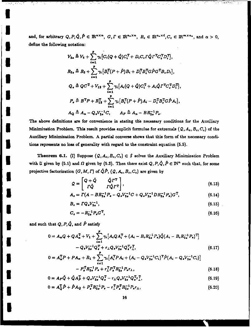
and, for arbitrary Q,PI,P E I,"', G,I E 1Rn.xn, B E lRn.xl,C E IE " ne, and a > O,

3 define the following notation:

P

v 2,. , 2 +E _r, [c(Q + O)c + Dc.rNrTc.TDJ,

Pm 4~=1 IIR 2.'L R2 +E -i [B(p + P)B, + D?~BTGfGTB.Di],

Q. -QCT+ + T, Q+¢c + AQrTc.D:9I q.4cT~1 2 +Z A.(Q + 4)CTP

p4BTP + R12 + -[B?(P + P),- D.7B.GPA4],

Aq AA. - Q.V;'C, Ap A A. - BR.Po.

The above definitions are for convenience in stating the necessary conditions for the Auxiliary

3 Minimization Problem. This result provides explicit formulae for extremals (Q, A., B., Cc) of the

Auxiliary Minimization Problem. A partial converse shows that this form of the necessary condi-

3 tions represents no loss of generality with regard to the constraint equation (5.5).

Theorem 6.1. (1) Suppose (Q, A., B., C.) E S solves the Auxiliary Minimization Problem

with U given by (5.1) and £7 given by (5.3). Then there exist Q,P, 1, P E IN' such that, for some

projective factorization (G, M, r) of 4P, (Q, Ae, B0 , Cc) are given by

LQ Jae iveTn (6.13)N=Lr rOrT

3 A. = r(A - BRj*'P. - q.Vi;1.C + Q.Vj2 1DR-'P.)GT, (6.14)

B. = rQ.Vi-1, (6.15)

SC=" -R-PGT, (6.16)

3 and such that Q,P,q4, and P satisfy

P0 AaQ +QAi +Vi+ ,[iQ4Ai(,- B RF.)(A. -B, RFP.)T}

I-Q.V2qT+r±. T -1qyrC,Q°V2 Q°+ rQoV2 Q~i., (6.17)

0 = AOP + PA, + RI + Z-4[ATPAi + (A,-iQV 2 ;C,)T?(A -Q°V 2;1c,)]

- P.TRj.P. + rTPT7- . .Pr, (6.18)

I o = Ap + QAp + PrQR.V: -0 (6.1)

3= AP+ PAq + PIRj.1 P. - r±P"RjLP.r±, (6.20)

16I

Irankq= rankP= rank (=n.. (6.21)

Furthermore, the auxiliary cost is given by 3J(.Q,A,B., C.) = tr[(Q + 4)RI - 2R 12R 1 P.Q + PTR-1 R2Rj 1 P,Q]. (6.22) 1

(II) Conversely, if there exist Q,P,&,P E INn satisfying (6.17)-(6.21) with B. and C, given 3by (6.15) and (6.16), then (Q, A., B.,C.) given by (6.13)-(6.16) satisfy (4.2) and (5.5) with

.(Q,A.,B.,CC) given by (6.22).

Proof. See Appendix B. 0

Remark 6.1. Theorem 6.1 presents necessary conditions for the Auxiliary Minimization Prob- Ilem which explicitly characterize extremal quadruples (Q, A., B, C,). These necessary conditions

consist of a system of two modified Riccati equations and two modified Lyapunov equations coupled 3by both the optimal projection r and uncertainty bounds. If the uncertainty bounds are deleted,

then the results of [HBI are recovered. I

Remark 6.2. When solving (6.17)-(6.21) numerically, the uncertainty termr can be adjusted

to examine tradeoffs between performance and robustness. Specifically, the bounds ai and the

structure matrices A, B, C, and Di appearing in V2., R 2 , Q., and P. can be varied systematically Uto determine the region of solvability of (6.17)-(6.21).

Remark 6.3. Although equations (6.17)-(6.21) appear formidable, they are, in fact, quite nu- 3merically tractable. For related problems involving coupled Riccati equations, homotopic corfinu-

ation methods have been shown to be effective ([KLJ],[MB]). Similar algorithms for solving (6.17)- 1(6.21) have been developed in [GHI,[R], while iterative algorithms are discussed in [G2J,[GVI,[CY].

Remark 6.4. Because of the presence of B, and C, in the definitions of V2., R 2 .,Q., and 3P., the optimality conditions (6.17)-(6.20) are coupled with the gain expressions (6.15) and (6.16)

for B, and C.. When the problem is specialized to the case Di = 0, i = 1,... ,p, this coupling |disappears and equations (6.17)-(6.20) can be solved without reference to the gain expressions

(6.15) and (6.16).

7. Sufficient Conditions for Robust Stability and Performance

In this section we combine Theorem 3.1 with Theorem 6.1 (II) to obtain our main result Uguaranteeing robust stability and performance.

17

I

II

Theorem 7.1. Suppose there exist Q,P,(/,P E IN4 satisfying (6.17)-(6.21) with B, and

I C. given by (6.15) and (6.16). Then, with (Q, AC, B.,C.) given by (6.13)-(6.16), (A +!%A, I +

J2(Q,B.,C.) - (4dAQ + QAT)1*) is stabilizable for all (AA,AB,!%C, AD) E U if and only if

A + AA is asymptotically stable for all (!%A, !B,AC, AD) E U. In this case, the performance

(2.7) of the closed-loop system (2.9) satisfies the bound

IJCJ(A.,Be,C) :_ tr[(Q+4)Rj-2R]L2 R'P + P7RRRR .P,]. (7.1)

I Proof. The converse portion of Theorem 6.1 implies that Q given by (6.13) is nonnegative defi-

nite and satisfies (5.5) or, equivalently, (3.4). It now follows from Theorem 3.1 that the stabilizabil-3 ity condition (3.5) is equivalent to the asymptotic stability of A+AdA for all (AA, AB, AC, AD) E U.

In this case Proposition 4.1 yields robust stability and performance. The robust performance bound3 (7.1) is a restatement of (4.3) utilizing (6.22). 03

Note that Theorem 7.1 is constructive in nature rather than existential. Specifically, Theorem

7.1 involves a coupled system of modified Riccati/Lyapunov equations (6.17)-(6.21) whose solutions,

when they exist, are used to explicitly construct the dynamic feedback gains (6.14)-(6.16) which

are guaranteed to provide both robust stability and performance. The following existence result

concerns the solvability of (6.17)-(6.21). Let n, denote the dimension of the unstable subspace of

I the plant dynamics matrix A.

5 Theorem 7.2. Assume n, _ n,, R, > 0, V > 0, suppose the nominal plant, i.e., (2.1), (2.2)

with ai = 0, i = 1,... ,p, is stabilizable and detectable and, in addition, is stabilizable by means

of an n~th-order strictly proper dynamic compensator (2.3),(2.4). Then there exist &z,..., &, > 0

such that if oj E [0, d), i = 1,... ,p, then (6.17)-(6.21) have a solution Q, P, , P E INn for which

(A., B., C.) given by (6.14)-(6.16) solves the Robust Stability Problem with robust performance

bound (6.22)

Proof. From Theorem 3.1 of [R1I,[R2] it follows that there exists a solution to (6.17)-(6.21)

which stabilizes the nominal plant. By continuity there exists a neighborhood over which robust

3 stability with performance bound (6.22) holds. 0

Theorem 7.2 is an existence result which guarantees solvability of the sufficiency conditions3 over a range of parameter uncertainties. The actual range of uncertainty which can be bounded

and the conservatism of the performance bound are, of course, problem dependent.

118

I

II

8. Specialization to Full-Order Dynamic Compensation

To draw connections with standard full-order LQG theory, we specialize the results of Sections 16 and 7 to the full-order case, i.e., n. = n. As discussed in [HB], in the full-order case G = F-1

and thus G = r = r =/, and r± = 0 without loss of generality. To develop further connections Uwith standard LQG theory assume I

R 1 2 =0, V1 2 =0, D=AD=0. (8.1)

Since AD = 0 we shall write (AA,AB, AC) in place of (AA,AB,AC,AD). Also, for arbitrary 3Q, P, 1, P E IRnXn and a > 0 define the following notation:

p p

qA -QCT+ ,A,(Q + )C, P. A BTP + ,BT(P + P)A,,i=1 i=I1

AQ A A. - Aa1.1 c, A A. - BA-P.. 3Theorem 8.1. Let n, = n, assume (8.1) is satisfied, and suppose there exist Q, P,( ,P E IN"

satisfying

0=-- A.Q + QAa + V, + y7, [A.QA?'+ (A, - BA- .P.)Q(Aj - BfAt1-. )'r] - (8.2)P

ATP + PA. + R, + yj [ATPA. + (A. - q .tlC,)TP(A. - Q ' jC)] - .TA-1 , P. (8.3) 30 A4 + + #1 (8.4)

0 =A TP + P A + P.Tj 1 P., (8.5)

and let (Q,AC,B.,C) be given by 3Q[ +10 2] (8.6)3

A. = A - BR: P. - .,: ' (8.7)B, = A; ",(8.8) 3

C = - I P .. (8 .9 )

Then, (A+ AA, [ + f(Q, B,C.) - (AkQ + Q0AT)]&) is stabilizable for all (AA, AB, AC) E U if

and only if A+AA is asymptotically stable for all (AA, AB, AC) E U. In this case the performance 319 I

I.U

of the closed-loop system (2.9) satisfies the bound

n J(AC, BC,CC) .5 tr[(Q + e )RI + Pbfa R L] (8.10)

n Proof. The proof follows from the reduced-order case given in Appendix B. 0

3 Remark 8.1. Theorem 8.1 presents sufficient conditions for robust stability and performance

for full-order dynamic compensation. These sufficient conditions comprise a system of two modified

Riccati equations and two Lyapunov equations coupled by the uncertainty bounds. This coupling

illustrates the breakdown of regulator/estimator separation and shows that the certainty equiva-

lence principle is no longer valid for the LQG result with real-valued structured plant parameter

variations. If, however, the uncertainty terms A.-, B1 , C are set to zero, it can be seen that (8.4)

and (8.5) drop out, while (8.2) and (8.3) reduce to the standard separated Riccati equations of

LQG theory.

3 9. Illustrative Numerical Example

To demonstrate the above results we present an illustrative numerical example. The example3 chosen was originally used in tD] to illustrate the lack of a guaranteed gain margin for LQG

controllers. This example was also considered in [BG1] for a preliminary robustness study. Define

n=2, M=t=p= 1,

3 A -- [1 ], B=[0] , C=[1 0], D=0,

0 1 1o3 R=V =" 60] , R 1 2 = V. 2 R2=V2

Note that the system is open-loop unstable and becomes unstabilizable at a, -1. As can easily

be seen using root locus, a strictly proper stabilizing controller must be of at least second order.

Hence we consider (6.17)-(6.21) with n. = n and thus ri- = 0. Using algorithms described in

3 [GH],[R], controllers were obtained for (a, a,) = (.1,.1), (.4,.2) and (1.6,.4). Figure 1 compares

the guaranteed robust stability region to the actual robust stability region. Note that the design

approach yields greater stability than is guaranteed a priori. This phenomenon is not surprising

since even the LQG result may provide arbitrarily high levels of robustness for particular problems

while failing to guarantee even minimal robustness for all problems. These results thus demonstrate

20

I

Ithe ability of the theory to robustify the LQG result. Interestingly, the form of the actual stability

region mimics the classical 6 dB downward/infinite dB upward gain margin of full-state-feedback

LQR controllers. Finally, Figure 2 compares guaranteed closed-loop performance to actual closed-

loop performance over the guaranteed closed-loop robust stability region. Controller gains are given 3in Table 1.

Acknowledgment. We wish to thank Jill M. Straehla for preparing the manuscript version 3of this paper and Scott W. Greeley for carrying out the numerical computations.

2IIIIIiIIiiUI

21

3

7.0

6.0

5.0

I 4.0

3.0 -ACTUAL CLOSED-LOOP ROBUST STABILITY*2.0 -REGION

GUARANTEEDCLOSED-LOOP£1.0 RBSREGION[-ti

3 0.0

-1.010.0 0.1 0.2 0.3 0.4 0.5

Figure 1

losGUA ANT ED PER ORM NC

0~

STBIIT RPiO FORANC Ja.,),

03. 0 . . . .

FigureI

IIi

( )A c Bc C¢

-14.917 1.0 15.917(.1..) - 71 1-15.2182 -4.9657]

-8.17 3.9657 79.959I

17.963 1.0 18.963(.4..2) -[ j [1 (-6.6011 -5.4614]

I I .6.., [-4.-087.3 -6.543 1073.5 U-_.____ -,._,_

I5 Table 1

III1II1

APPENDIX A: Proof of Lemma 6.1

(i) Clearly eP and P MP have the same nonzero i envalues. Since P*(5A is nonnegativei

definite, IOP ha. nonnegative eigenvalues.

(ii) The result follows from Theorem 6.2.5 of (RMI, p. 123. See also Theorem 4.3 of [G 1].

(iii) This result follows from (ii) and (8.1). 3(iv) This result follows from the definition of the group generalized inverse (see [CM]). Alternatively,

let OP = IDF , where # e D(OP), D = diag(dl,...,d.). Then (4P)1 = #DOt , where ID# =/dif A0, andD =Oif =O, i= 1,...,n. Hence #P l i=sE -D(ii) =(Id00

idempotent, where E is a diagonal matrix with r ones and n - r zeroe on the diagonal. Clearly,

(6.3) is valid.

(v) Without loe of generality choose t in the preceding argument so that D = blocd-diag(b,o._,),

when b=diag(J,,...,e), >, i= ,...,,. Hence

p =f b Oon) x r -I, O

and thus (6.5) holds with

G=[I, o,x(._,)]VT, M=b, r=[r, orx(%_)jiP- 3(vi) Sylvester's inequality and (6.4) imply that I

r = rank QP6 !5 {rank G, rank M, rank r} _< r,

which yields (6.6). The expression (6.7) for (4p^)* follows directly form the definition of the

group generalized inverse. Furthermore, (6.2), (6.5) and (6.7) imply (6.8), while (6.5) and (6.8)

imply (6.9). 3(vii) Let both (G, M, r) and an identically dimensioned triple (C6, 9f, t) satisfy (6.4). Then it is

easy to verify that - S-1 G, lAf = SMS- 1 and t = Sr, where S = PGT and S - 1 = V(?T I(viii) It follows from (ii) that there exists TI E C((5, P) such that 3

IF D4 Otx(n-.r)] tT, P -T [o(pX Orx(n..r)] I- 1 ,O0(n-rlxr Oft-P IT = O(n-rlxr On-P I i

22

I

I.

i I ..f [.. ,)* [ ,x,-, )iI

- - (.D!) t(..)

LO( n-r)xr 0-

u ~and thus ~ (P.Finally, (8.10) and (8.11) are imanediate. C3

I.I

I

IIII

I II i

I

APPENDIX B: Proof of Theorem 6.1

To optimize (4.10) over the open set $ subject to the contraint (5.5), form the Lagrangian

C(,EB,.PA t{Q+[~Q+Q P+~1 AQ~ I} (B.1)

where the Lagrange multipliers A > 0 and P E R110 are not both zero. We thus obtainaz lW-Q 12 Ap +pA.+ A~';. Ak(B-2)

Setting az/OQ = 0 yields

=Al+ A. E fiAPA +r?(B.3)3

or, equivalently,

Since A is assumed to be stable, AT is invertible, and thus A = 0 implies P = 0. Hence, it can be

assumed without los of generality that A = 1. Furthermore, it follows from Proposition 5.2 with

A,V replaced by AT, I that P is nonnegative definite.

Now partition fi x fi Q, P into n x n, n x n., and n. x n. subblocks as

[2= P 2 3and define the positive-definite matrices 3

p p

V V2 + ,,CiQ1C + DC.Q:C.D , R2 . - R2 + "i[BPBi + D B PzBD].-1=1 l

Thus, the stationarity conditions for A., B., C. are given by

az _ pLQBe + p2Q2 = 0, (B.4) 3

B. = A B.BV2. + (P,2 Q, + P 1q,)cT

+P [V12 + y(A.Q 1CT + A.Q 12CTD] =0, (B.5)

ac. + I

+ 2 [R-+ iy(BTP1Ai + D'TPITA)]Q1 2 =0. (B.6)24 I

' -- I ii , I I II I I U

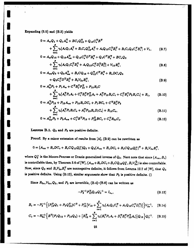
IExpanding (5.5) and (B.3) yields

I o=.Q +QIA+ BC.Q, + Q1 2CB

+ F ',[A.QzA T + B,C.QTA' + AQ13CIB, + B,C.Q 2 CTB.7 + Vt, (B.7)S=A.Q,, + Q,,AT + Q1,CI!DTBT + QICTB. + BC.Q,

+ , I,[A-Q1ciCB. + A-Q,C7DTB,1 + V 12BT, (B.8)i=1

I0o = A, A e A + B.Cq 12 +qCTBT+ B.DC.Q,

+ Q,CTDTET + BV 2 B , (B.9)

I 0= AlP + PA, + CTB.TPT + P 2B.C

+ yitATPA. + CTBTP&A. + AT)P12 B.C. + CBTP2 B.Cj] + R,, (B.10)

0 = A.P1+P 1 2 A.. + P12 B.DC. + P1BC. + CTBTP

+ [PBAc. + ATP 2 B.D,C. + R12C., (B.11)

o A 2 + p 2A. + C.BTP1, 2 + PITBC. + CTR,-C0 . (B.12)

Lemma B.1. Q2 and P2 are positive definite.

I Proof. By a minor extension of results from [A], (B.9) can be rewritten as

I o =(As. + B.DCG + B.CQ12Q2+)Q 2 + Q2(A.. + B.DC. + B.CQ12Q+)T + BV 2.BT,

where Qt is the Moore-Penrose or Drazin generalized inverse of Q2. Next note that since (Ac, B")

is controllable then, by Theorem 3.6 of [W], (A..+ B.DC.+B.CQI:Q + , BCVt) is also controllable.Now, since Q2 and B.V2.B are nonnegative definite, it follows from Lemma 12.2 of (W], that Q23is positive definite. Using (B.12), similar arguments show that P2 is positive definite.

3Since R 2.,V 2.,Q 2 , and P2 are invertible, (B.4)-(B.6) can be written as

-PsjPTq1 2 Q[l = I.., (B.13)

12{(P Q, +2P, q)cT+P [V,2 + Z ji(A.QC? + AQnCTD)]}V.LI , (B.14)

-1~~~~~~~ 11Tpq2+p22 R

C. =-R2; {BT(Plel + P1 2q,) + [12 + y,(B7,PA,, + DTB Pj2A)]Q,,}Q-'. (B.15)

25I

I

Now define the n x n matrices

- 1 2 P - P12 P; I,

A- Q -I QT,, 2 P 2 P ;, I PIT

r" -! - 1 2V~ -tIT

and the n, x n, n. x n., and n, x n matrices I

GAQ- 1q ,, MQ 2 P, r=-P 1 PT.

Note that r = GTr.

Clearly, Q, P, 4, and P are symmetric and 4 and P are nonnegative definite. To show that Q

and P are also nonnegative definite, note that Q is the upper left- hand block of the nonnegative- 3definite matrix Q Q Q T, where -= 1 -Q"Q!']I

O. . ].

Similarly, P is nonnegative definite.

Next note that with the above definitions, (B.13) is equivalent to (6.5) and that (8.4) holds.

Hence r = GTF is idempotent, i.e., r2 = r. Furthermore, it is helpful to note the identities

=Q 12G =GTQT~ = GTQ 2 G, P = -P 1 2 r = -r.TPT, = r Tp2 r (B.16)12 G T..GT, rr= r, (B.17)

ST=Q -, P = Pr, (B.18) 30P= -Ql2PI. (.19

Using (B.13) and Sylvester's inequality, it follows that

rank G = rank r = rank Q12 = rank P12 = n.

Now using (B.16) and Sylvester's inequality yields

n. = rank Q12 + rank G - n. rank ( : rank Q12 = n.,3

which implies that rank ( = n.. Similarly, rank P = n,, and rank (/P = n, follows from (B. 19). 326

I

I.

The components of Q and P can be written in terms of Q, P,1,,G, and r as

I Q 1 =Q-+ , P 1 =P+P, (B.20)Q ,2 T P12 = -PGT, (B.21)

Q2 = rrT, P2 = GPGT. (B.22)

3 The expressions (6.13), (6.15), and (6.16) follow from the definition of Q, (B.14) and (B.15).

Substituting (B.20)-(B.22) into (B.7)-(B.12) yields[pI0 = A.Q + QA+l+ V + >3 [AQA T + (A - BiR-*1P.) (A - BiR;.P.)T]i=1

3Ap + 4A+, (B.23)

o = [Ap4 + 4(GTAC=r + q.v.rC)T + q.v2;q.] rT (B.24)

0 o = rP[(GTA..J + q.Vi-.C)4 + 4(GTAC.r + Qr V;C)T+ q.v',q.T r (B.25)

0= ATP + PA, + RI + -1i [ATPA. + (A. - Q.V lC,)Tf(A - Q.V2.'C)]

T + AA ,AQ (B.26)

3 0= [ATP + P(GTAo.F + BR. 1P.) + P7Ri.lP.]GT, (B.27)

O= G[(GTA,,r + BR;,*P.)TP + P(GTAOF + BR;*P.) + PTp.P,]GT. (B.28)

I Next, computing either r(B.24) - (B.25) or G(B.27) - (B.28) yields (6.14). Substituting this

expression for Ac into (B.23), (B.24), (B.27) and (B.28) it follows that (B.25) = F(B.24) and3 (B.28) = G(B.27). Thus, (B.25) and (B.28) are superfluous and can be omitted. Next, using

(B.23) + GTr(B.24)G - (B.24)G - [(B.24)G]T and GTF(B.24)G - (B.24)G - [(B.24)G]T yields

(6.17) and (6.19). Using (B.26)+rTG(B.27)r-(B.27)I-[(B.27)rT and ITG(B.27)r-(B.27)r -

[(B.27) r]T yields (6.18) and (6.20).

I Finally, to prove the converse we use (6,13)-(6.21) to obtain (5.5) and (B.3)-(B.6). Let

A.,B,C.,G,r,rQ,P,^,P, Q be as in the statement of Theorem 6.1 and define QI ,QI 2,Q 2,P1 ,

IP 12,P2 by (B.20)-(B.22). Using (6.5), (6.15) and (6.16), it is easy to verify (B.5), (B.6). Finally,

substitute the definitions of Q, P, Q, P, G, and r into (6.17)-(6.20), reverse the steps taken earlier

Iin the proof, and use (6.13)-(6.16) along with (6.5) and (6.8)- (6.11) to obtain (5.5) and (B.3).

Fin ally, note that n [ 0]°

which shows that Q >0 thus verifying (4.2). 0

271

References

[A] A. Albert, "Conditions for Positive and Nonnegative Definiteness in Terms of Pseudo Inverse," 3SIAM J. Appi. Math., Vol. 17, pp. 434-440, 1969.

[AM] B.D.O. Anderson and J.B. Moore, Linear Optimal Control, Prentice-Hall, Englewood Cuffs,NJ, 1970.

[BI] B.R. Barmish, "Necessary and Sufficient Conditions for Quadratic Stabilizability of an Uncer-tain Linear System," J. Optim. Thy. Appi., Vol. 46, pp. 399-408, 1985.

[B2] D.S. Bernstein, "Robust Static and Dynamic Output-Feedback Stabilization: Deterministic andStochastic Perspectives," IEEE Trans. Autom. Contr., Vol. AC-32, pp. 1076-1084, 1987. 3

[B3] J.W. Brewer, "Kronecker Products and Matrix Calculus in System Theory," IEEE Trans. Circ.Sys., Vol. CAS-25, pp. 772-781, 1978.

[BCL] B.R. Barmish, M. Corless, and G. Leitmann, "A New Class of Stabilizing Controllers forUncertain Dynamical Systems," SIAM J. Contr. Optim., Vol. 21, pp. 246-255, 1983.

[BG1] D.S. Bernstein and S.W. Greeley, "Robust Controller Synthesis Using the Maximum Entropy IDesign Equations," IEEE Trans. Autom. Contr., Vol. AC-31, pp. 362-364, 1986.

[BG2] D.S. Bernstein and S.W. Greeley, "Robust Output-Feedback Stabilization: Deterministic and 3Stochastic Perspectives," Proc. Amer. Contr. Conf., pp. 1818-1826, Seattle, WA, June 1986.

[BH1 D.S. Bernstein and D.C. Hyland, "The Optimal Projection Equations for Finite-DimensionalFixed-Order Dynamic Compensation of Infinite-Dimensional Systems," SIAM J. Contr. Op-tim., Vol. 24, pp. 122-151, 1986.

[BH2] D.S. Bernstein and W.M. Haddad, "The Optimal Projection Equations with Petersen-HollotBounds: Robust Stability and Performance via Fixed-Order Dynamic Compensation for Sys-tems with Structured Real-Valued Parameter Uncertainty," IEEE Trans. Autom. Contr., Vol.AC-33, pp. 578-582, 1988.

[BH3] D.S. Bernstein and W.M. Haddad, "Robust Stability and Performance Analysis for State SpaceSystems via Quadratic Lyapunov Bounds," submitted. 3

(BHK] S.P. Bhattacharyya, J.W. Howze, and L.H. Keel, "Stabilization of Linear Systems with Fixed-Order Controllers," Lin. Aig. Appi., Vol. 98, pp. 57-77, 1988.

[CL] M. Corless and G. Leitmann, "Continuous State Feedback Guaranteeing Uniform Ultimate

Boundedness for Uncertain Dynamical Systems," IEEE Trans. Autom. Contr., Vol. AC-26,pp. 1139-1144, 1981. 3

[CM] S.L. Campbell and C.D. Meyer, Jr., Generalized Inverses of Linear Transformations, Pitman,London, 1979.

[CP] S.S.L. Chang and T.K.C. Peng, "Adaptive Guaranteed Cost Control of Systems with UncertainParameters," IEEE Trans. Autom. Contr., Vol. AC-17, pp. 474-483, 1972.

(CY] M. Cheung and S. Yurkovich, "On the Robustness of MEOP Design Versus Asymptotic LQG ISynthesis," IEEE Trans. Autom. Contr., Vol. 33, 1988, to appear (also, Proc. Amer. Contr.Conf., pp. 24-29, Atlanta, GA, June 1988). 3

I

(D] J.C. Doyle, "Guaranteed Margins for LQG Regulators," IEEE .Trans. Autom. Contr., Vol.JR AC-23, pp. 756-757, 1978.

[ER] M. Eslami and D.L. Russell, "On Stability with Large Parameter Variations: Stemming fromthe Direct Method of Lyapunov,x IEEE Trans. Autom. Contr., Vol. AC-25, pp. 1231-1234,1980.

(G11 K. Glover, 'All Optimal Hankel-Norm Approximations of Linear Multivariable Systems andTheir Lw-Error Bounds,* Int. J. Contr., Vol. 39, pp. 1115-1193, 1984.IG2] A. Gruzen, 'Robust Reduced Order Control of Flexible Structures," C. S. Draper LaboratoryReport #CSDL-T-900, April 1986.

1 [GB] A.R. Galimridi and B.R. Barmish, 'The Constrained Lyapunov Problem and Its Applicationto Robust Output Feedback Stabilization," IEEE Trans. Autom. Contr., Vol. AC-31, pp.410-419, 1986.

JGH] S.W. Greeley and D.C. Hyland, 'Reduced-Order Compensation: LQG Reduction Versus Op-timal Projection Using a Homotopic Continuation Method," Proc. IEEE Conf. Dec. Contr.,pp. 742-747, Los Angeles, CA, December 1987.

(GV] A. Gruzen and W.E. Vander Velde, "Robust Reduced-Order Control of Flexible StructuresUsing the Optimal Projection/Maximum Entropy Design Methodology," AIAA Guid. Nay.Contr. Conf., Williamsburg, VA, August 1978.

[H] W.M. Haddad, Robust Optimal Projection Control-System Synthesis, Ph.D. Dissertation, De-partment of Mechanical Engineering, Florida Institute of Technology, Melbourne, FL, March1987.

[HB] D.C. Hyland and D.S. Bernstein, "The Optimal Projection Equations for Fixed-Order DynamicCompensation," IEEE Trans. Autom. Contr., Vol. AC-29, pp. 1034-1037, 1984.

[KBJ 0.1. Kosmidou and P. Bertrand, 'Robust-Controller Design for Systems with Large Parameter3 Variations," Int. J. Contr., Vol. 45, pp. 927-938, 1987.

(KBHI L.H. Keel, S.P. Bhattacharyya, and J.W. Howze, "Robust Control with Structured Perturba-tions,* IEEE Trans. Autom. Contr., Vol. 33, pp. 68-78, 1988.

[KLJ] P.T. Kabamba, R.W. Longman, and S. Jian-Guo, "A Homotopy Approach to the FeedbackStabilization of Linear Systems," J. Guid. Contr. Dyn., Vol. 10, pp. 422-432, 1987.

[LI G. Leitmann, "Guaranteed Asymptotic Stability for a Class of Uncertain Linear DynamicalSystems," '. Optim. Thy. Appl., Vol. 27, pp. 99-106, 1979.

[MB] M. Mariton and R. Bertrand, "A Homotopy Algorithm for Solving Coupled Riccati Equations,"Optim. Contr. Appl. Math., Vol. ,3, pp. 351-357, 1985.

[PH] I.R. Petersen and C.V. Hollot, "A Riccati Equation Approach to the Stabilization of UncertainSystems," Automatica, Vol. 22, pp. 397-411, 1986.

(RI] S. Richter, 'A Homotopy Algorithm for Solving the Optimal Projection Equations for Fixed-Order Dynamic Compensation: Existence, Convergence and Global Optimality," Proc. Amer.Contr. Conf., pp. 1527-1531, Minneapolis, MN, June 1987.U

I

[R21 S. Richter, "Reduced-Order Control Design via the Optimal Projection Approach: A HomotopyAlgorithm for Global Optimality," Proc. Sixth VPI8SU Symp. Dyn. Contr. Large Str., L.Meirovitch, Ed., pp. 17-30, Blacksburg, VA, June 1987. 3

[RM] C.R. Rao and S.K. Mitra, Generalized Inverse of Matrices and Its Applications, John Wileyand Sons, New York, 1971. 3

[TB] J.S. Thorp and B.R. Barmish, "On Guaranteed Stability of Uncertain Linear Systems viaLinear Control," J. Optim. Thy. Appl., Vol. 35, pp. 559-579, 1981.

[VWI A. Vinkler and L.J. Wood, 'Multistep Guaranteed Cost Control of Linear Systems with Un- Icertain Parameters," J. Guid. Contr., Vol. 2, pp. 449-456, 1979.

EWI W.M. Wonham, Linear Multivariable Control: A Geometric Approach, Springer-Verlag, NewYork, 1979.

IIIIIi

UI,IIIII

II

INT. J. CONTROL, 1988, VOL. 47, NO. 4, 1117-1132

I IUnified optimal projection equations for simultaneous reduced-order,robust modelling, estimation and control

WASSIM M. HADDADt and DENNIS S. BERNSTEINt

An optimal design problem which unifies reduced-order modelling, estimation andcontrol problems is stated. Necessary conditions for optimality are obtained in theform of a coupled system of modified Riccati and Lyapunov equations. The resultspermit treatment of several new problems, such as reduced-order dynamic compen-sation with partially known disturbances and unified reduced-order control andestimation. Upon appropriate specialization, results obtained previously for theindividual problems of reduced-order modelling, estimation and control arerecovered. An additional feature is the inclusion of parameter uncertainty bounds sothat the necessary conditions for an auxiliary minimization problem serve assufficient conditions for simultaneous robust, reduced-order modelling, estimationand co.-.rol.

Notation and definitionsNote. All matrices have real entries.

R; R"' 1 ; R' real numbers; r x s real matrices; R"'S( ) r x r identity matrix, transpose

; Kronecker sum; Kronecker product (Brewer 1978)r x r symmetric matrices

I1' r x r symmetric non-negative-definite matricesPIP r x r symmetric positive-d-inite matrices

ZI 1< Z2 Z2 -Z1E 4', Z1,Z 2 E A'Z,<Z2 Z 2 -Z6P, Z 1,Z 2 e"

asymptoticallystable matrix matrix with eigenvalues in open left half-plane

n, m, dt, 1, F, nc, q, p positive integersi n+nc

X, u, y, ) , x,, y., y., i n, m, 1, f, n, q, f, rf-dimensional vectorsA, AA; B, AB; C, AC n x n matrices; n x m matrices; I x n matrices

AI, Bi,C nxn, nxm, Ixnmatrices, il. p6,, a, positive numbers, i = 1, ..., p

A. A + 2 ii, I,Ac ,, B., Cc, C.,C., nn, ncx 1,nxt, m x n, q xn,, rxnc ariefl ~~ ,CeC

, (f n x , ,I x n matrices

L q x n matrix

Received 9 March 1987. Revised 20 May 1987.t" Department of Mechanical Engineering, Florida Institute of Technology, Melbourne, FL

32901, U.S.A.T Harris Corporation, Government Aerospace Systems Division, Melbourne, FL 32902,I U.S.A.

I

1118 W H adnd O BeS&nitn

R estimation-eror weighting Pinmodel-error whtiitmg i tP'

R, state weighting matri inoR control we4hting matx in P 1R IZ u x nm ciuroweightng m4arm n h thatR1 - Rl R 1'X,

4)0w( -) i .trensiocia white wxw inqiada of %,t- mrW

WA( • )I

w'(• n"dImensona white notw11") I-dimensional white nOiti

V, intensity of --,( -) in 1V, intensity ofS( ut• ) in PV, I A X I crow Intentl) of w, I. wIt IV intensty o ( inPE expected value

B[ C A. J ' 0 JP, L' A 'L+" + e'" Ae )t,;C -VA.IA

A TtIC'LCA C'R,C, RC.C*jr will) + 041)LB'wIII + B'O0l

Pr V, + AVAl, v,;+JsLB VII + B.v , , B +3

I. Imemdduc, ••

The problems of quadratkally optimal reduced-ordct modelling. estination andcontrol have been treated in a common framework by Hyland and Bernstein I 5).BeMstein and Hyland (1985). and Hyland and emsiein (1984). respecqivelySpecifically, by carrying out a judicious transformation o4 vanables. it was %bown thatthe necessary conditions for optimalty could be cast as coupled systems of 3 3 and 4 Imodified Lyapunov and Riccatt equations. respectively The coupling is Via an oblique

projection (i.e. idempotent matrix) which arises as a direct conlequence o(opomatyand which determines the geometric structure of the reduced-order modeL estimator. Ior compensator. When the order of the estimator or compensator is set equal to theorder of t plant. the additional modified Lyapunov equations drop out and theremaining modified Riccati equations reduce to the standard steady-state Riccati

equations of Kalman filter and LQG theory.An immediate benefit of this formulation of the necessary conditions is clanfi-

cation of the relationship between the operations of model reduction and estimator orcontroller design. Specifically. although the additional pair of modified Lyapunov Iequations arising in the reduced-order estimation and control problems are analo-gous to the pair of modified Lyapunov equations characterizing the optimal reduced-order model, these equations are now inextricably coupled with the modified Riccat1equations characterizing the estimator and controller design. Hence. because of the 1coupling, this approach is distinct from LQG controller-reduction techniques (see. for I

I

example, Liui and Anderson 1916, &M Jockhomr and Sahesmas 19131 A xvis.panson between the LQC recduction mthods rettemmi by Liu and Az&oe I19Wt~and the optimal projpstoc approach has been given by Greeley and Hytand t19581

The goal of the penpae istoudth mts baeli oiytt

upnappropriate specsalizauon. yields the r duced-oder inoddhn& ewtxauocontrol rmutts as specia casn. Thus is accomplinhed by defi"a eri Fraundperformance funictiogial which incorporates features of all thre cntwu Thuu theoptimiatio problem involves de numwS a stuwk redizsl-otde byutm whichI simultaneously serves as a reduced-order model. estimator and controller (or an) twoof thes as desired) The acesiary condutmms now take the formn of a coupled systerof two modified Lyapuwvi equations and two msodifid Riccai equatiotis wtich canbe specualied to the necessary coaditions obtained perviously lot the reduood-orvkrmodeling. estimation and control probleres

There are several miotivations for developing a unifie formulation encompastangall three reults. For example, tn the full-order cawe the certainty eqwivalenor principleimplies that the tatu of the optimal dynamic compentor are also optimal etimatesof the plant sutate Thu is defiely niot the can for an optimal reduced-ordercontroller in which the sts may boaw no resiemblance to The plant stt The unifiedformulation of the Preset paper. however. exptes the desire that oompeuatorstain also provide estmates of seete anet stan fcu recept to the full-

ordr cwsuc acompensatorwilgnrlybsuotmlfe aticycu"pon fview snethe design also serves as an estimator A similar lormulation has

benconsidered by Wilson and Kumar (198).Additional problem which can be handled to the unife setting involve reduovd

order estimation and control to the presenncre of partially k nown plant disturbancesI ~When measurements of disturbance components ame available durngS reAlsmeoperatiotn. such measurements can be used as inputs to the estimator or coetrolle toimprove performance. Note that this problem incorporates aspects of the model-reduction formulation in which the same while nosesgnal is injected into both theplant and the design system.

A practical motivation for the unified problem setting is convenience in developingnumerical algorithms for treating diflent probler.s In particular. a singlie algorithmI for solving the unifled optimal projection equaticis can readily be used (or all specialcases without reprogramming. (For discussions of numerical algonthms for theoptimal projection equations, wee Greeley and Hyland IMU. and Richter 1"7.)

An additional feature of the reutts given herein is the treatment of parmetricuncertainty in the plant mamrices, By bounding the effets of parameter uncertainty onworst-case system performance. the necesary coniditions rof optimality efiectivelyserve as sufficient conditions tot robust stability and performance. A similar approachI has been carried out by Bernstein and Haddad ( 1988). using structured stabilityradius bounds. In the present paper we use an alternative bound which corresponds toa right shift of the dynamics matrix (or equivalently, an exponential cost weighting) inI conjunction with multiplicative white-noise type terms. The effect of multiplicativenoise on the optimal projection equations has been developed by Bernstein andHyland (1988). In the present paper such underlying interpretations will be suppres-sed since only the bound per se will be needed. Hence, although we use the phrasemultiplicative white noise' for convenience in referring to the type of bound used. itshould be stressed that our treatment of parameter uncertainty is wholly deterinn-3 istic. (See Bernstein 1987 a, and Haddad 1987. for further background and discussion.)

1120 WM. Haddad and D. S. Bernem

2. Simdsama insv.e wdsrd , rbU-aot md'-Nn eadmtw sad remn Io tis section we state the 'robust performance problem' for multunous

reduced-order modelling. estimation and control along with related notation for lateruse. let U c R'*X R'X R"a denote the set of uDtan perturbaIoMs I(4A, AB. AC) of the noimnal system matrices A. B and C.

Robust performmnce probiemFor fixed m 4 u. determine (A,. B. B.. C,. C.. C.) such that. for the augmented

system consisting of the nth-order controlled and disturbed plant

,i(t)-(A+4AA)x()+(B+ &B)a4t)+ A 4)+w 1(t) rg(0. c ) (2.1)

with noisy and non-noisy measurements

Y(t) M(C + AQt) + WI(u (2.2)3

At) - l) (2-3)

and nth-order design system 3I,(t) - A.x,(t) + Bj$t) + B..4t) (2.4)

Ar) - C,x,(r) (2-5)

yO - C.x,(t) (2.6)

y.( - C.x,() (2-7)

the performance criterion 1J(A,. B,. B.,. C,. C,. C.) A J, + J,+, (2.8)

is minimized, where IJ, A sup lim sup E[x T(t)R xt) + 2X1()R,,u(t) + uT()Rl(t)] (2.9)

I&A.&.AC IU I-=

J, A sup lim sup E[L) - y,(t)] TR[L") - y()] (2-10)1AAA.&&O.U I

J. sup lir sup E(r) - y(o)]Tg j(t) - y.(r)] (2.11)

Remark 2.1Suppose there are no uncertainties present, i.e. AA, AB. AC - 0. By setting L- 0

and iC - 0, it follows that J, and J. play no role in the optimization problem when C,and C, are both taken to be zero. As will be seen in Theorem 6.1. this is indeed theoptimal solution in this case. If, furthermore, A -0. then the reduced-order dynamic-compensation problem of Hyland and Bernstein (1984), is recovered. If. alternatively.R, =0, R12 -,0. B-0. A-O and iC-0 then the reduced-order state-estimation 3problem of Bernstein and Hyland (1985) is obtained. Finally, setting R, = 0, R 1, = 01L = 0. V, - 0, B 0 and C - 0 yields the model-reduction problem considered byHyland and Bernstein (1985). !

Remark 22

Suppose L=O and iC -0 (so that with C, and C, both zero J, and J. are 1ineffective) but that 9 ' 0. In this case, a portion of the plant disturbance, which is

II

II

Unified optimal projection equations 1121

assumed to be measurable during on-line operation, is being fed directly into thecompensator. Hence this problem, which generalizes that of Hyland and Bernstein(1984), can be thought of as reduced-order dynamic compensation with partiallyknown disturbances. Similarly the case R - 0, R, 2-0, B - 0 and C - 0 but A , 0provides a generalization of Bernstein and Hyland (1985), which can be thought of asreduced-order state estimation with partially known disturbances.

For each variation (AA, AB, AC) e U, the augmented system (2.1)-(2.5) can be

written as

A o .- (A + AA)g(:) + 0(t), £ e [0, (X) (2.12)

where

j(1) [xT(t). ,(t)]T (2-13)

and %(t) is white noise with intensity Pe 14'.For the 'robust performance problem' the cost can be expressed in terms of the

second-moment matrix of R(t). The following result is immediate.iProposition 21

For given (A,, B., B., C,, C., C.) and (AA, AB, AC) e U the second-momentI matrix

i satisfies ) [(t) T(t)], t e [0, co) (2.14)

(t) - ( + AA ) + Q t()4 + "j)T + e [0, ) (215)Furthermore,

J(AB., B,.,C., C, C.)- sup lim sup tr ("(t)§ (216)i I 60A04 U I-O

3. Suciewt eoadion for robust staMft ad perfowmasceIn practice, steady-state performance is only of interest when the augmented

system is stable over U. The following result is immediate.

Lemma 3.1Suppose the system (2.12) is stable for all (AA, AB, AC) e U. Then

J(A,, B,, B., C,, C,, C.) = sup tr 0JA (3.1)(&4. 6A C) 6U3 where O e 141 is the unique solution to

0 = (A + A)O + OA(A +A) T + P (3.2)

Remark 3.1When U is compact, 'sup' in (3.1) can be replaced by 'max'.

3 Since it is difficult to determine J(A, B,, B,,, C,, C,, C.) explicitly, we shall seekupper bounds.

II

I1122 W. M. Haddad and D. S. Bernstein

Theorem 3.1Let (I: IA x R*- x R"-., be such that 3

AiQ + AATC QB" ,C,)

(AA,AB,AC) EU, (,B,C) eIQ'x R"x R ='k' (3.3)

and, for given (A, B, B., C,. C,, C.), suppose there exists 0 e 1i' satisfying

0 -O.A + 0iAT + f(, B", C) + P (3.4)Furthermore, suppose the pair (P1i2, . + A) is detectable for all (AA, AB, AC) e U.Then A + AA is asymptotically stable for all (AA. AB. AC) e U,

(X ,(AAAB, AC) e U (3.5)andI

J(A,, B, B., C,, C., C.) < tr Qf (3.6)

Proof IFor all (AA, AB, AC) e U, (3.4) is equivalent to

=( + AA)Q + (, + A )T + (, B,, C, AZ) + I (3.7)

where

'p(O, B C,A) A C,( ,B C) _ (AAI + o A T) I

Note that by (3.3), 'I(O, B,, C, AA) > 0 for all (AA, AB, AC) e U. Since ( Z ,/+ AA) is detectable for all (AA, AB, AC) e U, it follows from Theorem 3.6 of Wonham(1979), that ((P+ P(0,B ,C.,A.I))1I2,A+AI) is detectable for all(AA, AB, AC) e U. Hence Lemma 12.2 of Wonham (1979), implies that A + AA? is Iasymptotically stable for all (AA, AB, AC) E U.

Next, subtracting (3.2) from (3.7) yieldso = (A +,&A) (o. _ d,) + (Qa" (,Z/ + ,,ZTr + ,e(o B ., A/T&)

or, equivalently (since A + AA? is asymptotically stable),

Q- 1A=,= exp(A +AA)t '(Q, B, C, AZ) exp (+ Altdt 0

which implies (3.5). Finally, (3.5) and (3.1) yield (3.6). 0 I

Remark 3.2For the dynamic-compensation problem the result that A + AA? is asymptotically

stable for all (AA, AB, AC) e U is equivalent to robust stability of the closed-loopsystem. For the state-estimation and model-reduction problems, however, A + AA? islower block triangular (since B:-0) and block diagonal (since C = 0), respectively.Thus robust stability is equivalent to A, stable and A + AA stable for all(AA, AB, AC e U.

We also note a sufficient condition for the solution Q of (3.4) to be positive Idefinite. U

I

3 Unified optimal projection equations 1123

Proposition 3.1Let 0 be as in Theorem 3.1. let (A, Bc, B. Cc. C,, Ca.) be given, and suppose there

exists G eql' satisfying (3.4). If (V"2 ,A1+AA) is observable for some(AA, AB, AC) e U, then 0 is positive definite.

Proof

If (P1/2,4 + A.4) is observable for some (AA, AB, AC) e U. then, by Theorem 3.6

of Wonham (1979), ((IV + 'I(Q, B, , C,, AA)) t12 , A + AA) is also observable for thesame (AA, AB, AC) e U. It thus follows from (3.7) and Lemma 12.2 of Wonham(1979), that Q is positive definite. 0

Remark 3.3f P is positive definite then the detectability and observability hypotheses of

Theorem 3.1 and Proposition 3.1 are automatically satisfied.

I Remark 3.4Theorem 3.1 can be strengthened by noting that the detectability assumption is, in

a sense, superfluous. To see this, first note that robust stability concerns only theundisturbed system while P involves the disturbance noise. Hence robust stability isguaranteed by the existence of a solution C e iQ' satisfying (3.4) with P replaced by al,for some a > 0. For this replacement detectability is automatic (see previous remark).For robust performance, however, Q in (3.5) must be obtained from (3.4).

4. Uncertainty structure ad right shift muiplicative white noise bomdThe uncertainty set U is assumed to be of the form

U={(AA, BAC) e R x Rh = :AAx= R AA,,

ARB a, ~uB, AC= f iCt, ioI..8,,

U1 i,,

I where, for i= 1,...,p. A, e R",, B e R"XM and Cie R"" are fixed matrices denotingthe structure of the parametric uncertainty; 6, is a given uncertainty bound; and a, isan uncertain real parameter. The closed-loop system thus has structured uncertainty3 of the form

I where

A, B C,

To obtain an explicit gain expression for (A, , B,, B., C ,, C, C.) we require that

[B,#O.C,-=0], i=l,...,p (4.3)

That is, for each i e { 1, ..., p} either B, or C, is zero. Of course, both B, = 0 and C, = 0are possible for a given i, and there are no restrictions on A,.I

I

1I

1124 W. M. Haddad and D. S. Bernstein

Given the structure of U defined by (4.1) we can define the bound satisfying (3.3). 1Proposition 4.1

Let a,1 . ap be arbitrary positive scalars. Then the function

Co, B, Ql = 6,(a, + af,-1.41014,) (4.4)d-1

satisfies (3.3) with U given by (4.1).

ProofNote that

= ,(l6 1 )Q + ( - uG'O + Q,)

which, since Ij < 5 , implies (3.3). 01

5. Auxiliary minimization problemRather than minimize the actual cost (2.8), we shall consider the upper bound

(3.6). This leads to the following problem.

Auxiliary minimization problemDetermine (A., B,, 8, C,, C., C.) and CI lQ* which minimize

J(A,, B , B., C,, C., C., 0) A tr R (5.1)subject toI

o 0 = AQ + iAT + I ,,OAT) + P (5.2)

and1(p/2, A+ AA) is detectable, (AA, AB, AC) e U (5.3)

Proposition 5.1If (A,, B , B., C, C, C, ) is admissible, i.e. (A,, B,, B., C,, C,, C., 0) satisfies

(5.2) and (5.3), then A + AJ is asymptotically stable for all (AA, AB, AC) e U and

J(A,, B,, B., CC, C,, < J(A,, B,, B., C,, C,, C., Q) (5.4)

ProofWith D given by (4.4), Proposition 4.1 implies that (3.3) is satisfied. Furthermore,

admissibility implies that (3.4) has a solution 0e fA . Hence, with (5.3), thehypotheses of Theorem 3.1 are satisfied so that robust stability with the performancebound (3.6) is guaranteed. Note that with the definition (5.1), (5.4) is merely arestatement of (3.6). 0

6. Necessary conditions for the auxiliary minimization problemThe derivation of the necessary conditions for the 'auxiliary minimization

problem' is based upon the Fritz John form of the Lagrange multiplier theorem. II

I

Unified optimal projection equations 1125

Rigorous application of this technique requires additional technical assumptions.Specifically, we further restrict (A,, B,, B., C, C., C) to the set

S A {(A , B,, B, , C,, C., C., 0) : e P, A is asymptotically stable, and

(A,, B,, C) is minimal}where I A+ ./\ -. +

with, for convenience,

The following observation assures us that we can apply Lagrange multipliers over anopen constraint set.

Proposition 6.1I The set S is open.

ProofIt need only be noted that S is the intersection of three open sets. 5

Remark 6.1The constraint (A,, B,, B,, C,, C,, C., Q) e S is not required for either robust

stability or robust performance. As can be seen from the proof of Theorem 6.1 in theAppendix, the set S constitutes sufficient conditions under which the Lagrangemultiplier technique is applicable to the 'auxiliary minimization problem'. Specifi-cally, asymptotic stability of A serves as a normality condition which further impliesthat the dual P of Q is non-negative definite. Furthermore, (A,, B,, C) minimal is anondegeneracy condition which implies that the lower right n, x n, subblocks of Qand P are positive definite. It is extremely important to emphasize that Proposition5.1 implies that it is not necessary for guaranteed robust stability and performancethat an admissible quadruple, obtained by solving the necessary conditions, actuallybe shown to be an element of S.

For arbitrary Q, P, , e R define the following notation:

Rz. AR 2 + yBT(p + 1)Bi, V2, AV 2 It Y1CQ + )CJ

Q5 yQCT+V2+ ,A,(Q+ O)CT, P, -BTP+RI2 + tyBT(P+P)A,

Ae - A-QV-,C, ApA A,-BR-,XP,

The following factorization lemma is needed for the statement of the main result.

Lemma 6.1If 0, i e IQ" then Of' is diagonalizable with non-negative eigenvalues. If, in

addition, rank Of = n,, then there exist n, x n G, r and n, x n, invertible M such that

OP=G T Mr (6.1)

II

I1126" W. M. Haddad and D. S. Bernstein

rG T = 1,, (6.2) 3Furthermore, G, M and r are unique except for a change of basis in RF'.

Proof IThe result is an immediate consequence of Rao and Mitra (1971), Theorem 6.2.5,

p. 123. 3A triple (G, M, r) satisfying (6.1) and (6.2) will be called a projective factorization

of 0)5. Since Of' is diagonalizable it has a group generalized inverse (OP)' = GT M 'and

is an oblique projection. Furthermore, define the complementary projection 3Theorem 6.1 3

Suppose (A,, BCB,,, C, C,, C,,, Q) e S solves the 'auxiliary minimizationproblem'. Then there exist Q, P, Q, P5 e i" such that, for some projective factorization(G, M, F of 05, A,, B,, B., Cc, Ce, C. and Q are given by 3

A, = r(A - BR- 1 P, - Q.V- 1 C)G T (6.3)

B = rQV2;, (6.4)

B. = rb (6.5)

C, = - R2, P, GT (6.6)

Ce LG T (6.7)3C. = =GT (6.8)

r[Q+o r (6.9)

ro ror T

and such that Q, P, ( and Is satisfy 3o = A~Q + QA. + v1 + yI[AQAT + (A, - BR-' P)Q(A, - BiR 'p)T]

i~l I_Q. V2; Q T+ TI[Q. V7 QT + a~v6] T3 (.1

=AP + PA, + R, + [AiPA + (Al- QVC) T (A - Q. V2 'C , )i - I

-1 2 Tr T (6.11)0 -AP, R+ P + [P, Rz, P LR + ~LTR L + [~iS . TRO=A T+f + P T2 Pe L R + ' I T e -A

f'A+PR-'.+ RL J[PnR2 -P, + LT RL + TR,]r

(6.13)

rank 0 = rank P = rank OP = n, (6.14) 3

I

IUnified optimal projection equations 1127

For the proof see the Appendix.

I Remark 6.2As in Remark 2.1 suppose AA, AB, AC=0. By setting L= 0, B =0 and C = 0,

(6.10)-(6.13) specialize to the optimal projection equations (2.18)-(2.21) derived byHyland and Bernstein (1984), with the added features of correlated plant/measure-ment noise (V1 2 ) and cross weighting (R12). If R1 = 0, R12 = 0, B = 0, B = 0 and C = 0then, since P, = 0, (6.11) drops out and the remaining equations (6.10), (6.12) and(6.13) specialize to (2.10)-(2.12) of Bernstein and Hyland (1985). Finally, if R, = 0,R 1 2 = 0, L= 0, V = 0, B = 0 and C = 0, then, since Q, = P, = 0, (6.10) and (6.11) dropout and the remaining equations (6.12) and (6.13) specialize to (2.21) and (2.22) ofHyland and Bernstein (1985).

Remark 6.3more restrictive formulation for unified modelling, estimation and control is to

require C, = C, = C. so that u = y, = y,. In this case the three outputs of the designsystem (2.4)-(2.7) are replaced by a single output. Again, the necessary conditionsinvolve a system of four coupled matrix equations similar to (6.10)-(6.13) whichspecialize to previously known results. Since this formulation requires m = q (, itappears to be less useful than the three-output formulation.

I 7. Sufficient conditions for robust stability and performanceThe main result guaranteeing robust stability and performance for the unified

problem can now be stated.

Theorem 7.1Suppose there exist Q, P, 0, P e iQ' satisfying (6.10)-(6.14) and assume ( P z, A4

+ AA) is detectable for all (AA, AB, AC) e U with A,, B,, Bm, C,, Ce, C, given by(6.3) -(6.18). Then A + AA is asymptotically stable for all (AA, AB, AC) e U and theclosed-loop "system satisfies the performance bound

J(A, B,, B., C,, C,, C) <tr C(Q + )R, + PTR2'R2R1 ,P - 2R12R-, P,

+QL T RL+ d'TAC(W -)] (7.1)3 where the controllability gramian W satisfies

0=AW, +1WAT + BVJT (7.2)

I ProofTheorem 7.1 implies 0 given by (6.9) satisfies (5.2). With the detectability

assumption the result follows from Proposition 5.1. 0

& Directions for further researchSeveral generalizations remain to be explored. These include:

(a) permit w( • ) to be correlated with w,( •) and w2( •);

II

I1128 W. M. Haddad and D. S. Bernstein

(b) replace (2.2) with 5y(t) = (C + AC)x(t) + (D + AD)u(t) + W2 (t) (8.1)

(c) replace (2.4) with

)ijt) = A.x,(t) + Boy(t) + Bw t) + w3(t) (8.2)

(d) replace (2.5) withu(e) = C:x (t + Do() (8.3)

The extension (8.3) has been studied by Bernstein (1987 b), for control and by Haddadand Bernstein (1987), for estimation. I

ACKNOWLEDGMENTThe authors are indebted to Scott W. Greeley for bringing to their attention the

reduced-order state estimation problem with partially known disturbances whichmotivated this paper. We also wish to thank Jill Straehla for excellent typing of theoriginal manuscript. I

Dr Bernstein was supported in part by the Air Force Office of Scientific Researchunder Contract AFOSR F49620-86-C-0002.

AppendixProof of Theorem 6.1

Partition h x h , P into n x n, n x n, and nc x nc sub-blocks as

Q Q1 Q12 p ,'I'l P12

and define the n x n matrices 5Q A Q1Q12 Q2 12 PP - P1 2P2 P12

AQ Q21Q 2, PAP12P 2 1P2

and the nc x n, n, x no, n, x n matrices

G Q 'Q1 2 , M&Q 2 P 2 , rA2P'2PT 2

The existence of Q2 ' and P2 1 is shown below. IClearly, Q, P, 0 and I are symmetric and and P are non-negati definite. To

show that Q and P are non-negative definite, note that Q is the upper left-hand blockof the non-negative-definite matrix Q*QQ*T, where 3

Similarly, P is non-negative definite.To optimize (5.1) over the open set S', where

S' A{(A,, Be, B,,, C¢, C,, C., 0) e S: (5.3) is satisfied}

II

Unified optimal projection equations 1129

and subject to the constraint (5.2), form the lagrangian

J4A,, B , B.,, C , Ce, C,, .P, A)

A 4tr [AQRZ+ ( ja+QGAT + 6i(OrQa +a,- AQ T ) + PP

3 where the Lagrange multipliers A > 0 and P e P*' are not both zero. We thus obtain

8L Z-- + PA/ + f ,( , P + 01,- 1AiT P/A,) + AR

Setting L /0 = 0 yieldsA T vec P = -A vec R

where 'vec' is the column-stacking operation (see Brewer 1978). Since A is assumed toI be stable and thus invertible, A = 0 implies P = 0. Hence, it can be assumed without

loss of generality that k = 1.Furthermore, the stability of A implies that P is non-negative definite. The

stationarity conditions are given by

,IQ + O/IT + t[6iO,0 + y,,07 + 0(TO ~ jT = [8 a Q A~jLQ + P] 0 (Al1)

= +p~T +''/_ [6,ToP +y'),7P,] +R =0 (A 2)

UA, = Pl- 2 Q 2 + P2 Q2 = 0 (A 3)

IPAV 2 .+(P1Q1 +P 2Q12 )C+F 2(V 1 2 + yAQ, CT--0 (A 4)

OL--- = -TRL BV + P2 B. V = 0 (A 5)

aL T.

IRExpnQZinT(P(Q12 P) 2 Q2 )+ (R2 t(AiB'PiA,)Qi 2 =D (A 6)

OL

-C= RLQ 2 RC Q 1 2 =0 (A 7)

3 Expanding (A 1) and (A 2) yields

0 A.Q + BCQIT2 +QiA +Q, 2 CT BT+ Yii-i3 x [AiQIAT+BCQi2A+A l t"TBT+BCCQ 2 CT, B 1 BVB T (A9)

ri~ ~ ,- 12i+AQ2Tj + BC2TI]+ (A 9)

0= AQ 12 + QI 2 A= T+ BCQ 2 + Q1 CTBCa C YAQCTBT

3 + V 2BT + hVB. (A 10)

0= BCQZ + A~,Q+Q1 2CB + Q2 Ara+ BV 2,BC + B.,VBM (A 11)

I

• I1130 W. M. Haddad and D. S. Bernstein

xfA p 'T T TI

i*,1

x A jA + C T p2Aj+A A 'B Ci + CTBTP2BCI] + R, T LILOTI eI

(A 12)

O='PBCe+Pi2 Aca+ATP12 +CTB P 2 + y yATP, BiCc+R ,CI

- L TRC '. _ 1 T Re ., (A 13)

O= ACMP 2 + P 2 A,. +CT BT P, 2 + PTI2 BCc + CT R2 , Cc + CT RC. + CM1AC.(A 14) 3Lemma A I

Q2 and P 2 are positive definite. 3Proof

By a minor extension of the results from Albert (1969), (A 11) can be rewritten as 30 = (A, + BCCQ 2Q2 )Q2 + Q2 (A,. +BCQ1 2 Q2+T + A

where A = B V2,B, + B. VBT and Q2 is the Moore-Penrose or Drazin generalizedinverse of Q2. Next note that since (A,, B,) is controllable then, by Theorem 3.6 ofWonham (1979), (A,. + BCQt 2 Q2, A"/2 ) is also controllable. Now, since Q2 and Aare non-negative definite, it follows from Lemma 12.2 of Wonham (1979), that Q2 ispositive definite. Using (A 14), similar arguments show P2 is positive definite. 0

Since A, R, R2,, V, V21, Q2 and P 2 are invertible, (A 3)-(A 8) can be written as

P, P,2 Q,2Q I= l5 , (A 15) UB,= -.P2IF(PT2Q,+P 2Q12)C+P12( .1 y A '(16

B.= -P'P 2A (A 17) 521= -R2[ T(P1Q12 +P12Q2 )+ (R12 + yjB[PA) Q,21 Q2 (A 18) I

C. = LQ1 2 Q 2 (A 19)

C,, = CQ 1 2 Q2' (A 20)

Note that because of (A 15), (6.1) and (6.2) hold. Since Q2 and P2 are positive ldefinite and

Q2P2 = P---2 1/ 2 Q2 P/ 2 )P/2 3M is diagonalizable with positive eigenvalues. It is helpful to note the identities

=Qt2G=G TQr2=GTQG, A=-P, 2r=-rTP12 = rTP 2 r (A21)Q GT =GT, rr = r JA 22) 1

P=r P= ? (A23)

Of, = -Q,2 PI (A 24) 3II

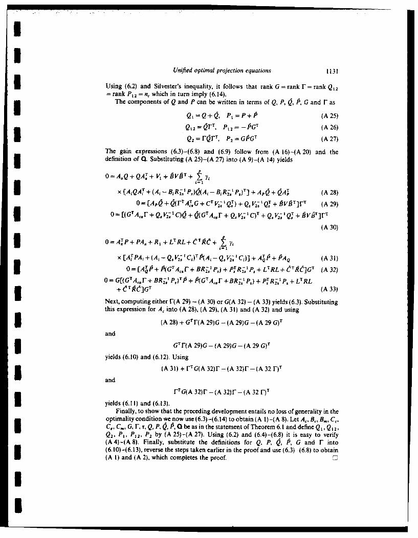
Unified optimal projection equations 1131

IUsing (6.2) and Silvester's inequality, it follows that rank G = rank F = rank Q12= rank P1 2 = nc which in turn imply (6.14).

The components of Q and P can be written in terms of Q, P, ,/A, G and F as

Q-=Q+O, P1=P+P (A25)

Q12 =O T, P1 2 = -15GT (A 26)Q2 =rr T, P2 =GPGT (A27)

The gain expressions (6.3)-(6.8) and (6.9) follow from (A 16)-(A 20) and thedefinition of Q. Substituting (A 25)-(A 27) into (A 9)-(A 14) yieldsO=A.Q+QA T+V+BVBT + V ,

x CA, QAT + (A, - BR - P5)Q(A, - BR -' P.)T] + Apo + A T (A 28)0 = [AO + (ITTA G , + C V2;I QT) + Q, V T +V ]FT (A 29)

0 =II(GA,. r + Q, V2;'cQ + (G A r+ Qv 21 C)+Qv 2 t+A v]r

(A 30)0 O= P+P A,+R,+LTRL+C ITiA + ,(

i= 1

x [Ar pA, +(A, 2;Q V1; Ct)TAA, - Q, V2' C,)] + AT 15+ PAQ (A 31)

0 = [ATP + P(GATF + BR-,' P,) + PTRZ-s'P, + LTRL+ CTR/]GT (A 32)G[(G'rA,. + BR2-t p,)r/i + 15(GA , Ba p) r- T

2s + Acr +BR2 P ) + PTR-' P, + LTRL+ CqfTI]Gr (A 33)

Next, computing either F(A 29) - (A 30) or G(A 32) - (A 33) yields (6.3). Substitutingthis expression for A, into (A 28), (A 29), (A 31) and (A 32) and using

(A 28) + GTF(A 29)G - (A 29)G - (A 29 G)T

and3 GTF(A 29)G - (A 29)G - (A 29 G)T

yields (6.10) and (6.12). Using

and (A 31) + FrTG(A 32)r-(A 32)r-(A 32 r)T

and

yields (6.11) and (6.13).rTG(A 32)r-(A 32)r-(A 32 )T

Finally, to show that the preceding development entails no loss of generality in theoptimality condition we now use (6.3)-(6.14) to obtain (A I)-(A 8). Let A,, B, B., C,,Ce, Cm, G, r, r, Q, P, Q, I, Q be as in the statement of Theorem 6.1 and define Q1, Q12,Q2, PI, PI2, P2 by (A 25)-(A 27). Using (6.2) and (6.4)-(6.8) it is easy to verify(A 4)-(A 8). Finally, substitute the definitions for Q, P, Q, ,. G and r into(6.10)-(6.13), reverse the steps taken earlier in the proof and use (6.3) -(6.8) to obtain(A 1) and (A 2), which completes the proof.

II

1132 'ifted opt vWi pVLAjet I ion eUqA 4I^

ALKMIT, ~.1969, SIAMf J APPI Aiduh, 17, 414BEaSm~i, D. S., IM1 a. I E f f Trdaj Juaiom Cmloa, . I b 196' b Isid 32. I I~Baa'.sma. D S. and HammAD, W M, 19"1 The Optimsi Piv giton t .datto Wit

Petenen-Hollot Bound% Robqnt Contioth Siththn sm ( eAIAWftta1l StaU.1tUa

Smabdaty Rtadius I E L E T'w'u mao G(Xm,. to br pubnhcaiBu~sniN.D S.,andHvrLA--t,D C. 4 9VA3LLtj%% Ta d,-A 30, (Iuk j 191b

Thwuf) y ppi. to be pJbihtdIBnawtaa, J W. 197& 1IfE f Tw 'wt: la S v a~,

GaLELEY. S W. and )HLAstD. D) C. 1913, KtdL4)tt0ct t.wnpwq&atioa 1L). ltcduvtl'wVerms, Opciama PVopwison)f -4 1 4 4 J btuJ (oLs tmt i tp bc otvplj~

HADDAD, W N4. W9,7 Robtisa op~maI piopmke contiov*ei'n ~ethw Ph DI 4iswttt

FLHADDAD. Wt M, and Da~sn% S, 198711 It tp" t'ai .m (wt, 2HYLAso, D C.. and Saa. rtI. D S. 1964, It 1. ftfm ?twa m ( c-me 29. 2Q14wb IS44

Josc~tuEm. EA.and Sitaw'.. L. %I , 98)11 ft I I Pat-da wtvXLV

Liu. Y. and ANDERsoN. B D 0. 196 .A u Couiwt4, 40 ~'RAD. C R.. a" MfTIA. S K, 1971. Gv.Ia~rJ lmewwiw a4 Uwra .i4 hi 4pfdu.sc*3 I%e'm

York: WlkyjRimta S. 1"17. Prar 4avwscam (mulo 'uJ wf. iwnc 19S' Uti'a'wape4n M%.WiLsoN. D A.. and Kt~siAl. A. 1")1. Pvrm I L I f (m oa Ow ingi 4 ( ,ims.o. tk~rnttw

19"3. San Antomo. TXWONNAM. W MI. 1979. LmnW'av 4Wuloug e rv d aw' 8 (,rIl1 4nywi4 Aff b 4-na Ipe

Verlag)

IAIPENMO 1: Fftut Syntheis~: QuadaticBon

I101. W. M. 11 mad D. S. Bobruuif, N"4*Ut, Cr ft"oft 1~siz via

U 3. W. N. II I a D. S. Biwtain, "Fbut Rmmd-tw MontrictlyPrwr State Extivtion via the aptim1 Projctioagwatiam with

with Patreik Ic ou~nds: Admo Stability and Peform viaIio-rerDwi fbr Sytem with Structure P3m-

I ~p. 578-M8, 11968.

113. D. S. 3mz~uteJi, 41obust Stability mun Pwfbnmnc via Piim-Or3Dyiic OMuuai-m SIAM J. Cotr. QgLIu., to apper.

692 MEE TRANSACTIONS ON4 AL~lMWATC CONThlOL. VOL 33' NO 7. iULY IOU

I of robust reduced-ortler estimation and comrcA in die preseace of real-valued. stactrd parameter uncenamyv This was accomplished bryvicorpor" iq mqadrati untaincutu pid~roposed ts 173 within Ccw

opualpo)ecUce frame'WorliTWI Proe 0( die Frer P - e is to complete this cycle of results by

silary etding the resilt of I I I. - a is o o&Awn robustreducad-oeder moels owe a specified rnge of parametnc plantoncenawy. Asa in 141-(61. the main idea is to bound the effect of theuncetan parameters on .me modei-redacton error over .me uncerwayrQng AMd thent determine a PI -ePd-orde, model which minimizes .memodel-raducuon bound The resulting generalization of .mw optimalprojection equatioins now serves as a Waffucteni condition for robust model

~a being munmizted rather than die model-reductiori error itself Theseaptialycodtions o* aeofgthe se ha a boud en o themdlreectloebraor

mainx equaont which reduce to the result Of I II when the uncertainqII bounds ame absent,

11 NOTAYON AND DIFPINrnoNKS

X3 5W". ql real numrbers. r x s real matrices. I'*l( ~ r rwiymetrtatntnpoe. expected value* Krosvlcker sum

5'.~ X' ' u r symmetric. nonn gative-defintite. posstive.definite maincesU, Z Z ' Z3 Zi- ZlN.2-ZeP'.Z.2 -E6

X. .yey. X..2 n. . 1,n.. 4-dieraonglictA.&A~..C n Xn matices. tx m.Ix n mancetA..B..C. ff. X mf..lX .In. matrces

R modelPIrefscio errnr-eh i x iatn Pw(- r-dimensional white r. -ict

RobstReucd-r M delngVi te ptma Intesiyof w()in P

Projection Equations with Petersen-Hollot Bounds ALCPR R.Rbs eue-rdrMdln i 9r cRC -CrRC.

3 WASSIM M HADDAD AND DENNIS S. BERNSTEIN FBVDT 3Bs1

Abstract-An otimal reducedorder .edellngprolik witliparsai. I B.VBT B. VBLJvie plant ateertalat) is eomuideredl. A mde4-eduirtiow hoed suggested III. ROBUST MODEL -RWUCL--ION Pitost-Ftll reent work of Petersen sad Hauntl Is utilized for guaraitelmg robasiI reduced-order modelingl over a specified mang of une~ert parameters. Uet 1A C X... denote the set of uncertain perturtions. &A of theNoessar) condiftIn which generalize the optimal projeciloa equatioa% nominal plant matrix A.fo. model rdtlon are ,, ed to chamrne h~e reducd-order mode Robust Mfodel-Reduction Problem; For fixed s. s determinewhich mialmizes the model-reduclion booed. The optlmaisp equatilows (A.. B.. C..) such thut, for the system consising of the nth-orderI thus effective) serve as sufficient eodloar for chasrocterlslag robust disturbed plantreduced-order models.

X(1) -(A + AA)x(f) +Bw(r). r E 10. co). (0.03IL INTRODUrCTION outpuits

It has been shown in) 1-13) that the first-order necessary conditions for yr X) 32quadrtcall, optimal reduced-orier modcling. estimation, and control ()-Crl.02can he transformed into coupled systems of two, three, and four matrx and n,.th-ordcr modelequations, respectively. This coupling is due to an oblique projectionwhich arises as a direct consequence of optimality. In a series of papers t(t) - A.x.Q) + B. w(t). (3.3)(4j-161 the optimal projection approach was generalized so the problem 34

Mtamacnpt received August 4. 1"?;~ rvised Ocober 16. 19117. Th& work ws the model-reduction criterionmPpnne to tan by the Aii t oe Oftie of Scmenfl Resue under C400rac F49620. -36-C-OW)Foiatiaiwo J(A.. B.. C.) 9 u lim sp J~y(t)-y..(t)ltrRl)(t)-,.tt)I

?.tmn*log. Melbourne. Pt 3MI0+DU S. Berm swt h oenetAmpc ysum isviminimized. (3.3)

CopiioMelbourne, FL 32902

001U-92WSSt/0700069S01.00 C Mg1 IEEE

IEE TRANSACTIONS ON AUTOMATIC CONTROL. VOL. 33. NO. 7 JULY ,Ia 693

For each reduced-order model (A., B.. C.,) and system variation &A Proposition 5. 1: The functionE %U. the augmented system (3.1)-(3.4) is given by 1

1(t). (A + AA)() + w), I E IO, co) (3.6) 0(.) 9 7, K4,D' 5+ Qr'rQ, (4)'-I

Where g() lQ xr (t) 1T. satisfies (4.3) with 11 given by (5.1). 1IV. SUFFICIENT CONDITIONS FOR ROBUST PERFORMANCE Proof- For i 1, . p,

The following result is immediate. INN

Lemma 4.1: Suppose A. is asymptotically stable and A + 1A is A M,MrTD!+ -N !N, 4,.-(IM,N,Ir, .+4 rN Mrbr)asymptotically stable for all AA E %. Then s ,6A , 1r+ qr?,.,0, -(,MN,,. + rTNT, MIrAr).

J(A.. B. C.)- sup ir ai.o1A (4.1) Summing over i yields (4.3). 0 3AC% Remark 5. 1: The bound (5.4) was originally used in 17) for unit-ran).

where 0.. j lir,_. I. 1 g(I).(t)r E iO is the unique solution to perturbations with scalar uncertain parameters. For further details, see141-161

0,-(A+AT)CA+0,A(A+A)T+ P. (4.2) 1

We now determine an upper bound for J given by (4.1) VI. THE AUXIIY MINIMIZATION PROBLEMTheorem 4. ." Lct 9:ff' -" Z' bc such that Our goal is to minimize the error bound (4 6).

Auxiliar)' Afinimizotion Problem: Determine (q. A., B., C.) withAA,4+4AAr5()., hA 6 'U1. 4 E Pjj (4.3) 4 E W which minimize

and. for given (A,. B,, C.), suppose there exists .E ' satisfying (., A.. B.. C.) G tr 4Qf (6.1)

)(4.4) subject to 3and suppose the pair (P'-. + &4) is stabilizable for all .14 E 91'.Then A. is asymptotically stable. A + A is asymptotically stable for all 0"-A +QAr+l; I ,,,+ Q[y,,Q.]+ P (6.2)AA ' . ". I

O,A s. &A E ', (4.3) and(P"f2. A+AAisst blizabe. AG 'I. (6.3)

where 0,A satisfies (4.2). and 1

Proposition 6.1: If(.., A,.. B,, C.) satisfy (6.2) and (6.3) with 4 z UJ(A,.. B.. C.)str q9. (4.6) 0. then A, is asymptotically stable. A + AA is asymptotically stable for

all AA E It. andProof See (51. 0

Remark 4. 1: Theorem 4. 1 provides sufficient conditions for reduced- J(A.. B., C.)< (L. A.. B.., C.). (6.4)order modeling with an upper bound on modeling error. The result yields. Proof- With 0 given by (5.4). Proposition 5.1 implies tt (4.3) isin addition, the result that A. and A + AA are asymptotically stable. saif with (6- 4). PoposiTo .1 p esatis.3eiThus. it is important to emphasize that our results are effectively limited satisfied Hence, with (6.3). the hypotheses of Theorem 4.I are satisfiedto systms which remain asymptotically stable over the class of so that the system (3.6) is stable over '11 with model-reduction oununcertainte. Relevant applications include, for example, damped flexi- (4.6) Note that with (6. (64) is merely a resttement of (4 6)blc structures with uncertain modal data.

VII. NECESSARY CONDITIONS FOR THE AUXILIARY MINIMIZATION

V. UNCERTAINTY STRUCTURE AND THE PETERSEN-HOLLOT BOUND PROBLEM 1Rigorous application of the Lagrange multiplier technique requires

The unccnaint) .et 'U i assumed to be of the form additional technical assumptions. Specifically. we further restrict (Q, A..C B,. C.) to the open set

11 AA. E ;?"":.AA D,(,N(E,,(M,4",sN!N,<s1,. 8 ; ((QA..4B.,C.) E P, 6 is asymptoically stable.

and (A., B.. C,.) is controllable and observable)I. 3 (5.1) where

where, for j = 1. ~,p:D, E 1' and EG E1" are fixed matrices (N 1 -denoting the structure of the uncertainty: M, E A', and N, J', are A+ f[ ,., A+ £rN.,, .given uncertainty bound%: and M, E ;t',", N, it'", arc uncertain / ,,- I,

matrices. The augmented system thus has structured uncertainty of the Remark 7.1: The constraint (4, A, B_ C,) E £ is not required forrobust reduced-order modeling since, as shown by Proposition 6. 1. only(6.2) and (6.3) are required. As will be seen from the proof of TheoremAA"). 1,M,N,R, (5.2) 7.1, the set $ constitutes sufficient conditions under which the Lagrange

• "multiplier technique is applicable to the auxiliary tinimizaton problem.

where Specifically, q. > 0 replaces . t 0 by an open set constraint. asyrmptoticstability of d serves as a normality condition which further implies that

J5 q [D .E A f 0.5.) the dual T~ of 4 is nonneptive definite, and (A,. ft., C.) minimal is a U0 , r, . [E, 01. (5.3) nondegeneracy condition.

The following factorization lemma is needed for the statement of the

We now specify the function 0 satisfying (4.3). main reault. For details, see (I

694 IEEE TRANSACTIONS ON AUTOMATIC CONTROL. VOL. 33. NO 7. JULY 1969

Lemma 7.1: If 12, P e i and rank QP - n.. then there exist n. x VIII. SUFFICIENT CONDITIONS FOR ROBUsT REDUCED-OIDERn G, r, and n. x n., invertible M such that MODEUNG

G .CTmr, (7.1) The main result guaranteeing robust model reduction can now beI stated.por-/... (7.2) Theorem 8.1: Suppose there exist Q, 0., P E @I satisfying (7.8)-

(7.il)and suppose that (P"2,A + AA) is stabilizable for al &A E 'IFurthermore. , , M.and r are unique except for a change of basis in '-m. wihABCgveby(.-77)ad1 efndy(51.Ten.RealfrmI1 htwith A.,, B., C. given by (7.S)-(7.7) and 'Lt defined b (5.1). Then A.,

Recall from Is that i asymptotically stable, A + AA is asymptotically stable for all AA E

r A OP(0P)'-Grr (7.3) U, and the model-reduction criterion satisfies the bound

is an oblique projection, where( )' denotes group generalized inverse. J(A B.. C.)s tr QCrRC. (8.1)Define the complementary projection 7, 1., - r and call (G, M, r) Proof: The converse of Theorem 7.1 implies that Q given by (7.4) issatisfying (7.1). (7.2) a projective factorization of OP. Furthermore, nonnegative definite and satisfies (6.2). With the stabilizability assump-define the notation tion the result follows from Proposition 6.1. C

D DALDI. E E[RE,. Remark 8.1. As noted in Remark 4.1. Theorem 8.1 is effectivelylimited to systems which remain asymptotically stable over the class ofuncertainties.

Theorem 7.1: Suppose (4. A,,, B,,, Cm) E 8 solves the auxiliaryminimization problem with 'U given by (5.1). Then there exist Q, Q, P E APPENDIXN ' such that Q, A., B.,, Cm are given by 1PROOF OF THEOREm 7.1

ro rorr , (7.4) To optimize (6.1) over the open set

A.='(A +QE)G r, (7.5) 8' Q {(. A.. B., C.) E S : (6.3) is satisfied}

B. = rB, (7.6) subject to the constraint (6.2), form the Lagrangian

C.,=COT (7.7) 2 (A., B.. C,4.( )

for some projective factorization (G, M. r) of QP, and such that Q. Q, P t, ,b + iic,,T, ) , .*satisfy V ~ ~ b%, tN~+~J(j

O =AQ+QAr+D+QEQ+T.BV~ri, (7.8) where the Lagrange multipliers X 0 0and6 E ft'are not bot zero.0=(A + QE)io+ (A+QE)r+.E1+BVBr- 7BVBrr r , (7.9) We thus obtain

0=(A + QE)TP+P(A + QE)+C TRC- ,r CTRCT.,, (7.10) 8. A T .A+(p,, ++-R.. 4 E~.6 +rtpm +~l x.+ ,4

rank Q=rank P= rank oP=n.. (7.11)

3 Furthermore. the auxiliary cost is given by Setting 8.2/8 - 0 yields

Conversely. if Q, (, A E 11J1 satisfy (7.8)-(7.1l) then (4, A,,, B,, C,) where "vec" is the column-stacking operation (see 161). Since 6 isgiven by (7.4)-(7.71 satisfy 4 _ 0 and (6.2) with auxiliary cost given by assumed to be stable. d T is invertible, and thus X = 0 implies (P = 0.(7.12). Hence, it can be assumed without loss of generality that X I.

Proof See the Appendix. C Furthermore. the stability of a r implies that (P is nonnegative definite.Theorem 7.1 presents necessary conditions for the auxiliary minimiza- Now partition A x h Q. (P into n x n. n x n., and n. x n.

tion problem which explicitly characterize extremals (Q, A. B,,, C,). subblocks asThese necessary conditions consist of a system of two modified Lyapunovequations and one modified Riccati equation coupled by an oblique Q,. ] P, P1.]projection r and uncertainty terms. Setting D and E to zero. i.e., deleting , = 1 2the plant uncertainties, it can be seen that (7.8) drops out while (7.9) and Q z 1P,2 PQ

(7. 10) reduce to the optimal projection equations for model reduction Thus, the stationarity conditions are given byobtained in IlI. If. alternatively. nm = n, then the full-order robust modelis given by A + QE. B. C where Q is given by (7.8) with 7, = 0.

Remark 7.2: As in the perfect modeling case considered in 111, (7.8)- _A(P +(6A + (A.2)(7.10) may support multiple solutions. When uncertainty is present but a G4 , 'full-order model is desired, then the solution is unique.

Remark 7.3: The conservatism of the bound (7.12) is difficult to 8predict for two reasons. First, the overbounding (4.3) holds with respect TA. 2Qp 2 +p 2Q=0, (A.3)to the partial ordering of the nonnegative-definite matrices for which noscalar measure of conservatism is available. And, second, the bound (4.3) BV(is required to hold for all nonnegative-definite matrices 4. The 'BT, BV+P2B,,V,, (A.)

conservatism will thus depend upon the actual value of 4 determined bysolving (6.2). Numerical experience with related bounds shows that the i-g= -RCQ,2+RCQ2,0. (A.5)conservatism is highly problem dependent. See 181. BC.

IEEE TRANSACTIONS ON AUTOMATIC CONTROL. VOL. 33. NO. 7. JULY 1988 695

Expanding i(6.2) and (A.2) yields Defect Correction Methods for the Solution of Algebraic 30=AQ + ,A + D+QE. +BlI~, (.6)Riccati Equations

0=AQi2+Q,2A.I+QIEQI+BVBEr. (A.7) V. MEHRMANN AND E. TAN3

0-A_.,+2A.TQ7E,2+.VB., (.8) Abstract-The solution of discrete and continuous algebraic Riccati0A.Q+QAT Q~~i+L BT1(S equations Is considered. It bs shown that If an approximate solution is

obtained, then the defect for this solution again solves an algebraic30=ATPl+PA+E(PIQI+P 1 ,QI )r+(pQI+P2Q,2 )E+CrRC, Riccati equation of the same form and that the system properties of

(A.9) detectability and stabliabllity are Inherited by this defect equation. Onthe basis of these results. a general defect correction method is proposed

0 = 'Pl+ P1A. E~p Q,+ p2T CR~m. (A.10)and numerical examples are given for the use of (his method in0=A~+iaA,+(P~I 2 Q .r, R'. AO combination with the SRt method.5

0 'P 2,+CrC.(All1) 1. INTRODUCTION

Now define the n X n nonnegative-definitc matrices We consider the numerical solution of generalized algebraic Riccaiequation%

Q Q'~i:Q'Q,, P~g p r P O=AOXE+ E*XA -(BOXE+ S)*R- (B*XE+ S*)+ C*QC=eIR(X)

Q0= EXE +A XA (A*XB + S(R 4 BXB)i -I

and the nt,, x n. nx n.,~ n. xIt matrices . 4AX8+S)*C*QC=Dc1X) 0.2)

12;Q, ~ r= P-P, R* E 0a".m are positive definite and E is nonsingular. Both equatin Ianse. for example. in the solutions of linear quadratic optimal control

* The existence of Q, 'and P -'follows from the fact that (A_,. B_, C',,) is problems. Equation (1. I) stems from a continuous-time and (1.2) from a* minimal. See J111-141. 161 for details, discrete-time problem (see, e.g.. 111, [4). and 151). The numerical 3

Note that (A.3) implies (7.1) and (7.2). Sylvester's inequality yields solution of these two equations has been studied extensively in recent(7.11). Next (7.4). (7.6), and (7.7) follow from the definition of Q, years (e.g.. [71, [41-161, [91, 1141, 1161, 1171. and 1201). Typically.relations (A.4) and (A.5). and dhe identities solutions are obtained using QR- or QZ-type algorithms to compute

deflating subspaces of the matrix pencils

Q, =Q + Q Q2z= Qr". P12 ., Qr. PGPG T. A 0 B] [E 0 01Computing either r(A.71. (A.8) or G(A. 10) + tAll1) yields (7.5). [C *Q A* SR - 0 0E 0, 13

* Inserting 07.5-(7.7) into (A.6)-(A. 11) it can be shown that (A.8). (A.9), L J0* and (AllI) arc superfluous. Using (A.6) + GrA.7)G - (A.7)G - corsndgtopblm( Dad

[(A 7)GI I and G Tr(A.7)G - tA.7)G - l(A.7)G IT yield (7.8) and crepnigt rbe 11 n(7.9). Similarl). r7 GtA. Iou' - (A. 1)1 - I(A. I011'] T yields (7. 10). [A 0O B1 [E 0 0

Flnall%. the proof can be reversed so that (7.5)-(7.11) yield (Al)D- jC*QC PE S ~ 0 -A* 0 (1.4)(A. 5 and (6.2). [S 0R10 - 0 J

corresponding to problem (1.2). where, using the fact that R is positiveREf-RNCT.S dec ite. man) of thc algorithms are applied to the reduced pencils.

ill 1) C lHl..nd ind D) S Bern..iein.."he optna prieto eqain fo [tjc FE G0 [reduoi.'n and tht rclaionship among the meihovi, .l Wi-n. Skelion. and [H -F J [ JN11,r. 1FF! Trani. .lAurorati. voiar.. vol AC-10. pp 1201-1211. 19815r

PI D) S BL rn~ctn and 1) C HN land. "The optimal Projcion equations for redu..d. I A - BR IS- BR - I& [E 0,'rdcr viii, cstitiio.n." IEEE Tram...Iiointat Conrar , %ol AC-30. pp 583- LCQ-R '~ - 5 +R 8

13 ) .Hij~ and D) S. Btern~icin. "The optimal projcdion cquat")n% lor livo E (S4 mdcr dlninitc conlpensatinn.- IEEE Transi. Atortat, Conhr.. vo,). AC 24. pp. corresponding to (0.3) and* ~10.14- 10137. tn4 r

141 W MI Haddid and 1) S Blernstein. "Robust. reduced~irder. nonsiril propr F 0 [E -Gstale estimatin ia the opitinisl proiccttoni equatio*n, with Ptrbcs-Hollot Hf Es ' 0 F*hiound,.- Sea: Con:,r. Lett,. vol Y.~ pp, 421-431. 1997L J L I

131 1) .1 Brrteoin and W MI Haddad. -The opoimral protction equation,. withPeter.itn Holloil Bounds R,.husi siahilits And perforiiwe via fixed-tinier [ A -BR IS 0 E - BR -5N-. 16

tion,." IEEE Trans. Airiomia, Conir.. vol 31, pp. 578-582. 1988. i161 D S Bems~tit and W M Htaddadj. "The optimal projection equations with corresponding to (1.4).

Petrrsen-Holl'4 bound'. Robust controiller synthesi% with guaramsed structuredstabitirq rwduu.' in Proc. IEEE Conf. Decison Comm,.. Los Angeles. CA. Dec1917. pp 1308- 1318. Manuscripit received February 13, 1987. revised September 28. I987 Paper I

* 171 1I.t Petersen andI C. V. Hotllot. 'A Riccata equation approach i the stAbiation recommended by Associate Editor, B. H. Krolh.of uncertain systems. " A ufomauica. vol. 22. pp 397-411, 1986. The authors are with the Fakultat lr Mathemnafii. Universilal Bielefeld. Bielefeld.

Ill D S. Bernstein and W M. Haddad. 'Robust stability and perfoinmance analysih Wesl Germany.for linear dynamnic systems." submitted for publications. IEEE Log Number 8821013.

0018-9286/88/0700-0695S01.00 @ 19881IEEE

i Systems & Control Letters 9 (1987) 423-431 423North-Holland

Robust, reduced-order, nonstrictly proper stateI estimation via the optimal projection equations

with Petersen-Hollot bounds

Wassim M. HADDAD

Department of Mechanical Engineering, Florida Institute of Technoloy. Melbourne, F 32901. USA

3 iDennis S. BERNSTEIN *Harris Corporation, Government Aerospace Systems Division. MS 22/4848. Melbourne. FL 32902. USA

Received 10 March 1987

Revised 11 June 1987

Abstract: A state-estimation design problem involving parametric plant uncertainties is considered. An error bound suggested by3 recent work of Petersen and Hollot is utilized for guaranteeing robust estimation. Necessary conditions which generalize the optimalprojection equations for reduced-order state estimation are used to characterize the estimator which minimizes the error bound. Thedesign equations thus effectively serve as sufficient conditions for synthesizing robust estimators. An additional feature is thepresence of a static estimation gain in conjunction with the dynamic (Kalman) estimator, i.e.. a nonstrictly proper estimator.

Kevywords: Robust Kalman filter. Error bounds, Reduced-order state estimation.

1. Introduction

As is well known (2,5-8,11,14,151 optimal filters based upon nominal parameter values may be severelydegraded in the presence of parameter deviations. Thus, it is desirable to obtain robust state estimatorswhich provide acceptable performance over the range of parametric uncertainty. The approach of thepresent paper is related to the guaranteed cost approach developed for control in [4,161 and applied toestimation in [11]. Specifically, the main idea is to bound the effect of the uncertain parameters on theestimation error over the uncertainty range and then choose estimator gains to minimize the estimationbound. Thus the actual estimation error is guaranteed to lie below the prescribed upper bound.

The technique used to determine minimizing estimator gains is based upon a generalization of theoptimal projection equations for reduced-order state estimation [1]. Thus the results of the present papereffectively extend the results of [1] to the case of system uncertainties. It should be noted that the optimalprojection equations, which are necessary conditions for optimality, now serve as sufficient conditions forrobust estimation by virtue of the fact that a bound on the estimation error is being minimized rather thanthe estimation error itself. The bound utilized in the present paper is an extension of the approachdeveloped in [12,131 for constructing Lyapunov functions for full-state feedback and utilized in [10] tocharacterize the structured stability radius.

An additional feature of the present paper is the inclusion of a static feedback gain in conjunction withthe dynamic estimator. Thus the results of the present paper represent a generalization of standard resultsto the case of nonstrictly proper estimation.

* Supported in part by the Air Force Office of Scientific Research under contract F49620-86-C-0002.

0167-6911/87/$3.50 " 1987. Elsevier Science Publishers B.V. (North-Holland)

I

I424 W.M. Haddad, D.S. Bernstein / Robust estimation via optimal projection equations

2. Notation and definitions

Note: All matrices have real entries.R, R×S, Rr, E real numbers, r x s real matrices, R' × , expected value.I" ( )T r X r identity matrix, transposeSr, Nr, Pr r x r symmetric, nonnegative-definite, positive-definite matrices.Z<Z, Z, <Z 2 Z 2 - ZI- N, Z2 - Z Epr Z , Z 2 E Sr.n, I n e, p, q; h positive integers; n + n .x, y, y , ye, x.,x n, 1, 1, q. ne, f-dimensional vectors.A, AA; C, AC nXn matrices; /Xn matrices.C, L, R t Xn matrix, q x n matrix, q Xq matrix, R C P,A,, B, C, D, n Xn. n X, q X n., X I matrices. 3. ,, [ A 0 - [ AA 01 IRBC A B't, a

[LTRL - LRDe(C TDTRL+CTDTRD2(f LTRC,+ CTDTRC]

[ - CT RL + CTRDf CrTR C,wo(.), w(.) n, -dimensional white noise.Vo . V intensity of wo(.), wl(-); V-N", V GP'.

Vo n X I cross intensity of w"(I), W "().Wo(') 1 [ V0 Ovo0 OB: 1' w ( IV) W [ O(-)/ " 'Tv oV., B :](~~w( B] L e01 Be VB

3. Robust estimation problem

Let a'c R" ×" x R'/ " denote the set of uncertain perturbations (,IA. AC) of the nominal plant matrices Aand C.

Robust Estimation Problem. For fixed n, 5 n, determine (Ac, B. C , D,) such that, for the system 3consisting of the n-th-order disturbed plant

i(t)=(A+AA)x(t)+wo(t), tG[O. oc), (3.1)

noisy and nonnoisy measurements

)(I) = (C + AC)x(t) + w,(t), (3.2)

I(t) = Cx(t), (3.3)

and n,-th-order nonstrictly proper state estimator

i,(t) = A,, (t) + Bey(t ) , (3.4)

y(t) = Cexe(t) + DeJ(t) , (3.5)

the state-estimation error criterion 3J(A,. Be. Cc. De) sup lim supE[ Lx(t) -y(t)IT R[Lx(t) -y,(t)] (3.6)

is minimized. 3Note that the augmented systen (3.1)-(3.5) can be written as

X (t) ,+AA t+ 0(t), t C[O1, X), (3.7)

where .C(t) [ [xT(t), xT(t)] r. The cost can be expressed in terms of the augmented second-moment matrix.

I

i I

UW M. Haddaj4 D. S. Bernstein / Robusst estimation via optimal Projection equations 425

Proposition 3. 1. For given (At, B~, C, D,) and (A A, AC) rE '& the second-moment matrix

satisfies

Furthermore,UJ(Ae, B., C, D )= sup lim sup trQ,(t. (3.10)

4. Sufficient conditions for robust performance

Lemma 41.Suppose the system (3.7) is stable for all (AdA, AC) E qIr Then

J(Ae, BeC.,DJ) sup trQ.,R (4.1)(IA. .IC)e91

where I E N'1 is the unique solution to

I We now seek upper bounds for J(A,. B,, C., Dj)

Theorem 4.1. Let Q2:N x R n- x 1 - S be such that

dJU- AA+ 9 ~ (.2, Be), (A A. AC)eq/-,, (.2, Bt)GN i-x R lx , (4.3)

and. for given (A., B., C,. D,), suppose there exists .2 E- V' satisfying

0 = 4 + .2ATT+ 2(2,. Be) + V., (4.4)

and suppose the pair iV12 +44A) is detectable for all (,I A. AC) c- qI. Then A,, is asvmptoticallv stable,3 A +d A is asymptotically stable for all ( AA, AC) E '-

where 0., satisfies (4.2), andIJ(Ae, Be, C, D):5tr.R. (4.6)

Proof. For all (A A, AC) E LIZ, (4.4) is equivalent to

whereq'2 B, A ) =12 .,B. -(3 A2 +21 T .

Note that by (4.3), kI(.9, B~, 14);_>0 for all (,IA. AC) CE '. Since (91,2, ' +'34) is detectable for all(AA, AC) eeV, it follows from Theorem 3.6 of [171 that ((17+ 'I'(.9 B, AiA))' 2, + Ai) is detectablefor all (A A, AC) E= I. Hence Lemma 12.2 of [ 17] implies i + Ai is asymptotically stable for all(AA. AC) e V'. Since i + AA is lower block triangular, A. is asymptotically stable and A +'AA isasymptotically stable for all (A A. AC) e *t. Next, substracting (4.2) from (4.7) yields

0+ (.9- 4i+'di) T + *'(_Q. B'. 'i),

426 WM. Hadda4 D.S. Bernstein / Robust estimation via optimal projection equations 3or, equivalently, (since A + AA is asymptotically stable)

2 - =.di -- e i+4( , Be, Ai) e(A+Ai)T dt >_ 0,

which implies (4.5). Finally, (4.5) and (4.1) yield (4.6). 0 35. Uncertainty structure 3

The uncertainty set Tk is assumed to be of the form

pqz= {(AA, AC) r Rnx× X R'x": AA = . D,MN,E,,

i-I1

, NNE,, M,M, <M,, N, TN< ,= .p}, (51)

where, for i = 1,..., p, Di e R" × ', E e R ''," and F, E Rx r, are fixed matrices denoting the structure of 3the uncertainty; M, re N ', and N,r N' are given uncertainty bounds; and Mi, Rs , N ER R' areuncertain matrices. The closed-loop system thus has structured uncertainty of the form

di ,M,NE,, (5.2)i-1

where 3hA [D' j'A 01. (5.3)B,= BF,"

The special case -=I, ,; N, I,, is worth noting.

Proposition 5.1. Let i, v > 0, i= 1....p. Then M,M,T5gI and NTN 2 J_ if and only fIomax(M,) < At, and omax(N,) < V,.

Remark_5.1. qI given by (5.1) is directly related to the structured stability radius introduced in 110). Setting 3p - 1, M 1 =pL,, r, --s, N = I,, and N, = I,, yields the setting of [10]. For a similar formulation, see(131.

6. The Petersen-Hollot bound

Given TI as defined in (5.1), we now specify 92 satisfying (4.3). 1Proposition 6.1. The bound A? given by 3

p

j2(ReB) AE b, R,15 + ,r,Ti. (6.1)i-I I

satisfies (4.3) with Vit given by (5.1).

II

I

I W.M. Haddad, D.S. Bernstein / Robust estimation via optimal projection equations 427

Proof. For i =1...,

0.:5 [bA. 2TNT 1bM, .qt NT IT

- bM, M7D +.2T,r , -(b, N, 2 . 2~, i TM~bI)

<5 b,'b , +.2ATi,.9 - (b,M,N, 2 +2 T NT M,Wb ).

I Summing over i yields (4.3). U3

Remark 6.1. The bound (6.1) is used in [121 for unit-rank perturbations while a more general treatmentappears in [131.

7. The auxiliary minimization problem

3 Our goal is to minimize the error bound (4.6).

Auxiliary Minimization Problem. Determine (.9, A.. Be, C. D,) with _q G N which minimizes

,,f(.2, A, Be, Ce, D,) A tr 2 A (7.1)

subject to'i2 + 2A4" + E [/b,R, b, +.2,TRL',-2 ] + P. (7.2)

i-1

I anda d (171/2, i + 44) is detectable, (d A, dC) r zl (7.3)

Proposition 7.1. If (.2, A , Be, Ce, De) satisfies (7.2) and (7.3) with .2 0, then 4 + A is asymptoticallystable for all (A A, AC) e 1, and

J(Ae. Be, Ce. De) (.-2, Ae, Be, C, De). (7.4)

Proof. With S2 given by (6.1), (7.2) is equivalent to (4.4). Hence. with (7.3), the hypotheses of Theorem 4.1are satisfied so that the augmented system is stable over q with estimation bound (4.6). Note that with1 (7.1), (7.4) is merely a restatement of (4.6). 0

8. Necessary conditions for the auxiliary minimization problem

Rigorous application of the Lagrange multiplier technique requires additional technical assumptions.

Specifically, we further restrict (.2, Ae, Be, Ce, D,) to the set

YA {(., A4, Be, Ce. Do): 2r P'1 , .2? is asymptotically stable. (Ae. Be, Ce) is controllable

and observable, and C(Q - Q1 2Q,-Q2) C r> 0},3 where ( 9 denotes Kronecker sum [3])

and .2 is partitioned as in Appendix A. As shown in Appendix A, Q2 is invertible since (Ae , Be) iscontrollable. The positive definiteness condition holds when C has full row rank and .2 is positive definite.I

I

I

428 W. M. Hadda4 D. S. Bernstein / Robust estimation via optimal projection equations

As can be seen from the proof of Theorem 8.1 in Appendix A, this condition implies the existence of theprojection T' defined below. Note that 9Y is open. 3Remark 8.1. The constraint (2, A €, Be, C, D:) (=- is not required for robust estimation. As will be seenfrom the proof of Theorem 8.1, the set Y' constitutes sufficient conditions under which the Lagrangemultiplier technique is applicable to the Auxiliary Minimization Problem. Specifically, asymptotic stability Iof Q? serves as a normality condition which further implies that the dual 9 of .2 satisfying (A.2) isnonnegative definite. Furthermore, (Ae, B , C,) minimal is a nondegeneracy condition which implies thatthe lower right ne x ne subblocks of ,2 and 9 are positive definite. It is extremely important to emphasizethat Proposition 7.1 shows that it is not necessary for guaranteed robust estimation that an admissiblequadruple obtained by solving the necessary conditions actually be shown to be an element of Y'.

For arbitrary Q - Rnx" define the following notation: 3p p

Vi I+EFj'T 1 Q i+ QC T + D, W FT.

p p AD A E DiD7, E:& E E7NE,, A A - QaV'C.

i-I 1-I

The following factorization lemma is needed for the statement of the main result. See [11 for details.

Lemma 8.1. If Q, P C N" and rank QP = ne, then there exist n, X n G, F and n, X n, invertible M suchthatI

t & = GTMr, rGT= 4.. (8.1),(8.2)

Furthermore, G, M and F are unique except for a change of basis in Rn'. ISince &I is diagonalizable it has a group generalized inverse (Q )= TGM- 1F and

-_ 4P(P) " = GT F (8.3)

is an oblique projection. Define the complementary projection T, A1 4 - T and call (G, M, F) satisfying(8.1) and (8.2) a projective factorization of QP.

Tieorem 8.1. (.,, A. Be, Ce, De) EA 9 is an extremal of the Auxiliary Minimization problem with q1 given 1by (5.1) if and only if there exist Q, E, s N" such that .2, A. B , C , D, are given by

Q+Q rQFT (8.4)

Ae = F(A- QV.'C + QE) G (8.5)

Be =FQVa, (8.6) 3C, = LT1 GT, (8.7)

D, = LQeT(eQeT)-, (8.8) 3for some projective factorization (G, M, F) of OA and such that Q. Q, P satisfyOQ QAT+VoD QQ - Q " -jI Q;T

o-AQ + V0 + D + QEQ - QaVj'Qa + T 'QTViTQ-I, (8.9)

0 (A +QE)Q+ Q(A + QE)'+ QEQ+ i (8.10)

0=(AQ+QE)Tp +P(AQ+QE)+rT LTRL - T T T T, LTRLTl, (811)

rank Q = rank P = rank QP = ne, (8.12)

II

IWm. Hadda,4 D.S. Bernstein / Robust estimaijon via optimal projection equations 429

where

I A'1 QCT(CQfT) - I, T, In- T'. (8.13)

Theorem 8.1 (proved in Appendix A) presents necessary conditions for the Auxiliary MinimizationProblem which explicitly characterize extremals (.2. Ae. Be, Ce, D,). These necessary conditions consist ofa system of two modified Lyapunov equations and one modified Riccati equation coupled by two obliqueprojections T and T, and uncertainty terms. The projections r and T correspond to reduced estimatororder and singular observation noise, respectively.

Several special cases can immediately be discerned. For example, in the full-order estimator case n. = n,set T= , so that T, =0. Now the last term in each of (8.9)-(8.11) can be deleted and G and F in(8.4)-(8.7) can be taken to be the identity. Furthermore, since Q and P now play no role in determiningthe optimal estimator, equations (8.10) and (8.11) are superfluous. If. furthermore. D, E, and F, are zero.then (8.9) reduces to the standard observer Riccati equation of steady-state Kalman filter theory.Alternatively, the case in which the static estimator gain D, is absent can be handled by ignoring (8.8) andsetting r = 0. If, furthermore, the uncertainty terms are deleted then the results of [II are recovered.

9. Sufficient conditions for robust, reduced-order estimation

The main result guaranteeing robust estimation can now be stated.

Theorem 9.1. Suppose there exist Q, Q, P I N' satisfying (8.9)-(8.12). let Ae. Be, Ce, D, be given by(8.5)-(8.8), and suppose that( 1 1/ 2, A + Ai) is detectable for all (A A. AC) E I& with Vj given by (5.1). ThenA, is asymptotically stable, A + A A is asymptotically stable for all (A A. AC) E V/. and the estimation errorsatisfies the bound

SJ(A. BCe. De) < tr QTrlLTRLr*I. (9.1)

Proof. Theorem 8.1 implies ., given by (8.4) satisfies (7.2). With the detectability assumption the result3 follows from Proposition 7.1. 0

Remark 9.1. Note that if C = L then Ce = 0 and the estimation bound (9.1) is zero since Ce1 T 0. This is.of course, to be expected since perfect estimation is achievable in this case.

Remark 9.2. The problem of designing reduced-order, robust estimators for unstable systems remains anarea for future research.

U Appendix A: Proof of Theorem 8.1

Partition i Xi ., 9 into n x n, n X n., and n, × n, subblocks as

-.2=[O 0] "= [Pr P2]

and define the n x n nonnegative-definite matrices

, Q 12Q Q T p A p, - p T

2 1 - 12 . 12"3 QQ12Q)2 1 ,1

The existence of Q2 ' and P ' is shown below.

II

I430 W. M. Haddad, D. S. Bernstein / Robust estimation via optimal projection equations 3

To optimize (7.1) over the open set 9"', where Y' A {(2, A:, B. Ce. D,) E Y: (7.3) is satisfied).subject to the constraint (7.2), form the Lagrangian 1

Y(.9, Ae, B , C', D.) & tr[X-9 (A-9+ -r + .fT+ P-,SN fT, + T):

where the multipliers X > 0 and 9 E RAn' are not both zero. We thus obtain

U - A 2 +_ + +rE L 2 2 9 + .

Setting 3.. = 0 yields ('vec' is defined in [31)jZT vec 9= - Xvec R.

Since 2? is assumed to be invertible, X = 0 implies 9= 0. Hence, without loss of generality, set X - 1.Since, furthermore, 2 is assumed to be asymptotically stable, 9 is nonnegative definite. The stationarityconditions are given by rI

pT----9 +Ar + 2 f TffN, 2 + l7=0o, (A.1)

4 +K 94++t , + A o. (A.2)

7= P 12QI + P2Q2 =0 , (A.3)

~'=pr, 0 , + (p Q, + pQT)CT + P 2 Bell,=0. (A.4) 3. = RLQ 12 + RDeCQ 1, + RCeQ, = 0. (A.5)aY - If T CT T=0

=7D RLQCT + RDCQC T + RCQ2,CT . (A.6)

Expanding (A.1) and (A.2) yields

0 =AQ + Q.A T + D + QEQ, + Vo , (A.7)

0 = AQ 12 + QICTB T + Q12AT + Q, EQ12 + voI Be. (A.8) 30 = eBCQi, + AeQ 2 + O12CTB + Q,AC + BCVIdB + Q , EQ1 . , (A.9)

0=P12 A, + ATP 1, + CTBP, + E( 1 1pQ2 )T- LTRC DRC (A. 10)

0= P2 Ae + AlP, + CTRC. (A.ll)

Note that the (1.1) subblock of equation (A.2) characterizing P, has been omitted from the aboveequations since the estimator gains are independent of P,. Writing (A.9) as (see [1.9])

0 = (Ae + BCCQIQ " )Q2 + Q2( Ae + B:CQ1Q- ) + Q2(Ql2QZ )EQIQ1.Q, + B..'IJBe

where Q.* is the Moore-Penrose or Drazin generalized inverse of Q2,. it follows from [17], Lemmas 2.1 Iand 12.2. that Q2 is positive definite. Similarly, (A.] 1) implies that P is positive definite.

Next (8.4), (8.6)-(8.8) follow from the definition of .2. (A.4)-(A.6) by using the identities

Q1 =Q+Q. P, =P+ P, Q 1,,=OfT , P,=- G r. Q2=Arr. P,=GPG. III

3. ~ ~~~~~W lMiS 0"& D va ,D., &Pm j.....r'

CoMputing other 1'(AS)-( A 9) oG AL k-Al l)~.t cli ~ twui 6 t I,&Iic-t~~t i ititoA Ok'iA IIIad usiflg(A.7) +G Ir(A.8) - (A S)G -(IA 9,G' &J GI f hA ISi 4 Ait OG 4 A G *arlj' 1 ) t i ? 10 1

Similarly, rFTG(A. i0)r - tA 10)1' - (A 101') t .ckh S1II.

Finally, the proo( can be rei',cd w thAt~ 4 b5p 4 121 .i IJA10 k f ,.U4i t' I SC 1911 uIIVJA

[1) DS. Bernstein &Md VC H ,La" ftho vi~ pomotf 1, '%a' J1 I woA'I Cioajpd 30 119, 5) 53(21 S.P Bh..cghani. Thor strwoutou' -1 tbait III I t'w,o 1#1 k .~IS b~ l t

(31 1.W Bw,c"w Ksoiw.k* puda t and o4ain , '_o". "&~a ,II t.*. -. *.

141 S.S.L, Chaag and TK C Pwt AJi'.a~oi sooujahd 4VAkt I *AVA It 44k~~ JI I I Oi'fooudI C~,g'o/ 17t92 474 -49 1(51 RtC Chun$ an P9. btfoinge %fan~ms j*bttv fhor v , Wwsg -.- o ' v '8£ , 4.*t£I

ten. IEEE rT'.u 4auumu it oupoi li 1Y* VPf O

161 )A. D*App btu and C I t~ aha. Lvo mommuttv saI~o ,- maw t r~h. "" .I *,£ p-to3 unceruantnza. IEEE T'umt 4wu,~wa Comtov4 it" 1,)t Wi171 T E Dyalms. Robust Obngi liV oololff-s UtLb PWSM~ta S* ftooo:' L4' 1%&

181 K Fiinata S Hats and 5 M.ort, A d...a oA ovba v'th amo % 'Ot~r lift ?'a,*: w,..i ~ 1

191I W M. Haddad, Robust (ptmnitl "sum. ft t*)ia ~£ hm w', i 4~au.~ m.i~I ~ ~~~~in&. Fovida laitto of Teohavk* 4jmu. L'Lat 10 mnhw adAJPths. aboun t' ti Lft m'tuaq b I 4pw*£m g'~ewis

Coortri Left 8 19I7 W 10 - I I)[111 SN Im ft. Guantowad f10 t~f) ,*I it~om I~&f v f~ W~w ag. Iw 3 7.

[131 1 R ft tennan A *'a'L"x H. pvk* ftjqIIazs quaama- omfovta !., .~aw aa odm $Aw ' lo m4wt IW~'m i V

ILmt, 25190)115- 1(11A.V nerAM L~mm J wi k- t.1d (tno " neei ov woit. 4 a4-f v'11.%a. -1 *,I 1,"vvw

I17)49-5U11WNIWfh~'LnwS'

3 *g*WU TRAJs$ACTIOLWS Ok AL!WiMflC COTRm~th %'t. S3 No 6 1UI4 I%"

1.000 beal so"ue bj % e "to a of Peew.r a" 140 i"dedi golwimue am* *0 sowma..d ce" opsubaf of (bg MeW

toa sopee - ub") otib rob"u OWGCIaMaac basedNewmann Cooutom usb" imst p diuese -pw pqooma gssI~o leePeedaee mmmk coretonaam weind go Cbaevto ofe

u~b - abe baedw Tiler Oamagu .guaahm160 tiflftliliel Un mo .gtfhr*e toodwe" for "bees dyinmar

At ns toU &Lw's. IQII mod LQG wufiri L.A j

soe~rtill five"i W~ affbdta% pawrametrwt~ulo~I 1:1 T*W* it10 not Wi#Pns*A " ire at,~ CUIVaalees r M i an the itftb utt andsymiirw of kv4*ae, ctwt%&ers uka't aft rabusa s ath respect to

woted so paehurd tK th OuratteWiL itu* oath N~eni ate (,A

an -~ 14 pamAIb the 64M ailetkdm ot ,t eperm0 a o hi

bowd. Prtent. ando"to1 1ak ma 171l~ coiadt a different "tfisr"e ftcatifwoon shich uiiLsw a qwudrasa Lymasnm bound to peato robutW3*sls) eee a trag ofsn0 Pllalabnt varsatoaww Ii the giamw paper.ug ce 9 pesotib o( botlm of iese appromachet to *btas both robit

Racca. and patIonad temn~w lersLauo.euaanhc

TOw erekremir ft sblay anti erformanc ver ducorde bountrl)s

protqe by Ch W rl iuna pn i the efrac fcnrleso atq dfomer oThe erformae und a' the uwrplareic w&sas the t entoa fos nWe~b, m0rnm,:son proh"eniby Utmoic &C "Walt co"W,.n. dorc..Igenerlizedg the M re'ult01 IIf MR Piiuelh Of apart ititt coupledtsysiefaeba au 1111 (161'. apuiwA equrmtio sin-eh adtinal ot

Tb.~ ~ ~ ~ ~~~~~~~~~~~~g" OpiaPrjcinEutoswt eee-olt teeeuti erta-lar imedae iiith eul t ie shic. ntunospcaaa'to -Q hwhe ote bwcoinr ode r ao e191 -111 will beat

BoA&~t Robuste inbiit (81. Pefomac Viami Fited-m dppoahension-o

Orde DyamicComensaionfor ystms wth hh) ta ompaial peis avei uton ste nsam oftw oid aitr

Strucured eal-aluedParamter diamatt'm ieet it importa to ie tcaw in th reen~t aperolire

Tcaito Theus nesabiloito. peformathe fuoirs minimizot-on porotlemsDEN~~~~~~~~~iS~~O S ENTI AOWSI HDA htefwm~ paerve uicientO Pecnto. orth quarit napi%

eniqe. eoend e puerfoal ouin of the eatendedf optimal projection

Dedicted themcmor of ickRinge Jons eation' farn.ai on p r teobaliti- opialsi conroler.mu diabultOctobr 26.1951-ecembr 12.18gen erlizeanhe re stiol guaanee Sforall% w l gcl extremalsO approachi

.4boae-A eedack roldesga ,,~~ Usyses tOf reJC1tial oned h mainvv drvatofnecesu adtha erm bgarteing froth etrbt stAiit boud Wenrmnceant Neerhle altwt

Tnh-e pma Prmetion .aeallist wh eersesHo.o At equadratwK sM aloia fr comuig)o the obalt ofmu is giAven in turn1.

Isumah th mOG A-cnrbuno the ptme~twodr%%ew: paeo then

Oumrder metavut Dcme s~o forWO uvu Sysitems wii AW aergnrltonf the optimal pr~woeutions enecessaby menlts orhSsau truc~Asitued Reias Pl-Value Parte opimliy 0 S% Ueimteim tosCa'fii h prtppe r

ilipffl u pn 3 heU Ar nefctit ooSebfi agca j, ~ Ptaied t foroth quaratulco funtion.brtit'fn bound oo sytesz rb :sFCW0.a-c~co2stbdIK-ne fsxdonrdytinmfc ctheensators witminimraate pr-

DENNIS. wit BENI GouAeN WArSpac .HDAD tu fec sre #%hai amo.Hrrsfrac on.I asfitrsin tondo oreta vna the florgr ca~e.CaispeaHence. evenjute iL a20 nunesls, ic peialie soto a ftect e oftma threcmtion

W M H icad to w th h mep nn io of Vhaici Rinerg loridaat -fil oprdc lahtua ofl copml contre .rbs tblt

Tehalwalm platem te r erante is95 to" ieqAqadai uaating bo tnc rmth e resusab lt o formanwhch. inover am p air

IEEE Log Number ~3In modi ared Ricthe mqatin andonrauxiiaryo teualisy.turterore the

Manmeotrecivd ocnthr 9.196. vod eti nt0o 1 ", 3658 o- genealizto .0f th optima IEEEi qainsb enso h

U TRANSACTIONS ON AUTOATIC CONTROL. VOL. 33. NO 6 JUNE i"55 579

present paper provides a robust performance bound not obtined in 151- noisy measurementsU17). An additional, conceptual benefit of our approach is a rigorousoptimization interpretaion for the Petersen-Hollot Riccati equation yQ1)-(C+AC)z1t) + wZ(t), (36)

apprach Finlly asshow in1201forMI-tate bec. ~and n,th-order dy nanie compensator (3.3). (3.4). the performancegiven herein cam be directly applied to the H. design problem For crteio

* details, wce 1211,cteoDue to space constraints, the contents of the paper will not be reviewed J(.4, B,. C,) 6 Ji up AXTIRxg

here. We note only that the proof of Theorem 8. 1. which has been omittedfor this reason, can be found in 1131. 1141. Finally, although numerical +IX+R"1Ru) 37algorithms are outside the scope of this note. related resulIts can be found +2TR~~~.u')zi~ 37in (151. ix minimized.

Remark 3. 1: Note that (3.7) is precisely the LQG criterion except forIt. NOTATION AND DEFINITIONS the supremum over 11 for worsm-case performance.

For each controller (A,, B8_ C,) anid plant vantation (AIA. A.18 AC) ENote: All matrices have real entrie%. 'U. the undisturbed closed-loop system (3.1l)-(3.4) is given h%

11, Wit'X. E Real numbers. r x s rel matrices. jr^ =() (A .A(t, IE (0. ac 1. (3.8) Uexpected value.

J,. 1~ T rX r Identity matrix, transpose whilc thc disturbed eloscd-loop system (3.3)-(3.6) is', Al. ?I r x r symmetric. nonnegattve-definite,

posit ive-definite matrices. 4if) -(A + %Awo +).%&(). t E 10. o), (3.9)

Z~s~Z<Z TV where .2(t) a r() Mjuf 7and iC'() us white noise with intensity 17 E

n, m. I. n',; i Positive integers. nt + n,X. U, y. X,, 1 n, m. 1, nt,. i-dimensional vectors.IA. AA; B, &B; C, AC nt X n matrices, n x m matrices. I x nt rV. SUFFICIENT CONDITONS Foot ROBUST STABItITY AND

matrices. PERFORM ANCE

A, B Cn, n,;n, 1;m x , mtries.In practice, steady-state performance is only of interes when the

A, aA A 8C, AA ABC,] closed-loop systemr (3. 8) is stable over %U. The following result expresses -LBC A4, ' BAC 0 the performa-ce in terms of the steady-statie closed-loop second-moment

R1. R2 n X n, m X m state, control weighting Lemma 4.1: Suppose (3. 8)is stable for all (AA, 4B.AC) E 11.Thenmatrices. R, z 0. R2 > 0.

R n x m cross weighting matrix. R, - J(A,. B,, Csu r (Q5A).(.)

WIC), .(* nt, /-dimensional white noise. where 0, ig lim,-. £U()TzlE till is the unique solution toV1 ,'*. Intensity of w(j,. w,(.); VI z 0, K, > 0.I

v X I cross intensity of w&(), w.&). 0 -(A+ &A)Q0.4 .1.4(A +AA) 7+ P. (4.2)[ w1H V a28' We now seek upper boundk for J(A4,, B_, C,).128,~() ,(', , ~ r Theorem 4. 1: Let Q2: i " x i"-Ix 11," E ~' be such that

[R RI.:C,] .A4Z+qakS 0 (q, B". cc,R CrR', C."R.CJ (2&A,AB18 AC) E '1J. (cZ, B_ C,) E A' xW. *')K ;d1, (4.3)

Il1. RoBuST STABILITY AND ROBUST PERFORMANCF PROBLEFMS and, for given (A,. B_, C,), suppose there exist% (Z E A1" satisfying

Let 'U1 C ;',x J." It"" denote thc set of uncertatin 0= AQ+ C4A'+ G(Q. BCl4P, (4.4)

perturbations (A1.4. AB. AC) of the nominal plant matrices% A. B, and C.Robust StabilaIi Problem: For fixed nv, s nv, determine (A,, B8, C) and suppose the pair (171 ', A + AA) is stabilizable for all (AA. AB,.

such that the closed-loop system consisting of the ntth-order controlled AC) E 'It. Then A + AA is asymptotically stable for all (AA, A.18 AC)

p a t x( ) = (A + AA )x(t)+ B ' B u f) I E 1, o), (3.1) E A ,Q : ) ( A A. . .1 , A C ) E 'i.(4.5)

measurements. where 10, satisfies (4.2). and

Y(t) =(C+AC)x(1). (3.2) J(A,, B, C,)str CA. (4.6)

and ~t~rer dnamc copenstorProof: For all (AA, AB, AC) E 'U1. (4.4) is equivalent to

_x,(t) = A,xt) + 8,yWt, (3.3)0= +A),QAA r1(,8,C, )+9 (47 Uwhere

u (1)= C X (1)(3.4)

is asymptotically stable for all (AA, AB, AC) E 11.IRobust Performance Problem: For fixed nv, ts n. determine (A, B_, Note that by (4.3), *l((Z. B, C, AA) Z 0 for all (AA, A8, AC) E VIt

C,) such that, for the closed-loop system consisting of the nth-order Since W91'. A + AA.) is stabilizable for all (&A, AB, AC) E 'U., itdisturbed plant follows from 116. Theorem 3.6) that ( + MI(. X, C_. &A)) In. A +

AA) is stabilizable for all (&A. All, AC) E VU Hence. 116. Lenmax(I)-(A +AA)x(t)+(B+ A)u(t)+ wilt). t E 10, o). (3.5) 12.21limplies A + &A is asymptotically stable for all (&A. AB, AC) E

580 IM TRANSACTIONS ON AUTOMATIC CONTROL. VOL 33. NO 6. JUNE 19I

1U. Next, subtracting (4.2) from 44.7) yields VII. THE AUXILIARY MINIMIZATION PROBLEM

o -I(A+AX4 O0A)+A4-O.AXA+AA) B,, C,, AA) To optimize robust performance while guaranteeing robust stability, weconsider the following problem.

or. equivalently (since A + AA is asymptotically stable), Auxiliary Minimization Problem: Determine (0.. A. B, C,) whichmuinmizes

-12, a . C. AAWA. &A~rt di z0. J(Q. A,, 8.., C,) 9 tr 4R 7.1

which implies (4.5). Finally. (4,5) and (4.1) yield (4.6). ( i tll. (7.2)

V. UNCERTAINTY STRUCTURE O= .r+or+t IAf ,',+,[rR4 , E P, (7.3)

To obtain explicit expressions for (A,. B, C,), we require that 48 -0, (AA, AB, AC) E V1. Hence, for simplicity, we write (AA, AC) E (172, A+,4Ai is stabilizabie, (AA, AC) E 'U. (7.4)'U. The dual casew B * 0 and AC = 0 is treated in Section X. Thus. 'U isassumed to be of the form Proposition 7.1: If (. A, B,. C) satisfies (7.2)-(7.4), then A +

AA is asymptotically stablc for all (AA, AC) E ' and

% = I(AA, A0 E 1-x 11", : IAA - t DMNE,, J(A,, B,, C,)< g(Q, A, B,., C). (7.5)

Proof: With 0 given b) (6.1). the hypotheses of Theorem 4.1 are

aC= F, M,N,E,. M,M s,. NrN,sR,. i-I,", , (5.1) satisfied so that robust stability is guaranteed with performance boundI.,(4.6). 0 i

where, for i = 1, ' , p: Dj E $r""i, E, E W, x", and F E 711"t are V1I. NECESSARY CONDITIONS FOR THE AUXILIARY MINIMIZATIONfixed matrices denoting the structure of the uncertainty; I, E i'l, and tN, PROBLEME ill, are given uncertainty bounds; and M, E V"i and N, E IV, a, areuncertain matrices. The closed-loop system thus has structured uncer- Rigorous derivation of the necessary conditions for the Auxiliary

tainty of the form Minimization Problem requires additional technical assumptions. Specifi-cally, in addition to (7.2), we restrict (4. A,. B,. C) to the open set

AA , fi ,M,,, S 1 ((Q, A,, B,, C): 4 E P', & is asymptotically stable,

where and (A, B,, C) is controllable and observable),

D, where (see 1191 for the definition of the Kronecker sum)°° " '(4 +" f4 fE, OOI. t

I The special case &, I,,, , = a, Ij is worth noting.Proposition 5.?: Let p,, 0, i = i, • - ", p. Then MMT !5 A,,,

and NTN, <s P,',, if and only if o,(M) < 1, and a,,(N,) . P,. Furthermore. the constraint (7.4) will not be accounted for explicitly since

Remark 5.1: The form of I given by (5.1 ) is directly related to the it can be shown that the compactness of 'U implies that the set of (Ac,. B,,

Isructurcd stability radius introduced by Hinrichsen and Pritchard 117), C.) satisfying (7.4) is open.[181. Specifically. letp = I, Q, = 111, r- si, and N, - R, = 1,. Remark 8.1.: The constraint (Q, A, Bc, C,) E 8 is not required for

either robust stability or robust performance since Proposition 7.1 shows

VI. THE PETERSEN-HOLLOT BOUND that only (7.2)-(7.4) are needed. Rather, the set £ constitutes sufficientconditions under which the Lagrange multiplier technique is applicablc to

Given '11. we now specify the bound (1 satisfying (4.3). Note that the Auxiliary Minimization Problem. Specifically, the condition 4 > 0

because of AB = 0, 0 is independent of C,. Hence, we write 1(Z, B) for replaces (7.2) by an open set constraint. the stability of (d serves as a

(Q, B,., C). normality condition, and (A, B,., C,) minimal is a nondegeneracy

Proposition 6.1. The function condition.For arbitrary Q, P E I'"" define the following notation:

(Q. ,B,.) 'a, 1,r + rRl,,., (6.1) D D, ,Dr, E ,, Er'/E"I

satisfies (4.3) with %U given by (5.1). PProof. For i = l,',p, Po i B P+RT. Q. t QCI+ V,2 + D,fFr,

O0 IO,M, - 4t1OJ rl,M, - 4g£,Nfrr r~,MM[Of+ rN , N r A, A-BR 'Po, A0 ii A-Q°V 'C, V2 A Vi++ FMF.1• m rI,6 I r , IV, ,fq-(LMN .q + , Q N, M, ]D ) ,2,

sbA, AOr+ Qfr,, q - (,MNAL + g Nr Mrn~r) The following factorization lemma is needed. For details, ee (8).

Lemma 8.1. If , PE H" and rank QP - n, then there exist n. x nSumming over i yields (4.3). G, r. and n, x n, invertible M such that

Remark 6. 1: The bound (6. 1) was originally prolosed by Petersen in151 for unit-rank perturbations with scalar uncertain parameters. A more QP,-OrMr, 1. 1)general treatment appears in (71. Note that we absorb the epsilon used in17] into D, and E,. r r- ,. (81.2)

IEEE TRANSACTIONS ON AUTOMATIC CONTROL. VOL. 33. NO. 6. JUNE 1988 581

Furthermore, G, M, ind r areunique except for a change of basis in 11 l. + &A is asymptotically stable for all (AA, AC) E 'U and the closed-loop IAs shown in 181, the matrix 7 defined by performance is bounded by (8.13).

Proof. Theorem 8. I implies that . given by (8.4) satisfies (7.2) andr GP(aP)'=GrI (8.3) (7.3). With the stabilizability assumption, the result follows from fI

is an oblique projection where ( )' denotes group generalized inverse [8]. Proposition 7. 1. 1For convenience, define the complementary projection r, 1I1. - r. X. THE DUAL CASE

Theorem 8.1: If (1, A,, B,, C,) E 8 solves the AuxiliaryMinimization Problem with IL given by (5.1), then there exist Q, p , S In place of(5.1). assume now that AC 0. (AA, &B.AC) E 'U, andE 01 such that define

N O r] (8.4) ' {(&A, AB) E I x : N" , . D,M,N,E,,

A,=r(A - OR - P. - Q ' +Q ) (8.5) A D M ,NG,, M M s A, A , i= -I, , p} . (1 .1Q.V ~',+ r1 (8.6) where, for i = ,'"p:D, E ",,E, E$1', ", and G, E 40"" are

C, = -R ;1 P*G', (8.7) fixed matrices denoting the structure of the uncertainty: and R..,, Af,,and N, are as before. For arbitrary Q E ' define the following

and such that Q, P, , P satsfy notation:

0AQ+QAT+V,+D+QEQ-Q. 'QT+7QV 'QT T,. (8.8) ° 1 BTP+R, Gf&, Q. i QC + i.

0=[A+(Q+a)E1TP+P[A+(Q+0)E] A -Ro C 1R- P.R -IP.+,rP.R -P.7,, (8.9)

Or The main result guaranteeing robust stability and performance for thep+ + E)r + . - . V T° , - dual problem can now be stated. For details, see [131. [14].

Theorem 10. 1: Suppose there exist P, Q, P. Q E A" satisfying (8.12)(8.10) an

O=(AQ+QE)rP+P(AQ+QE)+Pr.R 'Po- .P7 T PR. -P. 7 , (8.11) O=ArP+PA+R,+E+ PDP- r.R-,6. +,rr.R -,I Is., (10.2)

rank =rank P=rank =n,. (8.12) O= [A +D(P+P)1Q+Q(A + D(P+P)Jr

Furthermore, the auxiliary cost is given by + V, - OV ra + 7, 2,V ',1, (10.3)

3(. A, B. C,)=tr I(Q+O)R,+QPBR;'P.-RR;P.0. (8.13)Conversely. if there exist Q, P, i, P E A" satisfying (8.8)-(8.12). then O 2'+ ("+DP)+tDP+ rR " -trAR"P.rI(. A,, 8, Cc) given by (8.4)-(8.7) satisfy (7.2) and (7.3) with cost (10.4) I(8.13).

Proof: See 1131. [141 (10.,)Remark 8.2: Theorem 8.1 presents necessary conditions for the 2

Auxiliary Minimization Problem which explicitly characterize extremalquadruples (Q, A. B,, C,). These necessary conditions consist of a and assume that (A' ", A + AA) is detectable for all (AA. AB) E '11.system of two modified Riccati equations and two modified Lyapunnv with A, B,, C, given by

equations coupled by both the optimal projection 7 and uncertainty terms.Several special cases can immediately be discerned. For example, in the A, = r (A -Q.V12C BR 2" P.+LP)GrT (10.6)full-order case n, = n. set 7 = 1. so that %. = 0. Now the last term in leach of (8.8)-(8.11) can be deleted and G and r in (8.5)-(8.7) can betaken to be the identity. Furthermore. A plays no role so'that (8.11) issuperfluous. Note that in this case. (8.8) is independent of P and 0- C,= -R 2.'.G , (10.8)Setting further D,, Ei, and F, to zero, it can be seen that (8. 10) and (8. 11l)drop out, while (8.8) and (8.9) reduce to the standard separated Riccati and 'U given by (10.1). Then. with (10.6)-(10.8). A + AA is

equations of LQG theory. If, alternatively, the reduced-order constraint is asymptotically stable for all (AA, AB) E '11 and the performance of theretained, but the uncertainty terms are deleted, then the results of [8) are closed-loop system satisfiesrecovered.

Remark 8.3: When solving (8.8)-(8.12) numerically, the uncertainty

terms can be adjusted to examine tradeoffs between performance and J(A,, B,. C)str [(P+P)V2+OV 2 CQP-tfV 2 Vr. (10.9)robuswess. Specifically, the bounds , and , and structure matrices D,, RE,, and F, appearing in Q,, D, E, and Vi. can be varied systematically to Remark 10.): Even in the case AR = 0. AC - 0. the performancedetermine the region of solvability of (8.8)-(8.12). bounds (8.13) and (10.9) are generally different.

Remark 10.2: The case in which AB and AC are simultaneouslynonzero also appears to be tractable and leads to additional terms in theIX. SUFICIENT CONDITIONS FOR ROBUST STABILTY AN! design equations. The bound considered in [I II also permits this case.PERFORMANCE

Theorem 9.1: Suppose there exist Q, P. 1, P 6 NI satisfying (8.8)- REFERENCES(8.12), and assume thast (VIlA + AA) is stabilizable for all (AA, AC) Il J. C. Doyle. "uanuedmaslin fo G regulatom." IEE7uw.Automet. UE 'l with A,, B,, C, given by (8.5)-(8.7)'and U given by (5.1). Then 4 Con.. vol. AC-23, pp. 756-77. 1979.

582 IEEE TRANSACTIONS ON AUTOMATIC CONTROL. VOL. 33. NO. 6. JUNE 1988

(21 E. Soroka and U. Shaked. "On the robustness of LQ regulators." IEEE Trans. I. INTRODUCTIONAutomat. Conm., vol. AC-29, pp. 664-665. 1984.

(31 S. S. L. Chong and T. K. C. Peng. "Adaptive guaranteed cost control of systems Recent work on robustness analysis methods for multivariable systemswith uncertin parameers," IEEE Trans. Automat. Contr., vol. AC-17, pp. has led to the development of structured singular value techniques (e.g.,474-483. 1972.

141 A. Vinhtler and L. J. Wood. "Multistep guaranteed coat control of linear systems [11, [2]) which provide a means of assessing the impact of systemwith uncertain paramete.," J. Guidance Contr., vol. 2, pp. 449-456. 1979. uncertainty on closed-loop stability and performance. A key missing

i 15) 1. It Petersen, "A Riccati equation approach to the design of stabilizing element in these analysis methods is the ability to describe the frequencycontrollers and observers for aclass ofuncertain linear systems."in Proc. Amer. response uncertainty associated with any given system. When systemConr. Conf., Boston, MA, June 1985. pp. 772-777.

161 1. R. Petersen and C. V. Hollot. "A Riccati equation approach to the stabilization identification techniques are used to derive the system description,of uncertain systems,." Automatica. vol. 22. pp. 397-411. 1986. however, it becomes possible to quantify system uncertainty statistically.

(71 1. R. Petersen. "A stabilization algorithm for a class of uncertain linear systems." and recent efforts have demonstrated that uncertainty information on theS.vst. Conir. Let;.. vol. 8. pp. 351-357. 1987. mated param

(91 D. C. Hyland and D. S. Bernstein. "'The optimal projection equations for fixed esti eters of the system model can be transformed intoorder dynamic compensation." IEEE Trans. Automat. Con!r.. vol. AC-29. pp. corresponding information on the frequency response uncertainty of the1034-1037. 1984. system 13]. 14). For difference equation models, the transformation from

191 D. S. Bernstein and S. W. Greeley. "Robust controller synthesis using the the parameter space to the frequency domain is nonlinear, a result whichmaximum entrop design equations." IEEE Trans. Automat. Contr.. vol. AC- necessitates the use of linear approximations and produces a statistical31, pp. 362-36. 1986.

1101 - . "Ro ust output-feedback stabilization: Deterministic and stochastic per- description of uncertainty that fails to account for the interfrequencyspecrives.' in Proc. Amer. Contr. Conf.. Seattle. WA, June 1986, pp. 1818- dependence of the frequency response estimates. On the other hand.3826 Cloud and Kouvaritakis [41 have shown that these problems can be

(Ill D. S. Bernstein, "Robust static and dynamic output feedback stabilization: avoided by the use of weighting sequence models to describe systemDeterministic and stochastic perspectives," IEEE Trans. Automat. Conrr.. vol.AC-32, pp. 1076-1084. 1987. dynamics.

1121 D. S. Bernstein and W. M. Haddad. "Robust stability and performance of linear The uncertainty description developed in (4J assumes that the systemdynamic systems via a priori quadratic Lyapunov bounds." in preparation. can be accurately described by a finite weighting sequence model, an

1131 W. M. Haddad. *'Robust optimal projection control-system synthesis." Ph.D.dissertation, Dep. Mech. Eng.. Florida Inst. Technol., Melbourne, FL, Mar. assumption that is valid for all stable systems. This assumption, in trn.,198,. implies that the "correct" model order (i.e., truncation level) is known.

ll41 D. S. Bernstein and W. M. Haddad, "The optimal projection equations with As a result, the identification process must not only be able to generatePetersen-Hollot bounds: Robust controller synthesis with guaranteed structured appropriate parameter estimates, it must also be able to identify thestability radius." in Proc. IEEE Conf. Decision Contr., Los Angeles. CA. Dec- correct" level of truncation. In effect, this second requirement is a1987. pp. 1308-1318.

1151 S. Richter. -A homotopy algorithm for solving die optimal projection equations restatement of the standard model order selection problem, a problemfor fixed-order dynamri compensation: Existence, convergence and global which has been widely investigated in the literature (e.g., (5]). But for theoptimality.' in Proc. Amer. Contr. Conf. Minneapolis, MN, June 1987, pp. frequency response applications of interest here, appropriate solutions1527-1531.

116) W. M. Wonham. Linear Multivariable Control: A Geometric Approach. must focus on generating accurate frequency response information. WhenNew York: Springer-Verlag. 1979. this perspective is taken, it becomes clear that the standard order selection

1171 D. Hnnicbsen and A. J. Pritchard. "Stability radii of linear systems." Syst. criteria are not well suited to the task because they focus on generatingConrr. Lett.. vol. 7. pp. 1-10. 1986. accurate input/output descriptions rather than accurate frequency re-

(181 0 Hinrichsen and A. J. Pritchard. "Stability radius for structured perturbationsand the algebraic Riccati equation." SYst. Conir. Lett.. vol. 8, pp. 105-113. sponse descriptions.1987. In this paper, a new criterion is derived to identify the "correct"

1191 J. W. Brewer. "Kronccker products and matrix calculus in system theory" IEEE truncation level based on frequency response considerations. TheTrans. Circuits Svst.. vol. CAS-25. pp. 772-781. 1978. development begins by highlighting a geometric interpretation of the

i 1201 I. R. Petersen. "Disturbance attenuation and HI opttmization: A design method elontaegin s by hg ltin a geometric o tba.sed on the algebraic Riccati equation.' IEEE Trans. Automat. Conir., vol. standard "inpttoutput" order selection problem. These geometric results

AC-32. pp 427-429. 1987. are then transformed into the frequency domain to produce the new1211 U. S, Bernstein and W. M. Haddad. 'LQG control with an H. performance "frequency response-based" criterion for truncation selection, and

Nund. Amer. ('ontr. Conf., June 1988. Atlanta. GA. simulation results are presented to demonstrate its use. Armed with the"correct" truncation level generated by this criterion, it is now possibleto implement the techniques described in 14) to produce a valid descriptionof frequency response uncertainty for any given system.

II. MODEL ORDER SELECTION: A GEOMETRIC PERSPECTIVE

A Frequency Response-Based Model Order SelectionCriterion Consider the discrete-time system with weighting sequence elements

r i1, 0,, 03, ... whose true response at sample k to the set of inputs (u(k

DAVID J. CLOUD AND BASIL KOUVARITAKIS - 1), u(k 2)' utO)) is given by

Abstract-The use of weighting Sequence models to describe the yO(k)= O,u(k-i)-d',1 (0)dynamics of physical systems provides an effective means of translating

the uncertainty associated with the model parameter estimates derived where 0' = 10, 0,'1 and d, = u(k - 1) .'. u(0)1 The measuredfrom noisy input/output data into corresponding frequency response output at sample k is then given by

uncertainty Information. However, an appropriate truncation level mustbe established to accomplish this task. This paper addresses the trunca- y'(k)=y0(k)+e(k) (2)tion problem from a frequency response perspective and proposes a newcriterion based on frequency response considerations to select the proper where e(k) is assumed to be an element of a white noise sequence withtruncation. variance o. For a set of N measurements, we may stack the scalars y"'(k)

and e(k) as elements of the vectors ym and s, respectively, and may then

Manuscro received January 6. 1987, revised May 18. 1987 This work was spporuted r te (2) asby the U.S. Air Force ad the U. K. Science and Engineering Research Council (SERC).

The authors ar with the Department of Engineering Science, University of Oxford, 5 o+ Dd+e (3)Oxford OX I 3PJ. England.

IEEE Ltog Number 8718562. where the rows of Do are given by the vectors d, for k I, " ", N.

0018-9286/88/0600-058250l .00 © 1988 IEEE

Submitted June 1986Reviews returned April 1987

Resubmitted May 1987Reviews returned January 1988

Resubmitted February 1988

Robust Stability and Performancevia

Fixed-Order Dynamic Compensation

* by

Dennis S. Bernstein

Harris CorporationMelbourne, FL 32902I

* Abstract

Two robust control-design problems are considered. The Robust Stabilization Problem in-volves deterministically modeled bounded but unknown time-varying parameter variations, whilethe Robust Performance Problem includes, in addition, a quadratic performance criterion averagedover stochastic disturbances and maximized over the admissible parameter variations. For bothproblems the design goal is a fixed-order (i.e., reduced- or full-order) dynamic (strictly proper)feedback compensator. A sufficient condition for solving the Robust Stabilization Problem is givenby means of a quadratic Lyapunov function parameterized by the compensator gains. For theRobust Performance Problem the Lyapunov function provides an upper bound for the closed-loop performance. This leads to consideration of the Auxiliary Minimization Problem: Minimizethe performance bound over the class of fixed-order controllers subject to the Lyapunov-functionconstraint. Necessary conditions for optimality in the auxiliary. problem thus serve as sufficientconditions for robust stability and performance in the original problem. Two particular boundsare considered for constructing the quadratic Lyapunov function. The first corresponds to a rightshift/multiplicative white noise model, while the second was suggested by recent work of Petersenand Hollot. The main result is an extended version of the optimal projection equations for fixed-order dynamic compensation whose solutions are guaranteed to provide both robust stability androbust performance.

This research was supported in part by the Air Force Office of Scientific Research undercontract F49620-86-C-0002.

U

"'F I

I1. Introduction

Although considerable effort has been devoted to frequency-domain robust control-design meth- iods ([1-10]), there remain open questions concerning stability with respect to real-valued, structured

plant parameter variations ([11-13]). Specifically, it is shown in [11-13] that classical gain and phase imargin specifications can be satisfied while sensitivity to structured plant parameter variations can

be arbitrarily large. From a time-domain point of view, the parametric robustness problem has 3been widely studied using Lyapunov's second method as the principal technique ([14-28]).

In the present paper we develop an approach to control design which provides sufficient condi-

tions for robust stability and performance over a prescribed range of time-varying structured plant

parameter variations by means of a feedback law in the form of a fixed-order (i.e., reduced- or

full-order) dynamic (strictly proper) compensator. The approach is based upon the merging of two

techniques, namely, the guaranteed cost control approach to robust performance ([14,171) and the

optimal projection approach to quadratically optimal fixed-order dynamic compensation ([29,30]).

One of our goals is to obtain robust output-feedback compensators rather than full-state-feedback

controllers. Also, since we wish to account for real-time computational burden in implementing the

controller, we impose a constraint on the dimension (i.e., order) of the dynamic compensator. This iapproach thus generalizes standard LQG theory which yields full-order output-feedback controllers

for systems without parameter uncertainty. We note that our approach is constructive in the sense

that upon satisfaction of the sufficient conditions, the feedback gains required for implementing the

robust feedback controller are explicitly synthesized. Existential issues are also addressed herein,

although to a lesser extent. For further background, see [29,30]. For extensions to nonstrictly

proper controllers see [31] and for extensions to Ko control see [32].

To explain the rationale behind the development we briefly describe the main elements of the

approach. The following discussion is intended to be descriptive; precise conditions appear in the

main body of the paper. I

1. Robust Stability Problem. For a nominal linear time-invariant (A,B,C) system we consider

deterministically modeled bounded but otherwise unknown Lebesgue measurable time-varying pa-

rameter variations of the formP P Pi

A +JatA, B +Ea~) C +L~~) (1.1)i1 i=1 =1

The nominal matrices A, B, C and the perturbation matrices Aj, Bi, Ci denoting the structure of

1 I

the parametric uncertainty are assumed known, while the time-varying uncertain parameters 6, (t)

3 are assumed only to satisfy the bounds

I Mt) l<5 8,, i = 1, ....,p, t C- to, 00).- (1.2)

The form of (1.1) permits an arbitrary number of uncertain parameters with arbitrary linear struc-

ture. Although we do not require matching conditions as in [21], the linear structure of (1.1) is more

restrictive than the functional form A(q(t)) used in [21]. It is this structure which we exploit to

obtain sufficiency conditions. Note also that the representation (1.1) is independent of state space

basis since replacing A by SAS - 1 corresponds to replacing Ai by SAS - 1. As will be seen, our

robustness bounds and optimality conditions are also basis independent. Also, scaling tichniques

([6,7]) will not play a role here. Finally, we note that because of the time-varying nature of the

uncertain perturbations (1.1) it is virtually impossible to determine the actual stability region of a

given design by means of empirical methods.

2. Quadratic LvaDunov Function. As a sufficient condition for characterizing solutions of the

Robust Stability Problem we consider a closed-loop quadratic Lyapunov function V(s) = ETpi,

Iwhere the matrix P satisfies

o = ArP +,PA + n(P, B,, C.) (1.3)

I and the function n2 is a bound satisfying

Ij (~'ATP + P A,) <f'2(P, B., Cc (1.4)

over the parameter range

j,,,jI<,, i =1,...,p. (1.5) •

Note that the constant o1 in (1.4) and (1.5) plays the role of a,(t), i.e., t is "frozen" in (1.4) and (1.5).

In (1.3) and (1.4) A and A, denote the closed-loop dynamics and closed-loop parameter-uncertainty

* matrices given by i= A BC01 - = A1 Bi ° (1.6)[BCC A, ' B.C, 0

Since A is independent of A0, (2 depends only on B, and C,. As discussed later in this section,

(1.4) is automatically satisfied by construction of the function (2. Furthermore, the existence of a

solution P to (1.3) need not be verified directly but is rather a result of numerically solving the

optimality conditions discussed below.

2

3. Robust Performance Problem. In addition to the deterministic parameter uncertainty model m

(1.1), (1.2), the Robust Performance Problem includes stochastic plant disturbances and measure-

ment noise with performance measured by means of the quadratic functional

J(t) = x (t)RIX(t) + 2 z(t)R12U(t) +-U(t)R 2 u(t). (1.7)

To obtain a steady-state design problem we 1) average i(t) over the disturbance and measurement

noise statistics; 2) pass to the steady-state limit; and 3) maximize over the class of parameter

uncertainties. Hence the performance of a given controller (A., B",C.) is given byJ(AC,BC,CC) = sup limsup IE[J(t). (1.8)

&(.) t-.oo

The use of "limsup" is a technicality which account for cases in which the steady-state limit may

not exist. Note that although (1.8) is an averaging criterion over the disturbances as in LQG theory,

it is also a worst-case measure over the uncertain parameters. Thus (1.8) is a hybrid criterion in

the sense that is stochastic in the disturbance space (i.e., external uncertainties) and deterministic

in the parameter space (i.e., internal uncertainties). By "internal uncertainties" we have in mind

quantities such as mass, damping or stiffness, and by "external uncertainties" we are referring to

phenomena such as turbulent flow for which only power spectrum statistics may be available. No

claim is made, however, with regard to the universal validity of such a mathematical uncertainty

model. In particular applications, uncertainty models which are either wholly deterministic or

wholly stochastic may be more appropriate. In general, our setting appears to be consistent with

the available literature (see [1-28]).

4. Performance Bound. To obtain a tractable design problem the matrix P is used to bound m

the performance of each controller solving the Robust Stability Problem. Specifically, by assuming

in addition to (1.4) that

Z (ATP + PA)+ < a (P, cB.,Q), (1.9)

it follows that

J(A,,BC,C) < tr P f7, (1.10)

In (1.9) and (1.10) A and V" denote closed-loop weighting and disturbance intensity matrices. The

idea of bounding the performance by means of a Lyapunov function is the basis for guaranteed cost

control ([14,17]).*

* It is also interesting to note that in Hamilton-Jacobi-Bellman sufficiency theory the performance 1functional is expressed in terms of a value function which also serves as a Lyapunov function for

the closed-loop system. These connections will be explored in a future paper.

3

I

I

5. Construction of the Lvaunov Function. Thus far the Lyapunov function has only been

abstractly characterized by means of (1.3) and (1.4). To obtain a useful design theory 0 is now

given a concrete form. Specifically, to satisfy (1.9) it is assumed that

0 (P, B.,C.) = P A,(P, B.,C.) + ], (1.11)

3 where, for each i, the A, are chosen such that

,(AT'P + PA,) :< A,(P,B,C), I o- 8,. (1.12)

Note that (1.12) implies that (1.4) holds with il given by (1.11). Since Ai depends upon B. and C ,

3 1the bound Ai will be constructed to be gain-invariant, that is, so that (1.12) holds for all B, and

C.. Thus, no difficulty will arise from the fact that the controller gains are yet to be determined

3by optimality considerations.

It should be noted that the bounding in (1.12) is defined in the sense of the cone of nonnegative-

definite matrices. Since this is only a partial ordering and not a total ordering, a least upper bound

(i.e., a "sharpest" bound) does not exist in general and the conservatism of the inequality in (1.12)

cannot be quantified by a scalar measure. Hence, A, satisfying (1.12) is not necessarily unique and

two particular choices of A, are developed in this paper. Since we shall utilize first-order necessary

conditions for optimality, we confine our consideration to bounds which are differentiable. The first

choice of Ai satisfying (1.12) is given by the linear (in P) function

I A,(P, B., C.) = &,(cxrP + a7 it P.A), (1.13)

i where a, is an arbitrary positive number. As shown in [331, the bound (1.13) can be viewed as

arising from a stochastic optimal control problem with exponentially weighted cost and state-,

3 control- and measurement-dependent white noise. The stochastic multiplicative white noise model

serves only as an interpretation, however, and need not be viewed as having physical significance.

3A similar bound is utilized in [28].

The second choice for A, satisfying (1.12) is given by the quadratic (in P) function

I A,(P, B.,C.) = 8j(tT k + P , b P), (1.14)

3where Di, Ei denote an arbitrary factorization of A, of the form

A, -- tE. (1.15)

4I

I

The bound (1.14) was utilized in [26] for full-state feedback with rank-i uncertainties. Note that

by utilizing congruence transformations it can be seen that both bounds (1.13) and (1.14) are basis

independent. That is, replacing A, by .i leads to replacing P by S-TP§-I.

6. The Auxiliary Minimization Problem. The next step in our development for robust perfor-

mance is the following. Inasmuch as the performance of a robustly stabilizing controller is bounded

via (1.10) over the given range of parameter variations, it is desirable to minimize the upper bound

J(P,A.,B.,C.) _4 tr PV (1.16)

subject to the constraint (1.3). This is referred to as the Auxiliary Minimization Problem. For

a given choice (1.13) or (1.14) of Ai for each i, a solution of the Auxiliary Minimization Problem

provides a controller whose steady-state performance is guaranteed to remain below the bound

(1.16) over the range of parameter variations, hence guaranteeing robust performance. Since the 3Auxiliary Minimization Problem is a smooth mathematical programming problem, a minimum

always exists on compact sets. To actually characterize extremals of the Auxiliary Minimization

Problem we proceed by deriving first-order necessary conditions. Because these necessary conditions

are derived for the Auxiliary Minimization Problem, they effectively serve as sufficient conditions

for robustness in the original problem.

It should be noted that the guaranteed cost control approach developed in [14] does not permit Ithis line of development since Ai is given by

A,(P, B ,C.) = 8i P + P I, (1.17)

where . denotes the matrix obtained by replacing each eigenvalue by its absolute value. Since Ithis bound is not differentiable with respect to the controller gains, first-order necessary conditions

cannot be used.

7. The Optimality Conditions: Full-Order Case. For the full-order case, i.e., when the order of 3the controller is equal to the order of the plant, the first-order necessary conditions can be derived

in a form which is a direct generalization of the pair of separated Riccati equations of LQG theory.

Specifically, the necessary conditions comprise a coupled system of four algebraic matrix equations

including a pair of modified Riccati equations and a pair of Lyapunov equations. For plant models

involving multiplicative white noise these equations have been studied in 134-36). This form of the

equations thus essentially corresponds to choosing bound (1.13).

5 I

I

18. The Optimality Conditions: Reduced-Order Case. For design flexibility we also consider

3controllers of arbitrary reduced dimension. For the linear-quadratic problem without parameter

uncertainty, the formulation of the necessary conditions given in [29] provides a generalization of

LQG theory. Specifically, the optimal gains are characterized by a system of algebraic matrix

equations consisting of a pair of modified Riccati equations and a pair of modified Lyapunov

equations coupled by an oblique projection. When the order of the controller is equal to the order

of the plant, the projection becomes the identity and the standard LQG result is recovered.

3The outcome of the above development is a set of algebraic matrix equations which corre-

spond to the necessary conditions for the Auxiliary Minimization Problem and hence to sufficient

3 1conditions for robust stability and performance. These necessary conditions characterize full- or

reduced-order controllers with either choice of bounds (1.13) and (1.14) for each uncertain pa-

3 rameter. For control-system design, these equations can be used as follows. If a solution to the

necessary conditions is obtained computationally and if certain definiteness conditions hold, then

the explicitly synthesized controller 1) solves the Robust Stability Problem and 2) is guaranteed to

provide robust performance bounded by tr PV over the stipulated uncertainty range.

The applicability of these results is, of course, limited to plants which are nominally stabilizable

via controllers of the given order. Indeed, in this case it has been shown in [37] via topological

3 degree theory that the optimality conditions for the case 8i = 0, i = 1,... ,p, possess at least one

stabilizing solution. For the parameter uncertainty problem, i.e., bi > 0, it follows from continuity

3 properties that a solution also exists for sufficiently small 8i. The actual range of uncertainty which

can be stabilized and the tightness of the performance bound depend upon the conservatism of

our bounds. As will be seen from a numerical example, our bounds are not generally sharp. This

is not unexpected, however, due to both the sense of the partial ordering employed in (1.12) and

the fact that our choice of gain-invariant bounds permits a one-step, non-iterative synthesis (ratherIlthan analysis) procedure. It should be noted that necessary and sufficient conditions for robust

analysis of a block-structured class of uncertainties are obtainable using Doyle's p-function ([6]).

This block structure, however, does not appear to include either the linear uncertainty model (1.1)

* or the matched uncertainty model of [211 as special cases.

In the present paper we present results of an illustrative numerical study for a well-known

1example of Doyle used in [2] to demonstrate the lack of gain margin for LQG controllers. This

type of uncertainty is a special case of (1.1) obtained by taking p = m and defining Bi to be the

I6U

Imatrix whose ith column is the same as the ith column of B and zero otherwise. To obtain full-

order, robustified controllers exhibiting performance/robustness tradeoffs, we utilize bound (1.13) 1for several values of 6b. To obtain these numerical results we utilized a straightforward iterative

algorithm which requires only an LQG-type software package. The homotopy algorithm of [371 with 3appropriate extensions can also be used. Further descriptions of related algorithms and numerical

results can be found in [38-401.

The development herein is self-contained with the exception that the detailed derivation of

the optimality conditions has been omitted. In specialized cases the derivation has been given

previously. For the case of bound (1.13) only, a derivation using Kronecker products appears in

[36]. Also, a derivation without parameter uncertainties has been given in [29] using Lagrange 3multipliers. Overall, the derivation involves considerable matrix manipulation. Since the detailed

derivation does not appear to warrant the required space, we give an outline of the proof to assist 3the sufficiently motivated reader in reconstructing the details.

2. Notation and Definitions

Note: All matrices have real entries 3IR, lRrxs, M~r, IE real numbers, r x a real matrices, 1R"x , expectation

11" Euclidean vector norm 3I,, 0 rx., 01 r x r identity matrix, r x s zero matrix, 0,x,

( )T, ( )-I, ( )-T transpose, inverse, inverse transpose I

tr trace

ED, ® Kronecker sum, Kronecker product ([41]) 3Sr r x r symmetric matrices

hNr r x r symmetric nonnegative-definite matrices

IPr r x r symmetric positive-definite matrices

ZI > Z2 Zi - Z2 E N, Z 1 Z2 E 3rZ, > Z2 ZI -Z 2 EPr, Z1, Z2 ES

asymptotically stable matrix matrix with eigenvalues in open left half plane 1n, m, t, p, ne, n,, m, positive integers, i E {I,.. .,p}

fi, i, n+n, n + m, i E {1,...,p} I

z, u, V, XC n, m, t, no-dimensional vectors

A,A,; B,B,; C,C n x n matrices; n x m matrices; I x n matrices; i E (1,... ,p}

7

II

I

A4, Be, C4 n, X no, no x 1, m x no matrces

I,C A. BC. 0 I [ A {E , P)

6i positive number, , E (1,... ,p)

a [-6,6I x ... x 1- ,,6,1

6i realnumber, sci(1,..,p)

a (art. .,Or)C4 0(.) Lebesgue measurable function on 10, oo), , E {1, p)& (.) (a,(.),. -, , &, .))

L.([O, oo),A) Lebesgue measurable functions on 10, oo) with values in a

3ki positive number, iE,(1....,p)

Di, E,, Hj, Ki n x n,, n, x n, n x mi,, , x mrn matrices, mE ( ),...,p}

b Ax i, E, x xmatrice, iE l,...,p}

E', 1" see Section 6

5R state weighting matrix in IN"

R2 control weighting matrix in IP'

R12 n x m cross weighting matrix such that R, - R 2RjIR, > 0

AR, R12C. 131cRT CTR2C,

SiW 1 (.) n-dimensional white noise

W2(') H-dimensional white noise3 V, intensity of wi(.) in IN'

V 2 intensity of w2(') in IPL

3 V12 n x t cross intensity of w (),W 2 (-)

Vi V1 3B. 1I Vj BV BTJ

3. Robust Stability and Robust Performance Problems

I In this section we state the Robust Stability Problem and Robust Performance Problem along

with related notation for later use,

Robust Stability Problem. For fixed n. < n, determine (A, B, C) E IRnn x n, x IR" x xU 11 Xl such that the closed-loop system consisting of the nth-order controlled plant

igt) A (+Za (t) Ai).(t)+ (B+Za &(t)Bj)u(t), a.a. t E [0, oo) (3.1)3 t=1 t=1

I

Imeasurements

Y(t) = (C + a&(t)C) x(t), (3.2)3

and n-th-order dynamic compensator

:,(t) = Az,(t) + By(t), (3.3)

U(t) = CZ,(t), (3.4)

is asymptotically stable* for all a(.) E Lo([O, oo),A). 3Robust Performance Problem. For fixed n, < n, determine (A,, B,,C,) E IRwn" × IRn.x X

IR"'"'f " such that, for the closec.-loop system consisting of the nth-order controlled and disturbed

plantI

P Ppla t t) (A + Z & ,(t)A ) (t) + (B + t j(t)B1 )u(t) + w i(t), a.a. t E [ , oo), (3.5)

noisy measurements

Y(t)= (c+ &i,(t)C)X(t) + W3(t), (3.6) 3and nth-order dynamic compensator (3.3), (3.4), the performance criterion U

J(A,,B,Cc) - sup limsup IE[z T (t)Rlz(t) + 2zT(t)Rl2 u(t) + uT(t)R2u(t)] (3.7)

is minimized.

For each controller (Ar, B~, C,) and parameter variation a(-) E Lo([O, oo), A) the undisturbed

closed-loop system (3.1)-(3.4) is given by I~(t) = + & (t).Aii(t), a.a. t E 10,o0o), (3.8)i=z I

while the disturbed closed-loop system (3.3)-(3.6) is

X(t) =(A + a(t)A)i(t) + Z (t), a.a t E (,oo) (3.9),i,) = ( 1, 1 ,,, )c),cl ,,, i,)

* Asymptotic stability for a nonautonomous system is defined in the standard way. See, e.g.,

[42].

9 I

Also (see, e.g., [431, p. 194), let ': [0,oo) -- lRa x a be the unique absolutely continuous solutionm to

P(t)= (+ ,(t)A, )(t), a.a. t [0,oo), (3.10)mi ) = 14, (3.11)

and recall that $-(.) satisfies

d~-1t = .. 1()(+ (t)ii), a.a. t E [0, 00). (3.12)

5m 4. Sufficient Conditions for Robust Stability and Performance

For robust stability we characterize quadratic Lyapunov functions for the closed-loop system.

Theorem 4.1. Let l : IP" x IR n x X IR X.--- S4 satisfy

pI (AT P + PAA) < l(P,B.,C.), a E , (P,B¢,C.) E IPa x IRex x nlxR Xf . (4.1)i= 1

If, for some (A,,BC,CC) E IR " ° x x x IR" "'*, there exists P E IP4 satisfying

3 o= ATP + PA + O(P,Bo,c,), (4.2)

then (A., B,, C,) solves the Robust Stability Problem.

Proof. Define the Lyapunov function

m V(i) E iTPi, E Ma.

3 For t E [0,oo) and i(t) satisfying (3.8), it follows from (4.2) that

(gt))= I T (t)Pi(t)+ T(t)p (t)

- T(t) [(A + ai ,(i)A) TP + P (A + &j1(t)Aj)] i(t)iTl

i=11

Since &(t) E A, t E [0,oo), it follows from (4.1) that there exists -y > 0 such that T (;(t)) :

mI- i(t) 12, t E (0,oo). 01

I

Remark 4.1. If (A,, B,,C,) solves the Robust Stability Problem then

lirn 0(t) = 0, a.) E L. ([0,oo), A). (4.3) 1t-.oo

Remark 4.2. As will be seen the bound (4.1) will be guaranteed for all P, B0, C by suitable I

construction of the function fl. In addition, the existence of a solution P to (4.2) need not be

verified in practice. Rather, (4.2) is a result of numerically solving the necessary conditions for the

Auxiliary Minimization Problem given by Theorem 6.1.

For the Robust Performance Problem the cost can be expressed in terms of the closed-loop

second-moment matrix.

Fro~oition. 1. For (A,,B,C) E IV x IRn.xi Rn 1lx n' and a (,) E Lo, ([0, oo), A) the

second-moment matrix - 3

satisfies

I

Q W + Z&i(t) A) (t) + C(t)(A + Z (t)A) + V, a. a. t E [0, oc), (4.5)

or, equivalently, 3( (t) - ' (t) (o)p T (t) + J O (t) 1 ( -T ( ) T (t)ds, t E [0, oc). (4.6)

Furthermore, J(A,,B.,C') = sup limsup tr (t)!A, (4.7) I& (.)eL,.([o,o),A) t-.oo

or, equivalently, 3J(A,, B., Co)

sup limsup tr [i(t)(0)$T(t)R + fot (t)V- 1 (3)f-Tcs),T(t)dsk]. (4.8) 3&()L(0-,)t-o

Proof. The second-moment equation (4.5) is a direct consequence of the Ito differential rule I(see [44], p. 142) while (4.6) follows by direct verification. Finally, (4.7) is immediate. 0

We now proceed to obtain an upper bound for J in terms of the matrix P. The following

lemma is required.

11 I

ILemma 4.1. Let fl IP x XlRfXt-xlR" x -- S- and (A.,Be, C) E IR xn " x IRn'tx IRx n-

be given. Then P E IPa satisfies (4.2) if and only if P satisfies

p =,T~tlp4(t)

I+ / f4T (t)1j- T (a) [(PBe, C.) a a.(t) (iyp + 'P A'L)] 4() -(t) ds, (4.9)

3 L.) , L((oo), A), t E (0,oo).

Prof. Suppose P satisfies (4.2). Then, for t E (0, oo),

10= T (t)( + P TP

+ --T(t)[0(-PBeCe) - Z idt)(ATP + Pi-)]$--(t)

'ii=1= -- + -(t) [l(P, BC,C)- ZO.,()(AP + PA.)] -,(,

which yields

0 = _4-T(t)'pjI(t) +,p + jo [0T( [ , Be, C.) - s(T A.) -()s

I dThus (4.9) is satisfied. Conversely, suppose P satisfies (4.9). Differentiating with respect to t using

I Leibniz' rule yields

0= + P, &(t)A,) 4 T (t)p4(t) + 4T(t)pj(t)Q( + p

(Tp + PAd] -T( ,)P(td(

+- j- T(t),j T (-) [-(P, BeI CC) - 5 (s) (Ai + A)i

+ nIP, B, - 1,(t)(Ai p + P AI,)t--1

P PI = (t(A+ 5ai (t) Ai)P+P.+5,t~, + n(P, Be, C) a 5 (t) (ATP + P A1 )1= =1 1---I

= ATp + PA+fl(P,Be,C C).

Hence (4.2) is satisfied. E0

*Remark 4.3. Note the identity

tr fj (t) -(s)9.- T cs)i T (t)dsk = tr fj ' T (t)- T (s)A-)'i(t)dsl/, (4.10)

123

I

(A., B,C) E IRf" .xno X IRn".* x Rmxn. a(.) E L4([o,oo),A), t E [O,oo).

We are now in a position to bound the cost J by means of the matrix P. 1Theorem 4.2. Let 0 : IP x IRn-x x -- S4 satisfy (4.1) and 3

PZ#,(Y + PAi)+ A ~ fl(P,BC,CC), cEA, (P,B,,C,) Epx " IRn'x1IR" X"'. (4.11)i= 1 I

If, for some (A., B,,C) E IR °x"° x IR"lxL x IRmx"., there exists P E IP4 satisfying (4.2), then

J(A,,B,,C,) < tr Py. (4.12) IProof. From (4.8)-(4.10) and (4.3) it follows that

J(A, B., C.) - sup limsup tr(I(t)q(O)4T(t)R + PV - $ T (t)P'(t)V1

J(ACBCC) (.)eL.(ro,o=,A) t-.oo 5

< sup limsup tr[b(t)Q(0),$T(t)1R + PV]&(.)EL..(.-l,),A) t--oOtr P V. 0t

Remark 4.4. Note that since A ? 0, (4.11) implies

E~v1 (TP + A): (P,Bc)Cc), OE A, (4.13)1i=1

which is a weak form of (4.1). If A > 0 then (4.11) implies (4.1). This implication is not surprising 3since (4.11) implies robust performance while (4.1) implies robust stability. U5. Choice of Bounds

To satisfy (4.11) 0(.,.,.) is chosen to be of the form 1

(P, Bec= P A,(P, B,,,c() + 5, (5.)

where, for each i = 1,...,p, Ai : Epax IR I- X IR" x " --# S4 satisfies 3+ PAi) _< A(P,B.,C.), a, E (-6 t ,], (P,B',C") C IP4 X IRn.xi X IRr .n.. (5.2)

13 I

Two distinct choices for the bound Ai are considered. As pointed out in Section 1, the first

choice corresponds to a right shift/multiplicative white noise model ([331), while the second bound

generalizes results found in [26].

3 l Proposition 5.1. For all ai > 0 the function

A,(P, B.,C.) = 6i( ,P + a 1iPL) (5.3)

satisfies (5.2).

I Proof. Note that

0< [ .,( ', ,Ia (5i/o,) rP [O.,(ai/6) Ia - (6i/c,)IMA,]

I = o'(C,,/6,),p + (6IC, p A , 0(A~rp + pA)

which, since c, < 2, implies (5.2). 3

Proosition 5.2. For all ), E IRx alX and E E IRx satisfying

I A, = D,, (5.4)

3the function

A,(P, B,,C.) = 5,(EtE, + P bTP) (5.5)

l satisfies (5.2).

Sproof. Note that Ill0 < [8-tj-a6- f])P [6.E ,-, . )P]

which implies (5.2). 0"

6. The Auxiliary Minimization Problem and Necessary Conditions for Optimality

NTo optimize robust performance while retaining robust stability, we consider the following

3 problem for which the cost functional is given by the bound (4.12).

Auxiliary Minimization Problem. For i = 1,...,p let A, be given by either (5.3) or (5.5).

Determine (P, A,, B,, C,) E IP" x IR ° xf x - XIRn aX x IRm x n, which minimizes

J(P,Ae,B,,C.) - tr PVl (6.1)

14

U

3

subject to

AT "P PA + Ai(PBcCc) + R (6.2)

P Pand (AP + P Ai) < _A(P,B,CC) +A, ? EA. (6.3)

i --1 1=1 1Remark 6.1. Note that (6.3) enforces both (4.1) and (4.11) to guarantee robust stability and

performance. 3To derive first-order necessary conditions for the Auxiliary Minimization Problem, note that

the constraint (6.3) defines an open set. 5Posi6. The set of (P,Be,C,) E IP x IF x lRmx,. satisfying (6.3) is open.

Proof. Since Ai',(, ") is continuous it can be shown that the function

f(P,B,C.) =minAm.i. APBcC + ZO,(ATP+PAi)I

is also continuous. Since (6.3) is equivalent to 0 < f(P, Be, C), the result is immediate. 0 1To obtain explicit feedback gain expressions we shall require two additional technical assump- 3

tions. If bound (5.3) is chosen for a given i E {1,... ,p} we require

Bi 6 ==- i =0,(6.4)1

i.e., Bi and Ci are not simultaneously nonzero. Of course, both Bi and Ci may be zero. Assumption

(6.4) implies that parameter uncertainties in B and C must be modeled as uncorrelated. Correlation

between uncertainties in A and B or A and C is, of course, permitted. Furthermore, if bound (5.5) lis chosen for a given i E (1,... ,p} we require

Ci =0. (6.5)

When utilizing bound (5.3) the positive constant ai shall be considered fixed but arbitrary.

Furthermore, for bound (5.5), let Di E IR'"", Ei E IJI n ix n , Hi E IR" and K, E IR ' x"1

satisfyAi = DE, Bi = HiKi,

(6.6) 315

and define b, ,t satisfying (5.4) by

5 -A [ Di Hi [E 0.,xn° (6.7)O.oxn O.°x. ' O.,jxn KjCr

3 IIn addition to the open set defined by (6.3), the derivation of the necessary conditions requires that

(P, A., B, C,) be further restricted so that

2 (6.8)3 + Z'(5,/a,)A, ® A, is asymptotically stable

andI (A,, B,,C,) is controllable and observable.

(6.9)

3 In (6.8) the notation ,' and F," denotes summation over indices for which bounds (5.3) and (5.5),

repectively, have been chosen. Note that (6.8) and (6.9) play no role in the Auxiliary Minimization3 Problem and thus need not be verified for robust stability or robust performance.

For arbitrary Q, P, Q, ] E JIxv define the following notation:

R2. -R2 + Z (6/i,) B(P + P)B, + V2,K5K, .V2 . " V2 + Z'(8iC)C,(Q + )CA

P z BTP + R1 + (6j,/ci)B(P + P)A, Q. QC r + VY2 + '(6,/jci)Ai(Q + )cT,

DU4J"b (~D DT + HiH) E- E Z" & Ei'EI,

AA + 6i A,-cI,, A - BR,,P., AQ !- A - QV 2 'C.

The following lemma will be needed.

Lemma 6.1. If Q,P E INn and rank 16 = n., then there exist G, r E IR n, and invertible

3 M E IR . X such that =- QP = GTMr, (6.10)I

SrT - I.. (6.11)

5 Furthermore, G, M and r are unique except for a change of basis in IR'.

Proof. The result is an immediate consequence of [45], Theorem 6.2.5, p. 123. 0

Note that because of (6.11), the n x n matrix r - Gr is idempotent, i.e., r 2 - r. Since r is

not necessarily symmetric, it is an oblique projection. Also, define r_ = In - r.

16

I

Theorem 6.1. Suppose (P, A,, B,,C,) solves the Auxiliary Minimization Problem subject to

(6.8) and (6.9). Then there exist P, Q, 15, E IN' such that P, A,, B,, C are given by

[P.¢ -pET " 1,P----[p-P _GTI3G (6.12)

A. = r(A - q.Vi;1c - BR; P. + DP)GT, (6.13)

B. -QaV . , (6.14) 3C.= -R-'PG2, (6.15)

and such that P, Q, P, Q satisfy Io ATp + PA + RI + '(6/ lc/) [ATPA, + (A. - Q.V-.C,)TP(Ai - Q.V 'Ci)]

+E+PDP-TP R P + rTLPT R- - Pr-., (6.16)

O= [A+ D(P+ P)]Q +Q[. + D(P+ p)]T + V, + E'(6/ac)[A QA3

+ (A. - BiRi 1P. )((A. - BiR&P.)T] - Q , + rLi. Q ,'rI, (6.17)O (Aq + Dp)Tp + P(Aq+ DP) + PDP + PZR P.- R Pr, (6.18) I

- 2a -L 2a 6.8

o = (Ap + DP) + Q(Ap + DP) + QV QV Q 1 (6.19) 1rank = rank = rank 15 = n,. (6.20)

Conversely, if there exist P, Q, P, E IN' satisfying (6.16)-(6.20), then P given by (6.12) satisfies 3(6.2) or, equivalently, (4.2) with (A,, B,, C,) given by (6.13)-(6.15).

Outline of Proof. As discussed in Section 1, we limit the presentation of the proof to the salient mdetails. First note that with the choice of bounds Ai, (6.2) becomes

0 2 A !~~I.)p+PA (6.21)

+ Z'(biu/cOAT PA, + " &(AT t + Pfb TP).

1 , 1 1 ,6a a [

By introducing multipliers A E IR, A > 0, and Q E IR"' x , a Lagrangian can be defined as

Z(P,Ac,B,,C,) tr[AP + Q(RHS of (6.21))]. (6.22) 1Setting ae/aP = 0 and utilizing (6.8) implies that A = 1 without loss of generality, Q > 0, and Q 3satisfies

0=A~',cia ZbE T 2~+~',,.+~~y) (6.23)

+ + + .

17 I

IThe remainder of the derivation is exactly parallel to the techniques utilized in [29,36]. Briefly, the

principal steps are as follows:

Ste 1. Compute o9./8AC,a.C/8B, and &C/8C,;

Step 2. Use (6.9) to show that the lower right n, x n, blocks of Q and P are positive

3definite;Ste 3. Use 84C/8A = 0 to define a projection r and new variables P,Q,P,Q,G, r;

ISte. 5. Partition (6.21) and (6.23) into six equations (#1,... ,#6) corresponding toathe n x n, n x n, and n, x n, blocks of P and Q, respectively;

Ste 6. Use equations #2 and #3 to solve for A,; show that equations #5 and #6 also5yield A,; note that with A, now given, equations #3 and #6 are superfluous

and can be eliminated;

Ste_ 7. Manipulate equations #1, #2, #4 and #5 to yield (6.16)-(6.19);

Step 8. Show that Steps 5-7 are reversible so that (6.16)-(6.20) are equivalent to (6.2)

or, equivalently, (4.2). 0

By enforcing the strict inequalities P > 0 and (6.3), solutions of (6.16)-(6.20) guarantee robust

stability with a robust performance bound. The following result follows from Theorem 4.1, Theorem

34.2 and the converse of Theorem 6.1.

Theorem 6.2. Suppose there exist P, Q, P, E IN' satisfying (6.16)-(6.20), and suppose that3(6.3) and P > 0 are satisfied with (P,A0 , B,,C) given by (6.12)-(6.15). Then the compensator

Ac, B,,C, given by (6.13)-(6.15) solves the Robust Stability Problem and the closed-loop perfor-

3mance (3.7) satisfies the bound

J(Ac,B,,Cc) :5 tr PV. (6.24)

The following existence result concerns the solvability of (6.16)-(6.20). Let n, denote the

3dimension of the unstable subspace of the plant dynamics matrix A.

Theorem 6.3. Assume n, > n,,, R, > 0, V > 0, suppose the nominal plant, i.e., (3.1), (3.2)

with 6i = 0,i = 1,. . ,p, is stabilizable and detectable and, in addition, is stabilizable by means

g of an nhth-order strictly proper dynamic compensator (3.3), (3.4). Then there exist 6 P,..., , > 0

181

such that if 6, E [Oj,),i = 1,... ,p, then (6.16)-(6.20) have a solution P,Q, E IN' for which

(A., B.,C.) given by (6.13)-(6.15) solve the robust stability problem with robust performance 3bound (6.24).

Proof. From Theorem 3.1 of [37] it follows that there exists a solution to (6.16)-(6.20) which 3stabilizes the nominal plant. By continuity there exists a neighborhood over which robust stability

with performance bound (6.24) holds. C 3

Theorem 6.3 is an existence result which guarantees solvability of the sufficiency conditions over

a range of parameter uncertainties. The actual range of uncertainty which can be bounded and

the conservatism of the performance bound are problem dependent. To this end we now consider

a numerical example.

7. Illustrative Numerical ExamRle ITo demonstrate the above theory we present an illustrative numerical example. The exam-

ple chosen was originally used in [2] to illustrate the lack of a guaranteed gain margin for LQG

controllers. This example was also considered in [35] for a preliminary robustness study and recon- -sidered in [46] using p-analysis. Define

n-- n. --2, M- = ----p-- 1,

A= [' ], B [C =[(1 01,1A=0 1 1

A 1 =~, B=C ( 01,3A=0 0 1

R= v= [60 60], R1=V12 R 2 =V 2 =1.

Note that the system is open-loop unstable and becomes uncontrollable at a, = -1. As can be seen

using root locus, a strictly proper stabilizing controller must be of at least second order. Hence we

consider (6.16)-(6.20) with n, = n and r_ = 0. Furthermore, we utilize bound (5.3) and thus set

D = E = 0. Using algorithms described in [38-401, controllers were obtained by solving (6.16)- 3(6.20) for (81,a 1 ) -(.1,1), (.2,2) and (.4,4). As stated previously, these numerical solutions also

verify (4.2) with P given by (6.12). Figure 1 compares the guaranteed robust stability region to 3the "actual" robust stability region. This robust stability region was evaluated assuming constant

a, (-) although the theory actually guarantees robustness with respect to time-varying uncertainties.

19

I

I

Thus, the gap between these regions may not be a reliable measure of the conservatism of the results.

3 Note, however, that the design approach appears to provide more stability than is guaranteed a

priori. Much of this conservatism may be attributable to the desire for a symmetric stability3 interval so close to an unstabilizable plant perturbation, i.e., or, = -1. Nevertheless, the stability

design objectives have been met in accordance with Theorem 6.2. Interestingly, the form of the

actual stability region mimics the classical 6 dB downward/infinite dB upward gain margin of

full-state-feedback LQR controllers ([1]). Thus, this approach appears to provide an alternative

to gain-margin recovery techniques ([9]) which address this specialized form of plant uncertainty.

Finally, Figure 2 compares guaranteed closed-loop performance to actual closed-loop performance

over the guaranteed closed-loop robust stability region. Again the "actual" region was determined

for constant #i(-). Controller gains are given in Table 1. Finally, it is interesting to note that higher

order robust controllers were obtained for this example in [46] using the p-function approach.

Acknowledgment. I wish to thank Jill M. Straehla for preparing the manuscript versions of this3I paper, Scott W. Greeley for carrying out the numerical computations, Dr. Wassim M. Haddad for

several helpful suggestions, and the reviewers for numerous helpful comments.

2IIIIIII

20

I

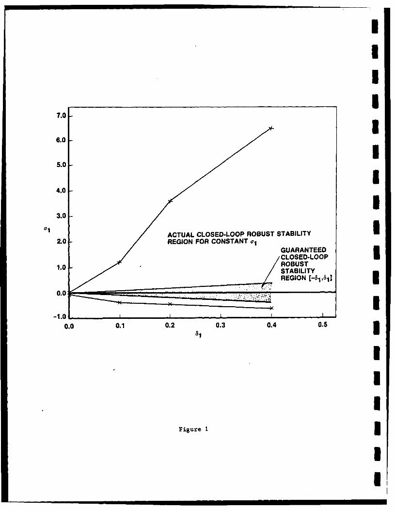
7.0

6.0

5.0

4.0

3.0

01ACTUAL CLOSED-LOOP ROBUST STABILITYI

2.0 REGION FOR CONSTANTGUARANTEEDCLOSED-LOOP

1.0 ROBUSTSTABILITYREGION C-4i'6iI

0.0

0001020.3 0.4 0.53

Figure 1I

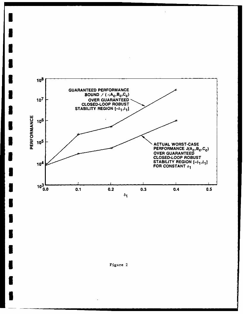
3 108

GUARANTEED PERFORMANCE

107 BOUND/ '(y;AcBcfCc)

OVER GUARANTEED

w

0I Uto ACTUAL WORST-CASEa. PERFORMANCE J(AcBcCc)

OVER GUARANTEEDCLOSED-LOOP ROBUST

10 STABILITY REGION [-61,611FOR CONSTANT

0.0 0.1 0.2 0.3 0.4 0.5

3 Figure 2

II

(81 9 r1 ) Ac B c I

_._-14.91 1.0 1.91 [-

(.2.2) [-17.963 1.0 1 18.9631 [-6.6011 -5.4614]

[133.65 -4.4614J 127.05J

(.4.,) [ 47.813 1.0 48.813 r1-.. 6 -,463 3-1087.3 -6.5463 1073.5 1-376 -756

II

Table 1 I

IIII

N REFERENCES

1. M. G. Safonov and M. Athans, "Gain and Phase Margin for Multiloop LQG Regulators," IEEETrans. Autom. Contr., Vol. AC-22, pp. 173-179, 1977.

2. J. C. Doyle, 'Guaranteed Margins for LQG Regulators," IEEE Trans. Autom. Contr.,Vol. AC-23, pp. 756-757, 1978.

3. J. C. Doyle and G. Stein, "Robustness with Observers," IEEE Trans. Autom. Contr., Vol. AC-3 I24, pp. 607-611, 1979.4. J. C. Doyle and G. Stein, "Multivariable Feedback Design: Concepts for a Classical/Modern

Synthesis," IEEE Trans. Autom. Contr., Vol. AC-26, pp. 4-16, 1981.5. G. Zames, "Feedback and Optimal Sensitivity: Model Reference Transformations,

Multiplicative Seminorms, and Approximate Inverses," IEEE Trans. Autom. Contr., Vol.AC-26, pp. 301-320, 1981.

6. J. C. Doyle, "Analysis of Feedback Systems with Structured Uncertainties," 1EE Proc.,* Vol. 129, pp. 242-250, 1982.

7. M. G. Safonov, "Stability Margins of Diagonally Perturbed Multivariable Feedback Systems,"3 EE Proc., Vol. 129, pp. 251-256, 1982.8. G. Zanes and B. A. Francis, "Feedback, Minimax Sensitivity, and Optimal Robustness," IEEE

Trans. Autom. Contr., Vol. AC-28, pp. 585-601, 1983.3 9. G. Stein and M. Athans, "The LQG/LTR Procedure for Multivariable Feedback ControlDesign," IEEE Trans. Arutom. Contr., Vol. AC-32, pp. 105-114, 1987.

10. B. A. Francis, A Course in Ho, Control Theory, Springer-Verlag, New York, NY, 1987.11. E. Soroka and U. Shaked, "On the Robustness of LQ Regulators," IEEE Trans. Autom.

Contr., Vol. AC-29, pp. 664-665, 1984.12. U. Shaked and E. Soroka, "On the Stability Robustness of the Continuous-Time LQG Optimal

Control," IEEE Trans. Autom. Contr., Vol. AC-30, pp. 1039-1043, 1985.13. M. Tahk and J. L. Speyer, "Modeling of Parameter Variations and Asymptotic LQG Synthesis,"

Proc. 24th IEEE Conf. Dec. Contr., pp. 1459-1465, Athens, Greece, December 1986.14. S. S. L. Chang and T. K. C. Peng, "Adaptive Guaranteed Cost Control of Systems with

Uncertain Parameters," IEEE Trans. Autom. Contr., Vol. AC-17, pp. 474-483, 1972.15. R. V. Patel, M. Toda and B. Sridhar, "Robustness of Linear Quadratic State Feedback Designs

in the Presence of System Uncertainty," IEEE Trans. Autom. Contr., Vol. AC-22, pp. 945-949, 1977.3 16. G. Leitmann, "Guaranteed Asymptotic Stability for a Class of Uncertain Linear DynamicalSystems," J. Optim. Thy. Appl., Vol. 27, pp. 99-106, 1979.

17. A. Vinkler and L. J. Wood, "Multistep Guaranteed Cost Control of Linear Systems with3 Uncertain Parameters," J. Guid. Contr., Vol. 2, pp. 449-:456, 1979.18. M. Eslami and D. L. Russell, "On Stability with Large Parameter Variations: Stemming from

the Direct Method of Lyapunov," IEEE Trans. Autom. Contr., Vol. AC-25, pp. 1231-1234,1980.

19. M. Corless and G. Leitmann, "Continuous State Feedback Guaranteeing Uniform UltimateBoundedness for Uncertain Dynamical Systems," IEEE Trans. Autom. Contr., Vol. AC-26,1139-1144, 1981.

20. J. S. Thorp and B. R. Barmish, "On Guaranteed Stability of Uncertain Linear Systems via3 Linear Control," J. Optim. Thy. App!., Vol. 35, pp. 559-579, 1981.

I

21. B. R. Barmish, M. Corless and G. Leitmann, "A New Class of Stabilizing Controllers for UUncertain Dynamical Systems," SIAM J. Contr. Optim., Vol. 21, pp. 246-255, 1983.

22. B. R. Barmish, I. R. Petersen and A. Feuer, "Linear Ultimate Boundedness Control of IUncertain Dynamic Systems," Automatica, Vol. 19, pp. 523-532, 1983.

23. B. R. Barmish, "Necessary and Sufficient Conditions for Quadratic Stabilizability of anUncertain Linear System," J. Optim. Thy. Appl., Vol. 46, pp. 399-408, 1985.

24. R. K. Yedavalli, S. S. Banda and D. B. Ridgely, "Time-Domain Stability Robustness Measuresfor Linear Regulators," J. Guid. Contr. Dyn., Vol. 8, pp. 520-524, 1985. 3

25. A. R. Galimidi and B. R. Barmish, "The Constrained Lyapunov Problem and its Applicationto Robust Output Feedback Stabilization," IEEE Trans. Autom. Contr., Vol. AC-31, pp. 410-419, 1986. 3

26. I. R. Petersen and C. V. Hollot, "A Riccati Equation Approach to the Stabilization of UncertainSystems," Automatica, Vol. 22, pp. 397-411, 1986.

27. G. Leitmann, E. P. Ryan and A. Steinberg, "Feedback Control of Uncertain Systems:Robustness with Respect to Neglected Actuator and Sensor Dynamics," Int. J. Contr., Vol.43, pp. 1243-1256, 1986.

28. 0. I. Kosmidou and P. Bertrand, "Robust-Controller Design for Systems with Large ParameterVariations," Int. J. Contr., Vol. 45, pp. 927-938, 1987.

29. D. C. Hyland and D. S. Bernstein, "The Optimal Projection Equations for Fixed-OrderDynamic Compensation," IEEE Trans. Autom. Contr., Vol. AC-29, pp. 1034-1037, 1984.

30. D. S. Bernstein and D. C. Hyland, "The Optimal Projection Equations for Finite-DimensionalFixed-Order Dynamic Compensation of Infinite-Dimensional Systems," SIAM J. Contr.Optim., Vol. 23, pp. 122-151, 1986.

31. D. S. Bernstein, "The Optimal Projection Equations for Static and Dynamic Output Feedback:The Singular Case," IEEE Trans. Autom. Contr., Vol. AC-32, pp. 1139-1143, 1987.

32. D. S. Bernstein and W. M. Haddad, "LQG Control With An H. Performance Bound,"submitted to IEEE Trans. Autom. Contr..

33. D. S. Bernstein, "Robust Static and Dynamic Output Feedback Stabilization: Deterministic Uand Stochastic Perspectives," IEEE Trans. Autom. Contr., Vol. AC-32, pp. 1076-1084, 1987.

34. Y. A. Phillis, "Controller Design of Systems with Multiplicative Noise," IEEE Trans. A utom.Contr., Vol. AC-30, pp. 1017-1019, 1985.

35. D. S. Bernstein and S. W. Greeley, "Robust Controller Synthesis Using the Maximum EntropyDesign Equations," IEEE Trans. Autom. Contr., Vol. AC-31, pp. 362-364, 1986. 3

36. D. S. Bernstein and D. C. Hyland, "The Optimal Projection Equations for Reduced-OrderModelling, Estimation and Control of Linear Systems& with Multiplicative White Noise,"J. Optim. Thy. Appi., Vol. 58, 1988, to appear.

37. S. Richter, "A Homotopy Algorithm for Solving the Optimal Projection Equations for Fixed-Order Dynamic Compensation: Existence, Convergence and GloLal Optimality," Proc. Amer.Contr. Conf., pp. 1527-1531, Minneapolis, MN, June 1987. 3

38. S. W. Greeley and D. C. Hyland, "Reduced-Order Compensation: LQG Reduction VersusOptimal Projection Using a Homotopic Continuation Method," Proc. IEEE Conf Dec.Contr., pp. 742-747, Los Angeles, CA, December 1987.i

39. A. Gruzen, "Robust Reduced Order Control of Flexible Structures," C. S. Draper LaboratoryReport #CSDL-T-900, April 1986.

!U

40. A. Gruzen and W. E. Vander Velde, "Robust Reduced-Order Control of Flexible StructuresUsing the Optimal Projection/Maximum Entropy Design Methodology," AIAA Guid. Nav.3 Contr. Conf., Williamsburg, VA, August 1978.

41. J. W. Brewer, "Kronecker Products and Matrix Calculus in System Theory,* IEEE Trans.Circ. Sys., Vol. CAS-25, pp. 772-781, 1978.

42. J. K. Hale, Ordinary Differential Equations, Wiley, New York, 1969.43. J. Warga, Optimal Control of Differential and Functional Equations, Academic Press,

New York, 1972.44. L. Arnold, Stochastic Differential Equations: Theory and Applications, Wiley, New York, 1974.45. C. R. Rao and S. K. Mitra, Generalized Inverse of Matrices and It. Applications, John Wiley

* and Sons, New York, 1971.46. A. Packard and J. C. Doyle, "Robust Control with an H2 Performance Objective,' Proc. Amer.

Contr. Conf., pp. 2141-2145, Minneapolis, MN, June 1987.

II'II'I

IIII

"I IaII

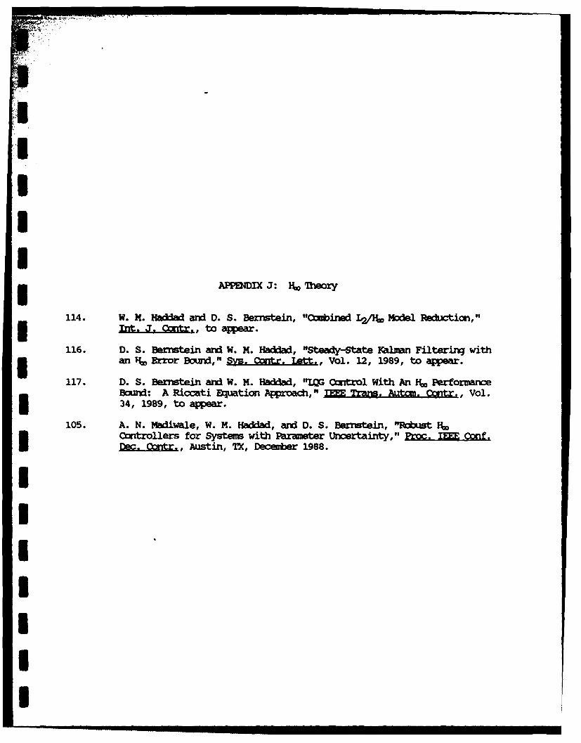
I!

APPEOIIX J: 16~ fwory

114. W. M. Ha and D. S. Bernstein, "bined L2/16 Model R Ction,"Int. J. gg=t. , to aer

116. D. S. Bernstein and W. M. Hadad, "Ste&4-Stte aman Filtering with3 an % Error Bound," Svs. Ccrtr. Lett., Vol. 12, 1989, to apear.

117. D. S. Bernstein and W. M. Haddad, "tILG ontrol With An Nl PerforwanceBound: A Riccati Equation Approach," I Trans. Autc . Contr., Vol.34, 1989, to appear.

105. A. N. Madiwale, W. M. Haddad, and D. S. Bernstein, 'oust fICntrollers for Systems with Parameter Uncertainty," Proc. 1= Qnf.Dc t, Austin, TX, December 1988.

iIIIIII

I.

February 1988Revised April 1988

Combined L 2/H.. Model ReductionII,

by

I,Wassim M. Haddad Dennis S. Bernstein

I Dept. of Mechanical Engineering Harris CorporationFlorida Institute of Technology Government Aerospace Systems Division

Melbourne, FL 32901 MS 22/4848Melbourne, FL 32902

II

I Abstract

i A model-reduction problem is considered which involves both L2 (quadratic) and Ho (worst-case frequency-domain) aspects. Specifically, the goal of the problem is to minimize an L2 model-reduction criterion subject to a prespecifie-, H,, constraint on the model-reduction error. Theprincipal result is a sufficient condition for characterizing reduced-order models with boundedL 2 and H, approximation error. The sufficient condition involves a system of modified Riccatiequations coupled by an oblique projection, i.e., idempotent matrix. When the H(, constraint isabsent, the sufficient condition specializes to the L 2 model-reduction result given in Hyland andBernstein, 1985.

Supported in part by the Air Force Office of Scientific Research under contract F49620-86-C-0002

I

1. Introduction

One of the most fundamental problems in dynamic systems theory is to approximate a high- 3order, complex system with a low-order, relatively simpler model. The resulting reduced-order

model can then be used to facilitate the analysis of complex systems as well as the design and 3implementation of feedback controllers and electronic filters. The model-reduction problem thus

reflects the fundamental engineering desire for simplicity of implementation and parsimony of hard- 3ware.

In view of the practical motivations for the model-reduction problem, it is not surprising that Isignificant effort has been devoted to this problem in recent years. Indeed, there now exists a well-

developed theoretical foundation for model reduction under a variety of approximation criteria. IExpanding on the original work of Adarjan, Arov and Krein, 1971, progress was achieved in Kung

and Lin, 1981, Lin and Kung, 1982, Glover, 1984, Latham and Anderson, 1985, Hung and Glover, 31986, Anderson, 1986, Ball and Ran, 1987, and Parker and Anderson, 1987, for the Hankel-norm

approximation criterion. Many of the cited works also present bounds for the closely related H,,3

approximation error, although the optimal H. model-reduction problem remains open. Alterna-

tively, early progress on the model-reduction problem with a quadratic (L 2 ) criterion was achieved 3in Wilson, 1970, and further explored in Hyland and Bernstein, 1985.

Although the Hankel norm, H, and L2 model-reduction criteria represent distinct approxi- Imation objectives, there exist significant connections. For example, it was shown in Wilson, 1985,

that for systems which are either single input or single output, the input and output space topolo- Igies can be redefined so that the induced norm of the Hankel operator coincides with the L2

system norm. In addition, the optimization technique utilized in Wilson, 1970, was reapplied to 3the Hilbert-Schmidt Hankel operator topology in Wilson, 1988. In recent work, Wilson, 1988a,

has shown that for single-input or single-output systems the quadratic model-reduction criterion is 3actually an induced norm of the convolution operator itself.

In the present paper we attempt a further unification of the L2 and Ho model-reduction m

objectives. Specifically, we consider an L2 model-reduction problem with a constraint on the Ho

approximation error. The underlying idea involves the suitable application of a frequency-domain iinequality due to Willems, 1971, which has recently been applied to H, control-design problems

in Petersen, 1987, Khargonekar, Petersen and Zhou, 1987, and Bernstein and Haddad, 1988. The 3principle result of the present paper is a sufficient condition which characterizes reduced-order U

. ... ," " n -m."m i i f i mm 'mmlI .. .. i1

Um

models satisfying an optimized .L 2 bound as well as a prespecified H.. bound. The sufficient

condition is a direct generalization of the optimal projection approach developed in Hyland and

Bernstein, 1985, for the unconstrained L2 problem. While the L2-optimal reduced-order model

was characterized in Hyland and Bernstein, 1985, by means of a coupled system of two modified

Lyapunov equations, the H,,-constrained solution in the present paper involves a coupled system

consisting of four modified Riccati equations. As in Hyland and Bernstein, 1985, the coupling isIdue to the presence of an oblique projection (idempotent matrix) which determines the constrained

reduced-order model. When the H,, constraint is sufficiently relaxed, we show that the conditions

given herein specialize directly to those given in Hyland and Bernstein, 1985. Although our result

gives sufficient conditions for H,,o approximation, we also state hypotheses under which these

3 conditions are also necessary.

Although numerical algorithms were developed in Hyland and Bernstein, 1985, for the "pure"

L 2 problem, computational methods for the H,,-constrained problem are beyond the scope of the

present paper. In view of the additional complexity engendered by the H. constraint, more sophis-

ticated algorithms appear necessary. Hence computational methods will focus on the homotopic

continuation algorithm developed in Richter, 1987, for reduced-order dynamic compensation.

3 Notation and Definitions

m., iRr X, r , iE real numbers, r x a real matrices, IR" xl, expected value3 (r,( )T,Orx.,Or r x r identity matrix, transpose, r x a zero matrix, Orxr

( )* complex conjugate transpose

3 tr trace

O'm&x(Z) largest singular value of matrix Z

I m.(Z) largest eigenvalue of matrix Z with real spectrum

lIZ1I'i [tr ZZ*]i (Frobenius matrix norm)I I~~t~l fl0 I~h~t)ll~dtJJ

II1H()112 [-L 00= JIH(jJJ2)II I

IIH(s)1 00 SupweIR 07- [H(jw)]

3 r, IN r , IPr r x r symmetric, nonnegative-definite, positive-definite matrices

Z, 5Z 2 , Z,< Z 2 Z 2 -_Z E IN,Z 2 _Z 1 p' Z1 , Z 2 ESr

U n, m, n.., q, p; i positive integers; n + n,,

z, 1y Yin, f,, f,, , , 1, i -dimensional vectors

2

Y'= Y- Yin) z,,

A,B,C n x n,n x m,t x n matrices

D, E m x p, q x matrices

A.,B.,C,. nm X n,,,n,, X m,t X n.. matrices 1[A I1 rBl ( _

BD= [ D] EC=[EC -ECI,.]

R ETE, model-reduction error-weighting matrix in IPt

W() p-dimensional standard white noise process

intensity of Dw(.),V = DDT E IP"[CRC CTRC,] [BVBT BVB.]

I-y positive constant

2. Statement of the Problem

In this section we introduce the model-reduction problem with constrained H.. norm of the

model-reduction error. Specifically, we constrain the transfer function of the reduced-order model

to lie within a specified Hoo radius of the original system. In this paper we assume that the

full-order model is asymptotically stable, i.e., the matrix A is asymptotically stable.

H,,-Constrained L 2 Model-Reduction Problem. Given the nth-order controllable andobservable model1

o(t) = Az(t) + BDw(t), (2.1)

y(t) = CX(t), (2.2) 3where t E [0, oo), determine an nith-order model I

i,,(t) = A,,,(t) + B,,,Dw(t), (2.3) Iy!m(t) = C. X,(t), (2.4)

which satisfies the following criteria: 1(i) Am is asymptotically stable;

3

I

3 (ii) the transfer function of the reduced-order model is within a radius-t H..3 neighborhood of the full-order model, i.e.,

IIH(s) - H.(s)Iloo _<, (2.5)

where

H(s) -A EC(sI. - A)-BD, H, () A- EC.(sI... - A,)-B,D, (2.6)

and -y > 0 is a given constant; and

(iii) the L 2 model-reduction criterion

J(A,'B,, C) A li IE f{[Y(t)- Y.(t)] T R[y(t) -m(t)]} (2.7)

3 is minimized.

Note that the full- and reduced-order systems (2.1)-(2.4) can be written as a single augmentedU systemSi(t) = ,ik(t) + bw(t), t E [0, oo), (2.8)

so that the q x p transfer function from w(t) to Ej(t) = ti(t) is

fr(a) = k(Si, - j)-b (2.9)

I and (2.7) can be written as

3 J(A.,E., C) = liM I{ [Eg(t)]T [Eg(t)] } =,lini [, T (t)jAt)]. (2.10)

Before continuing it is useful to note that if A,. is asymptotically stable then the L 2 model-reduction criterion (2.7) is given by

J(A.m,Bm , C) = tr jA, (2.11)

3where the steady-state covariance

A lim IE gqtiT~t)] (2.12)

4I -o

satisfies the augmented Lyapunov equation

O = AC+ 1A T +VC. (2.13)

Using (2.11) and (2.13) it can be shown that the L 2 criterion (2.7) is an approximation measure3

involving the full- and reduced-order impulse responses with respect to an L2norm.

Proposition 2.1. The L2 model-reduction criterion (2.11) can be written as3

B(Am, ,rnC.) = 'EeBD - E -eAtBm,,D! dt, (2. 14a)

or, equivalently,f00

J(Am, Bm, Cm) = f Hj)-Hmj)jdJ (2.14b)

Proof. It need only be noted that (2.11) is equivalent to

trjf0 eAtf'eArtdtR = trj0 .Ate~bbTe.irT tTdt

= trjfo( eAtb)(te,4'b)Tdt

f 100 112 IIdt

which is equivalent to (2. 14a). Finally, (2.146) follows from Plancherel 's Theorem. 0

The key step in enforcing (2.5) is to replace the algebraic Lyapunov equation (2.13) by an

algebraic Riccati equation. Justification for this technique is provided by the following result.

Leinna 2.1. Let (Am, Bm, C,) be given and assume there exists Q E IRfl"f satisfying

Q E INR (2.15)3

and O AQ +Q.IT + _ 2 !Q +V (2.16)

Then

(idf2QrQ + fji) is stabilizable (2.17)

if and only if

Furthermore, in this case, Am is asymptotically stable. (2.18)

jjH(s) - Hm(a)IIo . '7 (2.19)

5

Q < Q, (2.20)

* and

J(A, .B.C.) 5 J(AmB,,.,C,. Q), (2.21)

where

J(m,B.,,Cm, Q) - tr QR. (2.22)

Proof. Using the assumed existence of a nonnegative-definite solution to (2.16) and the sta-

bilizability condition (2.17), it follows from the dual of Lemma 12.2 of Wonham, 1979, that A is

asymptotically stable. Since A is block diagonal, Am is also asymptotically stable. Conversely,since A is assumed to be asymptotically stable, (2.18) implies (2.17). The proof of (2.19) follows

from a standard manipulation of (2.16); for details see Lemma 1 of Willems, 1971. To prove (2.20)

subtract (2.13) from (2.16) to obtain

0 = A(Q -) + (Q _ )AT + T-Q Q, (2.23)

which, since A is asymptotically stable, is equivalent to

-Q - o = 00 eAt1f 2Q eATtdt > 0. (2.24)

Finally, (2.21) follows immediately from (2.20). 0

Lemma 2.1 shows that the H.. constraint is automatically enforced when a nonnegative-definite

solution to (2.16) is known to exist. Furthermore, the solution Q provides an upper bound for the

actual state covariance Q along with a bound on the L2 model-reduction criterion. Next, we present

a partial converse of Lemma 2.1 which guarantees the existence of a nonnegative-definite solution

to (2.16) when (2.19) is satisfied.

3 Lemma 2.2. Let (Am, Bi, C,) be given, suppose A is asymptotically stable, and assume the

Ho, approximation constraint (2.19) is satisfied. Then there exists a unique nonnegative-definite

solution Q satisfying (2.16). Furthermore, (A+,y-2 QA, ") is stabilizable if and only if +-y-Q2

is asymptotically stable.

3 Proof. The result is an immediate consequence of Theorems 3 and 2, pp. 150 and 167 of

Brockett, 1970, and the dual of Lemma 12.2 of Wonham, 1979. 0

I Finally, we show that the quadratic term -1-2!2Q Q in (2.16) also constrains the Hankel norm

of the approximation error Ej when Q is positive definite. To show this let P E IN be the

6

I

II

observability Gramian for the augmented system (A, D; E) which satisfies

0 = A T P + PjA + R. (2.25) 1

Furthermore, note that Q satisfying (2.13) is the dual controllability Grarnian.

Proposition 2.2. Let (A,, B,,C,,) be given and assume there exists Q E IP satisfying

(2.16) and (2.17) or, equivalently, (2.18). Then 1

AL (PQ) . (2.26)

Proof. Since Q is invertible, (2.16) implies

o = 92ATQ-1 +,y 2 Q- + Q-VQ- + A. (2.27)

Next, subtract (2.25) from (2.27) to obtain

0 = AT(Q1 - _f7) + (2Q-1 - fA + 72 Q Q 1 , (2.28)I

which, since A is asymptotically stable, is equivalent to 37 - P = jo e Ajt [,2QlVQI1e~tdt > 0. (2.29)1

Thus, (2.29) implies P < 1Q- 1 or, equivalently, QiPQ i < -. Hence, A~max(PQ) -y ". Finally,

(2.26) follows immediately from (2.20). 0 13. The Auxiliary Minimization Problem and Necessary Conditions for Optimality I

As discussed in the previous section, the replacement of (2.13) by (2.16) enforces the H.l

approximation constraint between the full- and reduced-order systems and results in an upper

bound for the L 2 model-reduction criterion. That is, if (2.16) is solvable then the reduced-order

model (Am, B,,,,Cm,.) satisfies the H. approximation constraint (2.5) while the actual L2 model-

reduction criterion is guaranteed to be no worse than the bound given by J(A,, r,, Cm., Q).

Hence, J(Am, B,, C, Q) can be interpreted as an auziliary cost which leads to the following

mathematical programming problem.

Auxiliary Minimization Problem. Determine (Am, B,,Cm, Q) which minimizes

J(A,B.,,C.., Q) subject to (2.15) and (2.16). 37 1

I It follows from Lemma 2.1 that the satisfaction of (2.15)-(2.17) leads to 1) A, stable; 2) a

bound on the H, distance between the full-order and reduced-order systems; and 3) an upper

bound for the L 2 model-reduction criterion. Hence it remains to determine (Am,, Bin, C.) which

minimizes J(A,B,,C,, Q) and thus provides an optimized bound for the actual L 2 criterion

J(A., B,,C.,). Rigorous derivation of the necessary conditions for the Auxiliary Minimization

Problem requires additional technical assumptions. Specifically, we restrict (A,,, B,C,, Q) toIthe open set

S _ {(A,,B,,C,,,Q) :Q eIP, A+Q,-Q is asymptotically stable,

and (Am, B.,C,) is controllable and observable}. (3.1)

I HRemark 3.1. The set S constitutes sufficient conditions under which the Lagrange multiplier

technique is applicable to the Auxiliary Minimization Problem. Specifically, the requirement that

Q be positive definite replaces (2.15) by an open set constraint, the stability of A + .- Q serves

as a normality condition, and (Am, B.,C.) minimal is a nondegeneracy condition.

The following Lemma is needed for the statement of the main result.

Lemma 3.1. Let QEi C IN" and suppose rank nP =. T" en there exist nn x n G,Ir

and n, n,, invertible M, unique except for a change of basis in IR", such that

I P= GT rm , (3.2)

3 rGT = in-. (3.3)

Furthermore, the n x n matrices

r A GTI, (3.4)

Tj A. -,r (3.5)

are idempotent and have rank n.m and n - n, respectively. If, in addition,

rank Q = rank P = n., (3.6)

3 thenthenQ - fr (3.7),(3.8)

Finally, if P E IN" then the inverse

S (In + _f- 2 P)-' (3.9)

8

-

I

exists. I

Proof. Conditions (3.2)-(3.8) are a direct consequence of Theorem 6.2.5 of Rao and Mitra,

1971. To prove that the inverse in (3.9) exists, note that since the eigenvalues of P coincide withthe eigenvalues of the nonnegative-definite matrix PS Piit follows that P has nonnegative

eigenvalues. Thus, the eigenvalues of I + '- 2 Qp are all greater than one so that the above inverse

exists. 0

Finally, for convenience define

Theorem 3.1. If (A,,Bm,C,, Q) E S solves the Auxiliary Minimization Problem then

there exist Q, P, Q, P E IN' such that 3A, = r(A - -- 4QQPS)GT, (3.10)

A. = rB, (3.11)

C. = C(I. + _-2QPS)GT, (3.12)

Q- I, (3.13)

and such that Q, P, Q, P satisfy I

0 = AQ + QAT + "Y-2Q.Q + r.LETI, (3.14) I0 -- ATP + PA - "_-4 STpQEQPS + rI(. + -QPS)T(I. + ,- 2QPS)r±, (3.15)

0 = (A - -y-4Q QPS) + (A - f- 4 Q2QPS)T + ,-4 STPQ2QPS + E - r.Erf, (3.16) I0 = (A + - Q 2)Tp + P(A + 1 -2Q2) + (I" + -QpS)T2(I. + 7-2 QPS)

- rf(I,, + .1- 2QpS)T2(I. + - 2 QPS)rj., (3.17) IrankQ= rank P = rank =. . (3.18) 3

Furthermore, the auxiliary cost is given by

J(A., B.,C.,Q) = tr 2(Q + 7- 4QPS STPQ). (3.19)

Conversely, if there exist Q, P,, E IN" satisfying (3.14)-(3.18), then (A,, Bm,C,, Q) given by I(3.10)-(3.13) satisfy (2.15) and (2.16) with the auxiliary cost (2.22) given by (3.19).

9

I

I

Proof. See Appendix A. [

Remark 3.1. Theorem 3.1 presents necessary conditions for the Auxiliary Minimization

Problem which explicitly synthesize extremal reduced-order models (A., B,,C.). As a check

of these conditions, consider the extreme case , = n. Then G = F- and thus, without lo

of generality, G = r = r = I, and r- = 0. Furthermore, (3.14) implies that Q = 0 and (3.15)

implies that P = 0. Hence the Hoe-constrained full-order model is given (as expected) by (A, B,C)

regardless of y. Furthermore, note that Q given by (3.13) becomes

9 Q=[ 4 (3.20)

so that the quadratic term '- 2 QAQ in (2.16) vanishes. Thus (2.16) reduces to (2.13) so that

Q coincides with the controllability Gramian Q. If, alternatively, the reduced-order constraint

is retained but the transfer function approximation constraint (2.5) is sufficiently relaxed, i.e.,

7 -* oo, then S = I. so that the reduced-order model (3.10)-(3.12) is given by (A., B,Cm) =

I (FAGTr,FB,CGT). In this case (3.14) and (3.15) are superfluous and (3.16) and (3.17) reduce to

the optimal projection equations obtained by Hyland and Bernstein, 1985, for the unconstrained

3 L2 problem.

4. Sufficient Conditions for Combined L 2 /l. Approximation

In this section we combine Lemma 2.1 with the converse of Theorem 3.1 to obtain our main

result guaranteeing constrained H. approximation along with an optimized L3 model-reduction

bound.

I Theorem 4.1. Suppose there exist Q,P,Q,P E IN" satisfying (3.14)-(3.18) and let

(A., B.,Cm,Q) be given by (3.10)-(3.13). Then (.i,[71-2QAQ + vji) is stabilizable if and only

if Am is asymptotically stable. In this case, the reduced-order transfer function H,.(s) satisfies the

H., approximation constraintI3I q(s) - ff.(,)II.@< (4.1)

and the L 2 approximation bound

U fI H(s) - H.(s)I, < [ tr 4(q+ -qpS( STPQ)*. (4.2)

I Proof. The converse portion of Theorem 3.1 implies that Q given by (3.13) satisfies (2.15) and

(2.16) with auxiliary cost given by (3.19). It now follows from Lemma 2.1 that the stabiizability

10

I

condition (2.17) is equivalent to the asymptotic stability of A., the H. approximation condition U(2.19) holds, and the L3 model-reduction criterion satisfies the bound (2.21) which is equivalent to 3(4.2). 0

In applying Theorem 4.1 the principal issue concerns conditions on the problem data under

which the coupled Riccati equations (3.14)-(3.17) poesm nonnegative-definite solutions. Clearly,

for -y sufficiently large, (3.14)-(3.17) approximate the "pure" L. solution obtained in Hyland and

Bernstein, 1985. In practice, we would numerically solve (3.14)-(3.17) for successively smaller values

of -y until solutions are no longer obtainable. The important case of interest, however, involves small

-1 so that accurate H.. approximation is enforced Thus, if (4.1) can be satisfied for a given -1 > 0

by a class of reduced-order models, it is of interest to know whether one such reduced-order model I

can be obtained by solving (3.14)-(3.17). Lemma 2.2 guarantees that (2.16) posess" a solution

for any model satisfying (4.1). Thus our sufficient conditions will also be necessary so long as the 3Auxiliary Minimization Problem possesses at least one extremal over S. When this is the case we

have the following immediate result. 3Proposition 4.1. Let -y" denote the infimum of (IH(s) - H.(s) J), over all asymptotically

stable reduced-order models and suppose that the Auxiliary Minimization Problem has a solution 3for all -1 > -y'. Then for all -y> -1* there exist Q,P,4,fA E IN' satisfying (3.14)-{3.17).

Remark 4.1. As in Hyland and Bernstein, 1985, it can be expected that (3.14)-(3.17) possess Imultiple solutions. Theorem 4.1 guarantees, however, that the bounds (4.1) and (4.2) are enforced

for all such extremals obtained by solving (3.14)-(3.17). I

IIIIII

11

I

I

U Apprndix A: Proof of Theorem 3.1

To optimie (2.22) over the open et S subject to the constraint (2.16), form the Lagrangamn

.(A..,B..,C, ,,P,A) - tr(AQA + [AQ + QAT+'F-Q{Q +,P}, (A.l)

where the Lagrange multipliers A ?! 0 and P E I are not both zero. We thus obtain

A= (,+ _,QA)TP + P(A + - ' Q) + Ak. (A.2)

Setting f- = 0 yields

0 = (A + -Y-1 QR)p + P(A + -Y1QA) + AR. (A.3)

Since A+-t is amsumed to be stable, A = 0 implies P = 0. Hence, it can be assumed without

Ices of generality that A = I. Furthermore, P is nonnegative definite.

Now partition A x Ai Q,P, into n x n,n x v., and . x n,. subblocks as

[i Q.,] ... [,,QS Q.Q2 ' A= e, '

3and for notational convenience define

~ Z1 Z12 1

i Zi = ,Q + p 2 Q, Z13 p1Q12 + p12Q,,q,= pr2Q, + pQr , Z2 p ,Q,

I ~ ~ ~ ~ ~ 3 Ths wit AQ1 + 1 h tainiycndtos r ivnb

I1aQ = (A+ .QOA)Tp + P(A+,_Q)+ f=0, (A.4)

,= Z = 0, (A.5)

1 = PiB2 BV + P2 B,V = 0, (A.6)aB,.

I a_m 2RCm Q + 21 2 QRCZ1 2Qi, - 2RCQ,2 - -RCZTQ1 2

- -RCQZ, 12 - -RCZTQ 2 =0. (A.7)

12

I

Expanding (2.16) and (A.4) yields

0 = AQI + QIAT + - 2(QtCT - Qt1 CI)R(QiCT - Q12CI)r + BVB r , (A.8) IAQ12 + Q1A r + -2QICrRCQ - -Q 2 CjRCQj 2 _•_Y- QICTR

+ ,Y-2 qC~rRC.q,, (A.9)

o = Qq2 + QA+ A" - ,(QCr - QC~r)R(QrCr - QCr)r + B TVBr , (A.1)

o - 1 A!P + PIA + -I- 2CTRCZT - -- ISCTRC".Z + t-'z, CrRC

- - Z12C,,RC + CTRC, (Al)

S- ATP12 + P 2A. + -7- 2CrRCZ7 - "-2 ZC T RC. + - 2 Zl3C RC. - CrRC., (A.12)

o = AT P2 + P2A. - f-yCT.RCZ - -- Z,1 CrRC., + C.RC.,. (A.13) 3Now define the n x n matrices

= IQ,, TQ, I ,p_ PT,,Qr± Qt - Q12 q , 1 , P , P 12

and the n., x n, n", x n,, and n. x n matrices

G!L -- IQrT, M 2 r- QP ,, -- PITP2

The existence of Q - and P'-I follows from the fact that (A., B.,Cm.,) is minimal. See Bernstein I

and Haddad, 1988, and Hyland and Bernstein, 1985, for details. Note that r = GTr. Clearly,

Q,P, Q, and P are symmetric and nonnegative definite.

Next note that with the above definitions, (A.5) implies (3.3) and that (3.2) holds. Hence

r = GT[ ' is idempotent, i.e., r2 = r. Sylvester's inequality yields (3.18). Note also that (3.7) and

(3.8) hold.

The components of Q and P can be written in terms of Q, P,Q,P,G, and r as

Q,=Q+q, P,=P+P, (A.14)

Q,2 = rrl' P1 2 = -PG , (A.15) IQ2 = ri T, P2 = UPGT . (A.16) I

13 I

I

Next note that by using (A.14)-(A.16), (A.7) becomes

I C,,.9 = C[I. + -I-(Q + i)PGT,

U where

i .. + -FrQPGT.

To prove that S is invertible use (3.7) and (3.4) and note that

I.- + -- 2 N PG r = i.. + Y-'7 rTPGT

= 1,. + Y-'(r r7)(GPGT).

Since V rT and GPGT are nonnegative definite, their product has nonnegative eigenvalues. Thus

each eigenvalue of In_ +-y-f. 2 (IPGT is real and is greater than unity. Hence is invertible. Now

note that by using (3.3) and (3.4) it can be shown that

I GT§-lr = Sr.

The expressions (3.11), (3.12) and (3.13) follow from (A.6), (A.7), (3.9) and the definition of Q3 by using the above identities. Next, computing either r(A.9)-(A.10) or G(A.12)+(A.13) yields

(3.10). Substituting this expression for Am into (A.8)-(A.13) it follows that (A.10) = I'(A.9) and

(A.13) = G(A.12). Thus, (A.10) and (A.13) are superfluous and can be omitted. Next, using

(A.8)+GTP(A.9)G - (A.9)G - [(A.9)G]T and GrI(A.9)G - (A.9)G- [(A.9)G]T yields (3.14)

and (3.16). Using (A.11) + rTG(A.12) r- (A.12)Ir - [(A.12) r]T and VrG(A.12)f - (A.12)F -

[(A.12)r]T yields (3.15) and (3.17).

i Finally, to prove the converse we use (3.10)-(3.18) to obtain (2.16) and (A.4)-(A.7). Let

Am, B.,C.,G,r, r,Q,P,(,], Q be as in the statement of Theorem 3.1 and define Q,,Q 1 2,Q2,

P,,P 2 ,P by (A.14)-(A.16). Using (3.3), (3.11) and (3.12) it is easy to verify (A.6) and (A.7).

Finally, substitute the definitions of Q,P,.,f,G,], and r into (3.14)-(3.17) along with (3.3),

i (3.4), (3.7) and (3.8) to obtain (2.16) and (A.4). Finally, note that

which shows that > 0. 0

14

I

I

References 3Adarnjan, M., Arov, D. Z., and Krein, M. G., 1971, Math. USSR Sbornik, 15, 31; 1978, 3

Amer. Math. Soc. Trans., 111, 133.Anderson, B. D. 0., 1986, Sys. Contr. Lett., 7, 247.

Ball, J. A., and Ran, C. M., 1987, SIAM J. Contr. Optim., 25, 362.Bernstein, D. S., and Haddad, W. M., 1988, "LQG Control with an H, Performance Bound:

A Riccati Equation Approach,* IEEE Trans. Autom. Contr., submitted. 3Brockett, R. W., 1970, Finite Dimensional Linear Systems, (Wiley).

Glover, K., 1984, Int. J. Contr., 39, 1115.

Hung, Y. S., and Glover, K., 1986, Sys. Contr. Left., 7, 165.Hyland, D. C., and Bernstein, D. S., 1985, IEEE Trans. Autom. Contr., 30, 1201.Khargonekar, P. P., Petersen, 1. R., and Zhou, K., 1987, "Robust Stabilization of Uncertain

Systems and HI Optimal Control," preprint.Kung, S.-Y., and Lin, D. W., 1981, IEEE Trans. Autom. Contr., 26, 832.Latham, G. A., and Anderson, B. D. 0., 1985, Sys. Contr. Left., 5, 229. ILin, D. W. and Kung, S.-Y., 1982, Cir. Sys. Sig. Proc., 1, 407.

Parker, P. J., and Anderson, B. D. 0., 1987, Int. J. Contr., 46, 1783.Petersen, I. R., 1987, IEEE Trans. Autom. Contr., 32, 427.Rao, C. R., and Mitra, S. K., 1971, Generalized Inverse of Matrices and Its Applications,

(John Wiley and Sons). IRichter, S., 1987, Proc. Amer. Contr. Conf., June 1987, Minneapolis, MN, 1527.Willems, J. C., 1971, IEEE Trans. Autom. Contr., 16, 621.

Wilson, D. A., 1970, Proc. IEE, 117, 1161. IWilson, D. A., 1985, Int. J. Contr., 42, 65.Wilson, D. A., 1988, "System Order Reduction Using the Hilbert-Schmidt Norm of the

Hankel Operator," preprint. IWilson, D. A., 1988a, "Convolution and Hankel Operator Norms for Linear Systems,"

IEEE Trans. Autom. Contr., to appear. IWonham, W. M., 1979, Linear Multivariable Control: A Geometric Approach, (Springer-Verlag)

I!!III

I

I March 1988Revised June 1988I

ISteady-State Kalman Filtering with an

H,. Error Bound

I

I by

UDennis S. Bernstein Wassim M. HaddadHarris Corporation Department of Mechanical and

Government Aerospace Systems Division. Aerospace EngineeringMS 22/4848 Florida Institute of Technology3 Melbourne, FL 32902 Melbourne, FL 32901

i

I AbstractAn estimator design problem is considered which involves both L 2 (least squares) and Ho.

(worst-case frequency-domain) aspects. Specifically, the goal of the problem is to minimize an L2

state-estimation error criterion subject to a prespecified Ho constraint on the state-estimation er-ror. The H,. estimation-error constraint is embedded within the optimization process by replacingthe covariance Lyapunov equation by a Riccati equation whose solution leads to an upper boundon the L2 state-estimation error. The principal result is a sufficient condition for characterizingfixed-order (i.e., full- and reduced-order) estimators with bounded L 2 and H,, estimation error.The sufficient condition involves a system of modified Riccati equations coupled by an obliqueprojection, i.e., idempotent matrix. When the H,, constraint is absent, the sufficient conditionspecializes to the L 2 state-estimation result given in (2].

I Keywords: Kalman filter, Ho, norm, reduced-order state estimation, optimal projection equa-tions, Hankel norm.I

Supported in part by the Air Force Office of Scientific Research under contract F49620-86-C-0002.

I

I

1. Introduction 1One of the fundamental problems in dynamic systems theory is the observation of state vari- I

ables. Although an extensive theoretical foundation has been developed for the quadratic (least

squares) error criterion, state estimation with a worst-case frequency-domain design objective has 3apparently not been considered. In the present paper we thus extend the least squares formulation

to include a frequency-domain bound on the state-estimation error. The underlying idea involves

the application of state-space techniques which have recently been developed for H, control design

in [1,4--61. The results of the present paper are thus complementary to the results obtained in [11.

The principal result of the present paper is a sufficient condition which yields full- and reduced-

order estimators satisfying an optimized L 2 error bound as well as a prespecified Ho. error bound.

In the full-order case, the H,,-constrained estimator involves a modified Riccati equation which

specializes to the standard steady-state Kalman filter when the H,, constraint is absent. In the Ireduced-order case the Hoo-constrained result leads to a direct generalization of the optimal pro-

jection approach developed in [2] for the unconstrained L2 state-estimation problem. While the

L 2-optimal reduced-order state estimator was characterized in [2] by means of a coupled system of

one modified Riccati equation and two modified Lyapunov equations, the H -constrained solution 3involves a coupled system consisting of three modified Riccati equations and one modified Lya-

punov equation. As in [2], the coupling is due to the presence of an oblique projection (idempotent Imatrix) with additional coupling now arising from the Ho. constraint. When the H,. constraint is

sufficiently relaxed, these conditions again specialize directly to those given in [2]. 3We note that the development in the present paper is limited to the case in which the plant

is asymptotically stable. These results can also be extended to the unstable plant case, although Iwith additional complexity. This case will thus be treated in a future paper.

The contents of the paper are as follows. After collecting notation in Section 2, the statement

of the Ho.-Constrained State-Estimation Problem is given in Section 3. The principal result of this

section (Lemma 3.1) shows that if the algebraic Lyapunov equation for the covariance is replaced

by a modified Riccati equation possessing a nonnegative-definite solution, then the H0 estimation- Ierror constraint is enforced and the L 2 state-estimation error criterion is bounded above by an

auxiliary cost function. The problem of determining a reduced-order estimator which minimizes Ithis upper bound subject to the Riccati equation constraint is considered in Section 4 as the

Auxiliary Minimization Problem. Necessary conditions for the Auxiliary Minimization Problem I1!

, i i l I I II

U (Theorem 4.1) are given in the form of a coupled system of modified algebraic Riccati equations.

To develop connections with standard Kalman filter theory the full-order estimator result is also

given. In Section 5 the necessary conditions of Theorem 4.1 are combined with Lemma 3.1 to yield

sufficient conditions for bounded H.. and L2 estimation error. Although our result gives sufficient

conditions for H.. estimation error, we also state hypotheses under which these conditions are also

necessary (Proposition 5.1).

2. Notation and Definitions

m, iR r Xe, i r , iE real numbers, r x s real matrices, IRr"x , expected value

Ir, ( )T,Orx*,O r x r identity matrix, transpose, r x s zero matrix, Orxr

tr trace

3 Omax(Z) largest singular value of matrix Z

Amax(Z) largest eigenvalue of matrix Z with real spectrum

I IIZIIF [tr ZZ]JI (Frobenius matrix norm)

IIH(s)Iloo supwrlm 0rM&X[H(jw)j

3 5 r, INr, ]pr r x r symmetric, nonnegative-definite, positive-definite matrices

ZI < Z2 , Z 1 < Z2 Z 2 - Z IN , Z 2 -Z IP, Z1 , Z2 S

n, 1, n., p, q, r; fi positive integers; n + n.; n, < n

Pz, Y ye, 0, , n, t, q, n., fi-dimensional vectors

A,C n x n, x n matrices

D1 ,D 2 , E n x p,t x p,r x q matrices

5 L q x n matrix

A,, B,, C, n, x , n, x £,q x n, matrices

* A [A~ 0Oz [EB.C A.

5 [EL [-C

R ETE, estimation error weighting in IPq

I W(.) p-dimensional standard white noise process

V1,V2 intensity of Diw(.),D 2w(.); V = DDTE IN",V 2 - D2 DTE IPt

1 2

I

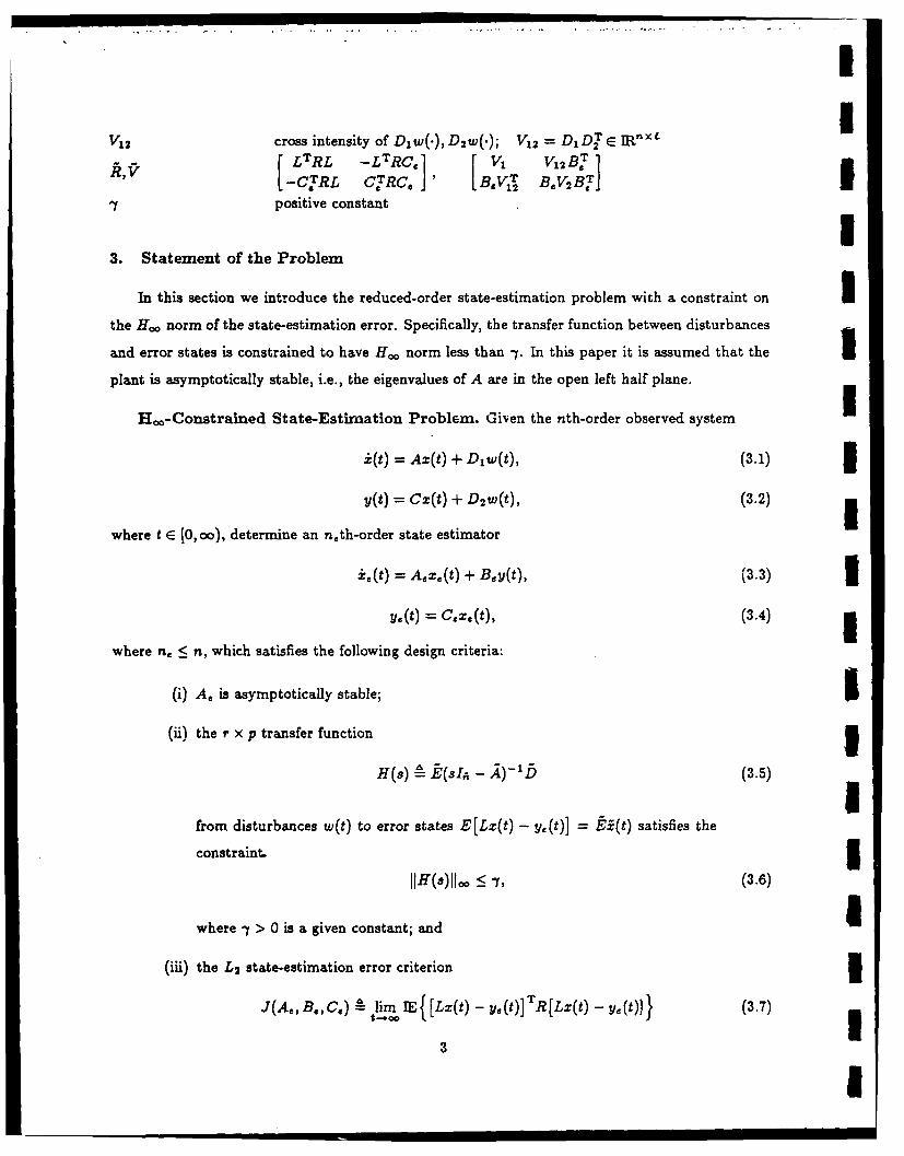
II I

VI2 cross intensity of Diw(.),D 2 w(-); V12 = DIDT E IR " f-

1?, r L TRL ._L TRC. [1 1 2BR,V I-CT'RL CTRC, 'V BB V2

7y positive constant I3. Statement of the Problem

In this section we introduce the reduced-order state-estimation problem with a constraint on Uthe Ho norm of the state-estimation error. Specifically, the transfer function between disturbances

and error states is constrained to have H.o norm less than y. In this paper it is assumed that the I

plant is asymptotically stable, i.e., the eigenvalues of A are in the open left half plane.

Ho-Constrained State-Estimation Problem. Given the nth-order observed system

i(t) = Az(t) + D w(t), (3.1)

y(t) = Cx(t) + D2 0~), (3.2)

where t E [0, oo), determine an nth-order state estimator

i.(t) = Aex(t) + Bey(t), (3.3)

Y(t = C.z.(t), (3.4)

where n, < n, which satisfies the following design criteria:

(i) A. is asymptotically stable; S(ii) the r x p transfer function 1

H~s) A- tC..,x, - j)-Ib (3.5)

from disturbances w(t) to error states E[Lx(t) - y,(t)] = E(t) satisfies the

constraint. 5ll/-r(s)l 0 _< 7, (3.6)

where -y > 0 is a given constant; and U(iii) the L 2 state-estimation error criterion 5

J(AeB.,C.) A lim IE { [Lx(t) .i(t)] T R[Lx(t) - .i(t)I (3.7)

3

U is minimized.

I It is useful to note that the augmented system (3.1)-(3.4) can be written as

3 i(t) = Ai(t) + bw(t), t E [0,o), (3.8)

3 and that (3.7) is equivalent to

J(A., B., C.) = i IE I [&j(t)1T IIji(t)] } i IE~[i T(t)A~gt)]. (3.9)

Furthermore, if A, is asymptotically stable for a given estimator (A,, B,, C,) then the L 2 state-

3 estimation error criterion is given by

J(A., B,,C.) = tr QR, (3.10)

where the steady-state covariance defined by

0lim lE[i(t)iTct)] (3.11)

I satisfies the h x f. Lyapunov equation

0 AQ + A T + f/. (3.12)

Using (3.10) and (3.12) we now show that the criterion (3.7) is an error measure involving the

impulse response of (3.8) with respect to an L2 norm.

3 Proposition 3.1. If A. is asymptotically stable then the L2 state-estimation error criterion

(3.7) can be written as

J(A., B,, C.) = f IIeAtbldt. (3.13)

3 Proof. It need only be noted that (3.10) is equivalent to

tr o 0e0CVeA T tdt I = tr jo 0(teAtb)(keAtb)Tdt,

which is equivalent to (3.13). [1

i The key step in enforcing (3.6) is to replace the algebraic Lyapunov equation (3.12) by an

algebraic Riccati equation. Justification for this technique is provided by the following result.

4

I

II

Lemma 3.1. Let (A., B, C) be given and assume there exists Q E R' R4 satisfying UQ E IN" (3.14) 1

andI

o = AQ +Q!AT+ -I2 Q +f. (3.15)Then I

(A, [_,- QQ + ]) is stabilizable (3.16) Iif and only if

A, is asymptotically stable. (3.17) 1Furthermore, in this case

Q _ Q, (3.19) Iand

J(A.,B.,C.) '(A.,B.,Cc, Q), (3.20) 1where

J(Ae,B.,Cc,Q) A tr QRk. (3.21) 1Proof. Using the assumed existence a nonnegative-definite solution to (3.15) and the stabi- l

lizability condition (3.16), it follows from the dual of Lemma 12.2 of [9] that A is asymptotically

stable. Since A is lower block triangular, A asymptotically stable implies A, is asymptotically sta- 3ble. Conversely, since A is assumed to be asymptotically stable, (3.17) implies A is asymptotically

stable and thus (3.16) holds. The proof of (3.18) follows from a standard manipulation of (3.15); 1for details see Lemma 1 of [8). To prove (3.19) subtract (3.12) from (3.15) to obtain

0 A(Q - Q) + (Q - Q)AT + - 2 QR , (3.22) Iwhich, since A is asymptotically stable, is equivalent to I

- 0= e1t[.-2Q TQ]e dt > 0. (3.23)

Finally, (3.20) follows immediately from (3.19). 0

5 I

ILemma 3.1 shows that the Ho constraint is automatically enforced when a nonnegative-definite

I solution to (3.15) can be shown to exist. Furthermore, the solution Q provides an upper bound for

the steady-state covariance q along with a bound on the L2 state-estimation error criterion. Next,

we present a partial converse of Lemma 3.1 which guarantees the existence of a nonnegative-definite

solution to (3.15) when (3.18) is satisfied.

3 Lemma 3.2. Let (A, B,,C,) be given, suppose A. is asymptotically stable, and assume the

H,, state-estimation error constraint (3.18) is satisfied. Then there exists a unique nonnegative-

definite solution Q satisfying (3.15). Furthermore, (A + -y- 2 QR, D) is stabilizable if and only if

A + -- 2QR? is asymptotically stable.

3Proof. The result is an immediate consequence of Theorems 3 and 2 of [3], pp. 150 and 167,

along with the dual of Lemma 12.2 of [9]. 0

IFinally, we show that the quadratic term -- 2 .Q!RQ in (3.15) also constrains the Hanke! norm

of the estimation error E[Lz(t) - y.(t)] when Q is positive definite. To show this let P E IN be

the observability Gramian for the augmented system (A, E t) which satisfies

0 = ATP + 1 A+j. (3.24)

1Proposition 3.2. Let (A., B.,C,) be given and assume there exists Q E IP satisfying (3.15)

and (3.16) or, equivalently, (3.17). Then

<AMaX(PQ (3.25)

Proof. Since Q is invertible, (3.15) implies

5 0 = ,.2iTQ-1 + t 2 .Q 1-A + Y2 .Q 1-Q 1 + . (3.26)

3Next, subtract (3.24) from (3.26) to obtain

50o = jT(,2Q-1 - .5) + (,Q- 1 _ !')A + 7 2 Q-rQ-', (3.27)

g which, since A is asymptotically stable, is equivalent to

2Q-1 = eAT t[ 72Q Q-1]eCAtdt> 0. (3.28)

61I

I_ _ I

Thus (3.28) implies < .y2Q- or, equivalently, Q2PQ2 < -y2 1-. Hence,

4. The Auxiliary Minimization Problem and Necessary Conditions for Optimality

As discussed in the previous section, the replacement of (3.12) by (3.15) enforces the H, istate-estimation error constraint and results in an upper bound for the L 2 state-estimation error

criterion. That is, given an estimator (A,, B,,C.) satisfying the H.0 estimation constraint, the 5actual L2 state-estimation error criterion is guaranteed to be no worse than the bound given by

J(A.,B.,C., Q) if (3.15) is solvable. Hence, J(A., B,,C., Q) can be interpreted as an auziliary

cost which leads to the following optimization problem.

Auxiliary Minimization Problem. Determine (A,, B,, C,, Q) which minimizes J(A,, B., IC,, 2) subject to (3.14) and (3.15). 1

It follows from Lemma 3.1 that the satisfaction of (3.14)-(3.16) leads to 1) A. stable; 2) Hoo

estimation error bound -y; and 3) an upper bound (3.21) for the L 2 state-estimation error criterion. 3Hence it remains to determine (A,, B,,C.) which minimizes J(A., B.,C., Q) and thus provides

an optimized bound for the actual L2 criterion J(A,, B,, C.). Rigorous derivation of the neces-

sary conditions for the Auxiliary Minimization Problem requires additional technical assumptions.

Specifically, we restrict (A., B.,C,, Q) to the open set 3S A {(A.,B.,C.,Q) : Q E IP;, A + Q-22R is asymptotically stable,

and (A., B,, C.) is controllable and observable}. I

Remark 4.1. The set S constitutes sufficient conditions under which the Lagrange multiplier

technique is applicable to the Auxiliary Minimization Problem. Specifically, the requirement that

Q be positive definite replaces (3.14) by an open set constraint, the stability of A + f- 2 Qk serves

as a normality condition, and (A,, B.,C.) minimal is a nondegeneracy condition.

The following Lemma is needed for the statement of the main result.

Lemma 4.1. Let ,P E IN" and suppose rank e]P = n.. Then there exist n, x n G, r and

n. x n, invertible M, unique except for a change of basis in IR' " , such that 5= GTMr, (4.1)

7 a

I FGT= In.. (4.2)

3 Furthermore, the n x n matrices

r A GTr, (4.3)

r = In --r, (4.4)

3 are idempotent and have rank n, and n - n, respectively. If, in addition,

5 rark c rankP = n., (4.5)

then r , = /r. (4.6),(4.7)

3 Finally, if P E INn then the inverse

3 A i (+. - p)- (4.8)

exists.

Proof. Conditions (4.1)-(4.7) are a direct consequence of Theorem 6.2.5 of [71. To prove that

the inverse in (4.8) exists, note that since the eigenvalues of P coincide with the eigenvalues of

the nonnegative-definite matrix PI Pf, it follows that QP has nonnegative eigenvalues. Thus,the eigenvalues of I + -2P are all greater than one so that the above inverse exists. 0

Finally, for arbitrary Q E IR xn n define the notation

I q QCT+ V1 2 , EALTRL. (4.9)

Theorem 4.1. If (A,, B., C., Q) E $ solves the Auxiliary Minimization Problem then there

3 exist Q, P,QP E IN" such that

A, = r(A - Q.V71 C -1 -C4 QQPS)GT , (4.10)

B. = rQ . vj-1, (4.1)

3 C, = L(I. + -r-QPS)GT, (4.12)

Q= r+¢ r rT (4.13)

8I

and such that Q, P, 1J, P satisfy

-Q T + V, + - 2QEQ - Q IVi Q + r.LQV 2 Q.r., (4.14)1

o -- ATP+ PA - Lr-STpQ,,QPS + rI(I. + + _QPS)r., (4.15) 30 = (A - .- 4QQPS)Q + Q(A - ,-4QEQPS)T + _- 4 QSTPQEQPSQ

+QV 21Q- rQVqi .TrI, (4.16)

0 = (A - Q.Vi-'C + -QE)TP + P(A - Q.Vi-'C +,"- 2 QZ)+ (I, + _f- 2QpS)TZ(I. + '- 2QPS) -rT(I + - 2QpS)T,(I. + _- 2 QPS)r±, (4.17) 1

rank ¢ = rank P = rank 15 = n.. (4.18) 1Furthermore, the auxiliary cost is given by

J(A., B.,C,,Q) = tr LTRL(Q + "7-4QPSQSTpQ). (4.19)

Conversely, if there exist Q, P, Q, P E INn satisfying (4.14)-(4.18), then (A., B.,Ce, Q) given by £(4.10)-(4.13) satisfies (3.14) and (3.15) with the auxiliary cost (3.21) given by (4.19).

Proof. See Appendix A. 0

Remark 4.2. Theorem 4.1 presents necessary conditions for the Auxiliary Minimization Prob- 3lem which explicitly synthesize extremal full- and reduced-order estimators (A., B,, C,). If the H,0

estimation constraint is sufficiently relaxed, i.e., -1 --+ oo, then S = I,,. In this case equations (4.16) 3and (4.17) become decoupled from (4.15) and thus (4.15) becomes superfluous. Furthermore, (4.14),

(4.16) and (4.17) specialize to the optimal projection equations obtained in [2]. 3As discussed in [2], in the full-order (Kalman Filter) case n, = n, G = F- 1 and thus G = r

r = I,, and rT. = 0 without loss of generality. To develop further connections with the standard IKalman filter theory assume = (4.20)

In this case (4.15) implies that P = 0 so that the gain expressions (4.10)-(4.12) become I

A. = A - QCTVi-lC, (4.21)

B. = QcTvi- 1, (4.22) 1C. = L,(4.23)

9 a

while equations.(4.14)-(4.16) and auxiliary cost (4.19) specialize to

1 0= AQ + QAT+ V, + - 2 QLTRLQ - QCTV 2-1CQ, (4.24)

3 J(A., B.,CQ) = tr LTRLQ. (4.25)

Remark 4.3. Note that the necessary conditions for the full-order problem involve one modi-

fied Riccati equation. This equation is similar to the observer Riccati equation with the additional

quadratic term - 2QLTRLQ. Finally, note that when the H,, estimation constraint is sufficiently

relaxed, i.e., -y - o, (4.24) reduces to the standard observer Riccati equation of steady-state

3 Kalman filter theory.

3 5. Sufficient Conditions for Combined L 2 /H,, Estimation

In this section we combine Lemma 3.1 with the converse of Theorem 4.1 to obtain our main

result guaranteeing constrained H.. state-estimation error and an optimized L 2 state-estimation

error bound.

I Theorem 5.1. Suppose there exist Q, P,Q,] E IN' satisfying (4.14)-(4.18) and let (A., B.,

C., Q) be given by (4.10)-(4.13). Then (A, [- 2QRQ + V ] ) is stabilizable if and only if A, isU asymptotically stable. In this case, the transfer function H(s) defined by (3.5) satisfies the Ho,

state-estimation error constraint

g and the L 2 state-estimation error criterion (3.7) satisfies the bound

J(A,,B,,C,) < tr LTRL(Q + -- 4QPS STpQ). (5.2)

Proof. The converse portion of Theorem 4.1 implies that Q given by (4.13) satisfies (3.14)3 and (3.15). It now follows from Lemma 3.1 that the stabilizability condition (3.16) is equivalent

to the asymptotic stability of A., the H.. state-estimation error constraint (3.18) holds, and the5 L2 state-estimation error criterion (3.7) satisfies the bound (3.20) which, by (4.19), is equivalent

to (5.2). 3

I In applying Theorem 5.1 the principal issue concerns conditions on the problem data under

which the coupled Riccati equations (4.14)-(4.17) Rossess nonnegative-definite solutions. Clearly,

10

I

for -y sufficiently large, (4.14)-(4.17) approximate the pure least squares problem considered in

[2]. The important case of interest, however, involves small -y so that significant H". estimation Iis enforced. Thus, if (5.1) can be satisfied for a given -y > 0, it is of interest to know whether

one such fixed-order estimator can be obtained by solving (4.14)-(4.17). Lemma 3.2 guarantees Ithat (3.15) possesses a solution for any fixed-order estimator satisfying (5.1). Thus our sufficient

conditions will also be irecessary so long as the Auxiliary Minimization Problem possesses at least

one extremal over S. When this is the case we have the following result.

Proposition 5.1. Let -y" denote the infimum of IIH(s)IoI over all asymptotically stable fixed- Iorder estimators and suppose that the Auxiliary Minimization Problem has an extremal for all

-y > -". Then for all -y> -y* there exist Q,P,Ci,P E IN' satisfying (4.14)-(4.17). IAppendix A: Proof of Theorem 4.1

To optimize (3.21) over the open set S subject to the constraint (3.15), form the Lagrangian

C(A.,B.,C.,.Q, PA) - tr {AQR+ [AQ + QAT+ - 2 QRQ + V]P}, (A.) Iwhere the Lagrange multipliers A > 0 and P E IR4x" are not both zero. We thus obtain 3

aCI L --- 2!2 1 )T p + p ( A + _- 2 . 1 ) + A . (A .2 )

Setting = 0 yields I

0= (+. -2 Q')Tp + P(A + _Y-2 2! ) + AA. (A.3) ISince A+ -,-2 Q? is assumed to be stable, A = 0 implies P = 0. Hence, it can be assumed without 3loss of generality that A = 1. Furthermore, P is nonnegative definite.

Now partition fi x h Q,P into n x n,n x n,, and n, x n, subblocks as 5.Q Q1 Q2] P1 P12Sp 2 ]' IQT12 Q2j PIT P2J

and for notational convenience define

PQ ZI 12 1LZ= 1 Z2 J'

where +4, PIQ1 + P12q12 Z2,Q2+P22

Z A p q1 + pZQT 2, z pTQ12 + P2Q2.

11

a

Thus, with A = I the stationarity conditions are given by

I a + _21)Tp+p(,+ _-!1)+R=0, (A.4)

I a _

8A. = Z2 = 0, (A.5)

aC = Z 2 CT+ PI2 VI2 + P2 B.V2 = 0, (A.6)aB a

= 2RC.Q 2 + 2- 2RCZQ 12 - 2RLQ12 -1-2RLZTQ1

3-1 JRLQ1Z12 - _- 2 RLZTIQ 2 =0. (A.7)

I Expanding (3.15) and (A.4) yields

0 = AQ, + QiAT + V + _Y-2(QLT- Q22Cl)R(QLT Q1 2C)T, (A.8)

3 0 = AQ 12 + Q 2 AT+ QiCTBT+V12 BT +.f- 2 QLTRLQ12 - - 2 Q1 2 CTRLQ12

- -Q,LTRC.Q 2 + -2 Q12 CTRC.Q 2 , (A.9)IIoA.Q2 + Q2AT + B.CQ12 + QT CTB4T+ B.V2 BT3 + "- 2 (QTLT - Q2C,)R(QT LT - Q2C,)T, (A.10)

0= ATPI, + P1 A + CTB P + P12BC + -T- 2LTRLZT + 1 2 ZILTRL

5 -2 L-LTRC.ZiT _ _-2Z,2 CRL + LTRL, (A.11)

0 = ATP,12 + P12 A, + CTBTP2 + f- 2LTRLZT -y-2 ZILTRC.

+1-2Z 12 CTRC. - LTRC., (A.12)

0 = ATP2 + P2A, - 7- 2 C.TRLZ T - -Z 2 ,LTRC. + CTRC.. (A.13)

Now define the n x n matrices

3 q A- Q - Q1 2Q2 1q 2, P P P- P12P - p T ,

= q 12 -q T , pA P12 p-

12 - I I T 2

-and the n. x n,n, x n,, and n, x n matrices

GA Q-IQ, 12=t P , C - -P .

I

The existence of Q- 1 and P-1 follows from the fact that (A., B6, C) is minimal. See [1,2] for

details. Note that r = GTr. Clearly, Q, P, Q, and P are symmetric and nonnegative definite. INext note that with the above definitions, (A.5) implies (4.2) and that (4.1) holds. Hence

r = GTr is idempotent, i.e., r2 = r. Sylvester's inequality yields (4.18). Note also that (4.6) and 5(4.7) hold.

The components of Q and P can be written in terms of Q,P, ,?,G, and F as IQ =Q+Q, P, = P+ P, (A.14) IQ 1 2 =Qr T , P12 =PfGT, (A.15)

Q2 = FQ T , P2 = GPG T. (A.16) 5

Next note that by using (A.14)-(A.16), (A.7) becomes

C.S = L[I. + _- 2 (Q + )P]GT,

where II" . + _Y-2 qPGT .

To prove that § is invertible use (4.6) and (4.3) and note that

I.. + 7-2FQPGT = I.. + -1-2p rTpGT I

= 1'. + -- 2 (rvrT)(GPGT).

Since FN1 T and GPGT are nonnegative definite, their product has nonnegative eigenvalues. Thus Ieach eigenvalue of I,,. + - 2 QPGT is real and is greater than unity. Hence S is invertible. Now 1note that by using (4.2) and (4.3) it can be shown that

GTs-2r = Sr. 5The expressions (4.11), (4.12) and (4.13) follow from (A.6), (A.7), (4.8) and the definition of Q

by using the above identities. Next, computing either F(A.9) - (A.10) or G(A.12) + (A.13) yields

(4.10). Substituting this expression for A, into (A.8) - (A.13) it follows that (A.10) = F(A.9)

and (A.13) = G(A.12). Thus, (A.10) and (A.13) are superfluous and can be omitted. Next, using

(A.8) + GTV(A.9)G - (A.9)G - [(A.9)GJT and GTF(A.9)G - (A.9)G - [(A.9)G]T yields (4.14) and

(4.16). Using (A.I1)+TG(A.12)r- (A.12)r-[(A.12)r]T and FTG(A.12)r-(A.12)r-[(A.12)r]T

yields (4.15) and (4.17). 13

I• . . , , ,.,i...... .. i...... .. . i ...

IFinally, to prove the converse we use (4.10)-(4.18) to obtain (3.15) and (A.4) - (A.7). Let

A,,Be,C,,G,J,r,QP,Q,P, Q be as in the statement of Theorem 4.1 and define Q 1 ,Q 12 ,Q 2 ,P 1 ,

P 12 ,P 2 by (A.14)-(A.16). Using (4.4), (4.11) and (4.12) it is easy to verify (A.6) and (A.7). Finally,

subsitute the definitions of Q, P, Q, P, G, r and r into (4.14)-(4.17) along with (4.2), (4.3), (4.6)

Iand (4.7) to obtain (3.15) and (A.4). Finally, note that

*nX 0" = [Q + I~ - I, r,

g which shows that Q >0. 0

I3References

[1] D.S. Bernstein and W.M. Haddad, "LQG Control with an Ho Performance Bound: A RiccatiEquation Approach," Proc. Amer. Contr. Conf., pp. 796-802, Atlanta, GA, June 1988.

[2] D.S. Bernstein and D.C. Hyland, "The Optimal Projection Equations for Reduced-Order StateEstimation," IEEE Trans. Autom. Contr., Vol. AC-30, pp. 583-585, 1985.

[3] R.W. Brockett, Finite Dimensional Linear Systems, Wiley, New York, 1970.

(41 J.C. Doyle, K. Glover, P.P. Khargonekar, and B.A. Francis, "State-Space Solutions to StandardH2 and H,, Control Problems," Proc. Amer. Contr. ConI., pp. 1691-1696, Atlanta, GA, June

5 1988.

[5] P.P. Khargonekar, I.R. Petersen and K. Zhou, "Robust Stabilization of Uncertain Systems and

HI Optimal Control," preprint.

[61 I.R. Petersen, "Disturbance Attenuation and H °° Optimization: A Design Method Based onthe Algebraic Riccati Equation," IEEE Trans. Autom. Contr., Vol. AC-32, pp. 427-429, 1987.

[7] C.R. Rao and S.K. Mitra, Generalized Inverse of Matrices and Its Applications, John Wileyand Sons, New York, 1971.

[81 J.C. Willems, "Least Squares Stationary Optimal Control and the Algebraic Riccati Equation,"IEEE Trans. Autom. Contr., Vol. AC-16, pp. 621-634, 1971.

[9] W.M. Wonham, Linear Multivariable Control: A Geometric Approach, Springer-Verlag, NewYork, 1979.

1

I

Submitted to IEEE TACNovember, 1987

Revised April, 1988

U LQG Control with an H. Performance Bound:A Riccati Equation ApproachI

I

by

IDennis S. Bernstein Wassim M. HaddadHarris Corporation Department of

Government Aerospace Systems Division Mechanical and Aerospace EngineeringMS 22/4848 Florida Institute of Technology

Melbourne, FL 32902 Melbourne, FL 32901(305) 729-2140

Abstract

An LQG control-design problem involving a constraint on H,, disturbance attenuation isconsidered. The H., performance constraint is embedded within the optimization process byreplacing the covariance Lyapunov equation by a Riccati equation whose solution leads to an upperbound on L2 performance. In contrast to the pair of separated Riccati equations of standard LQGtheory, the Ho,-constrained gains are given by a coupled system of three nodified Riccati equations.The coupling illustrates the breakdown of the separation principle for the Hoo-constrained problem.Both full- and reduced-order design problems are considered with an Ho, attenuation constraintinvolving both state and control variables. An algorithm is developed for the full-order designproblem and iliustrative numerical results are given.

U Supported in part by the Air Force Office of Scientific Research under contracts F49620-86-C-0002 and F49620-87-C-0108.I

U

1. Introdnction

The fundamental differences between Wiener-Hopf-Kalman (WHK) control design (for exam- Iple, LQG theory [1]) and H,, control theory (2-4] can be traced to the modeling and treatment

of uncertain exogenous disturbances. As explained by Zames in the classic paper [2], LQG design 5is based upon a stochastic noise disturbance model possessing a fixed covariance (power spectral

density), while H, theory is predicated on a deterministic disturbance model consisting of bounded

power (square-integrable) signals. Since LQG design utilizes a quadratic cost criterion, it follows

from Plancherel's theorem that WHK theory strives to minimize the L 2 norm of the closed-loop fre- 3quency response, while H.. theory seeks to minimize the worst-case attenuation. For systems with

poorly modeled disturbances which may possess significant power within arbitrarily small band- 3widths, Ho, is clearly appropriate, while, for systems with well-known disturbance power spectral

densities, WHK design may be less conservative. 5In addition to the fact that H,, design embodies many classical design objectives [5], it also

presents a natural tool for modeling plant uncertainty in terms of normed Ho, plant neighborhoods. IIn contrast, the H 2 topology has been shown in [6] to be too weak for a practical robustness

theory, while the H,, norm is not only suitable for robust stabilization but is also conveniently 3submultiplicative. Within the WHK state space theory, however, the appropriate robustness model

appears not to be a nonparametric normed plant neighborhood as in Ho, theory, but rather a

parametric uncertainty model. The principal technique for capturing the effects of real parameters

within state space models is Lyapunov function theory (see, e.g., [7-16] and the references therein). 3Such structured uncertainties are difficult to capture nonconservatively within Hoo theory except

with specialized refinements ([171). 3In spite of the fundamental differences between WHK design and H. theory, a significant

connection was discovered in [18]. Specifically, Petersen observed that a modified algebraic Riccati £equation developed for parameter-robust full-state-feedback control can also be utilized to yield

controllers satisfying H. disturbance attenuation bounds. This relationship was further explored 3in [19] where it was shown that Petersen's modified Riccati equation effectively yields the Hoo-

optimal full-state-feedback controller. This result is based upon the fact that quadratic stability I(i.e., stability with a quadratic Lyapunov function) of the system

=x=(A +DFE)z, #(F) <1,m

1!

I is 'quivalent to the stability of A and the small gain condition

3 IlE(sl - A) - D [O < 1.

The results of [19] thus solve the Standard Problem considered in [3,4] for the static full-state-

3 feedback case.

The extension of these results to the Standard Problem for dynamic output-feedback compen-

sation, however, was not given in [18,19]. Within the realm of quadratic robust stabilization, the

dynamic output-feedback problem was addressed in [7]. The results of [7] involve a pair of decou-

pled modified Riccati equations along with an auxiliary inequality. Using different techniques, a

moi- complete solution was obtained in [13,14] involving a coupled system of three modified Riccati

equations for full-order dynamic compensation and a coupled system of four modified Riccati and

Lyapunov equations in the fixed-order (i.e., reduced-order) case as in [20]. The results of [13,141

thus raise the following question: What is the relevance of this system of coupled design equations

to the problem of H, disturbance attenuation via fixed-order compensation?

To begin to address this question the goal of the present paper is to d~velop a design methodology

for fixed-order L 2 optimal control which includes as a design constraint a bound on Hoe disturbance

attenuation. There are three principal motivations for developing such a theory. First, the results

of [18,19] present full-state-feedback controllers whose form is directly analogous to the standard

LQR solution. However, no L 2 interpretation was provided in [18,19] to explain this similarity.

The present paper, however, provides an L 2 interpretation within the context of an Hoe design

constraint. A novel feature of this mathematical formulation is the dual interpretation of the

disturbances. That is, within the context of L 2 optimality the disturbances are interpreted as white

noise signals while, simultaneously, for the purpose of H,, attenuation the very same disturbance

signals have the alternative interpretation of deterministic L 2 functions. This dual interpretation is

I unique to the present paper since stochastic modeling does not play a role in [18,19]. We also note

recent results obtained in [21] which essentially show that the H 2 plant topology can be induced

3 by imposing L 2 and Lo topologies on the disturbance and output spaces, respectively. For further

investigation into the relationships between L 2 and Hoe control, see [22].

l The second motivation for our approach is the simultaneous treatment of both L 2 and Hoe

performance criteria which quantitatively demonstrates design tradeoffs. Specifically, in order to

enforce the H, constraint we derive an upper bound for the L 2 criterion. Minimization of this

upper bound shows that the enforcement of an Ho disturbance attenuation constraint leads directly

2

Ui | i m

I

to an increase in the L 2 performance criterion. Although it would be preferable to minimize the

L 2 criterion directly, this problem will be considered in a future paper. 3The third motivation for our approach is to provide a characterization of fixed-order dynamic

output-feedback controllers yielding specified disturbance attenuation. Existing optimal Hoo design 3methods tend to yield relatively high-order controllers. Intuitively, solving the fixed-order design

equations for progressively smaller Hoo disturbance attenuation constraints should, in the limit, 3yield an H,, optimal controller over the class of fixed-order stabilizing controllers. Although our

main result gives sufficient conditions, we also state hypotheses under which these conditions are 5also necessary (Proposition 4.1). It should also be noted that the inherent coupling among the

modified Riccati equations shows that the classical separation principle of LQG theory is not valid 3for the H,.-constrained full- and reduced-order design problems.

Of course, since the present paper addresses the problem of fixed-order dynamic compensation, 3previous full-state feedback results ([18,19]) are not obtainable as a special case. However, applying

the approach of the present paper to the full-state feedback problem yields results which are similar 3to those of [18,19].

Besides establishing connections with robust stabilizability in state space systems, an imme- Udiate benefit of the modified Riccati equation characterization of Hoo-optimal controllers is the

opportunity to develop novel computational algorithms for controller synthesis. To this end a con- Itinuation algorithm has been developed for solving the coupled system of three modified Riccati

equations. In a numerical study (see Section 8) we have demonstrated convergence of the algorithm 3and reasonable computational efficiency. Homotopy methods were suggested for the coupled Ric-

cati equations because of their demonstrated effectiveness in related problems which also involve 3coupled modified Riccati equations [23-25]. Since H. control problems are solvable by estab-

lished numerical methods [4], it should be stressed that the objective of these numerical studies is 3not to make direct comparisons with existing H,, synthesis algorithms, but only to demonstrate

solvability of the coupled modified Riccati equations. 3The contents of the paper are as follows. After presenting notation at the end of this section,

the statement of the Hoo-Constrained LQG Control Problem is given in Section 2. The principal Iresult of this section (Lemma 2.1) shows that if the algebraic Lyapunov equation for the closed-loop

covariance is replaced by a modified Riccati equation possessing a nonnegative-definite solution, 3then the closed-loop system is asymptotically stable, the Ho, disturbance attenuation constraint is

33

. . • i I I II

I satisfied, and the L2 performance is bounded above by an "auxiliary" cost function. The problem

of determining compensator gains which minimize this upper bound subject to the Riccati equation

constraint is considered in Section 3 as the Auxiliary Minimization Problem. Necessary conditions

for the Auxiliary Minimization Problem (Theorem 3.1) are given in the form of a coupled system of

three modified Riccati equations. In Section 4 the necessary conditions of Theorem 3.1 are combined

with Lemma 2.1 to yield sufficient conditions for closed-loop stability, Ho disturbance attenuation,

and bounded L1 performance. In Section 5 we specialize the results of Section 3 to the case in

which the LQG weights are equal to the H,, weights. This serves to equalize the L2 and Ho, design3 aspects and, through a series of transformations, the results of Section 3 are recast in a simpler

form. These results also clarify connections with [261. To achieve further design flexibility, the

reduced-order control-design problem is considered in Section 6. A simplified qualitative analysis

of the full-order design equations is given in Section 7 to highlight important features with regard3 to existence and multiplicity of solutions. Finally, a numerical algorithm is presented in Section 8

along with illustrative numerical results. A series of designs are obtained to illustrate tradeoffs3 between the L 2 and H, aspects and the conservatism of the L, performance bound. Although in

the present paper the numerical results are limited to the case of full-order dynamic compensation,3 reduced-order designs have been obtained in [27] using Theorem 6.1.

Notation. Note: All matrices have real entriesIR, IRrx*, IRr, IE real numbers, r x s real matrices, lR"x", expected value

l,( )T, OX,, 0,. r x r identity matrix, transpose, r x a zero matrix, Ox,

tr, p( ) trace, spectral radiusSr, jNr, IPr r x r symmetric, nonnegative-definite, positive-definite matrices

3 Z,<Z 2, Z,< Z 2 Z2 -ZEINr, Z2 -ZEIPr, Z1, Z2 Sr

n,mt, nc,p,q,q.o; i positive integers; n + n, (n, < n)3 z,, y, zMe, n, m, £, n,, a-dimensional vectors

A, B, C nx n, nxm, txn matrices

3 A., B., C, n, x n,, n, x t, m x n, matrices

A I A BClB0C A.

w(.) p-dimensional standard white noise

D1 , D2 n x p, t x p matrices; DIDT 0

4

V1, V2 DDT, D2D ; V2 E IPLo DiV.D1 Bov 0" J 1

0n*.xn B,,V 2BT I

El, E2 q x n, q x m matrices; ETE2 = 0

t[El E2C.]R 1, R2 ETEI, ETE; R 2 EIP

R[ Onxn - Ion.xn CyR2 C.J

E,, E2 . q. x n, q.. x m matrices; ET E2, = 0 3k. ~ [Eic. E2.C. 10RI., R2. E100TE1.0, E21:E2.

E,. BRjIB T , CTVi-1C I0, Y nonnegative constant, positive constant

2. Statement of the Problem 3In this section we introduce the LQG dynamic output-feedback control problem with con-

strained Ho disturbance attenuation between the plant and sensor disturbances and the state and 5control variables. Without the L2 performance criterion the problem considered here essentially

corresponds to the Standard Problem of [3,4]. For simplicity we restrict our attention to con- 3trollers of order n, = n only, i.e., controllers whose order is equal to the dimension of the plant.

This constraint is removed in Section 6 where controllers of reduced order are considered. Hence, 1

throughout Sections 2-5 the controller dimension n, and closed-loop plant dimension h n + n.

should be interpreted as n and 2n, respectively. Controllers of order greater than n are generally 3of less interest in practice and thus are not considered in this paper.

Hco-Constrained LQG Control Problem. Given the nth-order stabilizable and detectable 1

plant

i(t) = Ax(t) + Bu(t) + Diw(t), (2.1)3

y =t Cz(t) + D 2 W(t), (2.2)

5

.3

U determine an nth-order dynamic compensator

3o(t) = Aczo(t) + Bey(t), (2.3)

g U(t) = ¢.0(t), (2.4)

which satisfies the following design criteria:

3 (i) the closed-loop system (2.1)-(2.4) is asymptotically stable, i.e., A is asymptotically stable;

(ii) the q. x p closed-loop transfer function

H(8) A ](sla -8 )-1 b (2.5)

from w(t) to E 1joz(t) + E 2 oou(t) satisfies the constraint

IIS(s)II, _ 'y, (2.6)

3 where -y > 0 is a given constant; and

(iii) the performance functional

J(AC,BC,C) = ,lim IE [zT(t)Rlz(t) + uT(t)R2u(t)] (2.7)

U is minimized.

3 Note that the closed-loop system (2.1)-(2.4) can be written as

1 (t) = Ai(t) + bw(t) (2.8)

and that (2.7) becomes

1 J(A.,B,C,)= l~nIE[m ( lt))T (.Ct))]- = im IE [ T(t)j(t)]. (2.9)

I Remark 2.1. Since (A, B,C) is assumed to be stabilizable and detectable the set of nth-order

stabilizing compensators is nonempty.

Remark 2.2. It is easy to show that the performance functional (2.7) is equivalent to the

3more familiar expression involving an averaged integral, i.e.,

J(A--B.,C.) Jim I IE f [J(s)Rz(s) + UT(s)R 2u(s)] dot~ co t

0 6

Remark 2.3. For convenience we assume DDT2 - 0, which effectively implies that the plant

disturbance and sensor noise are uncorrelated. 3Remark 2.4. One may wish to consider a general L2 optimization problem of the form

minllT - UQV 112, where Q is a parameterization of stabilizing controllers. In this case, without a 5constraint on the MacMillan degree of Q, it may be possible to satisfy (2.6) with smaller values of

1- 1

Note that the problem statement involves both L2 and H, performance weights. In particular,

the matrices R1 and R2 are the L2 weights for the state and control variables. By introducing L2- l

weighted variables

z(t) = Eiz(t), v(t) = E2 u(t), Ithe cost (2.7) can be written as

J(AC,BC, C) = lim IE [z (t)z(t) + v'(t)v~t)] 1t .-* Oo

For convenience we thus define R, A ETE, and R2 S E2TE 2 which appear in subsequent expres- Isions. Although an L 2 cross-weighting term of the form 2x(t)TR12 u(t) can also be included, we

shall not do so here to facilitate the presentation. 3For the H. performance constraint, the transfer function (2.5) involves weighting matrices El,,,,

and E2,o for the state and control variables. The matrices R 1, A EloE,, and R2.o A E2ooE 2ooare thus the H.. counterparts of the L2 weights R, and R 2. Although we do not require that Ro

and R2. be equal to R, and R2, we shall require in the next section that R 2 _" = 8R2, where the 3nonnegative scalar P is a design variable. Finally, the condition ET. E2 co = 0 precludes an Ho,

cross-weighting term which again facilitates the presentation. UBefore continuing it is useful to note that if A is asymptotically stable for a given compensator

(A,, B,, C,) then the performance (2.7) is given by

J(A., B.,C.) = tr QR, (2.10)

where the steady-state closed-loop state covariance defined by

A l IE[i(t)i T (t)] (2.11)

satisfies the fi x ii algebraic Lyapunov equation 30 = A + IAT + f. (2.12) 1

7

I

U Remark 2.5. Using (2.10) and (2.12) it can oe shown that the L2 cost criterion (2.7) can be

written in terms of the L2 norm of the impulse response of the closed-loop system. Specifically,

writing Q satisfying (2.12) as00 = j P S eAdt,

(2.10) becomes

3 (A.,B.C,.) = jo IIe DIdt,

where II" lji denotes the Frobenius matrix norm.

I The key step in enforcing the disturbance attenuation constraint (2.6) is to replace the alge-

braic Lyapunov equation (2.12) by an algebraic Riccati equation which overbounds the closed-loop

I steady-state covariance. Justification for this technique is provided by the following result.

SLenmma 2.1. Let (A,, B., C.) be given and assume there exists Q E IR A'xt% satisfying

E INA (2.13)

I and0T= A.Q + Q AT + 2Q-A'Q + f. (2.14)

i Then

3 (,?[.f-A 0 o0Q + 1 ) is stabilizable (2.15)

if and only if

3 A is asymptotically stable. (2.16)

In this case,

3 IIH(s)illo -7 "(2.17)

and .(2.18)

Consequently, J(A.,B,C) .. (A,B,C, !), (2.19)

I whereI J(A., B, C, Q) A tr Qk. (2.20)

IProof. Using the assumed existence of a nonnegative-definite solution to (2.14) and the stabi-

lizability condition (2.15), it follows from the dual of Lemma 12.2 of [28] that A is asymptotically

* 8I.. . . . . . . . . . . . -. . * . . . .

Istable. Conversely, if ,I is asymptotically stable then (2.15) holds. The proof of (2.17) follows from

a standard manipulation of (2.14); for details see Lemma I of 1291. To prove (2.18) subtract (2.12)

from (2.14) to obtain

0= A(Q - ) + + 7 -2 (2.21)

which, since A is asymptotically stable, is equivalent to

0- =f eAt[ 2-QROQ)eArt dt >0. (2.22) IFinally, (2.19) follows immediately from (2.18). 0 3

Remark 2.6. Note that (2.15) is actually a closed-loop "disturbability" condition which is

not concerned with control as such. This condition guarantees that the system does not possess Iunstable undisturbed modes. Of course, if V is positive definite or (A, D) is controllable, then

(2.15) is satisfied. 3Lemma 2.1 shows that the H. disturbance attenuation constraint is automatically enforced

when a nonnegative-definite solution to (2.14) is known to exist. Furthermore, the solution Q

provides an upper bound for the actual closed-loop state covariance Q along with a bound on the

L2 performance criterion. Next, we present a partial converse of Lemma 2.1 which guarantees the

existence of a nonnegative-definite solution to (2.14) when (2.17) is satisfied.

Lenma 2.2. Let (A,, B,, C) be given, suppose A is asymptotically stable, and assume the

disturbance attenuation constraint (2.17) is satisfied. Then there exists a unique nonnegative-

definite solution Q satisfying (2.14). Furthermore, (A + 7-Q], V&) is stabilizable if and only Iif A + -y 2QR4A? is asymptotically stable. 3

Proof. The result is an immediate consequence of [301, using Theorems 3 and 2, pp. 150 and

167, along with the dual version of Lemma 12.2 of [28]. 0

Renmark 2.7. To further, clarify the relationships between the L2 and H.. aspects of the

problem, we note that the closed-loop system can be represented by two possibly different transfer Ufunctions. Specifically, with respect to the L 2 cost criterion, the closed-loop transfer function

between disturbances and controlled variables is given by the triple (A, 1), k) while for the H. Iconstraint the closed-loop transfer function (2.5) corresponds to the triple (A, b, k".).

Finally, it can be shown that the closed-loop Riccati equation (2.14) also enforces a constraint !on the norm of the Hankel operator corresponding to the closed-loop system (A, D, k,) when Q

9

is positive definite. Thus, let J5 E IN" denote the solution to

0 = ATP + ASA + A. (2.23)

and note that P and Q (satisfying (2.12)) are the observability and controllability Gramians, respec-

tively, of the system (A, b, E). As shown in [31], the norm of the Hankel operator corresponding

to (A,b, Et.) is given by AM.(PQ).

Proposition 2.1. Suppose there exists Q E IW4 satisfying (2.14) and such that (2.15) or,

equivalently, (2.16) holds. Then

A.(PQ) <'. (2.24)

Proof. Since Q is assumed to be invertible, (2.14) is equivalent to

0 = 7JSTQ - + Q- 1 A+ O-Q -, + A". (2.25)

Subtracting (2.23) from (2.25) shows that -2 Q 1- P_ 0, or, equivalently, 712 > Q*PQ. Thus,

2 \ A 021 0QPQ) = Amx(P6QP2) Amax(PQ),M

which yields (2.24). 0

I3. The Auxiliary Minimization Problem and Necessary Conditions for Optimality

3 As discussed in the previous section, the replacement of (2.12) by (2.14) enforces the H,,

disturbance attenuation constraint and yields an upper bound for the L2 p,rformance criterion.

3 That is, given a compensator (A0 , B,,C 0 ) for which there exists a nonnegative-definite solution

to (2.14), the actual L 2 performance J(A, BO,CC) of the compensator is guaranteed to be no

worse than the bound given by J(A,, Be, C,, Q). Hence, J(A,, Be, Ce, Q) can be interpreted as an

auziliary cost which leads to the following mathematical programming problem.

3 Auxiliary Minimization Problem. Determine (A,, BeC, Q) which minimizes

J(A,, B, C, Q) subject to (2.13) and (2.14).

It follows from Lemma 2.1 that the satisfaction of (2.13) and (2.14) along with the generic condi-

tion (2.15) leads to 1) closed-loop stability; 2) prespecified H,, performance attenuation; and 3) an

3! upper bound for the L2 performance criterion. Hence it remains to determine (A,, Be, C) which

minimizes 7(A., Be,Cc, Q) and thus provides an optimized bound for the actual L2 performance

* 10

I.,.. . . . . . - . . . . . . . .

II

J(AC, B,, C.). Rigorous derivation of the necessary conditions for the Auxiliary Minimization Prob-

lem requires additional technical assumptions. Specifically, we restrict (A,, B,, C,, Q) to the open

setX A {(A.,B.,C.,Q) : Q E IPA, A + (-- 2y-2, is asymptotically stable, (3.1)l

and (AC, B., Cc) is controllable and observable}.

Remark 3.1. The set X constitutes sufficient conditions under which the Lagrange multiplier

technique is applicable to the Auxiliary Minimization Problem. Specifically, the requirement that

Q be positive definite replaces (2.13) by an open set constraint, the stability of A+ ,-y2 Q !,, serves Ias a normality condition, and (A., B¢,Cc) minimal is a nondegeneracy condition. Note that the

stabilizability condition (2.15) and stability condition (2.16) play no role in determining solutions 3of the Auxiliary Minimization Problem.

The following result presents the necessary conditions for optimality in the Auxiliary Minimiza-

tion Problem. The proof of this result is given in Appendix A as a special case of the corresponding

result for reduced-order dynamic compensation considered in Section 6. As mentioned previously,

we assume that RUoo = # 2 R2.Furthermore, for arbitrary Q, P E IN" define

S A (In + s2 -QP-. (3.2)

Since the eigenvalues of iP coincide with the eigenvalues of the nonnegative-definite matrix

Pi Pl, it follows that Q P has nonnegative eigenvalues. Thus, the eigenvalues of I, +82_1-2~p

are all greater than one so that the above inverse exists.

Theorem 3.1. If (A., B,,C,, Q) E X solves the Auxiliary Minimization Problem then there 3exist Q, P,q E IN" such that

A, = A - Q2 - PS + -2QRo,., (3.3) 3Be = QcTv-1, (3.4) 5C. = -Rj'BTPS, (3.5)

A Q Q 1] (3.6)3

and such that Q, P, £ satisfy 30 = AQ + QAT + V, + -- QR,Q - Q;Q, (3.7) U

II

U

0 = (A+ -1-2 [Q + IR.) T + P(A + Y/-2 [Q + (]Rioo) + R1 - STPEPS, (3.8)

5 0= (A - EPS + -- 2 QRI,.) + (A - EPS + y-'QR 1,)T

+ 'f-12 (Ri0 + # 2STPZPS)4 + qZq. (3.9)

m Furthermore, the auxiliary cost is given by

3 J(A.,B.,CC,Q) = tr[(Q+ )Ri +4STPZPS]. (3.10)

Conversely, if there exist Q, P, Q E IN" satisfying (3.7)-(3.9), then (A,, BeC 0 , Q) given by (3.3)-

(3.6) satisfies (2.13) and (2.14) with auxiliary cost (2.20) given by (3.10).

3 Remark 3.2. If Q and Q are nonnegative definite then the fact that (2.13) is satisfied can

easily be seen by writing Q as 0.m Remark 3.3. Setting # = 0 or, equivalently, E2, = 0, specializes Theorem 3.1 to the "cheap"

Ho, control case in which H,, attenuation between disturbances and controls is not constrained.

In this case S = I,, Q is given by (3.6), and

3 A. = A - p + _-2 QRjo, (3.11)

B = qcTvj-, (3.12)

mC = -R 1 'B P, (3.13)

3 where Q satisfies (3.7), and equations (3.8) and (3.9) become

0 = (A + y-' [Q + q]Rj.)Tp + P(A + -- 2 [Q + q]R1 ) + R, - PEP, (3.14)

m 0= (A- EP+ -y 2QR 1 ) +( (A- EP+- 2QR)T + 1-2 (R. o+ Q'DQ. (3.15)

m Finally, the auxiliary cost reduces to

J(A.,B.,C., Q) = tr((Q + 4)R 1 + (PEP]. (3.16)

Numerical solution of equations (3.7), (3.14) and (3.15) is discussed in Section 8.

I Theorem 3.1 presents necessary conditions for the Auxiliary Minimization Problem which ex-

plicitly synthesize extremal controllers (A,, Be, C,). These necessary conditions comprise a system

12

I

1

of three modified algebraic Riccati equations in variables Q, P and Q. The Q and P equations

are similar to the estimator and regulator Riccati equations of LQG theory, while the ( equation 3has no counterpart in the standard theory. Note that the Q equation is decoupled from the P

and Q equations and thus can be solved independently. The P equation, however, depends on

Q. Thus, regulator/estimator separation only holds in one direction which clearly shows that the

certainty equivalence principle is no longer valid for the design problem under consideration. Fur-

thermore, since the P and equations are coupled, they must be solved simultaneously. Finally,

note that if the H,, disturbance attenuation constraint is sufficiently relaxed, i.e., -Y -" oo, then

the P equation becomes decoupled from the C? equation and thus the e equation becomes super-

fluous. Furthermore, the remaining Q and P equations separate and coincide with the standard

LQG result.

4. Sufficient Conditions for Hw Disturbance Attenuation IIn this section we combine Lemma 2.1 with the converse of Theorem 3.1 to obtain our main 3

result guaranteeing closed-loop stability, Ho, disturbance attenuation, and an optimized L 2 per-

formance bound. 3Theorem 4.1. Suppose there exist Q, P,Q E IN' satisfying (3.7)-(3.9). Then, with

(A., B., C., Q) given by (3.3)-(3.6), (A, [-y 2 QR!o2 Q +VI4) is stabilizable if and only if A is asymp-

totically stable. In this case, the closed-loop transfer function H(s) satisfies the H~, attenuation

constraint 3

and the L2 performance criterion (2.7) satisfies the bound 3J(A, BC,C) !5 tr[(Q + )R1 + QSTPLPS]. (4.2)

Proof. The converse portion of Theorem 3.1 implies that Q given by (3.6) satisfies (2.13) and

(2.14) with auxiliary cost given by (3.10). It now follows from Lemma 2.1 that the stabilizability Icondition (2.15) is equivalent to the asymptotic stability of A, the H, disturbance attenuation

constraint (2.17) holds, and the performance bound (2.19), which is equivalent to (4.2), holds. " IRemark 4.1. In applying Theorem 4.1 it is not actually necessary to check (2.15) which

holds generically. Rather, it suffices to check the stability of A directly which is guaranteed to be Iequivalent to (2.15). 1

13

3l. m- l

In applying Theorem 4.1 the principal issue concerns conditions on the problem data under

which the coupled Riccati equations (3.7)-(3.9) possess nonnegative-definite solutions. Clearly,

for -y sufficiently large, (3.7)-(3.9) approximate the standard LQG result so that existence and

uniqueness are assured. The important case of interest, however, involves small -y so that significant

H.. disturbance attenuation is enforced. Thus, if (4.1) can be satisfied for a given -Y > 0, it is of

interest to know whether one such controller can be obtained by solving (3.7)-(3.9). Lemma 2.2

guarantees that (2.14) possesses a solution for any controller satisfying (4.1). Thus our sufficient

condition will also be neceseary so long as the Auxiliary Minimization Problem possesses at least

one extremal over X. When this is the case we have the following immediate result.

Proposition 4.1. Let -" denote the infimum of IIH(s)II . over all stabilizing nth-order dynamic

compensators and suppose that the Auxiliary Minimization Problem has a solution for all -1 > -y.

Then for all -1 > -y* there exist Q,P,Q E IN' satisfying (3.7)-(3.9).

Unlike the standard LQG result involving a pair of separated Riccati equations, the new result

enforcing Ho, disturbance attenuation involves a nonstandard coupled system of three modifed

Riccati equations. The asymmetry of these equations suggests the possibility of a dual result in

which the modifications to the standard P and Q Riccati equations are reversed. Such a dual result

w'ill generally be different from Theorem 4.1 and thus will yield an improved bound for particular

I problems. This point was demonstrated in [16] for the problem of robust performance analysis.

Due to space limitations, however, we give only a brief outline of the dual Ho, results. Note that

3 J(AC, B,CC) given by (2.10) is also given by

J(Ac, Be, C) "= tr ffi, (4.3)

I where P E INA is the unique solution to (2.23). Next, utilizing (4.3) in place of (2.10), the H.

disturbance attenuation constraint (2.6) can now be enforced by replacing (2.23) by the Riccati

I equation

0 = ,jTp + PA + _P-2"pP + A".. (4.4)

Note that (4.4) is merely the dual of (2.14). We also require the condition dual to (2.15) given by

3 ([,Y- 2 PfP + 0A] *,A) is detectable. (4.5)

Once again, the sufficient conditions for H00 disturbance attenuation involve a coupled system of

three modified Riccati equations dual to (3.7)-(3.9). Similar remarks apply to the reduced-order

case given by Theorem 6.1 below.

* 1

I

5. Alternative Forms of the Riccati Equations

The purpose of this section is to draw connections with recent results obtained in (26]. As

shown in Theorem 4.1, the Riccati equations (3.7)-(3.9) provide sufficient conditions for explicitly

synthesizing controllers (A,, B,, C) satisfying an H, performance bound. In this section we

specialize Theorem 3.1 by setting the LQG weights equal to the Ho" weights, i.e., R, = R1.

and 6 = 1. This specialization leads to considerable simplification by equalizing the L2 and H., 3design aspects. In this case it turns out that the Riccati equations (3.7)-(3.9) can be transformed

to simpler forms which are similar to the results given in [26]. To state the results we require 3some additional notation and a lemma concerning transformations of a pair of nonnegative-definite

matrices. 3Lemma 5.1. Let PQ E IN'. Then the following statements hold.

(i) PQ has nonnegative eigenvalues. I(ii) p(PQ) :_ (<)-I-' if and only if PiQPI < (<),-2I Furthermore, if P is positive definite 3

then p(PQ) :_ (<)--2 if and only if Q _< (<)-P-1.

(iii) Define Z A P(4" + -1 -PQ)-'. Then Z is nonnegative definite, IP(-. + -QP) - I = (I. + - 2PQ)-P, (5.1) 3

and p(ZQ) < -y2 or, equivalently, Q1ZQ2 < -1-2I. Furthermore, Z is positive definite

if and only if P is positive definite. In this case,

Z = (p-1 + (5.2) 3(iv) Suppose p(PQ) < -Y-2 and define Y A P(I,. - -y- 2QP)- '. Then Y is nonnegative definite,

P(r. -T_-2qP)-1 = (I. -1-2pQ)- p, (5.3)

and

QP(I, - _t- 2QP)- 1 = (I, - 72-QP)- 1 QP. (5.4) 3Furthermore, P is positive definite if and only if Y is positive definite. In this case, 3

Y = (P- 1 7- 2 Q)-l. (5.5)

15

U

IProof. The results are easily proven and thus the details are omitted. 0

Proposition 5.1. Let R, = Roo fi = 1, suppose there exist Q,Q E IN' and Z E IP"

satisfying

0 -AQ + QA T + V, + V 1 - 2QRQ - Q2Q, (5.6)

0 = (A + ,y-2QRI)TZ + Z(A + _,-2QRI) + R1 - Z.ZZ + -y-2 ZQEQZ, (5.7)

S0 = (A - ,Z + -Y-2QR)Q + ,(A - EZ + _1-2QR1 )T + ,- 2Q(R1 + ZEZ), + QDQ, (5.8)

p(Z4) < _-2, (5.9)

and let (AC, B.,Cc, Q) be given by

A, = A -Q2 -ZZ + -I2QRI, (5.10)

B = QCTVjI, (5.11)

Cc = -R-BTZ, (5.12)

I Q=[Q+ q . (5.13)

3 Then (2,C-QRQ + V] ) is stabilizable if and only if A is asymptotically stable. In this case,

the closed-loop transfer function H(s) satisfies the H, disturbance attenuation constraint

IIH(,,)11. 5 -y, (5.14)

3 and the L2 performance criterion (2.7) satisfies the bound

J(A.,B.,C) < tr[(Q +4)R +,ZzZ]. (5.15)

Proof. We need only show that (5.6)-(5.9) imply (3.7)-(3.9). Clearly, (3.7) is a restatement

of (5.6). Since Z is positive definite and p(ZQ) < -t , it is possible by Lemma 5.1 (iv) to define

P A Z(I, - -f=QZ)- (Z - - 7- 2 )-l. Furthermore, P is positive definite and it follows3 that Z = PS. Thus (5.8) implies (3.9). To obtain (3.8), form P[Z-'(5.7)Z-' - -y-2 (5.8)]P and

combine terms. 0

U Remark 5.1. It is easy to see that the proof of Proposition 5.1 can be reversed. That is,

when P satisfying (3.8) is positive definite define Z A (P- + _y-Q})- which leads to (5.7) and

(5.8) using Lemma 5.1 (iii). Thus, when P is positive definite, the form of the equations (5.6)-(5.9)

represents no loss of generality.*16

1

I

Proposition 5.2. Let R1 = Rl= ,f = 1, suppose there exist Q,Q E INn and P0 E IP n

satisfying 30 = AQ + QAT +-V, +v1 - 2 QR 1Q - Q2Q, (5.16)

0 = ATPo + PoA + R1 + '- 2PoVPo - PoEPo, (5.17) mo =- [A - ZPo(I,, - . 2 QPo) - + .f 2 QR,]Q + Q[A - ZPo(I, - f-QPo)- + Tf-QRI]T

+.- 2 [R + Po(I. - . 2 QPo)- j(,, - 7-PoQ)-Po]Q + Q Q, (5.18)

[(o+ (1Po] <I, m

and let (AC., B., C., Q) be given by

A. = A - Q -2 - P(I- QPo) - 1 + 7- 2QR, (5.20)

B.= QCTVj, (5.21)

C. = -Rj BPo(I, - "y-.Qfo)-1 (5.22)

Q= Q+Q ] (5.23)1

Then (A, [,-t2Q&!Q + V1) is stabilizable if and only if A is asymptotically stable. In this case, 3the closed-loop transfer function H(s) satisfies the H,, disturbance attenuation constraint

IIH(s)Itc < -, (5.24) mand the L 2 performance criterion (2.7) satisfies the bound 3

J(AC, B,,C.) :_ tr[(Q--)Ri + Po(I -- QPo)-(4 - PoQ)-Po]. (5.25) UProof. As in the proof of Proposition 5.1, it need only be shown that (5.16)-(5.19) imply

(3.7)-(3.9). Hence define P = [P0"' - -2(Q + ()] - and form the equation P[Po- 1(.17)IP-I

7-2(5.16) - -y-2(5.18)]P to obtain (3.8). Equations (3.7) and (3.9) are immediate. mRemnark 5.2. To clarify the relationships among (3.7)-(3.9), (5.6)-(5.8), and (5.16)-(5.18),

we tabulate the transformations involving P, Z and Po:

p = (Z- 1 _ -24)- =. [p-1 _ ,,-2 (Q + -1 (5.26)

z = (p-1 + _2 )- = (p60 _- (5.27)

1o = (Z- 1 + o-2Q) = - + _- 2(Q + (5.28)

17

m

I

Remark 5.3. It is important to note that numerically solving equations (5.6)-(5.8) and (5.16)-

1 (5.18) does not require that Z and Po be invertible. As shown in the Proofs of Propositions 5.1

and 5.2 the positive definiteness assumptions are used to construct equation (3.8).

Remark 5.4. Note that the gains (5.10)-(5.12) and (5.16)-(5.18) of Propositions 5.1 and 5.2

are independent of the matrix Q satisfying equations (5.8) and (5.18). Nevertheless, equations

1 (5.8) and (5.18) must have a solution in order to enforce the solvability of (2.14) which implies

that the Ho, constraint is satisfied. Thus our result does not yield a guarantee of He,. performance

3 unless (5.8) and (5.18) can be solved numerically. Of course, is also required to evaluate the L 2

performance bound (5.15) or (5.25). Note that the solutions of Q and P0 of (5.16) and (5.17) are

analogous to the matrices X.. and Yo of [26]. Finally, note that (5.19) implies that p(QPo) < -2

which is essentially condition 5.2 (iii) of [261.

Remark 5.5. The transformations (5.26)-(5.28) used to obtain the form of the equations given

by Propositions 5.1 and 5.2 depend strongly upon the assumptions R 1jo = R, and 8 = 1. That

3 is, if either R 1,, $0 R, or 6 $ 1 then these transformations cannot be carried out. Thus, although

(5.6)-(5.8) and (5.16)-(5.18) possess numerical advantages over (3.7)-(3.9), these alternative forms

3 exist only in the very special case in which the L2 and H, weights are equalized. Moreover, in

the presence of parameter uncertainties ([13,15]) or nonstrictly proper controller design ([321), such

transformations seem to be precluded.

Remark 5.6. It is interesting to note that equations (5.6) and (5.7) with controller gains

(5.10)-(5.12) are already known since they are identical to the optimality conditions of the

exponential-quadratic-Gaussian problem treated in 133]. Specifically, see equations (3.1) and (4.1)

on pages 603 and 609, respectively. As shown in [33], minimizing the criterion

J = lim JEpef(=TR+TR2U)It . oo

leads to the pair of modified Riccati equations (5.6) and (5.7) with -y-2 replaced by p. This implies

that with equation (5.8) the exponential-of-quadratic design problem effectively enforces a bound

of - f on the H, norm of the closed-loop transfer function. What remains to be achieved then is

3 a deeper understanding of this connection. For related references, see [34,351.

1

1 1

I

6. Extensions to Reduced-Order Dynamic Compensation IIn this section we extend Theorem 4.1 by expanding the formulation of Section 3 to allow the

compensator to be of fixed dimension n, which may be less than the plant order n. Hence, in this

section define A = n + n,, where n, <_ n. As in [201 this constraint leads to an oblique projection 3which intrQduces additional coupling in the design equations along with an additional equation.

The following lemma is required.

Lemma 6.1. Let Q, P E IN" and suppose rank CJP = n,. Then there exist n. x n G, r and

n, x n, invertible M, unique except for a change of basis in IR'°, such that IqP5= GM, IFG = I,. (6.1), (6.2) 3

Furthermore, the n x n matrices

A GTr, _L = rjI- (6.3),(6.4)

are idempotent and have rank n, and n - n,, respectively.

Proof. Conditions (6.1)-(6.4) are a direct consequence of Theorem 6.2.5 of [36]. 0

Theorem 6.1. Let nc _< n, suppose there exist Q, P, Q,P E IN" satisfying

0 = AQ + QAT + V, + _'12 QR1 oQ - QDQ + r±QfQrf, (6.5)-

0 = (A + -1-2 [q + ]Rl,,)Tp + P(A + _1-2 [Q + 1R1.) + RI I

- STR EPS + rTSTp ,PSr±, (6.6)

0 = (A - FPS + y -QRI.o)Q + C (A - ,PS + y-2QRiQR )

+ /-r2 (R1 oo + # 2STPDPS)Q + Q2Q - TQ2QTT, (6.7)

0 = (A - Q2 + Q-'QRI)TP + P(A - Q2 + .- 2QR 1,o)+ STPZPS - rTSTPDPSr±, (6.8) 3

rank = rankP- rank Q -n., (6.9)

and let (A,,BC,CC, Q) be given by IA, = r(A - Q2- IpS + _1-2qRo)GT , (6.10) 3B, = rQCv "-j, (6.11)

C, = -R-'BTPSGT, (6.12) 3Q [Q+0 rJT (6.13)

19 U

I

I Then, ( 2, - 2 0A. Q + V]I) is stabilizable if and only if A is asymptotically stable. In this case,

the closed-loop transfer function H(s) satisfies the He. disturbance attenuation constraint

lIH(s)Ik. < -y, (6.14)

I and the L 2 performance criterion (2.7) satisfies the bound

3 J(Ac,BC,Cc) 5 tr[(Q + Q)R 1 + QSTPEPS]. (6.15)

3 Remark 6.1. It is easy to see that Theorem 6.1 is a direct generalization of Theorem 4.1.

To recover Theorem 4.1, set ne = n so that r = G = r = In and rj. = 0. In this case the last

term in each of (6.5)-(6.8) can be deleted and equation (6.8) becomes superfluous. Furthermore,

(6.5)-(6.7) nov reduce to (3.7)-(3.9), as expected. If, furthermore, 6 = 0 then S = I, so that

equations (6.5)-(6.7) now reduce to the "cheap" H., control case given by (3.7), (3.14) and (3.15).

Alternatively, setting 7 = oo and retaining the reduced-order constraint n, < n yields the result ofU[20].Remark 6.2. Consider the case Rl1 o = R1 and 6 = 1. By introducing a new variable

Z = PS = (p-1 + ,y-2Q)-1 as in Section 5, equation (6.6) becomes

0 = (A + -- 2 QRI)TZ + Z(A + _1- 2 QR) + R(- ZEz + 4rZZr± + _y-'Z[QQ - riQ~ Qi.f]Z.

Note that (6.16) specializes to (5.7) when r± = 0 (i.e., n, = n). Furthermore, PS can be replaced

by Z in (6.7)-(6.12). Next, to generalize (5.17), define Po as in (5.28) so that (5.17) becomes

3 0- Arpo + PoA + R, + -2 PoVP o - Po+ (I. - 7- 2PoQ)TT(I - 7 2PoQ)- 1 Poeo(I. - 7 2Qpo)-T(Ir - 7 2 QPo).

Again, (6.17) specializes to (5.17) when r-L = 0.

I 7. Analysis of the Design Equations

Before developing numerical algorithms, it is instructive to analyze the design equations to

determine existence and multiplicity of nonnegative-definite solutions. Although a detailed theo-retical analysis remains an area for future research, in this section we present a simplified treatment

3 which highlights important asymptotic properties of the equations. It turns out that several key

properties are discernible by considering the scalar case n = 1. Although many of these properties

* 20

Ii l l I !..

I

can be developed for general n, the simplified scalar case suffices for obtaining a useful qualitative

analysis. Here we consider only (3.7), (3.14) and (3.15).

Since the Q equation (3.7) is decoupled from (3.14) and (3.15), it can be analyzed separately.

It is easy to see that there exists a unique nonnegative solution for 7 > (R1/,)i as in the case of

a standard Riccati equation with stabilizability and detectability hypothesis. Furthermore, it can

be seen that for

there exist two nonnegative solutions when A is stable and zero nonnegative solutions when A is Iunstable. Below this lower bound for -1 nonnegative solutions Q do not exist. This result thus

indicates (as in LQG theory [42]) a lower bound to the achievable Ho disturbance attenuation as Idetermined by the sensor noise intensity V2 appearing in 2.

Since the P and equations (3.14) and (3.15) are coupled they must be analyzed jointly. USince (3.15) is a standard Riccati equation, it follows under generic hypotheses that it possesses

exactly one nonnegative-definite solution for all values of Q and Q. The analysis of the Q equation

is, however, more involved. It can be shown that the existence of real solutions is a complicated

function of -,, Q, and P. When real solutions do exist, it follows that there exist either zero or two

nonnegative-definite solutions. To obtain further qualitative insight into the solutions P and we

fix -y and allow R 2 -- 0, that is, the cheap L2 control case. It thus follows that P - (R 1/E)i Iand that either - 2 (Er/R)i or - . Q2(,R 1)-i, which correspond to the previously

mentioned pair of solutions satisfying (3.15). This result thus indicates that an arbitrarily small 3H.. disturbance attenuation constraint -y can be achieved (subject to the solvability of (3.7)) by

sufficiently increasing the L2 controller authority. That is, since solutions exist in the cheap L 2 3control case, the H,, disturbance attenuation constraint is achievable. The ability to achieve small

- is also attributable to the fact that since 8 = 0, H, disturbance attenuation to the control

variables is not limited in (3.7), (3.14) and (3.15) as in Theorems 3.1 and 6.1. Of course, as is

well known, it is not possible to make -y --. 0 by letting E -+ o and t --- oo when the system

possesses nonminimum phase zeros. Also, note that both of the asymptotic solutions to (3.15) are

guaranteed to yield the bound (4.1). The solution of interest, however, is = O(Z-1) since it 3clearly yields a lower value of J(A., B,, C, 2) than Q = O(E). Finally, similar analysis can be

applied to (5.6)-(5.8) and (5.16)-(5.18). 3

21 1I

I 8. Numerical Algorithm and Illustrative Results

3 In this section we describe a numerical algorithm which has been developed and implemented

for solving the coupled Riccati equations (3.7), (3.14) and (3.15). We also present numerical results

for an illustrative example.

Coupled modified Riccati equations arise in a variety of problems and homotopic continuation

methods have been shown to be particularly successful [23-25]. To solve (3.7), (3.14) and (3.15) we

have implemented a simplified continuation method involving the constraint constant -1. The idea3 is to exploit the fact that for large 7 the problem is approximated by LQG which provides a reliable

starting solution. The continuation parameter -1 is then successively decreased until either a desired3 value of -y is achieved or no further decrease is possible. This algorithm is now summarized. Let

e > 0 denote a convergence criterion.

i Algorithm 8.1. To solve (3.7), (3.14) and (3.15), perform the following steps:

Step 1: Initialize -y> 0;

3 Step 2: Solve (3.7) for Q;

Step 3: Let k = 0, c o-0;

I Step 4: Solve (3.14) for PA+, = P with = ;

Step 5: Solve (3.15) for k+j = Q with P =Ph+ ;

Step 6: If k > 1 check for IlPk+1 - Pkjj < e and Il(k+i - QkII <e;

I Step 7: If convergence is not achieved in Step 6 (or k = 0) let k -- k + 1 and go to Step 4;

otherwise decrease -y and go to Step 2.

Steps 2, 4 and 5 were carried out using a standard Riccati solver [371 which proved to be3 reliable even when the quadratic term was indefinite or nonnegative definite. For instance, for the

example considered below the term --2 R, - 2 was indefinite for all finite -. The crucial step in

the algorithm is the decreasing of -1 in Step 7. Significant effort was devoted to providing a smooth

transition to smaller values of -1 without sacrificing computational efficiency. The development of

3 more sophisticated continuation algorithms remains an area for future research.

The example considered was formulated in [38] and was considered extensively in [24,25,391 to

3 22I

compare reduced-order design methods. The example is interesting since it possesses a complex

pair of nonminimum phase zeros due to the fact that the physical system (coupled rotating disks)

has noncolocated sensors and actuators. The plant is of eighth order and has two neutrally stable

poles. The problem data are as follows:

n-- n, = 8, Mr=I=1, q=p=2,

-0.161 1 0 0 0 0 0 0- 0-6.004 0 1 0 0 0 0 0 0-0.5822 0 0 1 0 0 0 0 .0064

A- -9.9835 0 0 0 1 0 0 0 B .00235 C=[1 0Ix7m-0.4073 0 0 0 0 1 0 0 B .0713-3.982 0 0 0 0 0 1 0 1.00020 0 0 0 0 0 0 1 .10450 0 0 0 0 0 0 0 ..9955 IL o oo o o o o o L 95E=E =10-3 0 0 0 0 1.32 1 0 '

E [ 1 02 =~] I

D=[B 0sx, D -2=-0 1].

With the problem data as given, the LQG controller was found to yield a closed-loop Ho,,

performance of 1.39 (i.e., 2.87 dB above unity gain). Using Algorithm 8.1 we obtained a solution

for - = .52 for a net H,. performance improvement of 8.7 dB (see Figure 1). Note that this

result is consistent with Proposition 8.1 of [31 which implies that the maximum ratio of the H Iperformance of the optimal L2 controller to the H,. performance of the optimal H.. controller can

be no more than twice the number of right-half-plane zeros, which for the present problem with

two nonminimum phase zeros corresponds to a factor of 4 (i.e., 12 dB).

Our numerical experience revealed two interesting features. First, the loop between Steps 4

and 6 converged reliably. However, a critical value -ymi, of 7 was invariably found below which

solutions could not be computed. This value -Yrain appears to represent the best achievable H.

performance for the given L 2 weights. Second, for each value of -1 2! yIrin for which a solution

23

1. .. . " ' ' j' . . i~ . *-* .* i

I was computed, the actual Ho performance was close to this value revealing that the Ho, bound

is tight. For example, the actual worst-case attenuation of the Y = .52 design shown in Figure 1

is .511. Controller characteristics are given in Table 1. Note that in each case the L 2 performance

bound is within 30% of the actual L 2 performance.

H,. Attenuation Actual H. L2 Performance Actual L 2

Constraint I' Attenuation Bound PerformanceIIIH(.9)11oo J(Ac ,Bc,7Cc, s J (AcI Bc, Cc)

oo (LQG) 1.39 - .143

I 2 1.18 .159 .146

1.5 1.06 .171 .151

1.0 .855 .204 .168

.9 .797 .217 .176

.8 .732 .236 .187

.7 .661 .262 .203

I .52 .511 .299 .262

Table 1IAcknowledgments. We wish to thank Professor P. P. Khargonekar for several helpful dis-

cussions and for providing a preprint of [191, . Straehla for transforming the original manuscript

into TEX, A. Daubendiek, S. Greeley, S. Richter, and A. Tellez for developing the numerical algo-

rithm and performing the calculations of Section 8, D. Hyland, E. Collins, and L. Davis for helpful

discussions and suggestions, A. N. Madiwale for providing simplifications of (6.6)-(6.8), and the

reviewers for several helpful comments.

Appendix A: Proof of Theorem 6.1

To optimize (2.20) over the open set X subject to the constraint (2.14), form the Lagrangian

5 £(A.,Bc,Cc, Q,P,A) Itr{AQR+ [AQ +QAT +,- 2 QROOQ+ lp}, (A.1)

where the Lagrange multipliers A > 0 and P E IR' are not both zero. We thus obtain

+= ( - 2 QRo)TP + P(A - QRo) + A . (A.2)

I 24

- ... ........ . .... .".>',... -'.,...... .:.... ,..... .. :".::.:..:,.:.: ... ,

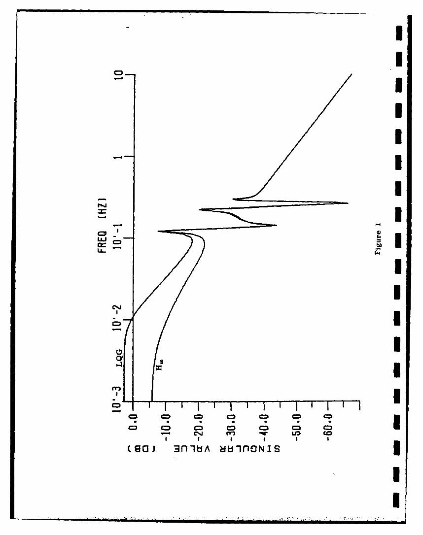
U13 co3nlU iunONI

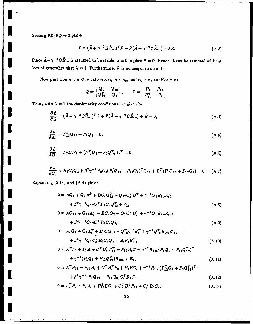
i Setting 1ClQ = 0 yields

1 0 = (A+ 1-2 Q/.)Tp + P(A+ Y-2 Qk ) + AR. (A.3)

Since A+-/- QkRo is assumed to be stable, A = 0 implies P = 0. Hence, it can be assumed without

loss of generality that A = 1. Furthermore, P is nonnegative definite.

Now partition ii x A Q,P into n x n, n x n., and n, x n, subblocks as

SQ 1 Q12 p PI P 2]

Thus, with A = 1 the stationarity conditions are given by

a1 = (A + Q I? ) p + p(A + . f?") + I = 0, (A.4)

Iz a Pe2 Q12 + P2Q2 = 0, (A.)

B' = P2 BcV 2 + (P1 Q, + P2 QT)CT = 0, (A.6)

812 = R2C.Q 2 + 32 - 2R 2C.(P;Ql2 + p 1 2 Q 2)TQ 12 + BT(P1 Q12 + P12Q2) =0. (A.7)

Expanding (2.14) and (A.4) yields

0 = AQ, + Q I AT + BC QT + Q 2 CTBT + -r 2 QR,RQl+ " C.Q + V1 , (A.S)

IS-rQ2C.YR 2C 12QA.8

0 = AQ 12 + Q12Ar + BC.Q 2 + Q1CTBT + -- 2 QR 1 .Ql 2

+ fl 2 - 2Q12C,,R 2C.Q 2 , (A.9)AQ2 + Q 2 AT + B.CQ1 2 + QCTBT +7 2 QTRQ 1 2

+,62- 2 Q2CTR2 CQ 2 + BcV B , (A.10)

0- ATP + PIA + CTB .,Y P + PI2 B.C + RlR c(PIQI + P1 2 q T2

+ <(p 1 QI + P 2Q?;)RI. + RI, (A.11)

0- ArP12 + P12A, + CTBTP2 + P1 BC. + - 1R,.(PT2Q, + p2QT)

I + 62 -i 2 (P1Q12 + P12Q2 )CTR 2C, (A.12)

0= ATP2 + P2 A. + Pj2 BCr + C BT P12 + CY:TR 2 C, . (A.13)

U 25I

Lemma A.1. Q2 and P 2 are positive definite.

Proof. By a minor extension of results from [40], (A.10) can be rewritten as 30 = (A. + B.CQ1 2Q2)Q 2 + Q 2 (A. + B.CQ12 Q+)T + T,

where

whr - 2 R1 Q 1 2 + , 2 _1- 2 Q2CTR 2CQ 2 + B.V2 Bm

and Qj is the Moore-Penrose or Drazin generalized inverse of Q2. Next note that since (Ac, B:) is

controllable it follows from Lemma 2.1 and Theorem 3.6 of [28] that (A, + BcCQ 1 2 Q2+, TI) is also

controllable. Now, since Q2 and T1 are nonnegative definite, Lemma 12.2 of [28] implies that Q2 is

positive definite. Using (A.13), similar arguments show that P 2 is positive definite. 0

Since R 2,V 2,Q 2 ,P 2 are invertible, (A.5)-(A.7) can be written as

-P:iP Q12 Q_1 = .., (A.14)

B. = -P; 1 (P 2 Q, + P2Q)CTv ", (A.15)

C"[I.. + 1- 2(qPI + Q2P 2)Ql 2Q21 ] = -R£lB(PQ 12 + P12Q2)Q2'. (A.16)

Now define the n x n matricesQ Q Q - Q Q Q, P p, - pp T2,

!' QQ P' P1" 2mj 2

-Q 12 Q 2 P 1P 2 ,

and the n, x n, n, x n. and n, x n matrices

GQ-IQ, M A ,, r A= _-1PITG~Q~ 1 2~ M Q2 P2 , r p; 1

2 _.

Note that r = GTr.m

Clearly, Q, P, 40 and P are symmetric and 10 and P are nonnegative definite. To show that Q

and P are also nonnegative definite, note that Q is the upper left-hand block of the nonnegative- m

definite matrix 7QQ, where

AA rIn -Q 12 Q21 10,n.Xn I.. I

Similarly, P is nonnegative definite.

26 m

I

I Next note that with the above definitions (A.14) is equivalent to (6.2) and that (6.1) holds.

Hence r - GT is idempotent, i.e., r 2 = r.

It is helpful to note the identities

I Q = Q 1 2 G = GTQT = GTQ2(, P = 2= rTP; = TTp2r, (A.17)

rGT = GT, Fr= r, (A.18)

Q = P = Pr, (A.19)

- -Q 1 2PT. (A.20)

Using (A.14) and Sylvester's inequality, it follows that

rank G = rank r = rank Q12 = rank P 12 = n,.

3 Now using (A.17) and Sylvester's inequality yields

n = rankQ12 + rankG-ne< rankQ_< rankQ12 =n,

which implies that rank = n,. Similarly, rank ? = n,, and rank QP = n, follows from (A.20).

U The components of Q and P can be written in terms of Q, P,Q, 5,G and r as

3 Q1 =Q+Q, P 1 =P+P, (A.21)

Q12 = ,,T, P1 2 -PGT, (A.22)

Q2 = VQF, P2 = GPGT. (A.23)

Next note that by using (A.21)-(A.23) it can be shown that the right-hand coefficient of C, in

I (A.16) is given by§ A 1.I,6+ 2 .7-2r2 PGT .

To prove that S is invertible use (A.19) and (6.3) and note that

3 I". + 01-1-2rQPGT = I. + #2 1-y3NrTPGT

= I.. + # 2 - 2 (rQrT)(GPGT).

Since r T and GPGT are nonnegative definite, their product has nonnegative eigenvalues (see

Lemma 5.1). Thus each eigenvalue of I, , +,6 2 y- 2 QPGT is real and is greater than unity. Hence3 S is invertible. Now note that by using (6.2) and (6.3) it can be shown that

GT§ -I = Sr.

SI27

The expressions (6.11), (6.12) and (6.13) follow from (A.15), (A.16), and the definition of Q. Next,

computing either I'(A.9)-(A.10) or G(A.12)+(A.13) yields (6.10). Substituting (A.21)-(A.23) into

(A.,S)-(A.13) and the expression for A, into (A.9), (A.10), (A.12) and (A.13) it follows that (A.10)

= P(A.9) and (A.13) = G(A.12). Thus, (A.10) and (A.13) are superfluous and can be omitted.

Thus, (A.8)-(A.13) reduce to

0 = AQ + QAT + V, + _Y-2 (Q + )R.(Q + (2}+ 2"7-2(STP.PS(

+ (A- EPS)Q + ((A - .PS)T, (A.24)

0 = [(A - _PS)Q( + (A - ZPS)T + QQ + -r 2(Q + 2)Rjo1 (Q + Y- -QRIIQ

+ #,-2r 2 ST p rps(]VrT, (A.25)

0 = (A + _- 2[Q + Q]Roo)TP + P(A + ,7-2 [Q + ]R 1 .) + R,

+ (A - Q2 + '- 2QR,.)Tp + /(A - Q2 + -'- 2QRoj), (A.26)

0 = [(A - Q,2 + -,-2QRoc,)Tfp + P(A - Q2, + "- 2QR10 ) + STPZPS]GT. (A.27)

Next, using (A.24)+GTF(A.25) G - (A.25)G - [(A.25)GIT and GTr(A.25)G - (A.25)G - [(A.25)GT

yields (6.5) and (6.7). Similarly, using (A.26)+rTG(A.27)r-(A.27)r-(A.27)r]T and

rTG(A.27)r-(A.27)r-[(A.27)r]T yields (6.6) and (6.8).

Finally, to prove the converse we use (6.5)-(6.13) to obtain (2.14) and (A.4)-(A.7). Let

Ac, Be, Cc, G,/r, r, Q, P, , P, Q be as in the statement of Theorem 6.1 and define Q 1, Q 12, Q2,

P1 ,P12,P 2 by (A.21)-(A.23). Using (6.2), (6.11) and (6.12) it is easy to verify (A.6) and (A.7).

Finally, substitute the definitions of Q, P, Q, 5, G, I', and r into (6.5)-(6.8) using (6.2), (6.3),

and (A.19) to obtain (2.14) and (A.4). Finally, note that I

Q [Q 0.,..] +[In] [rn pT I,

which shows that Q . 0. 0.

II

I_ .L_" . --- =""--== ==== ==m mm28'= a = U

I References

1. H. Kwakernaak and R. Sivan, Linear Optimal Control Systems, Wiley, New York, 1972.

2. G. Zames, "Feedback and Optimal Sensitivity: Model Reference Transformations, Multiplica-tive Seminorms, and Approximate Inverses," IEEE Trans. Autom. Contr., Vol. AC-26, pp. 301-320, 1981.

3. B. A. Francis and J. C. Doyle, "Linear Control Theory with an Ho" Optimality Criterion,"SIAM J. Contr. Optim., Vol. 25, pp. 815-844, 1987.3 4. B. A. Francis, A Course in Ho, Control Theory, Springer-Verlag, New York, 1987.

5. J. C. Doyle and G. Stein, "Multivariable Feedback Design: Concepts for a Classical/ModernSynthesis," IEEE Trans. Autom. Contr., Vol. AC-26, pp. 4-16, 1981.

6. B. A. Francis, "On Robustness of the Stability of Feedback Systems," IEEE Trans. Autom.Contr., Vol. AC-25, pp. 817-818, 1980.

7. I. R. Petersen, "A Riccati Equation Approach to the Design of Stabilizing Controllers andObservers for a Class of Uncertain Linear Systems," IEEE Trans. Autom. Contr., Vol. AC-30,pp. 904-907, 1985.

8. A. R. Galimidi and B. R. Barmish, "The Ccjstrained Lyapunov Problem and Its Applicationto Robust Output Feedback Stabilization," IEEE Trans. Autom. Contr., Vol. AC-31, pp. 410-419, 1986.

9. I. R. Petersen and C. V. Hollot, "A Riccati Equation Approach to the Stabilization of UncertainSystems," Ahtomatica, Vol. 22, pp. 397-411, 1986.

10. K. Zhou and P. P. Khargonekar, "Stability Robustness Bounds for Linear State-Space Modelswith Structured Uncertainty," IEEE Trans. Autom. Contr., Vol. AC-32, pp. 621-623, 1987.

11. D. Hinrichsen and A. J. Pritchard, "Stability Radius for Structured Perturbations and theAlgebraic Riccati equation," Sys. Contr. Lett., Vol. 8, pp. 105-113, 1987.

12. D. S. Bernstein and W. M. Haddad, "The Optimal Projection Equations with Petersen-HollotBounds: Robust Controller Synthesis with Guaranteed Structured Stability Radius," Proc.IEEE Conf. Dec. Contr., pp. 1308-1318, Los Angeles, CA, December 1987.

13. D. S. Bernstein, "Robust Static and Dynamic Output-Feedback Stabilization: Deterministicand Stochastic Perspectives," IEEE Trans. Autom. Contr., Vol. AC-32, pp. 1076-1084, 1987.

14. D. S. Bernstein and W. M. Haddad, "The Optimal Projection Equations with Petersen-Hollot Bounds: Robust Stability and Performance via Fixed-Order Dynamic Compensation forSystems with Structured Real-Valued Parameter Uncertainty," IEEE Trans. Autom. Contr.,Vol. AC-33, pp. 578-582, 1988.

15. D. S. Bernstein and W. M. Haddad, "Robust Stability and Performance for Fixed-Order Dy-namic Compensation via the Optimal Projection Equations with Guaranteed Cost Bounds,"Proc. Amer. Contr. Conf., pp. 2471-2476, Atlanta, GA, June 1988.

16. D. S. Bernstein and W. M. Haddad "Robust Stability and Performance Analysis for LinearDynamic Systems," submitted.

17. J. C. Doyle, "Analysis of Feedback Systems with Structured Uncertainties," lEE Proc.,Vol. 129, pp. 242-250, 1982.

18. I. R. Petersen, "Disturbance Attenuation and H' Optimization: A Design Method Based onthe Algebraic Riccati equation," IEEE Trans. Autom. Contr., Vol. AC-32, pp. 427-429, 1987.

19. P. P. Khargonekar, I. R. Petersen, and K. Zhou, "Robust Stabilization of Uncertain Systemsand H' Optimal Control," preprint.I

I. .. .• w . m' | ! ! I . ! ||. .|

I

20. D. C. Hyland and D. S. Bernstein, "The Optimal Projection Equations for Fixed-Order Dy- Inamic Compensation," IEEE Trans. Autom. Contr., Vol. AC-29, pp. 1034-1037, 1984.

21. D. A. Wilson, "Convolution and Hankel Operator Norms for Linear Systems," preprint. 322. M. J. Grimble, "Optimal H,, Robustness and the Relationship to LQG Design Problems,"

Int. J. Contr., Vol. 43, pp. 351-372, 1986.

23. M. Mariton and R. Bertrand, "A Homotopy Algorithm for Solving Coupled Riccati Equations," 3Optim. Contr. AppL. Meth., Vol. 6, pp. 351-357, 1985.

24. S. Richter, "A Homotopy Algorithm for Solving the Optimal Projection Equations for Fixed-Order Dynamic Compensation: Existence, Convergence and Global Optimality," Proc. Amer.Contr. Conf., pp. 1527-1531, Minneapolis, MN, June 1987.

25. S. W. Greeley and D. C. Hyland, "Reduced-Order Compensation: LQG Reduction VersusOptimal Projection Using a Homotopic Continuation Method," Proc. IEEE Cnf. Dec. Contr., Ipp. 742-747, Los Angeles, CA, December 1987.

26. J. C. Doyle, K. Glover, P. P. Khargonekar, and B. A. Francis, "State-Space Solutions toStandard H2 and Ho Control Problems," Proc. Amer. Contr. Conf., pp. 1691-1696, Atlanta,GA, June 1988.

27. A. N. Madiwale, "Some Practical Aspects of H,, Compensators," MIT Lincoln Laboratory, inpreparation.

28. W. M. Wonham, Linear Multivariable Control: A Geometric Approach, Springer-Verlag, NewYork, 1979. 3

29. J. C. Willems, "Least Squares Stationary Optimal Control and the Algebraic Riccati Equa-tion," IEEE Trans. Autom. Contr., Vol. AC-16, pp. 621-634, 1971.

30. R. W. Brockett, Finite Dimensional Linear Systems, Wiley, New York, 1970. 331. K. Glover, "All Optimal Hankel-Norm Approximations of Linear Multivariable Systems and

Their L°-Error Bounds," Int. J. Contr., Vol. 39, pp. 1115-1193, 1984.

32. D. S. Bernstein, "The Optimal Projection Equations for Static and Dynamic Output Feedback:The Singular Case," IEEE Trans. Autom. Contr., Vol. AC-32, pp. 1139-1143, 1987.

33. A. Bensoussan and J. H. van Schuppen, "Optimal Control of Partially Observable StochasticSystems With an Exponential-of-Integral Performance Index," SIAM J. Contr. Optim., Vol. 23, Ipp. 599-613, 1985.

34. D. H. Jacobson, Extensions of Linear-Quadratic Control, Optimization and Matrix Theory,Academic Press, London, 1977.

35. P. Whittle, "Risk-Sensitive Linear/Quadratic/Gaussian Control," Adv. Appl. Prob., Vol. 13,pp. 764-777, 1981.

36. C. R. Rao and S. K. Mitra, Generalized Inverse of Matrices and Its Applications, John Wileyand Sons, New York, 1971. 1

37. A. J. Laub, "A Schur Method for Solving Riccati Equations," IEEE Trans. Autom. Contr., iVol. AC-32, pp. 913-921, 1979.

38. R. H. Cannon, Jr., and D. E Rosenthal, "Experiments in Control of Flexible Structures withNoncolocated Sensors and Actuators," AIAA J. Guid. Contr. Dyn., Vol. 7, pp. 546-553, 1984.

39. Y. Liu and B. D. 0. Anderson, "Controller Reduction via Stable Factorization and Balancing,"Int. J. Contr., Vol. 44, pp. 507--531, 1986.

40. A. Albert, "Conditions for Positive and Nonnegative Definiteness in Terms of Pseudo Inverse,"SIAM J. Contr. Optim., Vol. 17, pp. 434-440, 1969. I

I,, . - , ,.... - ,:... ; .,. . .; ,,. " , .. •. . . ...

I

I 41. D. S. Bernstein and W. M. Haddad, "LQG Control with an H,, Performance Bound: A RiccatiEquation Approach," Proc. Amer. Contr. Con!., pp. 796-802, Atlanta, GA, June 1988.

42. H. Kwakernaak and R. Sivan, "The Maximally Achievable Accuracy of Linear Optimal Reg-ulators and Linear Optimal Filters," IEEE Trans. Autom. Contr., Vol. AC-17, pp. 79-86,1972.

I'I.IIIIIIIIIIIIII---• i I I I I

ROBUST 6II CONTROL DESIGN FOR SYSTEMS WITH STRUCTURED PARAMETER LNCERTAINTY

Appasaheb N. M!adiwale Wassim M1. Hladdad Dennis S. Bernstein**Lincoln Laboratory/M.I.T. Florida Institute of Technology Hlarris CorporationP.D. Box 73 Mfelbourne, FL 32901 P.O. Box 37

Lexington, MA 02173 Melbourne, FL 32901

Abstract flexibility. Extensions to even more general designproblems are mentioned in Section 9 but omitted here

In a recent paper a unification of the L2 (LQG) for lack of space.and Hm control design problems was obtained in terms ofU modified algebraic Riccati equations. In the present Notation. Note: All matrices have real entries.paper these results are extended to guarantee robust L2and Hm performance in the presence of structured real- R, Orxs, Rr, E real numbers, r x s real matrices,valued parameter variations (AA, AB, AC) in the state RrxI, expected valuespace model. For design flexibility the paper con-siders two distinct types of uncertainty bounds forboth full- and reduced-order dynamic compensation. An r x s zero matrix, Orx aimportant special case of these results generates Lcontroller designs with guaranteed gain margins. Sr4Nr Pr r x r symmetric, nonnegative defi-

nite, positive-definite matrices

I. Introduction Z1 Z2 , Z1 < Z2 Z2 - Z r, Z2 - Z, [pr,

It has recently been shown that the solution to ZI; Z2 Sr

* the optimal Hm disturbance attenuation problem can be positive integersexpressed in terms of a pair of modified Riccati equa-

tions ([1,2]). Furthermore, it was shown in [1] that p,dc,q,qm; i positive integers; n + nc (nc < n)L2/Hw design tradeoffs can be achieved by solving a

* coupled system consisting of three modified Riccati x-uly'xcR n,m,t,nc, fi-dimensional vectorsequations. As is well known, the disturbance attenua-tion problem can be used to guarantee robustness with A,AA; B,AB; C.AC n x n; n x m; t x n matricesrespect to unstructured plant uncertainties. However,if plant uncertainty is present in the form of para- Ac. Bc, Cc nc x nc, nc x t, m x nc matricesmetric variations of the state space model, then alter-native bounding techniques are required. The goal of xj f A BCc 1c fAA ABCC1the present paper is thus to extend the results of [1] R, A, ij [ [U C BA [cAC 0to include bounds on the effect of real-valued struc-tured parameter variations. 4) d-dimensional standard white noise

In the absence of an Hf design constraint, robust rstability and L2 performance for dynamic compensator D.Dnxd, xdmtie:DID2 =0design were guaranteed in [3.41 by incorporating quad-ratic Lvapunov bounds within LG design theory. Two D T n D d .da ;distinct bounds were considered. In t3] a quadratic VT. V1 DiD1 , '2 E

bound was used while in [4] a linear bound was em-ployed. In each case full- and reduced-order dynamic [D 1 1 r V, Onxfc 1compensators were characterized by means of coupled j.systems of modified Riccati and Lyapunov equations. D2 , ncXn BcV2BJ

To design ff controllers which are robust with re-* spect to structured real-valued parameter variations we

proceed by combining the results of [1] with those of E2 q x n. q x m matrices; E E2 0[3.4]. That is, we derive coupled systems of modifiedaiccati and Lvapunov equations whose solutions yield E, R . R, [El E2C¢] . EE. EE2 ; R2 PmI controllers which are guaranteed to satisfy a prespeci- - 2

fied H16 attenuation constraint for all variations (AA,All, AC) belonging to a $iven uncertainty set. If the [ R, Onfxnc

uncertainty is absent (i.e., AA = 0, etc.) then the re- R I EnCsults of [I] are recovered, while if the H constraint Onc., C~R2 Cc

U is relaxed, then the results of [3.4] are obtained.Thus the results of [1] can be viewed as a specializa- E0. Ex qo x n. qx x m matrices,tion of a broader design theory which accounts forstructured real-valued parameter uncertainty. Finally, T

* we state all results for the case of a fixed-order ElE 20 0

(i.e., reduced-order) controller for maximal design

I This work is sponsored by the Dept. of the AirForce. The views expressed are those of the author and -Rim Onxncdo not reflect the official policy or position of the TU.S. Government. "Oncxn CCR 2xCj** Supported in part by the Air Force Office ofI Scientific Research under contract F49620-86-C-0002.

ID1GO, D2' n x dw, I x dw matrices; D,'D 2 0 (iii) the performance functional

V1®, V2 T DaDT®, D Dr J(Ac,BC,CC) = sup lim sup U2 2J2 (AA, AB, AC)eU t - 0

D "1 xcj E[XT(t )Rlx(t) + UT(t)R2U(t)1 (2.7)

D20 . ncxn BcV 2 BcT I is minimized.

3, 7, a nonnegative constant; positive Note that for each uncertain variation (AA, AB,constants AC) c U, the closed-loop system can be written as I

A0, Aca A + I,9 Ac + - In. i(t) = (A + AA)R(t) + Dw(t), tf[O.W), (2.8)and that (2.7) becomes

II. Robust Stability and L, Performance with J(Ac,Bc,Cc) sup lim supa Robust Hll Constraint (AA, AD, AC)fU t -

In this section we state the Robust stability and E[iT(t)f()L2 performance problem with robust Ho disturbance at- E( 2.9)tenuation constraint. Specifically, we consider afixed-order dynamic output-feedback control-design Note that the problem statement involves both L Uproblem with structured real-valued plant parameter and Ho performance weights. In particular, the matri-uncertainties and constrained Ha disturbance attenua- ces R, and R2 are the L2 weights for the state and con-tion. This problem involves a set U c IRnxn x Rnxm x trol variables. By introducing the variablesRkxm of uncertain perturbations (AA, AB, AC) of thenominal system matrices (A, B, C). The goal of the z(t) = Eix(t), v(t) = E2u(t). Iproblem is to determine a fixed-order, strictly properdynamic compensator (Ar, Bc, Cc) which (a) stabilizes the cost (2.7) can be written asthe plant for all variations in U, (b) satisfies an Hwconstraint on disturbance rejection for all variations J(Ac, Bc, Cc) = sup lim supin U, and (c) minimizes the worst-case value over the (AA, AD, AC)fU t - Iuncertainty set U of a stead state L2 performance cri-terion. In this and the following section no explicit E[zT(t)z(t) + vT(t)v(t)].structure is assumed for the elements of U. In Sec-tions 4 and 7, two specific structures of variations in A T A TU will be introduced. For convenience we thus define R, = E1E, and R2 = E2E2

- Constrained Robust Dynamic Compensation Pro- which appear in subsequent expressions. Although an L2hbem. Given the nth-order stabilizable and detectable cross-weighting term of the form 2x (t)R,2u(t) can also 3plant with structured real-valued plant parameter var- be included, we shall not do so here to facilitate theiations presentation.

For the 113 performance constraint, the transfer 3.t = (A + AA)x(t) + (B + AB)u(t) + Dw(t). (2.1) function (2.5) involves weighting matrices E1 x and E2 x

y(t) = (C + AC)x(t) + D2w(t). (2.2) for the state and control variables. The matrices RO

determine an ncth-order dynamic compensator = EIM E x and R2x - E2X E2 are thus the Hx counter- 3parts of the L, weights R, and R2. Although we do not

xc(t) = Acxc(t) + Bcy(t) (2.3) require that R1T and R2x be equal to R, ana R2. weshall require that R2x = 32R 2. where the nonnegative

u(t) = Ccxc(t), (2.4) scalar 3 is a design variable. We further note that 3which satisfies the following design criteria: the assumption EOCE20 = 0 precludes an H cross-

weightin- term which again facilitates the presenta-1i) the closed-loop system (2.1) - (2.4) is asymptot- tion. Finally. similar remarks apply to the distur-

ically stable for all (AA, AD, AC; f U , i.e., + Ai bance and sensor noise intensities V 0 DT. Vis asymptotically stable for all (AA, AB. AC) E U: 1 2Ordy DD

2' 0 .0, T 2 2

T for the [, and lix(ii) the qx x d closed-loop transfer function 020, O and V23 O Xdesigns respectively. We note that w(t) can be inter-

E®[sI- -(A + AA)]'D, (2.5) preted as white noise for the L, design aspect and asAi(s) x n an L2 signal for the Hx design aspect [I].

from w(t) to Etmx(t) + E-2 u(t) satisfies the con- Before continuing it is useful to note that ifstraint (A + AA) is asymptotically stable for all (AA. AB. AQC)

c U for a given compensator (A. Be, Cc) then the per-JJlli(s)J[x 5 7, (AA, AD, AC)cU, (2.6) formance (2.7) is given by

where 7 > 0 is a given constant; and II

J(Ac, Bc, Co) = sup tr QA, (2.10) solution to (2.14). Now for (6A, AB, AC) c U, (2.14)3 (AA, AB, AC) U is equivalent to

where the steady-state closed-loop state covariance de- 0 = (A + AA)Q + Q(A + AA)T + 7-2 QkQfined by + fl(BC, Cc, q) -(AAQ + qAF) + V. (2.21)A TI = lim E[:(t)i(t)], (2.11) Hence, by assumption, (2.21) has a solution Q e (Nn for

t --. all (AA, AB, AC) c U and, by (2.13), 0 (Be, Cc, Q)-(AAQ + qAir) is nonnegative definite. Now if the sta-

satisfies the fi x fi algebraic Lyapunov equation bilizability condition (2.15) holds for all (AA, AB,

AC) e U, it follows from Lemna 12.2 of [5] that A + Al0 = (A AI)QA + QA( + AA)T + V. (2.12) is asymptotically stable for all (AA. AB, AC) f U.

Conversely, if A + AA is asymptotically stable for allThe key step in uaranteeing robust stability and (AA, AB, AC) f U, then (2.15) holds. The proof of

performance is to replace the uncertain terms in the (2.17) now follows from a standard manipulation ofcovariance Lyapunov equation (2.12) by a bounding func- (2.14 . Next, subtracting (2.12) from (2.20) yields

I tion 0. Note that since AA is independent of Ac, the

bounding function il need only depend on Bc and Cc. 0 = (A + AA)(Q -1AA) + (Q - + AA)T + 7"2qfq

Furthermore, the H® constraint (2.6) on the disturbanceattenuation is enforced for all (AA, AD, AC) e U by re- + 0 (Be, Co, I) -(AAQ + qAAT)E placing the modified algebraic Lyapunov equation (2.12)by an algebraic Riccati equation which overbounds the or, equivalently, since A + Ai is asvmptotically stableclosed-loop steady-state covariance. Justification for for all (AA, AB, AC) c U,this technique is provided by the following result.

Lemma 2.1. Let 9: Rncx/ x Rmxnc x N; - S; be U -h e(" + A)t [7-2 Q RX q + fl (BC, Cc, q)

such that -(AAQ + QAAT)]e(' + AA) Tt dt 0

AAQ + rJAjT < Q(Bc, Cc, Q); (AA, AB, AC)fU, which implies (2.18). The performance bound (2.19) is

(Bc, Cc, q)fRtcXix Rxnc x W, (2.13) now an immediate consequence of (2.18). c

Remark 2.2. Note that (2.15) is actually aand, for a given (Ar, Bc, Ce), suppose there exists closed-loop "disturbability" condition which is notq f N satisfying concerned with control.as such. This condition guaran-

tees that the closed-loop system does not possess un-

T stable undisturbed modes. In applying Lemma 2.1 it may0=iq + qA + 7"2qI q + J2(Bc, Cc, q) + V, (2.14) be convenient to replace condition (2.15) with a

then stronger condition which is easier to verify in prac-tice. Clearly. (2.15) is satisfied if [V + . -2 QRXQ

(A + A, [V + 7 -2q#.q + R(B, Cc, Q) -(AAQ + qAAT)]J) + 9 (Bc, CC. q) -(AA q + q AAT)h is positive definitefor all (AA. AB, AC) c U. This will be the case, for

is stabilizable for all (AA, AB, AC)cU. (2.15) example, if either V is positive definite or strict in-equality holds in (2.13). Also, it follows from Theo-

if and only if rem 3."of [5] that (2.15) is implied by the stronger

condition thati + AA is asymptotically stable, (AA, AB, AC)cU (2.16)

In this case, (A + AA, D) is stabilizable. (AA, AB. AC)cU. (2.22)

I1HAA(s)11 < 7, (AA, AB, AC)cU, (2.17) Ili. The Auxiliary Minimization Problem

and As shown in the previous section. the replacement-of (2.12) by (2.14) enforces the Ho disturbance atten-

_ ~q, (AA, AB, AC)cU, (2.18) uation constraint and yields an upper bound for theworst case L2 performance criterion. That is, given acompensator (Ar, Bc, Cc) for which there exists a non-

where Qa is given by (2.12). Consequently, negative-definite solution to (2.14), the actual worstcase L2 performance (Ac, B', Cc) of the compensator is

J(Ac. Bc, Cc) < J(Ac. Be, Cc, Q), (2.19) guaranteed to be no worse than the bound given byJ (Ac, Be, Cc, Q). Hence, J (At, Bc, Cc. 9) can be in-

where terpreted as an auxiliary cost which leads to the fol-D lowing optimization problem.

J(AC, De, Co, Q) A tr QR. (2.20) Auxiliary Minimization Prohlem. Determine (Ac,Bc, Cc, Q) which minimizes J (Ac. Bc, Cc, Q) subject to

Proof. First note for clarity that in (2.13) Q (2.14) with Q c N;.

denotes an arbitrary element of Wn since (2.13) holds It follows from Lemma 2.1 that the satisfaction offor all Q f N". while in (2.14) Q donotes a specific (2.14) for Q c ; along with the generic condition

........ ..I- ~ a l i m | |I i

(2.15) leads to 1) closed-loop stability for all (AA, right shift of the open-loop dynamics. The second termAD, AC) e U; 2) prespecified H performance attenuationfor all (AA, AD, AQC) U; and 3) an upper bound for the a- 0 2AiQAT arises naturally from a multiplicativeworst case L2 performance criterion. Hence, it remains I Ito determine (Ac, BD, Cc) which minimizes J (Ac, BC, white noise model. Such interpretations have no bear-Cc, Q) and thus provides an optimized bound for the ac- in- on the results obtained here since, only the boundtual worst case L2 performance J (Ac, Be, Cc) over all Q1 aefined by (4.3) is required. We call (4.3) the 3

(AA, AB, AC) e U. linear bound since it is linear in q. For a more de-tailed discussion on (4.3) see [4].

IV. Uncertainty Structure: Linear Bound With l defined by (4.3), the modified Riccati

Having established the theoretical basis for our equation (2.14) becomes

approach, we now assign explicit structure to the set U = ,qT,- (4)and bounding function f Specifically, the uncertainty 0= XQ qV + 7 2Q#_q + aQ + a - afAiqA: + V (4.4)set U is assumed to be of the form i1 i

P or, equivalently,

U = {(AA, AD, AC): AA = EiAi, AD = ,oiBi,

0 q O X + qi T + 72 Qk.Q+ 6XiiT + V, (4.5)

AC , 0/a < 1}, (4.1)

where, for i 1, ... , p: Ai c Rnx, Bi e Rnxm, and Ci where i A a 2/& and 3f RJxn are fixed matrices denotin& the structure of theparametric uncertainty; ai is a given positive number; - [A BC,and ai is an uncertain real parameter. Note that the A A + = iuncertain parameters oi are assumed to lie in a speci- a 2 LBcC Acfied ellipsoidal region in RP. The closed-loop system(2.8) thus has structured uncertainty of the form V. Sufficient Conditions for Robust Stabilitv

and Performance with Robust Hm Disturbance

AA = uiAi, (4.2) Attentuation: Linear Bound 3i1 In this section we state sufficient conditions for

characterizing fixed-order (i.e., full- and reduced-where order) controllers guaranteeing closed-loop stability 3

C icfor all (AA, AC) f U, constrained Hm disturbance atten-S]; i= 1 .... , P" euation for all (AA, AC) c U, and an optimized worst

BCC 01P case L2 performance bound.

In order to state the main results we require some 3Note that tie symmetry of the uncertainty set entails additional notation and a factorization lemma.no loss of generality by requiring only a redefinitionof the nominal plant matrices.

Lemma 5.1. Let Q, P c Nn and suppose rank QP = n, UIn order to obtain explicit gain expressions for then there exist n, x n G, r and nc x n, invertible M1.

(Ac. Bc, Cc) in Sections 5 and 6, we shall require that unique except for a change of basis in -nc, such thatat most one of the perturbations AB and AC is nonzero.We thus consider the cases (AA. AC) f U or (AA, AB) f mU. If this assumption is not imposed, then optimality QP = CTMr. rGT = I"nC- (5.1), (5.2)conditions can still be derived, but at the expense ofclosed-form gain expressions. In this section, and Furthermore. the nxn matricesSection 5 we will assume that AR = 0 (i.e., Bi = 0, i =1, ..., p) and fl (Be, Cc, Q) becomes fl (Be, Q). The AAdual case AR # 0, AC = 0 (i.e., Ci = 0, i = 1, ..., p) r = G r, r = In -r (5.3), (5.4)will be considered in Sectiop 6.

are idempotent and rank n, and n -nc, respectively.For the structure of U specified by (4.1), the Finally, if P f n and 3 > 0 then the inverseI

bound Q1 satisfying (2.13) can now be given a concreteform. S 4 (I1 + 27 2 P)- l (5.5)

Proposition 4.1. Let a be an arbitrary positivescalar. Then the function exists. 3

4 + - 2 (4.3) For arbitrary Q, nxn and a > 0 define theQ(110, q) Q a 'l § a2AiAT4. following notation:

satisfies (2.13) with U given by (4.1) and AR = 0. V2 + E 6iCi(Q + O)C,i'1

Proof. See [4]. oAS QC+Zb~( + Q i E A R 1 r

Remar 4.1. Note that the bound fl given by (4.3) 1

consists of two distinct terms. The first term aQ canbe thought of as arising from an exponential timeweighting of the cost, or, equivalently, from a uniform 3

Suppose there exist Q, P, P Remark 5.2. To specialize Theorem 5.1 to the fullsatisfyig order case nc = n, it is only necessary to set GT = r-_

T so that G = r = r = I,, and r = 0 without loss of gen-

0 A a + 7-2 QRQ + Vt erality. Now the last term in each of (5.6) - (5.9)P can be deleted and G and r in (5.11) - (5.14) can be

+ E ..A.(Q + Q)AT - QV2 I q + r Q$V T (5.6) taken to be the identity. It is interesting to note6 that in the full-order case the Hw design problem withstructured parameter variations is comprised of four

a + 1-2[o +4]RI )Tp - P(A + 7-2[+ Q R , coupled Riccati/Lyapunov equations. Thiq coupling(A 0 a IQ + QJR1)D illustrates the breakdown of reulator/estimator sep-

A Aration and shows that the certainty equivalence prin-P + (Ai -sV2;lCi)TP(Ai -sV 2 'Ci)] ciple is no longer valid. This is not surprising sincei P separation also breaks down for the full-order L2 re--STPEPS + TTSTPEPSr, (5.7) sult with parameter uncertainties [4].

Remark 5.3. When solving (5.6) - (5.10) numeric-

0= (A a-EPS + 7-2QR Q + Q(A -S + 7 + ally, the uncertainty terms and the I16 constraint can

a )Q +( 7 2QR +,) be adjusted to examine tradeoffs among performance,7-2 + 2STpIpS)Q + I qT _7 ... TT (.5.8) robustness, and disturbance rejection. Specifically,

SQ V2s rs v2s Isr,( the uncertainty range ai and the structure matrices Ai,Ci appearing in Qs and V2s along with 7 can be varied

A+-2QRI )Tp + A 1C systematically to determine the region of solvabilityS(A a -QsV2 l + 7- 00) a A - 2S of the design equations (5.6) - (5.9).I+ r7"2QRt® + sTpEPS -rTSVP PSr, (5.9)

R Remark 5.4. Although equations (5.6) - (5.10)

appear formidable, they are, in fact, quite numericallytractable. For related problems involving coupled

rank Q rank P = rank nc, (5.10) Riccati equations, homotopic continuation methods havebeen shown to be effective (see [I] and the References

and let (Ac, Be, Cc, Q) be given by therein).A= r(A -Ues -QsV 2 C + 7-2QR )GT (5.11) Remark 5.5. We point out that if 0 or, equiv-S=, Icalently, E2. = 0, which corresponds to the "cheap" Hm

control case (i.e., H® attenuation between disturbancesBc = rQsV2;1, (5.12) and controls is not constrained), it is possible to ob-

tain closed-form gains (A,, Be, Cc) given by a modified-T T set of design equations when all three of AA, AB, and

Cc = -PB PSGr, (5.13) AC are nonzero. Because of space limitations this re-sult will be given in a future paper.

Q q Q + Q Qr" TT1. Remark 5.6. An important special case of the re-Urq rqr sults of Section 5 is obtained bv setting AA = 0,

AB = 0, AC = aC1 , and C1 = C. The resuiting L2/ll

Then. (A + AA, D) is stabilizable if and only if A + AA design possesses guaranteed gain margin of *100a per-

is asymptotically stable for all (AA, AC) c U. In this cent at the sensor output.case,.the closed-loop transfer function HA(s) satis-

fies the B1 disturbance attenuation constraint VI. The Dual Case: Linear Bound

7, Unlike the standard LQG result involving a pair ofuncoupled Riccati equations, the new result uarantee-

and the worst case L2 performance criterion (2.10) ing robust stability, robust performance, and distur-adt ewst h e n pbance rejection involves a coupled system of four modi-satisfies the bound fied Riccati/Lyapunov equations. The asymmetry of

these equations suggests the possibility of a dual re-J(Ac, Bc, Cc) tr[(Q + Q)R1 + QS

TPtPSQ]. (5.16) sult in which the modifications to the standard Riccatiequations are reversed. One motivation for developing

Proof. The proof follows from Lemma 2.1 by com- such dual results is that for certain problems the dualbinin the proofs of Theorem 6.1 of [1] and Theorem 6.1 bounds may be sharper than the primal bound introducedof [4T. a in Section 4. Furthermore, the dual theory permits

Rf[ emark 5.1. Theorem 5.1 presents sufficient con- we now requre R = R2. Finally, the dual theory

ditions for designing controllers yielding robust sta- 1

bility and performance with a constraint on the H11 norm allows for uncertainty in the control matrix B (i.e.,of the closed-loop transfer function for a state-space AB # 0). Although we now require AC = 0, (i.e., Ci =

system with structured real-valued plant parameter var- 0, i = 1, ... , p to obtain closed-form gain expres-iations. These sufficient conditions comprise a system sions for (Ar, Bc, Cc). We begin with the followingof three modified Riccati equations and one modified lemma:Lyapunov equation coupled by the optimal projection r,the linear uncertainty bound, and the HaI constraint. Lemma 6.1. Suppose the system (2.8) is asymptoti-

I lf the uncertainty bound is deleted, then the results cally stable for all (AA, AB, AC) cU for a given (Ac,of [1] are recovered. If, alternatively, the uncer- Bc, Cc). Thentainty terms are retained but the If6 constraint issufficiently relaxed, i.e., 7 - , then the results of J(Ac, Be, Cc) = sup tr PAAV, (6.1)[4] are recovered for the case Di = 0, i = p, ... , P (AA. AB, AC)cU

where PAA e N is the unique solution to 0 = (Aa * -2V1 [P + P])Q + Q(Aa + 7-2Vt1 P P])r

0= (A + AA)T P PA(A + AA) +R (6.2) + V1 + i E 6j[AiQAi + (Ai -BjRiP,)Q(A1 -BiR P)T] 3Proof. See [3]. o+ T SQEQ T , (6.10) 1

Utilizing (6.1) in place of (2.10), the H® distur- _-(A .bance attenuation constraint from plant and sensor dis- 0 a + 7-2V10p)P + P(A a -SQ + -7-2VLP) +

turbances to the Qtnte and control variables given by 7 12.(V1 + p:Q Qgr) + pIR~p8 _I pIp s r±,

IHAA(s)II1 = AIE[sl -(A + AA)]"1ljf 7 (6.3) 10 = (Aa -BR.lP, + 7-2V P)Q + Q(A -BRsPs + 72VMP)T

can now be enforced by replacing (2.14) by the modified + qtq T - 7r E£QST, (6.12) IRiccati equation I (6.12

0 = jAp + pA + 7 -2p ®p + (Cc, P) + and let (Ar, Bc, Cc, P) be given by

(AA, AB, AC)EU, (6.4) Ac = r(A -SI] -BRjP s + 7-2V, P)GT , (6.13) 3

where B= rSqCTVi , (6.14) n

AAP + pAj < f(C', p), (AA, AB, AC)eU. (6.5) UNote that (6.4) is merely the dual of (2.14). We also Cc = -R2PsGT , (6.15)

require the condition dual to (2.15) given by

[+ 7-2 pvp + f(Cc, p) -(Aj Tp + Pi)], A + )P P -PG (6.16)' i-o GPGTJ

is detectable for all (AA, AB)U. (6.6) Then, + AA) is detectable if and only if + AA.

For the structure of U as specified by (4.1) with is asymptotically stable for all (AA. AB) c U. In this

AC = 0, the bound fl satisfying (6.5) can now be given a case. the closed-loop transfer function Ri(s) satis-concrete form. fies the Hm disturbance attenuation constraint,

Proposition 6.1. Let a be an arbitrary positivescalar. Then the function 11Aji(s)JI. 5 7, (AA, AB)fU, (6.17)

)A a , TpT and the worst case L2 performance criterion (6.1) Nfl(Cc. P) oP + a" E P(6.7) satisfies the bound

satisfies (6.5) with U given by (4.1) and AC = 0. with (Ac, Bc, Cc) tr[(P + P)Vj + P Q ST ]. (6.18) 3l defined by (6.i). the modified dual Riccati equation Remark 6.1. The dual case of Remark 5.6 is obtained by(6.4) becomes setting AA = 0, AB = aBj, AC = 0, and B1 = B. The re-

sulting L2/IIx design possesses guaranteed gain margin *0 = A;P + PAa + 7"2PV=P + E 6.A PA1 + I

" (6.8) of ±100o.percent at the input.

We can now state sufficient conditions for robust VII. Uncertainty Structure and Sufficient Conditions

stability, robust L2 performance, and robust distur- for Robust Stability and Performance with Hm

bance attenuation for the dual problem. For arbitrary Disturbance Attenuation: Quadratic Bound

Q, P, P flRnxn and a > 0 define the following notation: We now assign a different structure to the uncer-tainty set U and the bounding function fR. Specifi- U

R2 T +cally, the uncertainty set U is assumed to be of the UR2s R2 6iBi(P + P)Bi, PsBP + E 6iB (P + P)Aj, form'

il i=J

(II -+ CTV-' IC.S (I2 + 7 2QP), E -

" U = {(AA. AB, AC): AA = I FiMiNiGii ~Z

Theorem 6.1. Suppose there exist P. Q, F, U e nD FiM 1NHi, AC = P NiMlNiG,

satisfying (5.10) and P-

P M1 IM i , N TNi Ni i = 1 .... p), (7.1)0 = AP + PA + 7 -2PV P + R + E b.A T(P + P)A i

1

prps+ rp.,rp , (6.9) where, for i = 1. p: Fi Rnxri, G, . ptixn=1li f tixI, and Ki c RIxri are fixed matrices denoting

the structure of the uncertainty: Mi f Nri and Ni c I"I

Ill nmu n nml~lilllllN

are given uncertainty bounds; and Mi e Rrixsi and and let Q be given by (5.14) and (Ac, Bc, Cc) by

i e RjXti are uncertain matrices.

In order to obtain explicit gain expressions (Ac, , = r(A -EPS -QaViaC + Q[7-2R. + E]), (7.9)

Bc, Cc) we again consider two cases, l)(AA, AC) f U Bc = rQv-, (7.10)S with AB = 0 and 2)(AA, AB) c U with AC = 0. When a,AB = 0 the closed-loop system has structured uncer-tainty of the form CT = P~jB TPSCT (7.11)

C. = k' PS

I i,(7.2) Then. (A + AA. D) is stabilizable if and only if A + AAI is asymptotically stable for all (AA, AC) c U. In this

where, case, the closed-loop transfer function lfAi(s) satis-fies the H, disturbance attenuation constraint

'K , [C 0]. 11 Ai(s)Jm S , (AA, AC) e U, (7.12)

In this case the quadratic bound Q satisfying (2.13) and the worst case L2 performance criterion (2.10) sat-

can now be given a concrete form. isfies the bound

Proposition 7.1. The function J(Ac, Bc, Cc) tr[(Q + Q)R, + QSTPEPSQ]. (7.13)

' (Proof. The proof follows by combining the proofsfl(Bc,, q) Fi1iFiT + GNGq(7.3) of Theorems 6.1 of [1] and Theorem 8.1 of '[3]. o

Remark 7.2. It is interesting to note that thesatifies (2.13) with U given by (7.1) and AB = 0. full-order case nc = n with G = r = r = In and r =0

Proof. See (3]. o (see Remark 5.1), P plays no role so that (7.8) issuperfluous. Thus, unlike the full-order result for

Thus, with f9 defined by (7.3), the modified the linear bound involving four equations, the full-Riccati equation (7.3) becomes order quadratic bound involves three modified Riccati

equations coupled by the uncertainty term and the Ho0 = Aq + qAT + 7-2 Q&Q + V constraint. If, alternatively, the reduced-order con-

straint is retained, but the uncertainty terms are de-+ Cij + O TNGq] leted, then the results of (1] are recovered. If,

+ E i (7.4) furthermore, the uncertainty terms are retained, butthe ll1c constraint is sufficiently relaxed, i.e.,

For arbitrary Q e Rnxn define: 7 - w, the results of [3] are recovered.

QA qCT + PFi i D A TF FT , VIII. The Dual Case: Oiadratic Bound

i iFor the structure of U as specified by (7.1) withS+ T, -TR AC = 0, the closed-loop system has structured uncer-V Ki %i Ki E E i G iGi. A ,tecoe-opsse a tutrducr

V2a i+- tainty of the form

Theorem 7.1. Suppose these exist Q, P, Q, P AA= E FiMiNiGi. (8.1)satisfying (5.10) and

0 = AQ + QA T + 72QRQ + V, + QEQ + D where

r a + V Ua, (7.5) P Fi d [Gi H1C,].

* 0 =(A + + 2]R, 001 + E]) TP Proposition 8.1. The function

+ P(A + [Q + ][7-2R,. + El) A(C P) - ,+ - P

+ R, S1 P ZPS + rT, (7.6) i+ s

satisfies (6.5) with U given by (7.1) and AC = 0.

-p With Q defined by (8.2), the modified dual equa-

+ [7-2 R1 + E]) + Q(7 [R + 2STPEPS] + E)O tion (6.4) becomes

+ .jq T T

U aV - a a (7.7) 0 = ATP + PA + 7 -2PV iP + ft

(A QaViAC + Q(7-2R,. + E] + A -QaV+aC i+P (8.3)

+ Q[7-2 R,® + E]) + STPEPS -rTSTPEPSr , (7.8)

I

I

For arbitrary P e Raxn define: 3) nonstrictly proper plant model, i.e., (2.2)replaced by

P, & BTP + H II 1 Gj, R~a R2 + HTNiHi. y(t) = (C + AC)x(t) + (D + AD)u(t) + D2w(t) 2.2)1U

4) nonstrictly proper controller, i.e., (2.4)

Theorem 8.1. Suppose there exists P, c N replaced by

satisfying (5.10) and u(t) = CcXc(t) + Dcy(t) (2.4)'

0 = ATp + PA +7"2PV IP + R, + E + PDP and the related problems of singular controlweighting (R2 > 0) and singular measurement

PqRPa + r+PaPep, (8.4) noise (V2 0)

0 = (A + [72V, + D][P + P])Q (A +[7-2VO + DI 5) discrete-time and sampled data design.

[p + P])T + V1 _QtQ T + 7 S Q q T rT, (8.5) References

P)P +[1] D.S. Bernstein and W.M. Haddad, "LQG Control with U0 =(A -SQ + [7-2V1 + D] + P(A -SQt An Ho® Performance Bound: A Riccati Equation

Approach", Proc. Amer. Contr. Conf., pp. 796-802,+ [7-2V1 ® + DIP) + P(7"2[Vi + ~Q~ v] + D)P Atlanta, GA, June 1988. (to appear in IEEE Trans.

* P T p a , p r pTp Autom. Contr.)a a ~aPar a , (8.6) [2] J.C. Doyle, K. Glover, P.P. Khargonekar, and B.A.

Francis, "State-Space Solutions to Standard H2 and0 = (A -BRP, + [-r-2Vt + D]P)Q + Q(A -NR'P a Hw Control Problems", Proc. Amer. Contr. Conf.,+ [V a Dpp. 1691-1696, Atlanta, GA, June 1988.[,72V,. + DIP) + §0Q T~ _§q2Q§TrT, (8.7)

[3] D.S. Bernstein and W.M. Haddad, "The Optimal Pro-and let P be given by (6.16) and (Ac Bc Cc) by jection Equations with Petersen-Hollot Bounds:

a6 ' Robust Stability and Performance via Fixed-Order

Dynamic Compensation for Systems with StructuredA, = r(A - -B Pa + [7-2% + D]P , Real-Valued Parameter Uncertainty", IEEE Trans.Autom. Contr., Vol. AC-33, pp. 578-582, 1988.

B, = rSQCTV , (8.9) [4] D.S. Bernstein and W.M. Haddad, "Robust Stability Uand Performance for Fixed-Order Dynamic Compensa-tion with Guaranteed Cost Bounds", Proc. Amer.

Cc = -RPaGT . (8.10) Contr. Conf., pp. 2471-2476, Atlanta, GA, June1988.

Then (E, A + AA) is detectable if and only if A + AA is [5] W.M. Wonham, "Linear Multivariable Control: Aasymptotically stable for all (AA, AB) f U. In this Geometric Approach", Springer-Verlag, New York,

case, the closed-loop transfer function fla(s) satis- 1979.

fies the Ho disturbance attenuation constraint

11I1,i(s)II. S 7, (AA, AB) U, (8.11)

and the worst case L2 performance criterion (6.1) 1satisfies the bound

J(Ac, Bc , Cc) < tr[(P + P)V, + p (8.12)

VIII. Further Extensions

The results of this paper can be readily extendedin several directions:

1) Mixed bounds, i.e., letting AA = AA, + AA2 andbounding AA, with the linear bound and AA2 withthe quadratic bound (this would unify the lin-ear and quadratic bound results)

2) L2 and Hm cross weighting terms (e.q..

xTR 2u) as well as correlated plant dis-

turbance and sensor noise

Im mml~m I~l~llIll II II II mI

I*

APPENDIX K: Tracking Control

67. D. S. Bernstein and W. M. Haddad, "Optimal Output Feedback forNonzero Set Point Regulation," IEEE Tras. Autm. contL, Vol. AC-32,pp. 641-645, 1987.

86. W. M. Haddad and D. S. Bernstein, "Optimal Output Feedback forNonzero Set Point Regulation: The Discrete-Time Case," Int. J.0ont., Vol. 47, pp. 529-536, 1988.

103. W. M. Haddad and D. S. Bernstein, "Optiml Nonzero Set PointRegulation via Fixed-Order Dynamic Compensation," IEEE TL.-rs. Autom.Co-tr., Vol. 33, pp. 848-852, 1988.

I 125. D. S. Bernstein and W. M. Haddad, "Optimal Reduced-Order StateEstimation for Unstable Plants," submitted to Int. J. Contr.I

IIIIIm

IME TRANSACTIONS ON AUTOMATIC CONTROL, VOL. AC-32, NO. 7, JULY 1917 641

1I

UOptimal Output Feedback for Nonzero Set Point

Regulation

DENNIS S. BERNSTEIN AND WASSIM M. HADDAD

Absbt t-Molvated by the results of Artstein and Leizarowitz 121 onsteady-state periodi tracking, a continuous-time nonzero set pointregulation problem is considered which involves 1) noisy and nomnoisymeasurements, 2) weighted and unweighted controls, 3) correlated plant/measurement noise and cross weighting, 4) nonzero-mean disturbances,and 5) state-, control-, and measurement-dependent white noise. It isshown that in the absence of multiplicative disturbances the dosed-loopcontrol can be desined independently of the opeo4oop control. Unlike121, the results are obtained without using the overtaking criterion.

1. INTRODUCTION

The quadratic performance criterion

J - I xr(j)Qx(t)+u T(t)Ru(t) dt (1.1)

expresses the desire to minimize deviations of the state x(t) of the system

x(t)=Ax(t)+Bu(1) (1.2)

from the regulation point x = 0. As is well known [1, pp. 270-276). thenonzero set point criterion

J - J" [I ) -g -. 1T lX(t)- g + U ()Ru(t) di (1.3)

Manusript received July 17. 1986 revised March 4, 1987. This work was supportedin part by die Air Force Ofte of Scientific Reseach under Cotulcts F49620-86-C-0002and F49620-S6-C-00g.

D. S. Benutein is with the Government Aerospace Systems Divismon. HarrisCorporation, Melbourne, FL 32902.

W. M. Haddad is with the Depamment of Mechanical Engineerng, Florida Instiue ofTechnolog. Melbourne, FL 32901.

EEE Log Number 8714805.

11S01.00 ( 1987 IEEE

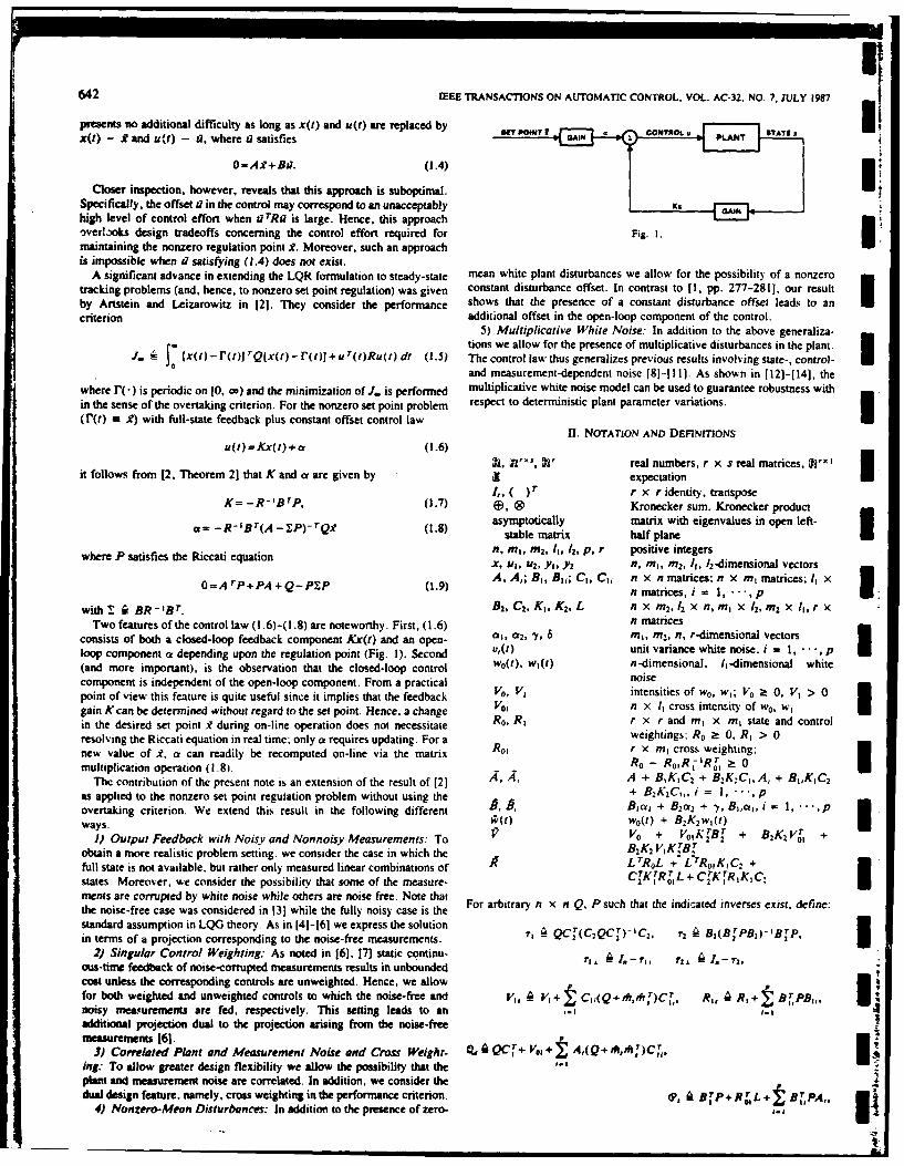
642 IEEE TRANSACTIONS ON AUTOMATIC CONTROL. VOL. AC-32. NO. 7, JULY 1987

presents no additional difficulty as long as x(t) and u(t) are replaced by "x(t) - it and u(t) - a, where a satisfies

0=A.9+B1. (1.4)

Closer inspection, however, reveals that this approach is suboptimal.Specifically, the offset d in the control may correspond to an unacceptably Kxhigh level of control effort when a rRa is large. Hence, this approachoverl3oks design tradeoffs concerning the control effort required for Fig. 1.maintaining the nonzero regulation point .9. Moreover, such an approachis impossible when &7 satisfying (1.4) does not exist.

A significant advance in extending the LQR formulation to steady-state mean white plant disturbances we allow for the possibility of a nonzerotracking problems (and, hence, to nonzero set point regulation) was given constant disturbance offset. In contrast to [I, pp. 277-281], our resultby Artstein and Leizarowitz in [21. They consider the performance shows that the presence of a constant disturbance offset leads to ancriterion additional offset in the open-loop component of the control.

5) Multiplicative White Noise: In addition to the above generaliza-tions we allow for the presence of multiplicative disturbances in the plant. l

x(t) - 12(t)] rQlx(t) - 1(t)] + u r(t)Ru(t) dt (1.5) The control law thus generalizes previous results involving state-, control-and measurement-dependent noise 81-1111. As shown in [12J-[141, the

where r(.) is periodic on [0, 0o) and the minimization of J. is performed multiplicative white noise model can be used to guarantee robustness within the sense of the overtaking criterion. For the nonzero set point problem respect to deterministic plant parameter variations. 3(r(t) - .?) with full-state feedback plus constant offset control law

11. NOTATION AND DEFINMONSu(t)=Kx(t)+ a (1.6)

R, 1'S, 32' real numbers, r x s real matrices, 7'1 Iit follows from [2, Theorem 21 that K and a are given by K expectation

,, ( )T rr x r identity, transposeK= -R-IB TP, (1.7) , ® Kronecker sum. Kronecker product

asymptotically matrix with eigenvalues in open left-a= - R- Br(A -P)- rQ? (.8) stable matrix half plane

where P satisfies the Riccati equation n, MI, M2, 11, 12, p, r positive integersX. ul, U2, y,, Yz n, ml, m2 , 11, /2-dimensional vectorsA, A,; BI, Bli; C,, Ci n x n matrices, n x ml matrices; 11 X 3

O=A rp+PA ++Q-PZP (1.9) n matrices, i = 1, - , p

with" Z BR-IBT. B2, C2, KI, K2 , L n x m 2,1 2 X n~m, X 12, m2 X 11, r XTwo features of the control law (1 .6)-(1.8) are noteworthy. First, (1.6) n matrices

consists of both a closed-loop feedback component Kx(t) and an open- al, af2, ", m in, m2, n. r-dimensional vectorsloop component a depending upon the regulation point (Fig. I). Second v,(t) unit variance white noise, i = 1, • ., p I(and more important), is the observation that the closed-loop control wo(t), wI) n-dimensional, l,-dimensional whitecomponent is independent of the open-loop component. From a practical noisepoint of view this feature is quite useful since it implies that the feedback Vo, V, intensities of wo, wl; V0 a 0, V > 0gain Kcan be determined without regard to the set point. Hence. a change Vol n x 11 cross intensity of w0 , wlin the desired set point 9 during on-line operation does not necessitate R0 , R, r x r and ml x ml state and controlresolving the Riccati equation in real time; only a requires updating. For a weightings: R0 -- 0, R, > 0new value of .i, a can readily be recomputed on-line via the matrix Rol r x m, cross weighting;

multiplication operation (.8). R+ - Ro)R, Roi - 01The contribution of the present note is an extension of the result of [2] 4, A A + BK 1 C2 + B2 K2 C, A, + BI,KC 2

as applied to the nonzero set point regulation problem without using the + BK 2C,,, i = 1 , - • , povertaking criterion. We extend this result in the following different A. 17 Blal + B2a 2 + f, Bl,, i , ',p-ways. 17(I) Wo(t) + B2K2w,(t)

1) Output Feedback with Noisy and Nonnoisy Measurements: To " Vo + VoKBr + B 2 Vr +obtain a more realistic problem setting. we consider the case in which the B2 K2 VKTBTfull state is not available, but rather only measured linear combinations of L TRL + ' L:TRo KC +

states. Moreover, we consider the possibility that some of the measure- C2 KR 0 1L + C KrR IAK I CI

ments are corrupted by white noise while others are noise free. Note thatthe noise-free case was considered in 131 while the fully noisy case is the For arbitrar n x n Q, P such that the indi'ated inverses exist, define:standard assumption in LQG theory As in (4]-[61 we express the solutionin terms of a projection corresponding to the noise-free measurements. ' - QC 2'(C 2QC 2)-C 2 , r , B,(BrPB,)-'Brp,

2) Singular Control Weighting: As noted in [6], [7] static continu-

ous-time feedback of noise-corrupted measurements results in unbounded t * 1. -cost unless the corresponding controls are unweighted. Hence, we allow 1lfor both weighted and unweighted controls to which the noise-free and V1, 4 V,+ C,(Q+ I )C, RI, , R ,+ BrpBI, 1noisy mew.urements are fed, respectively. This setting leads to an -I ,.additional projection dual to the projection arising from the noise-freemeasurements 161.

3) Correlated Plant and Measurement Noise and Cross Weight. . QC r+ vo + A,(Q+ rh,A 7)C rIng., To allow greater design flexibility we allow the possibility that theplant and measurement noise are correlated. In addition, we consider thedual design feature, namely, cross weighting in the performance criterion. t?, ABrp+RrL+ B

4) Nonzero-Mean Disturbances: In addition to the presence of zero- 0 Bp

it

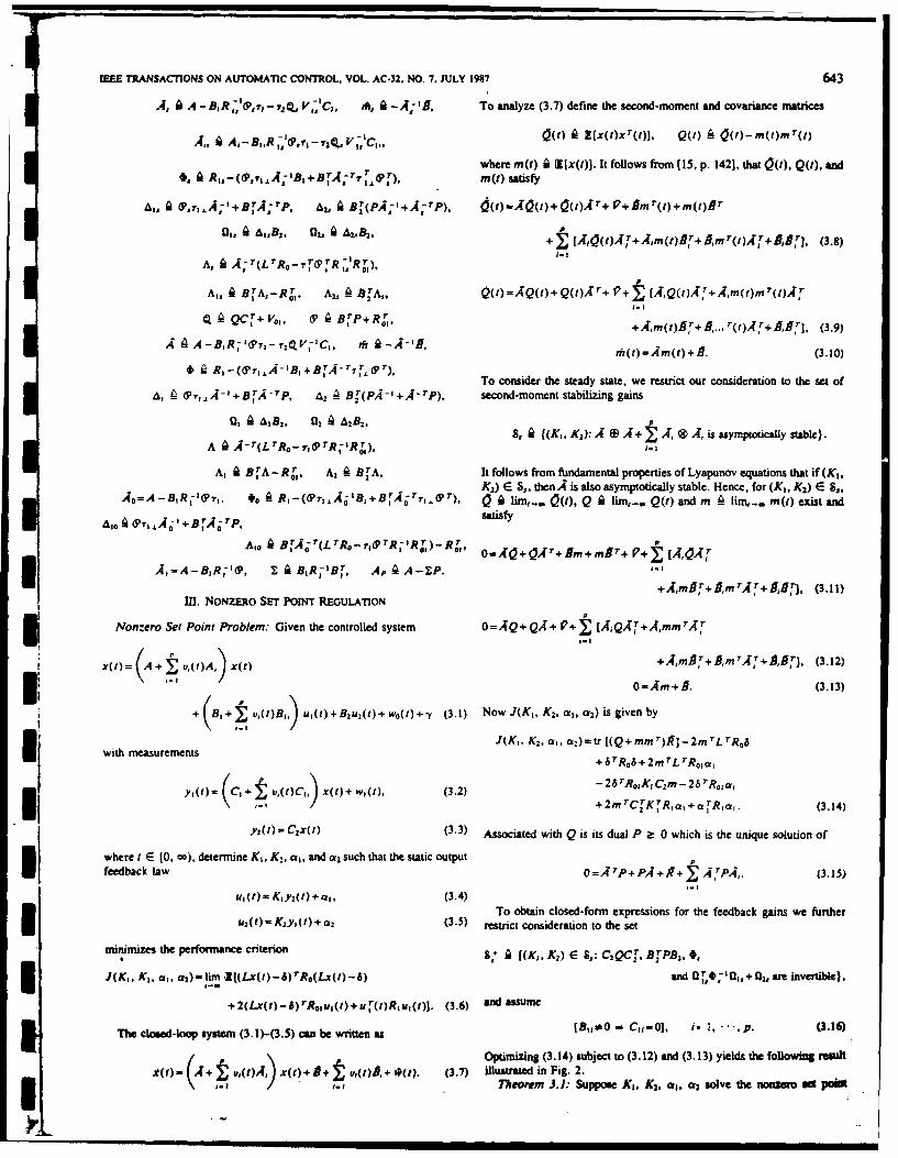
UEEE TRANSACTIONS ON AUTOMATIC CONTROL. VOL. AC-32. NO. 7. JULY 1987 643

A, A A - , R ,7, -r., V ,'C,, ph, a -A;' , To analyze (3.7) define the second-moment and covariance matrices

A,, A A4-B,,R Is '1,-r1-72CL V -

Is 'Cl . Q(t) a l.x(twx(t)]. Q(t) -A a (t-mmtmr(t)

where m(t) A i[x(t)]. It follows from [15. p. 142], that Q(t), Q(t). and1 ST), m(t) satisfy

a,, 9 (P,7,,,+BrA;r, , Br(PA;2 +,+;rP), d 0 (+ (t)t+ p+jmr+m(+m(t) r

II I01. t A1182. 02, 'l A,2.182 +J; [/[,0t)/,+,Am(t)Jr,+fm r(t) r+AffB,, (3.8)

I T Is-tA, - A;T(L TRo- rT(R7,IR,).

A,, A ETA,-Ro. A . A O'rA,, Q(t)='AQ(t)+ Q(t)A)+ ++,m(r)mrOt)A ,I-I

-QC Tr+Vo, d1 BTP+RT. +Ajm()AT.+ ,...r(t)AT+I,TI, (3.9)

A 19 A-BR-'(i,-2.F'C 1, h 9-A-9 . m(t)=Am(t)+f. (3.10)

Q (r 1 To consider the steady state, we restrict our consideration to the set of

A, ~_ t)T ,~1 +~-+ Ar, -p A2 _ Br(PA-+A-Tp). second-moment stabilizing gains

0, al82, 02 AA2B, P8, 9 {(,, K2):A D ,A+ A, 9 A, is asymptotically stable).

A ,-T(LrRo-_r R-IRT), .1

A, ; BrA-R r A, - B A. It follows from fundamental properties of Lyapunov equations that if (KI,2K2) E 9,, then A is also asymptotically stable. Hence, for (K I , K2) E 9,A,=:A -B,R IT7,. f, A R,-(?r ,,Ao'Bg+BTro r t lim,-. Q(t), Q A Kr ., Q(t) and m A lim,., mt) exist and

ago A 6l71, A -I+B rA -TP, satisfy

A,0 e . of;T(, TRo-,TR RT)-RT, O,(A+oAr+Bm+mr + p+,(AAr

A,=A- RI', A B, RT'BT, A , AA-ZP. i

+,,,m1,T +A m /[r +fff, . (3.11)M. NONZERO SET POINT REGULATION

Nonzero Set Point Problem: Given the controlled system 0=AQ+QA+ 17+1 [A,QA1T+Amm TAr

x(t)=(A+ v,(t)A, x(t) +A,mAr+,mrAT+ ,fri , (3.12)

"A 0=/m+A. (3.13)

+(B,+tu,(t)B,) u1()+B 2 u2 (t)+wo(t)+' (3.1) NowJ(K1 , K2,a,0,2) isgivenby

J(K,. K2, al, C12) =tr H(Q+MMT)A1 2mL T Robwith measurements C TRo6 + 2 m TL T Roaof

-26 TRoK1Cim -26 TRy l( f ) = C J + . t ) W C l, X ( ) + w , ( t ), (3 .2 ) + m c ~ R m a R a .( .4

+2m TC K R. , + aTR, a,. (3.14)

y?(t) = Czx(t) (3.3) Associated with Q is its dual P a 0 which is the unique solution of

where I E 10, D), determine KI, K., a,, and c 2 such that the static outputfeedback law O=A P+PA, +A+z ATPA,. (3.15)

u,(t)rKiy2 (t)+cr,, (3.4)

To obtain closed-form expressions for the feedback gains we furtheru(t)=K2y,(1)+a 2 (3.5) restrict consideration to the set

mmnnzes the pfomnce citerion (.X)E5,CQCBP ,*a2 )lim K2) E &,: C2QCo(LBrPt2-6

J(K,, K2 . at,,)-lim 3t(Lx(t)- &)rRo(Lx(t)-6) and O r Q,",0,, + 02, are invertible).

+2(Lx(t) -8)r R0, u,(t)+ur(,)R,U,(t)]. (3.6) and assume

The closed-loop system (3.1)-(3.5) can be written as (B,00 - Cu-O], i. 2, "''.p. (3.16)

Optimizing (3.14) subject to (3.12) and (3.13) yields the following remnt

. A+ v,(t)A, x(t)+O+ u,4V(e+ *(). (3.7) illustrated in Fig. 2.Theorem 3.1: Suppose KI, K3, *I, a, solve the nonzermo sat poiti

644 IEEE TRANSACTIONS ON AUTOMATIC CONTROL. VOL. AC-32. NO. 7. JULY W97

COWTA~ffIV. SPECIALIZATIONS OF THEOREM 3.1

To draw connections with the previous literature, a series of specializa-tions of Theorem 3.1 is now given. We begin by deleting all multiplicative

GAN Ck~mwhite noise terms, i.e.,

.WE 9UA,, B,,, Clic0. i= I, ,p. (4.1)

a, WUJO4 U NT In this case the stabilizing set S.can be characterized by

"MV YJ 8= {(K,, K2): A is asymptotically stable),

KIP2 4 161moly Y2and, furthermore, 8 becomes

Fg. 2. j (X,, K,) E S: C,QCr2 , BT'PB,

problem with (KI, K2) E 81 Then there exist n x n Q, P ;t 0 such that I ad04'fv-2reivertible).

Corollary 4.!1: Assume (4. 1) is satisfied and suppose K,, K2, a,, a2zK,=-R_'6P5QCj(C 2QCfj)-', (3.17) solve the nonzero set point problem with (K,, K2) E 8 *. Then there exist

n x n Q, P a 0Osuch that

14 (BP 2 -'rQ.,~,(3.18) K,= -Ri tQC1(C 2QC1)'I, (4.2)

1= s(Q.9 &.y- j,(3.19) K2= (B 1PB2) -IB fPQV1- 1 (4.3)

and such that Q and P satisfy' and such that Q and P satisfy

0 (A -B,R -16,r)Q +Q(A - B,R -'tP.,r,)T+ Vo 0= (A -B, R I6'rj)Q +Q(A - BB 1 )7-1 r,+ Vo

_BV=O, C,=0.(ZIqT (4.8)-ICIr2 ~ V,, 1 C,)(PP( - 1&'C2+R V U )+

Thishff corsod to theifs6 setn +0sdr~di 3. It folow fro th proof IJAIS ~~o s .Indth ore 3 4.1 ) htte assump tion tha al0ladonto ar e 0. igan d and

Outi o Poo: s i 16]th rsuti s obaie by, forming the mesreet ar n ois free, ani4arei.,tbl

Lagrangian whil aconi (3.2 an (3.13) CYolr 4.2: Asum (4. and (48 are saise an supos (48

andis cosot theozr setint robem ith A3. Et folow Then therois

+P ofH TheoremXTAmA) 3. = 1 -tattheasumpio(BC2=0Cead t-, (4.9)dC,=

whr + (A 0 and V E sC, TPA Setn 72/Q, V 0 sCj andepod usin thetin second- Henc 84 an 8. +) ar4.10)veb

moment.22 stbiot assmpio itC folow thatotcal staIbithutlos)o

with~~~~~, repc to E, 8,, C,, QC, rn an to zero andsovinrfriteain..TO utsistte o rea in caring out1 the destis w otied tha fi g iven by2ABR'~ 1 Q QA B,,c?)+V, (

and Wo seciaeiozer fute onth fulblae feedak caseihe., thrxs2-LK2 l o- . t

r J(,, K,,6-~KRa al n 2 , (4.Q13):0 uc ta

Remark3.I:+ Dcuefh Presencof (3.12))viaad~n andhncer + Kad. = 0. - o8ad~bm I6QTCCT-1(49(see Xhe de2tio of0 and 1 R.Sting 328 =0ad sn the lsdlopcmo en -ft the- -A ).(.0moment sblaw y assumption0 cant folldsge tndependentlyfthe loen of,~(, +, saypoiclysal)gopcoentr. eiaio now howb etinence partrecoverivtwhe the dsuhta QadPaif

Tultipsicaivehnoreederm caren autbendtisw etat8 X , is invebrt A BBI- QA IBl).r Io 4.1

IEEE TRANSACTIONS ON AUTOMATIC CONTROL, VOL. AC-32. NO. 7, JULY 1"17 645

Corollary 4.3: Assume (4.1). (4.8), and (4.13) are satisfied and Analysis of Time-Varying Scaled Systems Via Generalsuppose K, and a, solve the nonzero set point problem with K, E S" OrhgnlPoyo ilThen there exist n x ni Q, P z: 0 such that Otooa oyo il

Kim -R'i 1, (4.14) TSU TIAN LEE AND) MI FONG CHANG

of 0R16 Abstract-Geseral orthogonal polynomials are introduced to analyzeand approximate the solution of a class of scaled systemss. Using the

(4.15) operational matrix of Integration, together with the operational matrix of

and such that Q and P satisfy linear transformation, the dynamical equation of a wcalled system Isreduced to a set of simultaneous linear algebraic equations. The

0=(A -BIR) Idl)Q+ Q(A -BIRJ -16) T+ V0, (4.16) coefficient vectors of the general orthogonal polynomials can be dete-mined recursively by the derived algorithm. An Illustrative example Is

0=A rp+ pA + R0 - (p TR, 6, (4.17) given to demonstrate The validity and applicability of Mhe orthogonalpolynomial approximations.

Finally, setting 1. INTRODUCTION

-= 0. Rol = 0, L =1. (41) An investigation of the dynamics of an overhead current collectionwe otainthe esul of 2).mechanism for an electric locomotive by Ockendon and Taylor (121

Corollary 4.4: Assume (4.1), (4.8). (4.13). and (4. 18) are satisfied revealed that under certain conditions, the dynamics of the systems isand uppse , ad a sove he onzeo st pintprolemwit KE 9 characterized by a differential equation containing terms with a scaled

Then there exists n x n P a 0 such that agmn ftefr

K,= -R-'B~p, (4.19) X(t)=AX(Xt)+BXQl)

oti -_R - irA - R,6 (4.20) X(0)-X 0

and such that P satisfies where XOIJ) and XQt) are n-vectors and A and B ame n x n matrices andthe constantO0 < X < 1. This type of differential equation also plays an

0=A rP+PA +Ro-PIP. (4.21) important role in several chemical processes [31, [13]. This equation wasfirst studied by Fox ef al. (11] with the introduction of a finite differencemethod forO0 < X < 1.Recently, the solution of such ascaled system has

REFERENCES been obtained by several different orthogonal functions, such as block-(11 K. Kwakernaask and R. Sivan, Linear Optimal Control Systems. New York: pulse functions (141, (21, [31, Walsh functions 1]1, delayed unit step

Wiley. 1972 functions [4], Laguerre polynomials [5], Chebyshev polynomials [6], M'7,(21 Z. Amasin and A. Leiwaowitz. "Tracking periodic sunas with the overtaking and Legender polynomials [ 15]. The common approach of these methods

criterion." IEEE Trans. Automat. Cant,.. vol. AC-30. pp. 1123-1126. 1985. is the use of the operational matrix of integration together with the13) W. S. Levine and M. Ailsans. "On the determination of the opitimal constant operational matrix of scaling to reduce the differential equation to a set ofoutput feedback gains for linear multivariable systetrs." IEEE Trans. Automat,. ieragbaceutos hc s oesial o optrporm

Comm,. vol. AC-1S. pp. 44-48. 1970. lna leri qainwihi oesial o optrporm141 J. Medanic. "On stabilization and optimization by output feedback." in prc uing.

12th Asilomar Conf! Circ., Syst. Comp.. Pacific Grove, CA. Nov. 1978, pp. In this note we will employ the operational matrix of integration and412-416.

15) J. V. Medanic. "Asymptotic properties of dynamic controllers designed by product operational matrix of the general orthogonal polynomials,projective controls," in Proc. 24th IEEE Con. Decision Contr.. For together with thc operational matrix of linear transformation, which willLauderdale. FL. Dec. 1985. be derived later, to obtain the solution of the scaled system. The

161 D. S Bernstein, -The optimal projection equations for static and dynamic output operational matrix of linear transformation is derived based on thefeedback The singular cast." IEEE Trans. Automat. Contr.. to be published following properties. namely, the pure recurrence relation

(71 S. Basuthakssr and C. H. Knapp. "Optimal constant controllers for stochasticlinear systems." IEEE Trans. Automat. Cont, vol. AC-2O. pp. 664-666, , 1 z=ozb)~()c~iz 11975. 0 ~)=(z+b),z * z 1

181 W. M Wonham., "Optimal stationary control of a linear system with state-dependent noise." SIAMI. Contr.. vol 5. pp. 4W6500, 1967. with

(91 D Klemnman, "Optimal stationary control of linear systems with control-dependent noise." IEEE Trans. Automat. Contr., vol. AC-14, pp. 673-677. 0o(z) = I; 0iU) = aoz+ be1969.

1101 P. McLane, "Optimal stochastie control of linear systems with state and control- and the differential recurrence relationdependent disturbances."- IEEE Trans. Automat. Contr.. vol. AC- 16, pp. 793-798, 1971.

Ill] J. Bismut. "Linbear-quadratic optimail stochastic control with random cofi 0,(z) = Aj,. (z) +B,,z)+-Ci, W( (2)dents." SIAM J. Contf, vol. 14. pp. 419-444. 1976,

1121 D S. Bernstein and D. C. Hyland. "The optimal projectionimaximum entropy where recurrence coefficients a,, b,, c, and differential recurrenceapproach to designing low-order. robust controllers for flexible structures." in coefficients A,, B,, and C,, are specified by the particular orthogonalProc. 24th IEEE Conf. De'ision Contr.. Fot Lauderdale. FL. Dec. 1985, pp. polynomials under consideration and some are listed in (91. The aim of745-752.

1131 D. S. Bernstein anld S. W. Greeley, "Robust controller synithesis using th this paper is twofold: 1) to derive an operational matrix of iearmaximum entropy design equations," IEEE Trans. Automat. Contr.. vol. AC- transformation for general orthogonal polynomials so that the scaled3J1. pp. 362-364, 1986.

I 14] -. Robust output-feedback stabilization: Deterministic and stochastic per-spectives." in Proc. Amer. Comtm Coot!.. Seale. WA. June IM1, pp. 1818- Manuscript received December 6. 1985. revised April 14, 1986 and September 9.1321, 1966.

(151 L. Arnold. Stochastic D(fferendul Equaitions: Tinot)' and Applicatioln. T. T. Lee is witds the Department o( Electrical Engineerng. University of Kentucky.New YWork: Wiley, 1974. Lexington. KY 40506-4W.

(161 D. C. Hyland and D. S. Bernstein, "Thme optial projection equations for flaad- Y. F. Chiang is with the Institute of Electronics, National Chsao Tung University.adoe dynamic compensation," IEE Train. Asmtamet. Contr.. *Vol. AC-29. pp. Taiwan. Republic of China.1034- 10"9, 1914. IME Log Number 8714806.

00l1-9286&S7/0700.0645S01 .00 0 1987 IEEE

I

INT. J. CONTROL, 1988, VOL. 47, NO. 2, 529-536

I Optimal output feedback for non-zero set point regulation:the discrete-time case

WASSIM M. HADDADt and DENNIS S. BERNSTEIN +

Optimal discrete-time static output feedback is considered for a non-zero setpoint problem with non-zero mean disturbances. The optimal control law consistsof a closed-loop component for feeding back the measurements and a constantopen-loop component which accounts for the non-zero set point and non-zerodisturbance mean. An additional feature is the presence of state-, control- andmeasurement-dependent white noise. It is shown that in the absence of multipli-cative disturbances, the closed-loop controller can be designed independently of theopen-loop control.

INotation and definitions

R, R' 3, R', E real numbers, r x s real matrices, R'', expectation.,, ( n x n identity, transpose

Kronecker producttr Z trace of square matrix Z

asymptoticallystable matrix matrix with eigenvalues in the open unit disk

n, m, 1, p positive integersx n-dimensional vector

u, y m-, I-dimensional vectorsA, A,; B, B1; C, Ci n x n matrices, n x m matrices, I x n matrices, i= 1. p

L, K r x n matrix, m x l matrix5, y, a r-, n-, m-dimensional vectors

k discrete-time index 1, 2, ...vi(k) unit variance white noise, i = I ... , p

w,(k), w2(k) n-dimensional, -dimensional white noise processesV,, V n x n covariance of w1, I x I covariance of w2 ; V > 0, V2 > 0

V12 n x I cross-covariance of w1, W 2

R, R2 r x r and m x m state and control weightings; R, > 0, R 2 >10R12 r x m cross weighting; R, - R12 R-IR'2 > 0

A,A A+BKC, A1+BjKC+BKC,i=. pA 1.-J

I , Bi+

S= w, + BKw2 + B1Kw2

Received 9 March 1987.t Department of Mechanical Engineering, Florida Institute of Technology, Melbourne, FL

32901, U.S.A.: Harris Corporation, Government Aerospace Systems Division, MS 22/4848, Melbourne,

FL 32902, U.S.A.

II

I I I

I

530 W. M. Haddad and D. S. Bernstein

V, V+ V,.K TBT+ BKV 12 + BKV2KT B T + BjKV2K TBT

RL TRL+L TR 12KC+ CTKT R 2 L+ CTKT R2KC

+ CTKTR 2 KCj IFor arbitrary m e R" and Q, P c Rn x define:

R2.3AR 2 +B T PB+ BjTPBj, V2, - V2 +CQC T + T C(Q+mmnr)CT

R 2. A R 2 + BT PB, V -V 2 + CQCT Ip p

P, ABT PA+RL2t+ B'PA,, Q, AQC +V 12 + Aj(Q+mm T )C'Po -BTA ArPA + R Q AQC T + V 2

PsART2 + BPA ,+A v 12 + A,(Q4- mT)CTR1 l Qs i=1 + AI

1. IntroductionThe quadratic performance criterion

NJ= r(k) R, x(k) +u(k)R2uk (1)

expresses the desire to minimize deviations of the state x(k) of the system

x(k + I) = Ax(k) + Bu(k) + wok) (2)

from the regulation point x = 0. As is well known (Kwakernaak and Sivan, 1972, Ipp. 504-509), the non-zero set point criterion

NJ, [x(k) - ]rRI[x(k) - ] + uT(k)R,u(k) (3)

k=OI

presents no additional difficulty so long as x(k) and u(k) are replaced by x(k) - . andu(k) - il, where a satisfies

x = A-i + Bui (4)

Closer inspection, however, reveals that this approach is suboptimal. Specifically,the offset ii in the control may correspond to an unacceptably high level of controleffort when aT R2 i is large. Hence (3) overlooks design tradeoffs concerning thecontrol effort required for maintaining the non-zero regulation point .i Moreover,such an approach is impossible when ii satisfying (4) does not exist.

A significant advance in extending the full-state-feedback LQR formulation to Isteady-state periodic tracking problems (and hence to the special case of non-zeroset point regulation) was given by Artstein and Leizarowitz (1985). Bernstein andHaddad (1987 b) generalize the results of Artstein and Leizarowitz (1985) for the non-zero set point regulation problem to include noisy and non-noisy measurements, Iweighted and unweighted controls, correlated plant/measurement noise, cross weight-ing, non-zero mean disturbances, and state-, control- and measurement-dependentmultiplicative white noise. They consider the steady-state performance criterion I

J = lim E(Lx(t) - )TRI(Lx(t) -)+2(Lx(t)-_)R12ut+UT( t) R2(0)1 (5)

II

Non-zero set point regulation 531

3 where 6 is the non-zero regulation point. For full-state feedback with R, 2 = 0 and

L= identity, Artstein and Leizarowitz (1985) show that for a constant offset control law

Su(t) =Kxt) +x (6)

K and at are given bv

K =-R2BTP (7)

a = -R- B T (A -P-TR,6 (8)

where P satisfies the Riccati equation

0= ATp+ PA + R -P.P

with

3I

Two features of the control law (6)-(8) are noteworthy. First, (6) consists of both aclosed-loop feedback component Kx(t) and an open-loop component oc dependingupon the regulation point 6. And, second (and more important), is the observationthat the closed-loop control component is independent of the open-loop component.From a practical point of view this feature is quite useful since it implies that thefeedback gain K can be determined without regard to the set point. Hence a change inthe desired set point 6 during on-line operation does not necessitate re-solving theRiccati equation in real time; only a requires updating. For a new value of 6, ot canreadily be recomputed on-line via the matrix multiplication operation (8). In thepresence of multiplicative disturbances, however, the independence of the closed-loopcomponent from the open-loop component is lost.

The purpose of the present paper is to provide a self-contained derivation of theoptimality conditions for the non-zero set point problem in the discrete-time case. Toobtain a realistic problem setting, we consider the case in which the full state is notavailable, but rather only noise-corrupted measurements of linear combinations ofstates For greater design flexibility, we also allow the possibility for correlated plantand measurement noise. In addition, we consider the dual design feature, namely,cross weighting in the performance criterion. The presence of a non-zero constantplant disturbance in conjunction with zero-mean white plant disturbances, i.e. a non-zero mean disturbance, is also considered. Our results show that the presence of anon-zero constant disturbance component leads to an additional offset in the open-loop component of the control. Finally, in addition to the above generalizations weallow for the presence of multiplicative disturbances in the plant. The control law thusgeneralizes previous results involving state-, control- and measurement-dependentnoise (Bernstein and Haddad 1987). As shown in Bernstein and Greeley (1986) andHaddad (1987), the multiplicative white noise model can be used for robustness withrespect to plant parameter variations.

2. Non-zero set point regulation

2.1. Non-zero set point problemGiven the nth-order controlled system

I x(k+ 1) = (A + , vi(k)Ai)x(k) + (B+ i vi(k)Bi) u(k) + w,(k) + 7 (9)

II

II

532 W. M. Haddad and D. S. Bernstein

with measurements UXk C+ Vi(k)C x(k) +w2(k) (0

where k = 1, 2,..., determine K and a such that the static output feedback controller

u(k) = Ky(k)+o (1l) 3minimizes the steady-state performance criterion

J(K, e)4 Alim E[(Lx(k) - 6)'R,(Lx(k) - 6) + 2(Lx(k) - 6)T R12u(k) + uT (k)Rzu(k)]

(12)

Using the notation of § I the closed-loop system (9)-(11) can be written as

To analyse (13) define the second-moment and covariance matrices

,.(k)A E[x(k)xT(k)], Q(k) 4 4,(k) - m(k)mT (k)

where m(k) A E[x(k)]. It follows from (13) that Q(k), Q(k) and m(k) satisfy

(7(k + 1) = AQ(k)AT + Am(k)f T + BmT(k) A T + B&T

+ = [Aj(k),?T+ Am(k)A + Am(k)T+ fffT]+ F/ (14)

Q(k + 1) = AQ(k).AT + [AQ(k)A r + Ajm(k)mT (k).4rYi= 1l

+Ri mT(k)ART + Ajm(k)/] + V (15)

m(k + 1) = Am(k) + Bf (16)

To consider the steady state, we restrict our consideration to the set of closed-loopsecond-moment stabilizing gains

S,4 {K:®DA+ Ai .®A, is asymptotically stable}

It follows from fundamental properties of Lyapunov equations that if K C S,, thenA is also asymptotically stable. Hence, for K c S,, 19 lim 0(k), Q A lim Q(k) and

m A lim rn(k) exist and satisfy

-AOT + A T -- mT- TT+ AgT I

+ [A + RBMi MT T + Ai fm + A1 1T,] + V/ (17)

Q= AQAT + [,iQAT+ AZmmT. + BimT4 T + AmBT + Br] + V, (18)

m=A 9 (19)

Note that since A is asymptotically stable, the inverse in (19) exists. For K - S,, it now

II

Non-zero set point regulation 533

i follows that J(K, a) is given by

J(K, a) = tr [(Q + mmT)k] + tr [KT R2 KV2 ] + 6T R,6 - 2mT LT R, a

+ 2mTrLT R2 ,- 26t 2 2KCm - 2TR, 2 a + 2mTCTKTR 2 2 + OTrR 22 (20)

Associated with Q is its dual P > 0 which is the unique solution of

P = V T P,+ I. 1 rpj,+ (21)iz I

To obtain closed-form expressions for the feedback gain K, we further restrictconsideration to the set

S+ A {K E S,: R 2, > 0, V, > 0 and T, is invertible}where

IPS A BTrA-TLTR, LA B + BTA - T LTR12 (I + KCA -'B)

+ (I, + KCA- B)TR1 2LA 'B + (in + KCA- B)TR 2 (I, + KCA- 'B)

I + [BTA-TAIPAiA-'B+ BPiA-'B+BTA-TATPBi1=1

+ BTPBj + BTA-TCYKTR2KCiA-'B]3 Furthermore, we assume that

[B 06 --:Cj=0], i=l,...,p (22)i.e. for each i e (1.p}, Bi and Ci are not both non-zero. Essentially, (22) expressesthe condition that the control-dependent and measurement-dependent disturbancesare independent. There are no constraints, however, on correlation with the state-dependent noise. For the statement of the main theorem define

A, - BTA-TLT(R, L+ Rl 2 KC)A-' + (i,. + KCA- IB)T(RI 2 L + R 2KC)A-'

+ ([AA-'B+B]TPiA-' + BTA-TCTKTR 2 KCiA-)

SBTA-L T RL+ RT 2L+ B A CKT R1ZL

* Theorem 2.1Suppose K and x solve the non-zero set point problem with K e S,'. Then there

exist n x n Q, P > 0 such that

K = -R-l(BT PAQC + P" QC + BTPQ 1 ) V2;I (23)2= _-,-- '[A,-,,+ 0 6] (24)

3 and such that Q and P satisfy

Q= AQAT + VI + [(.4+ B1KC)Q(Aj + BjKC)T + BjKV 2 K T BT + AimmTA

+ ginlT'4 + ,iMfT +

+(Q, + BK V2.) V2 '(Q. + BK V23)T Q 3V 3 Q (25)

P= 4 T PA+R, + [(Ai+BKC,)TP(A,+BKCj)+CKTR2 KC,

+ (P, + R2,1KC)TR2,'(P,+ R2,KC) - PTR 2,SP,] (26)II

534- W. M. Haddad and D. S. Bernstein

Proof

The derivation of the necessary conditions is a straightforward application of theLagrange multiplier technique. To optimize (20) over S+ subject to the constraints(18) and (19), form the lagrangian

(K, a, Q, P, m) A tr i.oJ(K, ct) + (,QAr + . [AQiT + ,4immT,4 + BimT,

+~~A AT 9] + r/Qp+ ;.T(,Ir +, I Mr)]

where the Lagrange multipliers ,0 > 0, . e R" and P c R"'" are not all zero. Setting8L/LQ = 0 and using the second-moment stability assumption it follows that , = Iwithout loss of generality. Thus the stationarity conditions are given by

A1" = ATP,+ 4 TP,4iA+R-P =0 (27) 1aQ i=1

OL= AQ + (A Q4 +..4i....... + A~m T4 + A iM flI + qiffi

+ I--Q=0 (28)

dL 4 m+-m=o (29) I2L = R2,K V2 , + R T2 QCT + BT PAQCT 3

+ [BiPAQC+BTpAi(Q+mm )CT]+BTPVi2 =0 (30)

J = [B:TPAim + BLYPBiKC + B:TPBit] + -BT + R{ 2 Lm

-R, 2 6+R 2 KCm+R 2ct=0 (31)

am 2

CT KT RT26 + CT KT R2x=O (32)

A=2A-T(RAm+ [AiyPAi+ A1PAYm]-LTR,6+ LTR, 2 ,7

-CT KT R126+ CKT R 2 3:) (33)

Using the definitions for Q3, and P,1 along with (33), we obtain (23) and (24).Substituting the expressions for the optimal gains into (27) and (28) yields (25) and(26). 3Remark I

Because of the presence of 6 in (25) via m in both Q,1 and V2, and in (25) via B(in m) and #,. the closed-loop component of the control law (23) cannot be

Ii

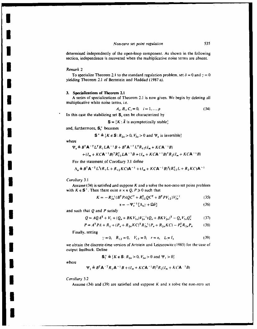
Non-zero set point regulation 535

I determined independently of the open-loop component. As shown in the followingsection, independence is recovered when the multiplicative noise terms are absent.

I Remark 2

To specialize Theorem 2.1 to the standard regulation problem, set 6 = 0 and ,. = 0yielding Theorem 2.1 of Bernstein and Haddad ( 1987 a).

3. Specializations of Theorem 2.1A series of specializations of Theorem 2.1 is now given. We begin by deleting all

multiplicative white noise terms, i.e.

Ai, Bi, Ci=0, i=l..., p (34)3 In this case the stabilizing set S, can be characterized by

S = {K:, is asymptotically stablel

and, furthermore, S' becomes

S' eK S:R2a >O, V2 > 0 and Ta is invertible}where

T.'a A BTA -T LTR, LA- 1 B + BTA-rLTR,2(I. + KCA- 'B)

+(I, + KCA- B)TR1 2 LA- 'B +(I,, + KCA- B)TR,(I, + KCA- B)

For the statement of Corollary 3.1 define

A. A BT A -T LT(R, L + R12 KC)A- + (Im + KCA-B)T(RT, L + R2 KC)A- I

Corollary 3.1Assume (34) is satisfied and suppose K and 2 solve the non-zero set point problem

with K e S'. Then there exist n x n Q, P > 0 such that

3 K= -R-(BT pAQCT + R tQCTR +B PV2 )V2i i (35)

o( = - 'P- ' [A.,' + 06] (36)

and such that Q and P satisfyI Q= AQA+ V +(Qa+ BKV2a)V-'(Qa + BKV 2a)-QV Qa (37)

P= ATPA + R, +(P + R 2 KC)Rl(P + R 2 KC) T pR 2 , P (38)

3 Finally, setting'=0, R1 2 =0, V12=0, r=n, L=I. (39)

we obtain the discrete-time version of Artstein and Leizarowitz (1985) for the'case ofoutput feedback. Define

S+ {KeS:R2 a>O, V2a>O and T, >0where

w h , A BtA-tR A - 'B + (im + KCA- B)TR 2(Im + KCA-'B)

3 Corollary 3.2

Assume (34) and (39) are satisfied and suppose K and x solve the non-zero set

II

II

536 Non-zero set point regulation

point problem with K e S'. Then there exist n x n Q, P > 0 such that

K = -R' B T PAQC T V27, (40)~= _P- tBTA-TR1 5 (41)

and such that Q and P satisfy

Q=AQA T + V, + (AQCT + BK V2a) V l(AQCT + BK V2 )T

- AQCT V2aCQA T (42)

P = ATPA + R, + (BTPA + R 2aKC)TR2al(BTpA + R2 aKC)

- A T PBR2UB T PA (43)

4. Directions for further researchThe extension to fixed-order dynamic compensation for non-zero set point

regulation appears possible using the approach of Hyland and Bernstein (1984)and Haddad (1987). A generalization of Theorem 2.1 to design periodic trackingcontrollers (either static or dynamic) via the parameter optimization approach isbeing developed.

ACKNOWLEDGMENT

Dr Bernstein was supported in part by the Air Office of Scientific Research under

contract F49620-86-C-0002.

REFERENCES

ARTSTEIN, Z., and LEIZAROWITZ, A., 1985, I.E.E.E. Trans. aurora. Control. 30, 1123.BERNSTEIN, D. S., and GREELEY. S. W., 1986, I.E.E.E. Trans. autom. Control, 31, 362.BERNSTEIN, D. S., and HADDAD, W. M., 1987 a, Int. J. Control, 46, 65: 1987 b, I.E.E.E. Trans.

aurom. Control, 32, 641.HADDAD, W. M., 1987, Robust optimal projection control-system synthesis. Ph.D. dissertation.

Department of Mechanical Engineering. Florida Institute of Technology. Melbourne.FL.I

HYLAND, D. C., and BERNSTEIN, D. S., 1984, I.E.E.E. Trans. autom. Control, 29, 1034.KWAKERNAAK, K., and SIVAN, R., 1972, Linear Optimal Control SYstems (New York: Wiley-

nterscience).

IIIIII

848 IEEE TRANSACTIONS ON AUTOMATIC CONTROL. VOL. 33. NO. 9. SEPTEMBER 19118

Optimal Nonzero Set Point Regulation Via Fixed-Order I.,( n~ i x nt identity, transpose. group generalized

WA:IMM DyvnkCo~eusflo BENSTINsmticatly Matrix with eigenvalues in open left-half plane.

WA s peife Moner setDA point forNI the BRSTEI stabl motrltri; , x~,2 im Tdmninlvcos

U variables anmonzero-mean disturbances. For generality, the results are A, B, C, D nt x n, nt x m, I x nt, /x m matrices.obandfrteproblem of fixed-order (i.e., not necessarily full-order) A,, B , Cc n,~ x ns, nt, x 1, m x n, matrices.

dynamic compensation. When the state. control, and disturbance offsets L,, L2 q x n~, r X m matrices.ane set to zero and the compensator order is set equal to the plant 6.,r-ieioastpinveos.1dimension, the standard LQG result is recovered. These results provide 3'6.qrdmnialstpntvco.the dynamic counterpart for the nonzero set point regulation results 71, 72 it, /-dimensional constant disturbance vectors.obtained in lI I via static controllers. a. of, m, n,-dimensional control vectors.

1 . INTRODUCTION 6.i

As discussed in I II, the standard quadratic performance criterion wijt). w,.') nt, /-dimensional zero-mean white noise processes.expresses the desire to maintain the state and control variables in the Vi - V. Intensities of wl, w2; V, ;- 0. , V > 0.5 neighborhood of the origin. If regulation is desired about nonzero state n rs nest fwu,and control offsets. then, in special cases, the set points can be translated V12 itXIcosnestyf 1 '2to the origin and standard theory can be applied (see. e.g.. 12. pp. 270-r

suboptimal or impossible. The latter situation may occur. for example, if B, w2(rU BVr , 2

tenumber of state components with specified nonzero set points is I ' 1 t I

greater than the number of controls, while the former is the case when the R,, R., q x q and r x r state and control wihtnscontrol offset is particularly costly. R, 0, R2 z 0, LTR2L2, > 0.

Motivated by the work of Leizarowitz and Artstein 13]. 141 on the more R,2 q x r cross weighting. LT IR L I -general problems of periodic and nonperiodic tracking. the nonzero set LT 2 -LR L _0point problem was addressed in I]) for the case of static output-feedback I 'R12L.2(L rR2L2) 2 Lf 1 ~ 0controllers. The goal of the present note is to derive analogous results for L 1R , LTLCthe case of dynamic compensation considered by Lcizarowitz in 151. As in A I IRL ~1 LC(1). the solution we obtain has the satisf~ying feature that the closed-loop . CT'Lf-R L, CTLTRL 2.C,dynamic-feedback-compensation gains are independent of the open-loopcontrol components which arise from the state and control set points. A BC -

Thus, if the state set point is changed during operation, then only the A, B , AB CBc I.open-loop control components require updating. Consequently, there isno need to recalculate the closed-loop gains b) solving Riccati equations mm ,n(desialeco.S in real time. The overall theory thus permits the treatment of step M ,n ,dmninlvcos

commands within standard LQCJ theory.For generalitx the development herein incorporates several special u

features which provide additional flexibility in applications. These Minclude: I) constant disturbanc vectors in addition to zero-mean addiiveplant and measurement noise (i.e.. nonzero-mean disturbances): 2) -7,,LR,2LR,,-LRL 0correlated plant and measurement noise: 3) state/control performance R1l I1 0 22 0]cross-weighting. 4) arbitrary set points for selected linear combinations ofthe state and control variables (see L, and L: in the problem statement i nE Section 111) and 5) fixed-order (i.e.. full- or reduced-order) compensa- - - -L TRTL L ILX LT 20

tio Because of the last feature, the results obtained in the present note R1 ,R R i:ILRLc L'RL 0also generalize the results of 161. For clarity, we specialize the main result 00 IE 0to the usual full-order LQG case.

0U ~ ~I. NOTATION AND DEFINITIONS [I TLJ Io

X 91;' 1. Real numbers. r x~ s real matrices. .n L,'R, L!R:] [LR, L rR:1expectation. Lo 0] ~CLTR C[LR

Manuscript received September I5. 1987; revised November 23. 1987. This work wassupported in pant by the Air Force Office of scentific Research under Contract P49620- For arbitrary nt x it Q, P define:

W.M. Haddad is with the Department of Mechanical and Aerospace Engineering. Q~QT.V2 ~~ T+~~ 1Florida Institute of Technology. Melbourne. FL 32901. Q C, ,, P P+Lr ,

0) S Bernstein is with Herrs corporation. Government Aerospace Systems Division.Melbourne, FL 3290U IEEE LAS Number U821570. AQ A-Q,,l/,ICT, A1. A-B(Lr L,)-'P,.

0018-9'.86/88/0900-0848$01.00 ©1988 IEEE

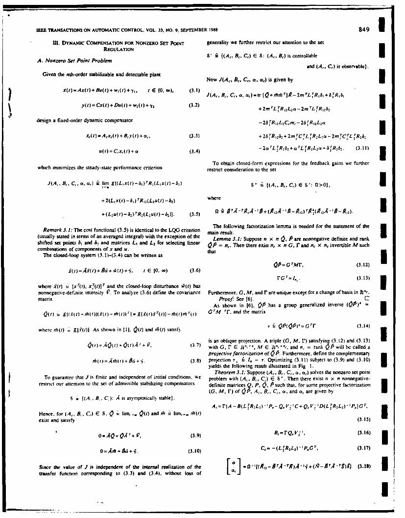
WE RNATOSON AUTMATIC CONTROL. VOL. 33. No. 9, SEPTEMBER 1988 849 IH11. DYNAMIC COMPENSATION FOR NONZERO SET POJINT generality we further restrict our attention to the set

REGULATIONS'4(ABC E :(,B)iscnrlae

A. Nonzero Set Point Problem 8 (r ~ ~ :(r ~ scnrlaland (A_. C,) is observable).

Given the nth-order stabilizable and detectable plant Now J(AC, Bc, Cc, a, a,) is given byI

;1t x t u t , 1 y . 1 1 , ) 3 1 J (A c , B , C , a . a )= tr [Q + th rh iT I 2 m T L T R ,6 + ST

1% ~~y(i) =Cx(t) +Du() + W2(1) +72 (3.2) + ZM L rR12 ~ mT R~5

design a fixed-order dynamic compensator - 26 R 2L2Ccm - 26 R12L2a

Xt)A~xc(t) + By(t)+ c, (3.3) + 26rb MT L _Lr2Tr~R4

UM )= C,x/) + a (3.4) 2 (311

To obtain closed-form expressions for the feedback gains we furtherwhich minimizes the steady-state performance criterion restrict consideration to the set

J(A,, Be, C_, a, a,) C, lim .E(xIJ)~(L~)~i (A, B,, C,) E 8': 0>0),I

" 2(Lix(t) -6)R 2 L2u(t) -62 ) where

" (L~u(I) - 6--) R(L~u(t) - 6)]. (3.5) 111 0r 74TAI~ A'0+ (9.14 A - A,) Truq(gAA 'B fil)-

Remark 3. 1: The cost functiona. (3.5) is identical to the LQG criterion The following factorization lemma is needed for the statement of themain result.3(usually stated in terms of an averaged integral) with the exception of te Lemma 3. 1: Suppose n x nt a, S are noninegative definite and rank

shifted set points 61 and 6, and matrices L, and L2 for selecting linear 0~ = n,. Then there exist n, x it G, r and nc x n, invertible M suchcombinations of components of x and u. ta

The closed-loop system (3.l)-(S.4) can be written as 0 u,(.2zIx~f +& 1 () i tE 10, co) (3.6)

where fr(t) Ix "(t), x (t)j r and the closed-loop disturbance ip~r) hasnonnegative-definite intensity V~. To analyze (3.6) define the covariance Furthermore. G, M, and r are unique except for a change of basis in 1,"..matrix Proof: See (61.C

As shown in 161, !01 has a group generalized inverse (01S)s~(f .E th(()XR([)- rftf)) I = 1Ajj(,)1r() _fh()h T(1 GM 'mr, and the matrix

w h e r r h l) 1 .i t fl . s s o w n i n I ) Q ~ ) a d r ~ t) s a t s f Nis a n o b l iq u e p r o j e c t i o n . A t r ip l e ( G , m . r') s a t i s f y i n ? ( 3 .1 2 ) a n d ( 3 .1 3 )Qht) ='40t:)+ 0t), I+ .(3,7) with G, r' E R", '", M E Wlr ",, and i, = rank Q P5 will be called a

projective factorization of ioA Furthermore, define the complementaryAm (I=Arfil)+ 86+ i. (3.8) projection r., -- i, - 7% Optimizing (3.11) subject to (3.9) and (3. 10)

yields the following result illustrated in Fig. I. -Theorem 3. 1: Suppose (A,, B_. C_, a, a,) solves the nonzero set pointI To guarantee that J is finite and independent of initial conditions. wAC problem with (A,, B_, Q E 8". Then there exist nt x nt nonnegative-

restrict our attention to the set of admissible stabilizing compensators definite matrices Q. P, C), 5 such that, for some projective factorization(GM m, ) of io 15 A,, Be, c, o, and ac are given byU

S (A, . B_, C,): A is asymptotically stable).A,= rlA - B(L R2L')-P.- Q. V 'C+ QV 'D(L R2L2 ) 'PIG T,

Hence, for (A,, B_, Cr) E 8. lim, .. 0(r) and thi lim,_.. sfr(i)Iexist and satisfy (.5

0 +Q4T+9.(3.9) B,=rQ.v21, (3.16)

Since the value of J is independent of the internal realization of E 1 IR EA TEgA -l+(R,#TA -ggJ (3.13g) 3transfer function corresponding to (3.3) and (3.4). without loss ofa]

850 IEEE TRANSACTIONS ON AUTOMATIC CONTROL. VOL. 33, NO. 9. SEPTEMBER 1988

GAI OFFETN

[- '-'TURPANCE

C,, DYNAMIC

COMPENSATOR GI

Fig. .

l5 and such that Q, P, O, and P satisfy Corollary 3.1: Let n, = n, assume (3.24) is satisfied, and suppose(Ac, Bc, C,, ci, ac) solves the fullordcr nonzcro set point problem with

O=AQ 4-QA T+ V:-QoV r'Q,7+r .Q V- tQ r ' rj, (3.19) (A,, B,, Cc) E . Then there exist n x n nonnegative-definite matrices

0:A rp+PA+LrR1L,-pr(LT r )-1P. Q. P such that A, B, C, a, and ac are given by

+7 TP(LT R2 L2 ))-P.7., (3.20) A,=A-BR;Brp-QC-VZIC+QCrV-IDR-IBT P .

O=Api+oQ A r+Qo 1,1Q r_ Q.V;Q,r. (3.21) B&=QCrV-',

O=AV+fAQ+Pr(LrR L,)-'P.-rpy(Lr2 (3.22) C,=- -R. IBTP.

rank O-rank P=rank O=n . (3.23) -'

Proof. See Section IV. 0 and such that Q, P satisfyRemark 3.2: The results of 161 are a special case of Theorem 3.1. To

see this set 61 = -Y1 = 0. 62 = 0, '2 = 0, L, = 4., and L 2 = 4., which 0=AQ+QAT+I_-CTV21CQ,

yields the results of 161 with the added features of correlated plant/measurement noise ( Vl). cross weighting (R,,), and a direct transmission 0 = A rp+ PA + R, - PBR - 1B I P.term (D) in the plant dynamics

As discussed in 16). in the full-order (LQG) case n,- = n the Lyapunov Remark 3.3: Note that by setting 6, = -y, = 0, 6 = 0, Oy= 0, and Dequations (3.21) and (3.22) for and Pare superfluous. In this case G = = 0, Corollary 3 1 yields the standard LQG result.Is I and thus G = r = = withou loss of generality. To develop Remark 3.4: It is easy to see that in the full-order case n, = n afurther connections with standard LQG theory, assume solution to the nonzero set point problem exists as long as 0 is positive

definite. In the reduced-ordcr case, however, the situation is moreL,= I.. L = l. RI: = 0. V = 0 (3.24) complex. For details, see 18).

and define IV. PROOF or THFOREM 3.1

R, 0 [R 0]o To optimize (3.11) over the open sct 8S' subject to thc constraints (3.9)

0 CrRC 0 [ and (3.10). form the Lagrangian

0 R.C [R2o 0] £(A,, Br. Cr, a, ae) tir 1),JJ(A,B,, C_. a. a,)

0 0 0 0J + ('40+ 0Ar + 17) A+ X r(Ak + AC;+5

0wheretheLagrangemultipliers kz 0, XE P'",andJ15 E P are notS[ 0 ] = C~ ]all zero. Setting al/8ti = 0 and using the fact that A is asymptotically

.rstable, it follows that ho = I without loss of generality.In this case 8 becomes Now partitioni x ii 0, P into n x n, n x n., n, x n, subblocks and

Ke E .1" into I" and t", components as((, _C)E8:0>0o Q12 ] P12.) rTAT(IA +(& 4- &_ )r6(A -- (All)- Thus, the stationarity conditions are given by

aX- AQ+ QA r+ P=o, (4.1)

A r~+ PA+ A 0,(4.2)

WME TR.ANSACTIONS ON AUTrOMATIC CONTROL. VOL. 33. NO. 9. SEPTEMBER 198

a- .,, ... + A TX +41 jfraf_0 (4.3)

I 1I2j

YA7m12 2 (4.5) 384~I I IX2 M TCT+~ 2~yT. 2sTD

FaBc 12 12 12 12I2 (4.6)

+L1R2L 2atmTr-LR 262,T+! a TXj MT= (4.

Expanding (4. 1) and (4.2) yields Substituting this expression for Ac into (4.8)-(4.13) it follows that (4. 10) 3O=AQ + IA T II + CQT QiCTB . (.8) = r(4.9) and (4.13) = G(4.12). Thus. (4. 10) and (4.13) are superfluous

O=At+iAT~j~+BQ~ 12 CT(48 and can be omitted. Next. using (4.8) + G2T(4.9)G - (4.9)G -

0= AQ 12 + Q,2A 1+ CQ 2 + Q, C2 + V 1 B r+ Q,,C!DrB r, (4) 1(4.9)GIT and G~r(4.9)G - (4.9)G - I(4.9)GITyils(.)an m(3.21). Using (4.11) + rTG(4.12)r - (4.12)r' - CR4.12)r IT and

0=AQ+,ArBQ1+QrrB+BV Tr TG(4.12)r - (4.12)r - 1(4.12)rJT yields (3.20) an (3.22).-0=AQ2 Q2 C'BC1 +QCB+yB To obtain (3.18) note that (4.4) can be rewritten as+BDC,Q2 +Q2CTDrB,', (4.10)m

CU0=A TPI+ PjA+ L rR1 Li+ C T Pr,+P 1 2 C. (4.11) 2T6 f h- f R0 (4.15)

0=A Tp 12 +P12A c+ CTB TP 2 + PBC + L R 12L 2 C, + PjzBDC , (4.12) Next, note that (4.3) is equivalent to

+CTDr T P2 +P2BDCr. (4.13) 212 (.6

Next, note that (4.4) implies that 1\2 = 0, and thus (4.5) can be written Substituting (4.16) into (4.15) yields

as PQ 2 ~ =,.(.4 (g 2-fr'A- rgr?)& + (AT.- #A- r),h + (ffA- rfg? )' . (4.17)

The existence of Q 2 and P, I follows from the fact that (A, B, C, is Netnoeha(30)ieqvlntomminimal. See [61 for details. Now define the n x n matrices W1 -A -'i&A '~ (448

Q 4=,QtQj.Q.C'QT! P PP,-1T2 Now, substituting (4. 18) into (4.17) yields

7 1 _Q2Q P,P'P (4.20.p~r4T )

and the nc x n, it x nt, and n, x nt matrices Finally, note that the coefficient of & in (4.20) is equivalent to 0 and thus

G~QQ~. M~QP 2 , '~ ~p T (4.20) yields (3.18).

Note that 7 = GT1. Clearly. Q, P, io, and Is are symmetric and V. CONCLUDING REMARKS-

nonnegative definite. The results of the present note can be combined with the results of [I I toNext note that with the above definitions, (4.14) is equivalent to (3.13) obtain nonstrictly proper controllers leading to a generalization of [7]. U

and that (3.12) holds. Hence. 7 = GTr is idempotent i.., r2 7. Current research is focused on extending the results of the present note toSylvester's inequality yields (3.23). Note also that larger classes of command and disturbance signals.

7-0 6=A.REFERENCESIThe components of Q and P~ can be written in terms of Q, P. , G,

and r' as I]) D. S Bernstein andl W. M. Haddad. "Optimal output feedback for nonraro aetpoint regulation,- IEEE Trans. Aut omat. Contr., vol AC-32. pp 641-645.Qt=Q+0. P1 =P+P. 1987

[21 H. Kwkernask and R Sivan. Linear Optimal Control Systems NewYokQ, - r rP., - JG r.Wiley. 1972.

Q,2=Qrr 2 31 Z. Artmien anid A. Leizarowitz. "Tracking periodic signals with the oveftalungjQ,.rrr ,-GO T.criterion," IEEE Trans. Automat. Comm,. vol. AC30. pp. 1123-1126. 111115. m

Q2~~rT p 2 0 ~0 ~141 A. Leizarowitz. "~Tracking nonperiodic trajectories with the overtaking crite-The xnrssins 3.1) ad (.17 folow rom(4.) ad (.7)i'. usn uon." ApAI. Moth. Oprlmiz., vol. 14. pp. 155-171. 19116.

The~~~~~~~~~ ~~~~~ exrsin 316.n.31)W utfo 46 nd(.)b sn 151 - . "Ilnfinite horizn aochestic regulation and tracking with die overtakingthe nt, and nt components of (4.4), respectively, and the above identities. criron,- Stochwasfics, 15087.Next, computing either r(4.9)-(4. 10) or G(4. 12) + (4.13) yields (3.15). (61 D. C. 8tylarid end D. S. Benitin. "Tbe optimal projection equations for fixed-

852 iEEE TRANSACTIONS ON AUTOMATIC CONTROL. VOL. 33. NO. 9. SEPTEMBER 198

order dynamic compensation." IEEE Trans. Automat. Conir., vol. AC-29, pp. where L = T - V. T and V are the kinetic and potential energies of the1034-1037. 1984. system, respectively.

[71 D. S. Bernstein. -The optimal projection equations for static and dynamic output Li p, be the ith generalized momentum 19]. Using Legender's dualfeedback: The singular cae," IEEE Trans. Automat. Contr.. vol. AC-32. pp.1139-1143. 1987. transformation

ktil S. Richter. "A hotnompy algorithm for solving the optimal projection equations p,= aL/a,, iO 1, 2, • •. (2)for fixed-order dynamic compensation: Existence. convergence and globaloptimaliy271531 in Proc. Amer. Conr. Cof., Minneapolis MN, June 1987, pp. Since L is a quadratic function in , p is linear in 0 for any given 0, i.e.,

P,= a5 () , i=1,2, .-.. (3)

with aj(9) = 82 L/8,08,

The inertial matrix is H = 182L/8 8,36,], with det (H) = h(O) > 0,Vg, wheredet (-) is the determinant of(-). Now, from (i). (2), and (3) we

A Study of Controllability and Time-Optimal Control of havea Robot Model with Drive Train Compliances and 0,= aL/M0,+ q,, i= 1. 2, ., (4)

Actuator Dynamics

A. AILON AND G. LANGHOLZ

Using (5) one obtainsAbstract-The problems of robot controllability and time-optimal

control where drive train compliances and actuator dynamics are1incorporated in the mathematical model is the subject of this note. This 8L/80,= c (6)p,p /(det (H)) 2 . (6)study demonstrates the conditions that ensure the existence of a time-optimal control, and establishes controllability of the augmented model(robot and actuator) in open- and closed-loop form. This note describes a Equations (4)-(6) constitute the state equations of the n-link mechanical

procedure for the derivation of easily computable functional inequalities system which can be written as

which represent upper bounds on the norm of the augmented system's :(t) = F(z(1)) + Bq(t). z(t0) = z (7)time response.

where the vectorsz [pTOT1r, q = [qlq2 ... q.1r, and F = [FIF2 ...I. INTRODUCTION F2 ,1r are in Euclidean vector space with the usual norm 1lz 11 = .,

To obtain the control strategy of mechanical manipulators, various (Z, 2. We also havecontrol schemes are presented in the available literature. A few examplesare resolved control [I], inverse problems technique [21, and resolved F,= cspP /[det (H) 2, s= 1, 2, , nacceleration control 131. In most cases, the control scheme involves the -Ucomputation of the appropriate generalized forces by the equation

H +d,,p, /det(H). s=n+1,n+2, ...,2nH002+ 0, 6)+ R(6,= q Iwhere 0 and q are the vectors of the generalized coordinates and forces, and B = [ ]. where I is the n x n identity matrix.

resocctively. H is the moment of inertia matrix, K is a vector specifying As an example, the exact equations for the two-link mechanical system

centrifugal and Coriolis effects, and R is a vector specifying gravitational which is confined to move in the vertical plane are given byeffects.

In much of the- literature the actuators providing the drive torques are p, = [ppzl, I m 2 sin (0,- 01) det (H)- (0.Sp'l 2 + 0.5p(+m )

modeled as pure torque sources. However, this approach is in most cases -p p2E]2EI, 2-m2 sin (02-60)]/(det (H))'a simplification of the realistic models of the system [41-[81. - (m-gIl + m2 g1j) sin 6 + q = F(p. p2. 8, 62) + q,

The objectise of this note is to studN controllability and to inestigatethe conditions which ensure the existence of a control function that p2 = -[p,p 2 ,1 4m 2 sin (02-0) det (H)-[.5p'12 +.5p( 1 ,+m,)

l transfers the augmented model of the mechanical system, the actuator'sdynamics. and the drive trains compliances. from a given initial position -ppzE]2E 1 4,mz sin (0:- 1)]/(det (H))-m.gl42 sin 0:+.q

to a desired target in a minimum time The m, ,: and the approach are = F2(pl, p.. 0, 02)+ q2useful for the design of a linear contr, .. er and can be used as a point ofdeparture for a more general model ot a robot arm. 6, = (p /-p E),,det (H) = F(p 1.p. 01, 0,)

11. THE MATHEMATICAL MODEL. 6z=(p:( 1+m 21I,)-pE)/det (H)=F,(p,, p. 6,, 0.) (8)

The Lagrange formulation of a multilink mechanical system is given by where E = 1142m 2 cos (62 - 6,). m, and 1, are the mass and the length ofthe ith link, respectively, I, is the moment of inertia of the ith link with

d(aL/O,)/dt -aL/a6, = q,, i= 1. 2 ... n (1) respect to the ith joint, and 1,, is the distance from the ith joint to the centerof gravity of the ith link.

The term det (H) is a trigonometric function of. and periodical in. 9,.Manucnpt rm.eived April 18. 1985. revised July II. 1986. April 10. 1987. and This function attains its minimum in the interval 0 S 0, s 2 , i - I, 2,

September 23, 1987. ... n, and thereforeA, Ailon is with the Depana.eni of Electrical and Compu( .'-igineering. Ben-Gunon

University of the Negev. Beer Sheva. Israel.G Langholz is with the Department of Electrical En..,eering. Florida State det (H);k>0, vt E R'. (9)

University,. Tallahassee. FL 32301IEEE Log Number 8821571 We turn now to the dynanucs of the robot's drivers. The robot is

0018-9286/88/0900-08280I.00 © 1988 IEEE

I

i July 1988

II

Optimal Reduced-Order State Estimation

for

Unstable Plants

I

i Dennis S. Bernstein Wassim M. HaddadHarris Corporation Department of Mechanical and

Government Aerospace Systems Division Aerospace EngineeringMS 22/4848 Florida Institute of Technology

Melbourne, FL 32902 Melbourne, FL 32901II

i Abstract

The problem of optimal reduced-order steady-state state estimation is considered for the casein which the plant has unstable poles. In contrast to the standard full-order estimation probleminvolving a single algebraic Riccati equation, the solution to the reduced-order problem involvesone modified Riccati equation and one Lyapunov equation coupled by a projection matrix. This

projection is completely distinct from the projection obtained in Bernstein and Hyland, 1985, forstable plants.

ISupported in part by the Air Force Office of Scientific Research under contract F49620-86-C-

0002.

I

I

1. Introduction IIt has recently been shown that optimal reduced-order, steady-state state estimators can be 3

characterized by means of an algebraic system of equations consisting of one modified Riccati

equation and two modified Lyapunov equations coupled by a projection matrix. The solution 3given in Bernstein and Hyland, 1985, however, was confined to problems in which the plant is

asymptotically stable, while in practice it is often necessary to obtain estimators for plants with

unstable modes. The purpose of the present paper is to obtain results similar to those of Bernstein

and Hyland, 1985, for unstable plants. 3Intuitively, it is clear that finite, steady-state state-estimation error for unstable plants is achiev-

able only when the estimator retains, or duplicates in some sense, the unstable modes. Roughly Ispeaking, the solution given in Bernstein and Hyland, 1985, is inapplicable to the unstable problem

for the simple reason that the range of the projection matrix may not fully encompass the unstable 3subspace. Hence, in the present paper we derive a new reduced-order solution which is constrained

to estimate all of the unstable states. Specifically, for a plant with an unstable subspace of di- 3mension n., we characterize the optimal estimator of order nu which observes all of the unstable

states. 3As in Bernstein and Hyland, 1985, the solution is given in terms of an oblique projection

(denoted in the present paper by p) which characterizes the optimal estimator gains. Again in

contrast to the lone observer Riccati equation of the standard full-order theory, the optimal reduced-

order estimator gains for an unstable plant are given by an algebraic system which, in the present Icase, consists of one modified Riccati equation and one Lyapunov equation coupled by the projection

matrix p. 1It is important to stress that the solution derived in the present paper is fundamentally different

" from the solution obtained in Bernstein and Hyland, 1985, for two reasons. First, the estimator

obtained in Bernstein and Hyland, 1985, was characterized by three matrix equations (in variables

Q, Q, and P) while the solution obtained herein involves two matrix equations (in variables Q

and P). And, second, since the projectii p arising in the present paper depends upon P, it is

completely distinct from the projection r appearing in Bernstein and Hyland, 1985, which depends Iupon Q and P. Hence the results of the present paper neither generalize, nor are a special case of,

the results of Bernstein and Hyland, 1985. 1I

I

I

In applying the results of the present paper we note that the solution is applicable to problems

in which the unstable subspace also includes additional stable modes. Indeed, the only constraint

in applying the theory is that the unstable subspace include all of the unstable poles. To clarify

this point (see Sections 2 and 3 for notation) we note that all unstable poles of A must be contained

in A., but A. may also contain an arbitrary number of selected stable poles. Thus, the estimator

derived in the present paper can be viewed as a subspace-constrained observer-estimator.

Finally, the result given herein is only a partial solution to the reduced-order estimation prob-

3 lem. Specifically, a reduced-order estimator which includes all of the unstable modes and optimal

combinations of a fixed number of stable modes should involve both projections r and p, and fotur

matrix equations in variables Q, P, , and P . When the result is specialized to the full-order case

we expect the two projections to merge to form the identity and the four matrix equations to col-

lapse to the single observer Riccati equation. A third projection v due to singular measurement

noise and static estimation can also be incorporated (Haddad and Bernstein, 1987, Halevi, 1988).

This general solution remains the subject of current research.

After introducing notation, we consider the reduced-order estimation problem for continuous-

time plants in Section 2. In Section 3 the corresponding discrete-time problem is considered. For

stable plants the reduced-order discrete-time solution was given in Bernstein, Davis, and Hyland,

1986.

Notation and Definitions

I Note: All matrices have real entriesIR, Rr x o, IRr , IE real numbers, r x s real matrices, IR' x l , expected value

I., ( )T, 0 ,x., 0, n x n identity matrix, transpose, r x s zero matrix, 0 rx.

n, , n6 , ne , n8 , q positive integers

I, Y, aX, XU, X,, yo n, 1, ne u, no, q-dimensional vectors

A, C n x n, t x n matrices

Au, Auu, A* nu x nu, n,, x no, no x n° matrices

CU, C. t x nu, I x nu matrices

L, Lu, L. q x n, q x nu, q x no matrices

R q x q positive-definite matrix3 A., B., C., Do n. x no, ne X t, q x nl, q x t matrices

t, k t E [0,oo), discrete-time index 1,2,3,...

323

II

A-[O0,1.,.]BC

w,(.), w2 (.) n, t-dimensional continuous-time or discrete-time white noise processes IV, n x n nonnegative-definite intensity or covariance of wl (-)

V2 t x t positive-definite intensity or covariance of W2 (')

V1 2 n x t cross intensity or cross-covariance of w, (-), W )

(() - -l- ] B.W2 (.)fln,n

V1 -V, 2 BT[I,, o..x.- [o.x.j[ BVx + o.,] .V [o

2. Problem Statement and Main Theorem

Reduced-Order State-Estimation Problem. Given the nth-order observed system Ii(t) = Az(t) + wi(t), (2.1)

11(t) -- OCt) + w2(t), (2.2)I

design an nth-order state estimator =

=,(t) = AeZe(t) + Bey(t), (2.3) 3Ye(t) = C.,(t), (2.4)

which minimizes the state-estimation error criterion

J(A.,B.,C.) - lim IE[Lx(t) - y. (t)]TR [Lx (t) - y,.(t)]. (2.5) 1In this formulation the plant is partitioned into possibly unstable and stable subsystems. Thus,

letting z(t) = [zT(t),zfl(t)]T and wi(t) = [wT (t), WT(t)]T , (2.1) can be written asr i (t) 1w = A us Is4 X u t) + [ 1(t) 1 (2.6)

where Au E IR"" Xn is possibly unstable, A. E IR" x,. is asymptotically stable, and the measure- 3ment equation (2.2) becomes

= [ . + W2(t). (2.7)

Furthermore, the matrix L, which is partitioned as 3L = [Lu L.], (2.8)

3

I

I

identifies the states or linear combinations of states whose estimates are desired. The dimension n,

I of the estimator state z is fixed to be equal to the order of the unstable part of the system, i.e.,

n, = n.. Thus, the goal of the Reduced-Order State-Estimation Problem is to design an estimator

of order n. which yields quadratically optimal estimates of specified linear combinations of states of

the system. As mentioned in Section 1, A, includes all unstable modes of A as well as an arbitrary

3 number of selected stable modes of A.

Since A, may contain unstable modes, define the error state z(t) _ zm(t) - x(t) satisfying

i i(t) = (A. - BC.)z,(t) - Aez.(t) + (Aus - BC,)z,(t) + w J 1 (t) - B. 2 (t). (2.9)

3 Note that the explicit dependence of the error states z(t) on the unstable states z(t) can be

eliminated by constraining

SA.u= -B.C (2.10)

so that (2.9) becomes

i(t) = (Au - B.C.)z(t) + (A, - B.C.)x.(t) + w2,(t) - B,C 2 (t). (2.11)

I Similarly, the explicit dependence of the estimation error (2.5) on the unstable states zm (t) can be

eliminated by settingC. = L. 2.12)

3 Now (2.9)-(2.11) yield

X(t) -A£(t) + tZCt), (2.13)

* wherewhe A z(t) ][Au - B.Cu Au. - BC.]

I t X '(0 0 .x .. A.

I and Z(t) and its intensity V are given in Section 1.

n To guarantee that J is finite, consider the set of asymptotically stable reduced-order estimators

S _ {(A. E,, C.): A. = Au - BCm is asymptotically stable},

so that A is asymptotically stable. Of course, S is nonempty if (Au, Cu) is detectable. Furthermore,

3 for nondegeneracy we restrict our attention to the set of admissible estimators

$+ A {(A,B,,C.) E : (A.,C,) is observable},

I

!I

Iwhere A. and C. are given by (2.10) and (2.12). Also, for arbitrary Q E ]Rfx " define the notation

Q. = QC + V 2.

Theorem 2.1. Suppose (A., B.,C.) E S+ solves the Reduced-Order State-Estimation Prob- Ilem with constraints (2.10) and (2.12). Then there exist n x n nonnegative-definite matrices Q, P

such that A., B., C. are given by

A. = O(A - Q.Vi- 1C)FT , (2.14) UB. =OQVi - ' , (2.15)

C. LF', (2.16)

and such that Q, P satisfy 3O = AQ + QAT + V1 - + _.Q.v Q°Is, (2.17)

0= (A - pQ.VjIC)TP + P(A - pQaVj- 1C) + LTRL, (2.18)

where 3PL. P. I (.9

F =4 [1.. 0..,..], - [I.. P;1 P.o], (2.20)

In. P;-1 P.A

* = J , , =0 1 -,s. (2.21)

Furthermore, the minimal cost is given by

J(A., B.,C.) = tr QLTRL. (2.22)

Proof. See Appendix A. 0

Remark 2.1. Note that since OFT = I. the nx n matrix p which couples the modified Riccati

equation (2.17) and the Lyapunov equation (2.18) is idempotent, i.e., 2 = p. Note also that rank 3p = n,,. This projection is completely distinct from the projection r appearing in Bernstein and

Hyland, 1985. 35

. . . . ,,,nm,,u~nm~uuuunnnm n~mn m nmml|NNI I n nl mm mI

Remark 2.2. In the full-order case n. = n, Theorem 2.1 corresponds to the standard steady-

state Kalman filter result. To see this, formally set - = F = u = I, and u_ = 0, so that (2.18) is

superfluous and (2.17) specializes to the standard observer Riccati equation.

Remark 2.3. Note that (2.14) and (2.16) are merely restatements of (2.10) and (2.12). Fur-

thermore, (2.15) implies that A = A - pQ.Vj 1-C so that the coefficient of P in (2.18) is asymp-

3 totically stable.

3. Discrete-Time Formulation

Discrete-Time Reduced-Order State-Estimation Problem. Given the nth-order ob-U served system

sCk + 1) = Az(k) + w(k), (3.1)

3 y(k) = cx(k) + W2(k), (3.2)

3 design an nth-order state estimator

z,(k + 1)= A.z,(k) + B,y(k), (3.3)

y,(k) = C.x.(k) + D~y(k), (3.4)

I which minimizes the discrete-time state-estimation error criterion

J(A,,B,,C,,D,) A lim IE[Lz(k) - y.(k)]TR[LZ(k) - y,(k)]. (3.5)

3 Because of the discrete-time setting it is now possible as in Bernstein, Davis, and Hyland, 1986, to

permit a static feedthrough term D. in the estimator design. The gain D. represents a static least

3 squares estimator in conjunction with the dynamic estimator (A,, B,, C.).

As in the continuous-time case, the plant is partitioned into stable and possibly unstable3 subsystems according to (2.6). Furthermore, an error state z(k) 4_ x,(k) - x.(k) is defined, A. is

constrained as in (2.10), and C. is constrained to be L, - D,C=. Thus, the augmented system

3 consisting of the error states z(k) and the stable states x.(k) becomes

3 i(k + 1) =Z,4(k) + tZ(k), (3.6)

where i(k) = [zT(k),x4(k)]T.

6

I

I

To guarantee that J is finite and to obtain closed-form expressions for the estimator gains we

restrict our attention to the sets 3{ {(A., B.,C., D.) : A. = A- B.C. is asymptotically stable},

§ {(A*,Be,Cc,Do) E 9: (A.,C.) is observable

Also, for arbitrary Q E IR" x define the notation IAQC + V1 2 , CT V2 + CQCT.

Theorem 3.1. Suppose (A,, B,, C,, D) E $+ solves the Discrete-Time Reduced-Order State-

Estimation Problem. Then there exist n x n nonnegative-definite Q, P such that A., Be, Cc, D. are

given by

A. = O(A - q.l'C)F T , (3.7)

B, = - (3.8)

C, = (L - DeC)FT, (3.9) 3D= LQCTVP". 1, (3.10)

and such that Q, P satisfy I

Q= AQA - QVt + V (3.11)

P = (A - pQa41-IC)TP(A - g V4.1-C) + (L - D.C)TR(L - D.C), (3.12) 3where F, 0, 1, and 14j. are defined by (2.19)-(2.21). Furthermore, the minimal cost is given by

J(A,,Be,Ce, Dc)= tr [(LQL r - D.V2 DT)R]. (3.13) I

Proof. See Appendix A. 0 3Remark 3.1. If a strictly proper estimator is desired, then delete D, in (3.9), (3.12), and 3

(3.13).

7 I

I

I Appendix A: Proof of Theorems 2.1 and 3.1

To analyze (2.13) define the second-moment matrix

Q(t) AIF[() (] (A.1)

which satisfies3 Q ¢(t = AQ(t) + Q()A T + f, t > 0. (A.2)

Since (A., B., C.) E S, A is asymptotically stable and

Q A lim IE[i(t)_T(t)]

exists and satisfies

0 = AQ + QA T +V. (A.3)

Next note that (2.5) can be written as

I J(A.,B,,C.)= tr QLTRL. (A.4)

To minimize (A.4) over the open set S+ subject to the constraint (A.3), form the Lagrangian

C(A., B.,C.,Q, P,A) A tr[AQL T RL + (AQ + QAT + f,")p], (A.5)

where the Lagrange multipliers A > 0 and P E IR'fxfl are not both zero. Setting 8.C/aQ 0, A = 0

I implies P = 0 since A is asymptotically stable. Hence, without loss of generality set A = 1.

3Now partition n x n P into n. x n,, n, x n,, and n. x n. subblocks as

I P-PZP.' °

Thus the stationarity conditions are given by

3,_ = rp + PA + LT RL = , (A.7)aq

... = PB.V - [P. P.](QCT + V12) = 0. (A.8)

3Expanding the n,, x n,, subblock of (A.7) yields

0 = (A. - B.CI)TP + PU(A. - B.CU) + L TRLU, (A.9)

8I

I

which, using (2.10) and (2.12), is equivalent to m

O =ATP. + P.,A. + C.,RC.. (A.10) m

Thus, since (A., B.,C.) E $+, (A.,C.) is observable and it follows from (A.10) that P, is positive

definite. Since P is thus invertible, define the n, x n matrices

F [In. O. xn..], 4' - [In. P;,P,], (A.11) m

and the n x n matrix p A F 0. Note that since OFT - 1n, p is idempotent, i.e.,, 2 = .

Next note that (A.8) and (A.11) imply (2.15). Similarly, (2.14) is equivalent to (2.10) with B.

given by (2.15). Finally, (2.16) is a restatement of (2.12). Now, using the expression for B,, A andVbecome

A = A - 1Q.V'C, (A.12) l

V-= V VI - QGVj-*V +aQoVj"QrpT. (A.13)

Finally, (2.17) and (2.18) follow from (A.3) and (A.7) using (A.12) and (A.13).

For the discrete-time problem define the second-moment matrix IQ(k) 2 IE[i(k)i T (k)],

which satisfies Qk + ) = AQ(k)A T + V. A.14)

Since A is asymptotically stable,

Q lim IE[:(k)ET (k)]

exists and satisfies

Q = AQA T + . (A.15)

The remainder of the proof follows as above for the continuous-time case.

Acknowledgment. We wish to thank David C. Hyland for several helpful suggestions.

I9 I

I

I

i References

Bernstein, D.S., and Hyland, D.C., 1985, IEEE Trans. Autom. Contr., AC-30, 583.

Bernstein, D.S., Davis, L.D., and Hyland, D.C., 1986, AIAA J. Guid. Contr. Dyn., 9, 288.

Haddad, W.M., and Bernstein, D.S., 1987, IEEE Trans. Autom. Contr., AC-32, 1135.

Halevi, Y., 1988, "The Optimal Reduced-Order Estimator for Systems with SingularMeasurement Noise,' preprint.

IIi

IIIIIII

I

I APP IX L: Discrete-Tim Theory

I 41. D. S. Bernstein, L. D. Davis and D. C. Hyland, "The OptimalProjection Equations for Reduced-Order, Discrete-Time Modelling,Estimation and Control," AIAA J. Guid. Contr. Dyn., Vol. 9, pp.288-293, 1986.

44. D. S. Bernstein, L. D. Davis and S. W. Greeley, "The OptimalProjection Equations for Fixed-Order, Sampled-Data DynamicCmpensation with Ccuputation Delay," IEEE Trans. Autom. Contr., Vol.AC-31, pp. 859-862, 1986.

I 54. W. M. Haddad and D. S. Bernstein, "The Optimal Projection Equationsfor Discrete-Time Reduced-Order State Estimation for Linear Systemswith Multiplicative White Noise," Sys. Contr. Lett., Vol. 8, pp.381-388, 1987.

69. D. S. Bernstein and W. M. Haddad, "Optimal Projection Equations forDiscrete-Time Fixed-Order Dynamic Compensation of Linear Systems withMultiplicative White Noise," Int. J. Contr., Vol. 46, pp. 65-73,1987.

I 92. D. S. Bernstein, "Inequalities for the Trace of Matrix E"ponentials,"SIAM J. Matrix Anal. Ap=1., Vol. 9, pp. 156-158, 1988.

I 87. D. S. Bernstein, "Cnm~uting Matrix Exponentials," Problem 88-1, SIAMRey , Vol. 30, p. 123, 1988.

128. D. S. Bernstein and C. V. Hollot, "Robust Stability for Sampled-DataControl Systems," Amer. Contr. Conf., Pittsburgh, PA, June 1989.

IIIII

298 J. GUIDANCE VOL. 9, NO. 3

I1 The Optimal Projection Equations for Reduced-Order,

Discrete-Time Modeling, Estimation, and Control

I Dennis S. Bernstein,* Lawrence D. Davis,t and David C. HyilandtHarris Corporation, Melbourne, Florida

IThe optimal projection equations derived previously for reduced-order, continuous-time modeling. estimation.and control are developed for the discrete-time case. The design equations are presented in a concise, unifiedmanner to facilitate their accessibility for the development of numerical algorithms for practical applications. As inthe continuous-time case, the standard Kalman filter and linear-quadratic-Gaussian results are immediatelyobtained as special cases of the estimation and control results.

INomenclature I. Introduction

A. R, C - nX n,nX m,*X n matrices N a recent series of papers"" it has been shown that the-n ×n n× m, x n matrices r necessar, conditions for quadratically optimal,A,B,.,, - nX n., nX m,txnmatices con tinuous- time, reduced-order modeling. estimation, and

A,B,, C', D, - n, X n,, n, &, p X n, p X &I matrices control can be transformed into coupled systems of two, three,iA,. B,. C,. ), - n, X i , n X , m × n, m X ?- matrices and four matrix equations respectively. this coupling, due to

E, - matrix with unity in the (i, i) position the presence of an oblique projection (idempotent matrix),and zeros elsewhere arises as a rigorous consequence of optimality, hence suggest-

E -expected value ing the name optimal projection. For the estimation andI, - r X r identity matrix control problems, this formulation provides a direct generali-k - discrete-time index 1,2,3.... zation of classical steady-state Kalman filter and linear-L -p X n matrix quadratic-Gaussian (LQG) control theory. In the full-ordern, m, -, n,, I case the projection becomes the identity matrix, the additional

n,. n,. p - positive integers, 1 !5 n_, n,, n, s n two modified Lyapunov equations drop out, and the remain-R, N, R - t- x -, p X p, m x m positive-definite matrices ing modified Riccati equations become the usual Riccati equa-R - n X n nonnegative-definite matrix u.ions.

R1, -n x m matrix such that R -R 2 1 2R12 Coupling via the optimal projection supports the view thatis nonnegative definite sequential reduced-order design procedures consisting of either

RR" real numbers, r x s real matrices 1) model reduction followed by estimator (controller) designR, R2 or 2) estimator (controller) design followed by estimator (con-

RTr R2 troller) reduction are generally not optimal. Furthermore, fortr Z - trace of square matrix Z the control problem the coupled structure of the equations

. y.. - m-, t-. p-dimensional vectors yields the further insight that in the reduced-order case thereV m x m positive-definite covariance of w is no longer separation between the operations of state estima-V n x n nonnegative-definite covariance of wi tion and state-estimate feedback. i.e.. the certainty equivalenceV- e x e positive-definite covariance of w2 principle breaks down.V1. n n x / cross-covaiance of i ,. w, For practical applications, the optimal projection equations

.: - m-, n-, (-dimensional zero-mean discrete-time permit the development of alternative numerical algorithmswhite noise processes that operate through successive iteration of the optimal pro-

x, x, x,. x - n-, n_,-, n,-, n,-dimensional vectors jection4" rather than by gradient search techniques.' 2 ByZ - (a, j) element of matrix Z recognizing that each local ex tremalcorresponds to n, possibleI -transpose of vector or matrix Z choices out of n rank-I eigenprojections of the product of aZ-T (ZT)- 1 or (Z- i )T pair of pseudogramians. it is possible to efficiently identify the-,(,) ,E,- 1 (unit-rank eigenprojection'7 ) global minimum.' 0 This idea is philosophically similar to

p(Z) - rank of matrix Z Skelton's component-cost analysis. 15

The purpose of the present paper is to develop the optimalprojection equations for reduced-order modeling, estimation,and control in the discrete-time case. Since the tnderlyingtheory has been discussed previously,' the presentationherein is geared toward a clear and concise statement of the

Received April I. 1985; revision received Aug. 26. 1985. Copyright main results to facilitate numerical developments and practi-C American Institute of Aeronautics and Astronautics, Inc., 1986. All cal application. For example, by expressing the optimal pro-rights reserved.

*Associate Principal Engineer, Controls Analysis and Synthcsis jection in terms of eigenprojections, a variety of novel al-Group Government Aerospace Systems Division. gorithms are immediately suggested. For illustrative purposes

tLead Engineer, Controls Analysis and Synthesis Group, Govern, we apply the results on reduced-order state estimation to ament Aerospace Systems Division. Member ALAA third-order problem to obtain reduced-order estimators and

*Principal Engineer, Controls Analysis and Synthesis Group the results on reduced-order dynamic compensation to aGovernment Aerospace Systems Division. Member AIAA. tenth-order problem to obtain reduced-order controllers.I

MAY-JUNE 1986 REDUCED-ORDER MODELING, ESTIMATION, AND CONTROL 289

Because of the discrete-time setting it is now possible to For the fixed-order dynamic-compensation problem, a staticpermit static feedthrough gains in the estimator and controller feedthrough term is included, i.e., the controller may be non-designs. As previously noted,' nonsingular control weighting strictly proper.and measurement noise in the continuous-time case permitonly a purely dynamic (strictly proper) controller. Note that Reduced-Order Dynamic-Compensation Problem

this is precisely the case in continuous-time LQG theory, Given the controlled systemwhich always yields a strictly proper feedback controller. Thestatic gains in the discrete-time estimator problem permit x(k + 1) -Ax(k) + Bu(k) + w(k) (11)simultaneous, unified treatment of nondynamic least-squares v(k) - Cx(k) + w2(k) (12) Iestimation along with dynamic (Kalman filter-type) estima-tion. design a reduced-order dynamic compensator

The references include a representative sampling of paperson quadratically optimal reduced-order modeling. 2

5estima- x(k - (Ak) + B(k,tion. 5 3" and control, 4 '4 along with closely related ap- (k Iproaches. For emphasis on the discrete-time problem, see u(k) = C,x,(k) + D,(k) (14)Refs. 18. 30, 41. 42, 4, and 45.

Il. Problem Statement and Main Results which minimizes the dynamic-compensation criterion

We now state the reduced-order modeling, estimation, and J,(A,, B, ,C.,O,) A m E[x(k)TRx(k)control problems. The object of the model-reduction problem -

is to determine a model of reduced state-space dimension )TRk (whose steady-state response to white noise inputs (or, equiv- +2x(k ) u(k) + u(k) IRu(k)] (15)alently, impulse response) best approximates, in a quadratic

(least-squares) sense, the response of a given high-order sys- To guarantee that J,,, J,, and J, are finite and independenttem. In the reduction process the order of the reduced model of initial conditions, consideration is restricted to the follow-is fixed and the optimization is performed over the .iodel ing (open) sets. [A triple (.4, B, C) is min nal if (A, B) is Iparameters. controllable and (A, C) is observable.]

Reduced-Order Modeling Problem ., - A ,, ,, C.

Given the modelx( k + 1) - Ax(k) + Bw( k) (1) A., is stable and ( A, B, C,) is minima)

y(k) - Cx(k) (2) V,-{(A,,,C,,D,):

design a red' -ed-order model A, is stable and (A,, B, C) is minimal) 3x.,(k + 1) -A.x_,(k) + B.w(k,) (3) Y A- (A,, B,,,C, D,)

y.(k) - C,,x(k) (4)4 + BD,.C BC,

which minimizes the model-reduction criterion B C A, J is stable and ( A, , B.. C, ) is minimal,

J_,A_,. B,.CJ) Let n, genericall- denote n,., n,. and n,. The following

factorization lemma will be needed for the main results-" im El .,( k)-y(k)] -R[y.(k) -y(k)] (5) L.emma 2 ,1 Let 7 CR '". T h en

The goal of the reduced-order state-estimation problem is to - r (16)design an estimator of given order which yields quadraticallyoptimal (least squares) estimates of specified linear combina- p() -n, (17)

tions Lx of states x In practice, the order of the estimatormay be determined by implementation constraints, such as if, and only if, there exist G, r ( R"", such thatreal-time computing capability. Note that the feedthrough Iterm D, permits the utilization of a static least-squares esti- GrF -r (18)mator in conjunction with the dnamic estimator (A, B,, C, I.

Reduced-Order State-Estimation Problem rGr _ 1,, (19)

Given the observed system Furthermore, G an - are unique to a change of basis in R".

x( k + 1) - Ax( k) + w,( k) (6) Proof SufficiencN s obvious. To prove necessity, first notethat due to Eq (16) the eigenvalues of -r are either 0 or I

.(k) Cx(k) + %,(k) (7) Further, it is easy to see that r has a diagonal Jordan Icanonical form Hence, the result follows from

design a reduced-order state estimatorx,( k+ 1) - Ax,{k) + By( k) (8) 0rslo 0O -r

.y,(A) - Cx,( k) + Dy( k) (9)

which isiirumizes the state-estimation criterion where G- t r 01ST.I -[,-i 01S , and FR .'... aFor convenience, call G and r satisfying Eqs, (18) and (19)

Ji A_ 8,. C,, D,) a projecte facruri:anon of r. Furthermore, for n X n non-

negative-definite matrices (i.e., symmetric matrices with non-lir E v,( k) - Lx( k)] T NJ y,( k) - Lx( k)] (10) negative eigenvaues) .R and 9. define the set of contragpedi-

290 BERNSTEIN, DAVIS, AND HYLAND J. GUIDANCE

ently diagor aizing transformations and such that Q, ), and P satisfy9(_-.,) Q -AQA*-(AQCr+ v,2) f'(AQCT + v"2)'

3= RAx : - -r and rg* are diagonal) (31)_v 1Y (31)

It follows from Ref. 48, p. 123, Theorem 6.2.5, that 9(.f,9) "- A r TAT + (32)is always nonemptY. This set does not, however, have a unique

element since basis rearrangements and sign transpositions A - A~riPAQ + 1. (33)may be incorporated into t. Further nonuniqueness aris if

£9 has repeated eigenvalues. whcreTheorem 2.1. Suppose A is stable and (A,.,B1,C, ._ where

solves the reduced-order modeling problem. "Tben there exist ",n X n nonnegative-definite matrices Q and P such that A., v." I,(t) (34)B_, and C., are given by,-

I,.adC aegvn A, - rAGT (20) for some *r9(QP) such that (0'Qt*)(,,) 0, i-I . n, and some projective factorization G,r of -. Further-

B, - ra (21) more, the minimal cost is given byI~C -,.CG r (22) .A.,,B.,-C,,D,) -tr[( LQLr - D.'D N](

and such that Q and + satisfy For the control result, define the additional notation

Q-AOlAr+ BVBT (23) A (AQCr+ V, + BDflz 2 (AQCr+ V2, + BD,) r

p-Ar. pA+Cr A24 X (BpA + R" + ,DcC)r1t-(BrpA +Rr + kD¢C)IPA~r71A + CTRC (24) T

I where AA A - BkRt(BTPA + R 2 )

I--iA~f,* (25) RA R,+ BrPB

for some 'I'E3(QP) such that ( 1-Q*) *0, i" MAI 'n ]' kA[-;1(BPA+Ri

1..n, and some projective factorization GF4f f. Fur-thermore, the minimal cost is given by Theorem 2.3. Suppose (Ar, BE, C,, D,) EY, solves the re-

duced-order dynamic-compensation problem. Then there existJ.,( A,., B.,, C.) - trl( W - ,T)cTRc (26) n x n nonnegative-definite matrices Q, P. Q, and P such that

(2) A,, B, C , and D, are given byanPsuhtt

where :.; is the unique (nonnegativeefinite) solution of A, - r [ A - ( AQC r + V, CI W -A W Ar + B V~r - B -'( BrpA + RT ) - BD ClG r 36

~~~A+2B 12 (36)

For convenience in stating the estimator result, define the B, - r[( A QCT + V12) ,pi + D,] (37)notation

+ ) DC

C - -[ z'(BTPA + Rr) + DC] CTIQ A ( AQC r + V,2 ) Pi '( AQC r + V12 )T 129 . -R ' rp ~ r ~ B pV2) ' ( 9

IQ.(AQ+VI)V~AQCD,2 - -. k-L(BrPAQCT+ Rr QCT+ BTPv )fr' (39)

p AA-DC)( VD.C) and such that Q, P, Q, and P satisfy

AQ A (AQC + VQ)1 C Q - AQAT - (AQCT + V,2) f- (AQ C r + V)T

+ V, + .CQ)

A 1, 1 (40)

Theorem 2.2. Suppose A is stable and (A,, B,,PC,, D,)AC 12 2 +,

solves the reduced-order state-estimtion problem,. Then there + R, + rr (

exist n X n nonnegative-definite matrices Q, Q, and P such

that A, B,., C,, and D, are given by Q - A ,rOTTA+ (42)

A , - r [ A - ( A Q c T + v 1, ) i C ] G T ( 2 7 ) I AP<i' 1 'A + ! ', ( 4 3 )

D,- r(AQCr+ v,)-' (28) where

S, -( L - C)G T (29) for n,() (44)

Dot-some ,fo( om)such that ("- ) 1 #,,)*O. i.- LQCr V (30) .n,, and some projective f[(wrization c, r 4 r. Further.I

IMAY-JUNE 1986 REDUCED-ORDER MODELING, ESTIMATION, AND CONTROL 291

more, the minimal cost is given by augrmented Lyapunov equation and its dual. The interesting 1

aspect is that the explicit gain expressions and the definitionJ, (A,, B, C,. D,) - tr[( MQMT + A;frrr, fT) k] (45) of the optimal projection arise in the reverse order as com-

pared to the continuot, ti: derivation. Similar remarks applyRemark 2.1. To specialize the estimation and control results to the reduced-order modeling and estimation problems.

to the strictly proper (no-feedthrough) case, merely ignoreEqs. (30) and (39) and set D,- 0 and D, -0 wherever they BI. Examplesappear. As an application of Theorem 2.2 on reduced-order state

Remark 2.2. In the full-order cases n, - n and n, -n in estimation, the stirred-tank example from Ref. 36, pp. 107.Theorems 2.2 and 2.3, the projection r becomes the identity 473, and 531, is considered. Ignoring the undisturbed volumeand Eqs. (32), (33), (42), and (43) plav no role. In this case G state, the remaining states are the incremental tank concentra-and r are also the identity. Specializing further to the purely tion and variations in the feed concentrations. The problemdynamic case D, = 0, D, -0 as in the previous remark yields data are as follows:tle standard Kalman filter and LQG results.

Remark 2.3. As previously noted." 1.11 the indeterminacy in [0.9048 0.06702 0.022621specifying the projective factorization G. I' satisfying Eqs. (18) A - 0.8825 0 1and (19) corresponds to nothing more than an arbitrary choice 0 0 0.9048 1of internal state-space basis for the design systems(A_.. B,.C,,),(A.,, C,), and(A,.B,.C). C_[1 0 01,oV 10-6, V1 0, N'L -1

Remark 2.4. Since and P are balanced by means of thetransformation '1 - (Q, ), it follows that *'-'QP ' is di- 5.399X 10-6 8.015 x 10- 8.762 x 10-'agonal. Hence, QP is semisimple and thus fl,(,) is a rank-1 V, | 8.015 x 10- 2.212 x 10 Ieigenprojection of QP. (A semisimple mat ix possesses a L8.762X×10-5 0 7.251 × 10-3'diagonal Jordan form."4 67' ) Although the optimal projection 'ris characterized in Eqs. (25). (34). and (44) as the sum of The standard Kalman filter result isrank-i eigenprojections of QP. because of the nonuniquenessin Q(Q. P). the theorems do not specify which eigenprojec- [ -0.7959 0.06702 0.22621

tions actually comprise r. From analytical examples" it can 4, = [ 8.205 0.8825 0 l

be seen that each of the (n) possible projections may corre- I.-10.29 0 0.9048spond to a local extremal in the optimization problem. [ 1.701 1

Remark 2.5. The proofs of Theorems 2.1-2.3 are similar to Bo= 18.205the continuous-time results and, hence, have been omitted. To [10.29 lhelp the reader reconstruct the lengthy manipulations, the keydetails differing from the continuous-time case are pointed C, = 13, D,-0out For the control problem. an (n + n, ) X (n + n,) discrete-time algebraic Lyapunov equation is obtained for the steady- with performance J, - 0.0358515.state covariance of the closed-loop system. Regarding this Permitting nonzero feedthrough D,, yieldsequation as a side constraint, the Lagrange multiplier tech-nique is used to compute stationarity conditions that yield [ 0.09885 0.1061 -0.0167 1 [-13.34 1explicit expressions for A,, B,. C,. and . The projection A, -0.6851 0.02176 0.09015] , B,- -10.08 Iarises %%hen these expressions are substituted into the original [ 0.1503 0.2652 0.8707 J 1 2.2371

- 0.006261 -0.007282 0.00074450.5716 -0.0002166 0.007202 ],0.6822 -0.006021 -0.005440

D_10.9068O,,= 9.298/

11.37 1-, 1 where the (improved) performance is J, = 0.032401049.For the reduced-order results, an algorithm for solving allthree equations (31-33) is described briefly. Begin by setting

r - I,, and solving Eqs. (31-33) for the "full-order" values of1 Q. Q. and P. Choose n, eigenprojections of QP in diagonal-

izing coordinates and iterate the modified Lyapunov equations(32) and (33) until convergence of r, Q, and P is obtained.t " Return to Eq. (31) and solve for Q With V + T , as the

new nonhomogeneous term in the Rliccati equation. Repeatthe above steps until convergence is reached.

In applying this algorithm to the present example, theeigenprojections were chosen for convenience in accordancewith the largest eigenvaues of QP. The results indicate attain-ment of the globai minimum. For the optimal second-orderfilter, the gains are given by

A,- 10.09898 -0.1137 ] 9713.3310.6632 -0.02285 9.7621

S[-0.006259 0.007796 [.081

Fig. I Ro4. mI p- we po ,ma on rorArt-mode 0.5716 -0.00027371 , - 9.298 /beam *%am* 0.6823 0.006121 J L11.37 J

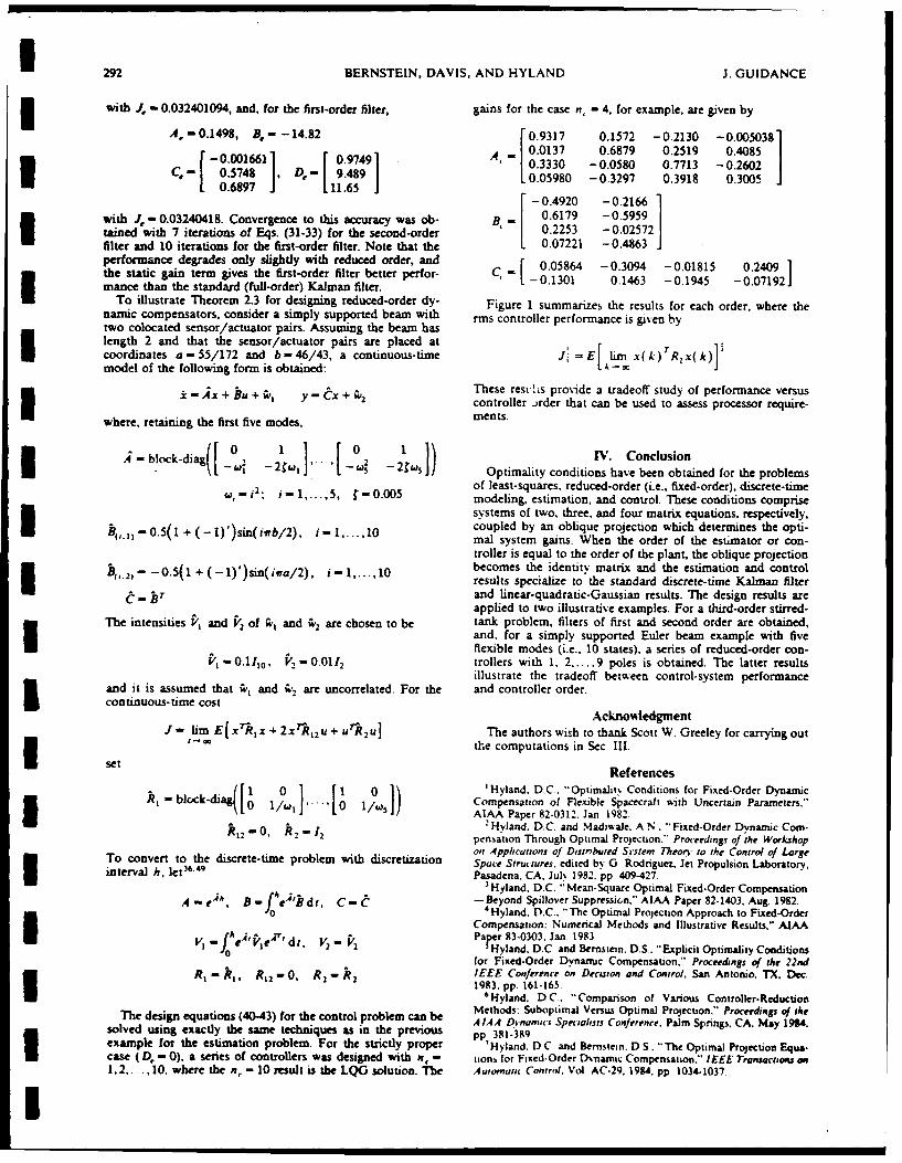
292 BERNSTEIN, DAVIS, AND HYLAND J. GUIDANCE

with J, - 0.032401094, and, for the first-order filter, gains for the case n, - 4, for example, are given by

A,-0.1498, B- -14.82 [0.9317 0.1572 -0.2130 -0.0050381A 0.0137 0.6879 0.2519 0.4085

-0.001661 D 0.9749 A 0.3330 -0.0580 0.7713 -0.2602 /C,-[ 0.5748 6 , D, 9.489 L0.05980 -0.3297 0.3918 0.3005 J

0.6897 1.65 1 -0.4920 -0.2166I0.6179 - 0.599

with J, -0.03240418. Convergence to this accuracy was ob- B,tained with 7 iterations of Eqs. (31-33) for the second-order 0.2253 -0.02572

filter and 10 iterations for the first-order filter. Note that the 0.07221 -0.4863performance degrades only slightly with reduced order, and [ 0.05864 -0.3094 -0.01815 0.2409 1the static gain term gives the first-order filter better perfor- C -0.1301 0.1463 -0.1945 -0.07192Jmance than the standard (full-order) Kalman filter.

To illustrate Theorem 2.3 for designing reduced-order dy- Figure 1 summarizes the results for each order, where thenamic compensators, consider a simply supported beam with rms controller performance is given bytwo colocated sensor/actuator pairs. Assuming the beam haslength 2 and that the sensor/actuator pairs are placed atcoordinates a -55/172 and b - 46/43, a continuous-time J =E[ linx(k)rR,x(k)'model of the following form is obtained:

These rest-ls provide a tradeoff study of performance versus,4x + Bu + ; i y - ex + C., controller order that can be used to assess processor require-

where, retaining the first five modes, ments.I ([~0 1 0 ')c..o4 - blcsck-diag([0 1 1 [o H IV. Conclusion

-2 c. ..... '-, -2 s.JJ Optimality conditions have been obtained for the problems

i . of least-squares. reduced-order (i.e., fixed-order), discrete-time-- 0.005 modeling, estimation, and control. These conditions comprise

systems of two, three, and four matrix equations. respectively.,,,-0.5(1 + (-))si(ib/2), i-1,...,10 coupled by an oblique projection which determines the opti-

mal system gains. When the order of the estimator or con-troller is equal to the order of the plant, the oblique projectionbecomes the identity matrix and the estimation and control-0.5(1 +(1)')sin(ira/2), i- 1_ _10 results specialize to the standard discrete-time Kalman filter

e 11T and linear-quadratic-Gaussian results. The design results areapplied to two illustrative examples. For a third-order stirred-

The intensities V, and V2 of 4', and ,2 are chosen to be tank problem, filters of first and second order are obtained,and, for a simply supported Euler beam example with fiveflexible modes (i.e., 10 states). a series of reduced-order con-

'l 0.111 , "2 -00112 trollers with 1, 2.....9 poles is obtained. The latter resultsillustrate the tradeoff between control-system performance

and it is assumed that 4,1 and iiz are uncorrelated. For the and controller order.continuous-time

costJ - lim E| x 7Rx + 2xrR, 2 u + urR2u] The authors wish to thank Scott W. Greeley for carrying out

set -the computations in Sec. III.

set References

S 0 1 01 'Hyland. D.C.. "Optimalit% Conditions for Fixed-Order Dynamicblock-diag 0 / . Compensation of Flexible Spacecraft with Uncertain Parameters."I tIW5J AlAA Paper 82-0312. Ian 1982.

-0, R, - I2 Hyland. D.C. and Madiwale. AN.. "Fixed-Order Dynamic Com-k212 pensation Through Optimal Projection." Proceedings of the Workshopon 4ppicatons of Distributed Sistem Theori to the Control of Large

To convert to the discrete-time problem with discretization Space Structures, edited by G Rodriguez, Jet Propulsion Laboratory.interval h, let 6 .4 9

Pasadena. CA. Jul. 1982. pp 409-427.3 Hyland. D.C. 'Mean -Square Optimal Fixed-Order Compensation

A - e", B - e'B d t, C - -- Beyond Spillover Suppression." AIAA Paper 82-1403. Aug. 1982.f0 4 Hyland. D.C.. "The Optimal Projection Approach to Fixed-Order

Compensation: Numencal Methods and Illustrative Results," AIAAPaper 83-0303. Jan 1983V, - f e "' Pef r' drt, V2 P2 PHyland. D.C and Bernstein. D.S. "Explicit Optimality Conditions0 for Fixed-Order Dynamic Compensation." Proceedings of the 22nd

R1 - k 1, R12 -0, R2 1 k2 IEEE Conference on Decwon and Control, San Antonio. TX, Dec.1983. pp. 161-165

'Hyland. DC. "Comparison of Various Controller-ReductionMethods: Suboptimal Versus Optimal Projection," Proceedings of theThe design equations (4043) for the control problem can be A IAA Thnamics Specilhsts Conference. Palm Springs, CA. May 1984.solved using exactly the same techniques as in the previous pp 381-389

example for the estimation problem. For the strictly proper 7Hyland. D C and Bernstein. D S. "The Optimal Projection Equa-case ( D, - 0), a series of controllers was designed with n. - tions for Fixed-Order DXnaminc Compensation." IEEE Tranwsactotu on1.2.. .10. where the n, - 10 result is the LQG solution. The Autornatn Control. Vol AC-29. 1984. pp 1034-1037.I

I.MAY-JUNE 1986 REDUCED-ORDER MODELING, ESTIMATION, AND CONTROL 293

"Hyland. D.C. and Bernstein, D.S. "The Optimal Projection Ap- °'Fairman. F.W., "Reduced Order State Estimators for Discrete-proach to Model Reduction and the Relationship Between the Meth- Time Stochastic Systems," IEEE Transactions on Automatic Control,ods of Wilson and Moore." Proceedings of the 23rd IEEE Conference Vol. AC-22. 1977, pp. 673-675.on Decision and Control, La Vegas, NV, Dec. 1984, pp. 120-126. 31Sims, C.S. and Asher, R.B., "Optimal and Suboptimal Results in

'Bernstein. D.S. and Hyland, D.C.. "The Optimal Projection Equa- Full- and Reduced-Order Linear Filtering." IEEE Transactions otions for Reduced-Order State Estimation," IEEE Transactions on Automatic Control, Vol. AC-23, 1978. pp. 469-472.Automatic Control, Vol. AC-30, 1985, pp. 583-585. 32Wilson, D.A. and Mishra, RN.. "Design of Low Order Estima-

'i

Hyland. D.C. and Bernstein, D.S.. "The Optimal Projection tors Using Reduced Models." International Journal on Control, Vol.Equations for Model Reduction and the Relationships Among the 23. 1979, pp. 447-456.Methods of Wilson, Skelton and Moore," IEEE Transactions on 33Dombrovskii. U.V., "Method of Synthesizing Suboptimal Filters 1Automatic Control, to appear. of Reduced Order for Digital Linear Dynamic Systems," Av-tomatioe,

"Bernstein. D.S. and Hyland. D.C., "The Optimal Projection and Remote Control. Vol. 43, 1982, pp 1483-1489.Equations for Finite-Dimensional Fixed-Order Dynamic Compensa-tion of Infinite-Dimensional Systems," SIAM Journal on Control and 34Johnson. T.L. and Athans, M., "On the Design of OptimalOptimization, to appear. Constrained Dynamic Comapensators for Linear Constant Systems,"

'2 Looze, D.P. and Sandell. N. R. Jr., "Gradient Calculations for IEEE Transactions on Automatic Control, Vol. AC-15. 1970, pp. 658-Linear Quadratic Fixed Control Structure Problems," IEEE Transac- 660.tions on Automatic Control, Vol. AC-25. 1980, pp. 258-285. 35Levine. W.S.. Johnson, T.L.. and Athans, M.. "Optimal Limited

"3

Skelton. R.E.. "Cost Decomposition of Linear Systems with Ap- State Variable Feedback Controllers for Linear Systems.- IEEEplication to Model Reduction," International Journal on Control, Vol. Transactions on Automatic Control, Vol. AC-16, 1971. pp. 785-793.32. 1980. pp. 1031-1055. 3'Kwakernaak. K. and Sivan. R., Linear Optimal Control Systems,"'Skelton. R.E. and Yousuff, A.. "Component Cost Analysis of Wiley-lnterscience. New York. 1972.

Large Scale Systems." International Journal on Control, Vol. 37, 1983, 37Rom. D.B. and Sarachik. P.E.. "The Design of Optimal Corn-pp. 285-304, pensators for Linear Constant Systems with Inaccessible States,"

'iYousuff, A. and Skelton, R.E. "Controller Reduction by Compo- IEEE Transactions on Automatic Control, Vol. AC-18, 1973, pp. 509-nent Cost Analysis." IEEE Transactions on Automatic Control, Vol. 512.AC-29. 1984. pp. 520-530. 3 Sidar. M. and Kurtaran. B.Z.. "Optimal Low-Order Controllers

iAMitra. D.. "Analytical Results on the Use of Reduced Models in for Linear Stochastic Systems." International Journal on Control, Vol.the Control of Linear Dynamical Systems." Proceedings of lEE, Vol. 22, 1975, pp 377-387.116. 1969. pp. 1439-1444.

" Wilson. D.A.. "Optimum Solution of Model-Reduction Problem," "Mendel, J1. and Feather. J.. "On the Design of Optimal Time-Proceedings of lEE. Vol. 117, 1970, pp. 1161-1165. invariant Compensators for Linear Stochastic Time-Invariant Sys-

"'Applevich. J.D.. "Approximation of Discrete Linear Systems," tems." IEEE Transactions on Automatic Control. Vol. AC-20, 1975. pp.International Journal on Control, Vol. 17, 1973. pp. 565-575. 653-657. I

"Wilson. D.A.. "Model Reduction for Multivariable Systems," "°Basuthakur. S. and Knapp. C.H.. "Optimal Constant ControllersInternational Journal on Control, Vol. 20. 1974. pp. 57-64. for Stochastic Linear Systems," IEEE Transactions on Automatic Con-

2°Hickin. J. and Sinha, N.K., "Applications of Projective Reduction trol. Vol. AC-20. 1975. pp. 664-666.Methods to Estimation and Control," Journal on Cybernetics, Vol. 8, "Asher. R.B. and Durrett, J.C., "Linear Discrete Stochastic Control1978. pp. 159-181, with a Reduced-Order Dynamic Compensator," IEEE Transactions on2 t

Mishra. R.N. and Wilson, D.A., "A New Algorithm for Optimal Automatic Control, Vol. AC-21. 1976. pp 626-627

Reduction of Multivariable Systems," International Journal on Con- "2 Naeije. W.J. and Bosgra. O.H.. "The Design of Dynamic Corn-trol. Vol. 31. 1980. pp. 443-466. pensators for Linear Multivariable Systems," 1977 IFAC. Fredricton,

'" Kabamba. P.T., "Model Reduction by Euclidean Methods." Jour- Canada. pp. 205-212.nal of Guidance and Control, Vol. 3, 1980, pp. 555-562. 4Wenk. CT and Knapp. C.H.. "Parameter Optimization in Linear

"Moore. B.C.. "Principal Component Analysis in Linear Systems: Systes w.t Arbitrap Cnstr a e t e r truton IEEE

Controllability. Observability, and Model Reduction." IEEE Transac- Systems with Arbitrarily Constrained Controller Structure." IEEElions on Automatic Control. Vol. AC-26, 1981. pp. 17-32. Transactons on .4itoac Control. Vol. AC-25, 1980, pp. 496-50

:' Eitelberg. E., "Model Reduction by Minimizing the Weighted "O'Reilly. J '"Optimal Lov-Order Feedback Controllers for Linear

Equation Error." International Journal on Control. Vol. 34, 1981. pp. Discrete-Time S-stems." Control and Dynamic Systems, Vol. 16, edited

1113-1123 by C.T. Leondes. Academic Press. New York. 1980, pp. 335-367.25Sims, CS. "Reduced-Order Modelling and Filtering," Control IGrimble. M I. "Reduced-Order Optimal Controller for Discrete-

and Dvnamic Sistems. Vol. 18, edited by C.T. Leondes, 1982, pp. Time Stochastic Systems." Proceedings of FEE. Vc,. 127, 1980, pp. 355-103. 55-63

2"Simon. KW and Stubberud, A.R., "Reduced Order Kalman 'Kabamba. PT. and Longman. R.W., "An Integrated Approach to

Filter." International Journal on Control. Vol. 10. 1969. pp. 501-509. Reduced-Order Control Theor%." Optimal Control Applications and27Sims. CS. and Melsa, J.L., "Specific Optimal Estimation." IEEE Methods, Vol. 4. 1983. pp. 405-415

Transactions on Automatic Control, Vol. AC-14. 1969. pp. 183-186. 4Kato, T.. Perturbation Theon" for Linear Operators, 2nd Ed.,2"Asher. R.B.. Herring. K.D., and Ryles, I.C.. "Bias Variance and Springer-Verlag. New York. 1976

Estimation Error in Reduced Order Filters." Automatica. Vol. 12, 4'1Rao. C.R. and Mitra, S.K.. Generali:ed Inverse of Matrices and Itt

1976. pp. 589-600. Applications. John Wiley & Sons. New York. 1971.29Gados. J.1. and Gustafson, D.E.. "Information and Distortion in 9Van Loan, C.F.. "Computing Integrals Involving the Matrix

Reduced-Order Filter Design." IEEE Transactions on Information Exponential." IEEE Transactions on Automatic Control. Vol. 23, 1978.Theory. Vol. IT-23. 1977. pp. 183-194. pp. 395-404

IIII

IEEE TRANSACTIONS ON AUTOMATIC CONTROL. VOL. AC-3I. NO, 9. SEPTEMBER 1916 859The Optimal Projection Equations for Fixed-Order Samon 00';0' . .,a... , -

Sampled-Data Dynamic Compensation withComputation Delay C N^.

DENNIS S. BERNSTEIN. LAWRENCE D. DAVIS, AND PROCESSOR ." i., " C.,,.0

SCOTTr W. GREELEY

Abstract-Far an LQG-Iype sampled-data regulator problem whichaccounts for computational delay and utilizes an averaging A/D device, ACTUATORG !4 S, !

the equivalent discrete-time problem is shown to be of increased order dueto the inclusion of delayed measurement states. The optimal projectionequations for reduced-order, discrete-time compensation are applied tothe augmented problem to characterize low-order controllers. The design I I I Iresults are illustrated on a tenth-order flexible beam example. R,-11, A.

Fig. I. Timing diagram for sampled-data controller..3 1. INTRODUCTIONClassical sampled-data control theory has been extensively developed ZT, Z- r transpose of vector or matrix Z, (Zr) - I

111-171 and is widely used in practical applications. Sampled-data design E, matrix with unity in the (i, i) position and zerosbased upon modern optimal control theory has also been developed, elsewherealthough to a considerably lesser extent [8]-1141. The goals of the present E, R, R x'r expected value, real numbers, r x s real matricesnote are twofold. First, for an LQG-type sampled-data regulator problem stable matrix matrix with eigenvalues in open unit diskwhich explicitly accounts for computational delay, we obtain an equiva- nonnegative- diagonalizable matrix with nonnegative eigenvaluesII lent discrete-time problem (Theorem 2.1 and Corollary 2.1). The timing semisimple 118], 119]diagram in Fig. I illustrates the unavoidable delay in the feedback loop matrix(see Section 11 for notation). A salient feature of this problem is that 01, M, , !,e positive integers, I s n, :s n + Irather than replace the continuous-time white noise measurement model x, u, y, X, n, m, /, ne-dimensional vectorsb) a discrete-time version (which is often done in the literature since A. B, C n x n, n x m. I x n matricescontinuous-time white noise cannot be sampled). we employ an averag- A,. Bc, C,, D, n, x n,, n, x I, m x nc, m x I matrices

* ing-type A/D device as in 18, p. 821 [see (2.5)]. wi, w2 n, i-dimensional zero-mean continuous-time whiteThe second goal of the note is to present a novel design procedure noise processes

which is applicable to the equivalent dicrete-time problem, and which V, n x n nonnegative-definite intensity of w,thus directly accounts for the delay effects. Since the discrete-time model I x I' positive-definite intensity of w2is of augmented order n + I(n = number of plant states, I = number of it x 1 cross intensity of w, 2

measurements), it seems natural to seek dynamic feedback of reduced R, n x n nonnegative-definite state weighting matrixorder. To this end. we apply the optimal projection equations for discrete- R, m x m positive-definite control weighting matrixtime dinamic compensation to the equivalent discrete-time problem to R n x m cross weighting matrix such that R, -characterize optimal controllers of order n, -s n + I. These equations, R12R -R T is nonnegative definite

RR2 1 2 snneaiedfntwhich were previously derived in [171 for the continuous-time case, are k discrete-time index, 1, 2, 3, .

discussed in [15]. 1161. Note that, in practice, the computational delay(and. hence, sample interval) in real-time controller implementation in the statement of the sampled-data control problem the sampledepends directl) upon the controller order n,. For example, by reducing interval h and the controller order n, are fixed and the optimization isn, the sample rate can effectively be increased. Thus, the engineering performed over the controller parameters (A,, B_, C,, Dc). For designtradeoffs of performance versus controller order and sample interval can tradeoff studies h and n, can be varied and the problem can be solved forbe investigated using the results of this note. each pair of values of interest.

This note also includes formulas for integrals of matrix exponentialsarising in the sampled-data/discrete-time conversion, along with an Fixed-Order, Sampled-Data Dynamic-Compensation Problemalgorithm for solving the optimal projection equations. The results areapplied to a tenth-order flexible beam example. Given the nth-order continuous-time system

x(t) = Ax(t) -Bu(t) + wi(t) (2.1)II. SAMPLED-DATA PROBLEM AND EQUIVALENT DISCRETE-TIME

FORMULATION with continuous-time measurements

The following notation and definitions will be used throughout. y(t) = Cx(t) + Du(t) + w2(t) (2.2)1, 0,,,, 0, r x r identity matrix, r x s zero matrix, 0,, design an nth-order discrete-time compensator

I ", (i, j) element of matrix Zx,(k+ l) = A~x(k) + B,(k ), (2.3)

ManuSCril1 received t(kiolier 4. 1985; re% used May 12., 1986. This work was supported (k+1=Ax,- +B k.(23

64--015. F49620-mb-c-OW2. and F49520-C-MW ei(k)=Ccx,(k)+ D,(k). (2.4)The authors are %Ih Ihe Controls Analyst. and Synthesis Group. Govenment

Aero4ic System% Division, Harris Corpration. Melbournc. Ft. 32902 which, with A/D averaged measurementsIEEE Log Number K609872For simplicit, the timing diagram Fig I applie s to the case in which the 96

comnpentaor isStricil) Pt'Opcr in thL note the results are stated for the more general Case fi(k) 6- y(t) dt (2.5)in wtnch a direct (siiW feedthrough term bf(A) is included h IM

U018-9286/86/0900-0859S01.00 © 1986 IEEE

IT

"60 IEEE TRANSACTIONS ON AUTOMATIC CONTROL. VOL. AC-31, NO. 9. SEPTEMBER 1986

and D/A zero-order-hold controls given by (10.9). (8, p. 831: R(, R(2, and R1 are given in [10]. [12]; andV, V'2, and Vi can be found in [8, p. 851. The expressions for 6 and D'

u(t)=jg(k), t E [kh, (k+ I)h), (2.6) appear to be new.

Note that the averaged measurements depend upon delayed samples of 3minimizes the performance criterion the state. By augmenting the discretized state equation (2.8) to include

these measurements, it is possible to state the original sampled-dataJ(A,, B,. C,, D,) limE- problem as a discrete-time problem.Corollary 2.1: With the notation 3

" xs)rRxs)+2xlslRus)+us)rRu(s)] ds. (2.7)A' 0_ ] B'

The main result of this section concerns propagation of the plant and L Adigitized measurements over one time step. For notational convenience,define w 10,. ,.' '(k) '(1 [ V ;2..... 1,1. Ck)v.-

H(s) e 4r dr.

Theorem 2.1: For the fixed-order, sampled-data dynamic-compensa- ,R ,1 0..1 12 [ j R.a

tion problem, the plant dynamics (2. 1), averaged measurements (2.5) and 1 ..

performance criterion (2.7) have the equivalent discrete-time representa- the fixed-order, sampled-data dynamic-compensation problem is equiva- itions lent to the following discrete-time problem. Given the (n + I)th-order

x'(k + I)=A'x'(k) +-B'(k) + w;(k), (2.8) discrete-time system 2

fi(k) = C'x'(k- 1) + D'a(k- 1)+ wa(k- 1), (2.9) 2(k+1)=,2(k)+ 1(k)+'(k) (2.11)

J(A,. B, C, D,)=6+ lim E[x'(k)rRx'(k) with discrete-time measurements

+ 2x'(k) rR ,2f(k) + f(k) TR24(k] (2.10) fi(k) = (k) (2.12)

design an nth-order discrete-time compensator of the form (2.3), (2.4),where which minimizes

x'(k) & x(kh). 6 - 1 tr eA, R dr ds, J(A e, Be, Cc, De)=6 +lim E[.f(k)T i (k)0 0 , b A--m

A' A BID + 2 (k)TA ,2 af(k)+ 0(k)rg 2a (k). (2.13)

A"'=• ". B" !aHlhlB, C' 9- CHlh), D' - 1 C H~s) dsB +D;h Remark 2.1: The equivalent cost (2.13) involves a constant offset 6

which serves as a lower bound on the sampled-data performance, i.e., aw1'(k) and wi(k) are zero-mean, white noise processes with "discretization floor." Note that

](k) L](k) 6=- tr VR,+O(h2 ).E wi(k) wi(k) V12 TV2

where Remark 2.2: Although the measurements fi(k) are noise free. the 3singularity is not so serious as singular measurement noise in the

; el V, eA ds, V, ell V. HT(s) dsCT+! H(h) Via, continuous-time case where the Kalman filter gains are expressed in terms0 1 of the inverse of the measurement noise intensity. In the discrete-time

case, rather, it is required that r + CQ-C be invertible, where P- is theV2 P 2 I measurement noise covariance (see [g, p 5301, or [151, [16]).h h 2 H(s) V. H r(s) dsC Remark 2.3: The increase in plant order from n to n + I is due to the

computational delay and A/D process. Since discrete-time LQG theory' 2-" Iyields a possibly unwieldy 'n + I)th-order controller, we seek "reduced- m

C His) dsV1,7 + IV r H r(s) dsC r, order" controllers. Note that in this context an nth-order controller can be

regarded as being of reduced order.

and Remark 2.4: As pointed out in [10], particular choices of the sampleinterval h may result in a loss of controllability and observability for the

h r ~.se R' IrI equivalent discrete-time problem. Hence, these properties must bee Ple- ,s, R;2 eArR,H(s) dsB+l HT (h)R,2 , verified before applying control design methods.

I , III APPLICATION OF THE OPTIMAL PROJECTION EQUATIONS TO THESR. + I Hr(s)R.H(S) dsB EQUIVALENT DISCRETE-TiME PROBLEM

We now apply the optimal projection equations for discrete-time+hBr H r($) dsR.,+ i R, r H(s) dsB. dynamic compensation to the equivalent discrete-time problem. The

dsR 22+ E following easily proved lemma will be needed.

The proof of this theorem is a straightforward calculation involving Lemma 3.1. Let r E 1 Then

standard techniques, and hence is omitted. The result is more comprehen- = 7. (3.1)sive than previous work, however, and includes several results as specialcases. For example, the expressions for A' and B' are standard; C' is AT) = n, (3.2)

IiIEEE TRANSACTIONS ON AUTOMATIC CONTROL. VOL. AC-31. NO. 9. SEPTEMBER 1986 861

3 if and only if there exist G, r E Rlexnt- ) such that given by

GrI=r, (3.3) J(A,. Be, C., D,)=6+tr ((MQMr+lRrarrrT)AI. (3.14)

rG r J,,,. (3.4) Remark 3.1: Theorem 3.1 can immediately be specialized to the morerestrictive problem in which the compensator is strictly proper. This can

Furthermore. G and r are unique to a change of basis in R"c. be done in both the full- and reduced-order cases by ignoring (3.8) and

Call G and r satisfying (3.3), (3.4) a projectivefactorization of 7. setting D, - 0 wherever it appears. See [15], [16].Furthermore. for n x n nonnegative-definite matrices Q and 61, definethe set of ccntragrediently diagonalizing transformations IV. NUMERICAL EVALUATION OF INTEGRALS INVOLVING MATRIX

e( . ) L, (1 E R"x t-IQ+-T and *, T") are diagonal). EXPONENrIALS

It follows from 119, Theorem 6.2.5. p. 123] that e(Q. 6) is always To evaluate the exponential/integral expressions appearing in Theoremnonempty. This set does not, however, have a unique element since basis 2. 1, we utilize the approach of [20]. The idea is to eliminate the need forrearrangements and sign transpositions may be incorporated into i. integration by computing the matrix exponential of appropriate blockFurther nonuniqueness arises if 4QT has repeated eigenvalues. matrices. Numerical matrix exponentiation is discussed in 121).

To guarantee that J is finite and independent of initial conditions, we Proposition 4.3: Consider the following partitioned matrix exponen-

restrict our consideration to the (open) set tials of order (3n + 1) x (3n + 1). (3n + m) x (3n + m), (2n + m)x (2n + m), and (3n) x (3n). respectively:

S(A, B, C, D) A + ADC AC] F F2 F, F, 1 xp [ A 1. 0. ,,{(c 8- ,J1. Fs F6 F7 0. -A VI V2

0. 0. Fs F, 0. 0. Ar Cr

is stable and (A,, B, C) is minimal} 0 o t. 0 1.. 011. [/ 0 . . 01. 0

For the design problem it is required that £ be nonempty, i.e., that the F, F F,2 F 1 [ Ar i, 0. , 1augmented system be stabilizable. We also require the notation [ 0. FF, Fl t exp 0, -A. R R h.

0 0. FF exp 0. A B

21., 2 12 [F . Fig F,1 [ 0A . 0.1.M 2 oA-i , 0. F F, exp 0. -A V h.

2 F2 F2 1 . 0I

LD_'cJ [ PA + 12 0. 026 F., J 0. 0 A V

Theorem 3. 1: Suppose (A, B, C, D) E S solves the fixed-order, A'=F, B'-=Fn, C'=! F r D'- CF,+D, 6=- tr RIFT F5,

sampled-data dynamic-compensation problem. Then there exist (n + I) A

x (n + ) nonnegative-definite matrices Q. P, 0, and such tha( A, V I r)B. C,, and D, are given by V1'=FrF, -V, FrF, V2=! + aCFIF + FrFsC),

A,:rIA-AQCT17-'i-BAi'(grpA+Rr,)-,#D< IGT, (3.5)i

SR,' FF,, R[2='F,6 , R ,=R2+ (BrFrF,,+F,,B).3,=r1A 1 ' r +,#D, (3.6)

C,- = - iA- l(ATPA + A1 De ,]GT (3.7) V. NUMERICAL SOLUTION OF THE DiSCRETE-TIME OPTIMALPROJECTION EQUATIONS

D,-= _j-I(B9TpAQeT+.r QCT )7-, (3.8)

and such that Q, P. 0, and P satisfy The following algorithm is proposed for solving (3.9)-(3.12).

Algorithm 5.1:Q=AQA _ AQC P. ICQA " + ,, (3.9) Step 1: Initialize k = 0 and r') = 4,.,.

Step 2: With 7- A 701 solve (3.9)-t3.12) for Q(-) i Q. P"I 9 P,12( 3 P 0.10) i 0. and fr*k - A

(3.1or I) JStep 3: If k ; I check for convergence: If II(Q4; Pt), (k), P0k))

_=A(Q(k -,, pSt ep, :. 1 1 -I ), _ - on > to] then continue; else go(3=A2) to Step 6.

whe ~re~.2 Step 4: Select * E (k'', pEk*) and update 7.1"'I)where *, (k)E,( , (k)) - 1.

Step 5: Increment k and go to Step 2.11Step 6: Evaluate (3.5)-(3.8) with Q = Qlh*, p _ p~k). Q _ 0thI,

( E1 - (3.13) =Phi) GrTJ , h) rGT = J..

Remark J.: In solving the Riccati equation (3.9), the nonhomoge-for some *E 42(i. P)such that (0-iaP*),.l 0,i i, - ., and neous trm is taken to be IP + 7, 0rrT which is nonnegative definite.some projective factorization G. r of T. Furthermore, the minimal cost is Si tilar remarks apply to (3.10).

N62 IEEE TRANSACTIONS ON AUTOMATIC CONTROL. VOL. AC-31. NO. 9. SEPTEMBER 1986

TABLE I continuous-time systems 1221. 1231: robust sampled-data control ofCOST J FOR BEAM EXAMPLE uncertain systems with multiplicative noise 1241-[271; multirate sampling 1

128). 1291; alternative A/D and D/A devices and asynchronous sampling/

SSU C ' control update, infinite-dimensional systems 1301, 1311.g

1 1 REFERENCES

12 - 1.3715 3.0134 111 J. R. Ragazzini and G. F. Franklin. Sampled-Data Control Systems. New IYork: McGraw-Hill. 1959.

10 1.1677 1.3723 3.0134 121 E. I. Jury. Sampled-Data Control Systems. New York: Wiley: 1958.131 J. T. Tou. Digital and Sampled-Data Control Systems. New York: McGra%,-Hill, 1959.

8 1.1883 1.3823 3.0162 (4) A. I. Munroe. Digital Processes for Sampled Data Systems. New York:Witty'. 1962.

6 1.2086 1.421 3.0195 [51 B. C. Kuo. Analysis and Synthesis of Sampled-Data Control Systems.Englewood Cliffs. NJ: Prentice-Hall. 1963.

4 1.3330 1.5752 3.0812 [61 D. P. Lindorff. Theory of Sampled-Data Control Systems. New York: Wiley.1964.

2 1.4789 2.0425 3.3406 [71 G. F. Franklin and J D Powell. Digital Control of Dynamic Systems.Reading. MA: Addison-Wesley. 1980.

1[ K. J. Astrom. Introduction to Stochastic Control Theory. New York:Opts-Loop Cost N-0) is 101.73 Academic. 3970.

191 A. H. Levis. M. Athans. and R. Schlueter, "On the behavior of optimal linear Isampled-data regulators." Int. J. Contr., vol. 13. pp. 343-361, 1971.

[10] P. Dorato and A. Levis. "Optimal linear regulators: The discrete case." IEEETrans. Automat. Contr., vol. AC-16. pp. 613-620. 1971.

[111 K. Kwakernaak and R. Sivan. Linear Optimal Control Systems. New York:Remork 5.2: The critical step of Algorithm 5. 1 is the choice of , (k) for Wiley. 1972.

constructing the projection rk +n Since 'tkl caninclude basis rearrange- [121 N. Hal o and A. K. Cagla~an. "A separation theorem for the stochastic sampled-data LQG problem." Int. J. Contr., vol. 23. pp. 237-244. 1976.

merts, the choice of it 0 essentially corresponds to a Selection ofn rank- 131 E.S. Armstrong and A. K. Caglayan. "An algorithm for the weighting matrices inI eigenprojections out of n + I possible eigenprojections. This selection the sampled-data optimal linear regulator problem." NASA Langley. Hampton.is discussed at length in [22] where it is pointed out that the choice of VA. Rep. NASA TN D-8372. 1976.cigenprojections determines which local extremal will be reached by the 114l T. Mita. "Optimal digital feedback control systems counting computation time of

control laws." IEEE Trans. Automat. Contr., vol. AC-30. pp. 542-548. 1995.algorithm. Component-cost methods have thus been utilized as a 1151 D. S. Bernstein. L. D. Davis. S. W Greeley. and D. C. Hyland. "The optimalpromising selection criteria. Because of the eigenprojection structure of projection equations for reduced-order, discrete-time modelling, estimation andthe necessary conditions, Algorithm 5.1 is fundamentally different from control." Proc. 24th IEEEConf. Dec. Conir., Fon Lauderdale. FL. Dec. 1985.gradient search methods. pp. 573-578.

1161 D. S. Bernstein. L. D. Davis. and D, C. Hyland, "The optimal projection

equations for reduced-order, discrete-time modelling, estimation and control." J.Guid. Contr. Dynam., vol. 9. pp 288-293. 1986.

VI. ILLUSTRATIVE EXAMPLE: CONTROL OF A FLEXIBLE BEAM [171 D. C. Hyland and D. S. Bernstein. "The optitmal projection equations for fixed-order dynamic compensation." IEEE Trans. Automat. Contr.. vol. AC-29. pp,

Consider a simply supported beam of length two with two colocated 1034-1037. 1984.sensor/actuator pairs placed at coordinates a1 = 55/172 and a2 = 45/43. 181 T. Kato. Perturbation Theory for Linear Operators. 2nd ed. New York:Springer-Verlag. 1976Define [191 C. R Rao and S. K Mirra. Generahzed Inverse of Matrices and Its

Applications New York: Wile). 19710 1 ] 1201 C. F. Van Loan. "Computing integrals involving the matrix exponential." IEEE

A =block-diag it02 i-I , 5, r=0.00, Trans. Automat. Contr.. vol AC-23. pp. 395-404, 1978.2., 1211 C Moler and C. Van Loan. "Nineteen dubious ways to compute the exponentialL of a matrix." SIAMRe-., vol 20. pp 801-836, I

c m1221 D. C Hyland and D. S. Bernstein. "The optimal projection equations for model

Bsji=0.-)S( )( +(- 1)') sin (ira.4), reduction and the relationships among the methods of Wilson. Skelton. andMoore". IEEE Trans. Automat. Contr.. vol AC-30. pp 1201-1211. 1985

10, j= 1, 2. C=Br, [231 - . .'The optimal projection equations for reduced-order state estimation,"IEEE Trans. Automat. Contr., vol AC-30. pp 583-585, 1985.

[24] D. S. Bernstein and D C Hyland, "Optimal projection/maximum entrop)stochastic modelling and reduced-order design synthesis." in Proc. IFACV =block-disag Vt2 =0, V:--.1 I:, Workshop on Model Error Concepts and Compensation, Boston, MA. June

0 1 1985[251 - "The optimal projectiontmaximum entropy approach to designing low-

order, robust controllers for flexible structures." in Proc. 24th IEEE Conf.F1 olDecision Contr.. Fort Lauderdale. FL. Dec. 3985. pp. 745-752.

R, =block-diag 1 0 . =0. R2=0.112. [261 - ."The optimal projection equations for reduced-order modelling, estimation,.i , L a_

0 w = O. and control of linear systems with Stratonovich multiplicative white noise.'

submitted for publication1271 A. R. Tiedeann and W. L. DeKoning, "'The equivalent discrete-time optimal

For n, = 10, 8, 6, 4, 2 continuous-time controllers were designed using control problem for continuous-time systems with stochastic parameters." Int. J.Contr.. vol 70. pp. 449-466. 1984.the results of 117] and, for n, - 12, 10, 8, 6, 4, 2 and h - 0.1, 0.5, (281 D P. Glasson. "A new technique for multirate digital control design and samplestrictly proper (D, - 0) discrete-time controllers were obtained from rate selection." J. Guid. Contr. Dynam., vol. 5, pp 379-382. 1982.

Theorem 3.1. The results are summarized in Table 1. 1291 M Araki and K. Yamamoto, "'Multivariable multirate sampled-data systemsState-space description, transfer characteristics, and Nyquist critervn.' IEEETrans. Automat. Contr., vol AC-31. pp 145-1,4, 1986

1301 M J Balas. "The structure of discrete-time finite-dimensional control ofVII. DIRECTIONS FOR FURTHER DEVELOPMENTS distributed parameter systems." J. Math. Anal. Appl., to be published.1311 D S. Bernstein and D C Hyland. "The optimal projection equattios for finite-The following extensions and related developments immediately dimensional fixed-order dynamic compensation of infinite-dimensional systems."

wggest themselves: reduced-order, discrete-time modeling/estimation of SIAM J. Contr. Optimi.., vol. 24. pp. 122-151. 1986.

....m l 1 Il l lE

I

I Systems & Control Letters 8 (1987) 381-388 381North-Holland

IThe optimal projection equations

I for reduced-order, discrete-timestate estimation for linear systemswith multiplicative white noiseUWassim M. HADDAD3 Mechanical Engineering Department, Florida Institute of Technology, Melbourne, FL 32901, USA

Dennis S. BERNSTEIN *Harris Corporation, Government Aerospace Systems Division, MS 22/4842, Melbourne. FL 32902, USA

I Received 2 July 1986

Abstract: The optimal projection equations obtained in [2,3] for reduced-order, discrete-time state estimation are generalized toinclude the effects of state- and measurement-dependent noise to provide a model of parameter uncertainty. In contrast to the singlematrix Riccati equation arising in the full-order (Kalman filter) case, the optimal steady-state reduced-order discrete-time estimator ischaracterized by three matrix equations (one modified Riccati equation and two modified Lyapunov equations) coupled by both anoblique projection and stochastic effects.

Keywords: Reduced-order Kalman filter, Robust estimation.

3 1. Introduction

In a recent series of papers [1-3] it has been shown that the first-order necessary conditions for optimalcontinuous and discrete-time reduced-order state-estimation can be transformed into coupled systems ofthree matrix equations (one modified Riccati equation and two modified Lyapunov equations). Thecoupling is due to the presence of an oblique projection (idempotent matrix) which arises as a rigorousconsequence of the stationarity conditions. This formulation provides a direct generalization of theclassical steady-state Kalman filter theory. Specifically, in the full-order case, the projection becomes theidentity matrix, the additional two modified Lyapunov equations drop out, and the remaining modified

Riccati equation reduces to the standard observer Riccati equation for the Kalman filter expression.Related results in reduced-order estimator design can be found in [4-17].

An ,a!,ntional extension of classical state estimation involves the inclusion of state- and measurement-dependent disturbances [18-24]. One motivation for such a model is to design estimators which aredesensitized, i.e., robustified, to actual parameter variations [25-31]. For the continuous-time controlproblem this has been justified in [32-38].

As shown in [36] for the continuous-time case, applying the optimal projection approach to themultiplicative white noise model yields an extended formulation of the optimality conditions for reduced-order state estimation. Specifically, the system of three matrix equations characterizing the optimalestimator are now coupled by both the oblique projection and stochastic effects.

3 Supported in part by the Air Force Office of Scientific Research under contract F49620-86-C-0002.

0167-6911/87/$3.50 D 1987, Elsevier Science Publishers B.V. (North-Holland)3I

I

382 W.M. HaddaA D.S. Bernstein / Optimal projection equations for state estimation

The purpose of the present paper is to provide a self-contained derivation of the optimality conditionsfor reduced-order state estimation in the presence of both state- and measurement-dependent white noisein the discrete-time case. The goal of the development is to present the optimality conditions in a clear,concise manner to facilitate the development of numerical algorithms for practical application. I2. Notation and definitions

R, R " , RF, E real numbers, r X s real matrices, R" , expectation.I, ( )T, g n X n identity, transpose, Kronecker product [39]._"L I. - T , r" E R x

n, m, 1, ne, q positive integers, 1 < n, < n.X, Xe n, ne-dimensional vectors. IY, Ye 1, q-dimensional vectors.A, A, ; C, C n x n matrices, I l n matrices, i = 1. p.Ae, Be, Ce, De nx Xn,, nXI, qxne, qX I matrices. Ik discrete-time index 1, 2, 3,....vi(k) unit variance white noise, i- 1 ..., p.w(k), w2 (k) n-dimensional, I-dimensional white noise processes.

V1 n X n nonnegative-definite covariance of w,(k).V2 / x I positive-definite covariance of w 2(k).V 2 n X I cross-covariance of wl(k), w2(k).R q x q positive-definite matrix. IL q X n matrix.

ABC A,] ' [B C, 0] = .~

[ k)], V, V 2 Be]LBew 2(k) B.VI Be V2B '

LrRL - LTRDC - CTDTRL + CTDTRDC + C C, DT"RD C, -LTRCe + CTDTIRC 5CTRL + CTRDC CTRC,

ZO,,j) (i, j) element of matrix Z.P(Z) rank of matrix Z. Itr Z trace of a square matrix Z.E, square matrix with unity in the (i, i) position and zeros elsewhere.

IF(4) ')E, ,-' (unit-rank eigenprojection). I.V(Z), Wi(Z) null space, range of matrix Z.

An asymptotically stable matrix is a matrix with eigenvalues in the open unit disk; a nonnegative-defi-nite matrix is a symmetric matrix with nonnegative eigenvalues; and a positive-definite matrix is a Isymmetric matrix with positive eigenvalues.

For arbitrary n X n, Q, Q, ,define

p pV2CQ2,')T -A -VQCT + CT

V2 A V2 + CQCT + LC,(Q+ C')T, Q,&AQC + V12 + EA,(Q+ ')C ,T.

I

3 IV.M. Haddad D. S. Bernstein / Optimal projection equations for state estimation 383

3. Problem statement and main theorem

Reduced-Order State-Estimation Problem. Given the n-th-order observed system

x(k+1)= A+ ui(k)A x(k)+wl(k) , (3.1)

y(k)= C+ Ev() x(k)+ w2(k), (3.2)

design an n,-th reduced-order state estimatorxe(k + 1) =Aexe(k) + Bey(k), (3.3)

ye(k) = C,,xe(k) + Dey(k), (3.4)

I which minimizes the state-estimation error criterion

SJ(Ao, Be, C., D.) A lim E[Lx(k) -y,(k )ITR[Lx(k) -y,(k)]. (3.5)

k "o

In this formulation the matrix L identifies the states, or linear combinations of states, whose estimatesare desired. The order ne of the estimator state xe is determined by implementation constraints, i.e., by thecomputing capability available for realizing (3.3), (3.4) in real time. Note that the feedthrough term Dpermits the utilization of a static least squares estimator in conjunction with the dynamic estimator(A , Be, C.). Thus, the goal of the Reduced-Order State-Estimation Problem is to design an estimator ofgiven order that yields quadratically optimal (least squares) estimates of specified linear combinations ofstates.

To guarantee that J is finite assume that A is asymptotically stable and consider the set of1 asymptotically stable reduced-order (i.e., fixed-order) estimators

y'A ((Ae, . CBe, De): Ae is asymptotically stable).

Since the value of J is independent of the internal realization of the transfer function corresponding to(3.3) and (3.4), without loss of generality we further restrict our attention to the set of admissibleestimators

3 ."y A { (A,, Be, C,, De) E6 Y: (Ar, B,) is controllable and (Ac, C) is observable}.

The following factorization lemma is needed for the statement of the main result.

I Lemma 3.1. Let r e R"". Then

T 2-- T', (3.6)

p(T) = n, (3.7)

if and only if there exist G, F E R" ×" such that

GTF = T, (3.8)

3 f rGT=I,. (3.9)

Furthermore, G and 1 are unique to a change of basis in R" .

II

U384 W M. Hadd44 D.S. Bernstein / Optimal projection equations for state estimation 3Proof. See [31. 0

For convenience, call G and F satisfying (3.8) and (3.9) a projective factorization of r. Furthermore, for 3n X n nonnegative-definite matrices and P, define the set of contragrediently diagonalizing transforma-tions- {4 R")-: f *(=- -R and pT)) 4 are diagonal} UIt follows from Theorem 6.2.5, p. 123 of [40], that 1(6, AP) is always nonempty. This set does not,however, have a unique element since basis rearrangements and sign transpositions may be incorporatedinto 4. Further nonuniqueness arises if &P has repeated eigenvalues.

Theorem 3.1. Suppose A is asymptotically stable and (A., Be, Ce, D:) (- Y + solves the Optimal Reduced-Order State-Estimation Problem. Then there exist n X n nonnegative-definite matrices Q, Q and P such thatAe, Be, C and D. are given by

A e = F(A - QSVC)GT, (3.10)

Be = FQsFV', (3.11)

Ce = (L - DC)G, (3.12)

De = LQCTV2i-, (3.13)

and such that Q, Q and P satisfyQ.._ + r T T-VIQ .IT +. T , (3.14

Q=AQ T EA,(Q t -iQ )Ai + v (3.14)1-

.= A _'TAT +QSV iS QC, (3.15)

P= (A -T~r(A - Qyi'C) + (L - D R(L - DC ), (3.16)

where 3T E' lr(4,) (3.17)

i-l I

for some 4, E (Q , fl) such that (07-1QP).') ) 0, i=1. n, and some projective facrorization G, V ofT. Furthermore, the minimal cost is given by

J( A, B , Ce, De) = tr[( LQLC - DV2 D T)R]. (3.18) 1Remark 3.1. It is useful to note that (3.10) can be replaced by I

A, = FAGT - BCCGT. (3.10)'

Remark 3.2. Because of (3.9) the n X n matrix r which couples the three equations (3.14)-(3.16) is 3idempotent, i.e., T

2 = T.. In general, this 'optimal projection' is an oblique projection (as opposed to an

orthogonal projection) since it is not necessarily symmetric. It should be stressed that the form of theoptimal reduced-order estimator (3.10)-(3.13) is a direct consequence of optimality and not the result ofan a priori assumption on the structure of the reduced-order estimator.

Remark 3.3. To specialize the result to the strictly proper (no feedthrough) case, merely ignore (3.13) andset D, = 0 wherever it appears.

II

W M. Haddad A.S. Bernstein / Optimal projection equations for state estimation 385

Remark 3.4. Replacing x. by Sxe, where S is invertible, yields the 'equivalent' estimator(SA.S - ', SBe, CeS -1 , D.) with J(SAS - 1 , SBe, CS - 1 , De)=J(Ae, Be, Ce, De). Note that transforma-tion of the estimator state basis corresponds to the alternative factorization T = (S-TG)T(sr).

Remark 3.5. Note that for the optimal values of Ae and Be the estimator dynamics (3.3) assume the usualobserver form

xe(k + 1) = 1AGTx, + FQ.Vi;'(y - CGTxe). (3.19)

By introducing the quasi-full-state estimate i A GTx, E R" so that T.i = and x= F G R%", (3.19) canbe written as

.rc(k + 1) - TAT + rQsVJ-'(y - C!). (3.20)

Although the implemented estimator (3.19) has the state x e ' R'i', (3.19) can be viewed as a quasi-full-orderestimator whose geometric structure is entirely dictated by the projection - and the stochastic effects.Specifically, error inputs QV 2 Q 1(y - C1) are annihilated unless they are contained in [ X'('r)] = q(T

) .

Hence, the observation subspace of the estimator is precisely 9?(T ).

Specializing Theorem 3.1 to the noise-free case Ai = 0, C, = 0, i = 1. p, yields Theorem 2.2 of [2,31.Alternatively, specializing Theorem 3.1 to the full-order case n. = n reveals that the Lyapunov equation forP is superfluous. In this case it follows from Remark 3.4 that G = F = I, without loss of generality.

Corolary 3.1. Assume n, = n, A is asymptotically stable and (Ae, Be, Ce, De) EY' solves the OptimalFull-Order State-Estimation Problem. Then there exist n X n nonnegative-definite matrices Q and Q such thatAe, Be, C, and D, are given by

A, = A - ,(3.21)B , = , (3.22)

Ce - L - DeC, (3.23)

De = LQCTrj;Q, (3.24)

and such that Q and Q satisfyQA + I 0Q =A E Ai (3.25)

t-I

Q=AQAT +QOVL Q . (3.26)

Furthermore, the minimal cost is given byJ(A , B,, Ce, DJ - tr[(LQL - Dej 2 Dr)R]. (3.27)

Remark 3.6. To recover the standard Kalman filter result from Corollary 3.1 set A= 0, C, = 0.i = 1_. p, so that (3.25) and (3.26) are decoupled and (3.26) is superfluous. Since the standard Kalmanfilter is strictly proper, set D. = 0 as in Remark 3.3.

4. Proof of the main theorem

Using the notation of Section 2 the augmented system (3.1) and (3.3) can be written as

3 i(k+1)=(4+ vk),i) A(k) +iv(k), (4.1)

I

I

386 W.M. Hadda4 D.S. Bernstein / Optimal projection equations for state estimation 3where 9(k) A [xT(k), x(k)]T. To analyze (4.1) it is useful to define the second-moment matrix

&(4.2)3

It follows from (4.1) and (4.2) that Q(k) must satisfy

(k+1) =-40(k)Ar + E ,.(k)AX+ P7. (4.3)i-1

Lemma 4.1. A, is asymptotically stable if and only if IP

dAf A + i E1 .4, 0 A

is asymptotically stable.

Proof. The result follows from properties of the Kronecker product applied to partitioned matrices. See I[361 for details. 0

Hence st stable assures 3O-A lim E[! (k).RT(k)]

k,,- oo

exists. Furthermore, Q and its nonnegative-definite dual P are the unique solutions of the modifiedLyapunov equations

Q=AQA2" + +AQA7+V, (4.4)i-i

P=ATPA + E 1JA, +. (4.5)i-1

Partition (n + n,) x (n + n) Q, i into n X n, n X n., and n, x n. subblocks as

Q Qi 2 ] PI P12 ]QIT PT P2

L12 Q2 [12 112

and define the n x n nonnegative-definite matrices IQA Q1 Q12Q2 Q12 QA Q12Q Q2 P P1 - P12 P2"pT PA P2 1 2 ,

AAATS+ QAAQ , P== (A-QsV1C)T^(A-QsVL'C)+(L-DeC)R(L-DC),

where 7r 1 .T is replaced by Q in Q, and V2 and the n, x n, n X ne, n, X n matrices

G-AQ212, MAQ 2P2 , rp 2,Pj.

To minimize k3.5) subject to the constraint (4.4), form the Lagrangian 3C(A., B., e, Do, X, AA )-a tr [J(A,, Be, Ce, D=)+ (AQA + E 2A + V-)Pj.

where the Lagrange multipliers A > 0 and fP R(n+n.)xh+.) are not both zero. Setting .a2/ = 0, X = 0

II

I3 W .M. Haddad D.S. Bernstein / Optimalprojection equations for state estimation 387

implies P -0 since (A., B., C,, D.) c-+Y . Hence, without loss of generality set A i 1. Thus the stationar-3 ity conditions are given by

-. AOA + + A7+"-Q-0, (4.6)aPP

a.2' + E+AT-k+R-P=0, (4.7)

-e - PjAQ12 + P2 B.CQ 12 + P2 AQ 2 = O, (4.8)

3_ - P2Q, + P2B 0(4.9)

ia = -RLQ 12 + RD.CQ 12 + RCQ2 0= , (4.10)

aD D~V- LQC T =O.2 - (4.11)

3 Expanding (4.6) and (4.7) yields

A(Q+Q)AT+ A(Q+^)AT (4.12)

AQAT + QV, IQ - rT 0, (4.13)

3[AQAIr Q IQ T (4.14)

- 2. P (A- Q2C)+(L )R(L -DC) -P I (4.15)3,,,) ^ CT IGT O (4.16)I [(A P. (A - C + (L_ -~ , (L -_ ec)_ - oP,+,Note that the (1, 1) subblock of equation (4.7) which characterizes P has been omitted from the aboveequations since the estimator gains are independent of P1.

Using (4.8)-(4.11) we obtain (3.10)-(3.13). Using (4.12) + GTF(4.13)G - (4.13)G - ((4.13)G))T andGTF(4.13)G - (4.13)G - ((4.13)G))T + (4.13) - (4.13) yields (3.14) and (3.15). Using FTG(4.15)F - (4.15)r- ((4 .1 5)r))T + (4.15) - (4.15) yields (3.16). Finally, '(4.13)-(4.14) or G(4.15) - (4.16) yields FGT = In.

3 References

[1] D.S. Bernstein and D.C. Hyland, The optimal projection equations for reduced-order state estimation. IEEE Trans. Automat.Control 30 (1985) 583-585.

(21 D.S. Bernstein, L.D. Davis, S.W. Greeley and D.C. Hyland, The optimal projection equations for reduced-order, discrete-timemodelling, estimation and control, Proc. 24th IEEE Conf. Decision and Control, Fort Lauderdale. FL (Dec. 1985) pp. 573-578.

[31 D.S. Bernstein, L.D. Davis and D.C. Hyland, The optimal projection equations for reduced-order, discrete-time modelling,estimation and control J. Guid. Control Dyn. 9 (1986) 288-293.

[41 C.S. Sims and J.L. Melsa, A survey of specific optimal techniques in control and estimation, internat. J. Control 12 (1971)299-308.

J5] T.E Fortman and D. Williams, Design of low-order observers for linear feedback control laws, IEEE Trans. Automat. Control17 (1972) 301-308.

[61 C.S. Sims. An algorithm for estimating a portion of a state vector, IEEE Trans. Automat. Control 19 (1974) 391-393.[71 R.D. Asher, K.D. Herring and J.C. Ryles, Bias variance and estimation error in reduced-order filters, Automatica 12 (1976)

289-6M0.

IU

I388 W M. Hadda4 D.S. Bernstein / Optimal projection -equations for state estimation3

[8] J.I. Galdos and D.E. Gustafson, Information and distortion in reduced-order filter design, IEEE Trans. Inform. Theory 23(1977) 183-194.

[91 F.W. Fairman, Reduced-order state estimators for discrete-time stochastic systems, IEEE Trans. Automat. Control 22 (1977)673-675.

[10] F.W. Fairman, On stochastic observer estimators for continuous-time systems, IEEE Trans. Automat. Control 22 (1977)874-876.

[11] C.S. Sims and R.B. Asher, Optimal and suboptimal results in full and reduced-order linear filtering. IEEE Trans. Automat.Controa 23 (1978) 469-472.

[121 C.S. Sims and L.G. Stotts, Linear discrete reduced-order filtering, Proc. IEEE Conf. Decision and Control (1979) pp.1172-1177.

[131 D.A. Wilson and R.N. Mishra, Design of low order estimators using reduced models, Internat. J. Control 23 (1979) 447-456.[141 F.W. Fairman and R.D. Gupta, Design of multifunctional reduced-order observers, Internat. J. Systems Sci. 11 (1980)

1083-1094.[15] U.V. Dombrovskii, Method of synthesizing suboptimal filters of reduced order for digital linear dynamic systems, Automat.

Remote Control 43 (1982) 1483-1489.116] T. Hinamoto and F.W. Fairman, Reduced order observer design for a linear map of the state. J. Franklin Inst. 314 (1982)

95-108.[17] C.S. Sims, Reduced-order modelling and filtering, in: C.T. Leondes, Ed., Control and Dynamic Systems Vol. 18 (Academic Press,

New York, 1982) pp. 55-103.118] PJ. McLane, Optimal linear filtering for linear systems with state-dependent noise, Internat. J. Control 10 (1969) 41-51.[191 Y. Sunahara and K. Yamashita, A,. approximate method of estimation for non-linear dynamical systems with state-dependent

noise, Internat. J. Control 11 (1970) 957-972.[201 D.E. Gustafson and J.L. Speyer, Linear minimum variance filters applied to carrier tracking, IEEE Trans. Automat. Control 21

(1976) 65-73.[21] R.B. Asher and C.S. Sims, Reduced-order filtering with state dependent noise, Proc. Joint Amer. Control Conf. (1978).[22] C.S. Sims, Discrete reduced-order filtering with state-dependent noise, Proc. Joint Autom. Control Conf. (1980).[231 H.V. Panossian and C.T. Leondes, Observers for optimal estimation of the state of linear stochastic discrete systems, Internat. J.

Control 37 (1983) 645-655.[24] MJ. Grimble, Wiener and Kalman filters for systems with random parameters, IEEE Trans. Automat. Control 29 (1984)

552-554.[25] H. Heffes, The effect of erroneous models on the Kalman filter response, IEEE Trans. Automat. Control 11 (1966) 541-543.(261 J.A. D'Appolito and C.E. Hutchinson, Low sensitivity filter for state estimation in the presence of large parameter uncertainties,

IEEE Trans. Automat. Control 14 (1969) 310-312.

[27] D.G. Lainotis and F.L. Sims. Sensitivity analysis of discrete Kalman filters, Internat. J. Control 12 (1970) 657-669.[28] .M. Morris, The Kalman filter: A robust estimator for some classes of linear quadratic problems. IEEE Trans. Inform. Theory

22 (1976) 526-534. I129] C.J. Masreliez and R.D. Martin, Robust Bayesian estimation for the linear model and robustifying the Kalman filter. IEEE

Trans. Automat. Control 22 (1977) 361-371.[30] M. Toda and R.V. Patel, Bounds on estimation error of discrete-time filters under modelling uncertainty, IEEE Trans. Automat.

Control 25 (1980) 1115-1121. I[31] R.T. Stefani, Reducing the sensitivity to parameter variations of a minimum-order reduced-order observer, Internat. J. Control

35 (1982) 983-995.[32] D.S. Bernstein and D.C. Hyland, The optimal projection/maximum entropy approach to designing low-order, robust controllers

for flexible structures, Proc. 24th IEEE Conf Decision and Control, Fort Lauderdale, FL (Dec. 1985) pp. 745-752. I[33] D.S. Bernstein, L.D. Davis, S.W. Greeley and D.C. Hyland, Numerical solution of the optimal projection/maximum entropy

design equations for low-order, robust controller design, Proc. 24th IEEE Conf. Decision and Control, Fort Lauderdale, FL (Dec.1985) pp. 1795-1798.

(34] D.S. Bernstein and S.W. Greeley, Robust controUcr synthesis using the maximum entropy design equations. IEEE Trans. IAutomat. Control 31 (1986) 362-364.

(35] D.S. Bernstein and S.W. Greeley, Robust output-feedback stabilization: Deterministic and stochastic perspectives, Proc. Amer.Control Conf., Seattle, WA (June 1986) pp. 1818-1826.

(36] D.S. Bernstein and D.C. Hyland, The optimal projection equations for reduced-order modelling, estimation and control of linear Isystems with Stratonovich multiplicative white noise, submitted.

(371 D.S. Bernstein, Robust static and dynamic output-feedback stabilization: Deterministic and stochastic perspectives, submitted.1381 D.S. Bernstein, Robust stability and performance via the extended optimal projection equations for fixed-order dynamic

compensation, submitted.[39] J.W. Brewer. Kronecker products and matrix calculus in System theory, IEEE Trans. Circuits and Systems 25 (1978) 772-781.(40] C.R. Rao and S.K. Mitra, Generalized Inverse of Matrices and Its Applications (John Wiley and Sons, New York, 1971). I

II

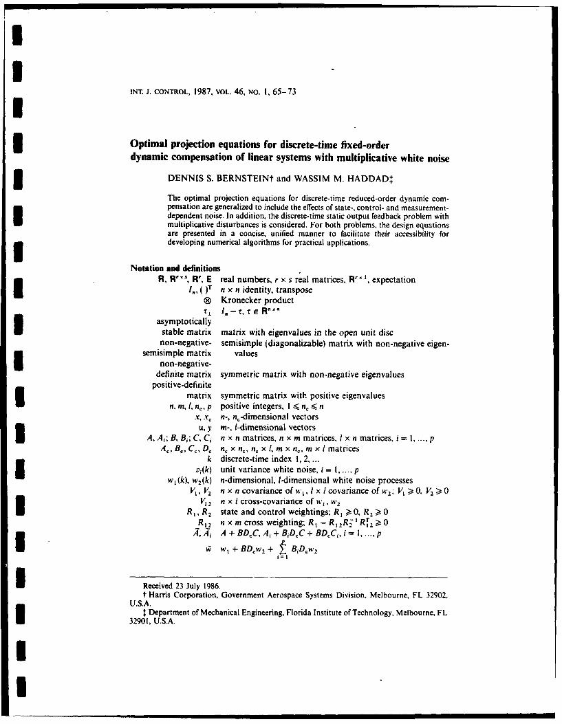
I3

INT. J. CONTROL, 1987, VOL. 46, NO. 1, 65-73I3Optimal projection equations for discrete-time fixed-order

dynamic compensation of linear systems with multiplicative white noise

3 DENNIS S. BERNSTEINt and WASSIM M. HADDAD++

The optimal projection equations for discrete-time reduced-order dynamic com-pensation are generalized to include the effects of state-, control- and measurement-dependent noise. In addition, the discrete-time static output feedback problem withmultiplicative disturbances is considered. For both problems, the design equationsare presented in a concise, unified manner to facilitate their accessibility for

*developing numerical algorithms for practical applications.

Notation and definitionsR, R'" , R', E real numbers, r x s real matrices, R'" ', expectation

,() n x n identity, transpose® Kronecker product

I. I,-r, T E..asymptotically

stable matrix matrix with eigenvalues in the open unit discnon-negative- semisimple (diagonalizable) matrix with non-negative eigen-

semisimple matrix valuesnon-negative-

definite matrix symmetric matrix with non-negative eigenvaluespositive-definite

matrix symmetric matrix with positive eigenvaluesn, m, I, no, p positive integers, I < nc < n

x, x, n-, nc-dimensional vectorsu, y in-, I-dimensional vectors

A, A,; B, B,; C, C, n x n matrices, n x m matrices, I x n matrices, i = 1. pAc, B,, Cc, Dc nc x n , nc x I, m x n, m x I matrices

k discrete-time index 1, 2, ...v,(k) unit variance white noise, i = 1 ... , p

w,(k), w2(k) n-dimensional, I-dimensional white noise processesV, ,Vz n x n covariance of w1, I x I covariance of w2; V, > 0, V2 > 0

V,2 n x I cross-covariance of w1 , W2

R1, R 2 state and control weightings; R, > 0, R2 >0R12 n x m cross weighting; R1 - RI 2R2' Rrt2 >04, 4i A + BDcC, Ai + BiDcC + BDCi, i = 1L..... p

v w, + BDcw 2 + BiDer,'2

IReceived 23 July 1986.t Harris Corporation, Government Aerospace Systems Division, Melbourne, FL 32902,

U.S.A.: Department of Mechanical Engineering, Florida Institute of Technology, Melbourne, FL

32901, U.S.A.

IU

I66 D. S. Bernstein and W. M. Haddad

V, +V1 2 DT B T + BDV + + BD V2D2T

1=1

Ri + RzDC + CTDT R12 + CTDR 2DcC + CTD R2 DcC

F J BC1 Fi. BiCl

AA, LBCC A' JL2i i

B,, + B, VO D " TV B T IR12C + CT DcR 2C.

C TRI2 + cT RC2R 2CD, ]ZOJ) (i,j) element of matrix Ztr Z trace of square matrix Zp(Z) rank of matrix Z I

Ei matrix with unity in the (i, i) position and zeros elsewhereni) qlEio-' (unit-rank eigenprojection)

For arbitrary n x n Q, P, ,. r define:

v, Vz+CQCT + CQC. R,A4R,+BTPB+ y BTPBi

=' i=l

Q5 =AQCr+V 1 2 + AiQC T, PABTPA+R1,+ BTPA,

Q5 4V 12 + A, P',, R2+ IZ BPA,

t~42 +CQCT+ Ci(Q + QTT Ri2 2 +BTPB+ BT(P + P)Bi

Q 3 4AQ12 +~2 p

A +rQr)C, A BTR 12 T

V,2 + i , P R 2 + T(P + ,P)A,

I. IntroductionHyland and Bernstein (1984) showed that the first-order necessary conditions for

quadratically optimal continuous-time fixed-order dynamic compensation can betransformed into a coupled system of four matrix equations (two modified Riccatiequations and two modified Lyapunov equations). The coupling is due to the presenceof an oblique projection (idempotent matrix) which arises as a rigorous consequence I

III

Optimal projection equations for dynamic compensation 67

I of optimality. This formulation provides a generalization of classical LQG controltheory, since in the full-order case the projection becomes the identity matrix, themodified Lyapunov equations drop out, and the modified Riccati equations reduce tothe usual LQG equations. Coupling via the optimal projection implies that sequentialreduced-order design procedures consisting of either model reduction followed bycontroller design or controller design followed by controller reduction are generallysuboptimal. Furthermore, the coupled structure of the equations yields the insightthat in the reduced-order case there is no longer separation between the operations ofstate estimation and state-estimate feedback, i.e. the certainty equivalence principlebreaks down.I The above developments for the continuous-time problem have, moreover, beencarried out by Bernstein, Davis and Hyland (1986) in a discrete-time setting. As in thecontinuous-time case, the optimal reduced-order compensator is characterized by apair of modified Riccati equations and a pair of modified Lyapunov equationscoupled by an oblique projection. Furthermore, because of the discrete-time setting itis now possible to permit static feedthrough gains in both the full- and reduced-ordercontroller designs. As pointed out by Hyland and Bernstein (1984). non-singularcontrol weighting and measurement noise in the continuous-time case permit only apurely dynamic (strictly proper) controller. Note that this is precisely the case incontinuous-time LQG theory, which yields strictly proper feedback controllers.

An immediate application of the discrete-time results is a rigorous treatment of thelinear-quadratic sampled-data reduced-order dynamic-compensation problem (Bern-stein, Davis and Greeley 1986). By explicitly accounting for real-time computationaldelay in the feedback loop, the sampled-data control-design problem can betransformed into an equivalent discrete-time problem. The dimension of the equiva-lent discrete-time system, however, is augmented by the available measurementswhich are treated as delay states. The optimal projection equations for discrete-timefixed-order dynamic compensation can thus be used to obtain controllers of tractablylow dimension in spite of dimension augmentation.

Design considerations concerning stability and performance robustness withrespect to unknown parameter variations can also be incorporated into the fixed-order dynamic-compensation design process. This can be accomplished by introduc-ing white noise into the plant via the imperfectly known parameters (Bernstein andHyland 1985, Bernstein and Greeley 1986 a). Intuitively speaking, the quadraticallyoptimal feedback controller designed in the presence of such disturbances isautomatically desensitized to actual parameter variations. As shown by Bernstein andGreeley (1986 b), the modification of the closed-loop covariance equation due tomultiplicative noise can be used to guarantee robust stability and performance bymeans of a Lyapunov function and a performance bound.

An interesting aspect of the design equations for the multiplicative noise model isthe breakdown of the separation principle even in the full-order case. That is, evenwhen coupling due to the oblique projection is absent, coupling due to stochasticeffects remains. This is a graphic portrayal of observations made previously, e.g. byGustafson and Speyer (1975). An alternative, apparently suboptimal approachinvolving certainty equivalent controllers for guaranteeing stochastic stability wasdeveloped by Yaz (1986).

The purpose of the present paper is to extend the optimal projection equations forfixed-order discrete-time dynamic compensation given by Bernstein, Davis andHyland (1986) to include the effects of state-, control- and measurement-dependent

II

68 D. S. Bernstein and W. M. Haddad Iwhite noise. The main result (Theorem 3.1) presents the necessary conditions foroptimality as a system of four matrix equations (two modified discrete-time Riccatiequations and two modified discrete-time Lyapunov equations) coupled by both theoptimal projection and stochastic effects. For the sake of completeness, the optimalityconditions for discrete-time static output feedback are given by Theorem 2.1.

2. Static output feedback2.1. Discrete-time static output-feedback problem I

Given the controlled system

x(k + 1) = (A + if vi(k)Ai )x(k) + (B + if vi(k)Bi)u(k) + w ,(k) (I)

yk=(C + vi vk)Ci x(k) + W2 (k) (2)I

where k = 1, 2, ..., determine D, such that the static output feedback law

u(k) = D,(k) (3) 3minimizes the performance criterion

JA lim E[x'(k)Rlx(k) + 2xT(k)R1 2u(k) + uT(k)R 2u(k)] (4)k - X U

Using the notation given at the beginning of this paper, the closed-loop system(1)-(3) can be written as

x(k +1)(A + Vit(k)A 1 )x(k) -- i(k) (5)

Define the second-moment matrix 3Q(k) = E[x(k)x (k)] (6)

satisfyingQ(k + 1) = AQ(k)%4T + A A1 Q(ki + V (7)

To consider the steady state, we restrict our consideration to the set of second-momentstabilizing gains I

S A {Dc: ,A® , + =Ai A, is asymptotically stable} 3The requirement D, e S implies the existence of the steady-state closed-loop statecovariance Q A lim Q(k). Furthermore, Q and its non-negative-definite dual P are

unique solutions of the modified discrete-time Lyapunov equations

Q = 4Tr + Ai /IQT: +" r(8) i

P=-p, PA+ 41Y ,P, +/) (9)

lI

Optimal projection equations for dynamic compensation 69

3 An additional technical requirement is that D, be confined to the set

S*A{DeS:V 2,>0 and R 2,>0}

In order to obtain closed-form expressions for extremal values of the closed-loopcontrol gains, the static- and dynamic-compensation problems require the technicalassumption3 [Bi# 0=.Ci=0], i=1,..., p (10)

i.e. for each ie {l.p}, B, and C, are not both non-zero. Essentially, (10) expressesthe condition that the control-dependent and measurement-dependent noises areindependent. There are no constraints, however, on correlation with the state-dependent noise. By optimizing (4) with respect to D, and manipulating (8) and (9), weobtain the following result.

I Theorem 2.1

Suppose D, e S + solves the discrete-time static output-feedback problem. Thenthere exist n x n Q. P > 0 such that

_ R - IR[BT PAQCT + PQCT +BTpQi] V" (1)

and such that Q and P satisfy

Q =AQA T + V, + [(Ai + BiDcC)Q(A, + BiDcC)T + BiDV 2D BT]V2.BTDVQD' B Q]

3 + (Q + BD.V 2 .) V2 '(Qs + BDcVZ,)T - QVQT (12)

PATpA + R, + [(Ai + BD 5 JT P(Ai + BDcCi) + CTDIR 2D5C1 ]

+ (P, + RZSDC)TR2SI(P, + R2,D C)- P RZSP, (13)

3. Dynamic output feedbackWe now expand the formulation of the static problem to include a dynamic

compensator.

3 3.1. Discrete-time dynamic output-feedback problem

Given the controlled system (1). (2), determine A,, B,, C,, D, such that the dynamicoutput-feedback law3 x(k + 1) = Ax,(k) + B,(k) (14)

u(k) = C~x.(k) + Dcifk) (15)

minimizes the performance criterion (4).

We restrict our attention to the second-moment-stabilizing controllers

A> {(A,. B,, C,. DC):,® + ,® is asymptotically stable and

(rA,, B,,) is minimal}

which implies the existence of A lim E[.(k).Tr(k)], where R(k) A [XT(k), XT(k)] T .I -

I-U unmnIam l lm lI l nll l l n • nl

II

70 D. S. Bernstein and W. M. Haddad

Furthermore, 0 and its non-negative-definite dual P are the unique solutions to the Umodified discrete-time Lyapu..ov equations

Q=AQA ' j A 1 A[+ r (16)I

+ A (17)

An additional technical assumption is that (Ac, B,, C,, D ) be confined to the set

+A- {(A¢,B ,CD,) ES:I9,,>0 and V?, >0,1

The following lemma is required.

Lemma 3.1 3Let r - F"'R. Then

T2 r (18) 3p(r) =n. (19)

if and only if there exist G, F E R".." such that

GT F = r (20) IrGT = 1., (21)

Proof ISee Bernstein, Davis and Hyland (1986).

For convenience call G and F satisfying (20) and (21) a proiectire factorization ofr. IFurthermore, for n x n non-negative-definite matrices 0, P. define the set of contragre-diently diagonali:ing transformations (see Rao and Mitra 1971. p. 123)

D(Q, i). ep c R" m: q-,-I&-T and OT 0, are diagonal'

Theorem 3.1Suppose (A,, B,, C¢, Dj E S solves the discrete-time dynamic output-feedback

problem. Then there exist n x n Q, P, Q. 5 > 0 such that

A,= A- B s' 5 - .V-' C - BDC]G T (22) 3B, = F[Q"2, + BD,] (23)

C, = -[I' P, + DC]GT (24) 3D,= -/2-s[BTPAQCT+P/5 QCT+BTP0,.1ff",; l (25)

and such that Q, P, Q., P satisfy 3Q = AQAT + V, + rQT + [(.4, - BI, 1' P,)5 rT (A - Bi-'L P )1T

+(A, + BDC)Q(A, + BiDC BjDV, BT] - O.f/,-I (26)

II

II

Optimal projection equations for dynamic compensation 71

P AT pA+R TP,+ [A T rT 15( "-1 ICi

+ (Ai + BDCI)TP(A, + BDC) + CTD RZDC ] - PsTR- Ps. (27)

Q (A - B9s P5p)TQtT(A - BR2,I 15,)T + (Q, + BD, 2 (Q, + BD, V2)T (28)Q=(A -- I C)TtTP"(A - Q3 V ;C)+( 5 + R 25DcC)TA 3-II5 + A 2, DC) (29)

where

t A fi( )=GTF (30)

for some 0 e D(Q, P) such that (0 -I 0P0q)(,. # 0, i = I. n, and some projective3 factorization G, F of t.

Remark 3.1To specialize the result to the strictly proper (no feedthrough) case, merely ignore

(25) and set D, = 0 wherever it appears.

Remark 3.2As previously pointed out by Bernstein. Davis and Hyland (1986). the indeter-

minacy in specifying the projective factorization G, F satisfying (20) and (21)corresponds to an arbitrary choice of internal state-space basis for the design system(A, B,, .

Remark 3.3In the full-order case n, = n, the projection T becomes the identity and (28) and (29)

play no role. In this case GTF = rGT = 1. and thus G and F can be chosen to be theidentity. Deleting all multiplicative white noise terms corresponding to state-, control-and measurement-dependent disturbances, i.e. Ai, BI,. Ci = 0. i = I. p, and specializ-ing further to the purely dynamic case (D. = 0) yields the standard LQG result.Alternatively, setting n, < n and deleting the multiplicative noise terms yields the3 Iresults of Bernstein, Davis and Hyland (1986).

4. Proof of Theorem 3.13 Partition (n + n,) x (n + n,) (, into n x n. n x n, and n, x n, sub-blocks as

1T2 Q2 12 pT ,

I and define the n x n non-negative-definite matrices

IQAQ 1 Q1 2 Q tQI2 . PP, -P 2P2'P 23 QQIQ T j

3p-p

T

OA (A - BA J ^,)(A - BRA' P,)T +(0' + + B);'(, )

P5A (A - .- C)T AA - -C) + (P5 + R23K),( t (R2 1P 5 + RZ2,DC)

where T ,T and rTPt" in Qs, fl, P2 ,. and 'i2, are replaced by Q and P, and the n, x n,InI

II

72 D. S. Bernstein and W. M. Haddad

n, x n, and n, x n matrices IGA~QI12, M=Q 2P2 , r =-P PI2

Define the lagrangian

L~AC B~,CD~, )-Atr [AJ(A,, B,, C, D,) + (A~ + A, -QP

where the Lagrange multipliers . > 0 and P c- + n ) (n +n ' are not both zero. Setting IaL/ Qa=0, . =0 implies P =0 since (Ac, Be, Co, D) E S+. Hence, without loss ofgenerality, set = 1. Thus the stationarity conditions are given by

L =I A T+ l oT + 0 (31)~i= I

TL =*,%P + TP= + A -,P (32)cQ

A,= P12AQ1 2 + pJ2 BDCQ1 2 + PJ2 BCCQ 2 + P2A Q2 + P2 BCCQ, 2 =0 (33) 3B= P2B ,+ f12 0 + P1 2 BD, ,= 0 (34)

CL = P5sQ 12 + RsCcQ2 + R 2SDCCQI 2 =0 (35)

cL = R2 sDcV 2, + BTpAQCT + P1,QCT + BTpQ, = 0 (36) 3eD,

Expanding (31) and (32) yieldsAQA T + (Q, + BD1 2 3)-,; '(Q3 + BD 0,/) - IT

+ (A - BfiD'13)Q(A - B-IC j5)T

+(,+B1 ~)(A ~DCT+BIDe V2 Dc Bi] = 0 (37),+ BD ,)f- '(Q, + B[(A23 ,) +(A - B;,' P5) (A - BRA P' - Q]r T = 0 I

(38)l"T(Q, + BD 2 , ) 1 ; '(Q, + BD, + 2)

T

+ (A - BRs2 'f.P)Q(A - Bs.I P) T - Q]r = 0 (39)

ATPA + (P, + A2 ,DC)TRI2s,1 (06 +A 2,DC)- 6r; 2' PI

+(A - ',V 2 C)T (A - ,P2; 'C)+ R, - P - P +,, [(A,-i I ,C,)TP(Aj,- .,P2,-I C,)I

+(Ai + BDCi)TP(A, + BDCi) + CTDR 2 DCC] 0ICi D ,Ci=O (40)

UP, + 92,DcC)T i -I (f, , + A2,,DC) + (A I C)T A - 0,1V;'C)- P]G T =0 3(41)

II

Optimal projection equations for dynamic compensation 73

G[(P3 + t 2 3OcC) T ?(P23 R92,5DC) + (A - A(C)TA - Q., -P =C)~(42)

Using (33)-(36) we obtain (22)-(25). Using (37) + GTr(38)G - (38)G - (38G)T andGTr(38)G - (38)G - (38G)T yields (26) and (28). Similarly, using (40) + r TG(41)rS(41)r- (41r)T and rTG(41)F-(41)r-(41F)T we obtain (27) and (29). Also,F(38) - (39)_or G(41) -(42) yields FGT = Ino so that r = G Tr r'. Finally. (39) and(42) imply Q = TQrT and 6 = zTTr.

Remark 4.1An interesting differer;..- between the above discrete-time derivation and the

continuous-time derivation of Hyland and Bernstein (1984) is that the explicit gainexpressions and the definition of the optimal projection arise in the reverse order.

5. Directions for further researchThe principal application of Theorems 2.1 and 3.1 is the sampled-data problem with

parameter uncertainties. Although generalization of the results of Bernstein et at.(1986) is possible, there appear to be a number of mathematical issues whicharise. A related development appears in Tiedemann and De Koning (1984). A moreextensive treatment of the results of the present paper can be found in Haddad (1987).

ACKNOWLEDGMENTDr. Bernstein was supported in part by the Air Force Office of Scientific Research

under contract AFOSR F49620-86-C-0002.

I REFERENCESBERNSTEIN, D. S., DAVIS. L. D., and GREELEY, S. W., 1986, I.E.E.E. Trans. autom. Control, 31, 859.BERNSTEIN, D. S., DAvis, L. D., and HYLAND, D. C., 1986. J. Guid. Control Dynam., 9, 288.BERNSTEIN, D. S., and GREELEY, S. W., 1986 a, I.E.E.E. Trans. autom. Control. 31, 362; 1986 b.

Proc. American Control Conf.. Seattle, WA, pp. 1818-1826.BERNSTEIN, D. S., and HYLAND, D. C., 1985, Proc. 24th I.E.E.E. Conf. on Decision and Control,

Fort Lauderdale, FL, pp. 745-752.GUSTAFSON. D. E., and SPEYER, J. L., 1975, J. Spacecraft Rockets, 12, 351.HADDAD, W. M., 1987, Robust optimal projection control-system synthesis. Ph.D. dissertation.

Department of Mechanical Engineering, Florida Institute of Technology.HYLAND. D. C., and BERNSTEIN, D. S., 1984, I.E.E.E. Trans. awtom. Control, 29, 1034.RAO, C. R., and MITRA, S. K., 1971. Generalized Inverse of* Matrices and Its Applications (New

York: Wiley).TIEDEMANN, A. R., and DE KONING, W. L., 1984, Int. J. Control. 70, 449.YAZ, E., 1986, I.E.E.E. Trans. autom. Control, 31, 586.

IIII

ISIAM J. MATRIX ANAL. APPL. 0 1988 Somly for industra and Appled Maihea iv-Vol. 9. No 2. Apni 1988 002

IINEQUALITIES FOR THE TRACE OF MATRIX EXPONENTIALS*

DENNIS S. BERNSTEINt

Abstrc. Several inequalities involving the trace of matrix exponentials are derived. The Golden-Thomponinequality tr e* 8 ; tr e' s for symmetric .I and B is obtained as a special case along with the new inequallttr i tKr t,' " for nonnormal .4.

Ke) words. matrix exponential. inequalit., trace

AN.S(MOS) subject classification. 15

I. Introduction. For n , n real symmetric matrices .-I and B. the Golden-Thompsoninequali(\ [I]-[5 states that

(1.1) Ir I' =< itr I, ',.

Reference 15] generalizes (I ) to allow arbitrary spectral functions in place of the traceoperator and provides an o\ersiew of applications in which these inequalities arise.

In contrast to ( 1. 1 ). problems in linear-quadratic optimal fieedback control [6] typ-icall. involve a performance functional J of the form

3 (1.2) J =tr (,'-tI'v,4c"R di.

where I and R denote noise intensity and performance weighting matrices. respectively.and A denotes the linear system dynamics matrix. The form of (1.2) thus suggests in-equalities of the form (1.1) involving A and .41. where A is nonnormal. in place ofsymmetric .4 and B. Such inequalities are motivated b\ robust sampled-data control-design problems which require performance bounds for uncertain s\stem models.

The main result of the present note is the inequalit%I I - " Ii • -

(1.3) tr "'v = tr I'

Rather surprisingl\. the sign of the inequalit. (I.3) i,, oppositc to the sign of (1.1). Tounderstand %hN this is the cas,. we dcri c a series ofinequaliti-s which, upon appropriatespecialization. yield both ( 1. i) and (1.3).

2. Inequalities. Thi- I'ollo\ ing lemma is required. (Let C ' denote the transpose ofa matrix ('.)

LIi Mi.\ 2 1 R' and t id u 0 lP,)klu 1' /III( L!('?. t/('11

(2.1I ) tr ( tr "( '' tr (('K,.

Pro,, 'lic first inequalht tolloas fromn tr W" - (") ( '' - ( ) O. 'hile thesecond flo s from a resuh of K. Fan (ek [4. pp. 234. 516]). D

i f 0RI \t 2.1. It.1. B E R' .lt,tr I, " . = l r c, - ' t, i •tlt _. r ,

'f 1

! • I ¢ ).1 2.2c Ir =.t t

t r I , .1.,,

/

(2.3) 219) :5 tr (v ",," + el'efl)- , tr We " A + ," B -II).tr r + -'

Received h the editors Januar\ 21. I'4?t7: accepted for publication Ma. It. 1987 This research wassuppo~rted in part b,, the Air Force Office of'Scientific Research under contract F4Y620-fi0-C'-XK)2.t Harris Corporation. Melbourne., Flonda 32902

156

U

IU

INEQUALITIES FOR MATRIX EXPONENTIALS 157

Proof Defining C = e'1B/2' (2. 1) becomes Itr (eA/ 2re B 2r) 2r -< tr (c4f2re f2")(er/z1reA T/2r)r 5 tr (eAIe2reB12reftT1/re.4Tr)r

.

Letting r - o-_, the exponential product formula 15, p. 60] and its generalization[7. p. 97) yield the first two inequalities of (2.2). The third inequality of (2.2) followsfrom Corollary 3 of [5] while the fourth inequality of(2.2) follows from

0 =5 tr [((.4 . A7)12 - e(B + Br)/' ] .

To prove (2.3) note that the upper leftmost inequality follows from 0 Str (e- - e8 )(' - e)7. The remaining inequalities in (2.3) follow from tr etr e4e4t 6 tr e 4 . which is a consequence of(2.2) with B = .4. El

COROLLARY 2. 1. /1 E R' " ", then

(2.4) . 4 - ' < n(2.4) ~ ~~ ~ ~~~ tre- - re re' - + 2 tr e' (4 - 4 1),

24<n 1 ".4 " n 1 '(4- 4 r

(2.5) tre-ee"5 tre e --7 te- " . I2 2 2 2te

If A, B E R"' " are symnetric, then

(2.6) tr e 4 8<_ tr eAe B g tr (e24 + e-B).

Proof The first two inequalities of (2.4) follow from the first two inequalities of(2.2) with B = A. The last inequality of(2.4) follows from the last inequality of(2.2) withB = 0 and A replaced by 2.4. Inequalities (2.5) follow from (2.3) with B = 0 and Areplaced by 2.4 while ignoring the lower leftmost term in (2.3). Finally. (2.6) followsfrom (2.2). El

Remark. The second inequality in (2.4) and the first inequality in (2.6) correspond* to (1.3) and ( .1). respectively.

3. Additional inequalities. I he question immediatel. arises as to whether an% ad-ditional inequalities in~olving the expressions appearing in (2.4) and (2.5) arc true. Notethat tr C'iC'I in (2.3) cannot be merged with (2.2) because of the sign resersal between(1.1 ) and (1.3). It can readil. be seen that the onl. remaining possibilities are

(3.1) tr J tr I(3.2) tr ." 1 f , :c, tr (,'- 1+.

(3.3) tr c.'t tr (c

B\ randomly generating ..1 and B. (3.1 ) was shon to be false. Since (3.2) implies (3.11.(3.-2) must also be false. Furthermore, in the case B' -B. inequalitN (3.1 ). whichbecomes

(3.4) tre 4 4'41 2, 1 tr+ Ir c't 4

was also shown to be false. Hence (2.4) and (2.5) cannot be merged. Finally. the remaininginequality (3.3) was also shown to be false even when B = 0.

Remark. The results of this paper can be generalized to the case in which A and Bare complex matrices. Generalization to arbitrary spectral functions [5] remains an areafor further research. I

I

II

158 DENNIS S. BERNSTEIN

I Acknowledgment. I wish to thank Scott W. Greeley for carrying out numericalcalculations which suggested the results of this paper.I

REFERENCES

11) S. GOLDEN, Lower hounds.for tie He/mholt: function. Phys. Rev.. 137 (1965). pp. BI 127-B 1128.12) C. J. THOMPSON. lnteiialit" with applications in statistical rmchani.s, J. Math. Phys.. 6 (1965). pp. 18 12-

1813.

[3] A. LENARD. Generalization oftthe Golden-Thompson Inequality Tr (eAeo) ? Tr c' ''. Indiana Univ. MathJ.. 21 (1971). pp. 457-467.

[4] A. W. MARSHALL 'ND I. OLKIN. lnequalitic.: TheorY of.Aajorization and lto .4pplication. Academic Pres.New York. 1979.

151 J. E. COHEN. S. FRIEDLAND. T. KATO. AND F. P. KELLY, Eigenvaliu inequahliei fir products of Pnatri\

exponmitals. Linear Algebra Appl.. 45 ('1982). pp. 55-95.[6) K. KWAKERNA#,K AND R. Svo kN. Linear Optimal Control Systems. John Wiley, New York, 1972.[71 V. S. VARADARAJAN. Lie Groups. Lie .4gebras. and Their Representations. Springer-Verlag. Berlin. Nc%

York. Heidelberg. 1984.I

IIIIII

II

I|

I I

I SIAM RmvEt 0 1988 Soceely fror Indlustril and Applied Ma~Meatic"s

Val. 30. No. 1. Mamb" 0988 006

PROBLEMS AND SOLUTIONS

EDITED BV MURRAY S. KLAMKINCOLLABORATING EDITORS: CECIL C. ROUSSEAU OTTO G. RUEHR

All problem. and solutions should be sent, tIpewriten in duplicate, to Murrav S. Klamkin, Departmentof Mathematics; University ofAlberta, Edmonton. Alberta. Canada T6G 2G I. An asterisk placed beside aproblem number indicates thai the problem was submitted without solution. Proposers and solvers whosesolutions are published will receive 5 reprints ofthe corresponding problem section. Orher solvers will receivejust one reprint provided a self-addressed stamped (U.S.A. or Canada) envelope is enclosed. Propaser andsolvers desiring acknowledinrent of their contributionsshuld include a self-addressed stamped postcard(no stamps necessary outside the U.S.A. and Canada). Solutions should be received bh' June 30, 1988.

PROBLEMS

Commuting Matrix Exponentials

Problem 88-1", by DENNIS S. BERNSTEIN (Harris Corporation, Melbourne, Florida).In feedback control theory for sampled-data systems, the equivalent discrete-time

dynamics matrix is given by eAh, where h is the sample interval and A is the dynamicsmatrix for the original continuous-time system. When A is perturbed by Ao (duepossibly to some modeling uncertainty), then it is necessary to consider e(I A'O . Forrobust control system design it thus may be of interest to know when e("4)' can bedecomposed into a nominal part involving A and a perturbed part involving Ao.Analogous questions arise in the study of bilinear control systems of the form

x = Ax + uBx,

where u is a scalar control. In this case the Lie group generated by A and B plays acentral role. Again, it is of interest to know how e-"' is related to e' and e'. theprincipal result being the Baker-Campbell-Hausdorff formula. Of course, it is wellknown that when

(I) AB= BA,

where A, B are real n x n matrices, then both

(2) e~ t e

and(3) v''= +

hold. It is less well known that the converse is not true. Specifically, examples aregiven in [I] which show that (2) may hold while (1) and (3) are violated, and that (3)may hold while (1) is violated. Interestingly, it is stated without proof in [I] that

(3) implies (2). Prove this claim or find a counterexample. A copy of [I] is availablefrom the proposer.

REFERENCE

(I I M. FREcHET, Les solutions non commutables de I'equation matricielle ee' - elr- , Rend. Circ. Mat.Palermo 2, (1952), pp. 11-27.

123II

II

IROBUST STABILITY FOR SAMPLED-DATA CONTROL SYSTEMS I

Iby I

Dennis S. Bernstein C.V. HollotHarris Corporation Department of ElectricalGovernment Aerospace Systems Division and Computer Engineering

MS 22/4848 University of MassachusettsMelbourne, FL 32902 Amherst, MA 01003

UABSTRACT 3

In this paper we consider the robust stability of a continuous-timesystem under computer control. The uncertainty is modeled as additive per-turbations to the matrices in a continuous-time state space description ofthe plant. Our methods exploit the resulting exponential-like uncertaintystructure in the sampled-data control system and we develop sufficientconditions for such a system to be robustly stable. 3

IUIUII

III

1. Introduction

A sampled-data control system consists of a continuous-time plant under

computer control; see Figure 1. Generally speaking, if the matrices in a

state space description of a continuous-time plant are uncertain, then the

resulting closed-loop, discrete-time system possesses an exponential-like

uncertainty structure. This is true even if the continuous-time plant has

linear uncertainty. Existing methods; e.g., see [1]-[41, are inadequate in

analyzing such uncertain discrete-time systems since they do not directly

handle these exponential-like structures. Notable exceptions include the

conic sector approach in [51, and the stochastic parameter formulation in

[6]. Indeed, the present paper was motivated by the approach of 161 which,

as shown in [121 can be reinterpreted to yield conditions for deterministic

robust stability. Our objective is thus to develop a robust stability test

which exploits the specific nonlinear uncertainty structures occurring in

sampled-data control systems.

In the sequel, the following notation will be used. For X e Rn xn , X,

denotes the transpose of X, while X > 0 (X > 0) means that X is positive

definite (positive semi-definite). The spectral radius of X is given by

p(X). Lett-,Gand "vec" denote the Kronecker product, Kronecker sum and

column stacking operators respectively; see [9]. In addition we shall use

"vec- 1" to denote the operation of forming a (usually square) matrix from a

column vector.

* 2. Problem Formulation

In this section we state the robust analysis problem for sampled-data.

control systems using static feedback. To begin, consider the n-dimensional

continuous-time plant

3 *(t) = (A + 6A)x(t) + (B + AB)u(t)

y(t) = Cx(t)

where A c Rnxn , B c Rn ' and C C R xn denote nominal state space data and

where A and AB represent perturbations in A and B respectively. The pair

I

I

21

of suitably dimensioned matrices (&A, AB) belongs to an uncertainty set U Igiven by

p p p 2U =((A, AB): AA = E a.A. and 6B = E .B., a. < 1}i=l i=i =l 1 - ( .

(2.1) Iwhere A. and B. reflect the "structure" of the uncertainty and where a. is1 1 1

an uncertain real parameter; note that an uncertain parameter a. may appear1I

in both A and AB, and it's possible to have A.= 0 and B. * 0 or vice-versa.I 1

Now, consider the sampled-data system in Figure 1 with a sampling

period of h seconds. We assume perfect synchronization between the A/D

(sampler) and the (D/A) (zero-order hold) and ignore finite word-length

effects and computational delays. We also assume that a static control law

u(kh) - Ky(kh); k = 0,1,2,..., 3(2.2)

is implemented for some given gain K . Rm x

Our purpose is to analyze the robust stability of this closed-loop

system, and to this end we consider its evolution at the sample instances kh

by forming the associated discrete-time system 3x(k+) =[e(A + A)h +- e(A + MA)t dT(B + AB)KClx(k).

0(2.3)

In the above x(k) denotes x(kh); we have abused notation for the sake of 3conciseness. Given arbitrary (AA, AB) c U, system (2.3) is discrete-time

stable if all the eigenvalues of

e (A + M)h + e(A + AA)Tdr(B + AB)KC0

lie within the open unit disk. Additionally, (2.3) is said to be robustly

discrete-time stable if it is discrete-time stable for all (A, AB) c U.

3. Main Result i

I

I 3.

I We nov develop a sufficient condition for the robust stability of

(2.3). This condition exploits the exponential structure of the uncer-

tainty; i.e., rather than "overbounding" the uncertainty with an additive

model of the form

x(k+l) = (i + 61)x(k),

our methods treat the exponential structure of the nonlinearity in (2.3)

more directly.

To show robust stability we will construct a parameter-independent

(independent of the uncertain matrices (A, AB)) quadratic Lyapunov function

V(x) for (2.3). Thus, let P be some free, positive-definite symmetric

matrix and consider the quadratic Lyapunov candidate

V(x) = x'Px, x Rn.

System (2.3) is robustly discrete-time stable if

IV(A, AB, P) =

d[e(A)KC+ eAA~Ahh + (A+)'S(A+AA)h + e( d T(B+AB)KC P [e ( A+ A) h + e(A+AA)d(B+AB)KC] - P

(3.1)

is negative definite for all (A, AB) c U. This follows since x'1Vx is the

Lyapunov difference associated with V=x'Px and (2.3); i.e.,

x'AV(AA, AB, P)x = V(x(k+l)) - V(x(k)).

System (2.3) is robustly discrete-time stable if this difference is negativefor all x c Rn and all (AA, AB) c U; e.g., see [7].

A critical step in our development is to express the uncertainty in

(3.1) solely in terms of the matrix exponential. Indeed, using the identity

(see [8])

I

II

4I

exp( (A + A) (B + AB) h) e(A+M)h e) dT(B+AB)

(3.2)

(3.1) can be rewritten

AV(AA, AB, P) =1

[I O]exp( [(A+ AA) (B+B)]h) [ I ]P[j C'K' ]exp( [(A+MA) (B+AB)]'h)[ ] IP(3.3)

Our next result provides a parameter-independent upper bound to AV. To give Ithis bound, let o > o be given and define

[A B , , [ B] + + I+! Bi]®2)[Ai Bj]

i~l (3.4)Iand

= C ]P [I C'K'1l

(3.5)Lemma 3.1 (See Appendix for proof): If P c R positive definite

and symmetric and > 0, then

AV(MA, AB, P) =

[I Olexp([(A 'A (B+AB)]h) [I ]P[I C'IKjexp( (A MA) (B+B ih) i001 KC I100 0I

< [I 01 vec-1 [e vec(Hp)][0 - P

(3.6)

for all (A, AB) c U. VVV

Now, using the right-hand side of (3.6), formally set

I

II

i5

[i 0] vec-[e cc vec(IH)][0 - P = -IS(3.7)

which is equivalent to

(M- I)vec(P) = -vec(I)

(3.8)

i where

M [I 0]e ' h KC KC

(3.9)3 When does (3.8) have a positive-definite solution? Our next lemma gives a

sufficient condition.

i Lemma 3.2 (See Appendix for proof): If there exists an o > 0 such that

p(M) < 1,

(3.10)

then (3.8) has a positive-definite solution P. VVV

Now, assume (3.10) holds for some a > 0. From Lemma 3.2, equation

(3.7) has a positive-definite solution P; hence, using (3.6) and (3.7) it

follows thatI_AV(AA, AB, P) < -I -

I (3.11)

for all (MA, AB) s U. We have thus proven the following main result.

i Theorem 3.1: If there exists an c > 0 such that

p(M) < 1,

3 then the sampled-data system (2.3) is robustly discrete-time stable.

I

II

6I

It's important to note that the condition of Theorem 3.1, p(M ) < 1, is Ialways satisfied if the "nominal" system is stable and there is no uncer-

tainty; i.e., A = 0 and AB = 0. Indeed, taking c = 0, a straightforward

manipulation using (3.2), (3.4), (3.9) and identities (A.1) - (A.4) in the

Appendix gives

S= (e Ah + f eAxBKCdr)®(eAh + e ABKCd T).

(3.12)

Since the nominal system is stable, then all the eigenvalues of I

eAh + f0 eA BKCd r

lie within the unit disk. This implies, together with (3.12) and the fact Uthat the eigenvalues of a Kronecker product of two matrices are the products

of the eigenvalues of these two matrices (see [9]), that all the eigenvalues

of M lie within the unit disk. Thus, p(Mc) < 1.

The stability result of Theorem 3.1 is also valid for the case when

(2.3) has time-varying uncertain parameters ai(t). This is a consequence of

having established stability via a parameter-independent Lyapunov function.

Finally, we remark that a dual result holds when AB =0 and one allows uncer-

tainty in C; i.e, C 4 C + C.

4. Example IIn Soroka and Shaked [131, the robustness of a continuous-time system

under "cheap" LQ regulation is studied. The resulting closed-loop system is

described by

x(t) = [A + (B + AB)L rJx(t) I

y(t) = Cx(t)

(4.1)I

I

II

1 7

I where

AA = 0; AB = aB 1; 2 < 1; >

(4.2)

and where the LO regulator gains are given by

Lr = [1 + q - V3 + 2q 2/5+2q - q -41'; q= v4+(4 3

with r > 0 being the control weighting in the quadratic performance index

I Jo[Y2(t) + ru 2(t)]dt.

Soroka and Shaked showed that stability robustness decreased as the control

became more cheap (r 4 0).

Now, suppose this LO regulator gain is to be implemented in a computer.

What is the robustness of this sampled-data control system? We shall use

the sufficient condition in Theorem 3.1 to help answer this question.

First, however, we translate the continuous-time LQ gain to one suitable for

sampled-data control since the nominal discrete-time system is unstable if

we implement gain K = Lr in the computer. Following [pp. 189-191, Astrom

and Wittenmarki, we take

K = L 11 + (A - BL )h/21.(4.4)

For given sampling period h, control weighting r and uncertainty bound a, we

are now in a position to determine if p(M) < 1 for some c > 0. For ex-

ample, for h =.l, r = .05 and a = .5, we plot p(M ) versus a in Figure 2 and

observe that p(M) < 1 for a > .3. Hence, the sampled-data system is stable

for a = .5. Also, for h = .1 we determine, for various r, the largest a for

which p(M ) < 1 for some a > 0. We compare these results to the actual

I

I I I

8

discrete-time stability boundary and to Soroka and Shaked's results (13]; 1see Figure 3. To compute the the actual discrete-time stability boundary,

we assume time-invariant uncertainty aI and find the largest a for which

(4.5)

for all jalI < a. Recall that the stability result in Theorem 3.1 is valid

for time-varying uncertainties 1(t) as well; hence, it's natural to expect

that the resuts using p(M ) will be conservative compared to those using

(4.5). This was indeed true except for values 1/r = 10. For these values,

the stability criterion of Theorem 3.1 predicts ranges of stable a which

are larger than those computed using (4.5). This is clearly incorrect and

we contribute these discrepencies to roundoff errors in the computations.

Finally, we note that the actual discrete-time stability region is larger i

than its continuous-time counterpart. iACKNOWLEDGEMENT

We thank Mr. Mujdat Arabacioglu for his assistance in preparing the example. iIIiiII

II

I 9

APPENDIX: PROOF OF LEMMAS 3.1 AND 3.2

To prove Lemmas 3.1 and 3.2 we first need some identities and observa-

tions; see {q] for details.

I Identities: If X c Rr x r and Y c RSXS, then by definition the Kronecker

sum is given by

X®Y =.X®I + i Y.l (A.1)

Next, if the indicated products exist, then

I vec(XYZ) - (Z' O)X)vec(Y)

(A.2)

(X )Y)(ZDW) = (XZ) (D(YW).(A.3)

Finally, if X is square, then

eIX X = eX ®eX. (A.4)

Observation 1: Given arbitrary (6A, 6B) C U, the solution to the

* matrix differential equation

Y(t) = [(A+AA) (B+AB)]Y(t) + Y(t)[(Ao6A ) (B+oB)], t > 0, Y(O) =YO(A.5)

3 is

Y(t) = exp([(A+AA) (B+AB)]t) Y0 exp([(AM) (B+6B)]'t) (A6

This is a well-known result.

Observation 2: Let o > 0, then the solution to the matrix differential

3 equation

U

II

10I

Y(t) = ([ + I )Y(t) + Y(t)([ + 0 ) + ! Bi](t]

t_ O, ( =Y 0

(A.7)

is

Y(t) = vec-1 le tvec(Yo)J.

(A.8)

To show (A.8), apply the "vec" operation to both sides of (A.7) and use

identities (A.1) and (A.2) to get~I

vec(Y(t))=

p ([j~ Bi] or, B,)vc()

[IA B] o, (D( [A B] + a )+ 1 Z~ 0P4 ))e (A.)(A.9)

The solution to (A.9) is

Ktvec(Y(t)) =le vec(Y0o)]

from which (A.8) follows.

Observation 3: If c > 0 and if 70 is positive semi-definite, then the.solution in (A.8) satisfies

Y(t) =vec' [e vec(Y 0 )1 > 0, t > 0.I

(A.9)To prove this observation, let S,N c Rrxr with N positive semi-definite.

From (A.2)

- ""(S OS)vec(N) = vec(SNS')

I

II1

I vhich implies

vec [(S eS)vec(N)J = SNS' > 0.

(A.10)

3 Using (A.3)

(S®@S)i = (Si's

i)I. (A.l1)

so that

vec- [eS ® vec(N)] = vec [ Z (i!)-l(S(®S)'vec(N)IIi=O

= vec-1 £ (il)-(Si DSi)vec(N)JIi=O

I= Z vec-l11[(Si (si s)vec(N)]i=0

= Z (i! ) 1 S S)i=O

I > 0.

(A.12)

Furthermore, from (A.4) and (A.10)

vec- I[eS Svec(N)] = vec- [(e S e S)vec(N)I

= eSNeS '

>0.w u(A.13)

Now, using the exponential product formula (see [10, pg. 97]) we write

II

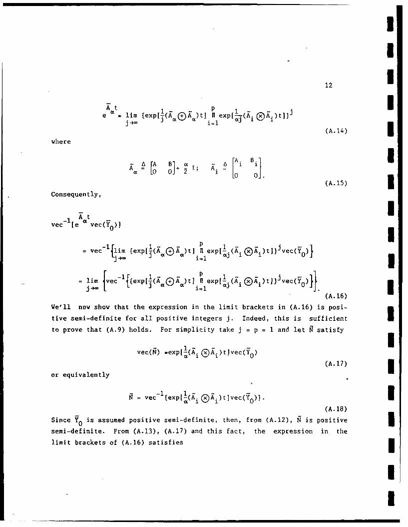
II

12

t p 1

e lim (exp[t(A ) Qt n1 expf_-(A(®)Ai) t]

(A.14)

where

A [A B]+ cc; A B ]* Ia= 0 + I 0.=

(A.15)

Consequently,

vec-1 [eAvec(Yo)J

vec -lim [exp[-(A QA)t I exp[-.(A.K DA)tJ) vec(Y0 )}

1-i~ I ~]~vcY

=lim ec- 1 (exp[!( A®(AK)tjil exp['-( i (D )tl i]vec(Yo)"(A.16) I

We'll now show that the expression in the limit brackets in (A.16) is posi-

tive semi-definite for all positive integers j. Indeed, this is sufficient

to prove that (A.9) holds. For simplicity take j = p = 1 and let N satisfy1 - ®Atvec(Yo)

vec(N) =exp[-(X(i )t](A.17) I

or equivalently

vec- 1 exp[1(AiAi)t]vec(70)}.

(A.18)

Since Y0 is assumed positive semi-definite, then, from (A.12), N is positive

semi-definite. From (A.13), (A.17) and this fact, the expression in the

limit brackets of (A.16) satisfies

II

II

I 11

3exp[(KAQAg)tlexp[(A. OA.,)tlvec(Y0 ) = exp[(A®AK)tvec(ff)

*~ >0.

A similar argument, using (A.12) and (A.13) alternately, shows that the

expression in the limit brackets of (A.16) is positive semi-definite for

arbitrary positive integers j and p. This completes the proof of

3 Observation 3.

Proof of Lemma 3.1: Assume P positive definite and c > 0. Furthermore,

consider the matrix differential equations in (A.5) and (A.7) with

y - - (A.19)

where HP is given in (3.5). Subtracting (A.5) and (A.7)-gives

3 Y(t)-Y(t) 0 [ (Y(t)-Y(t)) + (Y(t)-Y(t))[(A M) (B+0 0 Y

t > 0, (o)-Y(o) = 0

I (A.20)

where

I - pTI (t) = A~t + Y(t)A' + E A AY(t)AM3 ° i=l 1 1

([(A+ A) (B+AB)] (t)+ Y(t)[(A+A) (B+ B)]'(I vi ~ vi(A. 21)

and where A and A. are defined in (A.15).

Claim 1: T (t) is positive semi-definite for all t > 0.

I Proof of Claim 1: From (A.15) and (A.21)

I

IU

141

(] +a) BYB)]+ Y(t)( [ ( O] + B) I

= cY(t)- ([(A0A) (B+B)1(t) + Y(t)[(AA ) B+oB)' P t iL0 iL 0 0=1 1

P 2- P .. 1 p ~

> x r .Y(t) - a a.(A.Y(t) + Y(t)M) + - E A.Y(t)A.-i=1 1 i=1 1 1 1 i=1 1' 1 Ir E -r A] Y(t) [/~I -- A.]'.

(A.22)

From Observation 3, Y(t) is positive semi-definite for all t > 0. It thus

follows from (A.22) that 'Y(t) is likewise positive semi-definite for all

t > 0. This proves the claim.

Now, since Y(O) - Y(O) = 0, the solution to (A.20) is

Y~ Y t { p[(A+AA) (B+AB)](t-s)J 'F(s) exp[(A+AA) (B+AB)]'(t.-s)] ds.

(A.23)

From (A.23) and Claim 1 it follows that

Y(t) - Y(t) > 0, t > 0. (A.24)

Combining (A.6) and (A.8) with (A.24) gives

0 < Y(h) - Y(h)

ve= 1 [A0Ch -(1 exp([(A+AA) (B+bB)]h) Hly exp( (AMA) (B+AB)]'h) Iwhich implies that

[I Ojexp([(AoMA) (B+dB)]h) Hlp exp((Ao6A) (B+dB)]'h)[ 0 ] - I

[I OIvec' 1 h [I ] - P

i which is the desired result. The proof of Lemma 3.1 is complete. VVV

Proof of Lemma 3.2: Assume a > 0 such that (3.10) holds. We must show

that (3.8) has a positive-definite solution P. Indeed, since p(M) < 1,

then (M - I) is invertible and (3.8) has a unique solution

or vec(P) = (I - M )-vec(I)

P = vec- [(I - M vec(I)].

Now, with H0 I, it follows from 1i, Theorem 6.7.1] that (I - H) -I!i IMi• Consequently,i=O

I -1[ i-i

P = vec r M vec(I)] = Z vec [M vec(I)].i=O M i=O

I (A.25)

Claim 2: If i is a positive integer, then

vec [Mlvec(I)] > 0.

(A.26)Proof of Claim 2: The proof proceeds by induction. From the defini-

tion of H in (3.9) and identity (A.2), we have for i = 1

vec (M vec(I)] =vec- ([I Ole Aoh ([ D[ 'C[ ])vec(I))

-1 A h I 1ve c [I O(e vec( C [I C' K')

(A.27)

I

16 1

It follows from (A.9), (A.27) and Observation 3 with

Y(O) ](I C'K'], t = h

-1C

that vec -[M vec(I) > 0. Now, for the induction step, assume

vec [Mlvec(I)] > 0. Then

vec-1 [Mi+vec(I)] = vec- [M M2vec(i)](X oc aX

= vec- M vec[vec- (M ivec(I)) ] . Icxc (A.28)

From (A.28) and Observation 3 with

Y(O) = vec- [Mivec(I)], t = h, .-1 i+1

it follows that vec [M vec(I)] > 0. This proves the lemma. V/V

IIIIIIII

n17

REFERENCES

(11 J. Manela, "Deterministic Control of Uncertain Linear Discrete andSampled-Data Systems," Ph.D. Dissertation, Univ. Calif., Berkeley,1985.

[21 M. Corless,'"Stabilization of Uncertain Linear Systems," Proceedings ofthe IFAC Workshop on Model Error Concepts and Compensation, Boston,1985.

(31 C.V. Hollot and M. Arabacioglu, "Ith-step Lyapunov Min-Max Controllers:Stabilizing Discrete-Time Systems Under Real Parameter Variations,"Proceedings of the American Control Conference, Minneapolis, pp. 496-501, 1987.

I [4) M.E. Magana and S. Zak, "Robust State Feedback Stabilization ofDiscrete-Time Uncertain Dynamical. Systems," IEEE Transactions onAutomatic Control, Vol. AC-33, no. 9, pp. 887-891, 1988.

[5] P.M. Thompson, R.L. Dailey and J.C. Doyle, "New Conic Sectors forSampled-Data Feedback Systems," Systems and Control Letters, Vol. 7,pp. 395-404, 1986.

[61 A.R. Tiedemann and W.L. De Koning, "The Equivalent Discrete-TimeOptimal Control Problem for Continuous-Time Systems with StochasticParameters," International Journal of Control, Vol. 40, no. 3, pp.449-466,.1984.

[71 K.J. Astrom and B. Wittenmark, Computer Controlled Systems, Theory andDesign, Prentice-Hall, Englewood Cliffs, NJ, 1984.

[8] C.F. Van Loan, "Computing Integrals Involving the Matrix .xponential,"IEEE Transactions on Automatic Control, Vol. AC-20, no. 3, p. 395-404,1978.

[9] J.W. Brewer, "Kronecker Products and Matrix Calculus in System Theory,"IEEE Transactions on Circuits and Systems, Vol. CAS-25, no. 9, pp. 772-781, 1978.

I10 1 V.S. Varadarajan, Lie Groups, Lie Algebras, and Their Representations,

Springer-Verlag, New York, 1984.

[11] A.W. Naylor and G.R. Sell, Linear Operator Theory in Engineering andScience, Holt, Rinehart and Winston, Inc., New York, 1971.

[121 D.S. Bernstein, "Robust Static and Dynamic Output-FeedbackStabilization: Deterministic and Stochastic Perspectives," IEEETransactions on Automatic Control, Vol. AC-32, no. 12, pp. 1076-1084,1987.

[131 E. Soroka and U. Shaked, "On the Robustness of LQ Regulators," IEEETransactions on Automatic Control, Vol. AC-29, no. 7, pp. 664-665,1984.I

I

IUIIII

IIu (t) iy~t

I

/i IFigure 1: Sampled-Data Control System i

II

SI

I

P(ma)

1.0 *

* 0.5-

0

1I

Figure 2 Plot of P( M a versus a for h=0.1,

r=0.05, 0=0.5

Ia I

1 1 0 1 02 1 03 1 04

-1-

-2)<I

I

determining the stability boundary1

I

Im. .1=l. Figure, . 3lll Comar Ison of seealmtodIo