A stochastic conflict resolution model for water quality management in reservoir–river systems

www.elsevier.com/locate/advwatres

Advances in Water Resources 30 (2007) 866–882

A stochastic conflict resolution model for water quality managementin reservoir–river systems

Reza Kerachian *, Mohammad Karamouz

School of Civil Engineering, University of Tehran, Engheleb Ave., Tehran, Iran

Received 23 March 2006; received in revised form 16 June 2006; accepted 19 July 2006Available online 26 September 2006

Abstract

In this paper, optimal operating rules for water quality management in reservoir–river systems are developed using a methodologycombining a water quality simulation model and a stochastic GA-based conflict resolution technique. As different decision-makersand stakeholders are involved in the water quality management in reservoir–river systems, a new stochastic form of the Nash bargainingtheory is used to resolve the existing conflict of interests related to water supply to different demands, allocated water quality and wasteload allocation in downstream river. The expected value of the Nash product is considered as the objective function of the model whichcan incorporate the inherent uncertainty of reservoir inflow. A water quality simulation model is also developed to simulate the thermalstratification cycle in the reservoir, the quality of releases from different outlets as well as the temporal and spatial variation of the pol-lutants in the downstream river. In this study, a Varying Chromosome Length Genetic Algorithm (VLGA), which has computationaladvantages comparing to other alternative models, is used. VLGA provides a good initial solution for Simple Genetic Algorithmsand comparing to Stochastic Dynamic Programming (SDP) reduces the number of state transitions checked in each stage. The proposedmodel, which is called Stochastic Varying Chromosome Length Genetic Algorithm with water Quality constraints (SVLGAQ), is appliedto the Ghomrud Reservoir–River system in the central part of Iran. The results show, the proposed model for reservoir operation andwaste load allocation can reduce the salinity of the allocated water demands as well as the salinity build-up in the reservoir.� 2006 Elsevier Ltd. All rights reserved.

Keywords: Water quality management; Selective withdrawal; Reservoir operation; River–reservoir systems; Waste load allocation; Genetic Algorithms

1. Introduction

Increasing demand for water, higher standards of liv-ing, depletion of resources of acceptable quality, andexcessive water pollution due to agricultural and indus-trial expansions have caused intensive social and environ-mental predicaments all over the world. The previousworks related to the water quality management in reser-voir–river systems can be classified into three categories:reservoir operation considering the water quality issues,waste load allocation in the river systems and the waterquality management in river–reservoir systems. In the

0309-1708/$ - see front matter � 2006 Elsevier Ltd. All rights reserved.

doi:10.1016/j.advwatres.2006.07.005

* Corresponding author. Tel.: +98 21 61112176; fax: +98 21 66403808.E-mail addresses: [email protected] (R. Kerachian), karamouz@

ut.ac.ir (M. Karamouz).

following sections, some background information andrecent works related to the above mentioned categoriesare presented.

During the past decades, there have been manyadvances in reservoir operation. Karamouz and Vasiliadis[24], Mousavi et al. [31], and Labadie [27] have made athorough review of previous studies in this field. Reviewof the previous works show that there have been less stud-ies focusing on the reservoir operation considering thewater quality issues.

Fontane et al. [14] linked the WESTEX water qualitysimulation model with a dynamic programming model todevelop optimal policies for a multi-outlet selective with-drawal structure. Their model only considered the watertemperature as the water quality indicator due to computa-tional difficulties.

mailto:[email protected]

mailto:karamouz@

R. Kerachian, M. Karamouz / Advances in Water Resources 30 (2007) 866–882 867

Loftis et al. [29] developed a non-linear optimizationmodel to satisfy quantity and quality requirements in amultiple reservoir system. They separated quantity andquality aspects of the problem into distinct sub-problemsand optimal operating policies achieved through iterative,successive solution of the sub-problems.

Dandy and Crawley [8] developed water quantity andquality operational polices for the head works of the cityof Adelaide, Australia. In their paper, the reservoir is con-sidered to be completely mixed and an existing linear pro-gramming model for operation of the system is modified toidentify policies which minimize total system costs andimprove the average salinity of the supplied water.

Nandalal and Bogardi [32] developed a simple non-lin-ear optimization model to operate a reservoir for improv-ing the quality of water supplied. In this model, theoptimal release from each outlet is calculated for a totalrelease obtained from a classical Stochastic Dynamic Pro-gramming (SDP) model.

Chaves et al. [7] used optimization and artificial intelli-gence techniques for reservoir operation considering thewater quality issues. In their work, water quality simula-tion is carried out using a simple artificial neural networkmodel. They used a fuzzy stochastic dynamic programmingmodel for calculating the optimal reservoir operation poli-cies, but selective water withdrawal is not considered in thisoptimization model.

Optimal waste-load allocation in river systems has beengiven considerable attention in literature. Traditionalwaste-load allocation models have been formulated to min-imize the total effluent treatment cost while satisfying waterquality standards throughout the river system. In the recentefforts (such as those developed by Ellis [11], Burn [3],Fujiwara et al. [15]) some sources of uncertainty such asdecay and reaeration rates have been explicitly considered.In these works, the chance constraint method is usuallyused to develop a stochastic waste load allocation modelfor a low flow condition.

The economic efficiency of the seasonal waste-load allo-cation models has been demonstrated by Boner and Fur-land [1], Ferrara and Dimino [13], Lence and Takyi [28],and Takyi and Lence [38]. Because of the computationalproblems of the seasonal waste load allocation due to largenumber of decision variables, in all previous works, differ-ent scenarios have been developed to approximate the sea-sonal treatment levels. Kerachian and Karamouz [25]proposed a GA based multi-objectives waste load alloca-tion model which can consider the temporal variations ofclimatic and hydrologic condition of the system and thequalitative and quantitative characteristics of the pointloads. In their model, deterministic waste load allocationrules are determined for the Karoon River in Iran.

Previous researches for developing water quality manage-ment policies in river–reservoir systems are also limited. DeAzvedo et al. [9] presented an integration of surface waterquantity and quality objectives within the framework of adecision-support tool in an application to the 12,400-km2

Piracicaba River Basin in the state of Sao Paulo, Brazil.Emphasis was given to simulation-based assessment of stra-tegic planning alternatives through the combined use ofwater allocation (MODSIM) and water quality routing(QUAL2E-UNCAS) models.

Sharon et al. [5] evaluated several water managementscenarios for a portion of the mainstream Klamath Riverin the USA using computer models of water quantity(MODSIM) and quality (HEC-5Q). These models wereused to explore the potential for changing system opera-tions to improve summer/fall water quality conditions tobenefit declining fishes. By comparing and contrasting sev-eral model simulation results, some operational strategiesthat could improve water quality were determined.

This paper presents a conflict resolution approach forthe development of combined optimal reservoir operatingand monthly waste load allocating rules to improve thequality of supplied water. In order to include a conflict res-olution scheme, the Nash bargaining theory [33] is used inthe proposed methodology. In this paper, the expectedvalue of the Nash product is considered as the objectivefunction of the model, where a coupled optimization/con-flict resolution approach is developed considering the waterquality issues.

To reduce the computational burden of the classicalGAs, a new approach namely Varying ChromosomeLength Genetic Algorithm (VLGA) is used. Kerachianand Karamouz [25] proposed a dynamic chromosomelength genetic algorithm for developing deterministic wasteload allocation policies in river systems. In this paper, thatidea is modified to be applicable for deriving optimal sto-chastic operating rules for reservoir–river systems. The effi-ciency of the model is evaluated using the available waterquantity and quality data of the Ghomrud Reservoir–Riversystem, central Iran.

Simulation of the developed monthly reservoir operat-ing and waste load allocation rules shows that the applica-tion of these rules reduces the TDS concentration in theallocated water as well as the salinity build-up in thereservoir.

In the next sections, the conflict resolution algorithm isdiscussed followed by a stochastic optimization model.Then the formulation of the water quality simulationmodel in reservoir and downstream river is presented.Finally, the solution of the proposed model by VLGAand a case study are discussed.

2. Conflict resolution algorithm

Conflict resolution methodology has been applied tolimited cases in the field of water resources engineeringand management. Richards and Singh [36] proposed atwo-level game for water allocation to different demands.They derived several propositions on the consequences ofdifferent bargaining rules for water allocation. Shahideh-pour et al. [37] applied the Nash conflict resolutionapproach to a power generation problem.

868 R. Kerachian, M. Karamouz / Advances in Water Resources 30 (2007) 866–882

Palmer et al. [35] developed a conflict resolution modelfor Kum River Basin in Korea. They derived the trade-off between water supply reliability and in-stream flowusing a water resources simulation model, developed inSTELLA� software environment.

Ganji et al. [16] developed a discrete stochastic dynamicgame to model competition between water users using sym-metric Nash theory. They studied optimal non-cooperativestrategies for using limited source of water by water usersconsidering some objectives related to the quantity of water.To solve the model, a dynamic programming (DP) tech-nique is used for each player. Because the proposed modelshould be solved for an n-player case, they used a simulatedannealing-based optimization model. Several aspects of thismodeling framework such as level of information availabil-ity and cooperative behavior of water users and reservoiroperator were also explored by Ganji et al. [17].

As mentioned before, in this paper the expected value ofthe asymmetric Nash function (Nash product) is consid-ered as the objective function of a VLGA-based optimiza-tion model. This new stochastic model can incorporate theutility functions of decision-makers/stakeholders related tothe quantity or quality of water in a reservoir–river system.

In the asymmetric Nash bargaining theory, the player’spreferences (presented by utility functions), as well as thedisagreement points and individual risk taking attitudesare explicitly considered. In the general form of the Nashmethod, assume fi( ) to be the utility function of the deci-sion maker i, and �d ¼ ðd1; . . . ; dnÞ to be the assigned vectorof disagreement points. Nash proposed a certain set of con-ditions to be satisfied, and proved that when utility func-tions space is convex, closed and bounded, a uniquesolution satisfies these conditions which can be obtainedas solution to the following optimization problem [33,20]:

Maximize Z ¼ðf1ðx1Þ�d1Þw1ðf2ðx2Þ�d2Þw2 . . .ðfnðxnÞ�dnÞwn

ð1ÞSubject to : f iðxiÞP di i¼ 1;2; . . . ;n ð2Þ

It is assumed that vector of disagreement points is calcu-lated using the following equation when the decision-mak-ers are unable to reach an agreement:

di ¼ fiðxi;minÞ ð3Þwhere n is the number of decision makers; xi is the decisionvariable i; wi, i = 1,2, . . . ,n is the relative authority or risk-taking attitude of the player i; xi,min is the minimum accept-able value of xi for decision maker i.

Recently, the convexity assumption of Nash objectivehas been questioned, and the Nash bargaining solutionhas been extended to domains that include non-convexproblems. However, the uniqueness of the solution is notguaranteed when the criteria space is non-convex [10].

In this paper, the expected value of Eq. (1), commonlyknown as the Nash product, is used to resolve conflicts inthe water quality management in reservoir–river systemsconsidering the utility functions of involving decision-mak-

ers and stakeholders. In this model, the inherent reservoirinflow uncertainty is evaluated using the state transitionprobability matrix.

3. Model formulation

The stochastic optimization model can provide the opti-mal monthly policies for both releases from the reservoiroutlets and waste load allocation in the downstream river.The objective function of this model is the expected valueof the Nash product and is related to water supply reliabil-ity, reservoir water storage, wastewater treatment rates aswell as the quality of in-stream flow and allocated water.The proposed stochastic model incorporates the state tran-sition probability matrix for inflow considering a first-orderMarkov process for the inflow time series. This stochasticmodel which is solved using VLGA optimization model,is called SVLGAQ. The model formulation is as follows:

Maximize : Z ¼ EY12

m¼1

½ðf1;mðRm;i;jÞ � d1;mÞðwr=12Þ

"

�ðf2;mðbS mþ1;i;jÞ � d2;mÞðwr=12Þ�#

�Y12

m¼1

YHh¼1

½ðf3;mð�cm;hÞ � d3;mÞðwc=12HÞ�

�Y12

m¼1

YG

g¼1

½ðf4;mð�em;gÞ � d4;mÞðwe=12GÞ� ð4Þ

Subject to : bS mþ1;i;j ¼ P 0mðbSi;bI j;mÞ; m¼ 1; . . . ;12;

i¼ 1; . . . ;ni; j¼ 1; . . . ;nj ð5Þ

EY12

m¼1

½ðf1;mðRm;i;jÞ � d1;mÞðwr=12Þ

"

�ðf2;mðbS mþ1;i;jÞ � d2;mÞðws=12Þ�#

¼Y12

m¼1

X12Nþm

n¼1

Xni

i¼1

Xnj

j¼1

ðF n;m;i;jÞ(

�X12Nþm�1

n¼1

Xni

i¼1

Xnj

j¼1

ðF n;m;i;jÞ)

ð6Þ

F n;m;i;j ¼

ðBm;i;jþPnj

l¼1

F n�1;m�1;i;l� P j;lÞ

m¼ 2; . . . ;12; 8i; j;n

ðBm;i;jþPnj

l¼1

F n�1;12;i;l� P j;lÞ

m¼ 1; 8i; j;n

8>>>>>>><>>>>>>>:ð7Þ

Bm;i;j ¼ ðf1;mðRm;i;jÞ � d1;mÞðwr=12Þ

ðf2;mðbS mþ1;i;jÞ � d2;mÞðws=12Þ ð8ÞRm;i;j ¼ r1

m;i;jþ r2m;i;jþ � � � þ rP

m;i;j;

m¼ 1; . . . ;12; i¼ 1; . . . ;ni; j¼ 1; . . . ;nj ð9Þ


Rm;i;j ¼ bSi � bS mþ1;i;jþbI j� Lm;i;j;

m¼ 1; . . . ;11; i¼ 1; . . . ;ni; j¼ 1; . . . ;nj ð10ÞRm;i;j ¼ bSi � bS 1;i;jþbI j� Lm;i;j;

m¼ 12; i¼ 1; . . . ;ni; j¼ 1; . . . ;nj ð11ÞRm;y ¼ Sm;y � Smþ1;y þ Im;y � Lm;y ;

16 m6 11; 16 y 6 Y ð12ÞRm;y ¼ Sm;y � Smþ1;y þ Im;y � Lm;y ;

m¼ 12; 16 y 6 Y ð13Þrk

m;i;j ¼ akm;i;j:Rm;i;j; k ¼ 1; . . . ;P ;

m¼ 1; . . . ;12; i¼ 1; . . . ;ni; j¼ 1; . . . ;nj ð14Þrk;m;y ¼ ak

m;i;j:Rm;y 8k;m; y ð15ÞXP

k¼1

akm;i;j ¼ 100 8m; i; j ð16Þ

ck;m;y ¼ gðeT ; ~w; eCin; eT in;eI ;~rkÞ 8m; y;k ð17Þcm;y;h ¼ g0ðeT ; ~w;C0m;y ; eCpl; eQpl; eEs; eP h; eW ;~eÞ8m; y;h ð18Þ

qm;y;h ¼ g00ðRm;y ; eQpl; eP h; eW Þ 8m; y;h ð19Þ

�em;g ¼1

Y

XY

y¼1

em;g;y 8m;g ð20Þ

C0m;h ¼1

Rm;y

XP

k¼1

ck;m;y � rk;m;y 8m;h ð21Þ

�cm;h ¼XY

y¼1

ðqm;y;h� cm;y;hÞ, XY

y¼1

qm;y;h

!8m;h ð22Þ

wr þwsþwcþwe ¼ 1 ð23Þwx P 0 x¼ r; s;c;e ð24Þ0< em;g < em;g;max 8m;g ð25ÞSmin 6 Sm;y 6 Smax 8m; y ð26Þ06 rk;m;y 6 rk;max 8k;m; y ð27Þ06 rk

m;i;j 6 rk;max 8k;m; i; j;k ð28Þ

where

Bm,i,j value of the first two terms of the objective func-tion (Nash product) when the storage characteris-tic volume at the beginning of the month m is i andthe index of the characteristic inflow during thismonth is j.

cm,y,h concentration of water quality variable at moni-toring station h in month m in year y (mg/l).

�cm;h average concentration of water quality variable atmonitoring station h in month m during the plan-ning horizon (mg/l).eCpl monthly time series of the concentration of waterquality variable in the discharging wastewatersand return flows (mg/l).

C0m;y average concentration of water quality variable inreservoir release in month m in year y (mg/l).

eEs vector of effective dispersion coefficients in differ-ent reaches along the river (m2/s).

�em;g average percent of pollution load reduction atpoint load g in month m.

em,g,y percent of pollution load reduction at point load g

in month m in year y.~e the monthly time series of the average percent of

pollution load reduction at point loads.em,g, max maximum (applicable) percent of pollution load

reduction at point load g in month m.eCin time series of the concentration of water qualityvariable in the inflow to the reservoir (mg/l).

ck,m,y concentration of the water quality variable in re-lease of outlet k in month m in year y, obtainedusing the reservoir water quality simulation model(mg/l).

E( ) expected valuef1,m( )/d1,m utility function/disagreement point related to

the allocated water to total downstream water de-mands (including environmental water demand) inmonth m (function and value are set by consum-ers).

f2,m( )/d2,m utility function/disagreement point related tothe water storage at the end of month m (functionand value are usually set by reservoir operator).

f3,m( )/d3,m utility function/disagreement point related tothe concentration of the selected water quality var-iable in the allocated water/in-stream flow duringmonth m (function and value are usually set bythe water consumers or the Department of Envi-ronmental Protection).

f4,m( )/d4,m utility function/disagreement point related tothe rate of pollution load reduction at pollutionsources during month m (function and value areusually set by the wastewater dischargers such asindustries and agricultural lands).

G total number of pollution sources in river system.g( ) a function that is presented by the reservoir water

quality simulation model. This function can providethe quality of the releases from different outlets.

g 0( ) a function that is presented by the river waterquality simulation model. This function can pro-vide the spatial and temporal variation of thewater quality variable in the river system.

g00( ) a function that is presented by the river waterquantity simulation model. This function can pro-vide the spatial and temporal variation of the riverdischarge.

H total number of water quality monitoring stations.Lm,y total water loss in reservoir system during month

m in year y due to evaporation and infiltration(million cubic meters).

Lm,i,j total water loss in reservoir system during themonth m due to evaporation and infiltration whenthe storage characteristic volume at the beginningof the month is i and the index of the characteristicinflow is j (million cubic meters).


l index of the characteristic inflow in next time step,when the index of the characteristic inflow incurrent time step is j.eI monthly inflow time series (million cubic meters).bI j monthly inflow volume corresponding to the char-acteristic inflow j (million m3).

Im,y inflow during month m of year y (million cubicmeters).

i index of characteristic reservoir storage.j index of the characteristic inflow.N number of iterations required to provide a station-

ary state transition probability matrix for inflow.ni total number of characteristic reservoir storage.nj total number of characteristic inflow.P total number of reservoir outlets.P 0mðbSi;bI j;mÞ reservoir operating policy that shows the stor-

age characteristic volume at the end of month m,when the storage characteristic volume at the begin-ning of the month is i and the index of the character-istic inflow is j. These unknown operating rules areoptimized during the proposed optimization process.

Pj,l probability of locating inflow in class l in monthm + 1, when the inflow in month m is in class j.eP h vector of physical characteristics of the riversystem such as slop, cross-section and roughness.eQpl monthly time series of point loads’ discharge (mil-lion cubic meters).

qm,y,h river discharge at monitoring station h in month m

in year y (million cubic meters).Rm,y total reservoir release in month m of year y based

on the operating rules presented by Eq. (5) (millioncubic meters).

Rm,i,j total release in month m when the storage charac-teristic volume at the beginning of the month is i

and the index of the characteristic inflow is j (mil-lion cubic meters).

rkm;i;j release from kth outlet in month m when the stor-

age characteristic volume at the beginning of themonth is i and the index of the characteristicinflow is j (million cubic meters).

~rk monthly time series of reservoir release from outletk (million cubic meters).

rk,m,y reservoir release from outlet k in month m of yeary based on the operating rules (million cubicmeters).

rk, max maximum discharge of outlet k (million cubicmeters).bSi storage volume corresponding to the characteristicreservoir storage i (million m3).bSmþ1;i;j storage volume at the end of month m, when thestorage characteristic volume at the beginning ofthe month is i and the index of the characteristicinflow is j (million cubic meters).

Smin/Smax minimum/maximum volume of the reservoir(million cubic meters).

Sm,y reservoir storage volume at the end month m inyear y (million cubic meters).

eT time series of air temperature (�C).eT in time series of inflow water temperature (�C).Y planning horizon (year).~w time series of climatic variables such as short wave

radiation, dew point, and etc.eW monthly time series of water withdrawals from theriver and discharge of the river tributaries (millioncubic meters).

wc relative weight (authority) of decision-makers/stakeholders which are involved in water qualitymanagement.

wr relative weight (authority) of decision-makers/stakeholders which are involved in water supply.

ws relative weight (authority) of decision-makers/stakeholders which are involved in water storage.

we relative weight (authority) of decision-makers/stakeholders which are involved in pollution loadcontrol.

akm;i;j percent of water withdrawal from kth outlet in

month m, when the storage characteristic volumeat the beginning of the month is i and the indexof the characteristic inflow is j.

Eq. (4) is the expected value of the Nash product whichis considered as the model objective function. This equa-tion includes a stochastic (the term with index of expectedvalue) and a deterministic component. The quantitativestochastic term considers two types of utility functionswhich are related to the water supply and water storagein reservoir. This term also incorporates the inherent inflowuncertainty. The deterministic term involves the utilityfunctions which are related to the downstream water qual-ity and the treatment rates of discharging wastewaters.

The proposed model optimizes the reservoir operationpolicies presented by Eq. (5), percentage of water with-drawal from each outlet (ak

m;i;jÞ as well as the percentageof pollution load reduction for each point load. If thethird and fourth terms in Eq. (4), which are related tothe water quality in the downstream river and pollutionload control, are omitted, solving the resulting stochasticmodel will provide the quantitative stochastic reservoiroperating rules. This quantitative stochastic model iscalled Stochastic Varying Chromosome Length GeneticAlgorithm (SVLGA).

Eqs. (6)–(8) present the expected value of the first twoterms in the objective function. This expected value is cal-culated considering the first-order Markov process forinflow. After the state transition probability matrix reachesstationary condition (usually occurs when N > 5), in eachiteration, the increase in the value of the cumulative Fn,m,i,j

which is shown by Eq. (6), remains constant. This constantvalue is equal to the expected value of the stochastic termsof the objective function (Eq. (6)). Eq. (8) presents thevalue of the first two terms of the objective function (Nashproduct) when the storage characteristic volume at thebeginning of the month m is i and the index of the charac-teristic inflow during this month is j.


Eq. (9) shows that the total monthly release is the sum-mation of the releases from the reservoir outlets. Eqs. (10)–(13) show the water continuity (water balance) in the reser-voir in each month. Eqs. (14)–(16) present the outflow fromeach outlet k which is a percent of the total reservoirrelease. Eq. (17) shows that the average reservoir releasequality in each month which is a function of the time seriesof inflow quality and quantity, water withdrawal from dif-ferent gates, and also the time series of climatic conditions.This function can be implicitly obtained using a water qual-ity simulation model.

The spatial and temporal variations of the water qualityindicator and river flow are presented by Eqs. (18) and (19),respectively. Eq. (20) shows the average monthly percent ofwastewater load reduction in downstream river. The aver-age concentrations of water quality variable in reservoirrelease and in each monitoring station in downstream riverare also calculated using Eqs. (21) and (22), respectively.Eq. (23) shows that the summation of the relative impor-tance weight of different involving players is equal to 1.Eqs. (24)–(28) present the existing constraints on the rela-tive importance weights, pollution load control, reservoirstorage and the outlet capacities, respectively.

4. Reservoir–river water quality simulation model

Considering Eqs. (17)–(19), a water quality simulationmodel is linked to the optimization model to determine thequality of release from each outlet as well as the temporaland spatial variations of the concentration of water qualityvariables within the reservoir–river system. As the existingriver–reservoir water quality simulation models such asHEC-5Q [21] could not be easily linked to the optimizationmodel, in this paper a one-dimensional water quality simu-lation model is developed and linked with the optimizationmodel. The main assumptions used in the development ofthis water quality simulation model such as water with-drawal from different layers of reservoir are similar to theHEC-5Q model. The basic equation used in this simulationmodel is based on the advection–dispersion mass transportequation, which is numerically integrated over space andtime for each of the water quality constituents.

In water quality simulation models, reservoirs/rivers areusually represented conceptually by a series of horizontal/vertical slices. Each slice is characterized by a thickness,surface area, and volume. The assembly of these volumetricelements is a geometric representation (in discretized form)of the actual water body. Willey et al. [40] showed that thisone-dimensional presentation has adequately representedthe water quality condition in rivers and well stratified res-ervoirs. Within each reservoir slice, the water is assumed tobe completely mixed. Therefore, only the vertical gradientis retained.

For each reservoir element, the principle of conservationof heat and the inter-element heat transport are representedby the following differential equation [21]. Similar differen-

tial equation can also be considered for simulating masstransport among reservoir layers.

VoTot¼�DzQz

oTozþDzAzDz

o2Toz2þQIT I�Q0T þAhH

qcw

� ToVot

ð29ÞwhereT water temperature (�C);V volume of fluids element (m3)t time (s)z space coordinate (m)Qz inter-element flow (m3/s)Az element surface area normal to the direction of

flow (m2)Dz effective diffusion coefficient (m2/s)QI internal inflow (m3/s)TI inflow water temperature (�C)Q0 lateral outflow (m3/s)Ah element surface (m2)H external heat sources and sinks (J/m2/s)q water density (kg/m3)cw specific heat of water (J/kg/�C)Dz element (layer) thickness

For simulating water quality in downstream river sys-tem, a one-dimensional advection–dispersion mass trans-port equation is used. This equation includes the effect ofadvection, dispersion, dilution, constituent reactions andinteractions, and the flow sources and sinks. For any con-stituent concentration, c, the mass transport can be writtenas follows:

oMot¼

o AxDLocox

� �ox

� oðAxucÞox

þ ðAxdxÞdcdtþ S ð30Þ

whereM the pollutant mass in the control volume (M)x the distance along the river (L)t time (T)c the concentration of the pollutant (M L�3)Ax the cross-sectional area (L2)DL the dispersion coefficient (L2 T�1)u the mean velocity (L T�1)S the external sources or sink (L T�1)dx computational element length (L)

Considering M = Vc, where V is the incremental volume(V = Axdx), and the steady state condition of the flow inthe stream, namely oQ

ot ¼ 0, Eq. (30) can be written asfollows:

ocot¼

o AxDLocox

� �Axox

� oðAxucÞAxox

þ dcdtþ S

Vð31Þ

The terms on the right-hand side of the equation representdispersion, advection, constituent changes, and externalsources/sinks, respectively. dc/dt refers only to the constit-uent changes such as growth and decay, and should notbe confused with the term oc/ot, the local concentration


gradient. The term oc/ot includes the effect of constituentchanges as well as dispersion, advection, source/sinks,and dilutions. Changes that occur to individual constitu-ents or particles independent of advection, dispersion,and waste input are defined by the term:

dc=dt ¼ rcþ p ð32Þwhere r is the first order rate constant (T�1) and p isthe internal constituent sources and sinks (M L�3 T�1)(e.g. nutrient loss from algal growth, benthos sources,etc.).

For numerical solution of the above equations in riverwater quality simulation model, an implicit backward finitedifference method, developed by Brown and Barnwell [2] isused.

The effective diffusion is composed of molecular and tur-bulent diffusion as well as convective mixing. In the reser-voir sub-model, this coefficient is calculated using thefollowing equations [21]:

Dz ¼ A1 if E 6 Ecritical ð33ÞDz ¼ A2EA3 if E > Ecritical ð34Þ

E ¼ 1

qoqoZ

ð35Þ

whereDz effective diffusion coefficient (m2/s)A1 empirical coefficient (m�1)E water column stability or normalized density gra-

dient (m�1)Ecritical critical stability (m�1)A2, A3 empirical constants

In reservoir model, a finite difference scheme which hasForward derivatives in Time and Central derivatives inSpace (FTCS scheme) is used to describe all derivativesof Eqs. (29) and (31).

5. Varying chromosome length genetic algorithm

Genetic Algorithms are global search heuristics capableof searching the entire decision space to find an optimal ornear optimal solution to a particular problem. GeneticAlgorithms usually consist of the following steps:

1. Encoding of the decision variables and placing them in achromosome, which is a string of encoded decisionvariables.

2. Creating an initial population (first generation).3. Determining the fitness function for every chromosome

(set of decision variables) in the current population (fit-ness evaluation).

4. Setting the probability for mutation and cross-over.5. Selecting better chromosomes for mating (matching)

and running a cross-over operator for shuffling theselected chromosomes.

6. Performing mutation for selected chromosomes.

7. Repeat steps 3–6 to obtain the optimal or near optimalsolutions.

GAs do not guarantee that a new solution will be betterthan the previous one, however they guarantee that theprobability of being better is getting higher [34]. Detailsof Genetic Algorithms can be obtained from the works ofMichalewicz [30] and Gen and Cheng [18].

A comparison between the efficiency of Genetic Algo-rithms and Dynamic Programming in reservoir operationhas been presented by Fahmy et al. [12]. They also showedthe potential of GA-based models in the optimization oflarge river basin systems. Wardlaw and Sharif [39] pro-posed several deterministic GA-based formulations for afour-reservoir system operation. Their work showed thatthe GA approach has the potential to be viewed as an alter-native to the stochastic dynamic programming approaches.

Previous studies showed that the Simple Genetic Algo-rithms can be used for reservoir operation; however whenwater quality issues are included, the chromosome lengthand the model run-time is considerably increased. As men-tioned before, in this study, a stochastic version of Sequen-tial Dynamic Genetic Algorithms (SDGA) proposed byKerachian and Karamouz [25] is used. They evaluatedthe capabilities of varying chromosome length GAs inmonthly waste load allocation in river systems, which is acomplex problem with large number of decision variables.

In application of VLGA in optimal operation of reser-voir–river systems, in the first step, a small record of quan-titative and qualitative data (e.g. 1 year data) is used andthe optimal reservoir operating and waste load allocatingpolicies are obtained using simple genetic algorithms.Then, the planning horizon and corresponding chromo-some length is increased (e.g. to 2 years) and the initialvalue for each new gene is considered to be equal to theoptimal value of the corresponding gene in the previousoptimization process. For example, in the 10th stage, theinitial value for a gene which shows the reservoir releasefrom outlet 2 in January is considered to be equal to theaverage optimal values of genes that show the release fromoutlet 2 in January months during the past 9 years. Thesenine values are obtained from previous GA-based optimi-zation model. In the final stage, when the chromosomeshave their full length, GA solves the complete problem witha good initial value and can converge to the optimal ornear optimal solution with an acceptable computationaltime. This is due to considerable correlation which usuallyexists among corresponding seasonal variables in differentyears. For example, there is a considerable correlationbetween the vertical profile of water temperature in reser-voir depth in each month and the corresponding monthin the previous year due to annual cycle of thermalstratification.

To maintain the diversity of the population, in startingeach step of the VLGA model, some percent of the chro-mosomes are generated randomly. Fig. 1 presents the flow-charts of the SVLGAQ model. As can be seen in this

Classification of monthly inflow rate and reservoir storage volume and

determination of the state transition probability matrix for inflow

Initial classification of the months to provide initial seasons (the months in

each season have similar operating rules)

Generation of initial population of the chromosomes (number of genes is

proportional to selected number of seasons)

Selection of probability of crossover and mutation

Selection of the utility functions of the decision-makers and stakeholders which have

conflicting interests

Reservoir-river water quantity/quality simulation and calculation of quality of

releases from different outlets

Determination of fitness values for each chromosome considering the

Nash product

Selection of the better chromosomes (Parents)

Crossover and mutation

Does the model converge to the optimal solution?

Save optimal operating rules for current classification of months

Is the number of seasons equal to 12?

Save the final optimal reservoir operating and waste load

allocating rules

End

Add one season to the previous number of seasons and update the classification

of the months. The chromosome length is also increased corresponding to the new number of seasons

The initial value of each new gene is set based on the

optimal value of corresponding gene in the

previous optimization process

NO

NO

Fig. 1. Flowchart of the SVLGAQ model.


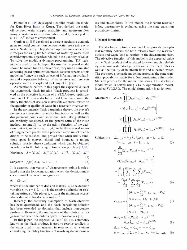
flowchart, VLGA is used for reducing the convergence timeof the model. As the SVLGAQ model does not directly usethe inflow time series, the chromosome length is sequen-tially increased by increasing in the number of seasons.For example, in the first step, the reservoir operating andwaste load allocation rules are developed for two seasons

per year. Therefore, each chromosome includes ni · nj ·(P + G) · 2 genes. Then the number of seasons is increasedand the previous optimal seasonal rules are considered asthe initial solution for next computational step. Thissequential procedure finally provides the monthly operat-ing rules for reservoir outlets and treatment plants. In the

Fig

.2.

Gen

eva

lues

inth

ech

rom

oso

mes

of

SV

LG

AQ

mo

del

.


last step, the number of genes in each chromosome is equalto ni · nj · (P + G) · m.

In this study, different components of the VLGA havebeen developed with the following characteristics:

5.1. Encoding of decision variables

In GAs, an encoded decision variable is referred to asgene and a string of genes (chromosome) represents onepossible solution to the problem. Fig. 2 shows the Genes’value in the proposed stochastic VLGA-based optimizationmodel.

In this paper, a binary coding is used to represent thevalue of genes. In the binary encoding method, the largejumps in variable values between generations can be limitedusing gray coding proposed by Goldberg [19]. In gray cod-ing, used in this study, the binary representation of eachvariable changes in each sequence with no more than onebinary digit. This binary encoding and discretization ofdecision variables can effectively reduce the computationalrun time of the problem.

5.2. Selection

In the so called ‘‘Mimicking the biological process’’ ofthe survival of the fittest individuals, the solutions thathave a higher level of fitness, are more likely to be selected.In this study, the fitness of each chromosome in the popu-lation is calculated using the reservoir–river water qualitysimulation model. The simulation model calculates thetemporal variation of the concentration of water qualityvariables in different layers of reservoir, release from differ-ent outlets, and along downstream river system. The fitnessof each chromosome is also calculated based on theexpected value of the Nash product (Eq. (4)).

Cantu’-Paz [6] presented the main characteristics ofsome useful chromosome selection methods such as Rou-lette Wheel, Tournament, Linear Ranking, ExponentialRanking, and Truncation Selection. In this paper, theTournament selection, which has been widely used in liter-ature such as Burn and Yulianti [4], is used in the GA-based optimization model.

5.3. Cross-over and mutation

Cross-over and mutation operators are used for creatingnew chromosomes. There are several cross-over methodssuch as one-point, two-point, and uniform cross-over,but there is no consensus among investigators, whetherthere is a generally superior cross-over method. Cross-overoccurs, with a pre-specified probability (Pc), between twoselected chromosomes. One point cross-over, which is usedin this study, randomly chooses a position (gene) in thechromosome and new chromosomes are obtained by swap-ping all genes after that position.

Mutation is an important process that prevents prema-ture convergence to local optimal solutions. The mutation


operator changes the bit from ‘‘1’’ to ‘‘0’’ or visa versa withprobability Pm.

6. Case study

The proposed optimization/simulation procedure isused for water quality management in the Ghomrud Reser-voir–River system in the central part of Iran. The 15-Khor-dad Dam which has been built on Ghomrud River is anearth-fill dam with a volume of 200 million cubic meters.This reservoir–river system supplies the water for domestic,industrial and agricultural sectors. The main characteristicsof the 15-Khordad Dam are presented in Table 1. Themean annual flow of the river is 177 million m3. The mainwater user is the city of Ghom with 8000 ha of agriculturallands. Total downstream water demand is about 100 mil-lion m3 per year.

The main problem of 15-Khordad reservoir is highTotal Dissolved Solids (TDS) concentration which is dueto saline inflow, salinity of geological formations in the res-ervoir bed as well as the upstream basin. The Dam wasconstructed in 1994 and the reservoir water degradationwas observed only 2 years after operation so that the qual-ity of allocated water to domestic and agricultural demandsis violating the standards.

Water quality data is scarce in this region and the waterquality of the reservoir was monitored by the nationalWater Research Center in the water year 1997–1998. Watertemperature, Electrical Conductivity (EC), and DissolvedOxygen (DO) have been monitored in 13 cross-sectionsselected along the reservoir stretch. In each cross-section,data was gathered from surface water and points locatedin a vertical plane in reservoir depth with 2 m increments.The analysis of monitoring data shows that the horizontalvariations of the water quality constituents are negligible,and a one-dimensional water quality simulation modelcan be used for reservoir water quality simulation. Theconcentration of DO has always satisfied the standardsdue to limited nutrient loads. Therefore, in this study watertemperature and TDS are considered as the water qualityindicators.

Ghomrud River in downstream of reservoir is polluteddue to discharge of the return flows of two main agricul-tural/industrial regions namely Salafchegan and Ghom

Table 1The main characteristics of the 15-Khordad Dam [26]

Parameter Value

Total volume 200 million m3

Reservoir length at normal water level 12 kmDead volume 35 million m3

Foundation elevation 1357.5a

Crest elevation 1448.6 ma

Normal water level 1440.5 ma

Spillway elevation 1440.5 mSpillway capacity 1417.6 m3/s

a From sea level.

located at 32 and 72 km downstream of the reservoir,respectively (see Fig. 3). The SVLGAQ model is used todetermine the selective withdrawal and waste load alloca-tion policies for water quality management in the reser-voir–river system. However some structural pollutioncontrol methods such as diverting upstream saline tributar-ies can be used for water quality management in thissystem.

As can be seen in Table 1, the reservoir has two out-lets and one freefall spillway, which can be used for selec-tive withdrawal and controlling the downstream waterquality.

After consultation with the experts in different sectorsas well as considering the physical characteristics of thesystem, the utility functions of different decision makersand stakeholders of the system are formulated as follows[26]:

f1;mðRm;yÞ¼Rm;y=Dm if Rm;y6Dm

1 otherwise

�8m;y ð36Þ

f2;mðSmþ1Þ¼ðSmþ1�35Þ=ð95Þ if 356Smþ16130

1 otherwise

�ð37Þ

f3;mð�cm;hÞ¼

0 if �cm;h>3000

1� �cm;h�1200

3000�1200if 12006�cm;h63000

1 if 11006�cm;h<1200

0:9þ 0:1��cm;h

1100

� �if �cm;h<1100

8h;m¼3; . . . ;11

8>>>>>>><>>>>>>>:ð38Þ

f3;mð�cm;hÞ¼�cm;h=1900 if �cm;h<1900 m¼12;1;2

1 if �cm;h P1900 8h

�ð39Þ

f4;mð�em;gÞ¼1 if �em;g610�1�ð�em;g�10Þð100�10Þ þ1 if �em;g >10

(8g;m ð40Þ

where Dm is the water demand in month m (million cubicmeters). Eq. (36) is set by the Water Supply Agency andshows the utility of this agency and the water users as afunction of the allocated water in each month. The Reser-voir Operator sets a utility function as expressed in Eq. (37)that is related to the available monthly water storage. Con-sidering the high capacity of the spillway and the annualwater demand, the value of utility function of this deci-

Parameter Value

Flood control bottom outlet elevation 1408 ma

Flood control bottom outlet capacity 94 m3/sUpper outlet elevation 1415 ma

Lower outlet elevation 1430 ma

Upper outlet capacity 8 m3/sLower outlet capacity 8 m3/sWater surface area at normal water level 14 km2

Minimum operational water level 1420 ma

ShoorRiver

GhomrudRiver

DarbandRiver

GolpayeganDam

15-KhordadDam

ReyhanRiver

Ghom City and GhomAgricultural/Industrial

Region

SalafcheganAgricultural/Industrial

RegionN

Fig. 3. Ghomrud Reservoir–River system in central Iran.


sion-maker is 1 for water storages more than 130 millioncubic meters and is less than 1 for water storages between35 (dead storage) and 130 million cubic meters. Eqs. (38)and (39) are set by the Health Department and the Envi-ronmental Protection Agency. Eq. (38) forces the modelto provide water releases with lower salinity during themonths of March to November, when the water releasequantity is important. Based on Eq. (39), the reservoir re-lease in the months of December–February, when there isa little water demand, can be used for scouring the reser-voir and controlling the salinity build-up. In these3 months, water demands can be supplied using groundwa-ter resources. Eq. (40) presents the utility function of thepollution dischargers for controlling pollution sourceswhich are mainly the return flow from irrigation networks.High potential of evaporation (more than 3200 mm/year)and considerable costs of TDS removal justify the diver-sion of a fraction of discharging wastewater/return flow

to the evaporation ponds. This polluters’ utility functionis usually set based on the construction and operationalcosts of the evaporation ponds.

7. Results and discussion

Analysis of water quality monitoring data shows thatthe reservoir experiences only one turnover per year whichis usually in February. The strongest thermal stratificationis observed in August, when the maximum differencebetween the water temperatures in different layers is usuallymore than 15 �C. This thermal stratification results in a dif-ferent effective diffusion coefficient as well as a differentTDS concentration in the reservoir depth. Water qualitymonitoring data shows that the thermocline depth can varyfrom 13 to 20 m when there is a thermal stratification in thereservoir. The maximum vertical density gradient occurs atthe thermocline depth. The saline inflow is usually allo-


cated to the upper layers during the summer monthsdue to the similarity between their water temperaturesand densities. Therefore, the TDS concentration in the epi-

June 17,

January

0

5

10

15

20

25

30

0 10 15 20 25 30

Temp. (C)

Dep

th (

m)

0

5

10

15

20

25

30

0 10 15 20 25 30

Dep

th (

m)

Simulated

Observed

Temp. (C)

Simulated

Observed

5

5

Fig. 4. Some comparisons between the observed and simulated va

limnion (a reservoir volume located above thermocline) ismore than hypolimnion (a reservoir volume located belowthe thermocline depth) during the summer months.

0

5

10

15

20

25

30

0 500 1000 1500 2000 2500

TDS (mg/L)

Dep

th (

m)

Simulated

Observed

1997

19, 1998

0

5

10

15

20

25

30

0 500 1000 1500 2000 2500

Dep

th (

m)

Simulation

Observed

TDS (mg/L)

lues of the water quality variables in the verification process.

500

1000

1500

2000

2500

Jan-68

Jan-69

Jan-70

Jan-71

Jan-72

Jan-73

Jan-74

Jan-75

Jan-76

Jan-77

Jan-78

Jan-79

Jan-80

Jan-81

Jan-82

Jan-83

Jan-84

Jan-85

Jan-86

Jan-87

Jan-88

Jan-89

Jan-90

Jan-91

Jan-92

Jan-93

Jan-94

Jan-95

Jan-96

Jan-97

Month

TD

S (

mg

/L)

SVLGAQ SVLGA

Fig. 5. Comparison between the reservoir release salinity in the SVLGAQ and SVLGA models in months of March–November during the planninghorizon (360 months).

600

1100

1600

2100

2600

Jan-68

Jan-69

Jan-70

Jan-71

Jan-72

Jan-73

Jan-74

Jan-75

Jan-76

Jan-77

Jan-78

Jan-79

Jan-80

Jan-81

Jan-82

Jan-83

Jan-84

Jan-85

Jan-86

Jan-87

Jan-88

Jan-89

Jan-90

Jan-91

Jan-92

Jan-93

Jan-94

Jan-95

Jan-96

Jan-97

Month

TD

S (

mg

/L)

SVLGAQ SVLGA

Fig. 6. Comparison between the release salinity in the SVLGAQ and SVLGA models only in the months of March–November in the planning horizonwhen the release salinity in the SVLGA model is more than the standard level (1100 mg/l).


nth

em

on

thly

aver

aged

rele

ase

sali

nit

yin

SV

LG

Aan

dS

VL

GA

Qm

od

els

(mg/

l)[2

6]

ryF

ebru

ary

Mar

chA

pri

lM

ayJu

ne

July

Au

gust

Sep

tem

ber

Oct

ob

erN

ove

mb

erD

ecem

ber

Ave

rage

inth

em

on

ths

of

Mar

ch–N

ove

mb

er

Ave

rage

inth

em

on

ths

of

Dec

emb

er–F

ebru

ary

1416

.613

06.3

1249

.312

36.5

1294

.513

48.5

1340

.513

61.6

1456

.114

56.6

1506

.813

3914

6614

91.9

1318

.012

59.6

1241

.712

51.2

1253

.912

90.5

1317

.613

52.4

1392

.415

76.4

1297

.515

37.5


The proposed simulation model is calibrated using thedata of the first 3 months of the monitoring period (April1997 to June 1997) and its performance is verified usingthe rest of the existing water quality data (July 1997 toMarch 1998). Fig. 4 shows a sample of comparisonsbetween the observed and simulated values of water qualityvariables in the verification process. The calibrated valuesof the simulation model parameters are presented inTable 2. The results show that the simulation models canbe effectively used for water quality management in thisreservoir–river system.

In this case study, 30 years of monthly water quality andquantity data (1968–1997) is used for reservoir operationand waste load allocation in the river downstream of thereservoir. The state transition probability matrix for inflowis also set using this monthly inflow time series. The num-ber of characteristic values for reservoir storage and infloware considered to be equal to 32 and 9, respectively.

After consultation with the decision makers in differentsectors and considering their relative authorities, the initialvalues for wr, ws, wc and we are assumed to be equal to 0.15,0.05, 0.56, and 0.24, respectively [26].

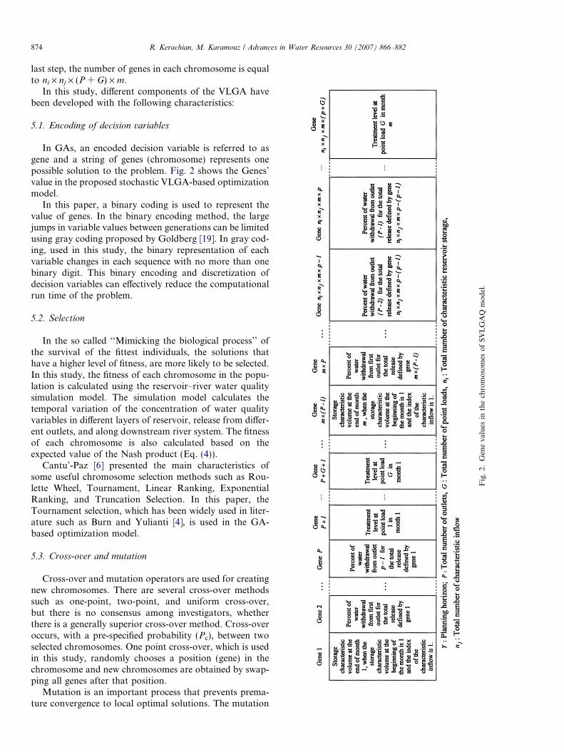
Both SVLGAQ and SVLGA models can completelysupply the downstream water demands. Also as it is shownin Figs. 5 and 6, the SVLGAQ model can considerablyimprove the release salinity. Considering the utility func-tions, in the months of December, January, and February,the SVLGAQ model usually provides more saline releasedue to the scouring and flushing of the reservoir. But inother months, it results in improvements in release salinity.As can be seen in Fig. 6 and Table 3, in months of Marchto November, when the downstream water quality is veryimportant, the average release salinity of the SVLGAQmodel is less than the release salinity of the SVLGA model.As limit of the release salinity is set as 1100 mg/l, Fig. 6presents only the values which are more than this standardlevel (1100 mg/l). As it is shown in this figure, the averageand maximum reduction in monthly release salinity are100 mg/l and 600 mg/l, respectively.

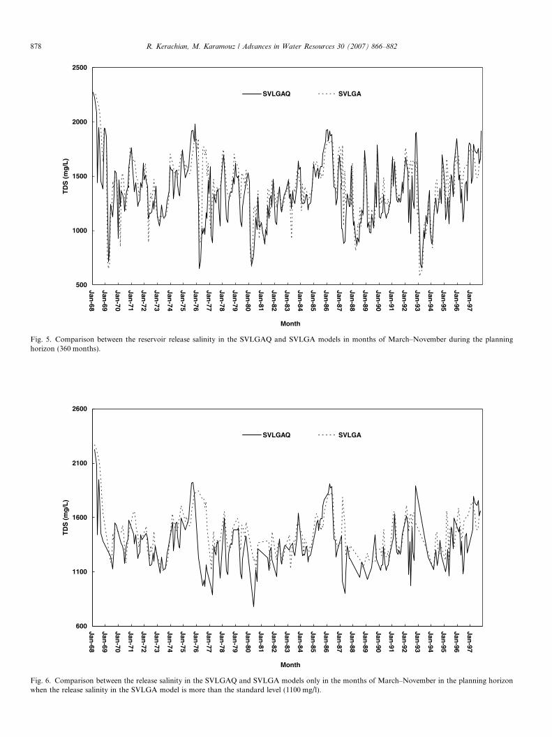
Fig. 7 shows the importance of simultaneous selectivewithdrawal and waste load allocation in improving thedownstream water quality. In this figure, two time seriesof the TDS concentration at a local monitoring station(immediately downstream of Ghom point load) are pre-sented which have been obtained by simulating the operat-ing rules of the Reservoir model (SVLGAQ-R) andReservoir–River model (SVLGAQ-RR). SVLGAQ-RRmodel considers all utility functions which are related tothe reservoir operation and waste load allocation while inSVLGAQ-R model waste load allocation is not considered(third bracket in Eq. (4) is omitted) and it only presents the

Tab

le3

Co

mp

aris

on

bet

wee

Mo

nth

Jan

ua

SV

LG

A14

74.5

SV

LG

AQ

1544

.4

Table 2The calibrated values of the simulation model parameters [26]

A1 (m2/s) A3 (m2/s) Ec (1/m) b (%) Secchi depth (m)

0.5 · 10�5 �0.7 2 · 10�6 0.55 2.5

0

500

1000

1500

2000

2500

3000

3500

4000

Ma

r-68

Ma

r-69

Ma

r-70

Ma

r-71

Ma

r-72

Ma

r-73

Ma

r-74

Ma

r-75

Ma

r-76

Ma

r-77

Ma

r-78

Ma

r-79

Ma

r-80

Ma

r-81

Ma

r-82

Ma

r-83

Ma

r-84

Ma

r-85

Ma

r-86

Ma

r-87

Ma

r-88

Ma

r-89

Mar-90

Ma

r-91

Ma

r-92

Ma

r-93

Ma

r-94

Mar-95

Mar-96

Mar-97

Month

TD

S (

mg

/L)

SVLGAQ-RRSVLGAQ-R

Fig. 7. Time series of TDS concentration at the Ghom Monitoring Station based on SVLGAQ-R and SVLGAQ-RR operating rules (excluding the valuesrelated to the months of December–February).


reservoir operating rules considering the water qualityissues. The TDS concentration in the river can be decreasedup to 1000 mg/l during summer months as a result of uti-lizing reservoir operation and waste load allocation poli-cies, while water demands are completely supplied.

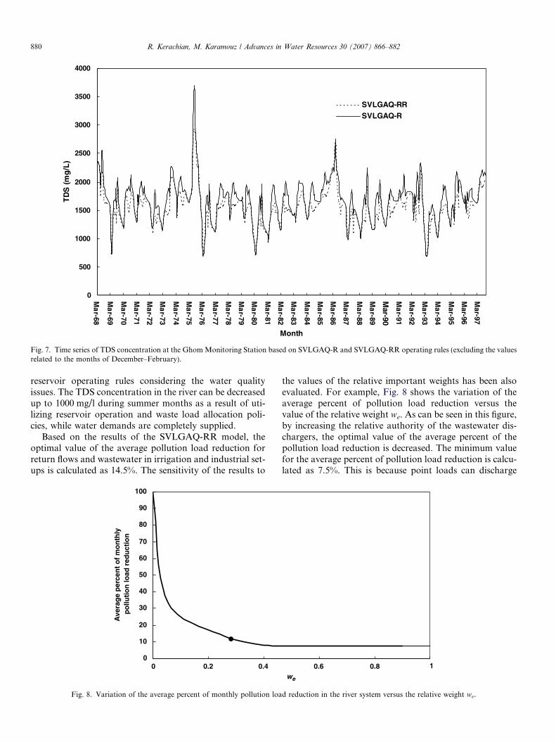
Based on the results of the SVLGAQ-RR model, theoptimal value of the average pollution load reduction forreturn flows and wastewater in irrigation and industrial set-ups is calculated as 14.5%. The sensitivity of the results to

0

10

20

30

40

50

60

70

80

90

100

0 0.2 0.4

Ave

rag

e p

erce

nt

of

mo

nth

lyp

ollu

tio

n lo

ad r

edu

ctio

n

•

Fig. 8. Variation of the average percent of monthly pollution loa

the values of the relative important weights has been alsoevaluated. For example, Fig. 8 shows the variation of theaverage percent of pollution load reduction versus thevalue of the relative weight we. As can be seen in this figure,by increasing the relative authority of the wastewater dis-chargers, the optimal value of the average percent of thepollution load reduction is decreased. The minimum valuefor the average percent of pollution load reduction is calcu-lated as 7.5%. This is because point loads can discharge

0.6 0.8we

1

d reduction in the river system versus the relative weight we.

Table 4Average percent of pollution load reduction in point sources located in the study area corresponding to sample point A on trade-off curve (Fig. 8)

Month January February March April May June July August September October November December

Percent of pollutionload reduction

0 0 10 10 13 27 32 34 26 13 10 0

800

1000

1200

1400

1600

1800

2000

2200

2400

0 0.1 0.2 0.3 0.4 0.5 0.6 0.7 0.8 0.9 1

we

Max

imu

m m

on

thly

vio

lati

on

(m

g/L

)

0

20

40

60

80

100

Nu

mb

er o

f vi

ola

tio

ns

du

rin

gp

lan

nin

g h

ori

zon

(m

on

th)

Maximum violation

Number of violations

Fig. 9. Variation of the number of violations (month) and the maximum value of monthly violations (mg/l) versus the relative weight we (excludingviolations occurred in the months of December–February).


wastewater with no control/treatment in the months ofDecember–February (see Eq. (39)), and the minimum valueof em,y in the other months is equal to 10% (see Eq. (40)).

Table 4 presents the monthly average percent of pollu-tion load reduction at point loads corresponding to thesample point A on the trade-off cure (Fig. 8). As presentedin this table, the optimal average percents of pollution loadreduction in the months of December–February are equalto zero. These months are used for controlling the salinitybuild up in the reservoir and the released water is not allo-cated to demands. Therefore, based on Eq. (40), pollutionloads can be discharged with minimum level of control.

In general, frequency, duration, and magnitude ofviolation of water quality standards are the performanceindicators which present the reliability, resiliency and vul-nerability of water quality management policies. The reli-ability indicator describes how likely or often the waterquality goals may be achieved, while resiliency and vulner-ability indicators represent how quickly the water qualitysystems recovers from a failure and the severity of theconsequences of violations of water quality standards,respectively. The performance of the proposed selectivewithdrawal and waste load allocation policies have beenevaluated using these criteria. As an example, Fig. 9 pre-sents the variation of the number of violations (an indexof reliability) and the maximum value of monthly violation(an index of vulnerability) versus we.

To evaluate the effectiveness of the SVLGAQ model inreducing the computational time, it has been comparedwith the classic Genetic Algorithm optimization model.

The proposed model can reduce the computational timeby a factor of 3.

8. Summary and conclusion

The methodology of combining a water quality simula-tion model with a stochastic GA-based optimization modelhas been demonstrated to generate the improved opera-tional strategies for water quality management in reser-voir-river systems. In this paper, the Nash bargainingtheory was used to resolve the existing conflict of interestsas different decision-makers and stakeholders are involvedin the water quantity/quality management in the system.The utility functions of the proposed models were devel-oped based on the reliability of supplying water demands,water storage, in-stream flow and allocated water qualityas well as the rate of wastewater pollution control.

The expected value of the Nash product was consideredas the objective function of the model which can incorpo-rate the inherent uncertainty of the reservoir inflow. Toreduce the computational burden of the GAs, the conceptof Sequential Game theory was used to develop a new ver-sion of Genetic Algorithms for this stochastic reservoir–river operation problem.

The proposed model was applied to a reservoir–riversystem in the central part of Iran. The results showed thatthe model can reduce the salinity of the allocated water todifferent water demands as well as the salinity build-up inthe reservoir. Based on the proposed reservoir operationand waste load allocation rules, the average and maximum


salinity reduction in the river are equal to 210 and1000 mg/l, respectively.

The results also showed the significant value of using amodified Genetic Algorithm in the reduction of the compu-tational run time of the alternative quantitative–qualitativereservoir operation and waste load allocation models.

Acknowledgments

Parts of this paper were presented at the ASCE WorldWater and Environmental Resources Congress 2004 [22]and the Sixth International Conference on Hydro-infor-matics [23].

References

[1] Boner MC, Furland LP. Seasonal treatment and variable effluentquality based on assimilative capacity. Res J Water Pollut ControlFed 1982;54:1408–16.

[2] Brown LC, Barnwell O. The enhanced stream water quality models,QULA2E and QUAL2E-UNCAS: documentation and user manual.EPA, 1987.

[3] Burn DH. Water quality management through combined simulation–optimization. J Environ Eng, ASCE 1989;115(5):1011–24.

[4] Burn DH, Yulianti S. Waste-load allocation using genetic algorithms.J Water Res Plan Manage, ASCE 2001;127(2):121–9.

[5] Sharon G, Campbell SG, Hanna RB, Flug M, Scott JF. ModelingKlamath River system operation for quantity and quality. J WaterRes Plan Manage, ASCE 2001;127(5):284–94.

[6] Cantu’-Paz E. Order statistics and selection methods of evolutionaryalgorithms. Info Proc Lett 2002;82:15–22.

[7] Chaves P, Tsukatani T, Kojiri T. Operation of storage reservoir forwater quality by using optimization and artificial intelligencetechniques. Math Comput Simulat 2004;67:419–32.

[8] Dandy G, Crawley P. Optimum operation of a multiple reservoirsystem including salinity effects. Water Resour Res 1992;28(4):979–90.

[9] De Azvedo LGT, Gates TK, Fontane DG, Labadie JW, Porto RL.Integration of water quantity and quality in strategic river basinplanning. J Water Res Plan Manage 2000;126(2):85–97.

[10] Denicolo V, Mariotti M. Nash bargaining theory, nonconvexproblems and social welfare orderings. Theory Decision 2000;48:351–8.

[11] Ellis JH. Stochastic water quality optimization using imbeddedchance constraint. Water Resour Res 1987;23(12):2227–338.

[12] Fahmy HS, King JP, Wentzel MW, Seton JA. Economic optimizationof river management using genetic algorithms. Paper No. 943034,ASAE 1994 int summer meeting, St. Joseph, Mich, 1994.

[13] Ferrara RA, Dimino MA. A case study analysis for seasonalnitrification: economic efficiency and water quality preservation.Res J Water Pollut Control Fed 1985;57:763–9.

[14] Fontane D, Labadie JW, Loftis B. Optimal control of reservoirdischarge quality through selective withdrawal. Water Resour Res1981;17(6):1594–604.

[15] Fujiwara O, Puangmaha W, Hanaki K. River basin water qualitymanagement in stochastic environment. J Environ Eng, ASCE1988;114(4).

[16] Ganji A, Khalili D, Karamouz M. Development of stochasticdynamic Nash game model for reservoir operation. I: The symmetricstochastic model with perfect information. Adv Water Resour, inpress, doi:10.1016/j.advwatres.2006.04.004.

[17] Ganji A, Karamouz M, Khalili D. Development of stochasticdynamic Nash game model for reservoir operation. II: The value of

players’ information availability and cooperative behaviors. AdvWater Resour, in press, doi:10.1016/j.advwatres.2006.03.008.

[18] Gen M, Cheng R. Genetic algorithm and engineering optimiza-tion. Wiley Europe Publication; 2000. p. 512.

[19] Goldberg DE. Genetic algorithms in search, optimization andmachine learning. Reading, MA: Addison-Wesley; 1989. p. 399.

[20] Harsanyi JC, Selten R. A generalized Nash solution for two-personbargaining games with incomplete information. Manage Sci1972;18:80–106.

[21] Hydrologic Engineering Center (HEC), HEC-5Q simulation on floodcontrol and conservation systems, appendix on water quality analysis,1992.

[22] Karamouz M, Kerachian R. Optimal operation of reservoir systemsconsidering the water quality: application of stochastic sequentialgenetic algorithms. In: Proceedings of ASCE World water andenvironmental resources congress 2004, Salt Lake City, Utah, 2004.

[23] Karamouz M, Kerachian R. Optimal reservoir operation consideringthe water quality. In: Proceedings of hydro-informatics 2004, Singa-pore, 2004.

[24] Karamouz M, Vasiliadis H. A Bayesian stochastic optimization ofreservoir operation using uncertain forecast. Water Resour Res1992;28(5).

[25] Kerachian R, Karamouz M. Waste-load allocation model forseasonal river water quality management. Scientia Iranica2005;12(2):117–30.

[26] Kerachian R. Water quality management in river–reservoir systems.PhD dissertation, Department of Civil and Environmental Engineer-ing, Amirkabir University (Tehran Polytechnic), Teheran, Iran, 2004.

[27] Labadie JW. Optimal operation of multi-reservoir systems: state-of-the-art review. J Water Resour Plan Manage, ASCE2004;130(2):93–111.

[28] Lence BJ, Takyi AK. Data requirements for seasonal dischargeprograms: an application of a regionalized sensitivity analysis. WaterResour Res 1992;28(7):1781–9.

[29] Loftis B, Labadie JW, Fontane D. Optimal operation of a system oflakes for quality and quantity. In: Proceedings of specially conferenceon computer applications in water resources, Buffalo, NY, 1985.

[30] Michalewicz Z. Genetic algorithms + data structure = evolutionprograms. New York: Springer; 1992.

[31] Mousavi SJ, Karamouz M, Menhaj MB. Fuzzy-state stochasticdynamic programming for reservoir operation. J Water Resour PlanManage, ASCE 2004;130(6):460–70.

[32] Nandalal KDW, Bogardi JJ. Reservoir management for improvingriver water quality. In: Proceedings of water resources managementunder drought or water storage conditions, Rotterdam, 1995. p. 257–64.

[33] Nash JF. The bargaining problem. Econometrica 1950;18:155–62.[34] Oliveira R, Loucks DP. Operating rules for multi-reservoir systems.

Water Resour Res 1997;33(4):839–51.[35] Palmer RN, Ryu J, Jeong S, Kim YO. An application of water

conflict resolution in the Kum river basin, Korea. In: Proceedings ofASCE environmental and water resour inst conf, Virginia, May 2002,p. 19–22.

[36] Richards A, Singh N. Two level negotiations in bargaining overwater. In: Proceedings of the international game theory conference,Bangalore, India, 1996. p. 1–23.

[37] Shahidehpour M, Yamin H, Li Z. Market operations in electricpower systems. New York: John Wiley and Sons; 2001. p. 191–232.

[38] Takyi AK, Lence BJ. Markov chain model for seasonal water qualitymanagement. J Water Resour Plan Manage, ASCE1995;121(2):144–57.

[39] Wardlaw R, Sharif M. Evaluation of genetic algorithms for optimalreservoir system operation. J Water Resour Plan Manage Div AmSoc Civ Eng 1999;125(1):25–33.

[40] Willey RG, Smith DJ, Duke Jr H. Modeling water resources systemsfor water-quality management. J Water Resour Plan Manage, ASCE1996;122(3):171–9.

http://dx.doi.org/10.1016/j.advwatres.2006.04.004

http://dx.doi.org/10.1016/j.advwatres.2006.03.008

A stochastic conflict resolution model for water quality management in reservoir–river systems

Documents

Transcript of A stochastic conflict resolution model for water quality management in reservoir–river systems