Probab. Th. Rel. Fields 81, 1-10 (1989) Probability Theory a.d Related Fields

�9 Springer-Verlag 1989

A Stationary, Pairwise Independent, Absolutely Regular Sequence for which the Central Limit Theorem Fails*

Richard C. Bradley Department of Mathematics, Indiana University, Bloomington, Indiana 47405, USA

Summary. A strictly stationary finite-state non-degenerate random sequence is constructed which satisfies pairwise independence and absolute regularity but fails to satisfy a central limit theorem. The mixing rate for absolute regularity is only slightly slower than that in a corresponding central limit theorem of Ibragimov.

1. Introduction

Suppose (Xk, kE~ r) is a strictly stationary sequence of pairwise independent random variables. By Etemadi [5, Theorem lJ, if E IXot < oo then (Xk) satisfies the strong law of large numbers. However, if EXg < oe and Var X o > 0, it does not follow that (Xk) satisfies the central limit theorem. Indeed, Janson [-8, Exam- ple 3] has constructed counterexamples with X o having an arbitrary distribution with finite second moment. The purpose of this note is to construct a counterex- ample which (in addition to pairwise independence) has some strong mixing properties. Our main result is Theorem 1 below.

The author owes a big debt to Professor Robert Burton. Two years ago Burton showed the author a (pairwise independent, non-ergodic) apparent 2- state counterexample (for which the failure to satisfy the CLT intuitively seemed likely but was not rigorously verified). This helped to lead the author to a two-state ergodic counterexample (constructed in Sect. 2 below). (According to a trusted source, such examples were apparently already known but not well publicized.) This in turn led to the main result of this note.

First let us define the mixing condition. Suppose X :=(XR, k~Z) is a strictly stationary sequence of random variables on a probability space (f2, Y, P). For - oo _< J_< L_< ~ let ~jL denote the o--field generated by (Xk, J-< k_< L). For n = 1, 2, 3, ... define

I J

fi(n)=fi(X, n).'=sup�89 ~ ~ IP(Aic~B~)--P(Ai)P(Bj)I (1.1) i= l j = l

* This work was partially supported by NSF grant DMS 86-00399

2 R.C. Bradley

where this sup is taken over all pairs of finite partitions {A1 . . . . , AI) and {B1, ..., Bs} of O such that Aie~-~ for all i and B j ~ ~ for all j. The sequence X is said to satisfy "absolute regularity" [-10, 11] if f l (n)~ 0 as n ~ 0o.

For partial sums we use the notation S,.'=X1 + . . . + X,. Also, the notation " ~ " means 0 (').

Theorem 1. There exists a strictly stationary sequence X:=(Xk, k~TZ) such that the following statements hold:

X o takes only three values ( - 1 , O, and 1, with

P(Xo=O)=I /2 and P ( X o = - I ) = P ( X o = I ) = I / 4 ) ; (1.2)

V n~=O, X o and X n are independent; (1.3)

fl(n) ~ 1/n as n ~ 0o; (1.4)

[- inf P (Sn = 0)] > 0; and (1.5) n__>l

the family of r.v. 's (S~, n = 1, 2 . . . . ) is tight. (1.6)

By (1.5), S, cannot become asymptotically normal under any kind of normal- ization.

Let us briefly consider the class of known stationary absolutely regular sequences (Xk) which fail to satisfy the CLT. In the examples of Herrndorf [6] and Bradley [2, Theorems 1, 2, 7] the Xk'S are uncorrelated (but not pairwise independent). In the case where the Xk'S are bounded (with or without being uncorrelated), the mixing rate in (1.4) is the fastest that has been obtained so far - but only slightly faster than the rates obtained earlier in Davydov [4, Example 2] and Bradley [2, Theorem 2]. As a special case of a result of Ibragi-

mov in [7, Theorem 18.5.4], the mixing rate ~ fl(n)< oe together with (1.2)-(1.3) n = l

would imply the CLT. There still remains a slight gap between Ibragimov's rate and (1.4). (It should perhaps be mentioned that Davydov [-4] and Herrndorf [6] discussed the "strong mixing" condition instead of absolute regularity, but their arguments extend directly to absolute regularity. Also, a mistake in Bradley [2] - the attributing to M.I. Gordin of a misstatement of one of his results - is corrected in [3].)

The main idea of our construction - the use of a function of a "renewal type" Markov chain - comes from Davydov [4]. We shall adapt Davydov's [-4] method of estimating dependence coefficients. We shall adapt an idea of H.C.P. Berbee (from his own construction given in [-1, Theorem 11]) which con- verted [4, Example 2] from a bounded countable-state example to a finite-state one. Also we shall adapt an idea of Herrndorf [6] which achieved (1.5) and (1.6) in his own counterexample.

The proof of Theorem 1 will be given in Sect. 3, based on preliminary work done in Sect. 2.

Sequence for which the CLT Fails 3

2 . P r e l i m i n a r i e s

In this section some random sequences will be constructed and some lemmas will be given. This material will be used in Sect. 3 in the proof of Theorem 1.

D e f i n i t i o n 2.1. (a) Let ~ denote the set of all ordered pairs (t, u) such that

ts{2, 4, 8, 16, 32, ...} vo {--2, --4, --8, -- 16, --32, ...} and

us{0, 1, 2, ..., I t l - 1 }.

(b) Let # denote the probability measure on 5 ~ defined by

#({(t, u)})= 1/(2t 2) g (t, u)s 5/'.

In what follows, for s s 5 '~, the quantity #({s}) will be written simply as #(s). (c) Let (Vk, ks~g), with Vk:=(Tk, Uk) g ks2g, be a strictly stationary Markov

chain with state space 5 t', with invariant marginal probability measure #, and with one-step transition probabilities given by the following equations:

P(Vl=(t, ltl-1)]Vo=(T,O))=3/(2t 2) gt , T= __.2, ___4,_+8, -t-16 . . . . ;

P(Vl=(t,u--1)lVo=(t,u))=l Vt=_+2, +4, ___8 . . . . V u = l , 2, 3 . . . . . [ t [ -1 ;

P(V1 =s l [ Vo =So)=0 for all other pairs of states so, s165 ~

(d) Define the function f :

1 if

- - 1 if f((t, u)):=

- - 1 if

1 if

5P--, { - 1 , 1} as follows:

t = 2 , 4 , 8 . . . . and t/2<=u<t;

t = 2 , 4 , 8 . . . . and O<_<u<t/2;

t = - 2 , - 4 , - 8 . . . . and [t]/2<=u<[t[;

t = - 2 , - 4 , - 8 . . . . and O<u<[t[/2.

(e) Define the (strictly stationary) sequence (Wk, ks7Z) as follows:

V ksZ , Wk = f (Vk).

Remark 2.2. Referring to Definition 2.1(c) we shall henceforth assume that for every cosf2, every ks2g, the ordered pair (Vk, Vk+ 1)(CO) is either ((T, 0), (t, [ t l - 1)) for some numbers T, t = +_2, _+4, +8, ... or else ((t, u), (t, u - 1 ) ) for some t = ___2, __4, ___8 . . . . . u = l , 2 . . . . , Jt[--1. For a given cosY2, if I < J are integers such that

Ui(oo)=Us(co)=O and Uk(CO)=#O V k = I + l , . . . , J - - 1 ,

then J - I s { 2 , 4, 8, ...},

(V,+ 1, I/i+ 2 . . . . . Vs)(oo)=((t, t - - l ) , (t, t--2) . . . . . (t, 0)) or

((-t , t-1), ( - t , t - 2), ..., ( - t , O)) for t = a - I ,

4 R.C. Bradley

and (W~+I, Wt+2 . . . . . Wa)(co)=(1 . . . . . 1, - 1 , ..., - 1 ) (with (J-1)/2 l 's and (J -1)/2 - l 's in either case).

Note that by Definition 2.1(b)(c),

or ( - 1 , ..., - 1 , 1 . . . . ,1)

P(Uo=O)=t~({(t,O): t = _+2,-t-4, +8 . . . . })=1/3. (2.1)

In what follows, the notation a(...) means the a-field generated by (...). The following lemma will be helpful.

Lemma 2.3. Suppose A~a(Vk, k<O), B~a(Vk, k > l), and P(A~{Uo=O})>O. Then P(BIA m (Uo =0})=P(BI Uo =0).

The proof is elementary. One first verifies the lemma for the special case where A={To=t} and B={VI=s} where t=_+2, _+4, _+8 . . . . and s~SP; and then one uses the Markov property.

For any integers I < J define the event

D(I, J)..={Ut = Us=O, Uk=4=O V k, I <k <J}. (2.2)

(By Definition 2.1 and Remark 2.2, this event is non-empty only if J - I =2, 4, 8, 16 . . . . ). It is easy to see that if L is a positive integer and 0 < n < 2 L, then

P(W, = 1 I D(0, 2L)) = P(W, = -- 1 I D(0, 2L)) = 1/2.

Hence by stationarity we have

L e m m a 2.4 . P(Wo = 1 ) = P ( W o = - 1 ) = 1 /2 .

Lemma 2.5. Suppose n > 1. Then

P(Wo =4:: W~ I Uk=O for some k=0 , 1, ..., n - 1)= 1/2, and

P(Wo, w.I vk4=0 vk=0 , 1, ..., n - 1)= 1/2.

Proof. The first equation is elementary. We shall just prove the second. Define the event D:={Ukq=O Vk=0, 1, . . . , n - - l} . Let L be the positive integer such that 2 L- 1 < n < 2 z. The event D can be partitioned into events D (I, I + 2') where I < 0 and I+2'>n (which forces l>L). For such an I and l,

D(I, I + 2 ' ) = {U,=0, IT~+11=2 ̀} and hence

P(D(I, I +2')) = P(UI =0) . P(I T,+ 11 = 2'1 U~ =0)

= (1/3). (3/4') = 1/4' (2.3)

by Definition 2.1(c) and (2.1). Hence

- 1

P(D)= ~ ~" P(D(I, 1+2')) ' = L I = n - - 2 z

= 2. [-2- L _ (2 n/3). 4- L]. (2.4)

Sequence for which the CLT Fails 5

Next , the event {W o + W~} m D can be par t i t ioned into events D(I, 1 + 2 ' ) where l > L, I < 0, I + 2 t > n and 0 < I + 2 ' - 1 < n. (This last equat ion follows f rom Remark 2.2.) Fo r l=L, the condi t ions on I are (equivalent to) n - 2 r < I < 0 . F o r l > L + 1, the condi t ions on I are (equivalent to) - 2 t- 1 =< I < n - 2 ' - 1. Hence

- 1

P({Wo=#W.}c~D) = ~ P(D(I , I+2L)) I = n - - 2 L

n _ 2 Z 1 - 1

+ Z P(D(I, I + 2 ' ) ) / = L + I I = - - 2 t - 1

= (1/2). P(D)

by (2.3) and (2.4).

L e m m a 2.6. I f n > 1, then W o and W, are independent r.v.'s.

This follows from the previous two lemmas.

L e m m a 2.7. As n ~ o% n even, one has that

]P(G, = 0 l Uo =0)--2/31 ~ 1/n.

The p roo f of this lemma is an appl icat ion of Rogozin [-9, p. 665, Theorem 1]. The r.v.'s 41, 42, 43 . . . . in his result are to be defined by 4k=(Ik--Ik_l)/2, where I o, 11, 12 . . . . are the successive non-negat ive r a n d o m integers k such that U~ = 0. The rest of the details are left to the reader.

The next three lemmas will require some more definitions.

Definition 2.8. (a) Let g (resp. (g) denote the set of all s=(t, u)~5 ~ such that u is even (resp. odd).

(b) Fo r n = 1, 2, 3, ... define the following subset F(n) c ~ x 5e:

F, , ( ( g x g) u ((9 x (9) if n is even tnJ '=].(g x (9) u ((9 x g) if n is odd

It is easy to see f rom Definit ion 2.1(c) (and Remark 2.2) that

V n > l , V co~g2, (Vo, V,)(o))~F(n). (2.5)

Next, referring to L e m m a 2.7, define the constant

C.'= sup [n. I P ( O , = 0 1 0 o = 0 ) - ( 2 / 3 ) l ] . (2.6) e v e n n > 2

L e m m a 2.9. Suppose n>=8 is an even integer. Suppose s:=(t, u) and s*'.=(t*, u*) are elements of ~ such that [tl <n/4 and It*[ <n/4. Then

P(Vo# (s)=S'/t (s*)V" = s*) 2 <6C/n. (2.7)

6 R.C. B r a d l e y

Proof By Remark 2.2,

and {Vo =s} = {v.=(t, 0)} = { u. = 0}

{V,=s*}=(V~+u._lt, l+l=(t *, It*l- 1)} c {u~+,,_l,,l =0}.

By Lemma 2.3 and elementary calculations,

P(Vo=s, V~=s*) P(U.=O, U.+.._lr.l=O )

P(Vo = s). P(V. = s*) - P(U. = 0). P(U. +,,._ It*l = O)

= 3 . P(U,+,._It.I = 01U,=0) (2.8)

where the 3 comes from (2.1). Now (n + u* - It* I ) - u > n/2 > 2 (by the hypothesis of this lemma). Hence from (2.6) and stationarity we have

IP(U,+u._t,t = 0 1 U , = O ) - ( 2 / 3 ) l ~ C / ( n + u * - I t * l - u ) ~ 2 C / n .

From this and (2.8) one has (2.7).

Lemma 2.10. Suppose n > 8 is an even integer. Then

~ IP(Vo=s, V,=s*)-21~(s)#(s*)l<(6C+48)/n. (2.9) seg" s*e,~

Proof Let cg (resp. ~) denote the set of all states s=( t , u )e# such that Itl <n/4 (resp. It] > n/4). Then by Lemma 2.9,

[L.H.S. of (2.9)]

= ( Z ~ + Z Z + Z Z)lP(Vo=s,V,=s*)-Z#(s) l~(s*) i se~g s*e~ s ~ s*~g s ~g s * ~

< Z Z (6C/n).#(s)p(s*) s ~ s*eCg

+ ~', [P(Vo=s)+2p(s)] + Z [P(V,=s*)+Zp(s*)] s e ~ s*~.~

< (6 C/n) + 6 # (9).

Now # ( 9 ) < 8/n by an elementary calculation. The lemma follows. For the next lemma, a corollary of Lemma 2.10, recall Definition 2.8(b).

Lemma 2.11. Suppose n>= 8 is an integer (even or odd). Then

~', IP(Vo=s, V~=s*)-2#(s)t~(s*)lS(12C+96)/(n-1). (s, s*)eF(n)

Lemma2 .12 . [ Inf P (W~+. . .+W~)=O]>O. even n _--> 2

Sequence for which the CLT Fails

This follows from three elementary facts: for all even n > 2,

{wl +... + w.=o} ;

for all even n>2, P(Uo=U,=O)>O; and and Lemma 2.7).

Lemma 2.13. Vn>_l, Vc>0,

P(] WI + ... + W~[ >=c) <=2 . P(] To[ >=c/2).

n

This follows from the elementary fact that for each n, k=~l Wk _--<[To[ +] T,].

Lim P(Uo=U,=O)>O (by (2.1) n---~ oo, n e v e n

3. Proof of Theorem 1

We retain all of the definitions from Sect. 2, in particular Definition 2.1, Remark 2.2, and Definition 2.8.

Definition 3.1. (a) Let (ek, k~2g) be a sequence of i.i.d.r.v.'s, independent of (Tk, Uk, Vk, Wk, keTZ), such that P(e o = 0 ) = P ( e 0 = 1)= 1/2.

(b) Define the random integers ..., I_ 1, I0, I1 . . . . by the conditions

and ...<I_2<I_1<Io<=0<1<=I1<Ie<I3<...

V oef2, {k: ~k(O)= 1} = {..., I_ 1(@, I0(o), I1 (O), ...}.

Deleting a null set from our probability space if necessary, we henceforth assume that each ek takes only the values 0 and 1 and that the random sequence (Ij, j~;g) is defined at all c0ss

(c) Define the random sequence Y:=(Yk, k~Z) as follows: For all ke2g, all oE~2,

tk" , (Vj(o) if k = I j ( o ) for some je2g t ~ if kr 1_1(o), I0(o), 11(o) . . . . }"

(d) Define the random sequence X:=(Sk, k ~ ) as follows: For all keN, all toe f2,

Xk(O)=SWj(o), if k = I j ( o ) for some jE2g ( 0 if kr I_1(o), Io(o), 11(o) . . . . }"

Note that each Yk takes its values in 5 p w {0}, and each Xk takes its values in {-- i , 0, 1}.

It is not hard to show that the sequence Y is strictly stationary. Perhaps the easiest way to accomplish this is to show that the sequence ((~k, Yk), ke;g) is strictly stationary.

8 R.C. Bradley

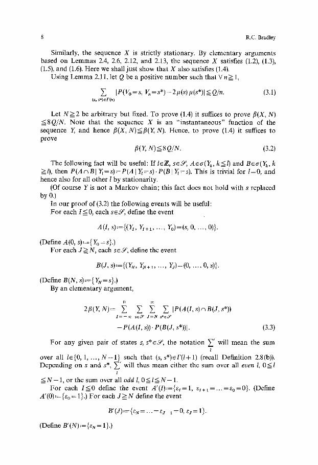
Similarly, the sequence X is strictly stationary. By elementary arguments based on Lemmas 2.4, 2.6, 2.12, and 2.13, the sequence X satisfies (1.2), (1.3), (1.5), and (1.6). Here we shall just show that X also satisfies (1.4).

Using Lemma 2.11, let Q be a positive number such that V n > 1,

IP(ro=s, g~=s*)-214s)#(s*)l~Q/n. (s, s * ) e r ( n )

(3.1)

Let N > 2 be arbitrary but fixed. To prove (1.4) it suffices to prove fi(X, N) <8Q/N. Note that the sequence X is an "instantaneous" function of the sequence Y, and hence fl(X, N)<fl(Y,N). Hence, to prove (1.4) it suffices to prove

fl(Y, N) < 8 Q/N. (3.2)

The following fact will be useful: If leTZ., se5 ~, Asa(Yk, k<l) and Bea(Yk, k >l), then P(A~BI Y~=s)=P(AI Yt=s).P(BI Yt=s). This is trivial for l=0 , and hence also for all other l by stationarity.

(Of course Y is not a Markov chain; this fact does not hold with s replaced by 0.)

In our proof of (3.2) the following events will be useful: For each I_< 0, each s e 5 ~, define the event

A(I, s),={(Y~, Y,+I, .- . , Y0)=(s, 0 . . . . ,0)}.

(Define A(0, s).'--{ Yo =s}.) For each J>=N, each s~5 e, define the event

B(J, s):={(Yu, Y N + I . . . . , Y j ) ~ - ( 0 , . . . , O, s)}.

(Define B(N, S),= { YN= S}. ) By an elementary argument,

2fl(Y, N)= 0

Z Z ~ E IP(A(I,s)nB(J,s*)) I = - - m s ~ 9 ~ J = N s*~5 a

-P(A(I , s)). P(B(J, s*))l. (3.3)

For any given pair of states s, s*eSf, the notation ~ ' will mean the sum z

over all le{0, 1, ..., N- - I} such that (s, s*)eF(l+l) (recall Definition 2.8(b)). Z' Depending on s and s*, will thus mean either the sum over all even l, O<l

< N - 1, or the sum over all odd l, 0 < l < N-- 1. For each 1 < 0 define the event A'(I).-={t~=l, ti+a . . . . . %=0}. (Define

A' (0),= {to = 1}.) For each J > N define the event

B'(J),={t u . . . . . ts_ 1 =0, is= 1}.

(Define B'(N),={eN = 1}.)

Sequence for which the CLT Fails 9

Define the r.v. Z :=el + . . . + ~N-1- Then by (3.3) and elementary calculations (and our stipulation N > 2),

0

2fl(Y,N)= Z Z Z Z I = - o o se~9 ~ J = N s * e ~

0

: Z Z 2 Z I = - - o o seS" J = N s * a ~

I~'; P(A(I, s)~B(J, s*)c~ { Z = / } ) l

-- P(A(I , s)). P(B(J, s*)). 2 ~ ' P ( Z = 1)[ l

IZ'P({ Vo = s} n A' (/) n {[7//+ 1 = S * } ("1 B' (J) c~ {Z = l} l

-- P(A'(I)) . p (s). P (B' (J))- p (s*). 2 ~ ' P (Z =/)l l

= ~ ~', ~, ~, I P (A'(I)). P (B' (J)). ~ ' P (Z = l) I s J s* l

�9 [P(Vo=s, Vz+l=s*)-2#(s)#(s*)]l

< Z P (A' (I)). Z P (B' (J)) . ~ Z ~ ' P (Z = l) I J s s* I

�9 IP(Vo=s, ~+,--s*)-2Ms)a(s*)l N - 1

=1-1. ~ ~ P(Z=I).IP(Vo=s, Vz+,=s*)-Zp(s)p(s*)l l = 0 ( s , s * ) ~ F ( l + 1)

N - - 1

~, P(Z=I). Q/(l+ 1) / = 0

P(Z N (N-- 1)/4). Q + P(Z > ( N - 1)/4) �9 4 Q/(N- 1)

4 Q/ (N- 1) + 4 Q/(N- 1) = 8 Q/(N- 1) =< 16 Q/N.

holds, and this completes the proof of (1.4). T h u s (3.2)

Acknowledgments. The author thanks R. Burton, who inspired this work; S. Janson for helpful com- ments and a preprint of [8]; and P. Ney for acquainting the author with Rogozin's [9] paper.

References

1. Bradley, R.C.: Counterexamples to the central limit theorem under strong mixing conditions. In: Revesz, P. (ed.). Colloquia mathematica societatis Janos Bolyai 36. Limit theorems in probabili- ty and statistics, Veszprem (Hungary), 1982, pp. 153-172. Amsterdam: North-Holland, 1985

2. Bradley, R.C.: On the central limit question under absolute regularity. Ann. Probab. 13, 1314-1325 (1985)

3. Bradley, R.C.: On some results of M.I. Gordin: a clarification of a misunderstanding. J. Theor. Probab. 1, 115-119 (1988)

4. Davydov, Yu.A.: Mixing conditions for Markov chains. Theory Probab. Appl. 18, 312-328 (1973) 5. Etemadi, N.: An elementary proof of the strong law of large numbers. Z. Wahrscheinlichkeitstheor.

Verw. Geb. 55, 119-122 (1981)

10 R.C. Bradley

6. Herrndorf, N.: Stationary strongly mixing sequences not satisfying the central limit theorem. Ann. Probab. 11, 809-813 (1983)

7. Ibragimov, I.A., Linnik, Yu.V.: Independent and stationary sequences of random variables. Gro- ningen: Wolters-Noordhoff, 1971

8. Janson, S.: Some pairwise independent sequences for which the central limit theorem fails. Stochas- tics 23, 439-448 (1988)

9. Rogozin, B.A.: An estimate of the remainder term in limit theorems of renewal theory. Theory Probab. Appl. 18, 662-677 (1973)

10. Volkonskii, V.A., Rozanov, Yu.A.: Some limit theorems for random functions I. Theory Probab. Appl. 4, 178-197 (1959)

11. Volkonskii, V.A., Rozanov, Yu.A.: Some limit theorems for random functions II. Theory Probab. Appl. 6, 186-198 (1961)

Received March 17, 1987; in revised form July 22, 1988