Agriculture, Ecosystems and Environment 81 (2000) 5–16

A spatial approach using imprecise soil data formodelling crop yields over vast areas

Philippe Lagacheriea,∗, Durk R. Cazemiera,Roger Martin-Clouaireb, Tom Wassenaara

a INRA Science du Sol, 2 Place Pierre Viala, 34060 Montpellier Cedex, Franceb INRA, Biométrie et Intelligence Artificielle, BP27, 31326 Castanet-Tolosan Cedex, France

Received 25 August 1999; received in revised form 10 December 1999; accepted 28 February 2000

Abstract

Estimations of crop yields using process-based crop models are area-limited because quantitative soil data are unavailableover vast areas. The spatial approach proposed in this study incorporates two novel aspects concerning the derivation ofsoil data feeding the simulation and the modelling of the crop production process. First, the soil parameters required forcrop modelling as well as their imprecision were estimated from the qualitative information of a 1:250,000 scale regional soildatabase by a possibility theory approach, which combines a set of GIS procedures and a constraint satisfaction solver. Second,the initial process-based crop model was made less complex by deriving simple agrotransfer functions from simulations atrepresentative sites located in the studied region. The resulting system estimated the yield expressed as possibility distributionsover the region which can be visualised through decision maps. The proposed spatial approach was tested on a hard wheatyield (Triticum durumspp.) estimation in the Hérault-Orb-Libron valley region (Languedoc, France). It proved to providerealistic yet imprecise estimates compared with those obtained for a set of site-crop estimates. The spatial approach allowedthe identification of areas in which soil data needed to be improved for obtaining both reliable and informative estimates. Theseresults demonstrated the potential usefulness of the proposed approach for providing reliable soil information for decisionmaking at the regional level. © 2000 Elsevier Science B.V. All rights reserved.

Keywords:Soil map; Available water capacity; Regional scale; Crop model; Imprecision; Possibility theory; Constraint satisfaction problem;GIS

1. Introduction

Computer simulations of soil water regimes andcrop growth are powerful means for quantifying theeffects of changing climate conditions or agriculturalpractices. However, these simulations require a largeamount of quantitative soil data which limits their spa-tial application to areas where a dense spatial sampling

∗ Corresponding author. Tel.:+33-4-99-61-25-78;fax: +33-4-67-63-26-14.

can be undertaken. A spatial approach is needed forextending the simulations to vast areas such as Euro-pean regions.

The common practice for doing this consists inlinking crop models to quantitative information pro-vided by soil maps and soil databases (Dumanski etal., 1993; Smaling and Fresco, 1993; Akinremi et al.,1997; Bornand et al., 1998). This type of informa-tion consists in measured soil data from detailed soilprofile observations that are assumed to be represen-tative for the delineated mapping units. Crop yield

0167-8809/00/$ – see front matter © 2000 Elsevier Science B.V. All rights reserved.PII: S0167-8809(00)00164-X

6 P. Lagacherie et al. / Agriculture, Ecosystems and Environment 81 (2000) 5–16

simulations can then be undertaken by using theseinput data, if necessary, in combination with pedo-transfer functions (Bouma and van Lanen, 1987). Theso obtained results are assumed to be valid for thewhole mapping unit, thus allowing easy mapping byclassical GIS procedures.

This straightforward approach becomes question-able when yield must be mapped over large areas.Generally, small scale soil maps (<1:250,000) arethe only available soil information over such areas.At this scale the mapping units often include severaltaxonomic units, each of them characterised by a rep-resentative profile. The common practice is to selectthe representative profile of the dominant taxonomicunits which can lead to neglect a substantial part ofthe mapping unit area (Le Bas et al., 1998). Further-more the taxonomic units of a small scale soil mapcannot be reduced to the description of a unique setof parameters measured at a given site because of itshigh within-unit variability. Resuming, the exclusiveuse of quantitative information derived from a smallscale soil map leads to a misrepresentation of the soilvariability of the region. This may have consequenceson yield mapping and further decision making.

A possible alternative is to use the qualitative de-scription of the soil taxonomic units (STUs) of asmall scale map as input data for crop models. Thisdescription provides a more synthetic understandingof the taxonomic units taking into account the entireinformation collected by the soil surveyor in the field,i.e. soil profiles, auger hole observations and surfacefeatures observations. The description of a STU alsoincludes a description of environmental attributes(e.g. geology, land use, slope). If maps of these at-tributes exist for the studied region, the environmentaldescriptions can be used for estimating the locationof each STU within the complex soil mapping unitsof the 1:250,000 scale soil map.

All this qualitative information, generally based onwell-established codification systems (FAO-UNESCO,1981; Baize and Jabiol, 1995), is now easily avail-able in soil databases (Oldeman and van Engelen,1993; Bornand et al., 1994; King et al., 1994). Thisinformation is, however, still underexploited in yieldpredictions. The approach presented below estimatescrop yields over a region by coupling simulationswith the qualitative descriptions of taxonomic soilunits of a 1:250,000 soil database. Such coupling is

made through agrotransfer functions derived from aset of crop model simulations undertaken over a setof representative soil climate situations. The proposedapproach uses possibility theory for representing andhandling the required qualitative information. It wasapplied within the framework of the EC funded re-search project IMPEL (Rounsevell et al., 1998) formapping hard wheat yields evolutions with changingclimate conditions over a region of 1200 km2 locatedin the Languedoc plain (southern France). This paperfocuses on the estimation of wheat yield under actualclimate conditions. The climate changes issues dealtin the IMPEL project are detailed in Wassenaar et al.(1999).

2. The spatial approach

2.1. Representing qualitative descriptions of soiltaxonomic units by possibility distributions

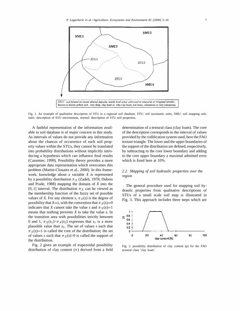
Fig. 1 shows an example of description of STUin a regional soil database. STUs are non-geographiccomponents of soil landscape units (King et al., 1994)delineated in small scale soil maps. The first part ofSTU description (Fig. 1, in italics) deals with the STUenvironment whereas the second part is a descriptionof the soil properties which characterise the STU.

A soil or environment attribute qualifying a STU isexpressed by a categorical variable corresponding toa range of values according to a coding system. Forexample, the soil texture class ‘clay loam’, definedin the texture triangle, corresponds to three intervalsof values for the clay, silt and sand content. Thismeans precisely that if a STU is described as ‘clayloam’ then, (1) all the clay silt and sand content val-ues included in the intervals defining ‘clay loam’ canbe encountered within the STU, (2) nothing can besaid about the respective chances of occurrence ofany of the individual values included in the intervals.However, clay, silt and sand content values slightlyinferior to the lower clay loam intervals limits, orslightly superior to the upper ones, cannot be totallyrejected since textural classes are subjective estima-tions prone to errors and imprecisions. The qualitativedescription of a STU should, therefore, be expressedby a set of intervals of values bounded by fuzzylimits.

P. Lagacherie et al. / Agriculture, Ecosystems and Environment 81 (2000) 5–16 7

Fig. 1. An example of qualitative description of STU in a regional soil database. STU: soil taxonomic units, SMU: soil mapping unit,italic: description of STU environment, normal: description of STU soil properties.

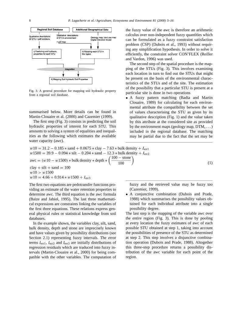
A faithful representation of the information avail-able in soil database is of major concern in this study.As intervals of values do not provide any informationabout the chances of occurrence of each soil prop-erty values within the STUs, they cannot be translatedinto probability distributions without implicitly intro-ducing a hypothesis which can influence final results(Cazemier, 1999). Possibility theory provides a moreappropriate data representation which overcomes thisproblem (Martin-Clouaire et al., 2000). In this frame-work, knowledge about a variableX is representedby a possibility distributionπX (Zadeh, 1978; Duboisand Prade, 1988) mapping the domain ofX into the[0, 1] interval. The distributionπX can be viewed asthe membership function of the fuzzy set of possiblevalues ofX. For any elements, πX(s) is the degree ofpossibility thatX=s, with the convention thatπX(s)=0indicates thatX cannot take the values andπX(s)=1means that nothing preventsX to take the values. Inthe transition area with possibilities strictly between0 and 1,πX(s1)>πX(s2) expresses thats1 is a moreplausible value thans2. The set of valuess such thatπX(s)=1 is called the core of the distribution; the setof valuess such thatπX(s)>0 is called the support ofthe distribution.

Fig. 2 gives an example of trapezoidal possibilitydistribution of clay content (π ) derived from a field

determination of a textural class (clay loam). The coreof the description corresponds to the interval of valuesprovided by the codification system used, here the FAOtexture triangle. The lower and the upper boundaries ofthe support of the distribution are defined, respectively,by subtracting to the core lower boundary and addingto the core upper boundary a maximal admitted errorwhich is fixed here at 10%.

2.2. Mapping of soil hydraulic properties over theregion

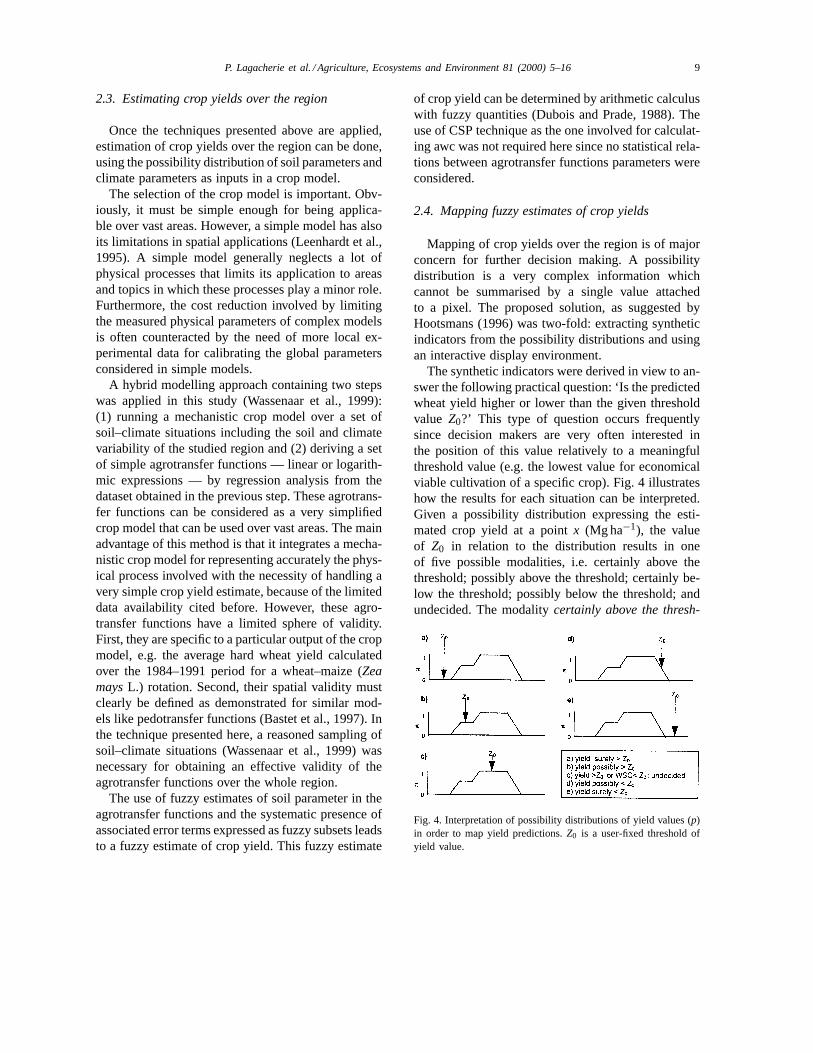
The general procedure used for mapping soil hy-draulic properties from qualitative descriptions ofSTUs of a small scale soil map is illustrated inFig. 3. This approach includes three steps which are

Fig. 2. possibility distribution of clay content (p) for the FAOtextural class ‘clay loam’.

8 P. Lagacherie et al. / Agriculture, Ecosystems and Environment 81 (2000) 5–16

Fig. 3. A general procedure for mapping soil hydraulic propertyfrom a regional soil database.

summarised below. More details can be found inMartin-Clouaire et al. (2000) and Cazemier (1999).

The first step (Fig. 3) consists in predicting the soilhydraulic properties of interest for each STU. Thisamounts to solving a system of equalities and inequal-ities as the following which estimates the availablewater capacity (awc).

w10 = 31.2 − 0.185∗ sand+ 0.0675∗ clay− 7.63∗ bulk density+ Ierr1w1500= 39.9 − 0.094∗ silt − 0.204∗ sand− 12.3 ∗ bulk density+ Ierr2

awc= (w10− w1500) ∗ bulk density∗ depth∗(

100− stone

100

)

clay+ silt + sand= 100w10 > w1500w10 = 4.66+ 0.914∗ w1500+ Ierr3

(1)

The first two equations are pedotransfer functions pro-viding an estimate of the water retention properties todetermine awc. The third equation is the awc formula(Baize and Jabiol, 1995). The last three mathemati-cal expressions are constraints linking the variables ofthe first three equations. These relations express gen-eral physical rules or statistical knowledge from soildatabases.

In the example shown, the variables clay, silt, sand,bulk density, depth and stone are imprecisely knownand have values given by possibility distributions (seeSection 2.1) representing fuzzy intervals. The errortermsIerr1, Ierr2 and Ierr3 are initially distributions ofregression residuals which are traduced into fuzzy in-tervals (Martin-Clouaire et al., 2000) for being com-patible with the other variables. The computation of

the fuzzy value of the awc is therefore an arithmeticcalculus over non-independent fuzzy quantities whichcan be formulated as a fuzzy constraint satisfactionproblem (CSP) (Dubois et al., 1993) without requir-ing any simplification hypothesis. In order to solve itefficiently, the constraint solver CON’FLEX (Reillerand Vardon, 1996) was used.

The second step of the spatial procedure is the map-ping of the STUs (Fig. 3). This involves examiningeach location in turn to find out the STUs that mightbe present on the basis of the environmental charac-teristics of the STUs and of the site. The estimationof the possibility that a particular STU is present at aparticular site is done in two operations• A fuzzy pattern matching (Badia and Martin

Clouaire, 1989) for calculating for each environ-mental attribute the compatibility between the setof values characterising the STU as given by itsqualitative description (Fig. 1) and the value takenby this attribute at the considered site as providedby the environment maps (geology map, DTM,. . . )included in the regional database. The matchingmay be partial due to the fact that the set may be

fuzzy and the retrieved value may be fuzzy too(Cazemier, 1999).

• A conjunctive combination (Dubois and Prade,1988) which summarises the possibility values ob-tained for each individual attribute into a singlepossibility degree.

The last step is the mapping of the variable awc overthe entire region (Fig. 3). This is done by poolingat every location the fuzzy estimates of awc of eachpossible STU obtained at step 1, taking into accountthe possibilities of presence of the STU as determinedat step 2. This step involves a disjunctive combina-tion operation (Dubois and Prade, 1988). Altogetherthis three-step procedure returns a possibility dis-tribution of the awc variable for each point of theregion.

P. Lagacherie et al. / Agriculture, Ecosystems and Environment 81 (2000) 5–16 9

2.3. Estimating crop yields over the region

Once the techniques presented above are applied,estimation of crop yields over the region can be done,using the possibility distribution of soil parameters andclimate parameters as inputs in a crop model.

The selection of the crop model is important. Obv-iously, it must be simple enough for being applica-ble over vast areas. However, a simple model has alsoits limitations in spatial applications (Leenhardt et al.,1995). A simple model generally neglects a lot ofphysical processes that limits its application to areasand topics in which these processes play a minor role.Furthermore, the cost reduction involved by limitingthe measured physical parameters of complex modelsis often counteracted by the need of more local ex-perimental data for calibrating the global parametersconsidered in simple models.

A hybrid modelling approach containing two stepswas applied in this study (Wassenaar et al., 1999):(1) running a mechanistic crop model over a set ofsoil–climate situations including the soil and climatevariability of the studied region and (2) deriving a setof simple agrotransfer functions — linear or logarith-mic expressions — by regression analysis from thedataset obtained in the previous step. These agrotrans-fer functions can be considered as a very simplifiedcrop model that can be used over vast areas. The mainadvantage of this method is that it integrates a mecha-nistic crop model for representing accurately the phys-ical process involved with the necessity of handling avery simple crop yield estimate, because of the limiteddata availability cited before. However, these agro-transfer functions have a limited sphere of validity.First, they are specific to a particular output of the cropmodel, e.g. the average hard wheat yield calculatedover the 1984–1991 period for a wheat–maize (ZeamaysL.) rotation. Second, their spatial validity mustclearly be defined as demonstrated for similar mod-els like pedotransfer functions (Bastet et al., 1997). Inthe technique presented here, a reasoned sampling ofsoil–climate situations (Wassenaar et al., 1999) wasnecessary for obtaining an effective validity of theagrotransfer functions over the whole region.

The use of fuzzy estimates of soil parameter in theagrotransfer functions and the systematic presence ofassociated error terms expressed as fuzzy subsets leadsto a fuzzy estimate of crop yield. This fuzzy estimate

of crop yield can be determined by arithmetic calculuswith fuzzy quantities (Dubois and Prade, 1988). Theuse of CSP technique as the one involved for calculat-ing awc was not required here since no statistical rela-tions between agrotransfer functions parameters wereconsidered.

2.4. Mapping fuzzy estimates of crop yields

Mapping of crop yields over the region is of majorconcern for further decision making. A possibilitydistribution is a very complex information whichcannot be summarised by a single value attachedto a pixel. The proposed solution, as suggested byHootsmans (1996) was two-fold: extracting syntheticindicators from the possibility distributions and usingan interactive display environment.

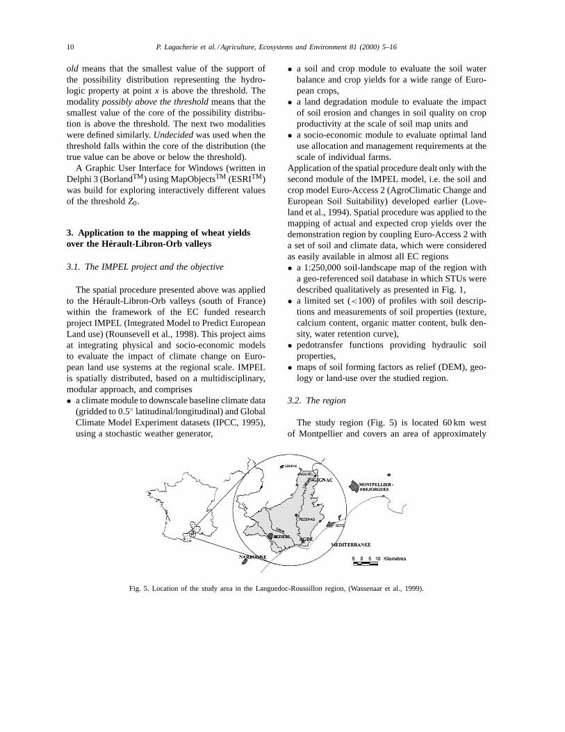
The synthetic indicators were derived in view to an-swer the following practical question: ‘Is the predictedwheat yield higher or lower than the given thresholdvalue Z0?’ This type of question occurs frequentlysince decision makers are very often interested inthe position of this value relatively to a meaningfulthreshold value (e.g. the lowest value for economicalviable cultivation of a specific crop). Fig. 4 illustrateshow the results for each situation can be interpreted.Given a possibility distribution expressing the esti-mated crop yield at a pointx (Mg ha−1), the valueof Z0 in relation to the distribution results in oneof five possible modalities, i.e. certainly above thethreshold; possibly above the threshold; certainly be-low the threshold; possibly below the threshold; andundecided. The modalitycertainly above the thresh-

Fig. 4. Interpretation of possibility distributions of yield values (p)in order to map yield predictions.Z0 is a user-fixed threshold ofyield value.

10 P. Lagacherie et al. / Agriculture, Ecosystems and Environment 81 (2000) 5–16

old means that the smallest value of the support ofthe possibility distribution representing the hydro-logic property at pointx is above the threshold. Themodality possibly above the thresholdmeans that thesmallest value of the core of the possibility distribu-tion is above the threshold. The next two modalitieswere defined similarly.Undecidedwas used when thethreshold falls within the core of the distribution (thetrue value can be above or below the threshold).

A Graphic User Interface for Windows (written inDelphi 3 (BorlandTM) using MapObjectsTM (ESRITM)was build for exploring interactively different valuesof the thresholdZ0.

3. Application to the mapping of wheat yieldsover the Hérault-Libron-Orb valleys

3.1. The IMPEL project and the objective

The spatial procedure presented above was appliedto the Hérault-Libron-Orb valleys (south of France)within the framework of the EC funded researchproject IMPEL (Integrated Model to Predict EuropeanLand use) (Rounsevell et al., 1998). This project aimsat integrating physical and socio-economic modelsto evaluate the impact of climate change on Euro-pean land use systems at the regional scale. IMPELis spatially distributed, based on a multidisciplinary,modular approach, and comprises• a climate module to downscale baseline climate data

(gridded to 0.5◦ latitudinal/longitudinal) and GlobalClimate Model Experiment datasets (IPCC, 1995),using a stochastic weather generator,

Fig. 5. Location of the study area in the Languedoc-Roussillon region, (Wassenaar et al., 1999).

• a soil and crop module to evaluate the soil waterbalance and crop yields for a wide range of Euro-pean crops,

• a land degradation module to evaluate the impactof soil erosion and changes in soil quality on cropproductivity at the scale of soil map units and

• a socio-economic module to evaluate optimal landuse allocation and management requirements at thescale of individual farms.

Application of the spatial procedure dealt only with thesecond module of the IMPEL model, i.e. the soil andcrop model Euro-Access 2 (AgroClimatic Change andEuropean Soil Suitability) developed earlier (Love-land et al., 1994). Spatial procedure was applied to themapping of actual and expected crop yields over thedemonstration region by coupling Euro-Access 2 witha set of soil and climate data, which were consideredas easily available in almost all EC regions• a 1:250,000 soil-landscape map of the region with

a geo-referenced soil database in which STUs weredescribed qualitatively as presented in Fig. 1,

• a limited set (<100) of profiles with soil descrip-tions and measurements of soil properties (texture,calcium content, organic matter content, bulk den-sity, water retention curve),

• pedotransfer functions providing hydraulic soilproperties,

• maps of soil forming factors as relief (DEM), geo-logy or land-use over the studied region.

3.2. The region

The study region (Fig. 5) is located 60 km westof Montpellier and covers an area of approximately

P. Lagacherie et al. / Agriculture, Ecosystems and Environment 81 (2000) 5–16 11

1200 km2. The region exhibits typical northernMediterranean climate characteristics, i.e. a substan-tial average annual rainfall (on average 700 mm peryear), a high within-year rainfall variability with rain-fall peaks in autumn and spring and strong droughtsin summer, high between-year rainfall variability,frequent and violent rainstorms and a large potentialevapotranspiration (PET) (on average 1000 mm peryear) due to the high average temperature and radia-tion and frequent and strong winds. The temperatureexhibits only small variations across the studied re-gion (annual minimal temperature ranging from 8.7to 10.1◦C, annual maximal temperature from 19.1to 19.6◦C). Conversely, the weather stations withinthe region reveal a strong within-region-variabilityregarding rainfall (570–810 mm), which demonstratesa clear south–north gradient. PET measurements areonly available from two weather stations, Narbonneand Montpellier-Fréjorgues which are situated at ei-ther side of the region (Fig. 5). The difference in an-nual average PET registered at both weather stationsdoes not exceed 6%.

The regional soil pattern is extremely complexmainly due to the large geological variations. The ba-sic substratum is an heterogeneous Miocene marinesediment on which either Lithic Leptosols, CalcaricRegosols or Calcaric Cambisols (FAO-UNESCO,1981) have formed. This substratum is partiallyoverlain by Pleistocene alluvial deposits. These de-posits have produced stony soils ranging from Cal-caric to Chromic Luvisols. The most recent alluvial(Holocene) deposits contain Calcaric Fluvisols. Lo-cal volcanic activity and recent colluvial phenom-ena have contributed to the soil heterogeneity. Thesoil-landscape map of the studied region at 1:250,000(Bornand et al., 1994) defines 36 soil-landscape unitsincluding 96 STUs in total.

3.3. Mapping hard wheat yields over the region

3.3.1. Deriving agrotransfer functions from a set oftypical soil–climate situations

A limited number of simulation sites were selectedin order to take into account the soil and climate vari-ability of the region (Wassenaar et al., 1999). Sixty-three soil profiles located within or at the vicin-ity of the study region were extracted from theLanguedoc-Roussillon soil database (Bornand et al.,

1994) providing each of them the required input datafor the Euro-Access model. The total set of profilesrepresented the range of soil types that occur in theregion in terms of their hydraulic behaviour (Bornandet al., 1992; Bonfils, 1993).

Climate variability of the region was consideredthrough a set of theoretical weather stations definedby assembling daily input data from available stationslocated within and near the study region. As stated inthe previous section, temperature and PET exhibit onlyslight variations throughout the region, which allowsthe use of a unique data set of daily parameters, i.e.the one of the Montpellier-Fréjorgues weather station.Three weather stations, Béziers, Pézenas and Aniane,were selected to represent the south–north gradient as-sociated with change in elevation as this is the onlynoticeable climatic trend affecting the region.

The 63 soil profiles were combined with the threeselected weather stations to obtain 189 theoreticalsoil–climate situations representing the range of soil–climate spatial variations observed within the region.The simulations were made using the crop modelEuro-Access 2. A detailed description of the modeland of the calibration protocol is provided in Wasse-naar et al. (1999).

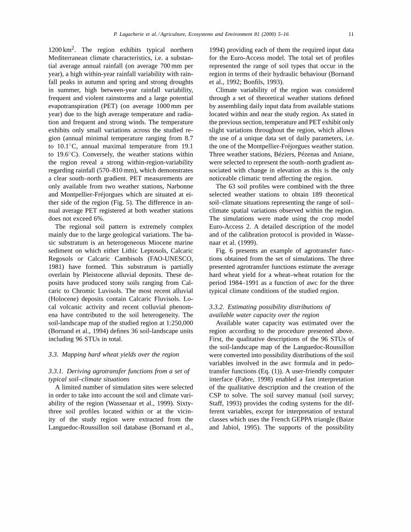
Fig. 6 presents an example of agrotransfer func-tions obtained from the set of simulations. The threepresented agrotransfer functions estimate the averagehard wheat yield for a wheat–wheat rotation for theperiod 1984–1991 as a function of awc for the threetypical climate conditions of the studied region.

3.3.2. Estimating possibility distributions ofavailable water capacity over the region

Available water capacity was estimated over theregion according to the procedure presented above.First, the qualitative descriptions of the 96 STUs ofthe soil-landscape map of the Languedoc-Roussillonwere converted into possibility distributions of the soilvariables involved in the awc formula and in pedo-transfer functions (Eq. (1)). A user-friendly computerinterface (Fabre, 1998) enabled a fast interpretationof the qualitative description and the creation of theCSP to solve. The soil survey manual (soil survey;Staff, 1993) provides the coding systems for the dif-ferent variables, except for interpretation of texturalclasses which uses the French GEPPA triangle (Baizeand Jabiol, 1995). The supports of the possibility

12 P. Lagacherie et al. / Agriculture, Ecosystems and Environment 81 (2000) 5–16

Fig. 6. Estimations of mean hard wheat yield over the period 1984-1991 for three representative climate situations (Beziers, Aniane,Pezenas), as a function of the soil awc. Correlation coefficients of curves fitted to the data are shown on the graph (Wassenaar et al., 1999).

distributions were defined according to the maximumadmitted errors (Table 1). The qualitative descriptionsof STUs do not include any information about thebulk density of the soil. Consequently, a unique pos-sibility distribution was defined for the region froma set of soil bulk density measurements. The coreand the support of this distribution are given by theintervals (1.35, 1.60) and (1.15, 1.85), respectively.

Second, awc was mapped over the region follow-ing the scheme presented in Fig. 3. Available watercapacities of the 96 STUs were determined accord-ing to Section 2.2. The points of the water retentioncurve involved in expressing awc were estimated bypedotransfer functions derived from dataset containing372 measurements of hydraulic properties of soil hori-zons located in the Languedoc-Roussillon (Bastet etal., 1997). Different pedotransfer functions were cal-culated for four classes of substratum to increase the

Table 1The maximum errors used for defining supports of possibilitydistributions

Variable Maximum error

Clay, silt, sand 100 g kg−1

Depth 10 cmStoniness 100 g kg−1

Organic matter content 10 g kg−1 (lower classes)50 g kg−1 (upper classes)

Slope gradient 2 cm m−1 (lower classes)5 cm m−1 (upper classes)

precision of estimations. A similar technique was ap-plied to determine the relation between the two pointsof the retention curve (last equation of system (1)).For each of these statistical relations, the error termwas converted into possibility distributions. As statedin Section 2.2.1, the CSP solver CON’FLEX was usedfor calculating the final possibility distribution of awcper STU.

The presence of STUs was determined in terms ofpossibility at each node of a 100 m×100 m grid cov-ering the region according to Section 2.2. Additionalgeographical information involved in this step was asfollows: (1) a slope gradient map derived from digi-tal elevation model at scale 1:25,000; (2) a 1:50,000geological map and (3) a land use map derived fromthe 1:25,000 topographical map. The error terms as-sociated with (1) and the positional uncertainty ofthe boundaries of the map units of (2) and (3) weredetermined statistically by comparing with more pre-cise information which was available in some limitedareas in the region like air-photograph-derived DEM,detailed soil maps (Cazemier, 1999). The possibil-ity theory algorithms required for calculating thepossibility of presence of STUs (Section 2.2) wereimplemented in the macro language of Arc/InfoTM.

Finally, distributions of possibility of awc were ob-tained over the region by merging the two previoussteps according to the disjunctive combination oper-ation mentioned in Section 1.2. This algorithm wasalso implemented in the Arc/InfoTM macro-language.

P. Lagacherie et al. / Agriculture, Ecosystems and Environment 81 (2000) 5–16 13

3.3.3. Applying agrotransfer functions with fuzzyestimates of available water capacity

The application of the agrotransfer functionsamounts to a fuzzy calculus as presented in Section2.3. Prior to this, each node of the grid covering theregion was allocated to one of the three consideredtypical climate situations in view to select the adequateagrotransfer function. This was done by a nearest-neighbour algorithm. All these operations were per-formed within the GIS Arc/InfoTM.

3.4. Results and discussion

The evaluation of the estimates of awc by the pro-posed spatial procedure addressed two questions: (1)do the estimates match reality?, and (2) are they in-formative?

To answer the first question, a validation set of 111sites with measured Euro-Access 2 soil inputs wasconsidered in the study region. At each site, a meanannual wheat yield for the period 1984–1991 was cal-culated by an Euro-Access 2 simulation. To use thesevalidation data for evaluating the spatial procedure,the estimated possibility distributions of wheat yieldwere first traduced into a set of crisp prediction inter-vals each defined by the two values of yield having agiven possibility level (Fig. 7). The prediction inter-vals were then evaluated at each site by determiningwhether they include or not the calculated yields.Finally prediction errors were defined for each pos-sibility level by calculating over the set of validationsites the percentage of wrong predictions provided byintervals defined at the considered possibility level.

Fig. 8 shows the prediction errors calculated fromthe different levels of possibility. It reveals that the

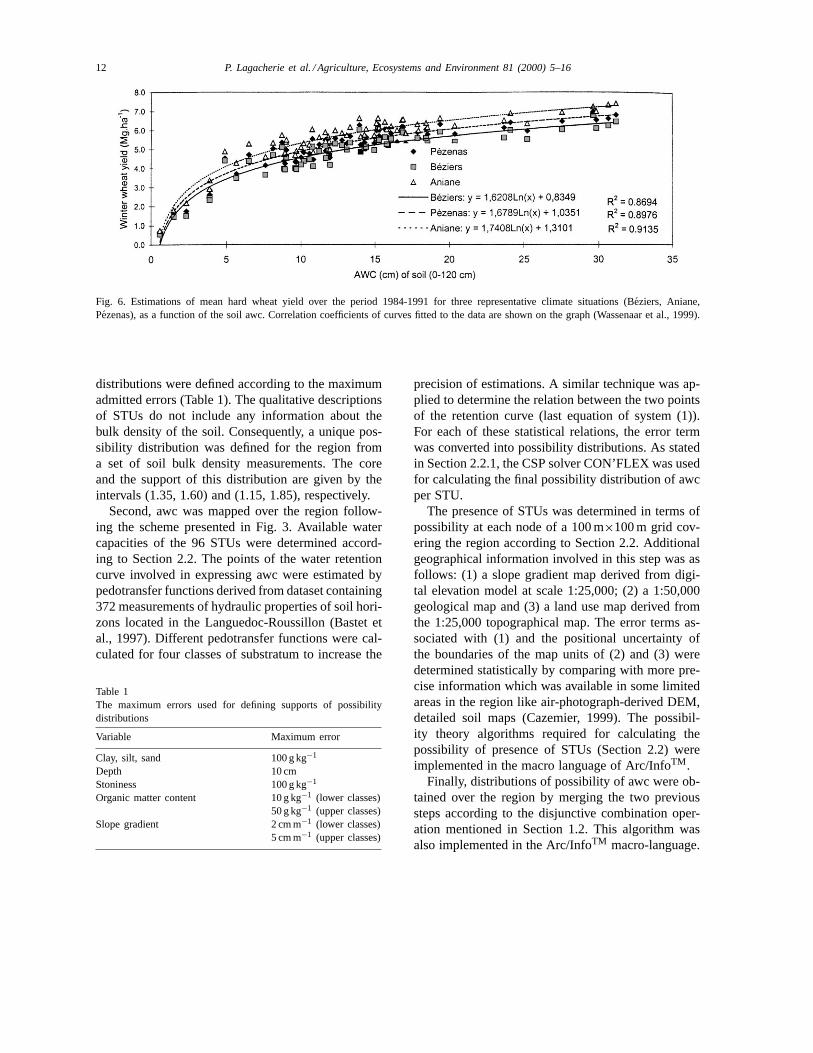
Fig. 7. The definition of prediction intervals (black arrows) forpossibility levels 0.1, 0.5 and 1 from estimated possibility distri-bution of yields (grey line).

Fig. 8. Prediction errors of yield estimates according to possibilitylevels p at which are defined prediction intervals.

proposed spatial procedure provided very reliableestimates since the error was never higher than 12%(possibility level=1). For possibility levels lowerthan 0.8, the predicted points were all included in theprediction intervals.

To determine whether the predictions are infor-mative or not, the widths of the prediction intervalsderived from the estimated possibility distributionscalculated over the whole region were considered.The larger the interval is, the less informative the pre-diction. For example, predicting that wheat yield isin the interval 3.5–4.8 Mg ha−1, is more informativethan predicting yield in the interval 1.5–4.8 Mg ha−1.

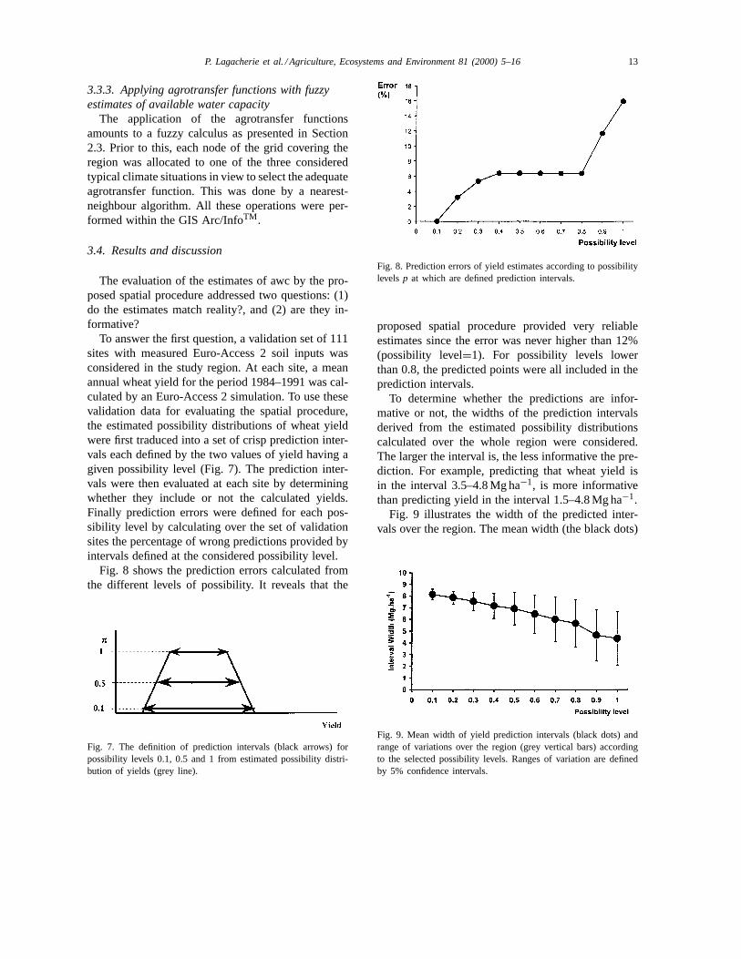
Fig. 9 illustrates the width of the predicted inter-vals over the region. The mean width (the black dots)

Fig. 9. Mean width of yield prediction intervals (black dots) andrange of variations over the region (grey vertical bars) accordingto the selected possibility levels. Ranges of variation are definedby 5% confidence intervals.

14 P. Lagacherie et al. / Agriculture, Ecosystems and Environment 81 (2000) 5–16

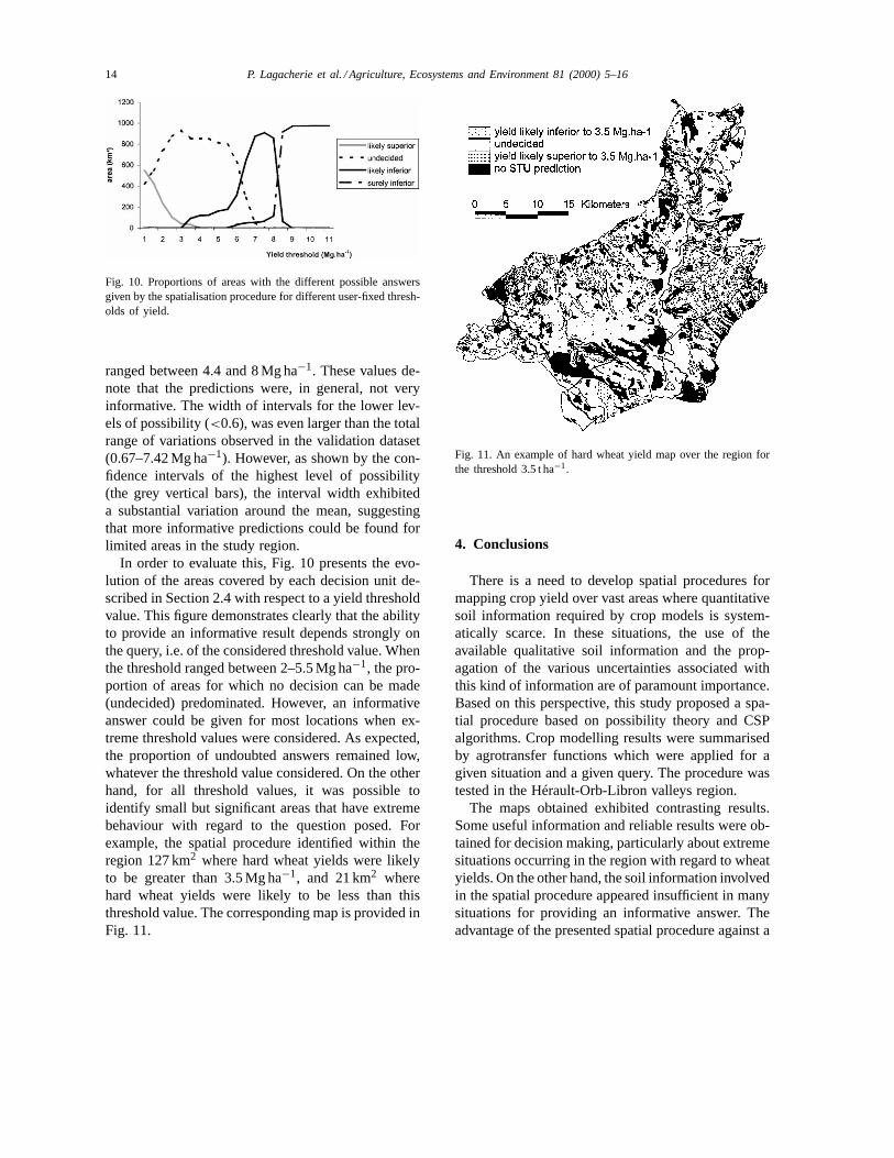
Fig. 10. Proportions of areas with the different possible answersgiven by the spatialisation procedure for different user-fixed thresh-olds of yield.

ranged between 4.4 and 8 Mg ha−1. These values de-note that the predictions were, in general, not veryinformative. The width of intervals for the lower lev-els of possibility (<0.6), was even larger than the totalrange of variations observed in the validation dataset(0.67–7.42 Mg ha−1). However, as shown by the con-fidence intervals of the highest level of possibility(the grey vertical bars), the interval width exhibiteda substantial variation around the mean, suggestingthat more informative predictions could be found forlimited areas in the study region.

In order to evaluate this, Fig. 10 presents the evo-lution of the areas covered by each decision unit de-scribed in Section 2.4 with respect to a yield thresholdvalue. This figure demonstrates clearly that the abilityto provide an informative result depends strongly onthe query, i.e. of the considered threshold value. Whenthe threshold ranged between 2–5.5 Mg ha−1, the pro-portion of areas for which no decision can be made(undecided) predominated. However, an informativeanswer could be given for most locations when ex-treme threshold values were considered. As expected,the proportion of undoubted answers remained low,whatever the threshold value considered. On the otherhand, for all threshold values, it was possible toidentify small but significant areas that have extremebehaviour with regard to the question posed. Forexample, the spatial procedure identified within theregion 127 km2 where hard wheat yields were likelyto be greater than 3.5 Mg ha−1, and 21 km2 wherehard wheat yields were likely to be less than thisthreshold value. The corresponding map is provided inFig. 11.

Fig. 11. An example of hard wheat yield map over the region forthe threshold 3.5 t ha−1.

4. Conclusions

There is a need to develop spatial procedures formapping crop yield over vast areas where quantitativesoil information required by crop models is system-atically scarce. In these situations, the use of theavailable qualitative soil information and the prop-agation of the various uncertainties associated withthis kind of information are of paramount importance.Based on this perspective, this study proposed a spa-tial procedure based on possibility theory and CSPalgorithms. Crop modelling results were summarisedby agrotransfer functions which were applied for agiven situation and a given query. The procedure wastested in the Hérault-Orb-Libron valleys region.

The maps obtained exhibited contrasting results.Some useful information and reliable results were ob-tained for decision making, particularly about extremesituations occurring in the region with regard to wheatyields. On the other hand, the soil information involvedin the spatial procedure appeared insufficient in manysituations for providing an informative answer. Theadvantage of the presented spatial procedure against a

P. Lagacherie et al. / Agriculture, Ecosystems and Environment 81 (2000) 5–16 15

classical mapping was to identify the queries and theareas for which no information can be reasonably de-livered. However, the validation results suggested thatmore informative estimates could be obtained with thesame source data by modifying the parametrisationof the possibility distributions derived from the soildatabase. In the current situation, the range of reallyuseful possibility levels at which estimates are deliv-ered was very small since below possibility level 0.6,the estimates do not bring any information about thepossible values of yields. Since the prediction errorswere shown to be very low, higher risk can be acceptedwhen interpreting the input soil data — i.e. to reducethe width of both core and support of the possibilitydistributions — which can lead to more informativeestimates. This would be easier if a better knowledgeof the uncertainty associated with the soil data couldbe collected in regional databases.

In any case, this case study demonstrated that asignificant effort must be made for increasing the pre-cision of yield estimates over vast areas. Several pos-sible improvements of the existing soil databases canbe envisaged such as extending the range of system-atic soil characterisation (e.g. bulk density), derivingmore precise pedotransfer functions, providing moreaccurate descriptions of STUs (e.g. by means of rangeof values by soil horizons), and enlarging the mappingscale in view to locate the STU. To define prioritiesamong all these possible improvements requires acost-utility analysis which should take into accountthe variety of situations of a given region. The pro-cedure presented in this paper could be useful in thisperspective.

Acknowledgements

The research reported in this article was under-taken within the IMPEL project, and funded by theEuropean Commission under the Climate and En-vironment Programme of Framework IV (Contractno. ENV4-CT95-0114). The authors thank Dr. MarkRounsevell (University of Catholique de Louvain) forleading the IMPEL project. The authors also thankJ.P. Barthès, Dr. M. Bornand and P. Falipou for pro-viding the soil data used in the study and Alfred Steinfor his useful comments and corrections on an earlierversion of the manuscript.

References

Akinremi, O.O., McGinn, S.M., Howard, A.E., 1997. Regionalsimulation of fall and spring soil moisture in Alberta. Can. J.Soil Sci. 77, 431–442.

Badia, J., Martin Clouaire, R., 1989. Choice under imprecision:a simple possibility-theory-based technique illustrated with aproblem of weed identification. Comput. Electron. Agric. 4,103–120.

Baize, D., Jabiol, B., 1995. Guide pour la description des sols,INRA, Versailles.

Bastet, G., Bruand, A., Voltz, M., Bornand, M., Quétin, P., 1997.Performance of available pedotransfer function for predictingthe water retention properties of French soils. In: Proceedings ofthe International Workshop on New Developments in Estimatingthe Hydraulic Properties of Unsaturated Soils, Riverside, CA,USA.

Bonfils, P., 1993. Carte pédologique de France à 1/100 000. Feuillede Lodève, SESCPF INRA, Orléans.

Bornand, M., Barthès, J.P., Bonfils, P., 1992. Carte despédopaysages du Languedoc Roussillon à l’ échelle du1/250 000. Laboratoire de Science du Sol, Montpellier.

Bornand, M., de Laroche, E., Legros, J.P., 1998. Soil waterbalance of the vineyard of the Languedoc: a tool for rural areamanagement. In: Proceedings of the XVIth World Congress ofSoil Science, Montpellier, France.

Bornand, M., Legros, J.P., Rouzet, C., 1994. Les banquesrégionales de données-sols. Exemple du Languedoc-Roussillon.Etude et Gestion des Sols 1, 67–82.

Bouma, J., van Lanen, J.A.J., 1987. Transfert functions andthreshold values: From soil characteristics to land qualities.In: Beek, K.J., Burrough, P.A., McCormack, D.E. (Eds.),Proceedings of the ISSS and SSSA International workshop onQuantified Land Evaluation, ITC no. 6, Washington DC, USA.

Cazemier, D., 1999. Utilisation de l’information incertaine dérivéed’une base de données sols. Application à la cartographiedes propriétés hydriques à l’échelle régionale. Thèse Doctorat,Ecole Nationale Supérieure Agronomique, Montpellier.

Dubois, D., Prade, H., 1988. Possibility Theory: An Approach toComputerized Processing of Uncertainty, Plenum Press, NewYork.

Dubois, D., Fargier, H., Prade, H., 1993. Propagation andsatisfaction of fuzzy constraints. In: Yager, R., Zadeh, L. (Eds.),Fuzzy Sets, Neural Network and Soft Computing. KluwerAcademic Publishers, Dordrecht, pp. 166–187.

Dumanski, J., Pettapierce, W.W., Acton, D.F., Claude, P.P., 1993.Application of agro-ecological concepts and hierarchy theory inthe design of databases for spatial and temporal characterisationof land and soil. Geoderma 60, 343–358.

Fabre, J.C., 1998. Interface d’utilisation d’un résolveur decontraintes floues à l’usage d’un Agronome (CAPRISI), USTL,CNIAM, Montpellier.

FAO-UNESCO, 1981. Soil Map of the World at 1: 5,000,000.Food and Agriculture Organisation, Rome.

Hootsmans, R.M., 1996. Fuzzy sets and series analysis for visualdecision support in spatial data exploration. Ph.D. thesis,Utrecht University.

16 P. Lagacherie et al. / Agriculture, Ecosystems and Environment 81 (2000) 5–16

IPCC, 1995. Climate Change 1995: The Science of ClimateChange. Cambridge University Press, Cambridge.

King, D., Daroussin, J., Tavernier, R., 1994. Development of asoil geographic database from the soil map of the Europeancommunities. Catena 21, 37–56.

Le Bas, C., King, D., Daroussin, J., Nicoullaud, B., Ngongo,M., 1998. Impact of errors in the assessment of agronomicconstraints to crop production at a European scale. In:Proceedings of the XVIth World Congress of Soil Science,Montpellier, France.

Leenhardt, D., Voltz, M., Rambal, S., 1995. Survey of severalagroclimatic soil water balance models with reference to theirspatial application. Eur. J. Agron. 4, 1–14.

Loveland, P.J., Legros, J.P., Rounsevell, M.D.A., de la Rosa, D.,Armstrong, A., 1994. A spatially distributed soil agroclimaticand soil hydrological model to predict the effects of climatechange within the European community. In: Proceedings of theXV World Congress of Soil Science, Vol. 6a, Commission V,Acapulco, Mexico, pp. 83–100.

Martin-Clouaire, R., Cazemier, D., Lagacherie, P., 2000.Representing and processing uncertain soil information formapping hydrological soil properties. Computer & Electronicsin Agriculture, in press.

Oldeman, L.R., van Engelen, V.W.P., 1993. A world soils andterrain digital database (SOTER) — an improved assessmentof land resources. Geoderma 60, 309–325.

Reiller, J.P., Vardon, F., 1996. CON’FLEX version 1.0.Manuel de l’utilisateur. Laboratoire de Biométrie et d’inte-lligence Artificielle INRA Toulouse, http://www-bia.inra.fr,Toulouse.

Rounsevell, M., Armstrong, A., Audsley, E., Brown, O., Evans,S., Gylling, M., Lagacherie, P., Margaris, N., Mayr, T., dela Rosa, D., Rosato, P., Simota, C., 1998. The IMPELproject: integrating biophysical and socio-economic modelsto study land use change in Europe. In: Proceedings ofthe XVIth World Congress of Soil Science, Montpellier,France.

Smaling, E.M.A., Fresco, L.O., 1993. A decision support modelfor monitoring nutrient balances under agricultural land use(nutmon). Geoderma 60, 235–256.

Staff, S.S., 1993. Soil Survey Manual, USDA.Wassenaar, T., Lagacherie, P., Legros, J.P., Rounsevell, M.D.A.,

1999. Modelling wheat yield responses to soil and climatevariability at the regional scale. Clim. Res. 11, 209–220.

Zadeh, L., 1978. Fuzzy sets as a basis for a theory of possibility.Fuzzy Sets and Systems, 28 March.