arX

iv:a

stro

-ph/

0104

064v

1 3

Apr

200

1

A semi-analytical approach to non-linear

shock acceleration

Pasquale Blasi a,1

aNASA/Fermilab Theoretical Astrophysics Group,Fermi National Accelerator Laboratory, Box 500, Batavia, IL 60510-0500

Abstract

Shocks in astrophysical fluids can generate suprathermal particles by first order (ordiffusive) Fermi acceleration. In the test particle regime there is a simple relationbetween the spectrum of the accelerated particles and the jump conditions at theshock. This simple picture becomes complicated when the pressure of the acceleratedparticles becomes comparable with the pressure of the shocked fluid, so that thenon-linear backreaction of the particles becomes non negligible and the spectrumis affected in a substantial way. Though only numerical simulations can provide afully self-consistent approach, a more direct and easily applicable method would bevery useful, and would allow to take into account the non-linear effects in particleacceleration in those cases in which they are important and still neglected.

We present here a simple semi-analytical model that deals with these non-lineareffects in a quantitative way. This new method, while compatible with the previoussimplified results, also provides a satisfactory description of the results of numericalsimulations of shock acceleration.

Key words: cosmic rays, high energy, origin, acceleration

1 Introduction

Diffusive shock acceleration is thought to be responsible for acceleration ofcosmic rays in several astrophysical environments. Most of the observationalevidence for this mechanism, also known as first order Fermi acceleration, hasbeen provided by studies of heliospheric shocks, but there are indirect linesof evidence that acceleration occurs at other shocks. A particularly impres-sive example was provided a few years ago by the observation of gamma ray

1 E-mail: blasi@fnal.gov

Preprint submitted to Elsevier Preprint 21 November 2013

emission from the supernova remnant SN1006 [1]. These observations couldbe interpreted as inverse Compton emission of very high energy electrons, ac-celerated at the shock on the rim of SN1006, though other radiation processesmay contribute [2].

Shock acceleration has been studied carefully and a vast literature exists onthe topic. Some recent excellent reviews have been written [3–6]. Some of themore problematic aspects of the theory of particle acceleration at astrophysicalshocks have been understood, while others are still subject of investigation.

One of the problems that are harder to face is the problem of the injection ofparticles in the acceleration region. Only particles with a Larmor radius largerthan the thickness of the shock are actually able to feel the discontinuity atthe shock. The shock thickness is of the order of the Larmor radius of thermalprotons, so that only a small fraction of the particles can be accelerated.

The calculation of the injection efficiency is quite problematic, for several rea-sons: first, the distribution function of thermal particles is steeply decreasingwith momentum, so that the number of accelerated particles changes wildlywith changing injection momentum. Moreover the distribution of the particlesin the shock frame is strongly anisotropic at these low momenta, which addsto the difficulty of obtaining a straight analytical answer. Second, the injec-tion of particles from the thermal distribution and their subsequent diffusivetransport is thought to be due to the scattering against plasma waves, whichare likely to be excited by the particles themselves, which makes the problemintrinsically non-linear. This non-linearity is exacerbated by the backreactionof the particles on the structure of the shocked fluid [7]. The only way to havea complete quantitative picture of the problem of shock acceleration is to usenumerical simulations [8,6,9–11].

All these complicated effects, which seem to be important in several astro-physical situations, are nevertheless often neglected, mainly because of thelack of an approach that allows to take them into account without the useof complicated numerical simulations which are usually of restricted use. Asa consequence, in most of the applications of the diffusive shock accelerationto astrophysical situations, the assumption of test particles is adopted, evenin those cases where this approximation works poorly. Numerical simulationsshow however that even when the fraction of particles injected from the plasmais relatively small, the energy channelled into these few particles can be closeto the kinetic energy of the unshocked fluid, making the test particle approachunsuitable. The most visible effect is on the spectrum of the accelerated par-ticles, which shows a peculiar flattening at the highest energies, due to thebackreaction of accelerated particles on the fluid. The consequences on thespectra of secondary particles and radiation processes are clear.

2

The need to have a theoretical understanding of the non-linear effects in parti-cle acceleration fueled many efforts in finding some effective though simplifiedpicture of the problem. The structure of shocked fluids with a backreaction ofaccelerated particles was investigated in [12–16] in a fluid approach. The ther-modynamic quantities were calculated including the effects of cosmic rays,but the approach did not provide information on the spectral shape of theaccelerated particles.

In Ref. [17] a perturbative approach was adopted, in which the pressure ofaccelerated particles was treated as a small perturbation. By constructionthis method provides an answer only for weakly modified shocks.

An alternative approach was proposed in [18–21]. This approach is based onthe assumption that the diffusion of the particles is sufficiently energy depen-dent that different parts of the fluid are affected by particles with differentaverage energies. The way the calculations are carried out implies a sort ofseparate solution of the transport equation for subrelativistic and relativisticparticles, so that the two spectra must be connected at p ∼ mc a posteriori.

Recently, in [22–24], the effects of the non-linear backreaction of acceleratedparticles on the maximum achievable energy were investigated, together withthe effects of geometry. The solution of the transport equation was writtenin [24] in an implicit form, and then expanded in terms of the unperturbed(linear) solution.

Recently, some analytical solutions were also presented for the non-linear shockacceleration, in the particular case of Bohm diffusion coefficient [26,27].

The need for a practical solution of the acceleration problem in the non-linearregime was recognized in [28], where a simple analytical approximation of thenon-linear spectra was presented. In this model the spectrum of the acceler-ated particles was assumed to consist of a broken power law, with three slopescharacterizing the low, intermediate and high energy regimes. The basic fea-tures of the spectra derived from numerical simulations were reproduced withthis method.

In the present paper we propose an approach that puts together some ofthe elements introduced in [18], [24] and [28] and provides a semi-analyticalsolution for the spectrum of accelerated particles and for the structure ofthe shocked fluid. The method proposed is of simple use, can be adapted toseveral situations and provides results in very good agreement with numericalsimulations, and with simplified models as that in [28].

The paper is structured as follows: in §2 we describe the general problemof linear and non-linear shock acceleration; in §3 we explain in detail ourapproach to non-linear effects in shock acceleration. In §4 we discuss the results

3

of our model and compare them with the predictions of the model in Ref.[28] and with the results of some numerical simulations. Our discussion andconclusions are presented in §5.

2 Shock acceleration: linear and non-linear

In this section we discuss the basic elements of shock acceleration and in-troduce our approach to the description of the non-linear effects due to thebackreaction of the accelerated particles on the shocked fluid.

For simplicity we limit ourselves to the case of one-dimensional shocks, butthe introduction of different geometrical effects is relatively simple, and in factmany of our conclusions will be not affected by geometry. The non-linear effectsare restricted to the mutual action of the shocked fluid and the acceleratedparticles. In other words, the present work does not include self consistently theproduction and the absorption of plasma waves by the accelerated particles.This simplification is common to the approaches in [24] and [28].

The equation that describes the diffusive transport of particles in one dimen-sion is

∂f

∂t=

∂

∂x

[

D∂

∂xf

]

+ u∂f

∂x+

1

3

∂u

∂xp∂f

∂p+ Q, (1)

where f(x, p) is the distribution function, u is the fluid velocity and D isthe diffusion coefficient. The injection of particles is assumed to occur onlyimmediately upstream of the shock, so we write the source function as Q =Q0(p)δ(x), where x = 0 corresponds to the position of the shock front. Formonoenergetic injection, the function Q0(p) has the following form:

Q0(p) =Ninju1

4πp2inj

δ(p − pinj), (2)

where pinj is the injection momentum and u1 is the fluid velocity immediatelyupstream (u1 = u(0+)). Ninj is the number density of particles injected at theshock, parametrized here as Ninj = ηNgas,1, where Ngas,1 is the gas density atx = 0+. The boundary condition at the shock reads:

u1 − u2

3p∂f0

∂p=

(

D∂f

∂x

)

1

−

(

D∂f

∂x

)

2

+ Q0(p), (3)

where u2 is the fluid velocity downstream. Here we called f0 = f(0, p) the

4

distribution function at the shock position.

A useful way of handling eq. (1) was suggested in Ref. [24] (a similar approachwas also adopted in Ref. [25]), and consists of integrating this equation in thevariable x from x = 0+ (upstream) to x = +∞ (far upstream). After somesimple algebraic steps, in which we make use of eq. (3), we obtain the followingequation:

p

(

∂f0

∂p

)

= −3

up − u2

{

f0

[

up +1

3

dup

d ln p

]

− Q0(p)

}

, (4)

where the stationarity assumption was adopted and we assumed (D∂f/∂x)2 =0 . We have introduced the quantity:

up = u1 +1

f0(p)

∞∫

0

dx

(

du

dx

)

f(x, p), (5)

and again we called u1 and u2 the fluid velocities at x = 0+ and x = 0−

respectively. With this formalism the compression factor at the shock is Rsub =u1/u2. The function up, at each momentum p has the meaning of average fluidvelocity felt by a particle with momentum p while diffusing upstream. Sincethe diffusion is in general p-dependent, particles with different energies willfeel a different compression coefficient, and the correspondent local slope ofthe spectrum will be p-dependent. Note that, according to eq. (5), the velocityup must be a monotonically increasing function of p.

The function up describes the mutual interaction between the accelerated par-ticles and the fluid. In other words, if we find the way of determining thefunction up, as we show later, we also determine the spectrum of the acceler-ated particles.

Eq. (5) is clearly an implicit definition of up, meaning that up depends on theunknown function f . However, eq. (5) allows us to extract important physicalinformation. For the monoenergetic injection in eq. (2) the solution can beimplicitly written as

f0(p) =Ninjqs

4πp3inj

exp

−

p∫

pinj

dp

p

[

3up

up − u2

+1

up − u2

dup

d ln p

]

, (6)

where we put (for γg = 5/3):

qs =3Rsub

Rsub − 1. (7)

5

Eq. (6) tells us that the spectrum of accelerated particles has a local slopegiven by

Q(p) = −3up

up − u2−

1

up − u2

dup

d ln p. (8)

The problem of determining the spectrum of accelerated particles would thenbe solved if the relation between up and p is found 2 . This is the scope of thenext section.

3 The gas dynamics of modified shocks

The velocity, density and thermodynamic properties of the fluid can be deter-mined by the usual conservation equations, including now the pressure of theaccelerated particles. We write these equations between a point far upstream(x = +∞), where the fluid velocity is u0 and the density is ρ0 = mNgas,0, anda generic point where the fluid upstream velocity is up (density ρp). The indexp will denote quantities measured at the point where the fluid velocity is up.We call this generic point xp.

The mass conservation implies:

ρ0u0 = ρpup. (9)

Conservation of momentum reads:

ρ0u20 + Pg,0 = ρpu

2p + Pg,p + PCR,p, (10)

where Pg,0 and Pg,1 are the gas pressures at the point x = +∞ and x = xp

respectively, and PCR,p is the pressure in accelerated particles at the point xp

(we used the symbol CR to mean cosmic rays, to be interpreted here in avery broad sense). In writing eqs. (9) and (10) we implicitly assumed that theaverage velocity up as defined in eq. (5) coincides with the fluid velocity at thepoint where the particles with momentum p turn around to recross the shock.

Our basic assumption, similar to that used in [18], is that the diffusion is p-dependent and that therefore particles with larger momenta move farther awayfrom the shock than lower momentum particles. This assumption is expected

2 In order to determine the spatial distribution of fluid velocity it is necessary tospecify the exact diffusion coefficient as function of x and p. In this paper we doneed this information, therefore the choice of D does not affect our conclusions.

6

to describe what actually happens in the case of diffusion dependent on p. Asa consequence, at each fixed xp only particles with momentum larger than pare able to affect the fluid. Strictly speaking the validity of the assumptiondepends on how strongly the diffusion coefficient depends on the momentum p,but the results should not be critically affected by this assumption. Moreover,in case of strong shocks there are arguments that suggest that the strongturbulence excited by the shock should produce a Bohm diffusion coefficient,so that the dependence D(p) on p should be at least linear.

According to this assumption, only particles with momentum >∼ p can reach

the point x = xp, therefore

PCR,p =4π

3

pmax∫

p

dpp3v(p)f(p), (11)

where v(p) is the velocity of particles whose momentum is p, and pmax is themaximum momentum achievable in the specific situation under investigation.In realistic cases, pmax is determined from geometry or from the duration of theshocked phase, or from the comparison between the time scales of accelerationand losses. Here we consider it as a parameter to be fixed a priori. Fromeq. (10) we can see that there is a maximum distance, corresponding to thepropagation of particles with momentum pmax such that at larger distancesthe fluid is unaffected by the accelerated particles and up = u0.

We will show later that for strongly modified shocks the integral in eq. (11) isdominated by the region p ∼ pmax. This improves even more the validity of ourapproximation PCR,p = PCR(> p). This also suggests that different choices forthe diffusion coefficient D(p) may affect the value of pmax, but at fixed pmax

the spectra of the accelerated particles should not be appreciably changed.

Assuming an adiabatic compression of the gas in the upstream region, we canwrite

Pg,p = Pg,0

(

ρp

ρ0

)γg

= Pg,0

(

u0

up

)γg

, (12)

where we used the conservation of mass, eq. (9). The gas pressure far upstreamis Pg,0 = ρ0u

20/(γgM

20 ), where γg is the ratio of specific heats (γg = 5/3 for

an ideal gas) and M0 is the fluid Mach number far upstream. Note that eq.(12) cannot be applied at the shock jump, where the adiabaticity condition isclearly violated.

We can rewrite eq. (10) in a convenient way, by dividing it by ρ0u20 and using

7

the mass conservation. We then obtain:

1 +1

M20 γg

= U +1

M20 γg

U−γg +4π

3

1

ρ0u20

pmax∫

p

dp′p′3v(p′)f0(p′) =

U +1

M20 γg

U−γg +Ninjqs

ρ0u20p

3inj

pmax∫

p

dp′p′3v(p′) exp

−

p′∫

pinj

dp′′

p′′

[

3up′′

up′′ − u2

+1

up′′ − u2

dup′′

d ln p′′

]

,(13)

where we have explicitely written the distribution function f(p) as a powerlaw with local slope Q(U), and we put U = up/u0.

Differentiating the previous equation with respect to p we obtain:

dU

dp

[

1 −1

M20

U−(γg+1)

]

=1

3

Ninjqs

ρ0u20

(

p

pinj

)3

v(p) exp

−

p∫

pinj

dp

p

[

3up

up − u2+

1

up − u2

dup

d ln p

]

(14)

or

dU

d ln p

[

1 −1

M20

U−(γg+1)

]

=

1

3

Ninjqs

ρ0u20

v(p)pinj exp

4 ln

(

p

pinj

)

−

p∫

pinj

dp

p

[

3up

up − u2+

1

up − u2

dup

d ln p

]

.(15)

Note that the velocity up changes as a consequence of the pressure added bynon-thermal particles, therefore the function U(p) must be a monotonicallyincreasing function of the particle momentum. Since U(p) and dU/d ln p arealways non-zero, we can calculate their logarithm, so that eq. (15) becomes:

lnDU + ln

[

1 −1

M20

U−(γg+1)

]

= ln

[

1

3

Ninjqs

ρ0u20

v(p)pinj

]

+ 4 ln

(

p

pinj

)

−

p∫

pinj

dp

p

[

3RtotU

RtotU − 1+

Rtot

RtotU − 1DU

]

,(16)

where we put DU = dU/d ln p. The following equality is easily demonstrated:

p∫

pinj

dp

p

Rtot

RtotU − 1DU = ln

(

RtotU − 1

Rsub − 1

)

, (17)

8

so that the equation for DU becomes:

lnDU + ln

[

1 −1

M20

U−(γg+1)

]

= ln

[

1

3

Ninjqs

ρ0u20

v(p)pinj

]

+ 4 ln

(

p

pinj

)

− ln(

RtotU − 1

Rsub − 1

)

−

p∫

pinj

dp

p

3RtotU

RtotU − 1(18)

Solving this differential equation provides U(p) and therefore the spectrum ofaccelerated particles, through eq. (6).

The operative procedure for the calculation of the spectrum of acceleratedparticles is simple: we fix the boundary condition at p = pinj such thatU(pinj) = u1/u0 for some value of u1 (fluid velocity at x = 0+). The evo-lution of U as a function of p is determined by eq. (18). The physical solutionmust have U(pmax) = 1 because at p >

∼ pmax there are no accelerated particlesto contribute any pressure. There is a unique value of u1 for which the fluidvelocity at the prescribed maximum momentum pmax is upmax

= u0 (or equiv-alently U(pmax) = 1). Finding this value of u1 completely solves the problem,since eq. (18) provides U(p) and therefore the spectrum of accelerated par-ticles, calculated according to eq. (4). Conservation of energy can be easilychecked.

An illustration of this procedure is presented in fig. 1 where we considered thefollowing special set of parameters: the Mach number far upstream is M0 = 43,and the gas temperature is T0 = 106 K, corresponding to u0 = 5 × 108 cm/s.The parameter η is taken to be 4× 10−3, and the injection of particles occursat pinj = 10−2mc, where m is the mass of the accelerated particles. In thispaper we assume that the accelerated particles are protons. The maximummomentum is pmax = 105mc. The three curves which are plotted correspondto the function U(p) for Rsub = 2 (dotted line), Rsub = 1.5 (dashed line) andRsub = 1.817 (solid line). It is immediately evident that only for Rsub = 1.817the function U(p) reaches unity at p = pmax. Our method then provides thevalue of Rsub and consequently the values of the other parameters.

Fig. 1 is very useful for understanding the physical meaning of the local ve-locity up. Particles with large momenta feel compression factors up/u2 whichare larger than those felt by low momentum particles. Large compression fac-tors correspond to locally flatter spectra, so that the spectrum of acceleratedparticles is expected to become flatter at large momenta. We define the totalcompression factor Rtot = u0/u2. Note that the compression factor at the gassubshock is now Rsub ≪ 4, the value expected for a strong shock in the testparticle regime.

9

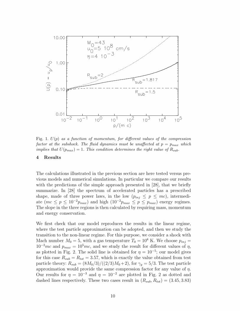
Fig. 1. U(p) as a function of momentum, for different values of the compressionfactor at the subshock. The fluid dynamics must be unaffected at p = pmax whichimplies that U(pmax) = 1. This condition determines the right value of Rsub.

4 Results

The calculations illustrated in the previous section are here tested versus pre-vious models and numerical simulations. In particular we compare our resultswith the predictions of the simple approach presented in [28], that we brieflysummarize. In [28] the spectrum of accelerated particles has a prescribedshape, made of three power laws, in the low (pinj ≤ p ≤ mc), intermedi-ate (mc ≤ p ≤ 10−2pmax) and high (10−2pmax ≤ p ≤ pmax) energy regimes.The slope in the three regions is then calculated by requiring mass, momentumand energy conservation.

We first check that our model reproduces the results in the linear regime,where the test particle approximation can be adopted, and then we study thetransition to the non-linear regime. For this purpose, we consider a shock withMach number M0 = 5, with a gas temperature T0 = 108 K. We choose pinj =10−2mc and pmax = 105mc, and we study the result for different values of η,as plotted in Fig. 2. The solid line is obtained for η = 10−5; our model givesfor this case Rsub = Rtot = 3.57, which is exactly the value obtained from testparticle theory: Rsub = (8M0/3)/((2/3)M0+2), for γg = 5/3. The test particleapproximation would provide the same compression factor for any value of η.Our results for η = 10−3 and η = 10−2 are plotted in Fig. 2 as dotted anddashed lines respectively. These two cases result in (Rsub, Rtot) = (3.45, 3.83)

10

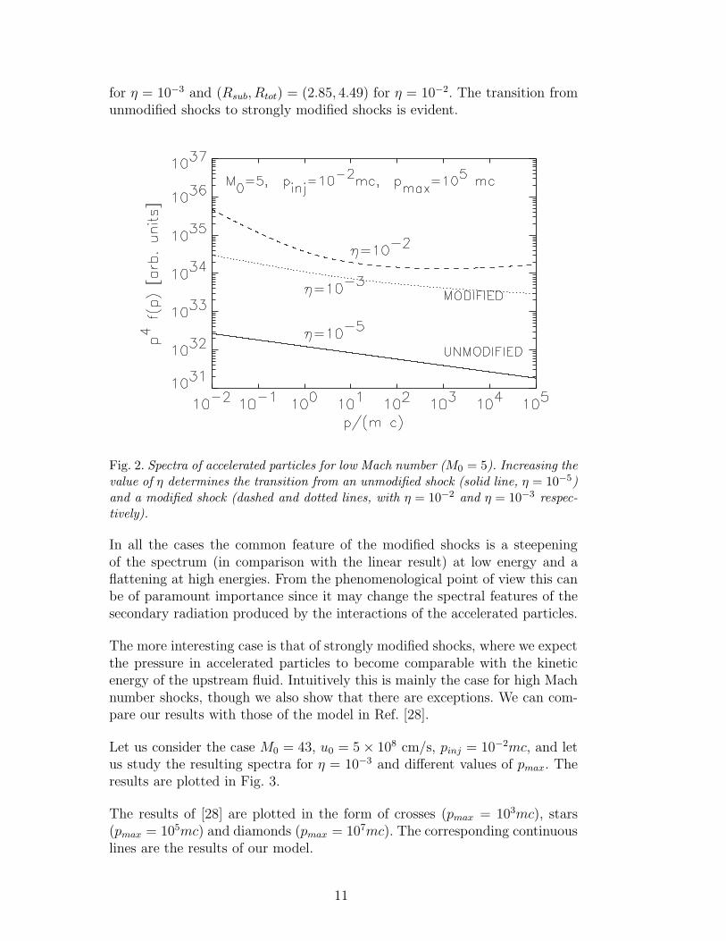
for η = 10−3 and (Rsub, Rtot) = (2.85, 4.49) for η = 10−2. The transition fromunmodified shocks to strongly modified shocks is evident.

Fig. 2. Spectra of accelerated particles for low Mach number (M0 = 5). Increasing thevalue of η determines the transition from an unmodified shock (solid line, η = 10−5)and a modified shock (dashed and dotted lines, with η = 10−2 and η = 10−3 respec-tively).

In all the cases the common feature of the modified shocks is a steepeningof the spectrum (in comparison with the linear result) at low energy and aflattening at high energies. From the phenomenological point of view this canbe of paramount importance since it may change the spectral features of thesecondary radiation produced by the interactions of the accelerated particles.

The more interesting case is that of strongly modified shocks, where we expectthe pressure in accelerated particles to become comparable with the kineticenergy of the upstream fluid. Intuitively this is mainly the case for high Machnumber shocks, though we also show that there are exceptions. We can com-pare our results with those of the model in Ref. [28].

Let us consider the case M0 = 43, u0 = 5 × 108 cm/s, pinj = 10−2mc, and letus study the resulting spectra for η = 10−3 and different values of pmax. Theresults are plotted in Fig. 3.

The results of [28] are plotted in the form of crosses (pmax = 103mc), stars(pmax = 105mc) and diamonds (pmax = 107mc). The corresponding continuouslines are the results of our model.

11

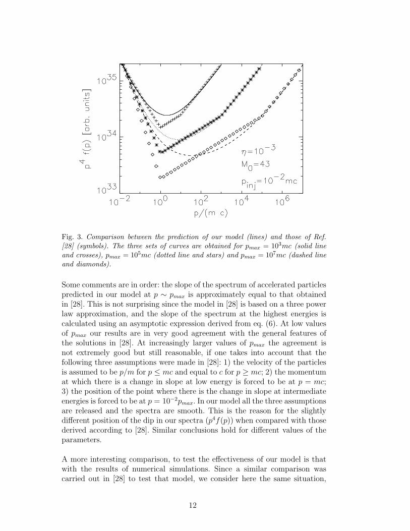
Fig. 3. Comparison between the prediction of our model (lines) and those of Ref.[28] (symbols). The three sets of curves are obtained for pmax = 103mc (solid lineand crosses), pmax = 105mc (dotted line and stars) and pmax = 107mc (dashed lineand diamonds).

Some comments are in order: the slope of the spectrum of accelerated particlespredicted in our model at p ∼ pmax is approximately equal to that obtainedin [28]. This is not surprising since the model in [28] is based on a three powerlaw approximation, and the slope of the spectrum at the highest energies iscalculated using an asymptotic expression derived from eq. (6). At low valuesof pmax our results are in very good agreement with the general features ofthe solutions in [28]. At increasingly larger values of pmax the agreement isnot extremely good but still reasonable, if one takes into account that thefollowing three assumptions were made in [28]: 1) the velocity of the particlesis assumed to be p/m for p ≤ mc and equal to c for p ≥ mc; 2) the momentumat which there is a change in slope at low energy is forced to be at p = mc;3) the position of the point where there is the change in slope at intermediateenergies is forced to be at p = 10−2pmax. In our model all the three assumptionsare released and the spectra are smooth. This is the reason for the slightlydifferent position of the dip in our spectra (p4f(p)) when compared with thosederived according to [28]. Similar conclusions hold for different values of theparameters.

A more interesting comparison, to test the effectiveness of our model is thatwith the results of numerical simulations. Since a similar comparison wascarried out in [28] to test that model, we consider here the same situation,

12

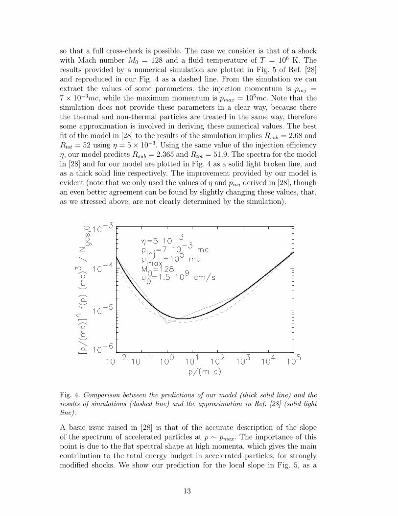
so that a full cross-check is possible. The case we consider is that of a shockwith Mach number M0 = 128 and a fluid temperature of T = 106 K. Theresults provided by a numerical simulation are plotted in Fig. 5 of Ref. [28]and reproduced in our Fig. 4 as a dashed line. From the simulation we canextract the values of some parameters: the injection momentum is pinj =7 × 10−3mc, while the maximum momentum is pmax = 105mc. Note that thesimulation does not provide these parameters in a clear way, because therethe thermal and non-thermal particles are treated in the same way, thereforesome approximation is involved in deriving these numerical values. The bestfit of the model in [28] to the results of the simulation implies Rsub = 2.68 andRtot = 52 using η = 5 × 10−3. Using the same value of the injection efficiencyη, our model predicts Rsub = 2.365 and Rtot = 51.9. The spectra for the modelin [28] and for our model are plotted in Fig. 4 as a solid light broken line, andas a thick solid line respectively. The improvement provided by our model isevident (note that we only used the values of η and pinj derived in [28], thoughan even better agreement can be found by slightly changing these values, that,as we stressed above, are not clearly determined by the simulation).

Fig. 4. Comparison between the predictions of our model (thick solid line) and theresults of simulations (dashed line) and the approximation in Ref. [28] (solid lightline).

A basic issue raised in [28] is that of the accurate description of the slopeof the spectrum of accelerated particles at p ∼ pmax. The importance of thispoint is due to the flat spectral shape at high momenta, which gives the maincontribution to the total energy budget in accelerated particles, for stronglymodified shocks. We show our prediction for the local slope in Fig. 5, as a

13

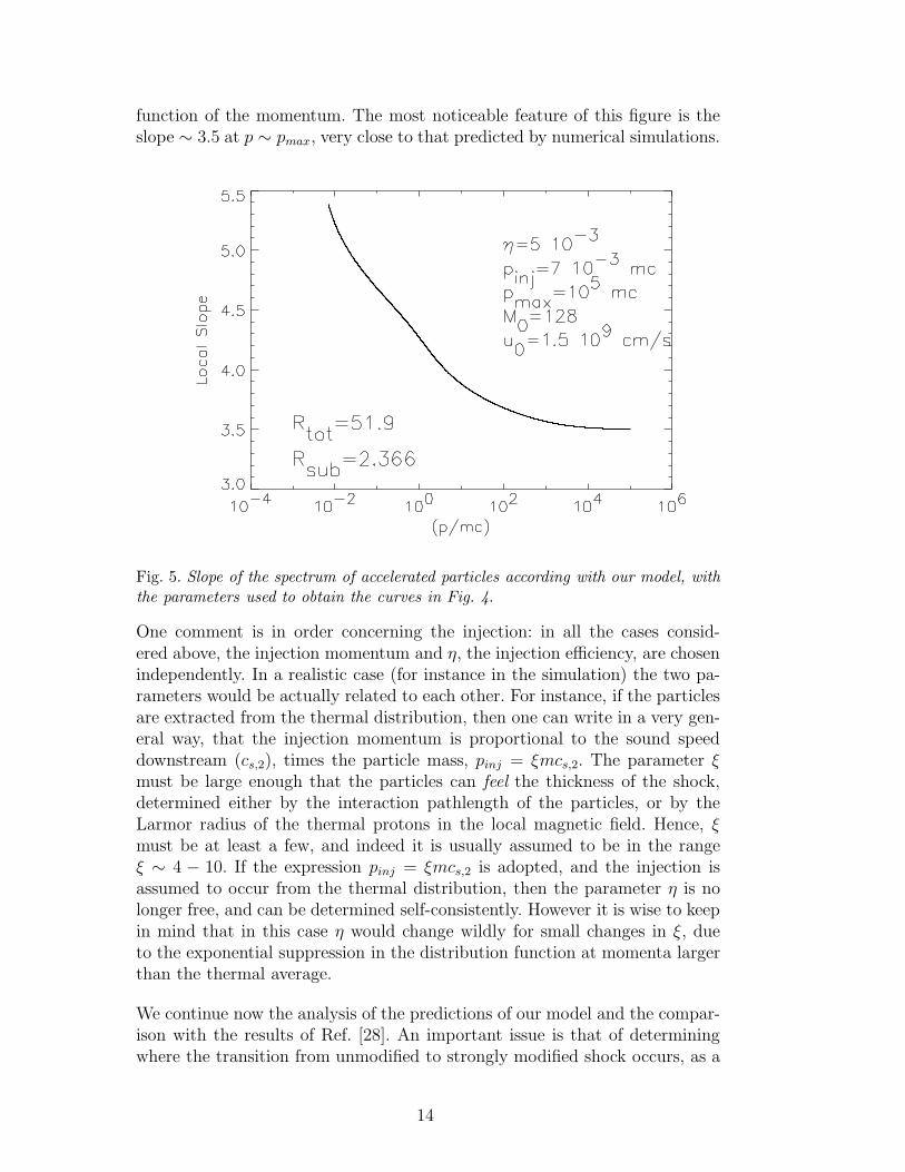
function of the momentum. The most noticeable feature of this figure is theslope ∼ 3.5 at p ∼ pmax, very close to that predicted by numerical simulations.

Fig. 5. Slope of the spectrum of accelerated particles according with our model, withthe parameters used to obtain the curves in Fig. 4.

One comment is in order concerning the injection: in all the cases consid-ered above, the injection momentum and η, the injection efficiency, are chosenindependently. In a realistic case (for instance in the simulation) the two pa-rameters would be actually related to each other. For instance, if the particlesare extracted from the thermal distribution, then one can write in a very gen-eral way, that the injection momentum is proportional to the sound speeddownstream (cs,2), times the particle mass, pinj = ξmcs,2. The parameter ξmust be large enough that the particles can feel the thickness of the shock,determined either by the interaction pathlength of the particles, or by theLarmor radius of the thermal protons in the local magnetic field. Hence, ξmust be at least a few, and indeed it is usually assumed to be in the rangeξ ∼ 4 − 10. If the expression pinj = ξmcs,2 is adopted, and the injection isassumed to occur from the thermal distribution, then the parameter η is nolonger free, and can be determined self-consistently. However it is wise to keepin mind that in this case η would change wildly for small changes in ξ, dueto the exponential suppression in the distribution function at momenta largerthan the thermal average.

We continue now the analysis of the predictions of our model and the compar-ison with the results of Ref. [28]. An important issue is that of determiningwhere the transition from unmodified to strongly modified shock occurs, as a

14

function of the parameters of the calculation.

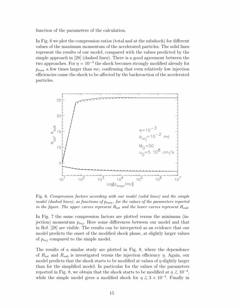
In Fig. 6 we plot the compression ratios (total and at the subshock) for differentvalues of the maximum momentum of the accelerated particles. The solid linesrepresent the results of our model, compared with the values predicted by thesimple approach in [28] (dashed lines). There is a good agreement between thetwo approaches. For η = 10−3 the shock becomes strongly modified already forpmax a few times larger than mc, confirming that even relatively low injectionefficiencies cause the shock to be affected by the backreaction of the acceleratedparticles.

Fig. 6. Compression factors according with our model (solid lines) and the simplemodel (dashed lines), as functions of pmax, for the values of the parameters reportedin the figure. The upper curves represent Rtot and the lower curves represent Rsub.

In Fig. 7 the same compression factors are plotted versus the minimum (in-jection) momentum pinj . Here some differences between our model and thatin Ref. [28] are visible. The results can be interpreted as an evidence that ourmodel predicts the onset of the modified shock phase, at slightly larger valuesof pinj compared to the simple model.

The results of a similar study are plotted in Fig. 8, where the dependenceof Rtot and Rsub is investigated versus the injection efficiency η. Again, ourmodel predicts that the shock starts to be modified at values of η slightly largerthan for the simplified model. In particular for the values of the parametersreported in Fig. 8, we obtain that the shock starts to be modified at η >

∼ 10−4,while the simple model gives a modified shock for η >

∼ 3 × 10−5. Finally in

15

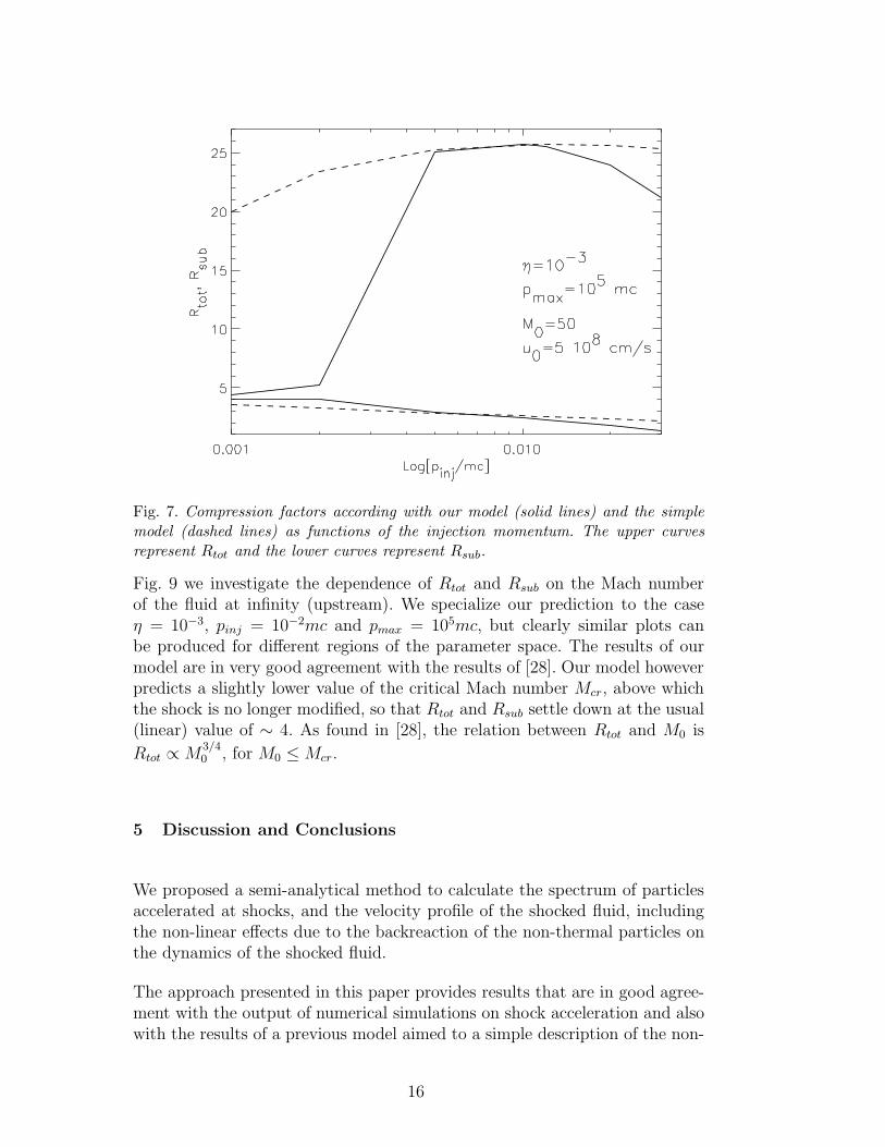
Fig. 7. Compression factors according with our model (solid lines) and the simplemodel (dashed lines) as functions of the injection momentum. The upper curvesrepresent Rtot and the lower curves represent Rsub.

Fig. 9 we investigate the dependence of Rtot and Rsub on the Mach numberof the fluid at infinity (upstream). We specialize our prediction to the caseη = 10−3, pinj = 10−2mc and pmax = 105mc, but clearly similar plots canbe produced for different regions of the parameter space. The results of ourmodel are in very good agreement with the results of [28]. Our model howeverpredicts a slightly lower value of the critical Mach number Mcr, above whichthe shock is no longer modified, so that Rtot and Rsub settle down at the usual(linear) value of ∼ 4. As found in [28], the relation between Rtot and M0 is

Rtot ∝ M3/40 , for M0 ≤ Mcr.

5 Discussion and Conclusions

We proposed a semi-analytical method to calculate the spectrum of particlesaccelerated at shocks, and the velocity profile of the shocked fluid, includingthe non-linear effects due to the backreaction of the non-thermal particles onthe dynamics of the shocked fluid.

The approach presented in this paper provides results that are in good agree-ment with the output of numerical simulations on shock acceleration and alsowith the results of a previous model aimed to a simple description of the non-

16

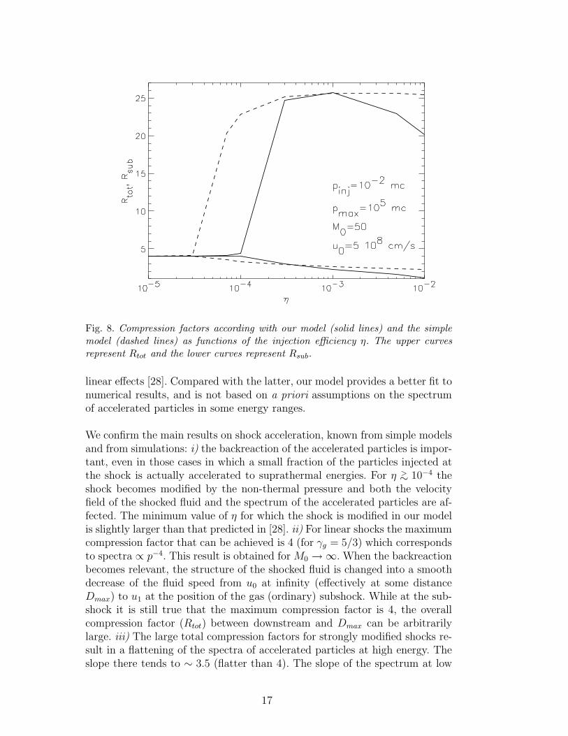
Fig. 8. Compression factors according with our model (solid lines) and the simplemodel (dashed lines) as functions of the injection efficiency η. The upper curvesrepresent Rtot and the lower curves represent Rsub.

linear effects [28]. Compared with the latter, our model provides a better fit tonumerical results, and is not based on a priori assumptions on the spectrumof accelerated particles in some energy ranges.

We confirm the main results on shock acceleration, known from simple modelsand from simulations: i) the backreaction of the accelerated particles is impor-tant, even in those cases in which a small fraction of the particles injected atthe shock is actually accelerated to suprathermal energies. For η >

∼ 10−4 theshock becomes modified by the non-thermal pressure and both the velocityfield of the shocked fluid and the spectrum of the accelerated particles are af-fected. The minimum value of η for which the shock is modified in our modelis slightly larger than that predicted in [28]. ii) For linear shocks the maximumcompression factor that can be achieved is 4 (for γg = 5/3) which correspondsto spectra ∝ p−4. This result is obtained for M0 → ∞. When the backreactionbecomes relevant, the structure of the shocked fluid is changed into a smoothdecrease of the fluid speed from u0 at infinity (effectively at some distanceDmax) to u1 at the position of the gas (ordinary) subshock. While at the sub-shock it is still true that the maximum compression factor is 4, the overallcompression factor (Rtot) between downstream and Dmax can be arbitrarilylarge. iii) The large total compression factors for strongly modified shocks re-sult in a flattening of the spectra of accelerated particles at high energy. Theslope there tends to ∼ 3.5 (flatter than 4). The slope of the spectrum at low

17

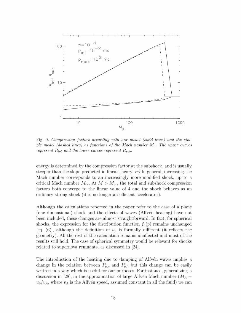
Fig. 9. Compression factors according with our model (solid lines) and the sim-ple model (dashed lines) as functions of the Mach number M0. The upper curvesrepresent Rtot and the lower curves represent Rsub.

energy is determined by the compression factor at the subshock, and is usuallysteeper than the slope predicted in linear theory. iv) In general, increasing theMach number corresponds to an increasingly more modified shock, up to acritical Mach number Mcr. At M > Mcr, the total and subshock compressionfactors both converge to the linear value of 4 and the shock behaves as anordinary strong shock (it is no longer an efficient accelerator).

Although the calculations reported in the paper refer to the case of a plane(one dimensional) shock and the effects of waves (Alfven heating) have notbeen included, these changes are almost straightforward. In fact, for sphericalshocks, the expression for the distribution function f0(p) remains unchanged[eq. (6)], although the definition of up is formally different (it reflects thegeometry). All the rest of the calculation remains unaffected and most of theresults still hold. The case of spherical symmetry would be relevant for shocksrelated to supernova remnants, as discussed in [24].

The introduction of the heating due to damping of Alfven waves implies achange in the relation between Pg,p and Pg,0 but this change can be easilywritten in a way which is useful for our purposes. For instance, generalizing adiscussion in [28], in the approximation of large Alfven Mach number (MA =u0/vA, where vA is the Alfven speed, assumed constant in all the fluid) we can

18

write

Pg,p

Pg,0≃

(

ρp

ρ0

)γg{

1 + (γg − 1)M2

0

MA

[

1 −

(

ρ0

ρp

)γg]}

. (19)

Clearly the effects of Alfven heating can be neglected as long as M20 ≪ MA.

Introducing eq. (19) [instead of eq. (12)] in eq. (10), it is easy to derive anequation similar to eq. (18), that can be solved for U(p). The spectrum ofaccelerated particles is then obtained using the same procedure illustratedabove. The basic effect of the Alfven heating is to reduce the total compressionfactors, and make the spectra at high energy slightly steeper than found in§4.

We conclude by stressing that the non-linear effects discussed here appear tobe relevant even for a small injection efficiency, and their phenomenologicalconsequences can be critically important. For instance, as an application of thesimple model presented in [28], in Ref. [29] the spectra of secondary radio andgamma radiation in supernova remnants were calculated. The differences withrespect to the results obtained by adopting the test particle approximationare impressive.

In this prospective, the semi-analytical model presented here, being of easyuse and having an immediate physical interpretation, provides the suitabletool to estimate the phenomenological consequences of non-linearity in shockacceleration, in the cases where it is unpractical to have access to numericalsimulations.

Acknowledgments This work was supported by the DOE and the NASAgrant NAG 5-7092 at Fermilab.

19

References

[1] T. Tanimori, et al., Astrophys. J. Lett. 497 (1998) L25.

[2] F.A. Aharonian, and A.M. Atoyan, Astron. & Astroph. 351 (1999) 330.

[3] L.O’C. Drury, Rep. Prog. Phys. 46 (1983) 973.

[4] R.D. Blandford, and D. Eichler, Phys. Rep. 154 (1987) 1.

[5] E.G. Berezhko, and G.F. Krimsky, Soviet. Phys.-Uspekhi, 12 (1988) 155.

[6] F.C. Jones, and D.C. Ellison, Space Sci. Rev. 58 (1991) 259.

[7] A.R. Bell, MNRAS 225 (1987) 615.

[8] D.C. Ellison, E. Mobius, and G. Paschmann, Astrophys. J. 352 (1990) 376.

[9] D.C. Ellison, M.G. Baring, and F.C. Jones, Astrophys. J. 453 (1995) 873.

[10] D.C. Ellison, M.G. Baring, and F.C. Jones, Astrophys. J. 473 (1996) 1029.

[11] H. Kang, and T.W. Jones, Astrophys. J. 476 (1997) 875.

[12] L.O’C Drury, and H.J. Volk, Proc. IAU Symp. 94 (1980) 363.

[13] L.O’C Drury, and H.J. Volk, Astrophys. J. 248 (1981) 344.

[14] L.O’C Drury, W.I. Axford, and D. Summers, MNRAS 198 (1982) 833.

[15] W.I. Axford, E. Leer, and J.F. McKenzie, Astron. & Astrophys. 111 (1982) 317.

[16] P. Duffy, L.O’C Drury, and H. Volk, Astron. & Astrophys. 291 (1994) 613.

[17] R. Blandford, Astrophys. J. 238 (1980) 410.

[18] D. Eichler, Astrophys. J. 277 (1984) 429.

[19] D. Ellison, and D. Eichler, Astrophys. J. 286 (1984) 691.

[20] D. Eichler, Astrophys. J. 294 (1985) 40.

[21] D.C. Ellison, and D. Eichler, Phys. Rev. Lett. 55 (1985) 2735.

[22] E.G. Berezhko, V.K. Yelshin, and L.T. Ksenofontov, Astropart. Phys. 2 (1994)215.

[23] E.G. Berezhko, L.T. Ksenofontov, and V.K. Yelshin, Nucl. Phys. B (Proc.Suppl.) 39A (1995) 171.

[24] E.G. Berezhko, Astropart. Phys. 5 (1996) 367.

[25] G. Pelletier, and J. Roland, Astron. & Astroph. 163 (1986) 9.

[26] M.A. Malkov, Astrophys. J. 485 (1997) 638.

[27] M.A. Malkov, P.H. Diamond and H.J. Volk, Astrophys. J. 533 (2000) 171.

[28] E.G. Berezhko, and D.C. Ellison, Astrophys. J. 526 (1999) 385.

[29] D.C. Ellison, E.G. Berezhko, and M.G. Baring, Astrophys. J. 540 (2000) 292.

20