arX

iv:a

stro

-ph/

0503

220v

1 9

Mar

200

5

On particle acceleration around shocks II: a fully general method

for arbitrary shock velocities and scattering media

Pasquale Blasi1 and Mario Vietri2

1 INAF/Osservatorio Astrofisico di Arcetri, Firenze, Italy2 Scuola Normale Superiore, Pisa, Italy

ABSTRACT

The probability that a particle, crossing the shock along a given direction,

be reflected backwards along another direction, was shown to be the key ele-

ment in determining the spectrum of non–thermal particles accelerated via the

Fermi mechanism around a plane–parallel shock in the test–particle limit. Here

an explicit equation for this probability distribution is given, for both the up-

stream and downstream sections. Though analytically intractable, this equation

is solved numerically, allowing the determination of the spectrum in full general-

ity, without limitation to shock speed or scattering properties. A number of cases

is then computed, making contact with previous numerical work, in all regimes:

Newtonian, trans–relativistic, and fully relativistic.

Subject headings: shock waves – cosmic rays

1. Introduction

It is possible to formulate particle acceleration around shocks, in the test particle limit,

in an exact form, for arbitrary shock speeds, and arbitrary anisotropies in the particle dis-

tribution function (Paper I, Vietri 2003). It turns out that the physically relevant boundary

conditions are those at the shock, not those at downstream infinity. These conditions at the

shock fix the particle spectrum which was shown to be (under some simplifying assumptions)

an exact power–law in the particle momentum, independent of the shock speed and of all

assumptions about the scattering properties of the medium.

The exact value of the spectral index depends in a detailed way upon the diffusion prop-

erties of the media involved. It was shown in Paper I that this dependence is encapsulated

in two functions, Pu(µ◦, µ) and Pd(µ◦, µ) respectively, which denote the conditional prob-

abilities that a particle entering the upstream (downstream) medium along a direction µ◦,

– 2 –

will leave it for the downstream (upstream) section along a direction µ1. In paper I (but see

also Freiling, Vietri and Yurko 2003 for some tricky mathematical details), these functions

were built from the eigenfunctions of the angular part of the scattering problem. Though

conceptually satisfactory, this procedure is however computationally tricky, and one may

wonder whether, given the scattering law for the particles, it may be possible to determine

an equation for the scattering probabilities that yields them directly, without having to build

the infinitely many eigenfunctions of the angular equation. It turns out that this is actually

possible, by drawing upon the analogy with scattering atmospheres (Chandrasekhar 1949),

and by using an obvious symmetry property of the problem at hand.

It is the purpose of this paper to present this derivation, and a handful of illustrative

computations, with the major aim of showing the ability of the method to reproduce well–

established results, drawn from the literature. A more detailed analysis of the spectra in

several interesting cases, including the important hyperrelativistic regime, will be presented

elsewhere.

The plan of the paper is as follows: in section 2, we present the derivation of the

equations which determine Pd(µ◦, µ) and Pu(µ◦, µ). In section 3, we show that a diffusive

equation identical to that originally given by Kirk and Schneider (1987) is recovered in the

Fokker–Planck regime (or small–pitch–angle scattering, SPAS) of our scattering equation,

Eq. 2 . In section 4, we describe our full method to compute numerically the spectral slope

and angular distribution function. In section 5 we show that our method reproduces very

well results which have already appeared in the literature, in the newtonian, trans-relativistic

and fully relativistic regimes (the ultra-relativistic regime will be discussed in forthcoming

publication). We conclude in section 6.

2. The equations for Pd and Pu

In paper I, we showed that a suitable, relativistically covariant (though not manifestly

so) equation for the transport of the particle distribution function for arbitrary pitch angle

scattering in the presence of a large-coherence length magnetic field is:

γ(u + µ)∂f

∂z=

∫

(−we(µ′, µ, φ, φ′)f(µ, φ) + we(µ, µ′, φ, φ′)f(µ′, φ′)) dµ′dφ′ + ω

∂f

∂φ. (1)

In this equation, z is the distance from the shock along the shock normal, in the shock frame.

All other quantities are measured in the fluid frame: u is the fluid speed with respect to

1In these expressions, all angles are measured in the fluid frame.

– 3 –

the shock, in units of c, and γ = 1/√

1 − u2 its associated Lorentz factor, f is the DF of

particles with impulse p in the fluid frame (which, by assumption, does not change because

we assumed pitch–angle scattering), and we(µ, µ′, φ, φ′) is the scattering probability that a

particle, originally moving along a direction making an angle with the shock normal such

that its cosine is µ′, and along φ′, be deflected along a new direction µ, φ. The fluid is

assumed to move in the positive z direction, so that its speed is at all places > 0, and the

angles are measured from the direction of motion of the fluid.

The scattering is assumed linear (thus these results apply only in the test particle

approximation), but the scattering angle is nowhere assumed small: we shall derive results

for the diffusive approximation in a later section. This equation is the plane–geometry, fully

relativistic version of an equation originally developed by Gleeson and Axford (1967) for

spherically symmetric, non–relativistic shocks.

Compared with Eq. 7 of Paper I, the injection has been dropped because we are con-

sidering particles at very large energies, much larger than the injection energy; we now also

specialize to the case in which no long-coherence length magnetic field is present. The treat-

ment of the problem in full generality will be presented elsewhere (Morlino, Blasi and Vietri,

in preparation).

Besides dropping the term ω(∂f/∂φ), we remark that the system has now become

symmetric for rotations around the shock normal, so that the DF f will be independent

of the angle φ. Furthermore, the elemental scattering probability we can depend only on

the angle φ − φ′ between the incoming and outgoing direction, we = we(µ, µ′, φ − φ′), even

though it can depend separately upon µ and µ′. In this symmetric case, we can average the

previous equation over either φ or φ′, obtaining

γ(u + µ)∂f

∂z=

∫

(−w(µ′, µ)f(µ) + w(µ, µ′)f(µ′)) dµ′dφ′ , (2)

where

w(µ, µ′) ≡ 1

2π

∫

we(µ, µ′, φ − φ′)dφ , (3)

an equation which will be used later on.

2.1. The downstream case

In order to fix the ideas, we consider the problem of determining Pd, the conditional

probability for the downstream frame; we shall explain later how to adapt these results to the

upstream frame. Take the origin of coordinates to be located at the shock, the downstream

– 4 –

section to be at z > 0, and define u as the modulus of the shock speed with respect to the

fluid. We are using variables in the fluid frame: µ is thus the cosine of the angle between

the particle speed and the shock normal, in the fluid frame. This means that the particles

which can cross from upstream to downstream (i.e., those with a positive component along

the shock normal of the velocity with respect to the shock) are those with

u + µ > 0 , (4)

while those that cross the shock backwards, from the downstream to the upstream section,

have

u + µ < 0 . (5)

Now let f represent a beam of particles, all entering the downstream section along the

same direction, µ◦; we showed in paper I that the particle flux across a surface fixed in the

shock frame, but expressed in downstream coordinates, is given by:

F ≡ F◦γ =

∫

γ(u + µ)fdµ . (6)

We consider now a pencil beam of particles, all moving initially in the direction µ◦. Thus,

at the shock:

f(µ) =F◦

u + µδ(µ − µ◦) u + µ ≥ 0 , (7)

with F◦ an obvious normalization. It was shown in paper I that Eq. 7 provides a suitable

boundary condition for Eq. 2, which then returns the outgoing flux; by definition, this is

precisely the required Pd. We thus have

−(ud + µ)f(µ) = F◦Pd(µ◦, µ) u + µ < 0 . (8)

To begin, let us define the inward (f+ ≡ f(µ)|u+µ>0) and outward (f− ≡ f(µ)|u+µ<0)

parts of the distribution function, and let us consider a surface at a distance z from the

shock, fixed in the shock frame. The flux of particles moving backwards toward the shock,

through this surface, is:

γ(u + µ)f−(µ) = −∫ 1

−u

f+(µ′)γ(u + µ′)Pd(µ′, µ)dµ′ . (9)

The minus sign accounts for the fact that u + µ < 0, while all terms inside the integral are

positive.

Strictly speaking, in the above equation, we should have written Pd(µ′, µ, z) instead of

simply Pd(µ′, µ). In other words, for a general situation, we cannot assume that the condi-

tional probability Pd be independent of its location inside the downstream region. However,

– 5 –

in this case this assumption is fully justified, because the downstream region is semi–infinite:

in other words, it remains identical to itself whenever we add or subtract finite regions, and

its diffusive properties also remain unaltered whenever we add or subtract finite regions. It

follows that the conditional probability Pd from some finite z to downstream infinity must

be exactly identical to that from 0 to downstream infinity. This invariance principle, and

this whole discussion, are identical to those in Chandrasekhar (1949, Chapter 4, Sections

28-29), and provide an exact justification for the equation above.

We now differentiate the above with respect to z:

γ(u + µ)∂f−∂z

= −∫ 1

−u

dµ′γ(u + µ′)∂f+

∂zPd(µ

′, µ) (10)

while Eq. 2 gives us

γ(u + µ)∂f−∂z

= −d(µ)f− +

∫ 1

−u

dµ′w(µ, µ′)f+(µ′) +

∫

−u

−1

dµ′w(µ, µ′)f−(µ′) (11)

γ(u + µ)∂f+

∂z= −d(µ)f+ +

∫ 1

−u

dµ′w(µ, µ′)f+(µ′) +

∫

−u

−1

dµ′w(µ, µ′)f−(µ′) , (12)

where we used the shorthand

d(µ) ≡∫

w(µ′, µ)dµ′ . (13)

We now evaluate Eq. 11 at z = 0, using Eqs. 7 and 8, to obtain

γ(u + µ)∂f−∂z

|◦ =F◦d(µ)

γ(u + µ)Pd(µ◦, µ) +

F◦w(µ, µ◦)

γ(u + µ◦)−

∫

−u

−1

dµ′w(µ, µ′)F◦Pd(µ◦, µ

′)

γ(u + µ′). (14)

We can now proceed analogously for Eq. 12: we again evaluate it at z = 0, and use Eqs. 7

and 8, to obtain:

γ(u + µ)∂f+

∂z|◦ = − F◦d(µ)

γ(u + µ)δ(µ − µ◦) +

F◦w(µ, µ◦)

γ(u + µ◦)−

∫

−u

−1

dµ′w(µ, µ′)F◦Pd(µ◦, µ

′)

γ(u + µ′). (15)

As our last step, we plug Eqs. 14 and 15 into Eq. 10 to obtain:

Pd(µ◦, µ)

(

d(µ◦)

u + µ◦

− d(µ)

u + µ

)

=w(µ, µ◦)

u + µ◦

+

∫ 1

−u

dµ′Pd(µ

′, µ)w(µ′, µ◦)

u + µ◦

−∫

−u

−1

dµ′Pd(µ◦, µ

′)w(µ, µ′)

u + µ′−

∫ 1

−u

dµ′Pd(µ′, µ)

∫

−u

−1

dµ′′w(µ′, µ′′)Pd(µ◦, µ

′′)

u + µ′′(16)

which is the sought–after result: an equation relating Pd only to the diffusion probability w.

– 6 –

2.2. The upstream case

A completely analogous derivation holds in this case. The pencil beam is now entering

the upstream section, so that, at the shock, we have:

f(µ) = − F◦

u + µδ(µ − µ◦) u + µ ≤ 0 (17)

and we have the obvious definition, from paper I:

f(µ) =F◦

u + µPu(µ◦, µ) u + µ > 0 . (18)

At a distance z from the shock the flux of particles moving toward the shock is

γ(u + µ)∂f+

∂z= −

∫

−u

−1

dµ′γ(u + µ′)Pu(µ′, µ)

∂f−∂z

(19)

where the same argument about the use of Pu(µ′, µ) instead of Pu(µ

′, µ, z) applies as above.

We may evaluate the above equation at z = 0 using Eqs. 11 and 12 (which still hold), and

Eqs. 17 and 18, and plug the result into Eq. 19, to obtain

Pu(µ◦, µ)

(

d(µ◦)

u + µ◦

− d(µ)

u + µ

)

=w(µ, µ◦)

u + µ◦

−∫ 1

−u

dµ′w(µ, µ′)Pu(µ◦, µ

′)

u + µ′+

∫

−u

−1

dµ′w(µ′, µ◦)Pu(µ

′, µ)

u + µ◦

−∫

−u

−1

dµ′Pu(µ′, µ)

∫ 1

−u

dµ′′w(µ′, µ′′)Pu(µ◦, µ

′′)

u + µ′′(20)

which is our other final result.

3. The small–pitch–angle limit

In this section, we wish to derive the small pitch–angle scattering (SPAS) limit of our

scattering equation, which holds for arbitrary deflection angles, not just small ones. Before

proceeding with the derivation of the Fokker–Planck equation, we need to establish a very

useful result. The function w is not completely arbitrary, but is subject to the following

requirement. We expect that, when the distribution function (DF) is isotropic (i.e., when

f(µ) = const.), there will be no further evolution: in other words, we expect in this case

the RHS of the above equation to vanish. For this to occur, we shall not take the obvious

condition∫ +1

−1

w(µ, µ′)dµ′ =

∫ +1

−1

w(µ′, µ)dµ′ (21)

– 7 –

but its stronger version,

w(µ, µ′) = w(µ′, µ) . (22)

The above equation is a statement of detailed balance, which we may assume to hold because

these scattering processes are exactly those which lead to isotropization of the DF, if thermal

equilibrium were to hold. In our case we have neglected (for excellent, well–known reasons)

the exchange of energy of the particles with the background fluid, so we cannot expect true

thermal equilibrium to hold, but since we have included all major scattering processes, we

expect equilibrium (i.e., detailed balance except for energy equipartition) to hold at least in

so far as the angular part is concerned. It is probably worthwhile to remark that a similar

assumption on w is made by Chandrasekhar (1949, Ch. IV, Section 31, Eq. 29-1).

We now rewrite Eq. 2 by means of a new scattering probability, W (µ′; α), to be defined

as follows:

W (µ′; α)dα ≡ w(µ′ + α, µ′)d(µ′ + α) . (23)

W is simply the probability that a particle is deflected from its initial direction along µ′, to

a new direction µ′ + α. By means of this new quantity Eq. 2 can be recast as:

γ(u + µ)∂f

∂z=

∫ +1

−1

dα (W (µ − α; α)f(µ− α) − W (µ;−α)f(µ)) (24)

while the detailed balance equation becomes:

W (µ − α; α) = W (µ;−α) . (25)

The scattering equation in the form 24 is exactly identical to that given by Landau

and Lifshtiz (1984, Section 21, Eq. 21.1), so that their derivation of the Fokker–Planck

immediately applies. Please note however that our sign convention differs from theirs: what

we call α is for them −q. Following step by step their derivation we find that

γ(u + µ)∂f

∂z≈ ∂

∂µ

(

Af + B∂f

∂µ

)

, (26)

with the definitions

A ≡ −∫ +∞

−∞

dα αW (µ; α) +∂B

∂µ(27)

B ≡ 1

2

∫ +∞

−∞

dα α2W (µ; α) . (28)

In the two integrals above, we have taken the integration range to extend from −∞ to +∞,

because we have assumed the validity of the SPAS regime, in which case W (µ; α) has one

very strong, narrow peak around α = 0:

– 8 –

We show now that, as a consequence of detailed balance, A = 0. We first notice that

∂

∂µW (µ; α) =

∂

∂µW (µ′; µ − µ′) (29)

where µ′ = µ + α, because of detailed balance, so that

∂

∂µW (µ; α) =

∂

∂αW (µ′; α) . (30)

We use the above into

∂B

∂µ=

1

2

∫ +∞

−∞

dα α2 ∂

∂µW (µ; α) =

1

2

∫ +∞

−∞

dα α2 ∂

∂αW (µ′; α) (31)

which can now be integrated by parts to yield

∂B

∂µ= −

∫ +∞

−∞

dα αW (µ′; α) . (32)

We now use again detailed balance, and the variable change x ≡ −α in the definite integral

above, to obtain∂B

∂µ=

∫ +∞

−∞

dα αW (µ; α), (33)

which, when inserted into Eq. 27, yields A = 0. We thus obtain, for the scattering equation

in the SPAS, or Fokker–Planck, limit:

γ(u + µ)∂f

∂z=

∂

∂µ

(

B∂f

∂µ

)

, (34)

with B given by Eq. 28. The use of detailed balance implies that the scattering integral

reduces, in the SPAS limit, to the divergence of a vector proportional to the gradient of the

DF, exactly like in the classical heat conduction problem.

As a simple test of this treatment, we now re-derive a well–known result, i.e., that, in

the isotropic limit,

B = K(1 − µ2) (35)

with K a constant. The isotropic limit means that the scattering coefficient probability W

can only depend on the angle θ − θ′ between the directions of motion. We shall take thus

W (µ; α) = Nf(ξ) (36)

where

ξ ≡ sin(θ − θ′)

σ, (37)

– 9 –

with σ a parameter which we take σ ≪ 1, in order to enforce the SPAS regime. Also, we

assume that f(x) is an even function of x, with a single minimum around x = 0 (again,

SPAS regime); we also assume, for the moment, that W is normalized to unity:

∫ +∞

−∞

dαNf(α) = 1 , (38)

and will come back to this assumption in a moment.

We now compute B from Eq. 28. Since we shall be taking the limit σ → 0, only the

argument sin(θ − θ′) ≈ σ ≪ 1 will contribute to the integral, so that, defining ǫ ≡ θ − θ′,

we find

ξ ≈ ǫ

σ(39)

α ≡ µ′ − µ = cos θ′ − cos θ = cos(θ + ǫ) − cos θ ≈ − sin θǫ (40)

so that the normalization condition, Eq. 38 requires

N =

(

sin θσ

∫ +∞

−∞

f(ǫ

σ)d

ǫ

σ

)−1

. (41)

B then becomes

B =1

2

∫ +∞

−∞

dα α2W (µ; α) ≈ 1

2Nσ3 sin3 θ

∫ +∞

−∞

f(ξ)ξ2dξ =

sin2 θσ2

∫ +∞

−∞ξ2f(ξ)dξ

∫ +∞

−∞f(x)dx

(42)

which is clearly identical to Eq. 35. If we now assume W to have arbitrary normalization

(because it represents the probability of scattering per unit time), we see that the above

derivation is changed only through an inessential multiplicative constant. This completes

our derivation.

3.1. Scattering probability

Later on, we shall compare numerical results based upon our new approach with those

which previous authors have obtained in the fully isotropic, small pitch angle scattering limit.

In order to do this, we have to determine a suitable form for w in this case. It is clear that

any function very strongly peaked around the forward direction simulates the SPAS regime,

like, for instance,

w ∝ e−(µ−µ′)2/2σ2

, σ ≪ 1 . (43)

– 10 –

However, not all such peaked functions reproduce the isotropic case, which is defined as that

in which the elemental scattering probability we is independent of anything except for the

deflection angle:

we(µ, µ′, φ, φ′) = w(cos Θ) (44)

with Θ given by

cos Θ ≡ µµ′ +√

1 − µ2√

1 − µ′2 cos(φ − φ′) . (45)

We have seen above that the transport equation in the SPAS regime does not depend upon

the exact form of the scattering function we, so that we are free to choose any analytically

tractable one. We choose:

we(cos Θ) =1

σe−

1−cos Θ

σ , σ ≪ 1 , (46)

which is obviously suitably normalized to unity when the integral is made over all scattering

angles. Using Eq. 3 we find now

w =1

2π

∫ 2π

0

wed(φ − φ′) =1

σe−

1−µµ′

σ I0(

√

1 − µ2√

1 − µ′2

σ) (47)

where I0(x) is Bessel’s modified function of order 0, and use has been made of the formula

(Gradshteyn and Ryzhik, 1994, 3.339):

∫ π

0

exp(z cos x)dx = πI0(z) . (48)

In the following we shall use Eq. 47 when computing spectra, taking σ ≪ 1 for the isotropic

SPAS limit and σ ≫ 1 for the isotropic large angle scattering regime.

4. Calculation of the spectrum and angular distribution function

In this section we outline the procedure to follow in order to calculate the spectral slope

and the angular distribution function of the accelerated particles, for an arbitrary choice of

the shock velocity and of the scattering properties of the fluid.

For the purpose of making contact with previous literature on the subject, we carry

out our calculations with a scattering function w(µ, µ′) as given in Eq. 47, choosing a small

value of the parameter σ for the case of small pitch angle scattering, and a large value of

σ to reproduce the regime of large angle scattering. Eq. 47 ensures that the scattering

remains isotropic in both regimes. However, we wish to stress that we elected to use an

isotropic scattering in order to make contact with all other authors (so far), who have only

– 11 –

used isotropic scattering, even though this is by no means required by our method, which

can effectively deal with anisotropic scattering.

It is worth stressing that our method does not require any intrinsic approximations or

assumptions on the type of scattering; the only approximations are due to round-off in the

numerical solution of the integral equations for Pd and Pu.

The procedure for the calculation of the slope of the spectrum of accelerated particles

is as follows: for a given Lorentz factor of the shock (γsh), the velocity of the upstream

fluid u = βsh is calculated. We then determine the velocity of the downstream fluid ud from

the conventional jump conditions at the shock, after assuming some equation of state for

the post–shock fluid. Given u, ud and a scattering function w, we can solve the integral

equations for Pu and Pd iteratively. We recall here that these are functions of an entrance

and an exit angle, and the convergence of the method can be numerically time consuming, in

particular for small values of σ. Aside from this numerical issue, one should also remember

that our equations for Pu and Pd are analogous to the H-equation of Chandrasekhar (which

is however in one dimension only) which is known to admit multiple solutions. It has been

shown however (Kelley 1982) that iterative methods always converge to the only physically

meaningful solution, although no information is provided on how fast the convergence is

achieved.

An important point to keep in mind is that the probability of return from the upstream

section is strongly constrained through the condition that all particles must return to the

shock, being advected with the fluid. It follows that

∫ 1

−u

dµ′Pu(µ0, µ′) = 1

for any value of the entrance angle µ0. It should be stressed however that this integral con-

straint is not imposed by hand. In other words, though dictated by physical considerations,

it is automatically implemented by the integral equation for Pu (Eq. 20): it thus provides

an important numerical check of our computing accuracy.

The slow convergence of the iterative solution of Eq. 16 has been partly corrected by use

of the following ruse. The conditional probability Pd obeys the following integral constraint.

From Eq. 2 we see that at downstream infinity the condition ∂f/∂z = 0 implies that the

only physically acceptable solution for the distribution function is f(µ) = constant = K. At

downstream infinity we can therefore write

f−(µ)(u+µ) = K(u+µ) = −∫ 1

−ud

dµ′f+(µ′)(u+µ′)Pd(µ′, µ) = −

∫ 1

−ud

dµ′K(u+µ′)Pd(µ′, µ),

(49)

– 12 –

which implies the condition

∫ 1

−ud

dµ′(ud + µ′)Pd(µ′, µ) = −(ud + µ) (50)

for any value of the exit angle µ. Since the function Pd depends only on the scattering

properties of the fluid, which are assumed to be independent of z, Eq. 50 also applies to any

z, including z = 0 which is the position of the shock.

This condition is of course automatically satisfied at the end of our calculations, while

it is only approximately satisfied during the iterative solution of Eq. 16. We have found out

that, by correcting the normalization of Pd so that it obeys the previous integral constraint

to hold at the end of every iteration, the convergence is much accelerated, above all in the

SPAS regime. We are unable to explain why this occurs, but shortening of the computation

times by a factor of 3, or more, have thus been achieved.

Once the two functions Pu and Pd have been calculated, the slope of the spectrum, as

discussed in paper I, is given by the solution of the equation:

(ud + µ)g(µ) =

∫ 1

−ud

dξQT (ξ, µ)(ud + ξ)g(ξ), (51)

where

QT (ξ, µ) =

∫

−ud

−1

dνPu(ν, µ)Pd(ξ, ν)

(

1 − urelµ

1 − urelν

)3−s

. (52)

Here urel = u−ud

1−uudis the relative velocity between the upstream and downstream fluids

and g(µ) is the angular part of the distribution function of the accelerated particles, which

contains all the information about the anisotropy. A point to notice concerns the function

Pu in Eq. (52): all variables and functions here are evaluated in the downstream frame,

while the Pu calculated though Eq. (20) is in the frame comoving with the (upstream) fluid.

The Pu that need to be used in Eq. (52) is therefore

Pu(ν, µ) = Pu(ν̃, µ̃)dµ̃

dµ= Pu(ν̃, µ̃)

[

1 − u2rel

(1 − urelµ)2

]

.

The solution for the slope s of the spectrum is found by solving Eq. 51. In general, this

equation has no solution but for one value2 of s. Finding this value provides not only the

slope of the spectrum but also the angular distribution function g(µ).

2The fact that the solution is unique could not be demonstrated rigorously, but in our calculations we

never found cases of multiple solutions.

– 13 –

5. Comparison with previous results

In this section we apply the method detailed above to several cases that have already

been discussed in the literature, in order to show that the approach can be successfully

applied to a variety of cases. More specifically, we consider the following test situations:

• Since our method is not based on the assumption of small pitch angle scattering, we

can demonstrate that the slope of the spectrum of particles accelerated at Newtonian

shocks is independent of the scattering function w(µ, µ′), although the functions Pd

and Pu in general do depend on the choice of w.

• To our knowledge, the only calculation of the functions Pd and Pu which applies to

shocks of arbitrary velocity for the case of large angle scattering is that of Kato &

Takahara (2001). We compare our results for Pd and Pu with those presented in

that paper for a scattering function which reproduces the physical case of large angle

scattering.

• The slope of the spectrum of accelerated particles in the relativistic regime for the case

of large angle scattering was compared with the results of Monte Carlo calculations

carried out by Ellison, Jones and Reynolds (1990).

• The case of small pitch angle scattering was assumed in most previous calculations.

We test our approach in this regime in two ways: 1) by showing that the slope of the

spectrum of accelerated particles in the SPAS approximation, as computed through our

method for several values of the shock Lorentz factor, compares well with the results

presented in (Kirk et al., 2000); 2) by comparing our angular distribution function with

that obtained by Kirk & Schneider (1987) for a given relativistic shock velocity.

5.1. The Newtonian case

The theoretical approach presented here allows us to determine the spectrum and the

anisotropy in the particle distribution for arbitrary shock velocity and arbitrary scattering

properties of the fluid. In this section we show that we can reproduce the results expected

in the non-relativistic limit. We calculated the spectral slope and the angular part of the

distribution function for several values of the shock velocity and shock compression factor

r. We also calculated the return probability from the downstream and upstream sections.

The expected return probability in the Newtonian limit is P dret = 1 − 4ud, very accurately

reproduced by our calculation, for instance for ud = 10−2 (P dret = 0.96) and for ud = 2×10−2

– 14 –

Fig. 1.— Probability functions Pd(µ0, µ) and Pu(µ0, µ) for u = 0.03 and ud = 0.01 for

σ = 0.01, at fixed values of µ0 (as indicated).

(P dret = 0.92). In all cases that we considered, the condition

∫ 1

−u

dµ′Pu(µ0, µ′) = 1

is confirmed for any value of µ0 within a part in 104. As a matter of fact, we checked that

the above equality is satisfied in all cases we studied, relativistic or otherwise.

The slope of the spectrum of accelerated particles for u = 3 × 10−2 and ud = 10−2

(compression factor 3) as calculated with our approach is 4.5, in agreement with the theo-

retical prediction (Bell 1978). We obtain the same slope in both cases of small pitch angle

scattering with σ = 0.01 and large angle scattering, that we simulate by choosing σ = 100

(but any large value gives the same result). The fact that in the newtonian limit the slope of

the spectrum does not depend on the scattering properties of the fluid is also in agreement

with the theoretical prediction of Bell (1978). It is worth stressing that this universality in

the spectrum of the accelerated particles does not reflect in the universality of the return

probabilities Pd and Pu. In Fig. 1 we plot Pd(µ0, µ) and Pu(µ0, µ) as functions of µ for the

values of µ0 indicated in the figure and assuming u = 0.03, ud = 0.01 and σ = 0.01. The

same functions are plotted in Fig. 2 for the case of large angle scattering (σ = 100).

5.2. The probability functions Pd and Pu for the relativistic regime and large

angle scattering

As stressed above, our method is based on the introduction of the two probability

distributions Pd and Pu, that can be calculated by solving two integral equations, Eqs. (16)

– 15 –

Fig. 2.— Probability functions Pd(µ0, µ) and Pu(µ0, µ) for u = 0.03 and ud = 0.01 for

σ = 100 (large angle scattering), at fixed values of µ0 (as indicated).

Fig. 3.— Return probabilities Pd(µ0, µ) (left) and Pu(µ0, µ) (right) that a particle entering

the downstream (upstream) region with an angle having cosine µ0, exits it with an angle

having cosine µ, for the values of µ0 as indicated.

and (20). The only other approach that we are aware of, that introduces these two functions

is that presented by Kato & Takahara (2001), based on the theory of random walk. We

apply our calculations to reproduce Fig. 6 of their paper, obtained for a fluid speed u = 0.5

both upstream and downstream and in the regime of large angle scattering.

We plot our results in Fig. 3 for the functions Pd (left panel) and Pu (right panel). We

carry out our calculations for exactly the same values of µ0 as indicated in Fig. 6 of Kato

& Takahara (2001) and reported in our Fig. 3 as well. It is worths stressing that for the

downstream section of the fluid ud + µ0 > 0 and ud + µ < 0, while for the upstream section

these relations have opposite signs.

– 16 –

There is perfect agreement between our results and those of Fig. 6 of Kato and Takahara

(2001), which is further evidence that our method is perfectly able to reproduce previous

results, despite the absolute absence of any physical approximation.

5.3. The spectrum for the case of large angle scattering

The spectrum of the accelerated particles for the case of pure large angle scattering

was calculated by Kato & Takahara (2001) and there compared with the previous Monte

Carlo result of Ellison et al. (1990). The case of mixed small and large angle scattering was

investigated by Kirk & Schneider (1988).

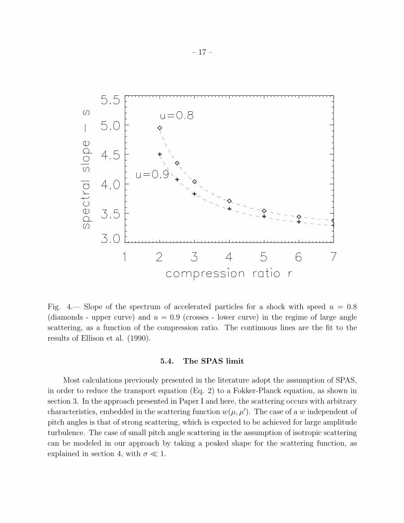
We apply our method to determine the spectrum of accelerated particles for pure large

angle scattering and compare our results with those previously obtained by Kato & Taka-

hara (2001) and by Ellison et al. (1990), which were slightly discrepant for relativistic shock

speeds. The spectral slopes calculated according with the procedure defined in the previous

section are plotted in Fig. 4 for shock speeds u = 0.8 and u = 0.9 as functions of the com-

pression factor r at the shock. The crosses and diamonds are the results of our calculations,

while the continuous curves represent the interpolation provided by Ellison et al. (1990) to

their Monte Carlo results.

It is remarkable that, while the probability distributions Pd and Pu computed by us and

by Kato and Takahara (2001) agree perfectly, our slopes differ from theirs. We speculate

that this is due to the different method of computation. Kato and Takahara (2001) use

Peacock’s recipe:

P < G >s−3= 1 (53)

where < G > is the average energy fractional gain when a whole cycle upstream → down-

stream → upstream is performed. However, in paper I, we showed that the correct formula

is

P < Gs−3 >= 1 (54)

which obviously differs from the previous one. The fact that our computations, on the one

hand, match the functions Pd and Pu of Kato and Takahara, but on the other one reproduce

so perfectly the slopes of Ellison, Jones and Reynolds (1990) (which use neither our approach

nor Peacock’s) supports our claim that our formula is the correct one.

– 17 –

Fig. 4.— Slope of the spectrum of accelerated particles for a shock with speed u = 0.8

(diamonds - upper curve) and u = 0.9 (crosses - lower curve) in the regime of large angle

scattering, as a function of the compression ratio. The continuous lines are the fit to the

results of Ellison et al. (1990).

5.4. The SPAS limit

Most calculations previously presented in the literature adopt the assumption of SPAS,

in order to reduce the transport equation (Eq. 2) to a Fokker-Planck equation, as shown in

section 3. In the approach presented in Paper I and here, the scattering occurs with arbitrary

characteristics, embedded in the scattering function w(µ, µ′). The case of a w independent of

pitch angles is that of strong scattering, which is expected to be achieved for large amplitude

turbulence. The case of small pitch angle scattering in the assumption of isotropic scattering

can be modeled in our approach by taking a peaked shape for the scattering function, as

explained in section 4, with σ ≪ 1.

– 18 –

We expect that in the limit of SPAS the result should not depend upon the detailed

form of the scattering function, provided this is strongly peaked (see Section 3).

For a given Lorentz factor of the shock (γsh), the velocity of the upstream fluid u = βsh

is calculated. For the purpose of comparing our results with those of Kirk et al. (2000),

we adopt a Synge (1957) equation of state for the downstream fluid and assume that the

magnetic field is not dynamically important. These are the same assumptions as in (Kirk et

al. 2000).

We can therefore calculate the velocity of the downstream fluid ud from the conservation

of mass, momentum and energy at the shock surface. The values of u and ud are given in

Table 1. Given these velocities and a width σ for the scattering function, we can solve the

integral equations for Pu and Pd iteratively.

γshβsh u ud slope

0.04 0.04 0.01 4.00

0.2 0.196 0.049 3.99

0.4 0.371 0.094 3.99

0.6 0.51 0.132 3.98

1.0 0.707 1.191 4.00

2.0 0.894 0.263 4.07

4.0 0.97 0.305 4.12

5.0 0.98 0.311 4.13

Following the procedure outlined in section 4, we determine the slope of the power law

spectrum and the angular part g(µ) of the distribution function.

The slopes predicted by our calculations for different values of the shock velocity are

shown in Table 1 for σ = 0.01 and agree well with those of Kirk et al. (2000). In Fig. 5 we

also plot the distribution functions obtained for all the cases reported in Table 1 (the upper

panel refers to the first four lines in Table 1, while the lower panel refers to the relativistic

regime, namely the last four lines in Table 1).

This figure shows the expected phenomenon of increasing anisotropy in the distribution

funtion when the shock speed increases: for non-relativistic speeds the distribution function is

almost perfectly independent of the pitch angle µ, but it becomes more and more anisotropic

in the trans-relativistic regime and in the fully relativistic regime.

A necessary condition for the SPAS regime to be at work is that σ ≪ 1/4γ2sh. This

implies that the SPAS assumption requires increasingly lower values of σ when the Lorentz

– 19 –

Fig. 5.— Upper panel: DF for γshβsh = 0.04 (solid line), γshβsh = 0.2 (dotted line),

γshβsh = 0.4 (dashed line) and γshβsh = 0.6 (dash-dotted line). Lower panel: DF for

γshβsh = 1 (dash-dotted line), γshβsh = 2 (dashed line), γshβsh = 4 (dotted line) and

γshβsh = 5 (solid line).

factor of the shock increases. For σ = 0.01, the maximum Lorentz factor for which we can

assume to be in the SPAS regime is γsh ∼ 5, and in fact we can already see that the slopes

that we obtain for γshβsh = 5 are slightly smaller than those of Kirk et al. (2000). This

effect will be discussed in detail in a forthcoming paper.

It is worth reminding that the SPAS approximation is in fact expected to be broken in

Nature in the relativistic regime: this is due to the fact that a FP equation describes well

the scattering only when particles scatter many times within a given angle. In the upstream

section, particles are caught up by the shock as soon as their deflection angle with respect to

the normal to the shock is larger than 1/γsh. For relativistic shocks, this quantity becomes

small and eventually comparable with the average deflection angle per unit length, and a

– 20 –

description by means of a Fokker–Planck equation becomes inadequate, as remarked many

times in the literature (Kirk et al., 2000). We stress here that the fact that our method is

not based upon the SPAS approximation, but on the more general Eq. 2, makes it more

widely applicable then previous approaches. Its potential for a more correct investigation of

the large γ limit will have to be investigated elsewhere.

An additional evidence of how important these effects can be for the determination of

the correct distribution function of the accelerated particles is illustrated below. We calculate

here the spectrum and the function g(µ) for u = 0.9 and for the relativistic equation of state

for the downstream gas (uud = 1/3), as adopted by Kirk & Schneider (1987). We carry

out our calculations for σ = 0.05, 0.03, 0.01 and 0.005. The slopes in the four cases are

very close to each other (s = 4.68, 4.69, 4.71, 4.71) but the angular distribution functions

(normalized to be unity at the peak) appear slightly different. It is remarkable however that

when the SPAS regime is approached, the DF converges exactly to that found by Kirk &

Schneider (1987), as illustrated in Fig. 6, where we plotted g(µ) for the four cases mentioned

above: compare our results with Kirk and Schneider’s Fig. 6. The slope that we obtain is

also in perfect agreement with Kirk & Schneider (1987).

6. Conclusions

In Paper I, a new analytic approach to the calculation of the spectrum of particles accel-

erated at a shock surface moving with arbitrary velocity was proposed. In the present paper

we described the procedure to calculate the probability functions Pd(µ0, µ) and Pu(µ0, µ) in-

troduced in Paper I. These two functions allow us to calculate the spectrum and the angular

distribution function of the accelerated particles at the shock, for arbitrary shock velocity

and for arbitrary scattering function w.

We tested the approach in several situations, in order to show that all results previously

appeared in the literature could be successfully reproduced. In particular the following tests

have been performed:

• we confirmed the universality of the slope of the power law spectrum of accelerated

particles in the case of Newtonian shocks. More specifically we proved that such slope

is roughly independent of the scattering properties of the medium, as described by the

scattering function w. It should be stressed that such universality does not extend

to the probability functions Pd and Pu, which are instead strongly dependent upon

the scattering properties. Despite the difference between these probability functions,

their combination results in an angular part of the distribution function of accelerated

– 21 –

Fig. 6.— The angular distribution function g(µ) for u = 0.9 and for the relativistic equation

of state for the downstream gas uud = 1/3. The solid, dotted, dashed and dot-dashed lines

refer respectively to σ = 0.005, 0.01, 0.03 and 0.05.

particles which is approximately flat, as expected in the Newtonian limit (isotropy).

• We checked the correctness of the probability functions Pd and Pu in the case of large

angle scattering by comparing our results with those of Kato & Takahara (2001). We

emphasize that these two functions contain all the physical information about the

spectrum and angular distribution of the accelerated particles.

• We reproduce exceptionally well the results of the Monte Carlo experiments of Ellison

et al. (1990) on the slope of the spectrum of accelerated particles as a function of the

shock compression ratio for different shock speeds, in the large angle scattering regime,

but not Kato and Takahara’s (2001) results. We ascribed this discrepancy to Kato and

Takahara’s use of the (incorrect) Peacock’s formula for the spectral slope.

– 22 –

• We carried out calculations for the case of a scattering function very peaked as a

function of the difference between the cosines of the entrance and exit angles. We

adopted a w in the form given by our Eq. 47. The case of small σ is expected to

describe the limit of isotropic small pitch angle scattering, which is adopted in most

literature on shock acceleration. We showed that in this limit the transport equation

(Eq. 2) reduces to a Fokker-Planck equation, identical to that used for instance by

Kirk & Schneider (1987) and Kirk et al. (2000). We carried out computations for

σ = 0.05 − 0.005, and we compared our predicted spectral slopes with those of Kirk

et al. (2000) for different values of the shock velocity. Our results are illustrated in

Table 1 and show that our method reproduces faily well the SPAS results. Moreover,

our approach shows the expected deviations from the SPAS regime when the condition

σ ≪ 1/(4γ2sh) is violated.

• We have also compared our distribution function at the shock with that published by

Kirk and Schneider (1987), obtaining very good agreement, and an identical slope. We

also show that the distribution function becomes increasingly different when the strict

SPAS regime is broken (Fig. 6).

On the basis of the tests carried out to check our approach, we can claim that this method

of calculation of the spectrum and angular distribution function of particles accelerated

at shocks of arbitrary velocity and arbitrary (but spatially homogeneous) scattering

properties of the fluid is fully successful in reproducing old results, and it can now be applied

to situations which go beyond the well studied case of small pitch angle scattering. In a

forthcoming paper we will describe the potential of this new approach to describe particle

acceleration at ultra-relativistic shocks, including the effect of a possible large scale magnetic

field.

A sincere thanks is due to the referee, whose selfless work has considerably improved an

early version of this work.

REFERENCES

Bell, A.R., 1978, MNRAS, 182, 147; Bell, A.R., 1978, MNRAS, 182, 443.

Chandrasekhar, S., 1949, Radiative Transfer, Dover, New York.

Ellison, D., Jones, F.C., and Reynolds, S.P., 1990, ApJ, 360, 702.

Freiling, G., Vietri, M., and Yurko, V., 2003, Letters in Mathematical Physics, 64, 65.

Gleeson, L.J., Axford, W.I., 1967, ApJL, 149, L115.

– 23 –

Gradshteyn, I.S., Ryzhik, I.M., 1994, Table of Integrals, Series and Products, Academic

Press, S.Diego.

Kato, T.N., and Takahara, F., 2001, MNRAS, 321, 642.

Kelley, C.T., 1982, J. Math. Phys., 23, 2097.

Kirk, J.G., Guthmann, A.W., Gallant, Y.A., and Achterberg, A., 2000, ApJ, 542, 235.

Kirk, J.G., and Schneider, P., 1987, Ap.J., 315, 425.

Kirk, J.G., and Schneider, P., 1988, A & A, 201, 177.

Landau, L.D., Lifshitz, I.M., 1984, Fisica Cinetica, Editori Riuniti, Roma.

Peakock, J.A., 1981, MNRAS, 196, 135.

Synge, J.L., 1957, The relativistic gas (North-Holland, Amsterdam)

Vietri, M., 2003, ApJ, 591, 954.

This preprint was prepared with the AAS LATEX macros v5.2.