Aw

ANa

Fb

Fc

d

a

ARR1A

KWPTBM

1

fLtohaiMF

SaIv

C

0h

Agricultural and Forest Meteorology 184 (2014) 220– 229

Contents lists available at ScienceDirect

Agricultural and Forest Meteorology

jou rn al hom epage : www.elsev ier .com/ locate /agr formet

robust videogrametric method for the velocimetry ofind-induced motion in trees

delin Barbaccia, Julien Dienerc, Pascal Hémonc, Boris Adama,icolas Donèsa, Lionel Reveretd, Bruno Mouliaa,b,∗

INRA (Institut National de la Recherche Agronomique), UMR0547 PIAF (Unité Mixte de Recherche Physique et Physiologie Intégratives de l’Arbre Fruitier etorestier), F-63100 Clermont-Ferrand, FranceClermont Université, Université Blaise Pascal, UMR0547 PIAF (Unité Mixte de Recherche Physique et Physiologie Intégratives de l’Arbre Fruitier etorestier), BP 10448, F-63000 Clermont-Ferrand, FranceDepartment of Mechanics, LadHyX, Ecole Polytechnique-CNRS, F-91128 Palaiseau, FranceUMR 5224 LJK, INRIA Rhône-Alpes, Universités Grenoble PIAF, INRA, 5 Chemin de Beaulieu, 63039 Clermont-Ferrand, France

r t i c l e i n f o

rticle history:eceived 15 April 2013eceived in revised form2 September 2013ccepted 8 October 2013

eywords:ind

a b s t r a c t

Wind has major effect on plants, from growth changes to windbreaks. Therefore, there is a crucial needfor non-invasive methods to describe and quantify the complex motion of a plant induced by wind. Inthis paper two methods based on video sequences analysis are studied. An adaptation of the classical Par-ticle Image Velocimetry method (nat-PIV) is compared with a tracking method based on the optical flowmethod of Lukas and Kanade, initialized with the features selection method of Shi and Tomasi (ST + KLT).Both methods were benchmarked on an experiment on a walnut tree in open-field conditions submittedto different wind flows at different periods of the year and equipped with 3D magnetic tracking. The

IVracking methodiomechanicsotion

metrological assessment was performed in two steps. We first tested if the results given by both meth-ods were significantly different. Secondly, a direct assessment of the two methods versus 3D magnetictracking was performed. The ST + KLT method proved to be more accurate and robust than nat-PIV one.The outputs of the ST + KLT method are independent of the foliage density, wind velocity and of lightgradient intrinsic to outdoor scene. The implementation of ST + KLT method developed for this study inMatlab is freely available.

. Introduction

Wind hazards on plants are a major problem in agriculture andorestry because of the yield losses they entail (Berry et al., 2003; deangre, 2008; Gardiner, 2000). For example annual yield losses dueo lodging in cereals amounts 20% world wide despite the selectionf short-sized genotypes. In forestry, recurrent storms damagesave emphasized the need for forest management limiting dam-ge to trees (Achim et al., 2005). This has fostered a long-term

nterest on the biomechanics of wind–plant interaction (see rev in

oulia and Fournier, 1997; Gardiner et al., 2008; de Langre, 2006).or windbreaks, it has been shown that the dynamic component

Abbreviations: nat-PIV, Particle Image Velocimetry method over natural texture;T + KLT, Lukas Kanade method coupled with Shi and Thomasi features selection; ts,bbreviation used to describe a condition of the test set ts ∈ {DHighW, DMediumW,HighW, IInterW}; Meth, suffix corresponding to the method used to compute theelocimetry field. Meth ∈ {OPt, Magnetic} and Opt ∈ {ST + KLT, nat-PIV}.∗ Corresponding author. Present address: PIAF, INRA, 5 Chemin de Beaulieu, 63039lermont-Ferrand, France. Tel.: +33 473 62 44 74; fax: +33 473 62 44 54.

E-mail address: bruno.moulia@clermont.inra.fr (B. Moulia).

168-1923/$ – see front matter © 2013 Elsevier B.V. All rights reserved.ttp://dx.doi.org/10.1016/j.agrformet.2013.10.003

© 2013 Elsevier B.V. All rights reserved.

of wind loading and the inertial loads due to wind induced accel-erations must be considered (Gardiner, 2000). Moreover, branchesmay reach their breaking limits before the basis of the trunk, act-ing as security fuses (Hedden et al., 1995; Niklas and Spatz, 2000;Lopez et al., 2011). Wind is also influencing plant growth, throughgas exchanges (de Langre, 2006).

Finally the deformations induced by chronic winds are sensedby the plant, giving rise to an acclimation and hardening growthprocess called thigmomorphogenesis (reviewed in Moulia et al.,2011). This includes dramatic change in growth in height and girth,as well as the production of special woods such as flexure woodand eventually, when non-elastic bending/tilting, occurs, reactionwood (Telewski, 2006).

The motion and deformation of plants under the wind can becomplex, and depends both on the architecture of the plant (Sellieret al., 2006; Rodriguez et al., 2008) and on its environment (e.g. iso-lated tree vs trees in a forest canopy, de Langre, 2008) For example

the wind–canopy interaction is initiated by the Kelvin–Helmoltzinstability (Raupach et al., 1996) shedding a cascade of vortex wavescalled Honamis (Py et al., 2005; Dupont et al., 2010). Addition-ally the response of the plant itself may be complex. Indeed many

A. Barbacci et al. / Agricultural and Forest

Nomenclature

Velocimetry notationsVts,Meth = Vts,Meth(x,y,t) velocimetry vector field obtains for all

the sequences corresponding to the test set ts withthe method Meth. The coordinates x,y correspondingto the geometrical center of grid unit; t is the time

〈Vts,Meth〉 spatial and temporal average of the velocimetryobtained by the method Meth for the test set ts

Vts,Meth temporal mean of the velocimetry calculated tocompare nat-PIV and ST + KLT measurements withmagnetic ones

�c, �rs time periods of the camera (0.04 s) and communtime period to magnetic and numeric measure-ments (0.2 s)

Statistical treatmentsats slope of the orthogonal regression linesats,sup ats,inf the confidence interval of the slopebts intercept of the orthogonal regression lines

me

bG2dRDicn12(swhttMla

oionrw2flppTmciotao

Rts correlation coefficient

odes of wind-induced vibrations can be characterized (Selliert al., 2006; Rodriguez et al., 2008).

Different models for the various wind-induced effects haveeen developed (e.g. Sellier and Fourcaud, 2005; Py et al., 2006;ardiner et al., 2008; Rodriguez et al., 2008; Dupont and Brunet,007; Moulia et al., 2011), some of them including the motion andeformation of all the branches (e.g. Sellier and Fourcaud, 2005;odriguez et al., 2008) or of a continuous canopy (Py et al., 2006;upont et al., 2010). However to date measurements of wind-

nduced motions were not obtained with such a detail. In mostase, only local displacement were measured by mean of incli-ometers, strain gauges and laser-beam (Flesch and Grant, 1992a,992b; Hassinen et al., 1998; Sterling et al., 2003; Sellier et al.,006) or, more recently, through a set of magnetic 3D trackersRudnicki and Burns, 2006; de Langre et al., 2012). Local mea-urements do not allow for a characterization of many features ofind induced motion in plants. Honamis or vibration modes canardly be characterized (Py et al., 2005) nor the signal triggeringhe plant thigmomorphogenesis, that involves a spatial integra-ion of the strain field over the whole plant (Moulia et al., 2011).

oreover some plant organs (e.g. small branches, leaves) may beight-weighted and the mass or the geometry of some sensors maylter the dynamics of the plant.

There is thus a crucial need for a more extensive descriptionf wind induced motion by a non-invasive velocimetric character-zation, i.e. the quantification of the spatio-temporal vector fieldf the velocity of motion of the different plant parts. Velocimetricon-invasive measurements using video images videogramet-ic analyses are standard in fluid and solid mechanics with theidespread use of Particle Image Velocimetry (PIV, Raffel et al.,

002). Concurrently, another type of methods based on opticow has been developed independently in the area of com-uter vision (Baker and Matthews, 2004). Although related, therinciples and software implementation of these methods differ.he image-processing algorithm of the PIV belongs to the block-atching methods since it is based on the computation of the

ross-correlation between image patches in sequential images. Int standard use in fluid mechanics, it usually requires the seeding

f the moving flow with artificial markers and specialized and con-rolled laser lighting, so that the texture of the images meets thessumptions of the PIV algorithm. Optical flow methods are basedn the assumption that changes in the gray-level intensities of sets

Meteorology 184 (2014) 220– 229 221

of pixels between successive images results from the (unknown)motion of the material particles in the scene relative to the camera.

PIV has been mostly used for the measurement of fluid flows.Optic flow methods (Horn and Schunck, 1981) have being applied tomany complex scenes including moving people, crafts or animals.In particular a robust algorithm proposed by Lukas and Kanade(LK) (Lucas and Kanade, 1981) has been used widely and hasbeen improved by the definition of a pretreatment to LK detectingthe “good features to track” in the sequence for a more accuratevelocimetry (Shi and Tomasi, 1994, this methods will be notedST + KLT in the following). In ST + KLT the “good features to track”are defined as displaying orthogonal gray-level gradients, so thattheir tracking can be optimal in every direction.

These methods are known to have different advantages anddrawbacks. The PIV method outputs dense velocity fields. But itmay be sensitive to the texture of the image and displays possiblepeak locking, a systematic tendency to bias toward integer valuesof motion when the pixelisation of the image is too coarse rela-tive to the amplitude of the motion. Multipass algorithms are usedto improve resolution and to decrease peak-locking but requireextensive computation time. The KLT method is computationallymuch faster thanks to the linearization of the equation determin-ing the velocity between two consecutive frames. However, thislinearization may introduce critical instability at locations wherethe images shows poor texture. Moreover it is prone to the apertureproblem which is an optical illusion making the local determina-tion of the movement impossible. These two limitations can besolved using a features selection such as in Shi and Tomasi (1994).However, this features – selection step makes the ST + KLT out-puts sparse. Finally both methods, PIV and ST + KLT, assume smalldisplacements between successive images, although a standardmulti-resolution implementation of KLT allows larger displace-ment to be handled (Bouguet, 2000; Bradski, 2000).

A modified PIV method using foliage as natural texturingmarkers (noted nat-PIV thereafter) has been instrumental in char-acterizing honami-induced velocity field of plant tips in densecanopies of alfalfa and wheat crops (Py et al., 2005). And this uniquedata set has been used to assess several wind–canopy interactionmodels (Py et al., 2005; Dupont and Brunet, 2007; Dupont et al.,2010). However, the study of homogeneous dense crops is likelyto be the simplest case to be studied, as the top of a dense plantcanopy is often planar and displays mostly 2D motion. In most casesthough, the structure of the scene of interest may be much morecomplex. Canopy can be sparse, and isolated plants with complexstructure such as trees need to be considered (Sellier et al., 2006;Rudnicki et al., 2001). Additionally, the amount and colors of foliageelements can vary widely over the seasons.

A proof-of-concept test for the use of the ST + KLT method toanalyze has been conducted on a few complex isolated plants suchas bonsai tree (Diener et al., 2006).

However none of these two methods have been submitted tometrological assessment for the wind-induced motion of complexplants structures in different conditions of wind, foliage and back-ground. Moreover the criteria of choice for one method vs anotherare unclear. Is there one robust and versatile method for velocimet-ric measurements of plant motion, or are the two types of methodscomplementary? Is there a method that is more accurate? Does thisdepend on wind intensity or on the amount of foliage? Do variationsin the amount of lighting over space and time or the background(sky, soil) alter the measurement?

The aim of the paper was thus to assess and compare the twomethods versus reference magnetic tracking measurement in a

combination of wind, foliage, lighting and background. This “bench-marking” was conducted in the most challenging configuration;namely a complex tree in the field, with natural lighting and chang-ing sky background, in a sample of different weathers and seasonal

222 A. Barbacci et al. / Agricultural and Forest Meteorology 184 (2014) 220– 229

Fig. 1. (a) Raw-data acquisition. A computer triggered an anemometer (measurement frequency 50 Hz), (a) Polhemus fastrack (measurement frequency 30 Hz). The computerlights a red diode panel in order to determine the beginning of the image sequence for the digital camera (measurement frequency 25 Hz). (b) Null + Inert conditions (seealso supplementary data 2). The motion is created manually by exciting the tree vibrations through impacts and pull and release (c) 3 pictures of the set-up, note that thes f folia

favdaa

roab

2

2

Dpo4my(

ky in the background and the lighting can be very variable, as well as the amount o

oliage situations all through the year. Our hypothesis was that reli-ble estimates of the velocity fields will be obtained using opticalelocimetric methods, but that the best methods will be condition-ependent: i.e. nat-PIV would be more efficient for dense foliages,nd that the ST + KLT method would only be efficient with obviousngular features such as in the leafless tree.

Here we however show that the ST + KLT method provides aobust and accurate measurement in all the conditions. More-ver a user-friendly versatile software Kineplant-CRToolbox is nowvailable for use by plant biomechanicians, micrometerologists oriologists (http://sites.google.com/site/crtoolbox).

. Materials and methods

.1. Plant material and scene

A 10-year-old walnut tree (Juglans regia L.) (Height = 4.2 mbh = 7.7 cm) was used for this experiment (Fig. 1). It was grown inot (height of the tree collar = 80 cm above ground) and then locatedutdoor, in openfield conditions at Clermont-Ferrand France (N

5.77482◦ E 3.14414◦). The 3D architecture and the vibrationodes of this walnut tree have been fully characterized on the same

ear as the present experiment (early fall 2008) by Rodriguez et al.2012).

ge.

2.2. Measurements and raw data acquisition

To use nat-PIV and ST + KLT methods we need: (i) imagessequences of the wind-induced motion of the tree, (ii) a referencemeasurement allowing the comparison with the velocity fieldsgiven by the two videogrametric methods and (iii) wind velocity,in order to assess the dependency of nat-PIV and ST + KLT methodson wind intensity.

The global setting of the experiment is given in Fig. 1a.Video acquisition was achieved using a video-camera (Sony

HVR-V1, format HDV 1080i) located at approximately 4 m fromthe base of the tree and at 1.5 m height. The frequency of frameacquisition was 25 fps progressive scan (or Hz) and the spatial res-olution was 1440 × 1080 pixels. The focal length was set at 3.9 mmat constant diaphragm (e.g. supplementary data 1). Care was takento secure the tripods of the cameras to minimize the amplitude ofpossible wind-induced motion and to ensure resonant frequencieshigh enough to not interfere with the measurements. Two cameraswere placed in parallel in order to enhance the reliability of theshooting. This stereoscopic acquisition may be used in the future

to reconstruct and analyze 3D motion. But as a requisite for a proper3D analysis is to have reliable 2D analyses in the two cameras,the benchmarking for motion measurements was performed onlyin 2D.

Forest

(aifihcieoss4oti2md

uGag(mvo

iasowlsaaR

w(si

2

ntfcew

noIlfymalss

A. Barbacci et al. / Agricultural and

The reference method was provided using a 3D magnetic trackerPolhemus 3space Fastrack, Polhemus Inc, Colchester, VT, USA),s described in de Langre et al. (2012). Briefly, this measurementnvolves the generation of 3 alternative and orthogonal magneticelds by 3 toric magnetic sources set on a Plexiglas sphere (Pol-emus Long range, see Fig. 1a) and the recording of the inducedurrent in 3 orthogonal coils in the receivers or sensors. As thenduced current depends on distance to the source and on the ori-ntation of the coils, the equations for the 3D position (and Eulerrientation angles) of the receivers can be solved. Four magneticensors (Polhemus fastrack) were disposed in the crown of the treeo that there were visible from the cameras. The position of the

sensors was chosen to sample the whole span of the crown inrder to allow a robust camera calibration (see Section 2.4). In ordero enhance the visibility of the receivers on the video, they werenserted in fluo-red ping-pong balls. The mass of each receiver is0 g. The source sphere was positioned on top of the pot, approxi-ately at the mid height of the tree trunk (and at 0.5 m horizontal

istance from it). Data acquisition was performed at 30 Hz.Wind speed and direction data were obtained using a 3-axis

ltrasonic anemometers R3 (R3-50 Professional 3D Anemometer,ill Instrument) with the frequency set at 50 Hz. It was positionedt the height of the center of the tree crown (3.5 m height fromround) on the wind-ward side of the tree, at a tradeoff distance6 m) so to avoid wake effects on the tree but to give relevant infor-

ation of the mean wind conditions over the tree during the run of aideo sequence. The wind velocity vector pointing into the directionf the tree was then computed from the wind data.

These 3 measurements (i.e. video recording, magnetic track-ng and wind speed) were conjointly performed. Magnetic trackingnd wind speed acquisition were triggered by a laptop and directlytored on its hard drive using the PIAFDigitTrack software devel-ped for this work by Donès and Adam (2008). The synchronizationith the video was achieved by the switching on (resp. off) of a red

ed panel set on top of the tree trunk when the start (resp. stop)ignal was sent by the computer to the magnetic tracker and thenemometer. The spatial position of the camera, the anemometernd the cameras were recorded using an electronic theodolite (ER100M Leica).

The part of the movie, during while the red led panel was on,as decomposed into image sequence with the freeware MEncoder

http://www.mplayerhq.hu/design7/news.html). Each frame waspatially interpolated by Lanczos algorithm to obtain a 1980 × 1080mage with isometric aspect. Pictures were stored in bmp format.

.3. Experimental design and test sets

To test the influence of the texture of the image and of the mag-itude of displacements on the velocimetry fields output by thewo videogrametric methods, images sequences were shot for dif-erent foliage and wind situations (Table 1). The experiments wereonducted over three weeks at three seasons along the year 2008:arly summer (July 07–11), early fall (September 29–October 03),inter (December 08–12).

Three classes of foliage texture were thereby produced (Fig. 1c)oted Dense (D-), Intermediate (I-) and Null. Dense foliage wasbtained in summer, when the tree has many green leaves; thentermediate foliage was obtained in the fall when the number ofeaves was smaller and their colors turned to orange, and the Nulloliage in winter after the fall of all foliage. However, in winter thatear, the drag force by wind was insufficient to bring significantotion. Movements of small intensity were then created manu-

lly by exciting tree vibrations through repeated pull and releaseoadings (Rodriguez et al., 2012) and impacts (inducing the wholepectrum of vibration modes). In the Dense and Intermediate foliateituations, the wind data were clustered using a k-mean algorithm

Meteorology 184 (2014) 220– 229 223

and two clusters of contrasted mean wind speed conditions wereretained, and noted HighW and MediumW (and the correspond-ing video sequences sorted in the image database). The mean windvelocities in each of the wind-speed condition were the same forthe two seasons (Table 1) and the difference between the meanwind velocity in HighW and MediumW was approx. 30%. Note how-ever that the actual fluctuant drag on the tree can also vary withthe amount and density of foliage, so that similar wind speeds atdifferent season do not mean similar drag forces. Finally the com-bination of foliage density and wind speed conditions resulted infour test sets, listed in Table 1. In all the cases the dominant windwas mostly coming from the West-South-West, i.e. parallel to theimage plane. The winter set with no foliage and inertial motion isan extra test set, corresponding to an extreme case of texture andmagnitude. This test-set, noted NullW + Inert (for inertial motion)is meant to be the most challenging and extreme test for the veloci-metric methods, because of the small and transient displacementsand the lack of foliage elements. But it was treated separately, as itdoes not assess natural situations.

2.4. Comparison with ground truth data

The positions of the sensors measured by 3D magnetic trackingwere then projected on the 2D reference frame of the image toallow the quantitative comparison between the video velocimetricmethods and the magnetic tracking of the sensors.

The images we calibrated in the objective reference frame of the3D magnetic tracker and scaled from pixel/s to m/�rs (ground truthdata) with �rs a time period (to be defined below). This was doneusing the position of the 4 sensors at different times, which can becomputed both in the reference frame of the tracker and in everyimage.

The time resolution of the magnetic measurement (0.0333 s)and of the image sequence (0.04 s) was different. Each 0.2 s bothmethods shared a measurement. So a new velocimetry was com-puted for each shared instant by averaging velocimetry on thecommon time period �rs.

Hence ¯Vts,Magn = 16

∑t=t0+5t=t0

Vts,Magn and ¯Vts,Num =15

∑t=t0+4t=t0

Vts,Num are the new velocimetry fields used to compareoptical and magnetical velocimetry fields.

The camera matrix is a 3 × 4 matrix defined as

⎛⎝

x

y

1

⎞⎠ =

⎛⎜⎝

m11 m12 m13 m14

m21 m22 m23 m24

m31 m32 m33 m34

⎞⎟⎠

⎛⎜⎜⎝

X

Y

Z

1

⎞⎟⎟⎠

where (x,y,1)T are the homogeneous coordinates of a sensor inthe reference frame of the image (in pixel) and (X,Y,Z,1)T thehomogeneous coordinates of the same sensor in the magnetic ref-erence frame (in meter). The camera matrix parameters describethe intrinsic parameters of the camera (its focal length, its imagesensor size, its principal point) and the extrinsic parameters defin-ing the position of the camera center and the camera’s heading inworld coordinate. A camera matrix was computed for each digitalsequence by a least squares fit, using the positions of the 4 sensorsat 6 different times (to minimize the standard error).

2.5. Optical velocimetry methods

2.5.1. nat-PIV

In fluid mechanics, PIV usually refers to a complete experimen-

tal setting including the lighting, the camera, the seeding and theimage correlation algorithm. In the following, nat-PIV only refersto the image correlation algorithm allowing the computation of

224 A. Barbacci et al. / Agricultural and Forest Meteorology 184 (2014) 220– 229

Table 1Summary of the test sets analyzed by conditions of wind and foliage density.

Wind intensity High (mean 4.72 m/s max 7.79 m/s) Medium (mean 3.45 m/s max 5.5 m/s)

Foliage densityDense Noted: DHighW Noted: DMediumW

Number of sequence: 2 Number of sequence: 2Mean time of a sequence: 24.48 s Mean time of a sequence: 25.12 s

Intermediate Noted: IHighW Noted: IMediumW

vd

fcpbmbcAr

(ttmTMoK

ii2Ma

Ff

Number of sequence: 2

Mean time of a sequence: 27.64 s

elocimetry fields from images sequences recorded in natural con-itions (Fig. 1).

The nat-PIV algorithm processes pairs of successive gray-scaledrames (Fig. 2). The images are divided into small subwindowsalled interrogation windows. A spatial correlation is then com-uted on each pair of interrogation windows. The distance coveredy a point between two successive frames is given by the maxi-um of this correlation function. The velocimetry is then computed

y dividing this distance by the time between two frames (in ourase �c = 0.04 s). This treatment is repeated for each subwindows.

partial overlap of the subwindows allows increasing the spatialesolution of the flow grid.

Improvements to this basic PIV method have been proposedCarr et al., 2009; Cholemari, 2007; Christensen, 2004). Most ofhem however require an a priori knowledge on the motiono correct the PIV results. In our case, the wind flow and leaf

otion are unknown and such correction could not be used.hus, a standard implementation in Matlab of PIV algorithm calledatPIV proposed by Sveen (2004) was retained (freely available

n http://folk.uio.no/jks/matpiv/index2.html) and included in theineplant CR Toolbox.

The MatPIV algorithm, was run in single precision, the size ofnterrogation windows was 16 × 16 pixels and the overlap from

nterrogation window to interrogation window was 50% (Py et al.,005). At the end of the run, the outliers were removed usingathPIV localfilt and globlfilt methods. The computation time was

pproximately 60 s for two successive frames.

ig. 2. Rational of nat-PIV and ST + KLT algorithms. nat-PIV is based on the cross correlatieatures with good properties for tracking (high intensity gradients). The density of the o

Number of sequence: 2Mean time of a sequence: 19.02 s

2.5.2. ST + KLTLK method is an optical flow method, a classical method in com-

puter vision (Bouguet, 2000). In this method the cause of the localchanges in gray level intensity is assumed to be relative motionbetween the camera and the tree. The material derivative of thechange in gray level is thus zero and at some point in the image thelocal derivative of the gray level intensity is equal to the motionvelocity times the spatial gradient of gray level intensity, allowingthe motion to be estimated, i.e.

DI(X, t)Dt

= ∂I

∂t+ V · ∇X = 0 ⇒ V = − ∂I

∂t∇X

where D is the symbol for the material derivative, ∂ is the symbolfor the partial local derivative, I is the local gray level intensity, V isthe velocity field for the relative motion (optical flow) and X is thespatial coordinates in the image (eulerian specification). Similarlyto nat-PIV, the computation of velocimetry is done on two succes-sive greyscaled images (Fig. 2). The ST + KLT module in the KineplantCR Toolbox is based on an algorithm proposed by Bouguet (2000).Additionally, a preprocessing step was introduced that detects fea-tures having high intensity gradients so as to eliminate instabilityin the tracking. This was based on what Shi and Tomasi, coined as

“good features to track” (Shi and Tomasi, 1994) through the methodimplemented by Bouguet (2000). A pixel is considered to be a goodfeature if it belongs to a corner, i.e. a two directional change ingrayscale intensity.

on of subwindows whereas ST + KLT is based on the direct difference between twoutput given by ST + KLT method is modified using a spatial interpolation step.

Forest Meteorology 184 (2014) 220– 229 225

licrsm1

fWtflmactSoiwpb

wf

2

oStsmnht

2

2

stl

ttottcfmu

tfleaoctga

A. Barbacci et al. / Agricultural and

This step solves partially the aperture problem, a classical prob-em of motion perception in which the motion of a granting patterns observed through a local observation window (aperture). In thisase only the motion component transverse to the granting can beesolved, making the determination of the complete motion impos-ible since many global movements could generate the same localovement observed through the aperture (e.g. Stoner and Albright,

996).A parameter setting the minimal distance between two good

eatures has been introduced to limit the number of tracked point.e set this distance to 6 pixels. Another parameter is the size of

he average window to solve for the linearized equation of opticalow, which describes the change of pixel value due to the relativeotion between the camera and the tree. We set this window to

square of 16 pixels wide. A hierarchical search (2 levels in ourase), for different sub-pixel resolution decreases the computationime and improves robustness. Due to the features selection step,T + KLT provides a less dense velocimetry field than nat-PIV. Inrder to compare ST + KLT with nat-PIV, each picture was dividedn subwindows of the same size as that of the nat-PIV interrogation

indows and a velocimetry vector for the subwindow was com-uted as a weighted-average of all the ST + KLT tracked featureselonging to these subwindows.

The time of computation for 2 consecutive frames with ST + KLTas less than 8 s, i.e. approximately 10 times smaller than the one

or nat-PIV.

.5.3. The Kineplant-CR ToolboxTo allow for a homogeneous and straightforward processing

f the images for the two methods, both the nat-PIV and theT + KLT algorithms were integrated in an user-friendly versa-ile software Kineplant-CRToolbox (Diener et al., 2012). Thisoftware was developed by J Diener and L Reveret and imple-ents Graphic User Interfaces, image pile management and the

at-PIV and the ST + KLT algorithms and is freely available onttp://sites.google.com/site/crtoolbox (with tutorial and documen-ation).

.6. Comparisons of the performances of the velocimetric methods

.6.1. Comparison with the Magnetic velocimetric methodMagnetic velocimetry only gives an estimate of the motion at the

ensors (see Fig. 1). The comparison between Magnetic velocime-ry and the two optical velocimetric methods was thus performedocally in the vicinity of these sensors.

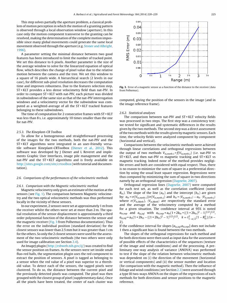
In our experiment, 2 sensors were set at approximately 1 m fromhe receiver whilst the others were set at more than 2 m. The spa-ial resolution of the sensor displacement is approximately a thirdrder polynomial function of the distance between the sensor andhe magnetic receiver (Fig. 3 from Polhemus documentation). Thushe error on the individual position (standard deviation) for thelosest sensors was lower than 2.5 mm but it was greater than 1 cmor the others. So only the 2 closest sensors were used for the assess-

ent of the two velocimetric methods (the two others were onlysed for image calibration see Section 2.4).

An ImageJ plugin (http://rsbweb.nih.gov/ij/) was created to findhe sensor position on frames. As the sensors were set inside smalluo-red balls, the segmentation plugin uses the red component toxtract the position of sensors. A pixel is tagged as belonging to

sensor when the red value of a pixel was superior to a thresh-ld value. To detect each of the sensors, the tagged pixels were

lustered. To do so, the distance between the current pixel andhe previously detected pixels was computed. The pixel was thenrouped with the closest group of pixel (supplementary data). Oncell the pixels have been treated, the center of each cluster was

Fig. 3. Error of a magnetic sensor as a function of the distance to the receiver (datafrom Polhemus).

computed, giving the position of the sensors in the image (and inthe image reference frame).

2.6.2. Statistical analysesThe comparison between nat-PIV and ST + KLT velocity fields

was processed in two steps. The first step was a consistency test:we tested for significant and systematic differences in the resultsgiven by the two methods. The second step was a direct assessmentof the two methods with the results given by magnetic sensors. Eachtime, the velocity fields were analyzed component by component(horizontal and vertical).

Comparisons between the velocimetric methods were achievedthrough linear correlations and orthogonal regressions betweenthe output of two methods Vts,meth-i = f(Vts,meth-j) (i.e. nat-PIV vsST + KLT, and then nat-PIV vs magnetic tracking and ST + KLT vsmagnetic tracking. Indeed none of the method provides negligi-ble errors and both are considered with equal respect. Thus, thereis no reason to minimize the sum of square in a preferential direc-tion by using the usual least square regression. Regressions werethus computed by minimizing the sum of square in two directionsnamely by an orthogonal regression (Dagnelie, 2007).

Orthogonal regression lines (Dagnelie, 2007) were computedfor each test set, as well as the correlation coefficient (notedRts). The slope of the line (ats) and the intercept (bts) are givenby: ats = �(Vts,meth-i)/�(Vts,meth-j) and bts = 〈Vts,meth-i〉 − ats 〈Vts,meth-j〉where �(Vts,Meth), 〈Vts,Meth〉 are respectively the standard errorand the average of the velocimetry computed by a methodfor a given situation. The confidence interval at 95% is notedats,sup and ats,inf with ats,sup = ats(1 + 2kts + ((1 + 2kts)2 − 1)1/2)1/2,ats,inf = ats(1 + 2kts − ((1 + 2kts)2 − 1)1/2)1/2, k = t2

1−˛/2(1 − R2ts)/(n −

2).If the confidence interval for slopes [ats,inf,ats,sup] does not include1 then a significant bias is found between the two methods.

The slopes of the orthogonal regressions for each method andfor both directions were then used as input data for the assessmentof possible effects of the characteristics of the sequences (textureof the image and wind conditions) and of the processing. A pre-liminary one-way analysis of variance (ANOVA) was performedto test if the slope of the relation between velocimetric methodswas dependent on (i) the direction of the movement (horizontalor vertical components) and (ii) the sensor number and location(for comparison with the magnetic method). Then the influence of

foliage and wind conditions (see Section 2.3) were assessed througha type III two-ways ANOVA on the slopes of the regressions of eachmethods for both directions and sensor positions to the magneticreference.

226 A. Barbacci et al. / Agricultural and Forest Meteorology 184 (2014) 220– 229

Fig. 4. Illustration of velocimetry fields for the situation DHighW (Dense foliage et High wind velocimetry) for nat-PIV and ST + KLT methods.

F for tb

sS

3

3

tS

tost

TRs

ig. 5. Comparison between displacement fields computed by nat-PIV and ST + KLTy ST + KLT. �c is the sampling time of the camera (�c = 1/25 s).

All the statistical computations were made with MATLAB ver-ion 7.10.0 (Natick, Massachusetts: The MathWorks Inc., 2010,tatistics toolbox).

. Result

.1. Comparison nat-PIV/ST + KLT

Fig. 4 displays typical instantaneous velocity fields obtained forhe Dense Foliage and high wind conditions, using both nat-PIV andT + KLT (see also supplementary data).

In both cases the velocity fields described only the motion of the

ree elements, and not of the background (e.g. clouds). The densityf the velocity field was high, but not homogeneous, displayingome patchiness (with a slightly more pronounced patchiness forhe output of ST + KLT). For both methods the central zone of the

able 2esult of the orthogonal regressions for each velocimetry direction for the relation betwlopes; bts = Y-intercept and Rts = correlation coefficient).

Test-set Horizontal

ats ats− ats+ bts R

DHighW 0.8448 0.8445 0.8452 0.006 0DMediumW 0.8756 0.8752 0.8759 0.004 0IHighW 0.8157 0.8154 0.8160 0.004 0IMediumW 0.7124 0.7121 0.7127 −0.004 0

wo test sets. The velocity computed by nat-PIV is superior than the one computed

crown displayed a lower density in the velocity field. There weresome “black patches” where no velocity estimates were found, butthese “black patches” were of limited extent. nat-PIV tended to out-put some surprisingly large velocity vectors at the boundaries of thecrown (outliers), whereas ST + KLT did not.

The result of the orthogonal regression of the relationVts,ST+KLT = f(Vts,nat-PIV) were qualitatively the same for all the testsets (Fig. 5 and Table 2). There was a good linear correlationbetween the outputs of the two methods, with normally distributedresidual errors. However this correlation and the explained vari-ance tended to be weaker for the vertical components of thevelocity vectors than for the horizontal components. Moreover,

the slopes were systematically significantly inferior to 1 whilethe Y-intercept of the regression was always quite close to 0 (nosystematic bias). So, the velocities computed by ST + KLT were sys-tematically smaller than the ones computed by nat-PIV.

een nat-PIV and ST + KLT (ats = slope; ats− ats+ = limits of the confidence interval on

Vertical

2ts ats ats− ats+ bts R2

ts

.72 0.8216 0.8212 0.8220 0.008 0.62

.72 0.8622 0.8618 0.8626 0.003 0.59

.69 0.8037 0.8033 0.8040 0.003 0.57

.46 0.7089 0.7085 0.7092 0.003 0.42

A. Barbacci et al. / Agricultural and Forest Meteorology 184 (2014) 220– 229 227

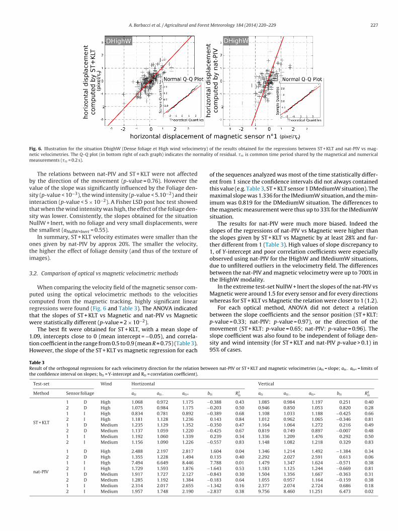
F etry) on rmalitm

bvsitsNt

oti

3

pcrtw

1tH

TRt

ig. 6. Illustration for the situation DhighW (Dense foliage et High wind velocimetic velocimetries. The Q–Q plot (in bottom right of each graph) indicates the noeasurements (�rs = 0.2 s).

The relations between nat-PIV and ST + KLT were not affectedy the direction of the movement (p-value = 0.76). However thealue of the slope was significantly influenced by the Foliage den-ity (p-value < 10−3), the wind intensity (p-value < 5.10−2) and theirnteraction (p-value < 5 × 10−2). A Fisher LSD post hoc test showedhat when the wind intensity was high, the effect of the foliage den-ity was lower. Consistently, the slopes obtained for the situationullW + Inert, with no foliage and very small displacements, were

he smallest (aNullW+Inert = 0.55).In summary, ST + KLT velocity estimates were smaller than the

nes given by nat-PIV by approx 20%. The smaller the velocity,he higher the effect of foliage density (and thus of the texture ofmages).

.2. Comparison of optical vs magnetic velocimetric methods

When comparing the velocity field of the magnetic sensor com-uted using the optical velocimetric methods to the velocitiesomputed from the magnetic tracking, highly significant linearegressions were found (Fig. 6 and Table 3). The ANOVA indicatedhat the slopes of ST + KLT vs Magnetic and nat-PIV vs Magneticere statistically different (p-value = 2 × 10−2).

The best fit were obtained for ST + KLT, with a mean slope of.09, intercepts close to 0 (mean intercept = −0.05), and correla-ion coefficient in the range from 0.5 to 0.9 (mean R = 0.75) (Table 3).owever, the slope of the ST + KLT vs magnetic regression for each

able 3esult of the orthogonal regressions for each velocimetry direction for the relation betwhe confidence interval on slopes; bts = Y-intercept and Rts = correlation coefficient).

Test-set Wind Hortizontal

Method Sensor foliage ats ats− ats+ b

ST + KLT

1 D High 1.068 0.972 1.175 −2 D High 1.075 0.984 1.175 −1 I High 0.834 0.781 0.892 −2 I High 1.181 1.128 1.236

1 D Medium 1.235 1.129 1.352 −2 D Medium 1.137 1.059 1.220 −1 I Medium 1.192 1.060 1.339

2 I Medium 1.156 1.090 1.226 −

nat-PIV

1 D High 2.488 2.197 2.817

2 D High 1.355 1.228 1.494

1 I High 7.494 6.649 8.446

2 I High 1.729 1.593 1.876 −1 D Medium 1.917 1.727 2.127 −2 D Medium 1.285 1.192 1.384 −1 I Medium 2.314 2.017 2.655 −2 I Medium 1.957 1.748 2.190 −

f the results obtained for the regressions between ST + KLT and nat-PIV vs mag-y of residual. �rs is common time period shared by the magnetical and numerical

of the sequences analyzed was most of the time statistically differ-ent from 1 since the confidence intervals did not always containedthis value (e.g. Table 3, ST + KLT sensor 1 DMediumW situation). Themaximal slope was 1.336 for the IMediumW situation, and the min-imum was 0.819 for the DMediumW situation. The differences tothe magnetic measurement were thus up to 33% for the IMediumWsituation.

The results for nat-PIV were much more biased. Indeed theslopes of the regressions of nat-PIV vs Magnetic were higher thanthe slopes given by ST + KLT vs Magnetic by at least 28% and fur-ther different from 1 (Table 3). High values of slope discrepancy to1, of Y-intercept and poor correlation coefficients were especiallyobserved using nat-PIV for the IHighW and IMediumW situations,due to unfiltered outliers in the velocimetry field. The differencesbetween the nat-PIV and magnetic velocimetry were up to 700% inthe IHighW modality.

In the extreme test-set NullW + Inert the slopes of the nat-PIV vsMagnetic were around 1.5 for every sensor and for every directionswhereas for ST + KLT vs Magnetic the relation were closer to 1 (1.2).

For each optical method, ANOVA did not detect a relationbetween the slope coefficients and the sensor position (ST + KLT:p-value = 0.33; nat-PIV: p-value = 0.97), or the direction of themovement (ST + KLT: p-value = 0.65; nat-PIV: p-value = 0.96). The

slope coefficient was also found to be independent of foliage den-sity and wind intensity (for ST + KLT and nat-PIV p-value > 0.1) in95% of cases.

een nat-PIV or ST + KLT and magnetic velocimetries (ats = slope; ats− ats+ = limits of

Vertical

ts R2ts ats ats− ats+ bts R2

ts

0.388 0.43 1.085 0.984 1.197 0.251 0.400.203 0.50 0.946 0.850 1.053 0.820 0.280.389 0.68 1.108 1.033 1.188 −0.425 0.660.143 0.84 1.012 0.962 1.065 −0.346 0.810.350 0.47 1.164 1.064 1.272 0.216 0.490.425 0.67 0.819 0.749 0.897 −0.007 0.480.239 0.34 1.336 1.209 1.476 0.292 0.500.557 0.83 1.148 1.082 1.218 0.329 0.83

1.604 0.04 1.346 1.214 1.492 −1.384 0.340.135 0.40 2.292 2.027 2.591 0.613 0.067.788 0.01 1.479 1.347 1.624 −0.571 0.381.643 0.53 1.183 1.125 1.244 −0.669 0.810.843 0.30 1.504 1.356 1.667 −0.363 0.310.183 0.64 1.055 0.957 1.164 −0.159 0.381.342 0.16 2.377 2.074 2.724 0.686 0.182.837 0.38 9.756 8.460 11.251 6.473 0.02

2 Forest

4

emuwcastc(e

rscbtatqh

bte(fiw

wdMrstpop

jwlfwcolicBftpdmitttmum(

28 A. Barbacci et al. / Agricultural and

. Discussion and conclusion

These experiments demonstrate that reliable and consistentstimates of dense velocity fields resulting from wind-inducedotions of complex trees in natural conditions can be achieved

sing video recording by standard cameras, in all the situations ofind and foliage density. This was achieved in a very challenging

onditions, namely a complex tree in the field, with natural lightingnd changing sky background, in a sample of different weathers andeasonal foliage situations all through the year. To our knowledgehis is the very first time that these methods have been systemati-ally assessed versus a reference method for plants measurementsaccuracy assessment have been performed but on simple scenes,.g. Westerweel, 2000).

The ST + KLT method proved to always be more accurate andobust. This could not be inferred from theory. Indeed the mosttraightforward hypothesis was that nat-PIV would be more effi-ient for dense foliages, and that the ST + KLT method would onlye efficient with obvious angular features such as in the leaflessree. But this is not the case. Even in conditions of dense foliage,

high density of “good features to track” were found (mostly leafips, bases, etc.) using ST. The ST + KLT method also proved to beuite insensitive to possible light intensity gradients set up by theeterogeneous lighting intrinsic to natural light conditions.

It may be argued that part of the behavior of the nat-PIV coulde improved by using more advanced post-processing filtering thanhe standard one we used in this study (e.g. Vétel et al., 2011). How-ver most of the aberrant vectors were lying at the edge of the fieldi.e. edge of the crown), and this is the most difficult situation forltering. Therefore a method that provides more consistent outputsithout filtering (as does the ST + KLT) is to be preferred.

Although providing on average a non-biased estimates, ST + KLTas found to provide possible errors up to 20% along horizontalirection and up to 33% along vertical one (when compared toagnetic tracking). The reason for this is not clear, and did not

elate to any of the studied factors (wind intensity, foliage den-ity, motion direction). However this drawback is compensated forhe advantages of the ST + KLT optical velocimetric method, com-ared to contact methods such as magnetic tracking, inclinometerr strain gauges. Indeed none of the contact methods is able toroduce such a dense field of velocity.

This study was however dedicated to the analysis of the 2D pro-ection of the wind-induced motion of an isolated tree. Moreover,

e studied cases in which the direction of the dominant wind wasaying along the image, so that the drag motion should be easier toollow. Producing a 3D reconstruction of the velocity field for anyind direction is theoretically possible, but will face the usual diffi-

ulties of 3D reconstruction of trees, namely the automatic pairingf the features to track, and the problem of hidden objects. It isikely that the result will be less dense and noisier. If the wind-nduced tree motions are the main target though, an alternativean be to identify vibration modes of the tree (using for examplei Orthogonal Decomposition, e.g. Py et al., 2006) on the videos

rom two orthogonal cameras. Instead of matching the good fea-ure to track one by one, the whole vibration modes in the twolanes can be matched from their frequency and the global modaleformation then reconstructed. This may allow identifying branchodes, but also the modes involving the deformation of the trunk,

n which all the points in the crown experience a coherent motion,o be reconstructed (see Rodriguez et al., 2008 for the descrip-ion and typology of vibration modes in a walnut tree). Howeverhe direct measurement of the trunk through local measurements

ethods (displacement sensors, tilt meters, strain gauges, etc.) aresually easy, and will provide accurate description of the defor-ation of stem and main branches. So the two types of methods

optical ST + KLT velocimetry and local measurements) can easily be

Meteorology 184 (2014) 220– 229

associated to provide an accurate and dense description of themotion and deformation of the whole tree.

A further complication may be experienced when trying to ana-lyze plants within a dense canopy. The drawbacks here are those ofany optical method (hidden parts, obstacles to step back the cam-eras, etc.). Optical methods may however been used to track themotion of the top of the canopy, as long as it produces a fairly flatsurface (crop and grasses, young forests). Py et al. (2005, 2006) haveused nat-PIV in these conditions, providing novel insights on theplant–wind interactions on top of the canopy. However their vali-dation was crude. It is likely that they would have experienced thebias that was revealed in that study and the ST + KLT method islikely to be more reliable in these situations.

Finally, although we experienced very different cloudiness alongthe experiment (see Fig. 1), we cannot claimed to have investigatedall the type of background. In the case of moving background (e.g.small clouds) though, the Kineplant-CRToolbox software providestools to restrict the part of the image used to compute velocimetryfields to the vicinity of the tree. This can achieved either manuallyor automatically.

The ST + KLT method and the Kineplant-CRToolbox softwarethus provide a reliable and straightforward method for densevelocimetric measurements of wind induced movement. It isnow available for use by plant biomechanics, micrometerology ormechanobiology. This should allow for developments in the exper-imental study of wind induced motion, and to the possibility ofassessing models of plant–wind interaction. Finally the dataset pro-duced of tree and wind velocities during this experiment is uniqueand may be used to assess mechanical models of wind–tree inter-actions with explicit architecture (e.g. Sellier et al., 2006; Rodriguezet al., 2008). Data are available on request by e-mail.

Acknowledgments

The authors wish to thanks the anonymous reviewers for theirrelevant remarks and comments.

This work was supported by ANR Grant 06-BLAN-0210-02“Chêne Roseau” involving the Ecole Polytechnique, INRIA and INRA.The authors thank S. Ploquin and P. Chaleil for technical assistancewith the tree experiments.

Appendix A. Supplementary data

Supplementary data associated with this article can be found,in the online version, at http://dx.doi.org/10.1016/j.agrformet.2013.10.003.

References

Achim, A., Ruel, J., Gardiner, B., Laflamme, G., Meunier, S., 2005. Modelling the vul-nerability of balsam fir forests to wind damage. Forest Ecol. Manage. 204, 37–52.

Baker, S., Matthews, I., 2004. Lucas-Kanade 20 years on: a unifying framework. Int.J. Comput. Vis. 56, 221–255.

Berry, P., Sterling, M., Baker, C.J., Spink, J., Sparkes, D.L., 2003. A calibrated modelof wheat lodging compared with field measurements. Agric. For. Meteorol. 119,167–180.

Bouguet, J.-Y., 2000. Pyramidal Implementation of the Lucas Kanade FeatureTracker Description of the algorithm. http://robots.stanford.edu/cs223b04/algo tracking.pdf

Bradski, G., 2000. The OpenCV Library. Dr. Dobb’s Journal of Software Tools.Carr, Z.R., Ahmed, K.A., Forliti, D.J., 2009. Spatially correlated precision error in digital

particle image velocimetry measurements of turbulent flows. Exp. Fluids 47,95–106.

Cholemari, M.R., 2007. Modeling and correction of peak-locking in digital PIV. Exp.Fluids 42, 913–922.

Christensen, K.T., 2004. The influence of peak-locking errors on turbulence statistics

computed from PIV ensembles. Exp. Fluids 36, 484–497.

Dagnelie, P., 2007. Statistique théorique et appliquée. Tome 1. Statistique descriptiveet bases de l’inférence statistique. Bruxelles, De Boeck et Larcier.

de Langre, E., 2006. Frequency lock-in is caused by coupled-mode flutter. J. FluidsStruct. 22, 783–791.

Forest

dd

D

D

D

D

D

F

F

G

G

HH

H

L

L

M

MBot. 93 (10), 1466–1476.

A. Barbacci et al. / Agricultural and

e Langre, E., 2008. Effects of wind on plants. Ann. Rev. Fluid Mech. 40, 141–168.e Langre, E., Rodriguez, M., Ploquin, S., Moulia, B., 2012. The multimodal dynamics

of a walnut tree: experiments and models. J. Appl. Mech. 79 (4).iener, J., Reveret, L., Fiume, E., 2006. Hierarchical retargetting of 2D motion fields to

the animation of 3D plant models. In: ACM SIGGRAPH/Eurographics Symposiumon Computer Animation, SCA’06, September 2–4, Vienna, Austria.

iener, J., Barbacci, A., Hemon, P., de Langre, E., Moulia, M., 2012. CR – KinePlanttoolbox. In: Proceedings of the 7th International Biomechanics Conference,Clermont-Ferrand, p. 179.

onès, N., Adam, B., 2008. PiafDigitTrack -Software to drive a Polhemus Fastrak 3SPACE 3D digitiser and for the acquisition of plant architecture. In: UMR PIAFINRA-UBP Clermont-Ferrand.

upont, S., Brunet, Y., 2007. Edge flow and canopy structure: a large-eddy simulationstudy. Boundary Layer Meteorol. 126, 51–71.

upont, S., Gosselin, F., Py, C., de Langre, E., Hemon, P., Brunet, Y., 2010. Modelingwaving crops using large-eddy simulation: comparison with experiments and alinear stability analysis. J. Fluid Mech. 652, 5–44.

lesch, T.K., Grant, R.H., 1992a. Corn motion in the wind during senescence: I. Motioncharacteristics. Agron. J. 84, 748–751.

lesch, T.K., Grant, R.H., 1992b. Corn motion in the wind during senescence: II. Effectof dynamic plant characteristics. Agron. J. 84, 742–747.

ardiner, B., 2000. Comparison of two models for predicting the critical wind speedsrequired to damage coniferous trees. Ecol. Modell. 129, 1–23.

ardiner, B., Byrne, K., Hale, S., Kamimura, K., Mitchell, S.J., Peltola, H., Ruel, J.C., 2008.A review of mechanistic modelling of wind damage risk to forests. Forestry 81(3), 447–463.

orn, B.K.P., Schunck, B.G., 1981. Determining optical flow. Artif. Intell. 17, 185–203.edden, R.L., Fredericksen, T.S., Williams, S.A., 1995. Modelling the effect of crown

shedding and streamlining on the survival of loblolly pine exposed to acutewind. Can. J. For. Res. 25, 704–712.

assinen, A., Lemettinen, M., Peltola, H., Kellomäki, S., Gardiner, B., 1998. A prism-based system for monitoring the swaying of trees under wind loading. Agric.Forest Meteorol. 90 (3), 187–194.

ucas, B., Kanade, T., 1981. An iterative image registration technique with an appli-cation to stereo vision. In: Proceedings of the Imaging Understanding Workshop,pp. 121–130.

opez, D., Michelin, S., de Langre, E., 2011. Flow-induced pruning of branched sys-tems and brittle reconfiguration. J. Theor. Biol. 284 (1), 117–124.

oulia, B., Fournier, M., 1997. Mechanics of the maize leaf: a composite beam modelof the midrib. J. Mater. Sci. 32, 2771–2780.

oulia, B., Der Loughian, C., Bastien, R., Martin, L., Rodríguez, M., Gourcilleau, D., Bar-bacci, A., Badel, E., Franchel, J., Lenne, C., Roeckel-Drevet, P., Allain, J.M., Frachisse,J.M., de Langre, E., Coutand, C., Fournier-Leblanc, N., Julien, J.L., 2011. Mechan-ical integration of plant cells and plants. In: Wojtaszek, P. (Ed.), MechanicalIntegration of Plant Cells and Plants. Springer, Berlin, Heidelberg, pp. 269–302.

Meteorology 184 (2014) 220– 229 229

Niklas, K.J., Spatz, H.-C., 2000. Wind-induced stresses in cherry trees: evidenceagainst the hypothesis of constant stress levels. Trees Struct. Funct. 14,230–237.

Py, C., de Langre, E., Moulia, B., Hemon, P., 2005. Measurement of wind-inducedmotion of crop canopies from digital video images. Agric. For. Meteorol. 130,223–236.

Py, C., de Langre, E., Moulia, B., 2006. A frequency lock-in mechanism in the interac-tion between wind and crop canopies. J. Fluid Mech. 568, 425–449.

Raffel, M., Willert, C., Kompenhans, J., 2002. Particle Image Velocimetry: A PracticalGuide, 1st ed. Springer, 1998, Corr. 2nd printing edition (Jun 11, 2002).

Raupach, M.R., Finnigan, J.J., Brunei, Y., 1996. Coherent eddies and turbulence invegetation canopies: the mixing-layer analogy. Boundary Layer Meteorol. 78,351–382.

Rudnicki, M., Silins, U., Lieffers, V.J., Josi, G., 2001. Measure of simultaneous treesways and estimation of crown interactions among a group of trees. Trees 15,83–90.

Rudnicki, M., Burns, D., 2006. Branch sway period of four tree species using 3dmotion tracking. In: Proceedings of the 5th Plant Biomechanics Conference,pp. 25–31.

Rodriguez, M., Langre, E.D., Moulia, B., 2008. A scaling law for the effects of archi-tecture and allometry on tree vibration modes suggests a biological tuning tomodal compartmentalization. Am. J. Bot. 95, 1523–1537.

Rodriguez, M., Ploquin, S., Moulia, B., de Langre, E., 2012. The multimodal dynam-ics of a walnut tree: experiments and models. J. Appl. Mech. Trans. ASME79 (4).

Sellier, D., Fourcaud, T., Lac, P., 2006. A finite element model for investigating effectsof aerial architecture on tree oscillations. Tree Physiol. 26, 799–806.

Sellier, D., Fourcaud, T., 2005. A mechanical analysis of the relationship betweenfree oscillations of Pinus pinaster Ait. saplings and their aerial architecture. TreePhysiol. 56 (416), 1563–1573.

Shi, J., Tomasi, C., 1994. Good features to track. In: Proceedings of IEEE Conferenceon Computer Vision and Pattern Recognition:, pp. 593–600.

Sterling, M., Baker, C.J., Berry, P.M., Wade, A., 2003. An experimental investigationof the lodging of wheat. Agric. Forest Meteorol. 119, 149–165.

Stoner, G.R., Albright, T.D., 1996. The interpretation of visual motion: evidence forsurface segmentation mechanisms. Vis. Res. 36, 1291–1310.

Sveen, J.K., 2004. An introduction to MatPIV v.1.6.1. World Wide Web Internet AndWeb Information Systems.

Telewski, F.W., 2006. A unified hypothesis of mechanoperception in plants. Am. J.

Vétel, J., Garon, A., Pelletier, P., 2011. Denoising methods for time-resolved PIV mea-surements. Exp. Fluids 51, 893–916.

Westerweel, J., 2000. Theoretical analysis of the measurement precision in particleimage velocimetry. Exp. Fluids, 3–12.