Multi-Level Steiner Trees - arXiv

Multi-Level Steiner Trees

REYAN AHMED, University of Arizona, USA

PATRIZIO ANGELINI, Universität Tübingen, Germany

FARYAD DARABI SAHNEH, University of Arizona, USA

ALON EFRAT, University of Arizona, USA

DAVID GLICKENSTEIN, University of Arizona, USA

MARTIN GRONEMANN, Universität zu Köln, Germany

NIKLAS HEINSOHN, Universität Tübingen, Germany

STEPHEN G. KOBOUROV, University of Arizona, USA

RICHARD SPENCE, University of Arizona, USA

JOSEPH WATKINS, University of Arizona, USA

ALEXANDER WOLFF, Universität Würzburg, Germany

In the classical Steiner tree problem, given an undirected, connected graphG = (V ,E) with non-negative edge

costs and a set of terminals T ⊆ V , the objective is to find a minimum-cost tree E ′ ⊆ E that spans the terminals.

The problem is APX-hard; the best known approximation algorithm has a ratio of ρ = ln(4) + ε < 1.39. In this

paper, we study a natural generalization, the multi-level Steiner tree (MLST) problem: given a nested sequence

of terminalsTℓ ⊂ · · · ⊂ T1 ⊆ V , compute nested trees Eℓ ⊆ · · · ⊆ E1 ⊆ E that span the corresponding terminal

sets with minimum total cost.

The MLST problem and variants thereof have been studied under various names including Multi-level

Network Design, Quality-of-Service Multicast tree, Grade-of-Service Steiner tree, and Multi-Tier tree. Several

approximation results are known. We first present two simple O(ℓ)-approximation heuristics. Based on

these, we introduce a rudimentary composite algorithm that generalizes the above heuristics, and determine

its approximation ratio by solving a linear program. We then present a method that guarantees the same

approximation ratio using at most 2ℓ Steiner tree computations. We compare these heuristics experimentally

on various instances of up to 500 vertices using three different network generation models. We also present

various integer linear programming (ILP) formulations for the MLST problem, and compare their running

times on these instances. To our knowledge, the composite algorithm achieves the best approximation ratio

for up to ℓ = 100 levels, which is sufficient for most applications such as network visualization or designing

multi-level infrastructure.

Additional Key Words and Phrases: Approximation algorithm; Steiner tree; multi-level graph representation.

Authors’ addresses: Reyan Ahmed, University of Arizona, Tucson, AZ, USA, [email protected]; Pa-

trizio Angelini, Universität Tübingen, Tübingen, Germany; Faryad Darabi Sahneh, University of Arizona, Tucson, AZ, USA,

[email protected]; Alon Efrat, University of Arizona, Tucson, AZ, USA, [email protected]; David Glickenstein,

University of Arizona, Tucson, AZ, USA, [email protected]; Martin Gronemann, Universität zu Köln, Cologne,

Germany, [email protected]; Niklas Heinsohn, Universität Tübingen, Tübingen, Germany, heinsohn@

informatik.uni-tuebingen.de; Stephen G. Kobourov, University of Arizona, Tucson, AZ, USA, [email protected];

Richard Spence, University of Arizona, Tucson, AZ, USA, [email protected]; Joseph Watkins, University of

Arizona, Tucson, AZ, USA, [email protected]; Alexander Wolff, Universität Würzburg, Würzburg, Germany.

Permission to make digital or hard copies of all or part of this work for personal or classroom use is granted without fee

provided that copies are not made or distributed for profit or commercial advantage and that copies bear this notice and

the full citation on the first page. Copyrights for components of this work owned by others than ACM must be honored.

Abstracting with credit is permitted. To copy otherwise, or republish, to post on servers or to redistribute to lists, requires

prior specific permission and/or a fee. Request permissions from [email protected].

© 2018 Association for Computing Machinery.

1084-6654/2018/11-ART $15.00

https://doi.org/10.1145/nnnnnnn.nnnnnnn

ACM J. Exp. Algor., Vol. 1, No. 1, Article . Publication date: November 2018.

arX

iv:1

804.

0262

7v2

[cs

.DS]

26

Nov

201

8


2 R. Ahmed et al.

ACM Reference Format:Reyan Ahmed, Patrizio Angelini, Faryad Darabi Sahneh, Alon Efrat, David Glickenstein, Martin Gronemann,

Niklas Heinsohn, Stephen G. Kobourov, Richard Spence, Joseph Watkins, and Alexander Wolff. 2018. Multi-

Level Steiner Trees. ACM J. Exp. Algor. 1, 1 (November 2018), 22 pages. https://doi.org/10.1145/nnnnnnn.

nnnnnnn

ACKNOWLEDGMENTSThis work is partially supported by NSF grants CCF-1423411 and CCF-1712119.

The authors wish to thank the organizers and participants of the First Heiligkreuztal Workshop

on Graph and Network Visualization where work on this problem began.

1 INTRODUCTIONLet G = (V ,E) be an undirected, connected graph with positive edge costs c : E → R+, and let

T ⊆ V be a set of vertices called terminals. A Steiner tree is a tree in G that spans T . The network(graph) Steiner tree problem (ST) is to find a minimum-cost Steiner tree E ′ ⊆ E, where the cost of E ′

is c(E ′) = ∑e ∈E′ c(e). ST is one of Karp’s initial NP-hard problems [12]; see also a survey [21], an

online compendium [11], and a textbook [18].

Due to its practical importance in many domains, there is a long history of exact and approxi-

mation algorithms for the problem. The classical 2-approximation algorithm for ST [10] uses the

metric closure of G , i.e., the complete edge-weighted graph G∗with vertex set T in which, for every

edge uv , the cost of uv equals the length of a shortest u–v path in G. A minimum spanning tree

of G∗corresponds to a 2-approximate Steiner tree in G.

Currently, the last in a long list of improvements is the LP-based approximation algorithm

of Byrka et al. [5], which has a ratio of ln(4) + ε < 1.39. Their algorithm uses a new iterative

randomized rounding technique. Note that ST is APX-hard [4]; more concretely, it is NP-hard to

approximate the problem within a factor of 96/95 [7]. This is in contrast to the geometric variant

of the problem, where terminals correspond to points in the Euclidean or rectilinear plane. Both

variants admit polynomial-time approximation schemes (PTAS) [1, 15], while this is not true for

the general metric case [4].

In this paper, we consider the natural generalization of ST where the terminals appear on “levels”

(or “grades of service”) and must be connected by edges of appropriate levels. We propose new

approximation algorithms and compare them to existing ones both theoretically and experimentally.

Definition 1.1 (Multi-Level Steiner Tree (MLST) Problem). Given a connected, undirected graph

G = (V ,E) with edge weights c : E → R+ and ℓ nested terminal sets Tℓ ⊂ · · · ⊂ T1 ⊆ V , amulti-level Steiner tree consists of ℓ nested edge sets Eℓ ⊆ · · · ⊆ E1 ⊆ E such that Ei spans Ti forall 1 ≤ i ≤ ℓ. The cost of an MLST is defined by the sum of the edge weights across all levels,∑ℓ

i=1 c(Ei ) =∑ℓ

i=1∑

e ∈Ei c(e). The MLST problem is to find an MLST EOPT, ℓ ⊆ · · · ⊆ EOPT,1 ⊆ Ewith minimum cost.

Since the edge sets are nested, the cost of an MLST equivalently equals

∑e ∈E L(e)c(e), where

L(e) denotes the highest level that edge e appears in, where L(e) = 0 if e < E1. This emphasizes that

the cost of each edge is multiplied by the number of levels it appears on.

We denote the cost of an optimal MLST by OPT. We can write

OPT = ℓOPTℓ + (ℓ − 1)OPTℓ−1 + · · · + OPT1

where OPTℓ = c(EOPT, ℓ) and OPTi = c(EOPT,i\EOPT,i+1) for ℓ − 1 ≥ i ≥ 1. Thus OPTi represents

the cost of edges on level i but not on level i + 1 in the minimum cost MLST. Figure 1 shows an

example of an MLST for ℓ = 3.




Multi-Level Steiner Trees 3

Fig. 1. An illustration of an MLST with ℓ = 3 for the graph at the right. Solid and open circles represent

terminal and non-terminal nodes, respectively. Note that the level-3 tree (left) is contained in the level-2 tree

(mid), which is in turn contained in the level-1 tree (right).

Applications. This problem has natural applications in designing multi-level infrastructure of

low cost. Apart from this application in network design, multi-scale representations of graphs are

useful in applications such as network visualization, where the goal is to represent a given graph

at different levels of detail.

PreviousWork. Variants of the MLST problem have been studied previously under various names,

such asMulti-Level Network Design (MLND) [2],Multi-Tier Tree (MTT) [14], Quality-of-Service (QoS)Multicast Tree [6], and Priority-Steiner Tree [8].

In MLND, the vertices of the given graph are partitioned into ℓ levels, and the task is to constructan ℓ-level network. Each edge (i, j) ∈ E can contain one of ℓ different facility types (levels), each

with a different cost (denoted “secondary” and “primary” with costs 0 ≤ bi j ≤ ai j for 2 levels).

The vertices on each level must be connected by edges of the corresponding level or higher, and

edges of higher level are more costly. The cost of an edge partition is the sum of all edge costs,

and the task is to find a partition of minimum cost. Let ρ be the ratio of the best approximation

algorithm for (single-level) ST, that is, currently ρ = ln(4) + ε < 1.39. Balakrishnan et al. [2] gave

a (4/3)ρ-approximation algorithm for 2-level MLND with proportional edge costs. Note that the

definitions of MLND and MLST treat the bottom level differently. While MLND requires that allvertices are connected eventually, this is not the case for MLST.

For MTT, which is equivalent to MLND, Mirchandani [14] presented a recursive algorithm

that involves 2ℓSteiner tree computations. For ℓ = 3, the algorithm achieves an approximation

ratio of 1.522ρ independently of the edge costs c1, . . . , cℓ : E → R+. For proportional edge costs,Mirchandani’s analysis yields even an approximation ratio of 1.5ρ for ℓ = 3. Recall, however, that

this assumes T1 = V , and setting the edge costs on the bottom level to zero means that edge costs

are not proportional.In the QoSMulticast Tree problem [6] one is given a graph, a source vertex s , and a level between 1

and k for each terminal (1 for highest priority). The task is to find a minimum-cost Steiner tree that

connects all terminals to s . The level of an edge e in this tree is the minimum over the levels of

the terminals that are connected to s via e . The cost of the edges and of the tree are as above. As

a special case, Charikar et al. [6] studied the rate model, where edge costs are proportional, andshow that the problem remains NP-hard if all vertices (except the source) are terminals (at some

level). Note that if we choose as source any vertex at the top level Tℓ , then MLST can be seen as an

instance of the rate model.

Charikar et al. [6] gave a simple 4ρ-approximation algorithm for the rate model. Given an

instance φ, their algorithm constructs an instance φ ′where the levels of all vertices are rounded up

to the nearest power of 2. Then the algorithm simply computes a Steiner tree at each level of φ ′and

prunes the union of these Steiner trees into a single tree. The ratio can be improved to eρ, where eis the base of the natural logarithm, using randomized doubling.

Instead of taking the union of the Steiner trees on each rounded level, Karpinski et al. [13]

contract them into the source in each step, which yields a 2.454ρ-approximation. They also gave a

(1.265 + ε)ρ-approximation for the 2-level case. (Since these results are not stated with respect to ρ,


4 R. Ahmed et al.

but depend on several Steiner tree approximation algorithms – among them the best approximation

algorithm with ratio 1.549 [19] available at the time – we obtained the numbers given here by

dividing their results by 1.549 and stating the factor ρ.)For the more general Priority-Steiner Tree problem, where edge costs are not necessarily pro-

portional, Charikar et al. [6] gave a min{2 ln |T |, ℓρ}-approximation algorithm. Chuzhoy et al. [8]

showed that Priority-Steiner Tree does not admit an O(log logn)-approximation algorithm unless

NP ⊆DTIME(nO (log log logn)). For Euclidean MLST, Xue at al. [22] gave a recursive algorithm that

uses any algorithm for Euclidean Steiner Tree (EST) as a subroutine. With a PTAS [1, 15] for EST,

the approximation ratio of their algorithm is 4/3 + ε for ℓ = 2 and (5 + 4√2)/7 + ε ≈ 1.522 + ε for

ℓ = 3.

Our Contribution. We give two simple approximation algorithms for MLST, bottom-up and

top-down, in Section 2.1. The bottom-up heuristic uses a Steiner tree at the bottom level for the

higher levels after pruning unnecessary edges at each level. The top-down heuristic first computes

a Steiner tree on the top level. Then it passes edges down from level to level until the bottom level

terminals are spanned.

In Section 2.2, we propose a composite heuristic that generalizes these, by examining all possible

2ℓ−1

(partial) top-down and bottom-up combinations and returning the one with the lowest cost.

We propose a linear program that finds the approximation ratio of the composite heuristic for any

fixed value of ℓ, and compute approximation ratios for up to ℓ = 100 levels, which turn out to

be better than those of previously known algorithms. However, the composite heuristic requires

roughly 2ℓℓ ST computations.

Therefore, we propose a procedure that achieves the same approximation ratio as the composite

heuristic but needs at most 2ℓ ST computations. In particular, it achieves a ratio of 1.5ρ for ℓ = 3

levels, which settles a question posed by Karpinski et al. [13] who were asking whether the

(1.522 + ε)-approximation of Xue at al. [22] can be improved for ℓ = 3. Note that Xue et al. treated

the Euclidean case, so their ratio does not include the factor ρ. We generalize an integer linear

programming (ILP) formulation for ST [17] to obtain an ILP formulation for the MLST problem in

Section 3. We experimentally evaluate several approximation and exact algorithms on a wide range

of problem instances in Section 4. The results show that the new algorithms are also surprisingly

good in practice. We conclude in Section 5.

2 APPROXIMATION ALGORITHMSIn this section we propose several approximation algorithms for the MLST problem. In Section 2.1,

we show that the natural approach of computing edge sets either from top to bottom or vice versa,

already give O(ℓ)-approximations; we call these two approaches top-down and bottom-up, anddenote their cost by TOP and BOT, respectively. Then, we show that running the two approaches

and selecting the solution with minimum cost produces a better approximation ratio than either

top-down or bottom-up.

In Section 2.2, we propose a composite approach that mixes the top-down and bottom-up

approaches by solving ST on a certain subset of levels, then propagating the chosen edges to higher

and lower levels in a way similar to the previous approaches. We then run the algorithm for each

of the 2ℓ−1

possible subsets, and select the solution with minimum cost. For all practically relevant

values of ℓ (ℓ ≤ 100), our results improve over the state of the art.



2.1 Top-Down and Bottom-Up ApproachesWe present top-down and bottom-up approaches for computing approximate multi-level Steiner

trees. The approaches are similar to the MST and Forward Steiner Tree (FST) heuristics by Balakr-

ishnan et al. [2]; however, we generalize the analysis to an arbitrary number of levels.

In the top-down approach, an exact or approximate Steiner tree ETOP, ℓ spanning the top level Tℓis computed. Then we modify the edge weights by setting c(e) := 0 for every edge e ∈ ETOP, ℓ . In the

resulting graph, we compute a Steiner tree ETOP, ℓ−1 spanning the terminals in Tℓ − 1. This extends

ETOP, ℓ in a greedy way to span the terminals inTℓ − 1 not already spanned by ETOP, ℓ . Iterating thisprocedure for all levels yields a solution ETOP, ℓ ⊆ · · · ⊆ ETOP,1 ⊆ E with cost TOP.

In the bottom-up approach, a Steiner tree EBOT,1 spanning the bottom level T1 is computed. This

induces a valid solution for all levels. We can “prune” edges by letting EBOT,i be the smallest subtree

of EBOT,1 that spans all the terminals inTi , giving a solution with cost BOT. Note that the top-down

and bottom-up approaches involve ℓ and 1 Steiner tree computations, respectively.

A natural approach is to run both top-down and bottom-up approaches and select the solution

with minimum cost. This yields an approximation ratio better than those from top-down or bottom-

up. Let ρ ≥ 1 denote the approximation ratio for ST (that is, ρ = 1 corresponds to using an exact

ST subroutine). LetMINi denote the cost of a minimum Steiner tree over the terminal set Ti withoriginal edge weights, independently of other levels, so that MINℓ ≤ MINℓ−1 ≤ . . . ≤ MIN1. Then

OPT ≥ ∑ℓi=1 MINi trivially.

Theorem 2.1. For ℓ ≥ 2 levels, the top-down approach is an ℓ+12ρ-approximation to the MLST

problem, the bottom-up approach is an ℓρ-approximation, and the algorithm returning the minimumof TOP and BOT is an ℓ+2

3ρ-approximation.

In the following we give the proof of Theorem 2.1. Let TOP be the total cost produced by the

top-down approach, and let TOPi = c(ETOP,i\ETOP,i+1) be the cost of edges on level i but not on

level i + 1. Then TOP =∑ℓ

i=1 iTOPi . Define BOT and BOTi analogously.

Lemma 2.2. The following inequalities relate TOP with OPT:

TOPℓ ≤ ρOPTℓ (2.1)

TOPℓ−i ≤ ρ(OPTℓ−i + . . . + OPTℓ) for all 1 ≤ i ≤ ℓ − 1 (2.2)

Proof. Inequality (2.1) follows from the fact that ETOP, ℓ is a ρ-approximation for ST over Tℓ ,that is, TOPℓ ≤ ρMINℓ ≤ ρOPTℓ . To show (2.2), note that TOPℓ−i represents the cost of the Steinertree over terminals Tℓ−i with some edges (those already included in Eℓ−i+1) having weight c(e)set to zero. Then TOPℓ−i ≤ ρMINℓ−i . Since EOPT, ℓ−i spans Tℓ−i by definition, we have MINℓ−i ≤c(EOPT, ℓ−i ) = OPTℓ−i + . . .+OPTℓ . By transitivity, TOPℓ−i ≤ ρ(OPTℓ−i + . . .+OPTℓ) as desired. □

Using Lemma 2.2, we have an upper bound on TOP in terms of OPT1, . . . ,OPTℓ :

TOP = ℓTOPℓ + (ℓ − 1)TOPℓ−1 + . . . + TOP1≤ ℓρOPTℓ + (ℓ − 1)ρ(OPTℓ−1 + OPTℓ) + . . . + ρ(OPT1 + OPT2 + . . . + OPTℓ)

= ρ

((ℓ + 1)ℓ

2

OPTℓ +ℓ(ℓ − 1)

2

OPTℓ−1 + . . . +2 · 12

OPT1

)≤ ℓ + 1

2

ρ · OPT.

Therefore the top-down approach is anℓ+12ρ-approximation. In Fig. 2 we provide an example

showing that our analysis is tight for ρ = 1.


6 R. Ahmed et al.

The bottom-up approach is a fairly trivial ℓρ-approximation to the MLST problem, even without

pruning edges. Consequentially, BOT ≤ ℓ · c(EBOT,1) as pruning no edges results in a solution with

cost ℓ · c(EBOT,1).As EBOT,1 is found by computing a Steiner tree over the bottom level T1, we have c(EBOT,1) ≤

ρMIN1. Additionally, MIN1 ≤ c(EOPT,1) = OPT1 + OPT2 + . . . + OPTℓ as EOPT,1 is necessarily a

Steiner tree spanning T1. Combining these inequalities yields

BOT ≤ ℓ · c(EBOT,1)≤ ℓρMIN1

≤ ℓρ(OPT1 + OPT2 + . . . + OPTℓ)

≤ ℓρℓ∑i=1

iOPTi

= ℓρ · OPT

Again, the approximation ratio (for ρ = 1) is asymptotically tight; see Figure 3.

We show that taking the better of the two solutions returned by the top-down and the bottom-up

approach provides a4

3ρ-approximation to MLST for ℓ = 2. To prove this, we use the simple fact

that min{x ,y} ≤ αx + (1 − α)y for all x ,y ∈ R and α ∈ [0, 1]. Using the previous results on the

upper bounds for TOP and BOT for ℓ = 2:

min{TOP,BOT} ≤ α(3ρ OPT2 + ρ OPT1) + (1 − α)(2ρ OPT2 + 2ρ OPT1)= (2 + α)ρ OPT2 + (2 − α)ρ OPT1

Setting α = 2

3gives min{TOP,BOT} ≤ 8

3ρ OPT2 +

4

3ρ OPT1 =

4

3ρ OPT.

For ℓ > 2 levels, using the same idea gives

min{TOP,BOT} ≤ αρℓ∑i=1

i(i + 1)2

OPTi + (1 − α)ℓρℓ∑i=1

OPTi

=

ℓ∑i=1

[(i(i + 1)

2

− ℓ)α + ℓ

]ρOPTi

Since we are comparing min{TOP,BOT} to t · OPT for some approximation ratio t > 1, we can

compare coefficients and find the smallest t ≥ 1 such that the system of inequalities(ℓ(ℓ + 1)

2

− ℓ)ρα + ℓρ ≤ ℓt(

(ℓ − 1)ℓ2

− ℓ)ρα + ℓρ ≤ (ℓ − 1)t

...(2 · 12

− ℓ)ρα + ℓρ ≤ t

has a solution α ∈ [0, 1]. Adding the first inequality to ℓ/2 times the last inequality yieldsℓ2+2ℓ

2ρ ≤

3ℓt2. This leads to t ≥ ℓ+2

3ρ. Also, it can be shown algebraically that (t ,α) = ( ℓ+2

3ρ, 2

3) simultaneously

satisfies the above inequalities. This implies that min{TOP,BOT} ≤ ℓ+23ρ · OPT and concludes the

proof of Theorem 2.1.



k − ε

1

1

1

1

1

1

k − ε

1

1

1

1

1

1

k − ε

1

1

1

1

1

1

k − ε

1

1

1

1

1

1

Level 1

|T1 | = k + 1

Level 2

|T2 | = 2

Fig. 2. The approximation ratio ofℓ+12

for the top-down approach is asymptotically tight. In the example

above for ℓ = 2, the input graph (left) consists of a (k + 1)-cycle with one edge of weight k − ε . The solutionreturned by top-down (right) has cost TOP = (k − ε) + (k − ε + k) ≈ 3k , whereas OPT = 2k .

1 + ε

1

1

1

1

1

1

1 + ε

1

1

1

1

1

1

1 + ε

1

1

1

1

1

1

1 + ε

1

1

1

1

1

1

Level 1

Level 2

Fig. 3. The approximation ratio of ℓ for the bottom-up approach is asymptotically tight. Using the same input

graph as in Figure 2, except by modifying the edge of weight k − ε so that its weight is 1 + ε , we see thatBOT = 2k , whereas OPT = (1 + ε) + (1 + ε + k − 1) ≈ k + 1.

Combining the graphs in Figures 2 and 3 shows that our analysis of the combined top-down and

bottom-up approaches (with ratio4

3) is asymptotically tight.

2.2 Composite AlgorithmWe describe an approach that generalizes the above approaches in order to obtain a better approxi-

mation ratio for ℓ > 2 levels. The main idea behind this composite approach is the following: In the

top-down approach, we choose a set of edges ETOP, ℓ that spans Tℓ , and then propagate this choice

to levels ℓ − 1, . . . , 1 by setting the cost of these edges to 0. On the other hand, in the bottom-up

approach, we choose a set of edges EBOT,1 that spans T1, which is propagated to levels 2, . . . , ℓ(possibly with some pruning of unneeded edges). The idea is that for ℓ > 2, we can choose a set of

intermediate levels and propagate our choices between these levels in a top-down manner, and to

the levels lying in between them in a bottom-up manner.

Formally, let Q = {i1, i2, . . . , im} with 1 = i1 < i2 < · · · < im ≤ ℓ be a subset of levels sorted in

increasing order. We first compute a Steiner tree Eim = ST (G,Tim ) on the highest level im , whichinduces trees Eim+1, . . . ,Eℓ similar to the bottom-up approach. Then, we set the weights of edges in

Eim in G to zero (as in the top-down approach) and compute a Steiner tree Eim−1 = ST (G,Tim−1 ) forlevel im−1 in the reweighed graph. Again, we can use Eim−1 to construct the trees Eim−1+1, . . . ,Eim−1.Repeating this procedure until spanning Ei1 = E1 results in a valid solution to the MLST problem.

Note that the top-down and bottom-up heuristics are special cases of this approach, with Q ={1, 2, . . . , ℓ} and Q = {1}, respectively. Figure 4 provides an illustration of how such a solution


8 R. Ahmed et al.

Q = {1, 2, 3, 4, 5} Q = {1} Q = {1, 3, 4}Level 1

Level 2

Level 3

Level 4

Level 5

Fig. 4. Illustration of the composite heuristic for various subsets Q, with ℓ = 5. Orange arrows pointing

downward indicate propagation of edges similar to the top-down approach. Blue arrows pointing upward

indicate pruning of unneeded edges, similar to the bottom-up approach.

is computed in the top-down, bottom-up, and an arbitrary heuristic. Given Q ⊆ {1, 2, . . . , ℓ}, letCMP(Q) be the cost of the MLST solution returned by the composite approach over Q.

Lemma 2.3. For any set Q = {i1, . . . , im} ⊆ {1, 2, . . . , ℓ} with 1 = i1 < . . . < im ≤ ℓ, we have

CMP(Q) ≤ ρm∑k=1

(ik+1 − 1)MINik

with the convention im+1 = ℓ + 1.

For example, Q = {1, 3, 4} with ℓ = 5 in Figure 4 yields CMP(Q) ≤ ρ (2MIN1 + 3MIN3 + 5MIN4).WithQ = {1, 2, 3, 4, 5}, we haveCMP(Q) ≤ ρ (MIN1 + 2MIN2 + . . . + 5MIN5), similar to Lemma 2.2.

Proof. The proof is similar to that of Lemma 2.2: when we compute Eim , a ρ-approximate Steiner

tree for Tim , we incur a cost of at most ℓρMINim . This is due to the fact that the cost of Eim is

at most ρMINim , and these edges are propagated to all levels 1 through ℓ, incurring a cost of at

most ℓρMINim . When we compute Eik , we incur a cost of at most ρMINik , and these edges are

propagated to levels 1 through ik+1 − 1, incurring a cost of at most (ik+1 − 1)ρMINik . □

Using the trivial lower bound OPT ≥ ∑ℓi=1 MINi , we can find an upper bound for the approxima-

tion ratio. Without loss of generality, assume

∑ℓi=1 MINi = 1, so that OPT ≥ 1; otherwise the edge

weights can be scaled linearly. Also, since all the equations and inequalities scale linearly in ρ, we

assume ρ = 1. Then for a given Q, the ratioCMP(Q)OPT

is upper bounded by

CMP(Q)OPT

≤ρ∑m

k=1(ik+1 − 1)MINik∑ℓi=1 MINi

=

m∑k=1

(ik+1 − 1)MINik .

Given any Q, we determine an approximation ratio to the MLST problem, in a way similar to

the top-down and bottom-up approaches. We start with the following lemma:

Lemma 2.4. Let c1, c2, . . . , cℓ be given non-negative real numbers with the property that c1 > 0,and the nonzero ones are strictly increasing (i.e., if i < j and ci , c j , 0, then 0 < ci < c j .) Considerthe following linear program: max c1y1 + c2y2 + . . . + cℓyℓ subject to y1 ≥ y2 ≥ . . . ≥ yℓ ≥ 0, and∑ℓ

i=1 yi = 1. Then the optimal solution has y1 = y2 = . . . = yk = 1

k for some k , and yi = 0 for i > k .

Proof. Suppose that in the optimal solution, there exists some i such that yi > yi+1 > 0. If

ci+1 = 0, then setting y1 := y1 + yi+1 and yi+1 = 0 improves the objective function, a contradiction.

If ci+1 , 0, then ci < ci+1, and it can be shown with elementary algebra that replacing yi and yi+1by their arithmetic mean,

yi+yi+12

, improves the objective function as well. □



A simple corollary of Lemma 2.4 is that the maximum value of the objective in the LP equals

max

(c1,

1

2(c1 + c2), 1

3(c1 + c2 + c3), . . . , 1ℓ (c1 + . . . + cℓ)

). For a given Q (assuming ρ = 1), the com-

posite heuristic on Q = {i1, . . . , im} is a t-approximation, where t is the solution to the following

simple linear program: max t subject to t ≤ ∑mk=1(ik+1 − 1)yik ; y1 ≥ y2 ≥ · · · ≥ yℓ ≥ 0;

∑ℓi=1 yi = 1.

As this LP is of the form given in Lemma 2.4, we can easily compute an approximation ratio for a

given Q as

t(Q) = max

m′≤m

∑m′

k=1(ik+1 − 1)im′

.

For example, the corresponding objective function for TOP is maxy1 + 2y2 + . . . + ℓyℓ , andthe maximum equals max

(1, 1

2(1 + 2), . . . , 1ℓ (1 + 2 + . . . + ℓ)

)= ℓ+1

2, which is consistent with

Theorem 2.1. The corresponding objective function for BOT is max ℓ = ℓ.An important choice of Q is Q = {1, 2, 4, . . . , 2m} where m = ⌊log

2ℓ⌋. Charikar et al. [6]

show that this is a 4-approximation, assuming ρ = 1. Indeed, according to the above formula

t = max(1, (2−1)+(22−1)

21

, . . . ,∑mi=0(2i+1−1)

2m ) = 4 −m/2m ≤ 4.

When ℓ ≥ 2, there are 2ℓ−1

possible subsets Q, giving 2ℓ−1

possible heuristics. In particular,

for ℓ = 2, the only 22−1 = 2 heuristics are top-down and bottom-up (Section 2.1). The composite

algorithm executes all possible heuristics and selects the MLST with minimum cost (denoted CMP):

CMP = min

Q⊆{1, ..., ℓ }1∈Q

CMP(Q).

Theorem 2.5. For ℓ ≥ 2, the composite heuristic produces a tℓ-approximation, where tℓ is thesolution to the following linear program (LP):

max t

subject to t ≤m∑k=1

(ik+1 − 1)yik ∀Q = {i1, . . . , im}

yi ≥ yi+1 ∀ 1 ≤ i ≤ ℓ − 1

ℓ∑i=1

yi = 1

yi ≥ 0 ∀ 1 ≤ i ≤ ℓ

Proof. Again we assume, without loss of generality, that ρ = 1 and that

∑ℓi=1 MINi = 1. Given

an instance of MLST and the corresponding valuesMIN1, . . . ,MINℓ , let Q∗ = {i1, . . . , im} denotethe subset of {1, . . . , ℓ} for which the quantity

∑mk=1(ik+1 − 1)MINik is minimized. Then by Lemma

2.3, we have CMP ≤ CMP(Q∗) ≤ ∑mk=1(ik+1 − 1)MINik = t̂ . So for a specific instance of the MLST

problem, CMP is upper bounded by t̂ , which is the minimum over 2ℓ−1

different expressions, all

linear combinations of MIN1, . . . ,MINℓ .

As tℓ is the maximum of the objective over all feasible MIN1, . . . , MINℓ , we have t̂ ≤ tℓ , soCMP ≤ tℓ = tℓ · OPT as desired. □

The above LP has ℓ + 1 variables and 2ℓ−1 + 2ℓ constraints. Each subset Q ∈ {1, 2, . . . , ℓ} with

1 ∈ Q corresponds to one constraint.

Lemma 2.6. The system of 2ℓ−1 inequalities can be expressed in matrix form as

t · 12ℓ−1×1 ≤ Mℓy


10 R. Ahmed et al.

where y = [y1,y2, · · · ,yℓ]T andMℓ is a (2ℓ−1 × ℓ)-matrix that can be constructed recursively as

Mℓ =

[Pℓ−1 +Mℓ−1 0

2ℓ−2×1

Mℓ−1 ℓ · 12ℓ−2×1

]and Pℓ =

[Pℓ−1 0

2ℓ−2×1

02ℓ−2×(ℓ−1) 1

2ℓ−2×1

]starting with the 1 × 1 matricesM1 = [1] and P1 = [1].

Proof. The idea is that the rows of Pℓ encode the largest element of their corresponding subsets

- if we list the 2ℓ−1

subsets of {1, 2, . . . , ℓ} in the usual ordering ({1}, {1, 2}, {1, 3}, {1, 2, 3}, {1, 4},. . . ), then Pi, j = 1 if j is the largest element of the ith subset.

Then, givenMℓ−1 and Pℓ−1, we can constructMℓ by casework on whether ℓ ∈ Q or not. If ℓ < Q,

then we build the first 2ℓ−2

rows by using the previous matrixMℓ−1, and adding 1 to the rightmost

nonzero entry of each column (which is equivalent to adding Pℓ−1). If ℓ ∈ Q, we build the remaining

2ℓ−2

rows by using the previous matrixMℓ−1, and appending a 2ℓ−2 × 1 column whose values are

equal to ℓ. □

This recursively defined matrix is not central to the composite algorithm, but gives a nice way

of formulating the LP above.

Solving the above LP directly is challenging for large ℓ due to its size. We instead use a column

generation method. The idea is that solving the LP for only a subset of the constraints will produce

an upper bound for the approximation ratio—larger values can be returned due to relaxing the

constraints. Now, the objective would be to add “effective” constraints that would be most needed

for getting a more accurate solution.

In our column generation, we only add one single constraint at a time. LetQ denote the set of all

the constraints at the running step. Solving the LP provides a vector y and an upperbound for the

approximation ratio t . Our goal is to find a new set Qnew = {i1, i2, . . . , ik } that gives the smallest

value of

∑mk=1(ik+1 − 1)yik given the vector y from the current LP solver. We can use an ILP to find

the set Qnew . Specifically, we define indicator variables θi j so that θi j = 1 iff i and j are consecutivelevel choices for the new constraint Qnew , and θi j = 0 otherwise. For example, for Qnew = {1, 3, 7}with ℓ = 10 we must have θ1,3 = θ3,7 = θ7,11 = 1 and all other θi j ’s equal to zero.

Lemma 2.7. Given a vector y = [y1, . . . ,yℓ], the choice ofQnew = {i, s.t., θi j = 1} from the followingILP minimizes

∑mk=1(ik+1 − 1)yik , where ik is the k−th smallest element of Q and im+1 = ℓ + 1.

min

ℓ∑i=1

ℓ+1∑j=i+1

(j − 1)θi jyi

subject to∑j>i

θi j ≤ 1,∑i<j

θi j ≤ 1, ∀i ∈ {1, . . . , ℓ}, j ∈ {2, . . . , ℓ + 1}∑i<k

θik =∑j>k

θk j ∀k ∈ {2, . . . , ℓ}∑1<j

θi j = 1,∑i<ℓ+1

θi(ℓ+1) = 1

Proof. Using the indicator variables,

∑mk=1(ik+1−1)yik can be expressed as

∑ℓi=1

∑ℓ+1j=i+1(j−1)θi jyi

because θik ,ik+1 = 1 and other θi j ’s are zero. In the above formulation, the first constraint indicates

that, for every given i or j , at most one θi j is equal to one. The second constraint indicates that, for

a given k , if θik = 1 for some i , then there is also a j such that θk j = 1. In other words, the result



0 10 20 30 40 50 60 70 80 90 100

1

1.2

1.4

1.6

1.8

2

2.2

2.4

2.6

2.8 ℓ tℓ1 ρ2 1.333ρ3 1.500ρ4 1.630ρ5 1.713ρ6 1.778ρ7 1.828ρ8 1.869ρ9 1.905ρ10 1.936ρ11 1.963ρ

ℓ tℓ12 1.986ρ13 2.007ρ14 2.025ρ15 2.041ρ16 2.056ρ17 2.070ρ18 2.083ρ19 2.094ρ20 2.106ρ50 2.265ρ100 2.351ρ

Fig. 5. Approximation ratios for the composite algorithm for ℓ = 1, . . . , 100 (black curve), compared to the

ratio t = eρ (red dashed line) guaranteed by the algorithm of Charikar et al. [6] and t = 2.454ρ (green dashed

line) guaranteed by the algorithm of Karpinski et al. [13]. The table to the right lists the exact values for the

ratio t/ρ.

determines a proper choice of levels by ensuring continuity of [i, j] intervals. The last constraintsguarantees that levels 1 is chosen for Qnew . □

Lemma 2.7 allows for a column generation technique to solve the LP program of Theorem 2.5 for

computing the approximation ratio of CMP algorithm. We initially start with an empty set Q = {}and y = [1, 1

2, . . . , 1ℓ ]. Then using Lemma 2.7, we find Qnew and add it to the constraint set Q. We

repeat the process until Qnew already belongs to Q. Without the column generation technique, we

could only comfortably go up to ℓ = 22 levels, however, the new techniques allows us to solve for

much larger values of ℓ. In the following, we report the results up to 100 levels.

Theorem 2.8. For any ℓ = 2, . . . , 100, the MLST returned by the composite algorithm yields asolution whose cost is no worse than tℓOPT, where the values of tℓ are listed in Figure 5.

Neglecting the factor ρ for now (i.e., assuming ρ = 1), the approximation ratio t = 3/2 for ℓ = 3

is slightly better than the ratio of (5 + 4√2)/7 + ε ≈ 1.522 + ε guaranteed by Xue et al. [22] for

the Euclidean case. (The additive constant ε in their ratio stems from using Arora’s PTAS as a

subroutine for Euclidean ST, which corresponds to the multiplicative constant ρ for using an ST

algorithm as a subroutine for MLST.) Recall that an improvement for ℓ = 3 was posed as an open

problem by Karpinski et al. [13]. Also, for each of the cases 4 ≤ ℓ ≤ 100 our results in Theorem 2.8

improve the approximation ratios of eρ ≈ 2.718ρ and 2.454ρ guaranteed by Charikar et al. [6]

and by Karpinski et al. [13], respectively. The graph of the approximation ratio of the composite

algorithm (see Figure 5) for ℓ = 1, . . . , 100 suggests that it will stay below 2.454ρ for values of ℓmuch larger than 100.

The obvious disadvantage is that computing CMP involves 2ℓ−1

different heuristics, requiring

2ℓ−2(ℓ + 1) ST computations, which is not feasible for large ℓ. In the following, we show that we

can achieve the same approximation guarantee with at most 2ℓ ST computations.

Theorem 2.9. Given an instance of the MLST problem, a specific subset Q∗ ⊆ {1, 2, . . . , ℓ} (with1 ∈ Q∗) can be found through ℓ ST computations, such that running the composite heuristic on Q∗ isa tℓ-approximation.

Proof. Given a graph G = (V ,E) with cost function c , and terminal sets Tℓ ⊂ Tℓ−1 ⊂ · · · ⊂ T1 ⊆V , compute a Steiner tree on each level and set MINi = c(ST (G,Ti )). Again, assume w.l.o.g. that


12 R. Ahmed et al.∑ℓi=1 MINi = 1, which can be done by scaling the edge weights appropriately after computing the

minimum Steiner trees.

Since y = [MIN1, . . . ,MINℓ]T and t = minMℓy is a feasible, but not necessarily optimal, so-

lution to the LP for computing the approximation ratio tℓ , we have minMℓy = t ≤ tℓ . Letq ∈ {1, 2, . . . , 2ℓ−1} be the row ofMℓ whose dot product withy is minimized (i.e. equals t ), and letQ∗

be the subset of levels corresponding to the qth row ofMℓ , which can be obtained from the non-zero

entries of the qth row. Then on this specific subset Q∗of levels, we have CMP(Q∗) ≤ t ≤ tℓ ≤ tℓOPT.

Then the optimal choice of Q∗given y = [MIN1, . . . ,MINℓ]T can be obtained very efficiently using

the ILP of the column generation. □

Note that the number of ST computations is reduced from 2ℓ−2(ℓ + 1) to at most 2ℓ. The solution

with cost CMP(Q∗) does not necessarily have the same cost as the solution with cost CMP, however,

the solution returned is still at most tℓ times the optimum. It is worth noting that the analyses in

this section did not assume that the computed edge sets are trees, only that the edge sets are nested

and that the cost of a solution is the sum of the costs over all levels.

3 INTEGER LINEAR PROGRAMMING (ILP) FORMULATIONSIn this section, we discuss several different ILP formulations for the MLST problem.

3.1 ILP Based on CutsThis is a standard ILP formulation for the (single-level) Steiner tree problem. Recall that T ⊆ Vis the set of terminals. Given a cut S ⊆ V , let δ (S) = {uv ∈ E | u ∈ S,v < S} denote the set of alledges that have exactly one endpoint in S . Given an undirected edge uv ∈ E, let xuv = 1 if uv is

present in the solution, 0 otherwise. An ILP formulation for ST is as follows:

Minimize

∑uv ∈E

c(u,v) · xuv subject to∑uv ∈δ (S )

xuv ≥ 1 ∀ S ⊂ V ; S ∩T , ∅; S ∩T , T

0 ≤ xuv ≤ 1 ∀uv ∈ E

The cut-based formulation generalizes to ℓ levels naturally. Let x iuv = 1 if edge uv is present on

level i , and 0 otherwise. We constrain that the graph on level i is a subgraph of the graph on level

i − 1 by requiring x iuv ≤ x i−1uv for all 2 ≤ i ≤ ℓ and for all uv ∈ E. Then a cut-based formulation for

the MLST problem is as follows:

Minimize

ℓ∑i=1

∑uv ∈E

c(u,v) · x iuv subject to∑uv ∈δ (S )

x iuv ≥ 1 ∀ S ∈ V ; S ∩T , ∅,T ; 1 ≤ i ≤ ℓ

x iuv ≤ x i−1uv ∀uv ∈ E; 2 ≤ i ≤ ℓ0 ≤ x iuv ≤ 1 ∀uv ∈ E; 1 ≤ i ≤ ℓ

The number of variables is O(ℓ |E |), however, the number of constraints is O(ℓ · 2 |V |).



3.2 ILP Based on Multi-Commodity FlowWe recall here the well-known undirected flow formulation for ST [2, 17]. Let s ∈ T be a fixed

terminal node, the source. Given an edge uv ∈ E, the indicator variable xuv equals 1 if the edge uvis present in the solution and 0 otherwise. This formulation sends |T | − 1 unit commodities from

the source s to each terminal in T − {s}. The variable fpuv denotes the (integer) flow from u to v of

commodity p. A multi-commodity ILP formulation for ST is as follows:

Minimize

∑uv ∈E

c(u,v) · xuv subject to

∑vw ∈E

fpvw −

∑uv ∈E

fpuv =

1 if v = s

−1 if v = p

0 else

∀v ∈ V

0 ≤ fpuv ≤ 1 ∀uv ∈ E

0 ≤ fpvu ≤ 1 ∀uv ∈ E

0 ≤ xuv ≤ 1 ∀uv ∈ E

To generalize to the MLST problem, we add the linking constraints (x iuv ≤ x i−1uv as before) and

enforce the flow constraints on levels 1, . . . , ℓ.

3.3 ILP Based on Single-Commodity FlowST can also be formulated using a single commodity flow, instead of multiple commodities. Here,

we will assume the input graph is directed, by replacing each edge uv with directed edges (u,v)and (v,u) of the same cost. As before, fuv denotes the flow from u to v :

Minimize

∑(u,v)∈E

c(u,v) · xuv subject to

∑(v,w )∈E

fvw −∑

(u,v)∈Efuv =

|T | − 1 if v = s

−1 if v ∈ T \ {s}0 else

∀v ∈ V

0 ≤ fuv ≤ (|T | − 1) · xuv ∀ (u,v) ∈ E

0 ≤ xuv ≤ 1 ∀ (u,v) ∈ E

To generalize to multiple levels, we add the linking constraints x iuv ≥ x i−1uv as before. Let f iuv denote

the integer flow along edge (u,v) on level i . Let s ∈ Tℓ be a source terminal on the top level Tℓ .


14 R. Ahmed et al.

Then the MLST problem can be formulated using single-commodity flows on each level:

Minimize

ℓ∑i=1

∑(u,v)∈E

c(u,v)x iuv subject to

∑(v,w )∈E

f ivw −∑

(u,v)∈Ef iuv =

|Ti | − 1 if v = s

−1 if v ∈ Ti \ {s}0 else

∀v ∈ V ; 1 ≤ i ≤ ℓ

x iuv ≥ x i−1uv ∀ (u,v) ∈ E; 2 ≤ i ≤ ℓ0 ≤ f iuv ≤ (|Ti | − 1) · x iuv ∀ (u,v) ∈ E; 1 ≤ i ≤ ℓ0 ≤ x iuv ≤ 1 ∀ (u,v) ∈ E; 1 ≤ i ≤ ℓ

The number of variables is O(ℓ |E |) and the number of constraints is O(ℓ(|E | + |V |)). In Section 3.4,

we reduce the number of variables and constraints to O(|E |) and O(|E | + |V |), respectively.

3.4 A Smaller ILP Based on Single-Commodity FlowWe can simplify the flow-based ILP in Section 3.3 so that the number of variables is O(|E |) and the

number of constraints isO(|E | + |V |). This is done by only enforcing the single-commodity flow on

the bottom level. Let L(v) denote the highest level that v is a terminal in, i.e. if v ∈ Ti and v < Ti+1,then L(v) = i . Ifv < T1, then L(v) = 0. For each directed edge (u,v) ∈ E, let xuv = 1 if (u,v) appearson the bottom level (level 1) in the solution, and xuv = 0 otherwise. Let yuv denote the highest level

that (u,v) appears in, i.e. yuv = i if (u,v) is present on level i but not on level i + 1, and yuv = 0

if (u,v) is not present anywhere. The variables yuv indicate the number of times we pay the cost

of edge (u,v) in the solution. Let N (v) = {u ∈ V | (u,v) ∈ E} denote the neighborhood of v . Asin Section 3.3, let fuv denote the flow along directed edge (u,v), and let s ∈ Tℓ be the source. Areduced ILP formulation is as follows:

Minimize

∑uv ∈E

c(u,v)(yuv + yvu ) subject to (3.1)

∑(v,w )∈E

fvw −∑

(u,v)∈Efuv =

|T1 | − 1 v = s

−1 v ∈ T1 − {s}0 otherwise

∀v ∈ V (3.2)

0 ≤ fuv ≤ (|T1 | − 1)xuv ∀uv ∈ E (3.3)∑u ∈N (v)

xuv ≤ 1 ∀v ∈ V (3.4)

xuv ≤ yuv ≤ ℓxuv ∀uv ∈ E (3.5)∑u ∈N (v)−{w }

xuv ≥ xvw ∀vw ∈ E,v , s (3.6)∑u ∈N (v)−{w }

yuv ≥ yvw ∀vw ∈ E,v , s (3.7)∑u ∈N (v)

yuv ≥ L(v) ∀v ∈ T1 − {s} (3.8)

0 ≤ xuv ≤ 1 ∀uv ∈ E (3.9)



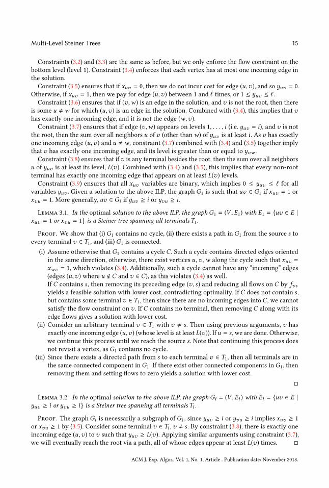
Constraints (3.2) and (3.3) are the same as before, but we only enforce the flow constraint on the

bottom level (level 1). Constraint (3.4) enforces that each vertex has at most one incoming edge in

the solution.

Constraint (3.5) ensures that if xuv = 0, then we do not incur cost for edge (u,v), and so yuv = 0.

Otherwise, if xuv = 1, then we pay for edge (u,v) between 1 and ℓ times, or 1 ≤ yuv ≤ ℓ.Constraint (3.6) ensures that if (v,w) is an edge in the solution, and v is not the root, then there

is some u , w for which (u,v) is an edge in the solution. Combined with (3.4), this implies that vhas exactly one incoming edge, and it is not the edge (w,v).Constraint (3.7) ensures that if edge (v,w) appears on levels 1, . . . , i (i.e. yuv = i), and v is not

the root, then the sum over all neighbors u of v (other thanw) of yuv is at least i . As v has exactly

one incoming edge (u,v) and u , w , constraint (3.7) combined with (3.4) and (3.5) together imply

that v has exactly one incoming edge, and its level is greater than or equal to yvw .Constraint (3.8) ensures that ifv is any terminal besides the root, then the sum over all neighbors

u of yuv is at least its level, L(v). Combined with (3.4) and (3.5), this implies that every non-root

terminal has exactly one incoming edge that appears on at least L(v) levels.Constraint (3.9) ensures that all xuv variables are binary, which implies 0 ≤ yuv ≤ ℓ for all

variables yuv . Given a solution to the above ILP, the graph G1 is such that uv ∈ G1 if xuv = 1 or

xvu = 1. More generally, uv ∈ Gi if yuv ≥ i or yvu ≥ i .

Lemma 3.1. In the optimal solution to the above ILP, the graph G1 = (V ,E1) with E1 = {uv ∈ E |xuv = 1 or xvu = 1} is a Steiner tree spanning all terminals T1.

Proof. We show that (i)G1 contains no cycle, (ii) there exists a path in G1 from the source s toevery terminal v ∈ T1, and (iii) G1 is connected.

(i) Assume otherwise that G1 contains a cycle C . Such a cycle contains directed edges oriented

in the same direction, otherwise, there exist vertices u, v ,w along the cycle such that xuv =xwv = 1, which violates (3.4). Additionally, such a cycle cannot have any “incoming” edges

(edges (u,v) where u < C and v ∈ C), as this violates (3.4) as well.If C contains s , then removing its preceding edge (v, s) and reducing all flows on C by fvsyields a feasible solution with lower cost, contradicting optimality. If C does not contain s ,but contains some terminal v ∈ T1, then since there are no incoming edges intoC , we cannotsatisfy the flow constraint on v . If C contains no terminal, then removing C along with its

edge flows gives a solution with lower cost.

(ii) Consider an arbitrary terminal v ∈ T1 with v , s . Then using previous arguments, v has

exactly one incoming edge (u,v) (whose level is at least L(v)). Ifu = s , we are done. Otherwise,we continue this process until we reach the source s . Note that continuing this process does

not revisit a vertex, as G1 contains no cycle.

(iii) Since there exists a directed path from s to each terminal v ∈ T1, then all terminals are in

the same connected component in G1. If there exist other connected components in G1, then

removing them and setting flows to zero yields a solution with lower cost.

□

Lemma 3.2. In the optimal solution to the above ILP, the graph Gi = (V ,Ei ) with Ei = {uv ∈ E |yuv ≥ i or yvu ≥ i} is a Steiner tree spanning all terminals Ti .

Proof. The graphGi is necessarily a subgraph of G1, since yuv ≥ i or yvu ≥ i implies xuv ≥ 1

or xvu ≥ 1 by (3.5). Consider some terminal v ∈ Ti , v , s . By constraint (3.8), there is exactly one

incoming edge (u,v) to v such that yuv ≥ L(v). Applying similar arguments using constraint (3.7),

we will eventually reach the root via a path, all of whose edges appear at least L(v) times. □


16 R. Ahmed et al.

Theorem 3.3. The optimal solution to the above ILP with cost OPTI LP yields the optimal MLSTsolution.

Proof. The optimal MLST solution whose cost is OPT is a feasible solution to the ILP, as we

can set the xuv , yuv , and fuv variables accordingly, so OPTI LP ≤ OPT. By Lemmas 3.1 and 3.2, the

optimal solution OPTI LP gives a feasible solution to the MLST problem, so OPT ≤ OPTI LP . Then

OPT = OPTI LP . □

The number of flow variables is 2|E | (where |E | is the number of edges in the input graph), and

the total number of variables is O(|E |). The number of flow constraints is O(|V |) and the total

number of constraints isO(|V | + |E |). Additionally, the integrality constraints on the flow variables

fuv as well as the variables yuv may be dropped without affecting the optimal solution.

4 EXPERIMENTAL RESULTS

Graph Data Synthesis. The graphs we used in our experiment are synthesized from graph

generation models. In particular, we used three random network generation models: Erdős–Renyi

(ER) [9], Watts–Strogatz (WS) [20], and Barabási–Albert (BA) [3]. These networks are very well

studied in the literature [16].

The Erdős–Renyi model, ER(n,p), assigns an edge to every possible pair among n = |V | verticeswith probability p, independently of other edges. It is well-known that an instance of ER(n,p) withp = (1+ε) lnnn is almost surely connected for ε > 0 [9]. For our experiment, n = 50, 100, 150, . . . , 500,and ε = 1.

The Watts–Strogatz model, WS(n,K , β), initially creates a ring lattice of constant degree K , andthen rewires each edge with probability 0 ≤ β ≤ 1 while avoiding self-loops or duplicate edges.

Interestingly, the Watts–Strogatz model generates graphs that have the small-world property while

having high clustering coefficient [20]. In our experiment, the values of K and β are equal to 6 and

0.2 respectively.The Barabási–Albert model, BA(m0,m), uses a preferential attachment mechanism to generate a

growing scale-free network. The model starts with a graph ofm0 vertices. Then, each new vertex

connects tom ≤ m0 existing nodes with probability proportional to its instantaneous degree. The

BA model generates networks with power-law degree distribution, i.e. few vertices become hubs

with extremely large degree [3]. This model is a network growth model. In our experiments, we

let the network grow until a desired network size n is attained. We varym0 from 10 to 100 in our

experiments. We keep the value ofm equal to 5.

For each generation model, we generate graphs on size |V | = 50, 100, 150, . . . , 500. On each graph

instance, we assign integer edge weights c(e) randomly and uniformly between 1 and 10 inclusive.

We only consider connected graphs in our experiment. Computational challenges of solving an ILP

limit the size of the graphs to a few hundred in practice.

Selection of Levels and Terminals. For each generated graph, we generated MLST instances

with ℓ = 2, 3, 4, 5 levels. We adopted two strategies for selecting the terminals on the ℓ levels: linearvs. exponential. In the linear case, we select the terminals on each level by randomly sampling

⌊|V | · (ℓ − i + 1)/(ℓ + 1)⌋ vertices on level i so that the size of the terminal sets decreases linearly.

As the terminal sets are nested, Ti can be selected by sampling from Ti−1 (or from V if i = 1). In the

exponential case, we select the terminals on each level by randomly sampling ⌊|V |/2ℓ−i+1⌋ verticesso that the size of the terminal sets decreases exponentially by a factor of 2.

To summarize, a single instance of an input to the MLST problem is characterized by four

parameters: network generation model NGM ∈ {ER,WS,BA}, number of vertices |V |, number of

levels ℓ, and the terminal selection method TSM ∈ {Linear,Exponential}. Since each instance of



the experiment setup involves randomness at different steps, we generated 5 instances for every

choice of parameters (e.g., WS, |V | = 100, ℓ = 5, Linear).

Algorithms and Outputs.We implemented the bottom-up, top-down, and composite heuristics

described in Section 2.

For evaluating the heuristics, we also implemented all ILPs described in Section 3 using CPLEX

12.6.2 as an ILP solver. The ILP described in Section 3.4 works very well in practice. Hence, we

have used this ILP for our experiment. The model of the HPC system we used for our experiment

is Lenovo NeXtScale nx360 M5. It is a distributed system; the models of the processors in this HPC

are Xeon Haswell E5-2695 Dual 14-core and Xeon Broadwell E5-2695 Dual 14-core. The speed of a

processor is 2.3 GHz. There are 400 nodes each having 28 cores. Each node has 192 GB memory.

The operating system is CentOS 6.10.

For each instance of the MLST problem, we compute the costs of the MLST from the ILP solution

(OPT), the bottom-up solution (BOT), the top-down solution (TOP), the composite heuristic (CMP),

and the guaranteed performance heuristic (CMP(Q∗) where Q∗is chosen suitably). The four

heuristics involve a (single-level) ST subroutine; we used both the 2-approximation algorithm of

Gilbert and Pollak [10], as well as the flow formulation described in Section 3.4 which solves ST

optimally. The purpose of this is to assess whether solving ST optimally significantly improves the

approximation ratio.

After completing the experiment, we compared the results of the heuristics with exact solutions.

We show the performance ratio for each heuristic (defined as the heuristic cost divided byOPT), and

how the ratio depends on the experiment parameters (number of levels ℓ, terminal selection method,

number of vertices |V |). We record the number of ST computations involved for the guaranteed

performance heuristic (CMP(Q∗)) (note that this equals ℓ + |Q∗ |). Finally, we discuss the runningtime of the ILP we have used in our experiment. All box plots shown below show the minimum,

interquartile range (IQR) and maximum, aggregated over all instances using the parameter being

compared.

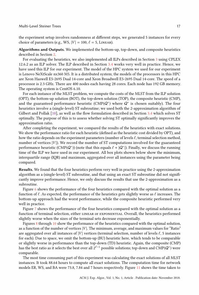
Results.We found that the four heuristics perform very well in practice using the 2-approximation

algorithm as a (single-level) ST subroutine, and that using an exact ST subroutine did not signifi-

cantly improve performance. Hence, we only discuss the results that use the 2-approximation as a

subroutine.

Figure 6 shows the performance of the four heuristics compared with the optimal solution as a

function of ℓ. As expected, the performance of the heuristics gets slightly worse as ℓ increases. Thebottom-up approach had the worst performance, while the composite heuristic performed very

well in practice.

Figure 7 shows the performance of the four heuristics compared with the optimal solution as a

function of terminal selection, either linear or exponential. Overall, the heuristics performed

slightly worse when the sizes of the terminal sets decrease exponentially.

Figures 8 through 10 show the performance of the heuristics compared with the optimal solution,

as a function of the number of vertices |V |. The minimum, average, and maximum values for “Ratio”

are aggregated over all instances of |V | vertices (terminal selection, number of levels ℓ, 5 instancesfor each). Due to space, we omit the bottom-up (BU) heuristic here, which tends to be comparable

or slightly worse in performance than the top-down (TD) heuristic. Again, the composite (CMP)

has the best ratio as it selects the best over all 2ℓ−1

possible solutions; top-down and CMP(Q∗) werecomparable.

The most time consuming part of this experiment was calculating the exact solutions of all MLST

instances. It took 88.64 hours to compute all exact solutions. The computation time for network

models ER, WS, and BA were 73.8, 7.84 and 7 hours respectively. Figure 11 shows the time taken to


18 R. Ahmed et al.

(a) Barabási–Albert (b) Erdős–Rényi (c) Watts–Strogatz

Fig. 6. Performance of BOT, TOP, CMP, and CMP(Q∗) w.r.t. the number ℓ of levels using the 2-approximation

for ST as a subroutine.


Fig. 7. Performance of BOT, TOP, CMP, and CMP(Q∗) w.r.t. the terminal selection method using the 2-

approximation for ST as a subroutine.

compute the exact solutions (with cost OPT), as a function of the number of levels ℓ. As expected,the running time of the heuristics gets worse as ℓ increases. Note that the y-axes of the graphs inthese figures have different scales for different network models. The Erdős–Rényi network model

had the highest running time in the worst case.

Figure 12 shows the time taken to compute the exact solutions, as a function of the terminal

selection method, either linear or exponential. Overall, the running times are slightly worse

when the size of the terminal sets decreases exponentially, especially in the worst case.

Figure 13 shows the time taken to compute the exact solutions, for each of the network models

BA, ER, WS, as a function of the number of vertices |V |. Since several instances share the same

network size, we show minimum, mean, and maximum values. Note that the y-axes of the graphsin these figures have different scales for different network models. As expected, the running time

slightly deteriorated as |V | increased, especially in the worst case.

5 CONCLUSIONSWe presented several heuristics for the MLST problem and analyzed them both theoretically and

experimentally. All the software (new heusritcs, approximation algorithms, ILP solvers, experimen-

tal data and analysis) are available online https://github.com/abureyanahmed/multi_level_steiner_

trees.

The heuristics in this article rely on single level ST subroutines. The composite heuristic CMP

achieves the best approximation ratio, as it is the minimum of all possible combinations of single


https://github.com/abureyanahmed/multi_level_steiner_ trees



(a) Top-down (b) Composite (c) CMP(Q∗)

Fig. 8. Performance of TOP, CMP, and CMP(Q∗) on Erdős–Rényi graphs using the 2-approximation for ST as

a subroutine.


Fig. 9. Performance of TOP, CMP, and CMP(Q∗) on Watts–Strogatz graphs.


Fig. 10. Performance of TOP, CMP, and CMP(Q∗) on Barabási–Albert graphs using the 2-approximation for

ST as a subroutine.

level ST computations. Importantly, we showed that CMP(Q∗) guarantees the same approximation

ratio that CMP can provide, using at most 2ℓ ST computations, rather thanO(2ℓ−1ℓ). One important

question is to consider whether it is possible to directly approximate the MLST problem, without

the use of multiple single level ST subroutines, and whether it is possible to do better than the CMP

approximation ratio. Further, it is natural to study whether there are stronger inapproximability

results for the MLST problem, compared to the standard ST problem.

Another interesting open problem is whether the approximation ratios tℓ (Section 2.2) are tight

for any ℓ, and whether the output y from the LP formulation can help in designing worst-case


20 R. Ahmed et al.


Fig. 11. Experimental running times for computing exact solutions w.r.t. the number ℓ of levels, aggregated

over all instances with ℓ levels.


Fig. 12. Experimental running times for computing exact solutions w.r.t. the terminal selection method,

aggregated over all instances with Linear or Exponential terminal selection.


Fig. 13. Experimental running times for computing exact solutions w.r.t. the graph size |V |, aggregated over

all instances of |V | vertices.

examples. In particular, even though we have computed the approximation ratio for up to ℓ = 100

levels, it remains to determine the limit limℓ→∞ tℓ .As a final remark, even though our investigation was only focused on the MLST problem, much

of the analysis does not depend on the fact that we computed Steiner trees, but only that the

computed graphs were nested. We thus wonder whether it is possible to generalize our results to

other “sparsifiers” (e.g., node-weighted Steiner trees, graph t-spanners).



REFERENCES[1] Sanjeev Arora. 1998. Polynomial Time Approximation Schemes for Euclidean Traveling Salesman and other Geometric

Problems. J. ACM 45, 5 (1998), 753–782. https://doi.org/10.1145/290179.290180

[2] Anantaram Balakrishnan, Thomas L. Magnanti, and Prakash Mirchandani. 1994. Modeling and Heuristic Worst-

Case Performance Analysis of the Two-Level Network Design Problem. Management Sci. 40, 7 (1994), 846–867.

https://doi.org/10.1287/mnsc.40.7.846

[3] Albert-László Barabási and Réka Albert. 1999. Emergence of scaling in random networks. science 286, 5439 (1999),509–512.

[4] Marshall Bern and Paul Plassmann. 1989. The Steiner problem with edge lengths 1 and 2. Inform. Process. Lett. 32, 4(1989), 171–176. https://doi.org/10.1016/0020-0190(89)90039-2

[5] Jaroslaw Byrka, Fabrizio Grandoni, Thomas Rothvoß, and Laura Sanità. 2013. Steiner Tree Approximation via Iterative

Randomized Rounding. J. ACM 60, 1 (2013), 6:1–6:33. https://doi.org/10.1145/2432622.2432628

[6] Moses Charikar, Joseph (Seffi) Naor, and Baruch Schieber. 2004. Resource optimization in QoS multicast routing of

real-time multimedia. IEEE/ACM Trans. Networking 12, 2 (2004), 340–348. https://doi.org/10.1109/TNET.2004.826288

[7] Miroslav Chlebík and Janka Chlebíková. 2008. The Steiner tree problem on graphs: Inapproximability results. Theoret.Comput. Sci. 406, 3 (2008), 207–214. https://doi.org/10.1016/j.tcs.2008.06.046

[8] Julia Chuzhoy, Anupam Gupta, Joseph (Seffi) Naor, and Amitabh Sinha. 2008. On the Approximability of Some Network

Design Problems. ACM Trans. Algorithms 4, 2 (2008), 23:1–23:17. https://doi.org/10.1145/1361192.1361200

[9] Paul Erdös and Alfréd Rényi. 1959. On Random Graphs I. Publicationes Mathematicae (Debrecen) 6 (1959), 290–297.[10] Edgar N. Gilbert and Henry O. Pollak. 1968. Steiner Minimal Trees. SIAM J. Appl. Math. 16, 1 (1968), 1–29. https:

//doi.org/10.1137/0116001

[11] Mathias Hauptmann and Marek Karpinski (eds.). 2015. A Compendium on Steiner Tree Problems. http://theory.cs.

uni-bonn.de/info5/steinerkompendium/

[12] Richard M. Karp. 1972. Reducibility among Combinatorial Problems. In Complexity of Computer Computations,Raymond E. Miller, James W. Thatcher, and Jean D. Bohlinger (Eds.). Plenum Press, 85–103. https://doi.org/10.1007/

978-1-4684-2001-2_9

[13] Marek Karpinski, Ion I. Mandoiu, Alexander Olshevsky, and Alexander Zelikovsky. 2005. Improved Approximation

Algorithms for the Quality of Service Multicast Tree Problem. Algorithmica 42, 2 (2005), 109–120. https://doi.org/10.

1007/s00453-004-1133-y

[14] Prakash Mirchandani. 1996. The multi-tier tree problem. INFORMS J. Comput. 8, 3 (1996), 202–218.[15] Joseph S. B. Mitchell. 1999. Guillotine Subdivisions Approximate Polygonal Subdivisions: A Simple Polynomial-Time

Approximation Scheme for Geometric TSP, k-MST, and Related Problems. SIAM J. Comput. 28, 4 (1999), 1298–1309.https://doi.org/10.1137/S0097539796309764

[16] Mark E.J. Newman. 2003. The structure and function of complex networks. SIAM Rev. 45, 2 (2003), 167–256. https:

//doi.org/10.1137/S003614450342480

[17] Tobias Polzin and Siavash Vahdati Daneshmand. 2001. A comparison of Steiner tree relaxations. Discrete Appl. Math.112, 1 (2001), 241–261. https://doi.org/10.1016/S0166-218X(00)00318-8

[18] Hans Jürgen Prömel and Angelika Steger. 2002. The Steiner Tree Problem. Vieweg and Teubner Verlag.

[19] Gabriel Robins and Alexander Zelikovsky. 2005. Tighter Bounds for Graph Steiner Tree Approximation. SIAM J.Discrete Math. 19, 1 (2005), 122–134. https://doi.org/10.1137/S0895480101393155

[20] Duncan J. Watts and Steven H. Strogatz. 1998. Collective dynamics of ’small-world’ networks. Nature 393, 6684 (1998),440–442. https://doi.org/10.1038/30918

[21] Pawel Winter. 1987. Steiner Problem in Networks: A Survey. Networks 17, 2 (1987), 129–167. https://doi.org/10.1002/

net.3230170203

[22] Guoliang Xue, Guo-Hui Lin, and Ding-Zhu Du. 2001. Grade of Service Steiner Minimum Trees in the Euclidean Plane.

Algorithmica 31, 4 (2001), 479–500. https://doi.org/10.1007/s00453-001-0050-6


https://doi.org/10.1145/290179.290180

https://doi.org/10.1287/mnsc.40.7.846

https://doi.org/10.1016/0020-0190(89)90039-2

https://doi.org/10.1145/2432622.2432628

https://doi.org/10.1109/TNET.2004.826288

https://doi.org/10.1016/j.tcs.2008.06.046

https://doi.org/10.1145/1361192.1361200

https://doi.org/10.1137/0116001

https://doi.org/10.1137/0116001

http://theory.cs.uni-bonn.de/info5/steinerkompendium/

http://theory.cs.uni-bonn.de/info5/steinerkompendium/

https://doi.org/10.1007/978-1-4684-2001-2_9

https://doi.org/10.1007/978-1-4684-2001-2_9

https://doi.org/10.1007/s00453-004-1133-y

https://doi.org/10.1007/s00453-004-1133-y

https://doi.org/10.1137/S0097539796309764

https://doi.org/10.1137/S003614450342480

https://doi.org/10.1137/S003614450342480

https://doi.org/10.1016/S0166-218X(00)00318-8

https://doi.org/10.1137/S0895480101393155

https://doi.org/10.1038/30918

https://doi.org/10.1002/net.3230170203

https://doi.org/10.1002/net.3230170203

https://doi.org/10.1007/s00453-001-0050-6

22 R. Ahmed et al.

REVISIONS WITH RESPECT TO CONFERENCE VERSION (SEA 2018)We have made the following changes:

• We added the cut-based ILP formulation (Section 3.1), multi-commodity flow based ILP

(section 3.2), as well as a new simplification of the single-commodity ILP (section 3.4) which

reduces the number of variables and constraints by a factor of ℓ. We also added proofs of

correctness for the new ILP formulation.

• The new ILP formulation allowed us to perform experiments with graphs of up to |V | = 500

vertices. Previously we only tested graphs of up to 100 vertices.

• All the software (new heusritcs, approximation algorithms, ILP solvers, experimental data and

analysis) are available online https://github.com/abureyanahmed/multi_level_steiner_trees.

• More thoroughly explained the composite heuristic (Section 2.2), added Lemma 2.3, and

provided a better treatment of Theorem 2.5 with additional discussion.

• Derived how to compute an approximation ratio for CMP(Q) for any Q ⊆ {1, 2, . . . , ℓ} insection 2.2. This yields an alternate proof of the

ℓ+12, ℓ, and 4-approximations for top-down,

bottom-up, and the QoS algorithms.

• Found an approximation ratio for CMP using column-generation techniques that allows us

to compute the exact approximation ratio in Figure 5 up to ℓ = 100, which is much larger

than any practical need. Previously, we were only able to compute values up to ℓ = 22 levels.

• Included experimental running times for computing OPT in Figures 11, 12, 13. These show

min, average, and max running times depending on number of levels ℓ, terminal selection

method, and number of vertices |V |.• Experimentedwith the use of an exact Steiner tree subroutine and the use of the 2-approximation

algorithm in the proposed algorithms. We found that the four algorithms perform very well

in practice with the 2-approximation algorithm as a (single-level) ST subroutine, and that

using an exact ST subroutine does not noticeably improve the performance. Hence, we only

discuss the results that use the 2-approximation algorithm.

• We expanded and improved the Conclusions section, discussing several open problems.

• We changed the notation for the number of levels from k to ℓ and renumber them 1, . . . , ℓwith level ℓ on top (previously k , . . . , 1 with 1 on top). This is more intuitive as it clearly

indicates that an edge on level i (but not i + 1) pays i times its cost (rather than k + 1− i times

as before).

• Clarified and improved several proofs, most notably the TD and BU algorithms, and added

new figures.

Received September 2018



Multi-Level Steiner Trees - arXiv

Documents

Transcript of Multi-Level Steiner Trees - arXiv