A review of deep learning applications for genomic selection

REVIEW Open Access

A review of deep learning applications forgenomic selectionOsval Antonio Montesinos-López1, Abelardo Montesinos-López2*, Paulino Pérez-Rodríguez3,José Alberto Barrón-López4, Johannes W. R. Martini5, Silvia Berenice Fajardo-Flores1, Laura S. Gaytan-Lugo6,Pedro C. Santana-Mancilla1 and José Crossa3,5*

Abstract

Background: Several conventional genomic Bayesian (or no Bayesian) prediction methods have been proposedincluding the standard additive genetic effect model for which the variance components are estimated with mixedmodel equations. In recent years, deep learning (DL) methods have been considered in the context of genomicprediction. The DL methods are nonparametric models providing flexibility to adapt to complicated associationsbetween data and output with the ability to adapt to very complex patterns.

Main body: We review the applications of deep learning (DL) methods in genomic selection (GS) to obtain a meta-picture of GS performance and highlight how these tools can help solve challenging plant breeding problems. Wealso provide general guidance for the effective use of DL methods including the fundamentals of DL and therequirements for its appropriate use. We discuss the pros and cons of this technique compared to traditionalgenomic prediction approaches as well as the current trends in DL applications.

Conclusions: The main requirement for using DL is the quality and sufficiently large training data. Although, basedon current literature GS in plant and animal breeding we did not find clear superiority of DL in terms of predictionpower compared to conventional genome based prediction models. Nevertheless, there are clear evidences that DLalgorithms capture nonlinear patterns more efficiently than conventional genome based. Deep learning algorithmsare able to integrate data from different sources as is usually needed in GS assisted breeding and it shows theability for improving prediction accuracy for large plant breeding data. It is important to apply DL to large training-testing data sets.

Keywords: Genomic selection, Deep learning, Plant breeding, Genomic trends

BackgroundPlant breeding is a key component of strategies aimed atsecuring a stable food supply for the growing humanpopulation, which is projected to reach 9.5 billion peopleby 2050 [1, 2]. To be able to keep pace with the expectedincrease in food demand in the coming years, plant

breeding has to deliver the highest rates of genetic gainto maximize its contribution to increasing agriculturalproductivity. In this context, an essential step is harnes-sing the potential of novel methodologies. Today, gen-omic selection (GS), proposed by Bernardo [3] andMeuwissen et al. [4] has become an established method-ology in breeding. The underlying concept is based onthe use of genome-wide DNA variation (“markers”) to-gether with phenotypic information from an observedpopulation to predict the phenotypic values of an unob-served population. With the decrease in genotyping

© The Author(s). 2021 Open Access This article is licensed under a Creative Commons Attribution 4.0 International License,which permits use, sharing, adaptation, distribution and reproduction in any medium or format, as long as you giveappropriate credit to the original author(s) and the source, provide a link to the Creative Commons licence, and indicate ifchanges were made. The images or other third party material in this article are included in the article's Creative Commonslicence, unless indicated otherwise in a credit line to the material. If material is not included in the article's Creative Commonslicence and your intended use is not permitted by statutory regulation or exceeds the permitted use, you will need to obtainpermission directly from the copyright holder. To view a copy of this licence, visit http://creativecommons.org/licenses/by/4.0/.The Creative Commons Public Domain Dedication waiver (http://creativecommons.org/publicdomain/zero/1.0/) applies to thedata made available in this article, unless otherwise stated in a credit line to the data.

* Correspondence: [email protected]; [email protected] de Matemáticas, Centro Universitario de Ciencias Exactas eIngenierías (CUCEI), Universidad de Guadalajara, 44430 Guadalajara, Jalisco,Mexico3Colegio de Postgraduados, CP 56230 Montecillos, Edo. de México, MexicoFull list of author information is available at the end of the article

Montesinos-López et al. BMC Genomics (2021) 22:19 https://doi.org/10.1186/s12864-020-07319-x

http://crossmark.crossref.org/dialog/?doi=10.1186/s12864-020-07319-x&domain=pdf

http://orcid.org/0000-0001-9429-5855

http://creativecommons.org/licenses/by/4.0/

http://creativecommons.org/publicdomain/zero/1.0/

mailto:[email protected]

mailto:[email protected]

costs, GS has become a standard tool in many plant andanimal breeding programs with the main application ofreducing the length of breeding cycles [5–9].Many empirical studies have shown that GS can in-

crease the selection gain per year when used appropri-ately. For example, Vivek et al. [10] compared GS toconventional phenotypic selection (PS) for maize, andfound that the gain per cycle under drought conditionswas 0.27 (t/ha) when using PS, which increased to 0.50(t/ha) when GS was implemented. Divided by the cyclelength, the genetic gain per year under drought condi-tions was 0.067 (PS) compared to 0.124 (GS). Analo-gously, under optimal conditions, the gain increasedfrom 0.34 (PS) to 0.55 (GS) per cycle, which translates to0.084 (PS) and 0.140 (GS) per year. Also for maize,Môro et al. [11] reported a similar selection gain whenusing GS or PS. For soybean [Glycine max (L.) Merr.],Smallwood et al. [12] found that GS outperformed PSfor fatty acid traits, whereas no significant differenceswere found for traits yield, protein and oil. In barley,Salam and Smith [13] reported similar (per cycle) selec-tion gains when using GS or PS, but with the advantagethat GS shortened the breeding cycle and lowered thecosts. GS has also been used for breeding forest tree spe-cies such as eucalyptus, pine, and poplar [14]. Breedingresearch at the International Maize and Wheat Improve-ment Center (CIMMYT) has shown that GS can reducethe breeding cycle by at least half and produce lines withsignificantly increased agronomic performance [15].Moreover, GS has been implemented in breeding pro-grams for legume crops such as pea, chickpea, ground-nut, and pigeon pea [16]. Other studies have consideredthe use of GS for strawberry [17], cassava [18], soybean[19], cacao [20], barley [21], millet [22], carrot [23], ba-nana [24], maize [25], wheat [26], rice [27] and sugarcane [28].Although genomic best linear unbiased prediction

(GBLUP) is in practice the most popular method that isoften equated with genomic prediction, genomic predic-tion can be based on any method that can capture theassociation between the genotypic data and associatedphenotypes (or breeding values) of a training set. By fit-ting the association, the statistical model “learns” howthe genotypic information maps to the quantity that wewould like to predict. Consequently, many genomic pre-diction methods have been proposed. According to VanVleck [29], the standard additive genetic effect model isthe aforementioned GBLUP for which the variance com-ponents have to be estimated and the mixed modelequations of Henderson [30] have to be solved. Alterna-tively, Bayesian methods with different priors using Mar-kov Chain Monte Carlo methods to determine requiredparameters are very popular [31–33]. In recent years,different types of (deep) learning methods have been

considered for their performance in the context of gen-omic prediction. DL is a type of machine learning (ML)approach that is a subfield of artificial intelligence (AI).The main difference between DL methods and conven-tional statistical learning methods is that DL methodsare nonparametric models providing tremendous flexi-bility to adapt to complicated associations between dataand output. A particular strength is the ability to adaptto hidden patterns of unknown structure that thereforecould not be incorporated into a parametric model atthe beginning [34].There is plenty of empirical evidence of the power of

DL as a tool for developing AI systems, products, de-vices, apps, etc. These products are found anywherefrom social sciences to natural sciences, includingtechnological applications in agriculture, finance, medi-cine, computer vision, and natural language processing.Many “high technology” products, such as autonomouscars, robots, chatbots, devices for text-to-speech conver-sion [35, 36], speech recognition systems, digital assis-tants [37] or the strategy of artificial challengers indigital versions of chess, Jeopardy, GO and poker [38],are based on DL. In addition, there are medical applica-tions for identifying and classifying cancer or dermatol-ogy problems, among others. For instance, Menden et al.[39] applied a DL method to predict the viability of acancer cell line exposed to a drug. Alipanahi et al. [40]used DL with a convolutional network architecture topredict specificities of DNA- and RNA-binding proteins.Tavanaei et al. [41] used a DL method for predictingtumor suppressor genes and oncogenes. DL methodshave also made accurate predictions of single-cell DNAmethylation states [42]. In the genomic domain, most ofthe applications concern functional genomics, such aspredicting the sequence specificity of DNA- and RNA-binding proteins, methylation status, gene expression,and control of splicing [43]. DL has been especially suc-cessful when applied to regulatory genomics, by usingarchitectures directly adapted from modern computervision and natural language processing applications.There are also successful applications of DL for high-throughput plant phenotyping [44]; a complete review ofthese applications is provided by Jiang and Li [44].Due to the ever-increasing volume of data in plant

breeding and to the power of DL applications in manyother domains of science, DL techniques have also beenevaluated in terms of prediction performance in GS.Often the results are mixed below the –perhaps exagger-ated– expectations for datasets with relatively smallnumbers of individuals [45]. Here we review DL applica-tions for GS to provide a meta-picture of their potentialin terms of prediction performance compared to con-ventional genomic prediction models. We include anintroduction to DL fundamentals and its requirements

Montesinos-López et al. BMC Genomics (2021) 22:19 of 23

in terms of data size, tuning process, knowledge, type ofinput, computational resources, etc., to apply DL suc-cessfully. We also analyze the pros and cons of this tech-nique compared to conventional genomic predictionmodels, as well as future trends using this technique.

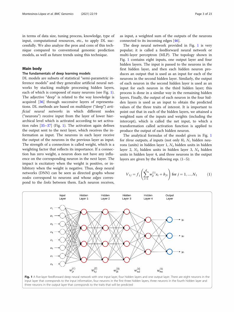
Main bodyThe fundamentals of deep learning modelsDL models are subsets of statistical “semi-parametric in-ference models” and they generalize artificial neural net-works by stacking multiple processing hidden layers,each of which is composed of many neurons (see Fig. 1).The adjective “deep” is related to the way knowledge isacquired [36] through successive layers of representa-tions. DL methods are based on multilayer (“deep”) arti-ficial neural networks in which different nodes(“neurons”) receive input from the layer of lower hier-archical level which is activated according to set activa-tion rules [35–37] (Fig. 1). The activation again definesthe output sent to the next layer, which receives the in-formation as input. The neurons in each layer receivethe output of the neurons in the previous layer as input.The strength of a connection is called weight, which is aweighting factor that reflects its importance. If a connec-tion has zero weight, a neuron does not have any influ-ence on the corresponding neuron in the next layer. Theimpact is excitatory when the weight is positive, or in-hibitory when the weight is negative. Thus, deep neuralnetworks (DNN) can be seen as directed graphs whosenodes correspond to neurons and whose edges corres-pond to the links between them. Each neuron receives,

as input, a weighted sum of the outputs of the neuronsconnected to its incoming edges [46].The deep neural network provided in Fig. 1 is very

popular; it is called a feedforward neural network ormulti-layer perceptron (MLP). The topology shown inFig. 1 contains eight inputs, one output layer and fourhidden layers. The input is passed to the neurons in thefirst hidden layer, and then each hidden neuron pro-duces an output that is used as an input for each of theneurons in the second hidden layer. Similarly, the outputof each neuron in the second hidden layer is used as aninput for each neuron in the third hidden layer; thisprocess is done in a similar way in the remaining hiddenlayers. Finally, the output of each neuron in the four hid-den layers is used as an input to obtain the predictedvalues of the three traits of interest. It is important topoint out that in each of the hidden layers, we attained aweighted sum of the inputs and weights (including theintercept), which is called the net input, to which atransformation called activation function is applied toproduce the output of each hidden neuron.The analytical formulas of the model given in Fig. 1

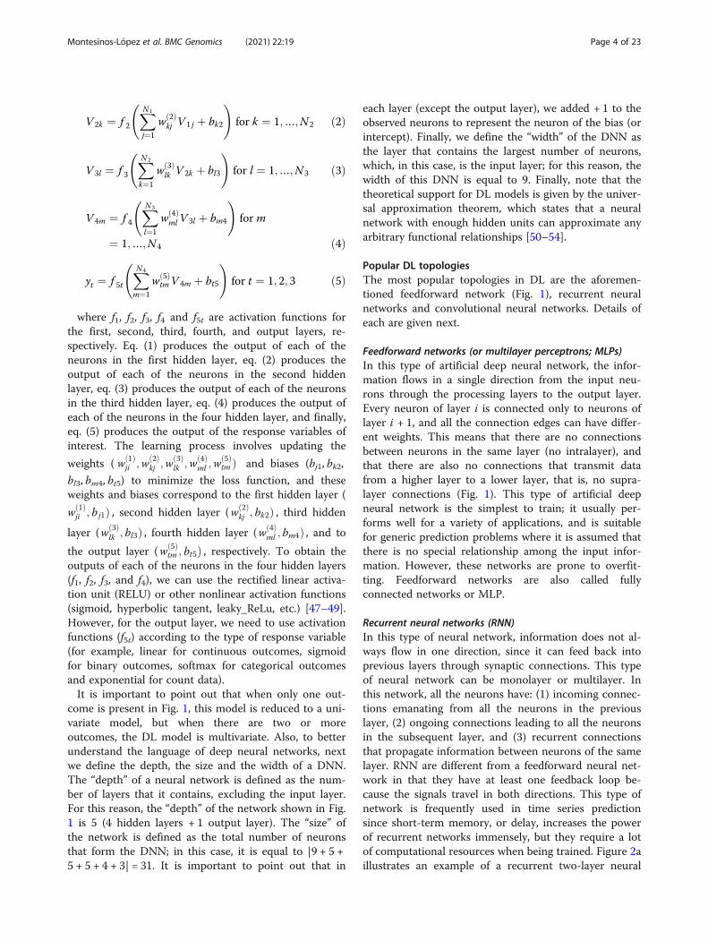
for three outputs, d inputs (not only 8), N1 hidden neu-rons (units) in hidden layer 1, N2 hidden units in hiddenlayer 2, N3 hidden units in hidden layer 3, N4 hiddenunits in hidden layer 4, and three neurons in the outputlayers are given by the following eqs. (1–5):

V 1 j ¼ f 1Xdi¼1

w 1ð Þji xi þ bj1

!for j ¼ 1;…;N1 ð1Þ

Fig. 1 A five-layer feedforward deep neural network with one input layer, four hidden layers and one output layer. There are eight neurons in theinput layer that corresponds to the input information, four neurons in the first three hidden layers, three neurons in the fourth hidden layer andthree neurons in the output layer that corresponds to the traits that will be predicted


V 2k ¼ f 2XN1

j¼1

w 2ð Þkj V 1 j þ bk2

!for k ¼ 1;…;N2 ð2Þ

V 3l ¼ f 3XN2

k¼1

w 3ð Þlk V 2k þ bl3

!for l ¼ 1;…;N3 ð3Þ

V 4m ¼ f 4XN3

l¼1

w 4ð Þml V 3l þ bm4

!for m

¼ 1;…;N4 ð4Þ

yt ¼ f 5tXN4

m¼1

w 5ð ÞtmV 4m þ bt5

!for t ¼ 1; 2; 3 ð5Þ

where f1, f2, f3, f4 and f5t are activation functions forthe first, second, third, fourth, and output layers, re-spectively. Eq. (1) produces the output of each of theneurons in the first hidden layer, eq. (2) produces theoutput of each of the neurons in the second hiddenlayer, eq. (3) produces the output of each of the neuronsin the third hidden layer, eq. (4) produces the output ofeach of the neurons in the four hidden layer, and finally,eq. (5) produces the output of the response variables ofinterest. The learning process involves updating the

weights ( wð1Þji ;wð2Þ

kj ;wð3Þlk ;wð4Þ

ml ;wð5Þtm Þ and biases (bj1, bk2,

bl3, bm4, bt5) to minimize the loss function, and theseweights and biases correspond to the first hidden layer (

wð1Þji ; bj1Þ , second hidden layer (wð2Þ

kj ; bk2Þ , third hidden

layer (wð3Þlk ; bl3Þ , fourth hidden layer (wð4Þ

ml ; bm4Þ , and to

the output layer (wð5Þtm ; bt5Þ , respectively. To obtain the

outputs of each of the neurons in the four hidden layers(f1, f2, f3, and f4), we can use the rectified linear activa-tion unit (RELU) or other nonlinear activation functions(sigmoid, hyperbolic tangent, leaky_ReLu, etc.) [47–49].However, for the output layer, we need to use activationfunctions (f5t) according to the type of response variable(for example, linear for continuous outcomes, sigmoidfor binary outcomes, softmax for categorical outcomesand exponential for count data).It is important to point out that when only one out-

come is present in Fig. 1, this model is reduced to a uni-variate model, but when there are two or moreoutcomes, the DL model is multivariate. Also, to betterunderstand the language of deep neural networks, nextwe define the depth, the size and the width of a DNN.The “depth” of a neural network is defined as the num-ber of layers that it contains, excluding the input layer.For this reason, the “depth” of the network shown in Fig.1 is 5 (4 hidden layers + 1 output layer). The “size” ofthe network is defined as the total number of neuronsthat form the DNN; in this case, it is equal to |9 + 5 +5 + 5 + 4 + 3| = 31. It is important to point out that in

each layer (except the output layer), we added + 1 to theobserved neurons to represent the neuron of the bias (orintercept). Finally, we define the “width” of the DNN asthe layer that contains the largest number of neurons,which, in this case, is the input layer; for this reason, thewidth of this DNN is equal to 9. Finally, note that thetheoretical support for DL models is given by the univer-sal approximation theorem, which states that a neuralnetwork with enough hidden units can approximate anyarbitrary functional relationships [50–54].

Popular DL topologiesThe most popular topologies in DL are the aforemen-tioned feedforward network (Fig. 1), recurrent neuralnetworks and convolutional neural networks. Details ofeach are given next.

Feedforward networks (or multilayer perceptrons; MLPs)In this type of artificial deep neural network, the infor-mation flows in a single direction from the input neu-rons through the processing layers to the output layer.Every neuron of layer i is connected only to neurons oflayer i + 1, and all the connection edges can have differ-ent weights. This means that there are no connectionsbetween neurons in the same layer (no intralayer), andthat there are also no connections that transmit datafrom a higher layer to a lower layer, that is, no supra-layer connections (Fig. 1). This type of artificial deepneural network is the simplest to train; it usually per-forms well for a variety of applications, and is suitablefor generic prediction problems where it is assumed thatthere is no special relationship among the input infor-mation. However, these networks are prone to overfit-ting. Feedforward networks are also called fullyconnected networks or MLP.

Recurrent neural networks (RNN)In this type of neural network, information does not al-ways flow in one direction, since it can feed back intoprevious layers through synaptic connections. This typeof neural network can be monolayer or multilayer. Inthis network, all the neurons have: (1) incoming connec-tions emanating from all the neurons in the previouslayer, (2) ongoing connections leading to all the neuronsin the subsequent layer, and (3) recurrent connectionsthat propagate information between neurons of the samelayer. RNN are different from a feedforward neural net-work in that they have at least one feedback loop be-cause the signals travel in both directions. This type ofnetwork is frequently used in time series predictionsince short-term memory, or delay, increases the powerof recurrent networks immensely, but they require a lotof computational resources when being trained. Figure 2aillustrates an example of a recurrent two-layer neural


network. The output of each neuron is passed through adelay unit and then taken to all the neurons, except it-self. Here, only one input variable is presented to the in-put units, the feedforward flow is computed, and theoutputs are feedback as auxiliary inputs. This leads to adifferent set of hidden unit activations, new output acti-vations, and so on. Ultimately, the activations stabilize,and the final output values are used for predictions.

Convolutional neural networks (CNN)CNN are very powerful tools for performing visual rec-ognition tasks because they are very efficient at captur-ing the spatial and temporal dependencies of the input.CNN use images as input and take advantage of the gridstructure of the data. The efficiency of CNN can be at-tributed in part to the fact that the fitting process re-duces the number of parameters that need to beestimated due to the reduction in the size of the inputand parameter sharing since the input is connected onlyto some neurons. Instead of fully connected layers likethe feedforward networks explained above (Fig. 1), CNNapply convolutional layers which most of the time in-volve the following three operations: convolution, nonlin-ear transformation and pooling. Convolution is a type oflinear mathematical operation that is performed on twomatrices to produce a third one that is usually inter-preted as a filtered version of one of the original matri-ces [48]; the output of this operation is a matrix calledfeature map. The goal of the pooling operation is to pro-gressively reduce the spatial size of the representation toreduce the amount of parameters and computation in

the network. The pooling layer operates on each featuremap independently. The pooling operation performsdown sampling and the most popular pooling operationis max pooling. The max pooling operation summarizesthe input as the maximum within a rectangular neigh-borhood, but does not introduce any new parameters tothe CNN; for this reason, max pooling performs dimen-sional reduction and de-noising. Figure 2b illustrateshow the pooling operation is performed, where we cansee that the original matrix of order 4 × 4 is reduced to adimension of 3 × 3.Figure 3 shows the three stages that conform a convo-

lutional layer in more detail. First, the convolution oper-ation is applied to the input, followed by a nonlineartransformation (like Linear, ReLU, hyperbolic tangent,or another activation function); then the pooling oper-ation is applied. With this convolutional layer, we signifi-cantly reduce the size of the input without relevant lossof information. The convolutional layer picks up differ-ent signals of the image by passing many filters overeach image, which is key for reducing the size of the ori-ginal image (input) without losing critical information,and in early convolutional layers we capture the edges ofthe image. For this reason, CNN include fewer parame-ters to be determined in the learning process, that is, atmost half of the parameters that are needed by a feed-forward deep network (as in Fig. 1). The reduction in pa-rameters has a positive side effect of reducing thetraining times. Also, Fig. 3 indicates that depending onthe complexity of the input (images), the number of con-volutional layers can be more than one to be able to

Fig. 2 A simple two-layer recurrent artificial neural network with univariate outcome (a). Max pooling with 2 × 2 filters and stride 1 (b)


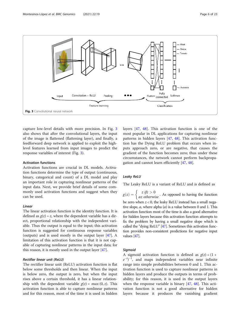
capture low-level details with more precision. In Fig. 3also shows that after the convolutional layers, the inputof the image is flattened (flattening layer), and finally, afeedforward deep network is applied to exploit the high-level features learned from input images to predict theresponse variables of interest (Fig. 3).

Activation functionsActivation functions are crucial in DL models. Activa-tion functions determine the type of output (continuous,binary, categorical and count) of a DL model and playan important role in capturing nonlinear patterns of theinput data. Next, we provide brief details of some com-monly used activation functions and suggest when theycan be used.

LinearThe linear activation function is the identity function. It isdefined as g(z) = z, where the dependent variable has a dir-ect, proportional relationship with the independent vari-able. Thus the output is equal to the input; this activationfunction is suggested for continuous response variables(outputs) and is used mostly in the output layer [47]. Alimitation of this activation function is that it is not cap-able of capturing nonlinear patterns in the input data; forthis reason, it is mostly used in the output layer [47].

Rectifier linear unit (ReLU)The rectifier linear unit (ReLU) activation function is flatbelow some thresholds and then linear. When the inputis below zero, the output is zero, but when the inputrises above a certain threshold, it has a linear relation-ship with the dependent variable g(z) = max (0, z). Thisactivation function is able to capture nonlinear patternsand for this reason, most of the time it is used in hidden

layers [47, 48]. This activation function is one of themost popular in DL applications for capturing nonlinearpatterns in hidden layers [47, 48]. This activation func-tion has the Dying ReLU problem that occurs when in-puts approach zero, or are negative, that causes thegradient of the function becomes zero; thus under thesecircumstances, the network cannot perform backpropa-gation and cannot learn efficiently [47, 48].

Leaky ReLU

The Leaky ReLU is a variant of ReLU and is defined as

gðzÞ ¼ z ifz > 0αz otherwise

�. As opposed to having the function

be zero when z < 0, the leaky ReLU instead has a small nega-tive slope, α, where alpha (α) is a value between 0 and 1. Thisactivation function most of the time is also a good alternativefor hidden layers because this activation function attempts tofix the problem by having a small negative slope which iscalled the “dying ReLU” [47]. Sometimes this activation func-tion provides non-consistent predictions for negative inputvalues [47].

SigmoidA sigmoid activation function is defined as g(z) = (1 +e−z)−1, and maps independent variables near infiniterange into simple probabilities between 0 and 1. This ac-tivation function is used to capture nonlinear patterns inhidden layers and produce the outputs in terms of prob-ability; for this reason, it is used in the output layerswhen the response variable is binary [47, 48]. This acti-vation function is not a good alternative for hiddenlayers because it produces the vanishing gradient

Fig. 3 Convolutional neural network


problem that slows the convergence of the DL model[47, 48].

Softmax

The softmax activation function defined as gðz jÞ

¼ expðz jÞ1þPC

c¼1expðzcÞ

, j = 1,..,C, is a generalization of the sigmoid

activation function that handles multinomial labeling sys-tem; that is, it is appropriate for categorical outcomes. Italso has the property that the sum of the probabilities ofall the categories is equal to one. Softmax is the functionyou will often find in the output layer of a classifier withmore than two categories [47, 48]. This activation functionis recommended only in the output layer [47, 48].

TanhThe hyperbolic tangent (Tanh) activation function is de-

fined as tanhðzÞ ¼ sinhðzÞ= coshðzÞ ¼ expðzÞ − expð − zÞexpðzÞþ expð − zÞ .

Like the sigmoid activation function, the hyperbolic tan-gent has a sigmoidal (“S” shaped) output, with the ad-vantage that it is less likely to get “stuck” than thesigmoid activation function since its output values arebetween − 1 and 1. For this reason, this activation func-tion is recommended for hidden layers and output layersfor predicting response variables in the interval between− 1 and 1 [47, 48]. The vanishing gradient problem issometimes present in this activation function, but it isless common and problematic than when the sigmoidactivation function is used in hidden layers [47, 48].

ExponentialThis activation function handles count outcomes be-cause it guarantees positive outcomes. Exponential is thefunction often used in the output layer for the predictionof count data. The exponential activation function is de-fined as g(z) = exp (z).

Tuning hyper-parametersFor training DL models, we need to distinguish betweenlearnable (structure) parameters and non-learnable(hyper-parameters) parameters. Learnable parametersare learned by the DL algorithm during the trainingprocess (like weights and bias), while hyper-parametersare set before the user begins the learning process,which means that hyper-parameters (like number ofneurons in hidden layers, number of hidden layers, typeof activation function, etc.) are not learned by the DL(or machine learning) method. Hyper-parameters governmany aspects of the behavior of DL models, since differ-ent hyper-parameters often result in significantly differ-ent performance. However, a good choice of hyper-parameters is challenging; for this reason, most of the

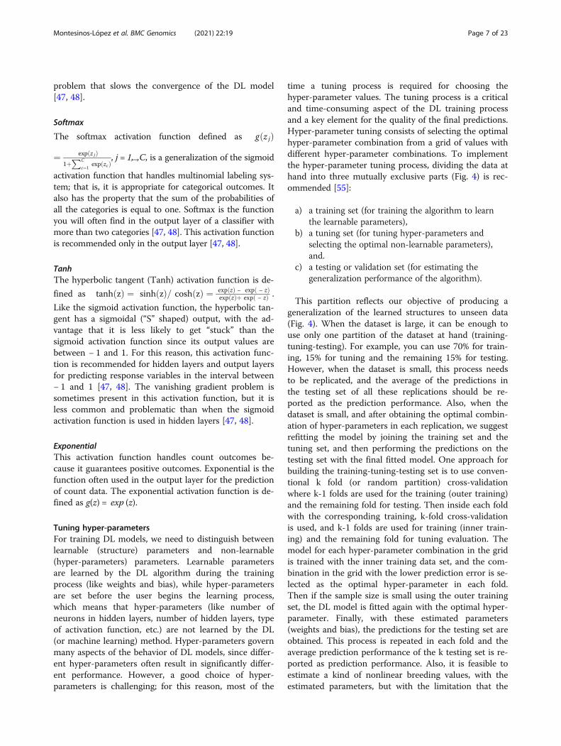
time a tuning process is required for choosing thehyper-parameter values. The tuning process is a criticaland time-consuming aspect of the DL training processand a key element for the quality of the final predictions.Hyper-parameter tuning consists of selecting the optimalhyper-parameter combination from a grid of values withdifferent hyper-parameter combinations. To implementthe hyper-parameter tuning process, dividing the data athand into three mutually exclusive parts (Fig. 4) is rec-ommended [55]:

a) a training set (for training the algorithm to learnthe learnable parameters),

b) a tuning set (for tuning hyper-parameters andselecting the optimal non-learnable parameters),and.

c) a testing or validation set (for estimating thegeneralization performance of the algorithm).

This partition reflects our objective of producing ageneralization of the learned structures to unseen data(Fig. 4). When the dataset is large, it can be enough touse only one partition of the dataset at hand (training-tuning-testing). For example, you can use 70% for train-ing, 15% for tuning and the remaining 15% for testing.However, when the dataset is small, this process needsto be replicated, and the average of the predictions inthe testing set of all these replications should be re-ported as the prediction performance. Also, when thedataset is small, and after obtaining the optimal combin-ation of hyper-parameters in each replication, we suggestrefitting the model by joining the training set and thetuning set, and then performing the predictions on thetesting set with the final fitted model. One approach forbuilding the training-tuning-testing set is to use conven-tional k fold (or random partition) cross-validationwhere k-1 folds are used for the training (outer training)and the remaining fold for testing. Then inside each foldwith the corresponding training, k-fold cross-validationis used, and k-1 folds are used for training (inner train-ing) and the remaining fold for tuning evaluation. Themodel for each hyper-parameter combination in the gridis trained with the inner training data set, and the com-bination in the grid with the lower prediction error is se-lected as the optimal hyper-parameter in each fold.Then if the sample size is small using the outer trainingset, the DL model is fitted again with the optimal hyper-parameter. Finally, with these estimated parameters(weights and bias), the predictions for the testing set areobtained. This process is repeated in each fold and theaverage prediction performance of the k testing set is re-ported as prediction performance. Also, it is feasible toestimate a kind of nonlinear breeding values, with theestimated parameters, but with the limitation that the


estimated parameters in general are not interpretable asin linear regression models.

DL frameworksDL with univariate or multivariate outcomes can be imple-mented in the Keras library as front-end and Tensorflow asback-end [48] in a very user-friendly way. Another popularframework for DL is MXNet, which is efficient and flexibleand allows mixing symbolic programming and imperativeprogramming to maximize efficiency and productivity [56].Efficient DL implementations can also be performed inPyTorch [57] and Chainer [58], but these frameworks arebetter for advanced implementations. Keras in R or Pythonare friendly frameworks that can be used by plant breedersfor implementing DL; however, although they are consid-ered high-level frameworks, the user still needs to have abasic understanding of the fundamentals of DL models tobe able to do successful implementations. Since the userneeds to specify the type of activation functions for thelayers (hidden and output), the appropriate loss function,and the appropriate metrics to evaluate the validation set,the number of hidden layers needs to be added manuallyby the user; he/she also has to choose the appropriate set ofhyper-parameters for the tuning process.Thanks to the availability of more frameworks for imple-

menting DL algorithms, the democratization of this tool willcontinue in the coming years since every day there are moreuser-friendly and open-source frameworks that, in a moreautomatic way and with only some lines of code, allow thestraightforward implementation of sophisticated DL modelsin any domain of science. This trend is really nice, since inthis way, this powerful tool can be used by any professionalwithout a strong background in computer science or math-ematics. Finally, since our goal is not to provide an exhaustivereview of DL frameworks, those interested in learning moredetails about DL frameworks should read [47, 48, 59, 60].

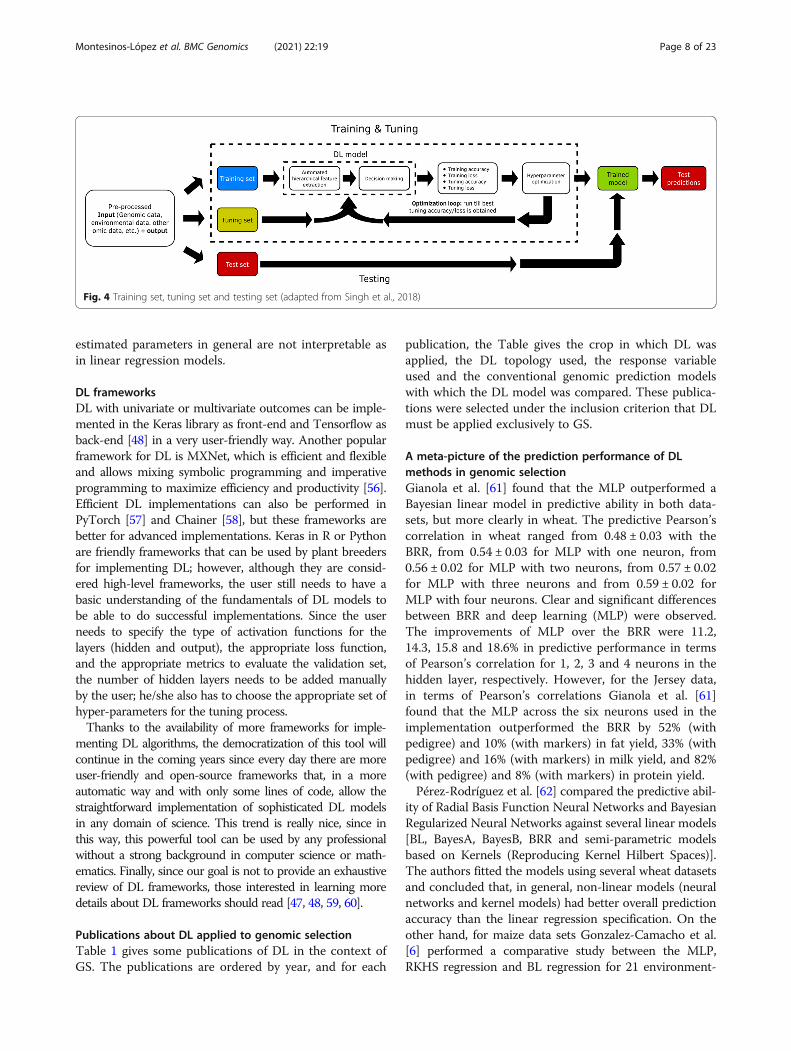
Publications about DL applied to genomic selectionTable 1 gives some publications of DL in the context ofGS. The publications are ordered by year, and for each

publication, the Table gives the crop in which DL wasapplied, the DL topology used, the response variableused and the conventional genomic prediction modelswith which the DL model was compared. These publica-tions were selected under the inclusion criterion that DLmust be applied exclusively to GS.

A meta-picture of the prediction performance of DLmethods in genomic selectionGianola et al. [61] found that the MLP outperformed aBayesian linear model in predictive ability in both data-sets, but more clearly in wheat. The predictive Pearson’scorrelation in wheat ranged from 0.48 ± 0.03 with theBRR, from 0.54 ± 0.03 for MLP with one neuron, from0.56 ± 0.02 for MLP with two neurons, from 0.57 ± 0.02for MLP with three neurons and from 0.59 ± 0.02 forMLP with four neurons. Clear and significant differencesbetween BRR and deep learning (MLP) were observed.The improvements of MLP over the BRR were 11.2,14.3, 15.8 and 18.6% in predictive performance in termsof Pearson’s correlation for 1, 2, 3 and 4 neurons in thehidden layer, respectively. However, for the Jersey data,in terms of Pearson’s correlations Gianola et al. [61]found that the MLP across the six neurons used in theimplementation outperformed the BRR by 52% (withpedigree) and 10% (with markers) in fat yield, 33% (withpedigree) and 16% (with markers) in milk yield, and 82%(with pedigree) and 8% (with markers) in protein yield.Pérez-Rodríguez et al. [62] compared the predictive abil-

ity of Radial Basis Function Neural Networks and BayesianRegularized Neural Networks against several linear models[BL, BayesA, BayesB, BRR and semi-parametric modelsbased on Kernels (Reproducing Kernel Hilbert Spaces)].The authors fitted the models using several wheat datasetsand concluded that, in general, non-linear models (neuralnetworks and kernel models) had better overall predictionaccuracy than the linear regression specification. On theother hand, for maize data sets Gonzalez-Camacho et al.[6] performed a comparative study between the MLP,RKHS regression and BL regression for 21 environment-

Fig. 4 Training set, tuning set and testing set (adapted from Singh et al., 2018)


Table 1 DL application to genomic selectionObs Year Authors Crop Topology Response variable(s) Comparison with

1 2011 Gianola et al.[61]

Wheat and Jerseycows

MLP Grain yield (GY), fat yield, milk yield, protein yield, fat yield Bayesian Ridge regression (BRR)

2 2012 Pérez-Rodríguezet al. [62]

Wheat MLP GY and days to heading (DTHD) BL, BayesA, BayesB, BRR, ReproducingKernel Hilbert Spaces (RKHS)regression

3 2012 Gonzalez-Camachoet al. [6]

Maize MLP GY, female flowering (FFL) or days to silking, male floweringtime (MFL) or days to anthesis, and anthesis-silking interval(ASI)

RKHS regression, BL

4 2015 Ehret et al.[63]

Holstein-Friesian andGerman Fleckvihcattle

MLP Milk yield, protein yield, and fat yield GBLUP

5 2016 Gonzalez-Camachoet al. [64]

Maize and wheat MLP GY Probabilistic neural network (PNN)

6 2016 McDowell [65] Arabidopsis, maizeand wheat

MLP Days to flowering, dry matter, grain yield (GY), spike grain, timeto young microspore.

OLS, RR, LR, ER, BRR

7 2017 Rachmatiaet al. [66]

Maize DBN GY, female flowering (FFL) (or days to silking), male flowering(MFL) (or days to anthesis), and the anthesis-silking interval(ASI)

RKHS, BL and GBLUP

8 2018 Ma et al. [67] Wheat CNN andMLP

Grain length (GL), grain width (GW), thousand-kernel weight(TW), grain protein (GP), and plant height (PH)

RR-BLUP, GBLUP

9 2018 Waldmann[68]

Pig data and TLMAS2010 data

MLP Trait number of live born piglets GBLUP, BL

10 2018 Montesinos-López et al.[70]

Maize and wheat MLP Grain yield GBLUP


Maize and wheat MLP Grain yield (GY), anthesis-silking interval (ASI), PH, days to head-ing (DTHD), days to maturity (DTMT)

BMTME

12 2018 Bellot et al.[72]

Human traits MLP andCNN

Height and bone heel mineral density BayesB, BRR


Wheat MLP GY, DTHD, DTMT, PH, lodging, grain color (GC), leaf rust andstripe rust

SVM, TGBLUP


Wheat MLP GY, DH, PH GBLUP

15 2019 Khaki andWang [75]

Maize MLP GY, check yield, yield difference LR, regression tree

16 2019 Azodi et al.[77]

6 species MLP 18 traits rrBLUP, BRR, BA, BB, BL, SVM, GTB

17 2019 Liu et al. [78] Soybean CNN GY, protein, oil, moisture, PH rrBLUP, BRR, BayesA, BL

18 2020 Abdollahi-Arpanahi et al.[79]

Holstein bulls MLP andCNN

Sire conception rate GBLUP, BayesB and RF

19 2020 Zingarettiet al. [80]

Strawberry andblueberry

MLP andCNN

Average fruit weight, early marketable yield, total marketableweight, soluble solid content, percentage of culled fruit

RKHS, BRR, BL,


Wheat MLP Fusarium head blight BRR and GP

20 2020 Waldmannet al. [43]

Pig data CNN Trait number of live born piglets GBLUP, BL

21 2020 Pook et al.[82]

Arabidopsis MLP andCNN

Arabidopsis traits GBLUP, EGBLUP, BayesA

23 2020 Pérez-Rodríguezet al. [83]

Maize and wheat MLP Leaf spot diseases, Gray Leaf Spot Bayesian ordered probit linear model

RF denotes random forest. Ordinal least square (OLS), Classical Ridge regression (RR), Classical Lasso Regression (LR) and classic elastic net regression (ER).Bayesian Lasso (BL), DBN denotes deep belief networks. GTB denotes Gradient Tree Boosting. GP denotes generalized Poisson regression. EGBLUP denotesextended GBLUP


trait combinations measured in 300 tropical inbred lines.Overall, the three methods performed similarly, with onlya slight superiority of RKHS (average correlation acrosstrait-environment combination, 0.553) over RBFNN(across trait-environment combination, 0.547) and the lin-ear model (across trait-environment combination, 0.542).These authors concluded that the three models had verysimilar overall prediction accuracy, with only slight super-iority of RKHS and RBFNN over the additive BayesianLASSO model.Ehret et al. [63], using data of Holstein-Friesian and

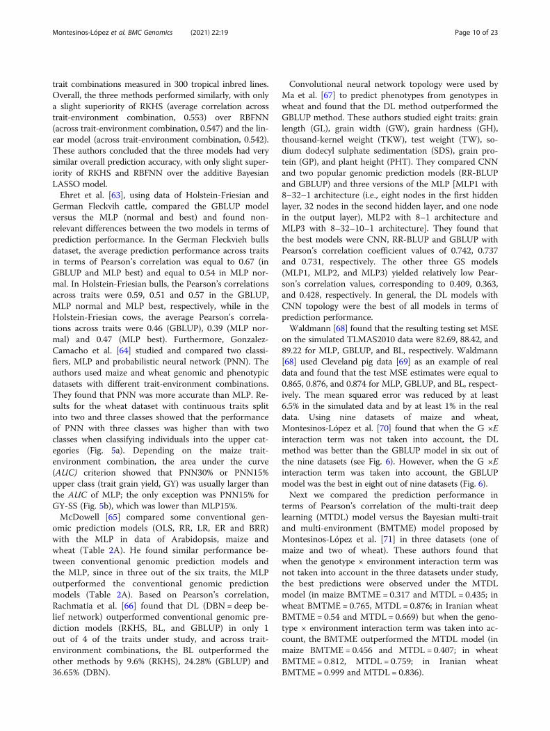
German Fleckvih cattle, compared the GBLUP modelversus the MLP (normal and best) and found non-relevant differences between the two models in terms ofprediction performance. In the German Fleckvieh bullsdataset, the average prediction performance across traitsin terms of Pearson’s correlation was equal to 0.67 (inGBLUP and MLP best) and equal to 0.54 in MLP nor-mal. In Holstein-Friesian bulls, the Pearson’s correlationsacross traits were 0.59, 0.51 and 0.57 in the GBLUP,MLP normal and MLP best, respectively, while in theHolstein-Friesian cows, the average Pearson’s correla-tions across traits were 0.46 (GBLUP), 0.39 (MLP nor-mal) and 0.47 (MLP best). Furthermore, Gonzalez-Camacho et al. [64] studied and compared two classi-fiers, MLP and probabilistic neural network (PNN). Theauthors used maize and wheat genomic and phenotypicdatasets with different trait-environment combinations.They found that PNN was more accurate than MLP. Re-sults for the wheat dataset with continuous traits splitinto two and three classes showed that the performanceof PNN with three classes was higher than with twoclasses when classifying individuals into the upper cat-egories (Fig. 5a). Depending on the maize trait-environment combination, the area under the curve(AUC) criterion showed that PNN30% or PNN15%upper class (trait grain yield, GY) was usually larger thanthe AUC of MLP; the only exception was PNN15% forGY-SS (Fig. 5b), which was lower than MLP15%.McDowell [65] compared some conventional gen-

omic prediction models (OLS, RR, LR, ER and BRR)with the MLP in data of Arabidopsis, maize andwheat (Table 2A). He found similar performance be-tween conventional genomic prediction models andthe MLP, since in three out of the six traits, the MLPoutperformed the conventional genomic predictionmodels (Table 2A). Based on Pearson’s correlation,Rachmatia et al. [66] found that DL (DBN = deep be-lief network) outperformed conventional genomic pre-diction models (RKHS, BL, and GBLUP) in only 1out of 4 of the traits under study, and across trait-environment combinations, the BL outperformed theother methods by 9.6% (RKHS), 24.28% (GBLUP) and36.65% (DBN).

Convolutional neural network topology were used byMa et al. [67] to predict phenotypes from genotypes inwheat and found that the DL method outperformed theGBLUP method. These authors studied eight traits: grainlength (GL), grain width (GW), grain hardness (GH),thousand-kernel weight (TKW), test weight (TW), so-dium dodecyl sulphate sedimentation (SDS), grain pro-tein (GP), and plant height (PHT). They compared CNNand two popular genomic prediction models (RR-BLUPand GBLUP) and three versions of the MLP [MLP1 with8–32–1 architecture (i.e., eight nodes in the first hiddenlayer, 32 nodes in the second hidden layer, and one nodein the output layer), MLP2 with 8–1 architecture andMLP3 with 8–32–10–1 architecture]. They found thatthe best models were CNN, RR-BLUP and GBLUP withPearson’s correlation coefficient values of 0.742, 0.737and 0.731, respectively. The other three GS models(MLP1, MLP2, and MLP3) yielded relatively low Pear-son’s correlation values, corresponding to 0.409, 0.363,and 0.428, respectively. In general, the DL models withCNN topology were the best of all models in terms ofprediction performance.Waldmann [68] found that the resulting testing set MSE

on the simulated TLMAS2010 data were 82.69, 88.42, and89.22 for MLP, GBLUP, and BL, respectively. Waldmann[68] used Cleveland pig data [69] as an example of realdata and found that the test MSE estimates were equal to0.865, 0.876, and 0.874 for MLP, GBLUP, and BL, respect-ively. The mean squared error was reduced by at least6.5% in the simulated data and by at least 1% in the realdata. Using nine datasets of maize and wheat,Montesinos-López et al. [70] found that when the G ×Einteraction term was not taken into account, the DLmethod was better than the GBLUP model in six out ofthe nine datasets (see Fig. 6). However, when the G ×Einteraction term was taken into account, the GBLUPmodel was the best in eight out of nine datasets (Fig. 6).Next we compared the prediction performance in

terms of Pearson’s correlation of the multi-trait deeplearning (MTDL) model versus the Bayesian multi-traitand multi-environment (BMTME) model proposed byMontesinos-López et al. [71] in three datasets (one ofmaize and two of wheat). These authors found thatwhen the genotype × environment interaction term wasnot taken into account in the three datasets under study,the best predictions were observed under the MTDLmodel (in maize BMTME = 0.317 and MTDL = 0.435; inwheat BMTME = 0.765, MTDL = 0.876; in Iranian wheatBMTME = 0.54 and MTDL = 0.669) but when the geno-type × environment interaction term was taken into ac-count, the BMTME outperformed the MTDL model (inmaize BMTME = 0.456 and MTDL = 0.407; in wheatBMTME = 0.812, MTDL = 0.759; in Iranian wheatBMTME = 0.999 and MTDL = 0.836).


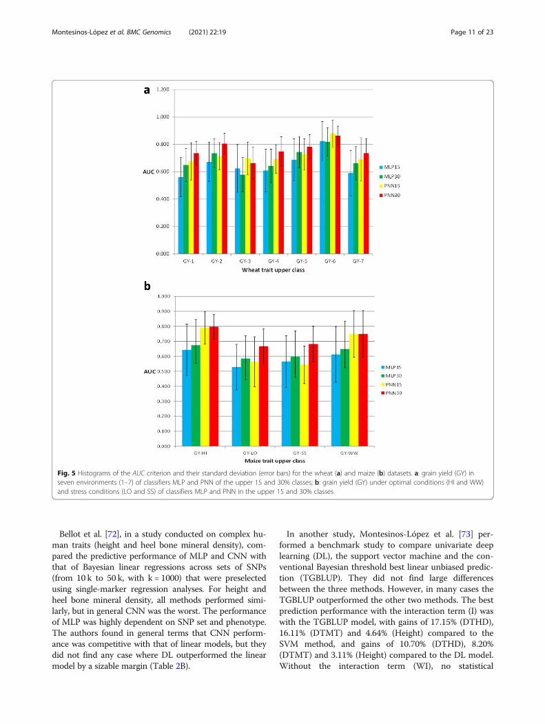
Bellot et al. [72], in a study conducted on complex hu-man traits (height and heel bone mineral density), com-pared the predictive performance of MLP and CNN withthat of Bayesian linear regressions across sets of SNPs(from 10 k to 50 k, with k = 1000) that were preselectedusing single-marker regression analyses. For height andheel bone mineral density, all methods performed simi-larly, but in general CNN was the worst. The performanceof MLP was highly dependent on SNP set and phenotype.The authors found in general terms that CNN perform-ance was competitive with that of linear models, but theydid not find any case where DL outperformed the linearmodel by a sizable margin (Table 2B).

In another study, Montesinos-López et al. [73] per-formed a benchmark study to compare univariate deeplearning (DL), the support vector machine and the con-ventional Bayesian threshold best linear unbiased predic-tion (TGBLUP). They did not find large differencesbetween the three methods. However, in many cases theTGBLUP outperformed the other two methods. The bestprediction performance with the interaction term (I) waswith the TGBLUP model, with gains of 17.15% (DTHD),16.11% (DTMT) and 4.64% (Height) compared to theSVM method, and gains of 10.70% (DTHD), 8.20%(DTMT) and 3.11% (Height) compared to the DL model.Without the interaction term (WI), no statistical

Fig. 5 Histograms of the AUC criterion and their standard deviation (error bars) for the wheat (a) and maize (b) datasets. a: grain yield (GY) inseven environments (1–7) of classifiers MLP and PNN of the upper 15 and 30% classes; b: grain yield (GY) under optimal conditions (HI and WW)and stress conditions (LO and SS) of classifiers MLP and PNN in the upper 15 and 30% classes


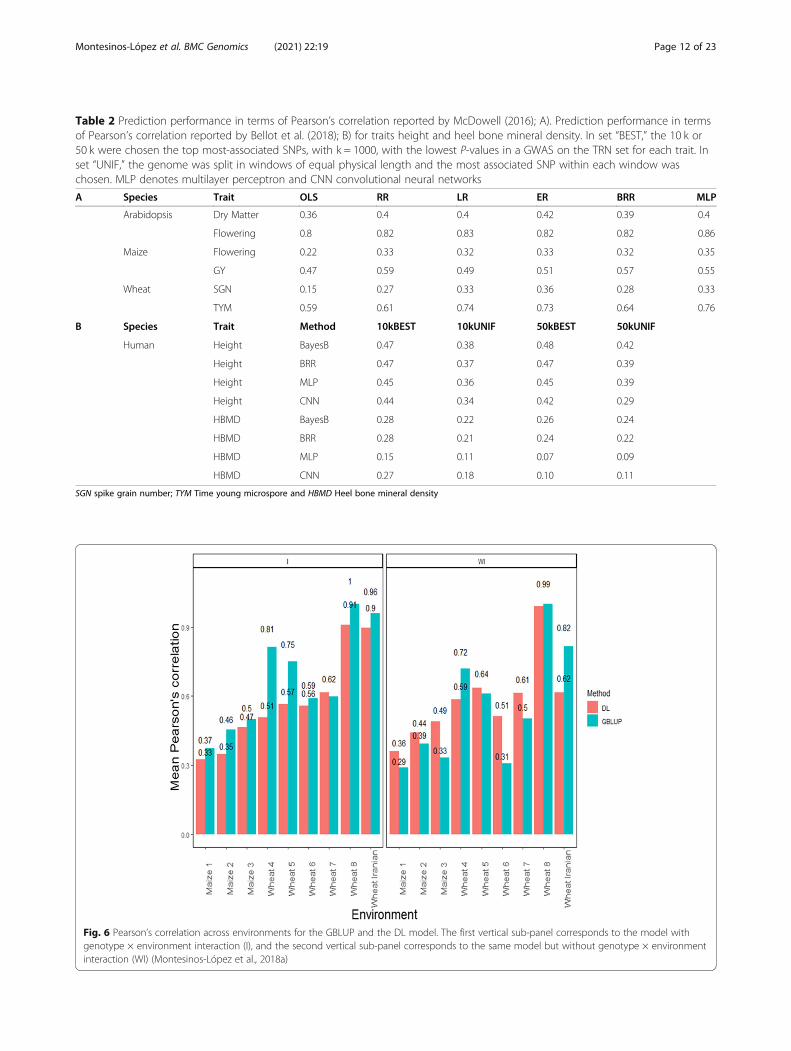
Table 2 Prediction performance in terms of Pearson’s correlation reported by McDowell (2016); A). Prediction performance in termsof Pearson’s correlation reported by Bellot et al. (2018); B) for traits height and heel bone mineral density. In set “BEST,” the 10 k or50 k were chosen the top most-associated SNPs, with k = 1000, with the lowest P-values in a GWAS on the TRN set for each trait. Inset “UNIF,” the genome was split in windows of equal physical length and the most associated SNP within each window waschosen. MLP denotes multilayer perceptron and CNN convolutional neural networks

A Species Trait OLS RR LR ER BRR MLP

Arabidopsis Dry Matter 0.36 0.4 0.4 0.42 0.39 0.4

Flowering 0.8 0.82 0.83 0.82 0.82 0.86

Maize Flowering 0.22 0.33 0.32 0.33 0.32 0.35

GY 0.47 0.59 0.49 0.51 0.57 0.55

Wheat SGN 0.15 0.27 0.33 0.36 0.28 0.33

TYM 0.59 0.61 0.74 0.73 0.64 0.76

B Species Trait Method 10kBEST 10kUNIF 50kBEST 50kUNIF

Human Height BayesB 0.47 0.38 0.48 0.42

Height BRR 0.47 0.37 0.47 0.39

Height MLP 0.45 0.36 0.45 0.39

Height CNN 0.44 0.34 0.42 0.29

HBMD BayesB 0.28 0.22 0.26 0.24

HBMD BRR 0.28 0.21 0.24 0.22

HBMD MLP 0.15 0.11 0.07 0.09

HBMD CNN 0.27 0.18 0.10 0.11

SGN spike grain number; TYM Time young microspore and HBMD Heel bone mineral density

Fig. 6 Pearson’s correlation across environments for the GBLUP and the DL model. The first vertical sub-panel corresponds to the model withgenotype × environment interaction (I), and the second vertical sub-panel corresponds to the same model but without genotype × environmentinteraction (WI) (Montesinos-López et al., 2018a)


differences were found between the three methods(TGBLUP, SVM and DL) for the three traits understudy. Finally, when comparing the best predictions ofthe TGBLUP model that were obtained with the geno-type × environment interaction (I) term and the bestpredictions of the SVM and DL models that were ob-tained without (WI) the interaction term, we found thatthe TGBLUP model outperformed the SVM method by1.90% (DTHD), 2.53% (DTMT) and 1.47% (Height), andthe DL method by 2.12% (DTHD), 0.35% (DTMT) and1.07% (Height).Montesinos-López et al. [74], in a study of durum

wheat where they compared GBLUP, univariate deeplearning (UDL) and multi-trait deep learning (MTDL),found that when the interaction term (I) was taken intoaccount, the best predictions in terms of mean arctan-gent absolute percentage error (MAAPE) across trait-environment combinations were observed under theGBLUP (MAAPE = 0.0714) model and the worst underthe UDL (MAAPE = 0.1303) model, and the second bestunder the MTDL (MAAPE = 0.094) method. However,when the interaction term was ignored, the best predic-tions were observed under the GBLUP (MAAPE =0.0745) method and the MTDL (MAAPE = 0.0726)model, and the worst under the UDL (MAAPE = 0.1156)model; non-relevant differences were observed in thepredictions between the GBLUP and MTDL.Khaki and Wang [75], in a maize dataset of the 2018

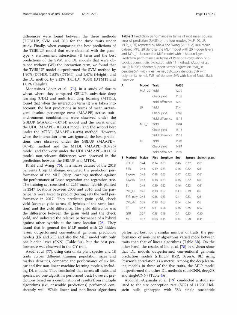
Syngenta Crop Challenge, evaluated the prediction per-formance of the MLP (deep learning) method againstthe performance of Lasso regression and regression tree.The training set consisted of 2267 maize hybrids plantedin 2247 locations between 2008 and 2016, and the par-ticipants were asked to predict (testing set) the yield per-formance in 2017. They predicted grain yield, checkyield (average yield across all hybrids of the same loca-tion) and the yield difference. The yield difference wasthe difference between the grain yield and the checkyield, and indicated the relative performance of a hybridagainst other hybrids at the same location [76]. Theyfound that in general the MLP model with 20 hiddenlayers outperformed conventional genomic predictionmodels (LR and RT) and also the MLP model with onlyone hidden layer (SNN) (Table 3A), but the best per-formance was observed in the GY trait.Azodi et al. [77], using data of six plant species and 18

traits across different training population sizes andmarker densities, compared the performance of six lin-ear and five non-linear machine learning models, includ-ing DL models. They concluded that across all traits andspecies, no one algorithm performed best; however, pre-dictions based on a combination of results from multiplealgorithms (i.e., ensemble predictions) performed con-sistently well. While linear and non-linear algorithms

performed best for a similar number of traits, the per-formance of non-linear algorithms varied more betweentraits than that of linear algorithms (Table 3B). On theother hand, the results of Liu et al. [78] in soybean showthat DL models outperformed conventional genomicprediction models (rrBLUP, BRR, BayesA, BL) usingPearson’s correlation as a metric. Among the deep learn-ing models in three of the five traits, the MLP modeloutperformed the other DL methods (dualCNN, deepGSand singleCNN) (Table 4A).Abdollahi-Arpanahi et al. [79] conducted a study re-

lated to the sire conception rate (SCR) of 11,790 Hol-stein bulls genotyped with 58 k single nucleotide

Table 3 Prediction performance in terms of root mean squareerror of prediction (RMSE) of the four models (MLP_20, LR,MLP_1, RT) reported by Khaki and Wang (2019); A) in a maizedataset. MPL_20 denotes the MLP model with 20 hidden layers,and MPL_1 denotes the MLP model with 1 hidden layer.Prediction performance in terms of Pearson’s correlation of 6species across traits evaluated with 11 methods (Azodi et al.,2019); B). SVR denotes support vector regression. SVR_lindenotes SVR with linear kernel, SVR_poly denotes SVR withpolynomial kernel, SVR_rbf denotes SVR with kernel Radial BasisFunction

A Model Trait RMSE

MLP_20 Yield 12.79

Check yield 11.38

Yield difference 12.4

LR Yield 21.4

Check yield 19.87


MLP_1 Yield 18.04

Check yield 15.18


RT Yield 15.03

Check yield 14.87


B Method Maize Rice Sorghum Soy Spruce Switch-grass

rrBLUP 0.44 0.34 0.63 0.46 0.32 0.61

BRR 0.44 0.39 0.63 0.46 0.32 0.61

BayesA 0.42 0.38 0.63 0.47 0.32 0.61

BayesB 0.43 0.38 0.63 0.46 0.32 0.61

BL 0.44 0.39 0.62 0.46 0.32 0.61

SVR_lin 0.41 0.38 0.62 0.43 0.19 0.6

SVR_poly 0.43 0.38 0.63 0.41 0.33 0.61

SVR_rbf 0.39 0.38 0.63 0.04 0.34 0.6

RF 0.43 0.4 0.58 0.36 0.35 0.57

GTB 0.37 0.38 0.58 0.4 0.33 0.56

MLP 0.17 0.08 0.45 0.44 0.28 0.45


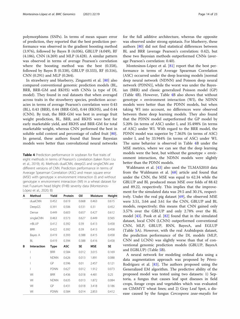
polymorphisms (SNPs). In terms of mean square errorof prediction, they reported that the best prediction per-formance was observed in the gradient boosting method(3.976), followed by Bayes B (4.036), GBLUP (4.049), RF(4.186), CNN (4.269) and MLP (4.428). A similar patternwas observed in terms of average Pearson’s correlationwhere the boosting method was the best (0.358),followed by Bayes B (0.338), GBLUP (0.333), RF (0.316),CNN (0.291) and MLP (0.264).In strawberry and blueberry, Zingaretti et al. [80] also

compared conventional genomic prediction models (BL,BRR, BRR-GM and RKHS) with CNNs (a type of DLmodel). They found in real datasets that when averagedacross traits in the strawberry species, prediction accur-acies in terms of average Pearson’s correlation were 0.43(BL), 0.43 (BRR), 0.44 (BRR-GM), 0.44 (RKHS), and 0.44(CNN). By trait, the BRR-GM was best in average fruitweight prediction, BL, BRR, and RKHS were best forearly marketable yield, and RKHS and BRR-GM for totalmarketable weight, whereas CNN performed the best insoluble solid content and percentage of culled fruit [80].In general, these authors found that linear Bayesianmodels were better than convolutional neural networks

for the full additive architecture, whereas the oppositewas observed under strong epistasis. For blueberry, theseauthors [80] did not find statistical differences betweenBL and BRR (average Pearson’s correlation: 0.42), butthese two Bayesian methods outperformed CNNs (aver-age Pearson’s correlation: 0.40).Montesinos-López et al. [81] report that the best per-

formance in terms of Average Spearman Correlation(ASC) occurred under the deep learning models [normaldeep neural network (NDNN) and Poisson deep neuralnetwork (PDNN)], while the worst was under the Bayes-ian (BRR) and classic generalized Poisson model (GP)(Table 4B). However, Table 4B also shows that withoutgenotype × environment interaction (WI), the NDNNmodels were better than the PDNN models, but whentaking WI into account, no differences were observedbetween these deep learning models. They also foundthat the PDNN model outperformed the GP model by5.20% (in terms of ASC) under I, and 35.498% (in termsof ASC) under WI. With regard to the BRR model, thePDNN model was superior by 7.363% (in terms of ASC)under I, and by 33.944% (in terms of ASC) under WI.The same behavior is observed in Table 4B under theMSE metrics, where we can see that the deep learningmodels were the best, but without the genotype × envir-onment interaction, the NDNN models were slightlybetter than the PDNN models.Waldmann et al. [43] also used the TLMAS2010 data

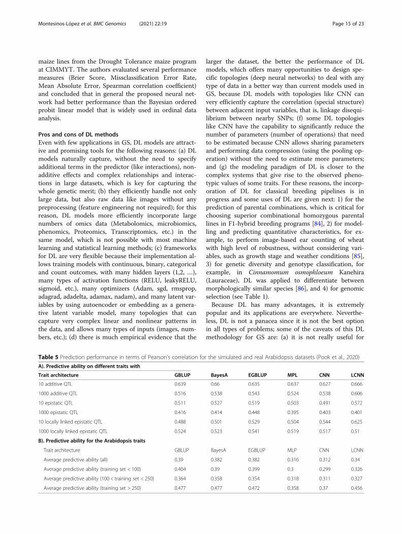
from the Waldmann et al. [68] article and found thatunder the CNN, the MSE was equal to 62.34 while theGBLUP and BL produced mean MSE over folds of 88.42and 89.22, respectively. This implies that the improve-ment for the simulated data was 29.5 and 30.1%, respect-ively. Under the real pig dataset [69], the observed MSEwere 3.51, 3.64 and 3.61 for the CNN, GBLUP and BLmodels, respectively; this means that CNN gained only3.57% over the GBLUP and only 2.78% over the BLmodel [43]. Pook et al. [82] found that in the simulateddataset, local CNN (LCNN) outperformed conventionalCNN, MLP, GBLUP, BNN, BayesA, and EGLUP(Table 5A). However, with the real Arabidopsis dataset,the prediction performance of the DL models (MLP,CNN and LCNN) was slightly worse than that of con-ventional genomic prediction models (GBLUP, BayesAand EGBLUP) (Table 5B).A neural network for modeling ordinal data using a

data augmentation approach was proposed by Pérez-Rodríguez et al. [83]. The authors proposed using theGeneralized EM algorithm. The predictive ability of theproposed model was tested using two datasets: 1) Sep-toria, a fungus that causes leaf spot diseases in fieldcrops, forage crops and vegetables which was evaluatedon CIMMYT wheat lines; and 2) Gray Leaf Spot, a dis-ease caused by the fungus Cercospora zeae-maydis for

Table 4 Prediction performance in soybean for five traits ofeight methods in terms of Pearson’s correlation (taken from Liuet al., 2019); A). Methods dualCNN, deepGS and singleCNN aredifferent versions of CNN. Prediction performance in terms ofAverage Spearman Correlation (ASC) and mean square error(MSE) with genotype × environment interaction (I) and withoutgenotype × environment interaction (WI) in a wheat dataset fortrait Fusarium head blight (FHB) severity data (Montesinos-López et al., 2020; B)

A Method Yield Protein Oil Moisture Height

dualCNN 0.452 0.619 0.668 0.463 0.615

DeepGS 0.391 0.506 0.531 0.31 0.452

Dense 0.449 0.603 0.657 0.427 0.612

singleCNN 0.463 0.573 0.627 0.449 0.565

rrBLUP 0.412 0.392 0.39 0.413 0.458

BRR 0.422 0.392 0.39 0.413 0.458

Bayes A 0.419 0.393 0.388 0.415 0.458

BL 0.419 0.394 0.388 0.416 0.458

B Interaction Type ASC SE MSE SE

I BRR 0.584 0.012 3.015 0.169

I NDNN 0.626 0.013 1.891 0.088

I GP 0.596 0.01 2.457 0.121

I PDNN 0.627 0.012 1.912 0.073

WI BRR 0.436 0.018 4.481 0.25

WI NDNN 0.635 0.013 1.872 0.084

WI GP 0.431 0.018 3.418 0.186

WI PDNN 0.584 0.014 2.853 0.412


maize lines from the Drought Tolerance maize programat CIMMYT. The authors evaluated several performancemeasures (Brier Score, Missclassification Error Rate,Mean Absolute Error, Spearman correlation coefficient)and concluded that in general the proposed neural net-work had better performance than the Bayesian orderedprobit linear model that is widely used in ordinal dataanalysis.

Pros and cons of DL methodsEven with few applications in GS, DL models are attract-ive and promising tools for the following reasons: (a) DLmodels naturally capture, without the need to specifyadditional terms in the predictor (like interactions), non-additive effects and complex relationships and interac-tions in large datasets, which is key for capturing thewhole genetic merit; (b) they efficiently handle not onlylarge data, but also raw data like images without anypreprocessing (feature engineering not required); for thisreason, DL models more efficiently incorporate largenumbers of omics data (Metabolomics, microbiomics,phenomics, Proteomics, Transcriptomics, etc.) in thesame model, which is not possible with most machinelearning and statistical learning methods; (c) frameworksfor DL are very flexible because their implementation al-lows training models with continuous, binary, categoricaland count outcomes, with many hidden layers (1,2, …),many types of activation functions (RELU, leakyRELU,sigmoid, etc.), many optimizers (Adam, sgd, rmsprop,adagrad, adadelta, adamax, nadam), and many latent var-iables by using autoencoder or embedding as a genera-tive latent variable model, many topologies that cancapture very complex linear and nonlinear patterns inthe data, and allows many types of inputs (images, num-bers, etc.); (d) there is much empirical evidence that the

larger the dataset, the better the performance of DLmodels, which offers many opportunities to design spe-cific topologies (deep neural networks) to deal with anytype of data in a better way than current models used inGS, because DL models with topologies like CNN canvery efficiently capture the correlation (special structure)between adjacent input variables, that is, linkage disequi-librium between nearby SNPs; (f) some DL topologieslike CNN have the capability to significantly reduce thenumber of parameters (number of operations) that needto be estimated because CNN allows sharing parametersand performing data compression (using the pooling op-eration) without the need to estimate more parameters;and (g) the modeling paradigm of DL is closer to thecomplex systems that give rise to the observed pheno-typic values of some traits. For these reasons, the incorp-oration of DL for classical breeding pipelines is inprogress and some uses of DL are given next: 1) for theprediction of parental combinations, which is critical forchoosing superior combinational homozygous parentallines in F1-hybrid breeding programs [84], 2) for model-ling and predicting quantitative characteristics, for ex-ample, to perform image-based ear counting of wheatwith high level of robustness, without considering vari-ables, such as growth stage and weather conditions [85],3) for genetic diversity and genotype classification, forexample, in Cinnamomum osmophloeum Kanehira(Lauraceae), DL was applied to differentiate betweenmorphologically similar species [86], and 4) for genomicselection (see Table 1).Because DL has many advantages, it is extremely

popular and its applications are everywhere. Neverthe-less, DL is not a panacea since it is not the best optionin all types of problems; some of the caveats of this DLmethodology for GS are: (a) it is not really useful for

Table 5 Prediction performance in terms of Pearson’s correlation for the simulated and real Arabidopsis datasets (Pook et al., 2020)

A). Predictive ability on different traits with

Trait architecture GBLUP BayesA EGBLUP MPL CNN LCNN

10 additive QTL 0.639 0.66 0.635 0.637 0.627 0.666

1000 additive QTL 0.516 0.538 0.543 0.524 0.538 0.606

10 epistatic QTL 0.511 0.527 0.519 0.503 0.491 0.572

1000 epistatic QTL 0.416 0.414 0.448 0.395 0.403 0.401

10 locally linked epistatic QTL 0.488 0.501 0.529 0.504 0.544 0.625

1000 locally linked epistatic QTL 0.524 0.523 0.541 0.519 0.517 0.51

B). Predictive ability for the Arabidopsis traits

Trait architecture GBLUP BayesA EGBLUP MLP CNN LCNN

Average predictive ability (all) 0.39 0.382 0.382 0.316 0.312 0.34

Average predictive ability (training set < 100) 0.404 0.39 0.399 0.3 0.299 0.326

Average predictive ability (100 < training set < 250) 0.364 0.358 0.354 0.318 0.311 0.327

Average predictive ability (training set > 250) 0.477 0.477 0.472 0.358 0.37 0.456


inference and association studies, since its parameters(weights) many times cannot be interpreted as in manystatistical models; also, since neither feature selectionnor feature importance is obvious, for this reason, theDL methodology inhibits testing hypotheses about thebiological meaning with the parameter estimates; (b)when studying the association of phenotypes with geno-types, it is more difficult to find a global optimum, sincethe loss function may present local minima and maxima;(c) these models are more prone to overfitting than con-ventional statistical models mostly in the presence of in-puts of large dimensions, since to efficiently learn thepattern of the data, more hidden layers and neuronsneed to be taken into account in the DL models; how-ever, there is evidence that these problems can be solvedunder a Bayesian approach and some research is goingin this direction to implement DL models under aBayesian paradigm [87]; but two of the problems underthe Bayesian framework are how to elicit priors and thefact that considerably more computational resources arerequired; (d) considerable knowledge is required forimplementing appropriate DL models and understandingthe biological significance of the outputs, since this re-quires a very complex tuning process that depends onmany hyper-parameters; (e) although there is very user-friendly software (Keras, etc.) for DL, its implementationis very challenging since it depends strongly on thechoice of hyper-parameters, which requires a consider-able amount of time and experience and, of course, con-siderable computational resources [88, 89]; (f) DLmodels are difficult to implement in GS because gen-omic data most of the time contain more independentvariables than samples (observations); and (g) anotherdisadvantage of DL is the generally longer training timerequired [90].

Trends of DL applicationsIn the coming 10 years, DL will be democratized viaevery software-development platform, since DL tools willincorporate simplified programming frameworks for easyand fast coding. However, as automation of DL toolscontinues, there’s an inherent risk that the technologywill develop into something so complex that the averageusers will find themselves uninformed about what is be-hind the software.Nowadays, unsupervised methods (where you only

have independent variables [input] but not dependentvariables [outcomes]) are quite inefficient, but it is ex-pected that in the coming years, unsupervised learningmethods will be able to match the “accuracy and effect-iveness” of supervised learning. This jump will dramatic-ally reduce the cost of implementing DL methods, whichnow need large volumes of labeled data with inputs andoutputs. In the same direction, we expect the

introduction of new DL algorithms that will allow test-ing hypotheses about the biological meaning with par-ameter estimates (good for inference and explainability),that is, algorithms that are not only good for makingpredictions, but also useful for explaining thephenomenon (actual functional biology of the phenotype)to increase human understanding (or knowledge) ofcomplex biological systems.In the coming years, we expect a more fully automated

process for learning and explaining the outputs of imple-mented DL and machine learning models. This meansthat it is feasible to develop systems that can automatic-ally discover plausible models from data, and explainwhat they discovered; these models should be able, notonly to make good predictions, but also to test hypoth-eses and in this way unravel the complex biological sys-tems that give rise to the phenomenon under study.

General considerationsGS as a predictive tool is receiving a lot of attention inplant breeding since it is powerful for selecting candidateindividuals early in time by measuring only genotypic in-formation in the testing set and both phenotypic andgenotypic information in the training set. For this rea-son, this predictive methodology has been adopted forcrop improvement in many crops and countries. GS canperform the selection process more cheaply and in con-siderably less time than conventional breeding programs.This will be key for significantly increasing the geneticgain and reducing the food security pressure since wewill need to produce 70% more food to meet the de-mands of 9.5 billion people by 2050 [1]. Thanks to theever-increasing data generated by industry, farmers, andscholars, GS is expected to improve efficiency and helpmake specific breeding decisions. For this reason, a widerange of analytical methods, such as machine learning,deep learning, and artificial intelligence, are now beingadapted for application in plant breeding to support ana-lytics and decision-making processes [91].The prediction performance in GS is affected by the

size of the training dataset, the number of markers, theheritability, the genetic architecture of the target trait,the degree of correlation between the training and test-ing set, etc. Deep learning can be really powerful for pre-diction if used appropriately, and can help to moreefficiently map the relationship between the phenotypeand all inputs (markers, all remaining omics data, im-aginary data, geospatial and environmental variables,etc.) to be able to address long-standing problems in GSin terms of prediction efficiency.We found that DL has impressive potential to provide

good prediction performance in genomic selection.However, there is not much evidence of its utility forextracting biological insights from data and for making


robust assessments in diverse settings that might be dif-ferent from the training data. Beyond making predic-tions, deep learning could become a powerful tool forsynthetic biology by learning to automatically generatenew DNA sequences and new proteins with desirableproperties.However, more iterative and collaborative experimenta-

tion needs to be done to be able to take advantage of DLin genomic selection. In terms of experimentation, weneed to design better strategies to better evaluate the pre-diction performance of genomic selection in field experi-ments that are as close as possible to real breedingprograms. In terms of collaborative work, we need tostrengthen interdisciplinary work between breeders, bio-metricians, computer scientists, etc., to be able to auto-matically collect (record) more data, the costs of whichcontinue to decrease. The data should include not onlyphenotypic data, but also many types of omics data (meta-bolomics, microbiomics, phenomics using sensors andhigh resolution imagery, proteomics, transcriptomics,etc.), geoclimatic data, image data from plants, data frombreeders’ experience, etc., that are high quality and repre-sentative of real breeding programs. Then, with all col-lected data, we need to design efficient topologies of DLmodels to improve the selection process of candidate indi-viduals. This is feasible because DL models are reallypowerful for efficiently combining different kinds of inputsand reduce the need for feature engineering (FE) the in-put. FE is a complex, time-consuming process whichneeds to be altered whatever the problem. Thus, FE con-stitutes an expensive effort that is data dependent and re-quires experts’ knowledge and does not generalize well[92]. However, this is an iterative process (with trial anderror) where all the members of this network (breeders,biometricians, computer scientists, molecular biologists,etc.) need to contribute their knowledge and experience toreach the main goal. In this way, it is very likely that theprocess of selecting candidate individuals with GS will bebetter than the conventional selection process. For ex-ample, before 2015, humans were better than artificial ma-chines at classifying images and solving many problems ofcomputer vision, but now machines have surpassed theclassification ability of humans, which was considered im-possible only some years ago. In 2016, a robot player beata human player in the famed game AlphaGo, which wasconsidered an almost impossible task. DL also outper-formed 136 of 157 dermatologists in a head-to-head der-moscopic melanoma image classification task [93].However, this task of DL (i.e., selecting the best candi-

date individuals in breeding programs) requires not onlylarger datasets with higher data quality, but also the abilityto design appropriate DL topologies that can combine andexploit all the available collected data. This is importantsince the topologies designed for computer vision

problems are domain specific and cannot be extrapolatedstraightforwardly to GS. For example, in GS most of thetime the number of inputs is considerably larger than thenumber of observations, and the data are extremely noisy,redundant and with inputs of different origins. However,since intelligence relies on understanding and acting in animperfectly sensed and uncertain world, there is still a lotof room for more intelligent systems that can help takeadvantage of all the data that are now being collected andmake the selection process of candidate individuals in GSextremely more efficient.We found no relevant differences in terms of predic-

tion performance between conventional genome-basedprediction models and DL models, since in 11 out of 23studied papers (see Table 1), DL was best in terms ofprediction performance taking into account the genotypeby interaction term; however, when ignoring the geno-type by environment interaction, DL was better in 13out of 21 papers. This in part is explained by the factthat not all data contain nonlinear patterns, not all arelarge enough to guarantee a good learning process, weretuned efficiently, or used the most appropriate architec-ture (examples: shallow layers, few neurons, etc.); inaddition, the design of the training-tuning-testing setsmay not have been optimal, etc. However, we observedthat most of the papers in which the DL models outper-formed conventional GS models were those in whichdifferent versions of CNN were used. There is also a lotof empirical evidence that CNN are some of the besttools for prediction machines when the inputs are rawimages. Some experts attribute the many successfulcommercial applications of DL (which most of the timereach or exceed human performance level) to the build-ing and improvement of this type of topologies that inpart are also responsible for the term deep learningcoined to denote artificial neural networks with morethan one hidden layer. CNNs are different than MLP be-cause they are able to more efficiently capture spatialstructure patterns that are common in image inputs. Forthis reason, CNNs are being very successfully applied tocomplex tasks in plant science for: (a) root and shootfeature identification [94], (b) leaf counting [95, 96], (c)classification of biotic and abiotic stress [97], (d) count-ing seeds per pot [98], (e) detecting wheat spikes [99],and (f) estimating plant morphology and developmentalstages [100], etc. These examples show that DL is play-ing an important role in obtaining better phenotypes inthe field and indirectly affects genomic prediction per-formance. Although DL does not always outperformconventional regression methods, these examples showthat DL is accelerating the progress in prediction per-formance, and we are entering a new era where we willbe able to predict almost anything given good inputs.


In this contribution, we attempt to clarify issues thathave being preventing the use of DL methods at thebreeding level, for instance, that DL is a complete “blackbox” methodology, without much statistical fundamen-tals. There is a widespread sense that implementing DLinto a breeding pipeline is not straightforward without astrong statistical/computing background associated tothe use of super computers - both limiting factors forsome modest breeding programs. Although the learningcurve for DL can be slow, in the Appendix we show amaize toy example with 5 folds cross validation.Finally, since nowadays GS requires high-throughput

genotyping systems and biometrics expertise that mightnot easily accessible to breeding programs in develop-ing countries, increased sharing of genomic resources,genomic data, quantitative genetics and biometricsexpertise between developed countries, developing re-gions and emerging economies will be the key to globalfood security in an era of rapid climate and environ-mental change.

ConclusionsDeep learning is a disruptive technology that has im-mense potential for applications in any area of predictivedata science. An essential requirement is the availabilityof high quality and sufficiently large training data. How-ever, based on the considered publications on the use ofDL for genomic selection, we did not find strong evi-dence for its clear superiority in terms of predictionpower compared to conventional genomic predictionmodels. We obtained evidence that DL algorithms arepowerful for capturing nonlinear patterns more effi-ciently than conventional genomic prediction modelsand for integrating data from different sources withoutthe need for feature engineering. DL algorithms alsohave a lot of potential to improve prediction accuracy bydeveloping specific topologies for the type of data athand in plant breeding programs. For these reasons, it isof paramount importance to adopt this disruptive tech-nology in GS and be able to increase its efficiency andaccuracy. However, DL models cannot be adopted forGS blindly in small training-testing data sets.

Appendix

Maize toy example with 5 folds CV with only oneinner CVrm. (list = ls()).library (lsa).library (keras).library (BMTME).library (plyr).library (tidyr).library (dplyr).

##########Set seed for reproducible results###################.use_session_with_seed(45).#################Loading the MaizeToy Datasets##

#############.data(“MaizeToy”).head (phenoMaizeToy).###########Ordering the data ##################

##############.phenoMaizeToy<−(phenoMaizeToy [order (pheno-

MaizeToy$Env,phenoMaizeToy$Line),])rownames (phenoMaizeToy)=1:nrow (phenoMaizeToy).head (phenoMaizeToy,8).#################Design matrices###############

#####################.LG- cholesky (genoMaizeToy).ZG- model.matrix(~0+as.factor (phenoMaizeToy$Line)).Z.G- ZG %*%LG.Z.E- model.matrix(~0+as.factor (phenoMaizeToy$Env)).ZEG < - model.matrix(~ 0 + as.factor (phenoMaize-

Toy$Line):as.factor (phenoMaizeToy$Env)).G2 < - kronecker (diag (length (unique (phenoMaize-

Toy$Env))), data.matrix (genoMaizeToy)).LG2 < - cholesky(G2).Z.EG < - ZEG %*% LG2.############Selecting the response variable#######

################.Y < - as.matrix (phenoMaizeToy[, −c(1, 2)]).####Training testing sets using the BMTME

package###############.pheno <− data.frame (GID = phenoMaizeToy[, 1],

Env= phenoMaizeToy[, 2],Response=phenoMaizeToy[, 3]).CrossV <− CV.KFold (pheno, DataSetID = ‘GID’, K=5,

set_seed=123).#########Grid of hyperparameters######## ######

####### #####################.Stage <− expand.grid (units_M=seq(33,67,33),epochs_

M = 1000, Dropout = c(0.0,0.05,0.15, 0.25, 0.35)).################Function for averaging the

predictions############.summary. BMTMECV <- function (results, informa-

tion = ‘compact’, digits = 4, ...) {.results % > %.group_by(Environment, Trait, Partition) % > %.summarise (MSE =mean((Predicted-Observed)^2),MAAPE =mean (atan (abs (Observed-Predicted)/abs

(Observed)))) % > %.select (Environment, Trait, Partition, MSE, MAAPE)

% > %.mutate_if(is.numeric, funs (round(., digits))) % > %.as.data.frame() - > presum.presum % > % group_by(Environment, Trait) % > %.


summarise (SE_MAAPE = sd (MAAPE, na.rm. = T)/sqrt(n()), MAAPE =mean (MAAPE, na.rm. = T),SE_MSE = sd (MSE, na.rm. = T)/sqrt(n()), MSE =mean

(MSE, na.rm. = T)) % > %.select (Environment, Trait, MSE, SE_MSE, MAAPE,

SE_MAAPE) % > %.mutate_if(is.numeric, funs (round(., digits))) % > %.as.data.frame() - > finalSum.out <− switch (information,compact = finalSum,complete = presum,extended = {.finalSum$Partition <− ‘All’.presum$Partition <− as.character (presum$Partition).presum$SE_MSE < - NA.presum$SE_MAAPE <- NA.rbind (presum, finalSum).})return (out).}#######Final X and y for fitting the model#######

############.y = (phenoMaizeToy[, 3]).X = cbind(Z.E,Z.G).############Outer Cross-validation##############

#########.digits = 4.Names_Traits = colnames(Y).results = data.frame().t = 1.for (o in 1:5){.tst_set = CrossV$CrossValidation_list[[o]].X_trn = (X[−tst_set,])X_tst = (X [tst_set,])y_trn = (y[−tst_set]).y_tst = (y [tst_set]).nCVI = 1 ####Number of folds for inner CV.i = 1.#########Matrices for saving the output of inner

CV#######################.Tab_pred_MSE =matrix (NA,ncol = length (Stage[,1]),

nrow = nCVI).Tab_pred_Epoch =matrix (NA,ncol = length (Stage[,1]),

nrow = nCVI).Tab_pred_Units = matrix (NA,ncol = length (Stage[,1]),

nrow = nCVI).Tab_pred_Drop =matrix (NA,ncol = length (Stage[,1]),

nrow = nCVI).X_trI = X_trn.y_trI = y_trn.for (stage in seq_len(dim (Stage) [1])) {.X_trII = X_trI.y_trII = y_trI.

units_M < - Stage [stage, 1].epochs_M < - Stage [stage, 2].Drop_per = Stage [stage, 3].build_model<−function() {.model <− keras_model_sequential().model % > %.layer_dense(units = units_M, activation = “relu”, input_

shape = c (dim(X_trII) [2])) % > %.layer_dropout(rate = Drop_per) % > %.layer_dense(units = 1, activation = “relu”).model % > % compile(.loss = “mse”,optimizer = optimizer_adam(),metrics = c(“mse”)).model}.model<−build_model().model % > % summary().print_dot_callback <− callback_lambda(.on_epoch_end = function (epoch, logs) {.if (epoch %% 20 == 0) cat(“\n”).cat(“.”)})########Fitting the model with Early stopping###

####.early_stop <− callback_early_stopping(monitor = “val_

loss”,mode = ‘min’,patience =50).###########Fit of the model for each values of the

grid#################.model_Final<−build_model().model_fit_Final<−model_Final % > % fit(.X_trII, y_trII,epochs = epochs_M, batch_size =72,###shuffled = F,validation_split = 0.2,verbose = 0,callbacks = list (early_stop, print_dot_callback)).###########Saving the output of each hyperpara

meter###################.No.Epoch_Min = length (model_fit_Final$metrics$val_

mean_squared_error).Min_MSE =model_fit_Final$metrics$val_mean_

squared_error[No.Epoch_Min].Tab_pred_MSE[i,stage] =Min_MSE.Tab_pred_Units[i,stage] = units_M.Tab_pred_Epoch[i,stage] = No.Epoch_Min [1].Tab_pred_Drop[i,stage] = Drop_per.}##############Selecting the optimal hyperparameters

##############.Median_MSE_Inner = apply (Tab_pred_MSE,2,median).Units_Inner = apply (Tab_pred_Units,2,max).Drop_Inner = apply (Tab_pred_Drop,2,max).Epoch_Inner = apply (Tab_pred_Epoch,2,median).Pos_Min_MSE = which (Median_MSE_Inner==min

(Median_MSE_Inner)).


Units_O=Units_Inner[Pos_Min_MSE].Epoch_O = Epoch_Inner[Pos_Min_MSE].Drop_O =Drop_Inner[Pos_Min_MSE].###########Refitting the model with the optimal

values#################.model_Sec < −keras_model_sequential().model_Sec % > %.layer_dense(units = Units_O, activation = “relu”, input_

shape = c (dim(X_trn) [2])) % > %.layer_dropout(rate = Drop_O) % > %.layer_dense(units =1).model_Sec % > % compile(.loss = “mean_squared_error”,optimizer = optimizer_adam(),metrics = c(“mean_squared_error”)).ModelFited <−model_Sec % > % fit(.X_trn, y_trn,epochs = Epoch_O, batch_size =30,####### validation_split = 0.2,early_stop,verbose = 0, callbacks = list (print_dot_callback)).####Prediction of testing set

##########################.Yhat =model_Sec % > % predict(X_tst).y_p = Yhat.y_p_tst = as.numeric(y_p).###########Saving the predicctions of each outer-

testing set#################.results<−rbind (results, data.frame (Position = tst_set,Environment = CrossV$Environments [tst_set],Partition = o,Units = Units_O,Epochs = Epoch_O,Drop_Out = Drop_O,Observed = round(y [tst_set], digits), #$response, digits),Predicted = round(y_p_tst, digits),Trait = Names_Traits[t])).cat(“CV = “,o,”\n”).}

Results#############Average of prediction performance##################################.Pred_Summary = summary. BMTMECV (results = results,

information = ‘compact’, digits = 4).Pred_Summary.

AbbreviationsPS: Phenotypic Selection; GS: Genomic Selection; DL: Deep Learning;ML: Machine Learning; GBLUP: Genomic Best Linear Unbiased Predictor;TGBLUP: Threshold Genomic Best Linear Unbiased Predictor; RR-BLUP orrrBLUP: Ridge Regression Best Linear Unbiased Predictor; BMTME: Bayesianmulti-trait and multi-environment; DNN: Deep Neural Network;MLP: Multilayer Perceptron; CNN: Convolutional Neural Networks;ReLu: Rectified linear activation unit; BRR: Bayesian Ridge regression;OLS: Ordinary Least Squares; LR: Linear regression; RKHS: Reproducing KernelHilbert Spaces; RNN: Recurrent Neural Network; PNN: Probabilistic NeuralNetwork; AUC: Area Under the Curve; RBFNN: Kernel Radial Basis Function

Neural Network; RF: Random Forest; RR: Classical Ridge Regression;ER: Classical Elastic Net; DBN: Deep Belief Networks; SVR: Support VectorRegression; UDL: Univariate Deep Learning; MTDL: Multivariate DeepLearning; MAAPE: Mean Arctangent Absolute Percentage Error; ASC: AverageSpearman Correlation; NDNN: Normal Deep Neural Network; PDNN: PoissonDeep Neural Network,; GP: Classic Generalized Poisson model; I: With theInteraction Term; WI: Without the Interaction Term; FE: Feature Engineering;DTHD: Days to heading; DTMT: Days to maturity; GL: Grain length; GW: Grainwidth; GH: Grain hardness; TKW: Thousand-kernel weight; TW: Test weight;SDS: Sodium dodecyl sulphate sedimentation; GP: Grain protein (GP);PH: Plant height

AcknowledgmentsWe thank all scientists, field workers, and lab assistants from NationalPrograms and CIMMYT who collected the data used in this study. Weacknowledge the financial support provided by the Foundation for ResearchLevy on Agricultural Products (FFL) and the Agricultural Agreement ResearchFund (JA) in Norway through NFR grant 267806. We are also thankful for thefinancial support provided by CIMMYT CRP (maize and wheat), the Bill &Melinda Gates Foundation, as well the USAID projects (Cornell University andKansas State University).

Authors’ contributionsThe first author, OAML, had the original idea of writing a review article onDeep Learning drafted the work and wrote the first draft. Correspondingauthors, AML and JC, read and reviewed the first and subsequent drafts ofthe article and assisted the first author to design the review work.Corresponding authors also revised and put together tables and figurestables and figures on the various revised versions of the review and checkedout the correct citations of all 100 references. Authors PPP, JABL, JWRM,SBFF, LSGL, PCSM substantially revised and corrected several versions of themanuscript and checked that reference numbers and references list wascorrectly written in the various version. The author(s) read and approved thefinal manuscript.

Authors’ informationNot applicable

FundingNo special funding for writing this review article.

Availability of data and materialsNot applicable.

Ethics approval and consent to participateNot Applicable.

Consent for publicationNot applicable.

Competing interestsNot applicable.

Author details1Facultad de Telemática, Universidad de Colima, 28040 Colima, Colima,Mexico. 2Departamento de Matemáticas, Centro Universitario de CienciasExactas e Ingenierías (CUCEI), Universidad de Guadalajara, 44430 Guadalajara,Jalisco, Mexico. 3Colegio de Postgraduados, CP 56230 Montecillos, Edo. deMéxico, Mexico. 4Department of Animal Production (DPA), UniversidadNacional Agraria La Molina, Av. La Molina s/n La Molina, 15024 Lima, Peru.5Biometrics and Statistics Unit, International Maize and Wheat ImprovementCenter (CIMMYT), Km 45, CP 52640 Carretera Mexico-Veracruz, Mexico.6School of Mechanical and Electrical Engineering, Universidad de Colima,28040 Colima, Colima, Mexico.


Received: 18 July 2020 Accepted: 10 December 2020

References1. He T, Li C. Harness the power of genomic selection and the potential of

germplasm in crop breeding for global food security in the era with rapidclimate change. Crop J. 2020;8(5):688–700.

2. Qaim M. Role of new plant breeding Technologies for Food Security andSustainable Agricultural Development. Appl Economic Perspect Policy. 2020;42(2):129–50.

3. Bernardo R. Prediction of maize single-cross performance using RFLPs andinformation from related hybrids. Crop Sci. 1994;34:20–5. https://doi.org/10.2135/cropsci1994.0011183X003400010003x.

4. Meuwissen THE, Hayes BJ, Goddard ME. Prediction of total genetic valueusing genome-wide dense marker maps. Genetics. 2001;157:1819–29.

5. Bernardo R. Molecular markers and selection for complex traits in plants:learning from the last 20 years. Crop Sci. 2008;48:1649–64. https://doi.org/10.2135/cropsci2008.03.0131.

6. González-Camacho JM, de los Campos, G., Pérez, P., Gianola, D., Cairns, J.E.,Mahuku, G., et al. Genome-enabled prediction of genetic values using radialbasis function neural networks. Theor Appl Genet. 2012;125:759–71. https://doi.org/10.1007/s00122-012-1868-9.

7. Crossa J, Pérez P, Hickey J, Burgueño J, Ornella L, Cerón-Rojas J, et al.Genomic prediction in CIMMYT maize and wheat breeding programs.Heredity (Edinb). 2013b;112:48–60. https://doi.org/10.1038/hdy.2013.16.

8. Meuwissen T, Hayes B, Goddard M. Accelerating improvement of livestockwith genomic selection. Annu Rev Anim Biosci. 2013;1:221–37. https://doi.org/10.1146/annurev-animal-031412-103705.

9. Wiggans GR, Cole JB, Hubbard SM, Sonstegard TS. Genomic selection indairy cattle: the USDA experience. Annu Rev Anim Biosci. 2017;5:309–27.https://doi.org/10.1146/annurev-animal-021815-111422.

10. Vivek BS, et al. Use of genomic estimated breeding values results in rapidgenetic gains for drought tolerance in maize. Plant Genome. 2017;10:1–8.

11. Môro GV, Santos MF, de Souza Júnior CL. Comparison of genome-wide andphenotypic selection indices in maize. Euphytica. 2019;215:76. https://doi.org/10.1007/s10681-019-2401-x.

12. Smallwood CJ, Saxton AM, Gillman JD, Bhandari HS, Wadl PA, Fallen BD,Hyten DL, Song Q, Pantalone VR. Context-specific Genomic SelectionStrategies Outperform Phenotypic Selection for Soybean Quantitative Traitsin the Progeny Row Stage. Crop Sci. 2019;59(1):54–67.

13. Salam A, Smith KP. Genomic selection performs similarly to phenotypicselection in barley. Crop Sci. 2016;56(6):2871–2881.

14. Harfouche A, et al. Accelerating the domestication of forest trees in achanging world. Trends Plant Sci. 2012;17:64–72.

15. Crossa J, Jarquín D, Franco J, Pérez-Rodríguez P, Burgueño J, Saint-Pierre C,Vikram P, Sansaloni C, Petroli C, Akdemir D, Sneller C. Genomic prediction ofgene bank wheat landraces. G3-Genes Genomes Genet. 2016;6:1819–34.

16. Varshney RK, Thudi M, Pandey MK, Tardieu F, Ojiewo C, Vadez V, WhitbreadAM, Siddique KHM, Nguyen HT, Carberry PS, Bergvinson BD. Acceleratinggenetic gains in legumes for the development of prosperous smallholderagriculture: integrating genomics, phenotyping, systems modelling andagronomy. J Exp Bot. 2018;69:3293–312.

17. Gezan SA, Osorio LF, Verma S, Whitaker VM. An experimental validation ofgenomic selection in octoploid strawberry. Hort Res. 2017;4:16027.

18. de Oliveira EJ, de Resende MD, da Silva Santos V, Ferreira CF, Oliveira, G.A.da Silva, M.S., de Oliveira, L.A., Aguilar-Vildoso, C.I. Genome-wide selection incassava. Euphytica. 2012;187:263–76.

19. Xavier A, Muir WM, Rainey KM. Assessing predictive properties of genome-wide selection in soybeans. G3-Genes-Genomes Genet. 2016;6:2611–6.

20. McElroy MS, Navarro A, Mustiga G Jr, Stack C, Gezan S, Peña G, Sarabia W,Saquicela D, Sotomayor I, Douglas GM, Migicovsky Z, Amores F, Tarqui O,Myles S, Motamayor JC. Prediction of cacao (Theobroma cacao) resistanceto Moniliophthora spp. diseases via genome-wide association analysis andgenomic selection. Front Plant Sci. 2018;9:343.

21. Bhatta M, Gutierrez L, Cammarota L, Cardozo F, Germán S, Gómez-GuerreroB, Pardo MF, Lanaro V, Sayas M, Castro AJ. Multi-trait genomic predictionmodel increased the predictive ability for agronomic and malting qualitytraits in barley (Hordeum vulgare L.). G3-Genes-Genom Genet. 2020;10(2020):1113–24.

22. Liang Z, Gupta SK, Yeh CT, Zhang Y, Ngu DW, Kumar R, Patil HT, MungraKD, Yadav DV, Rathore A, Srivastava RK, Gupta R, Yang J, Varshney RK,

Schnable PSJC. Schnable, phenotypic data from inbred parents can improvegenomic prediction in pearl millet hybrids. G3-Genes Genomes Genet. 2018;8:2513–22.

23. Corak KE, Ellison SL, Simon PW, Spooner DM, Dawson JC. Comparison ofrepresentative and custom methods of generating core subsets of a carrotgermplasm collection. Crop Sci. 2019;59(2019):1107–21.

24. Nyine M, Uwimana B, Blavet N, Hřibová E, Vanrespaille H, Batte M, Akech V,Brown A, Lorenzen J, Swennen R, Doležel J. Genomic prediction in amultiploid crop: genotype by environment interaction and allele dosageeffects on predictive ability in banana. Plant Genome. 2018;11:170090.

25. Mastrodomenico AT, Bohn MO, Lipka AE, Below FE. Genomic selectionusing maize ex-plant variety protection germplasm for the prediction ofnitrogen-use traits. Crop Sci. 2019;59(2019):212–20.

26. Haile JK, Diaye AN, Clarke F, Clarke J, Knox R, Rutkoski J, Bassi FM, PozniakCJ. Genomic selection for grain yield and quality traits in durum wheat. MolBreed. 2018;38:75.

27. Zeng D, Tian Z, Rao Y, Dong G, Yang Y, Huang L, Leng Y, Xu J, Sun C,Zhang G, Hu J. Rational design of high-yield and superior-quality rice. NatPlants. 2017;3:17031.

28. Deomano E, Jackson P, Wei X, Aitken K, Kota R, Pérez-Rodríguez P. Genomicprediction of sugar content and cane yield in sugar cane clones in differentstages of selection in a breeding program, with and without pedigreeinformation. Mol Breeding. 2020;40:38. https://doi.org/10.1007/s11032-020-01120-0.

29. Van Vleck LD. Selection index and introduction to mixed model methods.Boca Raton: CRC Press; 1993.

30. Henderson CR. Sire evaluation and genetic trends. J Animal Sci. 1973;1973(Symposium):10–41.

31. Gianola D, de Los Campos G, Hill WG, Manfredi E, Fernando R. Additivegenetic variability and the Bayesian alphabet. Genetics. 2009;183(1):347–63.

32. Habier D, Fernando RL, Kizilkaya K, Garrick DJ. Extension of the Bayesianalphabet for genomic selection. BMC Bioinformatics. 2011;12(1):186.

33. Gianola D. Priors in whole-genome regression: the Bayesian alphabetreturns. Genetics. 2013;194(3):573–96.

34. Kononenko I, Kukar M. Machine Learning and Data Mining: Introduction toPrinciples and Algorithms. London: Horwood Publishing; 2007.

35. Lewis ND. Deep learning made easy with R. A gentle introduction for datascience. South Carolina: CreateSpace Independent Publishing Platform;2016.

36. Lecun Y, Bengio Y, Hinton G. Deep learning. Nature. 2015. https://doi.org/10.1038/nature14539.

37. Goldberg Y. A primer on neural network models for natural languageprocessing. J Artificial Intell Res. 2016;57(345):420 2016.

38. Makridakis S, Spiliotis E, Assimakopoulos V. Statistical and machine learningforecasting methods: concerns and ways forward. PLoS One. 2018;13(3):e0194889. https://doi.org/10.1371/journal.pone.0194889.

39. Menden MP, Iorio F, Garnett M, McDermott U, Benes CH, Ballester PJ, Saez-Rodriguez J. Machine learning prediction of cancer cell sensitivity to drugsbased on genomic and chemical properties. PLoS One. 2013;8:e61318.

40. Alipanahi B, Delong A, Weirauch MT, Frey BJ. Predicting the sequencespecificities of DNA- and RNA-binding proteins by deep learning. NatBiotechnol. 2015;33:831–8.

41. Tavanaei A, Anandanadarajah N, Maida AS, Loganantharaj R. A DeepLearning Method for Predicting Tumor Suppressor Genes andOncogenes from PDB Structure. bioRxiv. 2017:177378. https://doi.org/10.1101/177378.

42. Angermueller C, Lee HJ, Reik W, Stegle O. DeepCpG: accurate prediction ofsingle-cell DNA methylation states using deep learning. Genome Biol. 2017;18(1):1–13.

43. Waldmann P, Pfeiffer C, Mészáros G. Sparse convolutional neural networksfor genome-wide prediction. Front Genet. 2020;11:25. https://doi.org/10.3389/fgene.2020.00025.

44. Jiang Y, Li C. Convolutional neural networks for image-based high-throughput plant Phenotyping: A review. Plant Phenomics. 2020;2020(4152816):1–22. https://doi.org/10.34133/2020/4152816.

45. Crossa J, Martini JWR, Gianola D, Pérez-Rodríguez P, Jarquin, et al. Deepkernel and deep learning for genome-based prediction of single traits inmultienvironment breeding trials. Front Genet. 2019;10:1168. https://doi.org/10.3389/fgene.2019.01168.

46. Shalev-Shwartz B-D. Understanding machine learning: from theory toalgorithms. New York: Cambridge University Press; 2014.


https://doi.org/10.2135/cropsci1994.0011183X003400010003x

https://doi.org/10.2135/cropsci1994.0011183X003400010003x

https://doi.org/10.2135/cropsci2008.03.0131

https://doi.org/10.2135/cropsci2008.03.0131

https://doi.org/10.1007/s00122-012-1868-9

https://doi.org/10.1007/s00122-012-1868-9

https://doi.org/10.1038/hdy.2013.16

https://doi.org/10.1146/annurev-animal-031412-103705



https://doi.org/10.1007/s10681-019-2401-x

https://doi.org/10.1007/s10681-019-2401-x

https://doi.org/10.1007/s11032-020-01120-0

https://doi.org/10.1007/s11032-020-01120-0

https://doi.org/10.1038/nature14539

https://doi.org/10.1038/nature14539

https://doi.org/10.1371/journal.pone.0194889

https://doi.org/10.1101/177378

https://doi.org/10.1101/177378

https://doi.org/10.3389/fgene.2020.00025


https://doi.org/10.34133/2020/4152816



47. Patterson J, Gibson A. Deep learning: A Practitioner's approach, O'ReillyMedia; 2017.

48. Chollet F, Allaire JJ. Deep learning with R. manning publications, manningearly access program (MEA) first edition; 2017.

49. Berzal F. In: Berzal F, editor. Redes Neuronales and deep learning; 2018.2018, Granada, Spain.

50. Kolmogorov AN. On the representation of continuous functions of severalvariables by superposition of continuous functions of one variable andaddition. Dokl. Akad. Nauk SSSR. 1957;114:953–6.

51. Cybenko G. Approximations by superpositions of sigmoidal functions. MathControl Signal Syst. 1989;2:303–14.

52. Poggio T, Girosi F. Networks for approximation and learning. Proc IEEE.1990;78:1481–97.

53. Hornik K. Approximation capabilities of multilayer feedforward networks.Neural Netw. 1991;4:251–7.

54. Kurkova V. Kolmogorov theorem and multilayer neural networks. NeuralNetw. 1992;5:501–6.

55. Singh AK, Ganapathysubramanian B, Sarkar S, Singh A. Deep learning forplant stress phenotyping: trends and future perspectives. Trends Plant Sci.2018;23:883–98. https://doi.org/10.1016/j.tplants.2018.07.004.

56. Tianqi Chen, Mu Li, Yutian Li, Min Lin, Naiyan Wang, Minjie Wang, TianjunXiao, Bing Xu, Chiyuan Zhang, and Zheng Zhang. (2015). Mxnet: A flexibleand efficient machine learning library for heterogeneous distributedsystems. arXiv:1512.01274.

57. Team, P.C. (2017). Pytorch: tensors and dynamic neural networks in Pythonwith strong GPU acceleration. GitHub pub online: March 22, 2017. https://github.com/pytorch/pytorch.

58. Tokui S, et al. Chainer: a next-generation open source framework for deeplearning. In: Proceedings of the Workshop on Machine Learning Systems(LearningSys) at the 28th Annual Conference on Neural InformationProcessing Systems (NIPS); 2015. http://learningsys.org/papers/LearningSys_2015_paper_33.pdf.

59. Haykin S. Neural networks and learning machines. Pearson prentice hall,Third Edition, New York, USA; 2009.

60. Pérez-Enciso M, Zingaretti LM. A guide on deep learning for complex traitgenomic prediction. Genes. 2019;10:553.

61. Gianola D, Okut H, Weigel KA, Rosa GJ. Predicting complex quantitativetraits with Bayesian neural networks: a case study with Jersey cows andwheat. BMC Genet. 2011;12:87.

62. Pérez-Rodríguez P, Gianola D, González-Camacho JM, Crossa J, Manès Y,Dreisigacker S. Comparison between linear and non-parametric regressionmodels for genome-enabled prediction in wheat. G3 (Bethesda). 2012;2(12):1595–605. https://doi.org/10.1534/g3.112.003665.

63. Ehret A, Hochstuhl D, Krattenmacher N, Tetens J, Klein M, Gronwald W,Thaller G. Short communication: use of genomic and metabolic informationas well as milk performance records for prediction of subclinical ketosis riskvia artificial neural networks. J Dairy Sci. 2015;98:322–9.

64. González-Camacho JM, Crossa J, Pérez-Rodríguez P, et al. Genome-enabledprediction using probabilistic neural network classifiers. BMC Genomics.2016;17:1–16. https://doi.org/10.1186/s12864-016-2553-1.

65. McDowell R. Genomic selection with deep neural networks. GraduateTheses and Dissertations; 2016. p. 15973. https://lib.dr.iastate.edu/etd/15973.

66. Rachmatia H, Kusuma WA, Hasibuan LS. Prediction of maize phenotypebased on whole-genome single nucleotide polymorphisms using deepbelief networks. Related content: Prediction of maize phenotype based onwhole-genome single nucleotide polymorphisms using deep beliefnetworks. IOP Conf Ser J Phys Conf Ser. 2017;835:12003.

67. Ma W, Qiu Z, Song J, Li J, Cheng Q, Zhai J, et al. A deep convolutionalneural network approach for predicting phenotypes from genotypes. Planta.2018;248:1307–18. https://doi.org/10.1007/s00425-018-2976-9.

68. Waldmann P. Approximate Bayesian neural networks in genomicprediction.Genet Selection Evol. 2018;50:70. https://doi.org/10.1186/s12711-018-0439-1.

69. Cleveland MA, Hickey JM, Forni S. A common dataset for genomic analysisof livestock populations. Genes Genom Genet. 2012;2:429–35. https://doi.org/10.1534/g3.111.001453.

70. Montesinos-López A, Montesinos-López OA, Gianola D, Crossa J, Hernández-Suárez CM. Multi-environment genomic prediction of plant traits usingdeep learners with a dense architecture. G3: Genes Genomes Genetics.2018a;8(12):3813–28. https://doi.org/10.1534/g3.118.200740.

71. Montesinos-López OA, Montesinos-López A, Gianola D, Crossa J, Hernández-Suárez CM. Multi-trait, multi-environment deep learning modeling for

genomic-enabled prediction of plant. G3: genes, genomes. Genetics. 2018b;8(12):3829–40.

72. Bellot P, de los Campos, G., Pérez-Enciso, M. Can deep learning improvegenomic prediction of complex human traits? Genetics. 2018;210:809–19.

73. Montesinos-López OA, Vallejo M, Crossa J, Gianola D, Hernández-Suárez CM,Montesinos-López A, Juliana P, Singh R. A benchmarking between deeplearning, support vector machine and Bayesian threshold best linearunbiased prediction for predicting ordinal traits in plant breeding. G3:Genes Genomes Genetics. 2019a;9(2):601–18.

74. Montesinos-López OA, Montesinos-López A, Tuberosa R, Maccaferri M,Sciara G, Ammar K, Crossa J. Multi-trait, multi-environment genomicprediction of durum wheat with genomic best linear unbiased predictorand deep learning methods. Front Plant Sci. 2019;11(10):1–12.

75. Khaki S, Wang L. Crop yield prediction using deep neural networks. FrontPlant Sci. 2019;2019(10):621.

76. Marko O, Brdar S, Pani’c, M., Šaši’c, I., Despotovi’c, D., Kneževi’c, M., et al.Portfolio optimization for seed selection in diverse weather scenarios. PLoSOne. 2017;12:e0184198. https://doi.org/10.1371/journal.pone.0184198.

77. Azodi CB, McCarren A, Roantree M, de los Campos G, Shiu S-H. BenchmarkingParametric and Machine Learning Models for Genomic Prediction of ComplexTraits. Genes Genomes Genetics. 2019;9(11):3691–702.

78. Liu Y, Wang D, He F, Wang J, Joshi T, Xu D. Phenotype prediction andgenome-wide association study using deep convolutional neural networkof soybean. Front Genet. 2019;10:1091. https://doi.org/10.3389/fgene.2019.01091.

79. Abdollahi-Arpanahi R, Gianola D, Peñagaricano F. Deep learning versusparametric and ensemble methods for genomic prediction of complexphenotypes. Genet Sel Evol. 2020;52:12. https://doi.org/10.1186/s12711-020-00531-z.

80. Zingaretti LM, Gezan SA, Ferrão LF, Osorio LF, Monfort A, Muñoz PR,Whitaker VM, Pérez-Enciso M. Exploring deep learning for complex traitgenomic prediction in Polyploid outcrossing species. Front Plant Sci. 2020;11:25. https://doi.org/10.3389/fpls.2020.00025.

81. Montesinos-López OA, Montesinos-López JC, Salazar-Carrillo E, Barrón-LópezJA, Montesinos-López A, Crossa J. A new Poisson deep neural networkmodel for genomic-enabled prediction of count data, the plant genome(submitted); 2020.

82. Pook, T., Freudentha, J., Korte, A., Simianer, H. (2020). Using localconvolutional neural networks for genomic prediction. Frontiers. In Press.

83. Pérez-Rodríguez P, Flores-Galarza S, Vaquera-Huerta H, Montesinos-LópezOA, del Valle-Paniagua DH, Crossa J. Genome-based prediction of Bayesianlinear and non-linear regression models for ordinal data. Plant Genome.2020;13(1):e20021.

84. Khaki S, Khalilzadeh Z, Wang L. Predicting yield performance of parents inplant breeding: A neural collaborative filtering approach. PLoS One. 2020;15:e0233382.

85. Sadeghi-Tehran P, Virlet N, Ampe EM, Reyns P, Hawkesford MJ. DeepCount:in-field automatic quantification of wheat spikes using simple linear iterativeclustering and deep convolutional neural networks. Front Plant Sci. 2019;10:1176.

86. Yang H-W, Hsu H-C, Yang C-K, Tsai M-J, Kuo Y-F. Di_erentiating betweenmorphologically similar species in genusCinnamomum (Lauraceae) using deepconvolutional neural networks. Comput Electron Agric. 2019;162:739–48.

87. Radford NM. Bayesian learning for neural networks. Lecture Notes Stat. 1996;118. https://doi.org/10.1007/978-1-4612-0745-0 ISBN 978-0-387-94724-2.

88. Young SR, Rose DC, Karnowski TP, Lim S-H, Patton RM. Optimizing deeplearning hyper-parameters through an evolutionary algorithm. Proceedingsof the Workshop on Machine Learning in High- Performance ComputingEnvironments - MLHPC ‘15. New York: ACM Press; 2015. p. 1–5. https://doi.org/10.1145/2834892.2834896.

89. Chan M, Scarafoni D, Duarte R, Thornton J, Skelly L. Learning networkarchitectures of deep CNNs under resource constraints. In: IEEE ComputerSociety Conference on Computer Vision and Pattern Recognition Workshops.(IEEE); 2018. p. 1784–91. https://doi.org/10.1109/CVPRW.2018.00222.

90. Kamilaris A, Prenafeta-Boldu FX. Deep learning in agriculture: a survey.Comput Electron Agric. 2018;147:70–90 2018.

91. Ersoz ES, Martin NF, Stapleton AE. On to the next chapter for crop breeding:convergence with data science. Crop Sci. 2020;60(2):639–55.

92. Amara J, et al. A deep learning-based approach for banana leaf diseasesclassification. In: Lecture notes in informatics (LNI); 2017. p. 79–88.Gesellschaft für Informatik.


https://doi.org/10.1016/j.tplants.2018.07.004

https://github.com/pytorch/pytorch

https://github.com/pytorch/pytorch

http://learningsys.org/papers/LearningSys_2015_paper_33.pdf

http://learningsys.org/papers/LearningSys_2015_paper_33.pdf

https://doi.org/10.1534/g3.112.003665

https://doi.org/10.1186/s12864-016-2553-1

https://lib.dr.iastate.edu/etd/15973

https://doi.org/10.1007/s00425-018-2976-9

https://doi.org/10.1186/s12711-018-0439-1

https://doi.org/10.1534/g3.111.001453

https://doi.org/10.1534/g3.111.001453

https://doi.org/10.1534/g3.118.200740

https://doi.org/10.1371/journal.pone.0184198



https://doi.org/10.1186/s12711-020-00531-z

https://doi.org/10.1186/s12711-020-00531-z

https://doi.org/10.3389/fpls.2020.00025

https://doi.org/10.1007/978-1-4612-0745-0

https://doi.org/10.1145/2834892.2834896

https://doi.org/10.1145/2834892.2834896

https://doi.org/10.1109/CVPRW.2018.00222

93. Brinker TJ, Hekler A, Enk AH, Klode J, Hauschild A, Berking C, Schilling B,Haferkamp S, Schadendorf D, Holland-Letz T, Utikal JS, von Kalle C. Deeplearning outperformed 136 of 157 dermatologists in a head-to-headdermoscopic melanoma image classification task. Eur J Cancer. 2019;113:47–54.

94. Pound MP, Atkinson JA, Townsend AJ, et al. Deep machine learningprovides state-of-the-art performance in image-based plant phenotyping.Gigascience. 2017;6(10):1–10.

95. Dobrescu A, Valerio Giuffrida M, Tsaftaris SA. Leveraging multiple datasetsfor deep leaf counting. In: Proceedings of the IEEE International Conferenceon Computer Vision; 2017. p. 2072–9.

96. Giuffrida MV, Doerner P, Tsaftaris SA. Pheno-deep counter: A unified andversatile deep learning architecture for leaf counting. Plant J. 2018;96(4):880–90.

97. Ghosal S, Blystone D, Singh AK, et al. An explainable deep machine visionframework for plant stress phenotyping. Proc Natl Acad Sci U S A. 2018;115(18):4613.

98. Uzal LC, Grinblat GL, Namías R, et al. Seed-per-pod estimation for plantbreeding using deep learning. Comput Electron Agric. 2018;150:196–204.

99. Hasan MM, Chopin JP, Laga H, et al. Detection and analysis of wheat spikesusing convolutional neural networks. Plant Methods. 2018;14(1):100.

100. Wang X, Xuan H, Evers B, Shrestha S, Pless R, Poland J. High-throughputphenotyping with deep learning gives insight into the genetic architectureof flowering time in wheat. GigaScience. 2019;8:1–11.

Publisher’s NoteSpringer Nature remains neutral with regard to jurisdictional claims inpublished maps and institutional affiliations.


A review of deep learning applications for genomic selection

Documents

Transcript of A review of deep learning applications for genomic selection