A relaxation method for two-phase flow models with hydrodynamic closure law

Digital Object Identifier (DOI) 10.1007/s00211-004-0558-1Numer. Math. (2005) 99: 411–440 Numerische

Mathematik

A relaxation method for two-phase flow models withhydrodynamic closure law

Michael Baudin1, Christophe Berthon2, Frederic Coquel3,Roland Masson1, Quang Huy Tran1

1 IFP, 1 et 4 avenue de Bois-Preau, 92852 Rueil-Malmaison Cedex, France2 MAB, Universite de Bordeaux I, 351 cours de la Liberation,

33405 Talence Cedex, France3 Lab. J.-L. Lions, Universite Pierre et Marie Curie, Boıte courrier 187,

75252 Paris Cedex 5

Received September 26, 2002 / Revised version received October 31, 2003Published online: November 26, 2004 – c© Springer-Verlag 2004

Summary. This paper is devoted to the numerical approximation of the solu-tions of a system of conservation laws arising in the modeling of two-phaseflows in pipelines. The PDEs are closed by two highly nonlinear algebraicrelations, namely, a pressure law and a hydrodynamic one. The severe non-linearities encoded in these laws make the classical approximate Riemannsolvers virtually intractable at a reasonable cost of evaluation. We propose astrategy for relaxing solely these two nonlinearities. The relaxation systemwe introduce is of course hyperbolic but all associated eigenfields are linearlydegenerate. Such a property not only makes it trivial to solve the Riemannproblem but also enables us to enforce some further stability requirements, inaddition to those coming from a Chapman-Enskog analysis. The new methodturns out to be fairly simple and robust while achieving desirable positivityproperties on the density and the mass fractions. Extensive numerical evi-dences are provided.

Mathematics Subject Classification (1991): 76T10, 76N15, 35L65, 65M06

Introduction

The purpose of petroleum pipelines is to convey a mixing, made up essen-tially of gas and liquid, over a long distance. In the realm of two-phase flows,there is a wide variety of mathematical models [2,19,23,25]. Those we shall

Correspondence to: Quang Huy Tran

412 M. Baudin et al.

be considering, called Drift-Flux Models, are characterized, on one hand, bya single pressure and a single momentum equation. On the other hand, theDFMs involve two algebraic closures laws: the first one defines the pressureof a mixing gas-liquid as a function of its composition; the second one pre-scribes the hydrodynamic behavior, e.g., the velocity difference between thetwo phases of the flow as a function of the unknowns, such a function beingdefined according to the local incline of the pipeline.

The model considered in this paper describes a two-phase flow inside apipeline with a uniform section but for general pressure and hydrodynamiclaws. When dealing with such a model, the tricky part of the job is to focuson the difficulties associated with the hydrodynamic law which, besides thepressure law, gives rise to the main nonlinearities in the model.

In the flow, the gas (resp. liquid) is characterized by its density ρG (resp.ρL), its velocity vG (resp. vL) and its surface fraction RG ∈ [0, 1] (resp.RL ∈ [0, 1]) with the property RL + RG = 1. The model is governed by thesystem of conservation laws

∂t (ρLRL) + ∂x (ρLRLvL) = 0∂t (ρGRG) + ∂x (ρGRGvG) = 0∂t (ρLRLvL + ρGRGvG) + ∂x (ρLRGv2

L + ρGRGv2G + p) = 0,

(1)

for x ∈ R and t > 0. The unknown is w := (ρLRL, ρGRG, ρLRLvL +ρGRGvG). In addition to the pressure law p = p(w1, w2), assumed to be agiven smooth function, we consider a general algebraic hydrodynamic law[21] of the type

vL − vG = (w), for w1 ≥ 0, w2 ≥ 0, w3 ∈ R,(2)

in order to close (1). The mapping is assumed to be smooth enough. Inpractical situations, turns out to be nonlinear in the unknown w [3,21,30].Consequently, when working with (1)–(2), the velocities vL and vG of thetwo phases must be understood as functions of the unknown w, i.e.,

vL(w) := w3

w1 + w2+ w2

w1 + w2(w),

vG(w) := w3

w1 + w2− w1

w1 + w2(w).(3)

These formulae clearly highlight that the flux function is in full generalityhighly nonlinear!

Besides this observation, such nonlinearities are obviously responsiblefor the basic mathematical properties of the model. For instance, consider-ing the simplest framework, e.g., a pressure law satisfying the assumptionw1

∂p

∂w1+ w2

∂p

∂w2> 0 together with a no-slip hydrodynamic law ≡ 0.

Then, the system (1) can be shown to be hyperbolic (see for instance Benz-oni-Gavage [3]). However, as soon as ≡ 0, the system (1) is generally

A relaxation method for two-phase flow models 413

only conditionally hyperbolic: indeed, for |vL − vG| = || large enoughthe hyperbolicity property is lost. To cap it all, an arbitrary hydrodynamicclosure (2) precludes the existence of additional non trivial conservation lawfor smooth solution of (1)–(2). In other words, without restrictive physicalassumptions (such as ≡ 0), the system under consideration cannot beendowed with an entropy pair.

Let us now turn to the issue of computing approximated solutions for(1)–(2). The algebraic complexity due to the above mentioned nonlinearitiesprevents us from using classical approximate Riemann solvers [10–13,22],simply because these methods, which make heavy use of the eigen-struc-ture of the exact Jacobian matrix, would become overwhelmingly expen-sive in a real-life context. Notice that even for simpler methods, like thewell-known Rusanov scheme, one needs an estimate of the largest eigen-value of the Jacobian matrix. In the present work, we propose a strategyof relaxation of the two main nonlinearities involved in (1)–(2). Since noentropy pair is known for the system under consideration, our approachcannot enter the general relaxation theory developped by Liu [18], Chenet al. [5]. We are thus led to adopt the framework proposed by Whitham[28] which relies on suitable Chapman-Enskog expansions. As expected,such expansions will provide us with some sub-characteristic like condi-tions expressing that some diffusion matrix must remain non-negative [5,18].

The scheme we propose below differs from the classical relaxation schemedeveloped by Jin and Xin [29] (recently studied by Natalini [20], Aregba andNatalini [1] in the scalar cases) since we do not relax every nonlinearity. Thispartial relaxation procedure is more physically relevant and have been alreadyproposed by various authors, in particular Jin and Slemrod [14,15], Coqueland Perthame [8] and Coquel et al. [7]. Relaxing solely the pressure law andthe hydrodynamic law will tremendously facilitate the Chapmann-Enskoganalysis. It will in particular enable us to exhibit precise and simple stabilityconditions for our relaxation model. Another feature of the scheme we pro-pose is that positivity for the partial densities is ensured. This is achieved byextending Larrouturou’s ideas [16].

This paper is outlined as follow. In the next section, the relaxation model isproposed and its main properties are analyzed. This relaxation model involvestwo constant speeds of propagation (understood as free parameters in our pro-cedure), the accurate definition of which will be carried out on the grounds ofseveral stability requirements. In the second section, a fairly simple approx-imate Riemann solver is derived within the frame of relaxation methods.A special attention is paid to preserving positivity of the densities. In thisrespect, a suitable and simple lower bound for the two constant speeds ofpropagation of the model is shown to exist. Finally in the last section, somenumerical results are discussed.


1 A relaxation model

In order to conveniently relax the main nonlinearities involved in the systemunder consideration, namely, the pressure law and the hydrodynamic one,we first perform a conservative change of variables which thus preserves theweak solutions of (1)–(2). To this end, let us consider the total density of themixing ρ = ρLRL + ρGRG, the total momentum ρv = ρLRLvL + ρGRGvG

and ρY where Y denotes the mass fraction of one of the two phases. To fixideas and without restriction, we choose Y = ρGRG

ρ(so that 1 − Y = ρLRL

ρ).

The natural phase space associated with such variables then reads

Ω = u = (ρ, ρv, ρY ) ∈ R

3; ρ > 0, v ∈ R, Y ∈ [0, 1].

With some little abuse, both the pressure law p and the hydrodynamic clo-sure will keep their previous notations when expressed in terms of the newvariable u. In order to simplify the notations, let us introduce

σ(u) = ρY (1 − Y )(u) and P(u) = p(u) + ρY (1 − Y )(u)2.(4)

Equipped with this admissible change of variables, we state

Lemma 1 Weak solutions of the system (1)–(2) equivalently obey the con-servative system

∂t (ρ) + ∂x(ρv) = 0

∂t (ρv) + ∂x(ρv2 + P(u)) = 0

∂t (ρY ) + ∂x(ρYv − σ(u)) = 0.

(5)

From now on, the system (5) will be given the condensed form

∂tu + ∂xF(u) = 0, for t > 0, x ∈ R,(6)

where the flux F : Ω → R3 finds a clear definition. The system (6) is referred

to as the equilibrium system in Eulerian coordinates.

Proof The two functions σ and P clearly encode the most severe nonlinear-ities in the system (5). The first equation in (5) readily follows when addingthe two mass conservation laws in (1). Straightforward calculations yield thetwo identities vL = v + Y(u) and vG = v − (1 − Y )(u), from which thelast equation in (5) is obtained. We conclude the equivalence statement byarguing again from the above two identities to get

ρLRLv2L + ρGRGv2

G = ρ(1 − Y ) (v + Y)2 + ρY (v − (1 − Y ))2

= ρv2 + ρY (1 − Y )2.(7)

which is the desired result.


1.1 Design of the relaxation system

It is helpful to rewrite the system (5) in terms of the Lagrangian coordinatesbased on the density ρ and the velocity v. Let us set τ = 1/ρ, and define theLagrangian mass coordinate y by dy = ρdx − ρvdt . Then the equilibriumsystem in Lagrangian coordinates [24,12] writes

∂tτ − ∂yv = 0

∂tv + ∂yP (u) = 0

∂tY − ∂yσ (u) = 0.

(8)

We decide to approximate the solutions of (5) by those of a relaxation system,obtained by replacing the nonlinearities σ(u) and P(u) by two new variables and . These are, of course, intended to coincide respectively with σ(u)

and P(u) in the limit of some relaxation parameter, say, λ. We consider therelaxation model

∂tτλ − ∂yv

λ = 0,

∂tvλ + ∂y

λ = 0,

∂tλ + a2∂yv

λ = λ(P (u) − λ),

∂tYλ − ∂y

λ = 0,

∂tλ − b2∂yY

λ = λ(σ(u) − λ),

(9)

where the superscript λ reminds the dependency of the solution on the param-eter λ. Then we return in the original frame to obtain

∂t (ρ)λ + ∂x(ρv)λ = 0,

∂t (ρv)λ + ∂x(ρv2 + )λ = 0,

∂t (ρ)λ + ∂x(ρv + a2v)λ = λρλ(P (uλ) − λ),

∂t (ρY )λ + ∂x(ρYv − )λ = 0,

∂t (ρ)λ + ∂x(ρv − b2Y )λ = λρλ(σ (uλ) − λ).

(10)

For simplicity, the superscript λ will be omitted most of the time. The relax-ation system (10) will be given hereafter the convenient abstract form

∂tv + ∂xG(v) = λR(v), for t > 0, x ∈ R,(11)

where both the flux function G and the relaxation terms R receive cleardefinitions. The associated admissible state space V reads

V = v = t (ρ, ρv, ρ, ρY, ρ) ∈ R

5;ρ > 0, v ∈ R, ∈ R, Y ∈ [0, 1], ∈ R .(12)

In (10), a and b denote two real free parameters in the relaxation procedurewe propose. All along the present work, we shall pay a central attention to


the specification of these two constants, on the ground of several stabilityrequirements. In this respect, successive and sharper definitions for such apair will be given in the forthcoming sections. The final definition of (a, b)

is postponed to Section 2.4.The next statement will be useful in the forthcoming developments.

Lemma 2 Smooth solutions of (10) satisfy the non-conservative system

∂tτ + v∂xτ − τ∂xv = 0,

∂tv + v∂xv + τ∂x = 0,

∂t + v∂x + a2τ∂xv = λ(P (u) − ),

∂tY + v∂xY − τ∂x = 0,

∂t + v∂x − b2τ∂xY = λ(σ(u) − ).

(13)

The proof of this easy result is left to the reader. Let us observe that theLagrangian form (9) of our relaxation model is nothing else but a first orderquasi-linear system with singular perturbations. In this respect, the relaxa-tion procedure we propose now finds clear relationships with the Xin and Jinapproach [29] but at the expense of a Lagrangian transformation. To go fur-ther, let us set the relaxation parameter λ to zero. Then, the system (9) splitsitself into two independent linear hyperbolic systems, one in the unknowns(τ, v, ), the other in (Y, ). The first group of unknowns can be associ-ated respectively with the specific volume, the velocity and the pressure ofan hypothetic gas where the parameter a would play the role of a (constant)Lagrangian sound speed. Likewise, the second pair would characterize thespecific volume Y and the velocity of a hypothetic isentropic gas withthe parameter b as sound speed. These two (linear) hypothetic gas dynamicssystems have connections with the recent works by Bouchut [4], Despres [9]and Suliciu [26]; all these works being primarily devoted to the Lagrangiansetting. Our approach, already introduced in other contexts (see [8] and [7]),could be thus understood as an extension to the Eulerian framework.

Let us now state the basic properties of the Eulerian form (10).

Lemma 3 Let (a, b) be a pair of strictly positive real numbers For anyv ∈ V , the first order system extracted from (10) admits five real eigenvalues(τ = 1/ρ) v, v ± aτ, v ± bτ, and five linearly independent correspond-ing eigenvectors. Consequently, the first order extracted system from (10) ishyperbolic on V . Moreover, each eigenvalue is associated with a linearlydegenerate field.

Linear degeneracy of each of the fields is a by-product of the derivationprinciple of the nonlinear relaxation model (10). Such a property is expected[27] from the Lagrangian form (9). It is actually desired since it makes itstraightforward for us to solve the Riemann problem associated with (10)when λ = 0 (see indeed Proposition 3, Section 2.1).


Proof The hyperbolicity properties of a first order nonlinear system areknown to be independent [12] from a given change of variables. It is thenconvenient to use the non conservation form (13) to immediately derive therequired eigenvalues. Easy calculations show that the vectors ri(v), i =1, . . . , 5, given by

(1, 0, 0, 0, 0), (ρ, ±aτ, a2τ, 0, 0) and (0, 0, 0, 1, ∓b),(14)

are respectively right eigenvectors for the eigenvalues λi(v): v, v ± aτ , andv ± bτ . These vectors are clearly independent provided that the parametersa and b are not zero. It is easily seen that ∇λi(v) · ri(v) = 0 for i = 1, . . . , 5for all v ∈ V . Such a property expresses, after Lax [17], the linear degeneracyof all the fields under consideration.

1.2 Chapman-Enskog expansion

The properties stated in Lemma 3 hold true regardless of the choice of anon zero pair (a, b) (say, strictly positive for definiteness). However, it isknown after the works by Liu [18], Chen et al. [5] that some compatibilityconditions must be satisfied by the original equilibrium system (1) and itsrelaxation approximation (10). These conditions are actually needed to pre-vent the relaxation approximation procedure from instabilities as λ goes toinfinity. They are usually referred to as sub-characteristic like conditions afterWhitham [28]. It is therefore expected that the parameters a and b must befixed in order to fulfill such stability requirements. There exist various waysto exhibit the needed conditions. A powerful one requires the existence ofcompatible Lax entropy pairs for both the equilibrium system and its relaxa-tion approximation [5]. However, as was already explained, the equilibriumsystem under consideration (1) fails to admit additional non trivial conser-vation laws for general hydrodynamic closure (2). This lack for equilibriumentropy pair thus forbids us to enter the general framework proposed in [5].

A weaker approach [28]) is based on the derivation of the first orderasymptotic equilibrium system. In our relaxation framework, its derivationis based on a Chapman-Enskog expansion of small departures vλ from thelocal equilibrium u:

λ = P(uλ) + λ−1λ1 + O (

λ−2) ,(15a)

λ = σ(uλ) + λ−1λ1 + O (

λ−2) .(15b)

In (15), the dependency of the first order correctors λ1 and λ

1 in λ comesfrom the fact that they actually depend on both the equilibrium unknown uλ

and its space derivative.After substituting (15) into (10) and neglecting higher


order terms, we classically end up with the first order asymptotic equilibriumsystem with the generic form (see Proposition 2 for a brief derivation)

∂tuλ + ∂xF(uλ) = λ−1∂x(D(a,b)(uλ)∂xuλ),(16)

where the flux function F coincides with the one in (6) and where the tensorD(a,b) will be given an explicit form hereafter. According to the notations,this tensor does actually depend on the free parameters a and b.

Now, the stability conditions to be put on the pairs (a, b) clearly comefrom the requirement that the first-order correction operator in (16) must bedissipative relatively to the zero-order approximation (6). Such conditionsmay be obtained by establishing the L2-stability of the constant coefficientproblem obtained by linearizing (16) in the neighborhood of any equilib-rium state u. In other words, for all admissible states u, all eigenvalues of thematrix +iξ∇uF(u)−λ−1ξ 2D(a,b)(u) for all ξ ∈ R, should have negative realparts [24]. The algebraic complexity of the Jacobian matrix ∇uF for generalhydrodynamic closures (2) virtually makes such a criterion intractable forour numerical purposes. As a consequence, we adopt the weaker conditionon (a, b) according to which the eigenvalues of the tensor D(a,b)(u) must benon-negative real numbers for all the states u under consideration. The mainresult of this section actually shows that it is always possible to fulfill thisstability requirement.

Proposition 1 There exist four smooth mappings A, B, C, D : Ω → R

(explicitly known and detailed below) such that for any given u ∈ Ω , thetensor D(a,b) meets the form

D(a,b)(u) = 1

ρ2

0 0 0× a2 − A(u) C(u)

× D(u) b2 − B(u)

.(17)

This tensor therefore always admits one zero eigenvalue. For any given u ∈Ω , the two other non trivial eigenvalues of D(a,b)(u) are positive iff the setof inequalities

[(a2 − A(u)

) − (b2 − B(u)

)]2 ≥ −4C(u)D(u),(a2 − A(u)

) (b2 − B(u)

) ≥ C(u)D(u),(a2 − A(u)

) + (b2 − B(u)

) ≥ 0.(18)

is satisfied by pair (a, b).

Let us observe that whatever the signs of the bounded real numbers A(u),B(u), C(u) and D(u), the parameters a and b can be always chosen largeenough so that (18) is valid. We shall give below a sharper and more conve-nient characterization of admissible pairs (a, b).


Assuming first that the tensor D(a,b) meets the above mentioned form.The set of inequalities (18) obviously comes from the fact that the two nontrivial eigenvalues of D(a,b)(u) are roots of the quadratic equation

[λ − (

a2 − A(u))] [

λ − (b2 − B(u)

)] − C(u)D(u) = 0.(19)

Requiring these roots to be positive real numbers is equivalent first to en-force the discriminant of this equation to remain non negative, hence the firstinequality in (18), then to enforce both the sum and the product of the rootsto be non negative, hence the last two inequalities.

The computation of D(a,b)(u)’s entries relies on easy but cumbersomealgebra. It turns out that expressing the main nonlinearities of the problemin terms of the variables (τ, v, Y ) instead of the conservative one leads tosimpler calculations. For the sake of simplicity and with some abuse in thenotations, nonlinear functions (like the pressure or the hydrodynamic law)will be given the same notation when expressed in both types of variables.The final results of the calculations are gathered in the following

Proposition 2 The first order asymptotic equilibrium system (16) reads

∂t (ρ)λ + ∂x (ρv)λ = 0,

∂t (ρv)λ + ∂x (ρv2 + P(u)))λ = λ−1∂x

(D1(uλ) · ∂xuλ

),

∂t (ρY )λ + ∂x (ρYv − σ(u))λ = λ−1∂x

(D2(uλ) · ∂xuλ

).

(20)

To define the smooth mappings D1, D2 : Ω → R3, let us set

C(u) = −Pv(u)PY (u) + PY (u)σY (u)(21)

D(u) = −στ (u) + σv(u)Pv(u) − σY (u)σv(u)(22)

A(u) = −Pτ (u) + P 2v (u) − PY (u) σv(u)(23)

B(u) = σ 2Y (u) − σv(u) PY (u)(24)

where subscripts denote partial derivatives. Then,

D1(u) = 1

ρ2

×a2 − A(u)

C(u)

and D2(u) = 1

ρ2

×D(u)

b2 − B(u)

.

Remark 1 The σ 2Y term in B is the one that appears in the relaxation of

the scalar equation ∂tY − ∂yσ (Y ) = 0. The Pτ term in A is the one thatappears in the relaxation of the Isothermal Euler system. This is natural sincethe Lagrangian structure of the system (5) is (8) which is close to this twomodels. The others terms which appear in (21–24) come therefore from thecoupling between the equations.


Proof Considering smooth solutions of the relaxation system (10), the re-laxed pressure and the velocity are easily seen to satisfy

∂t + v∂x + a2τ∂xv = λ(P (u) − ),

∂t + v∂x − b2τ∂xY = λ(σ(u) − ).

Plugging the expansions (15) into the two above equations and dropping thehigher order terms, we end up with

∇uP(u)∂tu + v∂xP (u) + a2τ∂xv = −1 + O (λ−1) ,

∇uσ(u)∂tu + v∂xσ (u) − b2τ∂xY = −1 + O (λ−1) .(25)

In the above equations, we wish to turn time derivatives into space deriva-tives. In that aim, it suffices to express ∂tu in terms of the time derivatives ofρ, v and Y and then to use the identities

∂tρ = −v∂xρ − ρ∂xv,

∂tv = −v∂xv − τ∂xP (u)

∂tY = −v∂xY + τ∂xσ (u)

(26)

which are similar to those stated in Lemma 2. Using these equalities in (25)yields after lengthy calculations (which we shall not not report here)

1 = −D1(u) · ∂xu, 1 = +D2(u) · ∂xu.(27)

To complete the proof, let us consider the following set of PDE’s extractedfrom the relaxation model (10)

∂t (ρ)λ + ∂x (ρvλ) = 0,

∂t (ρv)λ + ∂x (ρv2 + )λ = 0,

∂t (ρY )λ + ∂x (ρYv − )λ = 0.

(28)

It is then sufficient to plug the expansions (15) into these equations to obtain

∂t (ρ)λ + ∂x (ρv)λ = 0,

∂t (ρv)λ + ∂x (ρv2 + P(u))λ = −λ−1∂x1 + O (λ−2

),

∂t (ρY )λ + ∂x (ρYv − σ(u))λ = λ−1∂x1 + O (λ−2

),

(29)

which is nothing but the expected system (20), thanks to (27). To conclude this section, let us notice that a sharp characterization for a givenu ∈ Ω of all the pairs (a, b) satisfying the stability condition (18) obviouslydepends on the sign of A(u), B(u), C(u) and D(u). For numerical purposes,it seems convenient to propose a characterization of admissible pairs whichstays free from signs consideration. In that aim, let us prove the followinglemma.


Lemma 4 Let us defineγ (u) = |C(u)D(u)|. Let us define the couple (a−, b−)

by

a−(u) = (√

2 + 1)√

γ (u), b−(u) = (√

2 − 1)√

γ (u),(30)

and the couple (a−, b−) by

a−(u) =√

a−(u) + A(u), b− =√

b−(u) + B(u).(31)

Then the conditions (18) are satisfied.

Proof The idea consists in making the change of variables a = a2 − A andb = b2 − B. The conditions (18) now become

(a − b)2 + 4 CD ≥ 0(32)

ab − CD ≥ 0(33)

a + b ≥ 0.(34)

It is easy to see that a sufficient condition for (32)–(34) is

(a − b)2 − 4 γ ≥ 0(35)

ab − γ ≥ 0(36)

a + b ≥ 0,(37)

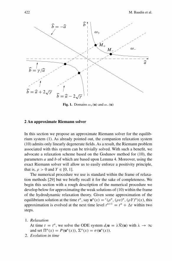
with γ = |CD|. Figure 1 depicts the solutions of this system of inequalitiesin the plane (a, b).

We see that the equalities associated with the inequalities (35)–(36) havealways 4 intersection points but the inequality (37) picks up only two of these,namely, M+ and M−. Let ω+ (resp. ω−) be the domain associated with M+(resp. M−). In ω+ ∪ ω−, which contains all solutions of the system (35–37),we select (a, b) to be as small as possible in order to minimize the numericaldissipation. The optimal points are precisely M+ and M−.

It is simple to compute the coordinates of M− because the correspondinga is the positive solution of the equation γ

a= a −2

√γ , which can be written

a2 − 2√

γ a − γ = 0. Therefore, the coordinates of M− are

a− =(√

2 + 1) √

γ and b− =(√

2 − 1) √

γ .(38)

Similarly, the coordinates of M+ are

a+ =(√

2 − 1) √

γ and b+ =(√

2 + 1) √

γ .(39)

Obviously, a− > b− whereas a+ < b+. But we are primarily interested in theslow waves. This is why we prefer to minimize b. Our choice is the couple(a−, b−).

In the next section, devoted to the numerical approximation of the solu-tions of the equilibrium system (5), the above sets ω+(u) and ω−(u) will playan important role.


a

bb = −a

b = γ /a

M+M−

ω+

ω−

b = a − 2√

γb = a + 2

√γ

Fig. 1. Domains ω+(u) and ω−(u)

2 An approximate Riemann solver

In this section we propose an approximate Riemann solver for the equilib-rium system (1). As already pointed out, the companion relaxation system(10) admits only linearly degenerate fields. As a result, the Riemann problemassociated with this system can be trivially solved. With such a benefit, weadvocate a relaxation scheme based on the Godunov method for (10), theparameters a and b of which are based upon Lemma 4. Moreover, using theexact Riemann solver will allow us to easily enforce a positivity principle,that is, ρ > 0 and Y ∈ [0, 1].

The numerical procedure we use is standard within the frame of relaxa-tion methods [29] but we briefly recall it for the sake of completeness. Webegin this section with a rough description of the numerical procedure wedevelop below for approximating the weak solutions of (10) within the frameof the hydrodynamic relaxation theory. Given some approximation of theequilibrium solution at the time tn, say un(x) = t (ρn, (ρv)n, (ρY )n)(x), thisapproximation is evolved at the next time level tn+1 = tn + t within twosteps.

1. RelaxationAt time t = tn, we solve the ODE system dtu = λR(u) with λ → ∞and set n(x) = P(un(x)), n(x) = σ(un(x)).

2. Evolution in time


We take λ = 0 and solve the system of partial differential equations∂tv + ∂xG(v) = 0 in order to go to time tn+1 = tn + t .

Remark 2 Xin and Jin [29] make a distinction between the “relaxing scheme”in which one uses a small fixed value of ε = 1

λ(for example ε = 10−8) and

the relaxed scheme which is the ε = 0 limit of the relaxing schemes. Ourscheme is of the second class.

2.1 Relaxation scheme

We now give a thorough description of the numerical method. Let t and x

be respectively the time and space steps. We define the time levels tn = n t

for n ∈ N and the cell interface location xi+1/2 = (i + 1/2) x for i ∈ Z.We consider piecewise constant approximate equilibrium solutions uh(x, t) :R × R+ → Ω under the classical form

uh(x, t) = uni = T

(ρn

i , (ρv)ni , (ρY )ni),

for (x, t) ∈]xi−1/2, xi+1/2[×[tn, tn+1[.(40)

At t = 0, we set

u0i = 1

x

∫ xi+1/2

xi−1/2

T(ρ0(x), (ρv)0(x), (ρY )0(x)

)dx.

In order to advance the approximate equilibrium solution in time, we defineanother function vh(x, t) : R × R+ → V which is also piecewise constantat each time level tn. In each slab R × [tn, tn+1[ , the function vh(x, tn + t),with 0 < t < t , is the weak solution of the Cauchy problem for (10)obtained with λ = 0 while prescribing the following initial data given forx ∈]xi−1/2, xi+1/2[

vh(x, tn) = vni = t ((ρ)ni , (ρv)ni , (ρ)ni , (ρY )ni , (ρ)ni )(41)

with (ρ)ni := ρni P (un

i ) and (ρ)ni := ρni σ (un

i ). When t is small enough,i.e., under the CFL condition

t

xmax |µi(vh)| ≤ 1

2,(42)

where (µi)1≤i≤5 denotes the eigenvalues defined in Lemma 3, the functionvh is classically obtained by solving a sequence of local Riemann problemswithout interaction, located at each cell interface xi+1/2.

The CFL restriction (42) will allow us to use the celebrated Harten, LaxandVan Leer [13] formalism which will turn out to be particularly well-suitedto our forthcoming purpose, that is, a local definition of the pair (a, b) at eachcell interface xi+1/2. Following Coquel and Perthame [8], let uL and uR in


Ω be two given equilibrium states and define vL = v(uL) and vR = v(uR)

according to (41). We may think of choosing vL = vni and vR = vn

i+1 whenconsidering the interface xi+1/2. Let us choose a pair of parameters (a, b) forcompleting the definition of the relaxation system (10). Precise conditionson these parameters will be introduced later on. Let us keep in mind that thepair under consideration is to be labeled with reference to the given interfacexi+1/2.

Now, equipped with such a pair, let wa,b(., vL, vR) denote the solution ofthe Riemann problem for (10)a,b with initial data v0(x) = vL if x < 0 andvR otherwise. We easily get [13]

vL(vL, vR):= 2 t

x

∫ 0

− x2 t

wa,b(ξ, vL, vR)dξ

= vL − 2 t

x

(Ga,b(wa,b(0+; vL, vR)) − Ga,b(vL)

),(43)

and

vR(vL, vR):= 2 t

x

∫ x2 t

0wa,b(ξ, vL, vR)dξ

=vR − 2 t

x

(Ga,b(vR) − Ga,b(wa,b(0+; vL, vR))

).(44)

In (43) and (44), the notation Ga,b refers to exact flux of the relaxation system(11) when labeled by the pair (a, b). Using clear notations, it is crucial tonotice at this stage the following identities

Gρ

a,b(vL) = (ρv)L, Gρv

a,b(vL) = (ρv2)L + P(uL),(45a)

GρY

a,b(vL) = (ρY )L − σ(uL),(45b)

while symmetrically

Gρ

a,b(vR) = (ρv)R, Gρv

a,b(vR) = (ρv2)R + P(uR),(46a)

GρY

a,b(vR) = (ρY )R − σ(uR).(46b)

The validity of (45)–(46) is directly inherited from the fact that vL and vR

are respectively defined from the equilibrium states uL and uR. Put in otherwords, the identities (45)–(46) are completely free from a particular choiceof the pair (a, b)!

Under the CFL condition (42), we define

vn+1,−i = 1

2

(vR(vn

i−1, vni ) + vL(vn

i , vni+1)

),

=(ρ

n+1,−i , (ρv)

n+1,−i , (ρ)

n+1,−i , (ρY )

n+1,−i , (ρ)

n+1,−i

).(47)


The approximate equilibrium solution uh(x, tn) can be now advanced at thetime level tn+1, setting in each cell ]xi−1/2, xi+1/2[

uh(x, tn+1) = un+1i =

ρn+1i = ρ

n+1,−i

(ρv)n+1i = (ρv)

n+1,−i

(ρY )n+1i = (ρY )

n+1,−i

(48)

To summarize, as a consequence of the identities (45)–(46) and the definition(47), the updating formula for the equilibrium approximated solution reads

un+1i = un

i − t

x

(Fni+1/2 − Fn

i−1/2

),(49)

where the numerical flux Fni+1/2 is defined as

Fni+1/2 = F(un

i , uni+1)

:=

Gρ

a,b

(wai+1/2,bi+1/2

(0+; v(un

i ), v(uni+1)

))

Gρv

a,b

(wai+1/2,bi+1/2

(0+; v(un

i ), v(uni+1)

))

GρY

a,b

(wai+1/2,bi+1/2

(0+; v(un

i ), v(uni+1)

))

The numerical approximation procedure we have just detailed, therefore canbe recast under the usual form of a finite volume method. Let us again under-line that the definition of the pair (ai+1/2, bi+1/2) entering the numerical fluxfunction (50) may vary from one interface to another. This again comes fromthe CFL condition (42).

To conclude the presentation of the relaxation method, we now have toexhibit the exact solution of the Riemann problem for the relaxation system(10) with λ = 0. Since all the fields of the system under consideration arelinearly degenerate, the Riemann solution is made of at most six constantstates separated by five contact discontinuities. These states will be denotedby v0 = vL, vj , j = 1, .., 4, v5 = vR, where (vL, vR) denotes the pair ofconstant states in V defining the initial data

v0(x) =

vL if x < 0,

vR if x > 0.(50)

The speed at which propagates the j-th contact discontinuity is thus given byµj(vj ) for j = 0, .., 4 where the eigenvalues defined in Lemma 3 are tacitlyassumed to be increasingly ordered. Again, by virtue of the linear degeneracyof the fields, no entropy condition is needed to select the relevant Riemannsolution [12], which is thus given by

v(x, t) =

vL if xt

< µ1,

vj if µj < xt

< µj+1, 1 ≤ j ≤ 4vR if x

t> µ5,

(51)


The following statement gives the intermediate states vj for j = 1, .., 4. Forsimplicity, we shall only address the generic case a = b. In Proposition 3, wenote ϕ = (ϕL + ϕR) /2 the average and 〈ϕ〉 = (ϕL − ϕR) /2 the mid-jumpof the the two states vL and vR whatever the quantity ϕ.

Proposition 3 Let us set

τ L = τL − 〈v〉

a+ 〈〉

a2, τ

R = τR − 〈v〉a

− 〈〉a2

,

v = v + 〈〉a

, = + a 〈v〉 ,

Y = Y − 〈〉b

, = − b 〈Y 〉 .(52)

Assume that the parameter a is chosen large enough so that both τ L and τ

Rin (52) are positive (see for instance condition (53) below).

If a > b then the eigenvalues are increasingly ordered as follows

µ1(vL) = (v−aτ)L ≤ (v−bτ)(v1) ≤ v(v2) ≤ (v+bτ)(v3) ≤ (v+aτ)(v4)

where the intermediate states are given by:

v1 =

ρL

ρLv

ρL

ρLYL

ρLL

, v2 =

ρL

ρLv

ρL

ρLY

ρL

, v3 =

ρR

ρRv

ρR

ρRY

ρR

, v4 =

ρR

ρRv

ρR

ρRYR

ρRR

.

If a < b then the eigenvalues are now increasingly ordered as follows

µ1(vL) = (v−bτ)L ≤ (v−aτ)(v1) ≤ v(v2) ≤ (v+aτ)(v3) ≤ (v+bτ)(v4)

where the intermediate states are given by:

v1 =

ρL

ρLvL

ρLL

ρLY

ρL

, v2 =

ρL

ρLv

ρL

ρLY

ρL

, v3 =

ρR

ρRv

ρR

ρRY

ρR

, v4 =

ρR

ρRvR

ρRR

ρRY

ρR

.

Let us emphasize that the expressions stated in (52) are well defined as soonas the parameters a and b are strictly positive. By construction, the identitiesL,R = P(uL,R) and L,R = σ(uL,R) hold true in (52). Furthermore, therequirement for positivity concerning the intermediate specific volumes τ

Land τ

R (e.g., a large enough) has nothing to do with the stability requirementin Proposition 1 but just enforces for validity the proposed ordering of theeigenvalues (see the proof of Proposition 3). As a consequence, additional


restrictions on the parameters a and b will have to be imposed in order tosatisfy the stability condition in Proposition 1. This will be the matter ofthe next section. The reader will easily check that if a is chosen larger thanap(uL, uR), where

ap(uL, uR) := 〈v〉 +√

〈v〉2 + 4 max(τL, τR)|〈〉|2 min(τL, τR)

,(53)

then the intermediate state densities are positive.

Proof As already underlined, the Riemann solution is uniquely made of con-tact discontinuities. The j-th one separates the states vj and vj+1 and prop-agates with speed µj(vj ) = µj(vj+1). At it is well-known, the two sates vj

and vj+1 are not arbitrary but must solve the Rankine-Hugoniot conditions

−µj(vj )(vj+1 − vj ) + (g(vj+1) − g(vj )) = 0, j = 0, .., 4.(54)

Specializing this jump condition in the case of the density variable, we have−µj(vj )(ρj+1 − ρj ) + ((ρv)j+1 − (ρv)j ) = 0, for each j = 0, .., 4 so thatthere exists a constant Mj satisfying

Mj = (µj (vj ) − vj+1)ρj+1 = (µj (vj ) − vj )ρj .(55)

Such a constant simply expresses the conservation of the mass flux across thej-th wave. But µj(vj ) = vj + cj τj with cj equals either to ±a, ±b or zerodepending on the wave under consideration. A direct consequence of (55) isthat M2

j is equal either to a2, b2 or zero.Next, consider the remaining jump conditions. These are easily seen to

simplify thanks to (55) and we have

−Mj (vj+1 − vj ) + (j+1 − j) = 0,

−Mj (j+1 − j) + a2(vj+1 − vj ) = 0,

−Mj (Yj+1 − Yj ) − (j+1 − j) = 0,

−Mj (j+1 − j) − b2(Yj+1 − Yj ) = 0.

(56)

Indeed, notice for instance that the associated jump condition in (ρ, v)

rewrites (ρ(v − µj))j+1 vj+1 − (ρ(v − µj))jvj + j+1 − j = 0, whichis nothing but the first identity in (56).

Next, let us observe that the first two relations in (56) give (M2j −

a2)(vj+1 − vj ) = 0, while the last two ones in (56) symmetrically yield(M2

j −b2)(Yj+1 −Yj ) = 0. We have therefore proved that across a disconti-nuity associated with the eigenvalue v, namely M2

j = 0, necessarily all thevariables stay constant except the density ρ which can achieve an arbitraryjump. Next, considering the discontinuity associated with the eigenvaluesv ± aτ , e.g. M2

j = a2, necessarily Y and are continuous. Symmetrically,


v and stay continuous across discontinuities associated with the eigen-values v ± bτ .

To summarize, the intermediate states v1 to v4 can be made of at mostone pair (Y , ) distinct from (YL, L) and (YR, R). The pair (Y , ) issolution (see indeed (54)) of b(Y −YL)−(−L) = 0 and −b(YR −Y )−(R − ) = 0, which is exactly the definition of the required states in (52).For symmetric reasons, the intermediate states vj can be made of at mosta new velocity v, a new pressure and two new densities distinct from(ρL, vL, L) and (ρR, vR, R). Such new states are defined when solving

a(v − vL) + ( − L) = 0,(57)

−a(vR − v) + (R − ) = 0.(58)

These two relations are easily seen to yield v and in (52). Concerning thedensities, it suffices to use the continuity of Mj across the associated waveto conclude. For instance, concerning the field associated with v − aτ , wehave ρ

L(v − (vL − aτL)) = a so that τ L = τL + v−vL

a. To conclude, let us

establish the proposed ordering of the eigenvalues. Assume for instance thata > b then the positivity of both τ

L and τ R easily implies that

vL −aτL = v −aτ L < v −bτ

L < v < v +bτ R < v +aτ

R = vR +aτR.

which completes the proof.

2.2 Relaxation coefficients

As mentioned earlier, these stability conditions of Proposition 1 are fulfilledas soon as the pair (a, b) is chosen large enough. But it is not wise to take toolarge values for these parameters, since this would entail a too large numer-ical dissipation. In Lemma 4, an optimal formula was devised for (a, b) atthe continuous level. At the discrete level, such values will be chosen locally,namely, for each Riemann problem at each cell interface xi+1/2. Let us recallthat this makes sense since the CFL condition (42) precludes interactionsbetween two neighboring Riemann solutions. Such a strategy will obviouslyallow us to locally adjust the numerical dissipation in an optimal way: thisrequirement is important because both the pressure law and the hydrodynamicone exhibit strongly varying derivatives.

Let two equilibrium states uL and uR be given defining the initial data(v(uL), v(uR)) for a Riemann problem. We propose to select a(uL, uR) andb(uL, uR) on the grounds of Lemma 4, that is,


γ (uL, uR) = max (γ (uL), γ (uR)) ,(59)

a−(uL, uR) =(√

2 + 1) √

γ (uL, uR),(60)

b−(uL, uR) =(√

2 − 1) √

γ (uL, uR),(61)

a−(uL, uR) =√

a−(uL, uR) + max (A(uL), A(uR)),(62)

b−(uL, uR) =√

b−(uL, uR) + max (B(uL), B(uR)).(63)

2.3 A maximum principle on mass fractions

The definition of the phase space Ω requires the mass fraction Y to stay withinthe invariant region 0 ≤ Y ≤ 1. Such a property may nevertheless fail to besatisfied at the discrete level [16]. Our motivation in this section is to enforcethe validity of this maximum principle when seeking for appropriate pairs(a, b). More specifically, we exhibit a precise lower bound to be put locally,e.g., at each interface, on the parameter b. This additional desirable constraintwill give a final definition for the optimal pair of parameters (a, b). Thefirst result of this section is

Theorem 1 Let two equilibrium states uL and uR be given in Ω and definevL = v(uL) and vR = v(uR) according to (41). Assume that a(uL, uR) >

ap(uL, uR) (see (53)) and that b(uL, uR) satisfies

b(uL, uR) ≥ bp(uL, uR)

:= |ρL(uL) + ρR(uR)|2

+ |ρL(uL) − ρR(uR)|2

.(64)

Then and with the definitions of the updated values (43)–(44),

YL(vL, vR) := ρY L(vL, vR)

ρL(vL, vR)and YR(vL, vR) := ρY R(vL, vR)

ρR(vL, vR)

belongs to [0, 1].

As an immediate consequence of Theorem 1, we have a

Corollary 1 Assume that the parametersai+1/2 andbi+1/2 are chosen respec-tively larger than ap(un

i , uni+1) and bp(un

i , uni+1) for all i ∈ Z. Assume that

at time level tn, Yni ∈ [0, 1] for all i ∈ Z, then under the CFL condition (42),

Yn+1i ∈ [0, 1] for all i ∈ Z.

Proof of Theorem 1 Arguing about the structure of the Riemann solution,given in Proposition 3, Y (w(ξ, vL, vR)) may take at most three distinct val-ues, namely,

YL, Y = YL + YR

2+ R − L

2b, YR,(65)


where, by construction, L,R = σ(uL,R) and, by assumption, both YL andYR belong to [0, 1]. We only have to prove that Y also remains in this rangeas soon as b(uL, uR) ≥ bp. Indeed, assuming such a property, we have bydefinition concerning the left averaged value

YL(vL, vR) = 2 t

x

∫ 0

− x2 t

Y (w(ξ, vL, vR))dm,(66)

where the measure dm meets the definition

dm = ρ(w(ξ, vL, vR)) dξ

2 t

x

∫ 0

− x2 t

ρ(w(ξ, vL, vR)) dξ

.(67)

But since the parameter a is chosen larger than ap(uL, uR), then Proposition3 asserts the positivity of all the intermediate densities. As a consequence,the above measure dm is nothing but a probability measure, i.e., non neg-ative with unit total mass on [− x

2 t, 0]. Therefore, if Y belongs to [0, 1],

then necessarily YL(vL, vR) shares the same property. Exactly the same stepsapply to YR(vL, vR). So to carry out the proof, it is enough to show that thebound (64) implies the required property on Y . From its definition given in(65), let us notice that such a property holds true as soon as the parameterb(uL, uR) obeys

b ≥ max

(

−σ(uL) − σ(uR)

XL + XR,

σ (uL) − σ(uR)

YL + YR

)

,(68)

where X = 1 − Y is the liquid mass fraction. Let us now prove that (68) canbe upper-bounded by bp(uL, uR) defined in (64). We will use

Lemma 5 Assume that (rα, sα, tα) ∈ R3 where α = R, L and satisfy:

rα ∈ [0, 1], sα ∈ [0, 1], rs ∈ [0, 1/2](69)

where we note r = (rL + rR)/2, r = rL − rR. Then,

| (rst)| ≤ |t | + | t |/2.(70)

Proof of Lemma 5 The reader can easily check that

(rst) = (rs) t + rs t.(71)

But the first two hypotheses of (69) show that (rs)α ∈ [0, 1] and therefore (rs) ∈ [0, 1]. The last hypothesis of (69) completes the proof.


In a first step, according to σ = ρXY with X = 1 − Y , we have

σ(uL) − σ(uR)

YL + YR= YL

YL + YRXL ρL(uL) − YR

YL + YRXR ρR(uR)

Let us apply Lemma 5 with

rα = Yα/(YL + YR) sα = Xα, tα = ρα(uα), α = L, R.(72)

It is clear that, whatever YL,R ∈ [0, 1], we have Yα

YL+YR∈ [0, 1], with α =

L, R. Since it is obvious that sα = Xα ∈ [0, 1], the two first hypotheses ofthe Lemma are true. In order to show the last one, let us note that: YLXL +YRXR − (YL + YR) = −Y 2

L − Y 2R ≤ 0 and therefore 0 ≤ YLXL

YL+YR+ YRXR

YL+YR≤ 1

whatever YL,R ∈ [0, 1]. The Lemma 5 implies therefore∣∣∣∣σ(uL) − σ(uR)

YL + YR

∣∣∣∣ ≤ bp(uL, uR).(73)

In a second step, we use the same arguments in order to bound

σ(uL) − σ(uR)

XL + XR= XL

XL + XRYL ρL(uL) − XR

XL + XRYR ρR(uR).

Indeed, we now use Lemma 5 with

rα = Xα/(XL + XR), sα = Yα, tα = ρα(uα), α = L, R.(74)

It is clear that, whatever XL,R ∈ [0, 1], we have Xα

XL+XR∈ [0, 1], with α =

L, R. In order to check the last hypothesis of the Lemma, let us note thatXLYL + XRYR − (XL + XR) = −X2

L − X2R ≤ 0 and therefore XLYL

XL+XR+

XRYRXL+XR

∈ [0, 1] whatever YL,R ∈ [0, 1]. The Lemma 5 finally implies∣∣∣∣σ(uL) − σ(uR)

XL + XR

∣∣∣∣ ≤ bp(uL, uR),(75)

which concludes the proof . We conclude the present section by establishing Corollary 1.

Proof In view of (47)–(48), we clearly have

Yn+1i := (ρY )n+1

i

ρn+1i

= (ρY )R(vni−1, vn

i ) + (ρY )L(vni , vn

i+1)

ρR(vni−1, vn

i ) + ρL(vni , vn

i+1),(76)

where, for instance, (ρY )L(vni , vn

i+1) = ρL(vni , vn

i+1) × Y L(vni , vn

i+1). Sincethe parameter ai+1/2 is larger than ap(un

i , uni+1) at each interface xi+1/2, we

necessarily have

ρR(vni−1, vn

i ) > 0 and ρL(vni , vn

i+1) > 0.


(see indeed the formula (43) and (44) when arguing about the positivity ofthe intermediate densities.) As a direct consequence, formula (76) is nothingbut a convex combination of YL and YR which we know to belong to [0, 1]by Theorem 1 since the bi+1/2 are chosen larger than bp(un

i , uni+1) for all

i ∈ Z.

2.4 On the optimal choice of the pair (a, b)

In this section, we propose a definitive version of the optimal pair (a, b) tobe associated with a given local Riemann problem. These relaxation coeffi-cients are defined by

a(uL, uR) = max[a− (uL, uR) , ap (uL, uR)

],(77)

b(uL, uR) = max[b− (uL, uR) , bp (uL, uR)

].(78)

This choice guarantees that the stability requirement (18), the positivity ofthe intermediate densities and the maximum principle for the mass fractionY in (52) are valid.

Remark 3 The relaxation coefficients are designed in order to ensure

1. the stability of the first order asymptotic equilibrium system (16) thanksto the Chapman-Enskog expansion,

2. physical properties of the approximate solution (positivity of the densityand positivity of the mass fractions).

From a theoretical point of view, the weakness of the first point (i.e., theChapman-Enskog analysis) is that is is just formal and heuristical and doesnot always give the right condition. However, the second point (the physicalproperties satisfied by the approximate solution) ensures that the relaxationscheme is robust. Moreover, from a practical point of view, the scheme isstable enough to handle difficult cases, which we are going to verify.

3 Numerical results

The relaxation scheme is now applied to a few Riemann problems over adomain of 100 m, the discontinuity between the two initial constant statesbeing located at x = 50. In the benchmarks presented, we use a uniformmesh with x = 0.5 m and a CFL ratio equal to 0.5.

The liquid phase is assumed to be incompressible and we take ρL =1000 kg/m3 with a constant sound speed aG in the gas phase. Such consid-erations lead to the pressure law

p(ρ, Y ) = a2G

ρY

RG(u),(79)


where RG(u) = 1−RL(u) with RL(u) = ρ(1−Y )/ρL. In Experiments 1–2,we work with a no-slip closure law, in Experiment 3, the hydrodynamic lawis that of Zuber-Findlay, in Experiment 4, we use a dispersed slip law and inExperiment 5, we use a synthetic slip law.

3.1 No-slip law

By “no-slip law”, we mean that ≡ 0. The conjunction of the pressure law(79) and the no-slip law gives rise to the hyperbolicity of the original system(5), which now reads

∂t (ρ) + ∂x (ρv) = 0,

∂t (ρv) + ∂x (ρv2 + p) = s,

∂t (ρY ) + ∂x (ρYv) = 0.

(80)

As before, we assume s ≡ 0. The eigenvalues and the Riemann invariantsof (80) are summarized in the following Table.

Field Eigenvalue Weak invariant Strong invariant

λ− v − c Y , φ−

λ0 v p, v Y

λ+ v + c Y , φ+

Here, we note

c = aG

√Y

1 − ρ(1 − Y )

ρL

, φ± =[

1

ρ− 1 − Y

ρL

]

exp

( ±v

aG

√Y

)

.

The gas mass fraction Y , being a strong invariant for λ0, is therefore aweak invariant for λ+ and λ−. Thus, Y is constant across a rarefaction waveassociated to λ±. It is also easy to show that Y is constant across a λ±-shock,the Hugoniot locus of which is given by [Y ] = 0 and [v]2 + [p] [τ ] = 0.

Entropic conditions are also easy to take into account, and will not bedetailed here. The main idea of this part is to show that, in the no-slip con-figuration, it is possible to compute the solution to the Riemann problemanalytically. This allows us to design the following simple test cases.

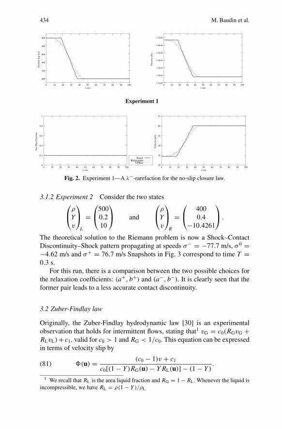
3.1.1 Experiment 1 Consider the left (L) and right (R) states

ρ

Y

v

L

=

5000.2

34.4233

and

ρ

Y

v

R

=

4000.250

.

These have been tailored so that the solution to the Riemann problem is apure λ−-rarefaction. With aG = 100 m/s, the speeds of propagation of thefronts are λ−

L = −40.12 m/s and λ−R = −15.77 m/s. Snapshots in Fig. 2

correspond to time T = 0.8 s.


Experiment 1

80 9050 7060

1.2e+6

1.1e+6

x (m)

Vel

ocity

(m

/s)

100

35

55

50

45

40

0 40302010

VFRoe

80706050 90

Relaxation

x (m)

Pres

sure

(Pa

)

10040

1.6e+6

1.5e+6

1.4e+6

1.3e+6

1.7e+6

3020100

400

70605040 80x (m)

Den

sity

(kg

/ m3)

1009030

460

440

420

Exact

480

20100

500

080706050 90

30

x (m)

Gas

Mas

s Fr

actio

n

10040

0.8

0.6

0.4

0.2

1

3020100

Fig. 2. Experiment 1—A λ−-rarefaction for the no-slip closure law.

3.1.2 Experiment 2 Consider the two states

ρ

Y

v

L

=

5000.210

and

ρ

Y

v

R

=

4000.4

−10.4261

.

The theoretical solution to the Riemann problem is now a Shock–ContactDiscontinuity–Shock pattern propagating at speeds σ− = −77.7 m/s, σ 0 =−4.62 m/s and σ+ = 76.7 m/s Snapshots in Fig. 3 correspond to time T =0.3 s.

For this run, there is a comparison between the two possible choices forthe relaxation coefficients: (a+, b+) and (a−, b−). It is clearly seen that theformer pair leads to a less accurate contact discontinuity.

3.2 Zuber-Findlay law

Originally, the Zuber-Findlay hydrodynamic law [30] is an experimentalobservation that holds for intermittent flows, stating that1 vG = c0(RGvG +RLvL)+ c1, valid for c0 > 1 and RG < 1/c0. This equation can be expressedin terms of velocity slip by

(u) = (c0 − 1)v + c1

c0[(1 − Y )RG(u) − YRL(u)] − (1 − Y ).(81)

1 We recall that RL is the area liquid fraction and RG = 1 − RL. Whenever the liquid isincompressible, we have RL = ρ(1 − Y )/ρL


Experiment 2

6030 5040

Pres

sure

(Pa

)

100908070

70 90806050 100

20100

x (m)

Gas

Mas

s Fr

actio

n

0 30 40 50 6020

5

10

15

10 70

−5

−10

−15

x (m)

0

80 90 100

Vel

ocity

(m

/s)

x (m)

1.6e+6

0.45

0.40

0.35

0.30

Exact

450

400

(a+,b+)(a−,b−)

0.25

2.0e+6

1.9e+6

1.8e+6

1.7e+6

2.1e+6

0.20

0.15

2.4e+6

2.3e+6

2.2e+6

500

x (m)

Den

sity

(kg

/ m3)

10090

0 40302010

80100

600

550

20 7060504030

Fig. 3. Experiment 2—A 3-wave Riemann problem for the no-slip closure law.

The Zuber-Findlay law has been extensively studied by Benzoni-Gavage[3] in her thesis. Benzoni succeeded in constructing solutions to some Rie-mann problems involving this law. Inspired from this work, we consider

ρ

Y

v

L

=

453.1970.0070524.8074

and

ρ

Y

v

R

=

454.9150.01081.7461

.

The other parameters are: aG = 300 m/s, c0 = 1.07, c1 = 0.2162 m/s. Thesolution has the pattern Shock–Contact Discontinuity–Shock propagating atspeeds σ− = −40.03 m/s, σ 0 = 10 m/s and σ+ = 67.24 m/s. Snapshots inFig. 4 correspond to time T = 0.5 s.

3.3 Dispersed law

We now use an hydrodynamic law

(u) = −δ/RL(u)(82)

that holds for two-phase flows with little bubbles of gas. Here, δ = 1.534√

gσ/ρL sin θ and σ = 7.5.10−5 is the superficial stress. Inspired from thework of Benzoni-Gavage [3], we consider

ρ

Y

v

L

=

901.11

1.2330.10−3

0.95027

and

ρ

Y

v

R

=

208.88

4.2552.10−2

0.78548

.


Experiment 3

50 6020 4030

Vel

ocity

(m

/s)

100908070

x (m)

15

10

5

0

20

100

30

25

0.5e+6

80706050 900.4e+6

x (m)

Den

sity

(kg

/ m3)

10040

550

500

450

x (m)

600

3020100

Exact

40302010 50 908070600

0.007

0.006VFRoe

Relaxation

0.008

0.012

0.011

0.01

0.009

100

60504030 70

Pres

sure

(Pa

)

100908020

0.7e+6

0.6e+6

x (m)

Gas

Mas

s Fr

actio

n

0.8e+6

100

1.1e+6

1.0e+6

0.9e+6

Fig. 4. Experiment 3—A 3-wave Riemann problem for the Zuber-Findlay law

The other parameters are: aG = 300 m/s, θ = π2 and g = 9.81 m/s2.

The solution is a Contact Discontinuity propagating at speed σ = 1 m/s.Snapshots in Fig. 5 correspond to time T = 20 s.

Experiment 4

100

Den

sity

(kg

/ m3)

x (m)100 605040302010 30200

1000

40 9080706050

Pres

sure

(Pa

)

10 20 30 400

80 90 100x (m)

50x (m)

VFRoeRelaxation

70

Vel

ocity

(m

/s)

60 70 80 90 100

0.90e+6

0.80

0.75

0.045

0.040

0.85

Exact

1.00

0.95

0.90

0.035

1.10e+6

1.05e+6

1.00e+6

0.95e+6

0.005

0.030

0.025

0.020

0.015

0.010

0

300

200

x (m)

Gas

Mas

s Fr

actio

n

400

900

800

700

600

500

1003020100 40 9080706050

Fig. 5. Experiment 4—Contact Discontinuity for the dispersed law


3.4 Synthetic law

When dealing with industrial cases, we must use a hydrodynamic law whichcan handle all types of flows: stratified, intermittent (the Zuber-Findlay law),dispersed, etc... However, each slip-law (u) is only valid for certain val-ues of u. In practice, physicists draw maps which describes the subsets ofthe admissible space in which a determined slip-law is valid. It happens thatfrom one subset to another subset, the slip-law is non-continuous! An attempthas been made to design a continuous slip-law (u) that is able to representvarious flow regimes. We call it the “synthetic law”. Here, we will use thevariable w = L(u) = (RG, p, us) where us = RLvL+RGvG is the superficialvelocity. The function L is a non-linear operator which will not be detailedhere. We will describe in the next paragraph how we design the function(w), from which we can recover the slip function (u) by the change ofvariable (u) = M((w), w) with w = L(u). Again, the non-linear oper-ator M will not be detailed here. We assume that there are just 3 types offlows: the dispersed flow with 0 ≤ RG < 1/3, the Zuber-Findlay flow with1/3 ≤ RG < 2/3 and the stratified flow with 2/3 ≤ RG ≤ 1. We then writethe slip law under the form:

UG = (w) = us0(RG, p) + 1(RG, p)(83)

where UG = RGvG. The function 0 and 1 are then computed by polyno-mial interpolation in order to ensure the continuity of , the validity of thelaw on the different ranges and compatibility conditions.

The previous lines show that the function (u) is highly non-linear. In thiscase, the solution of the Riemann problem is only composed of shocks sinceall the fields are really non-linear. No analytical solution is known at this datefor this slip-law. However, we can compute states which are connected by thetwo Rankine-Hugoniot conditions [v]2+[P ][τ ] = 0 and [v][Y ]−[σ ][τ ] = 0,which are solved by a non-linear solver. The two states

ρ

Y

v

L

=

492.7

0.20763−50.331

and

ρ

Y

v

R

=

400.

0.2−65.65

satisfy these conditions. The eigenvalues of the Jacobian matrices are λL =(−124.9, −55.0, 26.0) and λR = (−132.0, −73.6, 2.4). The speed ofthe discontinuity is s = 15.766 (m/s). Therefore, the Lax entropy conditionshows that the exact solution is a 3-shock since λ3

L = 26.0 > s > λ3R = 2.4.

The other parameters are: aG = 100 m/s and θ = 0. Snapshots in Fig. 6correspond to time T = 2 s.


Experiment 5

908060 7050

−64

−62

−66

x (m)

Pres

sure

(Pa

)

10090

Den

sity

(kg

/ m3)

1008070x (m)

403020100

Vel

ocity

(m

/s)

80706050

0.200

90 100x (m)

VFRoeRelaxation

40

−54

−56

−58

−60

−52

3020100

−50

1.1e+6

0.207

0.206

0.205

0.204

0.208

3020100

0.209

0.203

1.5e+6

1.4e+6

1.3e+6

1.2e+6

1.6e+6

0.202

0.201

0.199

Exact

1.7e+6

40

0

500

480

460

10 6050403020

440

80706050 90

420

400

x (m)

Gas

Mas

s Fr

actio

n

100

Fig. 6. Experiment 5—3-shock for the synthetic law

Conclusion

In view of the numerical results, this first attempt to solve a simplified two-phase flow system by a relaxation method can be considered as successful.This is all the more astonishing that, at first sight, the relaxation proceduremay seem “brute”, in comparison with the usual relaxation strategies for otherproblems [6].

The next steps are: incorporation of source terms, second-order schemesand boundary conditions. One important step will be the extension of thisexplicit scheme to an linearly implicit scheme, in order to get rid of the CFLtime step limitation. Variable sections and multicomponent flows can also beenvisaged.

Acknowledgements. The authors are greatly indebted to C. Chalons, E. Duret, P. Hochand V. Martin for their help in the preparation of the present work and to the InstitutFrancais du Petrole for its financial support. We are also grateful to I. Faille and F. Willienfor the numerous helpful discussions we had. Finally, we wish to thank the CEMRACS’99for having initiated this research project [6].

References

1. Aregba-Driollet, D., Natalini, R.: Convergence of relaxation schemes for conservationlaws. Appl. Anal. 1996, pp. 163–190


2. Baer, M.R., Nunziato, J.W.: A two-phase mixture theory for the deflagration-to-deto-nation transition in reactive granular materials. Int. J. Multiphase Flow, 12, 861–889(1986)

3. Benzoni-Gavage, S.: Analyse Numerique des Modeles Hydrodynamiques d’Ecoule-ments Diphasiques Instationnaires dans les Reseaux de Production Peroliere. Thesede Doctorat, Ecole Normale Superieure de Lyon, 1991

4. Bouchut, F.: Entropy satisfying flux vector splittings and kinetic BGK models. Pre-print, 2000

5. Chen, G., Levermore, C., Liu, T.: Hyperbolic conservation laws with stiff relaxationterms and entropy. Commun. Pure Appl. Math. 1995, pp. 787–830

6. Coquel, F., Cordier, S.: Le Centre d’ete de Mathematiques et de Recherches Avanceesen Calcul Scientifique 1999. Matapli, 62, 2000

7. Coquel, F., Godlewski, E., In, A., Perthame, B., Rascle, P.: Some new Godunov andrelaxation methods for two-phase flows. In: Procedings of and International confer-ence on Godunov methods: Theory and Applications, E. Toro, (ed.), Kluwer Aca-demic/Plenum Publishers, December, 2001

8. Coquel, F., Perthame, B.: Relaxation of energy and approximate Riemann solversfor general pressures laws in fluid dynamics. SIAM J. Numer. Math. 35, 2223–2249(1998)

9. Despres, B.: Invariance properties of Lagrangian systems of conservation laws,approximate Riemann solvers and the entropy condition. To appear in Numer. Math.,2002

10. Faille, I., Heintze, E.: A rough finite volume scheme for modeling two phase flow ina pipeline. Computers and Fluids 28, 213–241 (1999)

11. Gallouet, T., Masella, J.-M.: A rough Godunov scheme. In: C. R. Acad. Sci. Paris,1996, pp. 77

12. Godlewski, E., Raviart, P.-A.: Numerical approximation of hyperbolic systems ofconservation laws. Applied Mathematical Sciences, Springer, 1995

13. Harten,A., Lax, P., van Leer, B.: On upstream differencing and godunov-type schemesfor hyperbolic conservation laws. SIAM Review, 1983, pp. 35–61

14. Jin, S., Slemrod, M.: Regularization of the Burnett equations for rapid granular flowsvia relaxation. Physica D 150, 207–218 (2001)

15. Jin, S., Slemrod, M.: Regularization of the Burnett equations via relaxation. J. Stat.Phys. 103, 1009–1033 (2001)

16. Larrouturou, B.: How to preserve the mass fractions positivity when computing com-pressible multi-components flows. Tech. rep. INRIA, 1989

17. Lax, P.: Shock waves and entropy. In: Contributions to nonlinear functional analysis,Academic Press, New-York, 1971, pp. 603–634

18. Liu, T.: Hyperbolic conservation laws with relaxation. Commun. Math. Phys. 1987,pp. 153–175

19. Masella, J.-M., Tran, Q.-H., Ferre, D., Pauchon, C.: Transient simulation of two phaseflows in pipes. Int. J. Multiphase Flow 24, 739–755 (1998)

20. Natalini, R.: Convergence to equilibrium for the relaxation approximation of conser-vation laws. Commun. Pure Appl. Math. 1996, 1–30

21. Pauchon, C., Dhulesia, H., Binh-Cirlot, G., Fabre, J.: Tacite: a transient tool for mul-tiphase pipeline and well simulation. In: SPE annual Technical Conference, NewOrleans, 1994

22. Roe, P.: Approximate Riemann solver, parameter vectors and difference schemes.J. Comput. Phys., 1981, pp. 357–372

23. Saurel, R., LeMetayer, O.:A multiphase model for compressible flows with interfaces,shocks, detonation waves and cavitation. J. Fluid Mech. 431, 239–271 (2001)


24. Serre, D.: Systemes de lois de conservation I & II. Diderot editeur, 199625. Stewart, H.B., Wendroff, B.: Two-phase flow: Models and methods. J. Comput. Phys.

56, 363–409 (1984)26. Suliciu, I.: Energy estimates in rate-type thermo-viscoplasticity. Int. J. Plast., 1998,

pp. 227–24427. Wagner, D.H.: Equivalence of the Euler and Lagrangian equations of gas dynamics

for weak solutions. J. Diff. Equations 68, 118–136 (1987)28. Whitham, J.: Linear and Nonlinear Waves. New-York, 197429. Xin, Z., Jin, S.: The relaxation schemes for systems of conservation laws in arbitrary

space dimensions. Commun. Pure Appl. Math. 48, 235–276 (1995)30. Zuber, N., Findlay, J.: Average volumetric concentration in two-phase flow systems.

J. Heat Transfer, C87, 453–458 (1965)

A relaxation method for two-phase flow models with hydrodynamic closure law

Documents

Transcript of A relaxation method for two-phase flow models with hydrodynamic closure law