faculty of science and engineering

mathematics and applied mathematics

A Realistic Simulation of a Waterlens using Comflow

Bachelor’s Project Mathematics

August 2021

Student: S. Sulkers

First supervisor: Dr. ir. R. Luppes

Second assessor: Dr. A.E. Sterk

Abstract

The worldwide demand for energy grows and so does the need for reusable energy. Methodsusing water to generate electricity, such as hydroelectricity, are a clean alternative to othermethods. A water turbine needs a height difference of water to work properly and thereforeis not always feasible in the Netherlands due to the flat landscape. A waterlens is a way ofovercoming this problem by creating the height difference from a smaller wave. The waterlenscan create this height difference by letting small waves flow through a narrowing channel.The water will be ‘caught’ in a tank and stored until it is used to generate energy. In thisstudy the effects of different narrowing channels are observed and compared to each other.Simulations are made in ComFLOW in 3 dimensions. In the simulations different ratios andshapes of the narrowing channel are observed and the optimal ratio and shape is determined.The narrowest channel seems the most effective. Different waves can have different impacts,so a 2nd order Stokes wave will be compared to a 5th order Stokes wave. Once the optimalchannel is determined, the optimal point to ‘catch’ the water will be determined for thisoptimal channel. It seems that this point is near the end of the channel.

2

Contents

1 Introduction 4

2 Comflow 5

3 Research questions 7

4 Setup of the reference channel 84.1 Refining of the grid . . . . . . . . . . . . . . . . . . . . . . . . . . . . . . . . . . . . 9

5 Comparing various channels 115.1 Monitor points . . . . . . . . . . . . . . . . . . . . . . . . . . . . . . . . . . . . . . 115.2 Different ratios . . . . . . . . . . . . . . . . . . . . . . . . . . . . . . . . . . . . . . 11

5.2.1 Different lengths . . . . . . . . . . . . . . . . . . . . . . . . . . . . . . . . . 115.2.2 Different narrowness . . . . . . . . . . . . . . . . . . . . . . . . . . . . . . . 13

5.3 Different shapes . . . . . . . . . . . . . . . . . . . . . . . . . . . . . . . . . . . . . . 145.4 Different waves . . . . . . . . . . . . . . . . . . . . . . . . . . . . . . . . . . . . . . 17

6 Optimal placement of the water tank 196.1 Monitor Boxes . . . . . . . . . . . . . . . . . . . . . . . . . . . . . . . . . . . . . . 19

7 Conclusion 20

8 Discussion 21

Appendices 22

A Comflow code 22

3

1 Introduction

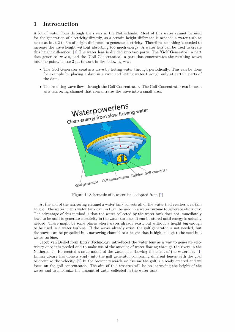
A lot of water flows through the rivers in the Netherlands. Most of this water cannot be usedfor the generation of electricity directly, as a certain height difference is needed: a water turbineneeds at least 2 to 3m of height difference to generate electricity. Therefore something is needed toincrease the wave height without absorbing too much energy. A water lens can be used to createthis height difference. [1] The water lens is divided into two parts: The ’Golf Generator’, a partthat generates waves, and the ’Golf Concentrator’, a part that concentrates the resulting wavesinto one point. These 2 parts work in the following way:

• The Golf Generator creates a wave by letting water through periodically. This can be donefor example by placing a dam in a river and letting water through only at certain parts ofthe dam.

• The resulting wave flows through the Golf Concentrator. The Golf Concentrator can be seenas a narrowing channel that concentrates the wave into a small area.

Figure 1: Schematic of a water lens adopted from [1]

At the end of the narrowing channel a water tank collects all of the water that reaches a certainheight. The water in this water tank can, in turn, be used in a water turbine to generate electricity.The advantage of this method is that the water collected by the water tank does not immediatelyhave to be used to generate electricity in the water turbine. It can be stored until energy is actuallyneeded. There might be some places where waves already exist, but without a height big enoughto be used in a water turbine. If the waves already exist, the golf generator is not needed, butthe waves can be propelled in a narrowing channel to a height that is high enough to be used in awater turbine.

Jacob van Berkel from Entry Technology introduced the water lens as a way to generate elec-tricity once it is needed and to make use of the amount of water flowing through the rivers in theNetherlands. He created a scale model of the water lens showing the effect of the waterlens. [1]Emma Cleary has done a study into the golf generator comparing different lenses with the goalto optimize the velocity. [2] In the present research we assume the golf is already created and wefocus on the golf concentrator. The aim of this research will be on increasing the height of thewaves and to maximize the amount of water collected in the water tank.

4

2 Comflow

The increase of wave heights by the application of a water lens will be studied using Comflow.Comflow is a program for numerical simulations of fluid flow. The simulations are based on theNavier-Stokes equations. Originally the Comflow software is created by the University of Groningento study sloshing of liquid fuel in space crafts. The program has been developed further, includingthe application of waves, which will be used in the simulations in this thesis. [3] The Navier-Stokesequations describe the motion of a fluid. Since all of the simulations in this thesis are done withwater, which is an incompressible and Newtonian fluid, the Navier-Stokes equations are given by:

Conservation of mass: ∇·−→u = 0

Conservation of momentum: ρD−→uDt

= −∇p+ µ∇2−→u + ρ−→g

In these equations, −→u is the velocity vector in 3 dimensions, p is the pressure, µ is the dynamicviscosity, ρ is the density and −→g the gravitational acceleration.

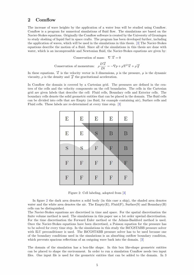
In Comflow the domain is covered by a Cartesian grid. The pressures are defined in the cen-tres of the cells and the velocity components on the cell boundaries. The cells in the Cartesiangrid are given labels that describe the cell: Fluid cells, Boundary cells and Exterior cells. Theboundary cells denote the solid geometric entities that can be placed in the domain. The fluid cellscan be divided into cells that are Empty (no fluid, for example containing air), Surface cells andFluid cells. These labels are re-determined at every time step. [3]

Figure 2: Cell labeling, adopted from [3]

In figure 2 the dark area denotes a solid body (in this case a ship), the shaded area denoteswater and the white area denotes the air. The Empty(E), Fluid(F), Surface(S) and Boundary(B)cells can be distinguished.The Navier-Stokes equations are discretised in time and space. For the spatial discretisation thefinite volume method is used. The simulations in this paper use a 1st order upwind discretisation.For the time discretisation the Forward Euler method or the Adams-Bashford method is used.Once the Navier-Stokes equations have been discretised, a Poisson equation for the pressure hasto be solved for every time step. In the simulations in this study the BiCGSTABB pressure solverwith ILU preconditioner is used. The BiCGSTABB pressure solver has to be used because oneof the boundary conditions used in the simulations is an absorbing outflow boundary condition,which prevents spacious reflections of an outgoing wave back into the domain. [3]

The domain of the simulation has a box-like shape. In this box like-shape geometric entitiescan be placed to shape the environment. In order to run a simulation Comflow needs two inputfiles. One input file is used for the geometric entities that can be added to the domain. In 3

5

dimensions 5 different geometric entities can be placed: a tetrahedon, wedge, brick, ellipsoid and(elliptic) cylinder. These geometric identities can be defined as solid structures or parts that areopen for the flow of a liquid. The other input file contains all of the data needed for the simulation:such as the definition of the domain; the boundary conditions at the in- and outflow; parametersfor the solvers; initial liquid configuration; the wave configuration; boundary conditions; informa-tion on which data to store; information about the placement of monitor points and when to takesnapshots. [3]

6

3 Research questions

A higher wave may have a much bigger energy yield due to the bigger potential energy the waterpossesses. Therefore it is important to investigate what the impact of a narrowing channel is onthe increase of the wave heights. There are a lot of different factors that might influence the waveheight.

As a start let a simple narrowing channel be defined. The first step is to change the propor-tions of the channel and measure the resulting impact on the wave height. The proportions canbe changed in different ways: both the narrowness and the length of the channel might impact thewave height. In the first set of simulations the length of the narrowing channel is changed and theeffect on the wave is compared. These simulations will be covered in section 5.2.1. In the secondset of simulations the narrowness of the channel is changed and compared. These simulations willbe covered in section 5.2.2.The expectation is that the length of a channel has no effect on the height of the wave. Onlythe length of the channel changes, not the narrowness. On the other hand it is expected that thenarrower a channel becomes, the higher the wave becomes. The wave in the narrower channel hasless space to occupy over time. As the channel becomes narrower the water is pushed through atinier space. The ’excess’ water then has to go up.It is also important to measure how much the wave increases compared to a straight channel. Ifthe increase is only marginal, there is no reason to make the channel any narrower. But in caseof a considerable increase of the wave height, say twice as much, the narrow channel would have asignificant impact on the wave height.

Not only the proportions might influence the wave height, also the shape of the channel couldhave an impact. Therefore the effect of a different shape on the height of the wave is also inves-tigated. An increasingly or decreasingly narrowing channel could have a different effect on theadditional wave height than a consistently narrowing channel. It is expected that an increasinglynarrowing channel results in lower wave height along the beginning of the channel, but overtakesthe height of the waves of the other channels towards the end of the channel. For the decreasinglynarrowing channel the opposite is expected: at the beginning of the channel the decreasingly nar-rowing channel is expected to have a higher wave than the other channels, but towards the endthe wave height will be lower or equal. Both an increasingly narrowing channel and a decreasinglynarrowing channel are compared with a consistently narrowing channel and a straight channel.These simulations will be covered in section 5.3.

There is a large variety regarding wave types and a different wave might behave differently when itflows through a narrowing channel. Realistically we want all waves to behave more or less the sameway, as the channel would not be practical in usage if only one type of wave can become higher.This can be simulated by taking one simple narrowing channel and observe what happens whenthe type of wave is changed. The behaviour of these two different types of wave will be comparedto each other. The simulations will be covered in section 5.4.

The goal of the water lens is to increase the netto gain of energy generated by the water tur-bine. The more water is used in the water turbine, the more power can be generated. The waterturbine can only use water up from a certain height. It is useful to ask how much water can becollected from a certain height on. Therefore it is important to determine the most optimal placein the narrowing channel to collect the water. The most optimal place to collect the water will bedetermined in section 6.

All of these concepts lead to the following research questions:

• What is the effect of different ratios of the narrowing channels?

• What is the effect of different shapes of the narrowing channels?

• What is the effect of different waves?

• What is the optimal place to catch the water?

7

4 Setup of the reference channel

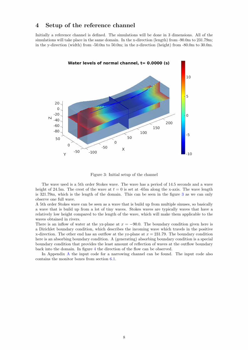
Initially a reference channel is defined. The simulations will be done in 3 dimensions. All of thesimulations will take place in the same domain. In the x-direction (length) from -90.0m to 231.79m;in the y-direction (width) from -50.0m to 50.0m; in the z-direction (height) from -80.0m to 30.0m.

Figure 3: Initial setup of the channel

The wave used is a 5th order Stokes wave. The wave has a period of 14.5 seconds and a waveheight of 24.5m. The crest of the wave at t = 0 is set at -65m along the x-axis. The wave lengthis 321.79m, which is the length of the domain. This can be seen in the figure 3 as we can onlyobserve one full wave.A 5th order Stokes wave can be seen as a wave that is build up from multiple sinuses, so basicallya wave that is build up from a lot of tiny waves. Stokes waves are typically waves that have arelatively low height compared to the length of the wave, which will make them applicable to thewaves obtained in rivers.There is an inflow of water at the yz-plane at x = −90.0. The boundary condition given here isa Dirichlet boundary condition, which describes the incoming wave which travels in the positivex-direction. The other end has an outflow at the yz-plane at x = 231.79. The boundary conditionhere is an absorbing boundary condition. A (generating) absorbing boundary condition is a specialboundary condition that provides the least amount of reflection of waves at the outflow boundaryback into the domain. In figure 4 the direction of the flow can be observed.

In Appendix A the input code for a narrowing channel can be found. The input code alsocontains the monitor boxes from section 6.1.

8

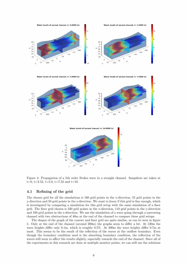
Figure 4: Propagation of a 5th order Stokes wave in a straight channel. Snapshots are taken att=0, t=2.52, t=5.0, t=7.52 and t=10.

4.1 Refining of the grid

The chosen grid for all the simulations is 160 grid points in the x-direction, 55 grid points in they-direction and 50 grid points in the z-direction. We want to know if this grid is fine enough, whichis investigated by comparing a simulation for this grid setup with the same simulation of a finergrid. The finer grid chosen is 320 grid points in the x-direction, 110 grid points in the y-directionand 100 grid points in the z-direction. We use the simulation of a wave going through a narrowingchannel with two obstructions of 40m at the end of the channel to compare these grid setups.

The shapes of the graph of the coarser and finer grid are quite similar, as can be seen in figure5. Only at the end of the channel (around 200m) the graphs seem to differ a bit. At 120m thewave heights differ only 0.1m, which is roughly 0.5%. At 200m the wave heights differ 0.7m atmost. This seems to be the result of the reflection of the waves at the outflow boundary. Eventhough the boundary condition used is the absorbing boundary condition, the reflection of thewaves still seem to affect the results slightly, especially towards the end of the channel. Since all ofthe experiments in this research are done at multiple monitor points, we can still use the solutions

9

at the end of the channel. However, it is important to keep in mind that the solutions towards theend of the channel are less accurate.

Figure 5: Grid comparison of the finer and coarser grid at 40m, 80m, 120m, 160m and 200m.

10

5 Comparing various channels

5.1 Monitor points

In these different simulations the height of the wave has to be measured somehow and comparedto the height of the wave in other channels. In the simulations monitor points are used to measurethe height of a wave over time. These monitor points measure the wave height at certain locationsin the domain. All of these locations are centered in the middle of the channel (y=0m). In thex-direction 5 different monitor points are distinguished: at 40m, 80m, 120m, 160m and 200mmeasured from the start of the narrowing part of the channel. The monitor points can be observedin figure 6. The dark blue rods denote the monitor points.

Figure 6: Monitor points are positioned at 40m, 80m, 120m, 160m and 200m on the centerline(y=0m).

5.2 Different ratios

In sections 5.2.1 and 5.2.2 narrowing channels with different ratios are simulated and the waterheight of these narrowing channels are compared to each other. All of these narrowing channelsare built in the same way: two wedges are placed in the reference channel discussed in section 4.These two wedges are placed in such a way that the channel becomes narrower towards the end.In figure 7 we see an example of a narrowing channel with a length of 200m and a width of 40mper wedge.

5.2.1 Different lengths

For the first set of simulations the length of the narrowing channel is changed. The lengths of thenarrowing channels are 40m, 120m and 200m. The height of the wave is measured immediatelyat the end of the narrowing channel. All narrowing channels have the same wave configuration,which is the same as in section 4. The width of the wedges in the narrowing channels is 40m. Infigure 8 the wave height of the channels is plotted against the time.

The 3 waves seem to have the same shape and approximately have the same maximum height.The monitor points are taken at the end of each channel. This means that for the channel withlength 40m the wave is measured at 40m after the channel becomes narrower. The shift in timecan be explained by the fact that the waves are monitored at the end of each channel.

11

Figure 7: Setup of a narrowing channel using wedges

Figure 8: Wave height comparison of narrowing channels varying in length

12

5.2.2 Different narrowness

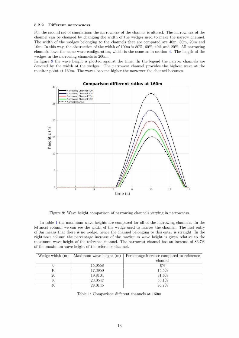
For the second set of simulations the narrowness of the channel is altered. The narrowness of thechannel can be changed by changing the width of the wedges used to make the narrow channel.The width of the wedges belonging to the channels that are compared are 40m, 30m, 20m and10m. In this way, the obstruction of the width of 100m is 80%, 60%, 40% and 20%. All narrowingchannels have the same wave configuration, which is the same as in section 4. The length of thewedges in the narrowing channels is 200m.In figure 9 the wave height is plotted against the time. In the legend the narrow channels aredenoted by the width of the wedges. The narrowest channel provides the highest wave at themonitor point at 160m. The waves become higher the narrower the channel becomes.

Figure 9: Wave height comparison of narrowing channels varying in narrowness.

In table 1 the maximum wave heights are compared for all of the narrowing channels. In theleftmost column we can see the width of the wedge used to narrow the channel. The first entryof 0m means that there is no wedge, hence the channel belonging to this entry is straight. In therightmost column the percentage increase of the maximum wave height is given relative to themaximum wave height of the reference channel. The narrowest channel has an increase of 86.7%of the maximum wave height of the reference channel.

Wedge width (m) Maximum wave height (m) Percentage increase compared to referencechannel

0 15.0558 0%10 17.3950 15.5%20 19.8104 31.6%30 23.0547 53.1%40 28.0145 86.7%

Table 1: Comparison different channels at 160m.

13

5.3 Different shapes

The narrowest channel from section 5.2 is compared to different shapes of the obstruction. Insteadof a constantly narrowing channel an increasingly and decreasingly narrowing channel are created.These channels are made in the same way the earlier narrowing channels are made but with differentcurved shapes.

The concave channel is made by first defining a solid brick structure. An elliptic cylinderis subsequently used to cut out a part of the brick. This elliptic cylinder is defined as a liquidstructure, so water can flow through this part. The resulting channel has a concave shape asindicated in figure 10.

Figure 10: A concave lens

The convex channel is made by defining two solid elliptic cylinders. The middle point of the

cylinder is placed at the edges of the domain at the end of the x-axis. In this way only1

4of the

elliptic cylinder is placed on the domain. The resulting channel has a convex shape as indicatedin figure 11.

Figure 11: A convex lens

14

The simulations are done with the same wave configuration as in section 4. The same monitorpoints at 40m, 80m, 120m, 160m and 200m are used to determine the wave height of the narrowingchannels. The wave height of the convex, concave, constantly narrowing and normal channel atthese locations are plotted in figure 12.

Figure 12: Wave height comparison of the convex, concave, straight narrowing and normal channelat 40m, 80m, 120m, 160m and 200m.

From figure 12 it is observed that the convex channel immediately has the highest wave at thebeginning of the channel, as expected. We also see that the concave channel has the lowest waveat the start, as expected. The convex channel keeps having the highest wave at all of the monitorpoints, with exception of the monitor point at 160m, as can be seen in figure 13. The wave ofthe concave channel seems to increase a lot towards the end of the channel as in the first threemonitor points it stays quite close to the normal channel. The convex channel does seem to havethe highest wave compared to the other channels, which might be due to the amount of space this

15

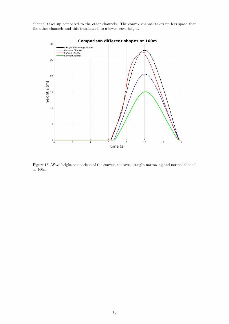
channel takes up compared to the other channels. The convex channel takes up less space thanthe other channels and this translates into a lower wave height.

Figure 13: Wave height comparison of the convex, concave, straight narrowing and normal channelat 160m.

16

5.4 Different waves

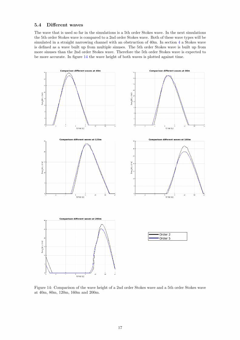
The wave that is used so far in the simulations is a 5th order Stokes wave. In the next simulationsthe 5th order Stokes wave is compared to a 2nd order Stokes wave. Both of these wave types will besimulated in a straight narrowing channel with an obstruction of 40m. In section 4 a Stokes waveis defined as a wave built up from multiple sinuses. The 5th order Stokes wave is built up frommore sinuses than the 2nd order Stokes wave. Therefore the 5th order Stokes wave is expected tobe more accurate. In figure 14 the wave height of both waves is plotted against time.

Figure 14: Comparison of the wave height of a 2nd order Stokes wave and a 5th order Stokes waveat 40m, 80m, 120m, 160m and 200m.

17

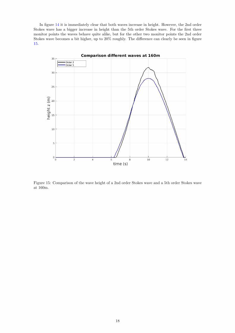
In figure 14 it is immediately clear that both waves increase in height. However, the 2nd orderStokes wave has a bigger increase in height than the 5th order Stokes wave. For the first threemonitor points the waves behave quite alike, but for the other two monitor points the 2nd orderStokes wave becomes a bit higher, up to 20% roughly. The difference can clearly be seen in figure15.

Figure 15: Comparison of the wave height of a 2nd order Stokes wave and a 5th order Stokes waveat 160m.

18

6 Optimal placement of the water tank

6.1 Monitor Boxes

The optimal place to collect water will be determined in a similar way as the wave height. Thewave height was measured at certain points in the domain using monitor points. Since the amountof water is measured in 3 dimensions we cannot use points, but have to use boxes. In figure 16 33monitor boxes are placed in the middle of the channel over the length of the channel:

Figure 16: Monitor boxes are placed every 5m at the centerline (y=0).

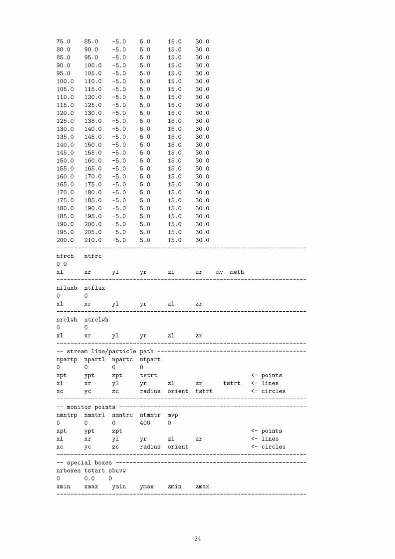
The boxes are 10m long, 10m wide and 15m high. The boxes are placed in the middle of thechannel, ranging from 40m-200m in the x-direction, from -5m to 5m in the y-direction and from15m to 30m in the z-direction. Every 5m a box is placed. This means that the boxes in figure 16are overlapping each other. The amount of liquid passing through these boxes is plotted againsttime in figure 17.

The boxes in figure 17 are distinguished by the placement of the x-axis. The first box is placedfrom 55m-65m. Not all monitor boxes are taken, since it would be too chaotic to read anything.The highest fill rate seems to be obtained in the box placed at 155m-165m. This means that inthis case the optimal place to put the water turbine would be near the end of the channel, butbefore the end of the channel.

19

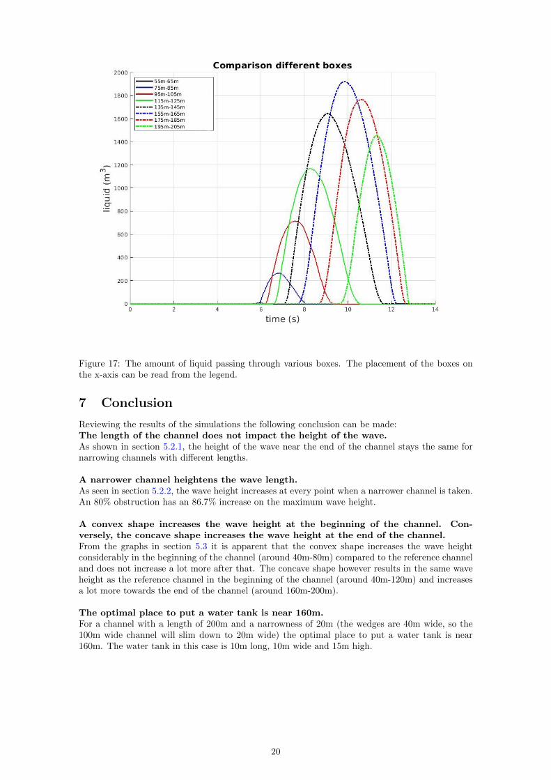
Figure 17: The amount of liquid passing through various boxes. The placement of the boxes onthe x-axis can be read from the legend.

7 Conclusion

Reviewing the results of the simulations the following conclusion can be made:The length of the channel does not impact the height of the wave.As shown in section 5.2.1, the height of the wave near the end of the channel stays the same fornarrowing channels with different lengths.

A narrower channel heightens the wave length.As seen in section 5.2.2, the wave height increases at every point when a narrower channel is taken.An 80% obstruction has an 86.7% increase on the maximum wave height.

A convex shape increases the wave height at the beginning of the channel. Con-versely, the concave shape increases the wave height at the end of the channel.From the graphs in section 5.3 it is apparent that the convex shape increases the wave heightconsiderably in the beginning of the channel (around 40m-80m) compared to the reference channeland does not increase a lot more after that. The concave shape however results in the same waveheight as the reference channel in the beginning of the channel (around 40m-120m) and increasesa lot more towards the end of the channel (around 160m-200m).

The optimal place to put a water tank is near 160m.For a channel with a length of 200m and a narrowness of 20m (the wedges are 40m wide, so the100m wide channel will slim down to 20m wide) the optimal place to put a water tank is near160m. The water tank in this case is 10m long, 10m wide and 15m high.

20

8 Discussion

Some remarks have to be made regarding the numerical experiments conducted in this study.The simulations are done with only 2 types of waves: Stokes 5th order waves and Stokes 2nd orderwaves. In a more realistic simulation more different wave types have to be observed to concludesomething about the influence of the channel.

Since the time used to do simulations was only limited, the grid can only be refined up to acertain refinement. Every doubling of the grid would take 8 time as much time due to all of thesimulations taking place in a 3 dimensional domain. By increasing the number of monitor pointsand boxes the accuracy of the results can also be increased.

Even with the absorbing boundary conditions some disturbance occurs at the end of the chan-nel. This could be solved by taking a domain that has twice the length of the wave length, whilekeeping the channel at the same length. This would result in twice the amount of computationaltime needed to carry out the simulations.

In chapter 5.3 different shapes of the channel are compared to a straight channel. The Com-flow software only has a finite amount of shapes to use, thus limiting the options. However, evenwith this limited amount of shapes an infinite amount of channel configurations could be build.Only a couple of simple configurations were treated in this study. When considering shapes, a lotmore different and complex shapes can be studied.

One thing that also seems to influence the wave height is the volume the obstruction of a nar-rowing channel takes up. For example, the convex shape in section 5.3 took up more volume thanthe concave shape. Consequently the maximum wave height of the convex shape is higher than themaximum wave height of the concave shape at the end of the channel. For a next investigation theamount of volume the obstructions take up in the channel should be considered as a research topic.

The optimal place of a water tank was determined for one of the narrowing channels. A lotof factors come into play, which could be extended in another study. The height, length, widthand placement of the box all influence the amount that will be caught. But also the type of wave,type of channel, narrowness of the channel and shape of water tank will influence the water col-lected in this water tank. Next to that, also the influence of a water turbine under the water tankshas to be investigated.Nonetheless, the experiments conducted in this study are a good first step into the exploration ofthe effect of narrowing channels on wave height and hence on the application for water lenses forgenerating energy.

21

Appendices

A Comflow code

-- Title ---------------------------------------------------------------

Optimal placement water box

------------------------------------------------------------------------

slosh mvbd twph nproc

1 0 0 4

------------------------------------------------------------------------

-- domain definition ---------------------------------------------------

xmin xmax ymin ymax zmin zmax

-90.0 231.7889 -50.0 50.0 -80.0 30.0

------------------------------------------------------------------------

-- green water parameters ----------------------------------------------

grnwtr

0

------------------------------------------------------------------------

high low length

0.0 0.0 0.0

------------------------------------------------------------------------

width a b

0.0 0.0 0.0

------------------------------------------------------------------------

-- definition initial liquid configuration -----------------------------

liqcnf lqxmin lqxmax lqymin lqymax lqzmin lqzmax

1 0.0 1000.0 -30.0 30.0 -290.0 0.0

------------------------------------------------------------------------

-- definition of incoming wave -----------------------------------------

wave wvstart period wheight xcrest waterd ramp* order curr beta

5 1 14.5 24.3 -65.0 80.0 0 10 0.0 0.0

ramp val1 val2

0 0.0 0.0

------------------------------------------------------------------------

-- definition of in- and outflow boundaries ----------------------------

nrio

2

i/o plane xmin xmax ymin ymax zmin zmax

1 1 -90.0 -90.0 -50.0 50.0 -80.0 30.0

11 1 231.7889 231.7889 -50.0 50.0 -80.0 30.0

------------------------------------------------------------------------

-- partial slip --------------------------------------------------------

pscnf psl

0 0.0

------------------------------------------------------------------------

-- absorbing boundary condition ----------------------------------------

bcl bcr gabc a0 a1 b1 kh1 kh2~ alfa1 alfa2

1 1 1 1.05 0.12 0.31 1.345 5.0 0.0 0.0

------------------------------------------------------------------------

-- definition of numerical beach in positive x-direction ---------------

numbch dampto* slope bxstart

0 0 0.0 0.0

------------------------------------------------------------------------

-- physical parameters -------------------------------------------------

rho1 rho2 mu1 mu2 sigma theta patm gamma

1.0e3 1.0 1.0e-3 1.71e-5 0.0 90.0 1.0e5 1.4

------------------------------------------------------------------------

-- grid parameters -----------------------------------------------------

griddef

1

22

imax jmax kmax xc yc zc sx sy sz

160 55 50 25.0 0.0 12.26 1.0 1.0 1.0

------------------------------------------------------------------------

-- numerical parameters ------------------------------------------------

eps omega itmax alpha feab0 feab1 feab2 nrintp fslinext

1.0E-6 1.0 10000 1.0 0.0 1.0 0.0 3 1

------------------------------------------------------------------------

-- numerical parameters two-phase flow ---------------------------------

solver extrap restol imptol upwind imprel irhoav itscr

5 0 1.0E-7 1.0E-3 1 1.0 1 0

------------------------------------------------------------------------

-- time parameters/cfl number ------------------------------------------

dt tmax dtmax cfl cflmin cflmax divl

0.01 14.0 0.058 1 0.2 0.5 0

------------------------------------------------------------------------

-- free surface methods ------------------------------------------------

vofmth vofcor divl

1 2 0

------------------------------------------------------------------------

-- gravitation ---------------------------------------------------------

gravx gravy gravz ginrt finrt

0.0 0.0 -9.81 0 0

------------------------------------------------------------------------

-- motion of coordinate system -----------------------------------------

motionframe

0

amplx freqx amply freqy amplz freqz

0.0 0.0 0.0 0.0 0.0 0.0

------------------------------------------------------------------------

omex omey omez x0 y0 z0

0.0 0.0 0.0 0.0 0.0 0.0

------------------------------------------------------------------------

-- autosave ------------------------------------------------------------

load nsave

0 2

------------------------------------------------------------------------

-- post-processing: snapshots/screen print/center of mass --------------

npm2d npm3d compr nprnt ntcom

0 140 0 140 0

------------------------------------------------------------------------

npmslic nyz nxz nxy

0 0 0 0

planeyz

planexz

planexy

------------------------------------------------------------------------

-- directory name for snapshots ----------------------------------------

pathname snapshot data:

data/

------------------------------------------------------------------------

-- fill boxes, force boxes and flux boxes-------------------------------

nfillb ntfill

33 1400

xl xr yl yr zl zr

40.0 50.0 -5.0 5.0 15.0 30.0

45.0 45.0 -5.0 5.0 15.0 30.0

50.0 60.0 -5.0 5.0 15.0 30.0

55.0 65.0 -5.0 5.0 15.0 30.0

60.0 70.0 -5.0 5.0 15.0 30.0

65.0 75.0 -5.0 5.0 15.0 30.0

70.0 80.0 -5.0 5.0 15.0 30.0

23

75.0 85.0 -5.0 5.0 15.0 30.0

80.0 90.0 -5.0 5.0 15.0 30.0

85.0 95.0 -5.0 5.0 15.0 30.0

90.0 100.0 -5.0 5.0 15.0 30.0

95.0 105.0 -5.0 5.0 15.0 30.0

100.0 110.0 -5.0 5.0 15.0 30.0

105.0 115.0 -5.0 5.0 15.0 30.0

110.0 120.0 -5.0 5.0 15.0 30.0

115.0 125.0 -5.0 5.0 15.0 30.0

120.0 130.0 -5.0 5.0 15.0 30.0

125.0 135.0 -5.0 5.0 15.0 30.0

130.0 140.0 -5.0 5.0 15.0 30.0

135.0 145.0 -5.0 5.0 15.0 30.0

140.0 150.0 -5.0 5.0 15.0 30.0

145.0 155.0 -5.0 5.0 15.0 30.0

150.0 160.0 -5.0 5.0 15.0 30.0

155.0 165.0 -5.0 5.0 15.0 30.0

160.0 170.0 -5.0 5.0 15.0 30.0

165.0 175.0 -5.0 5.0 15.0 30.0

170.0 180.0 -5.0 5.0 15.0 30.0

175.0 185.0 -5.0 5.0 15.0 30.0

180.0 190.0 -5.0 5.0 15.0 30.0

185.0 195.0 -5.0 5.0 15.0 30.0

190.0 200.0 -5.0 5.0 15.0 30.0

195.0 205.0 -5.0 5.0 15.0 30.0

200.0 210.0 -5.0 5.0 15.0 30.0

------------------------------------------------------------------------

nfrcb ntfrc

0 0

xl xr yl yr zl zr mv meth

------------------------------------------------------------------------

nfluxb ntflux

0 0

xl xr yl yr zl zr

------------------------------------------------------------------------

nrelwh ntrelwh

0 0

xl xr yl yr zl zr

------------------------------------------------------------------------

-- stream line/particle path -------------------------------------------

npartp npartl npartc ntpart

0 0 0 0

xpt ypt zpt tstrt <- points

xl xr yl yr zl zr tstrt <- lines

xc yc zc radius orient tstrt <- circles

------------------------------------------------------------------------

-- monitor points ------------------------------------------------------

nmntrp nmntrl nmntrc ntmntr mvp

0 0 0 400 0

xpt ypt zpt <- points

xl xr yl yr zl zr <- lines

xc yc zc radius orient <- circles

------------------------------------------------------------------------

-- special boxes -------------------------------------------------------

nrboxes tstart sbuvw

0 0.0 0

xmin xmax ymin ymax zmin zmax

------------------------------------------------------------------------

24

References

[1] Entry Technology Support BV. https://web.tue.nl/cursor/bastiaan/jaargang48/

cursor29/achtergrond/oz_2.html.

[2] E.E. Cleary. A numerical study of water lenses using Comflow. University of Groningen, August2020.

[3] B. Iwanowski T. Bunnik B. Duz H. van der Heiden R. Wemmenhove P. Wellens A. Veldman T.Helmholt-Kleefsman E. Loots J. Helder R. Luppes, P. van der Plas. Manual Comflow Version3.9X/4.0. University of Groningen, November 2015.

25