Linköping University | Department of Physics, Chemistry and BiologyMaster’s Thesis, 30 hp | Applied Physics and Electrical Engineering

Spring term 2019 | LITH-IFM-A-EX--19/3636--SE

Propaga on of Radio Waves in aRealis c Environment using aParabolic Equa on Approach

Jonas Ehn

Examiner: Peter MüngerSupervisor: Tobias Hansson

External supervisor : Robert Jonsson

Avdelning, InstitutionDivision, Department

Division of Theoretical PhysicsDepartment of Physics, Chemistry and BiologyLinköping UniversitySE-581 83 Linköping, Sweden

DatumDate

2019-06-10

SpråkLanguage

Svenska/Swedish

Engelska/English

RapporttypReport category

Licentiatavhandling

Examensarbete

C-uppsats

D-uppsats

Övrig rapport

URL för elektronisk version

—

ISBN

—

ISRN

LITH-IFM-A-EX--19/3636--SE

Serietitel och serienummerTitle of series, numbering

ISSN

—

TitelTitle

Utbredning av radiovågor i en realistisk miljö genom paraboliska ekvationer

Propagation of RadioWaves in a Realistic Environment using a Parabolic Equation Approach

FörfattareAuthor

Jonas Ehn

SammanfattningAbstract

Radars are used for range estimation of distant objects. They operate on the principle ofsending electromagnetic pulses that are reflected off a target. This leads to the propagationof electromagnetic waves over large distances. As the waves propagate, they are affectedby several aspects that decrease the performance of the radar system. In this master thesis,we derive a mathematical model that describes electromagnetic propagation in the tropo-sphere. The model developed is based on a parabolic equation and uses the split-step Fouriermethod for its numerical solution. Using the model, we estimate the influence of a varying,complex, refractive index of the atmosphere, different lossy materials in the ground, terrain,and oceans. The terrain is described using a piecewise linear shift map method. The mod-elling of the ocean is done using a novel model which is a combination of terrain for largeswells and Miller surface roughness for smaller waves, both based on a Pierson-Moskowitzsea spectrum. The model is validated and found to agree very well, with results found in theliterature.

NyckelordKeywords Electromagnetic fields, wave propagation, radar, parabolic equation, split-step Fourier

method

To my friends and family

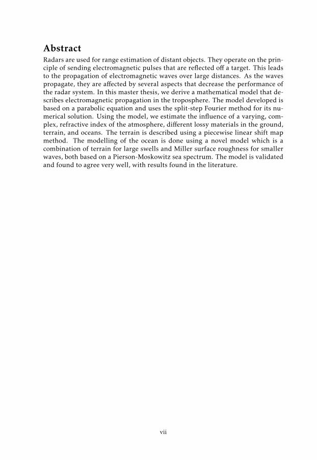
AbstractRadars are used for range estimation of distant objects. They operate on the prin-ciple of sending electromagnetic pulses that are reflected off a target. This leadsto the propagation of electromagnetic waves over large distances. As the wavespropagate, they are affected by several aspects that decrease the performance ofthe radar system. In this master thesis, we derive a mathematical model that de-scribes electromagnetic propagation in the troposphere. The model developed isbased on a parabolic equation and uses the split-step Fourier method for its nu-merical solution. Using the model, we estimate the influence of a varying, com-plex, refractive index of the atmosphere, different lossy materials in the ground,terrain, and oceans. The terrain is described using a piecewise linear shift mapmethod. The modelling of the ocean is done using a novel model which is acombination of terrain for large swells and Miller surface roughness for smallerwaves, both based on a Pierson-Moskowitz sea spectrum. The model is validatedand found to agree very well, with results found in the literature.

vii

AcknowledgementsFirst, I would like to thank my supervisor Robert Jonsson and Saab Dynamics forthe possibility to do this master’s thesis. Thank you, Robert, for all discussions,great advice and support over the course of these weeks. Your help has been in-dispensable. I would also like to thank the rest of the staff at Saab Dynamics thatI have come into contact with during this thesis. Thank you for being so patientwhen answering all my questions. I am also very grateful for all the thoughtfulfeedback that I have received from Tobias Hansson, my supervisor at the Depart-ment of Physics, Chemistry and Biology, both on the report and on numericalsimulation in general.

I would also like to thank Peter Holm at FOI for very inspiring discussions aboutpe-modelling. My understanding would have been greatly reduced without yourhelp.

This thesis marks the end of six years of studies in Linköping. I want to take thisopportunity to thank all my friends who have made these years an unforgettabletime. It is thanks to all of you that these years have been truly awesome.

Finally, I would like to thank my family for always supporting and believing inme. You have played a larger part in the making of this thesis than you know.

Linköping, June 2019Jonas Ehn

ix

Contents

Notation xiii

1 Introduction 11.1 Background . . . . . . . . . . . . . . . . . . . . . . . . . . . . . . . 11.2 Aim . . . . . . . . . . . . . . . . . . . . . . . . . . . . . . . . . . . . 21.3 Delimitations . . . . . . . . . . . . . . . . . . . . . . . . . . . . . . . 21.4 Layout . . . . . . . . . . . . . . . . . . . . . . . . . . . . . . . . . . 3

2 Theory 52.1 Radar . . . . . . . . . . . . . . . . . . . . . . . . . . . . . . . . . . . 52.2 Electromagnetic waves . . . . . . . . . . . . . . . . . . . . . . . . . 7

2.2.1 Em-propagation in vacuum . . . . . . . . . . . . . . . . . . 82.2.2 Em-propagation in lossy media . . . . . . . . . . . . . . . . 92.2.3 Boundary conditions . . . . . . . . . . . . . . . . . . . . . . 10

2.3 The parabolic equation . . . . . . . . . . . . . . . . . . . . . . . . . 122.3.1 Flat Earth . . . . . . . . . . . . . . . . . . . . . . . . . . . . 122.3.2 Round Earth . . . . . . . . . . . . . . . . . . . . . . . . . . . 14

2.4 The split-step Fourier method . . . . . . . . . . . . . . . . . . . . . 162.4.1 Method 1 . . . . . . . . . . . . . . . . . . . . . . . . . . . . . 162.4.2 Method 2 . . . . . . . . . . . . . . . . . . . . . . . . . . . . . 192.4.3 Sampling distance . . . . . . . . . . . . . . . . . . . . . . . . 232.4.4 Initial field . . . . . . . . . . . . . . . . . . . . . . . . . . . . 24

2.5 The atmosphere . . . . . . . . . . . . . . . . . . . . . . . . . . . . . 252.5.1 Ducting . . . . . . . . . . . . . . . . . . . . . . . . . . . . . . 282.5.2 Effect on radar application . . . . . . . . . . . . . . . . . . . 28

2.6 Boundary conditions . . . . . . . . . . . . . . . . . . . . . . . . . . 292.6.1 Ground . . . . . . . . . . . . . . . . . . . . . . . . . . . . . . 292.6.2 Terrain . . . . . . . . . . . . . . . . . . . . . . . . . . . . . . 312.6.3 Ocean . . . . . . . . . . . . . . . . . . . . . . . . . . . . . . . 322.6.4 Domain truncation . . . . . . . . . . . . . . . . . . . . . . . 35

3 Previous work 37

xi

xii Contents

3.1 History . . . . . . . . . . . . . . . . . . . . . . . . . . . . . . . . . . 373.2 Boundary conditions . . . . . . . . . . . . . . . . . . . . . . . . . . 383.3 Terrain . . . . . . . . . . . . . . . . . . . . . . . . . . . . . . . . . . 393.4 Sea surface . . . . . . . . . . . . . . . . . . . . . . . . . . . . . . . . 393.5 Other software . . . . . . . . . . . . . . . . . . . . . . . . . . . . . . 40

4 Method 434.1 Overview of the model . . . . . . . . . . . . . . . . . . . . . . . . . 434.2 Selection of simulations . . . . . . . . . . . . . . . . . . . . . . . . . 44

4.2.1 Numerical stability . . . . . . . . . . . . . . . . . . . . . . . 454.2.2 Free space propagation . . . . . . . . . . . . . . . . . . . . . 454.2.3 Varying refractive index . . . . . . . . . . . . . . . . . . . . 454.2.4 Propagation over different materials . . . . . . . . . . . . . 474.2.5 Terrain . . . . . . . . . . . . . . . . . . . . . . . . . . . . . . 474.2.6 Oversea propagation . . . . . . . . . . . . . . . . . . . . . . 484.2.7 Full model . . . . . . . . . . . . . . . . . . . . . . . . . . . . 49

4.3 Presentation of results . . . . . . . . . . . . . . . . . . . . . . . . . 49

5 Results and discussion 515.1 Numerical stability . . . . . . . . . . . . . . . . . . . . . . . . . . . 515.2 Free space propagation . . . . . . . . . . . . . . . . . . . . . . . . . 535.3 Varying refractive index . . . . . . . . . . . . . . . . . . . . . . . . 55

5.3.1 Standard atmosphere . . . . . . . . . . . . . . . . . . . . . . 555.3.2 Ducting conditions . . . . . . . . . . . . . . . . . . . . . . . 565.3.3 Precipitation . . . . . . . . . . . . . . . . . . . . . . . . . . . 57

5.4 Propagation over different materials . . . . . . . . . . . . . . . . . 585.5 Terrain . . . . . . . . . . . . . . . . . . . . . . . . . . . . . . . . . . 605.6 Oversea propagation . . . . . . . . . . . . . . . . . . . . . . . . . . 655.7 Full model . . . . . . . . . . . . . . . . . . . . . . . . . . . . . . . . 685.8 Method . . . . . . . . . . . . . . . . . . . . . . . . . . . . . . . . . . 715.9 Sources of error . . . . . . . . . . . . . . . . . . . . . . . . . . . . . 71

6 Conclusions 736.1 Conclusions . . . . . . . . . . . . . . . . . . . . . . . . . . . . . . . 736.2 Future work . . . . . . . . . . . . . . . . . . . . . . . . . . . . . . . 74

Appendices 77

A Transforms 79A.1 Sine transform . . . . . . . . . . . . . . . . . . . . . . . . . . . . . . 79A.2 Cosine transform . . . . . . . . . . . . . . . . . . . . . . . . . . . . 79A.3 Mixed Fourier transform . . . . . . . . . . . . . . . . . . . . . . . . 80

B Simulation parameters 81

Bibliography 85

Notation

Physical Quantities

Symbol Quantity Unit

ω Angular frequency [rad s−1]ϵr Complex relative permittivity [1]x Distance along the surface of the Earth [m]J Electric current density [Am−2]D Electric displacement field [Cm−2]E Electric field [Vm−1]pz Fourier space variable [1]f Frequency [Hz]γ Grazing angle of the em-waves [rad]z Height above the surface of the Earth [m]ha Height of the antenna [m]H Magnetic field [Am−1]B Magnetic flux density [T]M Modified refractivity [1]µ Permeability [Hm−1]ϵ Permittivity [Fm−1]F Propagation factor [1]σc Radar cross section [m2]ae Radius of the Earth [m]u Reduced wave function [Am−1] or [Vm−1]n Refractive index [1]N Refractivity [1]ρ Roughness reduction factor [1]ρc Charge density [Cm−3]Te Temperature [K]ψ Wave function [Am−1] or [Vm−1]k Wave number of the em-waves [m−1]κ Wave number of the sea waves [m−1]

xiii

xiv Notation

Mathematical Notation

Symbol Meaning

[A, B] Commutator between A and B, [A, B] = AB − BA∂ Differential operatorC Fourier cosine transformF Fourier transformS Fourier sine transformj Imaginary unitI0 Modified Bessel function of the first kind of order 0∇ Nabla operatorA Phasor, A =ℜ[Ae−jωt]

u(pz) Transform of u(z)tri(x) Triangle function, tri(x) = max (1 − |x|, 0)ea Unit vector in direction of aA Vector∇2 Vector Laplace operator

Abbreviations

Abbreviation Meaning

dmft Discrete Mixed Fourier Transformem Electromagneticfft Fast Fourier Transformitu International Telecommunication Unionmft Mixed Fourier Transformpe Parabolic Equationpec Perfect Electric Conductorssfm Split-Step Fourier Method

1Introduction

This is a master thesis that deals with electromagnetic (em) fields that are prop-agating in the atmosphere. The context is of that of radar but other applications,such as communications, are also applicable. The thesis work has been performedat Saab Dynamics in Linköping in cooperation with Linköping University. Thischapter includes a brief background, the aim of the study and some limitations.Last in the chapter is an outline of the thesis.

1.1 BackgroundRadar is a tool that is used to detect and determine the distance to distant objects.A radar builds upon the principle that an antenna emits an em-pulse, and thenlistens for the echo that is returned when the pulse is reflected off a target. In thecase of a ground-based radar, the em-waves propagate through the atmospherein close proximity to the Earth, which means that they are heavily influenced byboth the atmosphere and reflections off the surface of the Earth.

How em-waves propagate has been known for a long time [1]. What makes thisa complicated problem is that the refractive index of the atmosphere dependson the conditions of the atmosphere, such as altitude and current weather [2].The electromagnetic properties of the Earth are highly dependent on the typeof surface, such as dry soil, snow, water, etc. [3, 4]. These dependencies meanthat the performance of a radar system varies depending on where, and underwhich conditions, it is deployed. A radar system on a ship might behave verydifferently close to shore than compared to over an open ocean. A commanderof a ship might therefore be interested in finding out how the radar system ofthe ship behaves under the current conditions. Another example can be where tobest place a radar or communications installation due to the varying geographical

1

2 1 Introduction

and meteorological conditions at different prospective sites. It is therefore a fieldthat has been thoroughly studied from the beginning of radio communicationsand the invention of the radar [2, 3].

Today, there exist simulation software dedicated to doing these kinds of simula-tions [5, 6]. However, there are some flaws with this software. The AdvancedPropagation Model [5] is a very advanced simulation software that has manyinteresting features. But the fact that the source code is not publicly availablemeans that it is impossible to actually determine how it works. The software toolpetool by Özgün et al. [6] has a source code that is publicly available, but itsdescription of a sea surface is rather rudimentary.

1.2 AimThe aim of this study is to develop a model that can be used to calculate thepropagation of radio waves in a complex environment. This model shall includethat. . .

• . . . the em-waves are diffracted after being reflected off the Earth

• . . . the refractive index of the atmosphere is not constant, but a function ofthe altitude and current weather conditions

• . . . the em-waves are refracted in the atmosphere, and can therefore not beexpected to travel in a straight path

• . . . the Earth is curved

• . . . it is possible that the waves propagate over a sea surface that is roughwith water-waves. The model shall be able to handle up to sea state 6, Codetable 3700 in [7].

The domain of computation shall be up to some hundreds of kilometres in dis-tance and up to a kilometre in altitude. The model shall be able to operate fora frequency range of 1–20GHz. The model shall be implemented as a matlabprogram that can be run on a personal computer.

If possible, the model should also be able to model the propagation in a domainthat contains some terrain.

The aim is to construct a model that includes support for all these features. Aliterature study shall be conducted to find a suitable approach to these featuresand their integration. If there are several methods present in the literature, themost suitable shall be chosen.

1.3 DelimitationsThe properties of the radar system are not evaluated. This is not in the scope ofthis thesis. The results from the model should therefore be independent of theradar system used. The radar system is only specified as working at a certainfrequency and with the beam pattern of the antenna in the far field.

1.4 Layout 3

The fact that the radar system is not evaluated means that no exotic signals areconsidered. This would lead to signal processing considerations that are outsideof the scope of this thesis. The em-field emitted by the antenna is supposed tobe sufficiently well behaved. That is, there are no extreme em-fields that requireconsideration of the near-field, non-linearities etc.

The simulations take place in a 2D-environment. This is an approximation thatintroduces some error in the model since scattering around objects in the hori-zontal plane is neglected. But this error is supposed to be of little importancein most real radar applications. The model can be applied in each direction inthe horizontal plane from a point of interest to get the correct behaviour in alldirections.

1.4 LayoutChapter 2 gives the theory that is used to build up the model. It describes eachfeature in section 1.2, above and how they can be approached in a workingmodel.It contains details on the em-propagation and refractive conditions. It also givesa thorough derivation of the governing equations.

Chapter 3 contains a brief overview of the work that has been done in the fieldof em-propagation at large ranges. It contains a review of some of the parts thathave to be investigated in greater detail in order to get a goodmodel of long-rangepropagation. It is concludedwith a discussion of some other software comparableto the one developed in this study.

Chapter 4 gives an outline of the current model and how it relates to the theoryin the theory chapter. It also gives an overview of which simulations that areperformed to give the results in the results and discussion chapter.

Chapter 5 presents an overview of each of the features of the model, such asvarying refractive index, terrain etc., that are derived in this study. The featuresare presented one by one with an analysis. Each feature is compared to the resultspresented by other authors to validate the model developed here. It also containssome novel results.

Chapter 6 concludes the report by commenting on how the model answers to thegoals set up in section 1.2. The chapter also contains some suggestions for futureresearch.

2Theory

This chapter introduces some of the key elements of the theoretical foundationsof the present work to the reader. The chapter starts with relating the radar sys-tem to the field of electromagnetics and how the parabolic equation is introduced.Much of the chapter is then dedicated to the description of the split-step Fouriermethod, ssfm. Afterwards follow descriptions of the refractive conditions in theatmosphere and boundary conditions.

2.1 RadarA radar system is used for the detection, and the determination of the distanceto, distant objects. The name radar is an acronym of the words radio detectionand ranging. The working principle of a radar system is that it sends out an em-pulse towards a target and then listens for the echo that is reflected off the target.This can be seen in the schematic drawing in Figure 2.1. A radar system consistsof a transmitting antenna that sends out a signal, a signal generator, a receivingantenna and equipment for signal processing. It is common that the transmittingand receiving antenna are the same, such a radar is called a monostatic radar [3].

As the electromagnetic pulse travels to the target, it interacts with what is inits way, usually the atmosphere and the underlying terrain. The em-waves aresubject to reflection, refraction and absorption. This interaction can be describedby electromagnetic theory and the electrical properties of the terrain and theatmosphere.

5

6 2 Theory

Transmitted wave

Re ected wave

Radar

antenna

Radar

target

Figure 2.1: A schematic drawing of a radar system, with the radar antennato the left and a target, in this case an aircraft, up right.

The performance of a monostatic radar system is most commonly described bythe radar equation [3]

Pr =PtGAeσc(4π)2R4 F

4, (2.1)

where Pr is the power received at the antenna inWatts, Pt is the power transmittedby the antenna in Watts, G is the antenna gain in decibel which describes howmuch of the signal that is radiated in a given direction, Ae is the effective antennaaperture in m2 which is a measure of how large area the antenna uses to capturethe signal, σc is the radar cross section of the target in m2 which describes howmuch of the incident radiation that is reflected off the target, R is the distancebetween the antenna and the target, and F is the propagation factor. The equationdescribes two-way propagation.

The propagation factor, F, can be said to describe everything in the environmentthat affects the propagation of the waves, so it includes atmospheric effects, shad-owing and reflections off objects etc. It is defined as [2, 3]

F :=|E||E0|

, (2.2)

where E is the actual field, in the presence of an atmosphere, terrain etc. and E0is the corresponding field in free space, i.e. in the total absence of atmosphericeffects and influence of any objects. It is therefore common to use the propagationfactor to describe how the environment affects the system. If the propagationfactor is known, it is possible to obtain the actual field up to a phase factor bymultiplying the propagation factor with the corresponding free space field.

It is also possible to define the propagation factor in terms of path loss, which

2.2 Electromagnetic waves 7

is the loss along the propagation path, as is done in [6, 8]. Keeping the notationconsistent, this gives

F2 =LpLf p

, (2.3)

where Lp is the actual path loss and Lf p is the free space path loss. The squarecomes from the fact that the path loss is related to the power rather than the fieldintensity. The path loss is a ratio of how much of the power radiated in one pointthat arrives at another point.

One common approximation regarding the propagation factor is to consider thepropagation to be reciprocal, that is, the propagation effects are assumed to be thesame for both the transmitted and the reflected pulse. This means that it is pos-sible to calculate F for only the transmitted pulse, to get a description of one-waypropagation, and then just square it to get a description of two-way propagation.Reciprocity is not true in general, but it is a convenient approximation consider-ing how much it simplifies the calculations.

2.2 Electromagnetic wavesThe electromagnetic field is a vector field that consists of the two fields, E andH, which are the electric and magnetic fields, respectively. These fields varyover both space and time, so at a certain point r at time t, the fields are E(r, t)and H(r, t). The interaction of these fields in space and time are described byMaxwell’s equations [9]

∇ ·D(r, t) = ρc(r, t) (2.4a)

∇ · B(r, t) = 0 (2.4b)

∇ × E(r, t) = −∂B(r, t)∂t

(2.4c)

∇ ×H(r, t) = J(r, t) +∂D(r, t)∂t

, (2.4d)

where J is the electric current density and ρc is charge density. The fields Dand B are related to the electric and magnetic fields, respectively, through thedependence of the material in which the em-field is propagating and are calledelectric displacement and magnetic flux density, respectively. These equationsdescribe all classical electromagnetic phenomena. They can be solved togetherwith suitable boundary conditions to get a unique solution [10].

This thesis has the delimitation that it only considers em-fields that are suffi-ciently well-behaved. This means that it is, in general, possible to make the as-sumption that the em-field is time harmonic, e.g. that it has a time dependenceof cos (ωt). Then it is possible to define the phasors corresponding to the fieldsas E =ℜ[Ee−jωt], where E is known as the phasor. Using the phasor notation forall field variables, Maxwell’s equations for a time-harmonic field can be written

8 2 Theory

as [9]

∇ ·D = ρc (2.5a)

∇ · B = 0 (2.5b)

∇ × E = jωB (2.5c)

∇ ×H = J − jωD. (2.5d)

2.2.1 Em-propagation in vacuumThe simplest case of propagation is the case of propagation in vacuum, sincethere are no currents nor charges to take into account, so that J = 0 and ρc = 0.This means that the constitutive relations become D = ϵ0E and B = µ0H. Thismakes it possible to write the Maxwell’s equations in vacuum as [10]

∇ · E = 0 (2.6a)

∇ ·H = 0 (2.6b)

∇ × E = jωµ0H (2.6c)

∇ ×H = −jωϵ0E. (2.6d)

It is usually quite difficult to solve Maxwell’s equations in general, but in manycases, it is possible to simplify the problem. Since em-waves are waves, theysatisfy the Helmholtz equation. The Helmholtz equation can be obtained fromMaxwell’s equations via a few simple steps [10]. Taking the rotation of Equa-tion 2.6d and using Equation 2.6c on the right hand side gives

∇ × (∇ ×H) = ∇ × (−jωϵ0E) = −jωϵ0 (∇ × E)= −jωϵ0 (jωµ0H) = ω2ϵ0µ0H.

(2.7)

For the left hand side, it is possible to use the vector identity ∇ × ∇ × V = ∇(∇ ·V) − ∇2V, for any vector V. This gives

∇ × (∇ ×H) = ∇ (∇ ·H) − ∇2H = −∇2H (2.8)

due to Equation 2.6b. If we define k = ω√ϵ0µ0, we get the standard form of the

Helmholtz equation. The same calculations can also be performed to obtain theHelmholtz equation for the E field. Then the two Helmholtz equations are [9](

∇2 + k2)H = 0 (2.9a)(

∇2 + k2)E = 0. (2.9b)

These are known as the homogeneous vector Helmholtz equations [9]. The inter-pretation of k is as the magnitude of the wave vector k. These equations have thetransverse plane wave solution [9]

E(r) = E0ejk·res (2.10a)

H(r) = H0ejk·rek×s (2.10b)

where es is the polarization unit vector, pointing in the direction of oscillation of

2.2 Electromagnetic waves 9

the E-field. The polarization vector es is always perpendicular to the directionof propagation k. This means that E always is perpendicular to H and both thefields to the direction of propagation k. So, the three vectors, E, H and k are allperpendicular to each other [9].

The magnitude of the E andH-fields are related through the intrinsic impedanceof the material, η. The impedance is defined as the ratio of the magnitudes of theelectric field and its corresponding magnetic field [4]

η :=E0H0

=√µ0ϵ0≈ 120π [Ω]. (2.11)

Here it can be seen that the fields only differ by a real factor. The fields aretherefore oscillating in phase with each other, but with different amplitudes.

2.2.2 Em-propagation in lossy mediaAll the actual materials in this thesis are modelled to be simple media, that is,they are supposed to be linear, isotropic and homogeneous. The air is actuallynot homogeneous from an electromagnetic perspective, but the deviations areso small that they are of no concern to the general discussion here. These as-sumptions lead to the constitutive relations being D = ϵE and B = µH, for scalarϵ = ϵrϵ0 and µ = µrµ0. For non-magnetic materials µ = µ0, which applies formost materials in this thesis. We also make the assumption that currents, J = σE,may be present in these materials. This gives Maxwell’s equations as [9]

∇ · E = 0 (2.12a)

∇ ·H = 0 (2.12b)

∇ × E = jωµH (2.12c)

∇ ×H = J − jωϵE = (σ − jωϵ)E. (2.12d)

The last equation looks quite different from the vacuum case, the rest is basicallyexchanging ϵ0 and µ0 with ϵ and µ. The last equation can be brought back to theform we are used to via the introduction of a complex permittivity ϵc [9]

ϵc := ϵ + jσω. (2.13)

Using the complex permittivity, it is possible to write the last of the Maxwell’sequations as

∇ ×H = −jωϵcE, (2.14)

which is the same form as we had in the case of vacuum, [9].

The principle of duality says that Maxwell’s equations are invariant to the kindof linear shifts done in Equation 2.14 in a simple medium [9]. This means that itis possible to obtain the Helmholtz equations in the same manner as above, withthe only difference being that the permittivity is now complex. To not changeour previous definition of k, we define the refractive index n as n :=

√ϵrµr which

gives that kn = ω√ϵcµ as we want for ϵr = ϵc/ϵ0. This makes it possible to write

10 2 Theory

the Helmholtz equations as (∇2 + k2n2

)H = 0 (2.15a)(

∇2 + k2n2)E = 0 (2.15b)

and their solutions as

E(r) = E0ejnk·res (2.16a)

H(r) = H0ejnk·rek×s. (2.16b)

The difference here is the fact that the quantity nk is complex. It is common todivide this number into its real and imaginary part to help the discussion, as

kn = ar + jbi . (2.17)

Then the exponent in the solution of the Helmholtz equation can be split up usingar and bi . So, the solution can be written using this split as

E(r) = E0ejarek·re−biek·res (2.18)

where the term e−biek·r is an attenuation term since it decreases with increasingr. It is common to define some metric of how fast the waves attenuate in thematerial. This is usually done with the help of the skin depth which is defined as[10]

δs :=1b=

√2

ω2ϵµ

⎡⎢⎢⎢⎢⎣√1 +

( σϵω

)2− 1

⎤⎥⎥⎥⎥⎦−12

. (2.19)

The skin depth is the distance in meters the field has to propagate in a materialbefore its amplitude has decreased with a factor 1/e.

The intrinsic impedance of a lossy medium is defined as above, but now the ratiobecomes a complex number

η =√µ

ϵc=

õ

ϵ + j σω, (2.20)

due to ϵc [9]. This means that the ratio between the magnitudes of the electricand magnetic field can be seen as a real part that is a scaling between the twofields, but also an imaginary part that can be seen as a phase difference. Thismeans that the electric and magnetic fields will no longer oscillate in phase [9].

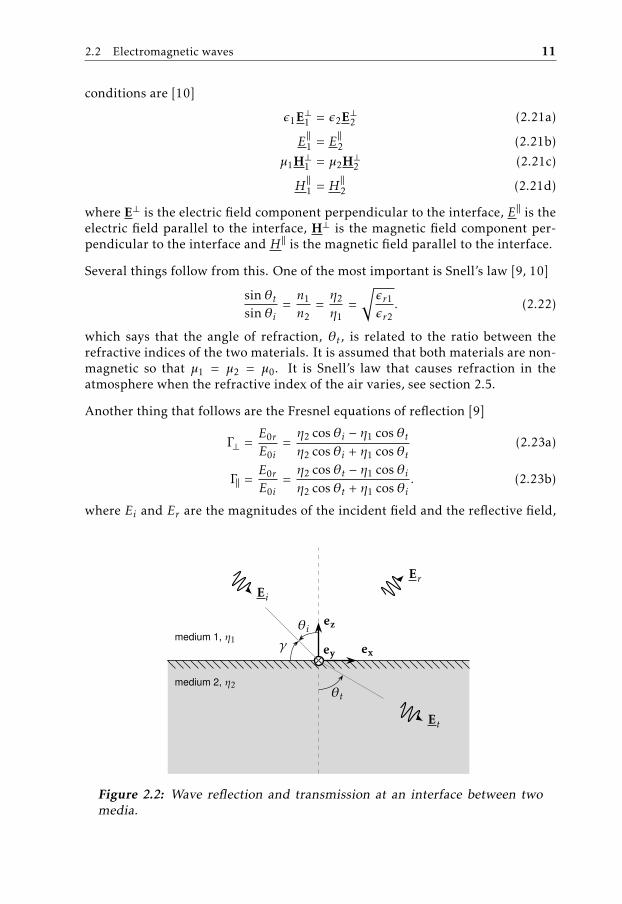
2.2.3 Boundary conditionsAt the interface between two different materials, Maxwell’s equations give someboundary conditions that have to be fulfilled by the field on both sides of theboundary. The situation at the interface can be seen in Figure 2.2. The boundary

2.2 Electromagnetic waves 11

conditions are [10]

ϵ1E⊥1 = ϵ2E

⊥2 (2.21a)

E∥1 = E∥2 (2.21b)

µ1H⊥1 = µ2H

⊥2 (2.21c)

H∥1 = H∥2 (2.21d)

where E⊥ is the electric field component perpendicular to the interface, E∥ is theelectric field parallel to the interface, H⊥ is the magnetic field component per-pendicular to the interface and H∥ is the magnetic field parallel to the interface.

Several things follow from this. One of the most important is Snell’s law [9, 10]

sin θtsin θi

=n1n2

=η2η1

=√ϵr1ϵr2

. (2.22)

which says that the angle of refraction, θt , is related to the ratio between therefractive indices of the two materials. It is assumed that both materials are non-magnetic so that µ1 = µ2 = µ0. It is Snell’s law that causes refraction in theatmosphere when the refractive index of the air varies, see section 2.5.

Another thing that follows are the Fresnel equations of reflection [9]

Γ⊥ =E0rE0i

=η2 cos θi − η1 cos θtη2 cos θi + η1 cos θt

(2.23a)

Γ∥ =E0rE0i

=η2 cos θt − η1 cos θiη2 cos θt + η1 cos θi

. (2.23b)

where Ei and Er are the magnitudes of the incident field and the reflective field,

medium 1, η1

medium 2, η2

ey ex

ez

Ei

θiγ

Et

θt

Er

Figure 2.2: Wave reflection and transmission at an interface between twomedia.

12 2 Theory

respectively as indicated in Figure 2.2. The quantity Γ relates the reflected fieldto the incident field. The difference between Γ⊥ and Γ∥ is that they correspondto the cases where the incident field is polarized perpendicular or parallel to theplane of the interface, respectively. So, in the first case the polarization vectores⊥ is perpendicular to the normal of the interface en = ez in Figure 2.2, so thates⊥ · en = 0. In the case of parallel polarization, es∥ · en ≠ 0. The Fresnel equationsof reflection are not of much use to the current study in their present form. It ispreferably to be able to express them in terms of the grazing angle, γ , which is thecomplementary angle to the incident angle θi (see Figure 2.2) and the mediumimpedance η. One then finds that [2, 11]

R+0 = Γ∥ =

Y sin γ −√Y − cos2 γ

Y sin γ +√Y − cos2 γ

(2.24a)

R−0 = Γ⊥ =sin γ −

√Y − cos2 γ

sin γ +√Y − cos2 γ

(2.24b)

where Y = η21 /η22 = n22/n

21 = ϵr1/ϵr2, and where for the second equality it is as-

sumed that µ1 = µ2 = µ0 for a non-magnetic media [9]. The reflection coefficientscan be used to calculate the field that is reflected off the interface and will be usedlater in the boundary conditions and the implementation of ground in the model.

The explicit notation for phasors, E, is dropped after this section for notationalsimplicity. All quantities related to the fields E and B are still considered to bephasors unless explicitly noted.

2.3 The parabolic equationSolving the Helmholtz equation is, in general, an easier problem than solvingMaxwell’s equations, but a quite difficult problem nevertheless. To make thiseasier, it is common to do some additional approximations and solve a simplifiedproblem instead. In the field of propagation of radio waves, the most common isto use a parabolic equation to describe the propagation.

The parabolic approximation was first described by Leontovich and Fock [12]. Itdid not become popular until an algorithm, the ssfm, to efficiently solve it waspresented by Hardin and Tappert [13] in 1973 and the computational power incomputers had advanced sufficiently.

This section presents the derivation of the parabolic equation for both a flat and aspherical Earth. The situation that we want to calculate can be seen in Figure 2.3.

2.3.1 Flat EarthIn the case of a flat Earth, the coordinate system seen in Figure 2.3 is an ordinaryCartesian one, since the coordinate ex along the surface of the Earth is a straightline. The derivation of the parabolic equation starts with the Helmholtz equationobtained above (

∇2 + k2n2)ψ = 0 (2.25)

2.3 The parabolic equation 13

ey ex

ez

paraxial direction

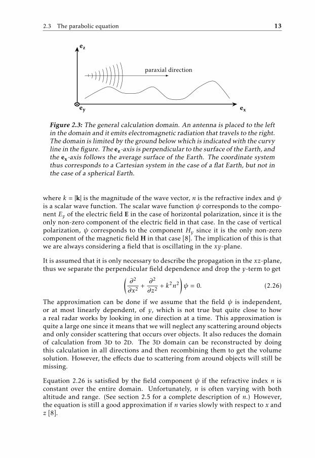
Figure 2.3: The general calculation domain. An antenna is placed to the leftin the domain and it emits electromagnetic radiation that travels to the right.The domain is limited by the ground belowwhich is indicated with the curvyline in the figure. The ez-axis is perpendicular to the surface of the Earth, andthe ex-axis follows the average surface of the Earth. The coordinate systemthus corresponds to a Cartesian system in the case of a flat Earth, but not inthe case of a spherical Earth.

where k = |k| is the magnitude of the wave vector, n is the refractive index and ψis a scalar wave function. The scalar wave function ψ corresponds to the compo-nent Ey of the electric field E in the case of horizontal polarization, since it is theonly non-zero component of the electric field in that case. In the case of verticalpolarization, ψ corresponds to the component Hy since it is the only non-zerocomponent of the magnetic fieldH in that case [8]. The implication of this is thatwe are always considering a field that is oscillating in the xy-plane.

It is assumed that it is only necessary to describe the propagation in the xz-plane,thus we separate the perpendicular field dependence and drop the y-term to get(

∂2

∂x2+∂2

∂z2+ k2n2

)ψ = 0. (2.26)

The approximation can be done if we assume that the field ψ is independent,or at most linearly dependent, of y, which is not true but quite close to howa real radar works by looking in one direction at a time. This approximation isquite a large one since it means that we will neglect any scattering around objectsand only consider scattering that occurs over objects. It also reduces the domainof calculation from 3d to 2d. The 3d domain can be reconstructed by doingthis calculation in all directions and then recombining them to get the volumesolution. However, the effects due to scattering from around objects will still bemissing.

Equation 2.26 is satisfied by the field component ψ if the refractive index n isconstant over the entire domain. Unfortunately, n is often varying with bothaltitude and range. (See section 2.5 for a complete description of n.) However,the equation is still a good approximation if n varies slowly with respect to x andz [8].

14 2 Theory

We introduce the reduced wave function

u(x, z) = ψ(x, z)e−jkx. (2.27)

This is done by assuming that the energy is mainly propagating in the x-direction,and, by doing this change of variable, rapid oscillations due to the carrier waveof the field are factored away [14]. This gives a field u that is varying slowly withrespect to x [8].

Substituting u, defined in Equation 2.27, into Equation 2.26 and performing thedifferentiations on the exponential gives[

∂2

∂z2+∂2

∂x2+ 2jk

∂∂x

+ k2(n2 − 1

)]u(x, z) = 0. (2.28)

To further simplify the expression, it is assumed that∂2u∂x2

≪

2jk

∂u∂x

(2.29)

which is known as the paraxial or the parabolic approximation. This approxi-mation is part of the method to simplify the expression. The approximation isdone on the grounds that the reduced function is a slowly varying function in x[15]. The approximation means that the solution will be limited to fields that arepropagating close to the so-called paraxial direction [14]. The paraxial directionis the main direction of the propagation of the waves, in this case, the x-direction,see Figure 2.3.

The paraxial approximation lets us remove the small second derivative with re-spect to x, and the standard parabolic equation[

∂2

∂z2+ 2jk

∂∂x

+ k2(n2 − 1

)]u(x, z) = 0. (2.30)

is obtained which is often used as the starting point of many authors, e.g. [16, 17].At this stage it is noted that this equation is a first order differential equation withrespect to x, something that will become crucial when attempting to solve it.

2.3.2 Round EarthIn the case of a spherical Earth, things are slightly more complicated since theex-axis in Figure 2.3 no longer corresponds to a straight line in reality. Therefore,it is necessary to do a transformation to obtain a rectangular domain. The deriva-tion follows the same steps, except for a coordinate transform to account for thespherical Earth.

We start by imagining the Earth as a sphere with radius ae, on which we place theradar antenna at the top. If we introduce an ordinary spherical coordinate system(r, θ, φ) with the origin at the centre of the Earth, the antenna will be placed inthe point (ae + ha, 0, φ). The origin of the domain in Figure 2.3 corresponds tothe point (ae, 0, φ) in this coordinate system. It is possible to set up Maxwell’sequations for this situation, and from there derive the Helmholtz equation if weassume azimuthal independence. However, we want to represent the Helmholtz

2.3 The parabolic equation 15

equation in the coordinate system in Figure 2.3 where the coordinates have aneasy interpretation. This can be done using a conformal transformation if wewrite the planes xz and rθ as complex variables using

Ξ = x + jz, ζ = (ae + h)(sin (θ) + j cos (θ)). (2.31)

The Möbius transformation corresponding to the relation between the two coor-dinate systems is then [18]

Ξ = 2aeae + jζζ + jae

, (2.32)

where ae is the radius of the Earth.

It is then possible to approximate the Möbius transformation using these rela-tions between the coordinate systems [8]⎧⎪⎪⎪⎪⎨⎪⎪⎪⎪⎩

x = aeθ

z = ae ln(1 +

hae

)≈ h

(2.33)

where ae is the radius of the Earth and h the height above the surface of theEarth. The coordinate θ comes from the spherical coordinate system. The lastapproximation is valid for the region where z, x ≪ ae [18].

This gives that the Helmholtz equation, Equation 2.26, can be transformed andwritten in the new coordinate system, seen in Figure 2.3, as [8, 18](

∂2

∂x2+∂2

∂z2+

dζdΞ

2k2n(x, z)2

)ψ = 0 (2.34)

where the scalar field ψ relates to the electric and magnetic fields as [8, 18]

ψh =

√kae sin

(xae

)exp

(z2ae

)Eφ, Horizontal polarization (2.35a)

ψv =

√ϵ0ϵ

√kae sin

(xae

)exp

(z2ae

)Hφ, Vertical polarization. (2.35b)

We introduce a reduced wave function u here as well to obtain[∂2

∂z2+∂2

∂x2+ 2jk

∂∂x

+ k2(dζdΞ

2n2 − 1

)]u(x, z) = 0, (2.36)

which is very similar to Equation 2.28 in the previous subsection. As before, thenext step is to do the parabolic approximation, but here we also do the approxi-mation that [18],

k2(dζdΞ

2n2 − 1

)≈ k2

(n2 − 1 +

2zae

)=: k2(m2 − 1), (2.37)

where we have introduced a modified index of refraction m2 = n2 + (2z)/ae that

16 2 Theory

includes a term that accounts for the curvature of the Earth. The exact require-ments for this approximation can be found in [18]. Using the notation m givesthe parabolic equation for the case of the spherical Earth on the same form as forthe flat Earth [

∂2

∂z2+ 2jk

∂∂x

+ k2(m2 − 1

)]u(x, z) = 0, (2.38)

but with a different interpretation of u due to the new interpretation of the scalarwave function ψ in Equation 2.35. This is the version of the parabolic equationthat will be used for the rest of the thesis.

2.4 The split-step Fourier methodThe split-step Fourier method was presented as an algorithm intended to solvethe parabolic wave equation by Hardin and Tappert [13] in 1973. The method is amarching method which means that it successively calculates the next step fromthe previous one. I.e., given the field at an initial point, u(x = x0, z), the ssfmenables the calculation of the entire domain by calculating first u(x = x1, z) andthen u(x = x2, z) etc., up to some maximum x-value, given that the steps xi+1 − xiare small enough.

What makes this method special is that half of the marching takes place in thespatial domain, while the other part takes place in the Fourier domain. So thesolution is advanced in half steps. This will become clearer at the end of thissection.

The following section is dedicated to the derivation of a propagator, or an evolu-tion operator, that is used to march the solution forward. This section containstwo different methods to get to such a propagator under different approxima-tions. The different methods used to obtain them causes the propagators to beslightly different and to have different precision.

2.4.1 Method 1Themethod to obtain a propagator follows the outline presented by Agrawal [19].We start with the parabolic equation Equation 2.38. The parabolic equation canbe rewritten in a more convenient form

∂u∂x

=[j

2k∂2

∂z2+jk

2

(m(x, z)2 − 1

)]u(x, z), (2.39)

which highlights the fact that it is a partial differential equation of the first orderwith respect to x.

This version of the parabolic equation can be restated in a more compact form as

∂u∂x

=[L + N

]u(x, z), (2.40)

with the help of the two operators L and N , defined as

L :=j

2k∂2

∂z2N :=

jk

2

(m(x, z)2 − 1

). (2.41)

2.4 The split-step Fourier method 17

Equation 2.40 has a solution that can be expressed using the operators N and L.The solution is formally

u(x + ∆x, z) = e(L+N

)∆xu(x, z), (2.42)

for a ∆x that is small enough and under the assumption that the operators areboth independent of x. This assumption is not entirely true since m in general isa function of both x and z. But for small variations of m, this is approximatelytrue. We assume that m is almost constant, or at least that it varies slowly withrespect to x.

The factorization of the exponential operator can be approximated using a Suzuki-Trotter decomposition [20] which can be written

eδAeδB = eδ(A+B)+12 δ

2[A,B]+O(δ3). (2.43)

We perform the decomposition with the same designations as in [8]

A =1k2

∂2

∂z2, B = m(x, z)2 − 1, δ =

jk∆x

2, (2.44)

so A and B are L and N with the term jk/2 factored out, jkA/2 = L, jkB/2 = L.Doing this gives the approximate solution u(x + ∆x, z) as

u(x + ∆x, z) ≈ eδAeδBu(x, z) = e∆xLe∆xNu(x, z), (2.45)

where we have disregarded the quadratic error term exp (0.5δ2[A, B]). The errorintroduced when doing this obviously scales with δ2, and thereby with (∆x)2, butthe term δ is not small in general. It is common to have ∆x on the order of 100mand k ∝ 10m−1 for normal radar frequencies. However, it is assumed that A andB almost commute, so that the error term becomes small due to the small com-mutator. The next error term includes nested commutators, [15], and is assumedto be smaller still. It is also possible to calculate the decomposition using a sym-metric Suzuki-Trotter decomposition eδ(A+B) = e(δA)/2eδBe(δA)/2 + O(δ3) [20]. Thisis more exact, but is for simplicity not used here.

The next step is to calculate the solutions for the operators N and L separately.We assume that we have two different regions. One region is in which the wave ispropagating through vacuum so that the operator N becomes 0. The other regionis where the refractive effects are taken into account, and there the diffractionoperator L is taken to be zero. So, each marching step is made up of two steps:one with free space propagation and one with only refraction. This can be seenas a system where the wave propagates through a series of thin lenses placed invacuum [21].

Inside the lens, L is taken to be zero, then the parabolic equation, Equation 2.40,can be written as

∂u∂x

= N u(x, z) =jk

2

(m(x, z)2 − 1

)u(x, z). (2.46)

18 2 Theory

This version of the parabolic equation has the solution

u(x + ∆x, z) = exp

⎛⎜⎜⎜⎜⎜⎜⎜⎝x+∆x∫x

N dx′

⎞⎟⎟⎟⎟⎟⎟⎟⎠u(x, z)= exp

⎛⎜⎜⎜⎜⎜⎜⎜⎝ jk2x+∆x∫x

m2(x′ , z) − 1 dx′

⎞⎟⎟⎟⎟⎟⎟⎟⎠u(x, z)≈ exp

(jk∆x

2

[m2

(x +

∆x2, z

)− 1

])u(x, z),

(2.47)

where the integral is due to the fact that N is dependent of x. The integral shouldtherefore actually be present in both Equation 2.42 and Equation 2.45 as well toaccount for this. In the third step, the integral has been approximated with themidpoint rule. This approximation should not introduce any large errors eventhough it is a crude approximation in most cases. It has already been said thatm is almost independent of x since it is almost constant. If it is constant, or ifm2 would vary linearly, then the midpoint rule is exact, and it can therefore beexpected to be reasonably accurate for something that is almost constant.

For the case of the free space propagation, where N is zero and we only considerthe operator L, the parabolic equation, Equation 2.40, reduces to

∂u∂x

= Lu(x, z) =j

2k∂2

∂z2u(x, z). (2.48)

This equation is most easily solved in the Fourier domain. Taking the Fouriertransform with respect to z yields

∂u∂x

=−jp2z2k

u(x, pz), (2.49)

where u is the wave function in the Fourier domain corresponding to the wavefunction u in the spatial domain. The equation has the exact solution

u(x + ∆x, pz) = exp(−j∆xp2z2k

)u(x, pz). (2.50)

Now, both these solutions, Equation 2.47 and Equation 2.50, that are valid ineach part of space are combined together by the help of Equation 2.45 to geta propagator that takes the solution from one step x to the next x + ∆x. Thiscombined solution is expressed as

u(x + ∆x, z) = exp(jk∆x

2

[m2

(x +

∆x2, z

)− 1

])F −1

exp

(−j∆xp2z2k

)F u(x, z)

.

(2.51)

This propagator is what is referred to as the narrow-angle propagator by Levy

2.4 The split-step Fourier method 19

[8], even though she uses a different derivation.

All the transformations back and forth to the Fourier domain is due to the factthat we only have one propagator, Equation 2.50, in the Fourier domain. Theidea is that it is faster to move back and forth than trying to solve the entireparabolic equation in the spatial domain. The fastest way to move back and forthbetween the Fourier domain and the spatial domain is by using the Fast FourierTransform, fft. The fft is an algorithm to reduce the number of operations inthe discrete version of the Fourier transform, thereby making it faster to computefor larger vector sizes [22].

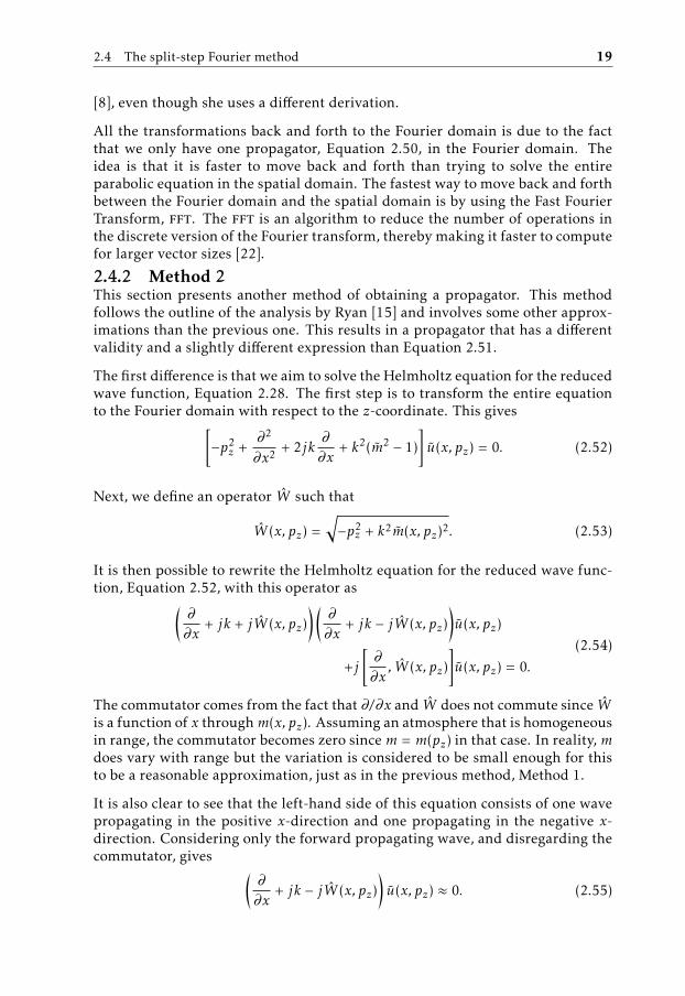
2.4.2 Method 2This section presents another method of obtaining a propagator. This methodfollows the outline of the analysis by Ryan [15] and involves some other approx-imations than the previous one. This results in a propagator that has a differentvalidity and a slightly different expression than Equation 2.51.

The first difference is that we aim to solve the Helmholtz equation for the reducedwave function, Equation 2.28. The first step is to transform the entire equationto the Fourier domain with respect to the z-coordinate. This gives[

−p2z +∂2

∂x2+ 2jk

∂∂x

+ k2(m2 − 1)]u(x, pz) = 0. (2.52)

Next, we define an operator W such that

W (x, pz) =√−p2z + k2m(x, pz)2. (2.53)

It is then possible to rewrite the Helmholtz equation for the reduced wave func-tion, Equation 2.52, with this operator as(

∂∂x

+ jk + jW (x, pz)) (

∂∂x

+ jk − jW (x, pz))u(x, pz)

+j[∂∂x, W (x, pz)

]u(x, pz) = 0.

(2.54)

The commutator comes from the fact that ∂/∂x and W does not commute since Wis a function of x throughm(x, pz). Assuming an atmosphere that is homogeneousin range, the commutator becomes zero since m = m(pz) in that case. In reality, mdoes vary with range but the variation is considered to be small enough for thisto be a reasonable approximation, just as in the previous method, Method 1.

It is also clear to see that the left-hand side of this equation consists of one wavepropagating in the positive x-direction and one propagating in the negative x-direction. Considering only the forward propagating wave, and disregarding thecommutator, gives (

∂∂x

+ jk − jW (x, pz))u(x, pz) ≈ 0. (2.55)

20 2 Theory

We do the same rearrangement of the equation to highlight it being a first orderpartial differential equation with respect to x as we did in the previous section.

∂u(x, pz)∂x

=(−jk + jW (x, pz)

)u(x, pz) = jQ(x, pz)u(x, pz), (2.56)

where we have defined an operator Q

Q(x, pz) := W (x, pz) − k =√−p2z + k2m(x, pz)2 − k. (2.57)

To get a solution that can be marched forward, we want to define an evolutionoperator U (x, x0, pz) such that it is possible to calculate the next step given theprevious step as

u(x, pz) = U (x, x0, pz)u(x0, pz), (2.58)

with x0 being some value of x smaller than x, x0 ≤ x. Substitution of this expres-sion into Equation 2.56 gives that the evolution operator U (x, x0, pz) must fulfilthe relation

∂U (x, x0, pz)∂x

= jQ(x, pz)U (x, x0, pz). (2.59)

This partial differential equation for the evolution operator has the general solu-tion

U (x, x0, pz) = eΩ(x,x0,pz ), Ω(x, x0, pz) =

∞∑k=1

Ωk(x, x0, pz), (2.60)

where Ω(x, x0, pz) is a Magnus expansion. The Magnus expansion is an infiniteseries, and the first three terms in the sum are [23]

Ω1 = j

x∫x0

Q(x1, pz) dx1 (2.61a)

Ω2 = −12

x∫x0

dx1

x1∫x0

dx2[Q(x1, pz), Q(x2, pz)

](2.61b)

Ω3 = −j

6

x∫x0

dx1

x1∫x0

dx2

x2∫x0

dx3([Q1,

[Q2, Q3

]]+

[Q3,

[Q2, Q1

]]), (2.61c)

where in the last term, the notation Q1 = Q(x1, pz), Q2 = Q(x2, pz) and Q3 =Q(x3, pz) has been used for brevity. The infinite series is too cumbersome to han-dle, so it is approximated by its first term. This is a good approximation in mostcases since it can be noted that this is no approximation at all if the operator Qcommutes with itself for different values of x. This should hold true for Q since Qcan be evaluated to be a scalar at each point x in the Fourier domain, and scalars

2.4 The split-step Fourier method 21

always commute. Applying this assumption gives a short formulation of Ω as

Ω(x, x0, pz) = Ω1(x, x0, pz) = j

x∫x0

Q(x1, pz) dx1. (2.62)

Having expressed Ω in a closed form enables the writing of the solution of theevolution operator U . The necessary form U must have to fulfil the requirementin Equation 2.59 is

U (x, x0, pz) = exp

⎛⎜⎜⎜⎜⎜⎜⎜⎜⎝jx∫

x0

Q(x1, pz) dx1

⎞⎟⎟⎟⎟⎟⎟⎟⎟⎠. (2.63)

To simplify the evaluation of the integral, we split Q in two parts: Q(x, pz) ≈A(pz) + B(x, pz). This means that the radical in Q has to be approximated some-how. We choose another method than the one presented by Ryan [15] to do this.The operator Q can be written as

Q = k

⎛⎜⎜⎜⎜⎜⎝√−p2zk2

+ m2(x, pz) − 1

⎞⎟⎟⎟⎟⎟⎠ = k (√1 + Z + ξ − 1)

(2.64)

with

Z = −p2zk2, ξ = m2(x, pz) − 1. (2.65)

Doing a first order Taylor series around ξ = 0 gives√1 + Z + ξ =

√1 + Z +

ξ

2√1 + Z

+ O(ξ2), (2.66)

and then doing another Taylor series expansion around Z = 0 in the second termgives √

1 + Z + ξ =√1 + Z +

ξ2+ O(Zξ) (2.67)

This is the approximation used in [24]. Then we can put A(pz) =√1 + Z =√

k2 − p2z − k, and B(x, pz) = (k/2)(m2(x, pz) − 1). Compare these two operators

A and B with the operators L and N that were defined in the previous section.

Using these operators, the integral in the exponent in Equation 2.63 can be sepa-rated as

x∫x0

Q(x1, pz) dx1 ≈ (x − x0)A(pz) +x∫

x0

B(x1, pz) dx1. (2.68)

22 2 Theory

Thus, the evolution operator becomes (with ∆x := x − x0)

U (x, x0, pz) = exp

⎛⎜⎜⎜⎜⎜⎜⎜⎜⎝j∆xA(pz) + jx∫

x0

B(x1, pz) dx1

⎞⎟⎟⎟⎟⎟⎟⎟⎟⎠. (2.69)

We want to split the sum in the exponent to get the right form of the propaga-tor to fit with the split-step algorithm. This is done by the same Suzuki-Trotterdecomposition [20] as was done in the first method

exp(j∆xA(pz)

)exp

⎛⎜⎜⎜⎜⎜⎜⎜⎜⎝jx∫

x0

B(x1, pz) dx1

⎞⎟⎟⎟⎟⎟⎟⎟⎟⎠ ≈≈ exp

⎛⎜⎜⎜⎜⎜⎜⎜⎜⎝j∆xA(pz) + jx∫

x0

B(x1, pz) dx1

⎞⎟⎟⎟⎟⎟⎟⎟⎟⎠.(2.70)

The propagator B is easier to calculate in the spatial domain, since n has a mean-ing there. So, we return B to the spatial domain via an inverse Fourier trans-form. It is assumed that such a transform exists since n represents a physicalproperty and can therefore be considered to be sufficiently well-behaved. There,B(x1, z) = (k/2)(m(x1, z)2 − 1). This causes half of the propagator to be calculatedin the spatial domain, and half in the Fourier domain.

So, inserting the expressions of A and B into Equation 2.70, and switching theorder of the exponents (that now only are scalars), the full propagator becomes

U (x, x0, z) = exp

⎛⎜⎜⎜⎜⎜⎜⎜⎜⎝ jk2x∫

x0

(m2(x1, z) − 1

)dx1

⎞⎟⎟⎟⎟⎟⎟⎟⎟⎠F −1

exp

(j∆x

(√k2 − p2z − k

)).

(2.71)

It is possible to use the midpoint rule here as well to approximate the integral.This puts the two propagators on the same form, making them easier to compare.Doing this yields a propagator that gives the next step as:

u(x + ∆z, z) = exp(jk∆x

2

(m2(x0 +

∆x2, z) − 1

))F −1

exp

(j∆x

(√k2 − p2z − k

))F u(z, x)

.

(2.72)

This propagator is very similar to what is referred to as the wide-angle propagatorby Levy [8]. The difference is in the environment term where she obtains m − 1instead of the current (m2 − 1)/2. This comes from different approximations ofthe radical in Q, Equation 2.64.

2.4 The split-step Fourier method 23

Both propagators that are obtained by the twomethods are presented in Table 2.1for easier comparison. The propagator derived in this section, Equation 2.72,has the same environmental term as the one defined in the previous method,Equation 2.51, what differs between them is the free space term. It can also beseen that the free space term in Equation 2.51 is a Taylor expansion of the rationalto the first order of the free space term in Equation 2.72. This is reassuring, sinceit means that both propagators should describe the same phenomena.

2.4.3 Sampling distanceOne of the main steps in these methods is the Fourier transform. This meansthat the signal will be moved to the Fourier domain and then back. The signalwill thus have to be sampled in accordance with the sampling theorem to avoidaliasing and distortion of the signal [25]. This is very important since the recon-struction of the signal occurs several times in each step, meaning that a smallreconstruction error each time will accumulate to become a very large recon-struction error in the end.

A function x(t) that has a Fourier transform that exists, and equals zero for |ω| >2πB is said to be band-limited, where B is its bandwidth. Such a function canbe uniquely reconstructed by sampling the signal with a sampling distance of1/2B, the sampling theorem [26]. The reduced wave function, u(z), is assumedto be band-limited with the bandwidth pmax, since the Fourier transform of u isassumed to be zero above this value, u(pz) = 0 for |pz | > pmax [18]. The samplingtheorem then says that this band-limited function can be uniquely reconstructedfrom its transform for all points z if the sample points are spaced π/pmax z-unitsapart, or closer. The spacing in z is equal to ∆z = zmax/Nz , where zmax is thelargest z of interest, the top of the domain, and Nz is the number of samplesin the z-direction. But the sample spacing is also, from the sampling theorem,∆z ≤ π/pmax. So, we get that the minimum number of sample points in the z-direction is Nz ≥ (zmaxpmax)/π.

Table 2.1: A comparison between the narrow angle propagator obtained us-ing method 1 and the wide angle propagator using method 2.

Environmentalterm:

Narrow angle: exp(jk∆x

2

[m2

(x +

∆x2, z

)− 1

])Wide angle: exp

(jk∆x

2

[m2

(x +

∆x2, z

)− 1

])

Free spaceterm:

Narrow angle: exp(−j∆xp2z2k

)

Wide angle: exp

⎛⎜⎜⎜⎜⎜⎝j∆xk⎛⎜⎜⎜⎜⎜⎝√1 −

p2zk2− 1

⎞⎟⎟⎟⎟⎟⎠⎞⎟⎟⎟⎟⎟⎠

24 2 Theory

The variable pz is interesting. Within the interval −pmax < pz < pmax it can beinterpreted as pz = k sinα, where k is the magnitude of the wave vector and αis the angle from the x-axis. Then the maximum value pmax can be calculatedas pmax = k sinαmax where αmax is the maximum angle of interest [18]. In thiscontext, it is also possible to see αmax as the angle corresponding to the wave withthe highest elevation that can be correctly reconstructed.

Using this in the requirement on Nz gives that

Nz ≥zmaxpmax

π=zmaxk sinαmax

π=

2zmax sinαmaxλ

, (2.73)

if we use that k = (2π)/λ, with λ being the wavelength of the signal. This is acondition that is easier to fulfil than the earlier expression since | sinα| always issmaller than one regardless of the angle α. This limitation can also be expressedas a requirement on ∆z

∆z ≤ λ2 sinαmax

(2.74)

which is almost always larger than λ in a realistic case. In the parabolic approx-imation, it was assumed that the waves were propagating forward with a smallangle relative to the surface. This means that the angle αmax does not have to bevery large to include all the waves, and thus the spacing ∆z can be quite large.An example of 20GHz and an angle of 5° gives that ∆z should be at least equalto 8.6 cm, which is larger than the wavelength, 1.5 cm.

2.4.4 Initial fieldThe initial field is of great importance since the split-step Fouriermethodmarchesa solution forward. So, the initial field will be the basis for the entire solution.

The initial field used in this study is the one described by Levy [8]. It represents aGaussian beam pattern propagated to the far-field, so that the antenna is outsideof the domain, and is written as

uf s(0, z) =kβ

2√2π ln 2

exp (−jkθ0z) exp(−

β2

8 ln 2k2(z − ha)2

)(2.75)

where θ0 is the elevation angle of the antenna compared with the surface at thesite of the antenna, β is the half-power beam width of the antenna, ha is thealtitude of the antenna over the ground and k is the wave vector of the signal.

We want the initial field to satisfy the boundary conditions. This is done by usingimage theory and assuming a perfectly conducting ground. Then the initial fieldat x = 0 can be written as

u(x = 0, z) =

⎧⎪⎪⎨⎪⎪⎩uf s(0, z) − uf s(0,−z) Horizontal polarizationuf s(0, z) + uf s(0,−z) Vertical polarization

(2.76)

This field is then what is marched out over the entire domain.

2.5 The atmosphere 25

2.5 The atmosphereSince the propagation of the em-waves takes place in the atmosphere, the electro-magnetic properties of the atmosphere become important. The most importantelectromagnetic properties of the atmosphere can be summarized in the index ofrefraction, n. The index of refraction of a material is a ratio that describes howfast light propagates in that material compared to vacuum. This ratio is given as[27]

n =c0v, (2.77)

where v is the speed of light in the current medium and c0 is the speed of lightin vacuum. For air, the index of refraction is almost 1, it seldom exceeds 1 withmore than a fraction on the order of 1 × 10−4. It is usually around 1.0003 for air[28]. This makes n quite a cumbersome unit, so the refractivity is introduced as[29]

N := (n − 1) × 106, (2.78)

for a real index of refraction. The refractivity is measured in N-units, [30].

The refractivity of the atmosphere is a function of the temperature, pressure andhumidity as described by [28, 29]

N = 77.6PTe

+ 3.73 × 105 ewT 2e, (2.79)

where P is the atmospheric pressure in millibars, Te is the temperature in Kelvinand ew is the partial pressure of water vapour in millibars that is calculated as[29]

ew = esHR = 6.1 exp(25.22

Te − 273Te

− 5.31 ln( Te273

)), (2.80)

where es is the saturated water pressure in millibars and HR is the relative hu-midity in percent.

Most of the time, it is possible to use the approximation of a standard atmosphererather than having to know all the parameters in the equation above. For a stan-dard atmosphere, the refractivity is a function of the altitude. It decreases withaltitude according to [30]

N (z) = 315e−0.136z , (2.81)

where z is the altitude in km above the sea surface. This can be seen in the leftpart of Figure 2.4. This causes the em-waves to bend downwards in a standard at-mosphere, in accordance with Snell’s law, which is explained in subsection 2.2.3.So, a ray that is launched parallel to the surface of the Earth will bend downslightly. It will bend down with a curvature corresponding to a circle with a ra-dius approximately 4/3 of that of the Earth. This is why 4/3 times the radius ofthe Earth, together with straight rays can be used for calculations, since that in-corporates the effects of the atmosphere [3]. Using an Earth radius 4/3 times theactual one will cause rays to go straight which simplifies matters [2]. This is a

26 2 Theory

very common approximation, but it is seldom explained why it is done.

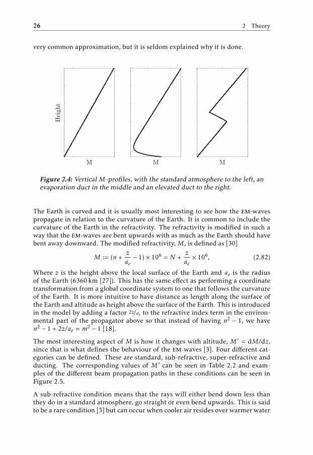
Figure 2.4: VerticalM-profiles, with the standard atmosphere to the left, anevaporation duct in the middle and an elevated duct to the right.

The Earth is curved and it is usually most interesting to see how the em-wavespropagate in relation to the curvature of the Earth. It is common to include thecurvature of the Earth in the refractivity. The refractivity is modified in such away that the em-waves are bent upwards with as much as the Earth should havebent away downward. The modified refractivity,M, is defined as [30]

M := (n +zae− 1) × 106 = N +

zae× 106, (2.82)

Where z is the height above the local surface of the Earth and ae is the radiusof the Earth (6360 km [27]). This has the same effect as performing a coordinatetransformation from a global coordinate system to one that follows the curvatureof the Earth. It is more intuitive to have distance as length along the surface ofthe Earth and altitude as height above the surface of the Earth. This is introducedin the model by adding a factor 2z/ae to the refractive index term in the environ-mental part of the propagator above so that instead of having n2 − 1, we haven2 − 1 + 2z/ae = m2 − 1 [18].

The most interesting aspect of M is how it changes with altitude, M ′ = dM/dz,since that is what defines the behaviour of the em-waves [3]. Four different cat-egories can be defined. These are standard, sub-refractive, super-refractive andducting. The corresponding values of M ′ can be seen in Table 2.2 and exam-ples of the different beam propagation paths in these conditions can be seen inFigure 2.5.

A sub-refractive condition means that the rays will either bend down less thanthey do in a standard atmosphere, go straight or even bend upwards. This is saidto be a rare condition [3] but can occur when cooler air resides over warmer water

2.5 The atmosphere 27

Earth

ducting

super-refractive

standard

sub-refractive

Figure 2.5: The different categories of wave propagation in the atmosphere.

Table 2.2: The different refraction conditions expressed inM ′ [30].

Refraction type M ′ = dM/dz

Sub-refractive > 118Standard 118Super-refractive < 118Ducting < 0

[31]. This will decrease the range of the signal, since it disappears up into space.

A super-refractive condition is when the rays bend down more sharply than ina standard atmosphere. This will cause the em-waves to follow the surface ofthe Earth longer, thereby increasing the range of the system. Super-refractiveconditions may occur when warmer air resides over cooler water [31].

Other atmospheric phenomena such as precipitation also affect the propagation.It causes both absorption and scattering. Some of the scattered radiation hitsthe receiving antenna and are seen as echoes. This is desirable in the case ofa weather radar, but in any other case, it is considered as a problem. It is ingeneral very hard to model the effect of precipitation exactly as the effects takeplace at a very small level, the size of snowflakes or raindrops, which makes itimpossible to do a calculation for a large domain due to the higher resolutionnecessary. It is therefore common to model precipitation as a dampening of thesignal with some decibel per kilometre [2]. The attenuation is strongly frequencydependent with higher frequencies experiencing larger attenuation. For a wave-length of 0.3 cm, the attenuation ranges from 0.305 to 46dBkm−1 for rain ratesof 0.25 to 150mmh−1. For a wavelength of 10 cm it is much less, from 1 × 10−5to 0.0481dBkm−1 for the same rain rates [2]. This is a very strong dampeningfor, especially for 150mmh−1 which however might be an unreasonable rain ratefor Swedish conditions. A more normal rain rate, 2.5mmh−1, considered to be a

28 2 Theory

moderate rain by the Swedish Meteorological and Hydrological Institute, smhi,[32] gives an attenuation of 0.0388dBkm−1 for a 10GHz signal [2].

2.5.1 DuctingDucting is an extreme case of a super-refractive condition. A duct is any con-dition with a negative M-gradient. Two different cases of ducts can be seen inFigure 2.4, an evaporation duct in the middle and an elevated duct to the right inthe figure. A duct can be seen almost as a waveguide that is open on the top [3]this makes it possible for the waves to travel very long distances.

The propagation in a duct is guided, which makes it possible for the waves to thetravel very far. The rays will bounce off the top and bottom of the duct, like in awaveguide, or in the case of a ground-based duct, the ground, and the top of theduct. However, this is only true for angles that are very close to the direction ofthe duct. When an em-wave hits the duct at a larger angle, its propagation willbe hindered by the duct [2–4].

Ducts can be separated into two categories depending on the height at whichthey appear: ground-based ducts and elevated ducts. A ground-based duct canbe due to a temperature inversion, such as the case when warm dry air flowsout over cool water. It is also possible to get a temperature inversion when theground that has been significantly heated by the sun during the day is cooledoff while the air keeps the same temperature [4]. Ground-based ducts can alsoappear as evaporation ducts. The air just above the sea surface is saturated andthus contains much water vapour. At higher altitudes it does not, and so the ductis formed. Evaporation ducts are present over all water bodies almost all the time[3].

Elevated ducts can be formed by what is called subsidence. This is when coolerair moves downwards. This causes the air to undergo adiabatic heating due tothe increase of pressure which causes the moisture content to decrease. This air,that now is warmer, places itself on top of the cooler, more moist air below. Thuscausing a temperature inversion [3, 4].

2.5.2 Effect on radar applicationThis subsection gives two examples of how atmospheric conditions can affect aradar system. One of them can be seen to the left in Figure 2.6. The figure showsa radar antenna placed in an elevated duct. The elevated duct causes the beamfrom the antenna to follow the duct as it traces the terrain profile. This causes thecoverage of the radar system to be far from homogeneous, with blind spots. Theaircraft seen to the right in the figure is placed in such a blind spot which meansthat it is virtually invisible for the radar system, [29]. Knowledge of the refractiveconditions might mean that a mobile antenna can be placed somewhere else, sothat the aircraft becomes visible.

The other case, seen to the right in Figure 2.6, is when the radar system believesthe target to be somewhere it is not. It can be seen in the figure that the beamfrom the antenna is refracted upwards to the target. When the rays return to theantenna, the angle of arrival corresponds to a lower altitude of the target than

2.6 Boundary conditions 29

Actual target

Apparent target

Figure 2.6: Effects of anomalous radar propagation. Left: An elevated ductcauses blind spots in the radar coverage. Adapted from [29]. Right: Sub-refractive conditions causes the radar system to misinterpret the altitude ofthe target.

what it actually is. This causes the system to misjudge the position of the target[3]. Knowledge of the refractive conditions could help minimize this effect, bytaking the refraction into consideration when interpreting the echo.

Knowledge about the refractive conditions can generally help minimize the effectof anomalous propagation and thereby making the system more reliable. It istherefore important to be able to model these effects properly.

2.6 Boundary conditionsThe domain in this type of calculation is a bit special since it is a semi-infinitedomain. The domain is supposedly infinite upwards and in the direction of prop-agation, but it is limited by the Earth. The method to handle the contact with theEarth is very different from how the other limits are handled.

2.6.1 GroundThe boundary conditions with the ground are defined by the boundary condi-tions imposed by Maxwell’s equations on the interface between two materials.Those are briefly described in section 2.2. The interface in question here is theinterface between the air and the ground, which can be made up of both soilor water, so the term ground applies to both land and sea. In this work, theem-field inside the ground is rapidly attenuated and of no interest, so only thereflections are considered. The field simulated with the parabolic equation andthe ssfm, section 2.3, corresponds to either the E or the H field, so there are onlytwo boundary conditions that have to be satisfied for each case. It is possibleto replace these two boundary conditions with a single one, a Robin boundarycondition, if the skin depth of the second material, the ground, is small [15, 33].Small in this case should be understood as small compared to the radius of theEarth [29].

The definition of skin depth is given in section 2.2 above. The frequency range of

30 2 Theory

interest in this study is 1–20GHz, at these frequencies the skin depth of seawater,at 20 C and with a salinity of 35 g kg−1 is approximately 0.2–0.001m [34]. Forsoil, it depends on the water content of it, but for dry soil with a volumetric watercontent of 0.07 the skin depth is on the order of 10 cm, [34]. All these values aremuch smaller than the radius of the Earth, 6360 km [27]. So the use of a Robinboundary condition is acceptable. A Robin boundary condition looks like

∂u∂z

z=0

+ αu(z = 0) = 0, (2.83)

for some value of α and u being the same reduced wave function as in the othersections. This boundary condition is also known as a Leontovich boundary con-dition [33].

The parameter α is calculated using the Fresnel reflection coefficients, R0 calcu-lated in subsection 2.2.3, through, [18]

α = jk cos (θi)(1 − R0

1 + R0

), (2.84)

which can be approximated as [5, 15, 18, 29]

α = jk√ϵr − 1ϵr

Vertical polarization (2.85a)

α = jk√ϵr − 1 Horizontal polarization, (2.85b)

since it is possible to assume that the incident angle is close to 90° or that the graz-ing angle is close to 0°, because the altitude of the radar antenna is small com-pared to the propagation distance. The complex relative permittivity, ϵr = ϵc/ϵ0is calculated using the International Telecommunication Union-standard, itu[34]. In this study, fresh water is approximated as pure water in the standardand is supposed to have a temperature of 20 C. Sea water is also assumed ashaving a temperature of 20 C and a salinity of 35 g kg−1. Soil in this study is un-derstood as a silty loam soil consisting of 30.36% sand, 13.48% clay and 55.86%silt as described in Figure 7 in the standard [34]. The soil is supposed to have atemperature of 23 C.

The Leontovich boundary condition can be included in the split-step Fouriermethod by replacing the standard Fourier transform with the discrete mixedFourier transform, dmft, introduced by Dockery and Kuttler [35]. So, the ideais that the boundary condition is introduced in the unavoidable going back andforth to the Fourier domain. The transform is a discretization of Equation A.5and is given by [35]

u(i∆z) =N∑′

m=0

u(m∆z)

⎡⎢⎢⎢⎢⎢⎣α sin(πimN

)−sin

(πiN

)∆z

cos(πimN

)⎤⎥⎥⎥⎥⎥⎦ , (2.86)

where ∆z is the distance between the sample points in the z-direction, N is thenumber of sample points in z and u is the reduced wave function. The prime onthe sum means that the first and the last terms are scaled with a factor 0.5. The

2.6 Boundary conditions 31

algorithm used to calculate the transform is well described in [35].

Thedmft is able to include any lossy boundary, but a simpler case is if the groundcan be considered to be a pec. Then, the requirement is that the field is zero atthe boundary in the case of horizontal polarization and that the derivative is zeroat the boundary in the case of vertical polarization. Thus, corresponding to aDirichlet or Neumann boundary condition, respectively. This can be easily satis-fied by the use of a sine Fourier transform, Equation A.1, in the case of horizontalpolarization or a cosine Fourier transform, Equation A.3 in the case of verticalpolarization [6, 36].

2.6.2 TerrainThere are several ways to account for terrain. Two different ones are describedhere: the terrain masking approach and the piecewise linear shift map.

The terrain masking approach is the easier of the two. In this method, the fieldis simply put to zero where terrain is present. It gives realistic results despite itsrather crude approach [37].

The piecewise linear shift map is a more sophisticated method. The ssfm is lim-ited in that it has to be applied to a rectangular domain. In the case of a com-plicated terrain, the domain is not rectangular, and it is therefore necessary toperform a coordinate transformation to make the domain rectangular. This coor-dinate transform is taken from Donohue and Kuttler [37]. The new coordinatesthat are introduced are

χ(x) = x

ζ(x) = z − T (x)(2.87)

where T (x) is the elevation of the terrain.

In this new coordinate system, the Helmholtz equation becomes(∂∂χ− T ′ ∂

∂ζ

)2ψ(χ, ζ) +

∂2ψ(χ, ζ)∂ζ2

+ k2m2ψ(χ, ζ) = 0. (2.88)

In order to make the Fourier transform possible, ψ is replaced by uejθ . Whereθ is a phase function. Only considering the forward propagation the parabolicequation becomes⎡⎢⎢⎢⎢⎢⎢⎣ ∂∂χ + j

∂θ∂χ− T ′

(∂∂ζ

+ j∂θ∂ζ

)− j

√(∂∂ζ

+ j∂θ∂ζ

)2+ k2m2

⎤⎥⎥⎥⎥⎥⎥⎦ u(χ, ζ) = 0. (2.89)

The method to be applied from here on is what is known as the piecewise lin-ear shift map. The theory is presented in [37]. The first step is to put the phasefunction θ to θ = k0zT

′ + f (χ) for some constant k0 = k/√1 + T ′2 and a func-

tion f (χ) such that f ′(χ) = k0(T ′2 − 1). The radical in the expression abovecan be written as K

√1 + a + b + c. An approximation to this is K

√1 + a + b + c ≈

32 2 Theory

K√1 + a + K

√1 + b + 0.5Kc − K , where

K2 = k2 − k20T′2, a =

1K2

∂2

∂ζ2, b =

k2

K2 (m2 − 1), c =

2jk0T ′

K2∂∂ζ. (2.90)

This makes it possible to write the radical above as⎡⎢⎢⎢⎢⎢⎢⎣√K2 +

∂2

∂ζ2+

√k2m2 − k20T ′2 +

jk0T′

K2∂∂ζ− K

⎤⎥⎥⎥⎥⎥⎥⎦Using this expression for the radical in Equation 2.89 and the expressions for θand f ′ above makes it possible to get the piecewise linear shift map version ofthe parabolic equation as

∂u∂χ

= j

√k2

1 + T ′2+∂2

∂ζ2u + jk

√m2 − T ′21 + T ′2

u. (2.91)

This equation can be interpreted in two ways. One is to use the same reasoning asin subsection 2.4.2 and derive a free space and an environment propagator fromthis. That one will have an effective wave number and a different environmentterm. So, the terms corresponding to the operators A and B would in this case be

A =

√k2

1 + T ′2+∂2

∂ζ2, B = k

√m2 − T ′21 + T ′2

. (2.92)

The other approach, which is presented in [37], uses more of the interpretation.The field ψ represents a physical scalar field, and therefore has to be continuousabove the surface regardless of its shape. However, for a piecewise linear terrainprofile, the derivative T ′ will be discontinuous, which gives a discontinuity inthe phase through θ. For ψ to be continuous, the reduced field u has to have acorresponding discontinuity. This discontinuity has to be [37]

u2 = u1 exp[jkz

(T ′1

1 + T ′21−

T ′21 + T ′22

)]. (2.93)

This means that it is possible to apply this steering factor at each discontinuityin the terrain profile to steer the field using this phase factor. This steering factorrepresents the difference in tilt between the two segments [37].

2.6.3 OceanAn ocean can be described as a terrain of large wave shapes with some surfaceroughness on it. This is the method of choice by Benhmammouch et al. [38] andis what is used in this thesis as well. However, Benhmammouch et al. [38] usethe wave spectrum of Elfouhaily et al. [39]. The spectrum used in this study isanother one which comes originally from Pierson Jr and Moskowitz [40], whilethe formulas presented here are from an adoption by Liu et al. [41].

It is necessary to consider that waves have different sizes to get a sea that is some-what similar to a real one. The wave shapes are calculated using a wave spectrum

2.6 Boundary conditions 33

described in [41]. This wave spectrum is described by

S(κ) =as2π

κ−3

⎧⎪⎪⎪⎪⎪⎪⎨⎪⎪⎪⎪⎪⎪⎩exp

(−0.74

(κ0κ

)2)κ < κj(

bsκu∗2

g + γsκ2

)exp

⎛⎜⎜⎜⎜⎝−0.74 (κ0κj

)2⎞⎟⎟⎟⎟⎠ κj < κ,

(2.94)

where κ0 = g/U219.5, g is the gravitational constant, U19.5 is the wind speed 19.5m

above the mean sea surface, and u∗ is the friction velocity of the wind that can becalculated by the help of⎧⎪⎪⎪⎪⎨⎪⎪⎪⎪⎩

U (z) =u∗

0.4ln

zZ0

Z0 = 6.84 × 10−5 1u∗

+ 0.004 28u∗2 − 4.43 × 10−4.(2.95)

Here U is the wind speed at an altitude z above the mean sea surface. The pa-rameters are taken to be as = 0.008, bs = 1.75, g = 9.807ms−2, γs = 7.25 × 10−5and κj = 2m−1. The resulting spectra can be seen in Figure 2.7.

10-3 10-2 10-1 100 101 102 103 10410-15

10-10

10-5

100

Figure 2.7: Wave spectrum calculated using the formulas from Liu et al.[41]. The different profiles correspond to different wind speeds, U19.5, from3ms−1 to 17ms−1 in steps of 2ms−1. The more energetic spectra correspondto the stronger winds.

The sea surface height is generated from this spectrum using

h(x) =Ns∑i=1

αi sin(κix) + βi sin(κix) (2.96)

where αi and βi are two normally distributed stochastic variables with mean

34 2 Theory

zero and variance σ2i = 2∆κS(κi). Here κ is the wave number of the sea waves

and ∆κ is the discretization interval of κ. S is the wave spectrum described inEquation 2.94. The wave number κ is taken from the interval κ ∈ [0, κN ] whereκN = κj = 2. Any waves with a shorter wavelength than that will be consideredin the modified impedance of the surface. The implication of this is that only theupper part of Equation 2.94 will actually be used. Doing this yields a sea surfaceas can be seen in Figure 2.8.

0 100 200 300 400 500 600 700 800 900 1000-5

0

5

Figure 2.8: A sea profile corresponding to U19.5 = 18.2954ms−1 generatedusing the method presented by Benhmammouch et al. [38]

To this is added perturbations due to small capillarity waves. This is done bymultiplying the Fresnel reflection coefficient, R0 calculated above with a smallroughness parameter, ρ, called the roughness reduction factor. So, the actualreflection coefficient of the rough surface is given by R = ρR0 [11]. The roughnessreduction factor is calculated using the method put forth byMiller et al. [42]. Theroughness reduction factor is given by

ρ = exp(−12ξ2r

)I0

(12ξ2r

), (2.97)

where I0 is the modified Bessel function of order 0 and ξr = 2ksd sin γ , where kis the magnitude of the wave vector of the em-waves, sd is the standard deviationof the sea wave elevation and γ is the grazing angle. The standard deviation sd iscalculated as [38]

sd =

∞∫κN

S(κ)dκ, (2.98)

where S is the sea wave spectrum described in Equation 2.94. The value κN is theboundary between the larger swells and the small capillary waves as mentionedabove [38].

This modified R is then introduced in the calculation of the impedance boundarycondition parameter α given by Equation 2.84. So, α becomes

α = jk(1 − ρR0

1 + ρR0

). (2.99)

Thus, the small capillary waves enter in the boundary condition here. A roughersea gives a larger standard deviation of the height of the sea waves, so sd becomes

2.6 Boundary conditions 35

larger. This leads to a smaller parameter ρ. So, a rough sea reduces the reflectionfrom the sea.

It is common to measure the state of the waves by the sea state. The sea state isused to give an approximate value for the size of wind-driven waves on the opensea. The sea state scale is not linear but grows approximately with the square rootof the average wave height [7]. The sea states considered in this thesis are 2, 3,4, and 6, which correspond to average wave heights of 0.1–0.5, 0.5–1.25, 1.25–2.5and 4–6m, respectively [7].

2.6.4 Domain truncationThat the domain is infinite upwards means that the em-waves that propagateupwards must not come back, so there cannot be any interaction from the wavesthat have reached the upper boundary and the em-waves in the domain.

Setting the field above a certain height to zero will yield a reflection, due tothe Fourier transform of the field. It is therefore necessary to dampen the fieldabove the maximum height of the domain. This is done by inserting an absorb-ing layer in the form of a window function. In this case a Hann-window. TheHann-window is defined as [21]

w(z) := 0.5(1 − cos

(2π

zzmax

)), (2.100)

where zmax is the largest z-value of interest.

This function is multiplied with the field in the upper part of the domain, tomakesure that the field is zero at the top. The part of the domain where the windowfunction is applied cannot be used for calculation since the window changes thefield strength. Using a window function causes some extra calculation, since thedomain has to be larger. This is a method that is very common to use to truncatethe field and is used in [6, 8, 14, 16].

So, this method comes with a computational cost. Levy [8] discusses how thickthis absorbing layer should be. The thickness is dependent of the angle of prop-agation of the field, compared to the horizon. A signal propagating with a lowerangle will travel a longer way inside the absorbing layer. For the case where onlysmall angles are interesting, the absorbing layer does not have to be very thick.Levy [8] calculates that an absorbing layer of 100m gives a dampening of at least100dB for angles smaller than 2.75°. However, some authors report that reflec-tions from the top of the domain could be seen even with an absorbing layer of500m [24], but that was in the case of very steep propagation angles, roughly30°. For the case when there is terrain present, which causes large propagationangles due to the reflection, a thick absorbing layer is used.

3Previous work

This chapter contains an overview of some of the work that has been performedpreviously in the field of em-propagation over long distances in the troposphere(the troposphere is the lowest layer of the atmosphere). The chapter starts witha short history of some of the works that are the basis of the current thesis. Acouple of key studies for some important aspects of the model are then discussedin more detail.

3.1 HistoryDue to the widespread use of radar in military and industrial applications, thepropagation of radar waves is a subject that has been studied thoroughly. Sinceit is basically a question of the propagation of em-waves in the atmosphere, it isalso a field that is closely related to the field of radio communication. The readerthat wants a more thorough review of the field than the one presented here mightfind the articles [43, 44] useful.

It all starts with Maxwell’s equations [1] that describe the evolution of em-fields.For many applications, it is possible to reduce these to the Helmholtz wave equa-tion that, in general, is easier to solve. When emitted from a directed antenna,the em-waves mainly travel in one direction which means that it is possible to usethis knowledge to reduce the Helmholtz equation to a parabolic evolution equa-tion, pe. This was first done in 1946 by Leontovich and Fock [12]. This equationmade it possible to calculate the propagation of em-waves along the surface ofthe Earth in a fairly simple manner.

However, this approach did not find widespread use until an efficient method tosolve the parabolic equation was presented by Hardin and Tappert [13] in 1973.This way of solving the equation was further helped by the increase in computa-

37

38 3 Previous work

tional power and the introduction of the fast Fourier transform, fft. The methodby Hardin and Tappert [13] is known as the split-step Fourier method, ssfm.At the time, the method was used to solve the parabolic equation for acousticsproblems under water [8].

The ssfm was first applied to the propagation of em-waves in the tropospherefor the radar application by Ko et al. [29] in 1983. They also introduced thevarying refractive index of the atmosphere in their calculations. Their article isvery detailed on how the varying refractive index affects the performance of radarsystems. It describes different scenarios in which the radar can be practicallyblind in some regions due to various weather phenomena.

Since then, many different systems for the calculation of em-field propagation inthe troposphere have been developed. They are mainly two kinds: those basedon the ssfm, for example temper [45] and those that use a finite difference ap-proach, such as [14]. Recently, there have also been papers published where afinite element method has been used, such as [16].

There are differences between the methods. One advantage of the ssfm is thatit does not need as fine discretization of the domain as the finite difference ap-proach does. This means that it is less computational heavy compared to thelatter and that it therefore is possible to compute the propagation for furtherdistances using the ssfm. However, it is easier to implement certain boundaryconditions with a finite difference approach [14].

3.2 Boundary conditionsOne disadvantage of the ssfm is the difficulty of applying good boundary con-ditions. It is easy to model the ground as a flat perfect electric conductor, pec,but anything else is quite difficult. To model the ground as a pec works as an ap-proximation for a smooth water surface, but the approximation is not valid for arough water surface, nor for flat ground or terrain. This was not a huge problemat first, since most modelled system were designed for use on ships on the opensea. But as systems have been designed to operate closer to the coast, it becamenecessary to be able to have other boundary conditions [5].

The need for an impedance boundary condition for the ground was addressed byKuttler and Dockery [18] with their introduction of the mixed Fourier transform,mft. The definition of the transform can be found in Equation A.5. Using thistransform instead of the Fourier transform allows for lossy Robin boundary con-ditions. This gives the possibility to impose any permittivity for the ground, ϵ.This was a very welcome addition to the ssfm, since it made it possible to modelthe ground as something that is not a pec. However, this method involves twiceas many transforms, since it basically is a superposition of a sine and a cosinetransformation, which makes it slower. This, together with some other errors ofthe transform, was resolved by Dockery and Kuttler [35] in their discretization ofthe transform. This new method is called the discrete mixed Fourier transform,dmft, and is faster and more stable than the previous algorithm.

3.3 Terrain 39

3.3 TerrainThe ability to correctly model terrain is also a clear goal when doing radar mod-elling. Terrain is difficult since the ssfm has to be applied to a rectangular do-main. One early example of how to model terrain is the work done by Barrios[17]. Barrios used a variable transform to replace the terrain by a flat surface.This way she obtained a flat surface as ground in the new coordinate system. Theproblem in the transformed coordinates can then be solved by applying the ssfmin the normal way. Thismeans that the problem is not numerically harder to solvethan the problem without terrain. Barrios reports excellent agreement betweenher calculations and measured values [17]. This is quite remarkable consideringthat she approximates the ground as being a pec. Barrios [17] notes that onedisadvantage of her method is that it does not allow for vertical obstacles suchas buildings. However, Barrios presents an idea which states that it should bepossible to put the field to zero inside and just behind such an obstacle and thenpropagate the solution forward in the usual way. She claims to have comparedthis to results from a finite difference based software with excellent agreementwithout presenting any results.

A study that looks at different ways of performing transformations of an un-even domain to a square one was performed by Donohue and Kuttler [46]. Theylooked at a few different ways to do this kind of transformation, one of them be-ing the transformation used by Barrios [17]. Donohue and Kuttler reported thatthe best performing one is what they call a piecewise linear shift map. In thismethod, they used sampled terrain elevation data to get the change in terrainslope discretely. Their article also features a discussion on how the shape of theterrain affects the wave propagation. They compared the fields calculated behinda pyramidal and a sinusoidal profile of comparable size. Donohue and Kuttlerfound that the field behind the pyramidal shape is much larger, some 20dB, thanbehind the sinusoidal profile. This is due to the diffraction over the sharp tip ofthe pyramid, that gives knife-edge diffraction [46]. This is important to considerwhen reproducing a terrain from sampled points. Using a linear interpolationleads to edges that cause diffraction. Therefore, it can be better to use curve fit-ting on the interpolation data [46].

Both of these models are very similar and their drawback is that they involvea second derivative of the terrain, i.e. a measure of how fast the slope of theterrain changes. This is incorporated into the refractive index of the air in thetransformed coordinates [17, 46]. It can make the index change very fast fromstep to step, so care has to be taken to calculate it properly. But this biggestproblem is, as stated previously, that it cannot account for vertical changes.

3.4 Sea surfaceEven though it is possible to approximate a flat water surface as a pec, a seasurface is usually not entirely flat. There are always some waves present. Thereare some ways to try to account for this, but according to [8], there was nomethodcapable of correctly describing the effects of sea waves on the propagation of the

40 3 Previous work

em-waves at the time of the writing of her book, in 2000.

One way to describe large waves is as terrain features. This might be a good wayfor large waves. This was tested by Donohue and Kuttler [46], where they used asinusoidal wave to represent the swells of the ocean. They took the height of thewaves to be 4m and to have a wavelength of 344m. By doing this, they obtainedBragg scattering from the surface. Their intent was not to model a sea surfacebut testing out different forms of shift maps for terrain [46], so their results abouthow this could be used to model a sea surface are somewhat slim.

But a sea surface has smaller roughness features as well. This can be includedas an effective reflection coefficient [43], which there are several different ways tocalculate. One of the most common is the Miller-Brown approximation [42] inwhich the heights of the sea waves are distributed according to a Gaussian distri-bution. This model does not allow for any superposition of the waves [50]. Onedifficulty with this model is that the effective reflection coefficient becomes de-pendent of the local grazing angle, which is the angle the incident em-fieldmakeswith the sea surface. This angle is not readily available from the ssfm framework[43], and therefore has to be calculated by some other means. The angle can becalculated by spectral estimation or geometric optics [35]. Another problem isthat this model does not account for shadowing [43]. Shadowing appears sincethe grazing angles will be very small due to the large distances involved in radarapplications. This causes parts of the sea wave to become shadowed by the crest.

A model that combines large terrain-like features with small surface roughnesswas presented by Benhmammouch et al. [38]. Their method models the largewaves as a staircase surface with its height depending on the Elfouhaily sea sur-face spectrum [39] which depends on the wind speed and its direction comparedto the propagation direction of the electromagnetic field. The model uses theMiller-Brown approximation to introduce small scale roughness on these wavesvia the effective reflective index [38]. The model was not compared with anyexperimental data in the article, but it can be seen in their results that the clas-sic lobes obtained by reflection off a plane surface is removed, which is to beexpected, in a much higher degree than when only the Miller-Brown roughnessparameter method was used.

3.5 Other softwareThere are several software tools for the prediction of em-field propagation. Morerecent examples are petool [6] and the Radio wave propagation framework forPython 3 [47].

Petool is a software that was created by Özgün et al. [6] and is publicly availabletoday [48]. It was written as an extension to Matlab. However, it was writtenfor an older version of matlab, so many of the gui-based functions are unavail-able, but the calculating functions seem to work with newer versions of matlabas well. The program works by applying the parabolic equation to a domain andsolving it by the ssfm. It allows the use of impedance boundary conditions, user-

3.5 Other software 41

inserted refractivity profiles and irregular terrain. What makes petool specialis that it is capable of applying the ssfm in both directions. When the solutionencounters a terrain feature, it starts a wave propagating in the opposite direc-tion, and then the two waves are summed. This is a very interesting feature sincethe standard approach of the ssfm does not allow for interference patterns fromstanding waves, since the solution is only propagated forward. It is, of course, acrude approximation to just sum the two waves, but it adds a new dimension tothe classic ssfm. How the software works is well described in [6].

The Radio wave propagation framework for Python 3 was written by Lyatev [47]in 2018 and seems to be the most recent pe-software publicly available. It worksby finite difference, and does not include any ssfm. The choice to use finite dif-ference enables the use of different boundary conditions, that would have beenimpossible to implement with the ssfm. It uses so-called non-local boundaryconditions to truncate the domain, something that is also discussed by Levy [8].

It should also be noted that there are other, well developed, software that doesmodelling of em-field propagation in the troposphere, such as temper or apm.But these programs are not publicly available.

4Method

This chapter presents an overview of the model developed in this study and re-lates it to the theory in the previous chapter. The rest of the chapter is dedicatedto the simulations performed to test the model and how the results are presented.

4.1 Overview of the modelThis study has chosen to use the ssfm. This choice is done due to the abundanceof articles on the method. The rest of this thesis will therefore be dedicated to thessfm, and the other methods are not discussed further.

The method developed in this study implements several of the features that aredescribed in the theory chapter. This section aims to explain which, and howthey are made to work together. The outline of the algorithm used can be seenbelow in algorithm 1.

The parameters that have to be initialized in the beginning are those definingthe simulation such as the antenna height, frequency, calculation steps, etc. Therefractive index is calculated for each point in the domain using linear interpo-lation from a table relating M-values to altitude. The free space propagator andthe environment propagator are calculated using the formulas for the wide-anglepropagators described in Table 2.1. The initial field is calculated using the for-mula Equation 2.76.

The terrain is fed to the model as a table of altitudes with corresponding ranges.In the case of water, the terrain profile is calculated using Equation 2.96, for anygiven sea state.

The initial field is used to start the marching solution. The marching is repeatedfor every step in the x-direction. The first step is to redirect the field if there is

43

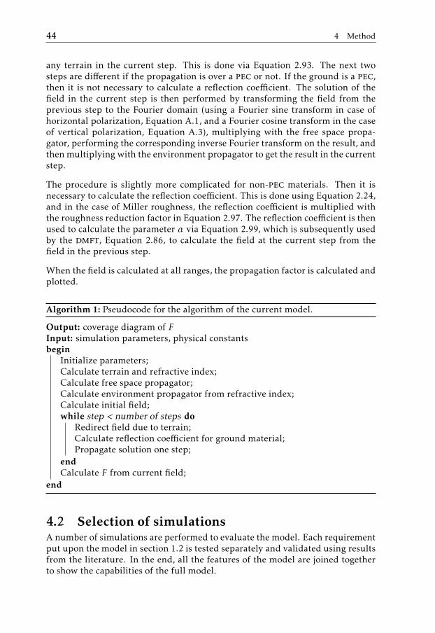
44 4 Method

any terrain in the current step. This is done via Equation 2.93. The next twosteps are different if the propagation is over a pec or not. If the ground is a pec,then it is not necessary to calculate a reflection coefficient. The solution of thefield in the current step is then performed by transforming the field from theprevious step to the Fourier domain (using a Fourier sine transform in case ofhorizontal polarization, Equation A.1, and a Fourier cosine transform in the caseof vertical polarization, Equation A.3), multiplying with the free space propa-gator, performing the corresponding inverse Fourier transform on the result, andthenmultiplying with the environment propagator to get the result in the currentstep.

The procedure is slightly more complicated for non-pec materials. Then it isnecessary to calculate the reflection coefficient. This is done using Equation 2.24,and in the case of Miller roughness, the reflection coefficient is multiplied withthe roughness reduction factor in Equation 2.97. The reflection coefficient is thenused to calculate the parameter α via Equation 2.99, which is subsequently usedby the dmft, Equation 2.86, to calculate the field at the current step from thefield in the previous step.

When the field is calculated at all ranges, the propagation factor is calculated andplotted.

Algorithm 1: Pseudocode for the algorithm of the current model.

Output: coverage diagram of FInput: simulation parameters, physical constantsbegin

Initialize parameters;Calculate terrain and refractive index;Calculate free space propagator;Calculate environment propagator from refractive index;Calculate initial field;while step < number of steps do

Redirect field due to terrain;Calculate reflection coefficient for ground material;Propagate solution one step;

endCalculate F from current field;

end

4.2 Selection of simulationsA number of simulations are performed to evaluate the model. Each requirementput upon the model in section 1.2 is tested separately and validated using resultsfrom the literature. In the end, all the features of the model are joined togetherto show the capabilities of the full model.

4.2 Selection of simulations 45

4.2.1 Numerical stabilityThe first test is to investigate the numerical stability of the model. This is donethrough simulation with decreasing steps in x-direction and then in z-direction.The simulation set-up is a simple one with propagation in vacuum over a pec sur-face. Two metrics are used to see how the results change for different simulationsteps. The first metric is calculated as

∆El =∑|ul |2∆zl −

∑|ul−1|2∆zl−1, (4.1)

where the quantity ∆E can be interpreted as related to the change in energy den-sity of the field with respect to the z-coordinate. The other metric is calculatedas

ϵl =

∑i |uil − u

il−1|

2∑|ul |2

, (4.2)

which can be seen as a normalized least squares error. The different calculationsteps in x are: 200–0.7813m, each time dividing the step by two, while the lengthstep in z is kept at 1/8m. For the case with varying z-step, the calculation stepsare 1/8–1/256m, each time halving the step, while the step in x is kept at 10m.

4.2.2 Free space propagationThis section deals with the simplest case in which we are interested in the result:free propagation. Free propagation in this case means propagation in vacuumover a flat, smooth surface that is supposed to be made of a pec. The comparisonis performed using the current model and the simulation tool petool [6]. Theyare both given the same simulation parameters. One simulation is performed forhorizontal polarization and one for vertical polarization. The simulation param-eters for the horizontal and vertical cases can be found in Table B.1.

4.2.3 Varying refractive indexThe next simulations deal with the case of a refractive index that is varying. Thecase of a varying refractive index is important in order tomodel a real atmosphereproperly. Three different cases are investigated here. One case in which the at-mosphere is taken to be a standard atmosphere. This case is compared to resultsobtained by Dockery [36]. The second case involves ducting conditions. The re-sults are compared against petool and the results by Gustafsson et al. [31], fromwhere the data for the duct is taken. The third case deals with absorption causedby precipitation.

The standard atmosphere is used to model both the actual atmosphere and thecurvature of the Earth. The results are compared with those presented by Dock-ery [36]. The aim is to reproduce Figure 2 in [36], so the simulation parametersused in the current model are taken from that article as far as possible. The exactsimulation parameters can be found in Table B.1.

It might be a bit hard to interpret the result and see the curvature of the Earthsince the x-axis follows the curvature of the Earth, which means that the coordi-nate system is not a Cartesian coordinate system. It is possible to do a coordinatetransform to convert the results to a Cartesian coordinate system, in which it is

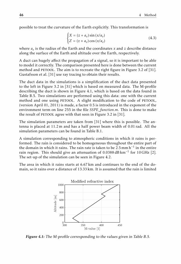
46 4 Method

possible to treat the curvature of the Earth explicitly. This transformation is⎧⎪⎪⎨⎪⎪⎩X = (z + ae) sin (x/ae)Z = (z + ae) cos (x/ae)

(4.3)

where ae is the radius of the Earth and the coordinates x and z describe distancealong the surface of the Earth and altitude over the Earth, respectively.

A duct can hugely affect the propagation of a signal, so it is important to be ableto model it correctly. The comparison presented here is done between the currentmethod and petool. The aim is to recreate the right figure in Figure 3.2 of [31].Gustafsson et al. [31] use ray tracing to obtain their results.

The duct data in the simulations is a simplification of the duct data presentedto the left in Figure 3.2 in [31] which is based on measured data. The M-profiledescribing the duct is shown in Figure 4.1, which is based on the data found inTable B.5. Two simulations are performed using this data: one with the currentmethod and one using petool. A slight modification to the code of petool,(version April 01, 2011) is made, a factor 0.5 is introduced in the exponent of theenvironment term on line 255 in the file SSPE_function.m. This is done to makethe result of petool agree with that seen in Figure 3.2 in [31].

The simulation parameters are taken from [31] where this is possible. The an-tenna is placed at 11.2m and has a half power beam width of 0.01 rad. All thesimulation parameters can be found in Table B.1.

A simulation corresponding to atmospheric conditions in which it rains is per-formed. The rain is considered to be homogeneous throughout the entire part ofthe domain in which it rains. The rain rate is taken to be 2.5mmh−1 in the entirerain region. This should give an attenuation of 0.0388dBkm−1 for 10GHz [2].The set-up of the simulation can be seen in Figure 4.2.

The area in which it rains starts at 6.67km and continues to the end of the do-main, so it rains over a distance of 13.33km. It is assumed that the rain is limited

300 350 400 4500

200

400

600

800

1000

Figure 4.1: The M-profile corresponding to the values given in Table B.5.

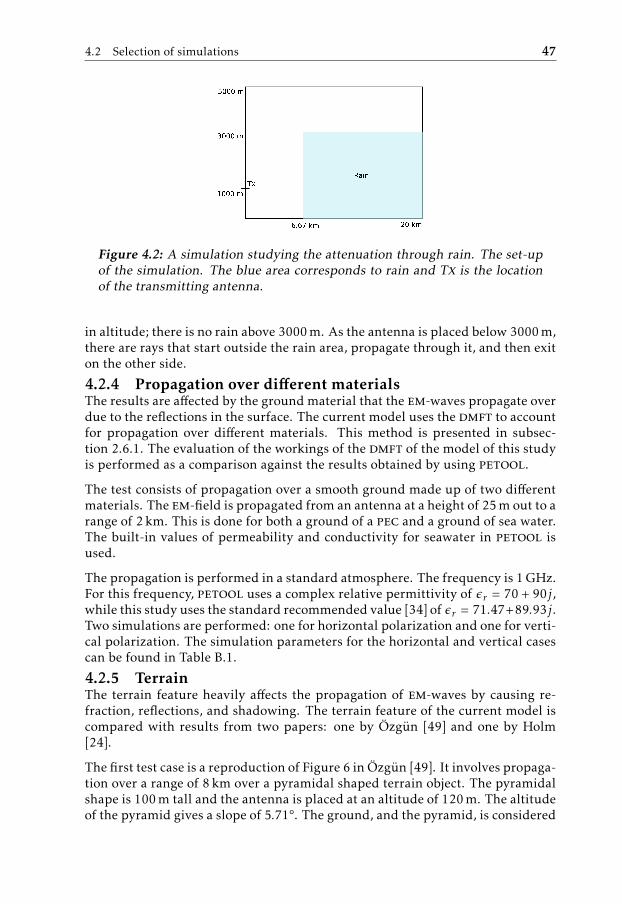
4.2 Selection of simulations 47

Figure 4.2: A simulation studying the attenuation through rain. The set-upof the simulation. The blue area corresponds to rain and Tx is the locationof the transmitting antenna.

in altitude; there is no rain above 3000m. As the antenna is placed below 3000m,there are rays that start outside the rain area, propagate through it, and then exiton the other side.

4.2.4 Propagation over different materialsThe results are affected by the ground material that the em-waves propagate overdue to the reflections in the surface. The current model uses the dmft to accountfor propagation over different materials. This method is presented in subsec-tion 2.6.1. The evaluation of the workings of the dmft of the model of this studyis performed as a comparison against the results obtained by using petool.

The test consists of propagation over a smooth ground made up of two differentmaterials. The em-field is propagated from an antenna at a height of 25m out to arange of 2 km. This is done for both a ground of a pec and a ground of sea water.The built-in values of permeability and conductivity for seawater in petool isused.

The propagation is performed in a standard atmosphere. The frequency is 1GHz.For this frequency, petool uses a complex relative permittivity of ϵr = 70 + 90j,while this study uses the standard recommended value [34] of ϵr = 71.47+89.93j.Two simulations are performed: one for horizontal polarization and one for verti-cal polarization. The simulation parameters for the horizontal and vertical casescan be found in Table B.1.

4.2.5 TerrainThe terrain feature heavily affects the propagation of em-waves by causing re-fraction, reflections, and shadowing. The terrain feature of the current model iscompared with results from two papers: one by Özgün [49] and one by Holm[24].

The first test case is a reproduction of Figure 6 in Özgün [49]. It involves propaga-tion over a range of 8 km over a pyramidal shaped terrain object. The pyramidalshape is 100m tall and the antenna is placed at an altitude of 120m. The altitudeof the pyramid gives a slope of 5.71°. The ground, and the pyramid, is considered

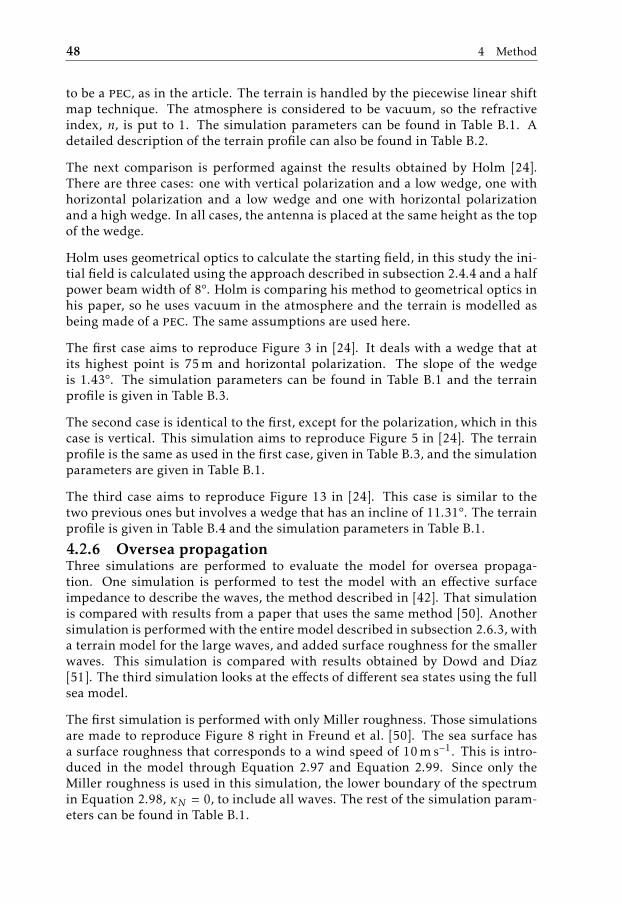
48 4 Method

to be a pec, as in the article. The terrain is handled by the piecewise linear shiftmap technique. The atmosphere is considered to be vacuum, so the refractiveindex, n, is put to 1. The simulation parameters can be found in Table B.1. Adetailed description of the terrain profile can also be found in Table B.2.

The next comparison is performed against the results obtained by Holm [24].There are three cases: one with vertical polarization and a low wedge, one withhorizontal polarization and a low wedge and one with horizontal polarizationand a high wedge. In all cases, the antenna is placed at the same height as the topof the wedge.

Holm uses geometrical optics to calculate the starting field, in this study the ini-tial field is calculated using the approach described in subsection 2.4.4 and a halfpower beam width of 8°. Holm is comparing his method to geometrical optics inhis paper, so he uses vacuum in the atmosphere and the terrain is modelled asbeing made of a pec. The same assumptions are used here.

The first case aims to reproduce Figure 3 in [24]. It deals with a wedge that atits highest point is 75m and horizontal polarization. The slope of the wedgeis 1.43°. The simulation parameters can be found in Table B.1 and the terrainprofile is given in Table B.3.

The second case is identical to the first, except for the polarization, which in thiscase is vertical. This simulation aims to reproduce Figure 5 in [24]. The terrainprofile is the same as used in the first case, given in Table B.3, and the simulationparameters are given in Table B.1.

The third case aims to reproduce Figure 13 in [24]. This case is similar to thetwo previous ones but involves a wedge that has an incline of 11.31°. The terrainprofile is given in Table B.4 and the simulation parameters in Table B.1.

4.2.6 Oversea propagationThree simulations are performed to evaluate the model for oversea propaga-tion. One simulation is performed to test the model with an effective surfaceimpedance to describe the waves, the method described in [42]. That simulationis compared with results from a paper that uses the same method [50]. Anothersimulation is performed with the entire model described in subsection 2.6.3, witha terrain model for the large waves, and added surface roughness for the smallerwaves. This simulation is compared with results obtained by Dowd and Díaz[51]. The third simulation looks at the effects of different sea states using the fullsea model.

The first simulation is performed with only Miller roughness. Those simulationsare made to reproduce Figure 8 right in Freund et al. [50]. The sea surface hasa surface roughness that corresponds to a wind speed of 10m s−1. This is intro-duced in the model through Equation 2.97 and Equation 2.99. Since only theMiller roughness is used in this simulation, the lower boundary of the spectrumin Equation 2.98, κN = 0, to include all waves. The rest of the simulation param-eters can be found in Table B.1.

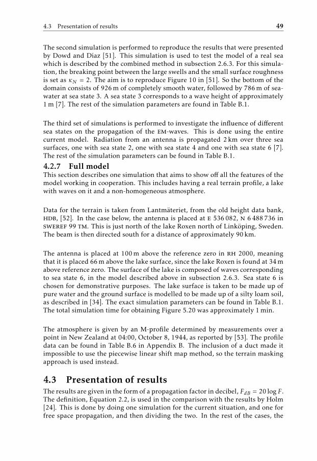
4.3 Presentation of results 49

The second simulation is performed to reproduce the results that were presentedby Dowd and Díaz [51]. This simulation is used to test the model of a real seawhich is described by the combined method in subsection 2.6.3. For this simula-tion, the breaking point between the large swells and the small surface roughnessis set as κN = 2. The aim is to reproduce Figure 10 in [51]. So the bottom of thedomain consists of 926m of completely smooth water, followed by 786m of sea-water at sea state 3. A sea state 3 corresponds to a wave height of approximately1m [7]. The rest of the simulation parameters are found in Table B.1.

The third set of simulations is performed to investigate the influence of differentsea states on the propagation of the em-waves. This is done using the entirecurrent model. Radiation from an antenna is propagated 2 km over three seasurfaces, one with sea state 2, one with sea state 4 and one with sea state 6 [7].The rest of the simulation parameters can be found in Table B.1.

4.2.7 Full modelThis section describes one simulation that aims to show off all the features of themodel working in cooperation. This includes having a real terrain profile, a lakewith waves on it and a non-homogeneous atmosphere.

Data for the terrain is taken from Lantmäteriet, from the old height data bank,hdb, [52]. In the case below, the antenna is placed at e 536 082, n 6 488 736 insweref 99 tm. This is just north of the lake Roxen north of Linköping, Sweden.The beam is then directed south for a distance of approximately 90 km.

The antenna is placed at 100m above the reference zero in rh 2000, meaningthat it is placed 66m above the lake surface, since the lake Roxen is found at 34mabove reference zero. The surface of the lake is composed of waves correspondingto sea state 6, in the model described above in subsection 2.6.3. Sea state 6 ischosen for demonstrative purposes. The lake surface is taken to be made up ofpure water and the ground surface is modelled to be made up of a silty loam soil,as described in [34]. The exact simulation parameters can be found in Table B.1.The total simulation time for obtaining Figure 5.20 was approximately 1min.

The atmosphere is given by an M-profile determined by measurements over apoint in New Zealand at 04:00, October 8, 1944, as reported by [53]. The profiledata can be found in Table B.6 in Appendix B. The inclusion of a duct made itimpossible to use the piecewise linear shift map method, so the terrain maskingapproach is used instead.

4.3 Presentation of resultsThe results are given in the form of a propagation factor in decibel, FdB = 20 log F.The definition, Equation 2.2, is used in the comparison with the results by Holm[24]. This is done by doing one simulation for the current situation, and one forfree space propagation, and then dividing the two. In the rest of the cases, the

50 4 Method

propagation factor is calculated using

F2 =LpLf p

= |u|2xλ, (4.4)

which is valid for the Earth-flattening transform in subsection 2.3.2. This expres-sion gives that F in decibel is

FdB = 10 log F2 = 20 log |u| + 10 log x + 10 logλ (4.5)

as it is given by Özgün et al. [6]. How the propagation factor in decibel is re-lated to the field strength through the path loss is derived by Levy [8], but sheunfortunately has a misprint in the final expression.

The comparisons against petool have been done with a locally installed version(version April 01, 2011) of petool [48] in matlab R2016b. Many results arealso compared against geometrical optics. It is not in the scope of this thesis todiscuss geometrical optics, and the reader that is not familiar with the subjectcan find [54] to be a good starting point.

5Results and discussion

This chapter presents data obtained using the method developed. The data ob-tained with the current model is compared with data that have been reported inthe literature. The results using the different features of the model are presentedand compared one by one. The different features dealt with here are free spacepropagation, varying refractive index, varying ground type, terrain and propaga-tion over a sea surface. The chapter ends with a general discussion of the validityof the current model, the choice of method and some possible sources of error.The method developed in this thesis is referred to as the current method below.

5.1 Numerical stabilityThe results from the simulations with varying ∆x can be seen in Figure 5.1. Theresult from the simulation with the maximum step length can be seen to the up-per left and the simulation with the minimum step length can be found to theupper right. The metric that is calculated using Equation 4.1 can be seen to thelower left and the metric that is calculated using Equation 4.2 can be seen to thelower right. It can be seen that the results in the top of the figure show the samegeneral behaviour, which is most clearly seen to the right in the simulation do-main. It can also be seen how both error metrics approach zero as the simulationstep decreases.

The results from the simulations with varying ∆z can be seen in Figure 5.2. Theresult from the simulation with the maximum step length can be seen to theupper left and the simulation with the minimum step length can be found to theupper right. The metric calculated using Equation 4.1 can be seen to the lowerleft and the metric calculated using Equation 4.2 can be seen to the lower right.It can be seen that the results in the top of the figure show the same general

51

52 5 Results and discussion

2 4 6 8 10

20

40

60

80

100

-50

-40

-30

-20

-10

0

10

2 4 6 8 10

20

40

60

80

100

-50

-40

-30

-20

-10

0

10

101 102 103 104-2.5

-2

-1.5

-1

-0.5

010-3

101 102 103 1040

0.05

0.1

0.15

Figure 5.1: Numerical stability with varying step in x. Upper left:Simulation result for ∆x = 200m. Upper right: Simulation result for∆x = 0.7813m. Lower left: Energy density as a function of the step length.Lower right: Normalised least squares error as function of the step length.

behaviour, which is most clearly seen to the right in the simulation domain. It isfound that both error metrics approach zero as the simulation step decreases.

The fact that both error metrics approach zero with decreasing calculation stepin both directions points to that the current method is numerically stable. Com-bining this with the fact that there is no qualitative difference in the behaviour ofthe solutions depending on the step length makes it possible to assume that themodel can be used with any of these resolutions. It is interesting to note that thereis a larger difference between the largest and smallest x-step than z-step. Thereis a larger range in x, but it comes from the fact that there is a maximum value of∆z from the Nyquist criteria, subsection 2.4.3. The maximum ∆z should captureall behaviour in z, so not much is gained by decreasing ∆z from the maximumone. This is clearly seen in the bottom right of Figure 5.2, where the normalizedmean square error is already on the order of half a per cent when stepping frommaximum ∆z to half of that.

5.2 Free space propagation 53

2 4 6 8 10

20

40

60

80

100

-50

-40

-30

-20

-10

0

10

2 4 6 8 10

20

40

60

80

100

-50

-40

-30

-20

-10

0

10

0.5 1 1.5 2 2.5

-8

-6

-4

-2

0

10-4

0.5 1 1.5 2 2.5

1

2

3

4

5

6

710-6

Figure 5.2: Numerical stability with varying step in z. Upper left: Simula-tion result for ∆z = 1/8m. Upper right: Simulation result for ∆z = 1/256m.Lower left: Energy density as a function of step length. Lower right: Nor-malised mean square error as function of step length.

5.2 Free space propagationThis section gives the results for the free space propagation simulations that arecompared with results obtained with petool [6].

The results for the case of horizontal polarization can be seen in Figure 5.3. To theleft is a coverage diagram that is obtained using the current method, and to theright is a comparison of the propagation factors that are obtained by the currentmethod and petool at a range of 10 km. It is clearly seen that the boundarycondition forces the field to be zero next to the ground, as it should be. Theantenna can clearly be seen on the left of the coverage diagram at an altitude of50m. The lobe pattern occurs due to destructive and constructive interferencecoming from difference in path length, since the rays that are reflected in theground must travel further than the rays that are travelling directly.

The results from this method and the ones from petool agree very well. Theminima vary somewhat in depth, but that is probably due to whether the grid

54 5 Results and discussion

2 4 6 8 10

20

40

60

80

100

-50

-40

-30

-20

-10

0

10

-50 -40 -30 -20 -10 0 100

20

40

60

80

100This studyPETOOL

Figure 5.3: Free space propagation for a field with horizontal polariza-tion. Left: Coverage diagram for free space propagation using the currentmethod. Right: Propagation factor versus altitude at range 10km for boththe current method and petool.

points are coinciding with the exact position of the minima or not. There is alsoa slight difference in lobe width between the two methods with petool havingslightly wider lobes. However, this is a very small difference.

The results for the case of vertical polarization can be seen in Figure 5.4. To theleft is a coverage diagram that is obtained using the current method, and to theright is a comparison of the propagation factors that are obtained by the currentmethod and petool at a range of 10 km. The only difference between this figureand Figure 5.3 is the polarization which requires a different boundary conditionnext to the ground. Here, the derivative of the field with respect to the altitude issupposed to be zero. This is fulfilled since the field interacts with the ground ata local maximum, which can clearly be seen to the right in Figure 5.4.

The agreement between the current model and petool is excellent in the caseof vertical polarization as well. The minima and maxima are at the exact samealtitudes. The small difference in lobe width that is seen in the case of horizontalpolarization is not seen here, so maybe it is an indication of a difference in theimplementation of the boundary conditions.

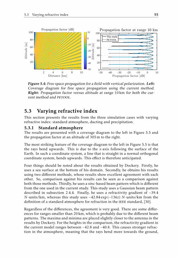
5.3 Varying refractive index 55

2 4 6 8 10

20

40

60

80

100

-50

-40

-30

-20

-10

0

10

-50 -40 -30 -20 -10 0 100

20

40

60

80

100This studyPETOOL

Figure 5.4: Free space propagation for a field with vertical polarization. Left:Coverage diagram for free space propagation using the current method.Right: Propagation factor versus altitude at range 10km for both the cur-rent method and petool.

5.3 Varying refractive indexThis section presents the results from the three simulation cases with varyingrefractive index: standard atmosphere, ducting and precipitation.

5.3.1 Standard atmosphereThe results are presented with a coverage diagram to the left in Figure 5.5 andthe propagation factor at an altitude of 305m to the right.

The most striking feature of the coverage diagram to the left in Figure 5.5 is thatthe rays bend upwards. This is due to the x-axis following the surface of theEarth. In such a coordinate system, a line that is straight in a normal orthogonalcoordinate system, bends upwards. This effect is therefore anticipated.

Four things should be noted about the results obtained by Dockery. Firstly, heuses a sea surface at the bottom of his domain. Secondly, he obtains his resultsusing two different methods, whose results show excellent agreement with eachother. So, comparison against his results can be seen as a comparison againstboth those methods. Thirdly, he uses a sinc-based beam pattern which is differentfrom the one used in the current study. This study uses a Gaussian beam patterndescribed in subsection 2.4.4. Finally, he uses a refractivity gradient of −39.4N -units/km, whereas this study uses −42.84 exp (−136z) N -units/km from thedefinition of a standard atmosphere for refraction in the ieee standard, [30].

Regardless of the differences, the agreement is very good. There are some differ-ences for ranges smaller than 20km, which is probably due to the different beampatterns. The maxima andminima are placed slightly closer to the antenna in theresults by Dockery. For the heights in the comparison, the refractivity gradient inthe current model ranges between −42.8 and −40.8. This causes stronger refrac-tion in the atmosphere, meaning that the rays bend more towards the ground,

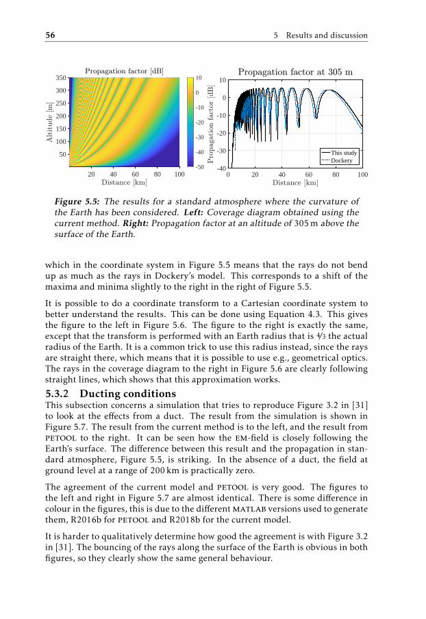
56 5 Results and discussion

20 40 60 80 100

50

100

150

200

250

300

350

-50

-40

-30

-20

-10

0

10

0 20 40 60 80 100-40

-30

-20

-10

0

10

This studyDockery

Figure 5.5: The results for a standard atmosphere where the curvature ofthe Earth has been considered. Left: Coverage diagram obtained using thecurrent method. Right: Propagation factor at an altitude of 305m above thesurface of the Earth.

which in the coordinate system in Figure 5.5 means that the rays do not bendup as much as the rays in Dockery’s model. This corresponds to a shift of themaxima and minima slightly to the right in the right of Figure 5.5.

It is possible to do a coordinate transform to a Cartesian coordinate system tobetter understand the results. This can be done using Equation 4.3. This givesthe figure to the left in Figure 5.6. The figure to the right is exactly the same,except that the transform is performed with an Earth radius that is 4/3 the actualradius of the Earth. It is a common trick to use this radius instead, since the raysare straight there, which means that it is possible to use e.g., geometrical optics.The rays in the coverage diagram to the right in Figure 5.6 are clearly followingstraight lines, which shows that this approximation works.

5.3.2 Ducting conditionsThis subsection concerns a simulation that tries to reproduce Figure 3.2 in [31]to look at the effects from a duct. The result from the simulation is shown inFigure 5.7. The result from the current method is to the left, and the result frompetool to the right. It can be seen how the em-field is closely following theEarth’s surface. The difference between this result and the propagation in stan-dard atmosphere, Figure 5.5, is striking. In the absence of a duct, the field atground level at a range of 200 km is practically zero.

The agreement of the current model and petool is very good. The figures tothe left and right in Figure 5.7 are almost identical. There is some difference incolour in the figures, this is due to the differentmatlab versions used to generatethem, R2016b for petool and R2018b for the current model.

It is harder to qualitatively determine how good the agreement is with Figure 3.2in [31]. The bouncing of the rays along the surface of the Earth is obvious in bothfigures, so they clearly show the same general behaviour.

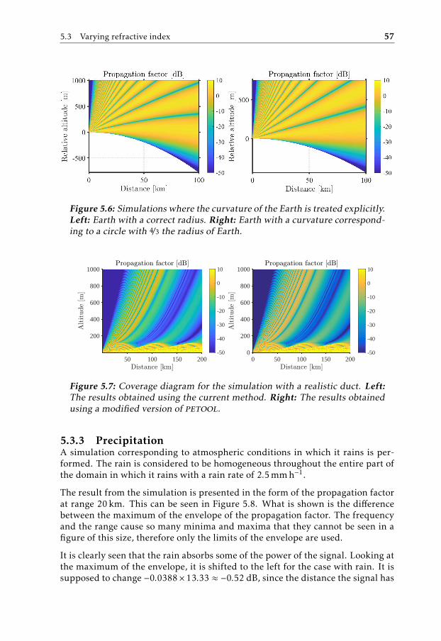
5.3 Varying refractive index 57

Figure 5.6: Simulations where the curvature of the Earth is treated explicitly.Left: Earth with a correct radius. Right: Earth with a curvature correspond-ing to a circle with 4/3 the radius of Earth.

50 100 150 200

200

400

600

800

1000

-50

-40

-30

-20

-10

0

10

0 50 100 150 2000

200

400

600

800

1000

-50

-40

-30

-20

-10

0

10

Figure 5.7: Coverage diagram for the simulation with a realistic duct. Left:The results obtained using the current method. Right: The results obtainedusing a modified version of petool.

5.3.3 PrecipitationA simulation corresponding to atmospheric conditions in which it rains is per-formed. The rain is considered to be homogeneous throughout the entire part ofthe domain in which it rains with a rain rate of 2.5mmh−1.

The result from the simulation is presented in the form of the propagation factorat range 20 km. This can be seen in Figure 5.8. What is shown is the differencebetween the maximum of the envelope of the propagation factor. The frequencyand the range cause so many minima and maxima that they cannot be seen in afigure of this size, therefore only the limits of the envelope are used.

It is clearly seen that the rain absorbs some of the power of the signal. Looking atthe maximum of the envelope, it is shifted to the left for the case with rain. It issupposed to change −0.0388× 13.33 ≈ −0.52 dB, since the distance the signal has

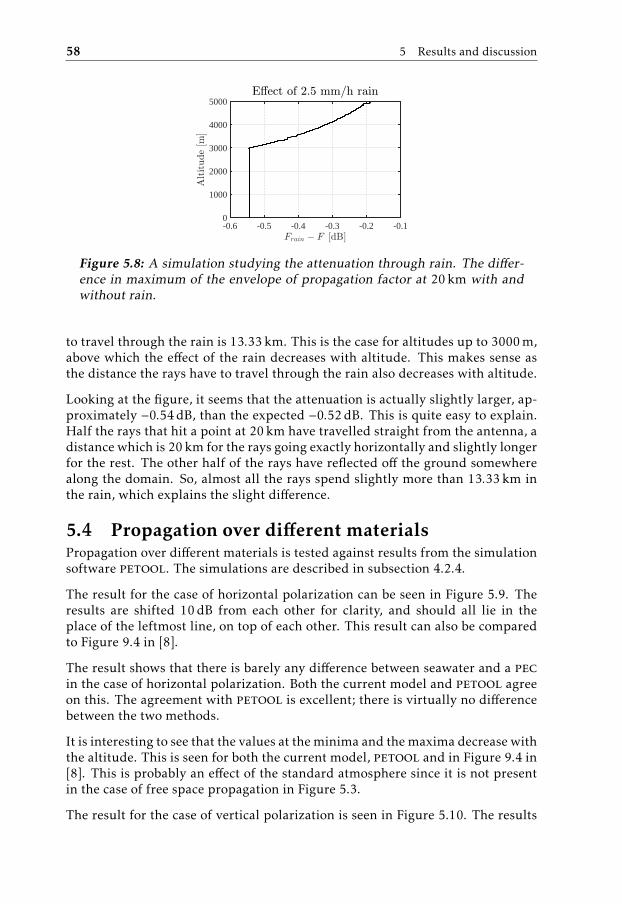
58 5 Results and discussion

-0.6 -0.5 -0.4 -0.3 -0.2 -0.10

1000

2000

3000

4000

5000

Figure 5.8: A simulation studying the attenuation through rain. The differ-ence in maximum of the envelope of propagation factor at 20km with andwithout rain.

to travel through the rain is 13.33km. This is the case for altitudes up to 3000m,above which the effect of the rain decreases with altitude. This makes sense asthe distance the rays have to travel through the rain also decreases with altitude.

Looking at the figure, it seems that the attenuation is actually slightly larger, ap-proximately −0.54dB, than the expected −0.52dB. This is quite easy to explain.Half the rays that hit a point at 20 km have travelled straight from the antenna, adistance which is 20 km for the rays going exactly horizontally and slightly longerfor the rest. The other half of the rays have reflected off the ground somewherealong the domain. So, almost all the rays spend slightly more than 13.33km inthe rain, which explains the slight difference.

5.4 Propagation over different materialsPropagation over different materials is tested against results from the simulationsoftware petool. The simulations are described in subsection 4.2.4.

The result for the case of horizontal polarization can be seen in Figure 5.9. Theresults are shifted 10dB from each other for clarity, and should all lie in theplace of the leftmost line, on top of each other. This result can also be comparedto Figure 9.4 in [8].

The result shows that there is barely any difference between seawater and a pecin the case of horizontal polarization. Both the current model and petool agreeon this. The agreement with petool is excellent; there is virtually no differencebetween the two methods.

It is interesting to see that the values at theminima and themaxima decrease withthe altitude. This is seen for both the current model, petool and in Figure 9.4 in[8]. This is probably an effect of the standard atmosphere since it is not presentin the case of free space propagation in Figure 5.3.

The result for the case of vertical polarization is seen in Figure 5.10. The results

5.4 Propagation over different materials 59

-40 -30 -20 -10 0 10 20 30 400

20

40

60

80

100PEC current mod.PEC PETOOLSea current mod.Sea PETOOL

Figure 5.9: Propagation factors for this study and petool at 2000m in stan-dard atmosphere with horizontal polarization. The results are shifted 10dBfrom each other for clarity.

from this study are shifted 30dB for clarity. So, all results should lie in the placeof the results from petool. This result can also be compared to Figure 9.4 in [8].

There is a difference between seawater and pec in the case of vertical polariza-tion, as can be seen in Figure 5.10. The minima and maxima are much smaller inthe case of seawater than a pec. This is the case both the for current model andpetool. This is also seen in Figure 9.4 in [8].

There are two small differences between the current method and petool for the

-40 -30 -20 -10 0 10 20 30 400

20

40

60

80

100PEC current mod.PEC PETOOLSea current mod.Sea PETOOL

Figure 5.10: Propagation factors for this study and petool at 2000m instandard atmosphere with vertical polarization. The results from this studyare shifted 30dB for clarity.

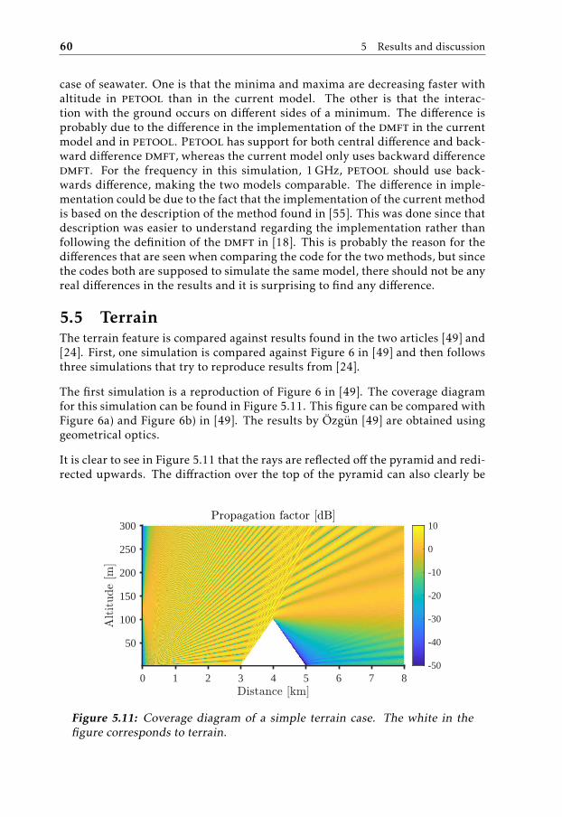
60 5 Results and discussion

case of seawater. One is that the minima and maxima are decreasing faster withaltitude in petool than in the current model. The other is that the interac-tion with the ground occurs on different sides of a minimum. The difference isprobably due to the difference in the implementation of the dmft in the currentmodel and in petool. Petool has support for both central difference and back-ward difference dmft, whereas the current model only uses backward differencedmft. For the frequency in this simulation, 1GHz, petool should use back-wards difference, making the two models comparable. The difference in imple-mentation could be due to the fact that the implementation of the current methodis based on the description of the method found in [55]. This was done since thatdescription was easier to understand regarding the implementation rather thanfollowing the definition of the dmft in [18]. This is probably the reason for thedifferences that are seen when comparing the code for the two methods, but sincethe codes both are supposed to simulate the same model, there should not be anyreal differences in the results and it is surprising to find any difference.

5.5 TerrainThe terrain feature is compared against results found in the two articles [49] and[24]. First, one simulation is compared against Figure 6 in [49] and then followsthree simulations that try to reproduce results from [24].

The first simulation is a reproduction of Figure 6 in [49]. The coverage diagramfor this simulation can be found in Figure 5.11. This figure can be compared withFigure 6a) and Figure 6b) in [49]. The results by Özgün [49] are obtained usinggeometrical optics.

It is clear to see in Figure 5.11 that the rays are reflected off the pyramid and redi-rected upwards. The diffraction over the top of the pyramid can also clearly be

0 1 2 3 4 5 6 7 8

50

100

150

200

250

300

-50

-40

-30

-20

-10

0

10

Figure 5.11: Coverage diagram of a simple terrain case. The white in thefigure corresponds to terrain.

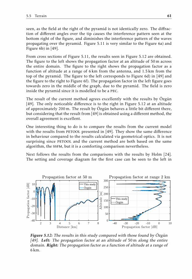
5.5 Terrain 61

seen, as the field at the right of the pyramid is not identically zero. The diffrac-tion of different angles over the tip causes the interference pattern seen at thebottom right of the figure, and diminishes the interference pattern of the wavespropagating over the pyramid. Figure 5.11 is very similar to the Figure 6a) andFigure 6b) in [49].

From cross sections of Figure 5.11, the results seen in Figure 5.12 are obtained.The figure to the left shows the propagation factor at an altitude of 50m acrossthe entire domain. The figure to the right shows the propagation factor as afunction of altitude at a range of 6 km from the antenna, and 1.5km from thetop of the pyramid. The figure to the left corresponds to Figure 6d) in [49] andthe figure to the right to Figure 6f). The propagation factor in the left figure goestowards zero in the middle of the graph, due to the pyramid. The field is zeroinside the pyramid since it is modelled to be a pec.

The result of the current method agrees excellently with the results by Özgün[49]. The only noticeable difference is to the right in Figure 5.12 at an altitudeof approximately 200m. The result by Özgün behaves a little bit different there,but considering that the result from [49] is obtained using a different method, theoverall agreement is excellent.

One interesting thing to do is to compare the results from the current modelwith the results from petool presented in [49]. They show the same differencein behaviour compared to the results calculated via geometrical optics. It is notsurprising since petool and the current method are both based on the samealgorithm, the ssfm, but it is a comforting comparison nevertheless.

Next follows the results from the comparisons with the results by Holm [24].The setting and coverage diagram for the first case can be seen to the left in

2 3 4 5 6 7 8-40

-30

-20

-10

0

10 This studyÖzgün

-40 -30 -20 -10 0 100

50

100

150

200

250

300

This studyÖzgün

Figure 5.12: The results in this study compared with those found by Özgün[49]. Left: The propagation factor at an altitude of 50m along the entiredomain. Right: The propagation factor as a function of altitude at a range of6km.

62 5 Results and discussion

Figure 5.13. The antenna is placed to the left outside of the figure, at distance 0.The wedge in the centre of the figure has an angle of incline of 1.43°. It is clearto see how the wedge in the middle of the figure affects the interference pattern.However, the strong reflections against the wedge that are present in Figure 5.12are not present here. This is because the wedge is shadowed by the terrain closerto the antenna from the rays reflected off the ground.

The propagation factor at the end of the terrain profile, at 10 km is given to theright in Figure 5.13. The agreement with the results by Holm [24] is excellent.Here, in the right of Figure 5.13, it is possible to see how the rightmost verticalprofile of the propagation factor varies in the coverage diagram to the left inFigure 5.13.

The second case, shown in Figure 5.14, corresponds to vertical polarization withthe same, small wedge as in the first case. The coverage diagram can be found tothe left in the figure. To the right is the propagation factor versus altitude at thefar right of the domain. The set-up is similar to Figure 5 in [24] so the coveragediagram to the left in Figure 5.14 can be compared to that figure.

Comparing the results with Holm [24], there is an excellent agreement. Both forthe coverage diagram, left in Figure 5.14 and Figure 5 in [24] and the propagationfactor at the end of the domain, right in Figure 5.14. The current model capturesthe behaviour of the em-field in the same way as Holm’s model.

There is a clear difference between Figure 5.13 and Figure 5.14, between horizon-tal and vertical polarization. It can be seen in Figure 5.14 how the field followsthe terrain profile in the vertical case due to it having a maximum at the lowerboundary. This causes stronger diffraction around the edges of the terrain. The

2.5 4 6 8 100

50

100

150

200

-40

-30

-20

-10

0

10

0 50 100 150 200-60

-50

-40

-30

-20

-10

0

10

This studyHolm

Figure 5.13: Comparison of the results from this study with the results ob-tained by Holm [24]. These results correspond to horizontal polarization.Left: Coverage diagram over the entire domain using the method developedin this study. The white parts correspond to terrain. Right: The propagationfactor versus altitude at a distance of 10km.

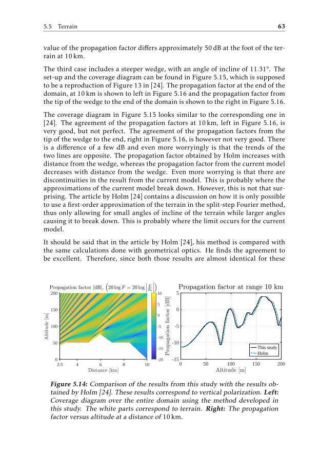
5.5 Terrain 63

value of the propagation factor differs approximately 50dB at the foot of the ter-rain at 10 km.

The third case includes a steeper wedge, with an angle of incline of 11.31°. Theset-up and the coverage diagram can be found in Figure 5.15, which is supposedto be a reproduction of Figure 13 in [24]. The propagation factor at the end of thedomain, at 10 km is shown to left in Figure 5.16 and the propagation factor fromthe tip of the wedge to the end of the domain is shown to the right in Figure 5.16.

The coverage diagram in Figure 5.15 looks similar to the corresponding one in[24]. The agreement of the propagation factors at 10 km, left in Figure 5.16, isvery good, but not perfect. The agreement of the propagation factors from thetip of the wedge to the end, right in Figure 5.16, is however not very good. Thereis a difference of a few dB and even more worryingly is that the trends of thetwo lines are opposite. The propagation factor obtained by Holm increases withdistance from the wedge, whereas the propagation factor from the current modeldecreases with distance from the wedge. Even more worrying is that there arediscontinuities in the result from the current model. This is probably where theapproximations of the current model break down. However, this is not that sur-prising. The article by Holm [24] contains a discussion on how it is only possibleto use a first-order approximation of the terrain in the split-step Fourier method,thus only allowing for small angles of incline of the terrain while larger anglescausing it to break down. This is probably where the limit occurs for the currentmodel.

It should be said that in the article by Holm [24], his method is compared withthe same calculations done with geometrical optics. He finds the agreement tobe excellent. Therefore, since both those results are almost identical for these

2.5 4 6 8 100

50

100

150

200

-20

-15

-10

-5

0

5

10

0 50 100 150 200-15

-10

-5

0

5

This studyHolm

Figure 5.14: Comparison of the results from this study with the results ob-tained by Holm [24]. These results correspond to vertical polarization. Left:Coverage diagram over the entire domain using the method developed inthis study. The white parts correspond to terrain. Right: The propagationfactor versus altitude at a distance of 10km.

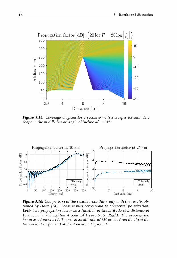
64 5 Results and discussion

2.5 4 6 8 100

50

100

150

200

250

300

350

-40

-30

-20

-10

0

10

Figure 5.15: Coverage diagram for a scenario with a steeper terrain. Theshape in the middle has an angle of incline of 11.31°.

0 50 100 150 200 250 300 350

-40

-30

-20

-10

0

This studyHolm

6 7 8 9 10-10

-8

-6

-4

-2

This studyHolm

Figure 5.16: Comparison of the results from this study with the results ob-tained by Holm [24]. These results correspond to horizontal polarization.Left: The propagation factor as a function of the altitude at a distance of10km, i.e. at the rightmost point of Figure 5.15. Right: The propagationfactor as a function of distance at an altitude of 250m, i.e. from the tip of theterrain to the right end of the domain in Figure 5.15.

5.6 Oversea propagation 65

scenarios, the comparison done here against the results in [24] is valid as a com-parison against both his method and the geometrical optics calculations. Thus,the current model can be said to also agree well with geometrical optics for anglesof incline smaller than 10°.

5.6 Oversea propagationThis section deals with the case of oversea propagation. Three sets of simulationsare performed: one concerning effective impedance of a sea surface that is com-pared with results by Freund et al. [50], one with the entire sea surface modelthat is compared with results from Dowd and Díaz [51] and one that looks athow different sea states affect the propagation using the entire sea surface modeldescribed in subsection 2.6.3. The simulations are described in subsection 4.2.6.

The results from the first set of simulations are shown in Figure 5.17. The cov-erage diagram can be seen to the left and the propagation factors at a distance of5 km to the right. It is clearly seen in the coverage diagram to the left how thesurface roughness of the surface reduces the interference pattern with minimaand maxima.

The agreement with the results by Freund et al. [50] is very good. Both resultsshow how both the minima and maxima decrease with altitude. This is expected,since Equation 2.97 gives that the roughness reduction factor decreases with in-creasing grazing angle through ξ. This causes the effective reflection coefficientR = ρR0 to decrease with altitude. The difference between the case of a smoothsea and a rough sea is clear. It can be seen in Figure 5.17 that the maximum de-crease, and the minimum values increase with altitude in the case of a rough sea.For a smooth sea, they do not. The current model has stronger minima and max-ima than the results by Freund et al. This might be due to the use of a differentsea spectrum in [50].

The second simulation uses the entire sea surface model. The results from thissimulation are shown in Figure 5.18, with a coverage diagram to the left and acomparison of the different propagation factors at a distance of 1650m to theright. It is possible to see the terrain representation of the sea surface on thebottom of the coverage diagram on the left.

The agreement with Dowd and Díaz [51] is in general good. The comparison ismade harder by the fact that the ocean surface is generated by a random process.However, the maxima and minima should still be at the same height, which theyare not. The maxima are shifted slightly up for the results by Dowd and Díaz.This might be due to some difference in atmosphere used, since it was not veryclear from [51] what kind of atmosphere that was used.

The results from the simulations looking at the effects of the different sea statesare seen in Figure 5.19. It is clear that the sea state has a large effect on thepropagation. It should be noted that the sea state is not linearly dependent on thewave size, but rather on the square root of the average sea height [7]. Sea state 2,upper left in Figure 5.19, is quite similar to propagation over a smooth surface.

66 5 Results and discussion

1 2 3 4 5

50

100

150

-50

-40

-30

-20

-10

0

10

-20 -15 -10 -5 0 50

50

100

150RoughFreund et al.Smooth

Figure 5.17: Comparison of the results from using the current model andthe results obtained by Freund et al. [50] for a wind of 10ms−1. Left: Cov-erage diagram obtained using the current method. Right: Comparison ofthe propagation factors at a distance of 5km. A line giving the propagationfactor for a smooth sea is also included.

1 1.2 1.4 1.6

0

5

10

15

-10

-5

0

5

10

-15 -10 -5 0 5 100

5

10

15This studyDowd et al.

Figure 5.18: Comparison of the results from using the current model and theresults obtained by Dowd and Díaz [51]. Left: Coverage diagram obtainedusing the current method. Right: Comparison of the propagation factors ata distance of 1650m.

5.6 Oversea propagation 67

But that is not very surprising when seeing how small the waves are in the figure.The sea waves aremuch larger in the case of sea state 4, upper right in Figure 5.19,and the influence on the propagation of the em-waves is greater. Interferencein the coverage pattern for the figure for sea state 4, due to reflection off thewaves can clearly be seen. The effect from the sea waves at sea state 6, lowerleft in Figure 5.19, is greater still. It is even possible to see how one of the lobesdisappears among the waves around range 0.5km. An overview of these effectscan be obtained by looking at the propagation factors at a range of 2 km for thethree sea states, lower right in Figure 5.19. The propagation factor for sea state2 has almost the same kind of interference pattern as that for a perfectly smoothsea, Figure 5.9 above. That pattern is somewhat distorted for sea state 4, withlower maxima and higher minima. The pattern for sea state 6 is very different.There are still maxima and minima but they are not at the same altitudes anymore.

0.5 1 1.5 2

0

5

10

15

20

-50

-40

-30

-20

-10

0

10

0.5 1 1.5 2

0

5

10

15

20

-50

-40

-30

-20

-10

0

10

-30 -20 -10 0 100

5

10

15

20

25

Sea State 2Sea State 4Sea State 6

Figure 5.19: Simulations of different sea states. Upper left: Situation corre-sponding to sea state 2. Upper right: Situation corresponding to sea state 4.Lower left: Situation corresponding to sea state 6. Lower right: Propagationfactors as function of altitude for the different sea states.

68 5 Results and discussion

5.7 Full modelThe results from the simulation made with the full model are seen in Figure 5.20.The lake surface can be seen in the bottom left of the figure, where it is possibleto see the small roughness that corresponds to the waves. Even though the lakeis at sea state 6, which corresponds to a wave height of 4–6 meters [7], it is hardto see at this scale in altitude.

The duct can clearly be seen between the ranges 10–40 km and around an altitudeof 150m. It is seen that the duct causes the hill at 40 km to be lit by the radiationfurther down than what can be considered to be line-of-sight from the antenna.The presence of the duct will clearly affect the performance of the radar, had thisbeen an actual set-up. Since radar is two-way propagation, it is interesting to seehow the reflections off the hill in question propagates back to the antenna. Thisis the intent of Figure 5.21.

Figure 5.21 was constructed by placing an imaginary antenna at the side of thehill at 40 km in Figure 5.20 and then turning the terrain the other way aroundso that the em-waves propagate in the other direction. It can be seen in the fig-ure how the reflected waves interfere into two maxima in the lower right of thefigure, with one at an altitude of 100m, the altitude of the transmitting antenna.This is not very surprising since the same effects should affect the propagation inboth directions. The approximation to just square the propagation factor to ac-count for two-way propagation, that is mentioned in section 2.1, therefore seemsreasonable from this simple example.

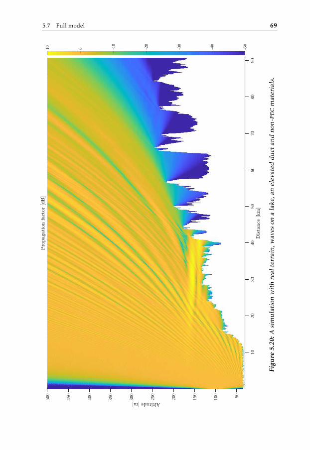
5.7 Full model 69

1020

3040

5060

7080

90

50100

150

200

250

300

350

400

450

500

-50

-40

-30

-20

-10

010

Figu

re5.20

:Asimulationwithreal

terrain,

waves

onalake

,anelevated

duct

andno

n-pecmaterials.

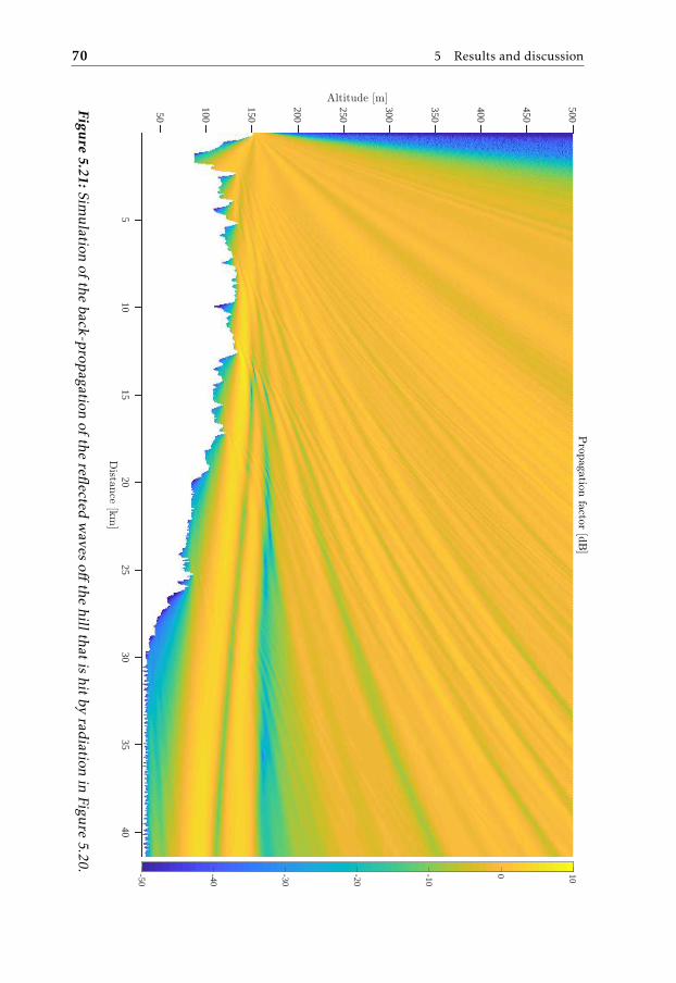
70 5 Results and discussion

510

1520

2530

3540

50

100

150

200

250

300

350

400

450

500

-50

-40

-30

-20

-10

0 10

Figure

5.21:Simulation

ofthe

back-propagationof

therefl

ectedwaves

offthe

hillthatishit

byradiation

inFigure

5.20.

5.8 Method 71

5.8 MethodThe initial choice to use the split-step Fourier method seems to have been a goodone. All features that were requested could be introduced inside the scope of themodel. However, it is not entirely without difficulties in some cases.

The main problem of the method is the handling of non-pec materials for theground. This can be solved by using a method like the dmft, despite it being amethod that is not very intuitive. It also has the problem of being quite slow. Oneof the main reasons for choosing ssfm is its speed, and using the dmft algorithmsomewhat reduces that advantage.

The method of choice for handling terrain, the piecewise linear shift map, worksby redirecting the field towards the ground with the same angle that the terrainrises with. The steering of the beam makes it hard to combine this method witha varying refractive index of the atmosphere. For example, a duct works like awaveguide and is highly dependent on the angle of arrival of the wave into theduct. Steering the field up and down, by following the underlying terrain, leadsto unrealistic results. The author is not aware of anyone that has successfullycombined the piecewise linear shift map with ducts. It is possible to use theterrain masking approach to account for the terrain at the same time when usinga non-homogeneous atmosphere. However, this is a method that does not give asgood results as the piecewise linear shift map [37].

The method for describing the sea surface does seem like an intuitively good one.The choice to use a terrain-like profile to describe the waves makes it possibleto include shadowing on part of the waves and reflections off part of the waves.This should give a result that is more realistic, since those effects can appearin reality. What can be said is that the result from using such an approach isvery different from using an effective reflection coefficient as in Figure 5.17. Itseems intuitively correct that a very uneven surface should give a different in-terference pattern compared to an even surface. The problem with the currentmethod for sea waves is the same as for the terrain, the problem is to combineit with a ducting atmosphere due to the limitation of using the piecewise linearshift map. The importance of the problem increases with increasing sea state asthe waves get larger, and also the slopes of the waves. However, the presenceof such strong winds, like those causing the waves, will probably mix the atmo-sphere, thereby making an evaporation duct less pronounced. On the other hand,there will probably be a lot of spray from the waves in the atmosphere which canchange the propagation environment. The main thread of reasoning here is thatthe limitation of not being able to have a duct combined with very large wavesmight not be a problem for simulation of realistic environments.

5.9 Sources of errorThere are several sources of error that are introduced in the approximations lead-ing up to the parabolic equation and the split-step Fourier method. These havebeen discussed by others, e.g. [8, 15], and found to be reasonably small for prac-

72 5 Results and discussion

tical purposes. This section will deal with the errors introduced in the currentimplementation of the split-step Fourier method.

One obvious source of error is the truncation of the domain in the positive z-direction. As this is done through a dampening window, reflections cannot beruled out. This would mean that signals reflected from the top of the calculationdomain would interfere with the field in the domain of interest. The dampeningthat the signal undergoes inside the window is dependent of the distance it trav-els inside the influence of the window function. The distance travelled dependson the propagation angle of the wave. A lower angle leads to a longer distanceand thus a stronger dampening. In a domain with a flat ground, this angle is onlya few degrees. The introduction of terrain in the domain increases this angle sig-nificantly, since reflected signals will have a propagation angle that is twice theangle of slope of the terrain. It is therefore easy to use too small a truncationwindow when terrain is present. This could alternatively have been solved by theimplementation of a perfectly matching layer as described in [8, 24].

One other source of error is that using this method, a 3d environment is ap-proximated using a 2d slice. This means that any refraction taking place in thexy plane will be omitted. In the environments considered, this could be wavesthat travel around an island rather than over it. It is unclear how large the errorcaused by this is. But considering that a radar system usually rotates, lookingin one direction at a time, the approximation is maybe closer to reality than onemight think.

6Conclusions

This chapter concludes the thesis. The fulfilment of the aims of section 1.2 arediscussed in view of the results obtained. The chapter ends with some sugges-tions of further studies which could be the subject of further research.

6.1 ConclusionsThis thesis has set out to develop a model that describes electromagnetic propa-gation in a realistic environment, as described in section 1.2 as an environment,with a varying refractive index, terrain, and a sea surface. The model was de-veloped using a parabolic equation approach together with the split-step Fouriermethod, ssfm. Each feature of the model has been presented and verified inchapter 5, through the comparison with numerical software developed by others.The results obtained using the current method agrees well with similar resultsfound in the literature.

The validity was tested in chapter 5, and good agreement was shown for most ofthe test cases, such as non-homogeneous atmosphere, propagation over a smoothsurface and lossy ground. The only test case in which the current model fails togive a good result is for terrain features with steep slopes, having an inclinationof more than 10°. The current model shows discontinuities for such a case. How-ever, this was not very surprising since it is known that the method chosen forthe implementation of the terrain, the piecewise linear shift map, is limited inhow steep angles that it can correctly describe. For the case of a gentler slope,the current model gives results that agree well with previous results, obtained bygeometrical optics, that are found in the literature.

As the current model has been compared with results obtained by completelydifferent methods in chapter 5, such as geometrical optics and ray tracing, the

73

74 6 Conclusions

validity of the results can also be seen as a validation of the entire pe approachusing the ssfm. So, it can be said from looking at the results in chapter 5 that thechoice of the pe together with the ssfm was a good one. It is a suitable methodfor modelling radar propagation with good result. Some approximations seemquite rough during the derivation of the equations, but the result shows that theyare reasonable approximations for the situation considered.

There are two results that are of special interest. The first one is how different seastates influences the em-propagation above an ocean surface. It is clear that thesea state heavily influences the field that propagates over the sea, especially forhigher sea states. It can also be seen how the common approximation of a sea sur-face as a smooth perfect electric conductor can be valid for a low sea state, up tosea state 3, but not further. This analysis was made possible by the ocean modelused in the current study. The sea surface was modelled as a combination of ter-rain for large sea swells, and Miller surface roughness for smaller waves. Theheight profile of the waves was randomly generated from a Pierson-Moskowitzsea spectrum, as was the Miller surface roughness. The large swells were handledusing the piecewise linear shift map technique which allows for good reflectionsoff the large waves. A similar approach was previously presented in [38], butthe current model should, in theory, give more realistic results due to the moreadvanced terrain model. However, the piecewise linear shift map is hard to com-bine with a non-homogeneous atmosphere due to its steering of the beam, whichmeans that it is difficult to combine large waves with an evaporation duct in thecurrent model. However, as sea waves are mostly wind-driven, it is unlikely thata distinct evaporation duct should be present in the case of a high sea state.

The other especially interesting result was the simulation in which all the featuresof the model work are included. Here the simulation was performed with a non-homogeneous atmosphere over a realistic terrain that included a lake that wasmade up of, different, lossy materials. The result showed that even though thepropagation of the em-waves is hindered by terrain; the situation can drasticallychange in the presence of a duct. So, in order to simulate a situation that aims tomimic the reality, it is important to include as many features as possible.

6.2 Future workIn the course of the current work some ideas have emerged that would be inter-esting to look into more closely. Some of them are presented here.

• Reciprocity: It would be interesting to look at a model that can correctlyinclude em-waves that are propagating in another direction than along thex-axis. This would allow for more reflection effects and interference fromwaves that are travelling in different directions. Such a model could an-swer the question if it is correct to square the propagation factor to get thebehaviour of two-way propagation. The parabolic equation approach doesnot directly allow for this, so another approach is necessary.

• Terrain: The kind of terrain that can be modelled to an acceptable degree

6.2 Future work 75

with the current model is very limited due to the restriction that the slopehas to be smaller than approximately 10°. There is a lot of real terrain that isexcluded by this requirement. This limit has to be increased greatly to allowinvestigation of arbitrary terrain anywhere. It would also be interesting ifthe terrain model could be used inside a duct.

• Target modelling: The idea is to use the current model for radar appli-cations. Since a radar listens for the echo off the target it is necessary toinclude a model for how the signal is reflected off the target to get a morerealistic model. This could for example be done by ray tracing close to thetarget, and ssfm for the propagation over the long ranges. This would, how-ever, require that the model used allows for propagation far off the paraxialdirection.

• Radical splitting: One more mathematical point of interest for furtherstudy, pointed out by P. Holm, is the splitting of the radical in Equation 2.89.This is currently done as a first order approximation. Finding a more accu-rate approximation of the radical would lead to a better approximation ofthe terrain profile, something that should lead to a less severe restriction ofthe slope of the profile.

• Radar system: It would be interesting to include some more specific pa-rameters of a radar system into the model. This would enable the user toinvestigate how the choice of system affects the propagation. One examplecould be the choice to use a pulsed radar. For such a system, the outgo-ing signal would have a limited chance to interact with itself. This meansthat the results for reflection off a surface would be different, given that thecurrent model assumes the possibility of interference.

Appendices

77

ATransforms

This appendix contains the definitions used for the different kinds of Fouriertransforms used in this report.

A.1 Sine transformThe sine transform used is the same as in [22], which is defined as

Su(x, z) =∞∫0

u(x, z) sin pzz dz. (A.1)

The inverse transform is then

S−1u(x, pz) =2π

∞∫0

u(x, pz) sin pzz dpz . (A.2)

A.2 Cosine transformThe cosine transform used is the same as in [22], which is defined as

Cu(x, z) =∞∫0

u(x, z) cos pzz dz. (A.3)

The inverse transform is then

C−1u(x, pz) =2π

∞∫0

u(x, pz) cos pzz dpz . (A.4)

79

80 A Transforms

A.3 Mixed Fourier transformThe mixed Fourier transform was first introduced by Kuttler and Dockery [18]in order to be able to have impedance boundary conditions. The mixed Fouriertransform is defined in their paper as

u(x, pz) =

∞∫0

u(x, z) [α sin pzz − pz cos pzz] dz (A.5)

where α is a parameter related to the complex relative permittivity, ϵr , of theground.

BSimulation parameters

This appendix contains the most important simulation parameters for the figurespresented in chapter 5. First follows a table containing the simulation parametersfor all figures, then follows the terrain profiles for the simpler terrains, and in theend atmospheric data is given for the cases of non-standard atmospheres.

81

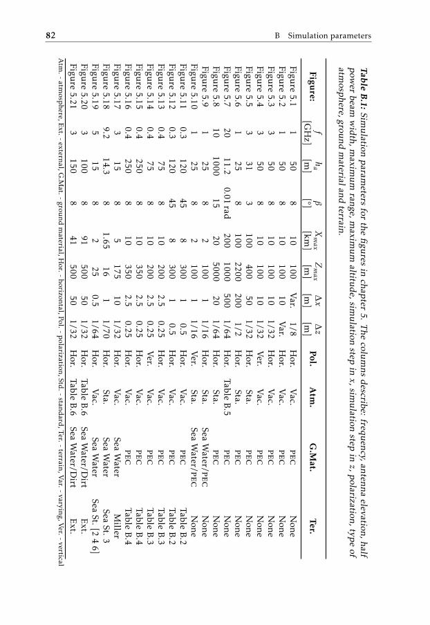
82 B Simulation parameters

TableB.1:

Simulation

parameters

forthe

figures

inchapter

5.The

columns

describe:frequency,antenna

elevation,halfpow

erbeam

width,m

aximum

range,maxim

umaltitude,sim

ulationstep

inx,sim

ulationstep

inz,polarization,type

ofatm

osphere,groundmaterialand

terrain.

Figure:

fha

βXmax

Zmax

∆x

∆z

Pol.Atm

.G.M

at.Ter.

[GHz]

[m]

[°][km

][m

][m

][m

]

Figure

5.11

508

10100

Var.

1/8Hor.

Vac.

pec

None

Figure

5.21

508

10100

10Var.

Hor.

Vac.

pec

None

Figure

5.33

508

10100

101/32

Hor.

Vac.

pec

None

Figure

5.43

508

10100

101/32

Ver.

Vac.

pec

None

Figure

5.53

313

100400

501/32

Hor.

Sta.pec

None

Figure

5.61

258

1002200

2001/2

Hor.

Sta.pec

None

Figure

5.720

11.20.01

rad200

1000500

1/64Hor.

TableB.5

pec

None

Figure

5.810

100015

205000

201/64

Hor.

Sta.pec

None

Figure

5.91

258

2100

11/16

Hor.

Sta.Sea

Water/p

ec

None

Figure

5.101

258

2100

11/16

Ver.

Sta.Sea

Water/p

ec

None

Figure

5.110.3

12045

8300

10.5

Hor.

Vac.

pec

TableB.2

Figure

5.120.3

12045

8300

10.5

Hor.

Vac.

pec

TableB.2

Figure

5.130.4

758

10200

2.50.25

Hor.

Vac.

pec

TableB.3

Figure

5.140.4

758

10200

2.50.25

Ver.

Vac.

pec

TableB.3

Figure

5.150.4

2508

10350

2.50.25

Hor.

Vac.

pec

TableB.4

Figure

5.160.4

2508

10350

2.50.25

Hor.

Vac.

pec

TableB.4

Figure

5.173

158

5175

101/32

Hor.

Vac.

SeaWater

Miller

Figure

5.189.2

14.38

1.6516

11/70

Hor.

Sta.Sea

Water

SeaSt.3

Figure

5.195

158

225

0.51/64

Hor.

Vac.

SeaWater

SeaSt.[2

46]

Figure

5.203

1008

91500

501/32

Hor.

TableB.6

SeaWater/D

irtExt.

Figure

5.213

1508

41500

501/32

Hor.

TableB.6

SeaWater/D

irtExt.

Atm

.-atm

osphere,E

xt.-external,G

.Mat.-

ground

material,H

or.-horizontal,Pol.-

polarization,Std

.-stand

ard,Ter.-

terrain,Var.-

varying,Ver.-

vertical

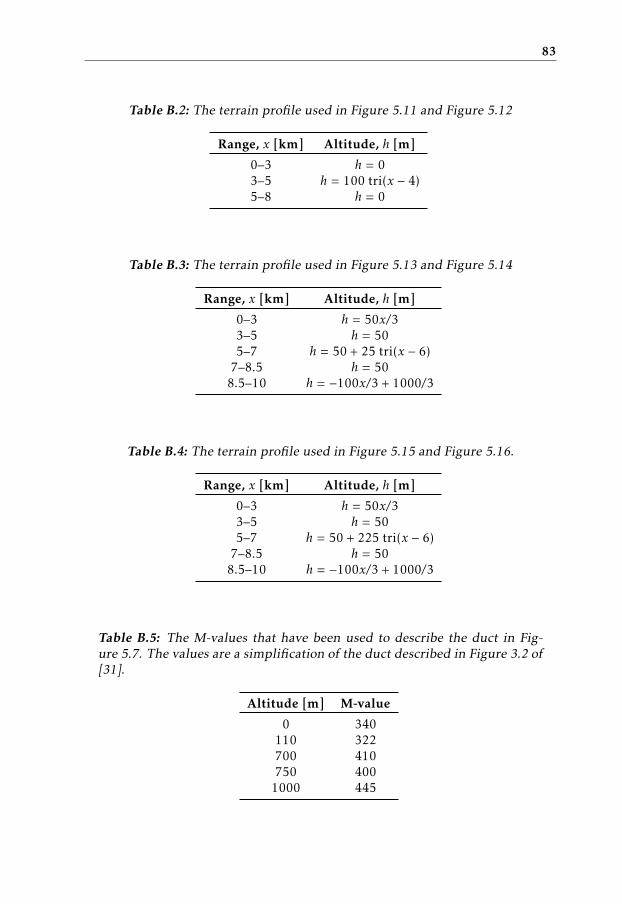
83

Table B.2: The terrain profile used in Figure 5.11 and Figure 5.12

Range, x [km] Altitude, h [m]

0–3 h = 03–5 h = 100 tri(x − 4)5–8 h = 0

Table B.3: The terrain profile used in Figure 5.13 and Figure 5.14

Range, x [km] Altitude, h [m]

0–3 h = 50x/33–5 h = 505–7 h = 50 + 25 tri(x − 6)7–8.5 h = 508.5–10 h = −100x/3 + 1000/3

Table B.4: The terrain profile used in Figure 5.15 and Figure 5.16.

Range, x [km] Altitude, h [m]

0–3 h = 50x/33–5 h = 505–7 h = 50 + 225 tri(x − 6)7–8.5 h = 508.5–10 h = −100x/3 + 1000/3

Table B.5: The M-values that have been used to describe the duct in Fig-ure 5.7. The values are a simplification of the duct described in Figure 3.2 of[31].

Altitude [m] M-value

0 340110 322700 410750 4001000 445

84 B Simulation parameters

Table B.6: M-values for an elevated duct measured at 04:00 October 8, 1949.As described by Burrows and Attwood [53].

Altitude [feet] M-value Altitude [feet] M-value

0 321 660 32960 322 720 330120 324 780 332180 327 840 334240 329 900 336300 331 960 340360 334 1020 342420 336 1080 344480 337 1140 346540 338 1200 349600 329

Bibliography

[1] J. C. Maxwell. A dynamical theory of the electromagnetic field. PhilosoficalTransactions of the Royal Society A, 155:459–512, 1865.

[2] D. E. Kerr. Propagation of Short Radio Waves. Number 13 inMassachusetts Institute of Technology Radiation Laboratory Series.McGraw-Hill Book Company, 1951.

[3] M. I. Skolnik. Introduction to Radar Systems. McGraw-Hill BookCompany, 2nd edition, 1980. ISBN 0-07-057909-1.

[4] H. R. Reed and C. M. Russell. Ultra High Frequency Propagation. JohnWiley Sons, Inc., 1953.

[5] A. E. Barrios. "Considerations in the development of the advancedpropagation model (APM) for U.S. navy applications", April 2005.

[6] Ö. Özgün, G. Apaydin, M. Kuzuoglu, and L. Sevgi. PETOOL:MATLAB-based one-way and two-way split-step parabolic equation toolfor radiowave propagation over variable terrain. Computer PhysicsCommunications, 182(12):2638–2654, December 2011. doi:10.1016/j.cpc.2011.07.017.

[7] World Meteorological Organization. "Manual on codes, internationalcodes, volume I.1, annex ii to the WMO technical regulations, part a -alphanumeric codes", 2018.

[8] M. Levy. Parabolic equation methods for electromagnetic wavepropagation. Electromagnetic wave series 45. The Institution of ElectricalEngineers, Stevenage, United Kingdom, 2000. ISBN 0-85296-764-0.

[9] D. K. Cheng. Field and Wave Electromagnetics. Pearson Education, Essex,England, 2nd edition, 2014. ISBN 978-1-292-02656-5.

[10] D. J. Griffiths. Introduction to Electrodynamics. Cambridge UniversityPress, Cambridge, 4th edition, 2017. ISBN 978-1-108-42041-9.

85

86 Bibliography

[11] P. Beckmann and A. Spizzichino. The Scattering of Electromagnetic Wavesfrom Rough Surfaces. Artech House, Inc., Norwood, MA., 1987. ISBN0-89006-238-2.

[12] M. Leontovich and V. Fock. Solution of the problem of propagation ofelectromagnetic waves along the Earth’s surface by the method of parabolicequation. Journal of Physics USSR, 10:13–24, 1946.

[13] R. H. Hardin and F. D. Tappert. Applications of the split-step Fouriermethod to the numerical solution of nonlinear and variable coefficientwave equations. SIAM Review, 15(2):423, 1973.

[14] P. Holm and G. Eriksson. "Parabolisk ekvationsteknik för vegetation",December 2002. FOI-R–0637–SE.

[15] F. J. Ryan. "Analysis of electromagnetic propagation over variable terrainusing the parabolic wave equation", October 1991. Technical Report 1453.

[16] G. Apaydin and L. Sevgi. The split-step-Fourier and finite-element-basedparabolic-equation propagation-prediction tools: Canonical tests,systematic comparisons and calibration. IEEE Antennas and PropagationMagazine, 52(3):66–79, June 2010. doi: 10.1109/MAP.2010.5586576.

[17] A. Barrios. A terrain parabolic equation model for propagation in thetroposphere. IEEE Transactions on Antennas and Propagation, 42(1):90–98, January 1994. doi: 10.1109/8.272306.

[18] J. R. Kuttler and G. D. Dockery. Theoretical description of the parabolicapproximation/Fourier split-step method of representing electromagneticpropagation in the troposphere. Radio Science, 26(2):381–393,March–April 1991. doi: 10.1029/91RS00109.

[19] G. P. Agrawal. Nonlinear Fiber Optics. Academic Press, Burlington, 4thedition, 2007. ISBN 978-0-12-369516-1.

[20] N. Hatano and M. Suzuki. Finding Exponential Product Formulas ofHigher Orders. Springer-Verlag, Berlin/Heidelberg, 2005. ISBN978-3-540-31515-5.

[21] M. D. Feit and J. A. Jr. Fleck. Light propagation in graded-index opticalfibers. Applied Optics, 17(24):3990–3998, December 1978. doi:10.1364/AO.17.003990.

[22] L. Råde and B. Westergren. Mathematics Handbook for Science andEngineering. Studentlitteratur, Lund, 4th edition, 1998. ISBN91-44-00839-2.

[23] S. Blanes, F. Casas, J. A. Oteo, and J. Ros. The Magnus expansion and someof its applications. Physics Reports, 470(5–6):151–283, January 2008. doi:10.1016/j.physrep.2008.11.001.

Bibliography 87

[24] P. D. Holm. Wide-angle shift-map PE for a piecewise linear terrain – afinite-difference approach. IEEE Transactions on Antennas andPropagation, 55(10):2773–2789, October 2007. doi:10.1109/TAP.2007.905865.

[25] M. F. Levy. Horizontal parabolic equation solution of radiowavepropagation problems on large domains. IEEE Transactions on Antennasand Propagation, 43(2):137–144, February 1995. doi: 10.1109/8.366375.

[26] G.A. Korn and T.M. Korn. Mathematical handbook for scientists andengineers: definitions, theorems, and formulas for reference and review.Dover Publications, Inc., Mineloa, New York, 2nd edition, 1968. ISBN978-0-486-41147-7.

[27] C. Nordling and J. Österman. Physics Handbook for Science andEngineering. Studentlitteratur, Lund, 8:13 edition, 2006. ISBN978-91-44-04453-8.

[28] B. R. Bean and E. J. Dutton. Radio Meteorology. National Bureau ofStandards, Washington D.C., 1966. National Bureau of StandardsMonograph 92.

[29] H. W. Ko, J. W. Sari, and J. P. Skura. Anomalous microwave propagationthrough atmospheric ducts. Johns Hopkins APL Technical Digest, 4(1):12–26, 1983.

[30] IEEE Antennas and Propagation Society. "IEEE standard definition ofterms for radio waves propagation", 2018.

[31] O. Gustafsson, G. Eriksson, P. Holm, A. Hågård, E. Karlsson,M. Nordstrand, R. Persson, P. von Schoenberg, and Å. Waern. "Slutrapportför projektet vågutbredningsanalys för radio, radar och elektrooptiskasystem", October 2003. FOI-R–0985–SE.

[32] SMHI. Nederbördsintensitet, October 2015. URL http://smhi.se/kunskapsbanken/meteorologi/nederbordsintensitet-1.19163.[Accessed: 2019-05-07].

[33] L. M. Brekhovskikh. Waves in Layered Media. Academic Press, New York,2nd edition, 1980. ISBN 0-12-130560-0.

[34] International Telecommunications Union. "Recommendation ITU-RP.527-4", 2017.

[35] G. D. Dockery and J. R. Kuttler. An improved impedance-boundaryalgorithm for Fourier split-step solutions of the parabolic wave equation.IEEE Transactions on Antennas and Propagation, 40(12):1592–1599,December 1996. doi: 10.1109/8.546245.

[36] G. D. Dockery. Modeling electromagnetic wave propagation in thetroposphere using the parabolic equation. IEEE Transactions on Antennasand Propagation, 36(10):1464–1470, October 1988. doi: 10.1109/8.8634.

88 Bibliography

[37] D. J. Donohue and J. R. Kuttler. Propagation modeling over terrain usingthe parabolic wave equation. IEEE Transactions on Antennas andPropagation, 48(2):260–277, February 2000. doi: 10.1109/8.833076.

[38] O. Benhmammouch, A. Khenchaf, and N. Caouren. Modelling roughnesseffects on propagation of electromagnetic waves in a maritimeenvironment: a hybrid approach. IET Radar, Sonar & Navigation, 5(9):1018–1025, December 2011. doi: 10.1049/iet-rsn.2009.0078.

[39] T. Elfouhaily, B. Chapron, K. Katsaros, and D. Vandemark. A unifieddirectional spectrum for long and short wind-driven waves. Journal ofGeophysical Research C: Oceans, 102(C7):15781–15796, July 1997. doi:10.1029/97JC00467.

[40] W. J. Pierson Jr and L. Moskowitz. "A proposed spectral form for fullydeveloped wind seas based on the similarity theory of S.A. Kitaigorodskii",October 1963.

[41] Q. Liu, F. Weng, and S. J. English. An improved fast microwave wateremissivity model. IEEE Transactions on Geoscience and Remote Sensing,49(4):1238–1250, April 2011. doi: 10.1109/TGRS.2010.2064779.

[42] A. R. Miller, R. M. Brown, and E. Vegh. New derivation for therough-surface reflection coefficient and for the distribution of sea-waveelevations. IEE Proceedings H - Microwaves, Optics and Antennas, 131(2):114–116, April 1984. doi: 10.1049/ip-h-1.1984.0022.

[43] I. Sirkova. Brief review on PE method application to propagation channelmodeling in sea environment. Central European Journal of Engineering, 2(1):19–38, March 2012. doi: 10.2478/s13531-011-0049-y.

[44] P. Zhang, L. Bai, Z. Wu, and L. Guo. Applying the parabolic equation totropospheric groundwave propagation. IEEE Antennas and PropagationMagazine, 58(3):31–44, June 2016. doi: 10.1109/MAP.2016.2541620.

[45] G. D. Dockery, R. S. Awadallah, D. E. Freund, J. Z. Gehman, and M. H.Newkirk. An overview of recent advances for the TEMPER radarpropagation model. In 2007 IEEE Radar Conference, pages 896–905,Boston, MA., U.S.A., April 2007. IEEE.

[46] D. J. Donohue and J. R. Kuttler. Modeling radar propagation over terrain.Johns Hopkins APL Technical Digest, 18(22):279–287, 1997.

[47] M. S. Lyatev. Nonlocal boundary conditions for split-step Padéapproximations of the Helmholtz equation with modified refractive index.IEEE Antennas and Wireless Propagation Letters, 17(8):13–24, August2018. doi: 10.1109/LAWP.2018.2855086.

[48] Computer Physics Communications Program Library. PETOOL (ParabolicEquation Toolbox), AEJS_v1_0, 2011. URL

Bibliography 89

http://cpc.cs.qub.ac.uk/summaries/AEJS_v1_0.html.[Accessed: 2019-04-05].

[49] Ö. Özgün. New software tool (GO+UTD) for visualization of wavepropagation [testing ourselves]. IEEE Antennas and Propagation, 58(3):91–103, June 2016. doi: 10.1109/MAP.2016.2541600.

[50] D. E. Freund, N. E. Woods, H-C. Ku, and R. S. Awadallah. Forward radarpropagation over a rough sea surface: A numerical assessment of theMiller-Brown approximation using a horizontally polarized 3-GHz linesource. IEEE Transactions on Antennas and Propagation, 54(4):1292–1304,April 2006. doi: 10.1109/TAP.2006.872669.

[51] B. W. Dowd and R. E. Díaz. FDTD simulation of very large domainsapplied to radar propagation over the ocean. IEEE Transactions onAntennas and Propagation, 66(10):5333–5348, October 2018. doi:10.1109/TAP.2018.2852141.

[52] Lantmäteriet. Höjddata, grid 50+, 2015. URL https://www.lantmateriet.se/sv/Kartor-och-geografisk-information/geodataprodukter/hojddata-grid-50/. [Accessed: 2019-04-19].

[53] C. R. Burrows and S. S. Attwood. Radio Wave Propagation. AcademicPress, New York, 1949.

[54] D.A. McNamara, C.W.I. Pistorius, and J.A.G. Malherbe. Introduction to thegeometrical theory of diffraction. Artech House, Norwood, MA, 1990.ISBN 0-89006-301-X.

[55] A. E. Barrios, W. L. Patterson, and R. A. Sprague. "Advanced propagationmodel (APM) version 2.1.04 computer software configuration item (CSCI)documents", February 2007.