Developing a realistic view on the availability of renewable resources

for the road transport sector in the Netherlands in 2050

Internship Project

Vasileios Nastoss0216488

Nederlandse Organisatie voor Toegepast Natuurwetenschappelijk Onderzoek(Netherlands Organization for Applied Scientific Research)

Department of Environmentally Sustainable Transport

MentorRichard Smokers (TNO, EST)

Delft, The Netherlands

March 1st, 2011 – June 30th, 2011

University of TwenteFaculty of Engineering Technology (CTW)

MSc Sustainable Energy Technology

SupervisorJoy Clancy (UT, CSTM)

Delft, June 2011

1

Summary

In this study several scenarios on the Netherland’s road transport sector evolution were developed with respect to the future transport demand, the vehicle fleet composition, the vehicle and energy production efficiency improvements, and the energy mix in order to obtain an environmentally sustainable model for transportation in 2050. The reduction target in road transport well-to-wheel CO2 emissions with reference to 1990 levels was set to 60%, as mentioned in the most recent White Paper on Transport of the European Commission.

The scenario for the transport demand in 2050 was estimated using the projections by the Welfare and Environment (WLO) study of 2006, and the most recent estimates of the Netherlands Environmental Assessment Agency (PBL). Subsequently, three scenarios on vehicle fleet composition were created implementing data from PBL for the first one, from a policy scenario of the “EU Transport GHG: Routes to 2050?” report for the second, and assuming a further decoupling from fossil fuel technologies for the third. Another three scenarios were plotted based on different assumptions on vehicle powertrain energy consumption, each one assuming further increases in efficiency, reaching to the lowest (according to thermodynamics) consumption in the third scenario. Finally, three scenarios were created as well for the fuel and electricity mix, with the last one presupposing a system based 100% on renewable resources.

This procedure produced 27 scenarios for which the well-to-wheel CO2 emissions were calculated and compared with the targets set for 2050. The scenarios were further analyzed with respect to energy and land requirements and implications, the demand-supply mismatch, and the system’s sustainability and security. The range of results for CO2 emissions was found between zero and about 20 million tons, for energy consumption between about 200PJ and 450PJ, and for land use from 14% to 128% of the Netherlands. The lowest values referred were found for the most efficient fleet composition and the lowest consumption rates. It is worth mentioning that the lowest value on land use is provided by the energy mix which uses the highest rate of fossil resources.

One of the goals of this report was to discover the limits to growth of the road transport sector in the Netherlands. The results presented hereafter strengthen the author’s opinion that technological improvement is a necessary but not sufficient condition to achieve sustainability; changes in mentality, lifestyle, patterns of consumption and production, and social structure are needed.

2

Table of Contents

Summary ..........................................................................................................................................1Table of Contents .............................................................................................................................2Acronym list .....................................................................................................................................3Introduction ......................................................................................................................................41. Current data on the Netherlands road transport and energy sectors.............................................6

1.1 Road transport ........................................................................................................................61.2 A comparison of modern vehicles..........................................................................................71.3 Electricity generation in 1990 and 2010 ................................................................................9

2. Building Scenarios and Methodology on Calculations ..............................................................112.1 Introduction ..........................................................................................................................112.2 Transport Demand................................................................................................................112.3 Fleet Composition ................................................................................................................142.4 Vehicle consumption rates ...................................................................................................152.5 Energy production ................................................................................................................17

2.5.1 Biofuels .........................................................................................................................172.5.2 Solar power ...................................................................................................................192.5.3 Wind power ...................................................................................................................20

2.6 Electricity generation mix and fuel blend ............................................................................212.6 Emission Factors ..................................................................................................................222.7 Electricity mismatch and storage models.............................................................................242.8 A comparison of powertrain technologies ...........................................................................26

3. Calculations................................................................................................................................283.1 Energy consumption.............................................................................................................283.2 Land use ...............................................................................................................................313.3 Example of electricity mismatch and storage ......................................................................32

3.3.1 Day-time recharging......................................................................................................333.3.2 Night-time recharging ...................................................................................................33

3.4 The “electrifying” scenario ..................................................................................................344. Conclusions ................................................................................................................................36References ......................................................................................................................................38Appendix ........................................................................................................................................41Appendix ........................................................................................................................................41

3

Acronym list

a-Si Amorphous SiliconBEV Battery Electric VehiclesCADC Common Artemis Driving CycleCCS Carbon Capture and StorageCCGT Combined Cycle Gas Turbine CdTe Cadmium TellurideCIS Copper Indium DiselinideCNG Compressed Natural GasEC European CommissionECN Energy Research Centre of the NetherlandsEF Emission FactorEU European UnionEV Electric VehiclesFAO Food and Agriculture Organisation of the United NationsFCEV Fuel Cell Electric VehiclesFT Fischer-TropschGE Global EconomyGHG Greenhouse Gas(es)HDV Heavy Duty VehiclesHHV Higher Heating ValueICE Internal Combustion EngineIEA International Energy AgencyIEEP Institute for European Environmental PolicyILUC Indirect Land Use ChangeLAT Laboratory of Applied ThermodynamicsLi-ion Lithium ionLPG Liquid Petroleum Gasmc-Si Mono-crystalline SiliconMDV Medium Duty VehiclesNYBC New York Bus CyclePBL Netherlands Environmental Assessment AgencyPV Photovoltaicr-Si Ribbon Siliconsc-Si Single-crystal SiliconSTC Standard Test ConditionsTNO Netherlands Organization for Applied Scientific ResearchTTW Tank-To-WheelWHVC World Harmonized Vehicle CycleWLO Welfare and EnvironmentWTT Well-To-TankWTW Well-To-Wheel

4

Introduction

The European Union has expressed the ambition (as stated in Presidency Conclusions of the European Council, October 29/30 2009) that in 2050 industrialized countries must have reduced their CO2 emissions by at least 80% relative to the 1990 levels to keep global warming below the 2°C threshold. In order to contribute to this goal the European transport sector will have to reduce its CO2 emissions by 60% with respect to the 1990 corresponding emissions, provided that in other sectors larger reductions can be found.

One way to achieve this target could be the majority of vehicles in the fleet by 2050 to have becomemuch more efficient than current vehicles and run on sustainably produced, renewable energy. This renewable energy may be transferred to the vehicles in the form of e.g. biofuels, electricity, or hydrogen. Greenhouse gas reductions at the vehicle level will have to be augmented by efficiency improvements in the structure of the transport system and by management of the growth of transport volumes.

The feasibility of such a transition towards a sustainable mobility system in the 2010-2050 timeframe strongly depends on the availability of sufficient amounts of renewable energy. This renewable energy is not only necessary for the transport sector but also for all other sectors of the economy. The amount of renewable energy needed to "fuel" a sustainable mobility system depends on (growth in) the total transport performance, on the overall targets set for reduction of CO2 emissions and reduction of fossil fuel use, on vehicle tank-to-wheel efficiency and energy efficiency in the well-to-tank energy chain. The efficiencies are obviously limited by the laws of thermodynamics.

The required amount of renewable energy can be translated into land-use implications which depend on the energy yield per hectare that can be obtained for e.g. biomass production or centralized solar or wind energy production and e.g. on the level to which renewable energy production can be integrated into existing infrastructure (e.g. solar panels on buildings, conversion of agricultural crops and pasture fieldsfor biofuel production etc.). Besides land use impacts, the production of renewable energy may have other implications that limit its potential availability, e.g. the possible mismatch in time and place between renewable energy supply and transport energy demand.

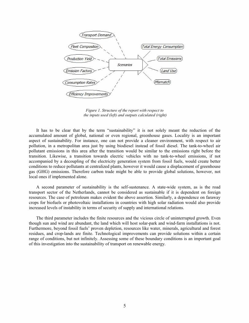
In this report several of these aspects are examined through possible future scenarios regarding the transition of the road transport sector towards sustainability. The structure of the report is schematically presented in Figure 1. Data and projections for the transport demand, the fleet composition, the production yields of several resources, the emission factors of fuels, the consumption rates of vehicles and the efficiency improvements are combined in order to create future scenarios which will provide the total energy consumption, the total emissions, the land use and the daily mismatch between demand and supply for the road transport sector of the Netherlands in 2050.

The scenarios are aiming to answer the following core questions: a) under which conditions can the road transport of the Netherlands meet the European Commission targets for carbon emission reductions; b) what the energy requirements will then be; c) how much land of renewable resources will be needed; and d) are these scenarios propelling sustainability?

5

Figure 1. Structure of the report with respect to the inputs used (left) and outputs calculated (right)

It has to be clear that by the term “sustainability” it is not solely meant the reduction of theaccumulated amount of global, national or even regional, greenhouse gases. Locality is an important aspect of sustainability. For instance, one can not provide a cleaner environment, with respect to air pollution, in a metropolitan area just by using biodiesel instead of fossil diesel. The tank-to-wheel air pollutant emissions in this area after the transition would be similar to the emissions right before the transition. Likewise, a transition towards electric vehicles with no tank-to-wheel emissions, if not accompanied by a decoupling of the electricity generation system from fossil fuels, would create better conditions to reduce pollutants at centralized plants, however it would cause a displacement of greenhouse gas (GHG) emissions. Therefore carbon trade might be able to provide global solutions, however, not local ones if implemented alone.

A second parameter of sustainability is the self-sustenance. A state-wide system, as is the road transport sector of the Netherlands, cannot be considered as sustainable if it is dependent on foreign resources. The case of petroleum makes evident the above assertion. Similarly, a dependence on faraway crops for biofuels or photovoltaic installations in countries with high solar radiation would also provide increased levels of instability in terms of security of supply and international relations.

The third parameter includes the finite resources and the vicious circle of uninterrupted growth. Even though sun and wind are abundant, the land which will host solar-park and wind-farm installations is not. Furthermore, beyond fossil fuels’ proven depletion, resources like water, minerals, agricultural and forest residues, and crop-lands are finite. Technological improvements can provide solutions within a certain range of conditions, but not infinitely. Assessing some of these boundary conditions is an important goal of this investigation into the sustainability of transport on renewable energy.

6

1. Current data on the Netherlands road transport and energy sectors

The first chapter provides an analysis on the present situation, in order to create a starting point for realistic projections for the future. This analysis is focused on road transport sector data, the energy production system, and vehicle development data.

1.1 Road transport

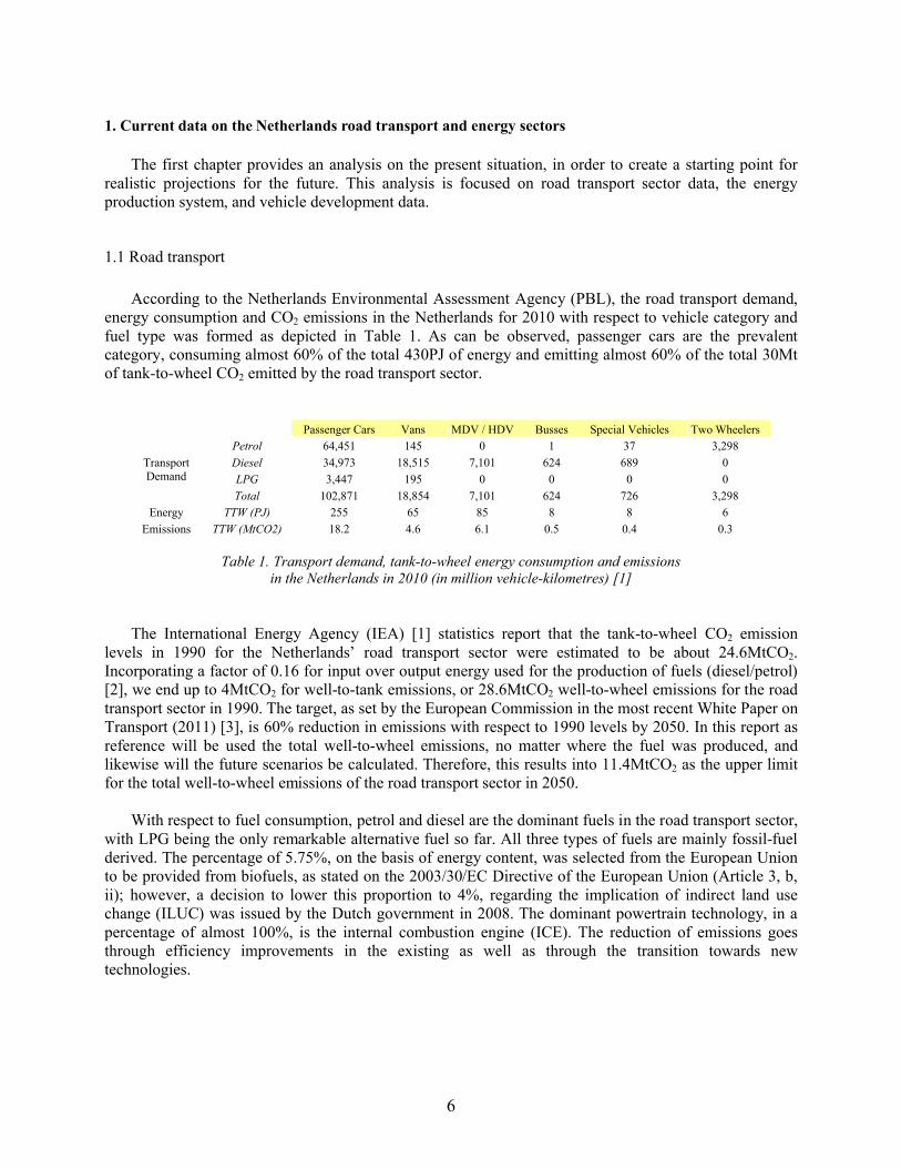
According to the Netherlands Environmental Assessment Agency (PBL), the road transport demand,energy consumption and CO2 emissions in the Netherlands for 2010 with respect to vehicle category and fuel type was formed as depicted in Table 1. As can be observed, passenger cars are the prevalent category, consuming almost 60% of the total 430PJ of energy and emitting almost 60% of the total 30Mt of tank-to-wheel CO2 emitted by the road transport sector.

Passenger Cars Vans MDV / HDV Busses Special Vehicles Two Wheelers

Petrol 64,451 145 0 1 37 3,298

Diesel 34,973 18,515 7,101 624 689 0

LPG 3,447 195 0 0 0 0

Transport Demand

Total 102,871 18,854 7,101 624 726 3,298

Energy TTW (PJ) 255 65 85 8 8 6

Emissions TTW (MtCO2) 18.2 4.6 6.1 0.5 0.4 0.3

Table 1. Transport demand, tank-to-wheel energy consumption and emissionsin the Netherlands in 2010 (in million vehicle-kilometres) [1]

The International Energy Agency (IEA) [1] statistics report that the tank-to-wheel CO2 emission levels in 1990 for the Netherlands’ road transport sector were estimated to be about 24.6MtCO2. Incorporating a factor of 0.16 for input over output energy used for the production of fuels (diesel/petrol)[2], we end up to 4MtCO2 for well-to-tank emissions, or 28.6MtCO2 well-to-wheel emissions for the road transport sector in 1990. The target, as set by the European Commission in the most recent White Paper on Transport (2011) [3], is 60% reduction in emissions with respect to 1990 levels by 2050. In this report as reference will be used the total well-to-wheel emissions, no matter where the fuel was produced, and likewise will the future scenarios be calculated. Therefore, this results into 11.4MtCO2 as the upper limit for the total well-to-wheel emissions of the road transport sector in 2050.

With respect to fuel consumption, petrol and diesel are the dominant fuels in the road transport sector, with LPG being the only remarkable alternative fuel so far. All three types of fuels are mainly fossil-fuel derived. The percentage of 5.75%, on the basis of energy content, was selected from the European Union to be provided from biofuels, as stated on the 2003/30/EC Directive of the European Union (Article 3, b, ii); however, a decision to lower this proportion to 4%, regarding the implication of indirect land use change (ILUC) was issued by the Dutch government in 2008. The dominant powertrain technology, in a percentage of almost 100%, is the internal combustion engine (ICE). The reduction of emissions goes through efficiency improvements in the existing as well as through the transition towards new technologies.

7

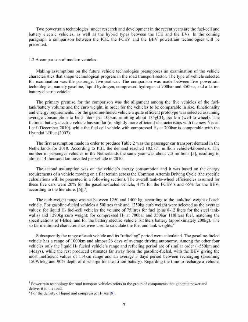
Two powertrain technologies1 under research and development in the recent years are the fuel-cell and battery electric vehicles, as well as the hybrid types between the ICE and the EVs. In the coming paragraph a comparison between the ICE, the FCEV and the BEV powertrain technologies will be presented.

1.2 A comparison of modern vehicles

Making assumptions on the future vehicle technologies presupposes an examination of the vehicle characteristics that shape technological progress in the road transport sector. The type of vehicle selected for examination was the passenger five-seat car. The comparison was made between five powertrain technologies, namely gasoline, liquid hydrogen, compressed hydrogen at 700bar and 350bar, and a Li-ion battery electric vehicle.

The primary premise for the comparison was the alignment among the five vehicles of the fuel-tank/battery volume and the curb weight, in order for the vehicles to be comparable in size, functionality and energy requirements. For the gasoline-fueled vehicle a quite efficient prototype was selected assuming average consumption to be 5 liters per 100km, emitting about 135gCO2 per km (well-to-wheel). The fictional battery electric vehicle has similar (or slightly more efficient) characteristics with the new Nissan Leaf (December 2010), while the fuel cell vehicle with compressed H2 at 700bar is comparable with the Hyundai I-Blue (2007).

The first assumption made in order to produce Table 2 was the passenger car transport demand in the Netherlands for 2010. According to PBL the demand reached 102,871 million vehicle-kilometers. Thenumber of passenger vehicles in the Netherlands the same year was about 7.3 millions [5], resulting to almost 14 thousand km travelled per vehicle in 2010.

The second assumption was on the vehicle’s energy consumption and it was based on the energy requirements of a vehicle moving on a flat terrain across the Common Artemis Driving Cycle (the specific calculations will be presented in a following section). The overall tank-to-wheel efficiencies assumed for these five cars were 20% for the gasoline-fueled vehicle, 41% for the FCEV’s and 65% for the BEV, according to the literature. [6][7]

The curb-weight range was set between 1250 and 1400 kg, according to the tank/fuel weight of each vehicle. For gasoline-fueled vehicles a 50litres tank and 1250kg curb weight were selected as the averagevalues; for liquid H2 fuel-cell vehicles the volume of 75litres for fuel (plus 8-12 liters for the steel tank-walls) and 1290kg curb weight; for compressed H2 at 700bar and 350bar 110liters fuel, matching the specifications of I-Blue; and for the battery electric vehicle 165liters battery (approximately 200kg). The so far mentioned characteristics were used to calculate the fuel and tank weights.2

Subsequently the range of each vehicle and its “refueling” period were calculated. The gasoline-fueled vehicle has a range of 1000km and almost 26 days of average driving autonomy. Among the other four vehicles only the liquid H2 fueled vehicle’s range and refueling period are of similar order (~550km and 14days), while the rest produced estimates far away from the gasoline-fueled, with the BEV giving the most inefficient values of 114km range and an average 3 days period between recharging (assuming 150Wh/kg and 90% depth of discharge for the Li-ion battery). Regarding the time to recharge a vehicle,

1 Powertrain technology for road transport vehicles refers to the group of components that generate power and deliver it to the road.2 For the density of liquid and compressed H2 see [8].

8

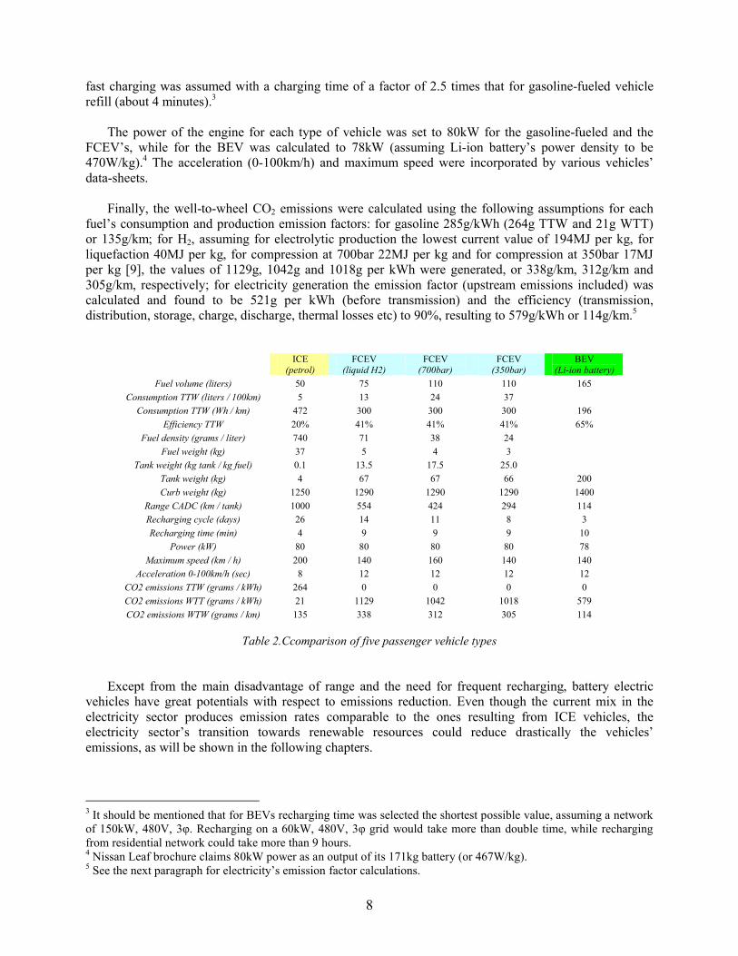
fast charging was assumed with a charging time of a factor of 2.5 times that for gasoline-fueled vehicle refill (about 4 minutes).3

The power of the engine for each type of vehicle was set to 80kW for the gasoline-fueled and the FCEV’s, while for the BEV was calculated to 78kW (assuming Li-ion battery’s power density to be 470W/kg).4 The acceleration (0-100km/h) and maximum speed were incorporated by various vehicles’ data-sheets.

Finally, the well-to-wheel CO2 emissions were calculated using the following assumptions for each fuel’s consumption and production emission factors: for gasoline 285g/kWh (264g TTW and 21g WTT) or 135g/km; for H2, assuming for electrolytic production the lowest current value of 194MJ per kg, for liquefaction 40MJ per kg, for compression at 700bar 22MJ per kg and for compression at 350bar 17MJ per kg [9], the values of 1129g, 1042g and 1018g per kWh were generated, or 338g/km, 312g/km and 305g/km, respectively; for electricity generation the emission factor (upstream emissions included) was calculated and found to be 521g per kWh (before transmission) and the efficiency (transmission, distribution, storage, charge, discharge, thermal losses etc) to 90%, resulting to 579g/kWh or 114g/km.5

ICE(petrol)

FCEV (liquid H2)

FCEV (700bar)

FCEV (350bar)

BEV(Li-ion battery)

Fuel volume (liters) 50 75 110 110 165

Consumption TTW (liters / 100km) 5 13 24 37

Consumption TTW (Wh / km) 472 300 300 300 196

Efficiency TTW 20% 41% 41% 41% 65%

Fuel density (grams / liter) 740 71 38 24

Fuel weight (kg) 37 5 4 3

Tank weight (kg tank / kg fuel) 0.1 13.5 17.5 25.0

Tank weight (kg) 4 67 67 66 200

Curb weight (kg) 1250 1290 1290 1290 1400

Range CADC (km / tank) 1000 554 424 294 114

Recharging cycle (days) 26 14 11 8 3

Recharging time (min) 4 9 9 9 10

Power (kW) 80 80 80 80 78

Maximum speed (km / h) 200 140 160 140 140

Acceleration 0-100km/h (sec) 8 12 12 12 12

CO2 emissions TTW (grams / kWh) 264 0 0 0 0

CO2 emissions WTT (grams / kWh) 21 1129 1042 1018 579

CO2 emissions WTW (grams / km) 135 338 312 305 114

Table 2.Ccomparison of five passenger vehicle types

Except from the main disadvantage of range and the need for frequent recharging, battery electric vehicles have great potentials with respect to emissions reduction. Even though the current mix in the electricity sector produces emission rates comparable to the ones resulting from ICE vehicles, the electricity sector’s transition towards renewable resources could reduce drastically the vehicles’ emissions, as will be shown in the following chapters.

3 It should be mentioned that for BEVs recharging time was selected the shortest possible value, assuming a network of 150kW, 480V, 3φ. Recharging on a 60kW, 480V, 3φ grid would take more than double time, while recharging from residential network could take more than 9 hours. 4 Nissan Leaf brochure claims 80kW power as an output of its 171kg battery (or 467W/kg).5 See the next paragraph for electricity’s emission factor calculations.

9

Furthermore, in terms of tank-to-wheel energy consumption, a battery electric vehicle is almost 60% more efficient, than an ICE vehicle. Projecting these vehicles in the future, regarding a system based mainly on renewable resources, the differences range from a factor of 3 to a factor of 20, between electric and fuel-based vehicles. The calculations were made with respect to land use and are analyzed in Chapter II.

As most important factors, according to current trends and lifestyle and future environmental needs, on which technological progress on electric vehicles should focus are suggested the two following: decarbonisation of electricity production and improved vehicle autonomy (or range and “refueling” period). The improvements so far, especially with respect to the autonomy, are regarded as insufficient primarily for long-distance transport of goods and people, making the decoupling from fossil fuel technologies in categories like duty vehicles and coaches improbable for the short term future. Furthermore, as long as electricity generation is largely dependent on fossil fuels, the well-to-wheel emissions of the transport sector will remain high even if the transport fleet is turned to fuel-cell and battery electric vehicles, technologies which have zero tank-to-wheel emissions.

1.3 Electricity generation in 1990 and 2010

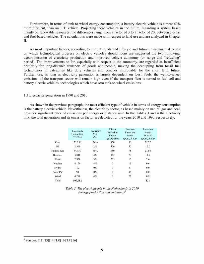
As shown in the previous paragraph, the most efficient type of vehicle in terms of energy consumption is the battery electric vehicle. Nevertheless, the electricity sector, as based mainly on natural gas and coal, provides significant rates of emissions per energy or distance unit. In the Tables 3 and 4 the electricity mix, the total generation and its emission factor are depicted for the years 2010 and 1990, respectively.

Electricity Generation(GWh/a)

Electricity Mix(%)

Direct Emission

Factor (gCO2/kWh)

Upstream Emission

Factor (gCO2/kWh)

Emission FactorIn Mix

(gCO2/kWh)Coal 25,250 24% 850 50 212.2

Oil 2,340 2% 500 50 12.0

Natural Gas 64,150 60% 380 75 272.6

Biomass 3,810 4% 342 70 14.7

Waste 2,920 3% 265 15 7.6

Nuclear 4,170 4% 0 15 0.6

Hydro 102 0% 0 8 0.0

Solar PV 50 0% 0 86 0.0

Wind 4,290 4% 0 23 0.9

Total 107,082 521

Table 3. The electricity mix in the Netherlands in 2010 (energy production and emissions)6

6 Sources: [12][13][14][15][16][15][16]

10

Electricity Generation

(TWh/a)

Electricity Mix(%)

Direct Emission

Factor (gCO2/kWh)

Upstream Emission

Factor (gCO2/kWh)

Emission FactorIn Mix

(gCO2/kWh)Coal 25 34% 1,159 60 412

Oil 3 4% 274 60 14

Natural Gas 40 54% 400 80 259

Nuclear 4 5% 0 20 1

Renewables 2 3% 0 40 2

Total 74 688

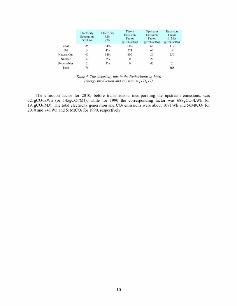
Table 4. The electricity mix in the Netherlands in 1990 (energy production and emissions) [17][17]

The emission factor for 2010, before transmission, incorporating the upstream emissions, was 521gCO2/kWh (or 145gCO2/MJ), while for 1990 the corresponding factor was 688gCO2/kWh (or 191gCO2/MJ). The total electricity generation and CO2 emissions were about 107TWh and 56MtCO2 for 2010 and 74TWh and 51MtCO2 for 1990, respectively.

11

2. Building Scenarios and Methodology on Calculations

2.1 Introduction

In this chapter the steps followed to make projections and build the future scenarios for the road transport sector in the Netherlands are presented. Several scientific reports were reviewed in order to create realistic assumptions and set the basis for the calculations in the third chapter.

The future scenarios incorporate data regarding the transport demand, the fleet composition, the production yields of several energy generation technologies placed in the Netherlands, the emission factors of each vehicle and energy production technology, the consumption rate of each vehicle and the assumptions on efficiency improvements with respect to tank-to-wheel consumption and well-to-tank production and losses.

The results on total energy consumption and emissions, as well as the calculations on land use, land use implications and daily supply-demand mismatch will be presented in the third chapter.

2.2 Transport Demand

The first step of this study in order to realize the future scenarios was the definition of the total road transport volume in 2050 per vehicle category (depending on mass and mode, i.e. passenger cars, vans, freight vehicles, busses, special vehicles and two-wheelers). The transport demand scenario of this case study was created incorporating data from two reports, namely the study Welfare and Environment (WLO) of 2006 [18], and the most recent estimations of PBL [19], regarding the Dutch road transport sector.

From the WLO report the Global Economy scenario (“GE2006” hereafter) was selected as the most realistic trend (business as usual) for transport growth compared to the other three scenarios developed in the same study. As the estimations of the referred report reached until 2040, its projected data were extrapolated to 2050. The more recent PBL forecasts, namely scenario RR2010, incorporated more accurate data for the years 2000 and 2005, and took into account the economic recession of the recent years in order to create projections for 2030. For the present study the data were extrapolated to 2050 and compared with the GE2006 scenario.

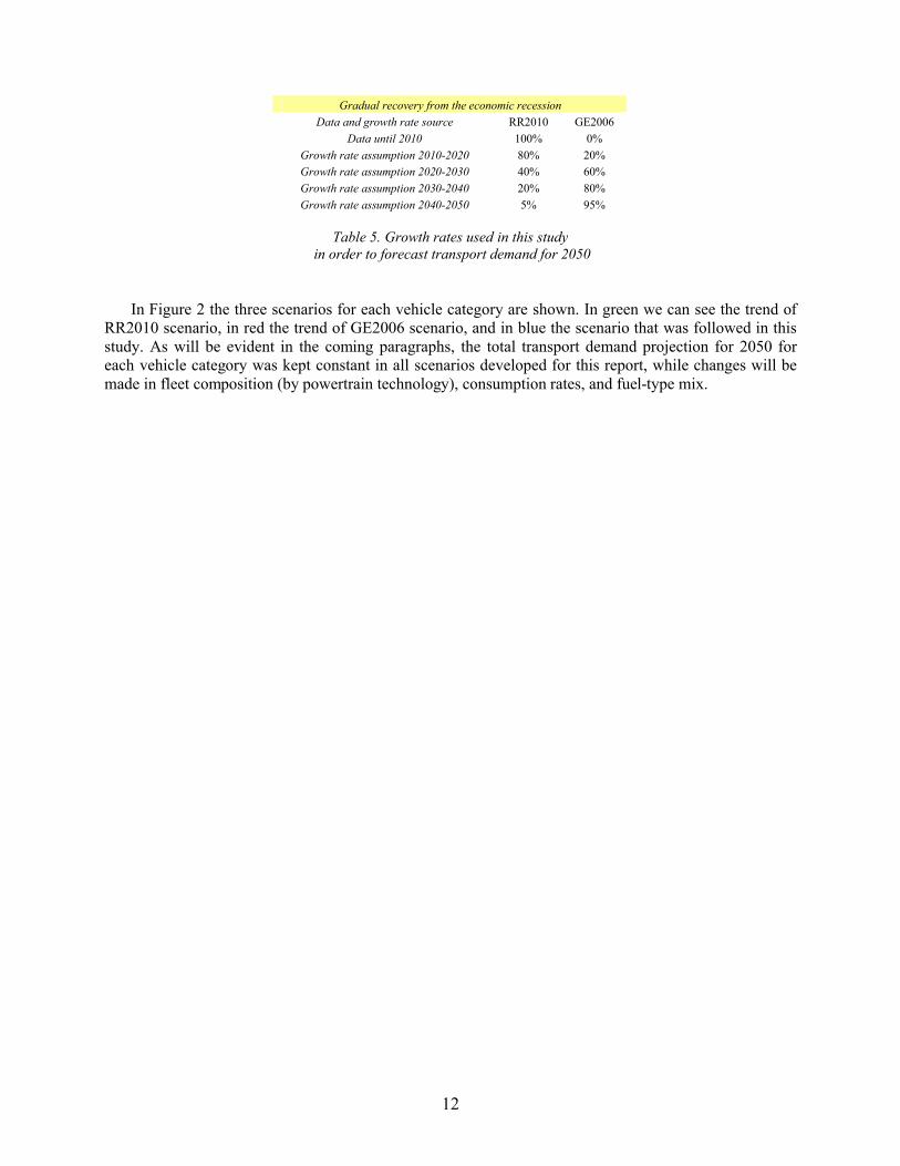
The scenario for road transport demand in the Netherlands for 2050 was based on the assumptions shown in Table 5. Until 2010 the data provided from RR2010, which were regarded as more accurate, were incorporated unaltered. Then the period until 2050 was divided into four 10-year segments and the transport growth rate for each scenario (GE2006 and RR2010) in each segment was calculated. A weighing factor was applied in the growth rates of each scenario, starting from 80% for RR2010 rate for the period 2010-2020 and decreasing its influence by 50% from segment to segment. The influence reduction of the RR2010 scenario was based on the assumption that the growth rates will gradually return to a more Global-Economy-like trends through a steady recovery from the economic recession, following a business-as-usual trend.

12

Gradual recovery from the economic recession

Data and growth rate source RR2010 GE2006

Data until 2010 100% 0%

Growth rate assumption 2010-2020 80% 20%

Growth rate assumption 2020-2030 40% 60%

Growth rate assumption 2030-2040 20% 80%

Growth rate assumption 2040-2050 5% 95%

Table 5. Growth rates used in this study in order to forecast transport demand for 2050

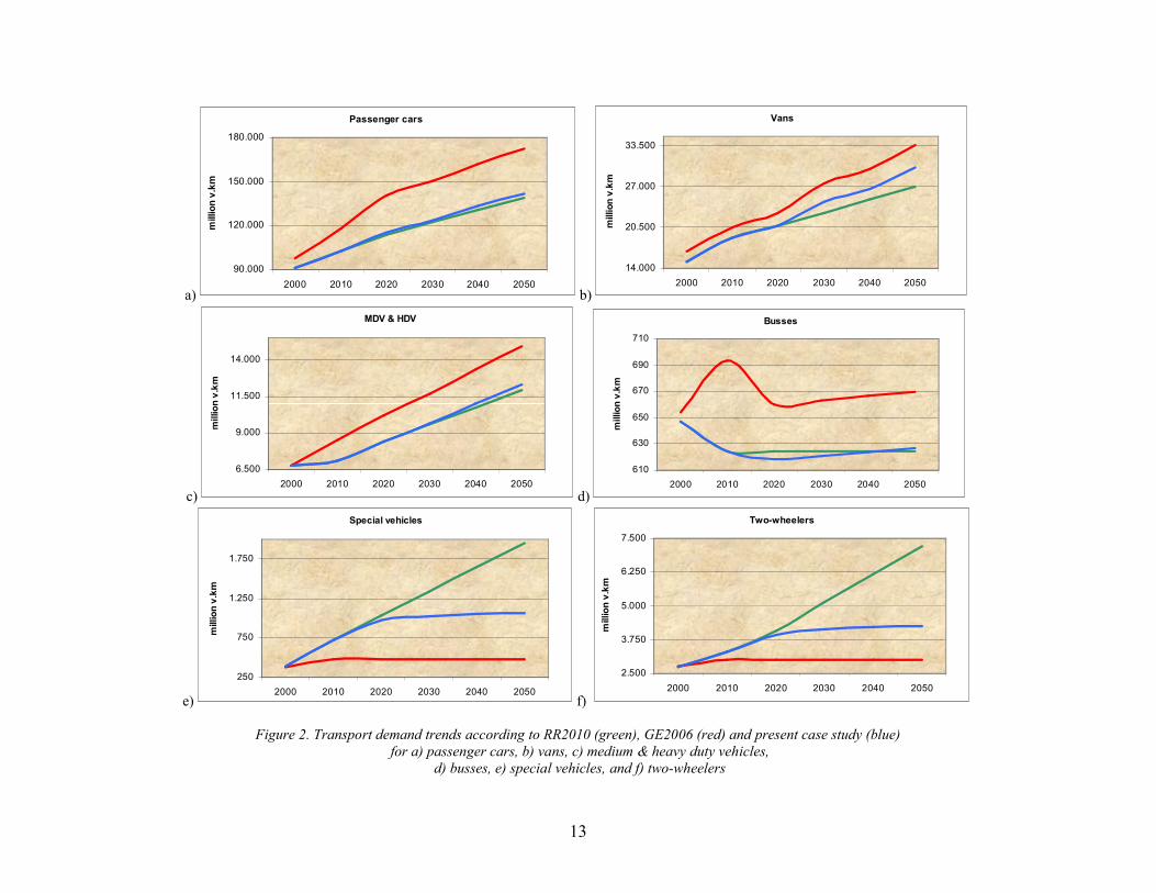
In Figure 2 the three scenarios for each vehicle category are shown. In green we can see the trend of RR2010 scenario, in red the trend of GE2006 scenario, and in blue the scenario that was followed in this study. As will be evident in the coming paragraphs, the total transport demand projection for 2050 for each vehicle category was kept constant in all scenarios developed for this report, while changes will be made in fleet composition (by powertrain technology), consumption rates, and fuel-type mix.

13

a)

Passenger cars

90.000

120.000

150.000

180.000

2000 2010 2020 2030 2040 2050

mill

ion

v.k

m

b)

Vans

14.000

20.500

27.000

33.500

2000 2010 2020 2030 2040 2050

mill

ion

v.k

m

c)

MDV & HDV

6.500

9.000

11.500

14.000

2000 2010 2020 2030 2040 2050

mill

ion

v.k

m

d)

Busses

610

630

650

670

690

710

2000 2010 2020 2030 2040 2050

mill

ion

v.k

m

e)

Special vehicles

250

750

1.250

1.750

2000 2010 2020 2030 2040 2050

mill

ion

v.k

m

f)

Two-wheelers

2.500

3.750

5.000

6.250

7.500

2000 2010 2020 2030 2040 2050

mill

ion

v.k

m

Figure 2. Transport demand trends according to RR2010 (green), GE2006 (red) and present case study (blue) for a) passenger cars, b) vans, c) medium & heavy duty vehicles,

d) busses, e) special vehicles, and f) two-wheelers

14

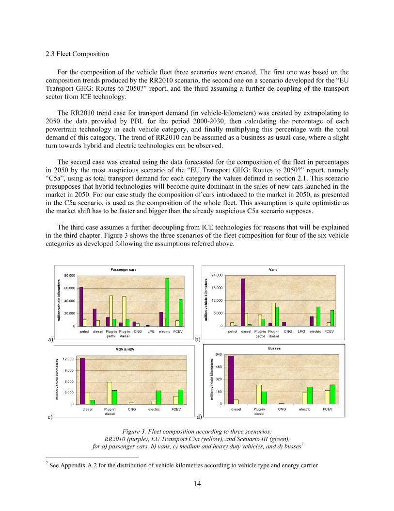
2.3 Fleet Composition

For the composition of the vehicle fleet three scenarios were created. The first one was based on the composition trends produced by the RR2010 scenario, the second one on a scenario developed for the “EU Transport GHG: Routes to 2050?” report, and the third assuming a further de-coupling of the transport sector from ICE technology.

The RR2010 trend case for transport demand (in vehicle-kilometers) was created by extrapolating to 2050 the data provided by PBL for the period 2000-2030, then calculating the percentage of each powertrain technology in each vehicle category, and finally multiplying this percentage with the total demand of this category. The trend of RR2010 can be assumed as a business-as-usual case, where a slight turn towards hybrid and electric technologies can be observed.

The second case was created using the data forecasted for the composition of the fleet in percentages in 2050 by the most auspicious scenario of the “EU Transport GHG: Routes to 2050?” report, namely “C5a”, using as total transport demand for each category the values defined in section 2.1. This scenario presupposes that hybrid technologies will become quite dominant in the sales of new cars launched in the market in 2050. For our case study the composition of cars introduced to the market in 2050, as presented in the C5a scenario, is used as the composition of the whole fleet. This assumption is quite optimistic as the market shift has to be faster and bigger than the already auspicious C5a scenario supposes.

The third case assumes a further decoupling from ICE technologies for reasons that will be explained in the third chapter. Figure 3 shows the three scenarios of the fleet composition for four of the six vehicle categories as developed following the assumptions referred above.

a)

Passenger cars

0

20.000

40.000

60.000

80.000

petrol diesel Plug-inpetrol

Plug-indiesel

CNG LPG electric FCEV

mill

ion

ve

hic

le k

ilom

ete

rs

b)

Vans

0

6.000

12.000

18.000

24.000

petrol diesel Plug-inpetrol

Plug-indiesel

CNG LPG electric FCEV

mill

ion

ve

hic

le k

ilom

ete

rs

c)

MDV & HDV

0

3.000

6.000

9.000

12.000

diesel Plug-indiesel

CNG electric FCEV

mill

ion

ve

hic

le k

ilom

ete

rs

d)

Busses

0

160

320

480

640

diesel Plug-indiesel

CNG electric FCEV

mill

ion

veh

icle

kilo

me

ters

Figure 3. Fleet composition according to three scenarios: RR2010 (purple), EU Transport C5a (yellow), and Scenario III (green),

for a) passenger cars, b) vans, c) medium and heavy duty vehicles, and d) busses7

7 See Appendix A.2 for the distribution of vehicle kilometres according to vehicle type and energy carrier

15

In the RR2010 scenario (purple in Figure 3) the dependence on petrol, diesel and their substitutes is really high in passenger cars and vans (more than 70%, taking into account the hybrid vehicles as well), while in medium and heavy duty vehicles and busses diesel and its substitutes consist 100% of the fuel used. The C5a scenario (yellow in Figure 3) relies more on hybrid technology, assuming penetrations of 70% in passenger cars, about 50% in light, medium and heavy duty vehicles, and almost 40% in busses. The third scenario (green in Figure 3) depends more on the electric vehicles (battery and fuel-cell) and minimizes the ICE technologies. This scenario is very optimistic and presupposes advanced technological improvements and market shifts.

2.4 Vehicle consumption rates

In order to calculate the consumption of the vehicles examined in this study, three scenarios were created. In the first scenario (moderate) the consumption of all vehicles was reduced by 10% with reference to the consumption calculated by the estimations on vehicle-kilometers and total energy consumption in the RR2010 study for the year 2030. In the second scenario (average) the consumption of all vehicles was further reduced with reference to the first scenario, and calculated as the average consumption between the moderate scenario (first) and the limits scenario (third).

The third scenario (limits) calculates the minimum energy required for a vehicle to drive an official driving cycle of its category on a flat terrain. It provides calculations on the energy required to accelerate Eacc (equation 4), to compensate the rolling resistance Err (equation 5) and to overcome the drag force Edrag

(equation 6).

Symbol Definition Unit Symbol Definition Unitm Curb weight kg D Distance travelled mv Velocity m/s cd Drag coefficient -α Acceleration m/s2 A Frontal area m2

g Gravitational acceleration m/s2 ρ Air density kg/m3

crr Rolling resistance coefficient - t Time elapsed sec

Table 6. Definitions and units for the symbols in equations (1) – (6)

The values picked for air density and gravitational acceleration were 1.2kg/m3 and 9.81m/s2, respectively. For curb weight, rolling resistance coefficient, drag coefficient, and frontal area the values selected for each vehicle category are shown in Table 7.

16

Passenger cars Vans MDV HDV Busses

Class Class 1 Class 2 Class 3, 4, 5 Class 6, 7, 8 Base Classe

Reference year 2010 2050 2010 2050 2010 2050 2010 2050 2010 2050

Average curb and load weight (kg) 1250 1000 2700 2500 7000 6800 14500 14300 12900 12500

Drag coefficient 0.34 0.17 0.42 0.30 0.51 0.47 0.56 0.51 0.70 0.65

Frontal area (m2) 2.4 1.9 3.0 2.1 4.5 3.3 9.7 6.9 7.5 7.2

Rolling resistance coefficient 0.0080 0.0070 0.0070 0.0065 0.0065 0.0060 0.0051 0.0049 0.0056 0.0051

Table 7. Vehicle characteristics according to vehicle category

The driving cycles that were used for the optimum case were: for passenger cars and vans the Common Artemis Driving Cycle UM130 (CADC); for medium and heavy duty vehicles the World Harmonized Vehicle Cycle (WHVC); and for busses the New York Bus Cycle (NYBC). The results which occurred from this process are depicted in Table 8. The values refer to the energy consumed at the wheels due to acceleration, rolling resistance, and drag force, with respect to the characteristics of vehicles (as referred in Table 7) and the specifications of the driving cycles (as mentioned in Appendix A.1).

Passenger cars(CADC)

Vans(CADC)

MDV(WHVC)

HDV(WHVC)

Busses(NYBC)

MJ/km 0.34 0.78 1.29 2.43 4.17

kWh/km 0.095 0.216 0.358 0.675 1.159

Table 8. Energy consumption at the wheels for each vehicle category in a specific driving cycle

In Table 9 the tank-to-wheel efficiencies assumed for battery electric, internal combustion engine and fuel-cell electric vehicles for the optimum case study of the projections for 2050 are presented in comparison with the corresponding present values. For ICE and FCEV an increase of about 15% in tank-to-wheel efficiency was assumed, while for battery electric vehicles the corresponding value was set to 25%.

2010 2050 2010 2050Battery Electric Internal Combustion Engine

Inverter / motor efficiency 87% 96% TTW fuel efficiency 26% 26%

Gear box efficiency 92% 97% Total (incorporating engine losses) 20% 23%

Charge / discharge efficiency 85% 96% Fuel-Cell Electric

DC rectifier efficiency 96% 98% TTW fuel efficiency 50% 53%

Total 65% 88% Total (incorporating engine losses) 41% 46%

Table 9. Vehicle tank-to-wheel efficiencies as collected from literature for 2010 and selected for the optimum case for 2050

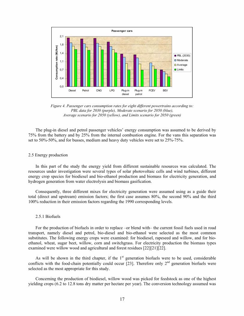
In Figure 4 the example of passenger cars was selected to illustrate the efficiency improvements for 2050 in the three scenarios mentioned above. A comparison is as well made with the projected data for 2030 as found in the PBL study (purple in Figure 4).

17

Passenger cars

0,0

0,4

0,7

1,1

1,4

1,8

2,1

Diesel Petrol CNG LPG Plug-indiesel

Plug-inpetrol

FCEV BEV

Co

nsu

mp

tio

n r

ate

(MJ/

km)

PBL (2030)

Moderate

Average

Limits

Figure 4. Passenger cars consumption rates for eight different powertrains according to:PBL data for 2030 (purple), Moderate scenario for 2050 (blue),

Average scenario for 2050 (yellow), and Limits scenario for 2050 (green)

The plug-in diesel and petrol passenger vehicles’ energy consumption was assumed to be derived by 75% from the battery and by 25% from the internal combustion engine. For the vans this separation was set to 50%-50%, and for busses, medium and heavy duty vehicles were set to 25%-75%.

2.5 Energy production

In this part of the study the energy yield from different sustainable resources was calculated. The resources under investigation were several types of solar photovoltaic cells and wind turbines, different energy crop species for biodiesel and bio-ethanol production and biomass for electricity generation, and hydrogen generation from water electrolysis and biomass gasification.

Consequently, three different mixes for electricity generation were assumed using as a guide their total (direct and upstream) emission factors; the first case assumes 80%, the second 90% and the third 100% reduction in their emission factors regarding the 1990 corresponding levels.

2.5.1 Biofuels

For the production of biofuels in order to replace –or blend with– the current fossil fuels used in road transport, namely diesel and petrol, bio-diesel and bio-ethanol were selected as the most common substitutes. The following energy crops were examined: for biodiesel, rapeseed and willow, and for bio-ethanol, wheat, sugar beet, willow, corn and switchgrass. For electricity production the biomass types examined were willow wood and agricultural and forest residues [22][21][22].

As will be shown in the third chapter, if the 1st generation biofuels were to be used, considerable conflicts with the food-chain potentially could occur [23]. Therefore only 2nd generation biofuels were selected as the most appropriate for this study.

Concerning the production of biodiesel, willow wood was picked for feedstock as one of the highest yielding crops (6.2 to 12.8 tons dry matter per hectare per year). The conversion technology assumed was

18

gasification of wood along with the Fischer-Tropsch process in order to produce FT-diesel. The future maximum yield of these processes was estimated by ECN to be 210 liters of biodiesel per ton of wood[24].

The average biodiesel density and energy content are 0.87kg/liter and 41MJ/kg, respectively. Assuming the highest crop and conversion process yields, the maximum gross output is about 96GJ/ha/a. The ratio of input energy for feedstock production (seeds, fertilizers, irrigation, harvest etc), process,transport, and conversion to fuel over the energy content of the produced fuel was calculated to be 0.91(excluding feedstock energy content) [25].

Regarding bio-ethanol production the energy crop assumed was switchgrass as the most suitable for the Netherlands in terms of locality and yield.8 The conversion process taken into account was fermentation along with distillation (3 stages for the production of pure ethanol). According to Bai et al. (2010) [27], the maximum crop yield for switchgrass is estimated to be 296 ton/ha in 20 years or 14.8ton/ha/a, with 25% moisture. In order for the feedstock to be dry enough for the conversion process (8% moisture), the amount of feedstock is reduced to 12.1ton/ha/a. According to Pimentel et al (2005)[22], the ethanol yield from switchgrass is 316gr per kg feedstock. Combining the above characteristics, the maximum annual gross yield of ethanol from switchgrass crops is about 102GJ/ha/a. In the latter mentioned report the energy input over output ratio was calculated to be about 1.45.

According to Fischer et al. (2007) [26], the agricultural residues of food and feed crops potentially available for bio-fuel in the Netherlands in 2030 are estimated to be about 687 ktons of dry matter or 11PJ in terms of the residues’ higher heating value (HHV). Assuming the conversion factor of residues to electricity to be about 35%, the annual electricity generation was found to be almost 3.9PJ/a. The forest residues in the Netherlands for 2009, according to FAO [28], were about 730,000 m3. With the low bulk density of loose residue material of about 150kg/m3 this results in 110ton of dry matter [29]. According to the ECN Phyllis webpage [30] the HHV of park and forest residues is about 16MJ/kg, which gives almost 2PJ/a, or, if converted to electricity, 0.7PJ/a.

Assuming 15 tons of residues per truck to be transported over a distance of 100km, with an average future consumption rate of 8MJ/km, it results to 6TJ/a for transport of forest and 37TJ/a for transport of agricultural residues. For drying (12% moisture down to 8%) and grinding, a total average of 3MJ/kg was estimated, resulting to 13TJ/a and 82TJ/a, for forest and agricultural residues respectively. Thus, the energy input over output ratio for these two resources of energy with respect to electricity generation is 0.03. All the bio-fuel production characteristics are summarized in Table 10.

Crop Yield Conversion Product Yield Input / Output

Willow 12.8 t/ha/a Gasification & FT Bio-diesel 96 GJ/ha/a 0.91

Switchgrass 12.1 t/ha/a Fermentation & Distillation Bio-ethanol 102 GJ/ha/a 1.45

Agricultural residues 0.7 kton/a Combustion Electricity 3.9 PJ/a 0.03

Forest residues 0.1 kton/a Combustion Electricity 0.7 PJ/a 0.03

Table 10. Bio-fuel production characteristics

8 See Map 8 in [26].

19

2.5.2 Solar power

Jungbluth et al. (2008) [31] examined 6 types of PV panels, made from single-crystal silicon (sc-Si), multi-crystalline silicon (mc-Si), ribbon silicon (r-Si), amorphous silicon (a-Si), copper indium diselenide(CIS), and cadmium-telluride (CdTe), of 3kWp each, and reported the cell and panel efficiencies (orcapacity rates), and the input of energy needed for the construction of one kWp of each type. Six case studies were created, each assuming the characteristics of a single panel type as referred above, and one assuming a fictional (future) PV cell,9 as shown in Table 11.

sc-Si mc-Si r-Si a-Si CIS CdTe future PV

Panel efficiency (STC) 14.0% 13.1% 12.0% 6.5% 10.7% 7.1% 27.9%

Performance ratio 80% 80% 80% 80% 80% 80% 90%

Annual gross energy production per panel area (GJ/m2/a) 0.40 0.38 0.35 0.19 0.31 0.20 0.91

Energy input for PV-cell production (GJ-eq/kWp) 32 28 26 29 27 25 20

Annual energy input per panel area (GJ-eq/m2/a) 0.18 0.15 0.12 0.07 0.12 0.07 0.22

Annual gross energy production per land area (GJ/ha/a) 1250 1175 1070 580 954 630 2808

Energy input/output ratio 0.44 0.38 0.36 0.40 0.38 0.35 0.25

Table 11. Characteristics and energy yields for seven different types of PV cells nested on a flat terrain with south orientation and optimal inclination in the Netherlands

According to the solar map of the Netherlands,10 the average yearly global irradiation incident on optimally inclined south-oriented PV modules was set to be about 1050kWh/m2/a (several studies give 1000-1050kWh/m2/a). Assuming a performance ratio of 0.8 for the first six modules and 0.9 for the future type, the annual gross electricity generated per m2 of a module is given by multiplying the irradiation times the standard test conditions (STC) panel’s efficiency times the performance ratio.

Panel’s lifetime was set for all types to be 25 years. The decrease in efficiency of a PV panel due to ageing can reach even 20% close to the end of its lifetime. As Kaplanis et al (2011) [32] reported for c-Si cell panels, within 20 years of performance, assuming no energy inputs for maintenance, 11% decrease in performance was observed. The estimated deterioration factor for the panel’s efficiency due to ageing as calculated for this study is shown in Figure 4, and according to this assumption the annual gross energy production per panel area with respect to ageing losses was derived.

Panel efficiency due to ageing

80%

85%

90%

95%

100%

105%

1 3 5 7 9 11 13 15 17 19 21 23 25

years

effi

cien

cy

Figure 5. Deterioration factor for panel’s efficiency due to ageing

9 The future PV cell efficiency was set to 30%. The theoretical maximum for a single-junction non-concentrating cell is about 33%, while for triple-junction concentrators the most recent experimental value reported under laboratory conditions is 43.5%. See Appendix A.3 for the theoretical limits in solar cell efficiency.10 Source: http://re.jrc.ec.europa.eu/pvgis/cmaps/eu_opt/pvgis_solar_optimum_NL.png

20

The annual energy input per panel area was calculated using manufacturers’ data as reported inJungbluth et al (2008) study, assuming 25 years as panel’s lifetime. For the future case study a 35% reduction from the average input over output ratio was assumed. In order to calculate the effective area per land used, the average shadowing of a PV panel on a Dutch flat terrain was calculated (see Figure 6 for calculation). The average ratio of panel area per land used for the Netherlands was found to be 31%. Finally, the gross energy production and energy inputs per unit of land area per year for each panel wereestimated. In this stage of calculations no transmission, storage or charge/discharge losses were assumed.

Figure 6. Calculation of panel shading

2.5.3 Wind power

For the electricity production using wind as a resource three case studies were created: two for offshore farms and one for inland, each one using a different (specific) typical type of industrially produced wind turbines.

For the offshore case studies the site of North Sea coastal Netherlands was selected. European Wind Energy Association [33] provides the wind map with the low and high average wind speeds at 50m height for each region of Europe. Extracting the North Sea characteristics, the average speed was calculated, and estimated for 80m and 93m height.11

The type of wind turbines used for the offshore case studies were the Vestas V90, 2MW, with 90m rotor diameter and hub height at 80m, and the REpower 3.2MW, with 114m rotor diameter and hub height at 93m. For the inland farm the Nordex N100, 2.5MW was selected, with rotor diameter 100m and hub height at 100m. The distance between two wind turbines was set to 7.5 times the rotor diameter in the prevailing wind direction and 4 times in the perpendicular direction (as an average estimation according to literature) for all wind farms.12

Gross annual mechanical energy production was calculated using the Weibull distribution for the wind speed in each site and the power curve provided by manufacturers of the wind turbines used in each case study. In order to calculate gross annual electricity production per turbine the efficiency of conversion

11 The scale and shape parameters (A=9.41m/s, k=2.49 and A=9.63m/s, k=2.56 respectively) for Dutch North Sea were calculated using mean wind speed, mean(v), and standard deviation, σ(v), from a report issued by ECN [34], incorporating the formulas provided by Hu et al (2009) [35], for shape [k = mean / σ] and scale [A = mean / Γ(1+1/k)] parameters. While constructing the Weibull distribution tables the values of the parameters were confirmed. For the inland farm the same procedure was followed resulting to A=7.83m/s and k=1.98 at 100m height.12 Nevertheless, more recent studies estimate that this distance might be insufficient, thus lowering the output efficiency of a wind farm. One of these studies mentions as adequate distance between two wind turbines in the prevailing wind direction 14 to 15 times the rotor’s diameter, therefore doubling (at least), regarding the study conducted for the present report, the land used per turbine (see [36], or article in sciencenewsline.com: http://www.sciencenewsline.com/nature/2010112312000003.html)

21

from mechanical to electrical energy was set to 95% and downtime and maintenance time to 10 days per year (3%). The lifetime of a turbine was assumed to be 20 years, and the average annual energy input for its production and installation was estimated assuming linearity between the values given by Crawford[37]. Consequently, the ratio of the energy input over the lifetime output energy was estimated for each turbine type and farm site. The capacity factor of each wind turbine is the annual energy output of the turbine on the specific site over the nominal (or rated) potential. The turbine characteristics and energy yields are presented in Table 12.

Turbine type Vestas V90 REpower 3.2M Nordex N100

Nominal power (MW) 2.0 3.2 2.5

Gross mechanical energy output per turbine (TJ/a) 28 46 30

Hub height (m) 80 93 100

Rotor diameter (m) 90 114 100

Average area used per turbine (ha) 24 39 30

Annual gross electric energy production per turbine (GJ/ha/a) 26 42 28

Energy input per turbine (TJ) 58 90 71

Annual energy input per turbine (GJ/ha/a) 119 115 118

Annual gross energy production per turbine (GJ/ha/a) 1077 1079 918

Energy input/output ratio 0.11 0.11 0.13

Capacity Factor (net / nominal energy) 37% 37% 30%

Table 12. Characteristics and energy yields for three different types of wind turbines nested in Dutch territory, two in the North Sea territorial waters and one on land

In this stage of calculations no transmission, storage or charge/discharge losses were assumed. Furthermore, real world data often report capacity factors (net energy production over nominal value)lower than 28%. The capacity factor depends primarily on the site of the farm and the annual wind behavior, and secondly on the mechanical failures and the maintenance time [38].

2.6 Electricity generation mix and fuel blend

In 2050 the role of electricity in transport is regarded to be essential in order to achieve sustainability in the transport sector. In Table 13 the data collected for 1990 and 2010 are presented along with the three case studies created for this report. The future scenarios were constructed assuming 80% (A), 90% (B) and 100% (C) reduction in the direct and upstream emission factor with respect to the 1990 level.

20501990 2010

Case A Case B Case C

Coal 34% 24% 6% 3% 0%

Coal with CCS 0% 0% 16% 9% 0%

Natural Gas (CCGT) 54% 60% 12% 6% 0%

Oil 4% 2% 0% 0% 0%

Nuclear 5% 4% 4% 3% 0%

Biomass (wood / waste) 2% 6% 4% 4% 4%

Hydro-electric 0% 0% 0% 0% 0%

Solar 0% 0% 17% 25% 38%

Wind 0% 4% 41% 50% 58%

Total 100% 100% 100% 100% 100%

Table 13. Electricity generation mix in the Netherlands: 1990 and 2010 data and the three case studies for 2050 created for this report

22

In 1990 the mix of resources for electricity generation in the Netherlands was distributed as follows: 92% fossil fuels, 5% nuclear, and 3% from renewable sources. In 2010 fossil fuels generated 86% of the total electricity, nuclear energy 4%, and renewables almost 10%. In case A for 2050 fossil fuels hold 34% of the share, nuclear 4% and renewables 62%. In case B, the percentage of fossil fuels was reduced to 18%, and the share of nuclear energy to 3%, while renewables’ share was increased to 80%. The final and most ambitious scenario assumes no fossil and no nuclear input in the electricity generation mix. The proportion between wind and solar power generation has been based on the Heide et al (2010) study [39].

Regarding the fuel blend for road transport vehicles, the corresponding percentages for the three cases created above are shown in Table 14. For case A 30% consumption of fossil fuels was assumed, for case B 20%, and for case C 100% renewable fuel consumption.

Case A Case B Case C

Petrol 30% 20% 0%

Bio-ethanol 70% 80% 100%

Diesel 30% 20% 0%

Biodiesel 70% 80% 100%

Table 14. Three future fuel-blend scenarios for petrol and diesel engines

The scenarios of Table 14 move from a more fossil-based mix (A) to a totally renewable-resource based case (C). Shifting towards a more renewable system it is assumed that the process energy inputs would shift towards electricity use; thus replacing petrol and diesel engines. This shift will be also fostered by the land use implications which will be evident in the third chapter of this report. The assumptions made in this project on the energy used in production processes were 85%-15% (case A), 90%-10% (case B), and 95%-5% (case C) for electricity and petrol/diesel inputs’ allocation, respectively.

2.6 Emission Factors

In order to calculate the climate impact of each vehicle powertrain technology, and to be able to compare each scenario with the sustainability goals for the road transport sector for 2050, the GHG emission factors (tank-to-wheel and well-to-tank) were calculated. Regarding the fuels, in Table 15 a comparison of energy content and emissions among the four fuels mentioned and examined in this study is depicted.

Diesel FT-diesel Petrol Bio-ethanol LPG CNG Hydrogen

Energy content (MJ/kg) 43.0 41.0 44.4 26.8 46.0 45.1 120.2

Carbon content (wt. %) 87% 84% 87% 52% 83% 69% 0%

TTW Emission factor (gCO2/MJ) 74.1 0.0 71.7 0.0 65.6 56.2 0.0

Energy Input / Output ratio 0.16 0.91 0.14 1.45 0.11 0.12 1.62

WTT Emission factor (gCO2/MJ) A 7.6 34.6 5.3 55.2 4.2 4.6 62.1

WTT Emission factor (gCO2/MJ) B 4.3 17.8 2.7 28.3 2.1 2.3 31.0

WTT Emission factor (gCO2/MJ) C 0.0 0.0 0.0 0.0 0.0 0.0 0.0

WTW Emission factor (gCO2/MJ) A 81.7 34.6 77.0 55.2 69.8 60.8 62.1

WTW Emission factor (gCO2/MJ) B 78.4 17.8 74.4 28.3 67.7 58.5 31.0

WTW Emission factor (gCO2/MJ) C 74.1 0.0 71.7 0.0 65.6 56.2 0.0

Table 15. Diesel, biodiesel, petrol, bio-ethanol and hydrogen energyand carbon contents and emission factors

23

The well-to-tank emission factors were produced with respect to the three scenarios (A, B, C) referred above. The energy input over output ratios for diesel, petrol, LPG and CNG were incorporated from a 2006 joint report from TNO, IEEP and LAT [3]. The values for biodiesel and bio-ethanol were derived from the analysis of paragraph 2.1.

For hydrogen production via electrolysis the lowest possible value is 142.9MJ of input energy per kg of H2 produced (electrical energy input ΔG=237.1kJ/mole; energy from environment TΔS=48.7kJ/mole). The “commercial low” and “commercial high” values, as reported by Kroposki et al (2006) [40], are 194.4MJ/kg and 241.2MJ/kg respectively. Biomass gasification for H2 production gives an energy input over output factor of approximately 1.9, using results from several studies [9][21][30][41]. Hydrogen liquefaction, as reported by the US Department of Energy [42], consumes 40MJ/kg H2, resulting to a gravimetric density of 71g/litre, and hydrogen compression at 350bar and at 700bar resulting to 38g/litre and 24g/litre, consume 17MJ/kg and 22MJ/kg of compressed H2 respectively [9]. In Table 15 the energy input over output ratio of 1.62 assumes electrolytic production of H2 (the input value was set as the average between the lowest possible value and the commercial low value), and H2 storage in proportions of 1/3 in liquid form, 1/3 at 700bar and 1/3 at 350bar.

Regarding the electricity generation the most important resources were examined in order to calculate the direct as well as the upstream emissions of each mix.

For the Netherlands’ coal mix used in electricity generation, using data from a 2002 TNO study[11], the factor of 93.8gCO2/MJ of energy from combustion was incorporated. Assuming 38% efficiency of conversion to electricity, coal’s direct emission factor reaches 247gCO2/MJ of electricity generated.

For carbon capture and storage (CCS) a factor of 1.48MJ/kg of CO2 removed was assumed [43]. For electricity generation from natural gas via combined cycle gas turbines (CCGT) the low and

high estimations were obtained from a 2010 study for the Energy Technology Network [44]. The range of the direct emission factor was set between 94 and 111gCO2/MJ of electricity generated.

According to World Nuclear Association [45], the energy input/output ratio for electricity generation from a nuclear power plant is about 0.05.

For biomass combustion (in co-firing plants) 470gC/kg carbon content and 18.5MJ/kg energy content of dry biomass were selected as the average values after a search through the Phyllis page of ECN [30]. These estimations, along with the 38% conversion to electricity efficiency as assumed for coal, give a direct emission factor of 245gCO2/MJ of electricity generated.

For hydro-electric dams data from three case studies from Varun et al (2008) [46] were incorporated. The range of input/output energy ratio was found to be between 0.12 and 0.26.

The results for the direct emission factors in grams CO2 per MJ of electricity generated, along with the input/output ratios and the upstream emission factors with respect to the three energy mix scenarios, for each resource are summarized in Table 16.

Upstream Emission Factor

(gCO2/MJe)

Upstream Emission Factor(gCO2 / MJe)Resource

Direct Emission

Factor(gCO2/MJe)

EnergyI/O

RatioA B C

ResourceDirect

EmissionFactor

(gCO2/MJe)

EnergyI/O

RatioA B C

Coal 247 0.16 5 3 0 Biomass (wood / waste) 0 0.61 18 9 0

Coal with CCS 28 0.32 10 5 0 Hydro-electric 0 0.19 6 3 0

Natural Gas CCGT 103 0.35 10 5 0 Solar 0 0.36 11 6 0

Nuclear 0 0.05 2 1 0 Wind 0 0.12 3 2 0

Table 16. Direct emission factors, energy input/output ratios and upstream emission factors for electricity generation resources [46][47][45][46][47]

24

The total emission factors of electricity generation for each of the three fuel blend and electricity mix scenarios referred in paragraph 2.5 were found to be 38gCO2/MJ, 19gCO2/MJ, and 0.0gCO2/MJ for cases A, B and C respectively, resulting to 80%, 90%, and 100% reductions regarding the corresponding 1990 level (about 191gCO2/MJ).

2.7 Electricity mismatch and storage models

For the case in which electricity is going to play a key role in the total energy mix, including the transport sector as well, storage scenarios should be implemented with respect to recharging needs, “fuel” availability, security of supply, and matching demand and supply variations. For this report two storage scenarios were assumed: the storage in a fuel (i.e. hydrogen) and the storage in potential energy (i.e. pumped hydro).

The storage and balancing needs of a simplified power system based on wind and solar power generation only, in a European country, are derived from an extensive weather-driven modeling of hourly power mismatches between generation and load. The storage energy capacity, the annual balancing energy and the balancing power are found to depend significantly on the mixing ratio between wind and solarpower generation which both display seasonal behavior. An arbitrary one-year and one-month period for wind and solar power generation and load demand are shown in Figure 7. For a 100% renewable systemthe seasonal optimal mix becomes 60% wind and 40% solar power generation, considering the daily power mismatches [39][48].

Figure 7. Normalized wind power generation (blue), solar power generation (yellow),and load (red), with spatial aggregation over Europe.

(a) One-day resolution over one year, and (b) One-hour resolution over one month. The vertical dashed lines indicate months and weeks, respectively.13

Assuming isolation of the road transport sector from the rest of the energy system, in terms of electricity consumption, Figure 8 is produced for the yearly mismatch between demand and electricity generation. The three time series are normalized with respect to the yearly average. The similarity of the trends presented in Figure 8 with the ones in Figure 6a allows the utilization of the results extracted from Heide et al. (2010) [39] and Heide et al. (2011) [48].

13 Source [39]

25

yearly mismatch

0,4

0,8

1,2

1,6

1 2 3 4 5 6 7 8 9 10 11 12months

no

rmal

ized

en

erg

y ti

me

seri

es

solar

w ind

demand

other

Figure 8. Assumption on the yearly energy mismatch (one-month resolution) between solar energy (yellow), wind energy (blue), fossil, nuclear, hydro and biomass (green)

and the road transport demand (red) in the Netherlands (normalized values) 14

The latter report calculated the hourly power mismatch Δ(t), and derived a simple model for the constrained energy storage Hc(t) with respect to the minimum sufficient storage energy capacity EH

according to the following equations:

Where γ (>1): average excess generation; a: percentage of wind energy in the electricity mix; W(t): hourly wind energy generation; b: percentage of solar energy in the electricity mix; S(t): hourly solar energy generation; F(t): hourly energy production from fossil resources, nuclear plants, hydroelectric dams, and biomass; L(t): hourly load; W, S, F, L normalized to their average values: <W> = <S> = <F> = <L> = 1; and nin and nout the storage-in and storage-out efficiencies.

Using the above formulas and the assumptions on daily energy mismatches between electricitygeneration and road transport demand as shown in Figure 9a (normalized time series) the minimum sufficient storage energy capacity and the excess generation needed can be calculated for all scenarios. In Figure 8b the daily energy mismatch is depicted for a certain month through a particular scenario, assuming an infrastructure which supports day-time recharging of vehicles, simulating the contemporary model of fossil-fuel-driven vehicle fleet. As main assumption it was considered that the annual

14 For wind statistics see: http://www.windfinder.com/windstats/windstatistic_hoek_van_holland.htm and http://www.climatetemp.info/netherlands/ (electricity generation from wind is not only dependent on average wind speed, but on cut-in and cut-out speeds of the installed turbine, the wind direction, the turbulence, other weather conditions like precipitation, snow or frost, and distance between the wind turbines)

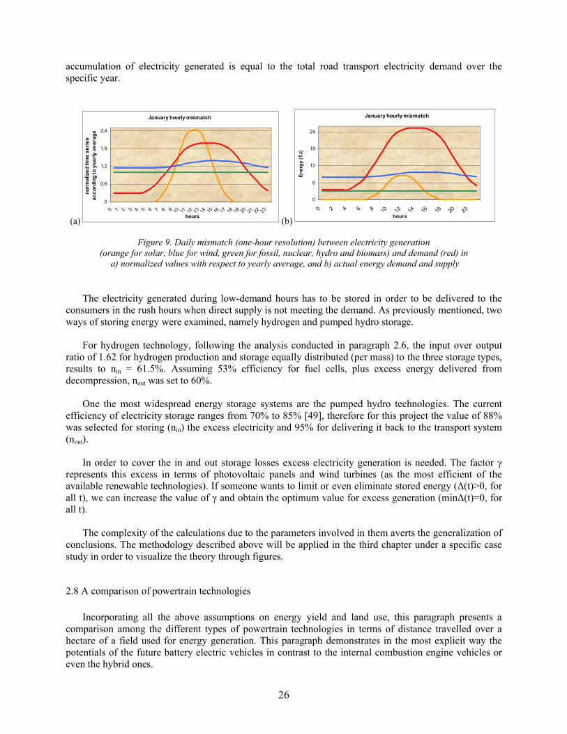
26

accumulation of electricity generated is equal to the total road transport electricity demand over the specific year.

(a)

January hourly mismatch

0

0,6

1,2

1,8

2,4

0 1 2 3 4 5 6 7 8 9 10 11 12 13 14 15 16 17 18 19 20 21 22 23

hours

no

rma

lize

d t

ime

se

rie

s

ac

co

rdin

g t

o y

ea

rly

av

era

ge

(b)

January hourly mismatch

0

6

12

18

24

0 2 4 6 8 10 12 14 16 18 20 22hours

En

erg

y (T

J)

Figure 9. Daily mismatch (one-hour resolution) between electricity generation (orange for solar, blue for wind, green for fossil, nuclear, hydro and biomass) and demand (red) in

a) normalized values with respect to yearly average, and b) actual energy demand and supply

The electricity generated during low-demand hours has to be stored in order to be delivered to the consumers in the rush hours when direct supply is not meeting the demand. As previously mentioned, two ways of storing energy were examined, namely hydrogen and pumped hydro storage.

For hydrogen technology, following the analysis conducted in paragraph 2.6, the input over output ratio of 1.62 for hydrogen production and storage equally distributed (per mass) to the three storage types, results to nin = 61.5%. Assuming 53% efficiency for fuel cells, plus excess energy delivered from decompression, nout was set to 60%.

One the most widespread energy storage systems are the pumped hydro technologies. The current efficiency of electricity storage ranges from 70% to 85% [49], therefore for this project the value of 88% was selected for storing (nin) the excess electricity and 95% for delivering it back to the transport system (nout).

In order to cover the in and out storage losses excess electricity generation is needed. The factor γrepresents this excess in terms of photovoltaic panels and wind turbines (as the most efficient of the available renewable technologies). If someone wants to limit or even eliminate stored energy (Δ(t)>0, for all t), we can increase the value of γ and obtain the optimum value for excess generation (minΔ(t)=0, for all t).

The complexity of the calculations due to the parameters involved in them averts the generalization of conclusions. The methodology described above will be applied in the third chapter under a specific case study in order to visualize the theory through figures.

2.8 A comparison of powertrain technologies

Incorporating all the above assumptions on energy yield and land use, this paragraph presents a comparison among the different types of powertrain technologies in terms of distance travelled over a hectare of a field used for energy generation. This paragraph demonstrates in the most explicit way the potentials of the future battery electric vehicles in contrast to the internal combustion engine vehicles or even the hybrid ones.

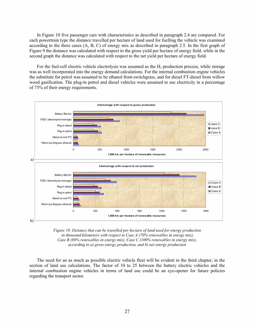
27

In Figure 10 five passenger cars with characteristics as described in paragraph 2.4 are compared. For each powertrain type the distance travelled per hectare of land used for fuelling the vehicle was examined according to the three cases (A, B, C) of energy mix as described in paragraph 2.5. In the first graph of Figure 9 the distance was calculated with respect to the gross yield per hectare of energy field, while in the second graph the distance was calculated with respect to the net yield per hectare of energy field.

For the fuel-cell electric vehicle electrolysis was assumed as the H2 production process, while storage was as well incorporated into the energy demand calculations. For the internal combustion engine vehicles the substitute for petrol was assumed to be ethanol from switchgrass, and for diesel FT-diesel from willow wood gasification. The plug-in petrol and diesel vehicles were assumed to use electricity in a percentage of 75% of their energy requirements.

a)

kilometrage with respect to gross production

0 500 1000 1500 2000 2500

Petrol (sw ithgrass ethanol)

Diesel (w ood FT)

Plug-in petrol

Plug-in diesel

FCEV (electrolysis+storage)

Battery Electric

1,000 km per hectare of renewable resources

case C

case B

Case A

b)

kilometrage with respect to net production

0 300 600 900 1200 1500 1800

Petrol (sw ithgrass ethanol)

Diesel (w ood FT)

Plug-in petrol

Plug-in diesel

FCEV (electrolysis+storage)

Battery Electric

1,000 km per hectare of renewable resources

Case C

Case B

Case A

Figure 10. Distance that can be travelled per hectare of land used for energy production in thousand kilometers with respect to Case A (70% renewables in energy mix),

Case B (80% renewables in energy mix), Case C (100% renewables in energy mix), according to a) gross energy production, and b) net energy production

The need for an as much as possible electric vehicle fleet will be evident in the third chapter, in the section of land use calculations. The factor of 10 to 25 between the battery electric vehicles and the internal combustion engine vehicles in terms of land use could be an eye-opener for future policies regarding the transport sector.

28

3. Calculations

The procedure described in the second chapter produced 9 scenarios on tank-to-wheel energy consumption (three for each of the three fleet composition scenarios), and 27 scenarios on well-to-wheel emissions (three for each of the nine energy consumption scenarios). The calculations on emissions were used to observe under which conditions the road transport sector in the Netherlands can meet the European Commission’s GHG reduction target for 2050, and the calculations on energy consumption to define the amount of land needed, the mismatch and the implications created by each scenario.

3.1 Energy consumption

In Figure 11 the results for the nine tank-to-wheel energy consumption scenarios are presented. The segments in each column represent the energy consumption by fuel type (i.e. electricity, hydrogen, petrol/ethanol, bio-diesel, LPG, CNG). As can be observed, in all three consumption rate scenarios the more the fleet is composed of electric vehicles (hybrid, battery and fuel-cell) the less energy it consumes, and subsequently the less greenhouse gases it emits.

TTW energy consumption

0

150

300

450

ModerateRR2010

ModerateC5a

ModerateScen.III

AverageRR2010

AverageC5a

AverageScen.III

LimitsRR2010

Limits C5a

LimitsScen.III

En

erg

y c

on

su

mp

tio

n (

PJ

)

cng

lpg

(bio)diesel

petrol/ethanol

hydrogen

electricity

Figure 11. Tank-to-wheel energy consumptionunder moderate, average and limits consumption rates

for the three fleet composition scenarios

The total tank-to-wheel annual energy consumption for these nine scenarios ranges from 194PJ (fleet composition: scenario III; consumption rates: limits) to almost 450PJ (fleet composition: RR2010; consumption rates: moderate). The lowest value that can be reached under RR2010 fleet composition scenario is about 360PJ, while under C5a scenario it is about 280PJ (both for “limits” consumption rates).15

In Figure 12 the distribution of passenger car vehicle kilometers based on the different energy carriersfor the ‘RR2010’ fleet composition scenario is illustrated according to the three cases of energy mix (A, B, C).

15 For the exact values see Appendix A.4

29

Passenger cars (RR2010 fleet composition)

0

17.000

34.000

51.000

68.000

petrol ethanol diesel biodiesel cng lpg renew ableelectricity

fossilelectricity

mill

ion

veh

icle

kilo

met

ers

Case A

Case B

Case C

Figure 12. Distribution of vehicle kilometers based on energy carriersfor passenger cars for the RR2010 fleet composition scenario,

according to energy mix cases A, B, and C

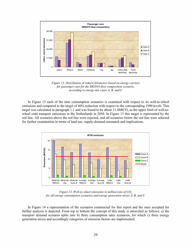
In Figure 13 each of the nine consumption scenarios is examined with respect to its well-to-wheel emissions and compared to the target of 60% reduction with respect to the corresponding 1990 levels. This target was calculated in paragraph 1.1 and was found to be about 11.4MtCO2 as the upper limit of well-to-wheel road transport emissions in the Netherlands in 2050. In Figure 13 this target is represented by the red line. All scenarios above the red line were rejected, and all scenarios below the red line were selected for further examination in terms of land use, supply-demand mismatch and implications.

WTW emissions

0

5

10

15

20

ModerateRR2010

ModerateC5a

ModerateScen.III

AverageRR2010

AverageC5a

AverageScen.III

LimitsRR2010

Limits C5a

LimitsScen.III

Em

iss

ion

s (

MtC

O2

)

Case A

Case B

Case C

target

Figure 13. Well-to-wheel emissions in million tons of CO2

for all energy consumption scenarios and energy generation mixes A, B, and C

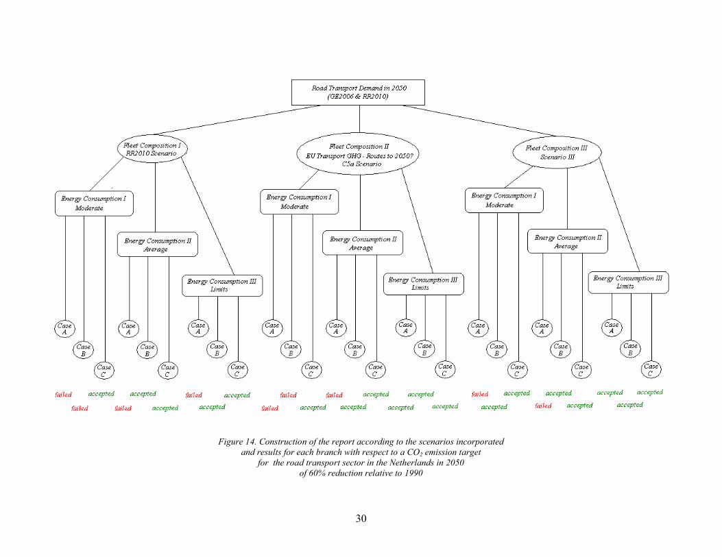
In Figure 14 a representation of the scenarios constructed for this report and the ones accepted for further analysis is depicted. From top to bottom the concept of this study is unraveled as follows: a) the transport demand scenario splits into b) three consumption rates scenarios, for which c) three energy generation mixes and accordingly categories of emission factors are implemented.

30

Figure 14. Construction of the report according to the scenarios incorporated and results for each branch with respect to a CO2 emission target

for the road transport sector in the Netherlands in 2050of 60% reduction relative to 1990

31

3.2 Land use

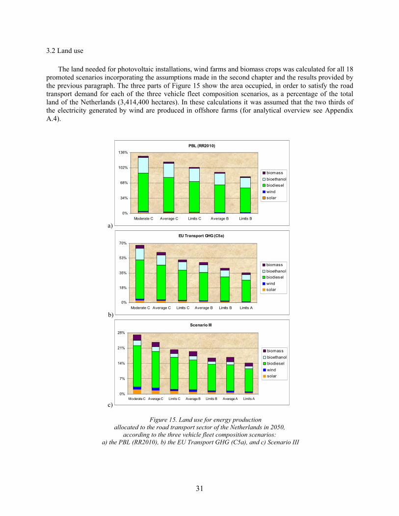
The land needed for photovoltaic installations, wind farms and biomass crops was calculated for all 18 promoted scenarios incorporating the assumptions made in the second chapter and the results provided by the previous paragraph. The three parts of Figure 15 show the area occupied, in order to satisfy the road transport demand for each of the three vehicle fleet composition scenarios, as a percentage of the total land of the Netherlands (3,414,400 hectares). In these calculations it was assumed that the two thirds of the electricity generated by wind are produced in offshore farms (for analytical overview see AppendixA.4).

a)

PBL (RR2010)

0%

34%

68%

102%

136%

Moderate C Average C Limits C Average B Limits B

biomass

bioethanol

biodiesel

wind

solar

b)

EU Transport GHG (C5a)

0%

18%

35%

53%

70%

Moderate C Average C Limits C Average B Limits B Limits A

biomass

bioethanol

biodiesel

wind

solar

c)

Scenario III

0%

7%

14%

21%

28%

Moderate C Average C Limits C Average B Limits B Average A Limits A

biomass

bioethanol

biodiesel

wind

solar

Figure 15. Land use for energy production allocated to the road transport sector of the Netherlands in 2050,

according to the three vehicle fleet composition scenarios: a) the PBL (RR2010), b) the EU Transport GHG (C5a), and c) Scenario III

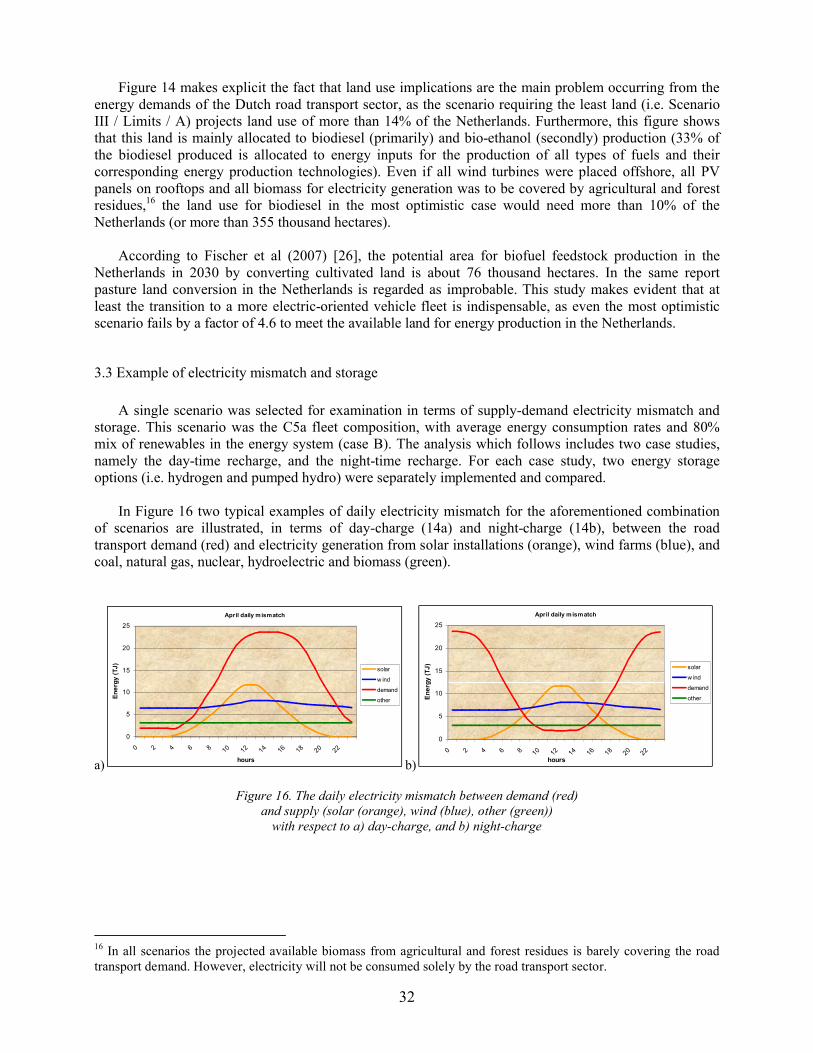
32

Figure 14 makes explicit the fact that land use implications are the main problem occurring from the energy demands of the Dutch road transport sector, as the scenario requiring the least land (i.e. Scenario III / Limits / A) projects land use of more than 14% of the Netherlands. Furthermore, this figure shows that this land is mainly allocated to biodiesel (primarily) and bio-ethanol (secondly) production (33% of the biodiesel produced is allocated to energy inputs for the production of all types of fuels and their corresponding energy production technologies). Even if all wind turbines were placed offshore, all PV panels on rooftops and all biomass for electricity generation was to be covered by agricultural and forest residues,16 the land use for biodiesel in the most optimistic case would need more than 10% of the Netherlands (or more than 355 thousand hectares).

According to Fischer et al (2007) [26], the potential area for biofuel feedstock production in the Netherlands in 2030 by converting cultivated land is about 76 thousand hectares. In the same report pasture land conversion in the Netherlands is regarded as improbable. This study makes evident that at least the transition to a more electric-oriented vehicle fleet is indispensable, as even the most optimistic scenario fails by a factor of 4.6 to meet the available land for energy production in the Netherlands.

3.3 Example of electricity mismatch and storage

A single scenario was selected for examination in terms of supply-demand electricity mismatch and storage. This scenario was the C5a fleet composition, with average energy consumption rates and 80% mix of renewables in the energy system (case B). The analysis which follows includes two case studies, namely the day-time recharge, and the night-time recharge. For each case study, two energy storage options (i.e. hydrogen and pumped hydro) were separately implemented and compared.

In Figure 16 two typical examples of daily electricity mismatch for the aforementioned combination of scenarios are illustrated, in terms of day-charge (14a) and night-charge (14b), between the road transport demand (red) and electricity generation from solar installations (orange), wind farms (blue), and coal, natural gas, nuclear, hydroelectric and biomass (green).

a)

April daily mismatch

0

5

10

15

20

25

0 2 4 6 8 10 12 14 16 18 20 22

hours

En

erg

y (

TJ

)

solar

w ind

demand

other

b)

April daily mismatch

0

5

10

15

20

25

0 2 4 6 8 10 12 14 16 18 20 22hours

En

erg

y (

TJ

) solar

w ind

demand

other

Figure 16. The daily electricity mismatch between demand (red) and supply (solar (orange), wind (blue), other (green))

with respect to a) day-charge, and b) night-charge

16 In all scenarios the projected available biomass from agricultural and forest residues is barely covering the road transport demand. However, electricity will not be consumed solely by the road transport sector.

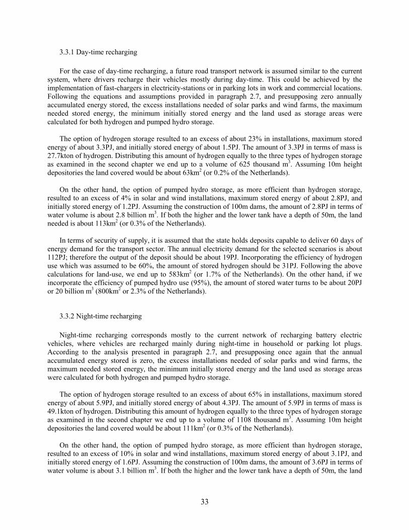
33

3.3.1 Day-time recharging

For the case of day-time recharging, a future road transport network is assumed similar to the current system, where drivers recharge their vehicles mostly during day-time. This could be achieved by the implementation of fast-chargers in electricity-stations or in parking lots in work and commercial locations.Following the equations and assumptions provided in paragraph 2.7, and presupposing zero annually accumulated energy stored, the excess installations needed of solar parks and wind farms, the maximum needed stored energy, the minimum initially stored energy and the land used as storage areas were calculated for both hydrogen and pumped hydro storage.

The option of hydrogen storage resulted to an excess of about 23% in installations, maximum stored energy of about 3.3PJ, and initially stored energy of about 1.5PJ. The amount of 3.3PJ in terms of mass is 27.7kton of hydrogen. Distributing this amount of hydrogen equally to the three types of hydrogen storage as examined in the second chapter we end up to a volume of 625 thousand m3. Assuming 10m height depositories the land covered would be about 63km2 (or 0.2% of the Netherlands).

On the other hand, the option of pumped hydro storage, as more efficient than hydrogen storage, resulted to an excess of 4% in solar and wind installations, maximum stored energy of about 2.8PJ, and initially stored energy of 1.2PJ. Assuming the construction of 100m dams, the amount of 2.8PJ in terms of water volume is about 2.8 billion m3. If both the higher and the lower tank have a depth of 50m, the land needed is about 113km2 (or 0.3% of the Netherlands).

In terms of security of supply, it is assumed that the state holds deposits capable to deliver 60 days of energy demand for the transport sector. The annual electricity demand for the selected scenarios is about 112PJ; therefore the output of the deposit should be about 19PJ. Incorporating the efficiency of hydrogen use which was assumed to be 60%, the amount of stored hydrogen should be 31PJ. Following the above calculations for land-use, we end up to 583km2 (or 1.7% of the Netherlands). On the other hand, if we incorporate the efficiency of pumped hydro use (95%), the amount of stored water turns to be about 20PJor 20 billion m3 (800km2 or 2.3% of the Netherlands).

3.3.2 Night-time recharging

Night-time recharging corresponds mostly to the current network of recharging battery electric vehicles, where vehicles are recharged mainly during night-time in household or parking lot plugs. According to the analysis presented in paragraph 2.7, and presupposing once again that the annual accumulated energy stored is zero, the excess installations needed of solar parks and wind farms, the maximum needed stored energy, the minimum initially stored energy and the land used as storage areas were calculated for both hydrogen and pumped hydro storage.

The option of hydrogen storage resulted to an excess of about 65% in installations, maximum stored energy of about 5.9PJ, and initially stored energy of about 4.3PJ. The amount of 5.9PJ in terms of mass is 49.1kton of hydrogen. Distributing this amount of hydrogen equally to the three types of hydrogen storage as examined in the second chapter we end up to a volume of 1108 thousand m3. Assuming 10m height depositories the land covered would be about 111km2 (or 0.3% of the Netherlands).

On the other hand, the option of pumped hydro storage, as more efficient than hydrogen storage, resulted to an excess of 10% in solar and wind installations, maximum stored energy of about 3.1PJ, and initially stored energy of 1.6PJ. Assuming the construction of 100m dams, the amount of 3.6PJ in terms of water volume is about 3.1 billion m3. If both the higher and the lower tank have a depth of 50m, the land

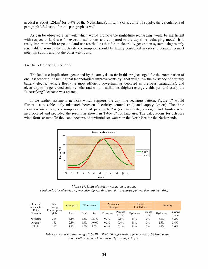
34

needed is about 126km2 (or 0.4% of the Netherlands). In terms of security of supply, the calculations of paragraph 3.3.1 stand for this paragraph as well.

As can be observed a network which would promote the night-time recharging would be inefficient with respect to land use for excess installations and compared to the day-time recharging model. It is really important with respect to land-use restrictions that for an electricity generation system using mainly renewable resources the electricity consumption should be highly controlled in order to demand to meet potential supply and not the other way round.

3.4 The “electrifying” scenario

The land-use implications generated by the analysis so far in this project urged for the examination ofone last scenario. Assuming that technological improvements by 2050 will allow the existence of a totally battery electric vehicle fleet (the most efficient powertrain as depicted in previous paragraphs), and electricity to be generated only by solar and wind installations (highest energy yields per land used), the “electrifying” scenario was created.

If we further assume a network which supports the day-time recharge pattern, Figure 17 would illustrate a possible daily mismatch between electricity demand (red) and supply (green). The three scenarios on energy consumption rates of paragraph 2.4 (i.e. moderate, average, and limits) were incorporated and provided the results as shown in Table 17 for land use. The calculations for offshore wind-farms assume 76 thousand hectares of territorial sea waters in the North Sea for the Netherlands.

August daily mismatch

0

7

14

21

28

0 2 4 6 8 10 12 14 16 18 20 22

hours

En

erg

y (T

J)

supply

demand

Figure 17. Daily electricity mismatch assuming wind and solar electricity generation (green line) and day-recharge pattern demand (red line)

Solar-parks Wind-farmsMismatchStorage

ExcessInstallations

SecurityEnergy

Consumption Rates

Scenario

Total Energy

Consumption(PJ) Land Land Sea Hydrogen

Pumped Hydro

HydrogenPumped Hydro

HydrogenPumped Hydro

Moderate 200 3.1% 1.6% 12.3% 0.3% 0.5% 18% 3% 3.1% 4.2%

Average 162 2.5% 1.3% 10.0% 0.2% 0.4% 18% 3% 2.5% 3.4%

Limits 123 1.9% 1.0% 7.6% 0.2% 0.4% 18% 3% 1.9% 2.6%

Table 17. Land use assuming 100% BEV fleet, 60% generation from wind, 40% from solar and monthly mismatch stored in H2 or pumped hydro

35

As can be observed the land use implications are still significant even in the most optimistic case of the ‘Limits’ consumption rates scenario, in which more than 5% of the Netherlands is needed to fuel the road transport sector and about 8% of the territorial sea waters of the country. Here one needs to mention that the road transport sector consumes only about one fifth of the total energy consumed in the Netherlands and that other sectors have even higher GHG reduction targets as part of the European ambition for 2050.

36

4. Conclusions

In this project the availability of renewable resources for the road transport sector in the Netherlands in 2050 was examined by developing several scenarios with respect to fleet composition, consumption rates, energy mix, recharging patterns and storage solutions. What became evident from the results obtained were the severe implications in terms of land use. Even by reaching the limits of technological improvements and assuming rapid and radical changes in vehicle market and energy generation patterns, the road transport sector is still kept far from sustainable levels.

The scenarios developed in this report were based on two studies, the WLO and the most recent PBL data for the future road transport demand in the Netherlands. Consequently, three vehicle energy efficiency scenarios were constructed; the first two using the PBL data and a policy scenario developed inthe report “EU Transport GHG: Routes to 2050?”, and the third expanding efficiency to its limits. Further on, three cases for the fuel mix and the electricity generation were made, resulting in total to 27 scenarios on carbon emissions.

As shown in this project the European Commission target for CO2 emissions reduction of 60% by 2050 in the road transport sector of the Netherlands with reference to the 1990 levels is feasible under certain conditions; first of all the shift of the transport fleet composition from combustion engine vehicles to hybrid and electric vehicles, secondly the improvements in energy efficiency of the vehicles and the supply system, and thirdly the decarbonisation of the energy supply system and especially the electricity generation sector.

The annual tank-to-wheel energy requirements for the scenarios which meet the EC targets are spanning from 200PJ –for the extreme case of fleet shift and efficiency reaching the limits– to 450PJ –for the business as usual fleet composition scenario with moderate efficiency improvements. Even though the TTW energy consumption was found to be lower than the contemporary consumption of the road transport sector, the implications with the land used for the production of combustible fuels and electricity generation are apparent.

The most optimistic scenario is employing 14% of land (74% of it used for biodiesel production) and 4% of territorial sea waters of the Netherlands only for the road transport sector. Even without regarding that the road transport sector consumes one fifth of the energy used in the Netherlands, the land use implications are vast. A solution largely discussed promotes the use of foreign energy resources; however, this scenario contradicts with the very essence of sustainability in terms of self-sustenance. Moreover, the security of supply would be a crucial matter as the demand is large enough to render the Netherlands dependent on foreign relations and global changes, as is in fact nowadays the case with fossil fuels.

What is common in all scenarios developed in this project is the projection on road transport demand. Based on the PBL and WLO business-as-usual data the demand for passenger car and truck kilometreswill keep increasing. Even under conditions of severe change in market trends and large and fast technological improvements, the road transport sector of the Netherlands in 2050 will not be able to meet the levels of sustainability. Therefore, the transition needed seems to be on the demand growth.

Many scientists and philosophers around the world raise concerns on the limits to growth with respect to consumption, economic development, lifestyle, urbanization, the political structure of our societies and so on [50][51]. The multiple crises which strike on a global scale in the recent years confirm the need for a shift in mentality, and the de-growth theory reaches more and more correspondence to the scientific and non-scientific populace.17

17 See for example the documentary “Homage to Catalonia II”, available on http://www.homenatgeacatalunyaii.org/en

37

The term ‘de-growth’ does not correspond to negative growth, but rather to sensible growth. For instance, in the road transport sector, which was the subject of this project, along with technological improvements the need for modal change and decrease of transport demand is evident. By the term “modal change” it is suggested the shift from personal to public transportation and if possible to walking and cycling (though in the Netherlands the latter one is already a part of the lifestyle). The decrease in transport demand could be achieved by implementing several combinations of scenarios like localization of production and consumption in terms of food, goods and energy, limiting commuting to work and restructuring urban areas.

A sustainable world is possible. Technology can be a part of the solution; however it is not a panacea.

38

References

[1] Source: www.pbl.nl (Internal communication with Anco Hoen. Report retrieved from: http://www.pbl.nl/sites/default/files/pdfs/Referentieraming_en_Milieueffecten_WEB.pdf)

[2] International Energy Agency website: http://www.iea.org/[3] Smokers, R. Vermeulen, R. van Mieghem, R. Gense, R. Skinner, I. Fergusson, M. MacKay, E. ten

Brink, P. Fontaras, G. Samaras, Z. (2006), Review and analysis of the reduction potential and costs of technological and other measures to reduce CO2-emissions from passenger cars, Table 6.4, TNO, IEEP, LAT

[4] European Commission (2011) White Paper on Transport (retrieved from : http://ec.europa.eu/transport/strategies/2011_white_paper_en.htm)

[5] World Bank Indicators on Transport (source: http://www.tradingeconomics.com/netherlands/passenger-cars-per-1-000-people-wb-data.html)

[6] Thomas, C.E. (2009), ‘Fuel cell and battery electric vehicles compared’, International Journal of Hydrogen Energy 34 (2009) 6005-6020

[7] Ross, M. (1997), ‘Fuel Efficiency and the Physics of Automobiles’, Contemporary Physics 38, no.6 (1997) 381-394

[8] The American Institute of Physics web-page http://www.aip.org/tip/INPHFA/vol-10/iss-1/p20.html

[9] Eliasson, B. & Bossel, U (2000), The Future of the Hydrogen Economy, ABB Switzerland Ltd[10] Graus, W. & Worrell, E. (2011) Methods for calculating CO2 intensity of power generation and

consumption: A global perspective, Energy Policy 39 (2011) 613-627[11] Van Harmelen, A.K. Koch, W.R.R. (2002) CO2 emission factors for fuels in the Netherlands,

TNO, Apeldoorn, The Netherlands[12] Koornneef, J. van Harmelen, T. van Horssen, A. van Gijlswijk, R Ramirez, A. Faaij, A

Turkenburg, W. (2009) The impacts of CO2 capture on transboundary air pollution in the Netherlands, Energy Procedia 1 (2009) 3787-3794

[13] European Commission (2010) EU energy and transport in figures 2010, Publications Office of the European Union, Luxembourg

[14] International Energy Agency (2010) CO2 emissions from fuel combustion – Highlights, IEA, Paris[15] Energy research Centre of the Netherlands (2011) Nuclear energy facts, ECN, 18 March 2011[16] Market Observatory for Energy (2010) Netherlands, European Commission & DG Energy[17] http://ec.europa.eu/energy/energy_policy/doc/factsheets/mix/mix_nl_en.pdf[18] Hoen, A. van den Brink, R.M.M. Annema J.A. (2006), Verkeer en vervoer in de Welvaart en

Leefomgeving – Achtergronddocument bij Emissieprognoses Verkeer en Vervoer, MNP rapport 500076002/2006

[19] Hoen, A. Kieboom, S.F. Geilenkirchen, G.P. Hanschke, C.B. (2010) Verkeer en vervoer in de Referentieraming Energie en Emissies 2010-2020 – Broeikasgassen en luchtverontreinigende stoffen, Den Haag/Bilthoven (retrieved from: http://www.pbl.nl/publicaties/2010/Verkeer-en-vervoer-de-Referentieraming-Energie-en-Emissies-2010-2020-Broeikasgassen-en-luchtverontreinigende-st)

[20] Borjesson, P. & Tufvesson, L.M. (2011), Agricultural crop-based biofuels – resource efficiency and environmental performance including direct land use changes, Journal of Cleaner Production 19 (2011) 108-120

[21] Dijkman, T.J. & Benders, R.M.J. (2010), Comparison of renewable fuels based on their land use using energy densities, Renewable and Sustainable Energy Reviews 14 (2010) 3148-3155

[22] Pimentel, D. & Patzek, T.W. (2005), Ethanol Production Using Corn, Switchgrass, and Wood; Biodiesel Production Using Soybean and Sunflower, Natural Resources Research, Vol. 14, No. 1, March 2005

39

[23] International Energy Agency (2010), ‘Sustainable Production of Second-Generation Biofuels – Potential and perspectives in major economies and developing countries’, Paris, France

[24] Boerrigter, H. (2002) ‘Green’ Diesel Production with Fischer-Tropsch Synthesis, Business Meeting Bio-Energy; Platform Bio-Energie, 13 September 2002

[25] Opdal, O.A. (2006) Production of synthetic biodiesel via Fischer-Tropsch synthesis – Biomass-to-liquids in Namdalen, Norway, Norwegian University of Science and Technology, Trondheim(retrieved from: http://www.zero.no/transport/biodrivstoff/btl-namdalen.pdf)

[26] Fischer, G. Hizsnyik, E. Prieler, S. van Velthuizen, H. (2007), Assessment of biomass potentials for biofuel feedstock production in Europe: Methodology and results, IIASA (retrieved from: http://www.refuel.eu/uploads/media/Refuel-D6-Jul2007-final6.pdf)

[27] Bai, Y. Luo, L. & van der Voet, E. (2010), Life cycle assessment of switchgrass-derived ethanol as transport fuel, Int J Life Cycle Assess (2010) 15: 468-477

[28] Food and Agriculture Organization of the United Nations, Statistics Division web-pagehttp://faostat.fao.org/

[29] Larsson, M. and Norden, B. (1982) Compacting of Tree Sections from Clear Cuttings with Separate Equipment, Report no 1982-10-01. Forskningsstifelsen, Skogsarbeten, Sweden

[30] Environmental research Centre of the Netherlands, Phyllis web page http://www.ecn.nl/phyllis/[31] Jungbluth, N. Tuchschmid, M. de Wild-Scholten, M. (2008), Life Cycle Assessment of

Photovoltaics: Update of ecoinvent data v2.0, ESU-services Ltd http://www.esu-services.ch/[32] Kaplanis, S. Kaplani, E. (2011), Energy performance and degradation over 20 years performance

of BP c-Si PV modules, Simulation Modelling Practice and Theory 19 (2011) 1201-1211[33] European Wind Energy Association (2009), Wind Energy – The Facts, retrieved from:

http://www.wind-energy-the-facts.org/[34] Brand, A.J. (2008), Offshore wind atlas of the Dutch part of the North Sea, ECN[35] Hu, Y. Weimer, C. (2009), Global high resolution wind speed statistics from satellite lidar

measurement, Joint Office for Science Support (retrieved from: http://www.joss.ucar.edu/events/2010/seaflux/abstracts/HuYongxiangAbstract.pdf)

[36] Meyers, J. and Meneveau, C. (2011), Optimal turbine spacing in fully developed wind farm boundary layers, Wind Energy, 14: n/a. doi: 10.1002/we.469

[37] Crawford, R.H. (2009), Life cycle energy and greenhouse emissions analysis of wind turbines and the effect of size on energy yield, Renewable and Sustainable Energy Reviews 13 (2009), 2653-2660

[38] The British Wind Energy Association (2005), Blowing Away the Myths – A critique of the Renewable Energy Foundation’s report: Reduction in carbon dioxide emissions: estimating the potential contribution from wind power, London, UK (retrieved from: http://www.bwea.com/pdf/ref_three.pdf)

[39] Heide, D. von Bremen, L. Greiner, M. Hoffmann, C. Speckmann, M. Bofinger, S. (2010)Seasonal optimal mix of wind and solar power in a future, highly renewable Europe, Renewable Energy 35 (2010) 2483-2489

[40] Kroposki, B. Levene, J. Harrison, K. (2006) Electrolysis: Information and Opportunities for Electric Power Utilities, National Renewable Energy Laboratory, Colorado, USA (retrieved from: http://www.nrel.gov/docs/fy06osti/40605.pdf)

[41] Meza, J. Gil, A, Cortes, C. Gonzalez, A. (2008), Drying costs of woody biomass in a semi-industrial experimental rotary dryer’, CIRCE, 16th European Conference & Exhibition on Biomass for Energy, Biomass Resources, 2-6 June 2008, Valencia, Spain

[42] U.S. Department of Energy, Energy Efficiency & Renewable Energy, Hydrogen Storage(http://www1.eere.energy.gov/hydrogenandfuelcells/storage/hydrogen_storage.html?m=1&)

[43] Presentation (2010) Opportunities in the Pipeline: Latest Developments in Carbon Capture and Storage, Sustainable Energy Futures Conference 2010, Imperial College London (retrieved from: http://workspace.imperial.ac.uk/energyfutureslab/Public/SEF%20conference%20presentations/4.%20CCS.pdf)

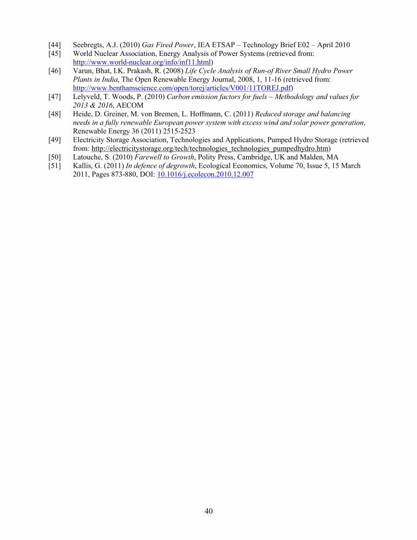
40

[44] Seebregts, A.J. (2010) Gas Fired Power, IEA ETSAP – Technology Brief E02 – April 2010[45] World Nuclear Association, Energy Analysis of Power Systems (retrieved from:

http://www.world-nuclear.org/info/inf11.html)[46] Varun, Bhat, I.K. Prakash, R. (2008) Life Cycle Analysis of Run-of River Small Hydro Power

Plants in India, The Open Renewable Energy Journal, 2008, 1, 11-16 (retrieved from: http://www.benthamscience.com/open/torej/articles/V001/11TOREJ.pdf)

[47] Lelyveld, T. Woods, P. (2010) Carbon emission factors for fuels – Methodology and values for 2013 & 2016, AECOM

[48] Heide, D. Greiner, M. von Bremen, L. Hoffmann, C. (2011) Reduced storage and balancing needs in a fully renewable European power system with excess wind and solar power generation, Renewable Energy 36 (2011) 2515-2523

[49] Electricity Storage Association, Technologies and Applications, Pumped Hydro Storage (retrieved from: http://electricitystorage.org/tech/technologies_technologies_pumpedhydro.htm)

[50] Latouche, S. (2010) Farewell to Growth, Polity Press, Cambridge, UK and Malden, MA[51] Kallis, G. (2011) In defence of degrowth, Ecological Economics, Volume 70, Issue 5, 15 March

2011, Pages 873-880, DOI: 10.1016/j.ecolecon.2010.12.007

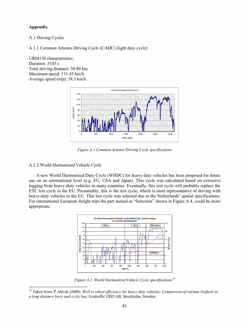
41

Appendix

A.1 Driving Cycles

A.1.1 Common Artemis Driving Cycle (CADC) (light duty cycle)

URM130 characteristics:Duration: 3143 sTotal driving distance: 50.89 kmMaximum speed: 131.43 km/hAverage speed (trip): 58.3 km/h

Artemis European Driving Cycle

0

20

40

60

80

100

120

140

0 500 1000 1500 2000 2500 3000

time (sec)

spee

d (k

m/h

)

Figure A.1 Common Artemis Driving Cycle specifications

A.1.2 World Harmonized Vehicle Cycle

A new World Harmonized Duty Cycle (WHDC) for heavy duty vehicles has been proposed for future use on an international level (e.g. EU, USA and Japan). This cycle was calculated based on extensive logging from heavy-duty vehicles in many countries. Eventually, this test cycle will probably replace the ETC test cycle in the EU. Presumably, this is the test cycle, which is most representative of driving with heavy-duty vehicles in the EU. This test cycle was selected due to the Netherlands’ spatial specifications. For international European freight trips the part named as “Selection” shown in Figure A.4, could be more appropriate.

Figure A.2. World Harmonized Vehicle Cycle specifications18

18 Taken from: P.Ahlvik (2008), Well to wheel efficiency for heavy duty vehicles: Comparison of various biofuels in a long distance lorry and a city bus, Ecotraffic ERD AB, Stockholm, Sweden

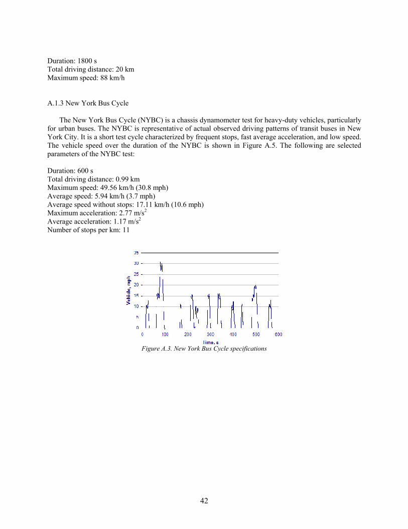
42

Duration: 1800 sTotal driving distance: 20 kmMaximum speed: 88 km/h

A.1.3 New York Bus Cycle

The New York Bus Cycle (NYBC) is a chassis dynamometer test for heavy-duty vehicles, particularly for urban buses. The NYBC is representative of actual observed driving patterns of transit buses in New York City. It is a short test cycle characterized by frequent stops, fast average acceleration, and low speed. The vehicle speed over the duration of the NYBC is shown in Figure A.5. The following are selected parameters of the NYBC test:

Duration: 600 s Total driving distance: 0.99 km Maximum speed: 49.56 km/h (30.8 mph) Average speed: 5.94 km/h (3.7 mph) Average speed without stops: 17.11 km/h (10.6 mph) Maximum acceleration: 2.77 m/s2

Average acceleration: 1.17 m/s2

Number of stops per km: 11

Figure A.3. New York Bus Cycle specifications

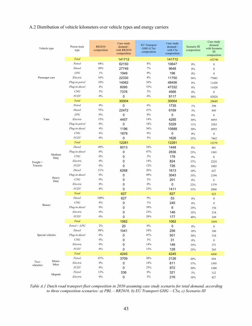
43

A.2 Distribution of vehicle kilometers over vehicle types and energy carriers

Vehicle typePower-train

typeRR2010

composition

Case studydemand -

with RR2010composition

EU Transport GHG (C5a)composition

Case studydemand -with C5a

composition

Scenario IIIcomposition

Case studydemand

with Scenario III

compositionTotal 141712 141712 142746Petrol 44% 62150 8% 10647 0% 0Diesel 20% 27749 7% 9648 0% 0LPG 1% 1949 0% 196 0% 0

Electric 16% 22330 8% 11750 54% 77083Plug-in petrol 10% 14062 34% 48456 8% 11420Plug-in diesel 4% 6095 33% 47332 8% 11420

CNG 5% 7376 3% 4566 0% 0

Passenger cars

FCEV 0% 0 6% 9117 30% 42824Total 30004 30004 29849Petrol 0% 0 6% 1735 1% 298Diesel 75% 22472 21% 6169 3% 895LPG 0% 0 0% 0 0% 0

Electric 15% 4457 14% 4285 30% 8955Plug-in petrol 0% 0 18% 5329 11% 3283Plug-in diesel 4% 1196 36% 10888 30% 8955

CNG 6% 1879 0% 0 0% 0

Vans

FCEV 0% 0 5% 1626 25% 7462Total 12281 12281 12279Diesel 49% 6013 24% 1448 8% 481

Plug-in diesel 0% 0 47% 2836 25% 1503CNG 0% 0 3% 178 0% 0

Electric 0% 0 14% 824 37% 2224

Medium Duty

FCEV 0% 0 12% 726 30% 1803Diesel 51% 6268 26% 1613 10% 627

Plug-in diesel 0% 0 49% 3043 35% 2194CNG 0% 0 3% 201 0% 0

Electric 0% 0 0% 0 22% 1379

Freight +Tractors

Heavy Duty

FCEV 0% 0 23% 1411 33% 2068Total 627 627 623Diesel 100% 627 9% 53 0% 0CNG 0% 0 1% 245 0% 0

Plug-in diesel 0% 0 39% 6 25% 156Electric 0% 0 23% 146 35% 218

Busses

FCEV 0% 0 28% 177 40% 249Total 1062 1062 1059

Petrol + LPG 2% 20 0% 0 0% 0Diesel 98% 1041 24% 256 10% 106

Plug-in diesel 0% 0 47% 501 30% 318CNG 0% 0 3% 31 0% 0

Electric 0% 0 14% 146 35% 371

Special vehicles

FCEV 0% 0 12% 128 25% 265Total 4245 4245 4268Petrol 87% 3709 50% 2126 20% 854

Electric 0% 0 14% 611 37% 1595Motor-bikes

FCEV 0% 0 23% 972 30% 1280Petrol 13% 536 8% 321 3% 112

Two-wheelers

MopedsElectric 0% 0 5% 216 10% 427

Table A.1 Dutch road transport fleet composition in 2050 assuming case study scenario for total demand, according to three composition scenarios: a) PBL – RR2010, b) EU Transport GHG – C5a, c) Scenario III

44

A.3 Natural Limits of Solar Cell Efficiency

The different semiconductor materials or combinations are suited only for specific spectral ranges. Therefore a specific portion of the radiant energy cannot be used, because the light quanta (photons) do not have enough energy to "activate" the charge carriers. Moreover, a certain amount of surplus photon energy is transformed into heat rather than into electrical energy. In addition to that, there are optical losses, such as the shadowing of the cell surface through contact with the glass surface or reflection of incoming rays on the cell surface. Other loss mechanisms are electrical resistance losses in the semiconductor and the connecting cable. The disrupting influence of material contamination, surface effects and crystal defects, however, are also significant. Single loss mechanisms (photons with too little energy are not absorbed, surplus photon energy is transformed into heat) cannot be further improved because of inherent physical limits imposed by the materials themselves. This leads to a theoretical maximum level of efficiency, i.e. approximately 28% for crystal silicon.

Figure A.1. Theoretical maximum levels of efficiency of various solar cells at standard conditions

45

A.4 Energy Consumption and Land Use

Fleet Composition

Consumption Rate

Electricity Hydrogen Petrol / Ethanol Diesel / FT LPG CNG Total

moderate 39 0 123 264 3 20 449

average 32 0 112 239 3 18 404PBL

(RR2010)limits 25 0 101 214 3 16 359

moderate 137 34 47 141 0 13 374

average 112 19 41 125 0 12 310EU

Transport GHG (C5a) limits 86 21 35 109 0 11 263

moderate 124 96 9 57 0 0 285

average 102 53 8 50 0 0 213Scenario

IIIlimits 80 64 6 44 0 0 194

Table A.2 Total tank-to-wheel energy consumption by powertrain technology for each of the three fleet composition scenarios

Land SeaFleet

CompositionConsumption

RateEnergy

Mix Total SolarWind

(inland)Bio-diesel(willow)

Bio-ethanol(switchgrass)

Biomass(willow)

Wind(offshore)

Moderate C 128% 2.9% 1.5% 85.3% 35.1% 3.2% 12%

Average C 115% 1.9% 1.0% 77.0% 32.2% 2.7% 8%

Limits C 103% 1.6% 0.9% 68.8% 28.9% 2.4% 7%

PBL(RR2010)

Limits B 82% 0.8% 0.6% 55.0% 23.1% 1.9% 5%

Moderate C 68% 2.8% 1.5% 46.1% 13.6% 3.5% 12%

Average C 59% 2.4% 1.3% 40.8% 11.8% 2.9% 10%

Limits C 51% 1.9% 1.0% 35.5% 9.9% 2.3% 8%

Moderate B 54% 1.8% 1.2% 37.3% 10.9% 3.2% 9%

Average B 48% 1.5% 1.0% 32.9% 9.5% 2.7% 8%

EU Transport

GHG (C5a)

Limits B 41% 1.2% 0.8% 28.6% 7.9% 2.2% 6%

Moderate C 27% 2.1% 1.1% 18.8% 2.6% 2.5% 9%

Average C 24% 1.8% 1.0% 16.7% 2.2% 2.1% 7%

Limits C 20% 1.4% 0.8% 14.6% 1.7% 1.7% 6%

Moderate B 22% 1.4% 1.0% 15.4% 2.1% 2.4% 7%

Average B 19% 1.2% 0.8% 13.7% 1.7% 2.0% 6%

Limits B 16% 0.9% 0.6% 11.9% 1.4% 1.6% 5%

Average A 17% 0.7% 0.6% 11.9% 1.5% 1.9% 5%

Scenario III

Limits A 14% 0.6% 0.5% 10.4% 1.2% 1.5% 4%

Table A.3 Land use and territorial sea waters area use for the three fleet composition scenarios