A PRINCIPAL INVESTIGATION OF THE GROUP VELOCITY DISPERSION (GVD) PROFILE FOR OPTIMUM DISPERSION...
16
Progress In Electromagnetics Research, PIER 75, 209–224, 2007 A PRINCIPAL INVESTIGATION OF THE GROUP VELOCITY DISPERSION (GVD) PROFILE FOR OPTIMUM DISPERSION COMPENSATION IN OPTICAL FIBERS: A THEORETICAL STUDY A. Rostami Photonics and Nanocrystal Research Lab. Faculty of Electrical and Computer Engineering University of Tabriz Tabriz 51664, Iran A. Andalib Department of Electrical Engineering Islamic Azad University of Science and Technology Tehran, Iran Abstract—In this paper, an analytical method for management of optimum group velocity dispersion (GVD) for compensation of chromatic dispersion in optical fibers is proposed. The proposed method mathematically is based on the Volterra series as alternative method for solution of the nonlinear Schr¨ odinger equation (NLS). Based on analytical solution of the nonlinear equation in pulse propagation, we propose a differential equation including optimum GVD for complete dispersion compensation for given dispersion coefficient and fiber length. The obtained integro-differential equation is solved for special cases and it is shown that the obtained results are so better than traditional dispersion compensation cases. Also, the proposed technique can be applied to fiber design to introduce an especial GVD profile for dispersion less transmission. 1. INTRODUCTION Optical fiber is physical medium for realization of optical communi- cation algorithms which is one of acceptable and interesting methods recently for data communications. There are two main problems in this physical medium that are dispersion and power loss. Selection of
-
Upload
independent -
Category
Documents
-
view
2 -
download
0
Transcript of A PRINCIPAL INVESTIGATION OF THE GROUP VELOCITY DISPERSION (GVD) PROFILE FOR OPTIMUM DISPERSION...

Progress In Electromagnetics Research, PIER 75, 209–224, 2007
A PRINCIPAL INVESTIGATION OF THE GROUPVELOCITY DISPERSION (GVD) PROFILE FOROPTIMUM DISPERSION COMPENSATION INOPTICAL FIBERS: A THEORETICAL STUDY
A. Rostami
Photonics and Nanocrystal Research Lab.Faculty of Electrical and Computer EngineeringUniversity of TabrizTabriz 51664, Iran
A. Andalib
Department of Electrical EngineeringIslamic Azad University of Science and TechnologyTehran, Iran
Abstract—In this paper, an analytical method for managementof optimum group velocity dispersion (GVD) for compensation ofchromatic dispersion in optical fibers is proposed. The proposedmethod mathematically is based on the Volterra series as alternativemethod for solution of the nonlinear Schrodinger equation (NLS).Based on analytical solution of the nonlinear equation in pulsepropagation, we propose a differential equation including optimumGVD for complete dispersion compensation for given dispersioncoefficient and fiber length. The obtained integro-differential equationis solved for special cases and it is shown that the obtained resultsare so better than traditional dispersion compensation cases. Also,the proposed technique can be applied to fiber design to introduce anespecial GVD profile for dispersion less transmission.
1. INTRODUCTION
Optical fiber is physical medium for realization of optical communi-cation algorithms which is one of acceptable and interesting methodsrecently for data communications. There are two main problems inthis physical medium that are dispersion and power loss. Selection of

210 Rostami and Andalib
suitable carrier wavelength such as 1.55 um corresponding to minimumloss of common optical fibers really can be removed the loss problemof this physical medium for light propagation. Also, Erbium dopedfiber amplifiers (EDFA) which are completely compatible with fiberscan be used to compensate optical loss through propagation. The sec-ond and important problem is dispersion effect. Complete solution forthis problem doesn’t exist. There are huge proposals for dispersioncompensation which in the following we review some of them brieflyand discuss advantages and disadvantages.
Pre-chirping is one of common methods for dispersion compensa-tion [1, 2]. Minus chirping in the case of positive GVD introduces pulsecompression and can be used as dispersion compensator which is tryto broad optical pulse. Digital modulation such as frequency shiftedkeying (FSK) is another method for dispersion compensation [3–5].Nonlinear pre-chirping is another method for dispersion compensation[6, 7]. In this method semiconductor optical amplifier is used in thesaturation region. Also, some post dispersion compensation methodswere used. One of common method in this category is dispersion com-pensating fibers [8–11]. In this method fiber with negative dispersionin given wavelength which basic fibers have positive values is used tocompensate pulse broadening.
Optical fibers with given phase dependency on frequency isanother method for dispersion compensation of optical fibers [1, 12, 15].Fiber Bragg Grating is another method for dispersion compensatingin optical fibers [16–18]. Using the parameters used in Bragg gratingfrequency response of this structure can be managed and dispersioncompensation can be done. Optical phase conjugation can be usedfor dispersion compensation also [19]. Finally a more commonmethod named dispersion management technique is used for dispersioncompensation [1, 20]. In this method periodic function for GVD isused to overcome to overall dispersion induced through propagation.Since light propagation through optical fibers using some acceptableapproximations governed by Nonlinear Schrodinger equation (NLS).This equation is nonlinear and analytical solution is hard to obtain.Analytical solutions are so excellent to show nature of phenomenon inpropagation. For handling of NLS equation in the past the Volterraseries was used [21–27]. Since two or three terms of this seriescompletely describe light propagation and show some of importantphenomenon in fibers, we concentrate on this method for analyticalsolution.
As it discussed in the presented methods for dispersioncompensation in optical fibers the question “what is optimumdispersion group velocity dispersion?” doesn’t addresses truly. At least

Progress In Electromagnetics Research, PIER 75, 2007 211
we don’t find anything about what is differential equation addressingoptimum group velocity dispersion?
For presentation a suitable and mathematical framework in thispaper we concentrate on this subject. On the other hand we like,develop a novel mathematical method managing complete dispersioncompensation and optimum group velocity dispersion in optical fibers.For this purpose analytical solution of NLS equation in frequencydomain is considered. For this task the Volterra series is used. Afterdetermination of the Volterra Kernels we apply similarity principleof the output and input signal pulses. The result is an integro-differential equation managing optimum GVD profile. Finally solutionof the obtained equation can be considered as optimum profile fordispersion compensation. Then for evaluating of obtained result theoptimum GVD profile is applied to the fiber and using split step Fouriermethod light propagation is studied. Our simulated results show thatdispersion compensation in the case of GVD profile obtained fromthe proposed method is so better than other cases presented in theliterature. We compared our proposal with some of previous presentedcases.
Organization of the paper is as follows.Mathematical background is presented in Section 2. Simulated
results and discussion is considered in Section 3. Finally the paperends with a short conclusion.
2. MATHEMATICAL BACKGROUND
In this section mathematical basis for developing a differential equationfor optimum GVD in optical fibers is presented. For this purpose, westart from the nonlinear Schrodinger equation in frequency domainwith assuming β1 = β3 = 0 [15, 16]. Then using the Volterra series thesolution of NLS equation is expressed in terms of the Volterra Kernels[17–21]. After substituting these functions into the NLS equation weobtain the first order differential equation, which is important andcan be solved at least numerically. In this work, we only considertwo kernels (First and Third orders). Using traditional techniquesfor solution of first order differential equations and similarity betweeninitial and final wave shapes (A(ω, z) = k(z)A(ω)), we obtain anintegro-differential equation where optimum GVD is main variablewhich should be determined. For doing this algorithm the followingmathematical formalism are used.

212 Rostami and Andalib
∂A(ω, z)∂z
= G1(ω)A(ω, z)
++∞∫
−∞
+∞∫−∞
G3(ω1, ω2, ω−ω1+ω2)A(ω1, z)A∗(ω2, z)A(ω−ω1+ω2, z)dω1dω2,
(1)
whereA(ω, z), G1(ω) = −α0
2+ j
β2
2ω2
and
G3(ω1, ω2, ω − ω1 + ω2) = j
(1 +
ω
ω0
)[a0 + QRSR(ω1 − ω2)]
are slowly varying complex envelope of the optical field, the lineardispersion kernel and the fiber nonlinear kernel respectively [3–6].
It should mention that Eq. (1) can be used in propagation ofsolitons through optical fibers which has been a major area of researchgiven its potential applicability in all optical communication systemsand named Gabitov-Turitsyn equation (GTE) [28–31]. The GTEextensively studied in the past and has ultra high important in high-speed communications.
Now based on Eq. (1), we let the second order dispersion (GVD)depends on distance.
Based on the Volterra series [8] that is used for analysis ofnonlinear systems the following solution for Eq. (1) can be considered[3–6].
A(ω, z) = H1(ω, z)A(ω)
++∞∫
−∞
+∞∫−∞
H3(ω1, ω2, ω−ω1+ω2, z)A(ω1)A∗(ω2)A(ω−ω1+ω2)dω1dω2,
(2)
where H1 and H3 are the linear and third order nonlinear transferfunctions (Volterra kernels) respectively. After substituting theproposed solution into Eq. (1), the following differential equations forH1 and H3 are obtained.
dH1(ω, z)dz
−[−α0
2+ j
ω2
2β2(z)
]H1(ω, z) = 0 (3)

Progress In Electromagnetics Research, PIER 75, 2007 213
dH3
dz(ω1, ω2, ω − ω1 + ω2, z) −
[−α0
2+ j
ω2
2β2(z)
]
×H3(ω1, ω2, ω − ω1 + ω2, z) = G3(ω1, ω2, ω − ω1 + ω2)
× exp[−3α0
2z +
j
2
(ω2
1 − ω22 + (ω − ω1 + ω2)2
∫β2(z)dz
])(4)
With considering techniques used in first order linear differentialequations such as applying the suitable integrating factor given in thefollowing the Volterra kernels can be obtained.
λ = exp
[∫−
(−α0
2+ j
ω2
2β2(z)
)dz
]= exp
[α0
2z − j
ω2
2
∫β2(z)dz
],
(5)Considering Eq. (5) and boundary condition H1(ω, 0) = 1 the followingsolution is extracted.
H1(ω, z) = exp
[−α0
2z + j
ω2
2
∫β2(z)dz
](6)
It should be mentioned that from the mentioned boundary conditionthe following result is obtained.∫
β2(z)dz∣∣∣z=0
= 0
Also, the following solution is given for the third order nonlineartransfer function.
H3(ω1, ω2, ω − ω1 + ω2, z) = exp
[−α0
2z + j
ω2
2
∫β2(z)dz
]
× [G3(ω1, ω2, ω − ω1 + ω2)∫exp
[−α0z+j
(ω2
1−ω(ω1−ω2) − ω1ω2
) ∫β2(z)dz
]dz+c
]
where C = 0 is direct conclusion of the following boundary condition.
H3(ω1, ω2, ω − ω1 − ω2, 0) = 0
In the following, optimum GVD for undistorted pulse propagationinside optical fiber based on the developed mathematical relation isproposed. For this purpose, we assume that the field spectrum afterpropagation to desired distance z should be proportional to the caseat z = 0. On the other hand we have
A(ω, z) = k(z)A(ω). (7)

214 Rostami and Andalib
It should be mentioned that k(z) is attenuation coefficient in thepropagation process. Traditionally it is exponential decay withabsorption coefficient at carrier wavelength. Now, with substitutingEq. (7) into Eq. (2), we have
k(z)A(ω) = H1(ω, z)A(ω)
++∞∫
−∞
+∞∫−∞
H3(ω1, ω2, ω−ω1+ω2, z)A(ω1)A∗(ω2)A(ω−ω1+ω2)dω1dω2,
Now with some mathematical simplification and ignoring from theRaman effect (Eq. (8)) [8], the following integro-differential equationmanaging the GVD is obtained (Eq. (9)).
G3(ω1, ω2, ω−ω1+ω2) = G3(ω) =[1 +
ω
ω0
]a0, (8)
where a0 is the Kerr coefficient.
+∞∫−∞
+∞∫−∞
[G3(ω) exp
[j
(ω2
1−ω(ω1−ω2) − ω1ω2
) ∫β2(z)dz
]]
×A(ω1)A∗(ω2)A(ω−ω1+ω2)dω1dω2 = exp(α0z)d
dz
[k(z)
H1(ω, z)
]A(ω) (9)
Eq. (9) is main result of this section and using the input fieldspectrum, fiber and attenuation parameters, the optimum GVD canbe determined. In the following we consider an example.
Example: As an example, we consider the following Gaussian profilefor input pulse.
A(ω) = A0e
[(ω−ω0)2
2σ2
](10)
So, for calculation of the appeared terms in Eq. (9), we have
A(ω1)A∗(ω2)A(ω − ω1 + ω2) =
A30e
(3ω2
0−2ωω0+ω2
2σ2
)e
(−ω2
1+ω22−ω(ω1−ω2)−ω1ω2−2ω0ω2
σ2
). (11)
Now, with substituting of Eqs. (10), (11) into Eq. (9), we obtain thefollowing final equation.
e(α0z)A0e
[(ω−ω0)2
2σ2
]d
dz
[k(z)
H1(ω, z)
]= A3
0G3(ω)e
(3ω2
0−2ωω0+ω2
2σ2
)

Progress In Electromagnetics Research, PIER 75, 2007 215
×+∞∫
−∞
+∞∫−∞
e
[−ω2
1+ω22−ω(ω1−ω2)−ω1ω2−2ω0ω2
σ2
]×e[j(ω
21−ω(ω1−ω2)−ω1ω2)
∫β2(z)dz]dω1dω2
(12)
Finally, using some mathematical manipulation, we obtain thefollowing result.
e(α0z)e
[ω20
2σ2
]d
dz
[k(z)
H1(ω, z)
]= A2
0G3(ω)
×+∞∫
−∞
+∞∫−∞
e
[−
ω21+ω2
2−ω(ω1−ω2)−ω1ω2−2ω0ω2−jσ2(ω21−ω(ω1−ω2)−ω1ω2)
∫β2(z)dz
σ2
]dω1dω2
(13)
For solving Eq. (13) the following relation is used.+∞∫
−∞exp
[−ax2 + bx
c
]dx =
√πc
aexp
(b2
4ac
),
(a
c> 0
)(14)
After sufficient mathematical manipulation the following final form ofthe proposed integro-differential equation is obtained.
2πσ2A20G3(ω)√
σ4
(∫β2(z)dz
)2
− j6σ2
∫β2(z)dz + 3
×e
[−
ja1(∫
β2(z)dz)3+b1(
∫β2(z)dz)2
+jc1
∫β2(z)dz+d1
ja2(∫
β2(z)dz)3+b2(
∫β2(z)dz)2
+jc2
∫β2(z)dz+d2
]
=
{dk(z)dz
+ k(z)
[α0
2− j
ω2
2β2(z)
]}× e
[ω20
σ2 + 32α0z−j ω2
2
∫β2(z)dz
], (15)
where a1 = (80ω2 − 32ωω0)σ6, a2 = 16σ8, b1 = (−112ω2 − 64ω20 +
224ωω0)σ4, b2 = 80σ6, c1 = [−48ω2 − 128ω20 + 224ωω0)σ2, c2 =
144σ4, d1 = 16ω2 + 64ω20 − 32ωω0 and d2 = −48σ2.
With considering B(z) =∆∫
β2(z)dz, we have
2πσ2A20G3(ω)√
σ4B2(z) − j6σ2B(z) + 3× e
[− ja1B3(z)+b1B2(z)+jc1B(z)+d1
ja2B3(z)+b2B2(z)+jc2B(z)+d2
]
=
[dk(z)dz
+ k(z)
(α0
2− j
ω2
2dB(z)
dz
)]× e
[ω20
σ2 + 32α0z−j ω2
2B(z)
](16)

216 Rostami and Andalib
As an especial case, if we assume that k(z) = exp(−α0
2 z), the final
differential equation is obtained as follows.
dB(z)dz
= − 2ω2
Im
{2πσ2A2
0G3(ω)√σ4B2(z) − j6σ2B(z) + 3
×e
[− ja1B3(z)j+b1B2(z)+jc1B(z)j+d1
ja2B3(z)j+b2B2(z)+jc2B(z)j+d2−ω2
0σ2 −α0z+j ω2
2B(z)
] (17)
It should be mentioned that Eq. (17) must satisfy the followingcondition.
B(0) = 0
3. SIMULATION RESULTS AND DISCUSSION
The proposed differential equation in previous section is stiff typeand analytical solution is so hard and also numerical evaluation needscarefully investigations. For extraction of the GVD parameter versusdistance, we solve numerically Eq. (17) with the following parametersas an example.
ω0
2π= 193.54 THz,
ω
2π= 195 THz, σ = 1012, A2
0 = 2 mW
a0 = 0.001170491
W − Km, α0 = 0.2 dB/km, L = 100 Km
Now, using numerical investigation of Eq. (17), desired profile of GVDis obtained and the simulated result is illustrated in the followingfigures. We find out that damped triangular profile of GVD is oneof acceptable solutions of developed differential equation in previoussection for optimum group velocity dispersion (Eq. (17)).
Now in the following based on obtained GVD in Fig. 1,different optical pulse propagation through this medium is investigated.Fig. 2 shows super Gaussian incident pulse through optical fiberscompensated with uniform triangular GVD profile (Output Pulse1) and damped triangular GVD profile (Output Pulse 2). Also,for illustration of the difference between these two methods ofcompensation, Fig. 3 shows precisely top of these pulses in detail. It isshown that dispersion compensating using GVD profile of our proposedequation is so better than uniform triangular GVD profile.
Similar simulation corresponds to the Gaussian and Sechdistributions are illustrated in Figs. 4 and 5.
Also, in other set of simulations (Figs. 6–9) we comparedifferent distribution field propagation through fibers compensated

Progress In Electromagnetics Research, PIER 75, 2007 217
0 0.2 0.4 0.6 0.8 1 1.2 1.4 1.6 1.8 2
-1
0
1
x 10-22
�β 2(z)
β2(z)
e-�αz
Z(km)
Figure 1. Optimum GVD vs. distance for complete dispersion lesstransmission.
-5 -4 -3 -2 -1 0 1 2 3 4 5
x 10-10
0
0.5
1
1.5
Dispersion compensation by triangle profile for �β2(z)
time
Mag
nitu
de
Input Pulse
Output Pulse1Output Pulse2Super
Gaussianm=3
Figure 2. Simulated result for super Gaussian input pulse.
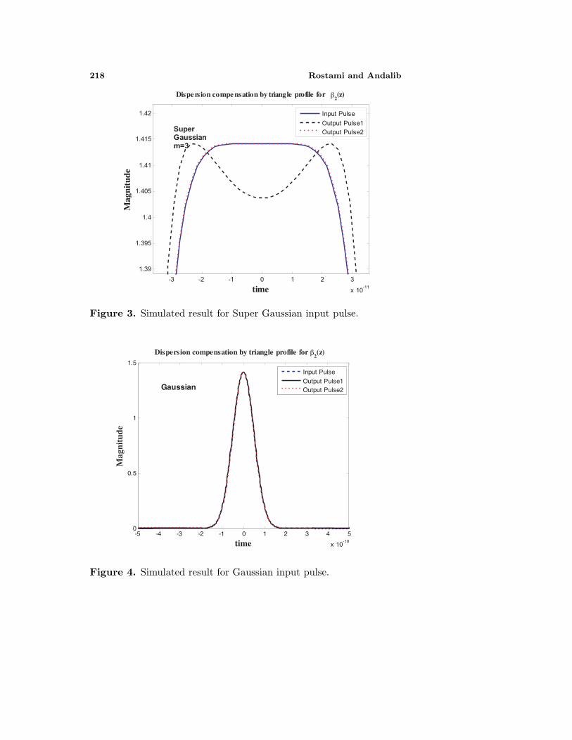
218 Rostami and Andalib
-3 -2 -1 0 1 2 3
x 10-11
1.39
1.395
1.4
1.405
1.41
1.415
1.42
Dispe rsion compe nsation by triangle profile for 2(z)
time
edutingaM
Input Pulse
Output Pulse1Output Pulse2Super
Gaussianm=3
�β
Figure 3. Simulated result for Super Gaussian input pulse.
-5 -4 -3 -2 -1 0 1 2 3 4 5
x 10-10
0
0.5
1
1.5
time
Mag
nitu
de
Input Pulse
Output Pulse1Output Pulse2Gaussian
Dispersion compensation by triangle profile for β2(z)
Figure 4. Simulated result for Gaussian input pulse.

Progress In Electromagnetics Research, PIER 75, 2007 219
-5 -4 -3 -2 -1 0 1 2 3 4 5
x 10-10
0
0.5
1
1.5
Dispersion compensation by triangle profile for �β2(z)
time
Mag
nitu
de
Input Pulse
Output Pulse1Output Pulse2Sech
Figure 5. Simulated result for Sech input pulse.
-5 -4 -3 -2 -1 0 1 2 3 4 5
x 10-10
0
0.5
1
1.5
time
edutingaM
Input Pulsewithout compensation
with compensationM. compensationSuper Gaussian
m=3
Figure 6. Simulated result for Super Gaussian input pulse.

220 Rostami and Andalib
-3 -2 -1 0 1 2 3 4
x 10-11
1.34
1.35
1.36
1.37
1.38
1.39
1.4
1.41
time
Mag
nitu
de
Input Pulsewithout compensation
with compensationM. compensation
Super Gaussianm=3
Figure 7. Simulated result for Super Gaussian input pulse.
-5 -4 -3 -2 -1 0 1 2 3 4 5
x 10-10
0
0.5
1
1.5
time
Mag
nitu
de
Input Pulsewithout compensation
with compensationM. compensationGaussian
Figure 8. Simulated result for Gaussian input pulse.

Progress In Electromagnetics Research, PIER 75, 2007 221
-5 -4 -3 -2 -1 0 1 2 3 4 5
x 10-10
0
0.5
1
1.5
time
Mag
nitu
de
Input Pulsewithout compensation
with compensationM. compensation
Sech
Figure 9. Simulated result for Super Gaussian input pulse.
with rectangular (label: with compensation) and damped triangular(label: M. compensation) GVD profiles. Also, it is observed that GVDprofile obtained from the proposed differential equation is successfulthan other profiles.
In this section some simulated results based on obtaineddifferential equations and numerical analysis of pulse propagationthrough optical fibers were presented and compared together. It wasshown that the proposed optimum differential equation for GVD is sopowerful method for compensation.
4. CONCLUSION
In this paper we have derived an integro-differential equation managingoptimum group velocity dispersion. We have simulated the proposedGVD profile and compared with traditional GVD profiles for dispersioncompensation. We have observed that the GVD profile obtained fromthe proposed differential equation is operated so better than traditionalcases. We think that the proposed method for dispersion compensationwill open a new insight in the field of dispersion compensation.

222 Rostami and Andalib
REFERENCES
1. Agrawal, G. P., Fiber Optic Communication Systems, 3rd edition,John Wiley & Sons, 2002.
2. Pandey, P. C., A. Mishra, and S. P. Ojha, “Modal dispersioncharacteristics of a single mode dielectric optical waveguide witha guiding region cross-section bounded by two involuted spirals,”Progress In Electromagnetics Research, PIER 73, 1–13, 2007.
3. Wedding, B., B. Franz, and B. Junginger, “10-Gb/s opticaltransmission up to 253 km via standard single mode fiber usingthe method of dispersion supported transmission,” Journal ofLightwave Technology, Vol. 12, 1720–1727, 1994.
4. Perlicki, K. and J. Siuzdak, “Dispersion supported transmissionwith a binary optical signal at the receiver,” Opt. QuantumElectronics, Vol. 31, 243–247, 1999.
5. Morgado, J. A. V. and A. V. T. Cartaxo, “Optimized filtering forAMI-RZ and DCS-RZ SSB signals in 40-Gb/s/ch based UDWDMsystems,” IEEE Photonics Technology Letters, Vol. 17, No. 1, 223–225, 2005.
6. Agrawal, G. P. and N. A. Olsson, “Amplification and compressionof weak picosecond optical pulses by using semiconductor-laseramplifiers,” Opt. Lett., Vol. 14, 500–502, 1989.
7. Agrawal, G. P. and N. A. Olsson, “Self-phase modulation andspectral broadening of optical pulses in semiconductor laseramplifiers,” IEEE J. Quantum Electronics, Vol. 25, 2297–2306,1989.
8. Antos, A. J. and D. K. Smith, “Design and characterizationof dispersion compensating fiber based on the LP01 mode,” J.Lightwave Technology, Vol. 12, 1739–1745, 1994.
9. Onishi, M., T. Kashiwada, Y. Ishiguro, Y. Koyano, M. Nishimura,and H. Kanamori, “High performance dispersion compensatingfibers,” Fiber Integrated Optics, Vol. 16, 277–285, 1997.
10. Liu, J., Y. L. Lam, Y. C. Chan, Y. Zhou, B. S. Ooi, G. Tan, andJ. Yao, “Embossed Bragg gratings based on organically modifiedsilane waveguides in InP,” Appl. Opt., Vol. 39, 4942–4945, 2000.
11. Gruner-Nielsen, L., S. N. Knudsen, B. Edvold, T. Veng,D. Magnussen, C. C. Larsen, and H. Damsgaard, “Dispersioncompensating fibers,” Optical Fiber Technology, Vol. 6, 164–180,2000.
12. Singh, S. P. and N. Singh, “Nonlinear effects in opticalfibers: Origin, management and applications,” Progress InElectromagnetics Research, PIER 73, 249–275, 2007.

Progress In Electromagnetics Research, PIER 75, 2007 223
13. Ibrahim, A.-B. M. A. and P. K. Choudhury, “Relative powerdistributions in omniguiding photonic band-gap fibers,” ProgressIn Electromagnetics Research, PIER 72, 269–278, 2007.
14. Biswas, A., “Dynamics of Gaussian and super-Gaussian solitonsin birefringent optical fibers,” Progress In ElectromagneticsResearch, PIER 33, 119–139, 2001.
15. Grobe, K. and H. Braunisch, “A broadband model forsingle-mode fibers including nonlinear dispersion,” Progress InElectromagnetics Research, PIER 22, 131–148, 1999.
16. Oullette, F., “Dispersion cancellation using linearly chirped Bragggrating filters in optical waveguides,” Optics Letters, Vol. 12, 847–849, 1987.
17. Pandey, P. C., A. Mishra, and S. P. Ojha, “Modal dispersioncharacteristics of a single mode dielectric optical waveguide witha guiding region cross-section bounded by two involuted spirals,”Progress In Electromagnetics Research, PIER 73, 1–13, 2007.
18. Singh, V., Y. Prajapati, and J. P. Saini, “Modal analysis anddispersion curves of a new unconventional Bragg waveguide usinga very simple method,” Progress In Electromagnetics Research,PIER 64, 191–204, 2006.
19. Yariv, A., D. Fekete, and D. M. Pepper, “Compensation forchannel dispersion by nonlinear optical phase conjugation,” OpticsLetters, Vol. 4, 52–54, 1979.
20. Kartalopoulos, S. V., DWDM Networks, Devices and Technology,IEEE, 2003.
21. Xu, B. and M. Brandt-Pearce, “Comparison of FWM and XPMinduced crosstalk using Volterra series transfer function method,”Journal of Lightwave Technology, Vol. 21, 40–53, Jan. 2003.
22. Xu, B. and M. Brandt-Pearce, “Modified Volterra series transferfunction method,” IEEE Photon. Technology Lett., 47–49, 2002.
23. Peddanarappagari, K. V. and M. Brandt-Pearce, “Volterra seriestransfer function of single-mode fibers,” Journal of LightwaveTechnology, Vol. 15, 2232–2241, Dec. 1997.
24. Peddanarappagari, K. V. and M. Brandt-Pearce, “Volterraseries approach for optimizing fiber-optic communication systemdesigns,” Journal of Lightwave Technology, Vol. 16, 2046–2055,Nov. 1998.
25. Francois, P. L., “Nonlinear propagation of ultra short pulses inoptical fibers: total field formulation in the frequency domain,”Journal of Optical Society of America, B, Vol. 8, No. 2, 276–293,February 1991.

224 Rostami and Andalib
26. Rugh, W. J., Nonlinear Systems Theory the Volterra/WienerApproach, The John Hopkins University Press, 2001.
27. Peddanarappagari, K. V., “Design and analysis of digital direct-detection fiber-optic communication systems using Volterra seriesapproach, Ph.D. Thesis, Virginia, Oct. 1997.
28. Gabitov, I. R. and S. K. Turitsyn, “Averaged pulse dynamicsin a cascaded transmission system with passive dispersioncompensation,” Optics Letters, Vol. 21, No. 5, 327–329, 1996.
29. Ablowitz, M. J. and G. Biondini, “Multiscale pulse dynamicsin communication systems with strong dispersion-management,”Optics Letters, Vol. 23, No. 21, 1668–1670, 1998.
30. Biswas, A., “Gabitov-Turitsyn equation for solitons in opticalfibers,” Journal of Nonlinear Optical Physics and Applications,Vol. 12, No. 1, 17–37, 2003.
31. Biswas, A., “Higher-order Gabitov-Turitsyn equation for solitonsin optical fibers,” Optik-International Journal for Light andElectron. Optics, Vol. 118, No. 3, 120–133, 2007.