Multi-objective Mathematical Programming Model for Optimum ...

التجارة والتمويلمجلة

https://caf.journals.ekb.eg /

جامعة طنطا –كلية التجارة

الرابع: العدد 2021ديسمبر

https://caf.journals.ekb.eg/

Multi-objective Mathematical Programming

Model for Optimum Stratification in Multivariate

Stratified Sampling

Ramadan Hamid

Professor of Statistics and Operation Research

Faculty of Economics and Political Science,

Cairo University, Egypt.

Research Professor Social

Research Center, AUC

Email: [email protected]

--------------------------------------------------------------------

Elham A. Ismail

Professor of Statistics and Operation Research

Statistics DEPT

Deen of Faculty of commerce - AL Azhar University Girl's Branch

Nasr City, Cairo, Egypt


--------------------------------------------------------------------

Safia M. Ezzat

Teaching in Statistics DEPT

Faculty of commerce - AL Azhar University Girl's Branch



--------------------------------------------------------------------

Fatma S. Abo- El.Hassan

Teaching Assistant in Statistics DEPT

Faculty of commerce - AL Azhar University Girl's Branch


Mobile: +20-10-08816160


- 191 -

Multi-objective Mathematical Programming Model for

Optimum Stratification in Multivariate Stratified Sampling

Abstract

Obtaining accurate and reliable data when conducting surveys

requires a long time, budget and large workforce so cost and time are

especially very important objectives of most surveys thus they are

necessitating to be under consideration. Most surveys are conducted in

an environment of severe budget constraints and a specific time is

required to finish the survey. The data is used to estimate the

parameters, determine the characteristics of the population under

study, and the possibility of prediction and decision-making.

The study suggested mathematical goal programming model

does not depend on a lot of data or surveys, but depends on the

distribution, parameters of any population through previous data for

the community. A multi-objective model depend on time and cost

used to evaluate the performance of the suggested mathematical goal

programming model for exponential distribution.

The suggested Mathematical goal programming model used for

getting Optimum Stratum Boundary and allocate sample size into

different strata using two auxiliary variables as stratification factors. A

numerical example is presented and the results of the suggested

mathematical goal programming are satisfying.

Key words: Multivariate Stratified Random sampling,

Optimum Stratum Boundary, Exponential distribution, Mathematical

Goal programming, Time , Cost.

- 192 -

1. Introduction

In stratified random sampling. The basic idea is that the

internally strata units should be as homogeneous as possible, that is,

stratum variances should be as small as possible.

The equations for determining the optimum stratum boundaries

was first provided by Dalenius 1950. Khan et al (2002,2005,2008

and 2009) studied the optimum strata width as a Mathematical

Programming Problem that was solved using the dynamic

programming technique. The study concerned with variables which

follows triangular, uniform, exponential, normal, right triangular,

Cauchy and power distribution. When the study variable has a pareto

frequency distribution, Rao et al.(2014) suggested a procedure

for determining optimum stratum boundary and optimum strata size

of each stratum. Fonolahi and Khan(2014) presented a solution to

evaluate the optimum strata boundaries When the measurement unit

cost varies throughout the strata, when the variable distribution is

exponentially distributed. Reddy et. al. (2016) solved the same

problem when multiple survey variables are under consideration.

Danish et al. (2017) presented optimum strata boundaries as a non-

linear programming problem when the cost per unit varies throughout

the strata. Reddy et. al. (2018) formulated the stated problem under

Neyman allocation. Where the auxiliary variables follow Weibull

distributions. Danish and Rizvi (2019) suggested a non-linear

programming model to determine optimum strata boundaries for two

- 193 -

auxiliary variables. Reddy and Khan (2020) implemented the problem

of optimum stratum boundary for various distributions using R

package.

In this study auxiliary variable(s), which can be historical data,

have also been utilized to improve the precision of study variable

estimations. When the auxiliary variable's frequency distribution is

known.

The aim of this study is to determine optimum stratum

boundary (OSB), Optimum sample size, Optimum cost and Optimum

time when two auxiliary variables used as basis for stratification.

2. Optimum Stratum Boundaries Model

Let the target population consisting of "𝑁" units be stratified

into 𝐼 strata based on 𝑝 auxiliary variables 𝑥1, 𝑥2, … . , 𝑥𝑝 and

estimation of the mean study variable is of interest.

Consider that the study variable has the regression model of the form

𝑧 = 𝜆(𝑥1, 𝑥2, … . , 𝑥𝑝) + 𝜀 (1)

Where, 𝜆(𝑥1, 𝑥2, … . , 𝑥𝑝) is a linear or (non linear function) of 𝑥𝑟

(𝑟 = 1,2, … . 𝑝) and 𝜀 is an error term such that 𝐸(𝜀\𝑥1, 𝑥2, … . , 𝑥𝑝) =

0 and 𝑣𝑎𝑟(𝜀\𝑥1, 𝑥2, … . , 𝑥𝑝) = 𝛹(𝑥1, 𝑥2, … . , 𝑥𝑝) > 0 for all 𝑥𝑟 .

For simplicity, two auxiliary variables are taken as the basis of

stratification with one study variable according to Danish and Rizvi

(2019). They divided the whole population into 𝐼 ∗ 𝐽 strata on the basis

of two auxiliary variables say 𝑦 and 𝑞 such that the number of units in

the (𝑖, 𝑗)𝑡ℎ stratum is 𝑁𝑖𝑗 . a sample of size "n" is to be drawn from the

- 194 -

whole population and suppose that the allocation of sample size to the

(𝑖, 𝑗)𝑡ℎ stratum is 𝑛𝑖𝑗 (𝑖 = 1,2, … , 𝐼; 𝑗 = 1,2, … , 𝐽).

The value of population unit in the (𝑖, 𝑗)𝑡ℎ stratum be denoted

by 𝑧𝑖𝑗𝑙 (𝑙 = 1,2, … ,𝑁𝑖𝑗) . since the study variable is denoted by 𝑧 . the

unbiased estimate of population 𝑧̅ is

𝑧�̅�𝑡 =∑ ∑ 𝑤𝑖𝑗𝑧�̅�𝑗𝐽

𝑗=1

𝐼

𝑖=1 (2)

Where 𝑤𝑖𝑗 =𝑁𝑖𝑗

𝑁 is the stratum weight for the (𝑖, 𝑗)𝑡ℎ and 𝑧�̅�𝑗 =

1

𝑛𝑖𝑗∑ 𝑧𝑖𝑗𝑙𝑛𝑖𝑗𝑙=1 , with variance is given by

𝑣𝑎𝑟(𝑧�̅�𝑡) =∑∑(1

𝑛𝑖𝑗−1

𝑁𝑖𝑗)𝑤𝑖𝑗

2𝜎𝑖𝑗𝑧2

𝑗𝑖

(3)

Where, 𝜎𝑖𝑗𝑧2 =

1

𝑁𝑖𝑗∑ (𝑧𝑖𝑗𝑙 − 𝑧�̅�𝑗)

2𝑁𝑖𝑗𝑙=1

(4)

If the finite population correction f.p.c is ignored 𝑣𝑎𝑟(�̅�𝑠𝑡) can be

expressed as 𝑣𝑎𝑟(𝑧�̅�𝑡) =

∑ ∑𝑤𝑖𝑗2𝜎𝑖𝑗𝑧

2

𝑛𝑖𝑗𝑗𝑖 (5)

Let the regression model of 𝑧 on 𝑦 and 𝑞 be given as

𝑧 = 𝜆(𝑦, 𝑞) + 𝜀 (6)

Where, 𝜆(𝑦, 𝑞) is linear or nonlinear function of 𝑦 and q, 𝜀 is error

term such that 𝐸(𝜀\𝑦, 𝑞) = 0 and 𝑣𝑎𝑟(𝜀\𝑦, 𝑞) = 𝛹(𝑦, 𝑞) > 0 ∀ 𝑦 ∈ (𝑎, 𝑏)

and 𝑞 ∈ (𝑐, 𝑑) .

Under model (6) the stratum mean 𝜇𝑖𝑗𝑧 and the stratum variance 𝜎𝑖𝑗𝑧2

can be written as

𝜇𝑖𝑗𝑧 = 𝜇𝑖𝑗𝜆 and 𝜎𝑖𝑗𝑧2 = 𝜎𝑖𝑗𝜆

2 + 𝜎𝑖𝑗𝜀2 (7)

- 195 -

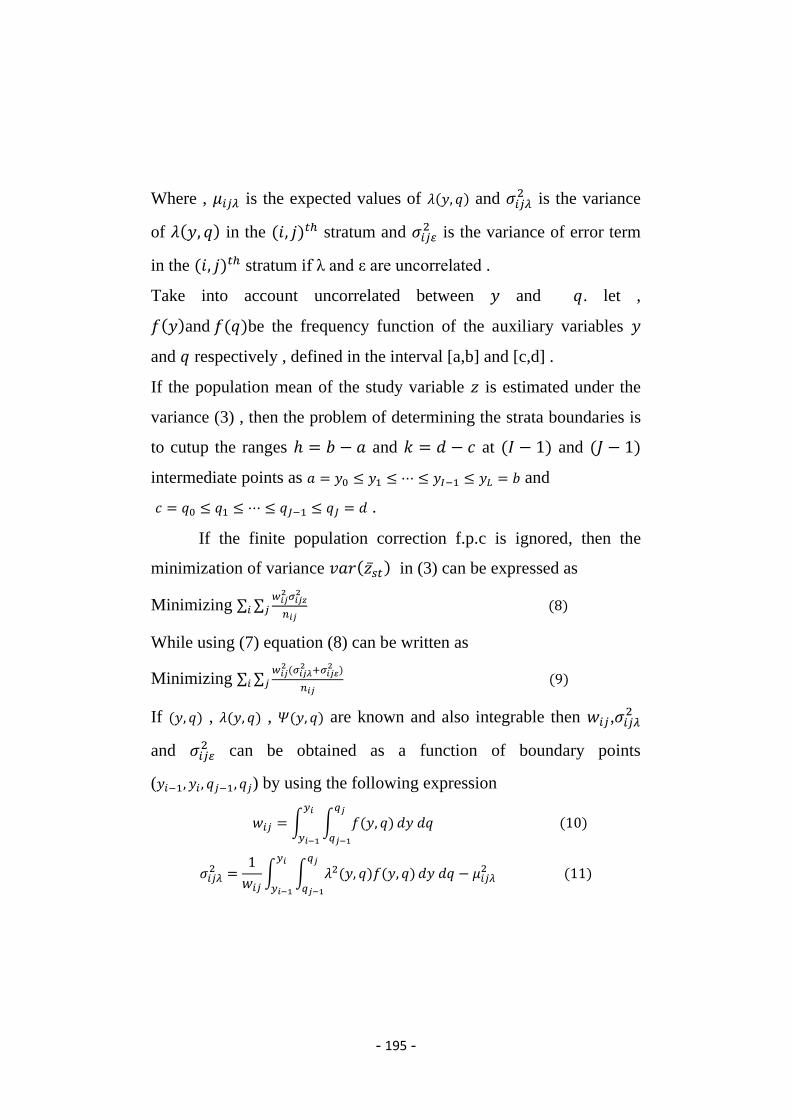
Where , 𝜇𝑖𝑗𝜆 is the expected values of 𝜆(𝑦, 𝑞) and 𝜎𝑖𝑗𝜆2 is the variance

of 𝜆(𝑦, 𝑞) in the (𝑖, 𝑗)𝑡ℎ stratum and 𝜎𝑖𝑗𝜀2 is the variance of error term

in the (𝑖, 𝑗)𝑡ℎ stratum if λ and ε are uncorrelated .

Take into account uncorrelated between 𝑦 and 𝑞. let ,

𝑓(𝑦)and 𝑓(𝑞)be the frequency function of the auxiliary variables 𝑦

and 𝑞 respectively , defined in the interval [a,b] and [c,d] .

If the population mean of the study variable 𝑧 is estimated under the

variance (3) , then the problem of determining the strata boundaries is

to cutup the ranges ℎ = 𝑏 − 𝑎 and 𝑘 = 𝑑 − 𝑐 at (𝐼 − 1) and (𝐽 − 1)

intermediate points as 𝑎 = 𝑦0 ≤ 𝑦1 ≤ ⋯ ≤ 𝑦𝐼−1 ≤ 𝑦𝐿 = 𝑏 and

𝑐 = 𝑞0 ≤ 𝑞1 ≤ ⋯ ≤ 𝑞𝐽−1 ≤ 𝑞𝐽 = 𝑑 .

If the finite population correction f.p.c is ignored, then the

minimization of variance 𝑣𝑎𝑟(𝑧�̅�𝑡) in (3) can be expressed as

Minimizing ∑ ∑𝑤𝑖𝑗2𝜎𝑖𝑗𝑧

2


While using (7) equation (8) can be written as

Minimizing ∑ ∑𝑤𝑖𝑗2 (𝜎𝑖𝑗𝜆

2 +𝜎𝑖𝑗𝜀2 )


If (𝑦, 𝑞) , 𝜆(𝑦, 𝑞) , 𝛹(𝑦, 𝑞) are known and also integrable then 𝑤𝑖𝑗,𝜎𝑖𝑗𝜆2

and 𝜎𝑖𝑗𝜀2 can be obtained as a function of boundary points

(𝑦𝑖−1, 𝑦𝑖 , 𝑞𝑗−1, 𝑞𝑗) by using the following expression

𝑤𝑖𝑗 = ∫ ∫ 𝑓(𝑦, 𝑞)𝑞𝑗

𝑞𝑗−1

𝑦𝑖

𝑦𝑖−1

𝑑𝑦 𝑑𝑞 (10)

𝜎𝑖𝑗𝜆2 =

1

𝑤𝑖𝑗∫ ∫ 𝜆2(𝑦, 𝑞)𝑓(𝑦, 𝑞)

𝑞𝑗

𝑞𝑗−1

𝑦𝑖

𝑦𝑖−1

𝑑𝑦 𝑑𝑞 − 𝜇𝑖𝑗𝜆2 (11)

- 196 -

𝜇𝑖𝑗𝜆 =1

𝑤𝑖𝑗∫ ∫ 𝜆(𝑦, 𝑞)𝑓(𝑦, 𝑞)

𝑞𝑗

𝑞𝑗−1

𝑦𝑖

𝑦𝑖−1


And (𝑦𝑖−1, 𝑦𝑖 , 𝑞𝑗−1, 𝑞𝑗) are the boundary points of the (𝑖, 𝑗)𝑡ℎ stratum.

Thus the objective function (9) could be expressed as the function of

boundary points (𝑦𝑖−1, 𝑦𝑖 , 𝑞𝑗−1, 𝑞𝑗) only . let

𝜙𝑖𝑗(𝑦𝑖−1, 𝑦𝑖 , 𝑞𝑗−1, 𝑞𝑗) =𝑤𝑖𝑗2 (𝜎𝑖𝑗𝜆

2 + 𝜎𝑖𝑗𝜀2 )

𝑛𝑖𝑗 (13)

And the ranges as

ℎ = 𝑏 − 𝑎 = 𝑦𝐼 − 𝑦0 (14)

𝑘 = 𝑑 − 𝑐 = 𝑞𝐽 − 𝑞0 (15)

Then in the bivariate stratification, a problem of determining stratum

boundary (𝑦𝑖 , 𝑞𝑗) is to break up the ranges (14),(15) at intermediate

points to estimate 𝑦1 ≤ 𝑦2 ≤ ⋯ ≤ 𝑦𝐼−2 ≤ 𝑦𝐼−1 and 𝑞1 ≤ 𝑞2 ≤ ⋯ ≤

𝑞𝐽−2 ≤ 𝑞𝐽−1 .then the problem of obtaining OSB (𝑦𝑖 , 𝑞𝑗) is to

𝑚𝑖𝑛𝑖𝑚𝑖𝑧𝑒 ∑∑𝜙𝑖𝑗(𝑦𝑖−1, 𝑦𝑖 , 𝑞𝑗−1, 𝑞𝑗)

𝑗𝑖

(16)

𝑠𝑢𝑏𝑗𝑒𝑐𝑡 𝑡𝑜 𝑎 = 𝑦0 ≤ 𝑦1 ≤ ⋯ ≤ 𝑦𝐼−1 ≤ 𝑦𝐼 = 𝑏

𝑐 = 𝑞0 ≤ 𝑞1 ≤ ⋯ ≤ 𝑞𝐽−1 ≤ 𝑞𝐽 = 𝑑

Let ℎ𝑖 = 𝑦𝑖 − 𝑦𝑖−1 and 𝑘𝑗 = 𝑞𝑗 − 𝑞𝑗−1 denote the total length or width

of (𝑖, 𝑗)𝑡ℎ stratum. With the above definition of ℎ𝑖 and 𝑘𝑗 the equation

(14) and (15) can be expressed as

∑ℎ𝑖𝑖

=∑(𝑦𝑖 − 𝑦𝑖−1)

𝑖

= 𝑏 − 𝑎 = ℎ (17)

∑𝑘𝑗𝑗

=∑(𝑞𝑗 − 𝑞𝑗−1)

𝑗

= 𝑑 − 𝑐 = 𝑘 (18)

- 197 -

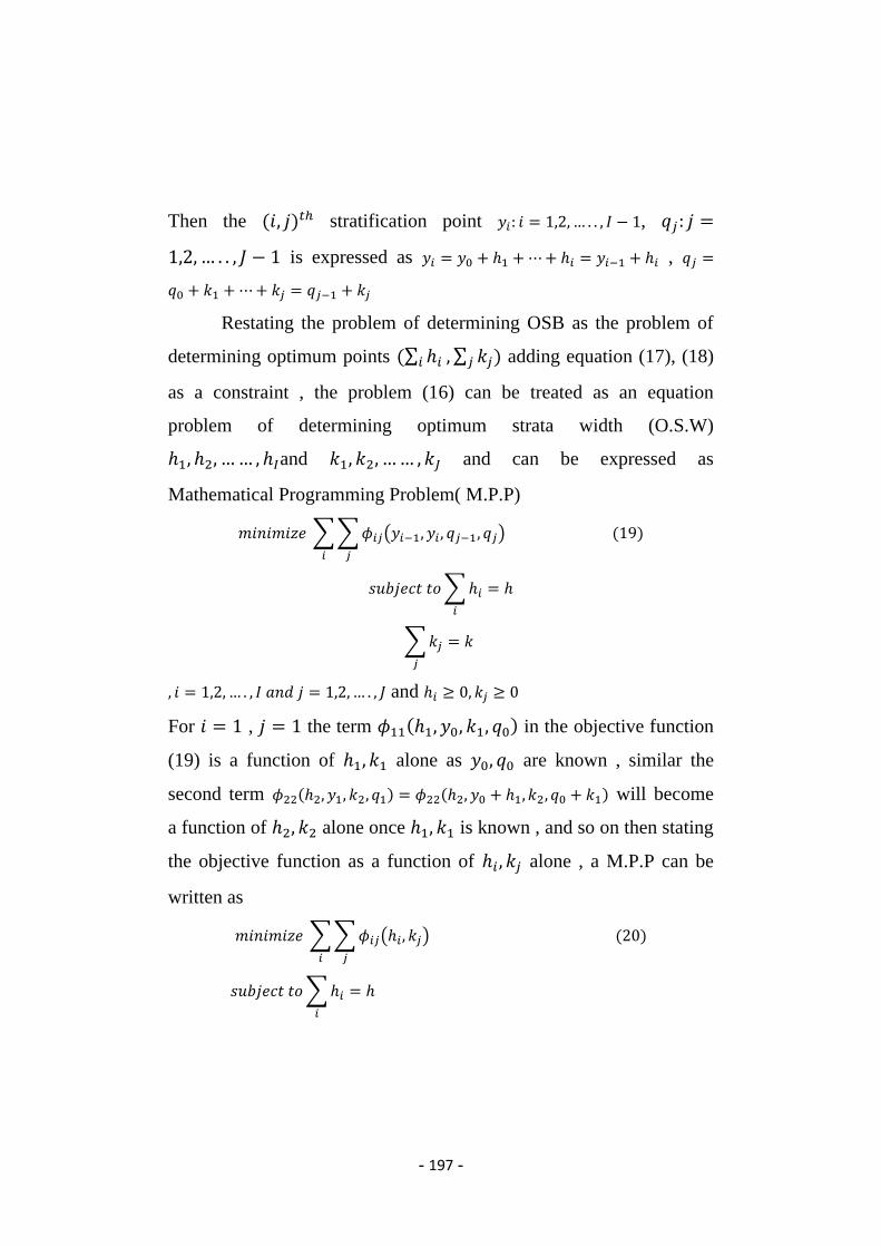
Then the (𝑖, 𝑗)𝑡ℎ stratification point 𝑦𝑖: 𝑖 = 1,2, … . . , 𝐼 − 1, 𝑞𝑗: 𝑗 =

1,2, … . . , 𝐽 − 1 is expressed as 𝑦𝑖 = 𝑦0 + ℎ1 +⋯+ ℎ𝑖 = 𝑦𝑖−1 + ℎ𝑖 , 𝑞𝑗 =

𝑞0 + 𝑘1 +⋯+ 𝑘𝑗 = 𝑞𝑗−1 + 𝑘𝑗

Restating the problem of determining OSB as the problem of

determining optimum points (∑ ℎ𝑖𝑖 , ∑ 𝑘𝑗𝑗 ) adding equation (17), (18)

as a constraint , the problem (16) can be treated as an equation

problem of determining optimum strata width (O.S.W)

ℎ1, ℎ2, …… , ℎ𝐼and 𝑘1, 𝑘2, …… , 𝑘𝐽 and can be expressed as

Mathematical Programming Problem( M.P.P)

𝑚𝑖𝑛𝑖𝑚𝑖𝑧𝑒 ∑∑𝜙𝑖𝑗(𝑦𝑖−1, 𝑦𝑖 , 𝑞𝑗−1, 𝑞𝑗)

𝑗𝑖

(19)

𝑠𝑢𝑏𝑗𝑒𝑐𝑡 𝑡𝑜∑ℎ𝑖𝑖

= ℎ

∑𝑘𝑗𝑗

= 𝑘

, 𝑖 = 1,2, … . , 𝐼 𝑎𝑛𝑑 𝑗 = 1,2,… . , 𝐽 and ℎ𝑖 ≥ 0, 𝑘𝑗 ≥ 0

For 𝑖 = 1 , 𝑗 = 1 the term 𝜙11(ℎ1, 𝑦0, 𝑘1, 𝑞0) in the objective function

(19) is a function of ℎ1, 𝑘1 alone as 𝑦0, 𝑞0 are known , similar the

second term 𝜙22(ℎ2, 𝑦1, 𝑘2, 𝑞1) = 𝜙22(ℎ2, 𝑦0 + ℎ1, 𝑘2, 𝑞0 + 𝑘1) will become

a function of ℎ2, 𝑘2 alone once ℎ1, 𝑘1 is known , and so on then stating

the objective function as a function of ℎ𝑖 , 𝑘𝑗 alone , a M.P.P can be

written as

𝑚𝑖𝑛𝑖𝑚𝑖𝑧𝑒 ∑∑𝜙𝑖𝑗(ℎ𝑖, 𝑘𝑗)

𝑗𝑖

(20)


= ℎ

- 198 -

∑𝑘𝑗𝑗

= 𝑘

, 𝑖 = 1,2, … . , 𝐼 𝑎𝑛𝑑 𝑗 = 1,2,… . , 𝐽 and ℎ𝑖 ≥ 0, 𝑘𝑗 ≥ 0

3. The Suggested Mathematical Goal Programming Model

The suggested Mathematical goal programming model for

evaluating OSB and optimum sample size allocation to the strata when

the number of strata (𝐼 ∗ 𝐽) and the total sample size (𝑛) are

predetermined ,was presented in this section.

Assume that the regression model defined in equation (6) is a linear

as:

𝑧 = 𝐴 + 𝐵𝑦 + 𝐸𝑞 + 𝑒

When the error term and two auxiliary variables are independent, we

get

𝜎𝑖𝑗𝑧2 = 𝐵2𝜎𝑖𝑗𝑦

2 + 𝐸2𝜎𝑖𝑗𝑞2 (21)

Where, 𝐵 and 𝐸 are the estimates of regression coefficients.

𝜎𝑖𝑗𝑦2 =

1

𝑤𝑖𝑗∫ ∫ 𝑦2𝑓(𝑦, 𝑞)

𝑦𝑖

𝑦𝑖−1

𝑞𝑗

𝑞𝑗−1

𝑑𝑦 𝑑𝑞 − 𝜇𝑖𝑗𝑦2 (22)

𝜎𝑖𝑗𝑞2 =

1

𝑤𝑖𝑗∫ ∫ 𝑞2𝑓(𝑦, 𝑞)

𝑞𝑗

𝑞𝑗−1

𝑦𝑖

𝑦𝑖−1

𝑑𝑦 𝑑𝑞 − 𝜇𝑖𝑗𝑞2 (23)

𝑤𝑖𝑗 = ∫ ∫ 𝑓(𝑦, 𝑞)𝑞𝑗

𝑞𝑗−1

𝑦𝑖

𝑦𝑖−1


𝜇𝑖𝑗𝑦 =1

𝑤𝑖𝑗∫ ∫ 𝑦𝑓(𝑦, 𝑞)

𝑦𝑖

𝑦𝑖−1

𝑞𝑗

𝑞𝑗−1


𝜇𝑖𝑗𝑞 =1

𝑤𝑖𝑗∫ ∫ 𝑞𝑓(𝑦, 𝑞)

𝑞𝑗

𝑞𝑗−1

𝑦𝑖

𝑦𝑖−1


- 199 -

To optimally determine stratum boundaries and allocate the sample to

the different strata under multi-objective model.

Applying the variance formula in (8) and substituting in (21).Thus the

model can be formulated as:

𝑚𝑖𝑛𝑖𝑚𝑖𝑧𝑒 ∑∑𝑤𝑖𝑗2 (𝐵2𝜎𝑖𝑗𝑦

2 + 𝐸2𝜎𝑖𝑗𝑞2 )

𝑛𝑖𝑗𝑗𝑖

(27)


= ℎ

,∑𝑘𝑗𝑗

= 𝑘

∑∑𝑛𝑖𝑗 = 𝑛

𝑗𝑖

, 𝑖 = 1,2, … . , 𝐼 𝑎𝑛𝑑 𝑗 = 1,2,… . , 𝐽 , 1 ≤ 𝑛𝑖𝑗 ≤ 𝑁𝑖𝑗

and ℎ𝑖 ≥ 0, 𝑘𝑗 ≥ 0

The suggested mathematical goal programming constraints are

as follows:

1- The aggregate of the optimum stratum width be equal to the

distribution's range.

2- The cost (not exceed a fixed limit according to budget of

survey) was added to the model as objective constrain need

to minimize.

3- The time is another important constraint which needed for

the sampling process within a specific range.

Then the suggested Goal programming approach can be formulated

as:

Minimize 𝑑𝑝1 + 𝑑𝑛1 + 𝑑𝑝2 + 𝑑𝑛2 + 𝑑𝑝3 + 𝑑𝑛3 (28)

- 200 -

Subject to

∑∑𝑤𝑖𝑗2 (𝐵2𝜎𝑖𝑗𝑦

2 + 𝐸2𝜎𝑖𝑗𝑞2 )


+ 𝑑𝑛1 − 𝑑𝑝1 = 𝑣 (29)

∑∑𝑐𝑖𝑗𝑗𝑖

𝑛𝑖𝑗 + 𝑑𝑛2 − 𝑑𝑝2 = 𝐶 (30)

∑∑𝑡𝑖𝑗𝑗𝑖

𝑛𝑖𝑗 + 𝑑𝑛3 − 𝑑𝑝3 = 𝑇 (31)

∑ ℎ𝑖𝐼

𝑖=1= ℎ (32)

𝑦𝑖 = 𝑦𝑖−1 + ℎ𝑖 (33)

∑ 𝑘𝑗𝐽

𝑗=1= 𝑘 (34)

𝑞𝑗 = 𝑞𝑗−1 + 𝑘𝑗 (35)

∑∑𝑛𝑖𝑗𝑗𝑖

= 𝑛 𝑖 = 1,2, … , 𝐼 , 𝑗 = 1,2, … , 𝐽 (36)

ℎ𝑖 ≥ 0, 𝑘𝑗 ≥ 0 , 1 ≤ 𝑛𝑖𝑗 ≤ 𝑁𝑖𝑗 , 𝑑𝑝1,𝑑𝑝2,𝑑𝑝3, 𝑑𝑛1, 𝑑𝑛2,𝑑𝑛3 ≥ 0

Where ,

𝑛𝑖𝑗: Sample size of the 𝑖𝑗th stratum

𝑛 = ∑ ∑ 𝑛𝑖𝑗𝑗𝑖 : Total sample size

𝑐𝑖𝑗: per unit cost of the 𝑖𝑗th stratum

𝐶: total cost

𝑡𝑖𝑗: time per unit of the 𝑖𝑗th stratum

𝑇 total time

𝑣 prefixed variance of the estimator of the population mean

𝑑𝑝1,𝑑𝑝2,𝑑𝑝3, 𝑑𝑛1, 𝑑𝑛2,𝑑𝑛3 are positive and negative deviation variables

of goals where first goal is to minimize 𝑉( 𝑧�̅�𝑡) , second and third

- 201 -

goals are to minimize cost and time of collecting data per unit in each

stratum respectively, 𝑤𝑖𝑗2 (𝐵2𝜎𝑖𝑗𝑦

2 +𝐸2𝜎𝑖𝑗𝑞2 )

𝑛𝑖𝑗= 𝑉( 𝑧�̅�𝑡) if the finite population

correction is ignored, 𝑁𝑖𝑗: Stratum size of the 𝑖𝑗th stratum.

4. Numerical example

This section concerned with the numerical example for the

suggested Mathematical goal programming model, the numerical

example take the following step:-

1. Because of its simple mathematical form the study chosen the

two auxiliary variables which chosen followed exponential

distribution as an application of the idea of a multi-objective

model for obtaining optimum stratum boundary and allocation

the sample into different strata with pdf as:

𝑓(𝑦) = {𝜃𝑒−𝜃𝑦 , 𝑦 ≥ 0

0 𝑜𝑡ℎ𝑒𝑟𝑤𝑖𝑠𝑒 (37)

, 𝑓(𝑞) = {𝜆𝑒−𝜆𝑞 , 𝑞 ≥ 0

0 𝑜𝑡ℎ𝑒𝑟𝑤𝑖𝑠𝑒 (38)

By using (22), (23),(24) and (37),(38) the term 𝑊𝑖𝑗 , 𝜎𝑖𝑗𝑦2 and 𝜎𝑖𝑗𝑞

2 can

be expressed as

𝑊𝑖𝑗 = 𝑒−𝜃𝑦𝑖𝑒−𝜆𝑞𝑗(𝑒𝜃ℎ𝑖 − 1)(𝑒𝜆𝑘𝑗 − 1) (39)

𝜎𝑖𝑗𝑦2 =

1𝜃2(𝑒𝜃ℎ𝑖 − 1)

2− ℎ𝑖

2𝑒𝜃ℎ𝑖

(𝑒𝜃ℎ𝑖 − 1)2 (40)

𝜎𝑖𝑗𝑞2 =

1𝜆2(𝑒𝜆𝑘𝑗 − 1)

2− 𝑘𝑗

2𝑒𝜆𝑘𝑗

(𝑒𝜆𝑘𝑗 − 1)2 (41)

- 202 -

2. To determine the OSB and optimum allocation into sample strata

which result in minimum possible variance of the estimator let 𝑦

and 𝑞 followed exponential distribution.

3. Where 𝜃 and 𝜆 are the chosen exponential distribution parameters

and (𝑦0,𝑦𝐼), (𝑞0, 𝑞𝐽) are the chosen observation of smallest and

largest values of stratification variables 𝑦 and 𝑞 respectively. ℎ

and 𝑘 are the different between largest and smallest .

4. To evaluate the performance for the suggested model , some

parameters were randomly selected for two auxiliary variables 𝑦

and 𝑞 chosen from some published researches in the field of study

have 𝜃 = .08 and 𝜆 = .05 respectively as distribution parameters

when sample size 𝑛 = 100 and 𝑦0 = 1.5 , 𝑦𝐼 = 21.5 and ℎ = 20 , 𝑞0 =

1 , 𝑞𝐽 = 16 and 𝑘 = 15.

5. The study applied the suggested model to calculate the variance

when the initial value of variance 𝑣 = 13.6 (which calculated

using Khan and Sharama (2015)), the fixed value of cost

=12000, the specific rang of time =1500 were chosen arbitrary

and the coefficients of regression are 𝐵 = .3 and 𝐸 = .7 the

values of regression coefficients were chosen for the variation

in the variables.

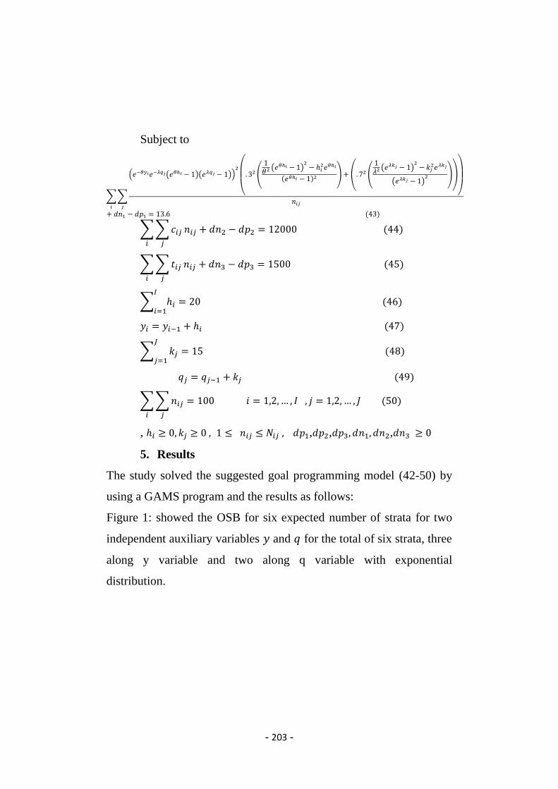
The suggested goal programming model (28-36) when the auxiliary

variables 𝑦 and 𝑞 is given by (38) by Using (39), (40) and (41), can be

formulated as:

Minimize 𝑑𝑝1 + 𝑑𝑛1 + 𝑑𝑝2 + 𝑑𝑛2 + 𝑑𝑝3 + 𝑑𝑛3 (42)

- 203 -

Subject to

∑∑

(𝑒−𝜃𝑦𝑖𝑒−𝜆𝑞𝑗(𝑒𝜃ℎ𝑖 − 1)(𝑒𝜆𝑞𝑗 − 1))2

(

.32(

1𝜃2(𝑒𝜃ℎ𝑖 − 1)

2− ℎ𝑖

2𝑒𝜃ℎ𝑖

(𝑒𝜃ℎ𝑖 − 1)2)+ (. 72 (

1𝜆2(𝑒𝜆𝑘𝑗 − 1)

2− 𝑘𝑗

2𝑒𝜆𝑘𝑗

(𝑒𝜆𝑘𝑗 − 1)2 ))

)


+ 𝑑𝑛1 − 𝑑𝑝1 = 13.6 (43)

∑∑𝑐𝑖𝑗𝑗𝑖

𝑛𝑖𝑗 + 𝑑𝑛2 − 𝑑𝑝2 = 12000 (44)

∑∑𝑡𝑖𝑗𝑗𝑖

𝑛𝑖𝑗 + 𝑑𝑛3 − 𝑑𝑝3 = 1500 (45)

∑ ℎ𝑖𝐼

𝑖=1= 20 (46)

𝑦𝑖 = 𝑦𝑖−1 + ℎ𝑖 (47)

∑ 𝑘𝑗𝐽

𝑗=1= 15 (48)

𝑞𝑗 = 𝑞𝑗−1 + 𝑘𝑗 (49)

∑∑𝑛𝑖𝑗𝑗𝑖

= 100 𝑖 = 1,2,… , 𝐼 , 𝑗 = 1,2, … , 𝐽 (50)

, ℎ𝑖 ≥ 0, 𝑘𝑗 ≥ 0 , 1 ≤ 𝑛𝑖𝑗 ≤ 𝑁𝑖𝑗 , 𝑑𝑝1,𝑑𝑝2,𝑑𝑝3, 𝑑𝑛1, 𝑑𝑛2,𝑑𝑛3 ≥ 0

5. Results

The study solved the suggested goal programming model (42-50) by

using a GAMS program and the results as follows:

Figure 1: showed the OSB for six expected number of strata for two

independent auxiliary variables 𝑦 and 𝑞 for the total of six strata, three

along y variable and two along q variable with exponential

distribution.

- 204 -

21.500

𝑦 13.559

7.038

8.500 16.000

𝑞

Table 1: The OSB Results for six expected number of strata for two

independent auxiliary variables 𝑦 and 𝑞 with exponential distribution.

OSW OSB Sample Size

(𝒏𝒊𝒋)

𝑪𝐢𝐣 𝑻𝐢𝐣 Objective

function

(05.538,7.5) (07.038,8.5) 18.14≈18 2410 296 .081

(6.521,7.5) (13.559,8.5) 18.2≈18 2428 296

(7.941,7.5) (21.500,8.5) 18.3≈19 2459 296

(05.538,7.5) (07.038,16) 15.04≈15 900 150.75

(6.521,7.5) (13.559,16) 15.09≈15 1866 150.75

(7.941,7.5) (21.500,16) 15.18≈ 𝟏𝟓 1875 277.5

The suggested Mathematical goal programming model for

determining OSB and optimum allocation of sample size to the strata

results showed in table (1)are:

1. The suggested Mathematical goal programming model

calculate the optimum stratum width and optimum stratum

boundary in satisfactory way where the new minimum value

of variance is .081 which are less than the initial value 𝑣 =

13.6 which calculated before

2. Sample size is divided in satisfactory way according to the

number of strata where the suggested model determine the size

- 205 -

of strata (𝑛1 = 18 , … 𝑛4 = 15) at the range of the total sample

size (𝑛 = 100).

3. The suggested model divided the time and cost and reducing

them as much as possible where the model was not outside the

permitted range of the proposed cost-time values.

4. As a result, we can infer that employing a single study variable

with two auxiliary variables while taking cost and time into

account And that's an extension the exciting technique with

Khan and Sharama (2015).

6. Conclusion

The study suggested Mathematical goal programming model to

determine the optimum strata boundary by bi-variate variables in

multi-objective problem with minimum variance.

1. The new minimum value of variance .081 which is less

than the initial value (𝑣 = 13.6) which chosen before

2. The cost and the time (not exceed a fixed limit

according to budget and time of survey) was added to

the model as objective constrain need to minimize.

3. The suggested mathematical goal programming help

researcher or any statistician to predict Optimum

Stratum Boundary through the available information

represented by the parameters of the appropriate

distribution that fit the nature of the data.

- 206 -

References

1. Danish, F., Rizvi, S.E.H., Jeelani, M.I. and Reashi, J.A.

(2017)"Obtaining strata boundaries under proportional

allocation with varying cost of every unit". Pakistan Journal of

Statistics and Operation Research, 13(3), 567-574.

2. Danish, F., and Rizvi, S.E.H (2019)" Optimum Stratification

by Two Stratifiction Variables Using Mathematical

Programming" Pakistan Journal of Statistics Vol. 35(1), 11-24.

3. Fanolahi, A.V. and Khan, M.G.M. (2014)" Determing the

optimum strata boundaries with constant cost factor".

Conference: IEEE Asia-Pacific World Congress on Computer

Science and Engineering (APWC), At Plantation Island, Fij.

4. Khan, E.A., Khan, M.G.M. and Ahsan, M.J. (2002). "Optimum

stratification: A mathematical programming approach".

Culcutta Statistical Association Bulletin, 52 (special), 205-208.

5. Khan, M.G.M., Sehar, N. , and Ahsan, M.J. (2005). "Optimum

stratification for exponential study variable under Neyman

allocation". Journal of Indian Society of Agricultural Statistics,

59(2), 146-150.

6. Khan, M. G. M., Nand, N., and Ahmad, N. (2008).

"Determining the optimum strata boundary points using

dynamic programming". Survey Methodology, 34(2), 205-214.

7. Khan, M. G. M., Ahmad, N. and Khan, S. (2009)."Determining

the optimum stratum boundaries using mathematical

- 207 -

programming". J. Math. Model. Algorithms, Springer,

Netherland, 8(4): 409- 423.

8. Khan, M.G.M. and Sharma, S. (2015). “Determining Optimum

Strata Boundaries and Optimum Allocation in Stratified

Sampling”, Aligarh Journal of Statistics, Vol. 35, 23-40.

9. Rao, D.K. , Khan, M.G.M. and Reddy, K.G. (2014)."Optimum

stratification of a skewed population". International journal of

mathematical, computational, natural and physical engineering,

8(3):497-500.

10. Reddy, K. G., Khan, M. G. and D. Rao (2016). "A procedure

for computing optimal stratum boundaries and sample sizes for

multivariate surveys". JSW 11(8), 816–832.

11. Reddy K.G., Khan M.G.M., Khan S. (2018) "Optimum strata

boundaries and sample sizes in health surveys using auxiliary

variables". PLoS ONE 13(4): e0194787.

12. Reddy KG and Khan MGM (2020)" stratifyR: An R Package

for optimal stratification and sample allocation for univariate

populations " Australian & New Zealand Journal of Statistics

62 (3), 383-405.

javascript:void(0)

javascript:void(0)

javascript:void(0)

Multi-objective Mathematical Programming Model for Optimum ...

Documents

Transcript of Multi-objective Mathematical Programming Model for Optimum ...