Quantitative mapping and predictive modelling of Mn-nodules ...
Upload
khangminh22Category
view
0download
0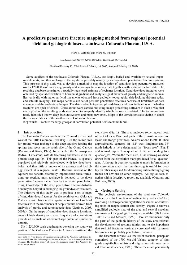
Earth Planets Space, 57, 701–715, 2005
A predictive penetrative fracture mapping method from regional potentialfield and geologic datasets, southwest Colorado Plateau, U.S.A.
Mark E. Gettings and Mark W. Bultman
U.S. Geological Survey, 520 N. Park Ave., Tucson, AZ 85719, USA
(Received February 13, 2004; Revised February 14, 2005; Accepted February 15, 2005)
Some aquifers of the southwest Colorado Plateau, U.S.A., are deeply buried and overlain by several imper-meable units, and thus recharge to the aquifer is probably mainly by seepage down penetrative fracture systems.This purpose of this study was to develop a method to map the location of candidate deep penetrative fracturesover a 120,000 km2 area using gravity and aeromagnetic anomaly data together with surficial fracture data. Theresulting database constitutes a spatially registered estimate of recharge location. Candidate deep fractures wereobtained by spatial correlation of horizontal gradient and analytic signal maxima of gravity and magnetic anoma-lies vertically with major surficial lineaments obtained from geologic, topographic, side-looking airborne radar,and satellite imagery. The maps define a sub-set of possible penetrative fractures because of limitations of datacoverage and the analysis technique. The data and techniques employed do not yield any indication as to whetherfractures are open or closed. Correlations were carried out using image processing software in such a way thatevery pixel on the resulting grids was coded to uniquely identify which datasets correlated. The technique cor-rectly identified known deep fracture systems and many new ones. Maps of the correlations also define in detailthe tectonic fabrics of the southwestern Colorado Plateau.Key words: Fracture recharge geospatial correlation potential fields tectonic fabric.
1. IntroductionThe Colorado Plateau south of the Colorado River and
west of the Little Colorado River (Fig. 1) is the source areafor ground water recharge to the deep aquifers feeding thesprings and seeps on the south side of the Grand Canyon(Robson and Banta, 1995). In particular, the MississippianRedwall Limestone, with its fracturing and karsts, is an im-portant deep aquifer. This part of the Plateau is sparselypopulated and relatively undeveloped with few deep bore-holes, and thus little is known of its geology and hydrol-ogy except at a regional scale. Because several of theaquifers are beneath essentially impermeable shale forma-tions up section, most recharge is believed to be downpenetrative fractures rather than by interstratal percolation.Thus, knowledge of the deep penetrative fracture distribu-tion may be helpful in managing the groundwater resources.The objective of this study was to produce a set of mapsof candidate deep fractures for the southwestern ColoradoPlateau derived from vertical spatial correlation of surficialfractures with the lineaments of deep structure derived fromanalysis of gravity and aeromagnetic data (Gettings, 2003,2003a). On the maps of candidate deep fracture locations,areas of high density or spatial frequency of correlationsprovide an estimate of where recharge potential is more fa-vorable.
Six 1:250,000-scale quadrangles covering the southwestportion of the Colorado Plateau in Arizona constituted the
Copyright c© The Society of Geomagnetism and Earth, Planetary and Space Sci-ences (SGEPSS); The Seismological Society of Japan; The Volcanological Societyof Japan; The Geodetic Society of Japan; The Japanese Society for Planetary Sci-ences; TERRAPUB.
study area (Fig. 1). The area includes some regions northof the Colorado River and parts of the Transition Zone andBasin and Range provinces. An area of one 1:250,000 sheetapproximately centered on 112◦ west longitude and 36◦
north latitude is here designated the “focus area” (Fig. 1)and is made up of four quarters of the surrounding fourquadrangles. Within the focus area, a line drawing was handdrawn from the correlation maps produced for all quadran-gles. Although it does not contain as much information asthe correlation maps, the line drawing is useful for over-lay on other maps and for delineating subtle through-goingtrends not obvious on other displays. All digital data, to-gether with a descriptive report are available (Gettings andBultman, 2005).
2. Geologic SettingThe geologic environment of the southwest Colorado
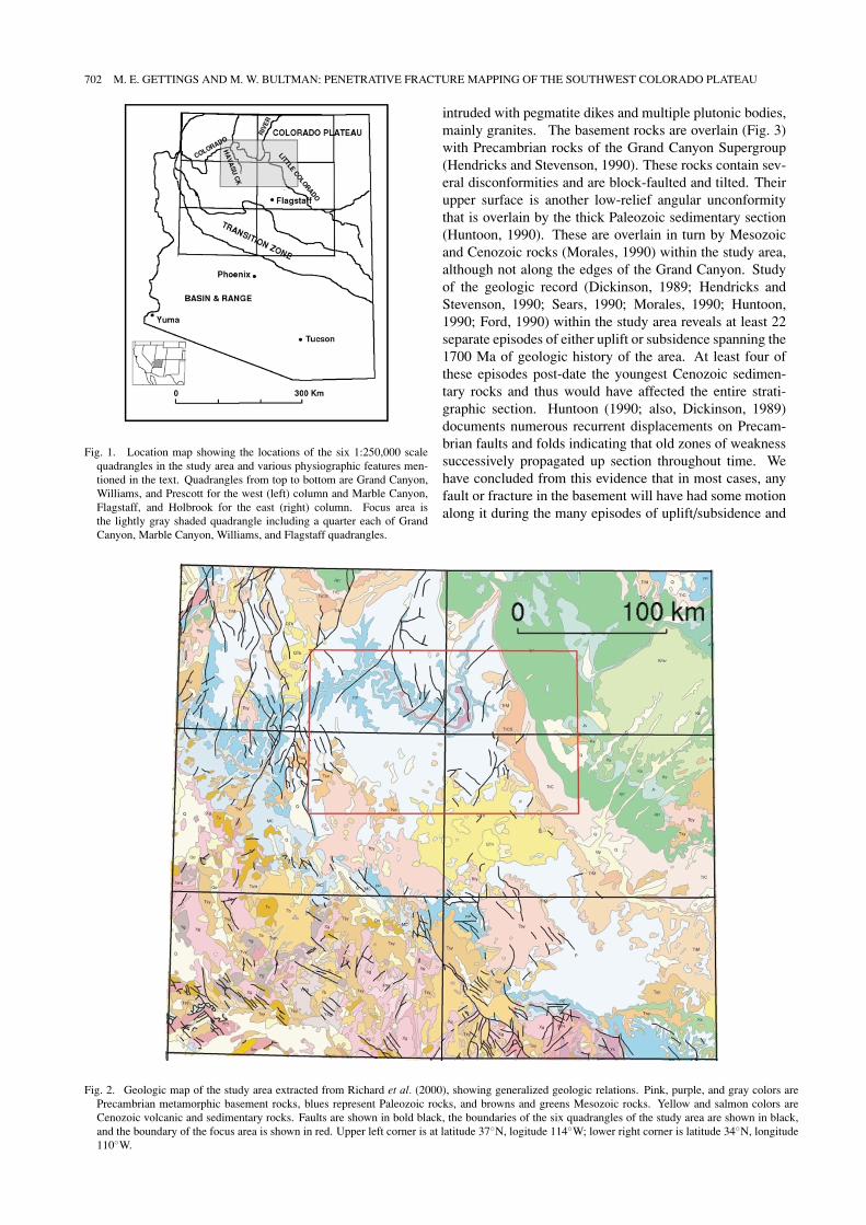
Plateau is a thick section of sedimentary rocks (1–3 km)overlying a heterogeneous crystalline basement of contrast-ing units of magnetization and density. Figure 2 shows asimplified geologic map of the area and several excellentsummaries of the geologic history are available (Dickinson,1989; Beus and Morales, 1990). Here we summarize onlythe parts of the geologic history of the study area relevantthe development of tectonic fabrics and to the hypothesisthat surficial fractures vertically correlated with basementlineaments are probably penetrative fractures.
The basement surface is a low-relief erosional peneplaincomprised of the 1700 Ma-old Vishnu complex of highgrade amphibolitic schists and migmatites with near verti-cal foliation (Babcock, 1990). These rocks are pervasively
701
702 M. E. GETTINGS AND M. W. BULTMAN: PENETRATIVE FRACTURE MAPPING OF THE SOUTHWEST COLORADO PLATEAU
Fig. 1. Location map showing the locations of the six 1:250,000 scalequadrangles in the study area and various physiographic features men-tioned in the text. Quadrangles from top to bottom are Grand Canyon,Williams, and Prescott for the west (left) column and Marble Canyon,Flagstaff, and Holbrook for the east (right) column. Focus area isthe lightly gray shaded quadrangle including a quarter each of GrandCanyon, Marble Canyon, Williams, and Flagstaff quadrangles.
Fig. 2. Geologic map of the study area extracted from Richard et al. (2000), showing generalized geologic relations. Pink, purple, and gray colors arePrecambrian metamorphic basement rocks, blues represent Paleozoic rocks, and browns and greens Mesozoic rocks. Yellow and salmon colors areCenozoic volcanic and sedimentary rocks. Faults are shown in bold black, the boundaries of the six quadrangles of the study area are shown in black,and the boundary of the focus area is shown in red. Upper left corner is at latitude 37◦N, logitude 114◦W; lower right corner is latitude 34◦N, longitude110◦W.
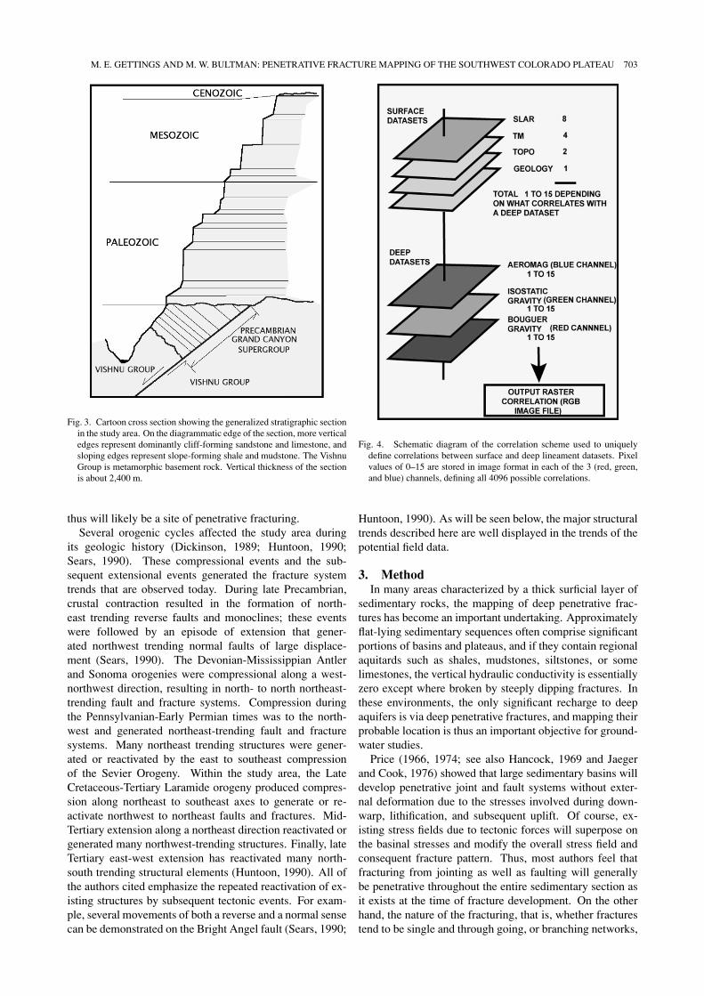
intruded with pegmatite dikes and multiple plutonic bodies,mainly granites. The basement rocks are overlain (Fig. 3)with Precambrian rocks of the Grand Canyon Supergroup(Hendricks and Stevenson, 1990). These rocks contain sev-eral disconformities and are block-faulted and tilted. Theirupper surface is another low-relief angular unconformitythat is overlain by the thick Paleozoic sedimentary section(Huntoon, 1990). These are overlain in turn by Mesozoicand Cenozoic rocks (Morales, 1990) within the study area,although not along the edges of the Grand Canyon. Studyof the geologic record (Dickinson, 1989; Hendricks andStevenson, 1990; Sears, 1990; Morales, 1990; Huntoon,1990; Ford, 1990) within the study area reveals at least 22separate episodes of either uplift or subsidence spanning the1700 Ma of geologic history of the area. At least four ofthese episodes post-date the youngest Cenozoic sedimen-tary rocks and thus would have affected the entire strati-graphic section. Huntoon (1990; also, Dickinson, 1989)documents numerous recurrent displacements on Precam-brian faults and folds indicating that old zones of weaknesssuccessively propagated up section throughout time. Wehave concluded from this evidence that in most cases, anyfault or fracture in the basement will have had some motionalong it during the many episodes of uplift/subsidence and
M. E. GETTINGS AND M. W. BULTMAN: PENETRATIVE FRACTURE MAPPING OF THE SOUTHWEST COLORADO PLATEAU 703
Fig. 3. Cartoon cross section showing the generalized stratigraphic sectionin the study area. On the diagrammatic edge of the section, more verticaledges represent dominantly cliff-forming sandstone and limestone, andsloping edges represent slope-forming shale and mudstone. The VishnuGroup is metamorphic basement rock. Vertical thickness of the sectionis about 2,400 m.
thus will likely be a site of penetrative fracturing.Several orogenic cycles affected the study area during
its geologic history (Dickinson, 1989; Huntoon, 1990;Sears, 1990). These compressional events and the sub-sequent extensional events generated the fracture systemtrends that are observed today. During late Precambrian,crustal contraction resulted in the formation of north-east trending reverse faults and monoclines; these eventswere followed by an episode of extension that gener-ated northwest trending normal faults of large displace-ment (Sears, 1990). The Devonian-Mississippian Antlerand Sonoma orogenies were compressional along a west-northwest direction, resulting in north- to north northeast-trending fault and fracture systems. Compression duringthe Pennsylvanian-Early Permian times was to the north-west and generated northeast-trending fault and fracturesystems. Many northeast trending structures were gener-ated or reactivated by the east to southeast compressionof the Sevier Orogeny. Within the study area, the LateCretaceous-Tertiary Laramide orogeny produced compres-sion along northeast to southeast axes to generate or re-activate northwest to northeast faults and fractures. Mid-Tertiary extension along a northeast direction reactivated orgenerated many northwest-trending structures. Finally, lateTertiary east-west extension has reactivated many north-south trending structural elements (Huntoon, 1990). All ofthe authors cited emphasize the repeated reactivation of ex-isting structures by subsequent tectonic events. For exam-ple, several movements of both a reverse and a normal sensecan be demonstrated on the Bright Angel fault (Sears, 1990;
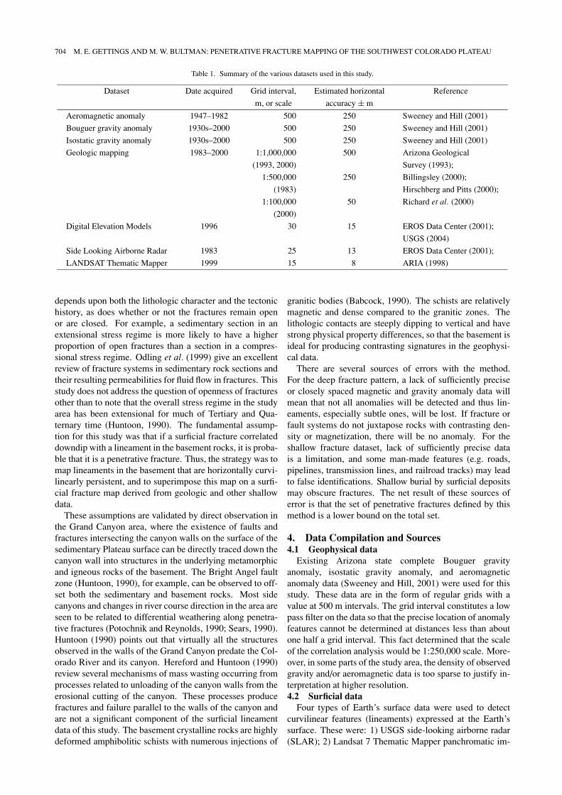
Fig. 4. Schematic diagram of the correlation scheme used to uniquelydefine correlations between surface and deep lineament datasets. Pixelvalues of 0–15 are stored in image format in each of the 3 (red, green,and blue) channels, defining all 4096 possible correlations.
Huntoon, 1990). As will be seen below, the major structuraltrends described here are well displayed in the trends of thepotential field data.
3. MethodIn many areas characterized by a thick surficial layer of
sedimentary rocks, the mapping of deep penetrative frac-tures has become an important undertaking. Approximatelyflat-lying sedimentary sequences often comprise significantportions of basins and plateaus, and if they contain regionalaquitards such as shales, mudstones, siltstones, or somelimestones, the vertical hydraulic conductivity is essentiallyzero except where broken by steeply dipping fractures. Inthese environments, the only significant recharge to deepaquifers is via deep penetrative fractures, and mapping theirprobable location is thus an important objective for ground-water studies.
Price (1966, 1974; see also Hancock, 1969 and Jaegerand Cook, 1976) showed that large sedimentary basins willdevelop penetrative joint and fault systems without exter-nal deformation due to the stresses involved during down-warp, lithification, and subsequent uplift. Of course, ex-isting stress fields due to tectonic forces will superpose onthe basinal stresses and modify the overall stress field andconsequent fracture pattern. Thus, most authors feel thatfracturing from jointing as well as faulting will generallybe penetrative throughout the entire sedimentary section asit exists at the time of fracture development. On the otherhand, the nature of the fracturing, that is, whether fracturestend to be single and through going, or branching networks,
704 M. E. GETTINGS AND M. W. BULTMAN: PENETRATIVE FRACTURE MAPPING OF THE SOUTHWEST COLORADO PLATEAU
Table 1. Summary of the various datasets used in this study.
Dataset Date acquired Grid interval, Estimated horizontal Reference
m, or scale accuracy ± m
Aeromagnetic anomaly 1947–1982 500 250 Sweeney and Hill (2001)
Bouguer gravity anomaly 1930s–2000 500 250 Sweeney and Hill (2001)
Isostatic gravity anomaly 1930s–2000 500 250 Sweeney and Hill (2001)
Geologic mapping 1983–2000 1:1,000,000 500 Arizona Geological
(1993, 2000) Survey (1993);
1:500,000 250 Billingsley (2000);
(1983) Hirschberg and Pitts (2000);
1:100,000 50 Richard et al. (2000)
(2000)
Digital Elevation Models 1996 30 15 EROS Data Center (2001);
USGS (2004)
Side Looking Airborne Radar 1983 25 13 EROS Data Center (2001);
LANDSAT Thematic Mapper 1999 15 8 ARIA (1998)
depends upon both the lithologic character and the tectonichistory, as does whether or not the fractures remain openor are closed. For example, a sedimentary section in anextensional stress regime is more likely to have a higherproportion of open fractures than a section in a compres-sional stress regime. Odling et al. (1999) give an excellentreview of fracture systems in sedimentary rock sections andtheir resulting permeabilities for fluid flow in fractures. Thisstudy does not address the question of openness of fracturesother than to note that the overall stress regime in the studyarea has been extensional for much of Tertiary and Qua-ternary time (Huntoon, 1990). The fundamental assump-tion for this study was that if a surficial fracture correlateddowndip with a lineament in the basement rocks, it is proba-ble that it is a penetrative fracture. Thus, the strategy was tomap lineaments in the basement that are horizontally curvi-linearly persistent, and to superimpose this map on a surfi-cial fracture map derived from geologic and other shallowdata.
These assumptions are validated by direct observation inthe Grand Canyon area, where the existence of faults andfractures intersecting the canyon walls on the surface of thesedimentary Plateau surface can be directly traced down thecanyon wall into structures in the underlying metamorphicand igneous rocks of the basement. The Bright Angel faultzone (Huntoon, 1990), for example, can be observed to off-set both the sedimentary and basement rocks. Most sidecanyons and changes in river course direction in the area areseen to be related to differential weathering along penetra-tive fractures (Potochnik and Reynolds, 1990; Sears, 1990).Huntoon (1990) points out that virtually all the structuresobserved in the walls of the Grand Canyon predate the Col-orado River and its canyon. Hereford and Huntoon (1990)review several mechanisms of mass wasting occurring fromprocesses related to unloading of the canyon walls from theerosional cutting of the canyon. These processes producefractures and failure parallel to the walls of the canyon andare not a significant component of the surficial lineamentdata of this study. The basement crystalline rocks are highlydeformed amphibolitic schists with numerous injections of
granitic bodies (Babcock, 1990). The schists are relativelymagnetic and dense compared to the granitic zones. Thelithologic contacts are steeply dipping to vertical and havestrong physical property differences, so that the basement isideal for producing contrasting signatures in the geophysi-cal data.
There are several sources of errors with the method.For the deep fracture pattern, a lack of sufficiently preciseor closely spaced magnetic and gravity anomaly data willmean that not all anomalies will be detected and thus lin-eaments, especially subtle ones, will be lost. If fracture orfault systems do not juxtapose rocks with contrasting den-sity or magnetization, there will be no anomaly. For theshallow fracture dataset, lack of sufficiently precise datais a limitation, and some man-made features (e.g. roads,pipelines, transmission lines, and railroad tracks) may leadto false identifications. Shallow burial by surficial depositsmay obscure fractures. The net result of these sources oferror is that the set of penetrative fractures defined by thismethod is a lower bound on the total set.
4. Data Compilation and Sources4.1 Geophysical data
Existing Arizona state complete Bouguer gravityanomaly, isostatic gravity anomaly, and aeromagneticanomaly data (Sweeney and Hill, 2001) were used for thisstudy. These data are in the form of regular grids with avalue at 500 m intervals. The grid interval constitutes a lowpass filter on the data so that the precise location of anomalyfeatures cannot be determined at distances less than aboutone half a grid interval. This fact determined that the scaleof the correlation analysis would be 1:250,000 scale. More-over, in some parts of the study area, the density of observedgravity and/or aeromagnetic data is too sparse to justify in-terpretation at higher resolution.4.2 Surficial data
Four types of Earth’s surface data were used to detectcurvilinear features (lineaments) expressed at the Earth’ssurface. These were: 1) USGS side-looking airborne radar(SLAR); 2) Landsat 7 Thematic Mapper panchromatic im-
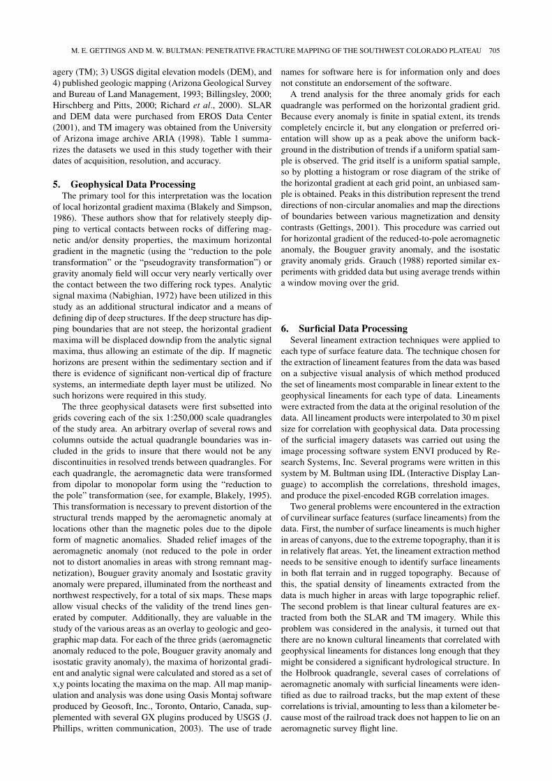
M. E. GETTINGS AND M. W. BULTMAN: PENETRATIVE FRACTURE MAPPING OF THE SOUTHWEST COLORADO PLATEAU 705
agery (TM); 3) USGS digital elevation models (DEM), and4) published geologic mapping (Arizona Geological Surveyand Bureau of Land Management, 1993; Billingsley, 2000;Hirschberg and Pitts, 2000; Richard et al., 2000). SLARand DEM data were purchased from EROS Data Center(2001), and TM imagery was obtained from the Universityof Arizona image archive ARIA (1998). Table 1 summa-rizes the datasets we used in this study together with theirdates of acquisition, resolution, and accuracy.
5. Geophysical Data ProcessingThe primary tool for this interpretation was the location
of local horizontal gradient maxima (Blakely and Simpson,1986). These authors show that for relatively steeply dip-ping to vertical contacts between rocks of differing mag-netic and/or density properties, the maximum horizontalgradient in the magnetic (using the “reduction to the poletransformation” or the “pseudogravity transformation”) orgravity anomaly field will occur very nearly vertically overthe contact between the two differing rock types. Analyticsignal maxima (Nabighian, 1972) have been utilized in thisstudy as an additional structural indicator and a means ofdefining dip of deep structures. If the deep structure has dip-ping boundaries that are not steep, the horizontal gradientmaxima will be displaced downdip from the analytic signalmaxima, thus allowing an estimate of the dip. If magnetichorizons are present within the sedimentary section and ifthere is evidence of significant non-vertical dip of fracturesystems, an intermediate depth layer must be utilized. Nosuch horizons were required in this study.
The three geophysical datasets were first subsetted intogrids covering each of the six 1:250,000 scale quadranglesof the study area. An arbitrary overlap of several rows andcolumns outside the actual quadrangle boundaries was in-cluded in the grids to insure that there would not be anydiscontinuities in resolved trends between quadrangles. Foreach quadrangle, the aeromagnetic data were transformedfrom dipolar to monopolar form using the “reduction tothe pole” transformation (see, for example, Blakely, 1995).This transformation is necessary to prevent distortion of thestructural trends mapped by the aeromagnetic anomaly atlocations other than the magnetic poles due to the dipoleform of magnetic anomalies. Shaded relief images of theaeromagnetic anomaly (not reduced to the pole in ordernot to distort anomalies in areas with strong remnant mag-netization), Bouguer gravity anomaly and Isostatic gravityanomaly were prepared, illuminated from the northeast andnorthwest respectively, for a total of six maps. These mapsallow visual checks of the validity of the trend lines gen-erated by computer. Additionally, they are valuable in thestudy of the various areas as an overlay to geologic and geo-graphic map data. For each of the three grids (aeromagneticanomaly reduced to the pole, Bouguer gravity anomaly andisostatic gravity anomaly), the maxima of horizontal gradi-ent and analytic signal were calculated and stored as a set ofx,y points locating the maxima on the map. All map manip-ulation and analysis was done using Oasis Montaj softwareproduced by Geosoft, Inc., Toronto, Ontario, Canada, sup-plemented with several GX plugins produced by USGS (J.Phillips, written communication, 2003). The use of trade
names for software here is for information only and doesnot constitute an endorsement of the software.
A trend analysis for the three anomaly grids for eachquadrangle was performed on the horizontal gradient grid.Because every anomaly is finite in spatial extent, its trendscompletely encircle it, but any elongation or preferred ori-entation will show up as a peak above the uniform back-ground in the distribution of trends if a uniform spatial sam-ple is observed. The grid itself is a uniform spatial sample,so by plotting a histogram or rose diagram of the strike ofthe horizontal gradient at each grid point, an unbiased sam-ple is obtained. Peaks in this distribution represent the trenddirections of non-circular anomalies and map the directionsof boundaries between various magnetization and densitycontrasts (Gettings, 2001). This procedure was carried outfor horizontal gradient of the reduced-to-pole aeromagneticanomaly, the Bouguer gravity anomaly, and the isostaticgravity anomaly grids. Grauch (1988) reported similar ex-periments with gridded data but using average trends withina window moving over the grid.
6. Surficial Data ProcessingSeveral lineament extraction techniques were applied to
each type of surface feature data. The technique chosen forthe extraction of lineament features from the data was basedon a subjective visual analysis of which method producedthe set of lineaments most comparable in linear extent to thegeophysical lineaments for each type of data. Lineamentswere extracted from the data at the original resolution of thedata. All lineament products were interpolated to 30 m pixelsize for correlation with geophysical data. Data processingof the surficial imagery datasets was carried out using theimage processing software system ENVI produced by Re-search Systems, Inc. Several programs were written in thissystem by M. Bultman using IDL (Interactive Display Lan-guage) to accomplish the correlations, threshold images,and produce the pixel-encoded RGB correlation images.
Two general problems were encountered in the extractionof curvilinear surface features (surface lineaments) from thedata. First, the number of surface lineaments is much higherin areas of canyons, due to the extreme topography, than it isin relatively flat areas. Yet, the lineament extraction methodneeds to be sensitive enough to identify surface lineamentsin both flat terrain and in rugged topography. Because ofthis, the spatial density of lineaments extracted from thedata is much higher in areas with large topographic relief.The second problem is that linear cultural features are ex-tracted from both the SLAR and TM imagery. While thisproblem was considered in the analysis, it turned out thatthere are no known cultural lineaments that correlated withgeophysical lineaments for distances long enough that theymight be considered a significant hydrological structure. Inthe Holbrook quadrangle, several cases of correlations ofaeromagnetic anomaly with surficial lineaments were iden-tified as due to railroad tracks, but the map extent of thesecorrelations is trivial, amounting to less than a kilometer be-cause most of the railroad track does not happen to lie on anaeromagnetic survey flight line.
706 M. E. GETTINGS AND M. W. BULTMAN: PENETRATIVE FRACTURE MAPPING OF THE SOUTHWEST COLORADO PLATEAU
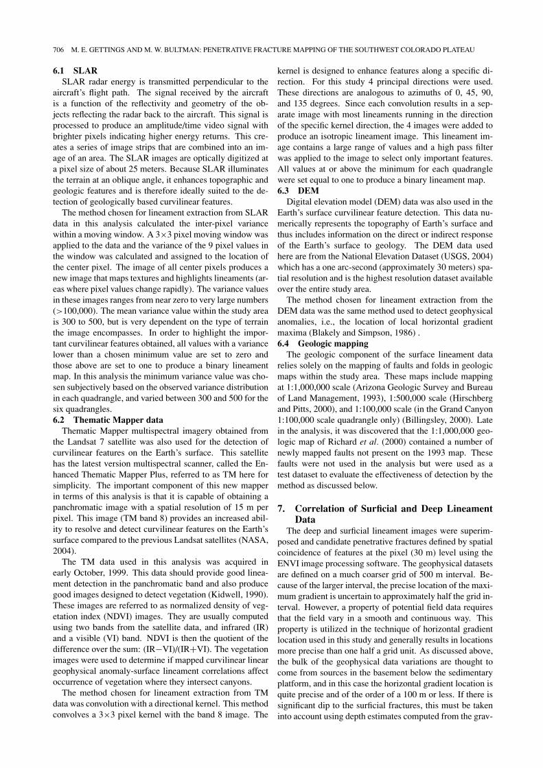
6.1 SLARSLAR radar energy is transmitted perpendicular to the
aircraft’s flight path. The signal received by the aircraftis a function of the reflectivity and geometry of the ob-jects reflecting the radar back to the aircraft. This signal isprocessed to produce an amplitude/time video signal withbrighter pixels indicating higher energy returns. This cre-ates a series of image strips that are combined into an im-age of an area. The SLAR images are optically digitized ata pixel size of about 25 meters. Because SLAR illuminatesthe terrain at an oblique angle, it enhances topographic andgeologic features and is therefore ideally suited to the de-tection of geologically based curvilinear features.
The method chosen for lineament extraction from SLARdata in this analysis calculated the inter-pixel variancewithin a moving window. A 3×3 pixel moving window wasapplied to the data and the variance of the 9 pixel values inthe window was calculated and assigned to the location ofthe center pixel. The image of all center pixels produces anew image that maps textures and highlights lineaments (ar-eas where pixel values change rapidly). The variance valuesin these images ranges from near zero to very large numbers(>100,000). The mean variance value within the study areais 300 to 500, but is very dependent on the type of terrainthe image encompasses. In order to highlight the impor-tant curvilinear features obtained, all values with a variancelower than a chosen minimum value are set to zero andthose above are set to one to produce a binary lineamentmap. In this analysis the minimum variance value was cho-sen subjectively based on the observed variance distributionin each quadrangle, and varied between 300 and 500 for thesix quadrangles.6.2 Thematic Mapper data
Thematic Mapper multispectral imagery obtained fromthe Landsat 7 satellite was also used for the detection ofcurvilinear features on the Earth’s surface. This satellitehas the latest version multispectral scanner, called the En-hanced Thematic Mapper Plus, referred to as TM here forsimplicity. The important component of this new mapperin terms of this analysis is that it is capable of obtaining apanchromatic image with a spatial resolution of 15 m perpixel. This image (TM band 8) provides an increased abil-ity to resolve and detect curvilinear features on the Earth’ssurface compared to the previous Landsat satellites (NASA,2004).
The TM data used in this analysis was acquired inearly October, 1999. This data should provide good linea-ment detection in the panchromatic band and also producegood images designed to detect vegetation (Kidwell, 1990).These images are referred to as normalized density of veg-etation index (NDVI) images. They are usually computedusing two bands from the satellite data, and infrared (IR)and a visible (VI) band. NDVI is then the quotient of thedifference over the sum: (IR−VI)/(IR+VI). The vegetationimages were used to determine if mapped curvilinear lineargeophysical anomaly-surface lineament correlations affectoccurrence of vegetation where they intersect canyons.
The method chosen for lineament extraction from TMdata was convolution with a directional kernel. This methodconvolves a 3×3 pixel kernel with the band 8 image. The
kernel is designed to enhance features along a specific di-rection. For this study 4 principal directions were used.These directions are analogous to azimuths of 0, 45, 90,and 135 degrees. Since each convolution results in a sep-arate image with most lineaments running in the directionof the specific kernel direction, the 4 images were added toproduce an isotropic lineament image. This lineament im-age contains a large range of values and a high pass filterwas applied to the image to select only important features.All values at or above the minimum for each quadranglewere set equal to one to produce a binary lineament map.6.3 DEM
Digital elevation model (DEM) data was also used in theEarth’s surface curvilinear feature detection. This data nu-merically represents the topography of Earth’s surface andthus includes information on the direct or indirect responseof the Earth’s surface to geology. The DEM data usedhere are from the National Elevation Dataset (USGS, 2004)which has a one arc-second (approximately 30 meters) spa-tial resolution and is the highest resolution dataset availableover the entire study area.
The method chosen for lineament extraction from theDEM data was the same method used to detect geophysicalanomalies, i.e., the location of local horizontal gradientmaxima (Blakely and Simpson, 1986) .6.4 Geologic mapping
The geologic component of the surface lineament datarelies solely on the mapping of faults and folds in geologicmaps within the study area. These maps include mappingat 1:1,000,000 scale (Arizona Geologic Survey and Bureauof Land Management, 1993), 1:500,000 scale (Hirschbergand Pitts, 2000), and 1:100,000 scale (in the Grand Canyon1:100,000 scale quadrangle only) (Billingsley, 2000). Latein the analysis, it was discovered that the 1:1,000,000 geo-logic map of Richard et al. (2000) contained a number ofnewly mapped faults not present on the 1993 map. Thesefaults were not used in the analysis but were used as atest dataset to evaluate the effectiveness of detection by themethod as discussed below.
7. Correlation of Surficial and Deep LineamentData
The deep and surficial lineament images were superim-posed and candidate penetrative fractures defined by spatialcoincidence of features at the pixel (30 m) level using theENVI image processing software. The geophysical datasetsare defined on a much coarser grid of 500 m interval. Be-cause of the larger interval, the precise location of the maxi-mum gradient is uncertain to approximately half the grid in-terval. However, a property of potential field data requiresthat the field vary in a smooth and continuous way. Thisproperty is utilized in the technique of horizontal gradientlocation used in this study and generally results in locationsmore precise than one half a grid unit. As discussed above,the bulk of the geophysical data variations are thought tocome from sources in the basement below the sedimentaryplatform, and in this case the horizontal gradient location isquite precise and of the order of a 100 m or less. If there issignificant dip to the surficial fractures, this must be takeninto account using depth estimates computed from the grav-
M. E. GETTINGS AND M. W. BULTMAN: PENETRATIVE FRACTURE MAPPING OF THE SOUTHWEST COLORADO PLATEAU 707
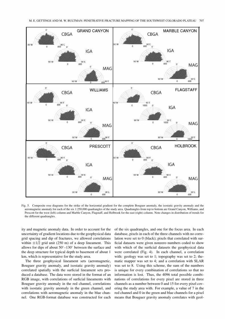
Fig. 5. Composite rose diagrams for the strike of the horizontal gradient for the complete Bouguer anomaly, the isostatic gravity anomaly and theaeromagnetic anomaly for each of the six 1:250,000 quadrangles of the study area. Quadrangles from top to bottom are Grand Canyon, Williams, andPrescott for the west (left) column and Marble Canyon, Flagstaff, and Holbrook for the east (right) column. Note changes in distribution of trends forthe different quadrangles.
ity and magnetic anomaly data. In order to account for theuncertainty of gradient locations due to the geophysical datagrid spacing and dip of fractures, we allowed correlationswithin ±1/2 grid unit (250 m) of a deep lineament. Thisallows for dips of about 50◦–130◦ between the surface andthe deep structure for typical depth to basement of about 1km, which is representative for the study area.
The three geophysical lineament sets (aeromagnetic,Bouguer gravity anomaly, and isostatic gravity anomaly)correlated spatially with the surficial lineament sets pro-duced a database. The data were stored in the format of anRGB image, with correlations of surficial lineaments withBouguer gravity anomaly in the red channel, correlationswith isostatic gravity anomaly in the green channel, andcorrelations with aeromagnetic anomaly in the blue chan-nel. One RGB-format database was constructed for each
of the six quadrangles, and one for the focus area. In eachdatabase, pixels in each of the three channels with no corre-lation were set to 0 (black); pixels that correlated with sur-ficial datasets were given nonzero numbers coded to showwith which of the surficial datasets the geophysical datawere correlated (Fig. 4). In each channel, a correlationwith: geology was set to 1; topography was set to 2; the-matic mapper was set to 4; and a correlation with SLARwas set to 8. Using this scheme, the sum of the numbersis unique for every combination of correlations so that noinformation is lost. Thus, the 4096 total possible combi-nations of correlations for every pixel are stored in threechannels as a number between 0 and 15 for every pixel cov-ering the study area with. For example, a value of 7 in thered channel and 0 in the green and blue channels for a pixelmeans that Bouguer gravity anomaly correlates with geol-
708 M. E. GETTINGS AND M. W. BULTMAN: PENETRATIVE FRACTURE MAPPING OF THE SOUTHWEST COLORADO PLATEAU
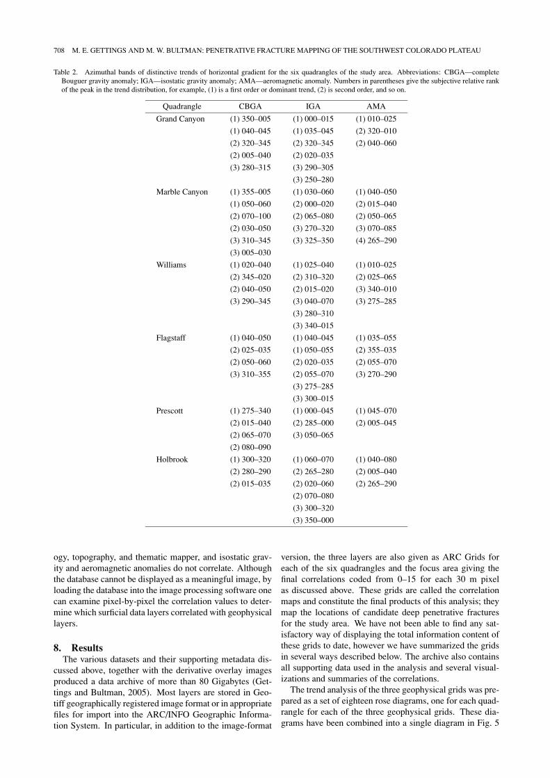
Table 2. Azimuthal bands of distinctive trends of horizontal gradient for the six quadrangles of the study area. Abbreviations: CBGA—completeBouguer gravity anomaly; IGA—isostatic gravity anomaly; AMA—aeromagnetic anomaly. Numbers in parentheses give the subjective relative rankof the peak in the trend distribution, for example, (1) is a first order or dominant trend, (2) is second order, and so on.
Quadrangle CBGA IGA AMA
Grand Canyon (1) 350–005 (1) 000–015 (1) 010–025
(1) 040–045 (1) 035–045 (2) 320–010
(2) 320–345 (2) 320–345 (2) 040–060
(2) 005–040 (2) 020–035
(3) 280–315 (3) 290–305
(3) 250–280
Marble Canyon (1) 355–005 (1) 030–060 (1) 040–050
(1) 050–060 (2) 000–020 (2) 015–040
(2) 070–100 (2) 065–080 (2) 050–065
(2) 030–050 (3) 270–320 (3) 070–085
(3) 310–345 (3) 325–350 (4) 265–290
(3) 005–030
Williams (1) 020–040 (1) 025–040 (1) 010–025
(2) 345–020 (2) 310–320 (2) 025–065
(2) 040–050 (2) 015–020 (3) 340–010
(3) 290–345 (3) 040–070 (3) 275–285
(3) 280–310
(3) 340–015
Flagstaff (1) 040–050 (1) 040–045 (1) 035–055
(2) 025–035 (1) 050–055 (2) 355–035
(2) 050–060 (2) 020–035 (2) 055–070
(3) 310–355 (2) 055–070 (3) 270–290
(3) 275–285
(3) 300–015
Prescott (1) 275–340 (1) 000–045 (1) 045–070
(2) 015–040 (2) 285–000 (2) 005–045
(2) 065–070 (3) 050–065
(2) 080–090
Holbrook (1) 300–320 (1) 060–070 (1) 040–080
(2) 280–290 (2) 265–280 (2) 005–040
(2) 015–035 (2) 020–060 (2) 265–290
(2) 070–080
(3) 300–320
(3) 350–000
ogy, topography, and thematic mapper, and isostatic grav-ity and aeromagnetic anomalies do not correlate. Althoughthe database cannot be displayed as a meaningful image, byloading the database into the image processing software onecan examine pixel-by-pixel the correlation values to deter-mine which surficial data layers correlated with geophysicallayers.
8. ResultsThe various datasets and their supporting metadata dis-
cussed above, together with the derivative overlay imagesproduced a data archive of more than 80 Gigabytes (Get-tings and Bultman, 2005). Most layers are stored in Geo-tiff geographically registered image format or in appropriatefiles for import into the ARC/INFO Geographic Informa-tion System. In particular, in addition to the image-format
version, the three layers are also given as ARC Grids foreach of the six quadrangles and the focus area giving thefinal correlations coded from 0–15 for each 30 m pixelas discussed above. These grids are called the correlationmaps and constitute the final products of this analysis; theymap the locations of candidate deep penetrative fracturesfor the study area. We have not been able to find any sat-isfactory way of displaying the total information content ofthese grids to date, however we have summarized the gridsin several ways described below. The archive also containsall supporting data used in the analysis and several visual-izations and summaries of the correlations.
The trend analysis of the three geophysical grids was pre-pared as a set of eighteen rose diagrams, one for each quad-rangle for each of the three geophysical grids. These dia-grams have been combined into a single diagram in Fig. 5
M. E. GETTINGS AND M. W. BULTMAN: PENETRATIVE FRACTURE MAPPING OF THE SOUTHWEST COLORADO PLATEAU 709
with the rose diagrams plotted in the map position of thequadrangle to which they apply. This enables comparison ofthe diagrams with the geologic map of Fig. 2. Table 2 liststhe ranked trend set directions determined by the authorsfrom study of Fig. 5 for these diagrams for each anomalytype and each quadrangle.
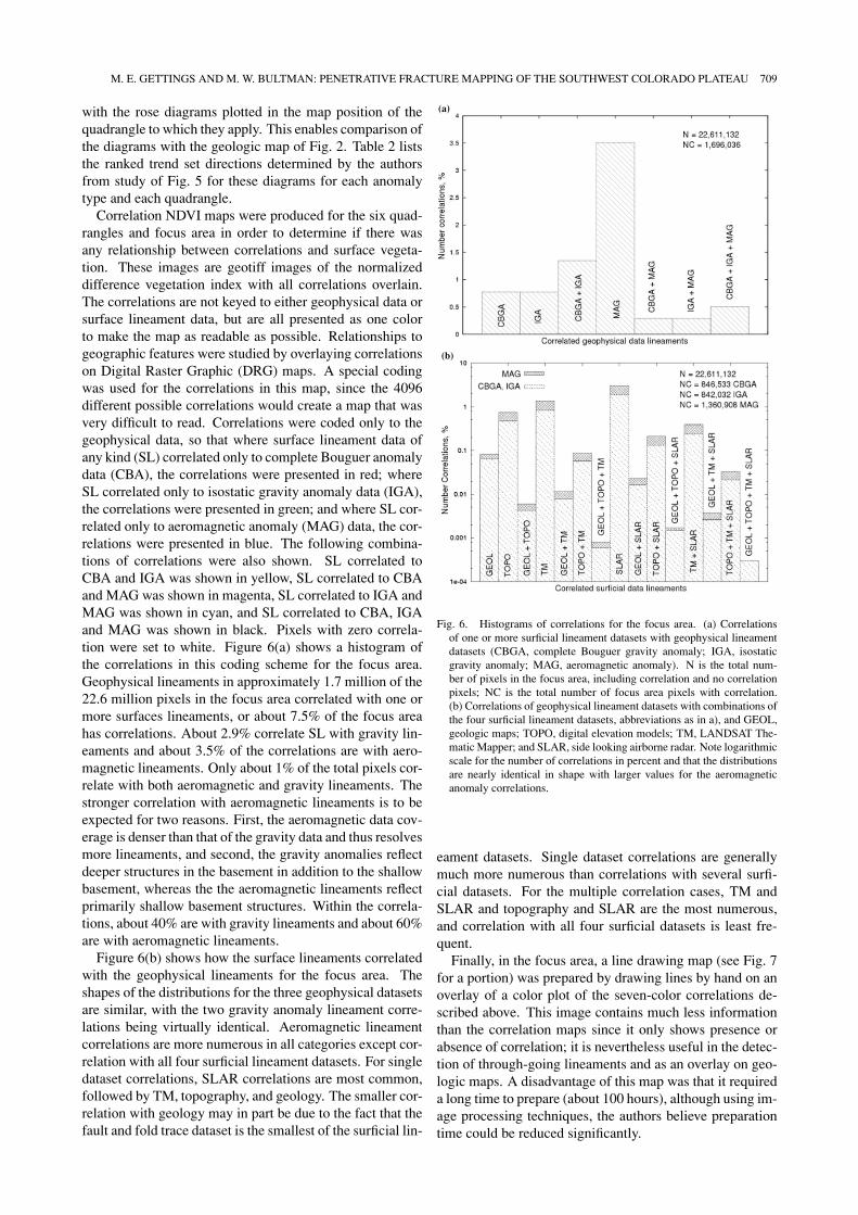
Correlation NDVI maps were produced for the six quad-rangles and focus area in order to determine if there wasany relationship between correlations and surface vegeta-tion. These images are geotiff images of the normalizeddifference vegetation index with all correlations overlain.The correlations are not keyed to either geophysical data orsurface lineament data, but are all presented as one colorto make the map as readable as possible. Relationships togeographic features were studied by overlaying correlationson Digital Raster Graphic (DRG) maps. A special codingwas used for the correlations in this map, since the 4096different possible correlations would create a map that wasvery difficult to read. Correlations were coded only to thegeophysical data, so that where surface lineament data ofany kind (SL) correlated only to complete Bouguer anomalydata (CBA), the correlations were presented in red; whereSL correlated only to isostatic gravity anomaly data (IGA),the correlations were presented in green; and where SL cor-related only to aeromagnetic anomaly (MAG) data, the cor-relations were presented in blue. The following combina-tions of correlations were also shown. SL correlated toCBA and IGA was shown in yellow, SL correlated to CBAand MAG was shown in magenta, SL correlated to IGA andMAG was shown in cyan, and SL correlated to CBA, IGAand MAG was shown in black. Pixels with zero correla-tion were set to white. Figure 6(a) shows a histogram ofthe correlations in this coding scheme for the focus area.Geophysical lineaments in approximately 1.7 million of the22.6 million pixels in the focus area correlated with one ormore surfaces lineaments, or about 7.5% of the focus areahas correlations. About 2.9% correlate SL with gravity lin-eaments and about 3.5% of the correlations are with aero-magnetic lineaments. Only about 1% of the total pixels cor-relate with both aeromagnetic and gravity lineaments. Thestronger correlation with aeromagnetic lineaments is to beexpected for two reasons. First, the aeromagnetic data cov-erage is denser than that of the gravity data and thus resolvesmore lineaments, and second, the gravity anomalies reflectdeeper structures in the basement in addition to the shallowbasement, whereas the the aeromagnetic lineaments reflectprimarily shallow basement structures. Within the correla-tions, about 40% are with gravity lineaments and about 60%are with aeromagnetic lineaments.
Figure 6(b) shows how the surface lineaments correlatedwith the geophysical lineaments for the focus area. Theshapes of the distributions for the three geophysical datasetsare similar, with the two gravity anomaly lineament corre-lations being virtually identical. Aeromagnetic lineamentcorrelations are more numerous in all categories except cor-relation with all four surficial lineament datasets. For singledataset correlations, SLAR correlations are most common,followed by TM, topography, and geology. The smaller cor-relation with geology may in part be due to the fact that thefault and fold trace dataset is the smallest of the surficial lin-
(a)
(b)
Fig. 6. Histograms of correlations for the focus area. (a) Correlationsof one or more surficial lineament datasets with geophysical lineamentdatasets (CBGA, complete Bouguer gravity anomaly; IGA, isostaticgravity anomaly; MAG, aeromagnetic anomaly). N is the total num-ber of pixels in the focus area, including correlation and no correlationpixels; NC is the total number of focus area pixels with correlation.(b) Correlations of geophysical lineament datasets with combinations ofthe four surficial lineament datasets, abbreviations as in a), and GEOL,geologic maps; TOPO, digital elevation models; TM, LANDSAT The-matic Mapper; and SLAR, side looking airborne radar. Note logarithmicscale for the number of correlations in percent and that the distributionsare nearly identical in shape with larger values for the aeromagneticanomaly correlations.
eament datasets. Single dataset correlations are generallymuch more numerous than correlations with several surfi-cial datasets. For the multiple correlation cases, TM andSLAR and topography and SLAR are the most numerous,and correlation with all four surficial datasets is least fre-quent.
Finally, in the focus area, a line drawing map (see Fig. 7for a portion) was prepared by drawing lines by hand on anoverlay of a color plot of the seven-color correlations de-scribed above. This image contains much less informationthan the correlation maps since it only shows presence orabsence of correlation; it is nevertheless useful in the detec-tion of through-going lineaments and as an overlay on geo-logic maps. A disadvantage of this map was that it requireda long time to prepare (about 100 hours), although using im-age processing techniques, the authors believe preparationtime could be reduced significantly.
710 M. E. GETTINGS AND M. W. BULTMAN: PENETRATIVE FRACTURE MAPPING OF THE SOUTHWEST COLORADO PLATEAU
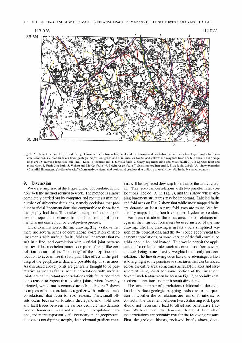
Fig. 7. Northwest quarter of the line drawing of correlations between deep- and shallow-lineament datasets for the focus area (see Figs. 1 and 2 for focusarea location). Colored lines are from geologic maps: red, green and blue lines are faults; and yellow and magenta lines are fold axes. Thin orangelines are 15′ latitude-longitude grid lines. Labeled features are; 1, Sinyala fault; 2, Crazy Jug monocline and Muav fault; 3, Big Springs fault andmonocline; 4, Uncle Jim fault; 5, Vishnu and McKee faults; 6, Bright Angel fault; 7, Supai monocline; and 8, Slate fault. Labels “A” show examplesof parallel lineaments (“railroad tracks”) from analytic signal and horizontal gradient that indicate more shallow dip in the basement contacts.
9. DiscussionWe were surprised at the large number of correlations and
how well the method seemed to work. The method is almostcompletely carried out by computer and requires a minimalnumber of subjective decisions, namely decisions that pro-duce surficial lineament densities comparable to those fromthe geophysical data. This makes the approach quite objec-tive and repeatable because the actual delineation of linea-ments is not carried out by a subjective process.
Close examination of the line drawing (Fig. 7) shows thatthere are several kinds of correlation: correlation of deeplineaments with surficial faults, folds or lineaments that re-sult in a line, and correlation with surficial joint patternsthat result in en echelon patterns or paths of joint-like cor-relation because of the “smearing” of the deep lineamentlocation to account for the low-pass filter effect of the grid-ding of the geophysical data and possible dip of structures.As discussed above, joints are generally thought to be pen-etrative as well as faults, so that correlations with surficialjoints are as important as correlations with faults and thereis no reason to expect that existing joints, when favorablyoriented, would not accommodate offset. Figure 7 showsexamples of both correlations together with “railroad trackcorrelations” that occur for two reasons. First, small off-sets occur because of location discrepancies of fold axesand fault traces between the various geologic map datasetsfrom differences in scale and accuracy of compilation. Sec-ond, and more importantly, if a boundary in the geophysicaldatasets is not dipping steeply, the horizontal gradient max-
ima will be displaced downdip from that of the analytic sig-nal. This results in correlations with two parallel lines (seelocations labeled “A” in Fig. 7), and thus show where dip-ping basement structures may be important. Labeled faultsand fold axes on Fig. 7 show that while most mapped faultsare detected at least in part, fold axes are much less fre-quently mapped and often have no geophysical expression.
For areas outside of the focus area, the correlations im-ages in their various forms can be used instead of the linedrawing. The line drawing is in fact a very simplified ver-sion of the correlations, and the 0–7 coded geophysical lin-eaments correlations, or some version of the full correlationgrids, should be used instead. This would permit the appli-cation of correlation rules such as correlations from severaldatasets being more heavily weighted than only one cor-relation. The line drawing does have one advantage, whichis to highlight some penetrative structures that can be tracedacross the entire area, sometimes as fault/fold axes and else-where utilizing joints for some portion of the lineament.Several such features can be seen on Fig. 7, especially east-northeast directions and north-south directions.
The large number of correlations additional to those de-fined in surface geologic mapping leads one to the ques-tion of whether the correlations are real or fortuitous. Acontact in the basement between two contrasting rock typesshould not necessarily lead to offset and penetrative frac-ture. We have concluded, however, that most if not all ofthe correlations are probably real for the following reasons.First, the geologic history, reviewed briefly above, docu-
M. E. GETTINGS AND M. W. BULTMAN: PENETRATIVE FRACTURE MAPPING OF THE SOUTHWEST COLORADO PLATEAU 711
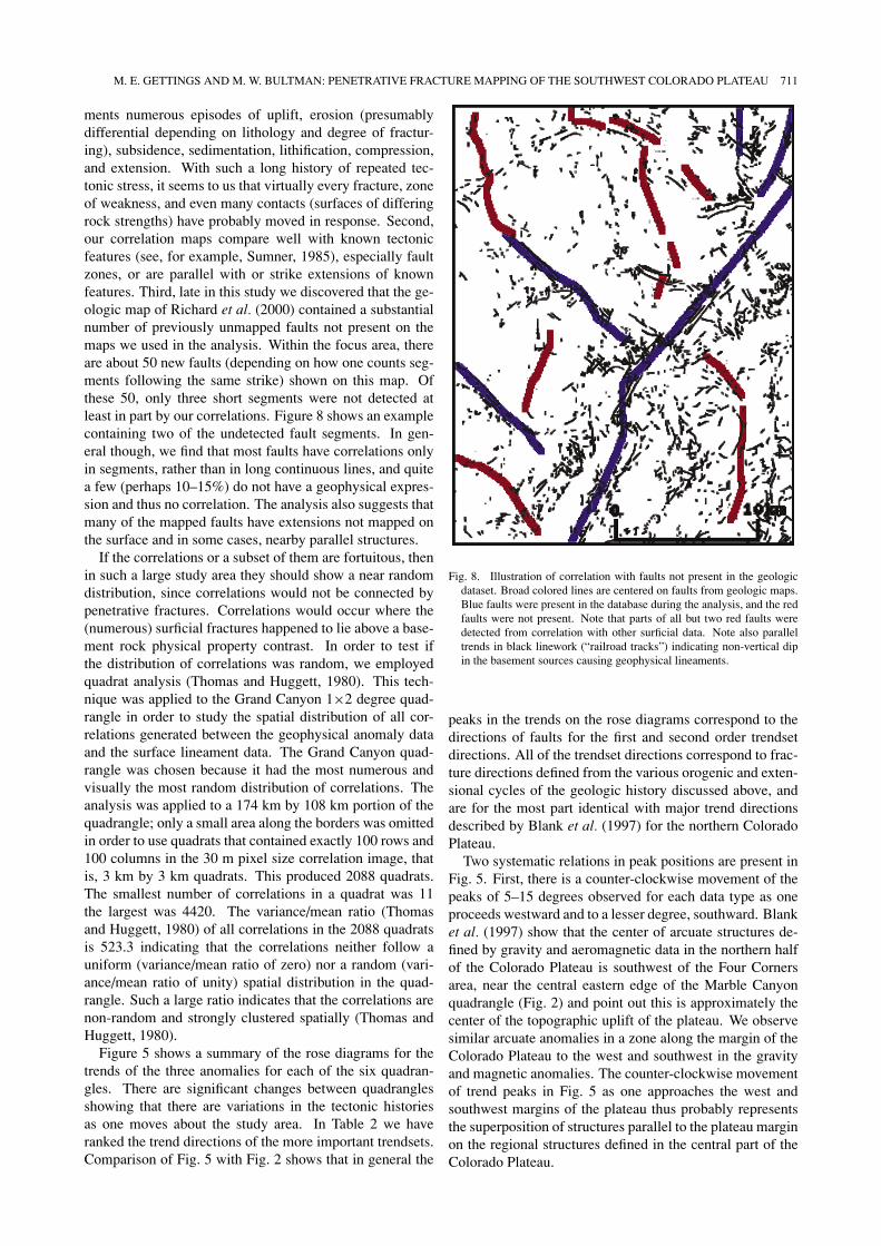
ments numerous episodes of uplift, erosion (presumablydifferential depending on lithology and degree of fractur-ing), subsidence, sedimentation, lithification, compression,and extension. With such a long history of repeated tec-tonic stress, it seems to us that virtually every fracture, zoneof weakness, and even many contacts (surfaces of differingrock strengths) have probably moved in response. Second,our correlation maps compare well with known tectonicfeatures (see, for example, Sumner, 1985), especially faultzones, or are parallel with or strike extensions of knownfeatures. Third, late in this study we discovered that the ge-ologic map of Richard et al. (2000) contained a substantialnumber of previously unmapped faults not present on themaps we used in the analysis. Within the focus area, thereare about 50 new faults (depending on how one counts seg-ments following the same strike) shown on this map. Ofthese 50, only three short segments were not detected atleast in part by our correlations. Figure 8 shows an examplecontaining two of the undetected fault segments. In gen-eral though, we find that most faults have correlations onlyin segments, rather than in long continuous lines, and quitea few (perhaps 10–15%) do not have a geophysical expres-sion and thus no correlation. The analysis also suggests thatmany of the mapped faults have extensions not mapped onthe surface and in some cases, nearby parallel structures.
If the correlations or a subset of them are fortuitous, thenin such a large study area they should show a near randomdistribution, since correlations would not be connected bypenetrative fractures. Correlations would occur where the(numerous) surficial fractures happened to lie above a base-ment rock physical property contrast. In order to test ifthe distribution of correlations was random, we employedquadrat analysis (Thomas and Huggett, 1980). This tech-nique was applied to the Grand Canyon 1×2 degree quad-rangle in order to study the spatial distribution of all cor-relations generated between the geophysical anomaly dataand the surface lineament data. The Grand Canyon quad-rangle was chosen because it had the most numerous andvisually the most random distribution of correlations. Theanalysis was applied to a 174 km by 108 km portion of thequadrangle; only a small area along the borders was omittedin order to use quadrats that contained exactly 100 rows and100 columns in the 30 m pixel size correlation image, thatis, 3 km by 3 km quadrats. This produced 2088 quadrats.The smallest number of correlations in a quadrat was 11the largest was 4420. The variance/mean ratio (Thomasand Huggett, 1980) of all correlations in the 2088 quadratsis 523.3 indicating that the correlations neither follow auniform (variance/mean ratio of zero) nor a random (vari-ance/mean ratio of unity) spatial distribution in the quad-rangle. Such a large ratio indicates that the correlations arenon-random and strongly clustered spatially (Thomas andHuggett, 1980).
Figure 5 shows a summary of the rose diagrams for thetrends of the three anomalies for each of the six quadran-gles. There are significant changes between quadranglesshowing that there are variations in the tectonic historiesas one moves about the study area. In Table 2 we haveranked the trend directions of the more important trendsets.Comparison of Fig. 5 with Fig. 2 shows that in general the
Fig. 8. Illustration of correlation with faults not present in the geologicdataset. Broad colored lines are centered on faults from geologic maps.Blue faults were present in the database during the analysis, and the redfaults were not present. Note that parts of all but two red faults weredetected from correlation with other surficial data. Note also paralleltrends in black linework (“railroad tracks”) indicating non-vertical dipin the basement sources causing geophysical lineaments.
peaks in the trends on the rose diagrams correspond to thedirections of faults for the first and second order trendsetdirections. All of the trendset directions correspond to frac-ture directions defined from the various orogenic and exten-sional cycles of the geologic history discussed above, andare for the most part identical with major trend directionsdescribed by Blank et al. (1997) for the northern ColoradoPlateau.
Two systematic relations in peak positions are present inFig. 5. First, there is a counter-clockwise movement of thepeaks of 5–15 degrees observed for each data type as oneproceeds westward and to a lesser degree, southward. Blanket al. (1997) show that the center of arcuate structures de-fined by gravity and aeromagnetic data in the northern halfof the Colorado Plateau is southwest of the Four Cornersarea, near the central eastern edge of the Marble Canyonquadrangle (Fig. 2) and point out this is approximately thecenter of the topographic uplift of the plateau. We observesimilar arcuate anomalies in a zone along the margin of theColorado Plateau to the west and southwest in the gravityand magnetic anomalies. The counter-clockwise movementof trend peaks in Fig. 5 as one approaches the west andsouthwest margins of the plateau thus probably representsthe superposition of structures parallel to the plateau marginon the regional structures defined in the central part of theColorado Plateau.
712 M. E. GETTINGS AND M. W. BULTMAN: PENETRATIVE FRACTURE MAPPING OF THE SOUTHWEST COLORADO PLATEAU
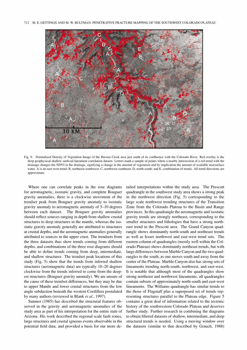
Fig. 9. Normalized Density of Vegetation Image of the Havasu Creek area just south of its confluence with the Colorado River. Red overlay is thedeep geophysical-shallow surficial lineament correlation dataset. Letters mark a sample of points where a nearby intersection of a red trend with thedrainage changes the NDVI in the drainage, signifying a change in the amount of vegetation and by implication the amount of available nearsurfacewater. A is an east-west trend; B, northeast-southwest; C, northwest-southeast; D, north-south; and E, combination of trends. All trend directions areapproximate.
Where one can correlate peaks in the rose diagramsfor aeromagnetic, isostatic gravity, and complete Bouguergravity anomalies, there is a clockwise movement of thetrendset peak from Bouguer gravity anomaly to isostaticgravity anomaly to aeromagnetic anomaly of 5–10 degreesbetween each dataset. The Bouguer gravity anomaliesshould reflect sources ranging in depth from shallow crustalstructures to deep structures in the mantle, whereas the iso-static gravity anomaly generally are attributed to structuresat crustal depths, and the aeromagnetic anomalies generallyattributed to sources in the upper crust. The trendsets fromthe three datasets thus show trends coming from differentdepths, and combinations of the three rose diagrams shouldbe able to define trends coming from deep, intermediate,and shallow structures. The trendset peak locations of thisstudy (Fig. 5) show that the trends from inferred shallowstructures (aeromagnetic data) are typically 10–20 degreesclockwise from the trends inferred to come from the deep-est structures (Bouguer gravity anomaly). We are unsure ofthe cause of these trendset differences, but they may be dueto upper Mantle and lower crustal structures from the lowangle subduction beneath the western Cordillera postulatedby many authors (reviewed in Blank et al., 1997).
Sumner (1985) has described the structural features ob-served in the gravity and aeromagnetic anomalies of thestudy area as part of his interpretation for the entire state ofArizona. His work described the regional scale fault zones,large structures and crustal igneous events observable in thepotential field data, and provided a basis for our more de-
tailed interpretations within the study area. The Prescottquadrangle in the southwest study area shows a strong peakin the northwest direction (Fig. 5) corresponding to thelarge scale northwest trending structures of the TransitionZone from the Colorado Plateau to the Basin and Rangeprovinces. In this quadrangle the aeromagnetic and isostaticgravity trends are strongly northeast, corresponding to thesmaller structures and lithologies that have a strong north-east trend in the Prescott area. The Grand Canyon quad-rangle shows dominantly north-south and northeast trendsas well as lesser northwest and east-west trend sets. Theeastern column of quadrangles (mostly well within the Col-orado Plateau) shows dominantly northeast trends, but withlarge differences between Marble Canyon and the two quad-rangles to the south, as one moves south and away from thecenter of the Plateau. Marble Canyon also has strong sets oflineaments trending north-south, northwest, and east-west.It is notable that although most of the quadrangles showstrong northeast and northwest lineaments, all quadranglescontain subsets of approximately north-south and east-westlineaments. The Williams quadrangle has similar trends tothe those of Flagstaff plus a superposed set of trends rep-resenting structures parallel to the Plateau edge. Figure 5contains a great deal of information related to the tectonichistory of the southwestern Colorado Plateau and deservesfurther study. Further research in combining the diagramsto obtain filtered datasets of shallow, intermediate, and deepstructural trends is needed. Using a moving window overthe datasets (similar to that described by Grauch, 1988)
M. E. GETTINGS AND M. W. BULTMAN: PENETRATIVE FRACTURE MAPPING OF THE SOUTHWEST COLORADO PLATEAU 713
would define continuous variations of the trendsets in a wayuseful for regional tectonic studies.
Blank et al. (1997) have observed a distinct set ofstructures in a band overlapping the northern ColoradoPlateau margins and the surrounding extensional provinces.They suggest that these structures may represent gravi-tational collapse radially outward from the center of up-lifted Plateau, and that there may be magmatic infilling be-tween the blocks of Precambrian basement in this zone ofoutward extension. We see evidence for the same typesof arcuate structures in the geophysical anomalies of thestudy area along the western and southwestern Plateau mar-gin. Force (1997) has documented 7 km of Eocene mag-matic thickening in the Santa Catalina core complex offthe south-southwest margin of the Plateau, and Gettings(1996) showed that “rafting” of the Whetstone Mountainsby a subsurface Tertiary intrusive was the only simple wayto explain the aeromagnetic and gravity anomalies. Get-tings (1994) suggested that magmatic infilling between ex-tended basement blocks was a major cause of the regionalaeromagnetic and gravity anomalies in southeastern Ari-zona. These magmatic events are essentially contempora-neous with the timing of uplift of the Plateau (about one kmpost-Laramide Paleogene uplift and about three km Neo-gene uplift, reviewed in Blank et al., 1997).
Images showing the derived deep- and shallow-data cor-relations superimposed on the NDVI images show clearlythat many correlated lineaments are controlling surface wa-ters (an example is shown in Fig. 9). We infer that structurescorresponding to the correlated lineaments are dammingnear-surface water or creating springs in drainages so thatwater is held sufficiently close to the surface to supportvegetation, thus producing whiter portions of the drainage.In areas where the structure appears to abruptly cut off theNDVI downstream, we infer that the structure intercepts thedrainage and takes the water to deeper depths so that thereis little or no vegetation downstream. The controls by east-west lineaments is somewhat surprising as the east-west lin-eaments were thought to be a fabric in the basement butare not obvious on the surface without the methods of thisstudy. Numerous cases can be seen on Fig. 9 where whitersections of drainages are bounded by intersecting correla-tions. On the other hand, there are several areas of vegeta-tion that do not show any control by correlations and thusare apparently not related to deeper structures. The NDVIimages also are a convenient means of locating springs andseeps that have substantial associated vegetation within theGrand Canyon.
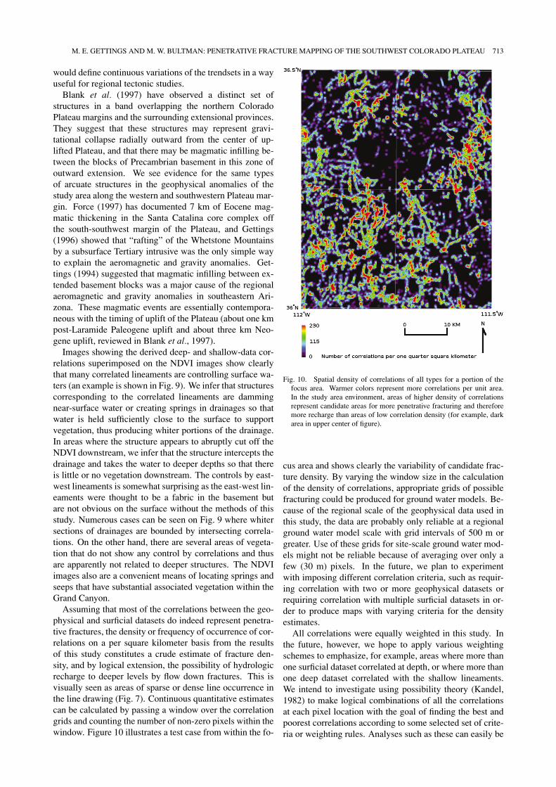
Assuming that most of the correlations between the geo-physical and surficial datasets do indeed represent penetra-tive fractures, the density or frequency of occurrence of cor-relations on a per square kilometer basis from the resultsof this study constitutes a crude estimate of fracture den-sity, and by logical extension, the possibility of hydrologicrecharge to deeper levels by flow down fractures. This isvisually seen as areas of sparse or dense line occurrence inthe line drawing (Fig. 7). Continuous quantitative estimatescan be calculated by passing a window over the correlationgrids and counting the number of non-zero pixels within thewindow. Figure 10 illustrates a test case from within the fo-
Fig. 10. Spatial density of correlations of all types for a portion of thefocus area. Warmer colors represent more correlations per unit area.In the study area environment, areas of higher density of correlationsrepresent candidate areas for more penetrative fracturing and thereforemore recharge than areas of low correlation density (for example, darkarea in upper center of figure).
cus area and shows clearly the variability of candidate frac-ture density. By varying the window size in the calculationof the density of correlations, appropriate grids of possiblefracturing could be produced for ground water models. Be-cause of the regional scale of the geophysical data used inthis study, the data are probably only reliable at a regionalground water model scale with grid intervals of 500 m orgreater. Use of these grids for site-scale ground water mod-els might not be reliable because of averaging over only afew (30 m) pixels. In the future, we plan to experimentwith imposing different correlation criteria, such as requir-ing correlation with two or more geophysical datasets orrequiring correlation with multiple surficial datasets in or-der to produce maps with varying criteria for the densityestimates.
All correlations were equally weighted in this study. Inthe future, however, we hope to apply various weightingschemes to emphasize, for example, areas where more thanone surficial dataset correlated at depth, or where more thanone deep dataset correlated with the shallow lineaments.We intend to investigate using possibility theory (Kandel,1982) to make logical combinations of all the correlationsat each pixel location with the goal of finding the best andpoorest correlations according to some selected set of crite-ria or weighting rules. Analyses such as these can easily be
714 M. E. GETTINGS AND M. W. BULTMAN: PENETRATIVE FRACTURE MAPPING OF THE SOUTHWEST COLORADO PLATEAU
carried out using the grids that give the pixel-by-pixel corre-lations for the aeromagnetic, Bouguer gravity and isostaticanomalies.
10. ConclusionThe methods used in this study objectively and repeat-
ably locate a subset of deep penetrative fracture candi-dates. They do not, however, provide any information asto whether any fracture is open or closed. In some cases,time domain electrical sounding can detect whether or not aparticular fracture is water-filled or not, however there is atpresent no method to survey large areas such as the area ofthis study for reasonable costs. It is also to be rememberedthat if a structure in the basement does not juxtapose rocksof differing density or magnetization, there will be no geo-physical anomaly and thus no deep lineament to correlatewith surface lineaments. Because of this and lack of de-tailed spatial data coverage, there are probably many moredeep penetrative fractures than mapped by this study. Allof the important deep fracture directions detected by thisstudy are accounted for by known tectonic events in the ge-ologic history. This study has, however, mapped many ex-tensions of known structures and delineated numerous newstructures parallel to known ones.
The correlation maps produced in this study provide amap of the tectonic fabric for the Southwestern ColoradoPlateau and the interpretation of this fabric will be a fruitfularea of research. We believe the results presented here pointto a complex history of plateau uplift and radial horizontalextension in a broad transition zone around the margins ofthe Plateau.
The method described here yields a subset of candidatesof deep penetrative fractures except for coincidental corre-lations. We have shown that the distribution of correlationsis highly clustered and non-random, and thus most corre-lations are unlikely to be coincidental. The locations ofcandidate deep fractures are presented at a resolution (pixelsize) of 30 m, but are subject to errors in location of upto plus or minus 250 m due to the 500 m grid interval ofthe geophysical data defining the location of deep structuralboundaries. Numerous new zones of deep fracturing pos-sibility have been defined and are archived in digital gridsthat uniquely define which deep and shallow datasets cor-relate. Once threshold parameters are chosen for the linea-ment extraction algorithms, the procedure is objective andrepeatable.
The inferred structures appear to also control near-surface water movement in some cases. The spatial densityof correlations (Fig. 10) gives a starting approximation ofareas of poor and good recharge possibility due to deep frac-ture density. Finally, possibility theory from fuzzy logic,or some other schema of criteria, could be used to furtherquantify and discriminate the correlations.
Acknowledgments. This work was funded by the United StatesNational Park Service Water Resources Division, Fort Collins,Colorado. A discussion with William Steinkampf of the Wa-ter Resources Division, U.S. Geological Survey, resulted in theconcept for this study. We are indebted to numerous colleaguesfor helpful discussions and to Christopher Call for website de-sign and construction of the database. Richard Blakely and
Richard Saltus of the U.S. Geological Survey reviewed an earlyversion of the manuscript and provided numerous helpful com-ments. Abe Springer, Dean Kleinkopf, and Don Adams reviewedthe manuscript and provided many helpful insights and sugges-tions.
ReferencesARIA, Arizona Regional Image Archive, University of Arizona on-line
resource, http://aria.arizona.edu/, 1998.Arizona Geologic Survey and Bureau of Land Management, Arizona ge-
ologic map, scale 1:100,000, Arizona Geological Survey Map 26, Ari-zona Geologic Survey, Tucson, AZ, 1993.
Babcock, R. S., Precambrian crystalline core, in Grand Canyon Geology,edited by S. S. Beus and M. Morales, pp. 11–28, Oxford UniversityPress, 1990.
Beus, S. S. and M. Morales, Introducing the Grand Canyon, in GrandCanyon Geology, edited by S. S. Beus and M. Morales, Oxford Uni-versity Press, pp. 1–10, 1990.
Billingsley, G. H., Geologic map of the Grand Canyon 30′ × 60′ quadran-gle, Coconino and Mohave Counties, northwestern Arizona, U.S. Geo-logical Survey Geologic Investigations Series I-2688, U.S. GeologicalSurvey, Reston, Virginia, 2000.
Blakely, R. J., Potential Theory in Gravity and Magnetic Applications,Cambridge University Press, 441 pp., 1995.
Blakely, R. J. and R. W. Simpson, Approximating edges of source bodiesfrom magnetic or gravity anomalies, Geophysics, 51, 1494–1498, 1986.
Blank, H. R., W. C. Butler, and R. W. Saltus, Neogene uplift and radialcollapse of the Colorado Plateau-regional implications of gravity andaeromagnetic data, Laccolith Complexes of Southeastern Utah, Timeof Emplacement and Tectonic Setting—Workshop Proceedings, J. C.Friedman and A. C. Huffman, coordinators, U.S. Geological SurveyBulletin, 2158, 9–32, 1997.
Dickinson, W. R., Tectonic setting of Arizona through geologic time, inGeologic Evolution of Arizona, edited by J. P. Jenny and S. J. Reynolds,Arizona Geological Society Digest 17, Tucson, Arizona, pp. 1–16,1989.
EROS Data Center, U.S. Geological Survey, Sioux Falls, South Dakota,http://edc.usgs.gov/, 2001.
Force, E. R., Geology and Mineral Resources of the Santa Catalina Moun-tains, Southeastern Arizona: A Cross-Sectional Approach, University ofArizona Center for Mineral Resource, University of Arizona Press, 135pp., 1997.
Ford, T. D., Grand Canyon Supergroup: Nankoweap Formation, ChuarGroup, and Sixtymile Formation, in Grand Canyon Geology, edited byS. S. Beus and M. Morales, pp. 49–70, Oxford University Press, 1990.
Gettings, M. E., Some structural features along the Tucson–Mogollon Cor-ridor inferred from gravity and magnetic anomaly data, USGS Circular1103-A (Program and abstracts for 1994 McKelvey Forum), pp. 38–39,1994.
Gettings, M. E., Aeromagnetic, radiometric, and gravity data for CoronadoNational Forest, in Mineral resource potential and geology of CoronadoNational Forest, Southeastern Arizona and Southwestern New Mexico,edited by E. A. du Bray, U.S. Geological Survey Bulletin, 2083-D, 70–101, 1996.
Gettings, M., An objective method of delineating trends in potential fielddata: International Association of Geomagnetism and Aeronomy IAGA-IASPEI Joint Assembly Abstracts, August 19–31, 2001, Hanoi, Viet-nam, p. 251, 2001.
Gettings, M. E., Identification of possible deep penetrative fractures on thesouthwestern Colorado Plateau, U.S.A.: International Union of Geodesyand Geophysics XXIII General Assembly, IUGG 2003 Scientific Pro-gram and Abstracts, June 30–July 11, 2003, Sapporo, Japan, p. B257,2003.
Gettings, M. E., A method of delineating deep penetrative fractures inthick sedimentary rock sequences, International Union of Geodesy andGeophysics XXIII General Assembly, IUGG 2003 Scientific Programand Abstracts, June 30–July 11, 2003, Sapporo, Japan, p. B259, 2003a.
Gettings, M. E. and M. W. Bultman, Candidate penetrative fracture map-ping of the Grand Canyon area, Arizona, from spatial correlation of deepgeophysical features with surface lineaments, U.S. Geological SurveyData Series DS-121, 1 DVD disk, 2005.
Grauch, V. J. S., Statistical evaluation of linear trends in a compilation ofaeromagnetic data from the southwestern U.S., G. S. A. Abstracts withPrograms, 20(7), A327, 1988.
Hancock, P., Fracture patterns in the Cotswold Hills, Proceedings Geolog-
M. E. GETTINGS AND M. W. BULTMAN: PENETRATIVE FRACTURE MAPPING OF THE SOUTHWEST COLORADO PLATEAU 715
ical Association, 80, 1969.Hendricks, J. D. and G. M. Stevenson, Grand Canyon Supergroup: Unkar
Group, in Grand Canyon Geology, edited by S. S. Beus and M. Morales,pp. 29–48, Oxford University Press, 1990.
Hereford, R. and P. W. Huntoon, Rock movement and mass wastage in theGrand Canyon, in Grand Canyon Geology, edited by S. S. Beus and M.Morales, pp. 443–460, Oxford University Press, 1990.
Hirschberg, D. M. and G. S. Pitts, Digital geologic map of Arizona: adigital database derived from the 1983 printing of the Wilson, Moore,and Cooper 1:500,000-scale map, U.S. Geological Survey Open-FileReport 00-409, U.S. Geological Survey, Menlo Park, California, 2000.
Huntoon, P. W., Phanerozoic structural geology of the Grand Canyon, inGrand Canyon Geology, edited by S. S. Beus and M. Morales, pp. 261–309, Oxford University Press, 1990.
Jaeger, J. C. and N. G. W. Cook, Fundamentals of Rock Mechanics, HalstedPress, London, 585 pp., 1976.
Kandel, Abraham, Chapter 2: The algebra of inexactness, in Fuzzy Tech-niques in Pattern Recognition, pp. 22–90, John Wiley and Sons, Inc.,U.S.A., 1982.
Kidwell, K. B., Global Vegetation Index User’s Guide, U.S. Department ofCommerce/National Oceanic and Atmospheric Administration/NationalEnvironmental Satellite Data and Information Service/National Cli-matic Data Center/Satellite Data Services Division, 1990.
Morales, M., Mesozoic and Cenozoic strata of the Colorado Plateau nearthe Grand Canyon, in Grand Canyon Geology, edited by S. S. Beus andM. Morales, pp. 247–260, Oxford University Press, 1990.
Nabighian, M. N., The analytic signal of two-dimensional magnetic bod-ies with polygonal cross-section. Its properties and use for automatedanomaly interpretation, Geophysics, 37, 507–517, 1972.
NASA, Landsat7, http://landsat.gsfc.nasa.gov/, accessed December, 2004,National Air and Space Administration, Washington, D.C, 2004.
Odling, N. E., P. Gillespie, B. Bourgine, C. Castaing, J.-P. Chiles, N. P.Christensen, E. Fillion, A. Genter, C. Olsen, L. Thrane, R. Trice, E.Aarseth, J. J. Walsh, and J. Watterson, Variations in fracture systemgeometry and their implications for fluid flow in fractured hydrocarbonreservoirs, Petroleum Geoscience, 5, 373–384, 1999.
Potochnick, A. R. and S. J. Reynolds, Side Canyons of the Colorado River,Grand Canyon, in Grand Canyon Geology, edited by S. S. Beus and M.Morales, pp. 461–481, Oxford University Press, 1990.
Price, N. J., Fault and Joint Development in Brittle and Semi-brittle Rock,Oxford, Pergamon, 1966.
Price, N. J., The development of stress systems and fracture patterns inundeformed sediments, Proc. Third Congress of the International Soci-ety for Rock Mechanics, Denver, in Advances in Rock Mechanics, Vol.1, Part A, 487–496, National Academy of Sciences, Washington D.C,1974.
Richard, S. M., S. J. Reynolds, J. E. Spencer, and P. A. Pearthree, Geologicmap of Arizona, scale 1:1,000,000, Arizona Geological Survey, Tucson,Arizona, 2000.
Robson, S. G. and E. R. Banta, Ground water atlas of the United States,Arizona, Colorado, New Mexico, Utah, HA 730-C, Colorado PlateauAquifers, U.S. Geological Survey print publication, online version athttp://capp.water.usgs.gov/gwa/index.html, 1995.
Sears, J. W., Geologic structure of the the Grand Canyon Supergroup, inGrand Canyon Geology, edited by S. S. Beus and M. Morales, pp. 71–82, Oxford University Press, 1990.
Sumner, J. S., Crustal geology of Arizona as interpreted from magnetic,gravity, and geologic data, in The Utility of Regional Gravity and Mag-netic Anomaly Maps, edited by W. J. Hinze, pp. 164–180, Society ofExploration Geophysicists, Tulsa, Oklahoma, 1985.
Sweeney, R. E. and P. L. Hill, Arizona Aeromagnetic and Gravity Mapsand Data, A Web Site for Distribution of Data, U.S. Geological SurveyOpen-File Report 01-0081, Version 1.0, http://pubs.usgs.gov/of/2001/ofr-01-0081/, 2001.
Thomas, R. W. and R. J. Huggett, Modelling in Geography, A Mathemati-cal Approach, Barnes and Noble Books, Totowa, N.J., 338 pp., 1980.
USGS, National Elevation Dataset, http://ned.usgs.gov/, accessed Decem-ber, 2004, U.S. Geological Survey, Reston, VA, 2004.
M. E. Gettings (e-mail: [email protected]) and M. W. Bultman
Copyright © 2022 FDOKUMEN