RESEARCH ARTICLE

A practical toolbox for design and analysis of landscapegenetics studies

Laurie A. Hall • Steven R. Beissinger

Received: 21 January 2014 / Accepted: 6 August 2014 / Published online: 28 August 2014

� Springer Science+Business Media Dordrecht 2014

Abstract Landscape genetics integrates theory and

analytical methods of population genetics and land-

scape ecology. Research in this area has increased in

recent decades, creating a plethora of options for

study design and analysis. Here we present a practical

toolbox for the design and analysis of landscape

genetics studies following a seven-step framework: (1)

define the study objectives, (2) consider the spatial and

temporal scale of the study, (3) design a sampling

regime, (4) select a genetic marker, (5) generate

genetic input data, (6) generate spatial input data, and

(7) choose an analytical method that integrates genetic

and spatial data. Study design considerations dis-

cussed include choices of spatial and temporal scale,

sample size and spatial distribution, and genetic

marker selection. We present analytical methods

suitable for achieving different study objectives. As

emerging technologies generate genetic and spatial

data sets of increasing size, complexity, and resolu-

tion, landscape geneticists are challenged to execute

hypothesis-driven research that combines empirical

data and simulation modeling. The landscape genetics

framework presented here can accommodate new

design considerations and analyses, and facilitate

integration of genetic and spatial data by guiding

new landscape geneticists through study design,

implementation, and analysis.

Keywords Landscape genetics � Landscape

genomics � Population genetics � Landscape ecology �Connectivity � Genetic distance � Resistance surface �Network model � Gravity model � Least-cost path

Introduction

Understanding how genetic variation of a species

responds to changes in a landscape is enhanced

through the integration of genetic and spatial data.

This approach, typically called landscape genetics,

examines the microevolutionary processes driving the

distribution of genetic variation across landscapes

(Manel et al. 2003; Holderegger and Wagner 2008;

Balkenhol et al. 2009a; Segelbacher et al. 2010; Manel

and Holderegger 2013). The effect of landscapes on

genetic variation has long been recognized (Wright

1943; Dobzhansky 1947), but use of spatially-explicit

analyses that integrate theory from population genet-

ics and landscape ecology have grown rapidly over the

past decade (Holderegger and Wagner 2006; Storfer

et al. 2010).

The multidisciplinary nature and recent rapid

growth of landscape genetics has led to an over-

whelming number of options for study design and

analysis (Storfer et al. 2006; Balkenhol et al. 2009b;

L. A. Hall (&) � S. R. Beissinger

Department of Environmental Science, Policy and

Management, University of California,

130 Mulford Hall #3114, Berkeley, CA 94720, USA

e-mail: lahall@berkeley.edu

123

Landscape Ecol (2014) 29:1487–1504

DOI 10.1007/s10980-014-0082-3

Anderson et al. 2010; Spear et al. 2010). New

researchers and managers are challenged to evaluate

the design, implementation, and interpretation of

landscape genetics studies. Previous reviews of land-

scape genetics have been limited to a single compo-

nent of design or implementation, such as analytical

methods (Storfer et al. 2006; Balkenhol et al. 2009b;

Wagner and Fortin 2013), spatial and temporal

considerations (Anderson et al. 2010), and creation

of resistance surfaces (Spear et al. 2010).

Here we provide a practical toolbox for the design

and analysis of landscape genetics studies. We review

the seven steps required for the execution of a

landscape genetics study: (1) define the study objec-

tives, (2) consider the spatial and temporal scale of the

study, (3) design a sampling regime, (4) select a

genetic marker, (5) generate genetic input data, (6)

generate spatial input data, and (7) choose an analyt-

ical method that integrates genetic and spatial data

(Fig. 1). For each step we summarize important design

considerations for landscape genetics studies to guide

new researchers and managers through study design,

implementation, and analysis.

Overview of the framework

Landscape genetics studies can be designed and

implemented in seven steps (Fig. 1) linked by the

flow of information between them. Choices made

Fig. 1 A framework for design and analysis of landscape

genetics studies. Numbered boxes list considerations within

each of the seven steps of the framework, and arrows connecting

boxes depict the flow of information between steps. Life history

and demographic characteristics of the study organism that

inform decisions about study design, but are not controlled by

the researcher, are listed in the oval

1488 Landscape Ecol (2014) 29:1487–1504

123

during each step are affected by decisions from

previous steps and by the life history and demographic

characteristics of the study organism. First, study

objectives must be defined (Step 1) to assess whether

gene flow or selection will be measured. Next, the

study is designed by selection of an appropriate spatial

and temporal scale (Step 2), a sampling design (e.g.

number and spatial distribution of genetic samples

collected and selection of landscape or environmental

characteristics of interest; Step 3), and a genetic

marker (Step 4).

Landscape genetics studies require collection and

analysis of genetic and spatial data (Steps 5 and 6). For

some studies, data will first be analyzed separately to

generate genetic and spatial measures that serve as input

data for the final landscape genetics analysis, while

other studies may utilize raw data such as genotypes or

climate data. The final analysis (Step 7) integrates

genetic and spatial data to examine the relationship

between individual- or population-based genetic mea-

sures and spatially-explicit landscape or environmental

variables. Following Wagner and Fortin (2013), we

describe four types of analytical methods that are

suitable for landscape genetics: (1) node-based methods

that relate adaptive genes or genetic diversity to

landscape or environmental characteristics at sampling

locations; (2) link-based methods that relate pair-wise

measures of genetic differentiation to geographic dis-

tance measures; (3) neighborhood-based methods that

relate genetic diversity or differentiation to character-

istics of the landscape surrounding the sampling

locations; and (4) boundary-based methods that delin-

eate populations on a landscape.

Simulations play an important role in landscape

genetics theory, study design (Steps 2, 3), and data

analysis (Step 7; Epperson et al. 2010). Simulations

allow researchers to examine statistical power of

different sampling regimes and analytical methods

(Cushman and Landguth 2010a; Landguth et al.

2012b; Oyler-McCance et al. 2013), to validate results

from analysis of empirical data (e.g. Shirk et al. 2012;

Castillo et al. 2014), and to extend inference of

landscape genetics studies to larger spatial and tem-

poral scales (e.g. Wasserman et al. 2012). We integrate

results from and emphasize potential uses of simula-

tion studies throughout the seven-step framework.

Below we explain the seven steps in detail and discuss

important considerations for study design and imple-

mentation in each step.

Step 1: define the study objectives

The objectives of most landscape genetics studies have

focused on understanding gene flow. Early work quan-

tified the restriction of gene flow by landscape barriers

(isolation by barriers or IBB) or geographic distance

(isolation by distance or IBD; Wright 1943; Slatkin

1993). Contemporary studies test isolation by resistance

(IBR; Cushman et al. 2011; Amos et al. 2012) using

multivariate resistance surfaces, which model the per-

meability of dispersers through different habitats.

Recently, isolation by environment (IBE) models have

been used to understand selection by partitioning the

effects of landscape and environmental factors on spatial

patterns of genetic variation (Bradburd et al. 2013; Wang

2013; Wang et al. 2013). In addition, studies have

assessed dispersal corridor effectiveness (Epps et al.

2007), measured genetic response to landscape change

(Holzhauer et al. 2009), and examined demographic and

metapopulation processes (Murphy et al. 2010a).

Some landscape genetics studies characterize adap-

tive genetic diversity by describing spatial patterns of

selection (Table 1). The continued loss and fragmen-

tation of habitats from development and climate

change has fueled an increased interest in understand-

ing selection and local adaptation of organisms.

Studies focused on selection should increase in

frequency as methods for landscape genomics develop

(Schwartz et al. 2010; Manel and Holderegger 2013).

For example, landscape genomics has been used

recently to examine selection and local adaptation in

plants and animals (Sork et al. 2010; Schoville et al.

2012; Bradburd et al. 2013).

Step 2: consider the spatial and temporal scale

of the study

Linking genetic variation to landscape and environ-

mental characteristics that change over different

spatial and temporal scales is a major challenge for

landscape genetics studies (Anderson et al. 2010). The

choice of scales depends on the study objectives and

the life history and demography of the study organism

(Fig. 1, Step 2) and should match the scale of the

process being measured. Processes occurring at

different spatial and temporal scales, such as seasonal

changes, climate shifts, and habitat loss, have different

impacts on landscapes and, in turn, gene flow

(Anderson et al. 2010).

Landscape Ecol (2014) 29:1487–1504 1489

123

Dispersal behavior and generation time are argu-

ably the most important characteristics affecting scale

selection (Wright 1943; Slatkin 1987). Studies often

use qualitative information about dispersal to inform

scale selection and study design, but some have

quantified dispersal distance using radio-telemetry

(Epps et al. 2007; Elliot et al. 2014). Studies of

organisms with greater dispersal distances require data

collection over larger spatial scales, but may be able to

use data collected over shorter time scales. A simu-

lation study by Landguth et al. (2010) showed that

genetic differentiation in organisms with greater

dispersal distances responded more quickly to land-

scape changes than organisms with limited dispersal.

If dispersal differs among age classes or sexes, age of

individuals and mating strategy of an organism

become important considerations (e.g. Elliot et al.

2014). In addition, genetic variation of organisms with

short generation times responds more quickly to

landscape changes (Landguth et al. 2010) so data

collection can occur at shorter time scales.

Some studies collect genetic, landscape, or envi-

ronmental data at multiple spatial or temporal scales

(e.g. Holzhauer et al. 2009; Pavlacky et al. 2009;

Emaresi et al. 2009). Data collection from multiple

time periods allows researchers to account for a time

lag in the response of genetic variation to landscape

change (see below) and to estimate the rate of change

in the response. The effects of spatial-scale variation

can be assessed by calculating different transect

widths (Emaresi et al. 2009; Murphy et al. 2010b) or

by using different resolutions of spatial data (Cushman

and Landguth 2010b). Anderson et al. (2010) recom-

mended studies use a spatial grain size smaller than the

organism’s average home range size. Recently Galp-

ern and Manseau (2013) described a method to

identify an appropriate spatial grain size using moving

windows and grains of connectivity.

The choice of temporal scale for collection of

landscape or environmental data is important because

lag time in the response of genetic variation to

landscape change differs among organisms. In simu-

lations, the amount of time to detect removal or

formation of a dispersal barrier increased with

decreasing dispersal distance (Landguth et al. 2010).

Organisms with very short dispersal distances can

Table 1 Objectives for landscape genetics studies and the applicability of genetic markers and analytical methods (Wagner and

Fortin 2013)

Microevolutionary

process

Study objective Allozyme msat mtDNA/

cpDNA

AFLP SNP Nuclear

gene

Analytical

method

Gene Flow Identify gene flow barriers (IBB) x x x x x Boundary

Identify characteristics that

restrict or enhance gene flow

(IBD, IBR, or IBE)

x x x x x Link

Assess dispersal corridor

effectiveness

x x x x x Link

Estimate scale of gene flow x x x x x Node

Neighborhood

Understand demographic and

metapopulation processes

x x x Neighborhood

Measure disease emergence and

spread

x x x Link

Neighborhood

Measure genetic response to

landscape change

x x x x x Link

Neighborhood

Boundary

Examine patterns of spatial

dependency in genetic data

x x x x x Node

Selection Describe spatial patterns of

selection

x x x Node

See text for definitions of analytical methods

IBB isolation by barrier, IBD isolation by distance, IBR isolation by resistance, IBE isolation by environment

1490 Landscape Ecol (2014) 29:1487–1504

123

maintain the signal of a historic barrier for more than

100 generations (Landguth et al. 2010). Thus, for

species with limited dispersal, historic landscape

characteristics may have a greater influence on genetic

variation, which could potentially confound the cor-

relation of genetic variation with contemporary land-

scapes (Landguth et al. 2010). Non-independence of

landscape features can be accounted for by removing

the effect of a correlated landscape feature (e.g. a land

cover type) from historic and contemporary landscape

data (Zellmer and Knowles 2009). In addition to

controlling for correlated landscape characteristics, it

is important to consider demographic processes, such

as distribution shifts, that may influence genetic

variation on a landscape over evolutionary time scales

(He et al. 2013).

Step 3: design a sampling regime

The sampling design of a landscape genetics study—

the number of samples, the spatial distribution of

samples, and the landscape or environmental charac-

teristics measured—is influenced by the study objec-

tives, spatial and temporal scale, and life history and

demographic traits of the study organism (Fig. 1, Step 3).

Logistical considerations, such as cost or time required

for sample collection, genetic analysis, and collection of

landscape or environmental data, also play a role in

designing a sampling regime.

In general, the statistical power of genetic analyses

increases with an increasing number of samples, loci,

and alleles per locus. Simulations, implemented in

programs such as CDPOP (Landguth and Cushman

2010; Landguth et al. 2012a), provide a way to

evaluate how power is affected by the number of

samples, loci, and alleles per locus, and allows

selection of an optimal sample size for a particular

study system (Cushman and Landguth 2010a; Land-

guth et al. 2012b). Landguth et al. (2012b) used

Mantel tests to detect the effects of different landscape

isolation models on genetic differentiation and found

that using more loci and using loci with more alleles

yielded a greater increase in power than adding

samples. Thus, when there are trade-offs in cost or

time between increasing the number of samples and

increasing the number of loci, it may be more efficient

to increase the number of loci and to use loci with

more alleles. However, when using loci with many

alleles to measure genetic differentiation among

populations, estimates should be interpreted with

caution (Hedrick 1999). The ability to increase power

by increasing the number of loci evaluated is partic-

ularly helpful when sample size is limited by the rarity

or secretive behavior of the study organism (e.g.

Girard et al. 2010). When genetic differentiation

among populations is low, Hale et al. (2012) recom-

mended collecting 25–30 samples per population for

microsatellite (msat) studies; fewer samples may be

required when genetic differentiation is high.

The spatial distribution of sample collection

depends on the distribution of the study organism

and spatial heterogeneity of the landscape or environ-

mental characteristics of interest. Samples should be

collected in clusters if organisms are distributed in

discrete patches, whereas sample collection should be

distributed evenly across the landscape for continu-

ously-distributed organisms (Anderson et al. 2010).

Simulations have been used to compare alternative

study designs and to guide decisions about sampling.

For example, Oyler-McCance et al. (2013) recom-

mended using random, linear, or systematic sampling

designs; they found that cluster and single study-site

designs failed to correctly identify landscape factors

effecting genetic differentiation. For landscape

genomics studies of selection, Manel et al. (2012)

recommended stratified sampling across environmen-

tal space rather than geographic space.

An uneven sample distribution can affect genetic

distance estimates and lead to the detection of false

signals of genetic differentiation. Genetic distance

estimates, including F-statistics (Wright 1931) and

conditional graph distance (cGD; Dyer and Nason

2004), are sensitive to under-sampled locations, and

cGD is also sensitive to unsampled locations (Koen

et al. 2013; Table 4). Schwartz and McKelvey (2008)

compared the number of populations identified under

different sampling distributions. In the presence of a

genetic gradient (a scenario likely to occur in popu-

lations where nearest neighbors mate with each other),

the sampling distribution influenced the number of

populations identified. Thus, sample collection should

occur at a scale small enough to test for spatial

autocorrelation of genetic data, and the appropriate

scale is best identified from a pilot study (Schwartz

and McKelvey 2008). Alternatively, information

about the study organism’s home range size and

dispersal distance can inform decisions about the

Landscape Ecol (2014) 29:1487–1504 1491

123

spatial scale of sample collection (Anderson et al.

2010).

Landscape and environmental characteristics

should be selected from hypotheses about their effects

on genetic variation informed by a pilot study or expert

opinion. Using large numbers of landscape or envi-

ronmental characteristics should be avoided, because

many characteristics are correlated (Cushman et al.

2011). Candidate landscape and environmental char-

acteristics should be tested for correlation prior to

analysis; highly correlated characteristics should be

discarded, reduced to independent orthogonal compo-

nents using principal components analysis (PCA) or

canonical correspondence analysis (Table 3), or

accounted for using Variance Inflation Factors or

tolerances (O’brien 2007).

Step 4: select a genetic marker

The genetic marker selected for a landscape genetics

study should have enough variability to achieve the

study objectives at the spatial and temporal scale of

interest (Fig. 1, Step 4; Table 1). Each marker has

unique properties that affect its suitability for land-

scape genetics studies, such as whether it is neutral or

adaptive, its mode of inheritance, its mutation rate, and

its spatial and temporal scale of inference (Table 2).

Most markers are neutral, having no (or little) effect

on fitness and therefore reflect a pattern of gene flow

and genetic drift across a landscape, whereas some

markers, such as nuclear genes, are adaptive, reflecting

a pattern of selection across an environmental gradient

(Holderegger et al. 2006; Table 2). Single nucleotide

Table 2 Advantages, disadvantages, and characteristics of genetic markers used in landscape genetics

Marker Effect of

selection

Mode of

inheritance

Mutation

rateaTemporal

scale

Spatial

scale

Advantages Disadvantages

Allozyme Neutralb Bi-

parental

Low Long Large Fast and inexpensive Few markers available

msat Neutral Bi-

parental

High Short Small Codominant marker with

high mutation rate

Stepwise mutation

model limits genetic

distance measures

mtDNA

&

cpDNA

Neutralb Uni-

parental

Low Long Large Smaller effective population

size than bi-parentally

inherited markers

increases genetic

differentiation at small

spatial scales; detects sex-

biased dispersal by

comparison with bi-

parentally inherited

markers

Mutation rate too slow

to detect effects of

rapidly changing

landscapes

AFLP Neutral or

AdaptivecBi-

parental

Low-

Moderate

Long Large Large number of markers

spread throughout genome

Dominant marker and

co-migration of non-

homologous

fragments can occur

SNP Neutral or

AdaptivecBi-

parental

Moderate-

High

Short Small Large number of markers

spread throughout genome

Marker development

requires prior

knowledge of

organism’s genome

and susceptible to

ascertainment bias

Nuclear

gene

Adaptive Bi-

parental

Low-

Moderate

Variable Variable Identify genes involved in

local adaptation

Primer design requires

prior knowledge of

the gene sequence

a Mutation rates are marker specific, but markers can be contrasted qualitativelyb Assumed to be selectively neutralc May be located in or adjacent to regions of the genome under selection

1492 Landscape Ecol (2014) 29:1487–1504

123

polymorphism (SNP) or amplified fragment length

polymorphism (AFLP) loci are commonly used as

neutral markers, but may be adaptive markers when

they are located in or adjacent to loci under selection

(Table 2).

Markers with different modes of inheritance have

different effective population sizes and inferences

about gene flow. Nuclear markers, such as allozymes,

msats, SNPs, AFLPs, and nuclear gene sequences,

have bi-parental inheritance reflecting gene flow

patterns for both sexes (Table 2). In contrast, organ-

ellar DNA (i.e. mtDNA and cpDNA) are inherited uni-

parentally, usually maternally (Table 2). Organellar

DNA markers have smaller effective population sizes

(1/2Ne in hermaphrodites and 1/4Ne in species with

separate sexes) than nuclear markers and therefore

experience greater effects of genetic drift (Latta 2006).

This could lead to increased genetic variation over

small spatial scales, which is useful for landscape

genetics (Latta 2006). In addition, comparisons

between nuclear and organellar DNA marker types

can be used to examine differences in gene flow

between sexes (Latta 2006).

In general, markers with higher mutation rates, such

as msats and SNPs, are useful for examining genetic

variation at smaller spatial and shorter temporal scales,

while markers with lower rates (allozymes, mtDNA,

cpDNA, AFLP, and nuclear gene sequences) are useful

for studies with larger spatial and longer temporal scales

(Anderson et al. 2010; Wang 2011; Table 2).

Marker selection is also affected by differences in

allelic expression, mutation model, and relative cost

and ease of laboratory analysis. Allozymes are multi-

allelic, codominant markers, allowing for identifica-

tion of heterozygous genotypes. Laboratory analysis

of allozymes is fast and inexpensive, but their utility is

limited because only well-documented, soluble pro-

teins are detectable and small numbers of loci are

available. Allozymes mutate more slowly than other

genetic markers (Latta 2006), making them useful for

studies with larger spatial and longer temporal scales.

The cost efficiency of allozymes made them popular in

early landscape genetics studies, particularly in plants

(Epperson and Chung 2001; Saenz-Romero et al.

2001), but they have since been replaced by markers

with greater variability and more loci (e.g. msats,

SNPs, and AFLPs).

Microsatellites are the most commonly used mark-

ers in landscape genetics (Storfer et al. 2010), and can

address a broad range of study objectives (Table 1).

Their high mutation rate makes them particularly

useful for studying the rapid response of genetic

variation to landscape change (Wang 2011). They are

multi-allelic, codominant markers that mutate follow-

ing a stepwise mutation model (Kimura and Ohta

1978). Microsatellites are multi-locus markers, so

statistical power of analyses can be increased by

increasing the number of loci (Landguth et al. 2012b).

However, msats are not suitable for all types of

landscape genetics studies including studies that

characterize adaptive genetic diversity (Table 1);

these studies require loci that are spread across an

organism’s genome and have greater numbers of loci

than those typically employed by msat studies.

Although mtDNA and cpDNA have been used less

frequently than msats in landscape genetics (Storfer

et al. 2010), they are an appropriate marker choice

when comparing divergent populations over larger

spatial and longer temporal scales (Anderson et al.

2010; Wang 2011; Table 1). Mitochondrial and chlo-

roplast DNA are multi-allelic markers with uni-

parental inheritance. They are commonly inherited

maternally, though some organisms (e.g. mussels and

pines) have paternal inheritance (Latta 2006). The

mutation of mtDNA and cpDNA can be modeled

using an infinite sites model (Kimura 1969), making

them well suited for many population-based genetic

distance measures (Kalinowski 2002; Table 4). How-

ever, the mutation rate of these markers may not be

fast enough to detect a response of genetic variation to

rapidly changing landscapes over small spatial or short

temporal scales (Holderegger and Wagner 2008;

Wang 2011; Table 2).

More recently, studies have used AFLPs and SNPs

with hundreds to thousands of loci to examine neutral

or adaptive genetic diversity with high statistical

power (Schwartz et al. 2010; Schoville et al. 2012;

Table 1). Comparison of neutral and adaptive AFLP

or SNP loci may be particularly useful for disentan-

gling the effects of selection from gene flow and

genetic drift. Single nucleotide polymorphisms are bi-

allelic (usually), codominant markers that mutate

following an infinite sites model (Kimura 1969).

Sequencing technologies have made SNP develop-

ment possible for non-model organisms, paving the

way for use of these markers in landscape genetics.

Like msats, SNPs are useful for studies at smaller

spatial and shorter temporal scales. Amplified

Landscape Ecol (2014) 29:1487–1504 1493

123

fragment length polymorphisms are multi-allelic,

dominant markers (i.e. heterozygotes cannot be

differentiated from individuals that are homozygous

for the dominant allele). So, unlike co-dominant SNPs,

accurate calculation of heterozygosity is not possible

using AFLPs. Also, the choice of genetic measure is

limited when using AFLPs (Table 4). But, AFLPs

have been useful for studies conducted at larger spatial

and longer temporal scales (Anderson et al. 2010). As

sequencing technologies increase and become more

cost effective, use of AFLPs and SNPs is likely to

increase (Schwartz et al. 2010).

Studies describing spatial patterns of selection can

use nuclear genes. Nuclear genes are multi-allelic,

codominant markers that are under selection. Often,

genes of interest are chosen based on the expectation

that their function varies across an environmental

gradient. Nuclear genes follow an infinite sites muta-

tion model (Kimura 1969) but, in addition to mutation

and drift, selection influences allele frequencies.

Therefore, genetic measures of migration or distance

(Table 4) that assume marker neutrality are not

appropriate for nuclear genes. Studies that employ

nuclear genes often use descriptive genetic measures

such as genotypes or allele frequencies for landscape

genetics analyses (Table 4).

Step 5: generate genetic input data

Genetic measures (Fig. 1, Step 5) describe basic

genetic variation or estimate genetic differentiation

among populations or individuals sampled across a

landscape (Table 4). The spatial distribution of sam-

pling influences the decision to use a population- or

individual-based measure. Population-based mea-

sures, usually applied to organisms in discrete groups,

can be used for continuously-distributed organisms if

they can be assigned to groups using boundary-based

analyses (Table 3) such as Bayesian clustering meth-

ods (Guillot et al. 2005; Chen et al. 2007). Individual-

based measures avoid the need to group organisms a

priori, but require careful consideration of spatial

autocorrelation of genetic data (Schwartz and McKel-

vey 2008).

Three types of population-based genetic measures

can be used: descriptive, migration, or distance

(Table 4). Descriptive measures characterize basic

genetic variation of each population (Table 4) and are

useful for node-, link-, neighborhood-, and boundary-

based analyses (Table 3). Migration measures calcu-

late the migration rate or number of migrants among

populations (Table 4), providing a measure of con-

nectivity for link-based analyses (Table 3). Distance

measures are also useful for link-based analyses

(Table 3), because they measure genetic differentia-

tion among populations (Table 4). Some distance

measures, such as F-statistics (Wright 1931; Rousset

1997), cord distance (Cavalli-Sforza and Edwards

1967; Nei et al. 1983), and standard distance (Nei

1972), assume populations are in mutation-drift equi-

librium (Table 4). This assumption is reasonable for

populations that have not undergone recent changes in

spatial distribution. However, in studies of recent

habitat disturbance, these distance measures may be

unsuitable; under these circumstances distance mea-

sures that do not assume mutation-drift equilibrium

should be used (e.g. cGD; Table 4).

Individual-based descriptive or distance measures

(Table 4) can be used in landscape genetics studies.

Raw genotypes (Table 4) can be used as input data in

node-, link-, neighborhood-, and boundary-based

analyses (Table 3). Commonly, genetic distance mea-

sures calculated among individuals (Table 4) are used

for link-based analyses (Table 3). Distance measures

range in computational complexity from the simple

proportion of shared alleles (Bowcock et al. 1994) to a

more complex PCA-based distance that gives more

weight to loci with greater genetic variation (Shirk

et al. 2010; Table 4).

Most genetic measures can be calculated using any

type of marker, but some measures are only suitable for

certain markers (Table 4). For example, percentage of

polymorphism is suitable for allozyme and AFLP

markers, whereas the Jaccard (1908), Dice (1945), and

simple-matching (Sokal and Michener 1958) coeffi-

cients are only suitable for AFLP markers (Table 4). In

addition, population-based distance measures that

assume an infinite sites mutation model, such as chord

distance (Cavalli-Sforza and Edwards 1967; Nei et al.

1983) and standard distance (Nei 1972), may be less

suitable than Rst (Slatkin 1995) for use with msats due

to their stepwise mutation (Kalinowski 2002; Table 4).

Step 6: generate spatial input data

Landscape and environmental characteristics are used to

generate spatial input data (Fig. 1, Step 6) for the final

analysis. Multi- or univariate landscape or environmental

1494 Landscape Ecol (2014) 29:1487–1504

123

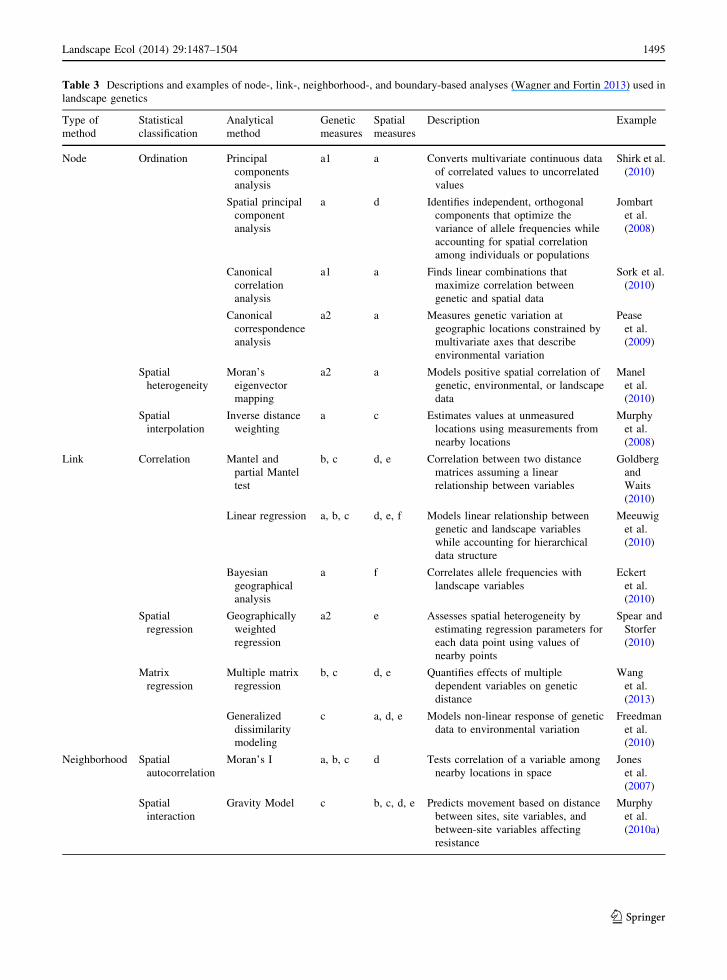
Table 3 Descriptions and examples of node-, link-, neighborhood-, and boundary-based analyses (Wagner and Fortin 2013) used in

landscape genetics

Type of

method

Statistical

classification

Analytical

method

Genetic

measures

Spatial

measures

Description Example

Node Ordination Principal

components

analysis

a1 a Converts multivariate continuous data

of correlated values to uncorrelated

values

Shirk et al.

(2010)

Spatial principal

component

analysis

a d Identifies independent, orthogonal

components that optimize the

variance of allele frequencies while

accounting for spatial correlation

among individuals or populations

Jombart

et al.

(2008)

Canonical

correlation

analysis

a1 a Finds linear combinations that

maximize correlation between

genetic and spatial data

Sork et al.

(2010)

Canonical

correspondence

analysis

a2 a Measures genetic variation at

geographic locations constrained by

multivariate axes that describe

environmental variation

Pease

et al.

(2009)

Spatial

heterogeneity

Moran’s

eigenvector

mapping

a2 a Models positive spatial correlation of

genetic, environmental, or landscape

data

Manel

et al.

(2010)

Spatial

interpolation

Inverse distance

weighting

a c Estimates values at unmeasured

locations using measurements from

nearby locations

Murphy

et al.

(2008)

Link Correlation Mantel and

partial Mantel

test

b, c d, e Correlation between two distance

matrices assuming a linear

relationship between variables

Goldberg

and

Waits

(2010)

Linear regression a, b, c d, e, f Models linear relationship between

genetic and landscape variables

while accounting for hierarchical

data structure

Meeuwig

et al.

(2010)

Bayesian

geographical

analysis

a f Correlates allele frequencies with

landscape variables

Eckert

et al.

(2010)

Spatial

regression

Geographically

weighted

regression

a2 e Assesses spatial heterogeneity by

estimating regression parameters for

each data point using values of

nearby points

Spear and

Storfer

(2010)

Matrix

regression

Multiple matrix

regression

b, c d, e Quantifies effects of multiple

dependent variables on genetic

distance

Wang

et al.

(2013)

Generalized

dissimilarity

modeling

c a, d, e Models non-linear response of genetic

data to environmental variation

Freedman

et al.

(2010)

Neighborhood Spatial

autocorrelation

Moran’s I a, b, c d Tests correlation of a variable among

nearby locations in space

Jones

et al.

(2007)

Spatial

interaction

Gravity Model c b, c, d, e Predicts movement based on distance

between sites, site variables, and

between-site variables affecting

resistance

Murphy

et al.

(2010a)

Landscape Ecol (2014) 29:1487–1504 1495

123

data can be used in node-, link-, neighborhood-, and

boundary-based analyses, whereas landscape or habitat

maps serve as inputs for neighborhood-based analyses

(Table 3). Spatial distance measures, including Euclid-

ean distance and transect or resistance-surface distances,

are useful for link- and neighborhood-based analyses

(Table 3).

Multi- or univariate landscape or environmental

data often need no prior analysis before the final

analysis, but for some analytical methods it may be

necessary to alter spatial input data. Methods such as

PCA and canonical correspondence analysis can be

used to summarize variation in spatial data by

reducing the dimensionality of multivariate data to a

few, independent orthogonal components (Table 3).

Other methods, like inverse distance weighting, are

useful for creating maps of spatial variation from

univariate landscape or environmental data (Table 3).

Landscape or habitat maps are useful input data for

neighborhood-based analyses (Table 3) that relate

genetic diversity or differentiation of sampling locations

to landscape or habitat characteristics surrounding the

locations. Many spatial pattern analyses are available in

packages like FRAGSTATS (McGarigal et al. 2012)

and PATCH ANALYST (Elkie et al. 1999). They can be

used to quantify landscape characteristics and habitat

area or fragmentation of a single patch or of a

neighborhood surrounding a patch. Habitat fragmenta-

tion can also be quantified using o-ring statistics

(Bruggeman et al. 2010).

Spatial input data for link and neighborhood-based

analyses (Table 3) can be generated using network

models that connect sampling locations on a landscape

and estimate distance among locations using informa-

tion about an organism’s movements. Euclidean dis-

tance—the straight-line distance between two

locations—is the simplest distance measure. However,

gene flow often occurs via more complex routes on the

landscape. Transect or resistance-surface distance mea-

sures attempt to account for this complexity by

incorporating landscape or environmental characteris-

tics that may affect gene flow.

Table 3 continued

Type of

method

Statistical

classification

Analytical

method

Genetic

measures

Spatial

measures

Description Example

Boundary Edge

detection

Monmonier’s

algorithm

a2 b, c Finds edges with highest rate of change Manni

et al.

(2004)

Wombling a2 b, c Detects areas of abrupt change on allele

frequency surfaces or maps of landscape or

environmental variables

Cercueil

et al.

(2007)

Spatial

Bayesian

clustering

Boundary detection

(GENELAND;

Guillot et al.

2005)

a1 d Estimates number of genetic populations by

maximizing Hardy–Weinberg and linkage

equilibria; defines boundaries given prior

information about the number of

populations

Heidinger

et al.

(2013)

Local spatial

dependence

(TESS; Chen

et al. 2007)

a1 d Estimates number of genetic populations by

maximizing Hardy–Weinberg and linkage

equilibria; defines clusters by minimizing

heterozygosity reduction caused by

population sub-structure and local spatial

dependence

Rico et al.

(2014)

Spatial

overlap

Boundary overlap d g Quantifies spatial overlap of boundary

locations for genetic populations and

landscape or environmental characteristics

Blair et al.

(2012)

The type of genetic and spatial input data varies among methods

Genetic input data (a) descriptive: 1, genotypes; 2, allele frequencies, (b) migration, (c) distance, (d) output from boundary-based

analysis

Spatial input data (a) multivariate landscape or environmental data, (b) landscape or habitat maps, (c) univariate landscape or

environmental data, (d) geographic coordinates or Euclidean distance, (e) transect or resistance-surface distance, (f) output from

node-based analysis of landscape or environmental data, (g) output from boundary-based analysis

1496 Landscape Ecol (2014) 29:1487–1504

123

Table 4 Characteristics of population- and individual-based genetic measures including descriptive (basic statistics describing

genetic variation), migration (migration rate or number of migrants), and distance (genetic differentiation) measures

Type of

measure

Data type Genetic measure Parameter Key characteristics Citation

Population Descriptive Heterozygosity He Commonly used measure of variation Beebee and

Rowe (2008)

Percentage of

polymorphism

%P Simple measure of variation used with

allozymes or AFLPs

Beebee and

Rowe (2008)

Allele frequency p Simple measure of variation Beebee and

Rowe (2008)

Allelic richness A Simple measure of variation; more

sensitive to founder effects than

heterozygosity

Beebee and

Rowe (2008)

Migration Migration rate M Migration rate over longer time scales

from MIGRATE; assumes mutation-

drift equilibrium

Beerli and

Felsenstein

(2001)

Migration rate m Migration rate over shorter time scales

from BAYESASS

Wilson and

Rannala

(2003)

No. of migrants Nm Number of migrants over longer time

scales from MIGRATE; assumes

mutation-drift equilibrium

Beerli and

Felsenstein

(2001)

Distance F-statistic FST or

FST/(1 - FST)

Common measure of differentiation

among populations; assumes

mutation-drfit equilibrium

Wright (1931),

Rousset

(1997)

F-statistic

analogue

RST Measures differentiation among

populations using msats; assumes

marker follows a stepwise mutation

model

Slatkin (1995)

F-statistic

analogue

h Require no assumptions about number

of populations sampled, sample size,

or heterozygosity of loci; assumes

mutation-drift equilibrium

Weir and

Cockerham

(1984)

Jost’s D DJ Measures fraction of allelic variation

among populations

Jost (2008)

Standardized

distance

G’ST Standardized measure that divides

population differentiation by the

maximum possible

differentiation; assumes mutation-

drift equilibrium

Hedrick

(2005)

Chord distance DC Assumes gene frequency distribution is

Gaussian; more robust when variance

of gene frequencies is small; depends

on number of low-frequency alleles;

assumes mutation-drift equilibrium

Cavalli-Sforza

and Edwards

(1967)

Chord distance DA Less dependent on number of low-

frequency alleles than Dc; assumes

mutation-drift equilibrium

Nei et al

(1983)

Standard distance DS Assumes no migration and a mutation-

drift equilibrium; can be applied to

organisms with different ploidys and

mating schemes

Nei (1972)

Landscape Ecol (2014) 29:1487–1504 1497

123

Transects quantify proportions of different land-

scape or environmental characteristics along straight

lines among sampled locations in a network. Transect

width should be selected to match the spatial scale at

which the study organism interacts with the landscape.

Some studies have used multiple strip widths to test

the effect of landscape or environmental characteris-

tics on gene flow at different spatial scales (Emaresi

et al. 2009; Murphy et al. 2010b).

Resistance surfaces are raster-based maps of land-

scape or environmental characteristics that model

permeability of different habitat types to dispersal

(Spear et al. 2010; Zeller et al. 2012). Each cell on a

resistance surface is assigned a cost value, with high

costs given to habitats that restrict dispersal and low

costs to those that facilitate dispersal. Cost values can

be assigned using expert opinion, habitat suitability

estimated from presence/absence data, movement data

from tagging and tracking studies, or genetic data

(Spear et al. 2010; Zeller et al. 2012). With genetic

data, cost values are assigned using optimization

methods to identify parameter values for landscape or

environmental characteristics that maximize the cor-

relation of genetic distance with resistance-surface

distance (Shirk et al. 2010; Graves et al. 2013).

Distance among sampling locations on a resistance

surface is measured using one or more least-cost paths.

A least-cost path is a predicted rectilinear path for an

organism that minimizes the cost of dispersal between

two locations (Spear et al. 2010). Resistance surfaces

can be used to estimate least-cost distance (e.g. Epps

et al. 2007), resistance distance (e.g. McRae 2006), or

a least-cost transect (e.g. Van Strien et al. 2012).

Least-cost distance (total cost of a least-cost path)

Table 4 continued

Type of

measure

Data type Genetic measure Parameter Key characteristics Citation

Conditional graph

distance

cGD Uses differences in covariation

associated with direct and indirect

gene flow; does not assume a

hierarchical framework of

populations; does not use averaging

statistics or coalescence; distance

matrix produced is equivalent to an

AMOVA matrix

Dyer and

Nason

(2004)

Individual Descriptive Genotype pq Set of alleles possessed by an

individual

Beebee and

Rowe (2008)

Distance Jaccard

coefficient

J Used with AFLPs; unaffected by

homoplasic absent bands

Jaccard (1908)

Dice coefficient D Used with AFLPs; gives weight to

bands present in both individuals

Dice (1945)

Simple-matching

coefficient

M Used with AFLPs; double-band

absence and presence contribute

equally; can be used in AMOVA

Sokal and

Michener

(1958)

Proportion of

shared alleles

PS (DPS) Easy to calculate Bowcock et al.

(1994)

Bray-Curtis

percentage

dissimilarity

d Accounts for semi-quantitative nature

of 3-state genetic data; double

negatives are not counted; abundant

and rare alleles contribute equally to

distance

Bray and

Curtis (1957)

Rousset’s a ar Asymptotically unbiased, except for

small sample sizes; based on

isolation by distance in continuously

distributed species

Rousset

(2000)

PCA-based

genetic distance

DPCA Gives more weight to loci with greater

variation

Shirk et al.

(2010)

1498 Landscape Ecol (2014) 29:1487–1504

123

can be easily calculated from resistance surfaces, but

it assumes organisms make movement decisions with

perfect knowledge of their environment and, there-

fore, may not capture the true range of dispersal routes

across a landscape (Spear et al. 2010). Resistance

distance (the average length of several least-cost

paths) accounts for different dispersal routes across a

landscape (McRae 2006), but, unlike transect meth-

ods, does not account for characteristics of the

landscape surrounding the least-cost paths. The

least-cost transect method is a hybrid of transect and

resistance surface methods. It calculates distances

among habitat patches on a resistance surface using a

least-cost model, but also incorporates a proportion of

the landscape or environmental characteristics sur-

rounding the path within a specified transect width

(Van Strien et al. 2012). This method may be useful for

modeling movements of larger organisms that interact

with the environment at larger spatial scales, or for

organisms that disperse more slowly and may require

wider dispersal corridors to accommodate movement

among patches over longer time periods.

Step 7: choose an analytical method that integrates

genetic and spatial data

The final step in a landscape genetics study is to

integrate genetic and spatial data (Fig. 1, Step 7) in a

multiple-hypothesis testing framework using analyti-

cal methods to achieve the study objectives (Table 1).

Four types of analytical methods can be used: node-,

link-, neighborhood-, and boundary-based methods

(Wagner and Fortin 2013).

Node-based analyses integrate genetic and spatial

data at sampling locations, and some, including inverse

distance weighting, Moran’s eigenvector mapping, and

PCA (Table 3), can be used to convert genetic or spatial

data into inputs for the final analysis. Inverse distance

weighting visualizes genetic variation as a continuous

‘‘genetic surface’’ (Murphy et al. 2008) that can serve as

an input for link- or neighborhood-based analyses.

Moran’s eigenvector mapping measures positive spatial

correlation between geographic locations and genetic,

environmental, or landscape data. It was used to

incorporate the effects of unmeasured environmental

variation in a study of adaptive genetic variation of an

alpine plant (Arabis alpina; Manel et al. 2010). Also,

PCA can be used to reduce the dimensionality of

multilocus genotypes or environmental data.

Node-based analyses also describe spatial patterns

of genetic data to understand gene flow or selection

(Table 1). Spatial principal components analysis

identifies independent, orthogonal components that

optimize the variance of allele frequencies while

accounting for spatial correlation of individuals or

populations (Table 3). This method can be used to

identify global and local patterns of genetic variation

(Jombart et al. 2008). Other ordination methods,

including canonical correlation analysis and canonical

correspondence analysis, have been used to under-

stand patterns of selection. Canonical correlation

analysis identifies linear combinations that maximize

the correlation between genetic and spatial data,

whereas canonical correspondence analysis measures

variation in a dependent variable at geographic

locations constrained by multivariate axes that

describe environmental variation at those locations.

Link-based analyses, such as Mantel or partial

Mantel tests, relate pair-wise measures of genetic

differentiation to geographic distance measures to

identify landscape or environmental characteristics

that restrict or enhance gene flow. Mantel or partial

Mantel tests are the most commonly used analytical

methods in landscape genetics (Storfer et al. 2010;

Table 3). They examine the correlation between a

matrix of pair-wise genetic distances and a matrix of

spatial distances (see Diniz-Filho et al. 2013 for

review). Despite their frequent use, Mantel tests have

been criticized for having low power and inflated type

I error rates (Legendre and Fortin 2010). Cushman

et al. (2013a) observed elevated type I error rates

caused by high correlation among different resistance

models. In spite of these shortcomings, Mantel tests

have very low type II error rates (Cushman et al.

2013a) and, when applied and interpreted correctly,

can be useful for understanding spatial patterns of

genetic differentiation (Diniz-Filho et al. 2013).

Other link-based analyses, including linear regres-

sion, Bayesian geographic analysis (BGA), multiple

matrix regression, and generalized dissimilarity mod-

eling (GDM), have been used to identify landscape or

environmental characteristics that affect gene flow

(Table 3). Linear regression models the linear rela-

tionship between genetic and spatial data while

accounting for hierarchical data structure. In contrast,

when the response of genetic data to the landscape is

non-linear, GDM can be used (e.g. Freedman et al.

2010). Multiple matrix regression was used by

Landscape Ecol (2014) 29:1487–1504 1499

123

Wang et al. (2013) to quantify the contributions of

both landscape and environmental characteristics to

gene flow. This method is especially useful for conser-

vation and management efforts because it can be used to

disentangle the effects of gene flow and selection across

a landscape and identify regions of local adaptation.

Finally, while most analytical methods employ frequ-

entist statistical approaches, BGA examines the asso-

ciation of different loci with environmental variables to

infer selection (Eckert et al. 2010).

Neighborhood-based analyses are useful for under-

standing demographic and metapopulation processes or

measuring spatial autocorrelation, because they inte-

grate genetic data with characteristics of the landscape

surrounding sampling locations. Moran’s I can be used

to estimate the scale of gene flow by measuring spatial

autocorrelation, and gravity models assess demographic

and metapopulation processes (Table 3). Similar to

node-based analyses, they measure characteristics of

sampling locations, such as habitat area or population

growth, but in addition, they incorporate landscape or

environmental characteristics along transects among

sampling locations (Table 3). For example, Murphy

et al. (2010a) used a gravity model to assess connec-

tivity among montane lakes in a metapopulation of

Columbia spotted frogs (Rana luteiventris).

Boundary-based analyses identify dispersal barriers

by measuring spatial overlap of genetic and landscape

or environmental discontinuities on the landscape. In a

spatial context, boundaries identify regions of change

in landscape or environmental characteristics such as

habitat type or precipitation. They can be measured

with edge detection techniques, including Monmo-

nier’s algorithm (1973) and wombling (Womble 1951;

Table 3). In a genetic context, boundaries act as

barriers to gene flow, separating panmictic popula-

tions. Genetic boundaries can be identified using edge

detection techniques, Bayesian clustering methods

implemented in programs such as GENELAND

(Guillot et al. 2005) or TESS (Chen et al. 2007;

Table 3), or non-Bayesian clustering methods includ-

ing PSMIX (Wu et al. 2006) and discriminant analysis

of principle components (Jombart et al. 2010). Statis-

tical power of edge detection and clustering methods

to detect a genetic barrier in simulated data sets with

different conditions for dispersal and genetic equilib-

rium has been compared by Blair et al. (2012). Their

results indicated that clustering methods outperformed

edge detection methods, that barriers can be detected

more rapidly in species with long distance dispersal,

and that isolation by distance can confound the

identification of barriers using these methods. The

coincidence of boundaries can be determined by

overlaying maps of landscape or environmental char-

acteristics and genetic population clusters. Statistical

methods to assess boundary overlap have been devel-

oped (Jacquez 1995), but have been underutilized in

landscape genetics.

Finally, it is important to consider the framework

that will be used for testing multiple hypotheses or

selecting among models to ensure accurate inference

from statistical methods and to minimize the influence

of spurious correlations on the interpretation of

landscape genetics patterns. Cushman et al. (2006)

introduced a causal modeling approach to test com-

peting hypotheses using partial Mantel tests. Improve-

ments to the approach have been made by Shirk et al.

(2010), and Cushman et al. (2013a, b). Others have

used Akaike’s information criterion (Burnham and

Anderson 2002) to compare candidate models using

linear modeling (Meeuwig et al. 2010) and gravity

modeling (Murphy et al. 2010a). In addition to

frequentist methods, Bayesian geographical analyses

have used Bayes factors as measures of support for

relationships between candidate landscape or environ-

mental variables and genetic data (Eckert et al. 2010).

Concluding remarks

A successful landscape genetics study combines

genetic and landscape or environmental data to make

spatially-explicit conclusions about factors affecting

gene flow or selection. The projection of landscape

genetics patterns to larger spatial and temporal scales

through simulations is a valuable tool for management

(e.g. Wasserman et al. 2012) and will likely influence

future conservation decisions and mitigation efforts,

especially as habitat loss and fragmentation and

climate change alter landscapes. Emerging technolo-

gies, such as high throughput sequencing, advances in

remote sensing, and low-cost climate data loggers,

have and will continue to facilitate the collection and

analysis of genetic, landscape, and environmental data

at greater resolutions and finer scales. The resulting

abundance of data allows researchers to explore

patterns, and the processes that generate them, with

increased statistical power (Schwartz et al. 2010;

1500 Landscape Ecol (2014) 29:1487–1504

123

Schoville et al. 2012). Future progress in theory and

application of landscape genetics depends upon

hypothesis-driven research that utilizes empirical data

from controlled, replicated experiments to test

observed patterns, and uses simulation modeling to

understand how relationships between patterns and

processes change across spatial and temporal scales

(Cushman 2014). As genetic and spatial data sets

increase in size, complexity, and resolution, new study

design considerations and analytical methods will

surely arise. The landscape genetics framework pre-

sented here (Fig. 1) can accommodate new design

considerations and analyses, and facilitate integration

of genetic and spatial data by guiding new landscape

geneticists through study design, implementation, and

analysis.

Acknowledgments We thank the Beissinger Lab for

discussions and advice during development of this manuscript.

Constructive comments were also provided by N. VanSchmidt,

K. Iknayan, J. Belton, two anonymous reviewers, and the

associate editor. Financial support was provided by the National

Science Foundation DEB-1051342 and CNH 1115069 to SRB.

References

Amos JN, Bennett AF, Mac Nally R, Newell G, Pavlova, A,

Radford JQ, Thomson JR, White M, Sunnucks P (2012)

Predicting landscape-genetic consequences of habitat loss,

fragmentation and mobility for multiple species of wood-

land birds. PLoS ONE 7:e30888

Anderson CD, Epperson BK, Fortin MJ, Holderegger R, James

P, Rosenberg MS, Scribner K, Spear S (2010) Considering

spatial and temporal scale in landscape-genetic studies of

gene flow. Mol Ecol 19:3565–3575

Balkenhol N, Gugerli F, Cushman SA, Waits LP, Coulon A,

Arntzen JW, Holderegger R, Wagner HH, Participants of

the Landscape Genetics Research Agenda Workshop 2007

(2009a) Identifying future research needs in landscape

genetics: where to from here? Landscape Ecol 24:455–463

Balkenhol N, Waits LP, Dezzani RJ (2009b) Statistical

approaches in landscape genetics: an evaluation of meth-

ods for linking landscape and genetic data. Ecography

32:818–830

Beebee T, Rowe G (2008) An introduction to molecular ecol-

ogy, 2nd edn. Oxford University Press, New York

Beerli P, Felsenstein J (2001) Maximum likelihood estimation

of a migration matrix and effective population sizes in n

subpopulations by using a coalescent approach. Proc Natl

Acad Sci 98:4563–4568

Blair C, Weigel DE, Balazik M, Keeley ATH, Walker FM,

Landguth E, Cushman S, Murphy M, Waits L, Balkenhol N

(2012) A simulation-based evaluation of methods for

inferring linear barriers to gene flow. Mol Ecol Resour

12:822–833

Bowcock AM, Ruiz-Linares A, Tomfohrde J, Minch E, Kidd JR,

Cavalli-Sforza LL (1994) High resolution of human trees

with polymorphic microsatellites. Nature 368:455–457

Bradburd GS, Ralph PL, Coop GM (2013) Disentangling the

effects of geographic and ecological isolation on genetic

differentiation. Evolution 67:3258–3273

Bray JR, Curtis JT (1957) An ordination of the upland forest

communities of southern Wisconsin. Ecoloical Monogr

27:325–349

Bruggeman DJ, Wiegand T, FernaNdez N (2010) The relative

effects of habitat loss and fragmentation on population

genetic variation in the red-cockaded woodpecker (Pico-

ides borealis). Mol Ecol 19:3679–3691

Burnham KP, Anderson DR (2002) Model selection and mul-

timodel inference: a practical information-theoretic

approach, 2nd edn. Springer, New York

Castillo JA, Epps CW, Davis AR, Cushman SA (2014) Land-

scape effects on gene flow for a climate-sensitive montane

species, the American pika. Mol Ecol 23:843–856

Cavalli-Sforza LL, Edwards AW (1967) Phylogenetic analysis.

Models and estimation procedures. Am J Hum Genet 19:233

Cercueil A, Francois O, Manel S (2007) The genetical band-

width mapping: a spatial and graphical representation of

population genetic structure based on the Wombling

method. Theor Popul Biol 71:332–341

Chen C, Durand E, Forbes F, FrancOis O (2007) Bayesian

clustering algorithms ascertaining spatial population

structure: a new computer program and a comparison

study. Mol Ecol Notes 7:747–756

Cushman SA (2014) Grand challenges in evolutionary and

population genetics: the importance of integrating epige-

netics, genomics, modeling, and experimentation. Front

Genet 5:197

Cushman SA, Landguth EL (2010a) Spurious correlations and

inference in landscape genetics. Mol Ecol 19:3592–3602

Cushman SA, Landguth EL (2010b) Scale dependent inference

in landscape genetics. Landscape Ecol 25:967–979

Cushman SA, McKelvey KS, Hayden J, Schwartz MK (2006)

Gene flow in complex landscapes: testing multiple

hypotheses with causal modeling. Am Nat 168:486–499

Cushman SA, Shirk A, Landguth EL (2011) Separating the

effects of habitat area, fragmentation and matrix resistance

on genetic differentiation in complex landscapes. Land-

scape Ecol 27:369–380

Cushman S, Wasserman T, Landguth E, Shirk A (2013a) Re-

evaluating causal modeling with Mantel tests in landscape

genetics. Diversity 5:51–72

Cushman SA, Max TL, Whitham TG, Allan GJ (2013b) River

network connectivity and climate gradients drive genetic

differentiation in a riparian foundation tree. Ecol Appl

24:1000–1014

Dice LR (1945) Measures of the amount of ecologic association

between species. Ecology 26:297–302

Diniz-Filho JAF, Soares TN, Lima JS, Dobrovolski R, Landeiro

VL, de C Telles MP, Rangel TF, Bini LM (2013) Mantel

test in population genetics. Genet Mol Biol 36:475–485

Dobzhansky T (1947) A directional change in the genetic con-

stitution of a natural population of Drosophila pseud-

oobscura. Heredity 1:53–64

Dyer RJ, Nason JD (2004) Population Graphs: the graph theo-

retic shape of genetic structure. Mol Ecol 13:1713–1727

Landscape Ecol (2014) 29:1487–1504 1501

123

Eckert AJ, Bower AD, GonzaLez-MartıNez SC, Wegrzyn JL,

Coop G, Neale DB (2010) Back to nature: ecological

genomics of loblolly pine (Pinus taeda, Pinaceae). Mol

Ecol 19:3789–3805

Elkie PC, Rempel RS, Carr A, et al. (1999) Patch analyst user’s

manual: a tool for quantifying landscape structure. Ontario

Ministry of Natural Resources, Boreal Science, Northwest

Science & Technology, Thunder Bay

Elliot NB, Cushman SA, Macdonald DW, Loveridge AJ (2014)

The devil is in the dispersers: predictions of landscape

connectivity change with demography. J Appl Ecol. doi:10.

1111/1365-2664.12282

Emaresi G, Pellet J, Dubey S et al (2009) Landscape genetics of

the Alpine newt (Mesotriton alpestris) inferred from a

strip-based approach. Conserv Genet 12:41–50

Epperson BK, Chung MG (2001) Spatial genetic structure of

allozyme polymorphisms within populations of Pinus

strobus (Pinaceae). Am J Bot 88:1006–1010

Epperson BK, Mcrae BH, Scribner K, Cushman SA, Rosenberg

MS, Fortin M-J, James PMA, Murphy M, Manel S,

Legendre P, Dale MRT (2010) Utility of computer simu-

lations in landscape genetics. Mol Ecol 19:3549–3564

Epps CW, Wehausen JD, Bleich VC, Torres SG, Brashares JS

(2007) Optimizing dispersal and corridor models using

landscape genetics. J Appl Ecol 44:714–724

Freedman AH, Thomassen HA, Buermann W, Smith TB (2010)

Genomic signals of diversification along ecological gra-

dients in a tropical lizard. Mol Ecol 19:3773–3788

Galpern P, Manseau M (2013) Finding the functional grain:

comparing methods for scaling resistance surfaces. Land-

scape Ecol 28:1269–1281

Girard P, Takekawa JY, Beissinger SR (2010) Uncloaking a

cryptic, threatened rail with molecular markers: origins,

connectivity and demography of a recently-discovered

population. Conserv Genet 11:2409–2418

Goldberg CS, Waits LP (2010) Comparative landscape genetics

of two pond-breeding amphibian species in a highly

modified agricultural landscape. Mol Ecol 19:3650–3663

Graves TA, Beier P, Royle JA (2013) Current approaches using

genetic distances produce poor estimates of landscape resis-

tance to interindividual dispersal. Mol Ecol 22:3888–3903

Guillot G, Mortier F, Estoup A (2005) Geneland: a computer

package for landscape genetics. Mol Ecol Notes 5:712–715

Hale ML, Burg TM, Steeves TE (2012) Sampling for micro-

satellite-based population genetic studies: 25–30 individ-

uals per population is enough to accurately estimate allele

frequencies. PLoS ONE 7:e45170

He Q, Edwards DL, Knowles LL (2013) Integrative testing of how

environments from the past to the present shape genetic

structure across landscapes. Evolution 67:3386–3402

Hedrick PW (1999) Perspective: highly variable loci and their

interpretation in evolution and conservation. Evolution

53:313

Hedrick PW (2005) A standardized genetic differentiation

measure. Evolution 59:1633–1638

Heidinger IMM, Hein S, Feldhaar H, Poethke H-J (2013) The

genetic structure of populations of Metrioptera bicolor in a

spatially structured landscape: effects of dispersal barriers

and geographic distance. Conserv Genet 14:299–311

Holderegger R, Wagner HH (2006) A brief guide to Landscape

Genetics. Landscape Ecol 21:793–796

Holderegger R, Wagner HH (2008) Landscape genetics. Bio-

science 58:199–207

Holderegger R, Kamm U, Gugerli F (2006) Adaptive versus

neutral genetic diversity: implications for landscape

genetics. Landscape Ecol 21:797–807

Holzhauer SIJ, Wolff K, Wolters V (2009) Changes in land use

and habitat availability affect the population genetic

structure of Metrioptera roeselii (Orthoptera: Tettigonii-

dae). J Insect Conserv 13:543–552

Jaccard P (1908) Nouvelles recherches sur la distribution florale.

Bull Soc Vaudoise Sci Nat 44:223–270

Jacquez GM (1995) The map comparison problem: tests for the

overlap of geographic boundaries. Stat Med 14:2343–2361

Jombart T, Devillard S, Dufour AB, Pontier D (2008) Revealing

cryptic spatial patterns in genetic variability by a new

multivariate method. Heredity 101:92–103

Jombart T, Devillard S, Balloux F (2010) Discriminant analysis

of principal components: a new method for the analysis of

genetically structured populations. BMC Genet 11:94

Jones TH, Vaillancourt RE, Potts BM (2007) Detection and

visualization of spatial genetic structure in continuous

Eucalyptus globulus forest. Mol Ecol 16:697–707

Jost L (2008) GST and its relatives do not measure differentia-

tion. Mol Ecol 17:4015–4026

Kalinowski ST (2002) Evolutionary and statistical properties of

three genetic distances. Mol Ecol 11:1263–1273

Kimura M (1969) The number of heterozygous nucleotide sites

maintained in a finite population due to steady flux of

mutations. Genetics 61:893

Kimura M, Ohta T (1978) Stepwise mutation model and dis-

tribution of allelic frequencies in a finite population. Proc

Natl Acad Sci 75:2868–2872

Koen EL, Bowman J, Garroway CJ, Wilson PJ (2013) The

sensitivity of genetic connectivity measures to unsampled

and under-sampled sites. PLoS ONE 8:e56204

Landguth EL, Cushman SA (2010) CDPOP: a spatially explicit

cost distance population genetics program. Mol Ecol Re-

sour 10:156–161

Landguth EL, Cushman SA, Schwartz MK, McKelvey KS,

Murphy M, Luikart G (2010) Quantifying the lag time to

detect barriers in landscape genetics. Mol Ecol 19:4179–4191

Landguth EL, Cushman SA, Johnson NA (2012a) Simulating

natural selection in landscape genetics. Mol Ecol Resour

12:363–368

Landguth EL, Fedy BC, Oyler-McCance SJ, Garey AL, Emel

SL, Mumma M, Wagner HH, Fortin M-J, Cushman SA.

(2012b) Effects of sample size, number of markers, and

allelic richness on the detection of spatial genetic pattern.

Mol Ecol Resour 12:276–284

Latta RG (2006) Integrating patterns across multiple genetic

markers to infer spatial processes. Landscape Ecol

21:809–820

Legendre P, Fortin M-J (2010) Comparison of the Mantel test

and alternative approaches for detecting complex multi-

variate relationships in the spatial analysis of genetic data.

Mol Ecol Resour 10:831–844

Manel S, Holderegger R (2013) Ten years of landscape genetics.

Trends Ecol Evol 28:614–621

Manel S, Schwartz MK, Luikart G, Taberlet P (2003) Landscape

genetics: combining landscape ecology and population

genetics. Trends Ecol Evol 18:189–197

1502 Landscape Ecol (2014) 29:1487–1504

123

Manel S, Poncet BN, Legendre P, Gugerli F, Holderegger R

(2010) Common factors drive adaptive genetic variation at

different spatial scales in Arabis alpina. Mol Ecol

19:3824–3835

Manel S, Albert C, Yoccoz N (2012) Sampling in landscape

genomics. In: Pompanon F, Bonin A (eds) Data Prod.

Humana Press, Anal Popul Genomics, pp 3–12

Manni F, Guerard E, Heyer E (2004) Geographic patterns of

(genetic, morphologic, linguistic) variation: how barriers

can be detected by using Monmonier’s algorithm. Hum

Biol 76:173–190

McGarigal K, Cushman S, Ene E (2012) FRAGSTATS v4:

spatial pattern analysis program for categorical and con-

tinuous maps. University of Massachusetts, Amherst

McRae BH (2006) Isolation by resistance. Evolution 60:1551–1561

Meeuwig MH, Guy CS, Kalinowski ST, Fredenberg WA (2010)

Landscape influences on genetic differentiation among bull

trout populations in a stream-lake network. Mol Ecol

19:3620–3633

Monmonier MS (1973) Maximum-difference barriers: an

alternative numerical regionalization method. Geogr Anal

5:245–261

Murphy MA, Evans JS, Cushman SA, Storfer A (2008) Repre-

senting genetic variation as continuous surfaces: an

approach for identifying spatial dependency in landscape

genetic studies. Ecography 31:685–697

Murphy MA, Dezzani R, Pilliod DS, Storfer A (2010a) Land-

scape genetics of high mountain frog metapopulations. Mol

Ecol 19:3634–3649

Murphy MA, Evans JS, Storfer A (2010b) Quantifying Bufo

boreas connectivity in Yellowstone National Park with

landscape genetics. Ecology 91:252–261

Nei M (1972) Genetic distance between populations. Am Nat

106:283–292

Nei M, Tajima F, Tateno Y (1983) Accuracy of estimated phy-

logenetic trees from molecular data. J Mol Evol 19:153–170

O’brien RM (2007) A caution regarding rules of thumb for

variance inflation factors. Qual Quant 41:673–690

Oyler-McCance SJ, Fedy BC, Landguth EL (2013) Sample design

effects in landscape genetics. Conserv Genet 14:275–285

Pavlacky DC Jr, Goldizen AW, Prentis PJ, Nicholls JA, Lowe

AJ (2009) A landscape genetics approach for quantifying

the relative influence of historic and contemporary habitat

heterogeneity on the genetic connectivity of a rainforest

bird. Mol Ecol 18:2945–2960

Pease KM, Freedman AH, Pollinger JP, Mccormack JE, Buer-

mann W, Rodzen J, Banks J, Meredith E, Bleich VC,

Schaefer RJ, Jones K, Wayne RK (2009) Landscape

genetics of California mule deer (Odocoileus hemionus):

the roles of ecological and historical factors in generating

differentiation. Mol Ecol 18:1848–1862

Rico Y, Holderegger R, Boehmer HJ, Wagner HH (2014)

Directed dispersal by rotational shepherding supports

landscape genetic connectivity in a calcareous grassland

plant. Mol Ecol 23:832–842

Rousset F (1997) Genetic differentiation and estimation of gene

flow from F-statistics under isolation by distance. Genetics

145:1219–1228

Rousset F (2000) Genetic differentiation between individuals.

J Evol Biol 13:58–62

Saenz-Romero C, Guries RP, Monk AI (2001) Landscape

genetic structure of Pinus banksiana: allozyme variation.

Can J Bot 79:871–878

Schoville SD, Bonin A, Francois O, Lobreaux S, Melodelima C,

Manel S (2012) Adaptive genetic variation on the land-

scape: methods and cases. Annu Rev Ecol Evol Syst

43:23–43

Schwartz MK, McKelvey KS (2008) Why sampling scheme

matters: the effect of sampling scheme on landscape

genetic results. Conserv Genet 10:441–452

Schwartz MK, McKelvey KS, Cushman SA, Luikart G (2010)

Landscape genomics: a brief perspective. In: Cushman SA,

Huettmann F (eds) Spat. complex comprehensive conser-

vation. Springer, Tokyo, pp 165–174

Segelbacher G, Cushman SA, Epperson BK et al (2010)

Applications of landscape genetics in conservation biol-

ogy: concepts and challenges. Conserv Genet 11:375–385

Shirk AJ, Wallin DO, Cushman SA, Rice CG, Warheit KI

(2010) Inferring landscape effects on gene flow: a new

model selection framework. Mol Ecol 19:3603–3619

Shirk AJ, Cushman SA, Landguth EL (2012) Simulating pat-

tern–process relationships to validate landscape genetic

models. Int J Ecol 2012:1–8

Slatkin M (1987) Gene flow and the geographic structure of

natural populations. Science 236:787–792

Slatkin M (1993) Isolation by distance in equilibrium and non-

equilibrium populations. Evolution 47:264–279

Slatkin M (1995) A measure of population subdivision based on

microsatellite allele frequencies. Genetics 139:457–462

Sokal RR, Michener CD (1958) A statistical method for eval-

uating systematic relationships. Univ Kans Sci Bull

38:1409–1438

Sork VL, Davis FW, Westfall R et al (2010) Gene movement

and genetic association with regional climate gradients in

California valley oak (Quercus lobata Nee) in the face of

climate change. Mol Ecol 19:3806–3823

Spear SF, Storfer A (2010) Anthropogenic and natural distur-

bance lead to differing patterns of gene flow in the Rocky

Mountain tailed frog, Ascaphus montanus. Biol Conserv

143:778–786

Spear SF, Balkenhol N, Fortin M-J, Mcrae BH, Scribner K

(2010) Use of resistance surfaces for landscape genetic

studies: considerations for parameterization and analysis.

Mol Ecol 19:3576–3591

Storfer A, Murphy MA, Evans JS, Goldberg CS, Robinson S,

Spear SF, Dezzani R, Delmelle E, Vierling L, Waits LP

(2006) Putting the ‘‘landscape’’ in landscape genetics.

Heredity 98:128–142

Storfer A, Murphy MA, Spear SF et al (2010) Landscape

genetics: where are we now? Mol Ecol 19:3496–3514

Van Strien MJ, Keller D, Holderegger R (2012) A new analyt-

ical approach to landscape genetic modelling: least-cost

transect analysis and linear mixed models. Mol Ecol

21:4010–4023

Wagner HH, Fortin M-J (2013) A conceptual framework for the

spatial analysis of landscape genetic data. Conserv Genet

14:253–261

Wang IJ (2011) Choosing appropriate genetic markers and

analytical methods for testing landscape genetic hypothe-

ses. Mol Ecol 20:2480–2482

Landscape Ecol (2014) 29:1487–1504 1503

123

Wang IJ (2013) Examining the full effects of landscape heter-

ogeneity on spatial genetic variation: a multiple matrix

regression approach for quantifying geographic and eco-

logical isolation. Evolution 67:3403–3411

Wang IJ, Glor RE, Losos JB (2013) Quantifying the roles of

ecology and geography in spatial genetic divergence. Ecol

Lett 16:175–182

Wasserman TN, Cushman SA, Shirk AS, Landguth EL, Littell

JS (2012) Simulating the effects of climate change on

population connectivity of American marten (Martes

americana) in the northern Rocky Mountains, USA.

Landscape Ecol 27:211–225

Weir BS, Cockerham CC (1984) Estimating F-statistics for the

analysis of population structure. Evolution 38:1358–1370

Wilson GA, Rannala B (2003) Bayesian inference of recent

migration rates using multilocus genotypes. Genetics

163:1177

Womble WH (1951) Differential systematics. Science

114:315–322

Wright S (1931) Evolution in Mendelian populations. Genetics

16:97

Wright S (1943) Isolation by distance. Genetics 28:114

Wu B, Liu N, Zhao H (2006) PSMIX: an R package for popu-

lation structure inference via maximum likelihood method.

BMC Bioinf 7:317

Zeller KA, McGarigal K, Whiteley AR (2012) Estimating

landscape resistance to movement: a review. Landsc Ecol

27:777–797

Zellmer AJ, Knowles LL (2009) Disentangling the effects of

historic vs. contemporary landscape structure on popula-

tion genetic divergence. Mol Ecol 18:3593–3602

1504 Landscape Ecol (2014) 29:1487–1504

123