eScholarship provides open access, scholarly publishingservices to the University of California and delivers a dynamicresearch platform to scholars worldwide.

University of California

Peer Reviewed

Title:A Phase-Partitioning Model for CO2–Brine Mixtures at Elevated Temperatures and Pressures:Application to CO2-Enhanced Geothermal Systems

Author:Spycher, Nicolas; Pruess, Karsten

Publication Date:2010

Publication Info:Postprints, Multi-Campus

Permalink:http://escholarship.org/uc/item/0kp5q3vn

DOI:10.1007/s11242-009-9425-y

Abstract:Correlations are presented to compute the mutual solubilities of CO2 and chloride brines attemperatures 12–300°C, pressures 1–600 bar (0.1–60 MPa), and salinities 0–6 m NaCl. Theformulation is computationally efficient and primarily intended for numerical simulations of CO2-water flow in carbon sequestration and geothermal studies. The phase-partitioning model relieson experimental data from literature for phase partitioning between CO2 and NaCl brines, andextends the previously published correlations to higher temperatures. The model relies on activitycoefficients for the H2O-rich (aqueous) phase and fugacity coefficients for the CO2-rich phase.Activity coefficients are treated using a Margules expression for CO2 in pure water, and aPitzer expression for salting-out effects. Fugacity coefficients are computed using a modifiedRedlich–Kwong equation of state and mixing rules that incorporate asymmetric binary interactionparameters. Parameters for the calculation of activity and fugacity coefficients were fitted topublished solubility data over the P–T range of interest. In doing so, mutual solubilities and gas-phase volumetric data are typically reproduced within the scatter of the available data. An exampleof multiphase flow simulation implementing the mutual solubility model is presented for the caseof a hypothetical, enhanced geothermal system where CO2 is used as the heat extraction fluid. Inthis simulation, dry supercritical CO2 at 20°C is injected into a 200°C hot-water reservoir. Resultsshow that the injected CO2 displaces the formation water relatively quickly, but that the producedCO2 contains significant water for long periods of time. The amount of water in the CO2 couldhave implications for reactivity with reservoir rocks and engineered materials.

Transp Porous Med (2010) 82:173–196DOI 10.1007/s11242-009-9425-y

A Phase-Partitioning Model for CO2–Brine Mixturesat Elevated Temperatures and Pressures: Applicationto CO2-Enhanced Geothermal Systems

Nicolas Spycher · Karsten Pruess

Received: 8 December 2008 / Accepted: 1 June 2009 / Published online: 17 July 2009© The Author(s) 2009. This article is published with open access at Springerlink.com

Abstract Correlations are presented to compute the mutual solubilities of CO2 andchloride brines at temperatures 12–300◦C, pressures 1–600 bar (0.1–60 MPa), and salini-ties 0–6 m NaCl. The formulation is computationally efficient and primarily intended fornumerical simulations of CO2-water flow in carbon sequestration and geothermal studies.The phase-partitioning model relies on experimental data from literature for phase parti-tioning between CO2 and NaCl brines, and extends the previously published correlationsto higher temperatures. The model relies on activity coefficients for the H2O-rich (aqueous)phase and fugacity coefficients for the CO2-rich phase. Activity coefficients are treated usinga Margules expression for CO2 in pure water, and a Pitzer expression for salting-out effects.Fugacity coefficients are computed using a modified Redlich–Kwong equation of state andmixing rules that incorporate asymmetric binary interaction parameters. Parameters for thecalculation of activity and fugacity coefficients were fitted to published solubility data overthe P–T range of interest. In doing so, mutual solubilities and gas-phase volumetric dataare typically reproduced within the scatter of the available data. An example of multiphaseflow simulation implementing the mutual solubility model is presented for the case of ahypothetical, enhanced geothermal system where CO2 is used as the heat extraction fluid. Inthis simulation, dry supercritical CO2 at 20◦C is injected into a 200◦C hot-water reservoir.Results show that the injected CO2 displaces the formation water relatively quickly, but thatthe produced CO2 contains significant water for long periods of time. The amount of water inthe CO2 could have implications for reactivity with reservoir rocks and engineered materials.

Keywords CO2 · Carbon dioxide · Solubility · Phase partitioning · Mutual solubility ·Enhanced Geothermal System · EGS · Brine · Water Flow · Multiphase Flow

N. Spycher (B) · K. PruessLawrence Berkeley National Laboratory, MS 90-1116, 1 Cyclotron Road, Berkeley, CA, USAe-mail: NSpycher@lbl.gov

123

174 N. Spycher, K. Pruess

1 Introduction

The burning of fossil fuels has become a serious concern because of associated CO2 emissionsand impacts on climate (IPCC 2005, 2008). As a result, many studies have been undertakento assess the feasibility of CO2 geologic storage as a mitigation measure to curb rising CO2

emissions (IPCC 2005). Rising costs of fossil fuels have also led to a renewed interest ingeothermal energy, and particularly in enhanced geothermal systems (EGS) (MIT 2006).With these systems, the recovery of heat from the subsurface is enhanced by water injection(e.g., Goyal 1995; Stark et al. 2005) and in some cases, water is injected, circulated, andrecovered from areas that originally are dry or contain very little water (e.g., MIT 2006). Theuse of CO2 instead of water as the heat transmission fluid in EGS has been proposed as ameans not only to produce “clean” energy, but also to potentially sequester CO2 through fluidlosses at depth, which typically occur in any type of EGS (Brown 2000; Fouillac et al. 2004;Pruess 2006, 2008). Other potential advantages of CO2-based EGS include increased heatextraction rates and wellbore flow compared to water-based systems, and lesser potential forunfavorable rock–fluid chemical interactions in engineered systems (Pruess 2006, 2008).

The solubility of CO2 in water has obvious implications for long-term carbon sequestra-tion and water–rock interactions (e.g., Gilfillan 2008; Moore et al. 2005; Rosenbauer et al.2005; Palandri et al. 2005; Kaszuba et al. 2003). The solubility of water into CO2 is alsoof importance, because it affects the reactivity of CO2 with surrounding rocks (e.g., Regnaultet al. 2005; Rimmelé et al. 2008; Lin et al. 2008; Suto et al. 2007) and determines the capacityof injected CO2 to dry the rock formations adjacent to injection wells (Giorgis et al. 2007;Hurter et al. 2007; Pruess and Müller 2009). In the case of a CO2-based EGS, the parti-tioning of water into CO2 would also determine the time required for the removal of waterfrom the (central portion of the) EGS, and the type of chemical interactions that may takeplace between the CO2 plume, reservoir rocks, and engineered systems. Therefore, an impor-tant aspect in the study of CO2 geologic storage and CO2–EGS is the calculation of phasepartitioning between CO2 and formation waters.

At temperatures and pressures typically considered for geologic storage (<100◦C and200–400 bar), the mixing of CO2 with water results in two immiscible phases, an H2O-rich liquid phase and a CO2-rich compressed “gas” phase (supercritical fluid) that containsonly small amounts of water (typically < 2 mol%; e.g., Spycher et al. 2003). At higher tem-peratures relevant to CO2-based EGS, the same two-phase behavior persists, although theamount of water in the CO2-rich phase increases significantly, reaching values of up to about40–50 mol% at temperatures ∼275◦C and pressures between 200 and 600 bar (Takenouchiand Kennedy 1964, Todheide and Frank, 1964; Blencoe et al. 2001). At 300◦C, water andCO2 eventually become fully miscible at pressures above ∼567 bar (Blencoe et al. 2001).The ability to compute this phase-partitioning behavior in a reliable and efficient manner iscritical to predicting the flow of water and CO2 in the subsurface using numerical models.

Several models have been proposed to compute the aqueous solubility of CO2, with orwithout consideration of the water solubility in the CO2 phase (see reviews by Hu et al.2007; Spycher et al. 2003; Spycher and Pruess 2005 and references therein). However, mostof these models are either too computationally intensive for their incorporation into efficientmultiphase flow simulators, or consider only the solubility of CO2 in water. We have pre-viously developed a computationally efficient model to calculate the mutual solubilities ofCO2 and water from 12 to 100◦C and up to 600 bar (Spycher et al. 2003). This model waslater extended to chloride brines up to ∼6 m NaCl over the same range of temperatures andpressures (Spycher and Pruess 2005). Here, motivated by the potential for CO2–EGS and

123

Application to CO2-Enhanced Geothermal Systems 175

CO2 geologic storage at temperatures above 100◦C, this mutual solubility model is extendedto temperatures up to 300◦C.

2 Phase-Partitioning Model

2.1 Model Formulation (CO2–H2O System)

Our original model (Spycher et al. 2003) was intended for temperatures ≤100◦C, at whichtwo assumptions held reasonably well when calculating activity and fugacity coefficients:unit activity coefficients for liquid water and aqueous CO2 in pure water, and infinite waterdilution in the compressed CO2 phase. At higher temperatures, these assumptions start to failbecause the mutual solubilities of CO2 and water increase significantly. Therefore, for appli-cations at temperatures >100◦C, an activity coefficient model for liquid water and aqueousCO2 was implemented, and mixing rules for the equation of state were revised as describedbelow. The extended model formulation is such that a smooth transition can be obtained fromthe original model at temperatures ≤100◦C to higher temperatures. The model formulation issummarized below and in Appendices A and B, with parameters listed in Table 1. Additionaldetails can be found in Spycher et al. (2003).

The equilibrium between water and CO2 is expressed by two reactions

H2O(1) <==> H2O(g) KH2O = fH2O(g)/aH2O(1) (1)

CO2(aq) <==> CO2(g) KCO2(g) = fCO2(g)/aCO2(aq) (2)

each with an equilibrium constant K defined in terms of fugacities ( f ) for gaseous H2Oand CO2, and activities (a) for aqueous CO2 and liquid water. Note that the subscript (g)refers to the CO2-rich phase, which for CO2 may be either gaseous, liquid, or supercritical,but for simplicity, will henceforth be referred to as “gas.” Values of K depend only on tem-perature and pressure. The departure from ideality, including concentration effects, is takeninto account by activity coefficients (γ ) for aqueous species and liquid water, and fugacitycoefficients (�) for gaseous species, with the convention that

ai = γi mi (on a molality scale) or ai = γi xi (on a mole-fraction scale) (3)

and

fi = �i pi = �i yi P (4)

where i designates the component in the mixture (CO2 or H2O), m stands for molality,x and y are the mole fractions in the aqueous and compressed gas phases, respectively, p isthe gas partial pressure, and P is the total pressure. By convention, K is expressed using fvalues defined with respect to a reference state fugacity of 1 bar, and with values of a definedon a mole fraction scale for water and a molality scale for aqueous CO2 (e.g., Denbigh1983). Equilibrium constants defined in this way are computed as functions of temperatureand pressure using the following relationships:

K(T,P) = K 0(T,Pref )

exp

((P − Pref )V

RTk

)(5)

with log(K 0)T,Pref and Pref expressed as functions of temperature

F(T ) = a + bT + cT 2 + dT 3 + eT 4 (6)

123

176 N. Spycher, K. Pruess

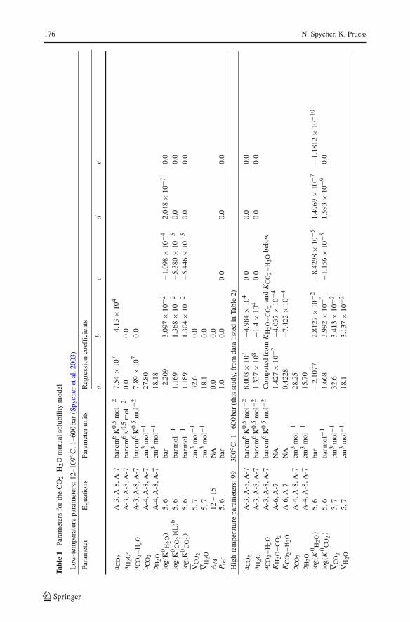
Tabl

e1

Para

met

ers

for

the

CO

2–H

2O

mut

uals

olub

ility

mod

el

Low

-tem

pera

ture

para

met

ers:

12–1

09◦ C

,1–6

00ba

r(S

pych

eret

al.2

003)

Para

met

erE

quat

ions

Para

met

erun

itsR

egre

ssio

nco

effic

ient

s

ab

cd

e

a CO

2A

-3,A

-8,A

-7ba

rcm

6K

0.5

mol

−27.

54×

107

−4.1

3×

104

a H2

Oa

A-3

,A-8

,A-7

barc

m6K

0.5

mol

−20.

00.

0a C

O2−H

2O

A-3

,A-8

,A-7

barc

m6

K0.

5m

ol−2

7.89

×10

70.

0b C

O2

A-4

,A-8

,A-7

cm3

mol

−127

.80

b H2

OA

-4,A

-8,A

-7cm

3m

ol−1

18.1

8lo

g(K

0H

2O

)5,

6ba

r–2

.209

3.09

7×

10−2

−1.0

98×

10−4

2.04

8×

10−7

0.0

log(

K0

CO

2)(

L)b

5,6

barm

ol−1

1.16

91.

368

×10

−2−5

.380

×10

−50.

00.

0lo

g(K

0C

O2)

5,6

barm

ol−1

1.18

91.

304

×10

−2−5

.446

×10

−50.

00.

0� V C

O2

5,7

cm3

mol

−132

.60.

0� V H

2O

5,7

cm3

mol

−118

.10.

0A

M12

–15

NA

0.0

0.0

P ref

5,6

bar

1.0

0.0

0.0

0.0

0.0

Hig

h-te

mpe

ratu

repa

ram

eter

s:99

−30

0◦C

,1−6

00ba

r(t

his

stud

y,fr

omda

talis

ted

inTa

ble

2)

a CO

2A

-3,A

-8,A

-7ba

rcm

6K

0.5

mol

−28.

008

×10

7−4

.984

×10

40.

00.

00.

0a H

2O

A-3

,A-8

,A-7

barc

m6

K0.

5m

ol−2

1.33

7×

108

−1.4

×10

40.

00.

00.

0a C

O2−H

2O

A-3

,A-8

,A-7

barc

m6

K0.

5m

ol−2

Com

pute

dfr

omK

H2

O−C

O2

and

KC

O2−H

2O

belo

wK

H2

O−C

O2

A-6

,A-7

NA

1.42

7×

10−2

−4.0

37×

10−4

KC

O2−H

2O

A-6

,A-7

NA

0.42

28−7

.422

×10

−4b C

O2

A-4

,A-8

,A-7

cm3

mol

−128

.25

b H2

OA

-4,A

-8,A

-7cm

3m

ol−1

15.7

0lo

g(K

0H

2O

)5,

6ba

r−2

.107

72.

8127

×10

−2−8

.429

8×

10−5

1.49

69×

10−7

−1.1

812

×10

−10

log(

K0

CO

2)

5,6

barm

ol−1

1.66

83.

992

×10

−3−1

.156

×10

−51.

593

×10

−90.

0� V C

O2

5,7

cm3

mol

−132

.63.

413

×10

−2� V H

2O

5,7

cm3

mol

−118

.13.

137

×10

−2

123

Application to CO2-Enhanced Geothermal Systems 177

Tabl

e1

cont

inue

d

Para

met

erE

quat

ions

Para

met

erun

itsR

egre

ssio

nco

effic

ient

s

ab

cd

e

AM

12–1

5N

A−3

.084

×10

−21.

927

×10

−5P r

ef(T

≤10

0◦C

)5,

6ba

r1.

00.

00.

00.

00.

0P r

ef(T

>10

0◦C

)c5,

6ba

r−1

.990

6×

10−1

2.04

71×

10−3

1.01

52×

10−4

−1.4

234

×10

−61.

4168

×10

−8C

O2

activ

ityco

effic

ient

for

salt

effe

cts:

∼20

−30

5◦C

(thi

sst

udy,

from

data

liste

din

Tabl

e3)

λ18

,19

NA

2.21

7×

10−4

1.07

426

48ξ

18,1

9N

A1.

30×

10−5

−20.

1252

59

aA

valu

eof

a H2

Ois

notn

eede

dbe

caus

eof

the

assu

mpt

ion

ofy H

2O

=0

inm

ixin

gru

les

bFo

rliq

uid

CO

2be

low

31◦ C

and

abov

eC

O2

satu

ratio

npr

essu

res

cW

ater

satu

ratio

npr

essu

re

123

178 N. Spycher, K. Pruess

and

V = a + b(TK − 373.15) and b = 0 at TK < 373.15 K (7)

where T is the temperature in degrees Celsius, TK is the temperature in degrees Kelvin,P is the total pressure of the system in bar, and Pref is a reference pressure, here takenas 1 bar up to 100◦C, and as the pure water saturation pressure above 100◦C. R is the gasconstant, and V is the average partial molar volume of the pure condensed phase (CO2 orwater) over the pressure interval Pref to P . Coefficients a through e are regression coeffi-cients that can express, as needed, the non-linearity in Gibbs free energy and V changes withtemperature at constant pressure.

The mutual solubilities of water and CO2 are then expressed as follows:

yH2O = A(1 − xCO2) (8)

xCO2 = B(1 − yH2O) (9)

with parameters A and B defined as (using values of K given by Eqs. 5–7)

A = KH2OγH2O

�H2O Ptot(10)

B = �CO2 Ptot

55.508 γCO2 KCO2

(11)

Note that in these expressions, the activity coefficients γH2O and γCO2 are both defined ona mole fraction scale, although KCO2 is still defined on a molality scale. At temperatures≤100◦C and pressures of interest (up to 600 bar), the solubility of CO2 in water is limited,such that a satisfactory accuracy is obtained by assuming γH2O = 1 and γCO2 = 1. At highertemperatures, however, the CO2 solubility in water increases significantly and unit activ-ity coefficients can no longer be assumed. For this reason, for application at temperatures>100◦C, an activity coefficient model needs to be implemented. This is done here using Mar-gules expressions that were modified after Carlson and Colburn (1942) to yield unit activitycoefficients for pure water (γH2O → 1 as xH2O → 1) and for pure CO2 at infinite dilution(γCO2 → 1 as xCO2 → 0). These expressions obey the Gibbs–Duhem equation and take thefollowing form:

ln(γH2O) = (AM − 2AM xH2O)xCO22 (12)

ln(γCO2) = 2AM xCO2 xH2O2 (13)

In these equations, AM is a Margules parameter that, after several tests, we chose to expressas a function of temperature, as follows:

AM = 0(thus γCO2 and γH2O = 1) at T ≤ 100◦C (14)

AM = a(TK − 373.15) + b(TK − 373.15)2 at T > 100◦C (15)

Note that within our P–T range of interest, values of γH2O remain very close to 1, althoughthis is not the case for γCO2 at elevated CO2 concentrations.

The fugacity coefficients �H2O and �CO2 are computed using a modified Redlich–Kwongequation of state (Appendix A) that is unchanged from Spycher et al. (2003). However, forapplications at temperatures >100◦C, the mixing rules for this equation of state were expandedto include asymmetric binary interaction parameters (Panagiotopoulos and Reid 1986) asdescribed in Appendix A. Below 100◦C, the binary interaction parameters are ignored (setto 0), and the mixing rules revert to their original form.

123

Application to CO2-Enhanced Geothermal Systems 179

2.2 Numerical Implementation

At temperatures below 99◦C, the model is applied using the low-temperature parameters inTable 1, which are unchanged from those of Spycher et al. (2003). In this case, Eqs. 8 and 9are solved by substitution, yielding

yH2O = (1 − B)/(1/A − B) (16)

Once yH2O is obtained from Eq. 16, xCO2 is recovered with Eq. 9. The cubic equation of state(Eq. A-2) is solved directly (Nickalls 1993). Also, yH2O is set to 0 in Eqs. A-3 through A-6and A-8, and Eq. 14 yields unit activity coefficients (assumption of infinite dilution of waterin CO2 and of CO2 in water). As a result, the mutual solubilities are computed in a directmanner without recourse to an iterative procedure.

At temperatures >109◦C, the model is applied using the high-temperature parameters inTable 1. Because infinite dilution can no longer be assumed (i.e., yH2O �= 0 in mixing rules,γH2O �= 1 and γCO2 �= 1), an iterative procedure is required to solve Eqs. 8 and 9. This isaccomplished at a small computational cost by using Eq. 16 and simple back-substitution.Because Eq. 16 is already substituted, iterating and back-substituting yH2O in the A and Bterms of this equation was found to be both computationally faster and more robust than afull Newton–Raphson procedure with Eqs. 8 and 9. Satisfactory convergence is obtained byassuming initial yH2O = Psat(H2O)

/P (ideal mixing), and initial xCO2 ≈ 0.009 (a concentra-tion of ∼0.5 molal).

At temperatures between 99 and 109◦C, the results of both high-temperature and low-temperature calculations are blended by weighting linearly the fugacity coefficient values(Eq. A-8) and equilibrium constants (Eq. 6) obtained using both sets of parameters in Table 1.By blending model parameters rather than results, a smooth transition is obtained from thelow-temperature noniterative model to the high-temperature iterative model.

2.3 Salt Effects

The model is extended to saline solutions by including the effect of dissolved salts in the activ-ity coefficients that appear in Eqs. 10 and 11. Here, for convenience, we keep the activity coef-ficient model for the pure-water system unchanged (i.e., Eqs. 12 and 13 remain unchanged,with mole fractions defined on a salt-free basis). A separate activity coefficient (γ ′

CO2) for

the salting out of CO2 is introduced into Eq. 11, which becomes

B ′ = �CO2 Ptot

55.508γCO2γ′CO2

KCO2

(17)

We have previously reviewed several activity coefficient models to compute values of γ ′CO2

(Spycher and Pruess 2005), and highlighted the Pitzer models adopted by Rumpf et al. (1994)and Duan and Sun (2003), which are essentially similar although formulated somewhat dif-ferently. We also pointed out that the activity coefficient model of Duan and Sun (2003)does not yield “true” activity coefficients (because of model simplifications regarding thegas phase), but instead gives the ratio of CO2 concentrations in pure and saline water. Assuch, we previously used, as-is, the activity coefficient expression and parameters of Duanand Sun to compute the CO2 solubility in saline water from its solubility in pure water(Spycher and Pruess 2005). This approach, however, is no longer applicable at elevated tem-peratures and pressures, where single-phase behavior (full miscibility) may occur for thepure-water system, but two-phase behavior prevails for the saline system at the same temper-atures and pressures. Furthermore, Duan and Sun’s model was not intended for temperatures

123

180 N. Spycher, K. Pruess

above about 260◦C for the pure-water system, leading to significant deviations at 300◦C.Nevertheless, the Pitzer expression of Duan and Sun and their useful simplification for saltsother than NaCl is quite practical. For this reason, we adopt their formulation, but re-param-eterize it to yield values of γ ′

CO2suitable for Eq. 17 and our P–T range of interest. After

converting their Pitzer expression to a (CO2-free) mole-fraction scale, we obtain:

γ ′CO2

=(

1 +∑

mi �=CO2

55.508

)exp{2λ(mNa + mK + 2mCa + 2mMg)

+ ξmCl(mNa + mK + mCa + mMg) − 0.07 mSO4} (18)

where m stands for aqueous molalities, and γ ′CO2

→ 1 as the total concentration of dis-solved salts tends to 0. Note that the first term in this expression is the conversion factorfrom molality to mole-fraction scale. Parameters λ and ξ are coefficients that can be definedas functions of temperature and pressure. However, a pressure dependence was neglected,because allowing for it did not improve the overall model accuracy over the P–T range ofinterest here. Satisfactory results were obtained using the following function of temperature,which is similar in type to that used by Rumpf et al. (1994):

F(TK) = a TK + b/TK + c/TK2 (19)

It should be noted that because γ ′CO2

is defined independently of the aqueous CO2 concen-tration, it can be computed externally to the iterations required (at elevated temperatures) tosolve for mutual solubilities.

As before, the effect of salt on water activity is treated by assuming equality of water activ-ity and mole fraction, which is a reasonable approximation up to halite saturation (Spycherand Pruess 2005). Therefore, an additional activity coefficient for the salt effect on water isnot required as for the case of aqueous CO2. In doing so, no changes are required in Eq. 10,and mutual solubilities are computed using modified forms of Eqs. 16 and 9 as described inAppendix B.

2.4 Model Parameterization and Results

Model parameters (Table 1) were optimized by fitting the mutual solubility model to avail-able data using PEST (Doherty 2008). For calculations below 99◦C, parameters and resultsfor the pure-water system were unchanged from those of our previous work (Spycher et al.2003), and rely on data sources listed therein. For calculations at higher temperatures, andsalting-out effects at all temperatures, parameters were determined as part of this study usingdata from various literature sources, as described below.

Redlich–Kwong parameters were fitted using compressibility factors from Span and Wag-ner (1996) for pure CO2, and Wagner and Pruss (2002) for pure H2O. We also used thereference data from Wagner and Pruss (2002) to regress values of K 0

H2O (which are equalto the fugacity of pure water) and water saturation pressures as functions of temperature.Once these parameters were determined, other parameters for the pure-water system wereobtained by inverting the full model to experimental mutual solubilities for the CO2–H2Osystem (Table 2). Once all the parameters for the pure-water system were determined, themodel was inverted to experimental CO2 solubilities in saline solutions (Table 3) to yieldparameters for γ ′

CO2(Eqs. 18 and 19).

Model results for pure water and CO2 from 12◦C to 100◦C and up to 600 bar were pre-sented previously (Spycher et al. 2003), showing agreement with experimental data typicallywithin the range of data uncertainty. The model, as extended here to higher temperatures,also performs reasonably well (Figs. 1 and 2). The computed aqueous CO2 concentrations

123

Application to CO2-Enhanced Geothermal Systems 181

Table 2 Experimental studies used for the parameterization of the high-temperature CO2–H2O mutualsolubility model

Authors Fitted T range (◦C) Fitted P range (bar)

Wiebe and Gaddy (1939) 100 25–405Gillepsie and Wilson (1982) 93–260 7–203Sako et al. (1991) 148 102–197Malinin and Kurovskaya (1975) 100,150 48Müller et al. (1988) 100–200 3–81Takenouchi and Kennedy (1964) 110–300 100–600Takenouchi and Kennedy (1965) 150–300 100–600Coan and King (1971) 100 37–52Drummond (1981) 100–305 58–195Blencoe et al. (2001) 300 276–567Nighswander et al. (1989) 120–198 21–102Malinin (1959) 200–300 98–588Shagiakhmetov and Tarzimanov (1981) 100,150 100–600Tödheide and Frank (1963) 100–300 200–600

For many studies, the range of experimental conditions extends beyond the range listed here for the conditionsof interest

Table 3 Experimental studies used for the parameterization of activity coefficients for saline solutions

Authors Fitted T range (◦C) Fitted P range (bar) Salt

Koschel et al. (2006) 50–100 50–202 1–3 m NaClBando et al. (2003) 30–60 100–200 0.17–0.53 m NaClKiepe et al. (2003) 40–80 2–101 0.52–4.3 m NaClRumpf et al. (1994) 40–160 1.5–96 4–6 m NaClNighswander et al. (1989) 80 23–102 0.18 m NaClGehrig et al. (1986)a 212–321 125–603 1.1 m NaClCramer (1982) 25–144 8–21 0.5–2 m NaClDrummond (1981) 20–305 35–206 1–6 m NaClMalinin and Kurovskaya (1975) 25–100 48 0.36–5.9 m NaClMalinin and Savelyeva (1972) 20–100 48 0.44–6 m CaCl2Takenouchi and Kennedy (1965) 150–300 100–600 1.1–4.3 m NaClPrutton and Savage (1945) 76–121 15–610 1.1–4 m CaCl2Markham and Kobe (1941) 24–40 1 1–4 m NaCl

For many studies, the range of experimental conditions extends beyond the range listed here for the conditionsof interesta Excluding points above 4 mol% CO2 in the critical region

fall within a narrow scatter of experimental data points, with a root mean square difference(RMSD1) of about 7% (left side of Figs.1 and 2). Note that at 300◦C, the dew point data ofBlencoe et al. (2001) are well reproduced up to pressures of about 500 bar, above which themodel reliability should be questioned as full miscibility is approached (according to Blen-coe et al. 2001, the critical line at 300◦C occurs at about 567 bar). Note that at 300◦C andpressures above 500 bar, the CO2 solubilities measured by Blencoe et al. (2001) agree wellwith those determined by Takenouchi and Kennedy (1964), but differ significantly from themeasurements of Tödheide and Frank (1963). Blencoe et al. (2001) discussed at length thediscrepancies between the results of these authors, and evaluated potential reasons for thesediscrepancies. On one hand, equilibrium could have been more closely approached in the

1 Here, RMSD is defined as the square root of the average of all the squared differences (in percent) betweenthe observed and measured data.

123

182 N. Spycher, K. Pruess

0

10

20

30

40

50

60

0 100 200 300 400 500 600

Mol

e %

Mueller et al. (1988)

Coan & King (1971)

H2O in CO2 Phase at 100°C

0.0

1.0

2.0

3.0

4.0

5.0

0 100 200 300 400 500 600

Mol

e %

Wiebe & Gaddy (1939)Malinin & Kurovskaya (1975)Mueller et al. (1988)Shagiakhmetov & Tarzimanov (1981)Koschel et al. (2006)Prutton & Savage (1945)

CO2 in Aqueous Phase at 100°C

0

10

20

30

40

50

60

0 100 200 300 400 500 600

Mol

e %

Gillepsie & Wilson (1982)Sako et al. (1991)Takenouchi & Kennedy (1964)Todheide & Frank (1963)

148°C

149°C

H2O in CO2 Phase at 150°C

0 100 200 300 400 500 600

Mol

e %

Gillepsie & Wilson (1982)Sako et al. (1991)Malinin & Kurovskaya (1975)Takenouchi & Kennedy (1964)Todheide & Frank (1963)Shagiakhmetov & Tar zimanov (1981)Takenouchi & Kennedy (1965)

148°C

149°C

CO2 in Aqueous Phase at 150°C

0

10

20

30

40

50

60

70

80

0 100 200 300 400 500 600

Mol

e %

Gillepsie & Wilson (1982)Mueller et al. (1988)Takenouchi & Kennedy (1964)Todheide & Frank (1963)Malinin (1959)

H2O in CO2 Phase at 200°C

204°C

0.0

1.0

2.0

3.0

4.0

5.0

6.0

0 100 200 300 400 500 600

Mol

e %

Gillepsie & Wilson (1982)Mueller et al. (1988)Takenouchi & Kennedy (1964)Todheide & Frank (1963)Nighswander et al. (1989)Malinin (1959)Takenouchi & Kennedy (1965)

204°C

198°C

CO2 in Aqueous Phase at 200°C

0

10

20

30

40

50

60

70

80

0 100 200 300 400 500 600

Mol

e %

Takenouchi & Kennedy (1964)Todheide & Frank (1963)Malinin (1959)

H2O in CO2 Phase at 250°C

0.0

1.0

2.0

3.0

4.0

5.0

6.0

7.0

8.0

0 100 200 300 400 500 600

Mol

e %

Takenouchi & Kennedy (1964)Todheide & Frank (1963)Malinin (1959)Takenouchi & Kennedy (1965)

CO2 in Aqueous Phase at 250°C

Pressure (bar) Pressure (bar)

0.0

1.0

2.0

3.0

4.0

5.0

Fig. 1 Mutual solubilities of CO2 and pure water: Comparison of model results (lines) with experimentaldata (symbols) from 100 to 250◦C up to 600 bar

experiments performed by Todheide and Frank, because their mixtures were mechanicallymixed but those of Takenouchi and Kennedy were not. On the other hand, the experimentalprocedures of Todheide and Frank could have been more amenable to water loss than theprocedures of Takenouchi and Kennedy. In this article, we make no attempt to resolve thesediscrepancies, except to point out below that the gas-phase data of Todheide and Frank appearmore consistent with other studies.

The computed water solubilities in compressed CO2 yield a larger RMSD of about 17%, inlarge part due to the noticeable divergence between the gas-phase data reported by Tödheide

123

Application to CO2-Enhanced Geothermal Systems 183

10

20

30

40

50

60

70

80

90

0 100 200 300 400 500 600

Mol

e %

Takenouchi & Kennedy (1964)Todheide & Frank (1963)Gillepsie & Wilson (1982)

H2O in CO2 Phase at 260°C

0123456789

10

0 100 200 300 400 500 600

Mol

e %

Takenouchi & Kennedy (1964)Todheide & Frank (1963)Gillepsie & Wilson (1982)

CO2 in Aqueous Phase at 260°C

10

20

30

40

50

60

70

80

90

0 100 200 300 400 500 600

Mol

e %

Takenouchi & Kennedy (1964)Todheide & Frank (1963)

H2O in CO2 Phase at 275°C

0

2

4

6

8

10

12

14

0 100 200 300 400 500 600

Mol

e %

Takenouchi & Kennedy (1964)

Todheide & Frank (1963)

CO2 in Aqueous Phase at 275°C

20

30

40

50

60

70

80

90

100

0 100 200 300 400 500 600

Mol

e %

Takenouchi & Kennedy (1964)Todheide & Frank (1963)Blencoe (2001)Malinin (1959)

H2O in CO2 Phase at 300°C

0

5

10

15

20

25

30

35

40

0 100 200 300 400 500 600

Mol

e %

Takenouchi & Kennedy (1964)Todheide & Frank (1963)Drummond (1981)Blencoe (2001)Malinin (1959)Takenouchi & Kennedy (1965)

CO2 in Aqueous Phase at 300°C

Pressure (bar)Pressure (bar)

Fig. 2 Mutual solubilities of CO2 and pure water: Comparison of model results (lines) with experimentaldata (symbols) above 250◦C up to 300◦C and 600 bar. Note that at 300◦C, the model starts to break downabove about 500 bar, as full miscibility is approached (the critical curve at 300◦C is reached at around 567 bar;Blencoe et al. 2001)

and Frank (1963) and Takenouchi and Kennedy (1964, 1965) (right side of Figs. 1 and 2).The latter are not reproduced very well, and the model appears in much better agreement withthe water solubilities determined by Tödheide and Frank (1963). At and below 260◦C, thedata of Todheide and Frank display a good continuity with the water solubilities measured atlower pressures by Müller et al. (1988) and Gillepsie and Wilson (1982). This would suggestthat the gas-phase data of Todheide and Frank may be more accurate than those reportedby Takenouchi and Kennedy. At 300◦C, the model appears to somewhat underestimate theamount of water in CO2, with results still closer to the measurement of Todheide and Frankthan those of Takenouchi and Kennedy. The model eventually completely deviates from themeasured trend above 500 bar as fully miscible behavior is approached.

Compressibility factors for pure CO2 and pure water between 100 and 300◦C and up to600 bar are reproduced with RMSD values of about 0.5% and 0.2%, respectively. For mix-tures, the model also appears to yield reasonable values for the volume of the compressedgas phase, although only limited volumetric data are available for comparisons in our P–Trange of interest (Fig. 3).

123

184 N. Spycher, K. Pruess

Fig. 3 Volume of thecompressed “gas” phase formixtures of CO2 and pure water.Comparison of model results(lines) with data from othersources (symbols):(a) volumes at the phaseboundary determined frommolecular simulations; (b)experimental data for variouswater contents, near andprogressively away from thephase boundary

0

200

400

600

800

1000

1200

1400

1600

1800

2000

0 50 100 150 200

Pressure (bar)

"Gas

" V

olum

e (c

m3 /m

ol) Vorholz et al. (2000)

Temperature 120°C

250

300

350

400

450

500

550

60 80 100 120 140 160

Pressure (bar)

"Gas

" V

olum

e (c

m3 /m

ol) 298-304°C

271-276°C245-251°C222-224°C195-196°C

Fenghour et al. (1996)One phase "gas" data

6 % H2O

43 %

37 %

29 %

21 %

14 %

53 %

(a)

(b)

For saline solutions, the experimental CO2 solubility data in Table 3 are reproduced withan RMSD value of about 7% (Fig. 4). Our model also agrees within similar margins withthe model of Duan and Sun (2003) (Fig. 5), which is intended for a wider P–T range andconsequently is heavily parameterized. Because these authors do not consider gas-phasecompositions, our model cannot be compared with theirs regarding water content in com-pressed CO2. Note that we could not reproduce the high-CO2 concentration data of Gehriget al. (1986) (close to critical compositions), and consequently, excluded these data fromour fits. At elevated temperatures, the effect of dissolved salts on the water solubility in CO2

is small in comparison to the effect on aqueous CO2 solubility (Figs. 6 and 7). Asevidenced by earlier investigations (Tödheide and Frank 1963; Takenouchi and Kennedy1965; Gehrig et al. 1986), the presence of dissolved salts significantly raises the critical lineof the CO2–H2O mixture.

3 Application to the Simulation of CO2–EGS

Operating enhanced geothermal systems (EGS) with CO2 instead of water as heat transmis-sion fluid is a novel concept that was originally proposed by Brown (2000). Brown pointedout that CO2 has attractive properties as an operating fluid for EGS, and could provide stor-age of greenhouse gases as ancillary benefit. The favorable properties of CO2 emphasizedby Brown include the following:

123

Application to CO2-Enhanced Geothermal Systems 185

0.0

0.2

0.4

0.6

0.8

1.0

1.2

1.4

0 50 100 150 200 250

Pressure (bar)

CO

2 M

olal

ity

T=100°C

T=50°C0 m NaCl

3 m

1 m

Koschel et al. (2006)

0.0

1.0

2.0

3.0

4.0

0 100 200 300 400 500 600

Pressure (bar)

CO

2 M

olal

ity

150250

1.09 m NaCl250

200

150

Takenouchi & Kennedy (1965)

T = 300°C

4.28 m NaCl

0.0

0.4

0.8

1.2

1.6

2.0

0 100 200 300 400 500 600

Pressure (bar)

CO

2 M

olal

ity 0 m CaCl2

1 m

2.3 m

3.9 m

Prutton & Savage (1945)

T ~ 120°C

0.00

0.10

0.20

0.30

0.40

0.50

0.60

0 20 40 60 80 100 120

Pressure (bar)

CO

2 M

olal

ity 6 m

4 m NaClRumpf et al. (1994)

T = 60°C

T = 160°C

4 m

6 m

Fig. 4 Solubility of CO2 in saline solutions: comparison of model results (lines) with experimental data(symbols) at various temperatures and pressures

0.0

0.5

1.0

1.5

2.0

2.5

0 100 200 300 400 500 600

CO

2 M

olal

ity

0 m NaCl

1 m

2 m

4 m

Temperature = 150°C

0.0

0.5

1.0

1.5

2.0

2.5

3.0

3.5

0 100 200 300 400 500 600

CO

2 M

olal

ity

0 m NaCl

1 m

2 m

4 m

Temperature = 210°C

Pressure (Bar)

0.00.51.01.52.02.53.03.54.04.55.0

0 100 200 300 400 500 600

CO

2 M

olal

ity

0 m NaCl 1 m

2 m

4 m

Pressure (Bar)

Temperature = 270°C

260°C

0.0

0.5

1.0

1.5

2.0

0 100 200 300 400 500 600

CO

2 (m

olal

)

0 m NaCl

1 m

2 m

4 m

Temperature = 90°C

Fig. 5 Computed CO2 solubility in pure and saline water: Comparison of model results from this study (lines)with those of Duan and Sun (2003) (symbols)

• Large expansivity would generate large density differences between the cold CO2 in theinjection well and the hot CO2 in the production well, and would provide buoyancy forcethat would reduce the power consumption of the fluid circulation system;

• Lower viscosity would yield larger flow velocities for a given pressure gradient; and

123

186 N. Spycher, K. Pruess

0

10

20

30

40

50

60

70

80

0 50 100 150 200 250 300

Mol

e %

300

P = 50 bar 100

400

200

150

600

H2O in CO2 PhaseNo Salts

0 50 100 150 200 250 300

100

400

300

200

150

600CO2 in Aqueous PhaseNo Salts

P = 50 bar

0

10

20

30

40

50

60

70

80

Mol

e %

300

P = 50 bar

100

400

150

600

H2O in CO2 Phase4 m NaCl

200

400300

200P = 50 bar600

CO2 in Aqueous Phase4 m NaCl

0.0

1.0

2.0

3.0

4.0

5.0

6.0

7.0

8.0M

ole

%

0 50 100 150 200 250 3000 50 100 150 200 250 300

Mol

e %

Temperature (°C)Temperature (°C)

0.0

1.0

2.0

3.0

4.05.0

6.0

7.0

8.0

Fig. 6 Computed mutual solubilities of CO2 and H2O as a function of temperature at various pressures, forpure water and a 4 molal NaCl solution

0

1

2

3

4

5

NaCl molality

Mol

e %

CO2 in Aqueous Phase – 300 barT = 300°C

150

200

250

75

0

10

20

30

40

50

60

NaCl molality

Mol

e %

H2O in CO2 Phase – 300 bar

T = 300°C

150

200

275

250

75

0

2

4

6

8

10

12

6

NaCl molality

Mol

e %

CO2 in Aqueous Phase – 600 barT = 300°C

150

200

275

250

75

0

10

20

30

40

50

60

0 1 2 3 4 5 6 0 1 2 3 4 5 6

0 1 2 3 4 5 0 1 2 3 4 5 6

NaCl molality

Mol

e %

H2O in CO2 Phase – 600 bar

T = 300°C

150

200

275

250

75

Fig. 7 Computed mutual solubilities of CO2 and H2O as a function of salinity between 75 and 300◦C atelevated pressures

• CO2 would be much less effective as a solvent for rock minerals, which would reduceor eliminate scaling problems, such as silica dissolution and precipitation in water-basedsystems.

Brown also noted the lower mass heat capacity of CO2 as an unfavorable property, but pointedout that this would be partially compensated by the greater flow capacity of CO2 due to lower

123

Application to CO2-Enhanced Geothermal Systems 187

viscosity. A recent comparison of mathematical models for water- and CO2-based EGS sug-gested a potential for substantially larger heat extraction rates for CO2 as compared to water(Pruess 2006, 2008). Operating EGS with CO2 may offer large capacity for CO2 storage aswell. Based on observed fluid losses during long-term circulation tests in EGS systems, weestimated that CO2 could be stored at a rate of 1 kg/s per megawatt (MW) of installed electricgeneration, corresponding to the CO2 emissions of 3 MW (electric) of coal-fired generation(Pruess 2006). In order to put these numbers in perspective, consider the first industrial-scaleCO2 geologic storage project at the Sleipner Vest field in the Norwegian sector of the Northsea, which has injected approximately 1 million tons of CO2 per year (31.7 kg/s) into a salineaquifer for over 10 years (Audigane et al. 2007). According to our estimates, CO2 storageat the same rate as Sleipner could be achieved with a modest-size EGS–CO2 installation of30–35 MW electric power.

Initial development of EGS by means of hydraulic and chemical stimulation will resultin a reservoir whose pore space will be saturated with aqueous fluids. Operating such a sys-tem with CO2 as heat transmission fluid requires an additional reservoir development step,namely, the removal of the aqueous phase from (at least) the central zone of the EGS system,and its replacement by CO2. The studies (Pruess 2006, 2008) had compared all-water withall-CO2 EGS, but had not addressed how an initially water-based system could be convertedto operate with CO2. This issue could not be tackled, because modeling capabilities forwater–CO2 mixtures were limited to temperatures below 110◦C. Analyzing this crucial stepin the development of EGS with CO2 requires a capability for modeling the flow of water–CO2 mixtures over the entire range of temperature conditions, from near-ambient injectiontemperatures to original reservoir temperatures, and for arbitrary compositions of water–CO2

mixtures. In this section, we utilize the correlations for phase partitioning between NaCl–brine and CO2 newly developed in this study for a first exploration of the manner in whichcontinuous circulation of CO2 will remove water from an EGS.

3.1 Modeling Approach

We consider a five-spot “generic” EGS injection-production system with parameterspatterned after the European hot dry rock project at Soultz/France (Gérard et al. 2006).The reservoir is treated as a two-dimensional areal system (Fig. 8), with an initial temper-ature of 200◦C, and similar problem specifications (Table 4) as in Pruess (2006). In Pruess(2006), we had modeled and compared EGS production behavior for (1) water injection intoan all-water system, and (2) CO2 injection into an all-CO2 system. In contrast, here we modelthe injection of 100% dry (anhydrous) CO2 into a reservoir that is all (fresh) water initially.Our focus is on the removal of water by immiscible displacement from CO2, as well as byevaporation (dissolution) into the flowing CO2 stream. The EGS reservoir is modeled as afractured system with three orthogonal fracture sets at D = 50-m spacing. The unfracturedmatrix rock has small but finite porosity and permeability, as appropriate for tight reservoirrocks such as graywacke or granite (Pruess 2002). The MINC approach is used to representfluid and heat exchange between fractures and rock matrix (Pruess and Narasimhan 1985).

The process considered is injection of CO2 at a temperature of 20◦C with a (downhole)overpressure of 10 bar relative to original reservoir pressure of 200 bar, while fluid productionoccurs against a downhole pressure of (200 − 10) = 190 bar. A key aspect of the behaviorof the flow system is two-phase flow of water–CO2 mixtures in both fractures and matrixrock, driven by externally imposed pressure gradients, as well as by gradients of capillarypressure that evolve in response to increasing gas saturations from CO2 injection. Infor-mation on interfacial tension and capillary pressures between CO2 and water is available

123

188 N. Spycher, K. Pruess

Fig. 8 Five-spot well patternwith computational grid formodeling a 1/8 symmetry domain

Production

Injection

1000 m

only for temperatures below 125◦C (Bachu and Bennion 2008; Chiquet et al. 2007). Forthe simulations performed here, we base the strength coefficient P0 of capillary pressure(Table 4) on a CO2-water interfacial tension of γ = 0.028 N/m, as measured for T = 50◦C,P = 200 bar (Chiquet et al. 2007). Due to continuous injection of dry CO2, parts of the flowsystem dry out, necessitating a consistent treatment of capillary pressure for liquid water asliquid saturation Sl −→ 0. We use the approach proposed by Webb (2000) to modify the vanGenuchten (1980) capillary pressure function in the dry region, imposing a limiting strengthof Pcap = −1, 000 bar as S1 −→ 0.

The simulations are performed with our general-purpose simulator TOUGH2 (Pruess2004), using a version of the ECO2N fluid property module for brine–CO2 mixtures (Pruessand Spycher 2007) that was modified to incorporate the new correlation for brine–CO2 phasepartitioning developed in this article.

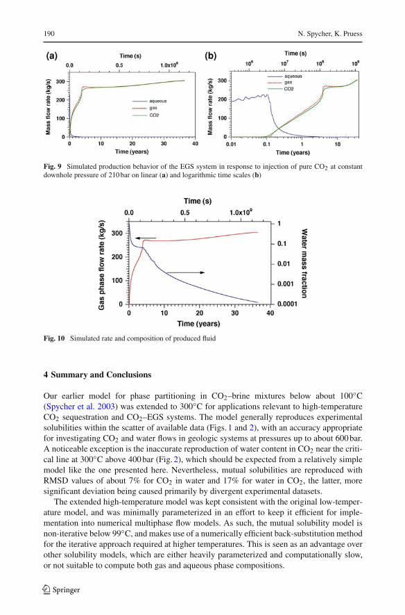
3.2 Results

Simulation results are given in Figs. 9 and 10. Initial fluid production in response to CO2

injection is single-phase water. Breakthrough of CO2 at the production well occurs after 46days, and subsequently a two-phase water–CO2 mixture is produced. Over time, the rate ofgas production increases, while aqueous phase production declines, reflecting relative per-meability effects as gas saturations in the reservoir increase from continuous CO2 injection.After 3.9 years of CO2 injection, aqueous phase production ceases, and subsequently a sin-gle-phase stream of supercritical CO2 is produced. At the time when an aqueous phase ceasesto be produced, the produced CO2 includes approximately 6.4% by weight of dissolved water(Fig. 10). The water content in the produced fluid declines fairly rapidly after aqueous phaseproduction ceases, due to partial reservoir dryout in the fractures, dropping below 1% after7.4 years. The decline of H2O concentrations slows over time, dropping below 0.1% after17.1 years, while at the end of the simulation, after 36.5 years, water content in produced CO2

123

Application to CO2-Enhanced Geothermal Systems 189

Table 4 Parameters for five-spotfractured reservoir

a we include some wall rock inthe definition of the fracturedomain

FormationThickness H = 305 mFracture spacing D = 50 m

Relative permeabilities (Corey 1954)

Liquid krl = S4

Slr = 0.30

Gas krg = (1 − S)2(1 − S2) Sgr = 0.05

where S = (S1 − Slr)/(1 − Slr − Sgr)Capillary pressure (van Genuchten 1980)Pcap = −P0([S1]−1/λ − 1)1−λ

Parameterλ = 0.4438

Strength coefficient for fractures P0,f = 0.0416 barStrength coefficient for matrix P0,m = 6.734 bar

Fracture domainVolume fraction 2%Intrinsic porositya φf = 50%Fracture network permeability kf = 50.0 × 10−15m2

Matrix domainVolume fraction 98 %Intrinsic porosity φm = 1%Matrix permeability km = 1.9 × 10−18m2

Thermal parametersRock grain density ρR = 2, 650 kg/m3

Rock specific heat cR = 1, 000 J/kg/◦CRock thermal conductivity K = 2.1 W/m/◦C

Initial ConditionsReservoir fluid All waterTemperature Tin = 200◦CPressure Pin = 200 bar

Production/InjectionPattern area A = 1 km2

Injector-producer distance L = 707.1 mInjection temperature Tinj = 20◦CInjection pressure (downhole) Pinj = Pin + 10 barProduction pressure (downhole) Ppro = Pin − 10 bar

is 0.012%. Almost half of the initial water inventory in the reservoir still remains in placeafter 36.5 years.

We performed limited sensitivity studies, varying parameters such as strength ofcapillary pressure, and matrix porosity and permeability. We also ran a simulation that in-cluded molecular diffusion of water dissolved in CO2, and CO2 dissolved in water. Theseproblem variations did affect quantitative details of reservoir production behavior, but hadonly limited effects on the water content of produced CO2. While production of a free aque-ous phase from an EGS operated with CO2 will occur for only a limited time (a few years),we conclude that significant dissolved water will persist in the CO2 production stream fordecades.

An attractive possible design for generating electric power from EGS operated with CO2

would directly feed the produced CO2 stream to a turbine, thereby avoiding capital and oper-ating expenses, and heat losses of a heat exchanger. Because our simulations suggest thatsignificant concentrations of dissolved water would persist in the CO2, it will be necessaryto dry the produced fluid upstream of the turbine, akin to removing the “H2O contaminant,”to avoid corrosion from water condensation and carbonic acid formation at the low-P, low-Tside of the turbine.

123

190 N. Spycher, K. Pruess

Fig. 9 Simulated production behavior of the EGS system in response to injection of pure CO2 at constantdownhole pressure of 210 bar on linear (a) and logarithmic time scales (b)

Fig. 10 Simulated rate and composition of produced fluid

4 Summary and Conclusions

Our earlier model for phase partitioning in CO2–brine mixtures below about 100◦C(Spycher et al. 2003) was extended to 300◦C for applications relevant to high-temperatureCO2 sequestration and CO2–EGS systems. The model generally reproduces experimentalsolubilities within the scatter of available data (Figs. 1 and 2), with an accuracy appropriatefor investigating CO2 and water flows in geologic systems at pressures up to about 600 bar.A noticeable exception is the inaccurate reproduction of water content in CO2 near the criti-cal line at 300◦C above 400 bar (Fig. 2), which should be expected from a relatively simplemodel like the one presented here. Nevertheless, mutual solubilities are reproduced withRMSD values of about 7% for CO2 in water and 17% for water in CO2, the latter, moresignificant deviation being caused primarily by divergent experimental datasets.

The extended high-temperature model was kept consistent with the original low-temper-ature model, and was minimally parameterized in an effort to keep it efficient for imple-mentation into numerical multiphase flow models. As such, the mutual solubility model isnon-iterative below 99◦C, and makes use of a numerically efficient back-substitution methodfor the iterative approach required at higher temperatures. This is seen as an advantage overother solubility models, which are either heavily parameterized and computationally slow,or not suitable to compute both gas and aqueous phase compositions.

123

Application to CO2-Enhanced Geothermal Systems 191

As part of this study, a large amount of experimental data on the solubility of CO2 in NaCl(primarily) and CaCl2 solutions were regressed to allow the calculation of mutual solubil-ities of CO2 and water for saline solutions up to about 6 m NaCl. In doing so, correlationsto compute activity coefficients for aqueous CO2 from ∼20 to 300◦C and up to 600 barwere presented. These correlations, together with expressions and parameters developed tocompute equilibrium constants for aqueous CO2, are suitable for implementation into othermodels designed to compute multicomponent geochemical equilibria.

The phase-partitioning correlations developed in this study were implemented into amultiphase flow numerical model to simulate a (hypothetical) CO2-EGS system, in whichdry supercritical CO2 at 20◦C is injected into a 200◦C hot-water reservoir. A 2D horizontalnumerical mesh was developed, comprising one injection and one production well (repre-senting a 1/8 symmetry domain of a 5-spot well pattern), and a fractured reservoir representedby two continua (fractures and matrix). Simulation results show a declining amount of wa-ter and increased CO2 content in produced fluid, with water production ending after about4 years. At this point, about 6% (by weight) water remain in the produced single-phase CO2

stream, decreasing thereafter to <1% after ∼7 years, <0.1% after ∼17 years, and <0.01%after ∼36 years. After this time, almost half of the initial water inventory in the reservoirremains. These results suggest that although water is relatively quickly displaced by the CO2

plume, significant amounts of water may remain dissolved in the produced CO2 phase forlong periods of time. The presence of water in the CO2 would have implications not onlyfor the design of heat extraction systems, but would also dictate the amount of reactivity ofCO2 with the reservoir and engineered systems. For these reasons, future assessment of thepotential for CO2-EGS will need to focus not only on flow/recovery issues, but also on thereactivity of CO2 containing various amounts of water (including dry CO2) with reservoirrocks and other relevant materials.

Acknowledgments We are grateful to Matthew Reagan for an internal review of this article, as well as toDavid Kaszuba and two other anonymous reviewers for their review comments. This study was supportedby Contractor Supporting Research (CSR) funding from Berkeley Lab, provided by the Director, Office ofScience, and by the Zero Emission Research and Technology project (ZERT) under Contract No. DE-AC02-05CH11231 with the U.S. Department of Energy.

Open Access This article is distributed under the terms of the Creative Commons Attribution Noncommer-cial License which permits any noncommercial use, distribution, and reproduction in any medium, providedthe original author(s) and source are credited.

Appendix A—Equation of State and Mixing Rules

The following Redlich–Kwong equation of state is used to compute volume (V ) as a functionof temperature and pressure:

P =(

RTK

V − bmix

)−

(amix

T 0.5K V (V + bmix)

)(A-1)

Equation A-1 is recast as the following cubic expression:

V 3 − V 2(

RTK

P

)− V

(RTKbmix

P− amix

PT 0.5K

+ b2mix

)−

(amix bmix

PT 0.5K

)= 0

(A-2)

123

192 N. Spycher, K. Pruess

Parameters amix and bmix in Eqs. A-1 and A-2 represent measures of intermolecular attractionand repulsion, respectively, and are computed using the mixing rules described below. Otherparameters are as defined earlier. Equation A-2 is solved for the volume of the compressedgas phase (or the stable phase, gas or liquid, below the critical point of CO2) as described inSpycher et al. (2003).

The mixing rules of Panagiotopoulos and Reid (1986) are applied, as reformulated(equivalent) in Orbey and Sandler (1998):

amix =n∑

i=1

n∑j=1

yi y j ai j (A-3)

bmix =n∑

i=1

yi bi (A-4)

with

ai j = √ai i a j j (1 − ki j ) (A-5)

and

ki j = Ki j yi + K ji y j (A-6)

Parameters kii and Kii are always zero (i.e., non-zero values are only for cross-terms) andKi j �= K ji . When Ki j and K ji are set to zero, the mixing rules revert to original van derWaals mixing rules. Parameters ai i , bi , Ki j , and Ki j are expressed as functions of tempera-ture, F(TK), in the form:

F(TK) = a + bTK (A-7)

Note, however, that in the low-temperature model, which is implemented in this study atT < 99◦C, the parameter ai j is not computed using Eq. A-5, and the value of ai j is entereddirectly as a function of temperature (Eq. A-7). In addition, the assumption is made thatyH2O = 0 in the mixing rules and expressions to calculate fugacity coefficients, and there-fore a value of aH2O(ai i for water) is not needed (see Spycher et al. 2003).

The fugacity coefficient, �k , of component k in mixtures with other components i is thencalculated with the following equation after Panagiotopoulos and Reid (1986)2:

ln(�k) = bk

bmix

(PV

RTK− 1

)− ln

(P

(V − bmix)

RTK

)

+

⎛⎜⎜⎜⎝

n∑i=1

yi (aik +aki )−n∑

i=1

n∑j=1

y2i y j (ki j −k ji )

√ai a j +xk

n∑i=1

xi (kki −kik)√

ai ak

amix− bk

bmix

⎞⎟⎟⎟⎠

×(

amix

bmix RT 1.5K

)ln

(V

V + bmix

)(A-8)

2 In the denominator of the fourth term of Eq. A-8, TK is raised to the power 1.5, whereas it is not in theequation given by Panagiotopoulos and Reid (1986). This is because these authors use a form of the Redlich–Kwong equation of state that does not include a T 0.5

K term in the denominator of its second term, as it does inEq. A-1.

123

Application to CO2-Enhanced Geothermal Systems 193

Appendix B—Extension for Saline Solutions

Equations 8 and 9 are replaced by (Spycher and Pruess 2005)

yH2O = A(1 − xCO2 − xsalt) (B-1)

xCO2 = B ′(1 − yH2O) (B-2)

where A and B ′ are defined by Eqs. 10 and 17, respectively. The salt mole fraction, xsalt , isdefined on the basis of a fully dissociated salt, with

xsalt = υmsalt

55.508 + υmsalt + mCO2(aq)

(B-3)

mCO2 = xCO2 55.508

xH2O(B-4)

xH2O = 1 − xCO2 − xsalt (B-5)

where υ is the stoichiometric number of ions contained in the dissolved salt (i.e., 2 forNaCl, 3 for CaCl2, etc.) Alternatively, we can also write

mCO2 = xCO2(υmsalt + 55.508)

(1 − xCO2)(B-6)

Equations B-1 and B-2 are solved by substitution, yielding (Spycher and Pruess 2005)

yH2O = (1 − B′)55.508

(1/A − B′)(υ msalt + 55.508) + υ msaltB′ (B-7)

Therefore, for saline systems, Eqs. B-7 and B-2 replace Eqs. 16 and 9, respectively,developed for the pure-water system.

References

Audigane, P., Gaus, I., Czernichowski-Lauriol, I., Pruess, K., Xu, T.: Two-dimensional reactive transport mod-eling of CO2 injection in a saline aquifer at the sleipner site, North Sea. Am. J. Sci. 307, 974–1008 (2007)

Bachu, S., Bennion, B.: Effects of in-situ conditions on relative permeability characteristics of CO2-brinesystems. Environ. Geol. 54(8), 1707–1752 (2008)

Bando, S., Takemura, F., Nishio, M., Hihara, E., Akai, M.: Solubility of CO2 in aqueous solutions of NaCl at30 to 60◦C and 10 to 20 MPa. J. Chem. Eng. Data 48, 576–579 (2003)

Blencoe, J.G., Naney, M.T., Anovitz, L.: The CO2–H2O system: III. A new experimental method for deter-mining liquid-vapor equilibria at high supercritical temperatures. Am. Mineral. 86, 1100–1111 (2001)

Brown, D.W.: A hot dry rock geothermal energy concept utilizing supercritical CO2 instead of water. Proceed-ings, twenty-fifth workshop on geothermal reservoir engineering, Stanford University, January 2000, pp.233–238

Carlson, H., Colburn, A.P.: Vapor-liquid equilibria of nonideal solutions: utilization of theoretical methods toextend data. Ind. Eng. Chem. 34, 581–589 (1942)

Chiquet, P., Daridon, J.L., Broseta, D., Thibeau, S.: CO2/water interfacial tensions under pressure and tem-perature conditions of CO2 geological storage. Energy Convers. Manage. 48, 736–744 (2007)

Coan, C.R., King, A.D. Jr.: Solubility of water in compressed carbon dioxide, nitrous oxide, and ethane.Evidence for hydration of carbon dioxide and nitrous oxide in the gas phase. J. Am. Chem. Soc. 93, 1857–1862 (1971)

Corey, A.T.: The interrelation between gas and oil relative permeabilities. Producers Monthly, pp. 38–41,November 1954

Cramer, S.D.: The solubility of methane, carbon dioxide, and oxygen in brines from 0 to 300◦C. Report ofinvestigations 8706, U.S. Department of the Interior, Bureau of Mines (1982)

123

194 N. Spycher, K. Pruess

Denbigh, K.: The principles of chemical equilibrium, 4th ed. Cambridge University Press, 494 pp. (1983)Doherty, J.: PEST—model-independent parameter estimation. Watermark Numerical Computing, Corinda

4075, Brisbane, Australia (2008) http://www.sspa.com/pest/Drummond, S.E.: Boiling and mixing of hydrothermal fluids: chemical effects on mineral precipitation. Ph.D.

thesis, Pennsylvania State University (1981)Duan, Z., Sun, R.: An improved model calculating CO2 solubility in pure water and aqueous NaCl solutions

from 257 to 533 K and from 0 to 2000 bar. Chem. Geol. 193, 257–271 (2003)Gilfillan, S.M.V., Ballentine, C.J., Holland, G., Blagburn, D., Sherwood Lollar, B., Stevens, S., Schoell, M.,

Cassidy, M.: The noble gas geochemisry of natural CO2 gas reservoirs from the Coloradeau Plateau andRocky Montain provinces, USA. Geochimica Et Cosmochimica Acta 72, 1174–1198 (2008)

Fenghour, A., Wakeham, W.A., Watson, J.T.R.: Densities of (water + carbon dioxide) in the temperature range415 K to 700 K and pressures up to 35 MPa. J. CHem. Thermodynamics 28, 433–446 (1996)

Fouillac, C., Sanjuan, B., Gentier, S., Czernichowski-Lauriol, I.: Could sequestration of CO2 be combined withthe development of enhanced geothermal systems? In: Paper presented at the Third Annual Conferenceon Carbon Capture and Sequestration, Alexandria, Virginia, May 3–6, 2004

Gehrig, M., Lentz, H., Frank, E.U.: The system water-carbon dioxide-sodium chloride to 773 K and300 MPa. Ber. Bunsenges. Phys. Chem. 90, 525–533 (1986)

Gérard, A., Genter, A., Kohl, T., Lutz, P., Rose, P., Rummel, F.: The deep EGS (Enhanced Geothermal System)project at Soultz-sous-Forets (Alsace, France). Geothermics 35(5-6), 473–483 (2006)

Gillepsie, P.C., Wilson, G.M.: Vapor-liquid and liquid-liquid equilibria: water-methane, water-carbon dioxide,water-hydrogen sulfide, water-npentane, water-methane-npentane. Research report RR-48, Gas Proces-sors Association, Tulsa Okla, April (1982)

Giorgis, T., Carpita, T., Batistelli, A.: 2D modeling of salt precipitation during injection of dry CO2 in adepleted gas reservoir. Energy Conserv. Manage. 48, 1816–1826 (2007)

Goyal, K.: Injection recovery factors in various areas of the Southeast Geysers, California. Geother-mics 24, 167–186 (1995)

Hurter, S., Labregere, D., Berge, J.: Simulations of dry-out and halite precipitation due to CO2 injection. Geo-chimica Et Cosmochimica Acta 71, A426–A426 (2007)

Hu, J., Duan, Z., Zhu, C., Chou, I.-M.: PVTx properties of the CO2–H2O and CO2–H2O-NaCl systems below647 K: assessment of experimental data and thermodynamic models. Chem. Geol. 238, 249–267 (2007)

IPCC: Carbon dioxide capture and storage In: Metz, B., Davidson, O., de Coninck, H., Loos, M., Meyer, L.(eds.) Prepared by Working Group III of the Intergovernmental Panel on Climate Change, CambridgeUniversity Press, 431 pp. (2005)

IPCC: Climate change 2007: synthesis report. Contributions of working groups I, II, and III to thefourth assessment report of the intergovernmental panel on climate change. In: Core Writing Team,Pachauri, R.K., Reisinger, A. (eds.) Intergovernmental Panel on Climate Change, c/o World Meteoro-logical Organization, Geneva, Switzerland, 104 pp. (2008)

Kaszuba, J.P., Janecky, D.R., Snow, M.G.: Carbon dioxide sequestration processes in a model brine aqui-fer at 200◦C and 200 bars: implications for geologic sequestration of carbon. Applied Geochemistry18:1065–1080 (2003)

Kiepe, J., Horstmann, S., Fisher, K., Gmehling, J.: Experimental determination and prediction of gas solubil-ity data for CO2 + H2O mixtures containing NaCl or KCl at temperatures between 313 and 393 K andpressures up to 10 MPa. Ind. Eng. Chem. Res. 41, 4393–4398 (2003)

Koschel, D., Coxam, J.-Y., Rodier, L., Majer, V.: Enthalpy and solubility of CO2 in water and NaCl(aq) atconditions of interest for geological sequestration. Fluid Phase Equilibria 247, 107–120 (2006)

Lin, H., Fujii, T., Takisawa, R., Takahashi, T., Hashida, T.: Experimental evaluation of interactions in supercriti-cal CO2/water/rock mineral system under geologic CO2 sequestration conditions. J. Mater. Sci. 43, 2307–2315 (2008)

Malinin, S.D., Kurovskaya, N.A.: Investigations of CO2 solubility in a solution of chlorides at elevated tem-peratures and pressures of CO2. Geokhimiya 4, 547–551 (1975)

Malinin, S.D., Savelyeva, N.I.: The solubility of CO2 in NaCl and CaCl2 solutions at 25, 50, and 75◦C underelevated CO2 pressures. Geokhimiya 6, 643–653 (1972)

Malinin, S.D.: The system water-carbon dioxide at high temperatures and pressures. Geokhimiya 3, 235–245 (1959)

Markham, A.E., Kobe, K.A.: The solubility of carbon dioxide and nitrous oxide in aqueous salt solutions.J. Am. Chem. Soc. 63, 449–454 (1941)

Müller, G., Bender, E., Maurer, G.: Das Dampf-Flüssigkeitsgleichgewicht des ternären Systems Ammoniak-Kohlendioxid-Wasser bei hohen Wassergehalten im Bereich zwischen 373 und 473 Kelvin. Berichte derBunsen-Gesellshaft für Physikalische Chemie 92, 148–160 (1988)

MIT (ed.): The Future of Geothermal Energy. (Massachusetts Institute of Technology, Cambridge, MA 2006)

123

Application to CO2-Enhanced Geothermal Systems 195

Moore, J. Adams, Allis, R., Lutz, S., Rauzi, S.: Mineralogical and geochemical consequences for the long-termpresence of CO2 in natural reservoirs: an example from the Spingville-St. Johns Field, Arizona, and NewMexico, U.S.A.. Chem. Geol. 217, 365–385 (2005)

Nickalls, R.W.D.: A new approach to solving the cubic: Cardan’s solution revealed. Math. Gaz. 77, 354–359 (1993)

Nighswander, J.A., Kalogerakis, N., Mehotra, A.K.: Solubilities of carbon dioxide in water and 1 wt% NaClsolution at pressures up to 10 MPa and temperatures from 80 to 200◦C. C. J. Chem. Eng. Data 34, 355–360 (1989)

Orbey, H., Sandler, S.I.: Modeling Vapor-Liquid Equilibria: Cubic Equations of State and their Mixing Rules.Cambridge University Press (1998)

Palandri, J., Rosenbauer, R.J., Kharaka, Y.K.: Ferric iron in sediments as a novel CO2 mineral trap: CO2–SO2reaction with hematite. Appl. Geochem. 20, 2038–2048 (2005)

Panagiotopoulos, A.Z., Reid, R.C.: New mixing rules for cubic equations of state for highly polar asymmetricmixtures. ACS Symposium Series 300: American Chemical Society, Washington, D.C., pp. 571–582(1986)

Pruess, K.: Numerical simulation of multiphase tracer transport in fractured geothermal reservoirs. Geother-mics 31, 475–499 (2002)

Pruess, K.: The TOUGH codes—a family of simulation tools for multiphase flow and transport processes inpermeable media. Vadose Zone J. 3, 738–746 (2004)

Pruess, K.: Enhanced geothermal systems (EGS) using CO2 as working fluid—a novel approach for generatingrenewable energy with simultaneous sequestration of carbon. Geothermics 35(4), 351–367 (2006)

Pruess, K.: On production behavior of enhanced geothermal systems with CO2 as working fluid. EnergyConvers. Manage. 49, 1446–1454 (2008)

Pruess, K., Narasimhan, T.N.: A practical method for modeling fluid and heat flow in fractured porousmedia. Soc. Pet. Eng. J. 25(1), 14–26 (1985)

Pruess, K., Spycher, N.: ECO2N—a fluid property module for the TOUGH2 code for studies of CO2 storagein saline aquifers. Energy Convers. Manage. 48(6), 1761–1767 (2007)

Pruess, K., Müller, N.: Formation dry-out from CO2 injection into saline aquifers: 1. Effects of solids precip-itation and their mitigation. Water Resour. Res. 45, W03402, doi:10.1029/2008WR007101 (2009)

Prutton, C.F., Savage, R.L.: The solubility of carbon dioxide in calcium chloride-water solutions at 75, 100,120◦C and high pressures. J. Am. Chem. Soc. 67, 1550–1554 (1945)

Regnault, O., Lagneau, V., Catalette, H., Schneider, H.: Etude expérimentale de la réactivité du CO2 supercri-tique vis-à-vis de phases minérales pures Implications pour la séquestration géologique de CO2. ComptesRendus Geosci. 337, 1331–1339 (2005)

Rimmelé, G., Barlet-Gouédard, V., Porcherie, O., Goffé, B., Brunet, F.: Heterogeneous porosity distributionin Portland cement exposed to CO2-rich fluids. Cem. Concr. Res. 38, 1038–1048 (2008)

Rosenbauer, R.J., Koksalan, T., Palandri, J.L.: Experimental investigation of CO2-brine-rock interactions atelevated temperature and pressure: Implications for CO2 sequestration in deep-saline aquifers. FuelProcess. Technol. 86, 1581–1597 (2005)

Rumpf, B., Nicolaisen, H., Ocal, C., Maurer, G.: Solubility of carbon dioxide in aqueous solutions of sodiumchloride: experimental results and correlation. J. Solut. Chem. 23, 431–448 (1994)

Sako, T., Sugeta, T., Nakazawa, N., Obuko, T., Sato, M., Taguchi, T., Hiaki, T.: Phase equilibrium study ofextraction and concentration of furfural produced in reactor using supercritical carbon dioxide. J. Chem.Eng. Jpn. 24, 449–454 (1991)

Shagiakhmetov, R.A., Tarzimanov, A.A.: Deposited document SPSTL 200 khp-D 81-1982 (1981). Summa-rized in: Sharlin, P.: Carbon Dioxide in Water and Aqueous Electrolyte Solutions. Solubility Data Series,vol. 62, 383 pp. International Union of Pure and Applied Chemistry, Oxford University Press (1996)

Span, R., Wagner, W.: A new equation of state for carbon dioxide covering the fluid region from the triple-pointtemperature to 1100 K at pressures up to 800 MPa. J. Phys. Chem. Ref. Data 25(6), 1509–1596 (1996)

Spycher, N., Pruess, K.: Mixtures in the geological sequestration of CO2. II. Partitioning in chloride brines at12–100◦C and up to 600 bar. Geochimica Et Cosmochimica Acta 69, 3309–3320 (2005)

Spycher, N., Pruess, K., Ennis-King, J.: CO2–H2O Mixtures in the geological sequestration of CO2. I. Assess-ment and calculation of mutual solubilities from 12 to 100◦C and up to 600 bar. Geochimica Et Cosmo-chimica Acta 67, 3015–3031 (2003)

Stark, M.A., Box, W.T. Jr., Beall, J.J., Goyal, K.P., Pingol, A.S.: The Santa Rosa–Geysers recharge project,Geysers geothermal field, California, USA. Proceedings, file 2420.pdf, World Geothermal Congress,Antalya, Turkey, April 2005

Suto, Y., Liu, L., Yamasaki, N., Hashida, T.: Initial behavior of granite in response to injection of CO2-saturatedfluid. Appl. Geochem. 22, 202–218 (2007)

123

196 N. Spycher, K. Pruess

Takenouchi, S., Kennedy, G.C.: The binary system H2O–CO2 at high temperatures and pressures. Am.J. Sci. 262, 1055–1074 (1964)

Takenouchi, S., Kennedy, G.C.: The solubility of carbon dioxide in NaCl solutions at high temperatures andpressures. Am. J. Sci. 263, 445–454 (1965)

Tödheide, K., Frank, E.U.: Das Zweiphasengebiet und die kritische Kurve im System Kohlendioxid-Wasserbis zu Drucken von 3500 bar. Z. Phys. Chemie, Neue Folge 37, 387–401 (1963)

van Genuchten, M.Th.: A closed-form equation for predicting the hydraulic conductivity of unsaturatedsoils. Soil Sci. Soc. Am. J. 44, 892–898 (1980)

Vorholz, J., Harismiadis, V.I., Rumpf, B., Panagiotopoulos, A.Z., Maurer, G.: Vapor + liquid equilibrium ofwater, carbon dioxide, and the binary system, water + carbon dioxide, from molecular simulation. FluidPhase Equilibria 170, 203–234 (2000)

Wagner, W., Pruss, A.: The IAPW formulation 1995 for the thermodynamic properties of ordinary watersubstance for general scientific use. J. Phys. Ref. Data 31, 387–535 (2002)

Webb, S.W.: A simple extension of two-phase characteristic curves to include the dry region. Water Resour.Res. 36(6), 1425–1430 (2000)

Wiebe, R., Gaddy, V.L.: The solubility in water of carbon dioxide at 50, 75, and 100◦, at pressures to 700atmospheres. J. Am. Chem. Soc. 61, 315–318 (1939)

123