A numerical study of optimized sparse preconditioners

BIT34 (1994), 177-204.

A NUMERICAL STUDY OF OPTIMIZED SPARSE PRECONDITIONERS

A. M. BRUASET* and A. TVEITOt

SINTEF, P.O. Box 124, Blindern, N-0314 Oslo, Norway email: [email protected] no, Aslak. [email protected] no.

Abstract.

Preconditioning strategies based on incomplete factorizations and polynomial approximations are studied through extensive numerical experiments. We are concerned with the question of the optimal rate of convergence that can be achieved for these classes of preconditioners.

Our conclusion is that the well-known Modified Incomplete Cholesky factorization (MIC), cf. e.g., Gustafsson [20], and the polynomial preconditioning based on the Chebyshev polynomials, cf. Johnson, Micchelli and Paul [22], have optimal order of convergence as applied to matrix systems derived by discretization of the Poisson equation. Thus for the discrete two-dimensional Poisson equation with n unknowns, O(n '/') and O(n~9 seem to be the optimal rates of convergence for the Conjugate Gradient (CG) method using incomplete factofizations and polynomial preconditioners, respectively. The results obtained for polynomial preconditioners are in agreement with the basic theory of CG, which implies that such preconditioners can not lead to improvement of the asymptotic convergence rate.

By optimizing the preconditioners with respect to certain criteria, we observe a reduction of the number of CG iterations, but the rates of convergence remain unchanged.

AMS subject classification: 65F10, 15A06, 65F90, 65K10

Key words: Conjugate gradient method, preconditioning, incomplete factorization, polynomial preconditioner, matrix-free method, Fourier analysis.

1. Introduction.

In the present paper we are concerned with efficient strategies for iterative solution of the linear system of equations

(1 .1) A x = b,

where A c Rn, n is symmetric and positive definite (SPD). In particular we will restrict our attention to difference approximations of the generic model problem

(1.2) --Au(x, y) = f (x , y)

* Supported by The Norwegian Research Council for Science and the Humanities (NAVF) under grants no. 413.90/002 and 412.93/005.

t Supported by The Royal Norwegian Council for Scientific and Industrial Research (NTNF) through program no. STP.28402: Toolldts in industrial mathematics.

Received April 1993. Revised December 1993.

178 A.M. BRUASET AND A. TVEITO

defined on the unit square fl = [0, 1] 2 with suitable boundary conditions. Problems like (1.1) are commonly solved by the preconditioned conjugate gradient (PCG) method, cf. Concus et al. [13], thus directing our concern to the choice of a proper preconditioner.

When preconditioning the system (1.1), we search for a nonsingular matrix M ~ R"." such that the transformed system

M - l A x = M - l b

can be solved in fewer PCG iterations than needed for the original problem. To do this we can choose either an i m p l i c i t or exp l i c i t method. In this context the term "implicit" refers to a preconditioning matrix M which in some sense approximates the original coefficient matrix A, such that a system of the form M t = r has to be solved in each PCG iteration. The solution of these inner systems will be a very time-consuming part of the overall process, thus suggesting that M could be represented by some LU factorization such that M t =

r is reduced to two triangular systems. This concept is used by preconditioning techniques based on the so called incomplete Cholesky factorizations IC, MIC and RIC, of. papers by Meijerink and van der Vorst [25], Gustafsson [20], Axelsson and Lindskog [8]. The idea of IC is to compute the Cholesky decom- position L L r of A except that L is allowed to have non-zero entries only in some predefined matrix positions. Usually one chooses the sparsity pattern of L equal to that of the lower triangular part of A. This procedure is denoted by IC(0), while IC(k), k > 0, indicates that L is allowed to have k extra non-zero diagonals. Regarding MIC factorization, L is computed as the incomplete Cho- lesky factor o fA + ~h2I where ~ > 0 is a problem-dependent parameter, ~ of. Chan and Elman [ 12]. The RIC strategy generalizes the IC and MIC methods by introducing a relaxation parameter w, such that certain choices ofo~ reproduce the other two factorizations; see Chan [11]. As for the IC factorization it is possible to extend the support of the MIC or RIC factors to get MIC(k) and RIC(k).

An alternative to the factorized precondifioners that has received much attention in recent years, is to establish a sparse matrix M - ~ which approximates A -1. For such preconditioners, which are referred to as being "explicit", the inner system is solved by direct computation of the product t -- M-~r. This property makes such methods very attractive for implementation on vector and/or parallel computers, whereas the implicit procedures may reduce the potential of such architectures. The explicit preconditioner M-I can for instance be a diagonal scaling, of. Pini and Gambolatti [27], a truncated Neumann series for A-I, cf. Dubois et al. [ 17], or a matrix-valued polynomial, of. Johnson et al. [22].

Supposing we have the splitting A = I - G where A is scaled to have unit

In the case of our model problem the optimal choice is ~ ~ 2~r 2 for Dirichlet boundary conditions and ~ ~ 8~r 2 for the periodic case. Throughout this paper we apply the proper optimal value whenever MIC is used.

A NUMERICAL STUDY OF OPTIMIZED SPARSE PRECONDITIONERS 17 9

diagonal, we want to pursue the latter idea of using M~ ~= Z~o ajGJ as a polynomial approximation to A- ~. There are many possible choices of the coefficients a0, al . . . . , am. In [22], Johnson et al. search for the ruth degree polynomial preconditioner

(1.3) ~ 1 ~ %GJ = ~ 6,A' = tim(A) j=O 1=0

that minimizes the spectral condition number K(Mv,1A) for all relevant coefficients. They use the formulation MT~ 1A = Pm(A)A -- IP(A) to define the associated scalar min-max approximation problem

min max I1 - 9a(a)[, P~*rm+ 1 a~S 9(0)=0

where ~rk denotes the set of real polynomials of degree -<k and S = [S~ , Sin=] is a set including the eigenvalue spectrum of A. This approximation problem is known to have the solution

where Tk is the kth degree Chebyshev polynomial of the first kind. Ideally, Smm and Smax would be equal to the extreme eigenvalues of A. Since the optimal preconditioning polynomial is now given as PmO) = 7'(a)/a, the coefficients fij (or %) in (1.3) are computable. For other types of polynomial preconditioners see works by Ashby and others [2, 3, 5, 6] and O'Leary [26]. These papers also discuss the use of adaptive procedures where the best possible polynomial preconditioner is determined dynamically by the algorithm itself.

Many of the preconditioning methods introduced above have proven to be very useful for a large number of applications. However, we may ask whether these established methods fully exploit the potential of the basic strategies of incomplete factorization and polynomial approximation. Such questions have also been asked by other authors, e.g., Greenbaum and Rodrigue [19], and the efforts to find answers range from theoretical considerations to numerical experiments. As far as the heuristic approach of numerical optimization of preconditioners is concerned, the results have suffered from being based on a very limited number of observations. This is mainly caused by the very high computational cost of such experiments. Even when applying an efficient optimization code, the computation will frequently need updated estimates for the eigenvalues of the preconditioned operator. If such information is not available as analytic expressions, the eigenvalues have to be approximated numerically by algorithms that usually are very demanding in terms of computing time and storage. Such limitations put severe restrictions on the problem size n and encourage optimization criteria that use only a few eigenvalues, e.g., minimization of the condition number. Other relevant criteria that require full spectral information are in this case practically disqualified.

180 A. M. BRUASET AND A. TVEITO

The present paper combines the experimental approach with a model problem that through Fourier analysis provides us with explicit expressions for the eigenvalue spectrum of M-1A. We will only be concerned with the existence of optimized preconditioners of Cholesky factored form or polynomial form, and to what extent some established preconditioners are efficient representa- tives of their respective families. From this viewpoint we do not care whether the construction of a certain preconditioner is time-consuming or not. How to compute such optimized preconditioning matrices by efficient algorithms, or if such algorithms exist at all, are problems beyond the scope of this work.

For discrete elliptic problems with constant coefficients and periodic boundary conditions, numerical solution methods can be studied by techniques based on Fourier analysis. A paper by Chan and Elman [12] shows that this approach can give valuable insight into existing methods. Fourier analysis of iterative solvers for discrete elliptic problems is also discussed by Donato and Chan [16], and in [11] this technique provides the optimal RIC parameter o~ that minimizes the condition number. A similar strategy has been applied to solution procedures for linear systems arising when interpolating a data set with box splines, see Arge et al. [ 1 ]. As reported in these papers, the eigenvalue distribution of the model problem (1.2) with Dirichlet boundary conditions is closely related to the spectrum of the corresponding periodic problem. In fact, the convergence behaviour of the Dirichlet problem with mesh size h d c a n be estimated from the results for the periodic problem with mesh size hp, when hd = 2hp.

In Section 2 we use the Fourier approach to develop closed expressions for the eigenvalues of the preconditioners we want to examine. These expressions will be functions of a small number of free parameters that completely describe the preconditioners in question. From this basis we formulate in Section 3 several criteria for the selection of a preconditioning matrix. These criteria rely on detailed knowledge of the spectrum of M-IA, and thus constitute object functions that depend on the preconditioner's parameters. These functions, as well as the residual norm obtained after a fixed number of PCG iterations, are in Section 4 subject to a large number of numerical experiments using a standard algorithm for minimization. The resulting preconditioners are evaluated by their respective convergence rates in terms of the number of PCG iterations needed to reach a prescribed numerical accuracy. As a complement to the heuristics found in I11, 12, 16], we also compare the object functions defined in Section 3 with respect to boundary conditions. Observing that the construction of optimized preconditioners seems to be relatively insensitive to whether we have Dirichlet or periodic boundary conditions, we expect that the Fourier- based results provide valuable information even for the Dirichlet case.

2. Fourier analysis of gridpoint operators.

2.1. Gridpoint operators.

In this section, we consider the model problem (1.2) subject to the periodic boundary conditions

Figure 2.1.

A NUMERICAL STUDY OF OPTIMIZED SPARSE PRECONDITIONERS 181

(i) (II)

k ~ 6 ~7 LOS ~ 7 0-~6

j J

(I) The computational molecule for the periodic Laplacian A. (II) The gridpoint operator B(o~).

(2.1) u ( x , O) = u ( x , 1), u(O, y ) = u (1 , y ) .

When discretizing this problem using centered differences on a uniform grid with mesh size h = 1/ (q + 1), we derive a linear system of equations of order n = (q + 1) 2. Denoting the numerical solution in each gridpoint by Uj, k, the equation corresponding to the node indices (j, k) can be written

1 h 2 (2.2) u,.k - -~ (u ,k_ , + u , _ , , + Ui+,.k + Uj.k+,) = ~ f j . k ,

where fZk = f ( j h , k h ) . The coefficient coefficient matrix A of this system will essentially be a scaled version of the well known pentadiagonal discrete La- placian, except for some entries due to the periodic behaviour of the current problem. Figure 2.1 (I) shows a computational molecule compactly describing the discrete operator A. Throughout this paper we will refer to matrices defined by local recurrences like (2.2) (or their corresponding molecules) by the terms g r i d p o i n t o p e r a t o r or s t enc i l .

When restricting ourselves to a constant coefficient problem with periodic boundary conditions, we may adopt the Fourier based techniques of [1, 1 1, 12, 16] to find analytic estimates for the eigenvalues of the corresponding Dirichlet problem. Consider the periodic gridpoint operator B(o~) with constant weights o~ = (w, . . . . . o~8) depicted in Figure 2. l(II). As will be explained later, this stencil allows us to study the incomplete factorizations IC(I), RIC(I) and MIC(I) for fill-in levels l = 0, 1. Let v ~s,o e R" have entries

v(j{~ t) = eii°~e ik*,, j , k = 0, 1 . . . . . q,

where i is the imaginary unit and

2~rs 27rt O, = ~ = 21rsh, 4~t = ~ = 2~rth

q + l q + l

for s, t = 0, 1 . . . . , q. Inserting v (s,0 into the recurrence for the gridpoint operator B(o~) we find that for each pair of indices (s, t), v (~,o is an eigenvector of B(o~),

182 A . M . BRUASET A N D A. TVEITO

k ~74

~1 7}2 7~3

J

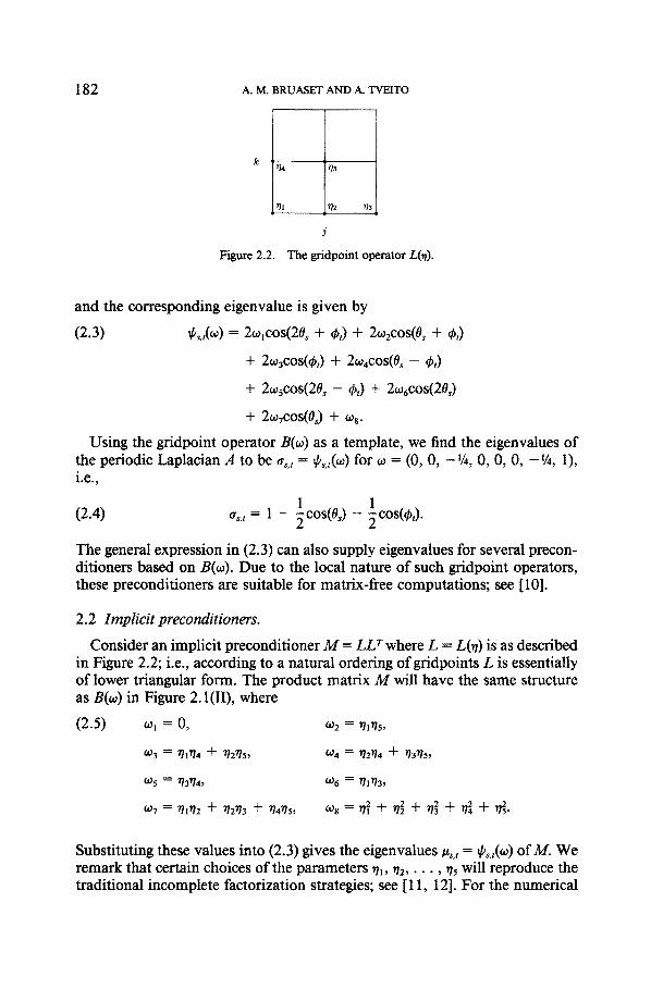
Figure 2.2. The gridpoint operator L(~).

and the corresponding eigenvalue is given by

(2.3) ff~.t(0)) = 20)~cos(20s + ~t) + 20)2cos(0s + ~t)

+ 20)3COS(qSt) + 20)4COS(0 s - - ~bt)

+ 20)~cos(20~ - St) + 20)6cos(20,)

+ 20)7COS(0s) + 0)8"

Using the gridpoint operator B(0)) as a template, we find the eigenvalues of the periodic Laplacian A to be a,., = ff,.t(0)) for 0) = (0, 0, - V4, 0, 0, 0, - l/a, 1), i.e.,

1 1 (2.4) a,,t = 1 - ~cos(O,) - ~cos($t).

The general expression in (2.3) can also supply eigenvalues for several preconditioners based on B(0)). Due to the local nature o f such gridpoint operators, these preconditioners are suitable for matrix-free computat ions; see [10].

2.2 Implicit preconditioners.

Consider an implicit precondit ioner M = LL r where L = L(7) is as described in Figure 2.2; i.e., according to a natural ordering o f gridpoints L is essentially o f lower triangular form. The product matrix M will have the same structure as B(0)) in Figure 2.1 (II), where

(2.5) 0)~ = 0,

0)3 = ~/d/4 + ~/27/5,

005 ~ 73~4,

0)7 = 1~11~2 "~ 71273 "~- 1~475,

0)2 = 7175,

0)4 = ~/d/4 + 7/3~5,

0)6 = 7173,

0)8 = ~ + ~ + ~ + ~ + ~ .

Substituting these values into (2.3) gives the eigenvalues #~,t = ~.t(oJ) of M. We remark that certain choices o f the parameters 71, 72 . . . . ,75 will reproduce the traditional incomplete factorization strategies; see [ 11, 12]. For the numerical

A NUMERICAL STUDY OF OPTIMIZED SPARSE PRECONDITIONERS 1 8 3

experiments in Section 4 we will use two different stencils for L(n), • -- (0, Ii, 0,/2, 1) and n = (0, It, 12,/3, 1), thus utilizing the familiar sparsity patterns of IC(0), MIC(0), RIC(0), and IC(1), MIC(1), RIC(I), respectively. Fixing the diagonal entry 75 = 1 will reduce the number of free parameters in the optimization process, as well as making it possible to compare the computed stencil values of different preconditioners, see the appendix.

REMARK 2.1. Throughout this paper, our study of implicit strategies is restricted to preconditioners of the form described above. For that reason, the current class ofpreconditioners does not include the implicit method of ADDKR; cf. Chan and Elman [1 2]. This procedure, which for the periodic model problem gives a condition number of order O(h-V3), combines a standard MIC factorization with an incomplete factorization for a permuted version of A.

2.3. Explicit preconditioners.

In the class of explicit preconditioners we consider matrix-valued polynomial approximations to A -1. Let

(2.6) MT, ~ = ~ ajG~ j=0

where G is defined by the splitting A = I - G and A is scaled to have all diagonal entries equal to one. In the case of our test problem, this means that G = B(00) for ~0 = (0, 0, 1/4, 0, 0, 0, 1/4, 0). The eigenvalues of the preconditioner Mg ~ are then given by

(2.7) ~Ztl = ~ aj[c°s(0s) + c°s(~')-] j i=o 2 '

where the bracketed expression represents the corresponding eigenvalues of G which are easily derived from (2.3).

When using the traditional PCG implementation, the preconditioner is re- quired to be symmetric positive definite; see e.g., Ashby et al. [7]. For this reason, we will force suitable bounds on the coefficients % in (2.6), such that Mg 1 is positive definite. In order to obtain an efficient polynomial preconditioner that is numerically stable, the power form in (2.6) is not suitable. Instead, under certain assumptions on orthogonality, we may implement such preconditioners in terms of an m-step inner iteration; see Ashby et al. [5]. The preconditioning polynomials constructed in Section 4 do not fit into this framework, thus suggesting the use of the nested form equivalent to (2.6); cf. Conte and de Boor [14, Ch. 2, 6].

3. Criteria for the selection of a preconditioner.

Given the system Ax = b, where A is the discrete Laplacian subject to Dirichlet boundary conditions, we are concerned with the selection of a preconditioner

1 8 4 A.M. BRUASET AND A. TVEITO

M suitable for use with the PCG procedure. Since the eigenvalues Xs., of the preconditioned operator M-~A will be significant to the convergence rate, we want to utilize the results derived in the previous section for the periodic model problem. From the strong correlation between the eigenvalue spectra for the Dirichlet case and the periodic case, it is natural to approximate the Dirichlet eigenvalues with the periodic eigenvalues

(3.1) X,., = o.,,,1#,,,,

which are given for s, t = O, 1 , . . . , q by the results (2.3)-(2.7). We note that problem (1.2) is not well posed for periodic boundary conditions, since u = w + c is a solution for every c ~ R if w is a solution itself. This fact is reflected in the zero eigenvalue (2.4) obtained for s = t -- 0, indicating the singularity of the periodic operator. In order to use the periodic eigenvalues as approximations to the Dirichlet eigenvalues, we restrict the indices to 1 <-- s, t - q.

REMARK 3.1. Although both A and M are SPD in case of Dirichlet boundary conditions, the preconditioned operator M - ~A is in general not SPD. However, since M-~A is similar to the SPD matrix M - V ' A M -V', the Dirichlet eigenvalues are positive and real. By construction, this property is also present for the periodic eigenvalues defined in (3.1).

3.1. M i n i m i z i n g the condition number.

From the analysis o f the PCG method we know that the error after k iterations, e k = x - x k, satisfies the inequality -{X/KA(M-1A)--I)k+ (3.2) llekL _< 2tX/KA(M_~A ) lie°[[A,

where IlellA = (erAe) v: and

max=+o(M-~Az, z) KA(M-1A) =

min~+o(M-1Az, z)

denotes the A-condition number of M-~A; of. Ashby et al. [4]. For simplicity, the term "condition number" will hereafter refer to KA.

Based on (3.2), an intuitive criterion for the selection of a proper preconditioner is to choose M such that ~A is close to one, which makes the upper bound small. This is used by Greenbaum and Rodrigue [19] to motivate the search for an efficient preconditioner through numerical minimization of KA. However, the error bound (3.2) is not sharp, such that a small condition number is suffuzient but not necessary to obtain fast convergence. For a sharp error bound one must utilize the complete eigenvalue distribution and not only the extreme values of the spectrum; el. [9, 18, 21, 29, 30]. Greenbaum [18] gives the precise error estimate in terms of the complete spectrum of M-~A, but it seems difficult to use this information to derive the best possible preconditioner M.


3.2. Minimizing a clustering function. As an alternative to minimizing KA(M-~A), one can define other measures of

preconditioning quality that use all available information about the eigenvalues. It is well-known that the conjugate gradient iteration may possess a superlinear convergence rate when applied to certain linear operators on a Hilbert space. This effect may be observed when the operator has eigenvalues clustered around X = 1; see Winther [31 ]. These results are complemented by numerical observations, cf. Axelsson and Lindskog [8], and motivate the selection criteria presented below.

REMARK 3.2. For a finite dimensional problem like (1.1) the notion of "superlinear convergence" is not fully appropriate. Nevertheless, this term is used also for such problems to describe that the rate of convergence improves during the conjugate gradient process; cf. van der Sluis and van der Vorst [30] and references therein.

Restricting M to be of the form B(o~) indicated in Figure 2.1(II), or M -~ to be a ruth degree polynomial approximation to A -~, we define clustering functions that are closed expressions depending on the free parameters (%}~=~ or {aj}g~, respectively. Through minimization of these functions we are able to force the eigenvalues u,.t = m,,(P) sufficiently close to as.,, such that the corresponding parameter vector p will describe an applicable preconditioner for our problem.

An intuitive formulation of such a clustering function is

(3.3) F~.ex,,(p)= ~ (l ~r~'t -~ 2 ,.,-, u,.,(p)]

where the ratio X,,, = a,,t/u,,t is forced close to unity. Minimizing this function, with respect to the parameters describing the preconditioner in question, will be a useful criterion for the selection of explicit preconditioners. In the case of implicit preconditioners, numerical experiments suggest that the clustering function should be expressed in terms of the eigenvalues of the inverse operator, i.e., X~ ~ = t~,.,(p)/as, t. Thus for such preconditioners we will try to minimize the function

(3.4) F~'im~'(P)= s,t=~ ~'¢ (1 U~"(---P)/2.~,,, /

From (2.4) we see that the small eigenvalues of A will approach zero as the grid size q increases, which may deteriorate the preconditioning performance. In order to control this behaviour, we may use another clustering function that puts most weight on the contributions where g,,, is small,

,.,o, , , . , ( p ) ]

This criterion is suitable for explicit preconditioners, while the corresponding

186

function

(3.6)

A. M. BRUASET A N D A. TVEITO

g2,impl(p) ~ ~ (1 ~£s't('--~P)'121 S,t~l ¢TS, t / ¢Ts,t

is applicable in the setting of implicit preconditioning strategies.

R r ~ 3.3. Another possibility is to minimize the least squares error, i.e., using the clustering function

q

F3(P) = ~.~ (t~s,t(P) - Os,t) 2o s,t= l

Experiments show that this procedure is not very useful for implicit preconditioners and that the results obtained for the explicit case are comparable to those obtained for F2,e~p,. Thus we will not elaborate on this particular criterion. Similar comments apply to preconditioners derived by minimizing the max- imum deviation from unity, i.e., max~,, I l - x,,, I or maxs,, [ 1 - ),~ I.

We also note that clustering functions designed for the implicit case should not be used to derive explicit precondifioners and vice versa. Through experiments we find such preconditioning stencils quite inefficient. Obviously, the functions F~,i,,pt and F2,impt a r e identical to their counterparts F~,expl and F2,exp, with each term weighted by XT.t 2.

3.3 M i n i m i z i n g t h e t r a c e - d e t e r m i n a n t rat io.

Another approach to measuring the quality of a preconditioner was recently introduced by Kaporin [23]. He defines the function s

n -1 Z]=I ~j n -ltr M - 1 A (3.7) fl(p) = - > 1.

(II;=~ hi) '/. (det M - ~ A ) '/"

Through an elegant analysis he proves that the kth PCG iterate x k satisfies the error bound

ilrkll~_, <_ (fl.:k _ 1)k:ZllrOll~_,,

where r k = b - A x k and Ilrll~-, = ( r r M - ~ r ) '/'. From this error estimate it is natural to search for a preconditioner that gives a small value of/~, i.e., we want to minimize # = /~(p) with respect to the parameters p describing the preconditioner. For another application of this measure to describe the deviation of an SPD matrix from the identity, we refer to Dennis and Wolkowicz [151.

4. Nulnerieal experiments.

Based on the framework described in the two previous sections we have performed a large number of numerical experiments with a two-part goal in mind:

The sequence {~j}7-t is a simple reordering of the eigenvalues ~,,., = a.,/t~.,(p), s. t = 1, 2 . . . . . q.


• Using a standard optimization code we want to find preconditioners for- mulated by local gridpoint operators that are "optimal" with respect to the selection criteria stated above. In all cases we look for two types of preconditioners: the incomplete factorizations M = L(n)L(~) r given by Figure 2.2 and (2.5) with n = (0, ll, 0,/2, 1) or n = (0, l~,/2, ls, 1), and the matrices MT, ~, m = 1, 2 , . . . , 5, based on polynomial approximations of A - 1

• Once the optimized preconditioners are computed, the quality of these are tested in terms of the condition numbers KA(M-~A) and the number of PCG iterations needed to fulfill the convergence condition II rk l] 2 -- 10 - 6 II r° II 2- In all cases we compare our results with appropriate established preconditioning strategies.

For easy reference we denote the four criteria for selection ofa preconditioner by the letters (a)-(d), such that the corresponding optimization problem is to minimize the

(a) condition number Ka(M-~A), (b) clustering function F~xx~x given by (3.3) or the clustering function F~,l,~l

given by (3.4), (c) clustering function Fz,expt given by (3.5) or the clustering function F2,,,,p~

given by (3.6), (d) trace-determinant ratio/3 given by (3.7).

Once again we emphasize that the procedure described above for the construction of preconditioners is by no means meant to be of immediate practical use, but a tool for investigating the potential of some widely used classes of preconditioners.

The experiments reported in this section were performed on a DECstation 5000 using the C programming language.

4.1 Reliability considerations.

Before discussing the numerical results obtained, we address certain issues concerning the reliability of the chosen strategy. In particular we present numerical results that strongly indicate that the optimized preconditioners obtained for the periodic model problem are nearly optimal for the Dirichlet case as well.

4.1.1. Periodic approximation.

As pointed out on several occasions, our optimization procedure relies on the availability of explicit eigenvalue information for the preconditioned operator. In order to compute optimized preconditioning stencils, we introduced in Section 2 the periodic eigenvalues as estimates of the corresponding Dirichlet eigenvalues. Unfortunately, rigorous error estimates for this kind of approximation seem to be missing in the literature. For this reason, we have to rely


on numerical observations presented in several recent papers; cf. [1, 11, 12, 16]:

Although there is a distinct correlation between the periodic eigenvalues and those obtained for the Dirichlet problem, the most relevant comparison is in terms of the selection criteria posed in Section 3. In order to demonstrate the relevance of applying periodic eigenvalues, we have evaluated criteria (a), (b) and (d) for both kinds of boundary conditions. When looking at factorized preconditioners of the form M = L(n)L(n) r for n = (0, Ii, 0,/2, 1), these object functions describe certain surfaces in R 3. We have evaluated these functions on the 11 x 11 grid obtained for ll, /2 e {--0.48, - - 0 . 4 6 , . . . , --0.30, --0.28}, which according to Table A. 1 is a representative collection of parameters. The eigenvalues used for these comparisons have been generated by Matlab [24], using the built-in EIG subroutine for the Dirichlet case and the formulas (2.3)- (2.5) for the periodic problem. The computations have been done for the grid sizes ha = ~/~6 and hp = ~/32 for Dirichlet and periodic boundary conditions, respectively.

In Figure 4.1 we compare the condition numbers KA(M-1A) obtained for both types of boundary conditions. Although the actual value of Ka depends on the boundary conditions, we observe that the two surfaces have almost identical shapes. In particular, the parameters l~ and/2 that lead to the minimal condition number for the Dirichlet problem are very close to the values that are optimal for the periodic case. Moreover, the function Ka has a relatively small variation in this area of the parameter domain, such that small perturbations of lx and /2 do not lead to a significant increase of the condition number. Similar observations hold for the other criteria as well, 3 and we believe that reasonable approximations to optimized preconditioners for the Dirichlet problem are computable with use of periodic eigenvalues as spectral estimates for the original Dirichlet operator.

4.1.2. Numerical minimization.

Being a general purpose minimization algorithm that does not require eval- uations of the object function's derivatives, we have chosen Powell's method as our optimizer, see for instance [28]. The Powell iterations are stopped when

1 iF(p1-1)- F(p:)] <-~10-8([F(pJ-1)[ + [F(P0[),

where p:-I and pJ are two succeeding estimates for the point p giving the minimum value of the object function F.

It is not trivial to find the optimal preconditioners in terms of the criteria stated above. The object functions that we want to minimize have complicated

3 Due to certain software limitations, we have not been able to verify these observations for the object function F2,impl.


Dirichlet case

189

Figure 4.1.

-0 45 -0 3

-0.35 -0.3 -0.45 "

tl t2 Periodic case

i min

-0.45 0 4 0 35 -0.3 • -0.35 -0.3 -0.45 -0.4 "

11 12

Criterion (a), the condition number ~A(M-IA), evaluated for Dirichlet and periodic boundary conditions with respective grid sizes ha = l/t~ and hp = lay

relations to the free parameters, which means that the "minimum" found by the optimization code is not necessarily global. However, as the experiments will show, we are able to find "solutions" which give preconditioners with better performance than comparable traditional methods. In general, it remains to be seen whether these optimal stencils correspond to global or local minima of the object functions. For the preconditioners involving only one or two free parameters, we may visualize the object functions in order to compare the computed solutions with the global minimum. In Figure 4.2 we view the condition numbers rA(M-1A) for some choices of M and fixed grid size q -- 101 as functions of the parameters. For plot (I) the implicit preconditioner depends on one single parameter Ii, while Figure 4.2(11) shows a contour plot of the condition numbers obtained for the corresponding case of two parameters l t

and 12. Using preconditioning polynomials of degree m = 1 or m = 2 (scaled to have leading coefficient equal to 7,, in (1.3)), the condition numbers are shown in Figures 4.2(111) and 4.2(IV). The dotted lines in plots (III) and (IV) refer to irrelevant choices of polynomial coefficients a i such that Mm becomes indefinite; cf. Section 4.2.2. In all cases, we observe that the optimized preconditioners give condition numbers (indicated by the symbol x) close to the minimum values OfKA(M-1A). Similar behaviour can be observed for the other object functions and other values of q, thus increasing the plausibility of the optimizations done for the preconditioners that involve more degrees of free- dom.


60

4O

2O

-0.5

2OOO

1000

~ o

-1000

-2000 1.95

(D

-0.45 -0.4 -0,35 11

( " b

.., ~ min

i t

2 2 . 0 5 2 . t (Y.,o

(ID

rain

60-

40-

20-

J -0.35

-0.35 -0,5 -0.5 Iz ll

( iV)

20001 min

-20

3.95 1.075 R1 1

0~o

Figure 4.2. The condition number KA(M-M) used as object function for fixed grid size q = 101. Plots (I) and (II) apply to implicit preconditioners M = L(~)L0/) r whe re 77 = (0, lt, 0, l . 1) a n d = (0, 1 . 0, Is, 1), respectively. The results for the polynomial preconditioners M ? ' = aol + a~G and M ; ~ = aoI + a~G + a~G 2 (with leading coefficient equal to "y,, in (1.3)) are shown in plots (III) and (IV). The dotted lines in (III) and the corresponding surface part in (IV) refer to irrelevant coefficient values that make ~rm indefinite. The indicated minimum points are the ones found by PoweU's

method.

4.2. The number of PCG iterations.

First we will evaluate some preconditioners with respect to the number of PCG iterations needed to solve the discrete Poisson problem (2.2) with Dirichlet boundary conditions, i.e., a linear system with n = q2 unknowns. As a convergence test for the PCG procedure we want the residual norm to be reduced by a factor of 10 -6. In all computations we have used the start vector x ° = 0 and solved the problem for two different right-hand sides, fzk = 1 andfi, k = rj.k, where {rj.k} are random numbers in [ - 1, 1]. In the last case the same sequence {rj.k} is used every time we solve the problem for a particular grid size q. Optimized preconditioners have been computed for q = 21, 41 . . . . , 321. Stencil values and polynomial coefficients defining some of these preconditioners are tabulated in the appendix.

4.2.1. Implicit preconditioners.

Let M = LL r, where L = L(n) is the gridpoint operator shown in Figure 2.2 with n = (0, ll, 0, 12, 1). We use the selection criteria described in Section 3


# PCG iterations

L L 180.00 Minimizing: / z

170.00 (a) the condition number ~: t Z

160.00 (b) the clustering function Fl,impt t (c) the clustering function F 2/m I /

150.00 (d) the trace -determinant rafi'o ~ 4

/ s 140.00 ~ s

130.00 z /

120.00 "

110.00 z - / ¢

p s ~ 100.00 - I / / "

90.00 - - | z p ~J k-

go.oo , , , ;)~_~ ~e:

70.00 / p , * - - ~ ' ~ - - ~ t 9

60.00 / / ~" t ~ " '?'"-*~

50.00 . . . . . . . . . . /¢" , " ' " ~ " " ~ ~ / j ¢

40.00 / • ~ " * ' " ~ '""~'"

3o.oo . '2-" ,.,-~ 20.00 ¢ ~ . ~

10.00

Figure 4.3. side f.k = 1 using implicit preconditioners M = L0t)L(n) r with n = (0, l,, 0, 12, 1).

n l N

4.00 6.00 8.00 10.00 12.00 I4 .00 16.00 18,00

The number of PCG iterations needed to solve the model problem for the fight-hand

together with Powell's method to derive four optimized preconditioners which are compared with the IC(0) and MIC(0) preconditioners. Fast convergence of Powell's method relies on the choice of proper initial values n for the gridpoint operator L. For the implicit preconditioners we use, on the coarsest mesh, a scaled version of MIC(0) as initial guess. On the finer meshes the initial values are given by the "optimal" gridpoint operator on the previous mesh. This strategy has led to convergence in typically 2-8 Powell iterations.

The results for the right-hand side fj.k = 1 shown in Figure 4.3 indicate that in all cases we have applicable preconditioners. However, case (d) gives a poorer rate of convergence than what is achieved for MIC(0), and should be compared to IC(0). The optimized preconditioner (a) shows better performance than the traditional MIC(0) procedure, while the stencils (b) and (c) need more iterations than MIC(0) although keeping approximately the same rate of convergence.

We have also computed optimized preconditioners of Cholesky factorized form M = L(n)L(n) r for n = (0, l~, /2, /3, 1), i.e., allowing one more non-zero diagonal in the lower triangular factor L. As expected, Figure 4.4 shows that this modification leads to an overall decrease in the number of PCG iterations. The preconditioner (d) based on the trace-determinant ratio 3 still has a convergence rate comparable to IC(0), even though the iteration count is decreased


# PCG iterations

180.00

17frO0 •

160.00 • -

150.00 •

140.00

130.00

120.00

110.00

100.00

90.00

80.00

70.00

60.00

50.00

40.00

30.00

20.00

10.00

Minimizing: t [ I / ] ~ ' ! [ ,

(a) the condition number ~: ' I / E

(b) the clustering function Fl,~mp! , / (c) the clustering function F2,impl z (d) the trace -determinant ratio 1~ d

I I IIII IIIII j "

/

t~ / -.a~ p/ p

~J

z s n . /

" (b)

i j

,V

4.00 6.00 8.00 10.00 12.00 14.00 16.00 18.00

ni l4

Figure 4.4. The number o f P C G iterations needed to solve the model problem for the f ight-hand side~.k = 1 using implicit preconditioners M = L(~)L(~) r with ~ = (0, lt, 12, 13, 1).

by as much as 20%. The stencils (a) and (c) keep the same rate of convergence as MIC(0), but need considerably less iterations. From the clustering function Fl,i,~,t given by (3.4) we get the preconditioner (b), which uses practically the same number of iterations as MIC(0). However, this stencil seems to have a poorer convergence rate.

The experiments show that, within the chosen framework, there exist preconditioners that are more efficient than MIC(0), but in these cases we seem to have about the same convergence ra te as for MIC(0), which is known to be of order O(n'/'); cf. [12, 20]. These observations are in agreement with an experiment done by Greenbaum and Rodrigue [ 19].

Although the preconditioners based on the criteria (a) and (c) have quite different stencil values, we observe that these parameters seem to approach some limit values when the grid size q increases; see Table A. 1 in the appendix. From this fact one may ask whether a stencil optimized for a rather small value of q can be used as a preconditioner for a larger problem. We have tested this by applying the stencils optimized for q = 321 to even larger systems where q = 3 6 1 , 4 0 1 , 4 4 1 , 4 8 1 , 5 2 1 , i.e., with up to 271,441 unknowns. For both cases we need fewer PCG iterations than used by the conventional MIC(0) procedure,


at least when q is not too large. For example, when solving the largest system using the sparsity pattern n = (0, ll, 12, 13, 1), the iteration count is reduced from 73 for MIC(0) to 65 and 62 for criteria (a) and (c), respectively.

REMARK 4.1. For both choices of sparsity pattern n, the performance of the optimized preconditioners (a)-(d) seems to be rather insensitive to the choice of right-hand side fzk in (2.2). Although a larger number of iterations is needed for random values~,k, the relative efficiency of the methods remains practically the same as forfzk -- 1 in Figures 4.3 and 4.4.

4.2.2. Explicit preconditioners.

From Section 1 we know that the mth degree Chebyshev preconditioning polynomial that minimizes the spectral condition number of the preconditioned operator is Mm ~ given by (1.3), where the coefficients % can be obtained from the polynomial ~P in (1.4). In the appendix we give the values of%, %, . . . , ym for our model problem for some polynomial degrees m and some grid sizes q. We note that the computation of these coefficients are independent of the chosen boundary conditions for the model problem (1.2). The Dirichlet eigenvalues, as well as the relevant set of periodic eigenvalues, are sharply bounded by Stain = 1 -- cos(Trh) and Sm~ = 1 + cos(Trh), which should be used in (1.4).

We now consider the problem of computing polynomial preconditioners

Aim ~ = ~ ajGJ jffiO

that minimize the object functions stated in Section 3. Using a standard PCG implementation, the coefficients aj are restricted to values that ensure positive definiteness of Mm 1. Thus, we enforce this property on the matrix Mg I by considering certain perturbations of the coefficients % in (1.3). Let p,, still be the polynomial associated with the Chebyshev preconditioner 3~tml, but now expressed in terms of G. This means

(4.1) Pro(x) = ~ %xJ, x • [ - 1, 1), j=o

where the interval for x includes all eigenvalues of G, ~,,t = (cos(0,) +cos(~bt))/ 2. We now define the polynomial

jffil jffil jffiO

where

/~min • min Pro(x) xE(-- 1,1)

194 A. M. BRUASET AND A. TVEITO

and ~ ~ R for j = 0, 1 , . . . , m. The term h 2 ensures that pro(x) is strictly positive in the entire interval [ - 1, 1), such that Mm ~ = Pro(G) is positive definite. This construction will be used for the computation of new preconditioners in that the object functions stated in Section 3 are minimized with respect to the perturbations ~j. In the numerical experiments we use ~i = 0 fo r j = 0, 1 , . . . , m, i.e., pm-/~m -/~m~ + h E, as initial values for each grid size q.

Starting with m = 1, i.e., using a preconditioner Mi -1 which has the same sparsity structure as A, we observe that all cases except the poorest alternative (d) give results identical to the ones obtained for Mm = Pro(G). This means that these criteria have led to preconditioners with almost unperturbed coefficient values, see Table A.2. It is also evident that the convergence rates obtained for the polynomial preconditioners are of order O(n'/9.

REMARK 4.2. If one inverts the discrete Laplacian A, one will see that the significant entries of A-~ are on or close to the non-zero diagonals of A; cf. [ 19] and references therein. From this observation it is natural to look for preconditioners 3//-1 that approximate A-1 and inherit the sparsity structure of A. As Greenbaum and Rodrigue [19] did, we have tried to optimize pentadiagonal approximations to A -1 that are not necessarily a polynomial in G. For this purpose we used the gridpoint operator M-~ = B(0, 0, l~, 0, 0, 0,/2, 13), where B(o~) is given in Figure 2. l(II). This approach gives results that are practically identical to the ones obtained for Mi -1 even though l~ ÷ /2.

By increasing the polynomial degree m we introduce more non-zero diagonals into M~ ~, thus allowing a more precise approximation to A -t. For m = 2 we observe a substantial improvement over the first-degree polynomials, typically 20-30% decrease of the PCG iterations. We note that different optimization criteria now give different coefficient values and iteration counts, but the convergence rates are still O(n~9 for all cases.

Going one step further and applying m = 3, we get the performance shown in Figure 4.6. In this case (d) is the poorest and (b) is the best strategy. It is worth noting that the use of clustering functions gives better performance than for the optimized condition number polynomial (a). Also Ashby et al. [5] and Johnson et al. [22] have observed that the polynomial minimizing the condition number can be less effective than polynomials based on other criteria, e.g., a weighted least squares approximation. We also observe that the polynomial computed for case (a) does not coincide with/~m.

The next polynomials to be examined, of degree m = 4, show further improvements. It seems that the preconditioners (19) and (c) derived from the clustering functions F~.ex~x and F2,ex~t have about the same performance, while (a) based on the condition number is slightly more inefficient for large n. The convergence rates are not improved, they are still O(n'h).

The last polynomials we examine are of degree m = 5. Even though the rates of convergence remain unchanged, we still observe improvements for all optimized preconditioners. For this degree the two polynomials (b) and (c) based on clustering functions are practically identical to/~m both in terms of coefficient

A NUMERICAL STUDY OF OPTIMIZED SPARSE PRECONDITIONERS 19 5

Figure 4.5.

# PCG iterations

1 7 0 .0 0 - - 1

160 .00 Min imiz ing : t,~ Pm Ca) the condition number K [

150 .00 - - (b) the clustering function Fl,expl j , ~" / ( a )

140 .00 (c) the clustering function F2exp I /;~j" (d) the trace -determinant ra~'o l3 d , , * ~ *" (C)

130 .00 I / )

t 2 0 , 0 0 - - - - - - ~ / ~ ~ ," ..-

110 .00 - - . ~..-

I00.00 . . . . . . : ~,, p,, t ¢ " / , "

9 0 . 0 0 - - / " "" / 1

80 .00 / ~' "" * "

7 0 . 0 0 , " , *. -

60.00 - - : .-/:-'

y 50.00 M ---':"°

4 0 . 0 0 ' ~

20 .00

[ [ nl/2 50 .00 100 .00 150 .00 200 .00 2 5 0 . 0 0 300 .00

The number of PCG iterations needed to solve the model problem for the fight-hand side f~,k = 1 using polynomial preconditioners o f degree m = 3.

values and iteration counts. However, these preconditioners are no longer as efficient as the polynomial (a) derived from a condition number minimization. This fact can of course be due to problems with finding a global minimum for Fl,exp~ and F2.expt. To check this, the clustering functions were evaluated for the case (a) as well, but this preconditioner did not produce clustering values less than obtained for (b) and (c).

From our experiences with optimized polynomial preconditioners, we conclude that the number of PCG iterations for such preconditioning strategies is of order O(n~). This rate seems to be optimal in the sense that any reduction o f the iteration count is possible only by some constant factor.

R~MARK 4.3. AS for the implicit preconditioners we find that the general behaviour of the optimized polynomial preconditioners is rather insensitive to the right-hand side~,k in (2.2). However, the ranking of criteria (a)-(d) showed some minor changes when using random values for ~,~ instead offj, k = 1.

We also find that we may use a polynomial optimized with respect to criterion (a) or (b) for the largest available grid size q as preconditioner for even larger problems. When solving the system with m = 5 and n = 271,441 = 5212


unknowns, these strategies need about 150 PCG iterations. In comparison, the Chebyshev polynomial preconditioner given by Pm in (1.3) uses 184 iterations, while MIC(0) needs 73 iterations.

R ~ 4.4 The observed asymptotic convergence rates of order O(n ~) for the polynomial preconditioners are in agreement with the basic theory of CG. The iterate x k obtained after k iterations of the (unpreconditioned) CG method is the best approximation to x = A-~b with respect to the A-norm from the corresponding Krylov subspace 7( of dimension k. If we apply an mth degree polynomial preconditioner, the kth iterate is taken from the larger Krylov subspace 7( of dimension mk. However, due to the best approximation property, a smaller error is achieved for the mkth iterate generated by the unpreconditioned CG method which uses the same subspace 7~. For this reason, polynomial preconditioners are not very useful on sequential computers. How- ever, they are interesting for the possibility of easy implementation on vector and parallel computers.

4.3. The condition number.

We will now compare the optimized preconditioners to some established methods in terms of KA(M-~A), which is the proper condition number according to the error estimate (3.2).

4.3.1. Implicit preconditioners.

Using implicit preconditioners of the form M = L(rt)L(n) r, rl = (0, l~, O, 12, 1), we observe that all optimized stencils give smaller values of KA than IC(0). For the stencil (a) we also have lower condition numbers than obtained for MIC(0). The asymptotic behaviour seems to be like O(h -2) for case (d) and O(h -~) for (a), (b) and (c). Allowing one more non-zero diagonal in L(n), i.e.,

= (0, ll,/2, 13, 1), we find that all optimized stencils except (d) give better conditioned problems than MIC(0). For all cases, we see improvements as a consequence of the expanded support of M, but the asymptotic behaviour remains unchanged; cf. Figure 4.6. These results are in agreement with the observed PCG convergence rates reported above.

4.3.2. Explicit preconditioners.

Turning to polynomial preconditioners, we observe for all m that criterion (a) gives the smallest condition number, as expected. In the cases where polynomial (a) and Pr, give different PCG iteration counts, i.e., m = 3, 4, 5, this optimized preconditioner gives condition numbers that are marginally smaller (less than 0.1% for large n) than those obtained for Pro. This is in contrast to the PCG efficiency, where the Chebyshev preconditioning polynomial Pm needs up to 12% more iterations than the optimized preconditioner (a). For all cases (a)-(d), the condition number improves when m is increased.


K A

450.00 - - -

Minimizing: [ / IC(O)

400.00 (a) the condition number 1¢ A I (b) the clustering function F l : m p t t t

(C) the clustering function F 2 im l !

350,00 (d) the trace -determinant rati'o

/! /

300.00 / /

/ I

250.00 / ?

/ /

200.00

150.00

1 0 0 , 0 0 - -

/ / ii jx -~

i / f

p/

Figure 4.6.

197

h-I 50.00 100.00 150.00 200.00 250.00 300.00

The condition numbers ra(M- ~A) obtained for the model problem when using implicit preconditioners M = L(n)L(n) r with n = (0, li, 12, 13, 1).

When examining KA for the criteria (b) and (c), we observe quite different behaviour depending on whether m is odd or even. For even values of m these condition numbers show a trend that is comparable with criterion (a), but with somewhat larger values.

In the case of odd m-values, the criteria (b) and (c) produce extremely large values of K, typically in the range from 5.6.104 to 1.2.105 for q = 321. This behaviour is caused by relatively few small eigenvalues ~s,t (roughly speaking we have mins, t~s,t = 2h2), while maxs.tXs, t = O(1). Such contributions have a drastic effect on the condition number, without significantly degrading the quality of the preconditioner in terms of PCG iterations; cf. [9] and Figure 4.5.

For all polynomials we observe that the condition number grows like O(h-2), which supports the previously discussed PCG results.

4.4. M i n i m i z i n g the P C G r e s i d u a l n o r m .

So far we have computed preconditioners that are optimized with respect to criteria based on the eigenvalues of the coefficient matrix M-~A. In this section we will confirm the conclusions from these experiments by considering the


effects of using optimized preconditioners that are in some sense derived from the PCG algorithm itself. One possible convergence test for the PCG method is to iterate until the computed residual r k measured in some norm is bounded by a given small number E. If we instead let the algorithm run for afixed number of iterations, k, we have another criterion for the selection of a preconditioner. We want to minimize

(4.2) Ilrkll2 = lib - Axkll2

with respect to the parameters describing the current preconditioner. Here x k

is the PCG approximation to the solution obtained after k iterations. Numerical experiences show that k = 10 is a suitable value in the case of Cholesky factored preconditioners, while the polynomial preconditioners demand a higher number of iterations, e.g., k = 100. Throughout this paper we refer to the object function (4.2) as criterion (e)k, where the subscript indicates the actual value ofk.

Le t M -- L(~)L(n) r where ~ = (0, l~, 12, 13, 1). In Figure 4.7 we compare the efficiency of the minimal residual preconditioner (eho to MIC(0) and the previously computed stencil (a) that minimizes the condition number. We observe that (e)to shows better performance than MIC(0), while there is usually a need for 2-4 iterations more than for stencil (a). When using n = (0, l~, 0, 12, 1), the three methods never differ with more than one iteration. For both choices of n we find that the results for criterion (e)10 support our previous conclusion regarding an optimal convergence rate of order O(nV').

Considering polynomial preconditioning strategies, we have studied the behaviour of the optimized preconditioner (eh0o for polynomial degree m -- 2. Compared to the corresponding iteration counts for criterion (a) and the Cheby- shev preconditioning polynomial P2, we find that the new preconditioner is the most efficient with a saving of 15 iterations for n = 40,401. However, even if the criterion (ehoo leads to preconditioners that are comparable or even better than the best optimized polynomials discussed previously, the rate of convergence remains O(nV9 for all investigated m-values. Thus our conclusion from Section 4.2.2 is supported.

In the case of optimization criteria based on the periodic eigenvalues of M-1A, we have observed that the stencil or coefficient values describing the preconditioner seem in some sense to converge as the grid size q increases; cf. Tables A. 1-A.3 in the appendix. When using the criterion (e)~0o for polynomial preconditioners, this property is not evident for all values of m. This is pre- sumably caused by a much closer connection between the object function and the particular grid size for which the optimization is carried out.

5. Conclusions.

Through a large number of numerical experiments with preconditioners of incomplete Cholesky type we have seen that there exist preconditioners with better performance than the established methods IC(0) and MIC(0). However, the rate of convergence for the optimized preconditioners has an asymptotic


#PCGiterations

44.00 t

42,00

40,00 - -

38.00 - -

36.00

34.00

32,00

30,00

28.00

26.00

24.00

22,00

20.00

t 8.00

16.00

14.00

12.00

Minimizing: (a) the condition number K

(e)l 0 the PCG residual norm II r 1° II 2

/ ......... I

f / ,

t / /

/ / -" /

¢ ... /

/ I /

/ 7 j

/

7

MIC(0) J

? /

/ i¢

/ *" f ( ~ t 0

I

I nl/4 6,00 8.00 10,00 12.00 14.00

199

Figure 4.7. side £k = 1 using implicit preeonditioners M = L(n)L(n) r w i t h ~ = (0, l~, lz, 13, 1).

The number of PCG iterations needed to solve the model problem for the right-hand

behaviour of the same rate as MIC(0), i.e., the number of PCG iterations is O(n '/') where n is the number of unknowns. Minimizing the residual norm obtained after a fixed number of PCG iterations or the condition number gives the best preconditioners, even though minimization of a function that measures the clustering of eigenvalues can also give good performance. We have also observed that optimized preconditioners derived for a given problem size can be applicable to problems involving more unknowns. For example when increasing n from 103,041 to 271,441 we are able to use a preconditioning stencil with constant values and still get better performance than for MIC(0).

Experiments conducted with polynomial preconditioners show PCG convergence rates of order O(n'/2). These results agree with the theory of CG, which implies that polynomial preconditioners can not improve the asymptotic convergence rate of the conjugate gradient iteration. We also observe that polynomials optimized with respect to eigenvalue clustering in some cases have better preconditioning performance than the polynomial minimizing the condition number. As expected, the performance of the polynomial preconditioners improves when increasing the degree m. However, this improvement is most striking for the smallest m-values. As for the preconditioners based on incomplete factorizations, it is possible to apply a polynomial preconditioner opti-


mized for a given system size n to even larger problems. For instance, a system with n = 271,441 unknowns was solved by 150 PCG iterations when using a fifth-degree polynomial opt imized for n = 103,041. The corresponding iteration count for the Chebyshev polynomial precondit ioner is 184.

We conclude that it is possible to construct preconditioners within the classes o f incomplete Cholesky factorizations and polynomial preconditioners, which demand fewer iterations than the standard methods representing these classes. However, the number o f P C G iterations is only improved by a constant factor-- we have not observed any improvemen t of the convergence rate. Consequently, we conclude that within the chosen framework the traditional strategies o f MIC and Chebyshev polynomial precondit ioning have optimal order o f convergence.

REFERENCES

1. E. Arge, M. I~hlen, and A. Tveito, Box spline interpolation; a computationalstudy, J. Comput. Appl. Math., 44 (1992), pp. 303-329.

2. S. F. Ashby, Polynomial preconditioningfor conjugate gradient methods, Department of Com- puter Science, University of Illinois at Urbana-Champaign, Illinois, Ph.D. thesis, 1987. (Report No. UIUCDCS-R-87-1355.)

3. S. F. Ashby, Minimax polynomial preconditioning for Hermitian linear systems, SIAM J. Matrix Anal., 12 (1991), pp. 766-789.

4. S. F. Ashby, M. J. Holst, T. A. Manteuffel, and P. E. Saylor, The role of the inner product in stopping criteria for conjugate gradient iterations, Report UCRL-JC-112586, Comp. & Math. Research Division, Lawrence Livermore National Lab., 1992.

5. S. F. Ashby, T. A. Manteuffel, and J. S. Otto, A comparison of adaptive Chebyshev and least squares polynomial preconditioning for Hermitian positive definite linear systems, SIAM J. Sci. Star. Comput., 13 (1992), pp. 1-29.

6. S. F. Ashby, T. A. Manteuffel, and P. E. Saylor, Adaptive polynomial preconditioning for Hermitian linear systems, BIT, 29 (1989), pp. 583-609.

7. S. F. Ashby, T. A. Manteuffel, and P. E. Saylor, A taxonomy for conjugate gradient methods, SIAM J. Numer. Anal., 27 (1990), pp. 1542-1568.

8. O. Axelsson and G. Lindskog, On the eigenvatue distribution of a class of preconditioning methods, Numer. Math., 48 (1986), pp. 479--498.

9. O. Axelsson and G. Lindskog, On the rate of convergence of the preconditioned conjugate gradient method, Numer. Math., 48 (1986), pp. 499-523.

10. P. N. Brown and A. C. Hindmarsh, Matrix-free methods for stiff systems of ODE's, SIAM J. Numer. Anal., 23 (1986), pp. 610-638.

11. T. F. Chan, Fourier analysis of relaxed incomptetefactorization preconditioners, SIAM J. SoL Stat. Comput., 12 (1991), pp. 668-680.

12. T. F. Chan and H. C. Elman, Fourier analysis ofiterative methods for elliptic problems, SIAM Review, 31 (1989), pp. 20--49.

13. P. Concus, G. H. Golub, and D. O'Leary, A generalized conjugate gradient method for the numerical solution of elliptic partial differential equations, in Sparse Matrix Computations, J. R. Bunch and D. J. Rose, eds., Academic Press, 1976, pp. 309-332.

14. S. D. Conte and C. de Boor, Elementary Numerical Analysis, McGraw-Hill, 1981. 15. J. E. Dennis Jr. and H. Wolkowicz, Sizing and least-change secant methods, SIAM J. Numer.

Anal., 30 (1993), pp. 1291-1314. 16. J. M. Donato and T. C. Chan, Fourier analysis of incomplete factorization preconditionersfor

three-dimensional anisotropic problems, SIAM J. Sci. Stat. Comput., 13 (1992), pp. 319-338. 17. P. F. Dubois, A. Greenbaum, and G. H. Rodrigue, Approximating the inverse of a matrix for

use in iterative algorithms on vector processors, Computing, 22 (1979), pp. 257-268.


18. A. Greenbaum, Comparison of splittings used with the conjugate gradient algorithm, Numer. Math., 33 (1979), pp. 181-194.

19. A. Greenbaum and G. H. Rodrigue, Optimal preconditioners of a given sparsity pattern, BIT, 29 (1989), pp. 610-634.

20. I. Gustafsson, A class offirst order factorization methods, BIT, 18 (1978), pp. 142-156. 21. A. Jennings, Influence of the eigenvalue spectrum on the convergence rate of the conjugate

gradient method, J. Inst. Maths. Applics. 20 (1977), pp. 61-72. 22. O.G. Johnson, C. A. Micchelli, and G. Paul, Polynomial preconditioners for conjugate gradient

calculations, SIAM J. Numer. Anat. 20 (1983), pp. 362-376. 23. I. E. Kaporin, New convergence results and preconditioning strategies for the conjugate gradient

method, Preprint, Dept. of Comp. Math. and Cyb., Moscow State University, 1992. 24. The Mathworks, Pro-Matlab User's Guide, The Mathworks, 1990. 25. J. A. Meijerink and H. A. van der Vorst, An iterative solution method for linear systems of

which the coefficient matrix is a symmetric M-matrix, Math. Comp., 31 (1977), pp. 148-162. 26. D. P. O'Leary, Yet another polynomial preconditioner for the conjugate gradient algorithm,

Linear Algebra Appl., 154/56 (1991), pp. 377-388. 27. G. Pini and G. Gambolati, Is a simple diagonal scaling the best preconditioner Jbr conjugate

gradients on supercomputers?, Adv. Water Resources, 13 (1990), pp. 147-153. 28. W. H. Press, B. P. Flannery, S. A. Teukolsky, and W. T. Vetterling, Numerical Recipes in C.

The Art of Scientific Computing, Cambridge University Press, 1988. 29. Z. Strakog, On the real convergence rate of the conjugate gradient method, Linear Algebra

Appl., 154/56 (1991), pp. 535-549. 30. A. van der Sluis and H. A. van der Vorst, The rate of convergence of conjugate gradients,

Numer. Math., 48 (1986), pp. 543-560. 31. R. Winther, Some superlinear convergence results for the conjugate gradient method, SIAM J.

Numer. Anal., 17 (1980), pp. 14-17.

Appendix A. Optimized preconditioners.

In the following tables we have listed a collection of stencil and coefficient values computed for different types of preconditioners and selection criteria. Table A. 1 shows the results obtained for the implicit preconditioner M defined by its Cholesky factorization L(n)L(n) r for the sparsity patterns n = (0, ll, 0,/2, 1) and n = (0, l~,/2,/3, 1). The lower part of the tables gives the corresponding stencil values in the case of a MIC(0) or IC(0) preconditioner. For easy comparison also these gridpoint operators are scaled such that the Cholesky factor L(n) have unit diagonal.

In the case of polynomial preconditioners MT~ 1, we get results like the ones in Tables A.2 and A.3. These tables show the coefficients no, a n , . . . , am obtained for m = 1, 2, 3 and m = 4, 5, respectively. For all cases the coefficients have been scaled such that am = 3'm, where 3'm is the leading coefficient of the Che- byshev preconditioning polynomial Pm in (4.1). For comparison the corresponding coefficients "r0, 3'1, • . . , 7m of pro are given in the lower part of the tables.

2 0 2 A.M. BRUASET AND A. TVEITO

Table A.1. Computed stencil values for implicit preconditioners. All stencils, including MIC(O) and IC(O), are scaled such that the Cholesky factor L has

unit diagonal.

Implicit preconditioners M = L(~)L(n) r

n = (0, l,, O, 12, 1) n = (0, l,, 12,/3, 1)

Criteria q 1, 12 l, 12 13

(a) 101 -0.489303 -0.455698 -0.174924 -0.341216 -0.426360 161 -0.497369 -0.466652 -0.197259 -0.341217 -0.426361 241 -0.500888 -0.474277 -0.209252 -0.341228 -0.426361 281 -0.500733 -0.477528 -0.212525 -0.341328 -0.426361 321 -0.502734 -0.479145 -0.215045 -0.341325 -0.426363

(b) 101 -0.444314 -0.442737 -0.340285 -0.167903 -0.402011 161 -0.459236 -0.455561 -0.347867 -0.173589 -0.410830 241 -0.469628 -0.463799 -0.352567 -0.178562 -0.416241 281 -0.470844 -0.468518 -0.353743 -0.179620 -0.418906 321 -0.473525 -0.471056 -0.354987 -0.180371 -0.420665

(c) 101 -0.491464 -0.482862 -0.291184 -0.251262 -0.426119 161 -0.501603 -0.483881 -0.302450 -0.251665 -0.426275 241 -0.497557 -0.493664 -0.308523 -0.251969 -0.426579 281 -0.498985 -0.493736 -0.310235 -0.252047 -0.426673 321 -0.500105 -0.493738 -0.311701 -0.252041 -0.426685

(d) 101 -0.345834 -0.344982 -0.306394 -0.137300 -0.366236 161 -0.349164 -0.347055 -0.305983 -0.137422 -0.367280 241 -0.349425 -0.350348 -0.306739 -0.138506 -0.367583 281 -0.354316 -0.350361 -0.306267 -0.138508 -0.367585 321 -0.350334 -0.349814 -0.306739 -0.138341 -0.367575

MIC(0) 101 -0.470134 -0.470134 -0.470134 0 -0.470134 161 -0.480979 -0.480979 -0.480979 0 -0.480979 241 -0.487185 -0.487185 -0.487185 0 -0.487185 281 -0.488983 -0.488983 -0.488983 0 -0.488983 321 -0.490338 -0.490338 -0.490338 0 -0.490338

IC(O) all -0.292893 -0.292893 -0.292893 0 -0.292893

Tab

le A

.2.

Com

pute

d co

effi

cien

ts fo

r po

lyno

mia

l pr

econ

diti

oner

s o

f deg

ree

m =

1,

2, 3

. A

ll s

tenc

ils

are

scal

ed s

uch

that

a

,.

=

-/,.,

whe

re "

r,. d

enot

es t

he l

eadi

ng c

oeff

icie

nt o

f th

e C

heby

shev

pre

cond

itio

ning

pol

ynom

ial

tim.

Pol

ynom

ial

prec

ondi

tion

ers

MT~

~ =

Y~g

o %

GJ,

G

=

I -

A

m=

1

m=

2

m=

3

Cri

te-

ria

q ao

a

i ao

a

i a2

ao

a

~ a2

a3

(a)

I0t

1.99

6228

1.

9924

49

1.01

1250

3.

9774

28

3.95

5034

0.

0444

81

0.02

9643

7.

8220

26

7.82

2027

16

1 1.

9985

00

1.99

6997

1.

0044

68

3.99

0957

3.

9820

39

0.01

7883

0.

0119

21

7.92

8460

7.

9284

58

241

1.99

9327

1.

9986

53

1.00

2004

3.

9959

32

3.99

1929

0.

0080

56

0.00

5370

7.

9677

74

7.96

7777

28

1 1.

9995

04

1.99

9008

1.

0014

76

3.99

7003

3.

9940

53

0.00

5939

0.

0039

59

7.97

6245

7.

9762

44

321

1.99

9619

1.

9992

39

1.00

1128

3.

9976

90

3.99

5437

0.

0045

58

0.00

3039

7.

9817

66

7.98

1767

> Z

(b)

101

1.99

2545

1.

9924

49

1.16

0609

3.

8454

93

3.95

5034

0.

3592

82

0.35

9185

7.

8220

25

7.82

2027

16

1 1.

9970

36

1.99

6997

1.

1548

73

3.86

1522

3.

9820

39

0.34

9666

0.

3495

88

7.92

8420

7.

9284

58

241

1.99

8670

1.

9986

53

1.15

0260

3.

8621

64

3.99

1929

0.

3441

27

0.34

4071

7.

9677

35

7.96

7777

28

1 1.

9990

20

1.99

9008

1.

1524

32

3.86

4020

3.

9940

53

0.34

3798

0.

3437

66

7.97

6226

7.

9762

44

321

1.99

9248

1.

9992

39

1.14

8630

3.

8618

09

3.99

5437

0.

3437

57

0.34

2933

7.

9809

52

7.98

1767

,.<

0 0

(c)

101

1.99

2545

1.

9924

49

1.10

4520

3.

8393

70

3.95

5034

0.

3583

17

0.02

9646

7.

4934

53

7.82

2027

16

1 1.

9970

36

1.99

6997

1.

1059

07

3.87

1686

3.

9820

39

0.34

8663

0.

0119

26

7.59

1761

7.

9284

58

241

1.99

8670

1.

9986

53

1.10

6121

3.

8838

07

3.99

1929

0.

3434

15

0.00

5370

7.

6297

46

7.96

7777

28

1 1.

9990

21

1.99

9008

1.

1079

03

3.88

4688

3.

9940

53

0.35

0910

0.

0039

98

7.62

9346

7.

9762

44

321

1.99

9248

1.

9992

39

1.10

7866

3.

8864

41

3.99

5437

0.

3416

11

0.00

3043

7.

6432

21

7.98

1767

rn

> m

(d)

101

2.59

7218

1.

9924

49

3.10

9607

4.

9953

00

3.95

5034

3.

0798

73

2.68

3539

8.

2167

02

7.82

2027

16

1 2.

5937

76

1.99

6997

3.

1086

69

5.01

9305

3.

9820

39

3.09

7895

2.

6973

35

8.32

4013

7.

9284

58

241

2.58

5757

1.

9986

53

3.09

6831

5.

0004

95

3.99

1929

3.

1035

69

2.72

2436

8.

3447

80

7.96

7777

28

1 2.

6027

65

1.99

9008

3.

1598

66

5.03

8234

3.

9940

53

2.91

3705

2.

5657

10

8.32

0847

7.

9762

44

321

2.58

7512

1.

9992

39

3.15

3694

5.

0522

56

3.99

5437

3.

0198

29

2.37

8524

8.

0371

50

7.98

1767

m =

1

m =

2

m=

3

3'0

3q

"Yo

~l

"Y2

"/o

~'~

'Y2

3'3

Z

rn

Pm

101

1.99

2449

1.

9924

49

1.00

0000

3.

9550

34

3.95

5034

0.

0296

43

0.02

9643

7.

8220

27

7.82

2027

16

1 1.

9969

97

1.99

6997

1.

0000

00

3.98

2039

3.

9820

39

0.01

1921

0.

0119

21

7.92

8458

7.

9284

58

241

1.99

8653

1.

9986

53

1.00

0000

3.

9919

29

3.99

1929

0.

0053

70

0.00

5370

7.

9677

77

7.96

7777

28

1 1.

9990

08

1.99

9008

1.

0000

00

3.99

4053

3.

9940

53

0.00

3959

0.

0039

59

7.97

6244

7.

9762

44

321

1.99

9239

1.

9992

39

1.00

0000

3.

9954

37

3.99

5437

0.

0030

39

0.00

3039

7.

9817

67

7.98

1767

tO

C~

Tab

le A

.3.

Com

pute

d co

effi

cien

ts fo

r po

lyno

mia

l pr

econ

diti

oner

s of

deg

ree

m =

4,

5. A

ll s

tenc

ils

are

scal

ed s

uch

that

am

=

%,,

whe

re 3

'm d

enot

es t

he l

eadi

ng c

oeff

icie

nt o

f the

Che

bysh

ev p

reco

ndit

ioni

ng p

olyn

omia

l Pr

o.

Pol

ynom

ial

prec

ondi

tion

ers

MT,

, ~ =

Z

go

ajG

J, G

=

I

- A

C

ri-

te-

m=

4

m=

5

ria

q a

o ot

I a2

0/

3 0/

4 0/

0 19

/1 0/

2 01

3 0/

4 0/

5

(a)

101

1.04

0866

-3

.73

01

75

-3

.78

06

61

15

.414

713

15.4

1471

5 1.

9676

83

1.93

5303

-1

4.9

64

20

6

-14

.96

42

05

30

.272

587

30.2

7259

4 16

1 1.

0165

50

-3.8

90

61

8

-3.9

11

08

3

15.7

6282

9 15

.762

823

1.98

6760

1.

9735

09

-15

.57

60

25

-1

5.5

76

02

5

31.2

9320

1 31

.293

186

241

1.00

7488

-3

.95

05

68

-3

.95

98

23

15

.892

843

15.8

9285

3 1.

9939

92

1.98

7983

-1

5.80

7721

-1

5.80

7721

31

.679

495

31.6

7952

5 28

1 1.

0055

09

-3.9

63

54

6

-3.9

70

36

2

15.9

2096

0 15

.920

957

1.99

5566

1.

9911

30

-15

.85

80

56

-1

5.8

58

05

6

31.7

6340

9 31

.763

395

321

1.00

4239

-3

.97

20

01

-3

.977

241

15.9

3930

4 15

.939

306

1.99

6592

1.

9931

84

-15.

8909

41

-15.

8909

41

31.8

1822

0 31

.818

228

to

o 4~

(b)

101

1.01

4120

-3

.78

06

32

-3

.74

53

57

15

.410

734

15.4

1471

5 1.

9354

00

1.93

5303

-1

4.9

64

20

6

-14

.96

42

06

30

.272

587

30.2

7259

4 16

1 1.

0202

68

-3.9

11

08

2

-3.8

84

87

5

15.7

5855

9 15

.762

823

1.97

3547

1.

9735

09

-15

.57

60

25

-1

5.5

76

02

5

31.2

9320

1 31

.293

186

241

1.02

2639

-3

.95

98

14

-3

.93

65

29

15

.888

894

15.8

9285

3 1.

9880

01

1.98

7983

-1

5.80

7721

-1

5.80

7721

31

.679

495

31.6

7952

5 28

1 1.

0226

08

-3.9

70

36

3

-3.9

47

05

7

15.9

1826

3 15

.920

957

1.99

1143

1.

9911

30

-15

.85

80

56

-1

5.8

58

05

6

31.7

6340

9 31

.763

395

321

1.02

3985

-3

.97

72

24

-3

.95

46

57

15

.935

311

15.9

3930

6 1.

9931

96

1.99

3185

-1

5.8

90

94

2

-15.

8909

41

31.8

1822

0 31

.818

228

>

(C)

101

1.02

9889

-3

.78

04

31

-3

.78

06

56

15

.359

881

15.4

1471

5 1.

9353

99

1.93

5303

-1

4.9

64

20

6

-14

.96

42

06

30

.272

587

30.2

7259

4 16

1 1.

0343

49

-3.9

11

08

4

-3.9

11

08

4

15.7

1831

2 15

.762

823

1.97

3562

1.

9735

09

-15

.57

60

25

-1

5.5

76

02

5

31.2

9320

1 31

.293

186

241

1.03

5889

-3

.95

98

20

-3

.95

98

23

15

.852

351

15.8

9285

3 1.

9880

01

1.98

7983

-1

5.80

7721

-1

5.80

7721

31

.679

495

31.6

7952

5 28

1 1.

0351

77

-3.9

7032

1 -3

.97

05

84

15

.882

658

15.9

2095

7 1.

9911

43

1.99

1130

-1

5.8

58

05

6

-15

.85

80

56

31

.763

409

31.7

6339

5 32

1 1.

0377

72

-3.9

77

24

5

-3.9

77

24

3

15.8

9893

4 15

.939

306

1.99

3200

1.

9931

84

-15

.89

09

43

-1

5.8

90

94

3

31.8

1822

4 31

.818

228

<

(d)

101

4.45

8978

-1

.01

46

37

-3

.06

31

32

15

.414

745

15.4

1471

5 5.

8399

84

5.13

0223

-1

4.2

54

71

0

-14

.96

41

90

30

.272

610

30.2

7259

4 16

1 4.

4833

92

-1.1

25

94

3

-3.2

02

90

9

15.7

6289

9 15

.762

823

5.98

7138

5.

2507

40

-14

.84

12

73

-1

5.5

75

95

3

31.2

9320

0 31

.293

186

241

4.53

4764

-1

.13

88

92

-3

.24

23

86

15

.891

427

15.8

9285

3 5.

9702

02

5.25

8455

-1

5.0

97

42

7

-15.

8076

41

31.6

7949

5 31

.679

525

281

4.39

5866

-1

.25

38

08

-3

.28

97

99

15

.920

767

15.9

2095

7 6.

0695

57

5.30

6914

-1

5.0

98

18

6

-15

.85

78

59

31

.765

512

31.7

6339

5 32

1 4.

5959

30

-1.1

01

97

9

-3.2

54

81

3

15.9

3915

3 15

.939

306

6.09

8270

5.

3618

10

-15

.15

59

15

-1

5.8

90

38

2

31.8

1822

4 31

.818

228

m=

4

m=

5

"~0

"~1

"~2

'~/3

'~

4 "Y

O '~

l "~

2 "~

3 "~

4 "~

5

Pm

101

1.00

0000

--

3.78

0656

--

3.78

0656

15

.414

715

15.4

1471

5 1.

9353

04

1.93

5304

--

14.9

6421

0 --

14.9

6421

0 30

.272

594

30.2

7259

4 16

1 1.

0000

00

--3.

9110

81

--3.

9110

81

15.7

6282

3 15

.762

823

1.97

3508

1.

9735

08

--15

.576

017

--15

.576

017

31.2

9318

6 31

.293

186

241

1.00

0000

--

3.95

9824

--

3.95

9824

15

.892

853

15.8

9285

3 1.

9879

85

1.98

7985

--

15.8

0773

6 --

15.8

0773

6 31

.679

525

31.6

7952

5 28

1 1.

0000

00

--3.

9703

61

--3.

9703

61

15.9

2095

7 15

.920

957

1.99

1129

1.

9911

29

--15

.858

049

--15

.858

049

31.7

6339

5 31

.763

395

321

1.00

0000

--

3.97

7241

--

3.97

7241

15

.939

306

15.9

3930

6 1.

9931

84

1.99

3184

--

15.8

9094

4 --

15.8

9094

4 31

.818

228

31.8

1822

8

A numerical study of optimized sparse preconditioners

Documents

Transcript of A numerical study of optimized sparse preconditioners