International Journal of

Geo-Information

Article

A Novel Method Based on Deep Learning, GIS and GeomaticsSoftware for Building a 3D City Model from VHR SatelliteStereo Imagery

Massimiliano Pepe * , Domenica Costantino , Vincenzo Saverio Alfio , Gabriele Vozza and Elena Cartellino

�����������������

Citation: Pepe, M.; Costantino, D.;

Alfio, V.S.; Vozza, G.; Cartellino, E. A

Novel Method Based on Deep

Learning, GIS and Geomatics

Software for Building a 3D City

Model from VHR Satellite Stereo

Imagery. ISPRS Int. J. Geo-Inf. 2021,

10, 697. https://doi.org/10.3390/

ijgi10100697

Academic Editors: S, tefan Bilas, co and

Wolfgang Kainz

Received: 2 September 2021

Accepted: 12 October 2021

Published: 14 October 2021

Publisher’s Note: MDPI stays neutral

with regard to jurisdictional claims in

published maps and institutional affil-

iations.

Copyright: © 2021 by the authors.

Licensee MDPI, Basel, Switzerland.

This article is an open access article

distributed under the terms and

conditions of the Creative Commons

Attribution (CC BY) license (https://

creativecommons.org/licenses/by/

4.0/).

Dipartimento di Ingegneria Civile, Ambientale, del Territorio, Edile e di Chimica, Polytechnic of Bari, Via E.Orabona 4, 70125 Bari, Italy; domenica.costantino@poliba.it (D.C.); vincenzosaverio.alfio@poliba.it (V.S.A.);gabriele.vozza@poliba.it (G.V.); e.cartellino@gmail.com (E.C.)* Correspondence: massimiliano.pepe@poliba.it

Abstract: The aim of the paper is to identify a suitable method for the construction of a 3D city modelfrom stereo satellite imagery. In order to reach this goal, it is necessary to build a workflow consistingof three main steps: (1) Increasing the geometric resolution of the color images through the use of pan-sharpening techniques, (2) identification of the buildings’ footprint through deep-learning techniquesand, finally, (3) building an algorithm in GIS (Geographic Information System) for the extractionof the elevation of buildings. The developed method was applied to stereo imagery acquired byWorldView-2 (WV-2), a commercial Earth-observation satellite. The comparison of the differentpan-sharpening techniques showed that the Gram–Schmidt method provided better-quality colorimages than the other techniques examined; this result was deduced from both the visual analysisof the orthophotos and the analysis of quality indices (RMSE, RASE and ERGAS). Subsequently, adeep-learning technique was applied for pan sharpening an image in order to extract the footprintof buildings. Performance indices (precision, recall, overall accuracy and the F1 measure) showed anelevated accuracy in automatic recognition of the buildings. Finally, starting from the Digital SurfaceModel (DSM) generated by satellite imagery, an algorithm built in the GIS environment allowed theextraction of the building height from the elevation model. In this way, it was possible to build a3D city model where the buildings are represented as prismatic solids with flat roofs, in a fast andprecise way.

Keywords: 3D city model; deep learning; building footprint; pan sharpening; satellite images;ArcGIS Pro

1. Introduction

3D city modelling represents a fundamental tool for the management and planning of aterritory, especially for the monitoring and management of the built environment. Over theyears, the representation of buildings has moved from a simple graphic model to a digitaland semantic one; this has been possible thanks to the development of information systemscapable of associating, even for 3D and complex geometries, different types of informationwith each building. This means that the semantic enrichment of three-dimensional data atan urban scale allows one to document the characteristics of each building in relation tothe nature of the project and, more generally, to the scale of representation. The amountof detail, both geometrical and semantical, is managed and described through differentlevels of detail (LoDs) [1]. According to Gröger et al., 2008 [2], five consecutive levelsof well-defined detail can be achieved: LOD0—regional, landscape; LOD1—city, region;LOD2—city neighborhoods, projects; LOD3—architectural models (exterior), landmarks;and LOD4—architectural models (interior) [3]. CityGML 3.0 includes a revised concept ofLOD. LOD4, which is used to represent the interior of objects (such as interior modellingfor buildings and tunnels) has been removed, with only LODs 0-3 remaining. Instead, theinterior of objects can now be expressed as integrated with LODs 0-3 [4].

ISPRS Int. J. Geo-Inf. 2021, 10, 697. https://doi.org/10.3390/ijgi10100697 https://www.mdpi.com/journal/ijgi

ISPRS Int. J. Geo-Inf. 2021, 10, 697 2 of 17

The 3D city model can be built using active and or passive sensors mounted on terres-trial, aerial or satellite platforms. For example, several city models were built using airbornelaser scanning (ALS) data; Zhang et al., 2006 [5], present a framework that applies a series ofalgorithms to automatically extract building footprints from ALS data. This latter approachis based on three main steps: (i) The ground and nonground LIDAR measurements arefirst separated using a progressive morphological filter; (ii) building measurements areidentified from nonground measurements using a region-growing algorithm based onthe plane-fitting technique; (iii) raw footprints for segmented building measurements arederived from connecting boundary points, and the raw footprints are further simplifiedand adjusted to remove noise caused by irregularly spaced LIDAR measurements.

Rubinowicz et al., 2014 [6], discuss the creation of 3D city models in CityGML LoD1using two data sources available in Poland, i.e., the Database of Topographic Objects(BDOT10k) and LiDAR data collected within the ISOK project. In particular, the authordeveloped C++ software capable of handling LoD1 models useful for research and practicalapplication in spatial, urban and architectural planning. Ortega et al., 2021 [7], proposea method to identify buildings and roof surfaces within each footprint and classifiesthem into one of five roof categories. Therefore, modelling from ALS data has been andcontinues to be a valuable sensor for building 3D models. However, as the size of the cityincreases, the time required to perform data acquisition increases; furthermore, by usingonly hybrid airborne sensors, i.e., sensors with both ALS and cameras (passive sensors),colorimetric information of the observed area can also be obtained [8]. Recent advancesin the availability of Very High Resolution (VHR) satellite imagery, satellites equippedwith sensors acquiring at a metric and sub-metric spatial resolution and the possibility ofacquiring stereo imagery capable of covering large areas have led to an increasing trendof their applications in various fields, such as for bathymetry extraction, the constructionof 3D models of urban environments, etc. [9–12]. One of the first approaches using VHRsatellite images for reconstructing urban scenes in LOD1 was the semi-global matchingtechnique (SGM), which uses a pixelwise, mutual information (Ml)-based matching costfor compensating radiometric differences of input images [13]. Rajpriya et al., 2014 [14],have developed a technique for the 3D modelling of buildings for urban area analysis andto implement the coding standards prescribed in ‘OGC City GML’ for urban features; thislatter approach was used to develop a 3D city model with level of detail 1 (LOD 1) for apart of Ahmedabad city in the state of Gujarat, India. Partovi et al., 2019 [15], proposed anew hybrid multistage approach for the reconstruction of the 3-D building model, which isbased on the normalized Digital Surface Models generated from images acquired with theWorldView-2 satellite. Kumar and Bhardwaj, 2020 [16], through a case study of the denseurban areas in parts of Chandigarh (India) show a method to extract building imagingusing Pleiades panchromatic and multispectral stereo satellite datasets.

Recently, the use of deep-learning algorithms, notably convolutional neural networks(CNNs), has shown remarkable success for automatic image interpretation. A typicalCNNS has a series of stages, where in each stage, a set of feature maps are convolved with abank of filters that are subject to training, and filter responses are passed through some non-linear activation function to form new feature maps, which are down-sampled via a poolingunit to generate output maps with reduced spatial resolution [17]. Xu et al., 2018 [18],proposed a novel model that designs an image segmentation neural network based onthe deep residual networks and uses a guided filter to extract buildings in remote-sensingimagery. In this latter paper, the authors divided the process into three main steps: (i) Pre-processing of the image; (ii) a deep network architecture design is trained with the urbandistrict remote-sensing image to extract buildings at the pixel level; (iii) a guided filter isemployed to optimize the classification map produced by deep learning. Tripodi et al.,2020 [19], propose a methodology based on U-net to extract the contour polygons of thebuildings and the combination of optimization techniques and computational geometryto reconstruct a digital terrain model and a digital height model and to correctly estimatethe position of the building footprints. Rastogi et al. (2020) [20] propose a novel CNN

ISPRS Int. J. Geo-Inf. 2021, 10, 697 3 of 17

architecture termed UNet-AP, inspired by UNet and the concept of Atrous Spatial PyramidPooling, for automatic extraction of a building footprint from very-high-resolution satelliteimagery (Cartosat-2 series).

Therefore, this paper intends to continue along the line of research based on theuse of VHR, by proposing a pragmatic and efficient approach based on the use of deep-learning algorithms. In order to construct the buildings in 3D, it is necessary to obtain,first of all, very-high-resolution orthophotos; this task can be obtained by applying pan-sharpening techniques that allow one to increase the geometric resolution of the WorldView-2 imagery [21]. Furthermore, considering the potential of stereo satellite imagery in thebuilding of the DSM [22] and the high degree of geo-information management in a GISenvironment, it is possible to build automatic city modelling [23,24]. The advantageof the proposed approach lies in the full exploitation of the potential offered by VHRstereo satellite imagery with deep-learning algorithms, and the development of a suitablepipeline in a GIS environment allows the management of the various processes leading tothe semi-automatic construction of an urban city model.

2. Materials and Methods2.1. Study Area

The stereo imagery used for the experimentation was taken by WV-2, a commercialsatellite launched in 2009 by DigitalGlobe, which provides a high-resolution panchromaticband and eight multispectral bands. WV-2 was the first high-resolution commercial satellitecapable of acquiring, in addition to the four typical Blue, Green, Red and Near Infraredbands, four additional multi-spectral bands: The Coastal Band, the Yellow Band, the RedEdge Band and the Near Infrared 2 Band. Regarding spatial resolution, the sensor is ableto acquire 8-band multispectral images with a resolution of 1.8 meters, and panchromaticimages with a resolution of 46 centimeters (marketed at 2 meters and 50 cm, respectively).In particular, the main features of the sensor can be summarized in Table 1.

Table 1. Features of the WV-2 images used for experimentation.

Features Values

Spectral range

Panchromatic (Pan): 450–800 nmMultispectral (MS) 8 bands: 400–450 nm (B1-coastalblue); 450–510 nm (B2-blue); 510–580 nm (B3-green);

585–625 nm (B4-yellow); 630–690 nm (B5-red);705–745 nm (B6-red edge); 770–895 nm (B7-NIR1);

860–1040 nm (B1-NIR2).

Spatial resolution

Panchromatic (Pan) 0.40 m GSD (Ground SampleDistance)

Multispectral (MS) 8 bands: 1.6 m GSD (Ground SampleDistance)

Swath width 16.4 km (multiple adjoining paths can be imaged in atarget area in a single orbit pass due to S/C agility)

Data quantization 11 bitGeolocation accuracy of imagery ≤ 3 m without any GCP (Ground Control Points)

Acquisition data 6 October 2014meanSunAz 143.8◦

meanSunEl 55.6◦

meanSatAz 46.3◦

meanSatEl 81.3◦

meanInTrackViewAngle 6.4◦

meanCrossTrackViewAngle 4.9◦

meanOffNadirViewAngle 8.1◦

cloudCover 0

The satellite imagery refers to the Gulf of Oman (Figure 1a) along the northern coastof the capital Mascate, one of the oldest cities in the Middle East. With a history dating

ISPRS Int. J. Geo-Inf. 2021, 10, 697 4 of 17

back to ancient times, the city alternates between exclusive multi-story shopping centersand monuments built on top of cliffs, such as the 16th century Portuguese forts of Al Jalaliand Mirani, which dominate the harbor. In particular, the study was focused on the dockof Al Mouj Marina, as shown in Figure 1b.

ISPRS Int. J. Geo‐Inf. 2021, 10, x FOR PEER REVIEW  4  of  17  

 

meanCrossTrack‐

ViewAngle   4.9° 

meanOffNadirViewAn‐

gle 8.1° 

cloudCover    0 

The satellite imagery refers to the Gulf of Oman (Figure 1a) along the northern coast 

of the capital Mascate, one of the oldest cities in the Middle East. With a history dating 

back to ancient times, the city alternates between exclusive multi‐story shopping centers 

and monuments built on top of cliffs, such as the 16th century Portuguese forts of Al Jalali 

and Mirani, which dominate the harbor. In particular, the study was focused on the dock 

of Al Mouj Marina, as shown in Figure 1b. 

   

(a)  (b) 

Figure 1. Study area: Identification of Oman in geographic coordinates (a); true color digital orthophoto imagery in Uni‐

versal Transverse of Mercator (UTM) fuse 40N projection (b). 

2.2. Method 

The proposed method for the geometric construction of the 3D city model in LOD1 

can be dived into 3 main steps, namely building a multispectral image at a very high ge‐

ometric resolution (pan sharpening), the construction of the buildings’ footprints and the 

determination of the height of each building from DSM generated by stereo satellite im‐

agery. 

2.2.1. Pan Sharpening 

Pan sharpening allows one to increase the geometric quality of a multispectral image. 

It allows the superior geometric resolution of panchromatic images to be fused with the 

spectral  resolution of multispectral  images; consequently, each  low‐yield multispectral 

image  (LRMI)  is transformed  into a high‐yield multispectral  image  (HRMI) [25]. Many 

pan‐sharpening methods have been studied and developed, such as Brovey, weighted 

Brovey, Gram–Schmidt, Intensity–Hue–Saturation (IHS), Fast IHS, Multiplicative, Princi‐

pal  Component  Analysis  (PCA),  high‐pass  filtering  (HPF),  Generalized  Laplacian 

Figure 1. Study area: Identification of Oman in geographic coordinates (a); true color digital orthophoto imagery inUniversal Transverse of Mercator (UTM) fuse 40N projection (b).

2.2. Method

The proposed method for the geometric construction of the 3D city model in LOD1can be dived into 3 main steps, namely building a multispectral image at a very highgeometric resolution (pan sharpening), the construction of the buildings’ footprints andthe determination of the height of each building from DSM generated by stereo satelliteimagery.

2.2.1. Pan Sharpening

Pan sharpening allows one to increase the geometric quality of a multispectral image.It allows the superior geometric resolution of panchromatic images to be fused with thespectral resolution of multispectral images; consequently, each low-yield multispectralimage (LRMI) is transformed into a high-yield multispectral image (HRMI) [25]. Manypan-sharpening methods have been studied and developed, such as Brovey, weightedBrovey, Gram–Schmidt, Intensity–Hue–Saturation (IHS), Fast IHS, Multiplicative, PrincipalComponent Analysis (PCA), high-pass filtering (HPF), Generalized Laplacian pyramid(GLP) and Zhang [26,27]. In this paper, IHS, Brovey and Gram–Schmidt were used withrespect to their simplicity of implementation and effectiveness of the algorithms. Toevaluate the quality of pan sharpening, the RMSE, RASE and ERGAS indices can be used.

The root mean square error (RMSE) index is computed using the formula [28]:

RMSE(bandk) =√

BIASk2 + σk

2 (1)

where:

ISPRS Int. J. Geo-Inf. 2021, 10, 697 5 of 17

BIAS is the difference between the mean values of the input LRMI and the out-put (HRMI);

σk is the standard deviation of the difference images LRMI and HRMI.The relative average spectral error (RASE) index characterizes the average perfor-

mance of a method in the considered spectral bands. This index is calculated including allmultispectral images by following the formula [29]:

RASE =100M

√1n

n

∑i=1

RMSE2i (2)

where M is the mean value of Digital Numbers (DNs) of the n input images (MS).The ERGAS (Erreur Relative Global Adimensionnelle de Synthèse), also indicated

as a dimensionless Global Relative Error in Synthesis [30] is another index to evaluatethe quality of the pan sharpening. Introduced by Wald [31], it is calculated using thefollowing formula:

ERGAS = 100hl

√√√√ 1NBands

NBands

∑k=1

(RMSE(BandK)

MSk

)2(3)

where:h is the spatial resolution of the PAN image;l is the spatial resolution of the MS image;NBands is the number of bands of the HRPI image;MSk is the mean radiance value of the k-th band of the MS image.The good image quality derived from pan sharpening is characterized by low values of

the RMSE, RASE and ERGAS indices. Therefore, the orthophoto that shows the best-qualityindex is used for further processing.

2.2.2. Construction of the Footprint of Buildings by Deep-Learning Approach andEvaluation of the Quality Using Performance Indicators

There are several ways to generate building footprints, including manual digitizationusing tools to draw the outline of each building. However, this is a labor-intensive andtime-consuming process. Therefore, the deep-learning approach (a subset of machinelearning) uses several layers of algorithms in the form of neural networks to detect featureswithin an image. Indeed, input data are analyzed through different layers of the network,with each layer defining specific features and patterns in the data. Some algorithms, such asR-CNN and Fast(er) R-CNN, use an approach that first identifies the regions where objectsare expected to be found and then detects objects only in those regions using convnet.Other algorithms, such as YOLO (You Only Look Once) and SSD (Single-Shot Detector)use a fully convolutional approach in which the network is able to find all objects withinan image in a single pass through the convnet.

In ESRI ArcGIS Pro, different algorithms have been implemented to output the proba-bility and position of an object. In this environment, the workflow leading to the construc-tion of the building polygon can be schematized in the three main steps: (i) Prepare trainingdata, (ii) train a model and (iii) detect the object. To prepare training data means to createtraining samples in the Label Objects for deep-learning panel and using the Export TrainingData For Deep Learning tool to convert the samples into training data. The output of the toolis image chips or samples containing training sites to be used to train the deep-learningmodel. The image chips are used to train a deep-learning model. A number of model typesand arguments are available to configure the training process. We chose Single Shot Detector(Object detection) as the model because it is optimized for object detection. The trainingprocess produces an Esri model definition (.emd) file that was used in the object detectionstep. The Detect Objects Using Deep Learning tool calls for a third-party deep-learningPython API and uses the specified Python raster function to process the image. At the

ISPRS Int. J. Geo-Inf. 2021, 10, 697 6 of 17

end of the process, the tool will have generated feature layers that contain a bounding boxaround the detected objects in the imagery data.

To evaluate the quality of the object detection, four performance indicators based onthe values derived from the confusion matrix (a matrix for binary classification with actualvalues on one axis and predicted on another) are considered. In particular, precision, recall,overall accuracy, and the F1 measure [32–34] are communally used in this type of analysis.

The performance indicators were generated taking into account the True Positive (TP),i.e., the number of polygons that belong to a particular class (e.g., buildings); the TrueNegative (TN), which is the number of polygons that do not belong to a class but werewrongly assigned to a class other than theirs; the False Positive (FP), which occurs whenthe pixels do not belong to a class but were predicted positively to the class; and the FalseNegative (FN), which are the polygons that belong to a class but were not predicted as anyclass in the image.

The precision indicates the ratio of the correctly segmented classes that are positive foreach class, which can be measured with TP and FP as shown in the following equation:

Precision =TP

TP + FP(4)

The recall is the ratio of the correctly classified positive classes:

Recall =TP

TP + FN(5)

The F1 measure is the harmonic mean of the precision and recall:

F1 Measure = 2Precision·Recall

Precision + Recall(6)

The overall accuracy is the ratio of the correct prediction over total observation:

Overall Accuracy =TP + TN

TP + FN + FP + TN(7)

2.2.3. Building DSM and Extraction of Height of the Buildings

Regarding the determination of the building height, it can be obtained from the DSMusing epipolar images. Epipolar images are stereo pairs that are reprojected so that the leftand right have a common orientation and the corresponding features between the imagesappear along a common x-axis. The use of epipolar images increases the speed of thecorrelation process and reduces the possibility of mismatches. In addition, the high level ofautomation within commercial software allows for the simple and intuitive construction ofthe DSM.

The difference between DSM and digital terrain model (DTM) allows one to determinethe elevation of the various objects that make up a scene, i.e., a map of the objects in theobserved scene. The DTM includes only the elevation of the “bare earth” with vegetation,buildings and other man-made features removed. Consequently, it is necessary to constructthe DTM of the observed area, i.e., transform the DSM into a DTM. This task can beaccomplished in the following steps: (i) Eliminating the pixels on which the buildings fallfrom the DSM, or rather a larger area of an amount equal to twice the uncertainty (theconstruction of a buffer around the buildings); (ii) editing to manage critical areas nearthe buildings (outliers, areas with high vegetation, etc.; (iii) the application of a low-passfilter; (iv) transformation of the pixel value into a point shape file to create the TIN; (v)transformation from a triangulated irregular network (TIN) into DTM (raster).

The aim of this procedure is not to extract the DTM over the whole observed area butto identify a strategy to extract the ground elevation relative to each building.

ISPRS Int. J. Geo-Inf. 2021, 10, 697 7 of 17

Once we have obtained the DTM and, consequently, the height map, we again clip thebuildings. At this point, we have obtained a set of pixels whose values represent the heightof the building.

To obtain a unique value of the height, it is necessary to create an intersection of thecentroid of the building polygon with the height map. With this method, the conditionthat must occur is that the centroid, representing the height of the building, falls insidethe polygon. One method of using any geometry is polygon triangulation, which is thedecomposition of a polygon into a set of triangles. The triangulation of a polygon P is itspartition into non-overlapping triangles whose union is P. Over time, several algorithmshave been proposed to triangulate a polygon. One way to triangulate a simple polygonis based on the two-ear theorem, namely the fact that any simple polygon with at least 4vertices without holes has at least two ‘ears’, which are triangles with two sides that arethe edges of the polygon and the third completely inside it [35]. There is an algorithm ableto solve this issue (see Chazelle, 1991) [36] but it is so complicated to implement that it hasnot yet been employed in practice.

Therefore, to overcome the limitations imposed by this algorithm, it is necessary forpolygons to be convex. A polygon is said to be convex if its interior is a convex set; given aset S of n points in the Euclidean plane, it is convex if, and only if, for every pair of points inn, the line segment joining them is interior to S. In the case of convex polygons, the centroidfalls within their contour, as is easy and intuitive when thinking of simple elementaryfigures such as a rectangle, rhombus or square. However, this approach imposes two majorlimitations, namely, the use of simple figures for the representation of the footprint ofbuildings is unlikely to be realized and is also statistically insignificant.

A method to overcome these problems is to use a statistical approach that consistsof calculating the average of the values of the cells contained within the polygon (singlebuilding). The pixels taken into consideration are those of both the DSM and the DTM;therefore, the average value of the pixels (elevation values) of the raster difference betweenDSM and DTM allows one to obtain the value of the height of each building. Practically, afield “height” is associated with each geometry (feature). In this way, it is possible to build,in a GIS environment, the 3D geometry of each building in LOD1.

2.2.4. Workflow of Tasks and Software Used for the Experimentation

In order to produce a useful 3D model for planning and design purposes, varioussoftware is used. In particular, for the construction of the building footprint and for theconstruction of the 3D model, ArcGIS Pro software was used.

To build the Digital Elevation Model (DEM), Catalyst (PCI Geomatics brand) softwarewas used. Catalyst offers proven algorithms rooted in photogrammetry and remote sensing.Indeed, it is a comprehensive suite of products designed for performing the tasks requiredin producing high-quality, seamless digital orthophoto imagery products from aerial(standard and digital) and commercial satellite imagery.

In order to assess the reliability of the different processes, a quality analysis (QA)was carried out. QA allows one to analyze the quality of a process using appropriate andeffective indices for the analysis of a specific process. The data analysis was carried outusing Microsoft Excel.

More generally, the pipeline that was developed for the construction of the 3D citymodel, in relation to the software used, is shown in Figure 2.

ISPRS Int. J. Geo-Inf. 2021, 10, 697 8 of 17ISPRS Int. J. Geo‐Inf. 2021, 10, x FOR PEER REVIEW  8  of  17  

 

 

Figure 2. Workflow of operations and software used in order to obtain the 3D city model. 

2.3. Identification of the Best Pan‐Sharpening Technique 

The first step in building the 3D city model was to perform the pan‐sharpening task. 

Pan sharpening fuses a high‐resolution panchromatic raster with a low‐resolution multi‐

band raster dataset to create a red–green–blue (RGB) raster with the resolution of the pan‐

chromatic raster. The weights assigned in the several pan‐sharpening methods for the red, 

green and blue band were IHS (0.334; 0.333; 0.333), Brovey (0.334; 0.333; 0.333) and Gram–

Schmidt (0.390; 0.230; 0.210). In this way, in an easy and simple way, it was possible to 

generate three images at a high geometric resolution. 

Visual  comparison  of  the  different  images  generated  through  the  different  pan‐

sharpening methods is shown in Figure 3, where it can be seen that all the pan‐sharpening 

methods and weights adopted showed an improved resolution of the fused image. 

       

(a)  (b)  (c)  (d)  (e) 

Figure 3. Particular images (bands: 5, 3, 2) of LRMS (a), PAN (b), IHS (c), Brovey (d) and Gram–Schmidt (e). 

The quality indexes (RMSE, RASE and ERGAS) obtained on WV‐2 images and calcu‐

lated in Microsoft Excel can be summarized in Table 2. 

From the observation of Figure 3 and Table 2, it is possible to note better quality val‐

ues for the Gram–Schmidt method; in fact, the tool that uses this last method allows one 

Figure 2. Workflow of operations and software used in order to obtain the 3D city model.

2.3. Identification of the Best Pan-Sharpening Technique

The first step in building the 3D city model was to perform the pan-sharpeningtask. Pan sharpening fuses a high-resolution panchromatic raster with a low-resolutionmultiband raster dataset to create a red–green–blue (RGB) raster with the resolution of thepanchromatic raster. The weights assigned in the several pan-sharpening methods for thered, green and blue band were IHS (0.334; 0.333; 0.333), Brovey (0.334; 0.333; 0.333) andGram–Schmidt (0.390; 0.230; 0.210). In this way, in an easy and simple way, it was possibleto generate three images at a high geometric resolution.

Visual comparison of the different images generated through the different pan-sharpening methods is shown in Figure 3, where it can be seen that all the pan-sharpeningmethods and weights adopted showed an improved resolution of the fused image.

ISPRS Int. J. Geo‐Inf. 2021, 10, x FOR PEER REVIEW  8  of  17  

 

 

Figure 2. Workflow of operations and software used in order to obtain the 3D city model. 

2.3. Identification of the Best Pan‐Sharpening Technique 

The first step in building the 3D city model was to perform the pan‐sharpening task. 

Pan sharpening fuses a high‐resolution panchromatic raster with a low‐resolution multi‐

band raster dataset to create a red–green–blue (RGB) raster with the resolution of the pan‐

chromatic raster. The weights assigned in the several pan‐sharpening methods for the red, 

green and blue band were IHS (0.334; 0.333; 0.333), Brovey (0.334; 0.333; 0.333) and Gram–

Schmidt (0.390; 0.230; 0.210). In this way, in an easy and simple way, it was possible to 

generate three images at a high geometric resolution. 

Visual  comparison  of  the  different  images  generated  through  the  different  pan‐

sharpening methods is shown in Figure 3, where it can be seen that all the pan‐sharpening 

methods and weights adopted showed an improved resolution of the fused image. 

       

(a)  (b)  (c)  (d)  (e) 

Figure 3. Particular images (bands: 5, 3, 2) of LRMS (a), PAN (b), IHS (c), Brovey (d) and Gram–Schmidt (e). 

The quality indexes (RMSE, RASE and ERGAS) obtained on WV‐2 images and calcu‐

lated in Microsoft Excel can be summarized in Table 2. 

From the observation of Figure 3 and Table 2, it is possible to note better quality val‐

ues for the Gram–Schmidt method; in fact, the tool that uses this last method allows one 

Figure 3. Particular images (bands: 5, 3, 2) of LRMS (a), PAN (b), IHS (c), Brovey (d) and Gram–Schmidt (e).

The quality indexes (RMSE, RASE and ERGAS) obtained on WV-2 images and calcu-lated in Microsoft Excel can be summarized in Table 2.

ISPRS Int. J. Geo-Inf. 2021, 10, 697 9 of 17

Table 2. Quality indexes obtained from WV-2 image.

Method Band RMSE RASE ERGAS

IHSred 15.860

1.853 1.357green 14.856blue 15.064

Broveyred 16.075

1.850 1.344green 14.659blue 14.950

Gram-Schmidtred 13.718

1.636 1.211green 13.658blue 13.047

From the observation of Figure 3 and Table 2, it is possible to note better quality valuesfor the Gram–Schmidt method; in fact, the tool that uses this last method allows one to alsoset the type of sensor. The orthophoto generated based on the Gram–Schmidt method wasused for further processing.

2.4. Applying Deep-Learning Approach to Building Detection

Once the high-resolution orthophoto generated by the pan-sharpening process wasobtained, it was possible to use this geospatial data in order to build the footprint of thebuilding in an automatic way using a deep-learning approach developed in ArcGIS Prosoftware.

The pipeline to extract the building footprint can be schematized in six phases(Figure 1a). The first one prepares the input image for the deep-learning processes, thesecond to fifth phases are used to identify the building footprints with the deep-learningmethods and in the sixth phase, the footprints are regularized.

• Phase 1: Image management

In the image-management phase, the multispectral image was transformed into RGBcolors (bands 5, 3, 2) to make it possible to apply deep-learning techniques.

• Phase 2: Labelling

In the labelling phase, by applying the “Label Object for Deep Learning” of the ArcGisPro, 44 sample buildings were selected to be used as training data for the neural network.

• Phase 3: Data preparation

The sample data were transformed into training data using the “Export Training DataFor Deep Learning”. Using this tool, a folder containing image chips, labels, statistics andmetadata was created to train the deep-learning model. The format of the metadata mustbe carefully selected to be compatible with the deep-learning model that will be used inthe following phases. In this case, the RCNN Mask format was chosen.

• Phase 4: train model

The training data generated in the previous phase were used in the ArcGis Pro tool“Train Deep Learning Model” to train the Mask R-CNN deep-learning model.

In this tool, it was possible to set several parameters, such as the max epochs (themaximum number of epochs for which the model will be trained), the model type andthe batch size (the number of training samples to be processed for training at one time).In the project, we used a value of 25 max epochs, the Single Shot Detector as the modeland a value of 32 for the batch size. In addition, when the Single Shot Detector is chosen asthe model type parameter value, the model arguments parameter will be populated withthe following arguments: Grids (the number of grids the image will be divided into forprocessing), zoom (the number of zoom levels each grid cell will be scaled up or down)and ratios (list of aspect ratios to be used for anchor boxes).

ISPRS Int. J. Geo-Inf. 2021, 10, 697 10 of 17

• Phase 5: Inferencing

In the inference phase, using the previously trained deep-learning model, the buildingfootprints in the input image are identified and segmented with a mask. The “DetectObjects Using Deep Learning” tool of ArcGis Pro was used to perform this task. In this tool,it was possible to set several parameters; for example, a parameter that affects both thequantity (number of recognized buildings) and quality (characterization of the footprint) isthe threshold value. Decreasing the threshold value increases the number of recognizedbuildings, but the footprint of the buildings moves away from the true form. In fact,several buildings are merged. In order to find the optimal threshold value, it is desirableto work on a portion of the image and then adopt this valley on the whole scene. Inthis experimentation, a threshold value of 50% was adopted. The footprint buildingsextracted are shown in Figure 4b. As shown in Figure 4b, it is possible to note how animportant number of buildings were recognized in the correct way. Major difficultieswere encountered in the recognition of complex building shapes; indeed, in some areas, apolygon comprised several buildings.

ISPRS Int. J. Geo‐Inf. 2021, 10, x FOR PEER REVIEW  10  of  17  

 

In the inference phase, using the previously trained deep‐learning model, the build‐

ing footprints in the input image are identified and segmented with a mask. The “Detect 

Objects Using Deep Learning” tool of ArcGis Pro was used to perform this task. In this 

tool, it was possible to set several parameters; for example, a parameter that affects both 

the quantity (number of recognized buildings) and quality (characterization of the foot‐

print) is the threshold value. Decreasing the threshold value increases the number of rec‐

ognized buildings, but the footprint of the buildings moves away from the true form. In 

fact, several buildings are merged. In order to find the optimal threshold value, it is desir‐

able to work on a portion of the image and then adopt this valley on the whole scene. In 

this experimentation, a threshold value of 50% was adopted. The footprint buildings ex‐

tracted are shown in Figure 4b. As shown in Figure 4b, it is possible to note how an im‐

portant number of buildings were recognized in the correct way. Major difficulties were 

encountered in the recognition of complex building shapes; indeed, in some areas, a pol‐

ygon comprised several buildings. 

• Phase 6: regularization of the building footprint 

The automatically generated building footprint polygons showed a rather irregular 

shape; the ArcGis Pro tool “Regularize Building Footprint” was used to regularize their 

shape.  In  this way,  it was possible  to normalize  the  footprint of building polygons by 

eliminating undesirable artefacts in their geometry using the polyline compression algo‐

rithm [32] developed in ArcGIS Pro. The application of this tool on some buildings present 

in the observed scene is shown in Figure 4c. 

 

(a) 

   

(b)  (c) 

Figure 4. Building footprint extraction: The pipeline (a), training build,  in red color, and footprint building,  in yellow, 

generated through deep learning (b) and the detail of some buildings, in black dashed line, where the application of the 

shape regularization function is shown (c). 

   

Figure 4. Building footprint extraction: The pipeline (a), training build, in red color, and footprint building, in yellow,generated through deep learning (b) and the detail of some buildings, in black dashed line, where the application of theshape regularization function is shown (c).

• Phase 6: regularization of the building footprint

The automatically generated building footprint polygons showed a rather irregularshape; the ArcGis Pro tool “Regularize Building Footprint” was used to regularize theirshape. In this way, it was possible to normalize the footprint of building polygons byeliminating undesirable artefacts in their geometry using the polyline compression algo-rithm [32] developed in ArcGIS Pro. The application of this tool on some buildings presentin the observed scene is shown in Figure 4c.

ISPRS Int. J. Geo-Inf. 2021, 10, 697 11 of 17

2.5. Building DEM and Calculation of Building Height by GIS Approach

In order to build the DEM of the study area, OrthoEngine software, which is a toolimplemented in Catalyst software, was used. The first step for the construction of the DEMwas to upload the stereo images and choose the reference system. On the OrthoEnginetoolbar, selecting the tool called “DEM from stereo” and selecting the left and right images,the software generates the epipolar image. Subsequently, by inserting it in a specialwindow for the input data of the satellite images or type of extraction method, the DEMat a geometric resolution 0.4 m × 0.4 m is generated. The software allows two options:SGM (Semi Global Matching) and NCC (Normalized Cross-Correlation). To evaluatethe difference between the two generated DEMs, both methods were used. Concerningthe difference between the two DEMs, no significant differences in heights were found.However, the DEM made with SGG appears to be less noisy. For this reason, we optedto use the DEM (Figure 5) generated by the SGG method for the extraction of the heightof buildings.

ISPRS Int. J. Geo‐Inf. 2021, 10, x FOR PEER REVIEW  11  of  17  

 

2.5. Building DEM and Calculation of Building Height by GIS Approach 

In order to build the DEM of the study area, OrthoEngine software, which is a tool 

implemented in Catalyst software, was used. The first step for the construction of the DEM 

was to upload the stereo images and choose the reference system. On the OrthoEngine 

toolbar, selecting the tool called “DEM from stereo” and selecting the left and right im‐

ages, the software generates the epipolar image. Subsequently, by inserting it in a special 

window for the input data of the satellite images or type of extraction method, the DEM 

at a geometric resolution 0.4 m × 0.4 m  is generated. The software allows  two options: 

SGM (Semi Global Matching) and NCC (Normalized Cross‐Correlation). To evaluate the 

difference between the two generated DEMs, both methods were used. Concerning the 

difference between the two DEMs, no significant differences in heights were found. How‐

ever, the DEM made with SGG appears to be less noisy. For this reason, we opted to use 

the DEM (Figure 5) generated by the SGG method for the extraction of the height of build‐

ings. 

 

Figure 5. Part of the DEM of the study area performed using the SGG method and visualized in Global Mapper software. 

The calculation of the building height was performed in ArcGIS Pro software using 

the raster calculator tool and, in particular, through the difference between DSM and DTM 

of  the area within  the polygon of  the buildings. Therefore,  it  is necessary to obtain the 

ground elevation of each building. To achieve this goal, it was necessary to consider the 

pixels outside the buildings, or rather a buffer area around the building polygon to ac‐

count  for  the error  in  the position of  the building. Next,  the pixel elevation value was 

transformed  into a point shape file  in order to create a TIN model. The transformation 

from TIN to raster and the application to this last raster of a low filter allowed us to obtain 

the DTM. 

Performing  the difference between  the  two  rasters,  that  is,  the difference between 

DSM and DTM, we obtained the height difference map. Since, even within the same build‐

ing, it is possible to obtain different heights, it was necessary to homogenize this value. 

To achieve this aim, a tool called the “statistical zone” was used, which is able to calculate 

the average value of the height of each building. 

Subsequently, by using the ‘join’ function, the height of each building was related to 

its relative geometry. 

Figure 5. Part of the DEM of the study area performed using the SGG method and visualized in Global Mapper software.

The calculation of the building height was performed in ArcGIS Pro software usingthe raster calculator tool and, in particular, through the difference between DSM and DTMof the area within the polygon of the buildings. Therefore, it is necessary to obtain theground elevation of each building. To achieve this goal, it was necessary to consider thepixels outside the buildings, or rather a buffer area around the building polygon to accountfor the error in the position of the building. Next, the pixel elevation value was transformedinto a point shape file in order to create a TIN model. The transformation from TIN to rasterand the application to this last raster of a low filter allowed us to obtain the DTM.

Performing the difference between the two rasters, that is, the difference between DSMand DTM, we obtained the height difference map. Since, even within the same building,it is possible to obtain different heights, it was necessary to homogenize this value. Toachieve this aim, a tool called the “statistical zone” was used, which is able to calculate theaverage value of the height of each building.

Subsequently, by using the ‘join’ function, the height of each building was related toits relative geometry.

The several steps described were performed using a ModelBuilder (a visual program-ming language) developed in ArcGIS Pro software. In this way, all processing was carriedout in a controlled and automatic mode.

ISPRS Int. J. Geo-Inf. 2021, 10, 697 12 of 17

3. Results

This section shows the main results as regards the quality of 3D modelling andpractical applications.

Section 3.1 analyzes the metric quality of the deep-learning approach in recognizingthe footprint of buildings and the DEM generated by stereo satellite imagery against areference model.

Section 3.2 shows the potential of the 3D city model for the planning and design ofurban areas.

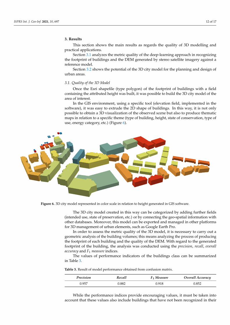
3.1. Quality of the 3D Model

Once the Esri shapefile (type polygon) of the footprint of buildings with a fieldcontaining the attributed height was built, it was possible to build the 3D city model of thearea of interest.

In the GIS environment, using a specific tool (elevation field, implemented in thesoftware), it was easy to extrude the 2D shape of buildings. In this way, it is not onlypossible to obtain a 3D visualization of the observed scene but also to produce thematicmaps in relation to a specific theme (type of building, height, state of conservation, type ofuse, energy category, etc.) (Figure 6).

ISPRS Int. J. Geo‐Inf. 2021, 10, x FOR PEER REVIEW  12  of  17  

 

The several steps described were performed using a ModelBuilder (a visual program‐

ming language) developed in ArcGIS Pro software. In this way, all processing was carried 

out in a controlled and automatic mode. 

3. Results 

This section shows the main results as regards the quality of 3D modelling and prac‐

tical applications. 

Section 3.1 analyzes the metric quality of the deep‐learning approach in recognizing 

the  footprint of buildings and  the DEM generated by stereo satellite  imagery against a 

reference model. 

Section 3.2 shows the potential of the 3D city model for the planning and design of 

urban areas. 

3.1. Quality of the 3D Model 

Once the Esri shapefile (type polygon) of the footprint of buildings with a field con‐

taining the attributed height was built, it was possible to build the 3D city model of the 

area of interest. 

In  the GIS environment, using a specific  tool  (elevation  field,  implemented  in  the 

software),  it was easy  to extrude  the 2D shape of buildings.  In  this way,  it  is not only 

possible to obtain a 3D visualization of the observed scene but also to produce thematic 

maps in relation to a specific theme (type of building, height, state of conservation, type 

of use, energy category, etc.) (Figure 6). 

 

Figure 6. 3D city model represented in color scale in relation to height generated in GIS software. 

The 3D city model created in this way can be categorized by adding further fields 

(intended use,  state of preservation, etc.) or by  connecting  the geo‐spatial  information 

with other databases. Moreover, this model can be exported and managed in other plat‐

forms for 3D management of urban elements, such as Google Earth Pro. 

In order to assess the metric quality of the 3D model, it is necessary to carry out a 

geometric analysis of the building volumes; this means analyzing the process of produc‐

ing the footprint of each building and the quality of the DEM. With regard to the gener‐

ated footprint of the building, the analysis was conducted using the precision, recall, over‐

all accuracy and F1 measure indices. 

The values of performance  indicators of the buildings class can be summarized  in 

Table 3. 

   

Figure 6. 3D city model represented in color scale in relation to height generated in GIS software.

The 3D city model created in this way can be categorized by adding further fields(intended use, state of preservation, etc.) or by connecting the geo-spatial information withother databases. Moreover, this model can be exported and managed in other platformsfor 3D management of urban elements, such as Google Earth Pro.

In order to assess the metric quality of the 3D model, it is necessary to carry out ageometric analysis of the building volumes; this means analyzing the process of producingthe footprint of each building and the quality of the DEM. With regard to the generatedfootprint of the building, the analysis was conducted using the precision, recall, overallaccuracy and F1 measure indices.

The values of performance indicators of the buildings class can be summarizedin Table 3.

Table 3. Result of model performance obtained from confusion matrix.

Precision Recall F1 Measure Overall Accuracy

0.957 0.882 0.918 0.852

While the performance indices provide encouraging values, it must be taken intoaccount that these values also include buildings that have not been recognized in their

ISPRS Int. J. Geo-Inf. 2021, 10, 697 13 of 17

true geometry; in other words, several buildings have been recognized as such, but in asimplified form that does not take into account their complexity, and several buildingshave been recognized as a single block.

With regard to the quality analysis of the height model generated by means of stereosatellite imagery, a comparison with another reference DEM was performed.

For example, DEMs generated by ALS systems are suitable for comparison. However,these DEMs are expensive to obtain and therefore not widely available on a regional andglobal scale.

For the study area, the best available DEM was the Space Shuttle Radar TopographyMission (SRTM). SRTM has collected, using synthetic aperture radar and interferometry, adigital elevation model of the Earth at 1 arc-second (30 meters) for over 80% of the Earth’ssurface [37,38]. It is available in 5◦ × 5◦ tiles, in geographic decimal degree (Latitude andLongitude) projection.

In order to use this DEM, the first step was to transform the DEM into UTM coordi-nates; this task was carried out using Global Mapper software.

In the mapping application, vertical accuracy is generally computed by the mean andVertical Root Mean Square Error (VRMSE). Taking into account a number (n) of groundcheck points evenly distributed over the study area and considering evi, the differencebetween the reference elevation at point i and DEM elevation at point i, it is possible towrite the following equation [39]:

VRMSE = ∓√

1n

n

∑i=1

e2vi (8)

For the study area, a mean value of 0.46 m and VRMSE of 5.98 m were achieved. Thesevalues are coherent with other works present in the literature [40,41]. In addition, it waspossible to build a histogram of errors where it was possible to note that most errors arearranged around the value zero, according to a Gaussian distribution. In particular, 83% ofthe points have an error of between −1 m and 1 m.

3.2. Contribution of the 3D Model in the Evaluation of a Project

In order to generate renders to support new designs using two different techniques,namely the use of decals and the import/realization of a new building design to verify itsappearance in the existing skyline, integration into BIM (Building Information Modeling)software was evaluated.

The import from GIS to CAD (Computer-Aided Design) required intermediate pro-cessing through the Meshlab software, which is an open-source system for processingand editing 3D triangular meshes; in this software, it was possible to import the modelgenerated by ArcScene (in the .wrl format) and exporting it, in turn, as a dxf (DrawingExchange Format) file format.

Once the file was imported into Autodesk Revit (enables design using parametricmodelling and drawing elements), it was possible to build a BIM model useful for planninga specific area. Indeed, BIM is the basis for digital transformation in the architecture,engineering and construction (AEC) sector. For example, it was possible to evaluate acoastal regeneration project within a 3D city model in LOD1, as shown in Figure 7.

ISPRS Int. J. Geo-Inf. 2021, 10, 697 14 of 17

ISPRS Int. J. Geo‐Inf. 2021, 10, x FOR PEER REVIEW  14  of  17  

 

interior; in this way, it is possible to quickly and accurately update the area concerned for 

the redevelopment of the city. 

 

(a) 

   

(b)  (c) 

Figure 7. Screen‐shot  in Revit software of coastal area  regeneration project within  the 3D city model  (a); examples of 

renderings of 3D views (b,c). 

4. Discussion and Conclusions 

The paper showed a novel method for the construction of a 3D city model starting 

from VHR stereo satellite imagery and based on the use of a deep‐learning approach for 

the identification of buildings’ footprints, the use of geomatics software for the construc‐

tion of the DEM and an algorithm implemented in the GIS environment for the extraction 

of the elevation of each building from the DEM. The innovative aspect of the proposed 

method with respect to what is present  in the literature concerns the  identification of a 

suitable workflow able to exploit the potential offered by deep‐learning algorithms for the 

construction of  the  footprint of buildings and  the availability of many  tools  in  the GIS 

environment that allows the construction of a 3D city model in a rather quick and effective 

way. To achieve this aim, the first step was to apply the pan‐sharpening technique to ob‐

tain a multispectral orthophoto of the area of interest at a high geometric resolution. 

Figure 7. Screen-shot in Revit software of coastal area regeneration project within the 3D city model (a); examples ofrenderings of 3D views (b,c).

BIM design is not limited to visual information or renderings but specifies the func-tionality and performance of each BIM object in the project or the elaborated buildinginterior; in this way, it is possible to quickly and accurately update the area concerned forthe redevelopment of the city.

4. Discussion and Conclusions

The paper showed a novel method for the construction of a 3D city model startingfrom VHR stereo satellite imagery and based on the use of a deep-learning approach for theidentification of buildings’ footprints, the use of geomatics software for the constructionof the DEM and an algorithm implemented in the GIS environment for the extractionof the elevation of each building from the DEM. The innovative aspect of the proposedmethod with respect to what is present in the literature concerns the identification of asuitable workflow able to exploit the potential offered by deep-learning algorithms forthe construction of the footprint of buildings and the availability of many tools in the GISenvironment that allows the construction of a 3D city model in a rather quick and effectiveway. To achieve this aim, the first step was to apply the pan-sharpening technique to obtaina multispectral orthophoto of the area of interest at a high geometric resolution.

ISPRS Int. J. Geo-Inf. 2021, 10, 697 15 of 17

From the comparison of the different pan-sharpening techniques, Brovey’s methodwas the one that provided the best results. This orthophoto was particularly useful for fur-ther processing, i.e., for the automatic classification of buildings. Indeed, the deep-learningapproach allowed, once the training data and an adequate model were created, the auto-matic recognition of the building footprints. This task was performed in semi-automaticallyby using ArcGIS Pro software. The performance indicators generated by the confusionmatrix showed very good quality of the classification level (overall accuracy equal to 0.852).These results are consistent with findings by other authors such as Pan et al. [42] who useda deep-learning approach and Worldview-2 satellite imagery on a dense urban area inthe Tianhe District of Guangzhou City (Southern China). In particular, very encouragingresults were obtained where the shape of buildings is geometrically linear and well defined.In the case where the structures are aggregates of several buildings and form more complexand articulated geometries, the deep-learning algorithms do not allow for an adequate re-construction of the footprint of the buildings. Compared to manual recognition of buildingfootprints, the automatic classification process showed some limitations in some urbanareas; this occurred due to the images (perspective) or to natural and anthropic elementspresent in the scene (vegetation, temporary structures, etc.).

With regard to the construction of the DEM, the approach implemented in Catalystsoftware made it possible to create the DEM from stereoscopic imagery in a quick, automaticand accurate way. In addition, the implementation of an algorithm for height extraction inthe GIS environment allowed the extraction of building heights from the DEM. Therefore,once the building geometry was constructed and a ‘height’ field was associated with eachbuilding, a 3D city model in LOD1 was obtained.

In addition, it is important to emphasize that the approach described in the paper(the use of deep learning for building the footprint, extracting the height from the DEMand building the 3D model) can also be used on images acquired from a UAV (UnmannedAerial Vehicle) or aircraft. Indeed, thanks to the recent developments of structure frommotion and multi-view stereo algorithms, it is possible to obtain both high-resolutionorthophotos and DEMs. Another possible and efficient way of using this approach isbased on using aerial hybrid sensors (color cameras and ALS), sensors capable of using thecamera to construct the orthophoto and ALS to generate a high-resolution DEM.

Finally, by combining the data produced by the national statistical institutes for build-ing surveys, concerning building permits and building extensions, and those from localauthorities concerning the new energy efficiency provisions, it is possible to thematize the3D model in order to identify buildings that have started or completed energy interven-tions, or those that would need such interventions. Further information to be thematizedin the 3D model could be that concerning the structural earthquake adaptation. Thesethemes would make it possible to produce maps for the definition of heat islands or seismicrisk areas. In this way, it is possible to construct a 3D city model that makes it possible toidentify the energy and structural state of each building and, more generally, of the entireurban environment according to the objectives of the 2030 Agenda on “sustainable citiesand communities” (goal 11).

Therefore, the possibility of realizing portions or entire urban areas, starting fromsatellite images and through the use of deep-learning algorithms, allows for digital re-construction of a highly performant 3D model to support professionals, companies andpublic administrations engaged in the planning and design sector [43]. The interoperabilityof these models, with the most common BIM software [44], not only increases the levelof detail of the design but also allows one, by combining a series of heterogeneous data(technical data, geospatial positioning, point clouds, digital images, etc.), to perform andshare analyses on 3D and 4D models during the different phases of the planning cycle at alarge and medium scale. Hence, the fields of application of the 3D city model are manifold;in fact, a further application concerns the cadastral field [45] where 3D digital models, suchas BIM and 3D GIS, could be utilized for the accurate identification of property units, betterrepresentation of cadastral boundaries and detailed visualization of complex buildings.

ISPRS Int. J. Geo-Inf. 2021, 10, 697 16 of 17

Author Contributions: Conceptualization, Massimiliano Pepe, Domenica Costantino, VincenzoSaverio Alfio, Gabriele Vozza and Elena Cartellino; methodology, Massimiliano Pepe, DomenicaCostantino, Vincenzo Saverio Alfio, Gabriele Vozza and Elena Cartellino; software, MassimilianoPepe, Domenica Costantino, Vincenzo Saverio Alfio, Gabriele Vozza and Elena Cartellino; vali-dation, Massimiliano Pepe, Domenica Costantino, Vincenzo Saverio Alfio, Gabriele Vozza andElena Cartellino; formal analysis, Massimiliano Pepe, Domenica Costantino, Vincenzo Saverio Al-fio, Gabriele Vozza and Elena Cartellino; investigation, Massimiliano Pepe, Domenica Costantino,Vincenzo Saverio Alfio, Gabriele Vozza and Elena Cartellino; resources, Massimiliano Pepe andDomenica Costantino; data curation, Massimiliano Pepe, Domenica Costantino, Vincenzo SaverioAlfio, Gabriele Vozza and Elena Cartellino; writing—original draft preparation, Massimiliano Pepe,Domenica Costantino, Vincenzo Saverio Alfio, Gabriele Vozza and Elena Cartellino; writing—reviewand editing, Massimiliano Pepe, Domenica Costantino, Vincenzo Saverio Alfio, Gabriele Vozza andElena Cartellino. All authors have read and agreed to the published version of the manuscript.

Funding: This research received no external funding.

Institutional Review Board Statement: Not applicable.

Informed Consent Statement: Not applicable.

Data Availability Statement: Not applicable.

Conflicts of Interest: The authors declare no conflict of interest.

References1. Jovanovic, D.; Milovanov, S.; Ruskovski, I.; Govedarica, M.; Sladic, D.; Radulovic, A.; Pajic, V. Building Virtual 3D City Model

for Smart Cities Applications: A Case Study on Campus Area of the University of Novi Sad. ISPRS Int. J. Geo-Inf. 2020, 9, 476.[CrossRef]

2. Gröger, G.; Plümer, L. CityGML—Interoperable semantic 3D city models. ISPRS Int. J. Geo-Inf. 2012, 71, 12–33. [CrossRef]3. Pepe, M.; Costantino, D.; Alfio, V.S.; Angelini, M.G.; Restuccia Garofalo, A. A CityGML Multiscale Approach for the Conservation

and Management of Cultural Heritage: The Case Study of the Old Town of Taranto (Italy). ISPRS Int. J. Geo-Inf. 2020, 9, 449.[CrossRef]

4. Kutzner, T.; Chaturvedi, K.; Kolbe, T.H. CityGML 3.0: New functions open up new applications. PFG–J. Photogramm. Remote Sens.Geoinf. Sci. 2020, 88, 43–61. [CrossRef]

5. Zhang, K.; Yan, J.; Chen, S.C. Automatic construction of building footprints from airborne LIDAR data. IEEE Trans. Geosci. RemoteSens. 2006, 44, 2523–2533. [CrossRef]

6. Rubinowicz, P. Generation of CityGML LoD1 City Models Using BDOT10k and LiDAR Data. Space Form 2017, 31, 61–74.7. Ortega, S.; Santana, J.M.; Wendel, J.; Trujillo, A.; Murshed, S.M. Generating 3D city models from open LiDAR point clouds:

Advancing towards smart city applications. In Open Source Geospatial Science for Urban Studies; Springer: Cham, Switzerland, 2021;pp. 97–116.

8. Pepe, M.; Fregonese, L.; Crocetto, N. Use of SfM-MVS approach to nadir and oblique images generated throught aerial camerasto build 2.5 D map and 3D models in urban areas. Geocarto Int. 2019, 1–22. [CrossRef]

9. Parente, C.; Pepe, M. Bathymetry from worldview-3 satellite data using radiometric band ratio. Acta Polytech. 2018, 58, 109–117.[CrossRef]

10. Daliakopoulos, I.N.; Tsanis, I.K. A SIFT-Based DEM Extraction Approach Using GEOEYE-1 Satellite Stereo Pairs. Sensors 2019, 19,1123. [CrossRef]

11. Proietti, C.; Coltelli, M.; Marsella, M.; Martino, M.; Scifoni, S.; Giannone, F. Towards a satellite-based approach to measureeruptive volumes at Mt. Etna using Pleiades datasets. Bull. Volcanol. 2020, 82, 1–15. [CrossRef]

12. Zhong, C.; Liu, Y.; Gao, P.; Chen, W.; Li, H.; Hou, Y.; Ma, H. Landslide mapping with remote sensing: Challenges and opportunities.Int. J. Remote Sens. 2020, 41, 1555–1581. [CrossRef]

13. Hirschmuller, H. Stereo processing by semiglobal matching and mutual information. IEEE Trans. Pattern Anal. Mach. Intell. 2007,30, 328–341. [CrossRef] [PubMed]

14. Rajpriya, N.R.; Vyas, A.; Sharma, S.A. Generation of 3D Model for Urban area using Ikonos and Cartosat-1 Satellite Imagerieswith RS and GIS Techniques. Int. Arch. Photogramm. Remote Sens. Spat. Inf. Sci. 2014, 40, 899. [CrossRef]

15. Partovi, T.; Fraundorfer, F.; Bahmanyar, R.; Huang, H.; Reinartz, P. Automatic 3-D building model reconstruction from very highresolution stereo satellite imagery. Remote Sens. 2019, 11, 1660. [CrossRef]

16. Kumar, M.; Bhardwaj, A. Building Extraction from Very High Resolution Stereo Satellite Images using OBIA and TopographicInformation. Environ. Sci. Proc. 2020, 5, 1.

17. Yuan, J. Learning building extraction in aerial scenes with convolutional networks. IEEE Trans. Pattern Anal. Mach. Intell. 2017, 40,2793–2798. [CrossRef] [PubMed]

ISPRS Int. J. Geo-Inf. 2021, 10, 697 17 of 17

18. Xu, Y.; Wu, L.; Xie, Z.; Chen, Z. Building extraction in very high resolution remote sensing imagery using deep learning andguided filters. Remote Sens. 2018, 10, 144. [CrossRef]

19. Tripodi, S.; Duan, L.; Poujade, V.; Trastour, F.; Bauchet, J.P.; Laurore, L.; Tarabalka, Y. Operational Pipeline for Large-Scale3D Reconstruction of Buildings from Satellite Images. In IGARSS 2020–2020 IEEE International Geoscience and Remote SensingSymposium; IEEE: Waikoloa, HI, USA, 2020; pp. 445–448.

20. Rastogi, K.; Bodani, P.; Sharma, S.A. Automatic building footprint extraction from very high-resolution imagery using deeplearning techniques. Geocarto Int. 2020, 1–13. [CrossRef]

21. Li, H.; Jing, L.; Tang, Y. Assessment of pansharpening methods applied to WorldView-2 imagery fusion. Sensors 2017, 17, 89.[CrossRef]

22. Kocaman, S.; Zhang, L.; Gruen, A.; Poli, D. 3D city modeling from high-resolution satellite images. International Archives of thePhotogrammetry. Remote Sens. Spat. Inf. Sci. 2006, 36 (1/W41). [CrossRef]

23. Duan, L.; Lafarge, F. Towards Large-Scale City Reconstruction from Satellites. In Computer Vision–ECCV; Leibe, B., Matas, J., Sebe,N., Welling, M., Eds.; Lecture Notes in Computer Science; Springer: Cham, Switzerland, 2016; Volume 9909. [CrossRef]

24. Zhao, L.; Liu, Y.; Men, C.; Men, Y. Double Propagation Stereo Matching for Urban 3-D Reconstruction from Satellite Imagery.IEEE Trans. Geosci. Remote Sens. 2021, 1–17.

25. Parente, C.; Pepe, M. Influence of the weights in IHS and Brovey methods for pan-sharpening WorldView-3 satellite images. Int.J. Eng. Technol. 2017, 6, 71–77. [CrossRef]

26. Vivone, G.; Alparone, L.; Chanussot, J.; Dalla Mura, M.; Garzelli, A.; Licciardi, G.A.; Wald, L. A critical comparison amongpansharpening algorithms. IEEE Trans. Geosci. Remote Sens. 2015, 53, 2565–2586. [CrossRef]

27. Baiocchi, V.; Bianchi, A.; Maddaluno, C.; Vidale, M. Pansharpening techniques to detect mass monument damaging in Iraq. Int.Arch. Photogramm. Remote Sens. Spat. Inf. Sci. 2017, 42, 121–126. [CrossRef]

28. Chen, S.; Zhang, R.; Su, H.; Tian, J.; Xia, J. Scaling-up transformation of multisensor images with multiple resolutions. Sensors2009, 9, 1370–1381. [CrossRef] [PubMed]

29. Hegde, G.P.; Hegde, N.; Muralikrishna, V.D.I. Measurement of quality preservation of pan-sharpened image. Int. J. Eng. Res. Dev.2012, 2, 12–17.

30. Lillo-Saavedra, M.; Gonzalo, C. Spectral or spatial quality for fused satellite imagery? A trade-off solution using the wavelet átrous algorithm. Int. J. Remote Sens. 2006, 27, 1453–1464. [CrossRef]

31. Wald, L. Quality of high resolution synthesized images: Is there a simple criterion? In Proceedings of the International ConferenceFusion of Earth Data, Nice, France, 26–28 January 2000; Volume 1, pp. 99–105.

32. Pepe, M.; Parente, C. Burned area recognition by change detection analysis using images derived from Sentinel-2 satellite: Thecase study of Sorrento Peninsula, Italy. J. Appl. Eng. Sci. 2018, 16, 225–232. [CrossRef]

33. Yekeen, S.T.; Balogun, A.L.; Yusof, K.B.W. A novel deep learning instance segmentation model for automated marine oil spilldetection. ISPRS J. Photogramm. Remote Sens. 2020, 167, 190–200. [CrossRef]

34. Croce, V.; Caroti, G.; De Luca, L.; Jacquot, K.; Piemonte, A.; Véron, P. From the Semantic Point Cloud to Heritage-BuildingInformation Modeling: A Semiautomatic Approach Exploiting Machine Learning. Remote Sens. 2021, 13, 461. [CrossRef]

35. O’Rourke, J. Computational Geometry in C, 2nd ed.; Cambridge University Press: Cambridge, UK, 1998.36. Chazelle, B. Triangulating a simple polygon in linear time. Discret. Comput. Geom. 1991, 6, 485–524. [CrossRef]37. Gribov, A. Searching for a compressed polyline with a minimum number of vertices. In 2017 14th IAPR International Conference on

Document Analysis and Recognition; IEEE: Tokyo, Japan, 2017; pp. 13–14.38. Farr, T.G.; Kobrick, M. Shuttle radar topography mission produces a wealth of data. Trans. Am. Geophys. Union 2000, 81, 583–585.

[CrossRef]39. Mukul, M.; Srivastava, V.; Mukul, M. Analysis of the accuracy of Shuttle Radar Topography Mission (SRTM) height models using

International Global Navigation Satellite System Service (IGS) Network. J. Earth Syst. Sci. 2015, 124, 1343–1357. [CrossRef]40. Elkhrachy, I. Vertical accuracy assessment for SRTM and ASTER Digital Elevation Models: A case study of Najran city, Saudi

Arabia. Ain Shams Eng. J. 2018, 9, 1807–1817. [CrossRef]41. Misra, P.; Avtar, R.; Takeuchi, W. Comparison of digital building height models extracted from AW3D, TanDEM-X, ASTER, and

SRTM digital surface models over Yangon City. Remote Sens. 2008, 10, 2008. [CrossRef]42. Pan, Z.; Xu, J.; Guo, Y.; Hu, Y.; Wang, G. Deep learning segmentation and classification for urban village using a worldview

satellite image based on U-Net. Remote Sens. 2020, 12, 1574. [CrossRef]43. Leal Filho, W.; Azul, A.M.; Brandli, L.; Özuyar, P.G.; Wall, T. (Eds.) Sustainable Cities and Communities; Springer: Berlin/Heidelberg,

Germany, 2019.44. Jetlund, K.; Onstein, E.; Huang, L. IFC schemas in ISO/TC 211 compliant UML for improved interoperability between BIM and

GIS. ISPRS Int. J. Geo-Inf. 2020, 9, 278. [CrossRef]45. Sun, J.; Mi, S.; Olsson, P.O.; Paulsson, J.; Harrie, L. Utilizing BIM and GIS for Representation and Visualization of 3D Cadastre.

ISPRS Int. J. Geo-Inf. 2019, 8, 503. [CrossRef]