Available online at www.sciencedirect.com

Statistics & Probability Letters 67 (2004) 321–330

A note on the estimation of the initial numberof susceptible individuals in the general

epidemic model

Richard M. Hugginsa, Paul S.F. Yipb;∗, Eric H.Y. Laub

aDepartment of Statistical Science, La Trobe University, Bundoora 3083, AustraliabDepartment of Statistics and Actuarial Science, The University of Hong Kong, Hong Kong

Abstract

Traditional inference for epidemic models depends on knowledge of the initial number of susceptibleindividuals. However, this may be di/cult to obtain in practice. In this short note we show that it is possibleto use data from a major epidemic to estimate the number of individuals initially susceptible to a disease andan approximate asymptotic variance is derived. The results are con3rmed in simulations of major epidemics.An application to a data set on smallpox is given.c© 2004 Elsevier B.V. All rights reserved.

Keywords: Epidemic; Population size estimation; Susceptibles

1. Introduction

The estimation of the size of a population is a common problem in many scienti3c disciplines,for example, in ecology and software engineering (Pollock, 2000; Huggins, 1989; Blumenthal andMarcus, 1975; Sanathanan, 1977; van Pul, 1992; Andersen et al., 1993; Yip, 1995; Yip et al., 1996;Chao et al., 2001). In epidemiological studies, not all individuals that are susceptible to a certaindisease will be infected in an outbreak of the disease and we encounter the related problem ofestimating the initial number of individuals that are susceptible to a disease would be of interest.The number of initially susceptible individuals is required to estimate the model parameters that forexample may be used to estimate the probability of a major epidemic for the disease of interest. Theability to estimate the number of susceptible individuals at an early stage in an epidemic places anupper bound on the size of the epidemic to aid in management strategies. Moreover, if the number

∗ Corresponding author. Tel.: +852-2859-1989; fax: +852-2858-9041.E-mail address: sfpyip@hku.hk (S.F. Yip).

0167-7152/$ - see front matter c© 2004 Elsevier B.V. All rights reserved.doi:10.1016/j.spl.2002.02.001

322 R.M. Huggins et al. / Statistics & Probability Letters 67 (2004) 321–330

of initially uninfected individuals is known, then by comparing this number with the estimatednumber of initially susceptible individuals, the methods presented here have the potential to determineif there are individuals in the population with either a natural immunity to the disease or are forsome reasons not exposed to the disease.

For example, in the study of the AIDS epidemic, HIV positive cases are recorded but the size ofthe group at risk is usually unknown. Estimation of the initial number of susceptible individuals inan epidemic model can be seen as related to a removal process in an ecological removal experiment(Seber, 1982; Huggins and Yip, 1997). However, the features of high dependency between individualsin epidemic process makes the estimation problem di/cult and challenging (Becker and Yip, 1989;Becker and Cui, 1998; Yip and Chen, 1998). Here we show that if an epidemic is fully observedin that we know the infection and removal times of the infected individuals then estimation of theinitial number of susceptibles is possible. We apply the procedure with reference to the Abakalikismallpox data in Nigeria that has been previously considered by other authors.

2. Notation

In this paper we consider the Rida (1991) parameterization of the general epidemic model ofBailey (1975, p. 82), which describes the spread of a Susceptible-Infected-Removal (SIR) infectiousdisease in a population of homogeneous individuals who mix uniformly. Our interest is in thesituation where the initial number of susceptibles is unknown and is regarded as a model parameter.

Suppose the epidemic is observed for a time �. For 06 t6 �, let: S(t) denote the number ofsusceptibles present at time t: N (t) denote the number of individuals infected up to and includingtime t, including the initial infectives: I(t) denote the number of infectives present at time t: R(t)denote the number of infected individuals removed by quarantine, death or being cured of the disease,up to and including time t: i0 denote the initial number of infectives: denote the initial numberof susceptibles: denote the infection rate: � denote the removal rate: Ft denote the �−algebragenerated by the history {S(u); I(u); 06 u6 t}. Following the parameterization of Rida (1991), wesuppose that given S(t) and I(t) the probability a susceptible is infected in a small time interval(t; t + dt) is

S(t)I(t) dt + o( dt);

so that

Pr{dN (t) = 1; dR(t) = 0|Ft}= S(t)I(t) dt + o(dt); (1)

Pr{dN (t) = 0; dR(t) = 1|Ft}= �I(t) dt + o(dt); (2)

Pr{dN (t) = 0; dR(t) = 0|Ft}=1− S(t)I(t) dt − �I(t) + o(dt):

Note that I(t) = S(t)− R(t).We are interested in the situation where the numbers of susceptibles S(t) are not observable.

However, the infection times of the individuals that were infected in [0; �] are supposed to beobservable. Our inferences are based on the observations on the infection times of these individuals

R.M. Huggins et al. / Statistics & Probability Letters 67 (2004) 321–330 323

and observations on when their infectivity ceased due to removal. That is, we observe S�(t)=N (�)−N (t−), the number of individuals that were infected in [0; �] that were still susceptible at time t.

3. The estimator

The full likelihood requires knowledge of the number of infectives I(t) and susceptibles S(t) ateach t, 06 t6 �. We observe S�(t) rather than S(t). Now,

M (t) = (N (t)− i0)−∫ t

0

S(u)I(u) du (3)

is a zero mean martingale. Note that the total number of susceptibles at u is just S�(u) plus thenumber of susceptibles not infected by �, or S(u) = S�(u) + (− N (�) + i0). Substituting this in (3)yields

(N (t)− i0)−

{∫ t

0S�(u)I(u) ds+ (− N (�) + i0)

∫ t

0I(u) du

}(4)

is also a martingale. Hence, the martingale estimating equation estimator of is

=(N (�)− i0)∫ �

0 S�(u)I(u) ds+ (− N (�) + i0)∫ �0 I(u) du

: (5)

Let K1=∫ t0 S�(u)I(u) du and K2=

∫ �0 I(u) du. Then we may write =((N (�)− i0))=(K1+(−N (�)+

i0)K2) when is unknown. Let �(; ) = 1− exp (−K2=) be the probability a randomly selectedsusceptible is infected in [0; �] given K2. Then, as N (�)− i0 ∼ Bin(;�(; )), (N (�)− i0)−�(; )has zero mean, and the method of moments suggests that we estimate by the solution of theestimating equation

(N (�)− i0)− {1− exp

( −K2(N (�)− i0)K1 + (− N (�) + i0)K2

)}= 0: (6)

The resulting estimator may then be found numerically.

4. Properties of the estimator

4.1. Consistency

Let

=(N (�)− i0)

(K1 + (− N (�) + i0)K2)=

(N (�)− i0)∫ �0 S(u)I(u) du

be the estimated value of if were known. Then, as this is the standard estimator when thenumber of susceptibles is observed, it is known that in the case of a major outbreak

p→ as→ ∞ (Rida, 1991; Britton, 1998; Yip and Chen, 1998). De3ne g()=−1(N (�)− i0)−�(; ) and

324 R.M. Huggins et al. / Statistics & Probability Letters 67 (2004) 321–330

let =(�(; ))−1(N (�)− i0) be the solution of g()=0. We have noted above that N (�)− i0 has abinomial distribution so that −1(− ) p→0 and −1=2(− ) d→N (0; (1−�(; ))=�(; )). Next, as

K1 + (− N (�) + i0)K2

K1 + (− N (�) + i0)K2− 1 =

K2(− )K1 + (− N (�) + i0)K2

;

we have

�() = 1− exp( −K2(N (�)− i0)K1 + (− N (�) + i0)K2

)

=1− exp

{− K2

(K2(− )

K1 + (− N (�) + i0)K2+ 1)}

:

Hence,

�(; )−�()

= exp

{− K2

(K2(− )

K1 + (− N (�) + i0)K2+ 1)}

− exp(− K2

)

=exp{− K2

}[exp

{− K2

K2(− )

K1 + (− N (�) + i0)K2− K2

+K2

}− 1

]

≈ exp{− K2

}[exp

{− K2

K2(− )

K1 + (− N (�) + i0)K2

}− 1

]: (7)

Now, under mild conditions, −1(−) p→0, −1K2 converges in probability, as does −1(−N (�)+i0)and −1−1K1. Hence, (7) converges in probability to zero.Next,

N (�)− i0�(; )

≈ N (�)− i0�(; )

− N (�)− i0�2(; )

(�()−�(; ));

so that

≈ − (�()−�(; ))�(; )

= {1−

(�()�(; )

− 1)}

= (2− �()

�(; )

)and arguing as in (7) and as −1=2 converges in distribution, we see that −1=2(− ) p→0 and henceconclude that −1=2(− ) converges in distribution.

R.M. Huggins et al. / Statistics & Probability Letters 67 (2004) 321–330 325

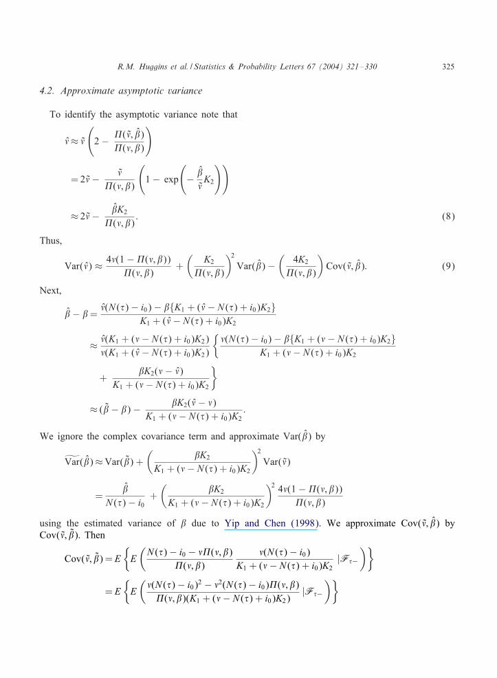
4.2. Approximate asymptotic variance

To identify the asymptotic variance note that

≈ (2− �(; )

�(; )

)

=2− �(; )

(1− exp

(− K2

))

≈ 2− K2

�(; ): (8)

Thus,

Var() ≈ 4(1−�(; ))�(; )

+(

K2

�(; )

)2Var()−

(4K2

�(; )

)Cov(; ): (9)

Next,

− = (N (�)− i0)− {K1 + (− N (�) + i0)K2}K1 + (− N (�) + i0)K2

≈ (K1 + (− N (�) + i0)K2)(K1 + (− N (�) + i0)K2)

{(N (�)− i0)− {K1 + (− N (�) + i0)K2}

K1 + (− N (�) + i0)K2

+K2(− )

K1 + (− N (�) + i0)K2

}≈ ( − )− K2(− )

K1 + (− N (�) + i0)K2:

We ignore the complex covariance term and approximate Var() by

Var()≈Var() +(

K2

K1 + (− N (�) + i0)K2

)2Var()

=

N (�)− i0 +(

K2

K1 + (− N (�) + i0)K2

)2 4(1−�(; ))�(; )

using the estimated variance of due to Yip and Chen (1998). We approximate Cov(; ) byCov(; ). Then

Cov(; ) = E{E(N (�)− i0 − �(; )

�(; )(N (�)− i0)

K1 + (− N (�) + i0)K2|F�−

)}

= E{E((N (�)− i0)2 − 2(N (�)− i0)�(; )�(; )(K1 + (− N (�) + i0)K2)

|F�−)}

326 R.M. Huggins et al. / Statistics & Probability Letters 67 (2004) 321–330

= E{

2(1−�(; ))K1 + (− N (�) + i0)K2

}est=

2(1−�(; ))K1 + (− N (�) + i0)K2

;

as E{(N (�)− i0)2|K2}= �(; ){1−�(; )}+ 2�(; )2. Substitution of these quantities in (9)results in an approximate asymptotically conservative estimate of the variance of the estimatednumber of initially susceptible individuals. From this estimate we may construct approximate nominal95% con3dence intervals of the form ± 1:96s:e:().

Remark. Estimation of the Cov(; ) term in Var() by the obvious approximate estimator arisingfrom (8),

22(1−�(; ))K1 + (− N (�) + i0)K2

− K2

�(; )

(N (�)− i0)

did not result in an improved performance in the simulations. We therefore retained the simplerapproximation.

5. Simulations

We considered populations of = 100, = 250, and = 1000, and = 5000 susceptibles withi0 = 5 introductory cases. We took � = 1 and = 1:5 and 1.3. As the results are conditional on amajor epidemic we only considered simulated epidemics where more than 20% of the individualswere infected and for = 1:3 we also considered simulated epidemics where more than 40% ofthe individuals were infected. For each combination of parameters, 1000 epidemics were simulated.The value of was used as the starting value. A small number of simulations where the estimatescould not be computed were omitted and new epidemics simulated. The epidemics were generatedby simulating 2 exponential random variables, the 3rst, T1 with rate S(t)I(t)= and the second T2with rate �I(t). We took T = T1 ∧ T2 and if T1¡T2 a new infection was recorded and otherwise aremoval was recorded. The results are reported in Table 1. These simulation results suggest that aslong as the disease is reasonably infective the estimator is performing well. The estimator exhibitednegative bias for small population sizes. For = 1:3 with a smaller infected proportion it seemsthat the variance was also underestimated. In the simulations with = 1:3 and with a minimum of40% infection to de3ne a major epidemic, it is seen that the bias can be remedied by increasing thepercentage of the initial number of susceptibles required to be infected to de3ne a major epidemicbut there is still some underestimation of the variance.

6. A smallpox example

We illustrate the procedure on the Abakaliki smallpox data in Nigeria. Becker (1989) gives thevalues of the times of the infections, as well as the number of infectious individuals on eachday during the epidemic, under the assumption that the latent period has duration of 13 days and

R.M. Huggins et al. / Statistics & Probability Letters 67 (2004) 321–330 327

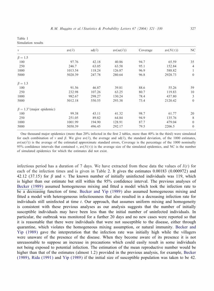
Table 1Simulation results

av() sd() av(se()) Coverage av(N (�)) NC

= 1:5100 97.76 42.18 40.86 94.7 65.59 35250 246.7 63.05 63.58 95.1 152.84 41000 1013.54 118.24 126.87 96.9 588.82 15000 5020.39 247.78 280.64 96.8 2928.73 0

= 1:3100 91.56 46.87 39.81 88.6 55.26 59250 232.98 107.26 63.25 80.7 119.83 101000 982.67 298.27 130.24 78.4 437.80 35000 5012.18 550.55 293.38 73.4 2120.42 0

= 1:3∗(major epidemic)100 99.38 43.11 41.32 98.7 61.77 20250 251.05 89.82 64.84 94.9 135.76 81000 1001.99 194.90 128.91 87.7 479.04 05000 5050.39 496.45 292.17 79.5 2206.5 0

One thousand major epidemics (more than 20% infected in the 3rst 2 tables, more than 40% in the third) were simulatedfor each combination of and . We give av(), the average and sd(), the standard deviation, of the 1000 estimates,av(se()) is the average of the estimated approximate standard errors, Coverage is the percentage of the 1000 nominally95% con3dence intervals that contained , av(N (�)) is the average size of the simulated epidemics, and NC is the numberof simulated epidemics for which the estimates did not exist.

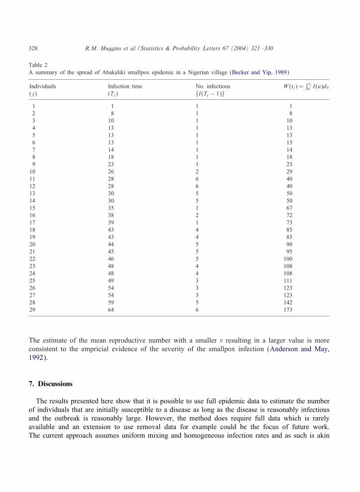
infectious period has a duration of 7 days. We have extracted from these data the values of I(t) foreach of the infection times and is given in Table 2. It gives the estimates 0.00183 (0.000972) and42.12 (37.15) for and . The known number of initially uninfected individuals was 119, whichis higher than our estimate but still within the 95% con3dence interval. The previous analyses ofBecker (1989) assumed homogeneous mixing and 3tted a model which took the infection rate tobe a decreasing function of time. Becker and Yip (1989) also assumed homogeneous mixing and3tted a model with heterogeneous infectiousness that also resulted in a decreasing infection rate forindividuals still uninfected at time t. Our approach, that assumes uniform mixing and homogeneityis consistent with these previous analyses as our analysis suggests that the number of initiallysusceptible individuals may have been less than the initial number of uninfected individuals. Inparticular, the outbreak was monitored for a further 20 days and no new cases were reported so thatit is reasonable that there were individuals that were not susceptible to the disease, either throughquarantine, which violates the homogeneous mixing assumption, or natural immunity. Becker andYip (1989) gave the interpretation that the infection rate was initially high while the villagerswere unaware of the presence of the disease. When they become aware of its presence it is notunreasonable to suppose an increase in precautions which could easily result in some individualsnot being exposed to potential infection. The estimation of the mean reproductive number would behigher than that of the estimates (almost 1.2) provided in the previous analysis, for example, Becker(1989), Rida (1991) and Yip (1989) if the initial size of susceptible population was taken to be 42.

328 R.M. Huggins et al. / Statistics & Probability Letters 67 (2004) 321–330

Table 2A summary of the spread of Abakaliki smallpox epidemic in a Nigerian village (Becker and Yip, 1989)

Individuals Infection time No. infectious W (tj) =∫ tj0 I(u)d0

(j) (Tj) {I(Tj − 1)}1 1 1 12 8 1 83 10 1 104 13 1 135 13 1 136 13 1 137 14 1 148 18 1 189 23 1 2310 26 2 2911 28 6 4012 28 6 4013 30 5 5014 30 5 5015 35 1 6716 38 2 7217 39 1 7318 43 4 8519 43 4 8520 44 5 9021 45 5 9522 46 5 10023 48 4 10824 48 4 10825 49 3 11126 54 3 12327 54 3 12328 59 5 14229 64 6 173

The estimate of the mean reproductive number with a smaller resulting in a larger value is moreconsistent to the empricial evidence of the severity of the smallpox infection (Anderson and May,1992).

7. Discussions

The results presented here show that it is possible to use full epidemic data to estimate the numberof individuals that are initially susceptible to a disease as long as the disease is reasonably infectiousand the outbreak is reasonably large. However, the method does require full data which is rarelyavailable and an extension to use removal data for example could be the focus of future work.The current approach assumes uniform mixing and homogeneous infection rates and as such is akin

R.M. Huggins et al. / Statistics & Probability Letters 67 (2004) 321–330 329

to the homogeneous capture probability model M0 (Otis et al., 1978) applied in capture–recapturestudies to estimate the size of an animal population. As in the capture–recapture case clearly thereis scope to extend the present approach to more complex models.

The approximation to the asymptotic variance was shown in the simulations to be conservative ifthe initial number of susceptible individuals is large and re3nement of this expression may also beworthwhile. That the estimator breaks down when a disease is not highly infectious and the numberof susceptibles is small to moderately large is not surprising as we are conditioning on a majorepidemic, and indeed the estimates of in these simulations were positively biased. Intuitively therewould seem to be something of an identi3ability problem arising from conditioning on a majorepidemic for a disease that is not highly infectious and the bias in our simulation results seem tobe a consequence of this. This may be the case in the example where it is not clear there is amajor outbreak and suggests that in these circumstances the estimator be taken as a lower bound.However, our analysis of the example does appear to be consistent with previous analyses thatyield an estimate of the infectiousness that decreases with time. Of more concern is the bias in theestimated variance when = 1:3 which suggests the approximations in computing the variances arenot universally small.

The stated properties of our estimator requires a major epidemic. There is some vagueness in theliterature concerning the de3nition of a major epidemic as it relates to the limit of the total size ofan epidemic Nn as the initial number of susceptible individuals n→ ∞ being in3nite (Rida, 1991).That is, some non-zero proportion of the population is infected. However, in observing a singleepidemic on a 3nite population whether or not a major epidemic has occurred may not be apparent.The unconditional probability of a major epidemic can be estimated using model parameters (Rida,1991; Yip, 1989; Ball, 1983) but we require the conditional probability of a major epidemic giventhe observed epidemic which is a more di/cult quantity to determine.

Acknowledgements

The authors would like to thank the referees’ comments and the work is supported by a CRCGof the University of Hong Kong and a RGC Grant.

References

Anderson, R.M., May, R.T., 1992. Infectious Diseases of Humans. OUP, Oxford.Andersen, P.K., Borgan, Q., Gill, R.D., Keiding, N., 1993. Statistical Models Based on Counting Processes. Springer,

New York.Bailey, N.T.J., 1975. The Mathematical Theory of Infectious Disease. Gri/n, London.Ball, F.G., 1983. The threshold behavior of epidemic models. J. Appl. Probab. 20, 227–241.Becker, N.G., 1989. Analysis of Infectious Disease Data. Chapman & Hall, London.Becker, N.G., Cui, J., 1998. Statistical studies of AIDS and HIV. Encyclopedia of Biostatistics. Wiley, UK, pp. 117–123.Becker, N.G., Yip, P., 1989. Analysis of variations in an infection rate. Austral. J. Statist. 31, 42–52.Blumenthal, S., Marcus, R., 1975. Estimating population size with exponential failure. J. Amer. Statist. Assoc. 70,

913–922.Britton, T., 1998. Estimation in multitype epidemics. J. Roy. Statist. Soc. 60, 663–679.Chao, A., Tsay, P.K., Lin, S.H., Shau, W.Y., Chao, D.Y., 2001. The application of capture–recapture models to

epidemiological data. Statist. Med. 20, 3123–3157.

330 R.M. Huggins et al. / Statistics & Probability Letters 67 (2004) 321–330

Huggins, R.M., 1989. On the statistical analysis of capture experiments. Biometrika 76, 133–140.Huggins, R.M., Yip, P.S.F., 1997. Statistical analysis of removal experiments with the use of auxiliary variables. Statistica

Sinica 7, 705–712.Otis, D.L., Burnham, K.P., White, G.C., Anderson, D.R., 1978. Statistical inference from capture data on closed animal

populations. Wildlife Monograph, Vol. 62. The Wildlife Society, Washington, DC.Pollock, K.H., 2000. Capture–recapture models. J. Amer. Statist. Assoc. 95, 293–296.Rida, W.N., 1991. Asymptotic properties of some estimators for the infection rate in the general stochastic epidemic

model. J. Roy. Statist. Soc. B 53, 269–283.Sanathanan, L., 1977. Estimating the size of a truncated sample. J. Amer. Statist. Assoc. 72, 669–672.Seber, G.A.F., 1982. The Estimation of Animal Abundance and Related Parameters, 2nd Edition. Macmillan, New York.van Pul, M.C., 1992. Asymptotic properties of a class of statistical models in software reliability. Scand. J. Statist. 19,

235–253.Yip, P.S.F., 1989. Estimation for initial relative infection rate for a stochastic epidemic model. Theoret. Population Biol.

36, 202–213.Yip, P.S.F., 1995. Estimating the number of errors in a system—using a martingale approach. IEEE Trans. Reliability 44,

322–326.Yip, P.S.F., Chen, Q.Z., 1998. Statistical Inference for a multi-type epidemic model. J. Statist. Plann. Inference 71,

229–244.Yip, P.S.F., Huggins, R.M., Lin, D.Y., 1996. Inference for capture–recapture experiments in continuous time with variable

capture rates. Biometrika 83, 477–483.