Original Paper

FluBreaks: Early Epidemic Detection from Google Flu Trends

Fahad Pervaiz, BS; Mansoor Pervaiz, BS; Nabeel Abdur Rehman, BS(Current); Umar Saif, BS, PhD, PostdocSchool of Science and Engineering, Computer Science Department, Lahore University of Management Sciences, Lahore, Pakistan

Corresponding Author:Fahad Pervaiz, BSSchool of Science and EngineeringComputer Science DepartmentLahore University of Management SciencesOpposite Sector-U, D.H.A.Lahore, 54792PakistanPhone: 92 333 443 8347Fax: 92 42 3560 8303Email: fahadp@lums.edu.pk

Abstract

Background: The Google Flu Trends service was launched in 2008 to track changes in the volume of online search queriesrelated to flu-like symptoms. Over the last few years, the trend data produced by this service has shown a consistent relationshipwith the actual number of flu reports collected by the US Centers for Disease Control and Prevention (CDC), often identifyingincreases in flu cases weeks in advance of CDC records. However, contrary to popular belief, Google Flu Trends is not an earlyepidemic detection system. Instead, it is designed as a baseline indicator of the trend, or changes, in the number of disease cases.

Objective: To evaluate whether these trends can be used as a basis for an early warning system for epidemics.

Methods: We present the first detailed algorithmic analysis of how Google Flu Trends can be used as a basis for building afully automated system for early warning of epidemics in advance of methods used by the CDC. Based on our work, we presenta novel early epidemic detection system, called FluBreaks (dritte.org/flubreaks), based on Google Flu Trends data. We comparedthe accuracy and practicality of three types of algorithms: normal distribution algorithms, Poisson distribution algorithms, andnegative binomial distribution algorithms. We explored the relative merits of these methods, and related our findings to changesin Internet penetration and population size for the regions in Google Flu Trends providing data.

Results: Across our performance metrics of percentage true-positives (RTP), percentage false-positives (RFP), percentageoverlap (OT), and percentage early alarms (EA), Poisson- and negative binomial-based algorithms performed better in all exceptRFP. Poisson-based algorithms had average values of 99%, 28%, 71%, and 76% for RTP, RFP, OT, and EA, respectively, whereasnegative binomial-based algorithms had average values of 97.8%, 17.8%, 60%, and 55% for RTP, RFP, OT, and EA, respectively.Moreover, the EA was also affected by the region’s population size. Regions with larger populations (regions 4 and 6) had highervalues of EA than region 10 (which had the smallest population) for negative binomial- and Poisson-based algorithms. Thedifference was 12.5% and 13.5% on average in negative binomial- and Poisson-based algorithms, respectively.

Conclusions: We present the first detailed comparative analysis of popular early epidemic detection algorithms on Google FluTrends data. We note that realizing this opportunity requires moving beyond the cumulative sum and historical limits method-basednormal distribution approaches, traditionally employed by the CDC, to negative binomial- and Poisson-based algorithms to dealwith potentially noisy search query data from regions with varying population and Internet penetrations. Based on our work, wehave developed FluBreaks, an early warning system for flu epidemics using Google Flu Trends.

(J Med Internet Res 2012;14(5):e125)   doi:10.2196/jmir.2102

KEYWORDS

Influenza; public health; epidemics; statistical distributions; early response

J Med Internet Res 2012 | vol. 14 | iss. 5 | e125 | p.1http://www.jmir.org/2012/5/e125/(page number not for citation purposes)

Pervaiz et alJOURNAL OF MEDICAL INTERNET RESEARCH

XSL•FORenderX

Introduction

Infodemiology introduced the use of nontraditional data sourcesfor the detection of disease trends and outbreaks [1]. These datasources include search queries, social media, Web articles, andblogs posts, which are now being used for real-time diseasesurveillance [1-4]. In terms of search queries as a source, interestin using these to predict epidemics has been growing recently[5-8]. Most notably, the Google Flu Trends [9] service waslaunched in 2008 as a way to track changes in the volume ofonline search queries related to flu-like symptoms [5]. GoogleFlu Trends provides search query trend data that are real-timeand reported on a daily basis, and have been shown to predictthe actual cases of a disease such as flu at least 2 weeks aheadof the US Centers for Disease Control and Prevention (CDC).

In the absence of other real-time disease surveillancemechanisms, services such as Google Flu Trends are vitallyimportant for the early detection of epidemics. Existing researchon using Google Flu Trends for epidemic detection has focusedon addressing this need by collecting data related to the volumeof queries for disease symptoms. This work demonstrates thatGoogle search query trends closely follow the actual diseasecases reported by the CDC. While these results provide strongsupport for the potential use of Google Flu Trends data as abasis for an early warning system for epidemics, existingresearch needs to be advanced along two essential directions torealize this opportunity. First, there is a need to rigorouslyexplore and evolve algorithms for higher-level inference fromthe Google Flu Trends data that can generate alerts at earlystages of epidemics. In particular, the ability of existingapproaches to collect raw search volume data needs to besupplemented with computational intelligence to translate thesedata into actionable information. Second, there is also a needto develop a more detailed appreciation of how changes inpopulation size and Internet penetration affect the ability of asystem based on Google Flu Trends data to provide accurateand actionable information.

In this study, we aimed to provide new insights related to theseopportunities. We built upon Google Flu Trends data andcompared the accuracy and practicality of widely usedalgorithms for early epidemic detection. These algorithms areclassified into three categories based on the type of datadistribution they expect. The classifications in question arenormal distribution algorithms, Poisson distribution algorithms,and negative binomial distribution algorithms. For normaldistribution algorithms, we used cumulative sum (CUSUM)[10-12], the historical limits method (HLM) [10,13], andhistorical CUSUM (HCusum) [14,15]. For Poisson distributionalgorithms, we used Poisson outbreak detection (POD) [16],SaTScan [17], and Poisson CUSUM (PSC) [18,19]. For negativebinomial distribution algorithms, we used negative binomialCUSUM (NBC) [20,21] and historical NBC. Some of thesealgorithms have already been compared on Ross River diseasedata [22]. Our choice of some of the algorithms (CUSUM, HLM,POD, SaTScan, and NBC) and parameters was also based onthis work [22]. However, our work performed the comparisonon Google Flu Trends data. We quantitatively compared theaccuracy, specificity, and sensitivity of these algorithms, as well

as the impact of leveraging information in baseline trainingperiods, seasonal changes, population sizes, and Internetpenetrations, on their suitability for detecting epidemics.

Methods

Data Sources

Google Flu TrendsTraditional disease surveillance networks such as the CDC takeup to 2 weeks to collect, process, and report disease casesregistered at health centers [23].

Google Flu Trends [9], on the other hand, provides nearreal-time data on disease cases by benefiting from the likelihoodthat many patients with flu symptoms search online for theirsymptoms and remedies before visiting a doctor.

Google Flu Trends compares the popularity of the 50 millionmost common Google search queries in the United States withflu-like illness rates reported by the CDC’s national surveillanceprogram. The Flu Trends data are derived from a pool of 45search terms that relate to symptoms, remedies, andcomplications of flu and generate a trend that closely correlateswith CDC data on influenza-like illnesses.

In our experiments, we used Google Flu Trends data from the9 years between 2003 and 2011.

CDC‘s Outpatient Illness SurveillanceInformation on patient visits to health care providers in theUnited States for influenza-like illness is collected through theOutpatient Influenza-like Illness Surveillance Network (ILINet).ILINet consists of more than 3000 health care providers in all50 states, reporting over 25 million patient visits each year.Each week, approximately 1800 outpatient care sites aroundthe United States report data to the CDC on the total numberof patients seen and the number of those patients withinfluenza-like illnesses. For this system, an influenza-like illnessis defined as fever (temperature of 100°F [37.8°C] or greater)and a cough or a sore throat in the absence of a known causeother than influenza. Sites with electronic records use anequivalent definition as determined by state public healthauthorities. The percentage of patient visits to health careproviders for influenza-like illnesses reported each week isweighted on the basis of a state’s population. This percentageis compared each week with the national baseline of 2.5%. Thebaseline is the mean percentage of patient visits forinfluenza-like illnesses during noninfluenza weeks for theprevious three seasons plus 2 standard deviations [24].

In our experiments, much like Google Flu Trends data, we usedCDC influenza-like illness data from the 9 years between 2003and 2011. Though the CDC has missing data in the nonfluseason between 2009 and 2010, we believe this had a minimaleffect on our quantitative comparison.

OutbreakFor determining periods of outbreaks, the starting points in thetime and the duration, we consulted two epidemiologists fromdifferent institutes. The first was from the Institute of PublicHealth, Lahore, Pakistan (responsible for informing the

J Med Internet Res 2012 | vol. 14 | iss. 5 | e125 | p.2http://www.jmir.org/2012/5/e125/(page number not for citation purposes)

Pervaiz et alJOURNAL OF MEDICAL INTERNET RESEARCH

XSL•FORenderX

provincial health ministry about disease outbreaks) and thesecond was from Quaid-e-Azam Medical College, Bahawalpur,Pakistan. These original outbreaks were marked on CDCinfluenza-like illness data [23].

Outbreak Detection AlgorithmsThe early epidemic detection algorithms that we have used aredivided into three categories, based on the expected distributionin data: (1) normal distribution algorithms: these expect normaldistribution in the data, (2) Poisson distribution algorithms:these expect a Poisson distribution, and (3) negative binomialdistribution algorithms: these expect a negative binomialdistribution.

Normal Distribution AlgorithmsThe algorithms classified in this category are the EarlyAberration Reporting System (EARS) algorithm (CUSUM),HLM, and HCusum.

Early Aberration Reporting System Algorithms

EARS was developed and used by the CDC. EARS comprisesthree syndromic surveillance early event detection methodscalled C1, C2, and C3 [11], which are the Shewhart variationsof the CUSUM method. These methods use a moving averageand standard deviation to standardize the number of occurrencesin the historical data. In our analysis, C1 used the 4 weeks priorto the current week of observation for calculating the averageand standard deviation. The value of average and standarddeviation is used to determine the C1 score (Figure 1, parts a,b, and c). C2 is similar to C1 but used the 4 weeks after a 1-weeklag. It means that it used week 2 to week 5 for calculating theaverage and standard deviation (Figure 1, parts d, e, and f). C3used the C2 score for the previous 3 weeks to calculate the C3score, as shown in Figure 1 (part g).

The C1, C2, and C3 EARS algorithms require a baseline(training period) and cut-off (threshold) as parameters. In ourexperiments, we used both 4 weeks and 8 weeks as the baseline.A shorter training period (baseline) has been shown to insulateCUSUM from seasonal changes [15]. For each of these baselineperiods, we compared the algorithms for four cut-off values: 2,4, 6, and 8. This means that we declared an outbreak if theobserved value exceeded the mean value more than a standarddeviation of 3, 5, 7, and 9, respectively. A higher cut-off pointmakes the algorithm less responsive to transient changes in therate of occurrence of disease cases. In our analysis, we excludedC1 with cut-offs of 6 and 8 for both baselines because it rarelyraised an outbreak alarm for the 9 years of data.

Since CUSUM uses mean and standard deviation for raisingalarms, it is best for outbreaks with respect to normal distributionof data. It means that the algorithm is very sensitive to a suddenrise, which generates an early alarm. In addition, it expects aconstant rise in data for an outbreak to continue because thestart of a rise becomes part of historical data, consequently alsoraising the mean and standard deviation for the algorithm.

Figure 1. Early Aberration Reporting System (EARS) algorithm equations.C1 = cumulative sum (CUSUM) score of C1 algorithm, C2 = CUSUMscore of C2 algorithm, C3 = CUSUM score of C3 algorithm, sigma =standard deviation, X-bar = mean number of cases, Xn = number of casesin current time interval. Subscripts refer to a specific variable being linkedto either of the three algorithms.

Historical Limits Method

The CUSUM methods used in EARS do not account forseasonality by design; however, the HLM incorporates historicaldata. In HLM an outbreak is signaled when the identity in Figure2 is true.

In the HLM, the system determines the expected value of aweek by (1) using 3 consecutive weeks for every year in thehistorical data, which is the current week, the preceding week,and the subsequent week (entitled HLM-3), and (2) using 5consecutive weeks for every year, in the past years: the currentweek, the preceding 2 weeks, and the subsequent 2 weeks(HLM-5) in the historical data (Figure 3).

The above two variations (HLM-3, which uses 15 baselinepoints, and HLM-5, which uses 25 baseline points) arerecommended by Pelecanos et al [22].

We used both HLM-3 and HLM-5, in which the training periodcomprised 5 years, starting from 2003 and ending in 2008. Fordetermining outbreaks within the training period, we removed1 year at a time from the timeline between 2003 and 2008 (bothyears inclusive). Then we assumed that the remaining yearswere consecutive and determined outbreaks during the omittedyear by using the remaining 4 years. This process was repeatedfor every year of the training period.

Just like EARS, HLM runs on the mean and standard deviationof the data. Therefore, the definition of outbreak is to expect anormal distribution and to mark any outlier, according to normaldistribution, as an outbreak.

J Med Internet Res 2012 | vol. 14 | iss. 5 | e125 | p.3http://www.jmir.org/2012/5/e125/(page number not for citation purposes)

Pervaiz et alJOURNAL OF MEDICAL INTERNET RESEARCH

XSL•FORenderX

Figure 2. Historical limits method (HLM) equation. Sigma = standarddeviation, X = number of reported cases in the current period, X-bar =mean.

Figure 3. Historical data of the historical limits methods (HLM). HLM-3= 3 consecutive weeks in the historical data, HLM-5 = 5 consecutive weeksin the historical data.

Historical CUSUM

HCusum is a seasonally adjusted CUSUM [15]. It considers thesame period during previous years before creating an alert. Thisignores the regular trend of rises in count data and signals onlywhen an anomaly happens. Hence, the baseline data of ourcalculation was the patient count for the same week numberduring the preceding 5 years. The mean (X-bar) gives a referencevalue of what an expected count will be. Sigma gives an insightinto how much variation there has been in the values used tocalculate the expected value [14] (Figure 4, parts a and b).

An outbreak is declared if the identity in (c) is true.

Figure 4. Historical cumulative sum (HCUSUM) equations. Sigma =standard deviation, Xn = number of cases in current time interval, X-bar= mean number of cases. N = 5, as the baseline period is the preceding 5years.

Poisson Distribution AlgorithmsThe algorithms classified in this category are POD, SaTScan,and PSC.

Poisson Outbreak Detection Method

The POD method assumes that the number of cases follow aPoisson distribution. The POD method [16] uses 10 years ofhistorical data for calculating the incidence rate of a disease.This 10-year period is used for accommodating high variabilityand skewed distribution of the seasonal incidence rates. Toaccommodate variability in the population of the various regions,if the population of a certain region is less than 2500, the crudeincidence rate is used for determining outbreaks. If thepopulation size is larger than 2500, then the crude incidencerate is used if either the maximum number of notifications isless than 5 or the crude incidence rate and trimmed incidencerate differ by less than 20%. (Trimmed incidence rate iscalculated by omitting the years with the maximum or minimumnumber of cases). Otherwise, the median incidence rate is used.An outbreak is considered if the chance of the actual numberof cases occurring was less than 1%. For POD, a year is dividedinto seasons (winter, spring, summer, and autumn) and the IRsare calculated for each season rather than the whole year. Thisis how POD caters for seasonality. Since it is Poisson-basedalgorithm, it is the best fit when the outbreak data’s variance tomean ratio (VMR) equals 1. This value of VMR implies thatthe data follow a Poisson distribution.

We followed certain suggestions from Pelecanos et al [22] andincreased the percentage chance from 1% to 5%. This is becausewe did not have 10 years’ worth of historical data to train thesystem. Therefore, this change in percentage helped reduce thesensitivity of the algorithm. We used the first 5 years as atraining period and then added every subsequent year for furtheroutbreak detection.

Purely Temporal SaTScan

The SaTScan algorithm can be used for spatial analysis,temporal analysis, and spatiotemporal analysis. We used onlythe temporal analysis for our outbreak detection, since spatialmapping is already fixed to a CDC-defined region. We used aPoisson permutation, which works best for data following aPoisson distribution. This is the case when the data’s VMR isequal to 1.

Temporal SaTScan creates 1-dimensional clusters by slidingand scaling a window within an interval of 60 days. We reliedon the Poisson permutation to determine the clusters with thehighest likelihood ratio.

The equation (Figure 5) calculates the log likelihood ratio forthe selection of the cluster.

Once we had the best cluster within an interval, the algorithmcalculated the P value of the cluster using Monte Carlo testing.A P value less than .001 determines, with high significance,that there is an outbreak in the cluster.

SaTScan does not accommodate seasonality. Therefore, to adjustSaTScan for seasonality we scaled the population size of theregion under analysis on a weekly basis. SaTScan usespopulation size as one of the parameters, so for every week thepopulation is scaled. The factor for scaling the population sizeis dependent on the incidence rate for each week and the annualpopulation: populationi = annual population * (incidence ratefor week i / total incidence rate), where populationi is the scaled

J Med Internet Res 2012 | vol. 14 | iss. 5 | e125 | p.4http://www.jmir.org/2012/5/e125/(page number not for citation purposes)

Pervaiz et alJOURNAL OF MEDICAL INTERNET RESEARCH

XSL•FORenderX

population for a particular week, annual population is thepopulation of the year under observation, the incidence rate forweek i is the average incidence rate of a particular week overthe past years, and the total incidence rate is the average ofincidence rates for all weeks through the year.

Moreover, as CDC and Google data are reported on a weeklycycle, we parameterized SaTScan on a weekly time unit. Weset the P value cut-off at .001 (to avoid detecting smaller clustersin response to seasonal changes) and set the number of iterationsto 15 (since our data comprised 8 flu seasons). To detect a newcluster in each iteration, we set the iterative scan to adjust formore likely clusters. We did not change the default value of themaximum Monte Carlo replication (999).

Figure 5. SaTScan equation. C = total number of cases, Cz = observednumber of cases in window z, LLR = likelihood ratio, nz = expected numberof cases or population in window z.

Poisson CUSUM

PSC is an algorithm that detects the anomalies efficiently indata that follow a Poisson distribution [18,19]. It tests a nullhypothesis that the current value is in control and the alternativehypothesis that the value is out of control. As a Poissondistribution can be defined by only one parameter (mean), thereference values for both hypotheses are taken as the mean. Thereference for the null hypothesis is the average value (Xa-bar)of the data in the baseline window. The baseline window is theperiod of the past 7 weeks from the current week of analysis,with a 1-week guard band in between. For the alternativehypothesis, the mean value (Xd-bar) is the sum of the averageand 2 times the standard deviation of the baseline period.

(Xa-bar) and (Xd-bar) are used in calculating k+ of the PSC, asshown in Figure 6 (part a), which also shows the equations usedto calculate CUSUM (parts b and c).

An outbreak is signaled when the computed CUSUM score ishigher than the threshold h. The threshold h is equal to t * k[19]. We did our analysis with t = 1 and t = 1.5.

Figure 6. Poisson cumulative sum (CUSUM) equations. k = referencevalue, Sn = CUSUM score, Xn = number of cases in current time interval,X-bara = null hypotheses mean, X-bard = alternative hypotheses mean, +superscript refers to values always being positive.

Negative Binomial Distribution AlgorithmsThis category comprises NBC and historical NBC.

Negative Binomial CUSUM

Static Thresholds

We selected NBC [20,21] because of its property of handlinginaccuracies due to overdispersion in data. Overdispersion indata causes VMR to be higher than 1. This generally happensduring seasonal increase. Two parameters, (r) and (c0), are usedto describe negative binomial distribution. Equations in Figure7 (parts a and b) are used to determine the value of these

parameters based on mean (X-bar) and variance (sigma2), whichare derived from the baseline period. The decision interval isgiven by equations in Figure 7 (parts c, d, and e) through lookingfor changes in c from an in-control c0 to an out-of-control c1,where c1 > c0 [20].

The out-of-control level c1 is determined by adding 2 times thestandard deviation of the baseline period to the mean of thebaseline. We kept a baseline interval of 7 weeks and a guardband of 1 week. The guard band prevents the most recent datafrom being included in baseline calculations. Therefore, thebaseline period and current week will have a gap of 1 week asa guard band. The CUSUM score is compared with the threshold

value h. An outbreak is declared if the CUSUM score (Sn+) >

h. The results were calculated using static cut-off (threshold)values of 8 and 15 [22].

Figure 7. Negative binomial cumulative sum (CUSUM) equations. k =reference value, (r,c) = parameters of negative binomial distribution, Sn =CUSUM score, sigma =standard deviation, Xn = number of cases in currenttime interval, X-bar = mean number of cases, + superscript refers to valuesalways being positive.

Variable Thresholds

NBC with static threshold, although it catches the longevity ofthe outbreak, is sensitive in raising early alarms. To cater forthis sensitivity we introduce variable thresholds for NBC. Anew parameter, hv, is calculated, which is used as the thresholdfor the CUSUM score. The calculation of the rest of theparameters is based on equations in Figure 7. The variablethreshold hv is calculated by the equation hv = t * k, where t isa constant. We performed our analysis with values of t of both1 and 1.5. Involving k in the threshold calculation changes thecut-off values with the variation in the count data of the baselinewindow. This reduces the sensitivity of the CUSUM [19].

J Med Internet Res 2012 | vol. 14 | iss. 5 | e125 | p.5http://www.jmir.org/2012/5/e125/(page number not for citation purposes)

Pervaiz et alJOURNAL OF MEDICAL INTERNET RESEARCH

XSL•FORenderX

Historical Negative Binomial CUSUM

Historical NBC is a seasonally adjusted negative binomial

CUSUM [20,21]. It calculates c0, r, and k+using equations inFigure 7 (parts a, b, and e, respectively). The baseline data arepatient case counts of the current period during the past 5 years.

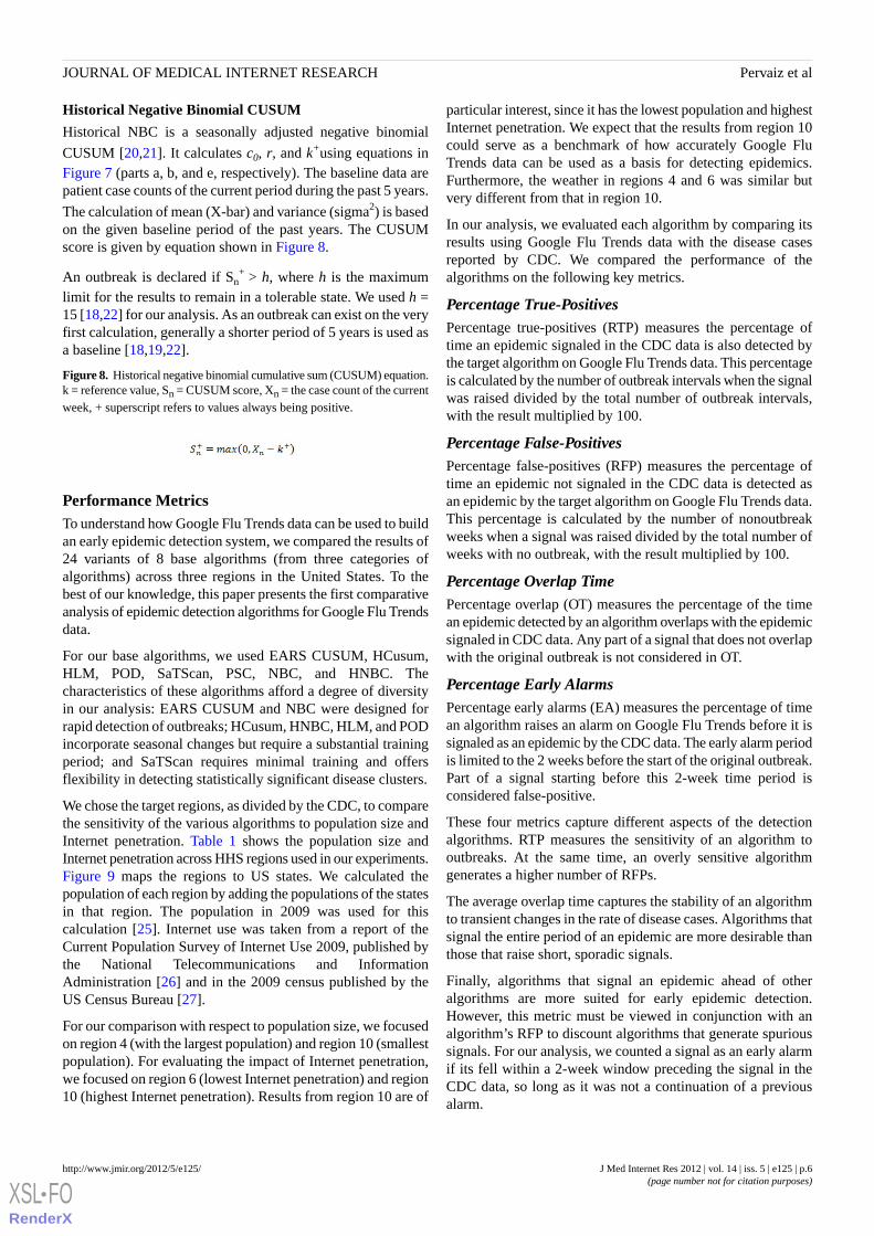
The calculation of mean (X-bar) and variance (sigma2) is basedon the given baseline period of the past years. The CUSUMscore is given by equation shown in Figure 8.

An outbreak is declared if Sn+ > h, where h is the maximum

limit for the results to remain in a tolerable state. We used h =15 [18,22] for our analysis. As an outbreak can exist on the veryfirst calculation, generally a shorter period of 5 years is used asa baseline [18,19,22].

Figure 8. Historical negative binomial cumulative sum (CUSUM) equation.k = reference value, Sn = CUSUM score, Xn = the case count of the currentweek, + superscript refers to values always being positive.

Performance MetricsTo understand how Google Flu Trends data can be used to buildan early epidemic detection system, we compared the results of24 variants of 8 base algorithms (from three categories ofalgorithms) across three regions in the United States. To thebest of our knowledge, this paper presents the first comparativeanalysis of epidemic detection algorithms for Google Flu Trendsdata.

For our base algorithms, we used EARS CUSUM, HCusum,HLM, POD, SaTScan, PSC, NBC, and HNBC. Thecharacteristics of these algorithms afford a degree of diversityin our analysis: EARS CUSUM and NBC were designed forrapid detection of outbreaks; HCusum, HNBC, HLM, and PODincorporate seasonal changes but require a substantial trainingperiod; and SaTScan requires minimal training and offersflexibility in detecting statistically significant disease clusters.

We chose the target regions, as divided by the CDC, to comparethe sensitivity of the various algorithms to population size andInternet penetration. Table 1 shows the population size andInternet penetration across HHS regions used in our experiments.Figure 9 maps the regions to US states. We calculated thepopulation of each region by adding the populations of the statesin that region. The population in 2009 was used for thiscalculation [25]. Internet use was taken from a report of theCurrent Population Survey of Internet Use 2009, published bythe National Telecommunications and InformationAdministration [26] and in the 2009 census published by theUS Census Bureau [27].

For our comparison with respect to population size, we focusedon region 4 (with the largest population) and region 10 (smallestpopulation). For evaluating the impact of Internet penetration,we focused on region 6 (lowest Internet penetration) and region10 (highest Internet penetration). Results from region 10 are of

particular interest, since it has the lowest population and highestInternet penetration. We expect that the results from region 10could serve as a benchmark of how accurately Google FluTrends data can be used as a basis for detecting epidemics.Furthermore, the weather in regions 4 and 6 was similar butvery different from that in region 10.

In our analysis, we evaluated each algorithm by comparing itsresults using Google Flu Trends data with the disease casesreported by CDC. We compared the performance of thealgorithms on the following key metrics.

Percentage True-PositivesPercentage true-positives (RTP) measures the percentage oftime an epidemic signaled in the CDC data is also detected bythe target algorithm on Google Flu Trends data. This percentageis calculated by the number of outbreak intervals when the signalwas raised divided by the total number of outbreak intervals,with the result multiplied by 100.

Percentage False-PositivesPercentage false-positives (RFP) measures the percentage oftime an epidemic not signaled in the CDC data is detected asan epidemic by the target algorithm on Google Flu Trends data.This percentage is calculated by the number of nonoutbreakweeks when a signal was raised divided by the total number ofweeks with no outbreak, with the result multiplied by 100.

Percentage Overlap TimePercentage overlap (OT) measures the percentage of the timean epidemic detected by an algorithm overlaps with the epidemicsignaled in CDC data. Any part of a signal that does not overlapwith the original outbreak is not considered in OT.

Percentage Early AlarmsPercentage early alarms (EA) measures the percentage of timean algorithm raises an alarm on Google Flu Trends before it issignaled as an epidemic by the CDC data. The early alarm periodis limited to the 2 weeks before the start of the original outbreak.Part of a signal starting before this 2-week time period isconsidered false-positive.

These four metrics capture different aspects of the detectionalgorithms. RTP measures the sensitivity of an algorithm tooutbreaks. At the same time, an overly sensitive algorithmgenerates a higher number of RFPs.

The average overlap time captures the stability of an algorithmto transient changes in the rate of disease cases. Algorithms thatsignal the entire period of an epidemic are more desirable thanthose that raise short, sporadic signals.

Finally, algorithms that signal an epidemic ahead of otheralgorithms are more suited for early epidemic detection.However, this metric must be viewed in conjunction with analgorithm’s RFP to discount algorithms that generate spurioussignals. For our analysis, we counted a signal as an early alarmif its fell within a 2-week window preceding the signal in theCDC data, so long as it was not a continuation of a previousalarm.

J Med Internet Res 2012 | vol. 14 | iss. 5 | e125 | p.6http://www.jmir.org/2012/5/e125/(page number not for citation purposes)

Pervaiz et alJOURNAL OF MEDICAL INTERNET RESEARCH

XSL•FORenderX

Table 1. Population and percentage Internet use by US Department of Health and Human Services (HHS) region.

States% Internet

use

Population

(2009 census)

HHS

region

CT, ME, MA, NH, RI, VT74.0714,412,6841

NJ, NY70.2028,224,1142

DE, DC, MD, PA, VA, WV69.3029,479,3613

AL, FL, GA, KY, MS, NC, SC, TN63.2560,088,1784

IL, IN, MI, MN, OH, WI71.4251,745,4105

AR, LA, NM, OK, TX61.5637,860,5496

IA, KS, MO, NE71.6831,840,1787

CO, MT, ND, SD, UT, WY72.1320,802,7858

AZ, CA, HI, NV67.9546,453,0109

AK, ID, OR, WA76.936,691,32510

Figure 9. US Department of Health and Human Services regions.

Results

Figure 10, Figure 11, and Figure 12 compare all of thealgorithms in our study on a 9-year timescale between 2003 and2011. Details for these figures are presented in MultimediaAppendix 1, Multimedia Appendix 2, and Multimedia Appendix3, which compare the algorithms according to our fourcomparison metrics: RTP, RFP, OT, and EA across our threetarget regions [12,13,22].

In each Multimedia Appendix there is a sorted column (overallposition of algorithm). In this column the algorithms are sortedbased on their median across the four performance metrics. Wechose the median to cater for extreme values in the performancemetrics.

Although we have divided the algorithms into three categories,namely Poisson, negative binomial, and normal distributionalgorithms, another subcategory called historical algorithmssurfaced during our analysis. This is a subset of both negativebinomial and normal distribution categories, as it has algorithms

J Med Internet Res 2012 | vol. 14 | iss. 5 | e125 | p.7http://www.jmir.org/2012/5/e125/(page number not for citation purposes)

Pervaiz et alJOURNAL OF MEDICAL INTERNET RESEARCH

XSL•FORenderX

in both. HNBC from the negative binomial and HLM, andHCusum from the normal distribution showed a similar patternof results across the four performance metrics. Therefore, forthe remainder of the discussion, we will add the classificationof historical algorithm and analyze its results independently.

In Table 2, for the first performance metric, RTP, all thecategories had high average values (96.4%, 99.0%, and 98.8%for normal, NBC, and Poisson distribution algorithms,respectively), with the only exception being the historicalalgorithms (64%). Moreover, among the algorithms showing ahigh RTP percentage, there were no significant differencesbetween the values.

In the second performance metric, RFP, values go the other wayround, with the historical algorithms showing remarkablyoptimal values (average 3.3%, where lower is better), whereasnormal, NBC, and Poisson distribution algorithms showpercentages of 11.4%, 28.3%, and 17.5%, respectively. Clearlythe historical algorithms and normal distribution algorithms ledin this metric.

In the third metric, OT, negative binomial distributionalgorithms led, with an OT of 71.3%, followed by Poissondistribution (60.3%), historical algorithms (30.8%), and normaldistribution algorithms (16.4%). In this metric, NBC and Poissondistribution led by a major difference, ahead of historical andnormal distribution algorithms.

In the fourth and last metric, EA, negative binomial, on average,led with an EA value of 75.8%, followed by Poisson distribution(55.1%), normal distribution (36.8%) and historical algorithms(22.3%).

For some performance metrics, certain categories did notperform consistently, and values of these categories varied overa large range. In normal distribution algorithms, the values ofEA varied from 0% to 75%. In Poisson distribution algorithms,EA varied from 13% to 75%. Therefore, in these cases theaverage value of that particular metric could not be considered

representative, and we needed to examine the algorithms (orvariations of algorithms) for suitability.

When we looked at EA values in normal distribution algorithms,the C3 variations of EARS showed a high EA value for onlyone region. Otherwise, the next best values were barely in theoptimal range. Moreover, the OT of C3 at best was 34, whichis very low and made this algorithm not suitable.

In case of the EA values in Poisson distributions, the SaTScanalgorithm pulled the average of Poisson distribution algorithmsdown in EA. Therefore, if we considered the average EA valueof Poisson distribution algorithms without SaTScan, it actuallyrose from 55.1 to 66.7.

Overall, negative binomial and Poisson distribution algorithmsperformed much better than normal distribution algorithms.This is mainly because of the data distribution that thesealgorithms expect. The VMR of seasonal influenza-like illnessdata was greater than 1, most of the time (Figure 13). Therefore,the data followed a negative binomial distribution [28].Moreover, the Poisson distribution was an approximation ofthe negative binomial distribution [29,30]. Therefore, the overallpercentages of both Poisson-based and negative binomial-basedalgorithms turned out to be high.

Historical algorithms performed poorly because they considereddata during the same period in past years to declare the outbreak.They did not consider the distribution of data during the currentyear. This made them robust in terms of false-positives, but theperformance across other metrics lagged by a substantialdifference.

Furthermore, to understand the impact of population variationand change in Internet penetration across regions, we pickedthe top two algorithms from the negative binomial distributionand Poisson distribution algorithms and applied them to all theregions (instead of just three). Table 3, Table 4, Table 5, andTable 6 present the results of the algorithms applied.

The result of this analysis showed that in regions of high Internetpenetration the RFP and OT were high.

Table 2. Average percentages of various performance metrics for various categories of algorithms.

HistoricalPoissonNegative

binomial

NormalMetric

64.098.899.096.4RTPa

3.317.528.311.4RFPb

30.860.371.316.4OTc

22.355.175.836.8EAd

a Percentage true-positives.b Percentage false-positives.c Percentage overlap time.d Percentage early alarms.

J Med Internet Res 2012 | vol. 14 | iss. 5 | e125 | p.8http://www.jmir.org/2012/5/e125/(page number not for citation purposes)

Pervaiz et alJOURNAL OF MEDICAL INTERNET RESEARCH

XSL•FORenderX

Table 3. Result of negative binomial cumulative sum (cut-off = 15), for all performance metrics across all Department of Health and Human Services(HHS) regions of the United States.

EAdOTcRFPbRTPaHHS region

87.598451001

77.785401002

87.588401003

8881301004

87.595401005

8876401006

87.595401007

75835087.58

807140909

71824010010

a Percentage true-positives.b Percentage false-positives.c Percentage overlap time.d Percentage early alarms.

Table 4. Result of negative binomial cumulative sum (threshold = 1 * k) for all performance metrics across all Department of Health and HumanServices (HHS) regions of the United States.

EAdOTcRFPbRTPaHHS region

87.587351001

66.774271002

7581201003

7570201004

7586301005

7563201006

7587301007

75714087.58

706430909

71683010010

a Percentage true-positives.b Percentage false-positives.c Percentage overlap time.d Percentage early alarms.

J Med Internet Res 2012 | vol. 14 | iss. 5 | e125 | p.9http://www.jmir.org/2012/5/e125/(page number not for citation purposes)

Pervaiz et alJOURNAL OF MEDICAL INTERNET RESEARCH

XSL•FORenderX

Table 5. Result of Poisson cumulative sum (threshold = 1 * k) for all performance metrics across all Department of Health and Human Services (HHS)regions of the United States.

EAdOTcRFPbRTPaHHS region

87.583351001

66.771271002

7580201003

7570201004

7584301005

7562201006

7584301007

75674087.58

706430909

57683010010

a Percentage true-positives.b Percentage false-positives.c Percentage overlap time.d Percentage early alarms.

Table 6. Result of Poisson outbreak detection for all performance metrics across all Department of Health and Human Services (HHS) regions of theUnited States.

EAdOTcRFPbRTPaHHS region

3377351001

4070201002

5069301003

7558201004

5072401005

7550201006

7572301007

75743087.58

405720909

57682010010

a Percentage true-positives.b Percentage false-positives.c Percentage overlap time.d Percentage early alarms.

J Med Internet Res 2012 | vol. 14 | iss. 5 | e125 | p.10http://www.jmir.org/2012/5/e125/(page number not for citation purposes)

Pervaiz et alJOURNAL OF MEDICAL INTERNET RESEARCH

XSL•FORenderX

Figure 10. US Department of Health and Human Services region 4. The x-axis plots the Google Flu Trends and Centers for Disease Control andPrevention (CDC) data. The horizontal bars indicate where each method detected an epidemic. Cut indicates the cut-off point (more is less sensitive)and b indicates baseline data (training window). The thick horizontal bars at the bottom show the actual outbreak. HCusum = historical cumulative sum,HLM = historical limits method, HNBC = historical negative binomial cumulative sum, ILI = influenza-like illnesses, k = reference value for threshold,NBC = negative binomial cumulative sum, POD = Poisson outbreak detection, PSC = Poisson cumulative sum.

J Med Internet Res 2012 | vol. 14 | iss. 5 | e125 | p.11http://www.jmir.org/2012/5/e125/(page number not for citation purposes)

Pervaiz et alJOURNAL OF MEDICAL INTERNET RESEARCH

XSL•FORenderX

Figure 11. US Department of Health and Human Services region 6. The x-axis plots the Google Flu Trends and Centers for Disease Control andPrevention (CDC) data. The horizontal bars indicate where each method detected an epidemic. Cut indicates cut-off point (more is less sensitive) andb indicates baseline data (training window). The thick horizontal bar at the bottom shows the actual outbreak. HCusum = historical cumulative sum,HLM = historical limits method, HNBC = historical negative binomial cumulative sum, ILI = influenza-like illnesses, k = reference value for threshold,NBC = negative binomial cumulative sum, POD = Poisson outbreak detection, PSC = Poisson cumulative sum.

J Med Internet Res 2012 | vol. 14 | iss. 5 | e125 | p.12http://www.jmir.org/2012/5/e125/(page number not for citation purposes)

Pervaiz et alJOURNAL OF MEDICAL INTERNET RESEARCH

XSL•FORenderX

Figure 12. US Department of Health and Human Services region 10. The x-axis plots the Google Flu Trends and Centers for Disease Control andPrevention (CDC) data. The horizontal bars indicate where each method detected an epidemic. Cut indicates cut-off point (more is less sensitive) andb indicates baseline data (training window). The thick horizontal bar at the bottom shows actual outbreak. HCusum = historical cumulative sum, HLM= historical limits method, HNBC = historical negative binomial cumulative sum, ILI = influenza-like illnesses, k = reference value for threshold, NBC= negative binomial cumulative sum, POD = Poisson outbreak detection, PSC = Poisson cumulative sum.

Figure 13. US Centers for Disease Control and Prevention data with the variance to mean ratio (VMR) line above, along the VMR = 1 mark.

J Med Internet Res 2012 | vol. 14 | iss. 5 | e125 | p.13http://www.jmir.org/2012/5/e125/(page number not for citation purposes)

Pervaiz et alJOURNAL OF MEDICAL INTERNET RESEARCH

XSL•FORenderX

Discussion

In this study, we augmented the capabilities of Google FluTrends by evaluating various algorithms to translate the rawsearch query volume produced by this service into actionablealerts. We focused, in particular, on leveraging the ability ofGoogle Flu Trends to provide a near real-time alternative toconventional disease surveillance networks and to explore thepracticality of building an early epidemic detection system usingthese data. This paper presents the first detailed comparativeanalysis of popular early epidemic detection algorithms onGoogle Flu Trends. We explored the relative merits of thesemethods and considered the effects of changing Internetprevalence and population sizes on the ability of these methodsto predict epidemics. In these evaluations, we drew upon datacollected by the CDC and assessed the ability of each algorithmwithin a consistent experimental framework to predict changesin measured CDC case frequencies from the Internet searchquery volume.

Our analysis showed that adding a layer of computationalintelligence to Google Flu Trends data provides the opportunityfor a reliable early epidemic detection system that can predictdisease outbreaks with high accuracy in advance of the existingsystems used by the CDC. However, we note that realizing thisopportunity requires moving beyond the CUSUM- andHLM-based normal distribution approaches traditionallyemployed by the CDC. In particular, while we did not find asingle best method to apply to Google Flu Trends data, theresults of our study strongly support negative binomial- andPoisson-based algorithms being more useful when dealing withpotentially noisy search query data from regions with varyingInternet penetrations. For such data, we found that normaldistribution algorithms did not perform as well as the negativebinomial and Poisson distribution algorithms.

Furthermore, our analysis showed that the patient data of adisease follows different distributions throughout the year.Therefore, when VMR of data is equal to 1, it is ideallyfollowing a Poisson distribution and could be handled by aPoisson-based algorithm. As the increase in variance raisesVMR above 1, the data become overdispersed. Poisson-basedalgorithms can handle this overdispersion, up to a limit [29].When VMR is very high, an algorithm is needed that considersthe variance as a parameter and raises alarms accordingly. Since

negative binomial distribution-based algorithms consider thevariance [29], such algorithms perform better in similarscenarios. For instance, NBC is accurate in raising an alarm foroverdispersed count data [29]. To get better results, we proposean approach, based on the above discussion, of changing thedistribution expectation of an algorithm along with the rise andfall in VMR. This area should be explored in more depth toproduce algorithms that adapt according to the data’s distributiontype.

Our research is the first attempt of its kind to relate epidemicprediction using Google Flu Trends data to Internet penetrationand the size of the population being assessed. We believe thatunderstanding how these factors affect algorithms to predictepidemics is an integral question for scaling a searchquery-based system to a broad range of geographical regionsand communities. In our investigations, we observed that bothInternet penetration and population size had a definite impacton algorithm performance. SaTScan performs better whenapplied to data from regions with high Internet penetration andsmall population size, while POD and NBC achieves betterresults when Internet penetration is low and population size islarge. CUSUM performs best in regions with a large population.While the availability of search query data and measured (ie,CDC) case records restrict our analyses to the United States,we believe many of these insights may be useful in developingan early epidemic prediction system for other regions, includingcommunities in the developing world.

In conclusion, we present an early investigation of algorithmsto translate data from services such as Google Flu Trends intoa fully automated system for generating alerts when thelikelihood of epidemics is quite high. Our research augmentsthe ability to detect disease outbreaks at early stages, whenmany of the conditions that impose an immense burden globallycan be treated with better outcomes and in a more cost-effectivemanner. In addition, the ability to respond early to imminentconditions allows for more proactive restriction of the size ofany potential outbreak. Together, the findings of our studyprovide a means to convert raw data collected over the Internetinto more fine-grained information that can guide effectivepolicy in countering the spread of diseases.

Based on our work, we have developed FluBreaks(dritte.org/flubreaks), an early warning system for flu epidemicsusing Google Flu Trends.

 

AcknowledgmentsWe acknowledge Dr Zeeshan Syed of the University of Michigan for his valuable feedback and intellectual contribution. Wethank Dr Farkanda Kokab, Professor of Epidemiology, Institute of Public Health, Pakistan, and Dr Ijaz Shah, Professor and Headof Department of Community Medicine, Quaid-e-Azam Medical College, Pakistan, for marking our outbreaks and providing uswith valuable feedback. We also thank Dr Lakshminarayanan Subramanian of New York University for reviewing our paper.

Conflicts of InterestNone declared.

Multimedia Appendix 1Ranking of algorithms in different parameters of evaluation for HSS Region 4 (Highest Population).

J Med Internet Res 2012 | vol. 14 | iss. 5 | e125 | p.14http://www.jmir.org/2012/5/e125/(page number not for citation purposes)

Pervaiz et alJOURNAL OF MEDICAL INTERNET RESEARCH

XSL•FORenderX

[PDF File (Adobe PDF File), 48KB - jmir_v14i5e125_app1.pdf ]

Multimedia Appendix 2Ranking of algorithms in different parameters of evaluation for HSS Region 6 (Lowest Percent Internet Use).

[PDF File (Adobe PDF File), 48KB - jmir_v14i5e125_app2.pdf ]

Multimedia Appendix 3Ranking of algorithms in different parameters of evaluation for HSS Region 10 (Lowest Population and Highest Percent InternetUse).

[PDF File (Adobe PDF File), 48KB - jmir_v14i5e125_app3.pdf ]

References1. Eysenbach G. Infodemiology and infoveillance: framework for an emerging set of public health informatics methods to

analyze search, communication and publication behavior on the Internet. J Med Internet Res 2009;11(1):e11 [FREE Fulltext] [doi: 10.2196/jmir.1157] [Medline: 19329408]

2. Eysenbach G. Infodemiology: tracking flu-related searches on the web for syndromic surveillance. AMIA Annu Symp Proc2006:244-248. [Medline: 17238340]

3. Bennett GG, Glasgow RE. The delivery of public health interventions via the Internet: actualizing their potential. AnnuRev Public Health 2009;30:273-292. [doi: 10.1146/annurev.publhealth.031308.100235] [Medline: 19296777]

4. Castillo-Salgado C. Trends and directions of global public health surveillance. Epidemiol Rev 2010 Apr;32(1):93-109.[doi: 10.1093/epirev/mxq008] [Medline: 20534776]

5. Ginsberg J, Mohebbi MH, Patel RS, Brammer L, Smolinski MS, Brilliant L. Detecting influenza epidemics using searchengine query data. Nature 2009 Feb 19;457(7232):1012-1014. [doi: 10.1038/nature07634] [Medline: 19020500]

6. Wilson K, Brownstein JS. Early detection of disease outbreaks using the Internet. CMAJ 2009 Apr 14;180(8):829-831.[doi: 10.1503/cmaj.090215] [Medline: 19364791]

7. Seifter A, Schwarzwalder A, Geis K, Aucott J. The utility of "Google Trends" for epidemiological research: Lyme diseaseas an example. Geospat Health 2010 May;4(2):135-137 [FREE Full text] [Medline: 20503183]

8. Breyer BN, Sen S, Aaronson DS, Stoller ML, Erickson BA, Eisenberg ML. Use of Google Insights for Search to trackseasonal and geographic kidney stone incidence in the United States. Urology 2011 Aug;78(2):267-271. [doi:10.1016/j.urology.2011.01.010] [Medline: 21459414]

9. Google. 2012 Mar 6. Flu Trends: United States 2011-2012 URL: http://www.google.org/flutrends/us/ [accessed 2012-03-08][WebCite Cache ID 660ZkIfcu]

10. Hutwagner L, Thompson W, Seeman GM, Treadwell T. The bioterrorism preparedness and response Early AberrationReporting System (EARS). J Urban Health 2003 Jun;80(2 Suppl 1):i89-i96. [Medline: 12791783]

11. Fricker RD, Hegler BL, Dunfee DA. Comparing syndromic surveillance detection methods: EARS' versus a CUSUM-basedmethodology. Stat Med 2008 Jul 30;27(17):3407-3429. [doi: 10.1002/sim.3197] [Medline: 18240128]

12. Hutwagner LC, Thompson WW, Seeman GM, Treadwell T. A simulation model for assessing aberration detection methodsused in public health surveillance for systems with limited baselines. Stat Med 2005 Feb 28;24(4):543-550. [doi:10.1002/sim.2034] [Medline: 15678442]

13. Stroup DF, Williamson GD, Herndon JL, Karon JM. Detection of aberrations in the occurrence of notifiable diseasessurveillance data. Stat Med 1989 Mar;8(3):323-9; discussion 331. [Medline: 2540519]

14. Hutwagner LC, Maloney EK, Bean NH, Slutsker L, Martin SM. Using laboratory-based surveillance data for prevention:an algorithm for detecting Salmonella outbreaks. Emerg Infect Dis 1997;3(3):395-400. [doi: 10.3201/eid0303.970322][Medline: 9284390]

15. Hutwagner L, Browne T, Seeman GM, Fleischauer AT. Comparing aberration detection methods with simulated data.Emerg Infect Dis 2005 Feb;11(2):314-316 [FREE Full text] [doi: 10.3201/eid1102.040587] [Medline: 15752454]

16. Gatton ML, Kelly-Hope LA, Kay BH, Ryan PA. Spatial-temporal analysis of Ross River virus disease patterns in Queensland,Australia. Am J Trop Med Hyg 2004 Nov;71(5):629-635 [FREE Full text] [Medline: 15569796]

17. Kulldorff M, Information Management Services Inc. satscan.org. 2005. SaTScan: Software for the Spatial, Temporal, andSpace-Time Scan Statistics URL: http://www.satscan.org/ [accessed 2012-03-08] [WebCite Cache ID 660ZfnlJK]

18. Unkel S, Farrington CP, Garthwaite PH, Robertson C, Andrews N. Statistical methods for the prospective detection ofinfectious disease outbreaks: a review. J R Stat Soc 2012;175(1):49-82. [doi: 10.1111/j.1467-985X.2011.00714.x]

19. Lucas JM. Counted data CUSUM's. Technometrics 1985;27(2):129-144 [FREE Full text] [WebCite Cache]20. Hawkins DM, Olwell DH. Cumulative Sum Charts and Charting for Quality Improvement. New York, NY: Springer; 1998.

J Med Internet Res 2012 | vol. 14 | iss. 5 | e125 | p.15http://www.jmir.org/2012/5/e125/(page number not for citation purposes)

Pervaiz et alJOURNAL OF MEDICAL INTERNET RESEARCH

XSL•FORenderX

21. Watkins RE, Eagleson S, Veenendaal B, Wright G, Plant AJ. Applying cusum-based methods for the detection of outbreaksof Ross River virus disease in Western Australia. BMC Med Inform Decis Mak 2008;8:37 [FREE Full text] [doi:10.1186/1472-6947-8-37] [Medline: 18700044]

22. Pelecanos AM, Ryan PA, Gatton ML. Outbreak detection algorithms for seasonal disease data: a case study using RossRiver virus disease. BMC Med Inform Decis Mak 2010;10:74 [FREE Full text] [doi: 10.1186/1472-6947-10-74] [Medline:21106104]

23. Centers for Disease Control and Prevention. 2012 Mar 2. Seasonal Influenza (Flu): 2011-2012 Influenza Season Week 8Ending February 25, 2012 URL: http://www.cdc.gov/flu/weekly/ [accessed 2012-03-08] [WebCite Cache ID 660YMRZYi]

24. Centers for Disease Control and Prevention. 2011 Oct 7. Seasonal Flu (Influenza): Overview of Influenza Surveillance inthe United States URL: http://www.cdc.gov/flu/weekly/overview.htm [accessed 2012-05-15] [WebCite Cache ID 67gSoQJVS]

25. Fact Monster. Pearson Education. 2012. U.S. Population by State, 1790 to 2010 URL: http://www.factmonster.com/ipka/A0004986.html [accessed 2012-03-08] [WebCite Cache ID 660XsTmos]

26. US Department of Commerce, National Telecommunications & Information Administration. 2009. Current PopulationSurvey (CPS) Internet Use 2009 URL: http://www.ntia.doc.gov/data/CPS2009_Tables.html [accessed 2012-03-08] [WebCiteCache ID 660Y9BiVr]

27. US Department of Commerce, National Telecommunications and Information Administration. US Census Bureau, StatisticalAbstract of the United States. 2011. Household Internet Usage by Type of Internet Connection and State: 2009 URL: http://www.census.gov/compendia/statab/2011/tables/11s1155.pdf [accessed 2012-03-08] [WebCite Cache ID 660YHNY66]

28. Cox DR, Lewis P. The Statistical Analysis of Series of Events. London: Chapman and Hall; 1966.29. McCullagh P, Nelder JA. Generalized Linear Models. 2nd edition. London: Chapman and Hall; 1989.30. Cameron AC, Trivedi. Regression Analysis of Count Data. Cambridge, UK: Cambridge University Press; 1998.

AbbreviationsCDC: Centers for Disease Control and PreventionCUSUM: cumulative sumEA: percentage early alarmsEARS: Early Aberration Reporting SystemHCusum: historical cumulative sumHLM: historical limits methodILINet: Outpatient Influenza-like Illness Surveillance NetworkNBC: negative binomial cumulative sumOT: percentage overlapPOD: Poisson outbreak detectionPSC: Poisson cumulative sumRFP: percentages false-positivesRTP: percentage true-positivesVMR: variance to mean ratio

Edited by G Eysenbach; submitted 08.03.12; peer-reviewed by M Gatton; comments to author 29.03.12; revised version received18.05.12; accepted 10.07.12; published 04.10.12

Please cite as:Pervaiz F, Pervaiz M, Abdur Rehman N, Saif UFluBreaks: Early Epidemic Detection from Google Flu TrendsJ Med Internet Res 2012;14(5):e125URL: http://www.jmir.org/2012/5/e125/ doi:10.2196/jmir.2102PMID:23037553

©Fahad Pervaiz, Mansoor Pervaiz, Nabeel Abdur Rehman, Umar Saif. Originally published in the Journal of Medical InternetResearch (http://www.jmir.org), 04.10.2012. This is an open-access article distributed under the terms of the Creative CommonsAttribution License (http://creativecommons.org/licenses/by/2.0/), which permits unrestricted use, distribution, and reproductionin any medium, provided the original work, first published in the Journal of Medical Internet Research, is properly cited. Thecomplete bibliographic information, a link to the original publication on http://www.jmir.org/, as well as this copyright and licenseinformation must be included.

J Med Internet Res 2012 | vol. 14 | iss. 5 | e125 | p.16http://www.jmir.org/2012/5/e125/(page number not for citation purposes)

Pervaiz et alJOURNAL OF MEDICAL INTERNET RESEARCH

XSL•FORenderX