ARTICLE IN PRESS

0360-1323/$ - se

doi:10.1016/j.bu

�Correspondof Engineering,

NSW 2308, Au

E-mail addr

Building and Environment 43 (2008) 37–43

www.elsevier.com/locate/buildenv

A new stable finite volume method for predicting thermalperformance of a whole building

C. Luo�, B. Moghtaderi, H. Sugo, A. Page

School of Engineering, Faculty of Engineering & Built Environment, The University of Newcastle, University Drive, Callaghan NSW 2308, Australia

Received 2 August 2006; received in revised form 7 November 2006; accepted 27 November 2006

Abstract

Discretised governing equations involving only temperatures and heat fluxes at both surfaces of a solid wall layer were obtained by

combining a new stable finite volume scheme for the two inner nodes of the wall layer with the surface diffusion equations (discretised by

third order equations). The finite volume scheme for the inner nodes of the layer is proved to be stable with its truncation error being

OðDx4;Dx2Dt2Þ. A special analytical solution for a solid wall was used to evaluate different schemes for the inner nodes, showing that the

new proposed scheme performs better than all other schemes for time steps of 3600 and 600 s. Finally, this scheme was used to simulate a

whole house and the predicted zonal air temperature, and surface temperatures agreed well with measured values.

r 2007 Elsevier Ltd. All rights reserved.

Keywords: Finite volume method; Finite difference method; Fourier stability analysis; Thermal zone model; Fourier diffusion equation

1. Introduction

A thermal zonal model assumes that all independentvariables are distributed uniformly across the building wallsand within the zones (such as room air or the air cavity in acavity wall) and combines the heat balance equations forsolid walls with the energy balance equations for the zonalair. To simplify the heat balance equations for solid walls,the response factor method and the conduction transferfunction (CTF) method have been adopted in a number ofcommercial and scientific software programs, such asTRNSYS, Energy Plus (CTF) and AccuRate (ResponseFactor). To avoid solving the governing equations for theinner nodes of a wall layer, SUNCODE used an explicitdifference scheme to solve the wall conduction equations.However, it is well known that the explicit difference schemehas a stability problem. Because of potential stabilityproblems and the storage requirements for the inner nodes,SUNCODE is only suitable for residential or small

e front matter r 2007 Elsevier Ltd. All rights reserved.

ildenv.2006.11.037

ing author. Department of Chemical Engineering, School

The University of Newcastle, University Drive, Callaghan

stralia. Tel.: +61 2 4921 6951; fax: +61 2 4921 8692.

ess: Caimao.Luo@newcastle.edu.au (C. Luo).

commercial buildings. The inner node equations preventresearchers using the finite difference method for modellingthe thermal performance of buildings. Therefore, to utilisethe finite difference method in the thermal performancemodelling of buildings, it is necessary to construct a schemewhich does not involve the inner nodes.Tsilingiris [1,2] used the Laasonen scheme to develop a

finite difference method to study the thermal behaviour ofwalls. He utilized the effective thermal capacitance andthermal conductivity to simplify the parallel layers of thecomposite material with Dx ¼ 1 cm and Dt ¼ 60–300 s (or1–5min). It is not made clear by the author whether or notthe method could be applied to a whole building.The study reported in this paper focuses on a finite

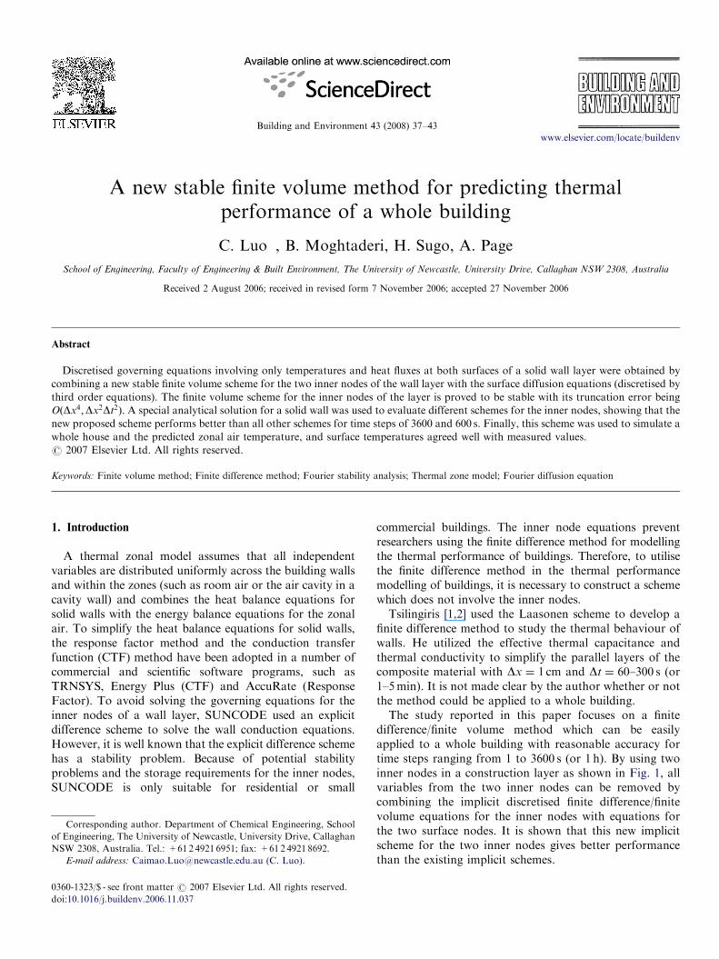
difference/finite volume method which can be easilyapplied to a whole building with reasonable accuracy fortime steps ranging from 1 to 3600 s (or 1 h). By using twoinner nodes in a construction layer as shown in Fig. 1, allvariables from the two inner nodes can be removed bycombining the implicit discretised finite difference/finitevolume equations for the inner nodes with equations forthe two surface nodes. It is shown that this new implicitscheme for the two inner nodes gives better performancethan the existing implicit schemes.

ARTICLE IN PRESS

Ts0 T2 Ts1

q"s0 "s1q

T1

Fig. 1. Illustration of variables for a single layer in a brickwork wall.

C. Luo et al. / Building and Environment 43 (2008) 37–4338

2. Discretised governing equations for inner nodes

The key differences for existing building thermalperformance software come from the treatment of solidwalls. The Fourier diffusion equation for a solid wall is

rCpqT

qt¼ k

q2Tqx2

(1)

in which r denotes density, Cp is the specific capacity,k is the thermal conductivity of the layer, T is thetemperature across the layer, t is the time and x is thedistance across the layer. A new finite volume schemeand a hybrid finite volume–finite difference scheme fordiscretizing the partial differential equation are presentedbelow.

2.1. Finite volume discretised schemes for the solid Fourier

heat transfer equation

Because of the large amount of cpu time consumed insolving the resulting system of equations, for any singlelayer (in this case a masonry wall), only four nodes areconsidered as illustrated in Fig. 1. For the inner nodes, T1

and T2, the spatially discretised equations are obtained byintegrating the domains ½xs0;x2� and ½x1;xs1� with Simp-son’s 1

3integration law, respectively, as follows:

1

3DxrbCpb

qT s0

qtþ 4

qT1

qtþ

qT2

qt

� �

¼ �kqT

qx

����s0

þ kqT

qx

����2

¼2k

DxðT s0 � 2T1 þ T2Þ, ð2Þ

1

3DxrbCpb

qT1

qtþ 4

qT2

qtþ

qT s1

qt

� �

¼ �kqT

qx

����1

þ kqT

qx

����s1

¼2k

DxðT1 � 2T2 þ T s1Þ. ð3Þ

Integrating Eqs. (2) and (3) over the time domain ½t� Dt; t�,it reads

L2t rCpb

27kDt½ðT s0 þ 4T1 þ T2Þ

n� ðT s0 þ 4T1 þ T2Þ

n�1�

¼ ½ðT s0 � 2T1 þ T2Þnþ ðT s0 � 2T1 þ T2Þ

n�1�, ð4Þ

L2t rCpb

27kDt½ðT1 þ 4T2 þ T s1Þ

n� ðT1 þ 4T2 þ T s1Þ

n�1�

¼ ½ðT1 � 2T2 þ T s1Þnþ ðT1 � 2T2 þ T s1Þ

n�1�. ð5Þ

In which n denotes the instant time t; ðn� 1Þ denotes timeðt� DtÞ, rCp denotes the product of the density r and itsspecific capacity Cp, Lt is the thickness of the material andk is the thermal conductivity of the layer. The truncationerror (T.E.) for this finite volume scheme is

T.E. ¼rCpb

k

1

6

q4Tqx4

����n

Dx4 �1

12

q4Tqx2qt2

����n

Dx4Dt

"

þ1

36

q5T

qx4qt

����n

Dx6 �1

72

q6Tqx4qt2

����n

Dx6Dt

#

�1

6

q4T

qx2qt2

����n

Dx2Dt2 þ1

48

q6Tqx4qt2

����n

Dx4Dt2. ð6Þ

This scheme is termed as Scheme I in this paper. It shouldbe noted that a discretised scheme can also be obtained byapplying Simpson 1

3integration over the time domain

½t� 2Dt; t�. However, in this case this scheme was proven tobe unstable.

2.2. A hybrid finite volume—finite difference scheme

Starting from Eqs. (2) and (3) obtained by applyingfinite volume method, a finite difference scheme of secondorder of accuracy for discretizing the q=qt terms of theleft-hand sides of Eqs. (2) and (3), employing qj=qt ¼

ð3jn � 4jn�1 þ jn�2Þ=2Dt, can be obtained as follows:

L2t rCpb

108kDt½3ðT s0 þ 4T1 þ T2Þ

n� 4ðT s0 þ 4T1 þ T2Þ

n�1

þ ðT s0 þ 4T1 þ T2Þn�2� ¼ ðT s0 � 2T1 þ T2Þ

n, ð7Þ

L2t rCpb

108kDt½3ðT1 þ 4T2 þ T s1Þ

n� 4ðT1 þ 4T2 þ T s1Þ

n�1

þ ðT1 þ 4T2 þ T s1Þn�2� ¼ ðT1 � 2T2 þ T s1Þ

n. ð8Þ

This scheme is termed as Scheme II in the paper.

2.3. A fifth order accuracy of hybrid finite volume—finite

difference scheme

Starting from Eqs. (2) and (3) obtained by applying thefinite volume method, a finite difference scheme of secondorder of accuracy for discretizing the q=qt terms of the left-hand sides of Eqs. (2) and (3), employing qj=qt ¼ ð50jn�

96jn�1 þ 72jn�2 � 32jn�3 þ 6jn�4Þ=24Dt, can be obtained

ARTICLE IN PRESSC. Luo et al. / Building and Environment 43 (2008) 37–43 39

as follows:

L2t rCpb

1296kDt½50ðT s0 þ 4T1 þ T2Þ

n� 96ðT s0 þ 4T1 þ T2Þ

n�1

þ 72ðT s0 þ 4T1 þ T2Þn�2� 32ðT s0 þ 4T1 þ T2Þ

n�3

þ 6ðT s0 þ 4T1 þ T2Þn�4� ¼ ðT s0 � 2T1 þ T2Þ

n, ð9Þ

L2t rCpb

1296kDt½50ðT1 þ 4T2 þ T s1Þ

n� 96ðT1 þ 4T2 þ T s1Þ

n�1

þ 72ðT1 þ 4T2 þ T s1Þn�2� 32ðT1 þ 4T2 þ T s1Þ

n�3

þ 6ðT1 þ 4T2 þ T s1Þn�4� ¼ ðT1 � 2T2 þ T s1Þ

n. ð10Þ

This scheme is termed as Scheme III in the paper.

3. Fourier stability analyses for the new inner nodes schemes

Assuming Tni ¼ T0rnejbxx for a time t and location of x,

substituting this equation into Eq. (4) for Scheme I,through some algebra operations, we can obtain

L2trCpb

27kDtðr� 1ÞðcosðbxDxÞ þ 2Þ

¼ �ðrþ 1Þð1� cosðbxDxÞÞ. ð11Þ

Recombining (11), and defining b ¼ L2trCpb

=27kDt, itbecomes

r ¼bðcosðbxDxÞ þ 2Þ � ð1� cosðbxDxÞÞ

bðcosðbxDxÞ þ 2Þ þ ð1� cosðbxDxÞÞ. (12)

Because ð1�cosðbxDxÞÞ is non-negative, and bðcosðbxDxÞþ2Þis positive, the denominator in Eq. (12) is larger than or equalto the numerator of Eq. (12), leading to the conclusion thatScheme I is unconditionally stable since �1prp1.

For Scheme II, the amplitude factor equation is

r2

3r2 � 4rþ 1¼ �

L2trCpb

108kDt

ð2þ cosðbxDxÞÞ

ð1� cosðbxDxÞÞ. (13)

It can be shown that jrjp1 (refer to Appendix A),indicating that Scheme II is also unconditionally stable.

Similarly for Scheme III, the amplitude factor equationis

r3 þ 3r2 þ 3rþ 1

ðr3 � 1Þ¼ �

3L2trCpb

216kDt

ð2þ cosðbxDxÞÞ

ð1� cosðbxDxÞÞ. (14)

It is difficult to prove in general that �1prp1, however,for all cases studied, Scheme III was also unconditionallystable.

4. Resulting discretised governing equations for the surface

nodes

The governing equations for surface nodes T s0 and T s1 are

q00s0 � �kqT

qx

����s0

� �¼ 0 or q00s0 þ k

qT

qx

����s0

¼ 0, (15)

�q00s1 þ �kqT

qx

����s1

� �¼ 0 or q00s1 þ k

qT

qx

����s1

¼ 0. (16)

Considering that

qT

qx

����s0

¼1

3Dxð�5:5T s0 þ 9T1 � 4:5T2 þ T s1Þ þOðDx3Þ

(17)

and

qT

qx

����cs1

¼1

3Dxð5:5Tcs1 � 9T2 þ 4:5T1 � T s0Þ þOðDx3Þ.

(18)

Rearranging Eqs. (15)–(18), we can obtain

T1 ¼ �3Dxð2q00s0 � q00s1Þ

13:5kþ

10T s0

13:5þ

3:5T s1

13:5, (19)

T2 ¼ �3Dxðq00s0 � 2q00s1Þ

13:5kþ

3:5T s0

13:5þ

10T s1

13:5. (20)

Substituting Eqs. (19) and (20) back in Eqs. (4) and (5), theresulting discretised equations for Scheme I are

1

162kL2trbCpb

57T s0 þ 24T s1 �9Lt

kq00s0 þ

6Lt

kq00s1

� �n"

� 57T s0 þ 24T s1 �9Lt

kq00s0 þ

6Lt

kq00s1

� �n�1#

¼Dt

2�T s0 þ T s1 þ

Lt

kq00s0

� �n"

þ �T s0 þ T s1 þLt

kq00s0

� �n�1#, ð21Þ

1

162kL2trbCpb

24T s0 þ 57T s1 �6Lt

kq00s0 þ

9Lt

kq00s1

� �n"

� 24T s0 þ 57T s1 �6Lt

kq00s0 þ

9Lt

kq00s1

� �n�1#

¼Dt

2T s0 � T s1 �

Lt

kq00s1

� �n"

þ T s0 � T s1 �Lt

kq00s1

� �n�1#. ð22Þ

Thus, in Eqs. (21) and (22), the variables of the inner nodesare removed.Similarly, the resulting discretised equations for Scheme

II are

3 57T s0 þ 24T s1 �9Lt

kq00s0 þ

6Lt

kq00s1

� �n

� 4 57T s0 þ 24T s1 �9Lt

kq00s0 þ

6Lt

kq00s1

� �n�1

ARTICLE IN PRESS

0.0E+00

1.0E-01

2.0E-01

3.0E-01

4.0E-01

5.0E-01

6.0E-01

7.0E-01

8.0E-01

9.0E-01

0 4 8 12 16 20 24

Time (Hour)

T/T

i (-

)

Finite Volume Scheme

Analytic Solution

Crank-Nicolson Scheme

Bhattacharya Scheme

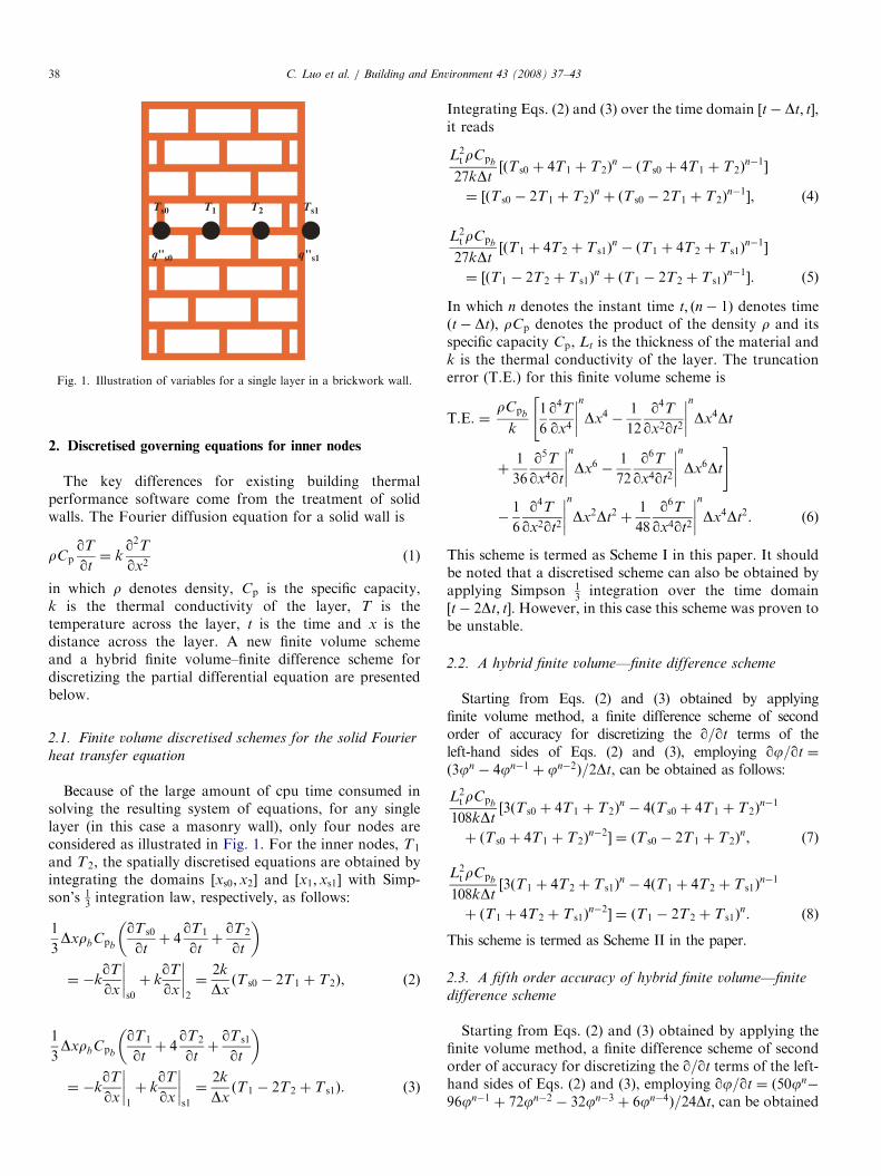
Fig. 2. Evolvement of temperature at the surface of 0.5m thick brickwork

at ðT i ¼Þ10�C exposed to 0 �C atmosphere with one surface kept at

adiabatic condition using different schemes: Dx ¼ 0:5=3m and

Dt ¼ 3600 s.

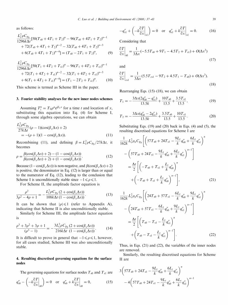
-1.0E+01

-8.0E+00

-6.0E+00

-4.0E+00

-2.0E+00

0.0E+00

2.0E+00

4.0E+00

6.0E+00

0 4 8 12 16 20 24

Time (Hour)

Rela

tive E

rror

(%)

Finite Volume Scheme

Crank-Nicolson Scheme

Bhattacharya Scheme

Fig. 3. Relative error of temperature evolvement at the surface of 0.5m

thick brickwork at 10 �C exposed to 0 �C atmosphere with one surface

kept at adiabatic condition using different schemes: Dx ¼ 0:5=3m and

Dt ¼ 3600 s.

C. Luo et al. / Building and Environment 43 (2008) 37–4340

þ 57T s0 þ 24T s1 �9Lt

kq00s0 þ

6Lt

kq00s1

� �n�2

¼324kDt

L2trbCpb

�T s0 þ T s1 þLt

kq00s0

� �n

, ð23Þ

3 24T s0 þ 57T s1 �6Lt

kq00s0 þ

9Lt

kq00s1

� �n

� 4 24T s0 þ 57T s1 �6Lt

kq00s0 þ

9Lt

kq00s1

� �n�1

þ 24T s0 þ 57T s1 �6Lt

kq00s0 þ

9Lt

kq00s1

� �n�2

¼324kDt

L2trbCpb

T s0 � T s1 �Lt

kq00s1

� �n

. ð24Þ

5. Comparison of the schemes against analytical solutions

and full scale measurements

The Crank–Nicolson Scheme and the Bhattacharyascheme [3] were chosen also to discretize the internalnodes. It is not difficult to obtain similar ‘‘resultingdiscretised equations’’ which only involve temperaturesand heat fluxes at both surfaces for a construction layerand hence these are not presented in the current paper. Allof the derived schemes are evaluated against two analyticalsolutions for a construction layer and one set of actual fullscale measurements from a housing test module.

Case I: A constant temperature construction layer with

one surface kept at an adiabatic condition exposed to the

atmosphere. Assuming the initial temperature of theconstruction layer is set as T i, and the atmospheretemperature is T0 ð¼ 0 �CÞ, and the convective heattransfer coefficient between the layer surface and theatmosphere is hi (W/Km2). The initial condition andboundary conditions for this case can be summarized as thefollowing:

Initial condition

Tðx; t ¼ 0Þ ¼ T i. (25)

Boundary condition at the adiabatic surface

�kqT

qx

����x¼�L

¼ 0. (26)

Boundary condition at x ¼ L

�kqT

qx

����x¼L

¼ hiðT � T0Þ ¼ hiT . (27)

And according to [4], the analytical solution for this case is

Tðx; tÞ ¼ T i

X1n¼1

2B cosðunx=LÞ

ðBþ B2 þ u2nÞ cos un

e�ðunktÞ=ðrCpL2Þ. (28)

In which B represents the Biot number ð¼ hiL=kÞ, andu1; u2; . . . ; un are roots of the following equation:

u tan u ¼ B. (29)

To calculate the numerical solution for this case forScheme I, Eqs. (21) and (22) provide two equations forfour variables T s0, qs0, T s1 and qs1. Therefore, two moreequations are needed for a solution of T s0, qs0, T s1 and qs1

qs0 ¼ 0, (30)

qs1 ¼ hiT s1. (31)

For other schemes, the complementary equations (30) and(31) are the same, combined with different layer surfacegoverning equations.

ARTICLE IN PRESS

0.0E+00

2.0E-01

0 4 8 12 16 24 32 40

Rela

tive E

rror

(%)

Finite Volume Scheme

Crank-Nicolson Scheme

Bhattacharya Scheme

1.0E-01

-1.0E-01

-2.0E-01

-3.0E-01

-4.0E-01

-5.0E-01

-6.0E-01

-7.0E-01

Time (Hour)

362820

Fig. 4. Relative error of temperature evolvement at the surface of 0.11

thick brickwork at 30 �C exposed to atmospheric temperature of 20 �C

using different schemes: Dx ¼ 0:11=3m and Dt ¼ 3600 s.

2.0E+01

2.0E+01

2.1E+01

2.1E+01

2.2E+01

2.2E+01

2.3E+01

2.3E+01

0 4 8 12 16 20 24 28 32 36 40

Tem

pera

ture

(C

entigra

de)

Finite Volume Scheme

Analytic Solution

Crank-Nicolson Scheme

Bhattacharya Scheme

Time (Hour)

Fig. 5. Temperature evolvement at the surface of 0:1m thick plaster board

wall at 30 �C exposed as atmospheric temperature of 20 �C using different

schemes: Dx ¼ 0:0333m and Dt ¼ 3600 s.

C. Luo et al. / Building and Environment 43 (2008) 37–43 41

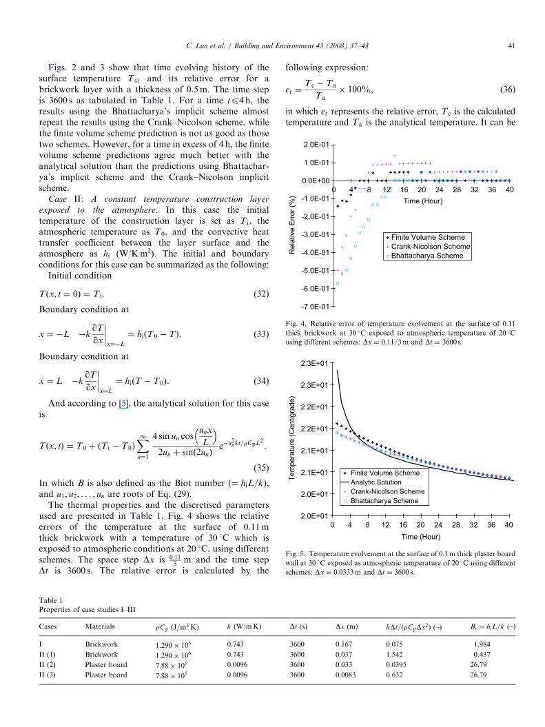
Figs. 2 and 3 show that time evolving history of thesurface temperature T s1 and its relative error for abrickwork layer with a thickness of 0.5m. The time stepis 3600 s as tabulated in Table 1. For a time tp4 h, theresults using the Bhattacharya’s implicit scheme almostrepeat the results using the Crank–Nicolson scheme, whilethe finite volume scheme prediction is not as good as thosetwo schemes. However, for a time in excess of 4 h, the finitevolume scheme predictions agree much better with theanalytical solution than the predictions using Bhattachar-ya’s implicit scheme and the Crank–Nicolson implicitscheme.

Case II: A constant temperature construction layer

exposed to the atmosphere. In this case the initialtemperature of the construction layer is set as T i, theatmospheric temperature as T0, and the convective heattransfer coefficient between the layer surface and theatmosphere as hi (W/Km2). The initial and boundaryconditions for this case can be summarized as the following:

Initial condition

Tðx; t ¼ 0Þ ¼ T i. (32)

Boundary condition at

x ¼ �L �kqT

qx

����x¼�L

¼ hiðT0 � TÞ. (33)

Boundary condition at

x ¼ L �kqT

qx

����x¼L

¼ hiðT � T0Þ. (34)

And according to [5], the analytical solution for this caseis

Tðx; tÞ ¼ T0 þ ðT i � T0ÞX1n¼1

4 sin un cosunx

L

� �2un þ sinð2unÞ

e�u2nkt=rCpL2.

(35)

In which B is also defined as the Biot number ð¼ hiL=kÞ,and u1; u2; . . . ; un are roots of Eq. (29).

The thermal properties and the discretised parametersused are presented in Table 1. Fig. 4 shows the relativeerrors of the temperature at the surface of 0.11mthick brickwork with a temperature of 30 1C which isexposed to atmospheric conditions at 20 1C, using differentschemes. The space step Dx is 0:11

3m and the time step

Dt is 3600 s. The relative error is calculated by the

Table 1

Properties of case studies I–III

Cases Materials rCp ðJ=m3 KÞ k (W/mK)

I Brickwork 1:290� 106 0.743

II (1) Brickwork 1:290� 106 0.743

II (2) Plaster board 7:88� 105 0.0096

II (3) Plaster board 7:88� 105 0.0096

following expression:

er ¼T c � Ta

Ta� 100%, (36)

in which er represents the relative error, T c is the calculatedtemperature and Ta is the analytical temperature. It can be

Dt (s) Dx (m) kDt=ðrCpDx2Þ (–) Bi ¼ hiL=k (–)

3600 0.167 0.075 1.984

3600 0.037 1.542 0.437

3600 0.033 0.0395 26.79

3600 0.0083 0.632 26.79

ARTICLE IN PRESS

2.4E+01

0 4 8 12 16 20 24 28 32 36 40

Time (Hour)

T (

Centigra

de)

dx=L/3

Analytic Solution

dx = L/6

dx=L/12

2.3E+01

2.3E+01

2.2E+01

2.2E+01

2.1E+01

2.1E+01

2.0E+01

2.0E+01

Fig. 6. Effect of different Dx on the predicted temperature profile using

Scheme I ðL ¼ 0:1mÞ.

0.0

5.0

10.0

15.0

20.0

25.0

30.0

0 100

Room

air tem

pera

ture

(C

entigra

de)

Time (hour)

200 300 400 500 600 700 800

Crank-Nicolson schemeFinite volume schemeMeasurements

Fig. 7. Comparisons of the room air temperature obtained by numerical

predictions with the Crank–Nicolson scheme and the finite volume scheme

and by measurements for the cavity brick test module at the University of

Newcastle in December, 2003. The time step is 1 h.

0.0

10.0

20.0

30.0

40.0

50.0

60.0

0

Roof air tem

pera

ture

(C

entigra

de)

Time (Hours from the first day of the month)

100 200 300 400 500 600 700 800

Crank-Nicolson schemeFinite volume method

Measurements

Fig. 8. Comparisons of the roof air temperature obtained by numerical

predictions with the Crank–Nicolson scheme and the finite volume scheme

with the measurements for the cavity brick test module at the University of

Newcastle in December, 2003. The time step is 1 h.

0.0

5.0

10.0

15.0

20.0

25.0

30.0

35.0

0

Tem

pera

ture

of th

e n

ort

h w

all

cavity a

ir (

Centigra

de)

Time (Hours from the first day of the month)

100 200 300 400 500 600 700 800

Crank-Nicolson scheme

Finite volume schemeMeasurements

Fig. 9. Comparisons of the north wall cavity air temperature obtained by

numerical predictions with the Crank–Nicolson scheme and the finite

volume scheme with the measurements for the cavity brick test module at

the University of Newcastle in December, 2003. The time step is 1 h.

C. Luo et al. / Building and Environment 43 (2008) 37–4342

observed from Fig. 4 that the finite volume scheme predictsbetter results than the Crank–Nicolson Scheme and theBhattacharya Scheme for periods t of less than 12h; for t

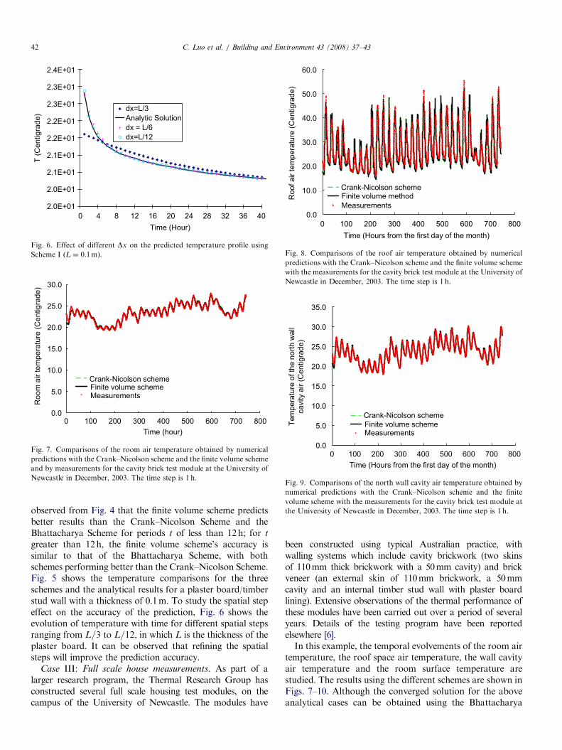
greater than 12h, the finite volume scheme’s accuracy issimilar to that of the Bhattacharya Scheme, with bothschemes performing better than the Crank–Nicolson Scheme.Fig. 5 shows the temperature comparisons for the threeschemes and the analytical results for a plaster board/timberstud wall with a thickness of 0.1m. To study the spatial stepeffect on the accuracy of the prediction, Fig. 6 shows theevolution of temperature with time for different spatial stepsranging from L=3 to L=12, in which L is the thickness of theplaster board. It can be observed that refining the spatialsteps will improve the prediction accuracy.

Case III: Full scale house measurements. As part of alarger research program, the Thermal Research Group hasconstructed several full scale housing test modules, on thecampus of the University of Newcastle. The modules have

been constructed using typical Australian practice, withwalling systems which include cavity brickwork (two skinsof 110mm thick brickwork with a 50mm cavity) and brickveneer (an external skin of 110mm brickwork, a 50mmcavity and an internal timber stud wall with plaster boardlining). Extensive observations of the thermal performance ofthese modules have been carried out over a period of severalyears. Details of the testing program have been reportedelsewhere [6].In this example, the temporal evolvements of the room air

temperature, the roof space air temperature, the wall cavityair temperature and the room surface temperature arestudied. The results using the different schemes are shown inFigs. 7–10. Although the converged solution for the aboveanalytical cases can be obtained using the Bhattacharya

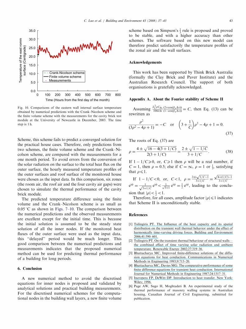
ARTICLE IN PRESS

0.00 700

Tem

pera

ture

of th

e e

ast ro

mm

surf

ace (

Centigra

de)

35.0

30.0

25.0

20.0

15.0

10.0

5.0

Time (Hours from the first day of the month)

100 200 300 400 500 600 800

MeasurementsFinite volume scheme

Crank-Nicolson scheme

Fig. 10. Comparisons of the eastern wall internal surface temperature

obtained by numerical predictions with the Crank–Nicolson scheme and

the finite volume scheme with the measurements for the cavity brick test

module at the University of Newcastle in December, 2003. The time

step is 1 h.

C. Luo et al. / Building and Environment 43 (2008) 37–43 43

Scheme, this scheme fails to predict a converged solution forthe practical house cases. Therefore, only predictions fromtwo schemes, the finite volume scheme and the Crank–Ni-colson scheme, are compared with the measurements for aone month period. To avoid errors from the conversion ofthe solar radiation on the surface to the total heat flux on theouter surface, the hourly measured temperature profiles ofthe outer surfaces and roof surface of the monitored housewere chosen as the input data. In this comparison, six zones(the room air, the roof air and the four cavity air gaps) werechosen to simulate the thermal performance of the cavitybrick module.

The predicted temperature difference using the finitevolume and the Crank–Nicolson scheme is as small as0.05 1C as shown in Figs. 7–10. The comparison betweenthe numerical predictions and the observed measurementsare excellent except for the initial time. This is becausethe initial solution is assumed to be the steady statesolution of all the inner nodes. If the monitored heatfluxes of the outer surface were used as the input data,this ‘‘delayed’’ period would be much longer. Thisgood comparison between the numerical predictions andmeasurements indicates that the proposed numericalmethod can be used for predicting thermal performanceof a building for long periods.

6. Conclusion

A new numerical method to avoid the discretisedequations for inner nodes is proposed and validated byanalytical solutions and practical building measurements.For the discretised numerical schemes for the computa-tional nodes in the building wall layers, a new finite volume

scheme based on Simpson’s 13rule is proposed and proved

to be stable, and with a higher accuracy than otherschemes. The software based on this new model cantherefore predict satisfactorily the temperature profiles ofthe zonal air and the wall surfaces.

Acknowledgements

This work has been supported by Think Brick Australia(formally the Clay Brick and Paver Institute) and theAustralian Research Council. The support of bothorganisations is gratefully acknowledged.

Appendix A. About the Fourier stability of Scheme II

AssumingL2t rCpb

108kDtð2þcosðbxDxÞÞð1�cosðbxDxÞÞ

¼ C, then Eq. (13) can berewritten as

r2

ð3r2 � 4rþ 1Þ¼ �C or 3þ

1

C

� �r2 � 4rþ 1 ¼ 0.

(37)

The roots of Eq. (37) are

r ¼4�

ffiffiffiffiffiffiffiffiffiffiffiffiffiffiffiffiffiffiffiffiffiffiffiffiffiffiffiffiffiffiffiffiffiffi16� 4ð3þ 1=CÞ

p2ð3þ 1=CÞ

¼2�

ffiffiffiffiffiffiffiffiffiffiffiffiffiffiffiffiffi1� 1=C

p3þ 1=C

. (38)

If 1� 1=CX0, or, CX1 then r will be a real number, ifC ¼ 1, then r ¼ 0:5; else if C ¼ 1, r ¼ 1 or 1

3, satisfying

that rp1.

If 1� 1=Co0, or, Co1, r ¼2�i

ffiffiffiffiffiffiffiffiffiffiffi1=C�1p

3þ1=C¼

ffiffiffiffiffiffiffiffiffiffiffiffiffiffiffiffiffi4þð1=CÞ�1p

3þ1=C

eif ¼ 1ffiffiffiffiffiffiffiffiffiffiffi3þ1=Cp eifo 1ffiffiffiffiffiffi

3þ1p eif ¼ 1

2eif, leading to the conclu-

sion that jrjo 12o1.

Therefore, for all cases, amplitude factor jrjp1 indicatesthat Scheme II is unconditionally stable.

References

[1] Tsilingiris PT. The Influence of the heat capacity and its spatial

distribution on the transient wall thermal behavior under the effect of

harmonically time-varying driving forces. Building and Environment

2006;41:590–601.

[2] Tsilingiris PT. On the transient thermal behaviour of structural walls—

the combined effect of time varying solar radiation and ambient

temperature. Renewable Energy 2002;27:319–36.

[3] Bhattacharya MC. Improved finite-difference solutions of the diffu-

sion equations for heat conduction. Communications in Numerical

Methods in Engineering 1993;9:713–20.

[4] Bhattacharya MC, Davies MG. The comparative performance of some

finite difference equations for transient heat conduction. International

Journal for Numerical Methods in Engineering 1987;24:1317–31.

[5] Incropera FP, DeWitt DP. Introduction to heat transfer. New York:

Wiley; 1996.

[6] Page AW, Sugo H, Moghtaderi B. An experimental study of the

thermal performance of masonry walling systems in Australian

housing, Canadian Journal of Civil Engineering, submitted for

publication.