A New Mobility Formula for Spatial Mechanisms

Proceedings of IDETC/CIE 2007ASME 2007 International Design Engineering Technical Conferences &

Computers and Information in Engineering ConferenceSeptember 4-7, 2007, Las Vegas, USA

DETC2007-35574

A NEW MOBILITY FORMULA FOR SPATIAL MECHANISMS

Charles WamplerGeneral Motors R&D Center

30500 Mound Road, MC 480-106-359Warren, Michigan 48090

Email: [email protected]

Blake T. LarsonArthur G. Erdman

Department of Mechanical EngineeringUniversity of Minnesota

Minneapolis, Minnesota 55455Email: [email protected]; [email protected]

ABSTRACTA new formula for predicting the mobility of spatial mecha-

nisms is introduced. Instead of counting rigid links and the con-straints between them, as is done in the usual Grubler-Kutzbachformulae, we count vertices and edges in a polyhedral modelof the mechanism. It is well known that the conventional for-mula underpredicts the mobility of certain exceptional classesof mechanisms, and in particular, does not easily accommodatecompound spatial mechanisms that contain planar or sphericalsub-mechanisms. The new approach provides a correct mobilitywhenever the conventional formula does and accounts for planarand spherical sub-mechanisms in a simple manner. Addition-ally, we present simple modifications to correctly model certainmechanisms that have remote spherical centers. We illustratethe method on compound mechanisms constructed from scissorslinkages.

INTRODUCTIONA necessary step in synthesizing a new mechanism or an-

alyzing a given system is to determine the degrees of freedomof the device. At the outset of designing a mechanism or robotfor a given task or class of tasks, the number of degrees of free-dom of the desired device is specified, and one wishes to explorevarious kinematic topologies to achieve the desired functional-ity. One may also wish to obtain a mechanism with some specialsubset of the space of rigid motions, such as only translationaldegrees of freedom. In this “type synthesis” phase, it is conve-

nient to employ a simple formula, based on a simple accountingof the number of links and the joint types connecting them, topredict the mobility of various linkage topologies under consid-eration. The mobility prediction is equal to the actual degreesof freedom when the link geometries are as general as possiblewithin the assumptions of the accounting method. However, thedegrees of freedom can exceed the mobility index when the linksmeet special conditions. The purpose of this paper is to intro-duce a new mobility formulation that, compared to existing ap-proaches, more easily captures certain special configurations oflinks, thereby providing a tight mobility count for such mecha-nisms. In many cases, more modern refinements of the classicalGrubler-Kutzbach formulae, especially those based on intersec-tion and union of subgroups of the rigid motions, achieve thesame goal. The approach presented here offers an alternativethat seems simpler and more intuitive in many cases. We find itparticularly apt for spatial mechanisms that have multiple centerswhere rotational joints intersect and for compound mechanismsbuilt from scissors linkages.

The most familiar expressions for the mobility M of a spa-tial mechanism of N rigid links with J joints are the Grubler-Kutzbach formulae

M = 6N−6−J

∑j=1

c j =J

∑j=1

f j−6L, (spatial case) (1)

where c j is the number of constraints imposed by joint j, f j isthe number of freedoms allowed by joint j, and L is the num-

1 Copyright c© 2007 by ASME

ber of loop closures [1, 2]. Note that c j + f j = 6. While theserelations are usually attributed to Grubler and Kutzbach, manyothers have contributed to these and offered alternative formula-tions as well [3]. The justification for the first of these formulaebegins with the observation that an unconstrained rigid body inthree-space has 6 degrees of freedom, namely, three translationsand three rotations. Thus, we begin with 6N freedoms, subtractthe total number of constraints imposed by the joints between thelinks, and subtract 6 to declare one of the links as the ground link.(That is, mobility counts the internal degrees of freedom, ignor-ing the rigid body motion of the mechanism as a whole). Thesecond version of the formula recognizes that if we cut L linksto turn the mechanism into an open-tree topology, the resultingmechanism has mobility equal to the sum of the freedoms of itsjoints. It costs 6 degrees of freedom to reconnect each cut link torecover the original mechanism.

It is well-known that the spatial Grubler-Kutzbach formu-lae are incorrect when the joints are in special arrangements. Inparticular, if the mechanism is spherical, that is, if it has onlyrotational joints and these all intersect in a common point, thentranslations can be ignored, and the correct mobility is

M = 3N−3−2J = J−3L, (spherical or planar) (2)

This formula uses the fact that each rotational joint has one de-gree of freedom, or, considering that only orientation is at issue,exerts two constraints. Translation can be ignored in the mobilitycount by placing the world origin and the origin of coordinatesfor each link all at the common intersection point of the joints.With these choices, the translation of every link is identicallyzero. The same formula applies to planar mechanisms, as thesecan be seen to be spherical mechanisms with the common pointat infinity. (Alternatively, one may argue that motion in the planeconsists of two translations and one rotation and thereby arriveat the same formula.) It is not widely recognized, but Eq. 2 actu-ally holds on a somewhat broader class of mechanisms: insteadof requiring all joints to intersect in a common point, it is suffi-cient that all joints meet in a common point for each loop clo-sure. For example, one may use an output angle of one sphericalfour-bar as the input angle to another, and even though the twosub-mechanisms have different spherical centers, Eq. 2 predictsthe correct mobility.

In addition to spherical and planar mechanisms, there existother special arrangements of links. Herve [4] classifies mech-anisms into three categories: “trivial,” for which the Grubler-Kutzbach formulae suffice; “exceptional,” which may have somecombination of intersecting, parallel, and perpendicular jointaxes; and “paradoxical,” in which more complicated relation-ships in the link lengths, twists, and offsets affect the mobil-ity. Examples of the latter include the Bennett four-bar [5] orarchitecturally singular Stewart-Gough platforms [6], whose de-

grees of freedom are higher than the mobility predicted by Eqs. 1or 2. Paradoxical linkages do not submit easily to simple mobil-ity accounting rules as their unexpectedly high degrees of free-dom occur because all the links jointly satisfy one or more extracompatibility conditions. Without a full classification of all suchexceptions, one can only conclude is that the degrees of freedomof a specific mechanism is greater than or equal to the mobility ofthe class of mechanisms to which it belongs. (See Eq. 3 below.)Even this rule has a possible exception, which we discuss below.

One general way to handle “overconstrained” linkages is toform kinematic closure equations and determine the dimensionof their solution set. As the closure equations for many jointtypes, including revolute, prismatic, cylindrical, spherical, andplanar, can be expressed as polynomials, numerical algebraic ge-ometry can be applied to determine the degrees of freedom andto analyze the solution set [7, 8]. However, such a heavy compu-tational procedure is not convenient for the kind of experimenta-tion one might wish to perform during type synthesis. If one isgiven the mechanism in a general configuration, then the co-rankof the Jacobian matrix of the closure equations gives the infinites-imal degrees of freedom of the mechanism. For examples usingthis approach, see [9, 10]. This can be very useful, but it must bekept in mind that there may be fewer finite degrees of freedomthan infinitesimal ones. Also, in linkages having a high degreeof symmetry, it is common that one only knows how to assem-ble the mechanism in a symmetric configuration, which may notbe a general one. For example, it may lie at the intersection ofseveral solution components and therefore have extra infinitesi-mal degrees of freedom. By finding all solution components andtheir dimensions, numerical algebraic geometry overcomes thisdeficiency.

An alternative to a full analysis is to determine how tomodify the Grubler-Kutzbach formulation to correctly accountfor some common exceptions, particularly, to handle compoundmechanisms built by connecting planar, spherical, and spatialsub-mechanisms. Some work in this direction is presentedin [4, 9, 11, 12]

To be more precise about these matters, we must introducesome notations and definitions. Although we know of no excep-tions to the following statements, they lack rigorous proofs, sowe state them as conjectures. More careful statements of theseare contained in [13]. Let X be the set of all mechanisms thathave a given type. Here, type means an enumeration of the links,the types of joints between them, and any extra conditions im-posed on the geometry of the links, such as intersecting jointaxes. Let us assume that these conditions are complex analytic,so that X is an analytic subset of some complex Euclidean space.Let us assume also that all the loop closure equations are complexanalytic, which is true for all joints derived from the lower-orderpairs. (It is not necessarily true for cams and other higher-orderjoints.) Under these assumptions, the solution set of the closureequations, that is, the set of all assembly configurations of the


A

G H

B CD

EF

(a)

A

GH

DC,EB,F

(b)

Figure 1. Mechanism that changes mobility

mechanism, is a complex analytic set. In practice, X is real andwe are only interested in real assembly configurations, but it isadvantageous to first consider the complex case and then restrictto the reals. A particular mechanism, x ∈ X, may have severalassembly modes and these are not necessarily of the same di-mension. For an example, see [7], which shows that a seven-barlinkage built from Roberts cognate four-bars has both a couplercurve and up to six rigid assemblies. From this, we see that themobility of a mechanism can be ambiguous; one should moreproperly speak of the mobility of a mechanism in an assemblymode. Even this can be slippery, for assembly modes of differentdimension may meet, allowing the mechanism to move from onemobility condition to another. This is illustrated by the mech-anism of Fig. 1 built from four triangles and two rigid rectan-gles. If 4AGB =4AGF and 4DHC =4DHE, the configura-tion shown in Fig. 1a, which has mobility one, can be folded flatwhere its mobility increases to two as shown in Fig. 1b since therotations about

−→GB =

−→GF and

−→HC =

−→HE become independent.

For the purposes of this article, we will adopt the conventionthat DOF(x) is the smallest dimension of any assembly mode ofx. We make this choice because we wish to consider a mobilityformula that does not require an assembly configuration to begiven nor do we wish to carry out the calculations needed to findall the assembly modes given just the mechanism description x.Such a formula naturally leads us to the degrees of freedom of thelowest dimensional assembly mode as the other modes involvesome special alignment of joint axes that is evident only given aconfiguration in that mode.

The real degrees of freedom of a mechanism is usually equalto its degrees of freedom in the complexes, but there are excep-tions. Consider a planar four-bar in which the length of onelink is equal to the sum of all the others. It is clear that thiscan be assembled in only one real configuration, with the threeshorter links stretched to exactly span the long one. Over thecomplexes, the loop closure equations have a one-dimensionalsolution set: the real configuration occurs where two branchesof this complex curve intersect. This is analogous to the so-lution set of x2 + y2 = 0, which has only a single real point,(x,y) = (0,0), even though the complex solution set consists oftwo lines, x± yi = 0. Such points are always singular, and a mo-bility analysis based on the co-rank of the Jacobian matrix willindicate, at best, the complex dimension, not the smaller real di-mension.

We must distinguish between two cases: either a generalmember of X can be assembled or not. In the first case, we de-fine the mobility Mob(X), to be the largest integer M such thatthe set U = {x ∈X : DOF(x) = M} is a dense, open subset of X,that is, Mob(X) is the degrees of freedom of a general memberof the type. In the case where a general member cannot be as-sembled, let U be the subset of X that can be assembled as a rigidstructure: U = {x ∈ X : DOF(x) = 0}. Then we define the mo-bility to be Mob(X) = dimU−dimX, that is, the negative of thenumber of extra conditions which must be satisfied to assemblea mechanism of the given type.

From these definitions and the upper-semicontinuity of di-mension, one may see that

DOF(x)≥Mob(X), for all x ∈ X (complex). (3)

It is an immediate consequence that if Y is a subtype of X, i.e.,Y⊂ X, then Mob(Y)≥Mob(X). For this reason, a formula thatcorrectly gives Mob(X) for, say, X equal to the class of spatial6R loops may underpredict the mobility of some special types Yof 6R loops, such as the class of spherical 6R loops. We will saythat a mobility formula F(X) is tight for mechanism type X ifF(X) = Mob(X). A formula that is tight for X may be loose forY⊂ X, meaning F(Y) < Mob(Y).

We emphasize that the preceding paragraph holds only forcomplex degrees of freedom. Letting DOFR(x) be the degreesof freedom (dimension) of the smallest real solution component,we have

DOFR(x)≤ DOF(x). (4)

Unfortunately, this leaves the comparison between DOFR(x) andMob(X) indeterminant in general.

We have the following two conjectures.

Conjecture 1: Equation 1 is tight for spatial mechanism typesgiven only by a list of links and joints.

Conjecture 2: Equation 2 is tight for spherical and planar mech-anism types given only by a list of links and joints. It is alsotight for spatial mechanisms having only rotational joints inwhich each loop closure has a spherical center but the linkparameters are subject to no additional relations.

As stated, these conjectures are not quite true, because wemay have a mechanism that contains an overconstrained sub-mechanism that cannot be assembled while also having sufficientextra degrees of freedom elsewhere to give a total nonnegativemobility. As it is not our purpose here to directly address theseconjectures, we will not burden the exposition with the techni-calities required to rule out such situations.

Our interest in stating these conjectures is to clarify the na-ture of exceptions to Eqs. 1 or 2, namely, any mechanism x ∈ X


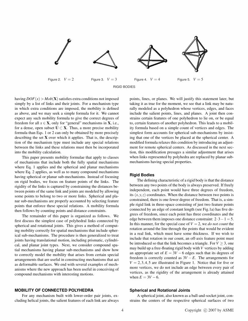
Figure 2. V = 2 Figure 3. V = 3 Figure 4. V = 4 Figure 5. V = 5

RIGID BODIES

having DOF(x) > Mob(X) satisfies extra conditions not imposedsimply by a list of links and their joints. For a mechanism typein which extra conditions are imposed, the mobility is definedas above, and we may seek a simple formula for it. We cannotexpect any such mobility formula to give the correct degrees offreedom for all x ∈ X, only for “general” mechanisms in X, i.e.,for a dense, open subset U ⊂ X. Thus, a more precise mobilityformula than Eqs. 1 or 2 can only be obtained by more preciselydescribing the set X over which it applies. That is, the descrip-tion of the mechanism type must include any special relationsbetween the links and these relations must then be incorporatedinto the mobility calculation.

This paper presents mobility formulae that apply to classesof mechanisms that include both the fully spatial mechanismswhere Eq. 1 applies and the spherical and planar mechanismswhere Eq. 2 applies, as well as to many compound mechanismshaving spherical or planar sub-mechanisms. Instead of focusingon rigid bodies, we focus on feature points of the links. Therigidity of the links is captured by constraining the distances be-tween points of the same link and joints are modeled by allowingsome points to belong to two or more links. Spherical and pla-nar sub-mechanisms are properly accounted by selecting featurepoints that enforce these special relations. A mobility formulathen follows by counting points and distance constraints.

The remainder of this paper is organized as follows. Wefirst discuss the simplest case of polyhedral links connected byspherical and rotational joints. This gives a method of comput-ing mobility correctly for spatial mechanisms that include spher-ical sub-mechanisms. The procedure is then generalized to treatjoints having translational motion, including prismatic, cylindri-cal, and planar joint types. Next, we consider compound spa-tial mechanisms having planar sub-mechanisms and show howto correctly model the mobility that arises from certain specialarrangements that are useful in constructing mechanisms that actas deformable surfaces. We end with several examples of mech-anisms where the new approach has been useful in conceiving ofcompound mechanisms with interesting motions.

MOBILITY OF CONNECTED POLYHEDRAFor any mechanism built with lower-order pair joints, ex-

cluding helical joints, the salient features of each link are always

points, lines, or planes. We will justify this statement later, buttaking it as true for the moment, we see that a link may be natu-rally modeled as a polyhedron whose vertices, edges, and facesinclude the salient points, lines, and planes. A joint then con-strains certain features of one polyhedron to lie on, or be equalto, certain features of another polyhedron. This leads to a mobil-ity formula based on a simple count of vertices and edges. Thesimplest form accounts for spherical sub-mechanisms by insist-ing that one of the vertices be placed at the spherical center. Amodified formula relaxes this condition by introducing an adjust-ment for remote spherical centers. As discussed in the next sec-tion, this modification presages a similar adjustment that ariseswhen links represented by polyhedra are replaced by planar sub-mechanisms having special properties.

Rigid BodiesThe defining characteristic of a rigid body is that the distance

between any two points of the body is always preserved. If freelyindependent, each point would have three degrees of freedom,its (x,y,z) coordinates. When the distance between two points isconstrained, there is one fewer degree of freedom. That is, a sim-ple rigid link in three-space consisting of just two feature pointsconnected by an edge of constant length (see Fig.1a) has five de-grees of freedom, since each point has three coordinates and theedge between them imposes one distance constraint: 2 ·3−1 = 5.In this manner, for the special case of V = 2, we do not count therotation around the line through the points that would be evidentin a real link, which must have some thickness. If we wish toinclude that rotation in our count, an off-axis feature point mustbe introduced so that the link becomes a triangle. For V ≥ 3, onemay build up a free-floating rigid body with V vertices by addingan appropriate set of E = 3V − 6 edges such that its degrees offreedom is correctly counted as 3V −E. The arrangements forV = 2,3,4,5 are illustrated in Figure 1. Notice that for five ormore vertices, we do not include an edge between every pair ofvertices, as the rigidity of the arrangement is already attainedwhen E = 3V −6.

Spherical and Rotational JointsA spherical joint, also known as a ball-and-socket joint, con-

strains the centers of the respective spherical surfaces of two


links to be equal. In the representation of links as polyhedra,this simply means that two bodies share a common vertex. Thisis illustrated in Fig. 6. In Fig. 6a, two triangular-shaped links,labeled “A” and “B”, are joined by a spherical joint at vertexS. Figure 6b represents the polyhedral model, two triangles thatshare vertex S. A minimum of three vertices are required to rep-resent each of these links; otherwise, one of the three rotationalDOF of the spherical joint would be indeterminate. That is, ifpoint 2 did not exist, then rotation about the line segment 1-Scannot be determined, because edges have only one dimension.

(a) SPHERICAL JOINT,TWO LINKS

S

A

B

(b) POLYHEDRAL MODEL(V = 5,E = 6,M = 3)

S

1

2

4

5

Figure 6. SPHERICAL JOINT BETWEEN TWO TRIANGULAR LINKS

A rotational joint is most simply represented in the polyhe-dral model as a pair of distinct points shared by two polyhedra.The rotation axis of the joint is the edge through the vertices.The location of the vertices is not unique, as any two points onthe rotational axis can be chosen.

(a) 2R SPATIAL CHAIN

R16

R26

(b) POLYHEDRAL MODEL(V = 6,E = 10,M = 2)

1

2

3

4

56

R16R26

Figure 7. SPATIAL 2R CHAIN

Figures 7 shows an example of an open 2R chain. Figure 7ashows three links joined at two revolute joints; the general spa-tial case where joints R1 and R2 are skew. Figure 7b shows apolyhedral model of that configuration, and because the rotationaxes are skew the middle link is a tetrahedron. The edge 2-3represents the R1 axis, and edge 4-5 represents the R2 axis.

A spherical sub-mechanism occurs when several rotationaljoints meet in a common point. In Fig. 8, joints R1 and R2 in-tersect at vertex 1, and the middle link becomes a triangle. To

R1CCOR2££±

1V = 5,E = 7,M = 2

Figure 8. SPHERICAL 2R CHAIN

properly account for this, we simply select the common point asone of the two points representing each of the intersecting axes.For parallel joints, the common point is at infinity. For the pur-pose of mobility counting, it is convenient to draw such points asif they are finite, although other notations could be devised, seeFig. 16b. Figure 9 shows a closed-loop 4R spherical four-bar,where four triangles all share a single vertex, 5, with each otheras well as an edge with each neighbor. Note that the four-sidedloop formed by vertices 1-2-3-4-1 is not a rigid body. An addi-tional edge between opposing vertices, either 1-3 or 2-4, wouldreduce the mobility by 1, forming a rigid structure.

1

2 3

4

5V = 5,E = 8,M = 1

Figure 9. SPHERICAL FOUR-BAR POLYHEDRAL MODEL

A Mobility FormulaUsing the ideas of the previous subsections, one can model

any mechanism having only spherical and rotational links as acollection of vertices and edges. Accordingly, the mobility ofthe mechanism is given as

M = 3V −E−6 (5)

As in the first relations of Eqs. 1 and 2, we subtract 6 tofix one link and count only internal degrees of freedom. Usingthis formula for the mechanisms of Figs. 6, 7, 8, and 9 gives thecorrect mobility in all cases. Unlike Eqs. 1 and 2, Eq. 5 holdsfor both spatial and spherical mechanisms.


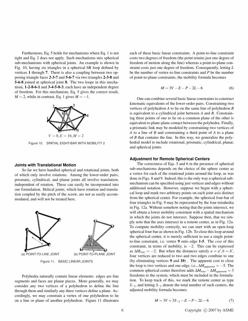
Furthermore, Eq. 5 holds for mechanisms where Eq. 1 is nottight and Eq. 2 does not apply. Such mechanisms mix sphericalsub-mechanisms with spherical joints. An example is shown inFig. 10, having six triangles in a spherical 6R loop defined byvertices 1 through 7. There is also a coupling between two op-posing triangle faces 2-3-7 and 5-6-7 via two triangles 2-3-8 and5-6-8 joined at spherical joint 8. The two loops in this mecha-nism, 1-2-8-6-1 and 3-4-5-8-3, each have an independent degreeof freedom. For this mechanism, Eq. 5 gives the correct result,M = 2, while in contrast, Eq. 1 gives M =−1.

1

2 3

4

56 7

8

V = 8,E = 16,M = 2

Figure 10. SPATIAL EIGHT-BAR WITH MOBILITY 2

Joints with Translational MotionSo far we have handled spherical and rotational joints, both

of which only involve rotations. Among the lower-order pairs,prismatic, cylindrical, and planar joints all involve translation,independent of rotation. These can easily be incorporated intoour formulation. Helical joints, which have rotation and transla-tion coupled by the pitch of the screw, are not as easily accom-modated, and will not be treated here.

QQkQQs

(a) POINT-TO-LINE JOINT

-¾BBM

BBN(b) POINT-TO-PLANE JOINT

Figure 11. BASIC LINEAR JOINTS

Polyhedra naturally contain linear elements: edges are linesegments and faces are planar pieces. More generally, we mayconsider any two vertices of a polyhedron to define the linethrough them and similarly any three vertices define a plane. Ac-cordingly, we may constrain a vertex of one polyhedron to lieon a line or plane of another polyhedron. Figure 11 illustrates

each of these basic linear constraints. A point-to-line constraintcosts two degrees of freedom (the point retains just one degree offreedom of motion along the line) whereas a point-to-plane con-straint costs just one degree of freedom. Consequently, letting Lbe the number of vertex-to-line constraints and P be the numberof point-to-plane constraints, the mobility formula becomes

M = 3V −E−P−2L−6 (6)

One can combine several basic linear constraints to constructkinematic equivalents of the lower-order pairs. Constraining twovertices of polyhedron A to lie on the same line of polyhedron Bis equivalent to a cylindrical joint between A and B. Constrain-ing three points of one to lie on a common plane of the other isequivalent to plane-plane contact between the polyhedra. Finally,a prismatic link may be modeled by constraining two vertices ofA to a line of B and constraining a third point of A to a planeof B that contains the line. In this way, we generalize the poly-hedral model to include rotational, prismatic, cylindrical, planar,and spherical joints.

Adjustment for Remote Spherical CentersThe correctness of Eqs. 5 and 6 in the presence of spherical

sub-mechanisms depends on the choice of the sphere center asa vertex for each of the rotational joints around the loop, as wasdone in Figs. 8 and 9. Indeed, this is the only way a spherical sub-mechanism can be specified using just vertices and edges withoutadditional notation. However, suppose we begin with a spheri-cal loop and mark two arbitrary points on each joint axis distinctfrom the spherical center. For example, the spherical four-bar offour triangles in Fig. 9 may be represented by the four tetrahedrain Fig. 12a. Without somehow noting that the joints intersect, wewill obtain a lower mobility consistent with a spatial mechanismin which the joints do not intersect. Suppose then, that we sim-ply note that the axes intersect in a remote center, as in Fig. 12a.To compute mobility correctly, we can start with an open-loopspherical four-bar as shown in Fig. 12b. To close this loop aroundthe spherical center, it is merely sufficient to use a single point-to-line constraint, i.e. vertex 9 onto edge 1-5. The cost of thisconstraint, in terms of mobility, is −2. This can be expressedas ∆Mtrue = −2. But when the distances satisfy a = a′,b = b′,four vertices are reduced to two and two edges combine to one(by eliminating vertices 9 and 10) . The apparent cost to closethe loop is two vertices and one edge, i.e., ∆Mapparent =−5. Thecommon spherical center therefore adds ∆Mtrue−∆Mapparent = 3freedoms to the system, which must be included in the formula-tion. To keep track of this, we mark the remote center as typeS+3, and letting S+3 denote the total number of such centers, theadjusted mobility formula becomes

M = 3V +3S+3−E−P−2L−6 (7)


1

2

34

5

6

78S+3

(a) CLOSED-LOOP SPHERI-CAL FOUR-BAR

point-to-line

b aa′

b′

1

2 3

45

6 7

89

10(a) OPEN-LOOP SPHERICALFOUR-BAR

Figure 12. SPHERICAL LOOP WITH REMOTE CENTER

We could, of course, do without remote centers and insteadforce a common vertex as in Fig. 9. However, the S+3 terms areincluded as a convenience and in anticipation of additional ad-justment factors needed for other types of mechanisms discussedbelow.

MOBILITY OF CONNECTED SUB-MECHANISMSIn the previous section, we considered mechanisms formed

from polyhedral links connected by joints between points, lines,and planes. Now, suppose we join several such mechanismstogether. One may simply count up the mobility of the wholemechanism using Eq. 7 unless some kind of extra relations existbetween the sub-mechanisms requires an adjustment similar tothe remote center adjustment discussed previously. In this sec-tion, we consider one such class of mechanism that has a partic-ular implementation using planar scissors sub-mechanisms.

Consider a one-degree-of-freedom mechanism that has fouroutput vertices, illustrated schematically in Fig. 13a. Assumethat the motion of the mechanism is such that the four verticesare always coplanar. Therefore the lines through any two pairsof vertices, say line AB and line CD, intersect. Further, assumethere are several such mechanisms connected sequentially as inFig. 13b whose motion characteristics are such that all the indi-cated lines intersect in a common point. Then, we know to checkthe possibility that closing a loop around this common point toform the mechanism of Fig. 13c might, as in the case of remotespherical centers, produce a disparity between the true numberof constraints required to close the loop and the apparent numberimplied by counting vertices. Indeed, if the whole chain of sub-mechanisms is constructed such that the output distances equalthe input distances, i.e., if a = a′,b = b′, then the true cost of clos-ing the loop is ∆Mtrue−2, whereas the apparent cost is two ver-tices, i.e., ∆Mapparent = −6. Therefore, a correct mobility countrequires an adjustment of +4. Accordingly, we mark the remotecenter in this case as type S+4.

1 DOFA

B

C

D

(a) PLANAR SUBMECHANISM

b

a

a′ b′

(b) OPEN CHAIN OF THREE PLANARSUBMECHANISMS

(c) CLOSED CHAIN OF THREE PLANARSUBMECHANISMS

Figure 13. SUBMECHANISMS HAVING A REMOTE CENTER

The situation just described can arise in many ways. Oneis that each of the sub-mechanisms in the series is an identicalsymmetric scissors linkage (see Fig. 14a). If the number of sub-mechanisms is even the conditions are met by identical asym-metrical scissors attached in mirror-image pairs (see Fig. 14b).

A related type of closure is illustrated in Fig. 15, where aseries of sub-mechanisms are connected all sharing a vertex at acommon center. For this configuration, if the design of the sub-mechanisms is such that a = a′, the true cost of closing the loopis again ∆Mtrue = −2, whereas the apparent cost is one vertex,i.e., ∆Mapparent = −3, hence the closure requires an adjustmentof +1. This may be indicated on a diagram of the mechanism asa vertex of type S+1. Similar to above, the condition for a S+1vertex is met by an even number of scissors linkages connectedin mirror-image pairs.

We may account for all such special arrangements by lettingS+k denote the total number of vertices of that type. Accordingly,


(a) CHAIN OF THREE SYMMETRIC SCISSORS

a

b

c

da

b

c

d

(b) FLIPPED PAIR OF ASYMMETRIC SCISSORS

Figure 14. SCISSOR SUBMECHANISMS

Figure 15. THREE SCISSORS WITH A COMMON CENTER

the mobility formula becomes

M = 3V +∑k

kS+k−E−P−2L−6 (8)

This count includes the internal vertices, edges, etc., of the sub-mechanisms. Instead, one can summarize the internal constraintsof each sub-mechanism for the purpose of counting the mobilityof the whole. For example, a scissors mechanism has four ex-posed vertices which contribute 12 to the mobility, but its truecontribution is its internal mobility of 1 plus 6 degrees of free-dom of rigid-body motion, i.e., 7 total. Accordingly, the internalconstraints must add up to -5. So, if we count X scissors sub-mechanisms and their exposed vertices, ignoring their internalvertices and edges, the mobility formula becomes

M = 3V +∑k

kS+k−E−P−2L−5X −6 (9)

One may define similar shortcuts for other types of sub-mechanisms.

A

S B

C

A

B

C

S

Figure 16. PARALLEL-LINK 3CRS MECHANISM

Remark: As a variant on all the preceding formulae, we mayelect to declare one link the immobile ground link, omit any ver-tices of that link from the vertex count V (and omit edges be-tween any two of these), and drop the “−6” from the end of theformula. Counting in this manner, our final formula becomes

M = 3V +∑k

kS+k−E−P−2L−5X (ignoring ground). (10)

EXAMPLESA Translational Mechanism

Consider the parallel-link mechanism shown in Fig. 16a,having three CRS legs meeting at a common spherical centerS. Fixing the ground link, the mechanism has V = 10, E = 15,L = 6, for which Eq. 10 gives mobility M = 3 ·10−15−2 ·6 = 3.Letting vertices A, B, and C move off to infinity, we have themechanism of Fig. 16b having parallel axes. The mechanismstill has three degrees of freedom, but now as point S moves, thelines

−→SA,

−→SB, and

−→SC never change direction. Hence, SABC forms

a rigid frame, shown with bold lines in Fig. 16b, which translatesin three degrees of freedom but does not rotate. A platform linkcan be built on this frame to obtain the translational parallel-linkmechanism due to Tsai [14]. This mechanism is an exceptionallinkage in the Herve classification system.

Spherical Scissors LinkagesConsider any single-loop or multiloop spherical mechanism

built from identical unit links, each subtending the same angle,say α, on the sphere. A rigid binary link may be just one unitlink or it may be constructed by combining equilateral triangles,each with side length α. Tertiary or higher links are also con-structed from such triangles. Now modify the linkage by replac-ing each of the unit links with an identical symmetric scissorslinkage, each rotational joint of the spherical linkage becominga pair of spherical joints as in . For each independent loop of theoriginal mechanism, we have a S+4 remote center. Suppose theoriginal spherical mechanism has M degrees of freedom. The


modified linkage will have M + 1 degrees of freedom; the ex-tra freedom is a simultaneous scissoring of all the unit links,changing α in unison. For example, consider a spherical four-bar. Before modification, it appears as in Fig. 9 with four iden-tical isosceles triangles as sides. It has V = 5, E = 8, and thusM = 3 ·5−8−6 = 1. After modification, it has V = 8, S+4 = 1,X = 4, and thus M = 3 ·8+4−5 ·4−6 = 2. Since the extra de-gree of freedom depends on the identical scissors elements, suchlinkages are paradoxical in the Herve classification.

If the symmetrical scissors have lengths a = b, where a and bare as shown in Fig. 14a, then the external vertices define parallellines, α = 0, even as the scissors operate. The mobility is asbefore, but now the linkage is a planar one that grows and shrinksin the plane as the scissors act.

Collapsible PolyhedraThe Hoberman Sphere is a children’s toy that performs a

dramatic radial expansion from a spiny collapsed shape to a largespherical shape with a single degree of freedom. The key elementof the Hoberman Sphere is a scissor pair designed such that theangle α defined by its exterior points A, B, C, and D remainsthe same as shown in Fig. 17. Such an element may take severalforms [15], and may even consist of multiple scissor pairs joinedin series. The Hoberman-style elements may be connected byspherical joints as shown in Fig. 14 to form various collapsibleshapes. We will use the polyhedral model to compute the mobil-ity of a collapsible cube.

α

A B

CD

E

COLLAPSED ELEMENT

α

A B

D C

E

EXPANDED ELEMENTFigure 17. HOBERMAN-STYLE SCISSOR ELEMENT

A cube is a regular polyhedron with 8 vertices, 12 edges,and 6 faces. To convert this into a Hoberman-style collapsibleobject, we replace each edge with a single DOF sub-mechanism,such as a scissor pair or chain of scissor pairs, that collapse tothe same point. Figure 18a shows how a four-edged cube facecan be replaced by four scissor pairs. The geometry of the scis-sor pair limits the range of motion of the mechanism; we canreplace each single scissor pair with multiply-connected scissorpairs joined by revolute joints as long as the external verticesremain coplanar, maintain the same angle, and maintain equal

input and output distances, that is, |AE|= |BE| and |DE|= |CE|.

(a) FOUR CUBE EDGES REPLACED BY SCISSOR PAIRS

(b) ASSEMBLED COLLAPSIBLE CUBE

Figure 18. COLLAPSIBLE CUBE

Just as three edges meet at each cube vertex, three sub-mechanisms are joined at a “corner” of a collapsible cube (seeFig. 18b). The difference, however, is that the sub-mechanismsmeet at two vertices for each corner. The joints at these cornersare all spherical. Each cube face translates to a closed loop ofsub-mechanisms. In total, there are twelve scissor pairs, each ofwhich could be replaced by a series of scissors. The scissor-pairsare constructed such that the central angle α matches the anglesubtended from the center of a cube by an edge of the cube, thatis α = cos−1(1/3).

To count the mobility of the collapsible cube, first lock allthe scissor pairs such that |AE| = d for some common distanced. Each scissor pair is then equivalent to an identical isoscelestriangle with sides d and apex angle α. These fit together as aset of 9 vertices, the 8 vertices of a cube and its center, joinedby 20 edges, being the 12 edges of a cube plus 8 edges from thecenter to each outer vertex. The mobility of this arrangement is,by Eq. 5, M = 3 · 9− 20− 6 = 1. It can be verified that this isthe correct mobility for a general set of nine vertices connectedby twenty edges in the topological pattern of the cube. How-ever, recall from Eq. 4 that for special mechanisms, the numberof real degrees of freedom can decrease. This indeed happensfor the perfect cube arrangement. Each diagonal of the cubeis exactly spanned by two edges connected at the center. Sim-ilar to the example of the degenerate four-bar with three shortlinks exactly spanning the fourth longer link, the perfect cube isa isolated real point: the mechanism has DOFR = 0 for fixed d.When the scissor pairs are unlocked, the entire collapsible cube


is seen to have mobility DOFR = 1. It is essential that the scis-sor pairs be identical so that as |AE|= d changes, the secondarydistance |DE| also matches on all the scissor pairs. We see thatthe whole mechanism has just one finite real degree of freedom:it expands and contracts. However, the mechanism is singular atevery position, so in addition to the finite motion, it has an extrainfinitesimal motion. Any physical instantiation of it will tend toflex easily in this extra mode. This mechanism could be said tobe doubly paradoxical, as it gains an extra degree of freedom incomplex space due to the special geometry of the Hoberman scis-sors (hence is paradoxical according to Herve), yet in real spaceit loses a degree of freedom as a finite motion in the complexesdegrades to an infinitesimal one in the reals.

A similar analysis can be applied to other collapsible shapes.For a regular tetrahedral shape, which has 4 vertices and 6 edges,replace each of the 6 edges with a scissors pair. ConstructHoberman-type scissor pairs matching the six outer edges andconnect them. With the scissors locked, we have 5 vertices and10 edges for a mobility of M(X) = 3 · 5− 10− 6 = −1. This isthe correct mobility for the mechanism type X consisting of sixtriangles with incompatible central angles; the links cannot gen-erally be assembled in the tetrahedral pattern. However, sincewe have chosen a particular instance, x, having all central anglesequal and compatible with a regular tetrahedron, they do assem-ble, and we have DOFR(x) = DOF(x) = 0 > Mob(X). Hence,the locked-scissors state has mobility zero, while allowing themto unlock gives a mobility M = 1. The collapsible tetrahedronis thus seen to expand and collapse only, always maintaining theshape of a regular tetrahedron.

CONCLUSIONSWe have presented alternatives to the traditional Grubler-

Kutzbach mobility formulae. In the case of just spherical androtational joints, our new formula (Eqn 5) is based on a simplecount of the vertices and edges in a polyhedral model of the as-sembled links. This single formula applies to equally well tospatial, spherical, and planar linkages. We also show how toadapt the formula to include prismatic, cylindrical, and planarjoints, and to correctly count the mobility of certain compoundspatial mechanisms formed by connecting special planar link-ages. This last class of mechanisms includes some collapsiblepolyhedra built with scissors linkages.

We also clarify some subtleties relating to the mobility ofmechanism families. The mobility of a sub-family may be largerthan that of the family containing it, but considering dimensionsin complex space, the mobility never decreases. The real mobil-ity, that is, the dimension of the real solution set of the closureequations, usually is equal to the complex mobility, but in someinstances it may decrease. We illustrate this with an example of acollapsible cube which both gains its collapsible degree of free-dom due to special link geometry (Hoberman scissors) and loses

a degree of freedom into a real singularity.

REFERENCES[1] Grubler, M., 1917. Getriebelehre: eine Theorie des

Zwanglaufes und der ebenen Mechanismen. Springer,Berlin.

[2] Kutzbach, K., 1929. “Mechanische leitungsverzweigung,ihre gesetze und anwendungen”. Maschinenbau, der Be-trieb, 8, pp. 710–716.

[3] Gogu, G., 2005. “Mobility of mechanisms: a critical re-view”. Mechanism and Machine Theory, 40(9), pp. 1068–1097.

[4] Herve, J. M. “Analyse structurelle des mecanismes pargroupe des deplacements”. Mech. Mach. Theory, 13.

[5] Bennett, G. T., 1903. “A new mechanism”. Engineering,76, pp. 777–778.

[6] Husty, M. L., and Karger, A., 2000. “Self-motions ofgriffis-duffy type parallel manipulators”. In Proc. 2000IEEE Int. Conf. Robotics and Automation, p. CDROM.

[7] Sommese, A. J., Verschelde, J., and Wampler, C. W.,2004. “Advances in polynomial continuation for solvingproblems in kinematics”. Journal of Mechanical Design,126(2), pp. 262–268.

[8] Sommese, A. J., and Wampler, C. W., 2005. The NumericalSolution of Systems of Polynomials Arising in Engineeringand Science. World Scientific, Singapore.

[9] Rico, J. M., Gallardo, J., and Ravani, B., 2003. “Lie algebraand the mobility of kinematic chains”. Journal of RoboticsSystems, 20, pp. 477–499.

[10] Rico, J. M., and Ravani, B., 2007. “On calculating the de-grees of freedom or mobility of overconstrained linkages:single-loop exceptional linkages”. J. Mech. Design, 129(3),pp. 310–311.

[11] Zhao, J.-S., Feng, Z.-J., and Dong, J.-X., 2006. “Computa-tion of the configuration degree of freedom of a spatial par-allel mechanism by using reciprocal screw theory”. Mech-anism and Machine Theory, 41(12), 12, pp. 1486–1504.

[12] Hunt, K. H., 1990. Kinematic geometry of mechanisms.Oxford University Press, New York.

[13] Sommese, A. J., and Wampler, C. W., 2007. Mechanismspaces. in preparation.

[14] Kim, H. S., and Tsai, L.-W., 2002. “Evaluation of a carte-sian parallel manipulator”. In Advances in Robot Kinemat-ics, Kluwer Academic Publishers, pp. 21–28.

[15] Patel, J., and Ananthasuresh, G. K., 2006. “A kinematictheory for planar Hoberman and other novel foldable mech-anisms”. In Proc. ASME 2006 Intl. Design Eng. Tech.Conf., ASME, pp. 1–9.


A New Mobility Formula for Spatial Mechanisms

Documents

Transcript of A New Mobility Formula for Spatial Mechanisms