A new hyperbolic model and an experimental study for the flow of polymer melts in Multi-Pass...

This article appeared in a journal published by Elsevier. The attachedcopy is furnished to the author for internal non-commercial researchand education use, including for instruction at the authors institution

and sharing with colleagues.

Other uses, including reproduction and distribution, or selling orlicensing copies, or posting to personal, institutional or third party

websites are prohibited.

In most cases authors are permitted to post their version of thearticle (e.g. in Word or Tex form) to their personal website orinstitutional repository. Authors requiring further information

regarding Elsevier’s archiving and manuscript policies areencouraged to visit:

http://www.elsevier.com/copyright

http://www.elsevier.com/copyright

Author's personal copy

A new hyperbolic model and an experimental study for the flow of polymer meltsin Multi-Pass Rheometer

Amr Guaily a,⇑, Eric Cheluget b, Karen Lee b, Marcelo Epstein a

a Department of Mechanical and Manufacturing Engineering, University of Calgary, Calgary, AB, Canada T2N 1N4b Nova Chemicals Corp., AB, Canada T2E 7K7

a r t i c l e i n f o

Article history:Received 30 December 2009Received in revised form 11 October 2010Accepted 10 January 2011Available online 14 January 2011

Keywords:Viscoelastic liquidsHyperbolic equationsMulti-Pass RheometerFinite element, Boundary conditions

a b s t r a c t

A new mathematical model and an experimental study are presented for polymeric liquids. The mainadvantage of the proposed model over the existing models is its hyperbolic nature, which overcomessome of the drawbacks of the available models. One of the advantages of the proposed model is thatthe boundary conditions can be determined without ambiguity for all variables including the stresses,which may not be the situation for other mixed type systems. The modified Tait equation is used todescribe the polymer compressibility and to keep a real set of characteristics for the resulting systemof equations. The Giesekus model is used to model the polymer viscoelasticity. A hybrid finite ele-ment/finite difference scheme coupled with Newton–Raphson’s linearization scheme is used to solvethe governing system of equations. Numerical and experimental studies for the flow of polymer meltsin a Multi-Pass Rheometer (MPR) are presented. Despite using a one-mode Giesekus model, the predictedshear-rate dependent viscosity curve is in good agreement with the experimental results.

� 2011 Elsevier Ltd All rights reserved.

1. Literature review

1.1. Introduction

Fluids with complex microstructures such as polymers, suspen-sions, and granular materials abound in daily life and in manyindustrial processes in the chemical, food, and oil industries. Themathematical models for flow in such fluids are more complex thanthose of traditional Newtonian fluid dynamics [1]. In this paper, wepresent the results of a numerical and experimental characteriza-tion of a polymeric liquid, an important class of viscoelastic liquids.A viscoelastic liquid is a fluid that exhibits a physical behavior inter-mediate between that of a viscous liquid and an elastic solid. Forthis reason, both the mathematical formulation and the experimen-tal techniques used to describe the response of viscoelastic liquidsare substantially different from their viscous liquid counterparts. Inparticular, the numerical implementation of the governing systemof equations contains important qualitative differences, such asthe character of the equations, the choice of independent variablesand the enforcing of boundary conditions. A comprehensive treat-ment of the associated problems is presented in [2]. It is well knownthat the flow of Newtonian fluids presents a host of mathematical

difficulties. It turns out that all of these difficulties exist also forthe flow of viscoelastic liquids especially at high Weissenberg num-ber besides other sources of numerical difficulties. From a mathe-matical viewpoint, a major difficulty is that the specification ofboundary conditions is connected to the mathematical type of thegoverning equations. General mathematical results are not yetavailable for the case of viscoelastic flows. In particular, the impactof changes of type on the nature of boundary conditions remains tobe analyzed [3]. One of the sources of difficulties in viscoelastic liq-uids is the presence of stress boundary layers and singularities. An-other source of difficulty stems from the convective behavior, andin the treatment of the stress field as a primary unknown, we referto [3] for more details about difficulties in viscoelastic fluids simu-lations. To overcome some of these difficulties, in the present work,we are proposing a purely hyperbolic model. Being a totally hyper-bolic system is of great importance for many reasons, the mostimportant of which are:

I. The boundary conditions can be determined without ambi-guity for all variables including the stresses, which maynot be the situation for other types of systems [4]. Marchaland Crochet [5] proposed a mixed type model, so theychoose the geometry in such a way that the flow is forcedto be fully developed in entry and exit sections, which isnot consistent with the physics of the problem. In our model,we do not have this drawback since the boundary conditionsare determined from the theory of characteristics.

0045-7930/$ - see front matter � 2011 Elsevier Ltd All rights reserved.doi:10.1016/j.compfluid.2011.01.007

⇑ Corresponding author. Current address: Engineering Mathematics and PhysicsDepartment, Cairo University, Giza 12613, Egypt

E-mail addresses: [email protected] (A. Guaily), [email protected] (E.Cheluget), [email protected] (M. Epstein).

Computers & Fluids 44 (2011) 258–266

Contents lists available at ScienceDirect

Computers & Fluids

journal homepage: www.elsevier .com/locate /compfluid


II. A major source of difficulty, which does not exist for our pro-posed model, in numerical simulation for viscoelastic liquidsis the change of type of the system of equations which needsa special numerical treatment to have a stable algorithm asexplained by Joseph [2]. Several investigators [6,7] havelinked the occurrence of a change of type in their numericalschemes to a subsequent loss of convergence. To overcomethis issue, Marchal and Crochet [5] divide the element intoseveral bilinear sub-elements for the stresses, while stream-line-upwinding is used for discretizing the constitutiveequation. The computational complexity of the descretizedproblem is increased significantly by this approach.

III. The stress field is treated as a primary unknown without theneed for a special treatment which is not the case with themixed systems as in [5].

IV. The available hyperbolic numerical algorithms built for tra-ditional Newtonian mechanics could be used without specialtreatment.

Phelan et al. [8] implemented a hyperbolic model but theirresults appear to be very sensitive to the grid discretization andtheir solutions are limited to very coarse spatial discretizations.Guaily and Epstein [9] proposed a unified purely hyperbolic modelfor Maxwell fluids and presented results for compressible andincompressible planar flows.

1.2. Least-squares finite element method (LSFEM)

Least-squares schemes for approximating the solution to differ-ential equations were proposed some time ago as a particular var-iant of the method of weighted residuals. The basic idea is quitestraightforward. Given a trial solution expansion with unknowncoefficients and satisfying the boundary conditions, construct thecorresponding residual for the differential equations. Next, mini-mize the integral mean square residual to generate an algebraicsystem. Finally, solve this algebraic system to determine the coef-ficients and hence the approximation. This approach is appealingbecause the resulting algebraic system is symmetric and positivedefinite for a first-order system of differential equations [10]. Atheoretical analysis of a class of least-squares methods for theapproximate solution of elliptic differential equations was dis-cussed by Varga [11]. Baker [12] obtained error estimates for theleast-squares finite element approximation of the Dirichlet prob-lem for the Laplacian. When compared with the Galerkin finite ele-ment method, least-squares finite element methods generally leadto more stringent continuity requirements for the trial functions.Lynn and Arya [13] and Zienkiewicz et al. [14] demonstrated that

it is possible to reduce the order of continuity requirements atthe expense of introducing more unknowns, by first transformingthe original differential equation into an equivalent system offirst-order differential equations. Subsequently, least-squaresfinite element methods were applied to boundary-layer flow prob-lems [15]. Fix and Gunzburger [16] also studied a least-squaresmethod for systems of first-order equations and applied it to theTricomi equation. A least-squares finite element formulation forthe Euler equations governing inviscid compressible flow was pro-posed by Fletcher [17]. An important feature of his formulation isthe designation of groups of variables rather than single variables.Jiang and Chaig [18] applied the least-squares finite element meth-od to a first-order quasi-linear system for compressible potentialflow. A least-squares collocation finite element method was inves-tigated by Kwok et al. [19] and Carey et al. [20] and applied to tor-sion, plate bending and the Tricomi problem. High order elementswere used for the second-order problem rather than a lower-ordersystem being introduced. More recently, least-squares finite ele-ment methods have received considerable attention in relation totransonic full potential flow calculations and numerical solutionof the Navier–Stokes equations for incompressible viscous flow[21,22]. Carey et al. [23] developed a systematic procedure for con-structing a least-squares finite element method for partial differen-tial equations. The problem is first recast as a first-order systemand the least-squares residual used to form a variational state-ment. Carey et al. [10] described a least-squares mixed finiteelement method and supporting error estimates and briefly sum-marized some computational results for linear elliptic (steadydiffusion) problems. The extension to the stationary Navier–Stokesproblems for Newtonian, generalized Newtonian and viscoelasticfluids is then considered. Pontaza et al. [24] used the approach de-scribed in [23] to solve both the Euler and Navier–Stokes equationsfor the compressible regime. Bolton and Thatcher [25] used theLSFEM to solve the Navier–Stokes equations in the form of stressand stream functions. Gerritsma et al. [26] described a least-squares spectral element formulation in which time stepping wasused to reach steady-state solutions. The time integration methodprovides artificial diffusion which suppresses the oscillations in thevicinity of discontinuities. Ahmadi et al. [27] presented a frame-work and derivations of 2-D higher order global differentiabilityapproximations for 2-D distorted quadrilateral elements whichare widely used with the LSFEM.

1.3. Multi-Pass Rheometer (MPR)

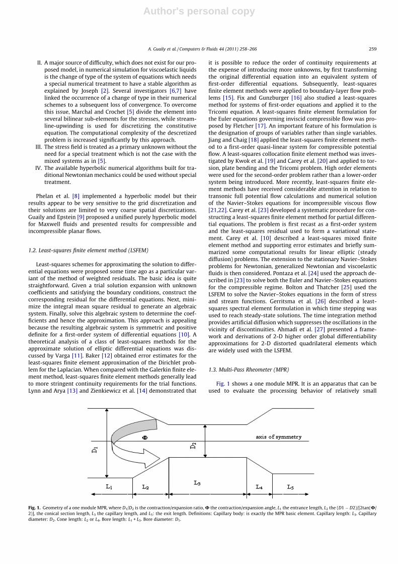
Fig. 1 shows a one module MPR. It is an apparatus that can beused to evaluate the processing behavior of relatively small

Fig. 1. Geometry of a one module MPR, where D1/D2 is the contraction/expansion ratio, U the contraction/expansion angle, L1 the entrance length, L2 the (D1 � D2)/[2tan(U/2)], the conical section length, L3 the capillary length, and L5: the exit length. Definitions: Capillary body: is exactly the MPR basic element. Capillary length: L3. Capillarydiameter: D2. Cone length: L2 or L4. Bore length: L1 + L5. Bore diameter: D1.

A. Guaily et al. / Computers & Fluids 44 (2011) 258–266 259


quantities of molten polymer. The machine has two servo-hydrau-lic controlled speed pistons, and is capable of measuring process-ing performance and generating precise, repeatable results underaccurately controlled flow conditions. The Polymer fluids groupwithin the department of Chemical Engineering, University ofCambridge, has been developing the MPR since 1994. In 1995 theconcept for a twin piston capillary device was proved with MPRMk I which then paved the way for further development workwhich resulted in the construction of MPR II in 1996 [28].

2. Experimental

The MPR is a controlled-strain capillary flow rheometer inwhich the test fluid is vertically displaced back and forth in multi-ple passes. Unlike conventional Instron-type capillary rheometers,the MPR test cell is fully enclosed and tests can be performed athigh temperature and pressure using a small amount of sample.The main MPR operating variables are the piston displacement,temperature and static pressure. The test fluid is displaced througha series of capillaries at a given shear rate (set by the piston speed)and the differential pressure (dP) across each capillary is measured.The temperature and pressure are regulated and monitored bymeans of thermocouples and pressure transducers mounted incylindrical instrumentation modules between each capillary [29].

The viscosity is determined from the shear stress calculatedfrom the measured dP, and the shear rate set by the piston dis-placement. In this paper, the flow in one of the capillaries is mod-eled, and the experimentally measured viscosity curve is comparedwith the simulation results.

3. Governing equations

3.1. Balance laws

Conservation of mass yields the scalar equation

DqDtþ qr � V ¼ 0 ð1Þ

where q denotes the spatial density, V is the velocity field, t denotestime and D/Dt is the material time derivative.

Conservation of momentum yields the vector equation

q@V@tþ qðV � rVÞ ¼ r � s�rpL ð2Þ

where s is the extra stress tensor and pL is the isotropic pressure.The separation of the total stress r into two parts according to:

r ¼ s� pLI ð3Þ

is introduced for later convenience in the expression of the consti-tutive law.

3.2. Constitutive equations

The conservation laws (1) and (2) are not sufficient to deter-mine the unknowns corresponding to the flow. Constitutiveequations are needed to relate the extra stress tensor to the rateof strain tensor. Although many constitutive equations for visco-elastic fluids have been proposed, there is no equation describingcompletely the rheological behavior of viscoelastic fluids. Conse-quently, it is necessary to select a constitutive equation suitablefor numerical analysis with considering fluids and flow fields.Nakamura et al. [30] used seven constitutive equations and calcu-lated the viscosity and the first normal stress coefficient and com-pared them with experimental data. They found that Giesekusmodel is the best differential model that best fit experimental data.Also, it is worth noting that Giesekus model is the only model that

contains a nonlinear term in the stress, representing the Brownianmotion, which makes it more suitable for polymeric liquids. Forthese reasons we will adopt the Giesekus model to describe thepolymer viscoelasticity.

3.2.1. Giesekus modelThe Giesekus model for polymer melts (zero solvent viscosity)

is a three parameter model given by [30]

k@s@tþ ðV � rÞs� ðrVÞs� sðrVÞT

� �þ sþ a

kg0fs � sg ¼ 2g0D

ð4Þ

k is a relaxation time, g0 is the polymer zero-shear-rate viscosity, ais the dimensionless mobility factor (0 6 a 6 1.0).

D ¼ 12ðrV þ ðrVÞTÞ ð5Þ

is the rate of strain tensor.The shear-rate dependent viscosity for the Giesekus model in a

steady shear flow is

gð _cÞ ¼ g0ð1� f Þ2

1þ ð1� 2aÞf

( ); f ¼ 1� v

1þ ð1� 2aÞv ;

v2 ¼ ð1þ 16að1� aÞðk _cÞ2Þ1=2 � 1

8að1� aÞðk _cÞ2ð6Þ

the shear-rate dependent viscosity is defined analogously to the vis-cosity for Newtonian fluids as sxy ¼ gð _cÞ _cxy and _c is the secondinvariant of the rate of strain tensor.

3.3. The compressibility equation

The compressibility effect is accounted for by considering themodified Tait equation [31]

pL ¼ Bqq0

� �c

� 1� �

ð7Þ

where B is a weak function of the entropy (in practice usually takenas a constant), q0 is the liquid density extrapolated to zero pressure,i.e. very nearly the density at 1 atm. Different values for B, q0, and care given in [31].

To transform Eq. (7) into a first-order partial differential equa-tion, we may re-define the isotropic pressure as

p ¼ pL þ B ð8Þ

With the new definition of the pressure; Eq. (7) is exactly thesame, in shape, as the equation of state for perfect gas. Takingthe time derivative for both sides of (7) and using the continuityequation, we get the following equation:

DpDtþ cpðr � VÞ ¼ 0 ð9Þ

The modified Tait equation is used for physical and mathe-matical reasons. The physical reason is to represent the level of li-quid compressibility by the controlling parameter c (the liquid isconsidered incompressible for large values of c), while the mathe-matical reason is to keep the system of equations totally hyperbolicby keeping a real set of characteristics (real eigenvalues, seeSection 6). This could be explained as follows: the property ofthe equation of mass conservation, whereby it behaves as a hyper-bolic equation in the compressible case, it behaves as a constraintequation for the velocity field in the incompressible case. To over-come this difficulty we propose to use the modified Tait equationwith c� 1 in the incompressible limit, which in practice definesan incompressible fluid while keeping a real set of characteristics.

260 A. Guaily et al. / Computers & Fluids 44 (2011) 258–266


4. Nondimensionlization scheme

A major source of numerical difficulties arises from the stan-dard nondimensionalization procedure, especially when simulat-ing compressible fluids at low Mach numbers. Indeed, in thestandard formulation, the free-stream velocity is used to nondi-mensionalize the variables [32], as u� ¼ u

U1; and p� ¼ p

q1U21

, where

(1) refers to free-stream values. With this scaling we see that:

u� ¼ uU1¼ M

1M1

; and p� ¼ p

q1U21¼ p

q1C21

1M21

where C1 is the free-stream speed of sound and Mis the Mach num-ber. For the incompressible limit, M1 goes to zero, which meansthat u⁄ tends to unity while p⁄ tends to infinity. In other words,the pressure term in the momentum equation is of order infinitywhile the advection term is of order unity, which leads to a numer-ical failure due to round-off error in the momentum equation. Thisproblem is more complicated for viscoelastic liquids, as the speed ofsound for air at room temperature is around 330 m/s. Therefore, atsay M1 = 0.3, the speed of the fluid will be approximately 100 m/s.Nevertheless, the speed of sound for compressible liquids is muchlarger than the speed of sound in air (say five times). In applicationssuch as polymer processing, velocity levels are generally low (of theorder of unity [33]). This is why computation of compressible liquidflows is generally associated with much more severe conditionsthan those for gas flows.

To alleviate this problem, in this work we use the free-streamspeed of sound instead of the free-stream velocity as a nondimen-sionalization velocity [34]. The nondimensionalized variablesbecome:

q� ¼ qq1

; V� ¼ VC1

; p� ¼ p

q1C21¼ p

cp1;

s� ¼ s

q1C21; t� ¼ tC1

D1and C2

1 ¼cp1q1

where D1 is the inlet diameter, Henceforth, we will omit the asterisk(�) for clarity.

5. Matrix formulation

In axisymmetric flow and for a unit vector(ey,eh,ex), the velocityvector has the form V = (v,0,u), and the extra stress tensor takesthe form:

s ¼T 0 Q0 E 0Q 0 S

264

375

where ex is a unit vector along the axis of symmetry in Fig. 1 point-ing to the right, ey is a unit vector normal to the axis of symmetry inFig. 1 pointing upward, eh is a unit vector in the tangential directionnormal to the plane of ex and ey, u the velocity in the axial directionex, v the velocity in the normal direction ey, S the stress componentin the axial direction, Q the shear stress, T the stress component inthe normal direction, and E is the stress component in the tangen-tial direction eh.

The velocity gradient is given by

rV ¼

@v@y 0 @v

@x

0 vy 0

@u@y 0 @u

@x

2664

3775

While the divergence of the stress tensor is

r � s ¼ @T@yþ @Q@xþ T � E

y;0;

@Q@yþ @S@xþ Q

y

� �ð10Þ

The system of equations can be written in nondimensional vec-tor form as follows:

At@q@tþ Ax

@q@xþ Ay

@q@y¼ r ð11Þ

The vector of unknowns q = [uvpSQTE]T. The matrix At is theidentity matrix and

Ax ¼

u 0 ðcpÞ�1c �ðcpÞ�

1c 0 0 0

0 u 0 0 �ðcpÞ�1c 0 0

cp 0 u 0 0 0 0

�2 Sþ 1ReWe

� �0 0 u 0 0 0

�Q � Sþ 1ReWe

� �0 0 u 0 0

0 �2Q 0 0 0 u 00 0 0 0 0 0 u

2666666666666664

3777777777777775

and

Ay ¼

v 0 0 0 �ðcpÞ�1c 0 0

0 v ðcpÞ�1c 0 0 �ðcpÞ�

1c0 0

0 cp v 0 0 0 0�2Q 0 0 v 0 0 0

� T þ 1ReWe

� ��Q 0 0 v 0 0

0 �2 T þ 1ReWe

� �0 0 0 v 0

0 0 0 0 0 0 v

2666666666666664

3777777777777775

r ¼ 0 0 0 � SWe� aðS2þQ2Þ

g0� Q

We� aðSQþQTÞ

g0� T

We� aðT2þQ2Þ

g0� E

We� aE2

g0

h iT

The Reynolds number is defined as Re ¼ q1C1D1g0

and the Weissenberg

number as We ¼ kC1D1

, which can be related easily to their regular

definitions using the Mach number M1 ¼ u1C1

, as a scaling factor.

6. Classification of the system of equations

Eq. (11) represents a quasi-linear system of first-order partialdifferential equations. In order to treat such a system numerically,we must first classify it mathematically [8]. The system of Eq. (11)can be classified according to the eigenvalues of the matrix m1 Ax +m2Ay, where m1 and m2 are arbitrary scalars [35]. The rigorouscondition for hyperbolicity requires the matrix m1Ax + m2Ay to havereal eigenvalues for every m1 and m2 [35]. Equivalently, according to[37], the criterion for hyperbolicity for (11) reduces to the require-ment that the matrix Ax or Ay has a full set of real eigenvalues. Thecondition that the matrix Ax has a complete set of real eigenvalues(for arbitrary velocity and stress tensor fields) is both necessaryand sufficient for the system of Eqs. (11) to be fully hyperbolic.For our system of equations (pressure-density based system ofequations), the eigenvalues for Ax are:

k1 ¼ u; k2 ¼ u; k3 ¼ u;

k4 ¼ uþffiffiffiffiffiffiffiffiffiffiffiffiffiffiffiffiffiffiffiffiffiffikðcpÞð�1=cÞ

q; k5 ¼ u�

ffiffiffiffiffiffiffiffiffiffiffiffiffiffiffiffiffiffiffiffiffiffikðcpÞð�1=cÞ

q;

k6 ¼ uþffiffiffiffiffiffiffiffiffiffiffiffiffiffiffiffiffiffiffiffiffiffiffiffiffiffiffiffiffiffiffiffiffiffiffiffiffiffiðcpÞð�1=cÞð2kþ cp

qÞ; k7 ¼ u�

ffiffiffiffiffiffiffiffiffiffiffiffiffiffiffiffiffiffiffiffiffiffiffiffiffiffiffiffiffiffiffiffiffiffiffiffiffiffiðcpÞð�1=cÞð2kþ cp

qÞ

k ¼ Sþ 1ReWe



One can easily show that all of the above eigenvalues are alwaysreal, and consequently, that the system of Eqs. (11) is always purelyhyperbolic under the condition S P �1

ReWe.

7. Numerical algorithm

A hybrid finite element/finite difference scheme coupled withNewton–Raphson’s linearization scheme is used to solve the gov-erning system of equations. Viscoelastic flows remain a demandingclass of problems for approximate analysis, particularly at increas-ing Weissenberg numbers. Part of the difficulty stems from theconvective behavior and in the treatment of the stress field as a pri-mary unknown. This latter aspect has led to the use of higher-orderpiecewise approximations for the stress approximation spaces inrecent finite element research ([38,39]). The computational com-plexity of the descretized problem is increased significantly by this

approach. On the other hand the LSFEM appears to be the most via-ble technique for solving these problems. In addition to the relativeease of its implementation, the LSFEM is a minimization technique,thus is not subject to the LBB (Ladyshenskaya–Babuska–Brezzi)condition and allow us to use equal-order interpolation functionsof all variables which greatly simplify the discretization processwhile the mathematical analysis given in [36] for linear first orderhyperbolic systems shows that Galerkin finite element methodsare formally accurate but unstable [3].

7.1. Time integration scheme

The unsteady term is descritized using a finite difference fullyimplicit backward Euler scheme:

@q@t� Dq

Dt

One has to be carful in choosing the time step as it has a direct effecton the steady-state solution as explained in details in a previouswork [9].

7.2. Linearization scheme

The nonlinear terms may be solved iteratively using Newton–Raphson’s method, by setting:

qnþ1 ¼ qn þ Dq

neglecting the higher order terms. Eq. (11) can be rewritten as:

LDqnþ1 ¼ �f

where

L ¼ Anx@

@xþ An

y@

@yþ 1

DtAt þ An

� �

f ¼ Anx@qn

@xþ An

y@qn

@yþ fnewt

� �

7.3. Space integration scheme: LSFEM

We start by defining the residual vector to be minimized overthe computational domain [34] as

E ¼ LDqnþ1 þ f ð12Þ

the least squares functional is given by:

JðDqnþ1Þ ¼ 12

Z ZXðEÞTðEÞdX ð13Þ

Minimizing (13) yields the least squares weak form as:Z ZXðLNÞTðLDqnþ1 þ fÞdX ¼ 0 ð14Þ

We can now introduce the finite element approximation as:

Dqnþ1 � Dqnþ1h ¼

Xne

j¼1

NjDqnþ1j ð15Þ

where ne is the number of nodes per element and Nj (j = 1, . . . ,ne) arethe element shape functions

A ¼

@u@x

@u@y �ðcpÞ�

cþ1c @p

@x � @S@x�

@Q@y �

Qy

� �0 �ðcpÞ�

1c

y 0 0

@v@x

@v@y �ðcpÞ�

cþ1c @p

@y� @T@y �

@Q@x � T�E

y

� �0 0 �ðcpÞ�

1c

yðcpÞ�

1c

y

@p@x

@p@y þ

cpy c @u

@x þ @v@y þ v

y

� �0 0 0 0

@S@x

@S@y 0 1

We� 2 @u

@x þ 2aSRe �2 @u@x þ 2aQRe 0 0

@Q@x

@Q@y 0 � @v

@x þ aQRe1

We� @u

@x � @v@y þ aðSþ TÞRe � @u

@y þ aQRe 0@T@x

@T@y 0 0 �2 @v

@x þ 2aQRe1

We� 2 @v

@y þ 2aTRe 0@E@x

@E@y 0 0 0 0 1

We� 2 v

y þ 2aERe

2666666666666666664

3777777777777777775

fnewt ¼ �ðcpÞ�1c Q

y

� ��ðcpÞ�

1c T�E

y

� �cpv

yS

Weþ aReðS2 þ Q 2Þ Q

Weþ aReðSQ þ QTÞ T

Weþ aReðT2 þ Q 2Þ E

Weþ aReE2 � 2Ev

y � 2vyReWe

h iT

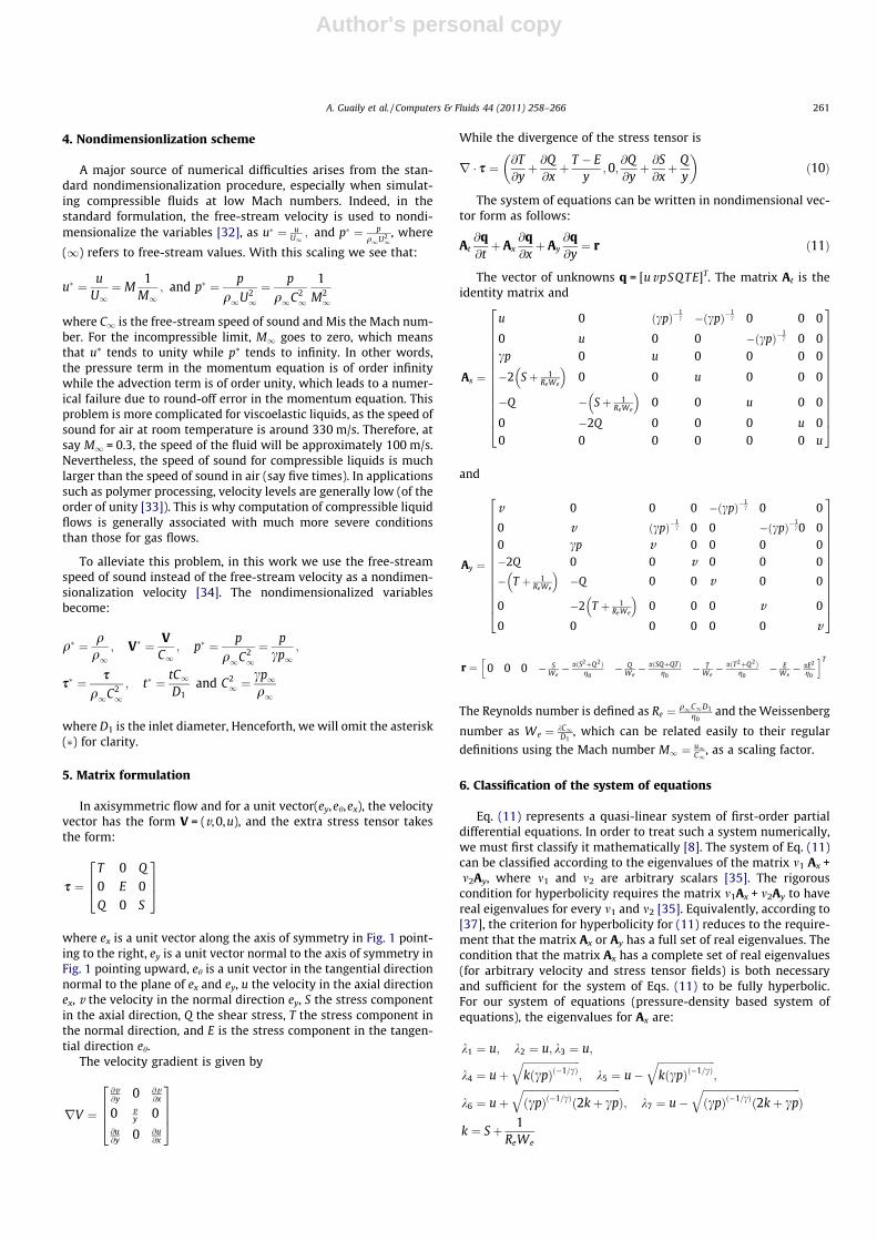
Fig. 2. Geometry and grid.



Introducing the finite element approximation (15) into Eq. (14)results in the linear algebraic system of equations:

½K�fDqg ¼ �fRg ð16Þ

where Keij ¼

R RXe ðLNiÞTðLNjÞdXe; re

i ¼R R

Xe ðLNiÞT fdX are evaluatedusing Gauss–Legendre quadrature.

8. Boundary conditions

For a hyperbolic system of equations, considerations on charac-teristics show that one must be cautious about prescribing the

solution on the boundary. In some particular cases, the boundaryconditions can be found by physical considerations (such as a solidwall), but their derivation in the general case is not obvious. Theproblem of finding the ‘‘correct’’ boundary conditions, i.e., thosewhich lead to a well-posed problem, is difficult in general fromboth the theoretical and practical points of view (proof of well-posedness, choice of the physical variables that can be prescribed).The correct number and type of boundary conditions to be im-posed on a boundary is determined by the theory of characteristicsaccording to the incoming/outgoing characteristics. For the math-ematical details we refer to [4]. In the finite element method, theboundary conditions are easily imposed, a fact that can be consid-ered as one of the most important features of the finite elementmethod.

9. Numerical simulation

9.1. Nearly viscoelastic limit

9.1.1. Fluid, Flow and Geometric Data

a ¼ 0:001; c ¼ 7:15; M1 ¼ 0:0001; Re ¼ 0:001; We ¼ 0:001;D1

D2¼ 9

5; U ¼ 90; L1 ¼ L3 ¼ 5

Fig. 2 shows the geometry and the grid used in the simulation for

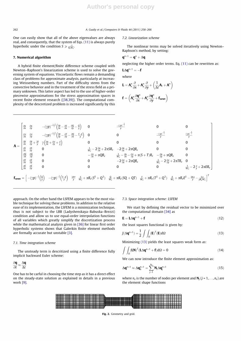
Fig. 3. Velocity isocontours.

Fig. 4. The pressure and the density isocontours.

Fig. 5. Shear stress isocontours.



the MPR.Computations were performed with (Dt = 0.05). The grid con-

sists of 132 X 10 bi-linear quadrilateral elements, corresponds toa number of unknowns of 10,241. With 10 elements in the y-direc-tion, 30 uniformly distributed elements on the capillary section L3,50 elements uniformly distributed in the entrance section L1, 40clustered (using a geometric series) elements for the exit sectionL5 and 6 uniformly distributed elements for each conical section.The initial guess for the Newton–Raphson’s scheme is zero every-

where for the velocities and the stresses and for the pressure; thefree-stream value is used everywhere.

Applying the theory of characteristics [4], the boundary condi-tions at the inlet are1:

u ¼ 4M1ð1� y2Þ; v ¼ 0; S ¼ 2We

Re

@u@y

� �2

; T ¼ 0; E ¼ 0

At the exit, the boundary conditions are p ¼ 1=c; Q ¼ 1Re

@u@y.

The no-slip boundary condition is imposed on the outer bound-ary. As well as the symmetry conditions are imposed.

The variables plotted in the following figures are nondimen-sionalized as

u� ¼ uU1

; v� ¼ vU1

; p� ¼ pp1

; s� ¼ s

q1U21

The first N1p and the second N2p principal stress differences are de-fined as

N1p ¼ ½ðS� TÞ2 þ 4Q 2�1=2; N2p ¼

Sþ T2þ 1

2½ðS� TÞ2 þ 4Q2�1=2 � E

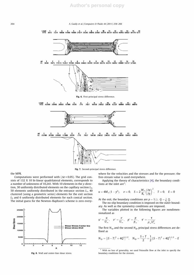
Fig. 6. First-principal stress difference.

Fig. 7. Second-principal stress difference.

Fig. 8. Wall and center-line shear stress.

1 With no loss of generality, we used Poiseuille flow at the inlet to specify theboundary conditions for the stresses.



Fig. 3 shows the axial (top) and radial (bottom) velocity isocontoursfor the MPR, as expected and from experimental observations forcreeping weakly viscoelastic (Newtonian Limit), no vortex formedin the contraction/expansion zones and the maximum velocity ob-tained in the capillary section. Fig. 4 shows the pressure (top) andthe density (bottom) isocontours, one conclusion form this figureis that the flow is mainly incompressible as the maximum density

variation is 0.1% which is less than the limit for compressible flows(5%) which means that adopting the Tait equation to keep thehyperbolic nature by keeping a real set of characteristics does notpractically affect the problem physics. Also there is almost no pres-sure loss across the capillary which is consistent with the experi-mental observations.

Fig. 5 shows the shear stress isocontours, the symmetry of theflow is observed easily in this figure. Also as expected, there isno high gradient for the stress beside the wall as we are simulatingthe Newtonian limit (low Weissenberg number) flow. The sameconclusions can be obtained form the isocontours of the first-and second-principal stress difference shown in Figs. 6 and 7respectively.

One of the most important flow results is the wall shear stressshown in Fig. 8. For comparison, the shear stress at the center lineis presented as well. As seen in the figure, the wall shear stress in-creases in the capillary section so one can get higher shear rates toenable the measurement the shear-rate dependant viscosity.

Fig. 9 shows the velocity distribution at the exit section com-pared to the one at the inlet. One can notice that we get a fullydeveloped flow distributions at the exit section, which reflectsone of the most important advantages of having a hyperbolic mod-el, namely we only impose the pressure and one stress componentin the tangential direction at the exit boundary as determined fromthe theory characteristics. In the mixed type models [5], one has toimpose non-physical boundary conditions to force the flow to befully developed at the exit. The first/second-principal stress differ-ence distributions at both the inlet and exit section are plotted inFig. 10.

It is worth mentioning that a mesh refinement test was done ina previous work [9], in which we model planar flow problems,smaller size problems.

9.2. Viscoelastic analysis

For the polymer melt used in the experiment, the Tait equationexponent is c = 3.09, the Giesekus model parameters are: themobility factor a = 0.009; the relaxation time is k = 0.01 [s] andthe flow parameters are Re = 0.0013; We = 0.0333 based on a pistonspeed of 30 mm/s and polymer density of q1 = 759 kg/m3. The flowis considered to be isothermal. The boundary conditions formulasused in the previous analysis is used again here with the new val-ues mentioned above for the Reynolds and Weissenberg numbers.Fig. 11 (top) shows the geometry and the grid used in the simula-tion; a clustered grid is used to capture the high stress and velocitygradients. Also shown in Fig. 11 (middle) are the resulting axial

Axial Velocity

Rad

ius

0 0.2 0.4 0.6 0.8 10

0.25

0.5

InletOutlet

Fig. 9. Velocity distribution at the inlet/exit.

Principal Stress Difference

Rad

ius

0 2000 4000 6000 80000

0.25

0.5

1st Principal stress Diff. Inlet1st Principal stress Diff. outlet2nd Principal stress Diff. inlet2nd Principal stress Diff. outlet

Fig. 10. Principal stress difference at the inlet/exit section.

Fig. 11. Grid and velocity isocontours for the MPR.



velocity isocontours; as expected, the velocity reaches its maxi-mum inside the capillary without any circulation in/out of the cap-illary zone as can be seen in streamlines plot in Fig. 11 (bottom).The shear-rate dependant viscosity is plotted in Fig. 12 for boththe experimental and numerical simulations. As seen in the figure,the numerical results agree well with the experimental results de-spite using a one-mode Giesekus model.

10. Conclusions

Numerical and experimental investigations of viscoelastic liq-uids are presented. A one module MPR is used to carry out theexperiments. The theoretical formulation permits the governingequations to be cast in the form of a totally hyperbolic system offirst-order PDEs. The pure hyperbolic nature of the model over-comes some of the drawbacks of available models. The mostimportant of these drawbacks is the mixed nature of the resultingsystems of equations, with the subsequent consequence of havingno general numerical algorithm for the solution as well as there isno clear way to know the correct number and type of boundaryconditions to be imposed on a boundary to get a well-posed prob-lem which is not the case for hyperbolic systems. A hybrid least-squares finite element/finite difference scheme coupled with aNewton–Raphson’s algorithm is used to solve the resulting systemof equations. The Tait equation was used for two reasons (1) phys-ically: to account for the polymer compressibility. (2) Mathemati-cally: to keep a real set of characteristics, as has been shown by theeigenvalues, so as to have a purely hyperbolic system everywherein the computational domain. The Giesekus model was used to de-scribe the liquid viscoelasticity. We suggest using a multi-modeGiesekus model to get more accurate representation for liquid vis-coelasticity and to use more than one capillary module to get high-er shear rates.

Acknowledgement

This work has been supported in part by the Natural Sciencesand Engineering Research Council of Canada (NSERC).

References

[1] Renardy M. Mathematical analysis of viscoelastic flows. In: CBMS-NSF regionalconference series in applied mathematics, no. 73; 2000.

[2] Joseph D. Fluid dynamics of viscoelastic liquids. Applied mathematical science,vol. 84. New York: Springer-Verlag; 1990.

[3] Keunings R. Progress and challenges in computational rheology. Rheol Acta1990;29:556–70.

[4] Godlewski E, Raviart PA. Numerical approximation of the hyperbolic systemsof conservation laws. Applied mathematical Sciences, vol. 118. NewYork: Springer-Verlag; 1996.

[5] Marchal JM, Crochet MJ. A new mixed finite element for calculatingviscoelastic flow. J Non-Newton Fluid Mech 1987;26:77–114.

[6] Brown RA, Armstrong RC, Beris AN, Yeh PW. Galerkin finite element analysis ofcomplex viscoelastic flows. Comput Meth Appl Mech Eng 1986;58:201–26.

[7] Song JH, Yoo JY. Numerical simulation of viscoelastic flow through a suddencontraction using a type dependent difference method. J Non-Newton FluidMech 1987;24:221–43.

[8] Phelan Jr FR, Malone MF, Winter HH. A purely hyperbolic model for unsteadyviscoelastic flow. J Non-Newtonian Fluid Mech 1989;32:197–224.

[9] Guaily A, Epstein M. A unified hyperbolic model for viscoelastic liquids. MechRes Commun 2010;37:158–63.

[10] Carey GF, Pehlivanov AI, Shen Y, Bose A, Wang KC. Least-squares finiteelements for fluid flow and transport. Int J Numer Meth Fluids1998;27:97–107.

[11] Varga RS. Functional analysis and approximation theory in numerical analysis.In: Regional conference series in applied mathematics, no. 3, SIAM,Philadelphia; 1971.

[12] Baker G. Simplified proofs of error estimates of the least squares method forDirichlet’s problem. Math Comput 1973;27:229–35.

[13] Lynn PP, Arya SK. Use of the least squares criterion in the finite elementformulation. Int J Numer Methods Eng 1973;6:75–88.

[14] Zienkiewicz OC, Owen DRJ, Lee KN. Least squares finite element for elasto-static problems-use of reduced integration. Int J Numer Methods Eng1974;8:341–58.

[15] Lynn PP, Alani K. Efficient least squares finite elements for two-dimensionallaminar boundary layer analysis. Int J Numer Methods Eng 1976;10:809–25.

[16] Fix GJ, Gunzburger MD. On least squares approximations to indefiniteproblems of the mixed type. Int J Numer Methods Eng 1978;12:453–69.

[17] Fletcher CAJ. A primitive variable finite element formulation for inviscidcompressible flow. J Comput Phys 1979;33:301–12.

[18] Jiang BN, Chai J. Least squares finite element analysis of steady high subsonicplane potential flows. Acta Mech Sin 1980:90–3.

[19] Kwok WL, Cheung YK, Delcourt C. Application of least squares collocationtechnique in finite element and finite strip formulation. Int J Numer MethodsEng 1977;11:1391–404.

[20] Carey GF, Cheung YK, Lau SL. Mixed operator problems using least squaresfinite element collocation. Comput Meth Appl Mech Eng 1980;22:121–30.

[21] Bristeau MO, Glowinski R, Periaux J, Perrier P, Pironneau O. On the numericalsolution of nonlinear problems in fluid dynamics by least squares and finiteelement methods. I – least square formulations and conjugate gradientsolution of the continuous problems. Comput Meth Appl Mech Eng 1979;17/18:619–57.

[22] Bristeau MO, Pironneau O, Glowinski R, Périaux J, Perrier P, Poirier G. On thenumerical solution of nonlinear problems in fluid dynamics by least squaresand finite element methods (II). Application to transonic flow simulations.Comput Meth Appl Mech Eng 1985;51:363–94.

[23] Carey GF, Jiang BN. Least-squares finite element method andpreconditioned conjugate gradient solution. Int J Numer Methods Eng1987;24:1283–96.

[24] Pontaza JP, Diao Xu, Reddy JN, Surana KS. Least-squares finite element modelsof two-dimensional compressible flows. Finite Elem Anal Design2004;40:629–44.

[25] Bolton P, Thatcher RW. A least-squares finite element method for the Navier–Stokes equations. J Comput Phys 2006;213:174–83.

[26] Gerritsma M, Bas R, Maerschalck B, Koren B, Deconinck H. Least-squaresspectral element method applied to the Euler equations. Int J Numer MethFluids 2008;57:1371–95.

[27] Ahmadi A, Surana KS, Maduri RK, Romkes A, Reddy JN. Higher order globaldifferentiability local approximations for 2-D distorted quadrilateral elements.Int J Comput Meth Eng Sci Mech 2009;10:1–19.

[28] http://www.cheng.cam.ac.uk/research/groups/polymer/MPR/.[29] Mackley MR, Spittler P. Viscoelastic characterisation of polyethylene using a

multipass rheometer. Rheol Acta 1996;35:202–9.[30] Nakamura K, Mori N, Yamamoto T. Examination of constitutive equations for

polymer solutions. J Textile Mach Soc Jpn Trans 1992;45(5):T71–9.[31] Thompson PA. Compressible fluid dynamics. New York: McGraw-Hill; 1972.[32] Moussaoui F. A unified approach for inviscid compressible and nearly

incompressible flow by least-squares finite element method. Appl NumerMath 2003;44:183–99.

[33] Keshtiban IJ, Belblidia F, Webster MF. Computation of incompressible andweakly-compressible viscoelastic liquids flow: finite element/volumeschemes. J Non-Newton Fluid Mech 2005;126:123–43.

[34] Taghaddosi F, Habashi WG, Guevremont G, Ait-Ali-Yahia D. An adaptive least-squares method for the compressible euler equations. Int J Numer Meth Fluids1999;31:1121–39.

[35] Courant R, Hilbert D. Methods of mathematical physics, vol. 2. NewYork: Wiley; 1962.

[36] Johnson C, Navert U, Pitkaranta J. Finite element methods for linear hyperbolicproblems. Comput Meth Appl Mech Eng 1984;45:285–312.

[37] Brian J, Antony N. Remarks concerning compressible viscoelastic fluid models.J Non-Newton Fluid Mech 1990;36:411–7.

[38] Baaijens FPT. Mixed finite element methods for viscoelastic flow analysis: areview. J Non-Newton Fluid Mech 1998;79:361–85.

[39] Guenette R, Fortin M. A new mixed finite element method for computingviscoelastic flows. J Non-Newton Fluid Mech 1995;60:27–52.

Fig. 12. Viscosity versus shear rate.


A new hyperbolic model and an experimental study for the flow of polymer melts in Multi-Pass...

Documents

Transcript of A new hyperbolic model and an experimental study for the flow of polymer melts in Multi-Pass...