A new compact scheme for parallel computing using domain decomposition
24
A new compact scheme for parallel computing using domain decomposition T.K. Sengupta * , A. Dipankar, A. Kameswara Rao Department of Aerospace Engineering, I.I.T. Kanpur, U.P. 208016, India Received 16 January 2006; received in revised form 17 May 2006; accepted 22 May 2006 Available online 18 July 2006 Abstract Direct numerical simulation (DNS) of complex flows require solving the problem on parallel machines using high accu- racy schemes. Compact schemes provide very high spectral resolution, while satisfying the physical dispersion relation numerically. However, as shown here, compact schemes also display bias in the direction of convection – often producing numerical instability near the inflow and severely damping the solution, always near the outflow. This does not allow its use for parallel computing using domain decomposition and solving the problem in parallel in different sub-domains. To avoid this, in all reported parallel computations with compact schemes the full domain is treated integrally, while using parallel Thomas algorithm (PTA) or parallel diagonal dominant (PDD) algorithm in different processors with resultant latencies and inefficiencies. For domain decomposition methods using compact scheme in each sub-domain independently, a new class of compact schemes is proposed and specific strategies are developed to remove remaining problems of parallel computing. This is calibrated here for parallel computing by solving one-dimensional wave equation by domain decom- position method. We also provide the error norm with respect to the wavelength of the propagated wave-packet. Next, the advantage of the new compact scheme, on a parallel framework, has been shown by solving three-dimensional unsteady Navier–Stokes equations for flow past a cone-cylinder configuration at a Mach number of 4. Additionally, a test case is conducted on the advection of a vortex for a subsonic case to provide an estimate for the error and parallel efficiency of the method using the proposed compact scheme in multiple processors. Ó 2006 Elsevier Inc. All rights reserved. Keywords: Compact schemes; Domain decomposition method; Parallel computing; DNS 1. Introduction For parallel computing, domain decomposition method of Schwartz [1,2] is preferred in either its multipli- cative or additive variations [3] – where a complex large problem is solved in smaller sub-domains indepen- dently and exchanging overlap region data or information among conjoint sub-domains. While the original Schwartz method uses overlapping sub-domains – this is inefficient in parallel computing procedures due to various latencies of processes caused by interprocessor communications among sub-domains, specially for 0021-9991/$ - see front matter Ó 2006 Elsevier Inc. All rights reserved. doi:10.1016/j.jcp.2006.05.018 * Corresponding author. Fax: +91 512 590007/597561. E-mail address: [email protected] (T.K. Sengupta). Journal of Computational Physics 220 (2007) 654–677 www.elsevier.com/locate/jcp
Transcript of A new compact scheme for parallel computing using domain decomposition
Journal of Computational Physics 220 (2007) 654–677
www.elsevier.com/locate/jcp
A new compact scheme for parallel computing usingdomain decomposition
T.K. Sengupta *, A. Dipankar, A. Kameswara Rao
Department of Aerospace Engineering, I.I.T. Kanpur, U.P. 208016, India
Received 16 January 2006; received in revised form 17 May 2006; accepted 22 May 2006Available online 18 July 2006
Abstract
Direct numerical simulation (DNS) of complex flows require solving the problem on parallel machines using high accu-racy schemes. Compact schemes provide very high spectral resolution, while satisfying the physical dispersion relationnumerically. However, as shown here, compact schemes also display bias in the direction of convection – often producingnumerical instability near the inflow and severely damping the solution, always near the outflow. This does not allow itsuse for parallel computing using domain decomposition and solving the problem in parallel in different sub-domains. Toavoid this, in all reported parallel computations with compact schemes the full domain is treated integrally, while usingparallel Thomas algorithm (PTA) or parallel diagonal dominant (PDD) algorithm in different processors with resultantlatencies and inefficiencies. For domain decomposition methods using compact scheme in each sub-domain independently,a new class of compact schemes is proposed and specific strategies are developed to remove remaining problems of parallelcomputing. This is calibrated here for parallel computing by solving one-dimensional wave equation by domain decom-position method. We also provide the error norm with respect to the wavelength of the propagated wave-packet. Next,the advantage of the new compact scheme, on a parallel framework, has been shown by solving three-dimensionalunsteady Navier–Stokes equations for flow past a cone-cylinder configuration at a Mach number of 4.
Additionally, a test case is conducted on the advection of a vortex for a subsonic case to provide an estimate for theerror and parallel efficiency of the method using the proposed compact scheme in multiple processors.� 2006 Elsevier Inc. All rights reserved.
Keywords: Compact schemes; Domain decomposition method; Parallel computing; DNS
1. Introduction
For parallel computing, domain decomposition method of Schwartz [1,2] is preferred in either its multipli-cative or additive variations [3] – where a complex large problem is solved in smaller sub-domains indepen-dently and exchanging overlap region data or information among conjoint sub-domains. While the originalSchwartz method uses overlapping sub-domains – this is inefficient in parallel computing procedures due tovarious latencies of processes caused by interprocessor communications among sub-domains, specially for
0021-9991/$ - see front matter � 2006 Elsevier Inc. All rights reserved.
doi:10.1016/j.jcp.2006.05.018
* Corresponding author. Fax: +91 512 590007/597561.E-mail address: [email protected] (T.K. Sengupta).
T.K. Sengupta et al. / Journal of Computational Physics 220 (2007) 654–677 655
multiplicative Schwartz method (MSM) as compared to additive Schwartz method (ASM) [3] in parallel com-puting. Larger the size of overlap region, more problematic it becomes for parallel computing, as it involveslarger data transfer among nodes. Thus, this overlapping region is removed in many variants where the non-overlapping sub-domains interact with their neighbors via interface boundary condition(s) only. The non-overlapping domains are also preferred when the grids are non-matching in contiguous sub-domains.
To remedy the slowness of convergence of the Schwartz’s method, Lions [4] proposed to replace Dirichletinterface conditions by Robin interface conditions and the parameters of the artificial boundary conditions(ABC) were obtained via optimization for faster convergence rate. The resultant convergence rate is functionof the parameters of ABC and on the amount of overlap among sub-domains. The latter actually increasesconvergence exponentially for CFD problems governed by convection and diffusion operators, when the flowis normal to the interface and the time step is small. For large time steps and when flow is tangential to theinterface then this type of exponential convergence is absent. This information helps in the decision of decom-posing the given flow domain and would be used in our examples. Also, the non-overlapping sub-domainssuffer from poor convergence for high wave number components of the error [3]. It is to be noted that theconvergence properties of Schwartz’s method are critical for parabolic and elliptic PDEs and not so significantfor hyperbolic or propagation problems.
Most parallel computations are performed using explicit formulations to avoid problems of passing volumeof data among various sub-domains that becomes mandatory for implicit methods. Shang et al. [5] and Loc-kard and Morris [6] have reported efficient parallel explicit algorithms for multi-physics problems. While someefforts have been made in [7] towards developing parallel codes using high accuracy compact schemes, accord-ing to these authors efficient implementation of compact schemes on parallel computers remains an open problem.Basic compact schemes [8] have enormous advantages of large spectral resolution as compared to high orderexplicit schemes and hence preferred, whenever possible. It has also been shown in [9,10] that compact schemeswith appropriate time integration schemes help preserve the physical dispersion relation in numerical sense –known as the dispersion relation preservation (DRP) property, that is mandatory for DNS. However,compact schemes with its associated one-sided boundary closure schemes (ABC) gives rise two inconvenientfeatures of these methods. Firstly, a large number of often-used compact schemes have numerical instabilityproblems near the inflow of the domain. Secondly, near the outflow, compact schemes give rise to massiveattenuation of the function. In [9], a matrix-stability analysis method was introduced that quantitatively iden-tified these shortcomings of compact schemes. The authors also provided newer compact schemes that avoidthe above numerical instability problems. This peculiarity of compact schemes gives the solution a distinct biasto the procedure. When compact schemes are used in an integral domain, the ensuing instability is not persis-tent as the disturbance propagates downstream where the scheme has a stable behavior. However this will notbe the case when the domain is segmented in the streamwise direction. Thus, this prohibits usage of compactschemes in individual sub-domains – where the solutions will display nonphysical growth and attenuation nearthe sub-domain interfaces for convection dominated phenomenon. This property will be demonstrated by awave propagation problem solved in segmented overlapping domains. We will also suggest various meansto overcome this problem. All earlier attempts where conventional compact schemes have been used, the flowdomain is treated integrally, while various solution methods involved in compact schemes are computed in adistributed fashion.
This is done by performing various operations associated with obtaining derivatives, integrals and/or filter-ing operation via distributed computing. In most of these cases one is required to solve linear algebraic equa-tions simultaneously. For the often-used compact schemes, this requires solving banded tridiagonal matrixequations by Thomas algorithm that requires O(N) operations for N unknowns. In [7] pipelined implementa-tion of the Thomas algorithm (PTA) is discussed where various latencies of processors are reduced by per-forming non-local data-independent computations, solving for other spatial derivatives during forward andbackward operations in PTA. Alternative to PTA is discussed in [11,12], where newer algorithms are proposedthat replaces the forward and backward recursions of PTA by matrix-vector multiplications. However, thisleads to significant increase in floating-point operations, defeating the rationale of faster computing byparallelization.
In another alternative a parallel diagonal dominant (PDD) algorithm was proposed in [13] for solvingToeplitz tridiagonal system arising from the usage of compact schemes. As the PDD algorithm is necessarily
656 T.K. Sengupta et al. / Journal of Computational Physics 220 (2007) 654–677
an approximation, the enhanced accuracy of compact schemes is compromised, in addition to incurring highercomputational effort as compared to PTA.
In all parallel implementations referred to above, computations are done by solving the problem togetherby executing PTA or PDD algorithm in different processors, that imposes latencies and inefficiencies of com-putations. The above discussion raises the possibility to consider a strategy where one splits the full probleminto multiple sub-domains and use Schwartz’s method – eliminating all the problems of PTA and PDD algo-rithms, provided one can remove the unphysical bias of compact schemes. This can be attempted by a largeoverlap of contiguous sub-domains- since it has been established in [3] that the application of Schwartz’smethod via domain decomposition will have little or no problems of convergence if the overlap is sufficientlylarge. Such overlap of sub-domains are also required, as the analysis of [9] indicates that the problematic biasof traditional compact schemes exist over the first and last six to seven nodes in the domain. However, thiswould mean additional repetitive computations over twelve to fourteen nodes in every sub-domain. It wouldbe preferable if the number of overlapping nodes can be reduced significantly. In a recent effort [14], a newcompact scheme has been introduced that removes the asymmetry of basic compact schemes, in solving thesub-critical instability problem of plane Poiseuille flow that requires obtaining very high accuracy symmetricequilibrium solution. In the present research, a new class of symmetrized compact schemes is establishedfurthermore by designing and using two such unbiased schemes to: (a) solve a wave propagation problem;(b) solve three-dimensional unsteady Navier–Stokes equation for high Mach number supersonic flow(M1 = 4.0) past a cone-cylinder configuration; and (c) convection of a vortex governed by inviscid equationsfor subsonic Mach number (M1 = 0.4). It should however, be pointed out that while the bias of compactschemes can be minimized – it cannot be completely removed. In such a situation, a Schwartzian domaindecomposition may still give rise to numerical problems for parallel computing near the interfaces thatrequires detailed investigation. In the present work, we want to reduce the overlap to a minimum, so thatan efficient parallelization is made possible. Apart from the usage of larger overlap of contiguous sub-domainsto reduce numerical problems in parallel computing, we also propose here to use filtering in the physical space[15] or adding artificial numerical dissipation to remove the same problems.
The paper is formatted in the following manner. In the next section a new symmetrized compact scheme isdeveloped. The developed scheme is tested for the propagation of a wave-packet following the one-dimen-sional wave equation. This will help establish the numerical properties of the developed symmetrized compactscheme for its stability and dispersion relation preservation property with respect to different parallelizingstrategy using domain decomposition method. We also show the effects of physical plane filters in controllingsome numerical problems of parallel computing. In Section 3, we use a symmetrized scheme to solve the three-dimensional supersonic flow at M1 = 4.0 past a cone-cylinder assembly by solving the unsteady three-dimen-sional Navier–Stokes equation. To test the ability of the proposed method for elliptic problems, we have stud-ied the convection of a shielded vortex in inviscid flow at M1 = 0.4 in Section 4. The paper closes with someconclusions in Section 5.
2. Development of a symmetrized compact scheme for parallel computing
It is well known that compact difference schemes [8,9] used for solving PDEs possess very high spectralaccuracy in resolving various spatial scales. For CFD and many other related activities, these schemes are usedto evaluate various derivatives in an implicit manner. For example, to evaluate first derivatives u 0 of a vectoru(xj), j = 1, . . .,N one can write it down as,
½A�fu0g ¼ ½B�fug: ð1Þ
While this representation is valid for both explicit (with A as an identity matrix) and implicit methods, anequivalent explicit representation of this general form can be written down as,fu0g ¼ 1
h½C�fug ð2Þ
where h is the uniform grid spacing used for discretizing the domain. However, one does not work with C
matrix while using compact schemes. Many practical problems require non-periodic boundary conditions
T.K. Sengupta et al. / Journal of Computational Physics 220 (2007) 654–677 657
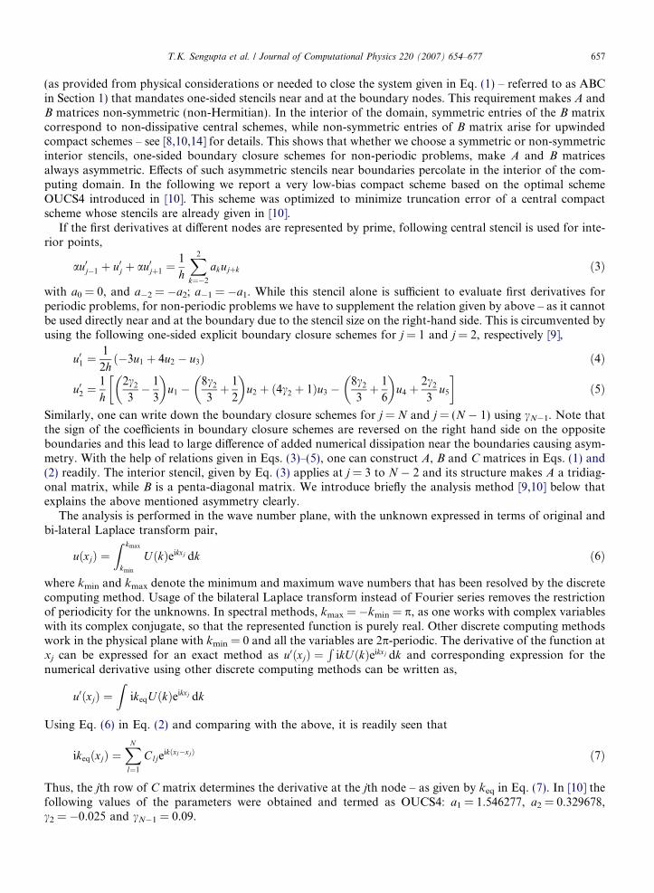
(as provided from physical considerations or needed to close the system given in Eq. (1) – referred to as ABCin Section 1) that mandates one-sided stencils near and at the boundary nodes. This requirement makes A andB matrices non-symmetric (non-Hermitian). In the interior of the domain, symmetric entries of the B matrixcorrespond to non-dissipative central schemes, while non-symmetric entries of B matrix arise for upwindedcompact schemes – see [8,10,14] for details. This shows that whether we choose a symmetric or non-symmetricinterior stencils, one-sided boundary closure schemes for non-periodic problems, make A and B matricesalways asymmetric. Effects of such asymmetric stencils near boundaries percolate in the interior of the com-puting domain. In the following we report a very low-bias compact scheme based on the optimal schemeOUCS4 introduced in [10]. This scheme was optimized to minimize truncation error of a central compactscheme whose stencils are already given in [10].
If the first derivatives at different nodes are represented by prime, following central stencil is used for inte-rior points,
au0j�1 þ u0j þ au0jþ1 ¼1
h
X2
k¼�2
akujþk ð3Þ
with a0 = 0, and a�2 = �a2; a�1 = �a1. While this stencil alone is sufficient to evaluate first derivatives forperiodic problems, for non-periodic problems we have to supplement the relation given by above – as it cannotbe used directly near and at the boundary due to the stencil size on the right-hand side. This is circumvented byusing the following one-sided explicit boundary closure schemes for j = 1 and j = 2, respectively [9],
u01 ¼1
2hð�3u1 þ 4u2 � u3Þ ð4Þ
u02 ¼1
h2c2
3� 1
3
� �u1 �
8c2
3þ 1
2
� �u2 þ ð4c2 þ 1Þu3 �
8c2
3þ 1
6
� �u4 þ
2c2
3u5
� �ð5Þ
Similarly, one can write down the boundary closure schemes for j = N and j = (N � 1) using cN�1. Note thatthe sign of the coefficients in boundary closure schemes are reversed on the right hand side on the oppositeboundaries and this lead to large difference of added numerical dissipation near the boundaries causing asym-metry. With the help of relations given in Eqs. (3)–(5), one can construct A, B and C matrices in Eqs. (1) and(2) readily. The interior stencil, given by Eq. (3) applies at j = 3 to N � 2 and its structure makes A a tridiag-onal matrix, while B is a penta-diagonal matrix. We introduce briefly the analysis method [9,10] below thatexplains the above mentioned asymmetry clearly.
The analysis is performed in the wave number plane, with the unknown expressed in terms of original andbi-lateral Laplace transform pair,
uðxjÞ ¼Z kmax
kmin
UðkÞeikxj dk ð6Þ
where kmin and kmax denote the minimum and maximum wave numbers that has been resolved by the discretecomputing method. Usage of the bilateral Laplace transform instead of Fourier series removes the restrictionof periodicity for the unknowns. In spectral methods, kmax = �kmin = p, as one works with complex variableswith its complex conjugate, so that the represented function is purely real. Other discrete computing methodswork in the physical plane with kmin = 0 and all the variables are 2p-periodic. The derivative of the function atxj can be expressed for an exact method as u0ðxjÞ ¼
RikUðkÞeikxj dk and corresponding expression for the
numerical derivative using other discrete computing methods can be written as,
u0ðxjÞ ¼Z
ikeqUðkÞeikxj dk
Using Eq. (6) in Eq. (2) and comparing with the above, it is readily seen that
ikeqðxjÞ ¼XN
l¼1
Cljeikðxl�xjÞ ð7Þ
Thus, the jth row of C matrix determines the derivative at the jth node – as given by keq in Eq. (7). In [10] thefollowing values of the parameters were obtained and termed as OUCS4: a1 = 1.546277, a2 = 0.329678,c2 = �0.025 and cN�1 = 0.09.
658 T.K. Sengupta et al. / Journal of Computational Physics 220 (2007) 654–677
Asymmetric behavior of compact schemes can be clearly noted from Eq. (7) due to the asymmetric C
matrix. The reason for the asymmetry of C is due to one-sided boundary closure schemes given by Eqs. (4)and (5). Symmetrization of C matrix can be brought about by either of two methods. In the first methodwe simply take an arithmetic average of the entries of C matrix in Eq. (2) about the center row (that representsthe middle of the domain), thereby making the derivative symmetric and removing the bias of the compactscheme. This was suggested and followed in [14]. There is the second method where we evaluate the derivativesusing Eq. (1) at all nodes by going from j = 1 to N and going from j = N to 1 in each sub-domain. The sym-metrized derivative are taken as the average of the derivatives obtained in following these two directions.While these two alternative procedure of symmetrizing the derivatives are identical, in the first procedureone performs N2 multiplications and in the second process this involves solving Thomas algorithm twice,thereby performing 10N operations. Thus, if one chooses N > 10, the second method is faster, and such achoice of N is always made to avoid the negative effects of boundary closure schemes. We will refer to thismethod of evaluating derivatives as the S-OUCS4 scheme in the rest of the paper. It is important to investigatethat apart from removing the bias of compact schemes, whether the new scheme retains or improves thenumerical properties, the amplification rate and DRP. These properties are studied here with respect to themodel one-dimensional linear convection equation that represents many convective flows and wavephenomena,
ouotþ c
ouox¼ 0; c > 0 ð8Þ
Eq. (8) is non-dispersive and convects the initial solution to the right with speed c i.e. the group velocity isequal to the phase speed c. This equation helps study numerical instability and most importantly the disper-sion error and DRP property [9,14], using physical and numerical group velocity. It is necessary to ensure thatthe numerical group velocity is as close to the physical group velocity as possible for the resolved space-timescales. This is discussed next along with the numerical stability of space-time discretization schemes for Eq.(8).
Consider the numerical solution of Eq. (8) subject to the following initial condition,
u0m ¼ uðxm; t ¼ 0Þ ¼
ZA0ðkÞeikxm dk ð9Þ
The exact solution of Eq. (8) can be written down in terms of the initial solution as,
uexactðx; tÞ ¼Z
A0ðkÞeikðx�ctÞ dk ð10Þ
The numerical solution can be represented at x = xm and t = tn by unm ¼
R bU ðk; tnÞeikxm dk, so that a numerical
amplification factor can be introduced by GðkÞ ¼ bU ðk;tnþ1ÞbU ðk;tnÞ.
One can compare the exact solution with that obtained numerically by using Eq. (9) in discretized Eq. (8) toobtain general numerical solution [10] as,
unm ¼ uðxm; tnÞ ¼
ZA0ðkÞðG2
r þ G2i Þ
n=2eikðxm�nbÞ dk ð11Þ
where the numerical amplification factor is given by G(k) = Gr(k) + iGi(k) and tanb = �Gi/Gr. The numericalgroup velocity is found from the numerical dispersion relation as given by [10],
V gN ðkÞc¼ 1
N chdbdk
ð12Þ
where Nc = cDt/h is the CFL number.For non-periodic problems, the corresponding quantities will vary from node to node. If for a discrete com-
puting scheme the spatial derivative at the jth node is evaluated using Eq. (7), then it is given by,
ouj
ox¼ 1
h
XN
l¼1
Cljeikðxl�xjÞuj ð13Þ
T.K. Sengupta et al. / Journal of Computational Physics 220 (2007) 654–677 659
Utilizing this in Eq. (8) one gets
ouj
otþ cuj
h
XClj½cos kðxl � xjÞ þ i sin kðxl � xjÞ� ¼ 0 ð14Þ
This equation can be used to obtain wave-number dependent amplification factor at the jth node, Gj(k), oncethe time integration method is fixed. We have used the four-stage Runge–Kutta (RK4) time integration strat-egy here, as it was noted to have good numerical stability and DRP property [14], when used with traditionalcompact schemes. The amplification factor for the RK4 time integration scheme, for jth node can be shown tobe given by [14]:
Gjðkh;N cÞ ¼ 1� Aj þA2
j
2�
A3j
6þ
A4j
24ð15Þ
where
Aj ¼ N c
XN
l¼1
Cljeikðxl�xjÞ ð16Þ
Using Eqs. (15) and (16), one obtains the amplification factors at all spatial nodes for any combinations of kh
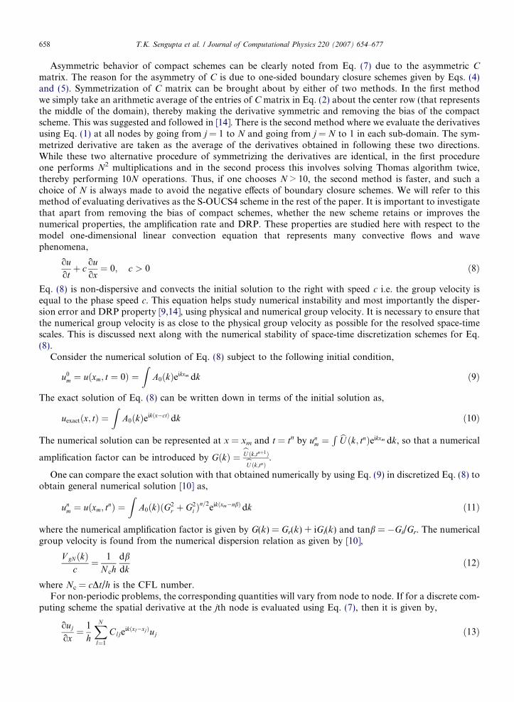
and Nc for RK4 time integration scheme. In the above, we can use the symmetrized C matrix by replacing theentries of the jth and (N � j + 1)th rows of the C matrix by their arithmetic average, where N is the number ofpoints. Such symmetrizing operation will also alter the above discussed numerical properties. In Fig. 1, jGjj atdifferent representative nodes are shown by taking N = 101. On the left column of Fig. 1, shown are the ampli-fication rate contours for the jth node and on the right corresponding results for (N � j + 1)th nodes for theoriginal OUCS4 method. In the middle column of Fig. 1, corresponding results are shown for the S-OUCS4scheme at the same nodes. Results for j = 2 exhibit unstable nature, even for very small values of Nc, while forj = 100 we note excessive damping for the OUCS4 scheme. In contrast, S-OUCS4 method has significantlyimproved amplification rates for j = 2 and (N � 1). Similar improvements have been brought about at allnear-boundary points. It is seen that there is negligible asymmetry of jGj for j P 8 onwards for the basicOUCS4 scheme that is removed by symmetrization.
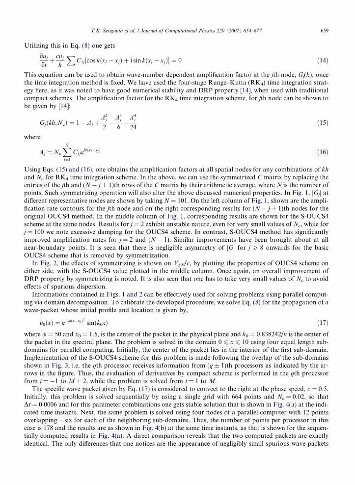
In Fig. 2, the effects of symmetrizing is shown on VgN/c, by plotting the properties of OUCS4 scheme oneither side, with the S-OUCS4 value plotted in the middle column. Once again, an overall improvement ofDRP property by symmetrizing is noted. It is also seen that one has to take very small values of Nc to avoideffects of spurious dispersion.
Informations contained in Figs. 1 and 2 can be effectively used for solving problems using parallel comput-ing via domain decomposition. To calibrate the developed procedure, we solve Eq. (8) for the propagation of awave-packet whose initial profile and location is given by,
u0ðxÞ ¼ e�/ðx�x0Þ2 sinðk0xÞ ð17Þ
where / = 50 and x0 = 1.5, is the center of the packet in the physical plane and k0 = 0.838242/h is the center ofthe packet in the spectral plane. The problem is solved in the domain 0 6 x 6 10 using four equal length sub-domains for parallel computing. Initially, the center of the packet lies in the interior of the first sub-domain.Implementation of the S-OUCS4 scheme for this problem is made following the overlap of the sub-domainsshown in Fig. 3, i.e. the qth processor receives information from (q ± 1)th processors as indicated by the ar-rows in the figure. Thus, the evaluation of derivatives by compact scheme is performed in the qth processorfrom i = �1 to M + 2, while the problem is solved from i = 1 to M.The specific wave packet given by Eq. (17) is considered to convect to the right at the phase speed, c = 0.5.Initially, this problem is solved sequentially by using a single grid with 664 points and Nc = 0.02, so thatDt = 0.0006 and for this parameter combinations one gets stable solution that is shown in Fig. 4(a) at the indi-cated time instants. Next, the same problem is solved using four nodes of a parallel computer with 12 pointsoverlapping – six for each of the neighboring sub-domains. Thus, the number of points per processor in thiscase is 178 and the results are as shown in Fig. 4(b) at the same time instants, as that is shown for the sequen-tially computed results in Fig. 4(a). A direct comparison reveals that the two computed packets are exactlyidentical. The only differences that one notices are the appearance of negligibly small spurious wave-packets
0.950.95
0.950.95
11
1
1
1
1
1.051.05
1.05
1.051.05
5
5
5
5
100
100
100
Nc
kh
1 2 3 4 5 6
1
2
3
4
5
6
j = 2 (a)
0.95
0.95
0.95
0.95
0.95
0.95
0.950.95
0.95
0.95
1 1
1
1
11
1
11
1
1.05
1.05
1.051.05
1.05
1.05
5
5
5
5
5
100
10
100
10
Nc
kh
1 2 3 4 5 6
1
2
3
4
5
6
j = 2,100 (b)
0.95
0.95
0.95
0.950.95
0.95
0.95
0.95
0.95
1 1
1
11
1
1 1
1.05
1.051.05
1.05
5
5
5
5
10
100100
Nc
kh
1 2 3 4 5 6
1
2
3
4
5
6
j = 100 (c)
0.95
0.95
0.95
0.95
0.95
0.95
0.95
1 1
1
1
1
1
1
11
1.05
1.05
1.05
1.05
1.05
5
5
5
5
100
100
Nc
kh
1 2 3 4 5 6
1
2
3
4
5
6
j = 3
0.95
0.95
0.95
0.95
0.95
0.95
0.95
0.95
0.95
1
1
1
1
1
11
1.05
1.05
1.05
1.05
5
5
5
5
100
100
100
Nc
kh
1 2 3 4 5 6
1
2
3
4
5
6
j = 4
0.95
0.95
0.95
0.95
0.95
0.95
0.95
0.95
0.95
1
1
1
11
1
11
1.05
1.05
1.05
1.05
1.05
5
5
5
5
5
100
100
100
100
100
Nc
kdx
1 2 3 4 5 6
1
2
3
4
5
6
j = 5
0.95
0.95
0.95
0.95
0.95
0.95 0.950.95
0.95
0.950.95
0.950.95
0.95
11
1
1 1
1
1
1 111
1
1 1
11
1
1
1.05
1.05
1.051.05
1.05
1.05
5
5
5 55
5
100
100100
100
100
Nc
kdx
1 2 3 4 5 6
1
2
3
4
5
6
j = 50
0.95
0.95
0.95
0.95
0.95
0.95
0.95 0.950.95
0.95
0.95
1
1 11
1
11
1
1
1
1 1
1.05
1.051.051.05
1.05
1.05
5
55
5
5
5
100
100
100
100
Nc
kh
1 2 3 4 5 6
1
2
3
4
5
6
j = 4, 98
0.950.95
0.95
0.95
0.95
0.95
0.950.950.95
0.95
0.95
0.95
0.95
0.95
11
1
1
1
1
1 111
1
1 1
11
1
1.05
1.05
1.05 1.051.05
1.05
1.05
5
5
5 55
5
100
100
100
100
Nc
kdx
1 2 3 4 5 6
1
2
3
4
5
6
j = 50, 52
0.950.95
0.95
0.95
0.95
0.95
0.95
0.95
0.95
0.95
1 1
1
1
11
1
1
1 1
1.05
1.05
1.05
1.05
1.05
1.05
5
5
55
5
5
100
100
Nc
kh
1 2 3 4 5 6
1
2
3
4
5
6
j = 3, 99
0.95
0.95
0.95
0.95
0.95
0.95
0.95
0.95
1 1
1
1
1
1 1
1.05
1.05
1.05
1.05
5
5
5
5
100
100
Nc
kh
1 2 3 4 5 6
1
2
3
4
5
6
j = 99
0.950.
95
0.95
0.95
0.95
0.95
095 0.95
1
1
1
1
1
1
1
1
1
1.05
1.05
1.05
1.05
1.05
1.05
5
5
5
5
5
100
100
100
100
Nc
kh
1 2 3 4 5 6
1
2
3
4
5
6
j = 98
0.95
0.95
0.95
0.95
0.95
0.95
0.950.95
0.95
1
1
1
11
1
1
1
1 1
1.05
1.05
1.051.05
1.05
1.05
1.05
5
5
55
5
5
100
100100
100
10
Nc
kdx
1 2 3 4 5 6
1
2
3
4
5
6
j = 97
0.95
0.95
0.95
0.95
0.95
0.95
0.95 0.90.95
0.95
0.95
0.95
0.95
0.95
11
1
1
1
1
1 111
1
1
1
1
1
1.05
1.05
1.05 1.05
1.05
1.05
5
5 55
5
5
100
100
10100
100
100
Nc
kdx
1 2 3 4 5 6
1
2
3
4
5
6
j = 52
0.95
0.95
0.95
0.95
0.95
0.95
0.950.95
0.95
0.95
1 1
1
1
1
1
1
1
1
1
1 1
1.05
1.05
1.05 1.051.05
1.05
1.05
5
5
55
5
5
100
100100
100
Nc
kdx
1 2 3 4 5 6
1
2
3
4
5
6
j = 5, 97
Fig. 1. Amplification factor (jGj) contours in (kh-Nc)-plane for (a), (c) OUCS4 and (b) S-OUCS4 at the indicated nodes.
660 T.K. Sengupta et al. / Journal of Computational Physics 220 (2007) 654–677
-1
-1 -1
0
0 0
0.95
0.95
0.95
0.95
0.95
0.95
1
1
1
1
1
11
11 1
1.05
1.05
1.05
1.05
1.05
1.051.051.05
Nc
kdx
1 2 3 4 5 6
1
2
3
4
5
6
j = 50
-1
-1-1
0
0
0
0
0.95
0.95
0.9
11
1
1
1
1
1
1
1
1.05
1.05
1.05
1.051.05
1.05
Nc
kdx
1 2 3 4 5 6
1
2
3
4
5
6
j = 2 (a)
-1 -1
-1-1
00
00
0.95 0.95
0.95
0.95
0.95
0.95
0.95
1
1
1
1 1
1
1
1
1.05
1.05
1.05
1.051.05
1.05
Nc
kdx
1 2 3 4 5 6
1
2
3
4
5
6
j = 3
-1
-1-1
-1
0
0
00 0
0.95
0.95
0.95 0.95
1
1
1
1
1 1
1
0.95
1
1
1.05
1.05
1.05
1.05
1.05
1.051.05
1.05
1.05
Nc
kdx
1 2 3 4 5 6
1
2
3
4
5
6
j = 4
-1-1
-1 -1
0 0
0 0
0.95
0.95
0.95
0.95
0.95
0.95
0.95
11
11
1
-1
11
11
1.05
1.05
1.05
1.05
1.0
1.05
1.051.05
Nc
kdx
1 2 3 4 5 6
1
2
3
4
5
6
j = 5
-1
-1
-1
0
0
0
0.950
1.05
0.95
0.95
0.95
0.95
1
1
1
1
11
1
1
1
1
1
1
1
1.05
1.05
1.05
1.05
1.05
1.05
1.05
1.05
1.05
Nc
kdx
1 2 3 4 5 6
1
2
3
4
5
6
j = 100 (c)
-1
-1
0
0
0.95
0.95
0.95
0.950.95
0.95
0.95
0.95
0.95
1
11
1
1
1
1
1
1
1
1 1
1.05
1.05
1.05
1.05
1.05
1.05
1.05
1.05
1.05
1.05
1.05
Nc
kdx
1 2 3 4 5 6
1
2
3
4
5
6
j = 99
-1
0
00
0
0
0
0
0.95 0.95
0.950.95
0.95
0.95 0.95
1
1
1
11
11
1
1
1
1
1.01.05
1.05
1.05
1.05
1.051.05
1.05
1.05
1.05
Nc
kdx
1 2 3 4 5 6
1
2
3
4
5
6
j = 98
-1
-1
0
0
0
0
00
0
0
0.95
0.95
0.950.950.95 0.95
0.95
0.95
0.95
1
1
1
1
11.05
1
1
11
11
1.05
1.05
1.05
1.05
1.05-1
1.05
1.05
1.05
1.05
1.05
Nc
kdx
1 2 3 4 5 6
1
2
3
4
5
6
j = 97
-1 -1-1 -1
0 0
0
0.95
0.95
0.95
0.95
0.95
0.95
1
11
1
1
1
1
11 1
1.05
1.051.05
1.05
1.05
1.051.051.05
Nc
kdx
1 2 3 4 5 6
1
2
3
4
5
6
j = 52
-1
-1
-1
-1
0
000
0
0.95
0.95
0.90.95
0.950.95
1.05
0.95
0.95
0.95
1 1
1 1
11
11
1
1
1
11
1
1.05
1.05
1.05
1.051.051.05
1.05
1.05
1.05
1.051.05
1.05
Nc
kdx
1 2 3 4 5 6
1
2
3
4
5
6
j = 2, 100 (b)
-1-1
-1
-1
0
0
0
0
0
0.95 0.95
0.95
0.95
0.95 0.950.95
1.05 0.95
0.95 0.95
0.95
0.95
1
1 1
11 111.05 1
1 1
1
1
11
1.05
1.05
1.05
1.051.05 1.051.05
1.05
1.051.05
1.05
Nc
kdx
1 2 3 4 5 6
1
2
3
4
5
6
j = 3, 99
-1-1
-1
00
0
000 0
0.95
0.95
01.051
0.95
0.95
1
1
1
1
10.95 11
1 1
1
1
1
1
1.051.05
1.05
1.05
1.00.95 1.051.05
1.05
1.05
1.051.05
Nc
kdx
1 2 3 4 5 6
1
2
3
4
5
6
j = 4, 98
-1-1
-1-1
0 0
0 0
00
0.95
0.95
1.05
0.95
0.95
0.95
1
1
1
1
0.95
1
1
1
11 1
1.05
1.05
1.05
1.05
1.051.05
1.05
1.051.05
1.05
Nc
kdx
1 2 3 4 5 6
1
2
3
4
5
6
j = 5, 97
-1-1
-1
0 0
0 0
0.95
0.95
95
0.95
0.95
0.95
0.95
1
1
1
1
1
11
11 1
1.05
1.05 1.05
1.05
.05
1.05
1.051.05
1.05
Nc
kdx
1 2 3 4 5 6
1
2
3
4
5
6
j = 50, 52
Fig. 2. Scaled numerical group velocity (VgN/c) contours in (kh-Nc)-plane for (a), (c) OUCS4 and (b) S-OUCS4 at the indicated nodes.
T.K. Sengupta et al. / Journal of Computational Physics 220 (2007) 654–677 661
ht rossecorP)1+q(
ht rossecorPq
)2+M()1+M()1M( M
)2+M()1+M()1M( M
)2+M()1+M()1M( M
210
210
2101
1
1
rossecorPht)1q(
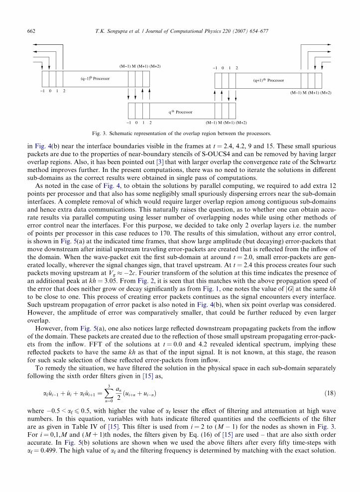
Fig. 3. Schematic representation of the overlap region between the processors.
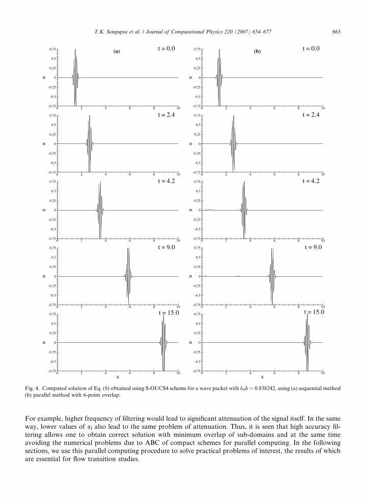
662 T.K. Sengupta et al. / Journal of Computational Physics 220 (2007) 654–677
in Fig. 4(b) near the interface boundaries visible in the frames at t = 2.4, 4.2, 9 and 15. These small spuriouspackets are due to the properties of near-boundary stencils of S-OUCS4 and can be removed by having largeroverlap regions. Also, it has been pointed out [3] that with larger overlap the convergence rate of the Schwartzmethod improves further. In the present computations, there was no need to iterate the solutions in differentsub-domains as the correct results were obtained in single pass of computations.
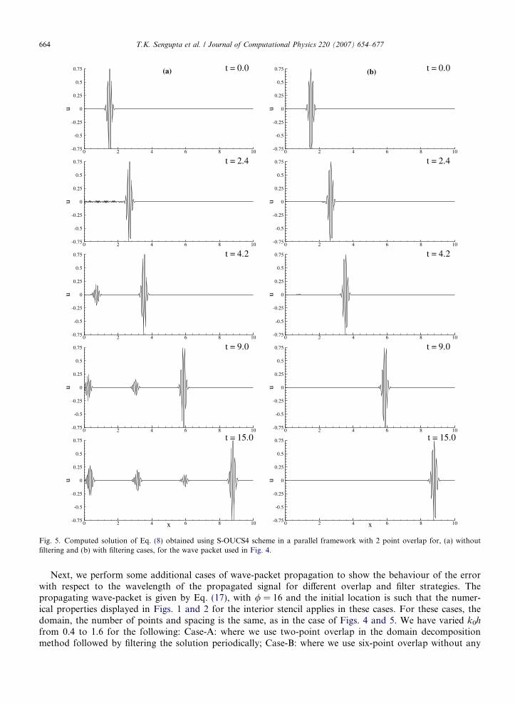
As noted in the case of Fig. 4, to obtain the solutions by parallel computing, we required to add extra 12points per processor and that also has some negligibly small spuriously dispersing errors near the sub-domaininterfaces. A complete removal of which would require larger overlap region among contiguous sub-domainsand hence extra data communications. This naturally raises the question, as to whether one can obtain accu-rate results via parallel computing using lesser number of overlapping nodes while using other methods oferror control near the interfaces. For this purpose, we decided to take only 2 overlap layers i.e. the numberof points per processor in this case reduces to 170. The results of this simulation, without any error control,is shown in Fig. 5(a) at the indicated time frames, that show large amplitude (but decaying) error-packets thatmove downstream after initial upstream traveling error-packets are created that is reflected from the inflow ofthe domain. When the wave-packet exit the first sub-domain at around t = 2.0, small error-packets are gen-erated locally, wherever the signal changes sign, that travel upstream. At t = 2.4 this process creates four suchpackets moving upstream at Vg � �2c. Fourier transform of the solution at this time indicates the presence ofan additional peak at kh = 3.05. From Fig. 2, it is seen that this matches with the above propagation speed ofthe error that does neither grow or decay significantly as from Fig. 1, one notes the value of jGj at the same kh
to be close to one. This process of creating error packets continues as the signal encounters every interface.Such upstream propagation of error packet is also noted in Fig. 4(b), when six point overlap was considered.However, the amplitude of error was comparatively smaller, that could be further reduced by even largeroverlap.
However, from Fig. 5(a), one also notices large reflected downstream propagating packets from the inflowof the domain. These packets are created due to the reflection of those small upstream propagating error-pack-ets from the inflow. FFT of the solutions at t = 0.0 and 4.2 revealed identical spectrum, implying thesereflected packets to have the same kh as that of the input signal. It is not known, at this stage, the reasonfor such scale selection of these reflected error-packets from inflow.
To remedy the situation, we have filtered the solution in the physical space in each sub-domain separatelyfollowing the sixth order filters given in [15] as,
af ui�1 þ ui þ af uiþ1 ¼X3
n¼0
an
2ðuiþn þ ui�nÞ ð18Þ
where �0.5 < af 6 0.5, with higher the value of af lesser the effect of filtering and attenuation at high wavenumbers. In this equation, variables with hats indicate filtered quantities and the coefficients of the filterare as given in Table IV of [15]. This filter is used from i = 2 to (M � 1) for the nodes as shown in Fig. 3.For i = 0,1,M and (M + 1)th nodes, the filters given by Eq. (16) of [15] are used – that are also sixth orderaccurate. In Fig. 5(b) solutions are shown when we used the above filters after every fifty time-steps withaf = 0.499. The high value of af and the filtering frequency is determined by matching with the exact solution.
u
0 2 4 6 8 10-0.75
-0.5
-0.25
0
0.25
0.5
0.75 t = 0.0(b)
u
0 2 4 6 8 10-0.75
-0.5
-0.25
0
0.25
0.5
0.75 t = 2.4
u
0 2 4 6 8 10-0.75
-0.5
-0.25
0
0.25
0.5
0.75 t = 4.2
x
u
0 2 4 6 8 10-0.75
-0.5
-0.25
0
0.25
0.5
0.75 t = 15.0
u
0 2 4 6 8 10-0.75
-0.5
-0.25
0
0.25
0.5
0.75 t = 2.4
u
0 2 4 6 8 10-0.75
-0.5
-0.25
0
0.25
0.5
0.75 t = 4.2
u
0 2 4 6 8 10-0.75
-0.5
-0.25
0
0.25
0.5
0.75 t = 9.0
x
u
0 2 4 6 8 10-0.75
-0.5
-0.25
0
0.25
0.5
0.75 t = 15.0
u
0 2 4 6 8 10-0.75
-0.5
-0.25
0
0.25
0.5
0.75 t = 9.0
u
0 2 4 6 8 10-0.75
-0.5
-0.25
0
0.25
0.5
0.75 t = 0.0(a)
Fig. 4. Computed solution of Eq. (8) obtained using S-OUCS4 scheme for a wave packet with k0h = 0.838242, using (a) sequential method(b) parallel method with 6-point overlap.
T.K. Sengupta et al. / Journal of Computational Physics 220 (2007) 654–677 663
For example, higher frequency of filtering would lead to significant attenuation of the signal itself. In the sameway, lower values of af also lead to the same problem of attenuation. Thus, it is seen that high accuracy fil-tering allows one to obtain correct solution with minimum overlap of sub-domains and at the same timeavoiding the numerical problems due to ABC of compact schemes for parallel computing. In the followingsections, we use this parallel computing procedure to solve practical problems of interest, the results of whichare essential for flow transition studies.
u
0 2 4 6 8 10-0.75
-0.5
-0.25
0
0.25
0.5
0.75 t = 0.0(a)u
0 2 4 6 8 10-0.75
-0.5
-0.25
0
0.25
0.5
0.75 t = 2.4
u
0 2 4 6 8 10-0.75
-0.5
-0.25
0
0.25
0.5
0.75 t = 4.2
u
0 2 4 6 8 10-0.75
-0.5
-0.25
0
0.25
0.5
0.75 t = 9.0
u
0 2 4 6 8 10-0.75
-0.5
-0.25
0
0.25
0.5
0.75 t = 9.0
u
0 2 4 6 8 10-0.75
-0.5
-0.25
0
0.25
0.5
0.75 t = 4.2
x
u
0 2 4 6 8 10-0.75
-0.5
-0.25
0
0.25
0.5
0.75 t = 15.0
x
u
0 2 4 6 8 10-0.75
-0.5
-0.25
0
0.25
0.5
0.75 t = 15.0
u
0 2 4 6 8 10-0.75
-0.5
-0.25
0
0.25
0.5
0.75 t = 0.0(b)
u
0 2 4 6 8 10-0.75
-0.5
-0.25
0
0.25
0.5
0.75 t = 2.4
Fig. 5. Computed solution of Eq. (8) obtained using S-OUCS4 scheme in a parallel framework with 2 point overlap for, (a) withoutfiltering and (b) with filtering cases, for the wave packet used in Fig. 4.
664 T.K. Sengupta et al. / Journal of Computational Physics 220 (2007) 654–677
Next, we perform some additional cases of wave-packet propagation to show the behaviour of the errorwith respect to the wavelength of the propagated signal for different overlap and filter strategies. Thepropagating wave-packet is given by Eq. (17), with / = 16 and the initial location is such that the numer-ical properties displayed in Figs. 1 and 2 for the interior stencil applies in these cases. For these cases, thedomain, the number of points and spacing is the same, as in the case of Figs. 4 and 5. We have varied k0h
from 0.4 to 1.6 for the following: Case-A: where we use two-point overlap in the domain decompositionmethod followed by filtering the solution periodically; Case-B: where we use six-point overlap without any

T.K. Sengupta et al. / Journal of Computational Physics 220 (2007) 654–677 665
filtering and Case-C: where the solution is obtained using six-point overlapped domains followed by peri-odic filtering.
The error in all these cases is calculated from, L1ðErrorÞ ¼PM
i¼1jðuiÞexact � ðuiÞcomputedj=M . We note that theerror is caused primarily by: (i) attenuation of the actual signal; and (ii) by the dispersion of the computedsignal. For the former source of error, the magnitude can be at most equal to the area under the wave-packet,in the absence of phase error. While the maximum error that can be created by dispersion alone- in the absenceof attenuation – is equal to twice the area created under the wave packet. Therefore, in the presence of dis-persion and dissipation, the maximum error can at most be equal to twice the area under the curve.
In Fig. 6(a), L1(Error) is plotted for the above-mentioned cases for different values of k0h, that shows theerror to be of same order of magnitude, up to k0h @ 1. For k0h = 1.2, it is noted that Case-A has the least error.Case-B, like Case-A produces reflection at the domain interface that travels upstream and is left uncontrolledthat causes this case to have largest error in Fig. 6(a), for all k0h except for 1.4. This reflection of Case-B is
k0 h
(VgN
/c-1
)
0.4 0.6 0.8 1 1.2 1.4 1.6
-0.03
-0.02
-0.01
0
0.01
0.02
0.03
P
(b)
x
u
8.2 8.4 8.6 8.8 9 9.2 9.4 9.6
-0.8
-0.6
-0.4
-0.2
0
0.2
0.4
0.6
0.8
1 Exact solutionCase-ACase-C
(c)
k0 h
L∞
(err
or)
0.4 0.6 0.8 1 1.2 1.4 1.6
0.015
0.02
0.025
0.03
0.035
0.04
0.045
0.05
2-overlap with filtering (Case-A)6-overlap (Case-B)6-overlap with filtering (Case-C)
(a)
Fig. 6. (a) L1 norm of the error with respect to the exact solution is plotted against k0h for the indicated cases. (b) Departure of the scalednumerical group velocity from unity (dispersion error) is shown for different values of k0h. (c) Computed solution of Eq. (8) has beencompared with the exact solution for a wave packet with k0h = 1.2.
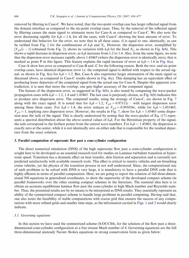
666 T.K. Sengupta et al. / Journal of Computational Physics 220 (2007) 654–677
removed by filtering in Case-C. We have noted, that the two-point overlap case has larger reflected signal fromthe domain interface as compared to the six-point overlap cases. Thus, by the removal of the reflected signalby filtering causes the main signal to attenuate more for Case-A as compared to Case-C. We also note theerror decreasing rapidly for k0h = 1.4, for all the cases, with Case-C showing the least amount of error. Tounderstand this behavior for the error, we note that in all these cases, G is equal to one, identically, as canbe verified from Fig. 1 for the combinations of k0h and Nc. However, the dispersion error, exemplified by[VgN/c � 1] (obtained from Fig. 2), shows its variation with k0h for the fixed Nc, as shown in Fig. 6(b). Thisshows a rapid decrease in dispersion error, as k0h increases from 1.2 to 1.4. Also, from the same figure, we notethat the dispersion error increases rapidly above 1.45465 (where the dispersion error is identically zero), that ismarked as point P in this figure. This feature explains the rapid increase of error at k0h = 1.6 in Fig. 6(a).
Case-A show less error as compared to Case-B and -C for the following reason. Both the two- and six-pointoverlap cases, have identical dispersion error i.e. the computed signal is shifted with respect to the actual sig-nal- as shown in Fig. 6(c) for k0h = 1.2. But, Case-A also experience larger attenuation of the main signal asdiscussed above, as compared to Case-C results shown in Fig. 6(c). This damping has an equivalent effect ofproducing lesser departure of the computed signal from the actual one for Case-A. Despite this apparent con-tradiction, it is seen that more the overlap, one gets higher accuracy of the computed signal.
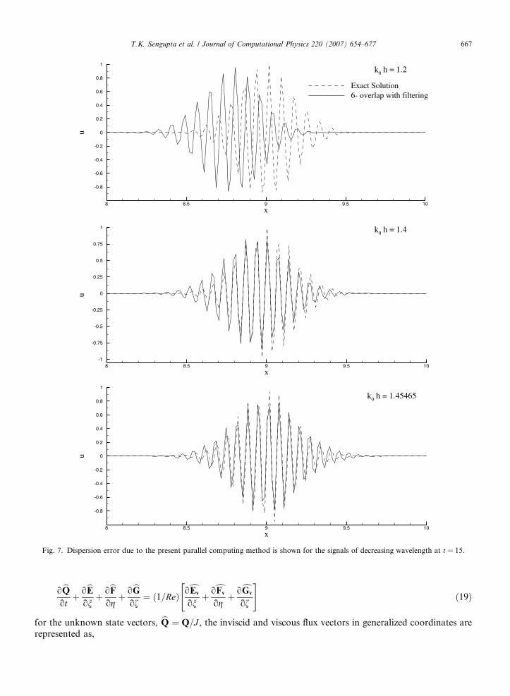
The feature of the dispersion error, as suggested in Fig. 6(b), is also tested by computing the wave-packetpropagation cases with k0h = 1.2, 1.4 and 1.45465. The last case is purposely chosen, as Fig. 6(b) indicates thisto produce zero dispersion error. The computed results, using the strategy of Case-C, are shown in Fig. 7along with the exact signal. It is noted that for k0h = 1.2, VgN = 0.97112c – with largest dispersion erroramong these three cases. For k0h = 1.4, the error reduces as VgN = 0.991034c, while for k0h = 1.451465,VgN = 1, implying zero dispersion error. However, the results in Fig. 7, show for k0h = 1.45465 some disper-sion near the tails of the signal. This is clearly understood by noting that the wave-packet of Eq. (17) repre-sents a spectral distribution about the above central values of k0h. For the Hermitian property of the signal,the tails correspond to the farthest points from the central wave numbers. For k0h = 1.45465, the dispersion isexactly zero at the center, while it is not identically zero on either side that is responsible for the residual depar-ture from the exact solution.
3. Parallel computation of supersonic flow past a cone-cylinder configuration
The direct numerical simulation (DNS) of the high supersonic flow past a cone-cylinder configuration issought here to be developed as an essential research tool for studies on Laminar-turbulent transition at hyper-sonic speed. Transition has a dramatic effect on heat transfer, skin friction and separation and is currently notpredicted satisfactorily with available research tools. This effect is critical to reentry vehicles and air-breathingcruise vehicles, yet the physics of the transition process in not well understood. Since, the computational sizeof such problems to be solved with DNS is very large, it is mandatory to have a parallel DNS code that ishighly efficient in terms of parallel computation. Here, we are going to report the solution of full three-dimen-sional NS equations in generalized coordinates, to show the superiority of the developed compact scheme (inparallel framework) over the other existing compact schemes in the literature. The essential idea here is toobtain an accurate equilibrium laminar flow past the cone-cylinder at high Mach number and Reynolds num-ber. Thus, the presented results are by no means to be interpreted as DNS results. They essentially represent anability of the symmetrized compact scheme to handle large problems in parallel computing. Having said that,one also notes the feasibility of stable computations with coarse grid that ensures the success of any compu-tations with more refined grids and smaller time steps, as the information carried in Figs. 1 and 2 would clearlyindicate.
3.1. Governing equations
In this section we have used the symmetrized scheme (S-OUCS4), for the solution of the flow past a three-dimensional cone-cylinder configuration at a free stream Mach number of 4. Governing equations are the fullthree-dimensional unsteady Navier–Stokes equations in strong conservation form as given below:
x
u
8 8.5 9 9.5 10-1
-0.75
-0.5
-0.25
0
0.25
0.5
0.75
1 k0 h = 1.4
x
u
8 8.5 9 9.5 10
-0.8
-0.6
-0.4
-0.2
0
0.2
0.4
0.6
0.8
1
k0 h = 1.45465
x
u
8 8.5 9 9.5 10
-0.8
-0.6
-0.4
-0.2
0
0.2
0.4
0.6
0.8
1
Exact Solution6- overlap with filtering
k0 h = 1.2
Fig. 7. Dispersion error due to the present parallel computing method is shown for the signals of decreasing wavelength at t = 15.
T.K. Sengupta et al. / Journal of Computational Physics 220 (2007) 654–677 667
o bQotþ obE
onþ obF
ogþ obG
of¼ ð1=ReÞ ocEv
onþ ocFv
ogþ ocGv
of
" #ð19Þ
for the unknown state vectors, bQ ¼ Q=J , the inviscid and viscous flux vectors in generalized coordinates arerepresented as,
668 T.K. Sengupta et al. / Journal of Computational Physics 220 (2007) 654–677
bE ¼ ð1=JÞðnxEþ nyFþ nzGÞbF ¼ ð1=JÞðgxEþ gyFþ gzGÞbG ¼ ð1=JÞðfxEþ fyFþ fzGÞcEv ¼ ð1=JÞðnxEv þ nyFv þ nzGvÞcFv ¼ ð1=JÞðgxEv þ gyFv þ gzGvÞcGv ¼ ð1=JÞðfxEv þ fyFv þ fzGvÞ
whereQ ¼ ½q; qu; qv; qw; qe�T
E ¼ ½qu; qu2 þ p; qvu; qwu; ðqeþ pÞu�T
F ¼ ½qv; quv; qv2 þ p; qwv; ðqeþ pÞv�T
G ¼ ½qw; quw; qvw; qw2 þ p; ðqeþ pÞw�T
Ev ¼ ½0; sxx; sxy ; sxz; usxx þ vsxy þ wsxz þ qx�T
Fv ¼ ½0; syx; syy ; syz; usyx þ vsyy þ wsyz þ qy �T
Gv ¼ ½0; szx; szy ; szz; uszx þ vszy þ wszz þ qz�T
The various stress tensor components (sij) and the heat flux components (qi) can be further written as:
sxx ¼ 2louoxþ kr:V
� �syy ¼ 2l
ouoyþ kr:V
� �szz ¼ 2l
ouozþ kr:V
� �sxy ¼ syx ¼ l
ouoyþ ov
ox
� �syz ¼ szy ¼ l
ovozþ ow
oy
� �szx ¼ sxz ¼ l
owoxþ ou
oz
� �qx ¼
l
ðc� 1ÞPrM21
oTox
qy ¼l
ðc� 1ÞPrM21
oToy
qz ¼l
ðc� 1ÞPrM 21
oToz
In the expressions above, u, v, w are the Cartesian velocity components, q is the density, p is the pressure and e
is the total energy per unit mass defined as, e = p/[(c � 1)q] + (u2 + v2 + w2)/2. The perfect gas relationshipp ¼ qT=ðcM2
1Þ is also assumed; c = cp/cv is the ratio of specific heats and is taken as 1.4 in the present case.Here, l is the dynamic viscosity and k from the Stokes’ hypothesis is �2l/3. The Jacobian of grid transfor-mation is represented as J in the expressions above. All the flow variables have been normalized by theirrespective free stream values except for pressure, which has been non-dimensionalized by q1c2
1. Reynoldsnumber is indicated as Re in Eq. (19), which is equal to 1.12 · 106 for the present problem, based on c1and the cylinder diameter (D). Also, Pr is the Prandtl number in the above expressions and is equal to 0.7in the present computation.
T.K. Sengupta et al. / Journal of Computational Physics 220 (2007) 654–677 669
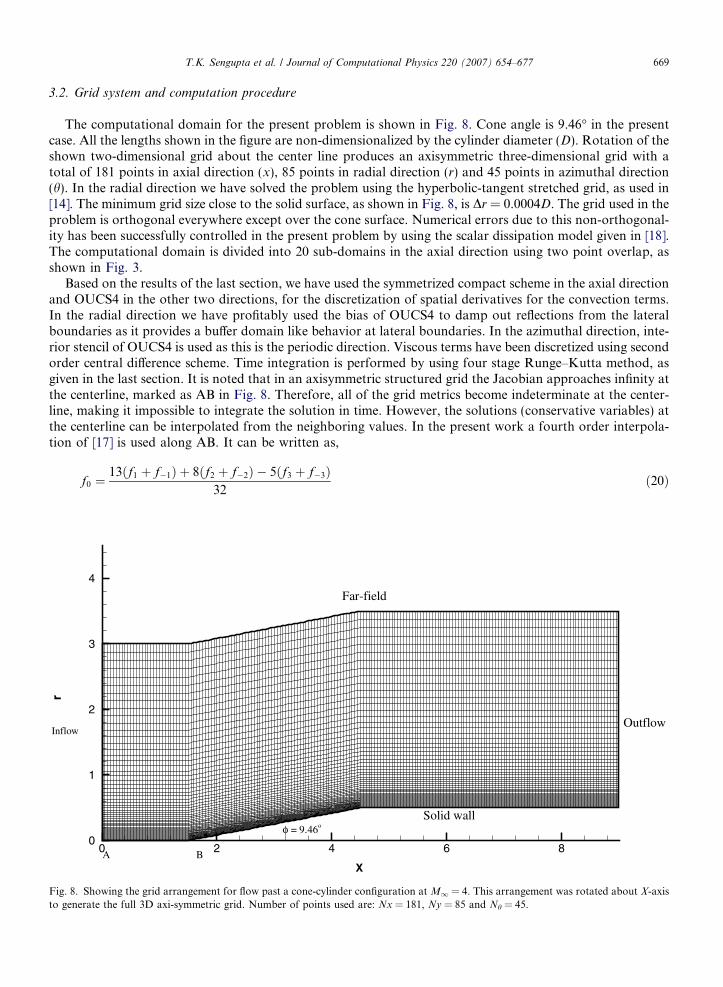
3.2. Grid system and computation procedure
The computational domain for the present problem is shown in Fig. 8. Cone angle is 9.46� in the presentcase. All the lengths shown in the figure are non-dimensionalized by the cylinder diameter (D). Rotation of theshown two-dimensional grid about the center line produces an axisymmetric three-dimensional grid with atotal of 181 points in axial direction (x), 85 points in radial direction (r) and 45 points in azimuthal direction(h). In the radial direction we have solved the problem using the hyperbolic-tangent stretched grid, as used in[14]. The minimum grid size close to the solid surface, as shown in Fig. 8, is Dr = 0.0004D. The grid used in theproblem is orthogonal everywhere except over the cone surface. Numerical errors due to this non-orthogonal-ity has been successfully controlled in the present problem by using the scalar dissipation model given in [18].The computational domain is divided into 20 sub-domains in the axial direction using two point overlap, asshown in Fig. 3.
Based on the results of the last section, we have used the symmetrized compact scheme in the axial directionand OUCS4 in the other two directions, for the discretization of spatial derivatives for the convection terms.In the radial direction we have profitably used the bias of OUCS4 to damp out reflections from the lateralboundaries as it provides a buffer domain like behavior at lateral boundaries. In the azimuthal direction, inte-rior stencil of OUCS4 is used as this is the periodic direction. Viscous terms have been discretized using secondorder central difference scheme. Time integration is performed by using four stage Runge–Kutta method, asgiven in the last section. It is noted that in an axisymmetric structured grid the Jacobian approaches infinity atthe centerline, marked as AB in Fig. 8. Therefore, all of the grid metrics become indeterminate at the center-line, making it impossible to integrate the solution in time. However, the solutions (conservative variables) atthe centerline can be interpolated from the neighboring values. In the present work a fourth order interpola-tion of [17] is used along AB. It can be written as,
r
Inflow
Fig. 8.to gen
f0 ¼13ðf1 þ f�1Þ þ 8ðf2 þ f�2Þ � 5ðf3 þ f�3Þ
32ð20Þ
X
0 2 4 6 80
1
2
3
4
Outflow
Far-field
Solid wall
A B
φ = 9.46o
Showing the grid arrangement for flow past a cone-cylinder configuration at M1 = 4. This arrangement was rotated about X-axiserate the full 3D axi-symmetric grid. Number of points used are: Nx = 181, Ny = 85 and Nh = 45.
670 T.K. Sengupta et al. / Journal of Computational Physics 220 (2007) 654–677
where the negative indices mean the values in the opposite direction across the centerline. This results in asmany sets of interpolated values as half the number of grid points in the azimuthal direction. A unique valueof the centerline solution is finally obtained by averaging these values.
High accuracy schemes in space and time resolve a wider range of wave number or frequency, as notedfrom Figs. 1 and 2. However, there are still some high wavenumber/frequencies which gives rise to spu-rious numerical oscillations due to dispersion – note the VgN/c for kh > 2.4 in Fig. 2 for all interior nodes.This is true specially in a region where grid is non-orthogonal. To avoid such numerical errors from con-taminating the result, a scalar dissipation model of [18] is used in the present computation, takinga2 = 0.25 and a4 = 1/64. This will also help us in getting rid of spurious reflections from the interfaceboundaries, as we experienced in the last section with the propagation of wave-packet. This artificial dis-sipation model is implemented only at the last stage of the Runge–Kutta time integration scheme in orderto minimize the computational costs.
In addition to the reflection from the interfacial boundaries, there might be some reflection from the geo-metrical boundaries. Such reflection from the inflow was observed in Fig. 5(a), where the reflected wave hadamplitude much higher than the incident one. Therefore, in addition to the requirement of these high accuracyschemes and artificial numerical dissipation, one must have a non-reflecting boundary condition to allowsmooth passage to the incoming waves. To meet this requirement, generalized characteristic boundary condi-tion of [16] is used in the present computation, for conditions at the solid wall. Free stream values have beenused at all other boundaries of the computational domain, except at the outflow, where simple second orderextrapolation [19] is used to generate a non-reflecting condition. Such simple conditions at all other bound-aries are possible because of high free stream Mach number (M1 = 4) of the present problem. For M1 > 1the characteristic convection speed of all the waves is unidirectional, i.e in the direction of the mean flow,whereas for M1 < 1, one is forced to use characteristic boundary condition at the inflow/outflow, in orderto achieve a reflection-free condition. In the azimuthal direction periodic boundary condition is used for thisaxisymmetric geometry.
3.3. Results and discussion
Starting with a uniform flow condition everywhere, Eq. (19) is integrated in time following the computationprocedure discussed in the previous subsection. The time step for the present computation is small(Dt = 3 · 10�5) so as to maintain a near-neutral behavior of the numerical schemes for long time integration[14]. The Mach number contours, hence obtained are shown in Fig. 9(a), at the indicated times. Contours areshown in the (r–x)-plane for h = p/2. No reflection is observed either at the interfacial boundaries or the out-flow/inflow boundaries – as this is effectively controlled by selective addition of second and fourth order dis-sipation [18]. One notes the formation of an oblique shock at the vertex of the cone and an expansion fan atthe cone-cylinder junction. Cross-sectional view of the contours are plotted in Fig. 9(b), at x/D = 4.45, markedby dotted lines in Fig. 9(a). One notes a perfectly symmetrical result at these cross-sections and no visiblechange in the contours, with time but there are changes in the contours very close to the surface that havenot been plotted here.
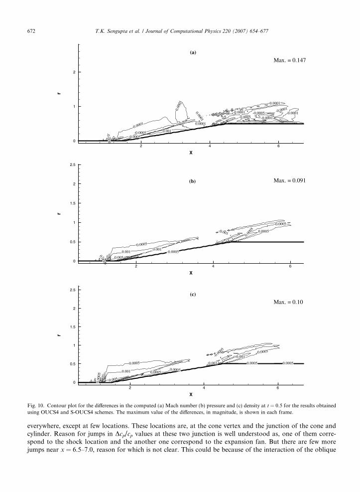
To show the superiority of the symmetrized compact scheme (S-OUCS4) over the OUCS4 scheme in theaxial direction, another case is run using OUCS4 in the axial direction as well, using two point overlap atthe interface boundaries. Results obtained are very revealing in showing the difference between these two setsof calculations as shown in Fig. 10. In Fig. 10(a), difference in Mach number contours obtained by S-OUCS4and OUCS4 schemes is shown at t = 0.5. Significant differences are noted near the cone vertex and the cone-cylinder junction. The magnitude of maximum difference is noted in all the frames of Fig. 10 for differentquantities. The values differ in first decimal place, very close to the surface and keeps on reducing as we moveup in radial direction, as one would expect from such high Mach number flow. Similar trends are seen inFig. 10(b) and (c), where difference in pressure and density contours are shown at the same time. It is to benoted that same code is used for the two cases, just that S-OUCS4 is replaced by OUCS4 in the latter in axialdirection. This leads us to conclude that these differences are only due to the near-boundary behavior ofOUCS4, which develops a directional bias in the derivatives, causing more reflection from the interfacialboundaries. One can note this directionality of OUCS4 from the jGj and VgN/c contours shown in Figs. 1

YZ
-0.5 0 0.5 1
-0.5
0
0.5
t = 2
Y
Z
-0.5 0 0.5 1
-0.5
0
0.5
t = 3
Y
Z
-0.5 0 0.5 1
-0.5
0
0.5
t = 8
X
r
0 2 4 6 80
1
2
3
4
X
r
0 2 4 6 80
1
2
3
4
X
r
0 2 4 6 80
1
2
3
4
X
r
0 2 4 6 80
1
2
3
4
(a)
Y
Z
-0.5 0 0.5 1
-0.5
0
0.5
t = 1
(b)
Fig. 9. Mach number contours, at the indicated times, are shown for a supersonic flow (M1 = 4) past a cone-cylinder configuration usingS-OUCS4 with 2 points overlap, (a) for h = 90� location, (b) the cross-sectional view at the dotted location of figure (a).
T.K. Sengupta et al. / Journal of Computational Physics 220 (2007) 654–677 671
and 2. From the same figures, one can note the improvement in stability characteristics of S-OUCS4 overOUCS4, specially at the near boundary nodes. It is very difficult to make out near wall behavior from the con-tour plots of Fig. 10. For this reason, relative change in coefficient of pressure (Dcp/cp) between these two setsof calculations, is plotted in Fig. 11, for j = 1–3, with j = 1 identifying the wall itself. It is noted that differencesare as high as 2.0, which can certainly affect calculations based on these cp values. These differences are small
0.00
01
-0.0001 0.0001
0.001-0.0005-0.0005
0.0001
0.0001
-0.0005-0.0001 -0.0001
-0.0001-0.00050.0001
-0.000
X
r
2 4 60
1
2
(a)
Max. = 0.147
0.0005
0.001
0.00050.005
0.001-0.0005
-0.001
0.0005
0.0005
0.00
05
X
r
2 4 60
0.5
1
1.5
2
2.5
(b) Max. = 0.091
0.0005
0.001
0.00
05
0.0005
0.005
-0.0005
0.00050.001
0.001 0.0005
0.0005
0.0005
X
r
2 4 60
0.5
1
1.5
2
2.5(c)
Max. = 0.10
Fig. 10. Contour plot for the differences in the computed (a) Mach number (b) pressure and (c) density at t = 0.5 for the results obtainedusing OUCS4 and S-OUCS4 schemes. The maximum value of the differences, in magnitude, is shown in each frame.
672 T.K. Sengupta et al. / Journal of Computational Physics 220 (2007) 654–677
everywhere, except at few locations. These locations are, at the cone vertex and the junction of the cone andcylinder. Reason for jumps in Dcp/cp values at these two junction is well understood as, one of them corre-spond to the shock location and the another one correspond to the expansion fan. But there are few morejumps near x = 6.5–7.0, reason for which is not clear. This could be because of the interaction of the oblique
X
Δcp/c
p
0 2 4 6 8
0
0.5
1
1.5
2
j = 1
X
Δcp/c
p
0 2 4 6 8
-5
0
5
10
15
20
25
30
35
j = 2
X
Δcp/c
p
0 2 4 6 8-1.5
-1
-0.5
0
0.5
1
1.5
2
2.5
3
j = 3
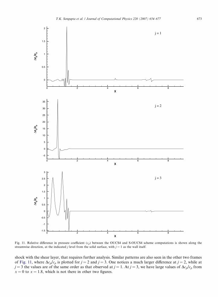
Fig. 11. Relative difference in pressure coefficient (cp) between the OUCS4 and S-OUCS4 scheme computations is shown along thestreamwise direction, at the indicated j level from the solid surface, with j = 1 as the wall itself.
T.K. Sengupta et al. / Journal of Computational Physics 220 (2007) 654–677 673
shock with the shear layer, that requires further analysis. Similar patterns are also seen in the other two framesof Fig. 11, where Dcp/cp is plotted for j = 2 and j = 3. One notices a much larger difference at j = 2, while atj = 3 the values are of the same order as that observed at j = 1. At j = 3, we have large values of Dcp/cp fromx = 0 to x = 1.8, which is not there in other two figures.
674 T.K. Sengupta et al. / Journal of Computational Physics 220 (2007) 654–677
Overall, the calculated results using S-OUCS4 scheme are seen to be adequate in capturing the equilibriumlaminar flow, whose receptivity to imposed acoustic, vortical and entropic disturbances will be studied infuture.
4. Convection of a shielded vortex in subsonic flows
Finally, the case for the convection of a shielded vortex is studied at low subsonic speed to check whetherthe present method of domain decomposition extends to elliptic cases or not. This allows us to estimate theerror committed in the multiprocessor computing with respect the serial calculation of the same. In a shieldedvortex, the core is surrounded by an annular ring with vorticity of opposite sign. The shielded vortex studiedhere correspond to the two-parameter inviscid distributed vortex given by,
Y
6
8
10
12
14
16
Y
6
8
10
12
14
16
Y
6
8
10
12
14
16
Fig. 12(c) 6 n
x ¼ Kð1� a1r2Þe�a2r2 ð21Þ
This vortex can have non-zero circulation, depending upon the values of a1 and a2, as given by,C ¼ pKa2
ð1� a1=a2Þ ð22Þ
X
10 15 20
X
Y
10 15 20
6
8
10
12
14
16
X
10 15 20
X
Y
10 15 20
6
8
10
12
14
16
X
10 15 20
(a) np = 1
X
Y
10 15 20
6
8
10
12
14
16
(b) np = 3
X
Y
10 15 20
6
8
10
12
14
16
t = 30
X
Y
10 15 20
6
8
10
12
14
16
t = 20
X
Y
10 15 20
6
8
10
12
14
16
t = 10
(c) np = 6
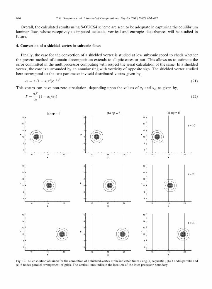
. Euler solution obtained for the convection of a shielded-vortex at the indicated times using (a) sequential; (b) 3 nodes parallel andodes parallel arrangement of grids. The vertical lines indicate the location of the inter-processor boundary.
T.K. Sengupta et al. / Journal of Computational Physics 220 (2007) 654–677 675
In the present work, we have used a1 = a2 = 1/2, that gives rise to a vortex with zero circulation and that cre-ates the velocity and pressure distribution given in Section 4.1.1. of Ref. [15]. The vortex of Eq. (21) also ischaracterized by the presence of an inflexion point for the velocity distribution i.e. ox
or ¼ 0. It is well knownthat such velocity profiles are very susceptible to inviscid instabilities – as given in [20] as a necessary conditionfor the centrifugal instability for two-dimensional non-axisymmetric disturbances. This instability is physicalin nature, as it was studied in [21] where the mono-polar vortex gave rise to a tripolar structure upon the appli-cation of small amplitude disturbances, that could also be triggered by numerical error.
In the following, we have performed calculations for a case, where a vortex of non-dimensional strengthequal to 0.02 convects in a free stream at the Mach number M1 = 0.4. Subsonic cases are more sensitiveto the boundary closures than the supersonic case because for M1 < 1 the flow is elliptic in nature and thewaves are not unidirectional, as in the case of M1 > 1. For this reason, the flow in this case is more susceptible
number of processors
elap
sed
time
(sec
onds
)
1 2 3 4 5 6
750
1000
1250
1500
1750
2000
(b)
t
erro
r
10 20 30
5E-08
1E-07
1.5E-07
2E-07
number of processors = 3number of processors = 6
(a)
Fig. 13. (a) Time variation of the L2 norm of the error due to parallel computing using the present domain decomposition technique isshown for the test case of Section 4. (b) Shows the efficiency of the present parallel computing method with respect to the elapsed time (inseconds) and number of processors.
676 T.K. Sengupta et al. / Journal of Computational Physics 220 (2007) 654–677
to reflection at the interface boundaries. The computational domain for the present case varies from0 6 x 6 30 and 0 6 y 6 20 with 301 points in the x direction and 201 points in the y direction such thatDx = Dy = 0.1. At t = 0, the vortex is centered at x = 7.5 and the computation is carried out till the non-dimensional time of t = 30. It is to be noted that the velocity scale for this problem is the speed of soundand hence the non-dimensional convection speed of the vortex is U1 = 0.4. In this section, we have usedthe symmetrized scheme (S-OUCS3) developed in [14] to show the identical beneficial effects of symmetriza-tion of any compact scheme. Also, explicit fourth order numerical dissipation is used to suppress high fre-quency reflection from the inter-domain boundaries. Slight use of numerical damping is necessary to seethe best performance of the symmetrized compact schemes using the present parallel computing method, asthere will always be some high frequency non-zero reflections from the inter-domain boundaries, that whenleft uncontrolled, can contaminate the solution everywhere [22]. Time dependent characteristics based bound-ary conditions are used on density, at all the geometrical boundaries to avoid reflection from them.
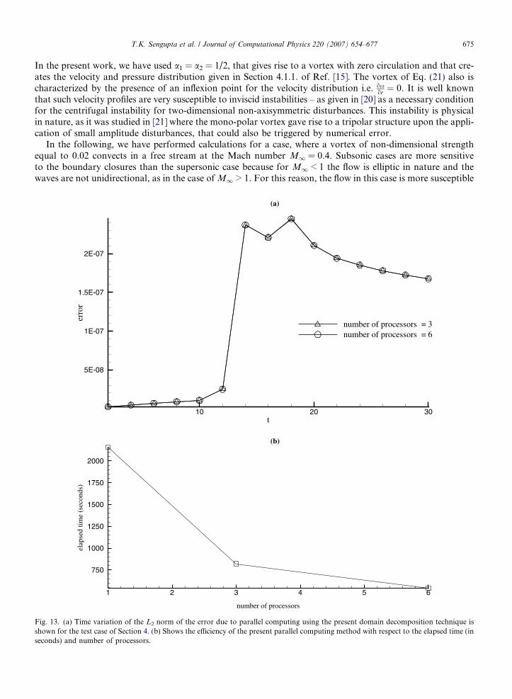
Three different cases have been performed using 1, 3 and 6 processors splitting the problem in the stream-wise (x) direction with six-point overlap strategy. The number of grid points are divided equally among theprocessors to make a perfect load balance. The first case with single processor, corresponds to serial comput-ing and is undertaken to measure the error of parallel computing with respect to this serial benchmark. Theresults in Fig. 12, show the vorticity contours at different time instants for the three cases. The vertical lines inthese figures, indicate the locations of the inter-domain/inter-processor boundaries. Comparison of Figs. 12(b)and (c) with Fig. 12(a) clearly shows that the results of parallel computations match perfectly with the sequen-tial results and the error induced by reflections from the inter-domain boundaries are negligible and can not beobserved visually. A quantitative measure of the error (usequential � uparallel), in parallel computation frame-work, is shown by the time variation of the L2 norm of the error in Fig. 13(a). The errors are negligibly small,of the order of 10�7. It is also noted that the error remains the same when the number of processors increases.
In Fig. 13(b), elapsed time (in seconds) of these cases are plotted against the number of processors in orderto show the parallel efficiency of the present method. The figure shows that the parallel efficiency keeps comingdown with increase in number of processors. This is due to the larger number of information transfer acrossthe inter-domain boundaries, associated with six-point overlap method used in this test case.
5. Summary
Compact schemes have been specifically designed for parallel computing using domain decompositionmethod. While retaining the excellent numerical properties of compact schemes for DNS, the streamwise biasof these schemes have been reduced significantly by symmetrization so that the resultant scheme can be usedfor parallel domain decomposition methods with minimal overlap. The remaining problems of parallel com-puting using compact schemes are removed by adopting any one of the following: (a) larger overlap of sub-domains, with and without filtering [15] of the solution; (b) reducing the overlap, with mandatory filtering ofthe solution in sub-domains and (c) selective addition of artificial second and fourth order dissipation [18]. Thedeveloped procedures for (a) and (b) have been calibrated for the propagation of a wave-packet following lin-ear convection equation. We have performed detailed error analysis identifying the contributing sources andshowing that the six-point overlap is more accurate than the two-point overlap domain-decompositionmethod. Procedures adopted for (c) has been shown by solving 3D unsteady Navier–Stokes equations forRe = 1.12 · 106, M1 = 4 flow past a cone-cylinder.
References
[1] A. Quarteroni, A. Valli, Domain Decomposition Methods for Partial Differential Equations, Oxford University Press, Oxford, UK,1999.
[2] B.F. Smith, P. Bjorstad, W. Gropp, Domain Decomposition, Parallel Multilevel Methods for Elliptic Partial Differential Equations,Cambridge University Press, New York, 1996.
[3] V. Dolean, S. Lanteri, F.C. Nataf, Int. J. Num. Meth. Fluids 40 (2002) 1539.[4] P.L. Lions, in: T.F. Chan, R. Glowinski, J. Periaux, O. Widlund (Eds.), Third International Symposium on Domain Decomposition
Methods for Partial Differential Equations, SIAM, Philadelphia, PA, 1990.[5] J.S. Shang, J.A. Camberos, M.D. White, Advances in time-domain computational electromagnetics, AIAA Paper no., 99-3731, 1999..
T.K. Sengupta et al. / Journal of Computational Physics 220 (2007) 654–677 677
[6] D.P. Lockard, P.J. Morris, J. Comput. Acoust. 5 (1997) 337.[7] A. Povitsky, P.J. Morris, ICASE Report No. 99-34, 1999.[8] S.K. Lele, J. Comput. Phys. 103 (1992) 16.[9] T.K. Sengupta, G. Ganeriwal, S. De, J. Comput. Phys. 192 (2) (2003) 677.
[10] T.K. Sengupta, S.K. Sircar, A. Dipankar, J. Sci. Comput. 26 (2) (2006) 151.[11] J.J. Dongarra, I.S. Duff, D.C. Sorenson, H.A. Van der Vorst, Numerical Linear Algebra for High Performance Computers, SIAM,
Philadelphia, 1998.[12] J. Hofhaus, E.F. Van de Velde, SIAM J. Sci. Comput. 17 (2) (1996) 454.[13] X.-H. Sun, Parallel Comput. 21 (8) (1995) 1241.[14] A. Dipankar, T.K. Sengupta, J. Comput. Phys. 215 (2006) 245.[15] M.R. Visval, D. Gaitonde, J. Comput. Phys. 181 (2002) 155.[16] J.W. Kim, J.D. Lee, AIAA J. 42 (1) (2004) 47.[17] J.W. Kim, P.J. Morris, AIAA J. 40 (10) (2002) 1961.[18] A. Jameson, W. Schmidt, E. Turkel, AIAA Paper 81 (1981) 1259.[19] T.H. Pulliam, J.L. Steger, AIAA J. 130 (2) (1980) 159.[20] P.G. Drazin, W.H. Reid, Hydrodynamic Stability, Cambridge University Press, Cambridge, UK, 1981.[21] X.J. Carton, G.R. Flierl, L.M. Polvani, Europhys. Lett. 9 (4) (1989) 339.[22] R. VichnevetskyMathematics and Computers in Simulation, vol. XXIII, North Holland Publishing Co., 1981.