arX

iv:1

703.

0196

3v1

[cs

.AI]

6 M

ar 2

017

A new belief Markov chain model and its application in

inventory prediction

Zichang Hea, Wen Jianga,∗

aSchool of Electronics and Information, Northwestern Polytechnical University, Xi’an,

Shaanxi, 710072, China

Abstract

Markov chain model is widely applied in many fields, especially the field of

prediction. The classical Discrete-time Markov chain(DTMC) is a widely

used method for prediction. However, the classical DTMC model has some

limitation when the system is complex with uncertain information or state

space is not discrete. To address it, a new belief Markov chain model is pro-

posed by combining Dempster-Shafer evidence theory with Markov chain. In

our model, the uncertain data is allowed to be handle in the form of inter-

val number and the basic probability assignment(BPA) is generated based

on the distance between interval numbers. The new belief Markov chain

model overcomes the shortcomings of classical Markov chain and has an ef-

ficient ability in dealing with uncertain information. Moreover, an example

of inventory prediction and the comparison between our model and classi-

∗Corresponding author at: School of Electronics and Information, Northwestern Poly-technical University, Xi’an, Shaanxi 710072, China. Tel: (86-29)88431267. E-mail address:jiangwen@nwpu.edu.cn, jiangwenpaper@hotmail.com

Preprint submitted to Elsevier March 7, 2017

cal DTMC model can show the effectiveness and rationality of our proposed

model.

Keywords: Markov chain model; Dempster-Shafer evidence theory; New

belief Markov chain; Interval number; Inventory prediction

1. Introduction

A Markov process can be used to model a random system that changes states

according to a transition rule that only depends on the current state. And

the Markov property is the most important property during Markov process,

namely the conditional probability distribution of the future states of the

process depends only upon the present state[23, 32, 34]. Markov chain is

a stochastic process with Markov property[11]. It is widely used in many

applications[1, 2, 19, 43], especially in the prediction[40, 48], such as rainfall

prediction[21, 39], economy prediction[29, 41] and so on.

Makov chain is a powerful tool to study sequential data. It provides a

bunch of models to analyze time series data and predict the variation tenden-

cies of random processes, including discrete-time Markov chain(DTMC)[46],

continuous-time Markov chain[5, 54], hidden Markov chain[35, 47], etc. Among

these, DTMC model having the properties of both simplicity and effective-

ness has a widely application in realistic programs[3, 36]. Classical DTMC

does a great job in prediction when the discrete states are easy to distinguish.

However, The uncertainty and vagueness exist in real world inevitably. The

2

application of DTMC model is limited when the states are not discrete or the

realistic states are uncertain. For example, the states can not be determined

according to the known data or the collected data may not be crisp. Fuzzy

mathematics is a great tool to handle with uncertainty[10, 26, 59]. To address

it, some modified models have been proposed like fuzzy Markov chain[4, 9]

and fuzzy states based on Markov chain[12, 33]. These models introduce

a certain subordinating degree function between the states distribution and

the states description. However, considering the complexity of the realistic

program, the certain function may be hard to build. Moreover, the eviden-

tial Markov chain[51, 52] and some generalized model models[14, 60] are also

proposed.

In this paper, a new belief Markov chain is proposed. The new model

uses the basic probability assignment(BPA) to describe the uncertainty of

states as Dempster-Shafer theory[49, 56] is an efficient tool to deal with the

uncertainty[6, 8, 50, 57]. The Dempster-shafer fusion can also be modelled

in the Markov fields.[7, 45]. Interval number is a simple and efficient tool

to handle the uncertain data[18, 25]. Considering the properties of interval

number, the BPA is generated based on interval number in our model. Due

to it, the uncertain data can be represented in the form of interval num-

ber. An application in inventory control shows that our proposed model

can represent and handle with uncertainty effectively. The prediction result

also agrees with the practical situation, which proves the correctness of our

model.

3

The rest of this paper is organized as follows. The preliminaries of the basic

theory employed are briefly presented in Section 2. And the shortcoming

of DTMC model is illustrated in Section 3. Then our new belief Markov

chain model is shown in Section 4. Section 5 uses a numerical example of

inventory prediction to show the efficiency of our model. Finally, the paper

is concluded in Section 6.

2. Preliminaries

In this section, some preliminaries such as DTMC, Dempster-Shafer theory,

Pignistic probability transformation(PPT) and interval number are briefly

introduced.

2.1. Discrete-time Markov chain

Definition 2.1. let Xn : n > 0 be a random sequence defined in the prob-ability space (Ω, F, P ). P represents probability measure which is a functionfrom set F to filed of real number R. Every event in F is given a probabilityvalue ranged from 0 to 1 by the function P . For arbitrary n ∈ N+ and statesi1, i2, . . ., when P Xn = in, Xn−1 = in−1, . . . , X1 = i1 > 0 if satisfying

P Xn+1 = in+1|Xn = in, . . . , X1 = i1 = P Xn+1 = in+1|Xn = in (1)

then the random sequence Xn : n > 0 is called the Markov chain. Eq.(1)is called the Markov property.

Definition 2.2. Markov chain Xn : n > 0 is homogeneous if meeting thefollowing condition: Given arbitrarym, n and states i, j, meeting P Xn = i >0 and P Xm = i > 0,

P Xn+1 = j|Xn = i = P Xm+1 = j|Xm = i (2)

4

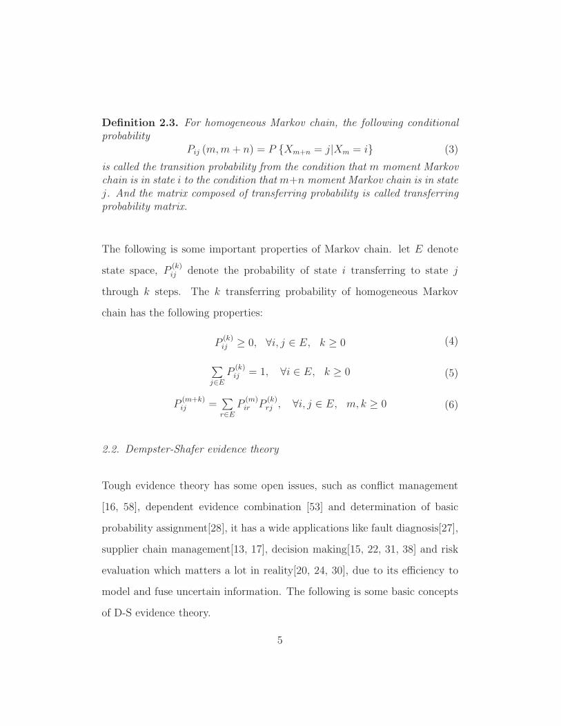
Definition 2.3. For homogeneous Markov chain, the following conditionalprobability

Pij (m,m+ n) = P Xm+n = j|Xm = i (3)

is called the transition probability from the condition that m moment Markovchain is in state i to the condition that m+n moment Markov chain is in statej. And the matrix composed of transferring probability is called transferringprobability matrix.

The following is some important properties of Markov chain. let E denote

state space, P(k)ij denote the probability of state i transferring to state j

through k steps. The k transferring probability of homogeneous Markov

chain has the following properties:

P(k)ij ≥ 0, ∀i, j ∈ E, k ≥ 0 (4)

∑

j∈E

P(k)ij = 1, ∀i ∈ E, k ≥ 0 (5)

P(m+k)ij =

∑

r∈E

P(m)ir P

(k)rj , ∀i, j ∈ E, m, k ≥ 0 (6)

2.2. Dempster-Shafer evidence theory

Tough evidence theory has some open issues, such as conflict management

[16, 58], dependent evidence combination [53] and determination of basic

probability assignment[28], it has a wide applications like fault diagnosis[27],

supplier chain management[13, 17], decision making[15, 22, 31, 38] and risk

evaluation which matters a lot in reality[20, 24, 30], due to its efficiency to

model and fuse uncertain information. The following is some basic concepts

of D-S evidence theory.

5

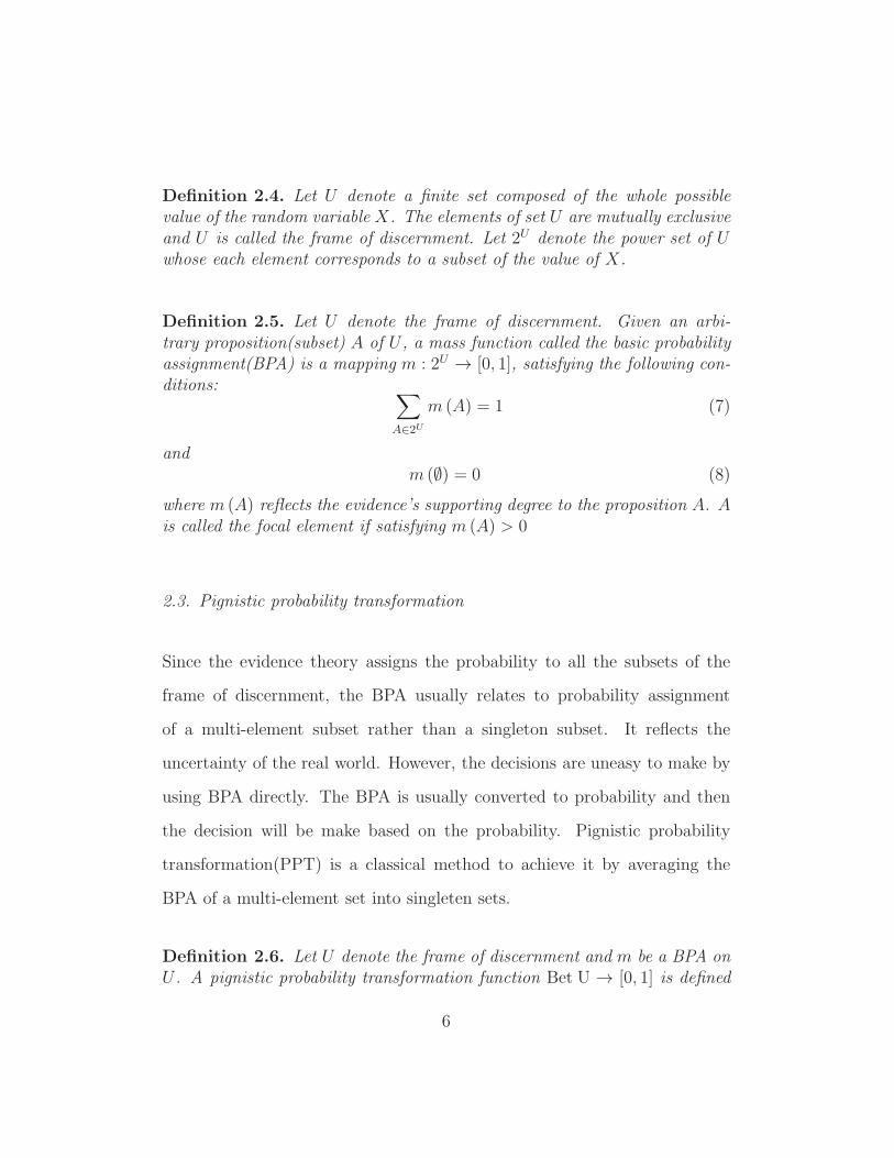
Definition 2.4. Let U denote a finite set composed of the whole possiblevalue of the random variable X. The elements of set U are mutually exclusiveand U is called the frame of discernment. Let 2U denote the power set of Uwhose each element corresponds to a subset of the value of X.

Definition 2.5. Let U denote the frame of discernment. Given an arbi-trary proposition(subset) A of U , a mass function called the basic probabilityassignment(BPA) is a mapping m : 2U → [0, 1], satisfying the following con-ditions:

∑

A∈2U

m (A) = 1 (7)

andm (∅) = 0 (8)

where m (A) reflects the evidence’s supporting degree to the proposition A. Ais called the focal element if satisfying m (A) > 0

2.3. Pignistic probability transformation

Since the evidence theory assigns the probability to all the subsets of the

frame of discernment, the BPA usually relates to probability assignment

of a multi-element subset rather than a singleton subset. It reflects the

uncertainty of the real world. However, the decisions are uneasy to make by

using BPA directly. The BPA is usually converted to probability and then

the decision will be make based on the probability. Pignistic probability

transformation(PPT) is a classical method to achieve it by averaging the

BPA of a multi-element set into singleten sets.

Definition 2.6. Let U denote the frame of discernment and m be a BPA onU . A pignistic probability transformation function Bet U → [0, 1] is defined

6

as:

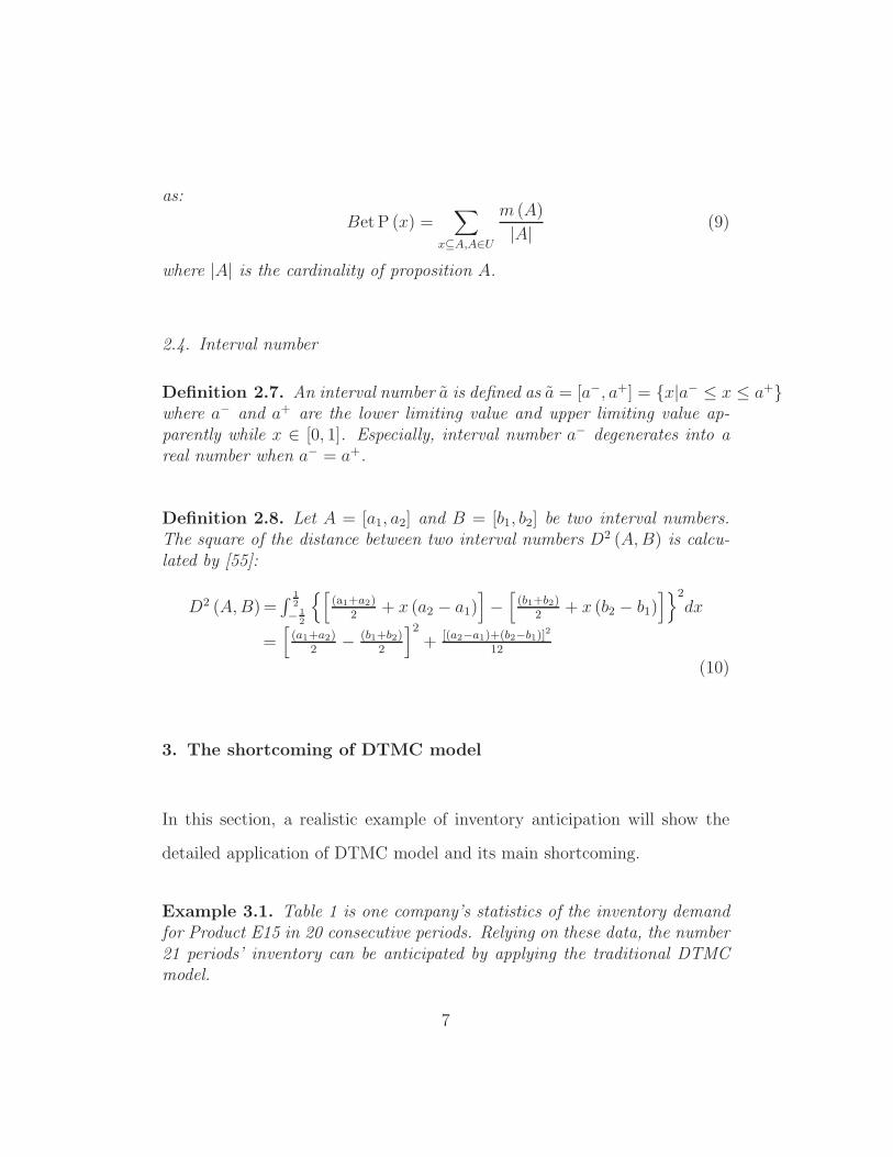
Bet P (x) =∑

x⊆A,A∈U

m (A)

|A|(9)

where |A| is the cardinality of proposition A.

2.4. Interval number

Definition 2.7. An interval number a is defined as a = [a−, a+] = x|a− ≤ x ≤ a+where a− and a+ are the lower limiting value and upper limiting value ap-parently while x ∈ [0, 1]. Especially, interval number a− degenerates into areal number when a− = a+.

Definition 2.8. Let A = [a1, a2] and B = [b1, b2] be two interval numbers.The square of the distance between two interval numbers D2 (A,B) is calcu-lated by [55]:

D2 (A,B) =∫

1

2

−1

2

[

(a1+a2)2

+ x (a2 − a1)]

−[

(b1+b2)2

+ x (b2 − b1)]2

dx

=[

(a1+a2)2

− (b1+b2)2

]2

+ [(a2−a1)+(b2−b1)]2

12

(10)

3. The shortcoming of DTMC model

In this section, a realistic example of inventory anticipation will show the

detailed application of DTMC model and its main shortcoming.

Example 3.1. Table 1 is one company’s statistics of the inventory demandfor Product E15 in 20 consecutive periods. Relying on these data, the number21 periods’ inventory can be anticipated by applying the traditional DTMCmodel.

7

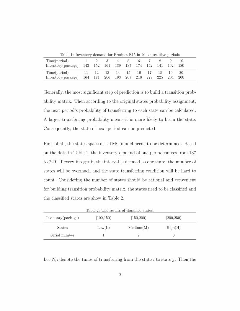
Table 1: Inventory demand for Product E15 in 20 consecutive periods

Time(period) 1 2 3 4 5 6 7 8 9 10Inventory(package) 143 152 161 139 137 174 142 141 162 180

Time(period) 11 12 13 14 15 16 17 18 19 20Inventory(package) 164 171 206 193 207 218 229 225 204 200

Generally, the most significant step of prediction is to build a transition prob-

ability matrix. Then according to the original states probability assignment,

the next period’s probability of transferring to each state can be calculated.

A larger transferring probability means it is more likely to be in the state.

Consequently, the state of next period can be predicted.

First of all, the states space of DTMC model needs to be determined. Based

on the data in Table 1, the inventory demand of one period ranges from 137

to 229. If every integer in the interval is deemed as one state, the number of

states will be overmuch and the state transferring condition will be hard to

count. Considering the number of states should be rational and convenient

for building transition probability matrix, the states need to be classified and

the classified states are show in Table 2.

Table 2: The results of classified states.

Inventory(package) [100,150) [150,200) [200,250)

States Low(L) Medium(M) High(H)

Serial number 1 2 3

Let Nij denote the times of transferring from the state i to state j. Then the

8

following data are obtained.

N11 = 2, N12 = 3, N13 = 0;

N21 = 2, N22 = 4, N23 = 2;

N31 = 0, N32 = 2, N33 = 4.

Let E denote the whole state space. Based on the following equation

Pij = Nij/∑

j∈ENij (11)

the transfer probability matrix can be obtained as:

P =

0.400 0.600 0.000

0.250 0.500 0.250

0.000 0.333 0.667

The inventory of 20th period is 200 packages, belonging to the state medium.

Based on the obtained transfer probability matrix, the state probability as-

signment of the next period is: (L,M,H) = (0.250, 0.500, 0.250) Thus, the

21st period’s state is most likely to be medium with the probability of 0.500.

However, a serious shortcoming exists in this model. If the inventory of the

final period changes from 200 to 201 and the rest data keep the same, then

the new transition probability matrix is obtained as:

P =

0.400 0.600 0.000

0.250 0.500 0.250

0.000 0.167 0.833

9

Because 201 belongs to the state high, the state probability assignment of

21st period turns into: (L,M,H) = (0.000, 0.167, 0.8333). And now the state

high becomes the most likely one with a probability of 0.833, which is much

lager than 0.500. The tiny change in the final period leads to a drastic change

of the prediction, which is obviously irrational. The prediction result should

be close whatever the final inventory is 200 or 201. The reason causing this

situation is that the states are classified by a too crisp critical region. Each

value belongs to a certain state with a probability of 1 completely. Thus, the

prediction result may change drastically in the critical region.

In realistic programs, the value should not correspond to certain state com-

pletely. For example, 200 may belong to the state medium with a probability

of 0.4 while to the state high with a probability of 0.6. Or the value can not

be classified into certain, like it may belong to both medium and high, but

the probability of belong to medium or high is uncertain. Besides, the data

of the previous periods or the current period may be uncertain. In that case,

the states may be hard to classified and the transferring probability matrix

is difficult to build. To address these problems, a new belief Markov model

is proposed.

4. The new belief Markov chain model

The integrated process of building the new belief Markov model is as follow-

ing:

10

Step 1. Determine the state space based on the previous data. Make sure the

number of states is rational and all the states form the frame of discernment

U .

Step 2. Calculate the BPA of the whole periods on the power set of the

discernment 2U based on the distance between interval numbers.

Step 3. Calculate the single-step transferring belief assignment Pij, i, j ∈ 2U

based on the obtained BPA, . And then the transition belief matrix [Pij ] is

built. Pij represents the belief assignment of transferring from proposition i

to proposition j:

Pij =

n−1∑

t=1

(m(i)t·m(j)

t+1)

∑

k∈2U

n−1∑

t=1

(m(i)t·m(k)

t+1), i, j ∈ 2U (12)

where m(i)t represents the assigned belief of proposition i in the t moment,

n represents the length of the Markov chain.

Note 4.1. In classical DTMC model, the transition takes place between basicstates. While in new belief Markov chain model, the transition takes placebetween propositions. In other words, the probability is replaced with BPA.Hence, the original transition probability matrix is replaced with the transitionbelief matrix.

Step 4. Let m = [m (i)] , i ∈ 2U be the BPA of the final period. Then

the assignment of the next period can be obtained by:

m′ = m · [Pij] (13)

11

Step 5. Convert the obtained BPA of the next period m′ into the states

probability assignment [Pij ] , i ∈ 2U by using PPT. And the final predic-

tion result is obtained.

In our model, one of the most significant step is to generate BPA. The detailed

process of generating BPA is shown in the following. First of all, the interval

Figure 1: The flow chart of generating BPA

BPA need to be obtained. The fuzziness and uncertainty existed in realistic

situation can be effectively represented in the form of interval number. And

the crisp number can also be deemed as an interval number like 0.5 can be

seen as [0.5,0.5].

By using Eq.(10), the distance between these interval numbers can be calcu-

lated.

Then the similarity of the interval numbers can be obtained based on the

distance.

Definition 4.1. Let A= [a1, a2] and B= [b1, b2] be two interval numbers. The

12

similarity of the two interval numbers S (A,B) is defined as:

S (A,B) =1

1 +D2 (A,B)(14)

where D (A,B) is the distance between interval number A and B.

When the interval number A equals to B, S (A,B) = 1. According to the

definition, it is easy to know that the larger the difference between A and B

is, the similarity is smaller.

Finally, normalize the obtained similarity and the BPA of interval number is

obtained. An example will show the process in the following.

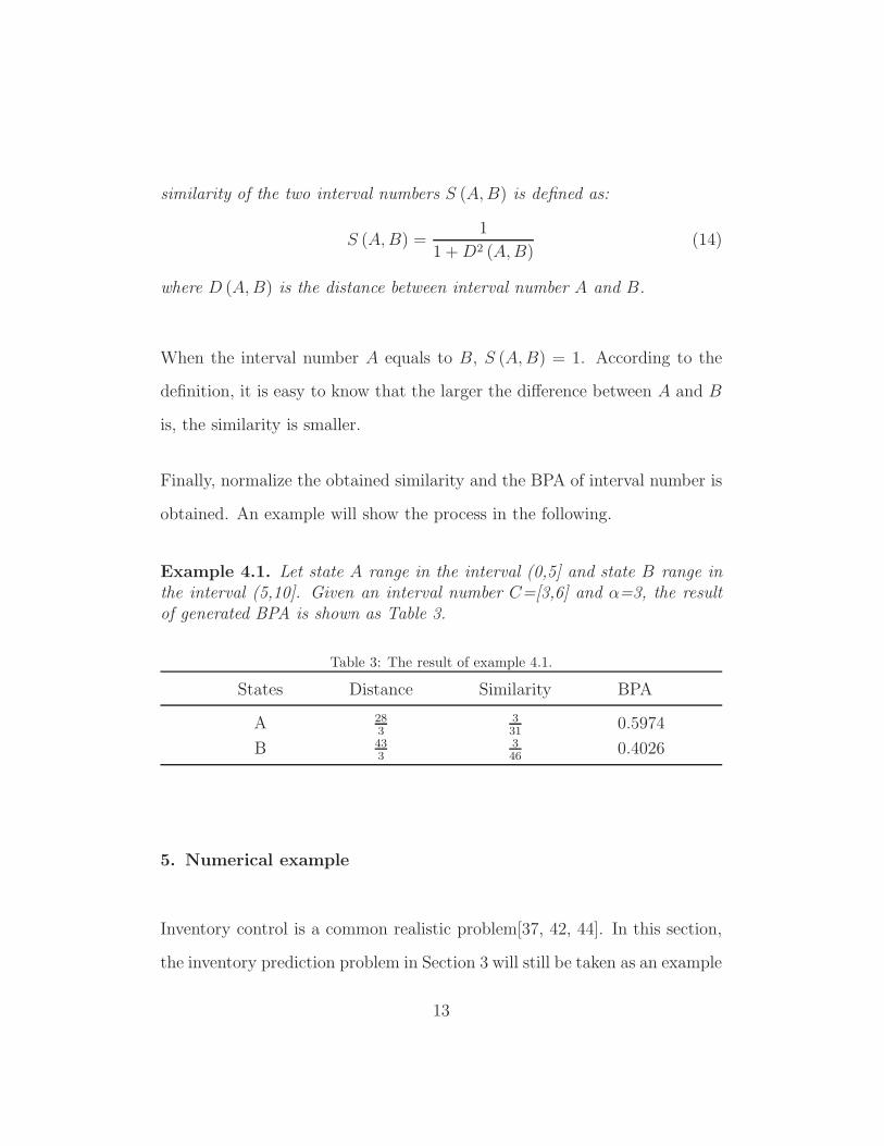
Example 4.1. Let state A range in the interval (0,5] and state B range inthe interval (5,10]. Given an interval number C=[3,6] and α=3, the resultof generated BPA is shown as Table 3.

Table 3: The result of example 4.1.

States Distance Similarity BPA

A 283

331

0.5974

B 433

346

0.4026

5. Numerical example

Inventory control is a common realistic problem[37, 42, 44]. In this section,

the inventory prediction problem in Section 3 will still be taken as an example

13

to show the effectiveness of our model. We assume that some uncertain

information exist in the realistic statistics, some data of inventory demand

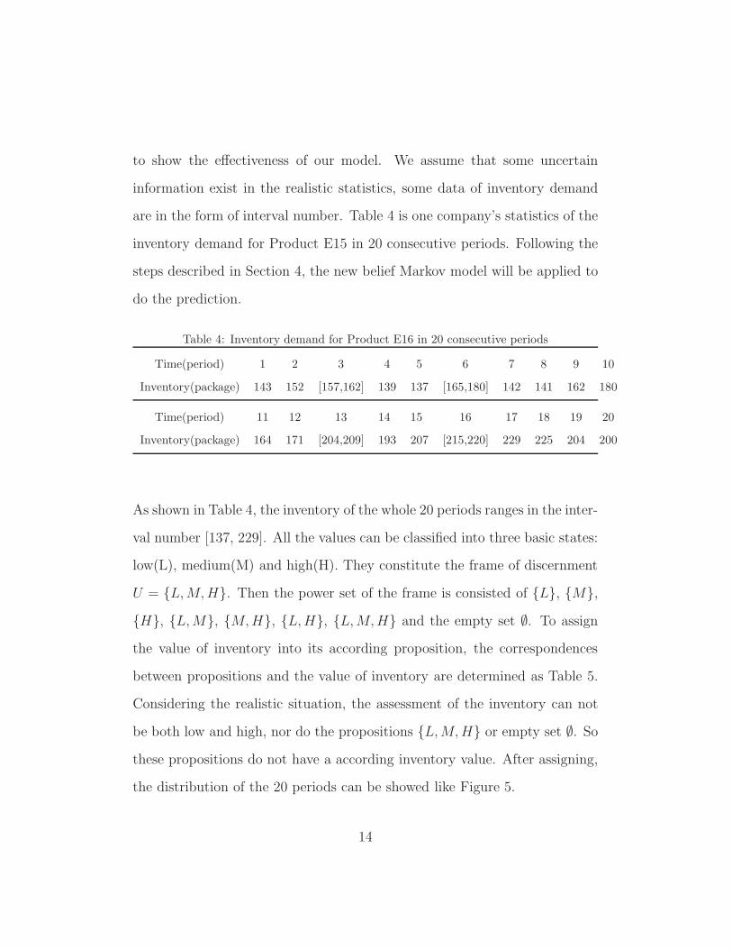
are in the form of interval number. Table 4 is one company’s statistics of the

inventory demand for Product E15 in 20 consecutive periods. Following the

steps described in Section 4, the new belief Markov model will be applied to

do the prediction.

Table 4: Inventory demand for Product E16 in 20 consecutive periods

Time(period) 1 2 3 4 5 6 7 8 9 10

Inventory(package) 143 152 [157,162] 139 137 [165,180] 142 141 162 180

Time(period) 11 12 13 14 15 16 17 18 19 20

Inventory(package) 164 171 [204,209] 193 207 [215,220] 229 225 204 200

As shown in Table 4, the inventory of the whole 20 periods ranges in the inter-

val number [137, 229]. All the values can be classified into three basic states:

low(L), medium(M) and high(H). They constitute the frame of discernment

U = L,M,H. Then the power set of the frame is consisted of L, M,

H, L,M, M,H, L,H, L,M,H and the empty set ∅. To assign

the value of inventory into its according proposition, the correspondences

between propositions and the value of inventory are determined as Table 5.

Considering the realistic situation, the assessment of the inventory can not

be both low and high, nor do the propositions L,M,H or empty set ∅. So

these propositions do not have a according inventory value. After assigning,

the distribution of the 20 periods can be showed like Figure 5.

14

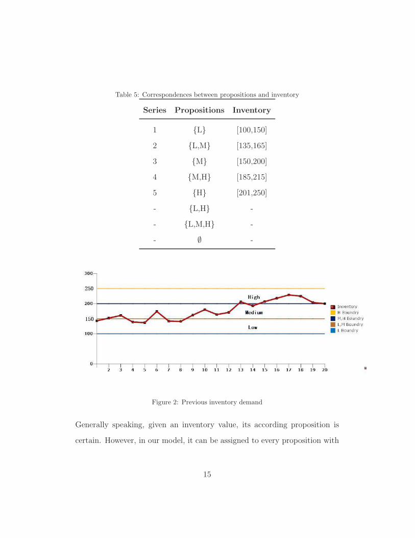
Table 5: Correspondences between propositions and inventory

Series Propositions Inventory

1 L [100,150]

2 L,M [135,165]

3 M [150,200]

4 M,H [185,215]

5 H [201,250]

- L,H -

- L,M,H -

- ∅ -

Figure 2: Previous inventory demand

Generally speaking, given an inventory value, its according proposition is

certain. However, in our model, it can be assigned to every proposition with

15

different probabilities. The probabilities of the assignment are unknown for

now. The BPA cannot be obtained without a certain probability. Thus the

following step is to calculate the probabilities of assignment.

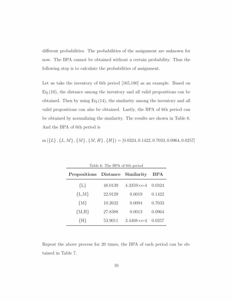
Let us take the inventory of 6th period [165,180] as an example. Based on

Eq.(10), the distance among the inventory and all valid propositions can be

obtained. Then by using Eq.(14), the similarity among the inventory and all

valid propositions can also be obtained. Lastly, the BPA of 6th period can

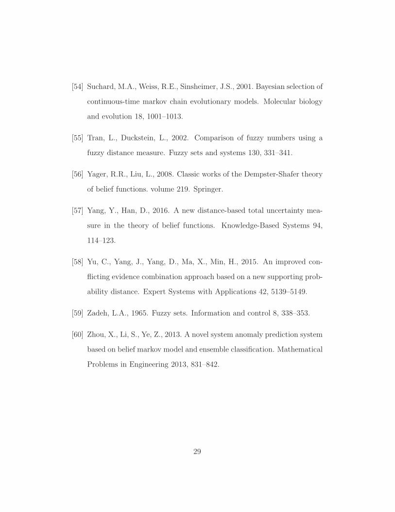
be obtained by normalizing the similarity. The results are shown in Table 6.

And the BPA of 6th period is

m (L , L,M , M , M,H , H) = [0.0324, 0.1422, 0.7033, 0.0964, 0.0257]

Table 6: The BPA of 6th period

Propositions Distance Similarity BPA

L 48.0139 4.3359×e-4 0.0324

L,M 22.9129 0.0019 0.1422

M 10.2632 0.0094 0.7033

M,H 27.8388 0.0013 0.0964

H 53.9011 3.4408×e-4 0.0257

Repeat the above process for 20 times, the BPA of each period can be ob-

tained in Table 7.

16

As shown in Table 7, in this program every BPA is nonzero. Thus the Eq.(12)

can be rewritten as following:

Pij =

n−1∑

t=1

(m(i)t·m(j)

t+1)

∑

k∈2U

n−1∑

t=1

(m(i)t·m(k)

t+1)=

n−1∑

t=1

(m(i)t·m(j)

t+1)n−1∑

t=1

m(i)t

, i, j ∈ 2U (15)

By using Eq.(15), the belief assignment of transferring from one proposition

to another proposition can be calculated. For example, the belief assignment

of transferring from proposition L to proposition L,M is calculated as:

P12 =

n−1∑

t=1

(

m(L)t ·m(L,M)t+1

)

n−1∑

t=1

m(L)t

= 0.4208 (16)

All the obtained transferring belief assignments constitute a 5×5 transition

belief matrix [Pij] as following:

0.1369 0.4208 0.2914 0.1081 0.0427

0.1329 0.4712 0.2559 0.1046 0.0353

0.0923 0.3188 0.2250 0.2769 0.0870

0.0299 0.0938 0.1271 0.5199 0.2292

0.0228 0.0611 0.0895 0.4165 0.4100

The next step is to predict the inventory of the 21st period based on the

BPA of the 20th period and the matrix [Pij ]. As Table 7 shows, the BPA

of the 20th is m (20) = (0.0228, 0.0611, 0.0895, 0.4165, 0.4100). By using the

Eq.(13) the BPA of the 21st is calculated as:

m (21) = m (20) · [Pij] = (0.0379, 0.1214, 0.1368, 0.4792, 0.2247) (17)

17

Finally, use Pignistic probability transformation(Eq.(9)) to transfer the ob-

tained BPA to the probabilities of basic states.

Bet P (L) =0.0379 +0.1214

2= 0.0986

Bet P (M) =0.1214

2+ 0.1368 +

0.4792

2= 0.4371

Bet P (H)=0.4792

2+ 0.2247 = 0.4643

The result is (L,M,H) = (0.0986, 0.4371, 0.4643). Thus, the inventory of

21st period is most likely to be in stage high. The practical inventory demand

for 21st is 223, which is in the state high. Thus, the prediction result confirms

with the reality and is rational.

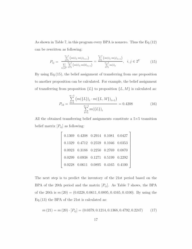
When the inventory of the 20th inventory changes, the result of prediction

also change fluently, which verifies the effectiveness and rationality of our

model. As Figure 3 shows, when the inventory of the 20th period is less than

195, the prediction result is medium. On the contrary, the result is high when

the inventory of the 20th is more than 196. And the line changes fluently.

It reveals that the shortcoming of the classical Markov model mentioned in

Section 3 can be effectively solved in our model. In addition, the comparison

between the prediction and the real situation is shown in Table 8. The

practical inventory of 20th is 200, thus the prediction result is in accord with

the practical situation which prove the effectiveness of our model.

In the following, the comparison between our model and classical DTMC

model is made. Compared with the classical model, the most significant

18

193 194 195 196 197 198 199 200 201 202

The inventory of the 20th period

0

0.1

0.2

0.3

0.4

0.5

0.6

0.7

0.8

The

pre

dict

ed p

roba

bilit

ies

of th

e 21

th p

erio

d LowMediumHigh

Figure 3: The prediction of the 21th period

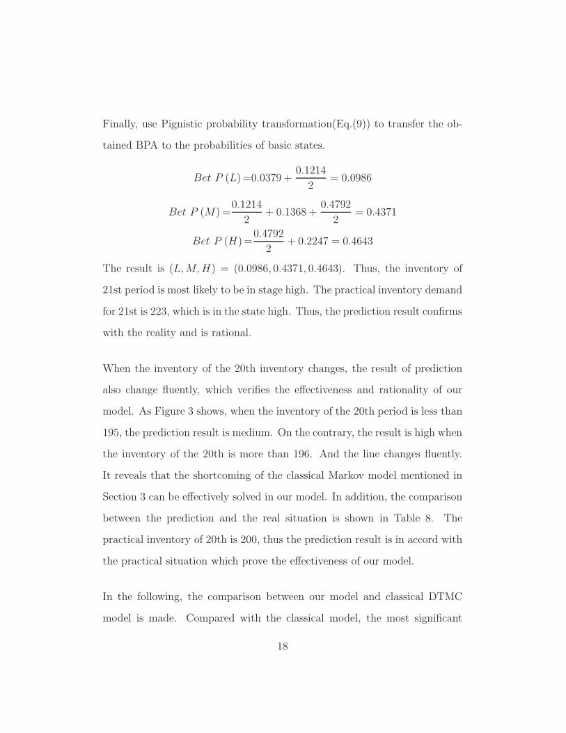
difference of our model is that the state is distributed into each possible state

with a probability. Figure 4 illustrates the methods of state distribution in

different models. The three different models are applied to predict the 21st

inventory demand when the data of 20th fluctuates. As Figure 5 shows,

along the 20th inventory demand changes, the sudden change will exist in

prediction of classical Markov chain model.

As mentioned above, the classical DTMC model can not handle the uncer-

tainty, especially a little change of data may lead to a drastic prediction

result, which is obviously irrational. The increase in the state number may

decrease the trouble caused by uncertainty of states in some degree. How-

ever, a larger data set will be needed to assure it and the problem of drastic

change in prediction is still unavoidable. By contrast, our new belief Markov

19

Figure 4: Comparison of state distribution

chain model can handle these shortcomings effectively. Moreover, the uncer-

tain data like interval number can also be well handled, which proves our

model’s ability of handling uncertain information.

6. Conclusion

In this paper, a new belief Markov chain model is proposed. The shortcom-

ings of classical DTMC model are successfully overcame in this model. The

main advantages of the new model are as following:

1. Stability. The sudden change of prediction result is avoided, namely the

prediction result will change fluently along the slight change of data.

2. The ability of handling uncertain information. Either the uncertainty of

20

state or data can be effectively handled in our model.

3. Flexibility. The different state distribution schemes and basic probability

assignment distribution functions can lead to different results. The setting

can be adjusted according to the realistic situation which reveals the flexi-

bility of our model.

A numerical example of inventory prediction is illustrated in the paper to

show the application of our model. And the prediction result and comparison

prove the effectiveness and rationality of our model.

Acknowledgement

The work is partially supported by National Natural Science Foundation

of China (Grant No. 61671384), Natural Science Basic Research Plan in

Shaanxi Province of China (Program No. 2016JM6018), the Fund of SAST

(Program No. SAST2016083), the Seed Foundation of Innovation and Cre-

ation for Graduate Students in Northwestern Polytechnical University (Pro-

gram No. Z2016122).

References

[1] Alagoz, O., Hsu HSchaefer, A.J., Roberts, M.S., 2010. Markov deci-

sion processes: a tool for sequential decision making under uncertainty.

21

Medical Decision Making 30, 474–483.

[2] Annett, B., Sabine, T., Helge, B., 2010. Twelve years of succession on

sandy substrates in a post-mining landscape: a markov chain analy-

sis. Ecological Applications A Publication of the Ecological Society of

America 20, 1136–47.

[3] Arenas, A., Borge-Holthoefer, J., Meloni, S., Moreno, Y., et al., 2010.

Discrete-time markov chain approach to contact-based disease spreading

in complex networks. EPL (Europhysics Letters) 89, 38009.

[4] Avrachenkov, K.E., Sanchez, E., 2002. Fuzzy markov chains and

decision-making. Fuzzy Optimization and Decision Making 1, 143–159.

[5] Aziz, A., Sanwal, K., Singhal, V., Brayton, R., 2000. Model-checking

continuous-time markov chains. ACM Transactions on Computational

Logic (TOCL) 1, 162–170.

[6] Benavoli, A., Chisci, L., Farina, A., Ristic, B., 2008. Modelling uncertain

implication rules in evidence theory, in: Information Fusion, 2008 11th

International Conference on, IEEE. pp. 1–7.

[7] Boudaren, M.E.Y., An, L., Pieczynski, W., 2016. Dempster-shafer fu-

sion of evidential pairwise markov fields. IEEE Transactions on Fuzzy

Systems 74, 13–29.

[8] Boujelben, M.A., De Smet, Y., Frikha, A., Chabchoub, H., 2009. Build-

ing a binary outranking relation in uncertain, imprecise and multi-

22

experts contexts: The application of evidence theory. International

journal of approximate reasoning 50, 1259–1278.

[9] Buckley, J.J., 2005. Fuzzy markov chains. Fuzzy Probabilities: New

Approach and Applications , 71–83.

[10] Chou, C.C., 2016. A generalized similarity measure for fuzzy numbers.

Journal of Intelligent & Fuzzy Systems 30, 1147–1155.

[11] Darling, D.A., Siegert, A.J.F., 1953. The first passage problem for a

continuous markov process. Annals of Mathematical Statistics 24, 624–

639.

[12] De Korvin, A., Kleyle, R., 1998. Expected transition costs based on a

markov model having fuzzy states with an application to policy selection.

Stochastic analysis and applications 16, 51–64.

[13] Deng, X., Hu, Y., Deng, Y., Mahadevan, S., 2014a. Supplier selection

using AHP methodology extended by d numbers. Expert Systems with

Applications 41, 156–167.

[14] Deng, X., Liu, Q., Deng, Y., 2015. Newborns prediction based on a

belief markov chain model. Applied Intelligence 43, 1–14.

[15] Deng, X., Lu, X., Chan, F.T.S., Sadiq, R., Mahadevan, S., Deng, Y.,

2014b. D-cfpr: D numbers extended consistent fuzzy preference rela-

tions. Knowledge-Based Systems 73, 61C68.

23

[16] Deng, Y., 2015. Generalized evidence theory. Applied Intelligence 43,

530–543.

[17] Deng, Y., Chan, F.T.S., 2011. A new fuzzy dempster mcdm method and

its application in supplier selection. Expert Systems with Applications

38, 9854–9861.

[18] Dou, R., Zong, C., Li, M., 2016. An interactive genetic algorithm with

the interval arithmetic based on hesitation and its application to achieve

customer collaborative product configuration design. Applied Soft Com-

puting 38, 384–394.

[19] Farahat, A., 2010. Markov stochastic technique to determine galactic

cosmic ray sources distribution. Journal of Astrophysics and Astronomy

31, 81–88.

[20] Feng, N., Yu, X., Dou, R., Pan, B., 2015. Managing risk for business

processes: A fuzzy based multi-agent system. Journal of Intelligent &

Fuzzy Systems 29, 2717–2726.

[21] Fraedrich, K., Muller, K., 1983. On single station forecasting: Sunshine

and rainfall markov chains. Beitr. Phys. Atmos 56, 208–134.

[22] Fu, C., Yang, J.B., Yang, S.L., 2015. A group evidential reasoning

approach based on expert reliability. European Journal of Operational

Research 246, 886–893.

24

[23] Fu, J.C., Koutras, M.V., 1994. Distribution theory of runs: A markov

chain approach. Journal of the American Statistical Association 18,

1050–1058.

[24] Guo, J., 2016. A risk assessment approach for failure mode and effects

analysis based on intuitionistic fuzzy sets and evidence theory. Journal

of Intelligent & Fuzzy Systems 30, 869–881.

[25] Jiang, C., Han, X., Liu, G., Liu, G., 2008. A nonlinear interval number

programming method for uncertain optimization problems. European

Journal of Operational Research 188, 1–13.

[26] Jiang, W., Luo, Y., Qin, X., Zhan, J., 2015. An improved method

to rank generalized fuzzy numbers with different left heights and right

heights. Journal of Intelligent & Fuzzy Systems 28, 2343–2355.

[27] Jiang, W., Wei, B., Xie, C., Zhou, D., 2016a. An evidential sensor fusion

method in fault diagnosis. Advances in Mechanical Engineering 8, 1–7.

[28] Jiang, W., Zhan, J., Zhou, D., Li, X., 2016b. A method to determine

generalized basic probability assignment in the open world. Mathemat-

ical Problems in Engineering 2016, 1–11.

[29] Jin, Y., Xie, Z., Chen, J., Chen, E., 2015. Phev power distribution

fuzzy logic control strategy based on prediction. Journal of Zhejiang

University of Technology 43, 97–102.

25

[30] Kabir, G., Tesfamariam, S., Francisque, A., Sadiq, R., 2015. Evaluat-

ing risk of water mains failure using a bayesian belief network model.

European Journal of Operational Research 240, 220–234.

[31] Kang, B., Deng, Y., Sadiq, R., Mahadevan, S., 2012. Evidential cogni-

tive maps. Knowledge-Based Systems 35, 77–86.

[32] Kemeny, J.G., Snell, J.L., 1960. Finite markov chain. American Math-

ematical Monthly 67.

[33] Kleyle, R., De Korvin, A., 1997. Transition probabilities for markov

chains having fuzzy states. Stochastic analysis and applications 15, 527–

546.

[34] Komorowski, T., Szarek, T., 2010. On ergodicity of some markov pro-

cesses. Annals of Probability 38, pgs. 1401–1443.

[35] Krogh, A., Larsson, B., Von Heijne, G., Sonnhammer, E.L., 2001. Pre-

dicting transmembrane protein topology with a hidden markov model:

application to complete genomes. Journal of molecular biology 305,

567–580.

[36] Lange, K., 2010. Discrete-time markov chains, in: Applied Probability.

Springer, pp. 151–185.

[37] Levi, R., Pl, M., Roundy, R., Shmoys, D.B., 2005. Approximation Al-

gorithms for Stochastic Inventory Control Models. Springer Berlin Hei-

delberg.

26

[38] Li, Y., Chen, J., Ye, F., Liu, D., 2016. The improvement of ds evidence

theory and its application in ir/mmw target recognition. Journal of

Sensors 2016, 1–15.

[39] Liu, C., Tian, Y.M., Wang, X.H., 2011. Study of rainfall prediction

model based on gm (1, 1) - markov chain, in: Water Resource and

Environmental Protection (ISWREP), 2011 International Symposium

on, pp. 744–747.

[40] Lu, Y., Zhang, M., Yu, T., Qu, M., Lu, Y., Zhang, M., Yu, T., Qu,

M., 2014. Application of markov prediction method in the decision of

insurance company. lemcs-14 .

[41] Mar, J., Anto?anzas, F., Pradas, R., Arrospide, A., 2010. Probabilistic

markov models in economic evaluation of health technologies: a practical

guide. Gaceta Sanitaria 24, 209–214.

[42] Memari, A., Rahim, A.R.B.A., Ahmad, R.B., 2014. Production Plan-

ning and Inventory Control in Automotive Supply Chain Networks.

[43] Navaei, 2010. Markov chain for multiple hypotheses testing and iden-

tification of distributions for one object. Pakistan Journal of Statistics

26, 557–562.

[44] Ozbay, K., Ozguven, E.E., 2007. Stochastic Humanitarian Inventory

Control Model for Disaster Planning.

27

[45] Pieczynski, W., Benboudjema, D., 2006. Multisensor triplet markov

fields and theory of evidence. Image & Vision Computing 24, 61–69.

[46] Privault, N., 2013. Discrete-time markov chains, in: Understanding

Markov Chains. Springer, pp. 77–94.

[47] Rabiner, L.R., Juang, B.H., 1986. An introduction to hidden markov

models. ASSP Magazine, IEEE 3, 4–16.

[48] Samet, H., Mojallal, A., 2014. Enhancement of electric arc furnace re-

active power compensation using grey-markov prediction method. Gen-

eration, Transmission & Distribution, IET 8, 1626–1636.

[49] Shafer, G., et al., 1976. A mathematical theory of evidence. volume 1.

Princeton university press Princeton.

[50] Song, Y., Wang, X., Lei, L., Yue, S., 2016. Uncertainty measure for

interval-valued belief structures. Measurement 80, 241–250.

[51] Soubaras, H., 2009. An Evidential Measure of Risk in Evidential Markov

Chains. Springer Berlin Heidelberg.

[52] Soubaras, H., 2010. On evidential markov chains. Studies in Fuzziness

& Soft Computing 249, 247–264.

[53] Su, X., Mahadevan, S., Han, W., Deng, Y., 2016. Combining dependent

bodies of evidence. Applied Intelligence 44, 634–644.

28

[54] Suchard, M.A., Weiss, R.E., Sinsheimer, J.S., 2001. Bayesian selection of

continuous-time markov chain evolutionary models. Molecular biology

and evolution 18, 1001–1013.

[55] Tran, L., Duckstein, L., 2002. Comparison of fuzzy numbers using a

fuzzy distance measure. Fuzzy sets and systems 130, 331–341.

[56] Yager, R.R., Liu, L., 2008. Classic works of the Dempster-Shafer theory

of belief functions. volume 219. Springer.

[57] Yang, Y., Han, D., 2016. A new distance-based total uncertainty mea-

sure in the theory of belief functions. Knowledge-Based Systems 94,

114–123.

[58] Yu, C., Yang, J., Yang, D., Ma, X., Min, H., 2015. An improved con-

flicting evidence combination approach based on a new supporting prob-

ability distance. Expert Systems with Applications 42, 5139–5149.

[59] Zadeh, L.A., 1965. Fuzzy sets. Information and control 8, 338–353.

[60] Zhou, X., Li, S., Ye, Z., 2013. A novel system anomaly prediction system

based on belief markov model and ensemble classification. Mathematical

Problems in Engineering 2013, 831–842.

29

Table 7: The BPA of 20 periodsPPPPPPPPPPPPPP

Period

PropositionsL L,M M M,H H

1 0.1758 0.7137 0.0709 0.0268 0.0127

2 0.0713 0.8047 0.0855 0.0270 0.0115

3 0.0694 0.6379 0.2186 0.0540 0.0202

4 0.2988 0.5814 0.0747 0.0302 0.0149

5 0.3728 0.5072 0.0738 0.0307 0.0155

6 0.0324 0.1422 0.7033 0.0964 0.0257

7 0.2023 0.6841 0.0724 0.0278 0.0134

8 0.2319 0.6518 0.0736 0.0288 0.0139

9 0.0750 0.5224 0.2998 0.0756 0.0272

10 0.0375 0.1220 0.5379 0.2501 0.0524

11 0.0720 0.4456 0.3636 0.0883 0.0304

12 0.0296 0.0981 0.6195 0.2111 0.0417

13 0.0108 0.0224 0.0648 0.7630 0.1390

14 0.0183 0.0452 0.1715 0.6959 0.0692

15 0.0131 0.0270 0.0753 0.7191 0.1654

16 0.0158 0.0295 0.0691 0.3467 0.5389

17 0.0144 0.0249 0.0514 0.1716 0.7377

18 0.0141 0.0249 0.0535 0.2025 0.7050

19 0.0113 0.0241 0.0712 0.7845 0.1088

20 0.0108 0.0240 0.0773 0.8151 0.0728

30

Table 8: Comparison between prediction and practical situation

Inventory 193 194 195 196 197

Prediction result(Probability) M(0.4577) M(0.4511) M(0.4479) H(0.4454) H(0.4516)

Practical situation H

Inventory 198 199 200 201 202

Prediction result(Probability) H(0.4568) H(0.4609) H(0.4643) H(0.4670) H(0.4692)

Practical situation H

31

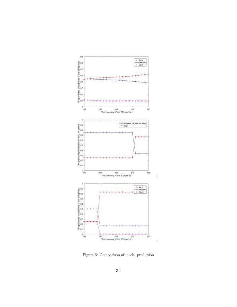
Figure 5: Comparison of model prediction

32