Am

DJa

b

c

a

ARRAA

KSMPMS

1

eudipdoratasmmfro

0d

Chemical Engineering and Processing 48 (2009) 1495–1505

Contents lists available at ScienceDirect

Chemical Engineering and Processing:Process Intensification

journa l homepage: www.e lsev ier .com/ locate /cep

2D Markov chain for modelling powder mixing in alternately revolving staticixers of Sysmix® type

enis Ponomareva, Vadim Mizonova, Henri Berthiauxb,∗, Cendrine Gatumelb,anos Gyenisc, Elena Barantsevaa

Department of Applied Mathematics, ISPEU, Rabfakovskaya 34, 153003 Ivanovo, RussiaRAPSODEE Centre, École des Mines d’Albi, FRE CNRS 3213, campus jarlard, route de Teillet, 81013 Albi, FranceRIChPE FIT, University of Pannonia, Egyetem u. 2, H-8200 Veszprem, Hungary

r t i c l e i n f o

rticle history:eceived 2 April 2009eceived in revised form 5 October 2009ccepted 6 October 2009vailable online 12 October 2009

a b s t r a c t

A two-dimensional model of the flow and mixing of particulate solids has been developed on the basis ofthe Markov chain theory for an alternately revolving static mixer of Sysmix® type. In such a system, mixingoccurs in both vertical and horizontal directions. Simulations are presented here to investigate the effect ofthe initial loading of the components, as well as the effect of the values of the transition probabilities that

eywords:tatic mixerixing kinetics

owder mixingarkov chains

tochastic process

constitute the main parameters of the model. It is shown that a horizontal arrangement of the componentsalways leads to better mixture quality and improved mixing kinetics. This research is presented for non-segregating mixtures, as well as potentially segregating mixtures, for which the empirically well-knownoscillations in variance are represented by the model. Results suggest that there is a rational way ofapproaching a static-mixing problem with regard to the initial loading of the component and the optimalnumber of revolutions. Comparison of model results with experimental data published previously for aSysmix® apparatus contributes to validating the viability of the model.

. Introduction

Choosing a powder mixer is a complex and time-consumingxercise for a chemical engineer. To select a simple distillation col-mn, the engineer will probably spend several hours deciding onimensions and characteristics, and a further day or more consult-

ng vendors and purchasing the column. To select an appropriateowder mixer, the time required may be up to several months. Thiselay in the decision-making process can be explained by the lackf knowledge of powder characterization in general, and of powderheology in particular. As a consequence, the range of technologiesvailable for mixing powders is extremely large. The shape of aumbler mixer may be a cylinder, a sphere, a cube, a double-cone,double cylinder. The axis of rotation may differ from the axis of

ymmetry, and inserts can be included in the design. Convectiveixers all differ from each other by the shape of the stirrer, which

ay be a ribbon, paddles mounted on a shaft, blades mounted on a

rame, multiple screws, or a planetary motion with various axis ofotation—all this being combined with the different possible shapesf the mixing vessel. The broad category of “home-made” mixers,

∗ Corresponding author.E-mail address: berthiau@enstimac.fr (H. Berthiaux).

255-2701/$ – see front matter © 2009 Elsevier B.V. All rights reserved.oi:10.1016/j.cep.2009.10.004

© 2009 Elsevier B.V. All rights reserved.

of which container-mixers form a part, are subject to numerousfailures that occur in scale-up and design procedures.

Depending on the manufacturing possibilities, such as the avail-ability of spare parts, other alternatives like fluidised-bed mixers,static or silo mixers may be envisaged. In these types, the generalmotion of the particles is induced by gravity and the process oper-ates by multiple passes or by the alternate revolving of the mixer.Insertions that are placed inside the vessel provoke dispersion ofthe particles (see Fig. 1). Static mixers provide a greater contactarea between particles of different nature, which is a preliminaryto the achievement of a finer-scale mixture. They could probablygive good results as premix units, for example at the inlet of a con-tinuous plough mixer, but have never been studied from this pointof view.

Modelling of powder mixing and flow is a very valuableapproach to the understanding of the collective and individ-ual motion of particulates, and therefore may prove useful inimproving mixer design. Distinct Element Models (DEMs) havebeen developed and applied to real mixing cases since the mid-nineteen nineties. DEMs are based on calculating particle–particle

and particle–wall interactions, a procedure that requires the detec-tion of the contacts between particles, which can be difficult ifthese are of non-spherical shape [1]. This procedure limits consid-erably the number of elements (particles) that need to be taken intoaccount in the simulation and has led most researchers to develop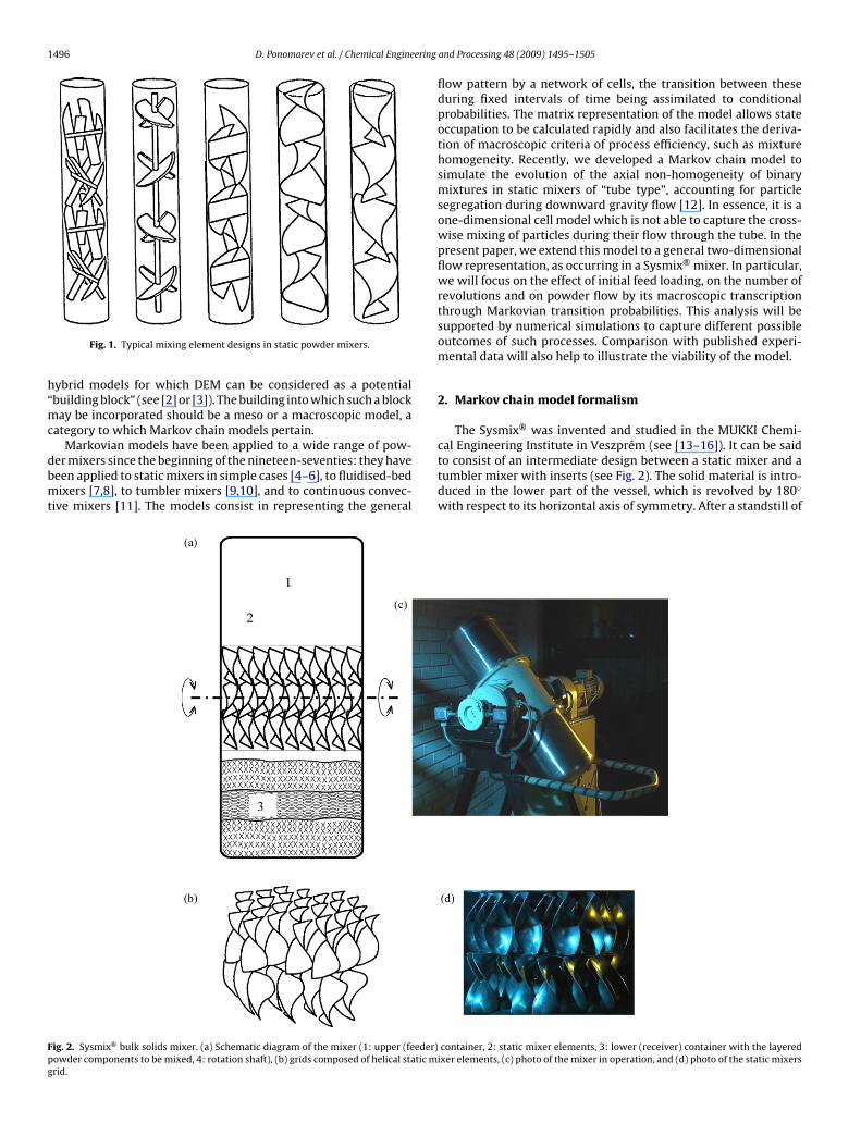

1496 D. Ponomarev et al. / Chemical Engineering

h“mc

dbmt

Fpg

Fig. 1. Typical mixing element designs in static powder mixers.

ybrid models for which DEM can be considered as a potentialbuilding block” (see [2] or [3]). The building into which such a blockay be incorporated should be a meso or a macroscopic model, a

ategory to which Markov chain models pertain.

Markovian models have been applied to a wide range of pow-

er mixers since the beginning of the nineteen-seventies: they haveeen applied to static mixers in simple cases [4–6], to fluidised-bedixers [7,8], to tumbler mixers [9,10], and to continuous convec-

ive mixers [11]. The models consist in representing the general

ig. 2. Sysmix® bulk solids mixer. (a) Schematic diagram of the mixer (1: upper (feeder)owder components to be mixed, 4: rotation shaft), (b) grids composed of helical static mrid.

and Processing 48 (2009) 1495–1505

flow pattern by a network of cells, the transition between theseduring fixed intervals of time being assimilated to conditionalprobabilities. The matrix representation of the model allows stateoccupation to be calculated rapidly and also facilitates the deriva-tion of macroscopic criteria of process efficiency, such as mixturehomogeneity. Recently, we developed a Markov chain model tosimulate the evolution of the axial non-homogeneity of binarymixtures in static mixers of “tube type”, accounting for particlesegregation during downward gravity flow [12]. In essence, it is aone-dimensional cell model which is not able to capture the cross-wise mixing of particles during their flow through the tube. In thepresent paper, we extend this model to a general two-dimensionalflow representation, as occurring in a Sysmix® mixer. In particular,we will focus on the effect of initial feed loading, on the number ofrevolutions and on powder flow by its macroscopic transcriptionthrough Markovian transition probabilities. This analysis will besupported by numerical simulations to capture different possibleoutcomes of such processes. Comparison with published experi-mental data will also help to illustrate the viability of the model.

2. Markov chain model formalism

The Sysmix® was invented and studied in the MUKKI Chemi-

cal Engineering Institute in Veszprém (see [13–16]). It can be saidto consist of an intermediate design between a static mixer and atumbler mixer with inserts (see Fig. 2). The solid material is intro-duced in the lower part of the vessel, which is revolved by 180◦

with respect to its horizontal axis of symmetry. After a standstill of

container, 2: static mixer elements, 3: lower (receiver) container with the layeredixer elements, (c) photo of the mixer in operation, and (d) photo of the static mixers

D. Ponomarev et al. / Chemical Engineering and Processing 48 (2009) 1495–1505 1497

ng sec

airiabtactoftdpt

2

rcswicupta

id“

123

s

same layers as in the loading container.We now focus on the mixing zone and illustrate the strategy of

building a so-called “2D-model” by considering the simple case ofa 3 × 3 two-dimensional network of cells as shown in Fig. 4. Thecells are considered to occupy identical volumes in the mixer, but

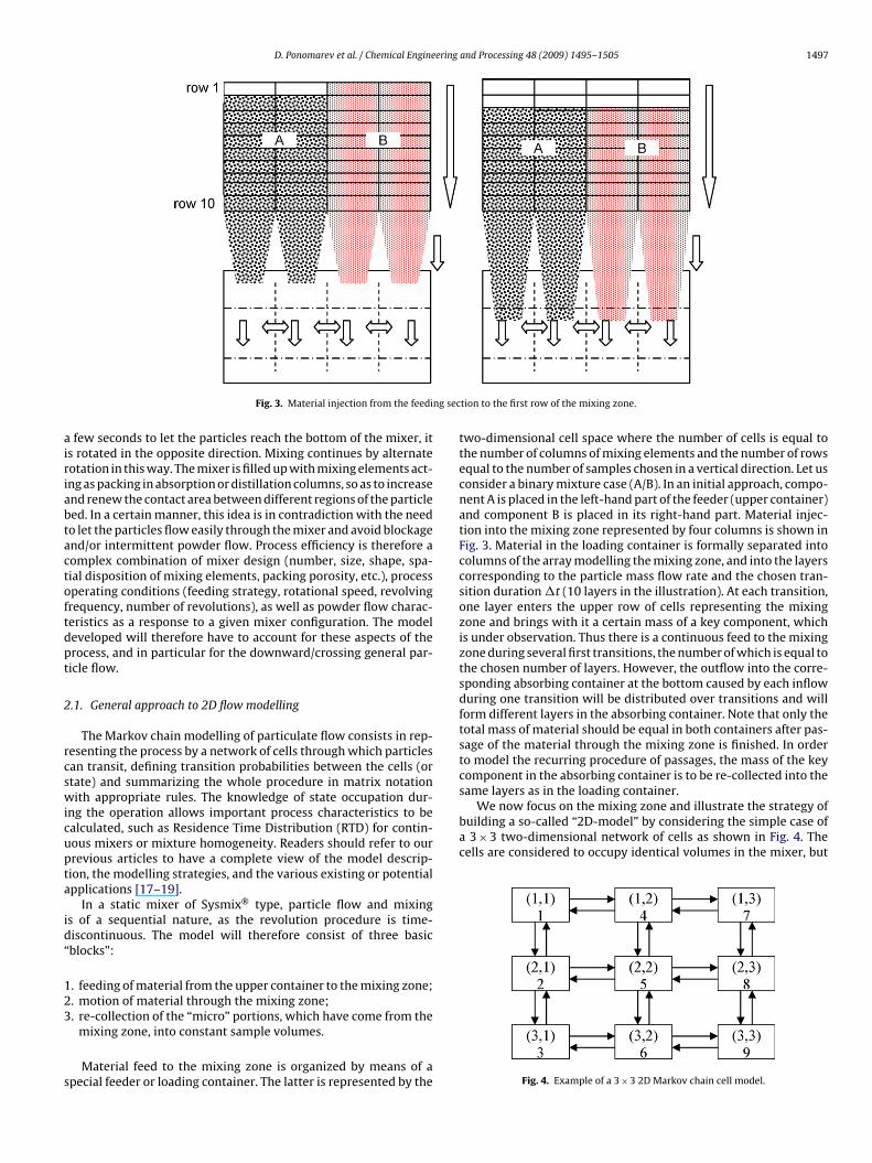
Fig. 3. Material injection from the feedi

few seconds to let the particles reach the bottom of the mixer, its rotated in the opposite direction. Mixing continues by alternateotation in this way. The mixer is filled up with mixing elements act-ng as packing in absorption or distillation columns, so as to increasend renew the contact area between different regions of the particleed. In a certain manner, this idea is in contradiction with the needo let the particles flow easily through the mixer and avoid blockagend/or intermittent powder flow. Process efficiency is therefore aomplex combination of mixer design (number, size, shape, spa-ial disposition of mixing elements, packing porosity, etc.), processperating conditions (feeding strategy, rotational speed, revolvingrequency, number of revolutions), as well as powder flow charac-eristics as a response to a given mixer configuration. The modeleveloped will therefore have to account for these aspects of therocess, and in particular for the downward/crossing general par-icle flow.

.1. General approach to 2D flow modelling

The Markov chain modelling of particulate flow consists in rep-esenting the process by a network of cells through which particlesan transit, defining transition probabilities between the cells (ortate) and summarizing the whole procedure in matrix notationith appropriate rules. The knowledge of state occupation dur-

ng the operation allows important process characteristics to bealculated, such as Residence Time Distribution (RTD) for contin-ous mixers or mixture homogeneity. Readers should refer to ourrevious articles to have a complete view of the model descrip-ion, the modelling strategies, and the various existing or potentialpplications [17–19].

In a static mixer of Sysmix® type, particle flow and mixings of a sequential nature, as the revolution procedure is time-iscontinuous. The model will therefore consist of three basicblocks”:

. feeding of material from the upper container to the mixing zone;

. motion of material through the mixing zone;

. re-collection of the “micro” portions, which have come from themixing zone, into constant sample volumes.

Material feed to the mixing zone is organized by means of apecial feeder or loading container. The latter is represented by the

tion to the first row of the mixing zone.

two-dimensional cell space where the number of cells is equal tothe number of columns of mixing elements and the number of rowsequal to the number of samples chosen in a vertical direction. Let usconsider a binary mixture case (A/B). In an initial approach, compo-nent A is placed in the left-hand part of the feeder (upper container)and component B is placed in its right-hand part. Material injec-tion into the mixing zone represented by four columns is shown inFig. 3. Material in the loading container is formally separated intocolumns of the array modelling the mixing zone, and into the layerscorresponding to the particle mass flow rate and the chosen tran-sition duration �t (10 layers in the illustration). At each transition,one layer enters the upper row of cells representing the mixingzone and brings with it a certain mass of a key component, whichis under observation. Thus there is a continuous feed to the mixingzone during several first transitions, the number of which is equal tothe chosen number of layers. However, the outflow into the corre-sponding absorbing container at the bottom caused by each inflowduring one transition will be distributed over transitions and willform different layers in the absorbing container. Note that only thetotal mass of material should be equal in both containers after pas-sage of the material through the mixing zone is finished. In orderto model the recurring procedure of passages, the mass of the keycomponent in the absorbing container is to be re-collected into the

Fig. 4. Example of a 3 × 3 2D Markov chain cell model.

1 ering

to“p

S

s

S

w

S

batnrbts

P

dmtpmsnFesfmaab

dorfimtcaabb

498 D. Ponomarev et al. / Chemical Engine

he corresponding particle masses may be different. The particlesf a certain component A of a binary mixture can occupy the cellij” with a frequency, or a concentration, sij. Consequently, the staterobability distribution along cells can be defined by the matrix Sm:

m =[

s11 s12 s13s21 s22 s23s31 s32 s33

](1)

In order to perform the next matrix operations, model cellshould be renumbered in a sequence shown in Fig. 4:

m =[

s1 s4 s7s2 s5 s8s3 s6 s9

](2)

hich should in turn be transformed into the state vector:

=

⎡⎢⎢⎣

s1s2. . .s8s9

⎤⎥⎥⎦ (3)

The mixing zone is represented by a matrix of transition proba-ilities of size 9 × 9, since mixing occurs in two directions, verticalnd horizontal. Each column contains transition probabilities fromhe given cell to the neighbouring cells according to its direct unaryumeration. The main diagonal is concerned with probabilities ofemaining in cells during one transition. These probabilities cane obtained by subtracting the sum of transition probabilities tohe neighbouring cells from 1. The probabilities of such transitionshould be placed in the columns of the matrix:

=

⎡⎢⎢⎢⎢⎢⎢⎢⎣

1 → 1 2 → 1 0 4 → 1 0 0 0 0 01 → 2 2 → 2 3 → 2 0 5 → 1 0 0 0 0

0 2 → 3 3 → 3 0 0 6 → 3 0 0 01 → 4 0 0 4 → 4 5 → 4 0 7 → 4 0 0

0 2 → 5 0 4 → 5 5 → 5 6 → 5 0 8 → 5 00 0 3 → 6 0 5 → 6 6 → 6 0 0 9 → 60 0 0 4 → 7 0 0 7 → 7 8 → 7 00 0 0 0 5 → 8 0 7 → 8 8 → 8 9 → 80 0 0 0 0 6 → 9 0 8 → 9 9 → 9

⎤⎥⎥⎥⎥⎥⎥⎥⎦(4)

Let us consider the mixing zone of a Sysmix®-type mixer in moreetail. It is made of mixing elements, axially installed inside theixer. Each element is of helical shape and is slewed around its ver-

ical axis by 90◦ relative to the previous and subsequent elementslaced above and below the element in question. Consequently,aterial flow will occur along the two sides of each mixing element

o that the material goes to the bottom of this element and to othereighbouring zones. A cell model of the process is represented inig. 5. Each cell represents one side of a mixing element, the mixingffect happening in an axial direction at the interfaces between theuccessive cells. A vertical series of helical mixing elements is there-ore represented by two columns of cells in the model. Crosswise

ixing arises in the mixer because of particle rebound or inter-ction with the mixing elements. In the model, this is taken intoccount by only allowing transitions in the horizontal directionetween the cells that are not separated by an element.

Finally, material is collected in the lower container, whoseimensions are identical to those of the upper container. Particlesf each component arrive in the lower part of the vessel after theevolution of the mixer during the standstill period. It is thereforelled according to the flow behaviour of each component in theixing zone. Each column of the lower container may then con-

ain a different powder volume, and each cell may exhibit different

oncentrations in a specific component as long as mixture is notchieved at this scale of scrutiny. As the mixing procedure oper-tes by turning the whole mixer body around its horizontal axisy 180◦, the lower container serves as a feed for the next passageeing turned upside down. The process can then be repeated and

and Processing 48 (2009) 1495–1505

its dynamics can be followed by the Markov chain representationwith appropriate rules of calculation.

2.2. Transition matrix and process dynamics

The dynamics of material motion through the mixing zone isdefined by the following matrix equation:

Sk+1 = P(Sk + S(k)f

) (5)

In the above equation, P is the transition matrix describing theexchanges of material in the mixing zone, S is the state columnvector for the mixing zone and S(k)

fis a column vector represent-

ing material feed. The latter can represent a step feed into the firstrow of the model as in the first pass of the present case, but can alsorepresent a slot-type feed, a sinusoidal feed, a staged feed along themixer’s length and so forth. For a mixing zone consisting of a singlecolumn, this vector would be of size n × 1. For m mixing columns,its size is n × m and it is built by placing the feed vectors to eachcolumn one under another. The matrix of transition probabilitiesP is a block matrix, and has the following form according to themodel scheme presented:

P =

⎡⎢⎢⎢⎢⎢⎢⎢⎢⎣

P11 P12 Z Z Z Z

P21 P22 P23 Z Z Z

Z P32 P33 P34 Z Z

Z Z P43 P44 P45 Z

Z Z Z P54 P55 P56

Z Z Z Z P65 P66

⎤⎥⎥⎥⎥⎥⎥⎥⎥⎦

(6)

The matrices Pij, placed above the main diagonal of P are respon-sible for material motion from the right columns to the left ones, i.e.,from the jth columns to the (j − 1)th as only crosswise flow existsbetween adjacent elements. Similarly, the matrices Pji placed belowthe main diagonal are responsible for material motion from the leftcolumns to the right ones, i.e., from the jth columns to the (j + 1)th.Matrices Pii represent particle flow “inside” the ith column, and Zis a zero matrix of size 4 × 4. It should be noted that the indexing ofthe sub-matrices in the above does not coincide with the indexingof mixing cells in the model.

The matrix of transition probabilities for the vertical helical mix-ing sets of Fig. 5 can be seen in Fig. 6 in accordance with the aboveremarks. If the probability to stay in a cell ps is the same for a compo-nent whichever cell is considered, if pc is the probability to transit inthe horizontal direction, and pd is the probability to transit in thevertical direction, the transition matrix contains three unknownparameters. It is also necessary to note that the matrix P has to benormalized, so that the sum of probabilities within each column ofthe matrix written in numbers is to be equal to 1:

24∑i=1

pij = 1, j = 1, 2, . . . , 4 (7)

It follows from (Eq. (7)) that pd = (1 − pc − ps)/2 is true for allmatrices except P11 and P66; and pd = (1 − ps)/2 for the matricesP11 and P66. As a consequence, the problem is reduced to only twounknown parameters per component.

When all the particles have arrived at the bottom of the mixer,and been re-collected into the same layers as for the loading con-tainer, the obtained vector is rotated upside down and used as the

feed vector for the next pass. Then the procedure repeats so that,from a process viewpoint, the mixer appears as a continuous mixerwith a feed acting within a limited time interval. The transitionmatrix is a square matrix whose size must be chosen according tothe number of mixing elements installed in the mixing zone. For

D. Ponomarev et al. / Chemical Engineering and Processing 48 (2009) 1495–1505 1499

op) an

eobatttu

p

Fig. 5. Powder flow in a Sysmix®-type static mixer (t

xample, if the mixing section is made of 3 vertical arrangementsf 4 mixing elements each, the size of the transition matrix wille 30 × 30 (taking into account the 6 absorbing states). However,s long as the transition probabilities are identical for each cell,his will not increase the number of possibly unknown parame-

ers, nor affect the form of the block matrices, and the calculationime for simulating the dynamics of the process will be practicallynaffected.

The above protocol is suitable to represent the flow of each com-onent in the mixture. But if these components do not exhibit the

d the corresponding Markov chain model (bottom).

same transition probabilities in the mixing zone, one must consideras many transition matrices as there are different component flowbehaviours, at least in an initial approach. For instance, in the binarymixture case A/B, there will be four model parameters psA, psB, pcA,and pcB that depend on the flow behaviour of the components inside

the mixer. Finding relationships between bulk powder propertiesand element design with transition probabilities is a key issue here,but it remains outside of the scope of the present work. If the matri-ces PA and PB are the same for both components, their distributionin the lower container will asymptotically tend to be homogeneous,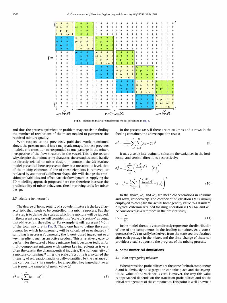

1500 D. Ponomarev et al. / Chemical Engineering and Processing 48 (2009) 1495–1505

ed to

atr

amiwbmors2pd

2

afiItopskpmoaitt

�

Fig. 6. Transition matrix relat

nd thus the process optimization problem may consist in findinghe number of revolutions of the mixer needed to guarantee theequired mixture quality.

With respect to the previously published work mentionedbove, the present model has a major advantage. In these previousodels, one transition corresponded to one passage in the mixer,

rrespective of the flow structure in the vessel. This is the reasonhy, despite their pioneering character, these studies could hardly

e directly related to mixer design. In contrast, the 2D Markovodel presented here represents flow at a mesoscopic level, that

f the mixing elements. If one of these elements is removed, oreplaced by another of a different shape, this will change the tran-ition probabilities and affect particle flow dynamics. Applying theD modelling approach proposed here can therefore increase theredictability of mixer behaviour, thus improving tools for mixeresign.

.3. Mixture homogeneity

The degree of homogeneity of a powder mixture is the key char-cteristic that needs to be controlled in a mixing process. But therst step is to define the scale at which the mixture will be judged.

n the present case, we will consider this “scale of scrutiny” as beinghat of the cells in the collector. For example, it will represent 1/40thf the total mixture in Fig. 3. Then, one has to define the com-onent for which homogeneity will be calculated or evaluated (ifampling is necessary), generally the lowest-dosed ingredient or aey ingredient such as an active product. This is relatively easy toerform for the case of a binary mixture, but it becomes tedious forulti-component mixtures with various key ingredients as is very

ften the case in the pharmaceutical industry. The homogeneity ofmixture containing N times the scale of scrutiny is also called the

ntensity of segregation and is usually quantified by the variance ofhe composition ci in sample i, for a specified key ingredient, over

he N possible samples of mean value 〈c〉:

2 = 1N

N∑i=1

(ci − 〈c〉)2 (8)

the model presented in Fig. 5.

In the present case, if there are m columns and n rows in thefeeding container, the above equation reads:

�2 = 1m · n

n∑i=1

m∑j=1

(cij − 〈c〉)2 (9)

It may also be interesting to calculate the variances in the hori-zontal and vertical directions, respectively:

�2x = 1

m

m∑j=1

(∑ni=1cij

n−⟨

cj

⟩)2

or �2z = 1

n

n∑i=1

(∑mj=1cij

m−⟨

ci

⟩)2

(10)

In the above, 〈cj〉 and 〈ci〉 are mean concentrations in columnsand rows, respectively. The coefficient of variation CV is usuallyemployed to compare the actual homogeneity value to a standard.A typical criterion retained for drug liberation is CV < 6%, and willbe considered as a reference in the present study:

CV = �〈c〉 (11)

In the model, the state vector directly represents the distributionof one of the components in the feeding container. As a conse-quence, the CV can easily be derived from the state vectors obtainedafter each passage in the mixer, and the time-change of these canprovide a visual support to the progress of the mixing process.

3. Some numerical simulations

3.1. Non-segregating mixtures

When transition probabilities are the same for both componentsA and B, obviously no segregation can take place and the asymp-totical value of the variance is zero. However, the way this valueis approached depends on the transition probabilities and on theinitial arrangement of the components. This point is well known in

D. Ponomarev et al. / Chemical Engineering and Processing 48 (2009) 1495–1505 1501

Fig. 7. State vector obtained for ps = 0.1 and pc = 0.3 (a, initial distribution; b, distribution after one pass; c, distribution after 10 passes).

F nts (ps = 0.1; pc = 0.3) as a function of the initial arrangement (vertical, a; horizontal, b).

im

tflstpmneFihdmtduch

tewcoa

brtt

ig. 8. Kinetics of binary mixing simulated with equal probabilities of the compone

ndustrial practice, but has never been taken into account in a flowodel for powders.Fig. 7 shows the distribution of the material in the loading con-

ainer after one pass in the mixing zone, as well as after 10 passes,or a vertical initial arrangement of the components, and for the fol-owing transition values: psA = psB = 0.1, pcA = pCB = 0.3. This diagramhows a concentration distribution among the cells in two direc-ions and gives a visual illustration of the progress of the mixingrocess. The surface is horizontal and all sections are filled to theaximum because the probabilities for A and B are equal. We can

ote that the mixture is almost homogeneous at the scale consid-red (1/120th of the total mixture) after 10 mixer revolutions only.ig. 8a shows the time-evolution of the variance for this verticalnitial arrangement and allows the results to be compared with aorizontal initial distribution (Fig. 8b). Both curves monotonouslyecrease with the increase in the number of revolutions of theixer, illustrating the absence of segregation phenomena. When

he components are placed in two horizontal layers, the varianceecreases more rapidly than in the case of the vertical config-ration. For example, after two rotations, for the probabilitiesonsidered, the values of the variance are 0.06 and 0.075 for theorizontal and vertical cases, respectively.

To better illustrate this idea, a brief analysis was performed toest the sensitivity of the model to its parameters in the case ofqual transition probabilities of the components. For this purpose,e considered a target homogeneity of CV = 6% and tried to find the

ombination of transition probabilities that allowed this value to bebtained. The results are reported in Fig. 9a (vertical arrangement)nd Fig. 9b (horizontal arrangement).

In the vertical arrangement, low values of pc are to be coupledy very high values of ps to give an acceptable homogeneity in aeasonable number of passes. In other words, a deficit in horizon-al mobility must be compensated by the same characteristics inhe vertical direction to prevent plug flow behaviour. For pc values

Fig. 9. Possible combinations of transition probabilities to reach a target value of6% on the CV of the mixtures, as a function of the initial arrangement (vertical, a;horizontal, b). Both components have same transition probabilities.

1502 D. Ponomarev et al. / Chemical Engineering and Processing 48 (2009) 1495–1505

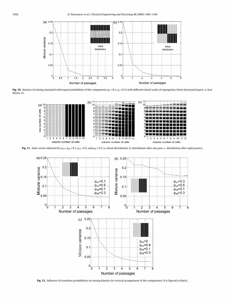
Fig. 10. Kinetics of mixing simulated with equal probabilities of the components (ps = 0.1; pc = 0.3) with different initial scales of segregation (three horizontal layers, a; fourblocks, b).

Fig. 11. State vector obtained for psA = psB = 0.1, pcA = 0.5, and psB = 0.3 (a, initial distribution; b, distribution after one pass; c, distribution after eight passes).

Fig. 12. Influence of transition probabilities on mixing kinetics for vertical arrangement of the components (A is figured in black).

D. Ponomarev et al. / Chemical Engineering and Processing 48 (2009) 1495–1505 1503

for ho

avtstfiebtwc

Fb

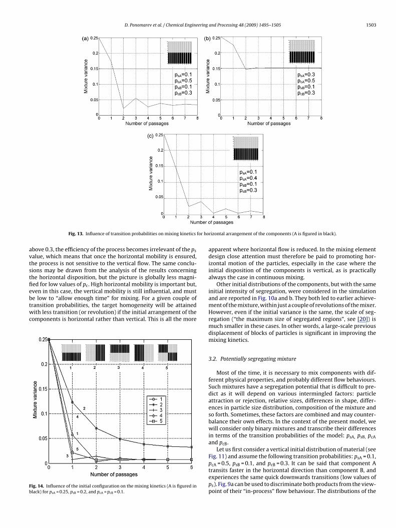
Fig. 13. Influence of transition probabilities on mixing kinetics

bove 0.3, the efficiency of the process becomes irrelevant of the ps

alue, which means that once the horizontal mobility is ensured,he process is not sensitive to the vertical flow. The same conclu-ions may be drawn from the analysis of the results concerninghe horizontal disposition, but the picture is globally less magni-ed for low values of pc. High horizontal mobility is important but,ven in this case, the vertical mobility is still influential, and must

e low to “allow enough time” for mixing. For a given couple ofransition probabilities, the target homogeneity will be attainedith less transition (or revolution) if the initial arrangement of the

omponents is horizontal rather than vertical. This is all the more

ig. 14. Influence of the initial configuration on the mixing kinetics (A is figured inlack) for psA = 0.25, psB = 0.2, and pcA = pcB = 0.1.

rizontal arrangement of the components (A is figured in black).

apparent where horizontal flow is reduced. In the mixing elementdesign close attention must therefore be paid to promoting hor-izontal motion of the particles, especially in the case where theinitial disposition of the components is vertical, as is practicallyalways the case in continuous mixing.

Other initial distributions of the components, but with the sameinitial intensity of segregation, were considered in the simulationand are reported in Fig. 10a and b. They both led to earlier achieve-ment of the mixture, within just a couple of revolutions of the mixer.However, even if the initial variance is the same, the scale of seg-regation (“the maximum size of segregated regions”, see [20]) ismuch smaller in these cases. In other words, a large-scale previousdisplacement of blocks of particles is significant in improving themixing kinetics.

3.2. Potentially segregating mixture

Most of the time, it is necessary to mix components with dif-ferent physical properties, and probably different flow behaviours.Such mixtures have a segregation potential that is difficult to pre-dict as it will depend on various intermingled factors: particleattraction or rejection, relative sizes, differences in shape, differ-ences in particle size distribution, composition of the mixture andso forth. Sometimes, these factors are combined and may counter-balance their own effects. In the context of the present model, wewill consider only binary mixtures and transcribe their differencesin terms of the transition probabilities of the model: psA, psB, pcAand pcB.

Let us first consider a vertical initial distribution of material (seeFig. 11) and assume the following transition probabilities: psA = 0.1,

pcA = 0.5, psB = 0.1, and pcB = 0.3. It can be said that component Atransits faster in the horizontal direction than component B, andexperiences the same quick downwards transitions (low values ofps). Fig. 9a can be used to discriminate both products from the view-point of their “in-process” flow behaviour. The distributions of the

1504 D. Ponomarev et al. / Chemical Engineering and Processing 48 (2009) 1495–1505

tics ob

cgtrzv

iptbi(wwindmdcettitkttliip

tpaimdpaIip

tmr

Fig. 15. Model and experimental data comparison for the mixing kine

omponents after one and eight passes are also given in the dia-rams representing the filling process of the cells. They show thathe free surface is actually irregular, due to preferential filling of theight part of the container. This is the result of the different hori-ontal transition probabilities that favour the retention of A in theessel.

Fig. 12a–c illustrates the influence of the transition probabil-ty values on the mixing kinetics by changing alternatively ps orc for one of the two components in the case of the initial ver-ical disposition. A small decrease in the vertical transitions of Ay changing ps from 0.1 to 0.3 leads to a serious slowing down

n the process, as well as some oscillations in the variance graphcompare Fig. 12a and b). The mixing kinetics is also improvedhen pcA is reduced from 0.5 to 0.4 (compare Fig. 12a and c),hich is closer to pcB. This behaviour cannot be explained by the

ntrinsic horizontal or vertical mobility values as is the case for theon-segregating mixtures. It is more likely to be the result of theifferences in transition probabilities between A and B. Indeed, theixing process is less efficient when the probabilities grow more

istant from each other. Fig. 13a–c shows the same ideas in thease of the horizontal arrangement to that concerning the influ-nce of the changing transition probabilities. The differences inhe transition probabilities of the two components clearly governhe mixing process. In addition, we can examine the effect of thenitial arrangement. As in the non-segregating case, the horizon-al disposition improves the mixture quality in terms of mixinginetics and “final” homogeneity. For example, it is 3–4 times bet-er in terms of variances after two passes in the system than forhe previous case. It must also be noted that clearly marked oscil-ations are now taking place, which must be taken into accountn process optimization. In particular, in Fig. 13a, mixture qual-ty is much better after two passes in the mixer than after eightasses.

Fig. 14 shows how the mixing kinetics is influenced by the ini-ial distribution of the components. The probabilities are psA = 0.25,sB = 0.2, and pcA = pcB = 0.1, so that a slight difference exists in thexial or crosswise mobility of particles, component A being retainedn the system more than component B. It can be seen that the best

ixture quality with the smallest mixing time is reached for theistribution in which the component having the higher downwardrobability (B) is placed at the top of the loading container. Oncegain, oscillations take place in the case of horizontal arrangements.t is somewhat remarkable to observe that even a decrease in thenitial scale of segregation (curve 5) does not lead to a better mixing

rocess.

All these examples of simulations serve to illustrate the sensi-ivity – in terms of both mixing kinetics and mixing time – of the

ixing process to the initial disposition of the component and theelative values of the transition probabilities. Particular attention

tained in the Sysmix® mixer with (a) or without (b) mixing elements.

must be paid to these factors if there is a potential risk of segregationof the particles.

4. Modelling of the Sysmix® mixer

To try to validate partially the Markov chain model developedin this work, we have used experimental data obtained and pub-lished by Gyenis and Arva in the studies we referred to previously.The authors considered two couples of components in their work,namely quartz–sodium chloride and flour–polypropylene granules,but we will focus only on the first couple. The initial arrangementof the components in the loading container was horizontal andorganized in three layers. During the mixing process, the mixerwas alternately revolved around the horizontal shaft at the mid-dle height of the mixing zone. The duration of a 180◦ rotation was1.5 s followed by a standstill of 3.0 s. With different mean particlesizes and densities, the components seemed to segregate duringthe experiments.

Transition probabilities were matched to the experimental databy minimizing difference between calculated and experimentalconcentrations in each column of the unloading container at everypass. Fig. 15 reports experimental data and adjusted model resultsfor the Sysmix® mixer with (a) or without (b) mixing elementsinserted. The best match was obtained for the following values ofthe transition probabilities:

- psA = 0.02, psB = 0.3, pcA = pcB = 0.1 with mixing elements.- psA = 0.01, psB = 0.12, pcA = pcB = 0.05 without mixing element.

The matching result is visually acceptable, which gives a positiveimpression about the ability of the model to calculate a real case.Some oscillations are found when mixing elements are inserted,but are due to the fact that the transition probability values arecloser in this case. This leads us again to conclude that segregationis not only caused by the intrinsic properties of the particles, but isalso due to their behaviour in a specific process. As might be imag-ined, the presence of the mixing elements in the mixer increasesthe horizontal mobility of the particles, as well as increasing theirretention in the system. It helps the mixing kinetics by inducing aquicker decrease in the variance of the mixture, but it also seemsthat variances are close to each other when the number of passesexceeds 6. It is therefore probable that the process is not yet opti-mized from the viewpoint of mixing element design. The presentmodel could be a very valuable tool for this task.

5. Conclusion

A two-dimensional model of particulate solid mixing was devel-oped on the basis of Markov chain theory. The prototype was the

ering

Sdtqoprtnm

-

-

-

-

A

Ccc

〈i

kmNPPPppp

p

pp

[

[

[

[

[

[

[

[

[

[

128–137.[20] P.V. Danckwerts, Theory of mixtures and mixing, Research (London) 6 (1953)

D. Ponomarev et al. / Chemical Engine

ysmix® mixer where mixing occurs both in vertical and horizontalirections. The model proposed makes it possible to calculate dis-ribution of components in two directions and to estimate mixtureuality accurately. Simulations were run to investigate the effectf initial material loading and to analyse the effect of transitionrobability values on the mixing kinetics, so as to take particle seg-egation into account. It was shown that while mixing componentshat tend to segregate, there is a rational way of loading compo-ents, and an optimal number of revolutions giving the maximalixture quality.Main issues for improving the current model are:

Linking transition probabilities to particle flow characteristics ina definite process configuration. This could be done experimen-tally, but also through the help of other models, like DEM at thelevel of a cell, for example. This could therefore give rise to ahybrid model of flow in static mixers.Validation of the model by new sets of experiments, testing effec-tively the effects of different process variables on the transitionprobabilities, and refining the approach by identifying process-dependent parameters and product-dependent parameters.Optimization of the design and operation of static mixers (num-ber, shape, spatial disposition, type of mixing elements) by usingthe model. In other words, finding the best combination oftransition probabilities and relating this to mixing element char-acteristics. This constitutes a real technological challenge.Considering more realistic features for the Markov model, such astime- or state-dependent transition matrices, or interdependenttransition probabilities such as in [21]. The way transition prob-abilities for a component are affected by the presence of anothercomponent of different transition probabilities is still difficult toapprehend.

ppendix A. List of symbols

V coefficient of variation of a mixturei key component content in sample number i

ij content in sample corresponding to the position i, j in thecontainer

c〉 key component mean content in samples, j indexes for matrix elements or for location of samples in

the containerindex for transition number

, n indexes for matrix dimensionnumber of samplestransition matrix

A, PB transition matrices for component A and Bij block matrixij element of Pc transition probability (horizontal)cA, pcB transition probabilities (horizontal) for component A and

BsA, psB transition probabilities (staying in a cell) for component

A and Bd transition probability (downwards)s transition probability (staying in a cell)

[

and Processing 48 (2009) 1495–1505 1505

S state vectorS(k)

ffeed state vector at transition k

Sm state matrixsi element of Sm

sij element of SZ zero block matrix� mixture standard deviation�x mixture standard deviation in horizontal direction�z mixture standard deviation in vertical direction

References

[1] M. Moakher, T. Shinbrot, F.J. Muzzio, Experimentally validated computations offlow, mixing and segregation of non-cohesive grains in 3D tumbling blenders,Powder Technology 109 (2000) 58–71.

[2] J.J. Mc Carthy, J.M. Ottino, Particle dynamics simulation: a hybrid techniqueapplied to granular mixing, Powder Technology 97 (1998) 91–99.

[3] J. Doucet, N. Hudon, F. Bertrand, C. Chaouki, Modeling of the mixing of monodis-perse particles using a stationary DEM-based Markov process, Computers &Chemical Engineering 32 (6) (2008) 1334–1341.

[4] S.J. Chen, L.T. Fan, C.A. Watson, The mixing of solids particles in a motionlessmixer—a stochastic approach, AIChE Journal 18 (5) (1972) 984–989.

[5] R.H. Wang, L.T. Fan, Axial mixing of grains in a motionless Sulzer (Koch) mixer,Industrial & Engineering Chemistry: Process Design & Development 15 (3)(1976) 381–388.

[6] R.H. Wang, L.T. Fan, Stochastic modelling of segregation in a motionless mixer,Chemical Engineering Science 32 (1977) 695–701.

[7] R.O. Fox, L.T. Fan, Stochastic analysis of axial solids mixing in a fluidized bed, in:1st World Congress on Particle Technology, vol. III, Nuremberg, 1986, p. 581.

[8] H.G. Dehling, A.C. Hoffman, H.W. Stuut, Stochastic models for transport in afluidised bed, SIAM Journal of Applied Mathematics 60 (1) (1999) 337–358.

[9] L.T. Fan, S.H. Shin, Stochastic diffusion model of non-ideal mixing in a horizontaldrum mixer, Chemical Engineering Science 34 (1979) 811–820.

10] M. Aoun Habbache, M. Aoun, H. Berthiaux, V. Mizonov, An experimentalmethod and a Markov chain model to describe axial and radial mixing in ahoop mixer, Powder Technology 128 (2002) 150–167.

11] K. Marikh, H. Berthiaux, V. Mizonov, E. Barantseva, D. Ponomarev, Flow analysisand Markov chain modelling to quantify the agitation effect in a continuouspowder mixer, Chemical Engineering Research and Design, Transactions of theIChemE Part A 84 (A11) (2006) 1059–1074.

12] D Ponomarev, C. Gatumel, V. Mizonov, H. Berthiaux, E. Barantseva, Markovchain modelling and experimental investigation of mixing kinetics in staticrevolving powder mixers, Chemical Engineering and Processing: Process Inten-sification 48 (3) (2009) 828–836.

13] J. Gyenis, J. Arva, Mixing mechanism of solids in alternately revolving mixers,I, Powder Handling & Processing 1 (3) (1989) 247–254.

14] J. Gyenis, J. Arva, Improvement of mixing rate of solids by motionless mixergrids in alternately revolving mixers, Powder Handling & Processing 1 (2)(1989) 165–171.

15] J. Gyenis, F. Katai, Determination and randomness in mixing of particulatesolids, Chemical Engineering Science 45 (9) (1990) 2843–2855.

16] J. Gyenis, J. Arva, J. Nemeth, Mixing and demixing of non ideal solid particlesystems in alternating batch mixer, Hungarian Journal of Industrial Chemistry19 (1) (1991) 69–74.

17] H. Berthiaux, V. Mizonov, Application of Markov chains in particulate processengineering: a review, The Canadian Journal of Chemical Engineering 82 (6)(2004) 1143–1168.

18] V. Mizonov, H. Berthiaux, V. Zhukov, S. Bernotat, Application of multi-dimensional Markov chains to model kinetics of grinding with internalclassification, International Journal of Mineral Processing 74 (1001) (2004)307–315.

19] H. Berthiaux, V. Mizonov, Application of the theory of Markov chains to modeldifferent processes in particle technology, Powder Technology 157 (2005)

355–361.21] C.H. Chou, J.R. Johnson, E.G. Rippie, Polydisperse particulate solids mixing and

segregation: nonstationary Markov chains, Journal of Pharmaceutical Sciences66 (1) (1977) 104–106.