arX

iv:1

003.

0052

v1 [

astr

o-ph

.SR

] 2

7 Fe

b 20

10accepted by ApJPreprint typeset using LATEX style emulateapj v. 11/10/09

A MULTI-SITE CAMPAIGN TO MEASURE SOLAR-LIKE OSCILLATIONS IN PROCYON.II. MODE FREQUENCIES

Timothy R. Bedding,1 Hans Kjeldsen,2 Tiago L. Campante,2,3 Thierry Appourchaux,4 Alfio Bonanno,5

William J. Chaplin,6 Rafael A. Garcia,7 Milena Martic,8 Benoit Mosser,9 R. Paul Butler,10 Hans Bruntt,1,11

Laszlo L. Kiss,1,12 Simon J. O’Toole,13 Eiji Kambe,14 Hiroyasu Ando,15 Hideyuki Izumiura,14 Bun’ei Sato,16

Michael Hartmann,17 Artie Hatzes,17 Caroline Barban,11 Gabrielle Berthomieu,18 Eric Michel,11

Janine Provost,18 Sylvaine Turck-Chieze,7 Jean-Claude Lebrun,8 Jerome Schmitt,19 Jean-Loup Bertaux,8

Serena Benatti,20 Riccardo U. Claudi,21 Rosario Cosentino,5 Silvio Leccia,22 Søren Frandsen,2

Karsten Brogaard,2 Lars Glowienka,2 Frank Grundahl,2 Eric Stempels,23 Torben Arentoft,2

Michael Bazot,2 Jørgen Christensen-Dalsgaard,2 Thomas H. Dall,24 Christoffer Karoff,2

Jens Lundgreen-Nielsen,2 Fabien Carrier,25 Patrick Eggenberger,26 Danuta Sosnowska,27

Robert A. Wittenmyer,28,29 Michael Endl,28 Travis S. Metcalfe,30 Saskia Hekker,6,31 and Sabine Reffert32

accepted by ApJ

ABSTRACT

We have analyzed data from a multi-site campaign to observe oscillations in the F5 star Procyon. The data consistof high-precision velocities that we obtained over more than three weeks with eleven telescopes. A new method foradjusting the data weights allows us to suppress the sidelobes in the power spectrum. Stacking the power spectrumin a so-called echelle diagram reveals two clear ridges that we identify with even and odd values of the angular degree(l = 0 and 2, and l = 1 and 3, respectively). We interpret a strong, narrow peak at 446µHz that lies close to thel = 1 ridge as a mode with mixed character. We show that the frequencies of the ridge centroids and their separationsare useful diagnostics for asteroseismology. In particular, variations in the large separation appear to indicate a glitchin the sound-speed profile at an acoustic depth of ∼1000 s. We list frequencies for 55 modes extracted from thedata spanning 20 radial orders, a range comparable to the best solar data, which will provide valuable constraintsfor theoretical models. A preliminary comparison with published models shows that the offset between observed andcalculated frequencies for the radial modes is very different for Procyon than for the Sun and other cool stars. We findthe mean lifetime of the modes in Procyon to be 1.29+0.55

−0.49 days, which is significantly shorter than the 2–4 days seenin the Sun.

Subject headings: stars: individual (Procyon A) — stars: oscillations

1 Sydney Institute for Astronomy (SIfA), School ofPhysics, University of Sydney, NSW 2006, Australia; bed-ding@physics.usyd.edu.au

2 Danish AsteroSeismology Centre (DASC), Department ofPhysics and Astronomy, Aarhus University, DK-8000 Aarhus C,Denmark

3 Centro de Astrofısica da Universidade do Porto, Rua dasEstrelas, 4150-762 Porto, Portugal

4 Institut d’Astrophysique Spatiale, Universite Paris XI-CNRS,Batiment 121, 91405 Orsay Cedex, France

5 INAF – Osservatorio Astrofisico di Catania, via S. Sofia 78,95123 Catania, Italy

6 School of Physics and Astronomy, University of Birmingham,Edgbaston, Birmingham B15 2TT, UK

7 DAPNIA/DSM/Service d’Astrophysique, CEA/Saclay, 91191Gif-sur-Yvette Cedex, France

8 LATMOS, University of Versailles St Quentin, CNRS, BP 3,91371 Verrieres le Buisson Cedex, France

9 LESIA, CNRS, Universite Pierre et Marie Curie, UniversiteDenis Diderot, Observatoire de Paris, 92195 Meudon cedex, France

10 Carnegie Institution of Washington, Department of Terres-trial Magnetism, 5241 Broad Branch Road NW, Washington, DC20015-1305

11 Laboratoire AIM, CEA/DSM – CNRS - Universite ParisDiderot – IRFU/SAp, 91191 Gif-sur-Yvette Cedex, France

12 Konkoly Observatory of the Hungarian Academy of Sciences,H-1525 Budapest, P.O. Box 67, Hungary

13 Anglo-Australian Observatory, P.O.Box 296, Epping, NSW1710, Australia

14 Okayama Astrophysical Observatory, National AstronomicalObservatory of Japan, National Institutes of Natural Sciences,3037-5 Honjyo, Kamogata, Asakuchi, Okayama 719-0232, Japan

15 National Astronomical Observatory of Japan, National Insti-tutes of Natural Sciences, 2-21-1 Osawa, Mitaka, Tokyo 181-8588,Japan

16 Global Edge Institute, Tokyo Institute of Technology 2-12-1-S6-6, Ookayama, Meguro-ku, Tokyo 152-8550, Japan

17 Thuringer Landessternwarte Tautenburg, Sternwarte 5, 07778Tautenburg, Germany

18 Universite de Nice Sophia-Antipolis, CNRS UMR 6202,Laboratoire Cassiopee, Observatoire de la Cote d’Azur, BP 4229,06304 Nice Cedex, France

19 Observatoire de Haute Provence, 04870 St Michell’Observatoire, France

20 CISAS – University of Padova, Via Venezia 5, 35131, Padova,Italy

21 INAF – Astronomical Observatory of Padua, Vicolo Osserva-torio 5, 35122 Padova, Italy

22 INAF – Osservatorio Astronomico di Capodimonte, SalitaMoiariello 16, 80131 Napoli, Italy

23 Department of Physics and Astronomy, Box 516, SE-751 20Uppsala, Sweden

24 European Southern Observatory, D-85748 Garching, Ger-many

25 Instituut voor Sterrenkunde, Katholieke Universiteit Leuven,Celestijnenlaan 200 B, 3001 Leuven, Belgium

26 Observatoire de Geneve, Universite de Geneve, Ch. desMaillettes 51, CH-1290 Sauverny, Switzerland

27 Laboratoire d’astrophysique, EPFL Observatoire CH-1290Versoix

28 McDonald Observatory, University of Texas at Austin,Austin, TX 78712, USA

29 School of Physics, University of New South Wales, NSW2052, Australia

30 High Altitude Observatory, National Centre for AtmosphericResearch, Boulder, CO 80307-3000 USA

31 Leiden Observatory, Leiden University, 2300 RA Leiden, TheNetherlands

32 ZAH-Landessternwarte, 69117 Heidelberg, Germany

2 Bedding et al.

1. INTRODUCTION

The success of helioseismology and the promise ofasteroseismology have motivated numerous efforts tomeasure oscillations in solar-type stars. These beganwith ground-based observations (for recent reviews seeBedding & Kjeldsen 2007; Aerts et al. 2008) and now ex-tend to space-based photometry, particularly with theCoRoT and Kepler Missions (e.g., Michel et al. 2008;Gilliland et al. 2010).We have carried out a multi-site spectroscopic cam-

paign to measure oscillations in the F5 star Procyon A(HR 2943; HD 61421; HIP 37279). We obtained high-precision velocity observations over more than threeweeks with eleven telescopes, with almost continu-ous coverage for the central ten days. In Paper I(Arentoft et al. 2008) we described the details of the ob-servations and data reduction, measured the mean oscil-lation amplitudes, gave a crude estimate for the modelifetime and discussed slow variations in the velocitycurve that we attributed to rotational modulation of ac-tive regions. In this paper we describe the procedureused to extract the mode parameters, provide a list ofoscillation frequencies, and give an improved estimate ofthe mode lifetimes.

2. PROPERTIES OF SOLAR-LIKE OSCILLATIONS

We begin with a brief summary of the relevant prop-erties of solar-like oscillations (for reviews see, for exam-ple, Brown & Gilliland 1994; Bedding & Kjeldsen 2003;Christensen-Dalsgaard 2004).To a good approximation, in main-sequence stars

the cyclic frequencies of low-degree p-mode oscillationsare regularly spaced, following the asymptotic relation(Tassoul 1980; Gough 1986):

νn,l ≈ ∆ν(n+ 12 l+ ǫ)− l(l+ 1)D0. (1)

Here n (the radial order) and l (the angular degree) areintegers, ∆ν (the large separation) depends on the soundtravel time across the whole star, D0 is sensitive to thesound speed near the core and ǫ is sensitive to the reflec-tion properties of the surface layers. It is conventionalto define three so-called small frequency separations thatare sensitive to the sound speed in the core: δν02 is thespacing between adjacent modes with l = 0 and l = 2(for which n will differ by 1); δν13 is the spacing betweenadjacent modes with l = 1 and l = 3 (ditto); and δν01is the amount by which l = 1 modes are offset from themidpoint of the l = 0 modes on either side.33 To be ex-plicit, for a given radial order, n, these separations aredefined as follows:

δν02= νn,0 − νn−1,2 (2)

δν01=12 (νn,0 + νn+1,0)− νn,1 (3)

δν13= νn,1 − νn−1,3. (4)

If the asymptotic relation (equation 1) were to hold ex-actly, it would follow that all of these separations wouldbe independent of n and that δν02 = 6D0, δν13 = 10D0

and δν01 = 2D0. In practice, equation (1) is only an

33 One can also define an equivalent quantity, δν10, as the offsetof l = 0 modes from the midpoint between the surrounding l = 1modes, so that δν10 = νn,0 − 1

2(νn−1,1 + νn,1).

approximation. In the Sun and other stars, theoreticalmodels and observations show that ∆ν, D0 and ǫ varysomewhat with frequency, and also with l. Consequently,the small separations also vary with frequency.The mode amplitudes are determined by the excita-

tion and damping, which are stochastic processes involv-ing near-surface convection. We typically observe modesover a range of frequencies, which in Procyon is especiallybroad (about 400–1400µHz; see Paper I). The observedamplitudes also depend on l via various projection factors(see Table 1 of Kjeldsen et al. 2008a). Note in particularthat velocity measurements are much more sensitive tomodes with l = 3 than are intensity measurements. Themean mode amplitudes are modified for a given observ-ing run by the stochastic nature of the excitation, result-ing in considerable scatter of the peak heights about theenvelope.Oscillations in the Sun are long-lived compared to their

periods, which allows their frequencies to be measuredvery precisely. However, the lifetime is not infinite andthe damping results in each mode in the power spectrumbeing split into multiple peaks under a Lorentzian profile.The FWHM of this Lorentzian, which is referred to asthe linewidth Γ, is inversely proportional to the modelifetime: Γ = 1/(πτ). We follow the usual definition thatτ is the time for the mode amplitude to decay by a factorof e. The solar value of τ for the strongest modes rangesfrom 2 to 4 days, as a decreasing function of frequency(e.g., Chaplin et al. 1997).Procyon is an evolved star, with theoretical mod-

els showing that it is close to, or just past, the endof the main sequence (e.g., Guenther & Demarque1993; Barban et al. 1999; Chaboyer et al. 1999;Di Mauro & Christensen-Dalsgaard 2001; Kervella et al.2004; Eggenberger et al. 2005; Provost et al. 2006;Bonanno et al. 2007; Guenther et al. 2008). As such,its oscillation spectrum may show deviations from theregular comb-like structure described by equation (1),especially at low frequencies. This is because somemodes, particularly those with l = 1, are shifted byavoided crossings with gravity modes in the stellarcore (also called ‘mode bumping’; see Osaki 1975;Aizenman et al. 1977). These so-called ‘mixed modes’have p-mode character near the surface but g-modecharacter in the deep interior. Some of the theoreticalmodels of Procyon cited above indeed predict thesemixed modes, depending on the evolutionary state of thestar, and we must keep this in mind when attempting toidentify oscillation modes in the power spectrum. Themixed modes are rich in information because they probethe stellar core and are very sensitive to age, but theycomplicate the task of mode identification.We should also keep in mind that mixed modes are

expected to have lower amplitudes and longer lifetimes(smaller linewidths) than regular p modes because theyhave larger mode inertias (e.g., Christensen-Dalsgaard2004). Hence, for a data series that is many times longerthan the lifetime of the pure p modes, a mixed mode mayappear in the power spectrum as a narrow peak that ishigher than the others, even though its power (amplitudesquared) is not especially large.Another potential complication is that stellar rota-

tion causes modes with l ≥ 1 to split into multiplets.The peaks of these multiplets are characterized by the

Oscillations in Procyon. II. Frequencies 3

azimuthal degree m, which takes on values of m =0,±1, . . . ,±l, with a separation that directly measuresthe rotation rate averaged over the region of the star thatis sampled by the mode. The measurements are particu-larly difficult because a long time series is needed to re-solve the rotational splittings. We argue in Appendix Athat the low value of v sin i observed in Procyon impliesthat rotational splitting of frequencies is not measurablein our observations.

3. WEIGHTING THE TIME SERIES

The time series of velocity observations was obtainedover 25 days using 11 telescopes at eight observatoriesand contains just over 22 500 data points. As discussed inPaper I, the velocity curve shows slow variations that weattribute to a combination of instrumental drifts and ro-tational modulation of stellar active regions. We have re-moved these slow variations by subtracting all the powerbelow 280µHz, to prevent spectral leakage into higherfrequencies that would degrade the oscillation spectrum.We take this high-pass-filtered time series of velocities,together with their associated measurement uncertain-ties, as the starting point in our analysis.

3.1. Noise-optimized weights

Using weights when analyzing ground-based observa-tions of stellar oscillations (e.g., Gilliland et al. 1993;Frandsen et al. 1995) allows one to take into account thesignificant variations in data quality during a typical ob-serving campaign, especially when two or more telescopesare used. The usual practice, which we followed in Pa-per I, is to calculate the weights for a time series from themeasurement uncertainties, σi, according to wi = 1/σ2

i .These “raw” weights can then be adjusted to minimize

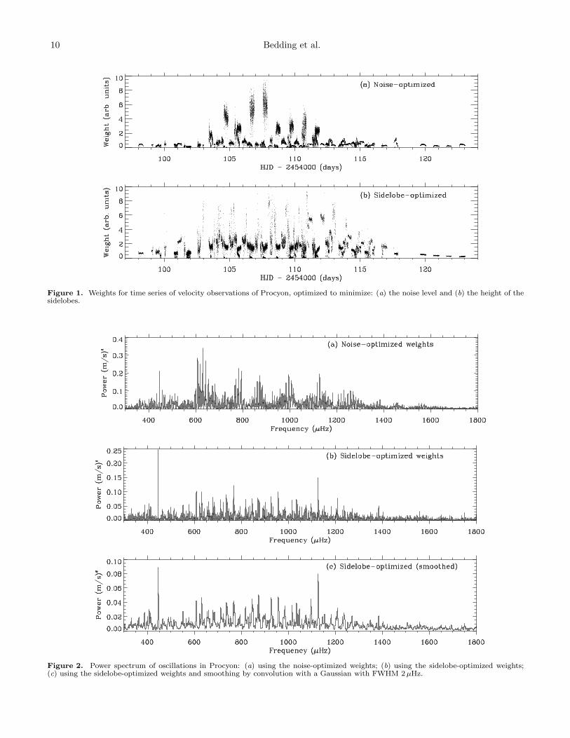
the noise level in the final power spectrum by identifyingand revising those uncertainties that are too optimistic,and at the same time rescaling the uncertainties to bein agreement with the actual noise levels in the data.This procedure is described in Paper I and referencestherein. The time series of these noise-optimized weightsis shown in Figure 1a. These are the same as those shownin Figure 1d of Paper I, but this time as weights ratherthan uncertainties.The power spectrum of Procyon based on these noise-

optimized weights is shown in Figure 2a. This is the sameas shown in Paper I (lower panel of Figure 6), exceptthat the power at low frequencies, which arises from theslow variations, has been removed. As described in Pa-per I, the noise level above 3mHz in this noise-optimizedspectrum is 1.9 cm s−1 in amplitude. This includes somedegree of spectral leakage from the oscillations and if wehigh-pass filter the spectrum up to 3mHz to remove theoscillation signal, the noise level drops to 1.5 cm s−1 inamplitude.The task of extracting oscillation frequencies from the

power spectrum is complicated by the presence of struc-ture in the spectral window, which are caused by gaps orotherwise uneven coverage in the time series. The spec-tral window using the noise-optimized weights is shownin Figure 3a. Prominent sidelobes at ±11.57µHz cor-respond to aliasing at one cycle per day. Indeed, theprospect of reducing these sidelobes is the main reasonfor acquiring multi-site observations. However, even withgood coverage the velocity precision varies greatly, both

for a given telescope during the run and from one tele-scope to another (see Figure 1a). As pointed out in Pa-per I, using these measurement uncertainties as weightshas the effect of increasing the sidelobes in the spectralwindow. We now discuss a technique for addressing thisissue.

3.2. Sidelobe-optimized weights

Adjusting the weights allows one to suppress the side-lobe structure; the trade-off is an increase in the noiselevel. This technique is routinely used in radio astron-omy when synthesising images from interferometers (e.g.,Hogbom & Brouw 1974). An extreme case is to set allweights to be equal, which is the same as not usingweights at all. This is certainly not optimal because itproduces a power spectrum with greatly increased noise(by a factor of 2.3) but still having significant sidelobes,as can be seen in Figure 6a of Paper I. Adjusting theweights on a night-by-night basis in order to minimizethe sidelobes was used in the analysis of dual-site ob-servations of α Cen A (Bedding et al. 2004), α Cen B(Kjeldsen et al. 2005), and β Hyi (Bedding et al. 2007).For our multi-site Procyon data this is impractical be-cause of the large number of (partly overlapping) tele-scope nights. We have developed a more general algo-rithm for adjusting weights to minimize the sidelobes (H.Kjeldsen et al., in prep.). The new method, which is su-perior because it does not assume the oscillations arecoherent over the whole observing run, is based on theprinciple that equal weight is given to all segments of thetime series. The method produces the cleanest possiblespectral window in terms of suppressing the sidelobes,and we have tested it with good results using publisheddata for α Cen A and B, and β Hyi (Arentoft et al. 2010).The new method operates with two timescales, T1 and

T2. All data segments of length T1 (=2 hr, in this case)are required to have the same total weight throughout thetime series, with the relaxing condition that variationson time scales longer than T2 (=12hr) are retained. Tobe explicit, the algorithm works as follows. We adjustthe weights so that all segments of length T1 have thesame total weight. That is, for each point wi in the timeseries of weights, define {Si} to be the set of weightsin a segment of width T1 centered at that time stamp,and divide each wi by the sum of the weights in {Si}.However, this adjustment suffers from edge effects, sinceit gives undue weight to points adjacent to a gap. Tocompensate, we also divide by an asymmetry factor

R = 1 +

∣

∣

∣

∣

Σleft − Σright

Σleft +Σright

∣

∣

∣

∣

. (5)

Here, Σleft is the sum of the weights in the segment {Si}that have time stamps less than ti, and Σright is the sumof the weights in the segment {Si} that have time stampsgreater than ti. Note that R ranges from 1, for pointsthat are symmetrically placed in their T bin, up to 2 forpoints at one edge of a gap.Once the above procedure is done for T1, which is

the shortest timescale on which we wish to adjust theweights, we do it again with T2, which is the longesttimescale for adjusting the weights. Finally, we dividethe first set of adjusted weights by the second set, andthis gives the weights that we adopt (Figure 1b).

4 Bedding et al.

3.3. The sidelobe-optimized power spectrum

Figure 2b shows the power spectrum of Procyon basedon the sidelobe-optimized weights. The spectral windowhas improved tremendously (Figure 3b), while the noiselevel at high frequencies (above 3mHz) has increased bya factor of 2.0.The power spectrum now clearly shows a regular series

of peaks, which are even more obvious after smoothing(Figure 2c). We see that the large separation of the staris about 55µHz, confirming the value indicated by severalprevious studies (Mosser et al. 1998; Martic et al. 1999,2004; Eggenberger et al. 2004; Regulo & Roca Cortes2005; Leccia et al. 2007; Guenther et al. 2008). The verystrong peak at 446µHz appears to be a candidate for amixed mode, especially given its narrowness (see Sec-tion 2).Plotting the power spectrum in echelle format using a

large separation of 56µHz (Figure 4) clearly shows tworidges, as expected.34 The upper parts are vertical butthe lower parts are tilted, indicating a change in the largeseparation as a function of frequency. This large amountof curvature in the echelle diagram goes a long way to-wards explaining the lack of agreement between previousstudies on the mode frequencies of Procyon (see the listof references given in the previous paragraph).The advantage of using the sidelobe-optimized weights

is demonstrated by Figure 5. This is the same as Figure 4but for the noise-optimized weights and the ridges are nolonger clearly defined.

4. IDENTIFICATION OF THE RIDGES

We know from asymptotic theory (see equation 1) thatone of the ridges in the echelle diagram (Figure 4) cor-responds to modes with even degree (l = 0 and 2) andthe other to modes with odd degree (l = 1 and 3). How-ever, it is not immediately obvious which is which. Wealso need to keep in mind that the asymptotic relationin evolved stars does not hold exactly. We designatethe two possibilities Scenario A, in which the left-handridge in Figure 4 corresponds to modes with odd degree,and Scenario B, in which the same ridge corresponds tomodes with even degree. Figure 6 shows the Procyonpower spectrum collapsed along several orders. We seenow double peaks that suggest the identifications shown,which corresponds to Scenario B.We can check that the small separation δν01 has the

expected sign. According to asymptotic theory (equa-tion 1), each l = 1 mode should be at a slightly lower fre-quency than the mid-point of the adjacent l = 0 modes.This is indeed the case for the identifications given inFigure 6, but would not be if the even and odd degreeswere reversed. We should be careful, however, since δν01has been observed to have the opposite sign in red giantstars (Carrier et al. 2010; Bedding et al. 2010).The problem of ridge identification in F stars

was first encountered by Appourchaux et al. (2008)when analysing CoRoT observations of HD 49933

34 When making an echelle diagram, it is common to plot ν ver-sus (ν mod ∆ν), in which case each order slopes upwards slightly.However, for gray-scale images it is preferable to keep the ordershorizontal, as was done in the original presentation of the diagram(Grec et al. 1983). We have followed that approach in this paper,and the value given on the vertical axis indicates the frequency atthe middle of each order.

and has been followed up by numerous authors(Benomar et al. 2009a,b; Gruberbauer et al. 2009;Mosser & Appourchaux 2009; Roxburgh 2009;Kallinger et al. 2010). Two other F stars observedby CoRoT have presented the same problem, namelyHD 181906 (Garcıa et al. 2009) and HD 181420(Barban et al. 2009). A discussion of the issue wasrecently given by Bedding & Kjeldsen (2010), who pro-posed a solution to the problem that involves comparingtwo (or more) stars on a single echelle diagram afterfirst scaling their frequencies.Figure 7 shows the echelle diagram for Procyon

overlaid with scaled frequencies for two stars ob-served by CoRoT, using the method described byBedding & Kjeldsen (2010). The filled symbols arescaled oscillation frequencies for the G0 star HD 49385observed by CoRoT (Deheuvels et al. 2010). The scalinginvolved multiplying all frequencies by a factor of 0.993before plotting them, with this factor being chosen toalign the symbols as closely as possible with the Procyonridges. For this star the CoRoT data gave an unam-biguous mode identification, which is indicated by thesymbol shapes. This confirms that the left-hand ridge ofProcyon corresponds to modes with even l (Scenario B).The open symbols in Figure 7 are oscillation fre-

quencies for HD 49933 from the revised identifica-tion by Benomar et al. (2009b, Scenario B), after mul-tiplying by a scaling factor of 0.6565. The align-ment with HD 49385 was already demonstrated byBedding & Kjeldsen (2010). We show HD 49933 herefor comparison and to draw attention to the differentamounts of bending at the bottom of the right-hand(l = 1) ridge for the three stars. The CoRoT targetthat is most similar to Procyon is HD170987 but un-fortunately the S/N ratio is too low to provide a clearidentification of the ridges (Mathur et al. 2010).The above considerations give us confidence that Sce-

nario B in Procyon is the correct identification, and wenow proceed on that basis.

5. FREQUENCIES OF THE RIDGE CENTROIDS

Our next step in the analysis was to measure the cen-troids of the two ridges in the echelle diagram. Wefirst removed the strong peak at 446µHz (it was re-placed by the mean noise level). We believe this tobe a mixed mode and its extreme power means that itwould significantly distort the result. We then smoothedthe power spectrum to a resolution of 10µHz (FWHM).To further improve the visibility of the ridges, we alsoaveraged across several orders, which corresponds tosmoothing in the vertical direction in the echelle dia-gram (Bedding et al. 2004; Kjeldsen et al. 2005; Karoff2007). That is, for a given value of ∆ν we define the“order-averaged” power-spectrum to be

OAPS(ν,∆ν) =

4∑

j=−4

cjPS(ν + j∆ν). (6)

The coefficients cj are chosen to give a smoothing witha FWHM of k∆ν:

cj = c−j =1

1 + (2j/k)2. (7)

Oscillations in Procyon. II. Frequencies 5

We show in Figure 8 the OAPS based on smoothingover 4 orders (k = 4.0), and so we used (c0, . . . , c4) =(1, 0.8, 0.5, 0.31, 0.2). The OAPS is plotted for three val-ues of the large separations (54, 55 and 56µHz) and theyare superimposed. The three curves are hardly distin-guishable and we see that the positions of the maximaare not sensitive to the value of ∆ν.We next calculated a modified version of the OAPS

in which the value at each frequency is the maximumvalue of the OAPS over a range of large separations (53–57µHz). This is basically the same as the comb response,as used previously by several authors (Kjeldsen et al.1995; Mosser et al. 1998; Martic et al. 1999; Leccia et al.2007). The maxima of this function define the centroidsof the two ridges, which are shown in Figure 9.In Figure 10 we show the full power spectrum of Pro-

cyon (using sidelobe-optimized weights) collapsed alongthe ridges. This is similar to Figure 6 except that eachorder was shifted before the summation, so as to alignthe ridge peaks (symbols in Figure 9) and hence removethe curvature. This was done separately for both theeven- and odd-degree ridges, as shown in the two pan-els of Figure 10. The collapsed spectrum clearly showsthe power corresponding to l = 0–3, as well as the extrapower from the mixed modes (for this figure, the peak at446µHz has not been removed).In Section 6 below, we use the ridges to guide our

identification of the individual modes. First, however,we show that some asteroseismological inferences can bemade solely from the ridges themselves. This is explainedin more detail in Appendix B.

5.1. Large separation of the ridges

Figure 11a shows the variation with frequency of thelarge separation for each of the two ridges (diamondsand triangles). The smoothing across orders (equation 6)means that the ridge frequencies are correlated from oneorder to the next and so we used simulations to estimateuncertainties for the ridge centroids.The oscillatory behavior of ∆ν as a function of fre-

quency seen in Figure 11a is presumably a signature ofthe helium ionization zone (e.g. Gough 1990). The os-cillation is also seen in Figure 11b, which shows the sec-ond differences for the two ridges, defined as follows (seeGough 1990; Ballot et al. 2004; Houdek & Gough 2007):

∆2νn,even= νn−1,even − 2νn,even + νn+1,even (8)

∆2νn,odd= νn−1,odd − 2νn,odd + νn+1,odd. (9)

The period of the oscillation is ∼500µHz, which impliesa glitch at an acoustic depth that is approximately twicethe inverse of this value (Gough 1990; Houdek & Gough2007), namely ∼1000 s. To determine this more precisely,we calculated the power spectrum of the second differ-ences for both the odd and even ridges, and measuredthe highest peak. We found the period of the oscillationin the second differences to be 508± 18µHz. Comparingthis result with theoretical models will be the subject ofa future paper.The dotted lines in Figure 11a show the variation of ∆ν

with frequency calculated from the autocorrelation of thetime series using the method of Mosser & Appourchaux(2009, see also Roxburgh & Vorontsov 2006). The mixedmode at 446µHz was first removed and the smoothing

filter had FWHM equal to 3 times the mean large sepa-ration. We see general agreement with the values calcu-lated from the ridge separations. Some of the differencespresumably arise because the autocorrelation analysis ofthe time series averages the large separation over all de-grees.

5.2. Small separation of the ridges

Using only the centroids of the ridges, we can measurea small separation that is useful for asteroseismology. Byanalogy with δν01 (see equation 3), we define it as theamount by which the odd ridge is offset from the mid-point of the two adjacent even ridges, with a positivevalue corresponding to a leftwards shift (as observed inthe Sun). That is,

δνeven,odd =νn,even + νn+1,even

2− νn,odd. (10)

Figure 11c shows our measurements of this small sepa-ration.35 It is related in a simple way to the conven-tional small separations δν01, δν02, and δν13 (see Ap-pendix B for details) and so, like them, it gives infor-mation about the sound speed in the core. Our mea-surements of this small separation can be compared withtheoretical models using the equations in Appendix B(e.g., see Christensen-Dalsgaard & Houdek 2009).

6. FREQUENCIES OF INDIVIDUAL MODES

We have extracted oscillation frequencies from the timeseries using the standard procedure of iterative sine-wavefitting. Each step of the iteration involves finding thestrongest peak in the sidelobe-optimized power spectrumand subtracting the corresponding sinusoid from the timeseries. Figure 12 shows the result. The two ridges areclearly visible but the finite mode lifetime causes manymodes to be split into two or more peaks. We mightalso be tempted to propose that some of the multiplepeaks are due to rotational splitting but, as shown inAppendix A, this is unlikely to be the case.Deciding on a final list of mode frequencies with cor-

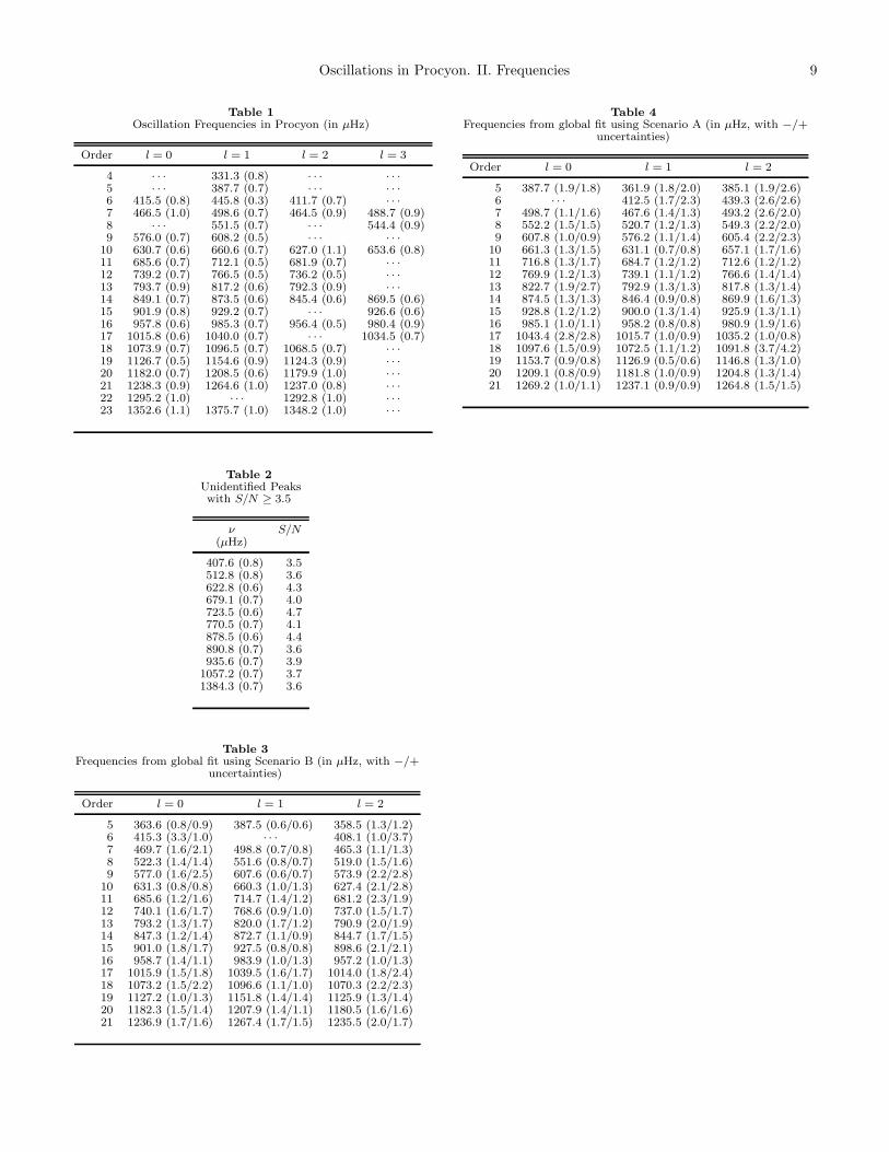
rect l identifications is somewhat subjective. To guidethis process, we used the ridge centroids shown in Fig-ure 9 as well as the small separations δν02 and δν13 fromthe collapsed power spectrum (see Figures 6 and 10).Each frequency extracted using iterative sine-wave fit-ting that lay close to a ridge was assigned an l value andmultiple peaks from the same mode were averaged. Thefinal mode frequencies are listed in Table 1, while peakswith S/N ≥ 3.5 that we have not identified are listed inTable 2. Figures 13 and 14 show these peaks overlaid onthe sidelobe-optimized power spectrum. Figure 15 showsthe three small separations (equations 2–4) as calculatedfrom the frequencies listed in Table 1. The uncertain-ties in the mode frequencies are shown in parentheses inTable 1. These depend on the S/N ratio of the peak andwere calibrated using simulations (e.g., see Bedding et al.2007).The entries in Table 2 are mostly false peaks due to

noise and to residuals from the iterative sine-wave fit-ting, but may include some genuine modes. To check

35 We could also define a small separation δνodd,even to be theamount by which the centroid of the even ridge is offset rightwardsfrom the midpoint of the adjacent odd ridges. This gives similarresults.

6 Bedding et al.

whether some of them may be daily aliases of each otheror of genuine modes, we calculated the differences of allcombinations of frequencies in Tables 1 and 2. The his-togram of these pairwise differences was flat in the vicin-ity of 11.6µHz and showed no excess, confirming thatdaily aliases do not contribute significantly to the list offrequencies in the tables.We also checked whether the number peaks in Table 2

agrees with expectations. We did this by analysing asimulated time series that matched the observations interms of oscillations properties (frequencies, amplitudesand mode lifetimes), noise level, window function anddistribution of weights. We extracted peaks from thesimulated power spectrum using iterative sine-wave fit-ting, as before, and found the number of “extra” peaks(not coinciding with the oscillation ridges) to be simi-lar to that seen in Figure 12. Finally, we remark thatthe peak at 408µHz is a candidate for a mixed modewith l = 1, given that it lies in the same order as thepreviously identified mixed mode at 446µHz (note thatwe expect one extra l = 1 mode to occur at an avoidedcrossing).The modes listed in Table 1 span 20 radial orders and

more than a factor of 4 in frequency. This range is similarto that obtained from long-term studies of the Sun (e.g.,Broomhall et al. 2009) and is unprecedented in astero-seismology. It was made possible by the unusually broadrange of excited modes in Procyon and the high S/N ofour data. Since the stellar background at low frequenciesin intensity measurements is expected to be much higherthan for velocity measurements, it seems unlikely thateven the best data from the Kepler Mission will returnsuch a wide range of frequencies in a single target.

7. MODE LIFETIMES

As discussed in Section 2, if the time series is suf-ficiently long then damping causes each mode in thepower spectrum to be split into a series of peaks un-der a Lorentzian envelope having FWHM Γ = 1/(πτ),where τ is the mode lifetime. Our observations of Pro-cyon are not long enough to resolve the modes into clearLorentzians, and instead we see each mode as a smallnumber of peaks (sometimes one). Furthermore, the cen-troid of these peaks may be offset from the position of thetrue mode, as illustrated in Figure 1 of Anderson et al.(1990). This last feature allows one to use the scatterof the extracted frequencies about smooth ridges in theechelle diagram, calibrated using simulations, to estimatethe mode lifetime (Kjeldsen et al. 2005; Bedding et al.2007). That method cannot be applied to Procyon be-cause the l = 0 and l = 2 ridges are not well-resolvedand the l = 1 ridge is affected by mixed modes.Rather than looking at frequency shifts, we have es-

timated the mode lifetime from the variations in modeamplitudes (again calibrated using simulations). Thismethod is less precise but has the advantage of being in-dependent of the mode identifications (e.g., Leccia et al.2007; Carrier et al. 2007; Bedding et al. 2007). In Pa-per I we calculated the smoothed amplitude curve forProcyon in ten 2-day segments and used the fluctua-tions about the mean to make a rough estimate of themode lifetime: τ = 1.5+1.9

−0.8 days. We have attemptedto improve on that estimate by considering the ampli-tude fluctuations of individual modes, as has been done

for the Sun (e.g., Toutain & Frohlich 1992; Baudin et al.1996; Chang & Gough 1998), but were not able to pro-duce well-calibrated results for Procyon.Instead, we have measured the “peakiness” of the

power spectrum (see Bedding et al. 2007) by calculatingthe ratio between the square of the mean amplitude ofthe 15 highest peaks in the range 500–1300µHz (foundby iterative sine-wave fitting) and the mean power in thesame frequency range. The value for this ratio from ourobservations of Procyon is 6.9. We made a large numberof simulations (3600) having a range of mode lifetimesand with the observed frequency spectrum, noise level,window function and weights. Comparing the simula-tions with the observations led to a mode lifetime forProcyon of 1.29+0.55

−0.49 days.This agrees with the value found in Paper I but is more

precise, confirming that modes in Procyon are signifi-cantly more short-lived than those of the Sun. As dis-cussed in Section 2, the dominant modes in the Sun havelifetimes of 2–4days (e.g., Chaplin et al. 1997). The ten-dency for hotter stars to have shorter mode lifetimes hasrecently been discussed by Chaplin et al. (2009).

8. FITTING TO THE POWER SPECTRUM

Extracting mode parameters by fitting directly to thepower spectrum is widely used in helioseismology, wherethe time series extends continuously for months or evenyears, and so the individual modes are well-resolved (e.g.,Anderson et al. 1990). Mode fitting has not been ap-plied to ground-based observations of solar-type oscil-lations because these data typically have shorter du-rations and significant gaps. Global fitting has beencarried out on spacecraft data, beginning with the 50-d time series of α Cen A taken with the WIRE space-craft (Fletcher et al. 2006) and the 60-d light curve ofHD49933 from CoRoT (Appourchaux et al. 2008). Ourobservations of Procyon are much shorter than either ofthese cases but, given the quality of the data and thespectral window, we considered it worthwhile to attempta fit.Global fits to the Procyon power spectrum were made

by several of us. Here, we present results from a fit usinga Bayesian approach (e.g., Gregory 2005), which allowedus to include in a straightforward way our prior knowl-edge of the oscillation properties. The parameters to beextracted were the frequencies, heights and linewidths ofthe modes. To obtain the marginal probability distri-butions of these parameters and their associated uncer-tainties, we employed an APT MCMC (Automated Par-allel Tempering Markov Chain Monte Carlo) algorithm.It implements the Metropolis-Hastings sampler by per-forming a random walk in parameter space while drawingsamples from the posterior distribution (Gregory 2005).Further details of our implementation of the algorithmwill be given elsewhere (T.L. Campante et al., in prep.).The details of the fitting are as follows:

• The fitting was performed over 17 orders (5–21)using the sidelobe-optimized power spectrum. Ineach order we fitted modes with l = 0, 1, and2, with each individual profile being describedby a symmetric Lorentzian with FWHM Γ andheight H . The mode frequencies were constrainedto lie close to the ridges and to have only small

Oscillations in Procyon. II. Frequencies 7

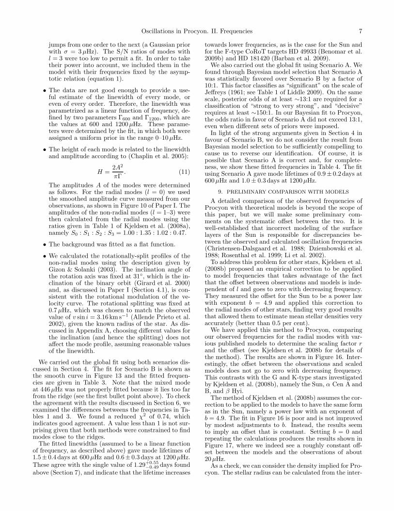
jumps from one order to the next (a Gaussian priorwith σ = 3µHz). The S/N ratios of modes withl = 3 were too low to permit a fit. In order to taketheir power into account, we included them in themodel with their frequencies fixed by the asymp-totic relation (equation 1).

• The data are not good enough to provide a use-ful estimate of the linewidth of every mode, oreven of every order. Therefore, the linewidth wasparametrized as a linear function of frequency, de-fined by two parameters Γ600 and Γ1200, which arethe values at 600 and 1200µHz. These parame-ters were determined by the fit, in which both wereassigned a uniform prior in the range 0–10µHz.

• The height of each mode is related to the linewidthand amplitude according to (Chaplin et al. 2005):

H =2A2

πΓ. (11)

The amplitudes A of the modes were determinedas follows. For the radial modes (l = 0) we usedthe smoothed amplitude curve measured from ourobservations, as shown in Figure 10 of Paper I. Theamplitudes of the non-radial modes (l = 1–3) werethen calculated from the radial modes using theratios given in Table 1 of Kjeldsen et al. (2008a),namely S0 : S1 : S2 : S3 = 1.00 : 1.35 : 1.02 : 0.47.

• The background was fitted as a flat function.

• We calculated the rotationally-split profiles of thenon-radial modes using the description given byGizon & Solanki (2003). The inclination angle ofthe rotation axis was fixed at 31◦, which is the in-clination of the binary orbit (Girard et al. 2000)and, as discussed in Paper I (Section 4.1), is con-sistent with the rotational modulation of the ve-locity curve. The rotational splitting was fixed at0.7µHz, which was chosen to match the observedvalue of v sin i = 3.16km s−1 (Allende Prieto et al.2002), given the known radius of the star. As dis-cussed in Appendix A, choosing different values forthe inclination (and hence the splitting) does notaffect the mode profile, assuming reasonable valuesof the linewidth.

We carried out the global fit using both scenarios dis-cussed in Section 4. The fit for Scenario B is shown asthe smooth curve in Figure 13 and the fitted frequen-cies are given in Table 3. Note that the mixed modeat 446µHz was not properly fitted because it lies too farfrom the ridge (see the first bullet point above). To checkthe agreement with the results discussed in Section 6, weexamined the differences betweens the frequencies in Ta-bles 1 and 3. We found a reduced χ2 of 0.74, whichindicates good agreement. A value less than 1 is not sur-prising given that both methods were constrained to findmodes close to the ridges.The fitted linewidths (assumed to be a linear function

of frequency, as described above) gave mode lifetimes of1.5± 0.4 days at 600µHz and 0.6± 0.3 days at 1200µHz.These agree with the single value of 1.29+0.55

−0.49 days foundabove (Section 7), and indicate that the lifetime increases

towards lower frequencies, as is the case for the Sun andfor the F-type CoRoT targets HD 49933 (Benomar et al.2009b) and HD 181420 (Barban et al. 2009).We also carried out the global fit using Scenario A. We

found through Bayesian model selection that Scenario Awas statistically favored over Scenario B by a factor of10:1. This factor classifies as “significant” on the scale ofJeffreys (1961; see Table 1 of Liddle 2009). On the samescale, posterior odds of at least ∼13:1 are required for aclassification of “strong to very strong”, and “decisive”requires at least ∼150:1. In our Bayesian fit to Procyon,the odds ratio in favor of Scenario A did not exceed 13:1,even when different sets of priors were imposed.In light of the strong arguments given in Section 4 in

favour of Scenario B, we do not consider the result fromBayesian model selection to be sufficiently compelling tocause us to reverse our identification. Of course, it ispossible that Scenario A is correct and, for complete-ness, we show these fitted frequencies in Table 4. The fitusing Scenario A gave mode lifetimes of 0.9± 0.2days at600µHz and 1.0± 0.3 days at 1200µHz.

9. PRELIMINARY COMPARISON WITH MODELS

A detailed comparison of the observed frequencies ofProcyon with theoretical models is beyond the scope ofthis paper, but we will make some preliminary com-ments on the systematic offset between the two. It iswell-established that incorrect modeling of the surfacelayers of the Sun is responsible for discrepancies be-tween the observed and calculated oscillation frequencies(Christensen-Dalsgaard et al. 1988; Dziembowski et al.1988; Rosenthal et al. 1999; Li et al. 2002).To address this problem for other stars, Kjeldsen et al.

(2008b) proposed an empirical correction to be appliedto model frequencies that takes advantage of the factthat the offset between observations and models is inde-pendent of l and goes to zero with decreasing frequency.They measured the offset for the Sun to be a power lawwith exponent b = 4.9 and applied this correction tothe radial modes of other stars, finding very good resultsthat allowed them to estimate mean stellar densities veryaccurately (better than 0.5 per cent).We have applied this method to Procyon, comparing

our observed frequencies for the radial modes with var-ious published models to determine the scaling factor rand the offset (see Kjeldsen et al. 2008b for details ofthe method). The results are shown in Figure 16. Inter-estingly, the offset between the observations and scaledmodels does not go to zero with decreasing frequency.This contrasts with the G and K-type stars investigatedby Kjeldsen et al. (2008b), namely the Sun, α Cen A andB, and β Hyi.The method of Kjeldsen et al. (2008b) assumes the cor-

rection to be applied to the models to have the same formas in the Sun, namely a power law with an exponent ofb = 4.9. The fit in Figure 16 is poor and is not improvedby modest adjustments to b. Instead, the results seemto imply an offset that is constant. Setting b = 0 andrepeating the calculations produces the results shown inFigure 17, where we indeed see a roughly constant off-set between the models and the observations of about20µHz.As a check, we can consider the density implied for Pro-

cyon. The stellar radius can be calculated from the inter-

8 Bedding et al.

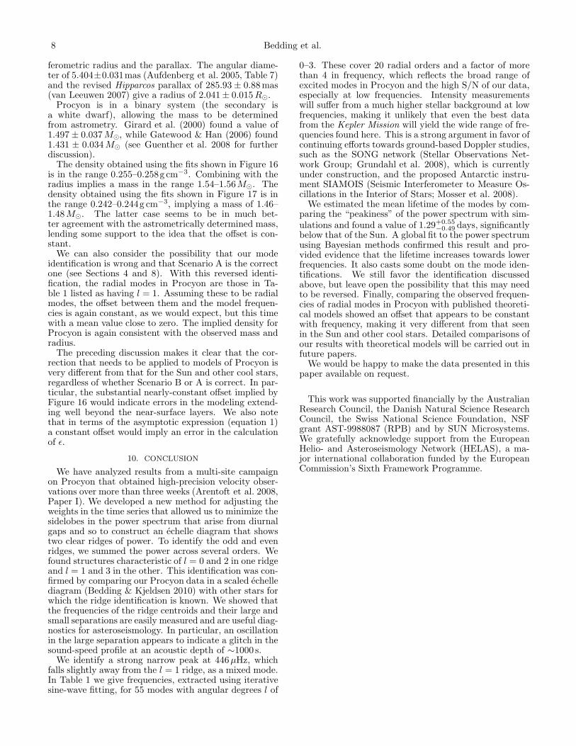
ferometric radius and the parallax. The angular diame-ter of 5.404±0.031mas (Aufdenberg et al. 2005, Table 7)and the revised Hipparcos parallax of 285.93± 0.88mas(van Leeuwen 2007) give a radius of 2.041± 0.015R⊙.Procyon is in a binary system (the secondary is

a white dwarf), allowing the mass to be determinedfrom astrometry. Girard et al. (2000) found a value of1.497± 0.037M⊙, while Gatewood & Han (2006) found1.431 ± 0.034M⊙ (see Guenther et al. 2008 for furtherdiscussion).The density obtained using the fits shown in Figure 16

is in the range 0.255–0.258g cm−3. Combining with theradius implies a mass in the range 1.54–1.56M⊙. Thedensity obtained using the fits shown in Figure 17 is inthe range 0.242–0.244g cm−3, implying a mass of 1.46–1.48M⊙. The latter case seems to be in much bet-ter agreement with the astrometrically determined mass,lending some support to the idea that the offset is con-stant.We can also consider the possibility that our mode

identification is wrong and that Scenario A is the correctone (see Sections 4 and 8). With this reversed identi-fication, the radial modes in Procyon are those in Ta-ble 1 listed as having l = 1. Assuming these to be radialmodes, the offset between them and the model frequen-cies is again constant, as we would expect, but this timewith a mean value close to zero. The implied density forProcyon is again consistent with the observed mass andradius.The preceding discussion makes it clear that the cor-

rection that needs to be applied to models of Procyon isvery different from that for the Sun and other cool stars,regardless of whether Scenario B or A is correct. In par-ticular, the substantial nearly-constant offset implied byFigure 16 would indicate errors in the modeling extend-ing well beyond the near-surface layers. We also notethat in terms of the asymptotic expression (equation 1)a constant offset would imply an error in the calculationof ǫ.

10. CONCLUSION

We have analyzed results from a multi-site campaignon Procyon that obtained high-precision velocity obser-vations over more than three weeks (Arentoft et al. 2008,Paper I). We developed a new method for adjusting theweights in the time series that allowed us to minimize thesidelobes in the power spectrum that arise from diurnalgaps and so to construct an echelle diagram that showstwo clear ridges of power. To identify the odd and evenridges, we summed the power across several orders. Wefound structures characteristic of l = 0 and 2 in one ridgeand l = 1 and 3 in the other. This identification was con-firmed by comparing our Procyon data in a scaled echellediagram (Bedding & Kjeldsen 2010) with other stars forwhich the ridge identification is known. We showed thatthe frequencies of the ridge centroids and their large andsmall separations are easily measured and are useful diag-nostics for asteroseismology. In particular, an oscillationin the large separation appears to indicate a glitch in thesound-speed profile at an acoustic depth of ∼1000 s.We identify a strong narrow peak at 446µHz, which

falls slightly away from the l = 1 ridge, as a mixed mode.In Table 1 we give frequencies, extracted using iterativesine-wave fitting, for 55 modes with angular degrees l of

0–3. These cover 20 radial orders and a factor of morethan 4 in frequency, which reflects the broad range ofexcited modes in Procyon and the high S/N of our data,especially at low frequencies. Intensity measurementswill suffer from a much higher stellar background at lowfrequencies, making it unlikely that even the best datafrom the Kepler Mission will yield the wide range of fre-quencies found here. This is a strong argument in favor ofcontinuing efforts towards ground-based Doppler studies,such as the SONG network (Stellar Observations Net-work Group; Grundahl et al. 2008), which is currentlyunder construction, and the proposed Antarctic instru-ment SIAMOIS (Seismic Interferometer to Measure Os-cillations in the Interior of Stars; Mosser et al. 2008).We estimated the mean lifetime of the modes by com-

paring the “peakiness” of the power spectrum with sim-ulations and found a value of 1.29+0.55

−0.49 days, significantlybelow that of the Sun. A global fit to the power spectrumusing Bayesian methods confirmed this result and pro-vided evidence that the lifetime increases towards lowerfrequencies. It also casts some doubt on the mode iden-tifications. We still favor the identification discussedabove, but leave open the possibility that this may needto be reversed. Finally, comparing the observed frequen-cies of radial modes in Procyon with published theoreti-cal models showed an offset that appears to be constantwith frequency, making it very different from that seenin the Sun and other cool stars. Detailed comparisons ofour results with theoretical models will be carried out infuture papers.We would be happy to make the data presented in this

paper available on request.

This work was supported financially by the AustralianResearch Council, the Danish Natural Science ResearchCouncil, the Swiss National Science Foundation, NSFgrant AST-9988087 (RPB) and by SUN Microsystems.We gratefully acknowledge support from the EuropeanHelio- and Asteroseismology Network (HELAS), a ma-jor international collaboration funded by the EuropeanCommission’s Sixth Framework Programme.

Oscillations in Procyon. II. Frequencies 9

Table 1Oscillation Frequencies in Procyon (in µHz)

Order l = 0 l = 1 l = 2 l = 3

4 · · · 331.3 (0.8) · · · · · ·5 · · · 387.7 (0.7) · · · · · ·6 415.5 (0.8) 445.8 (0.3) 411.7 (0.7) · · ·7 466.5 (1.0) 498.6 (0.7) 464.5 (0.9) 488.7 (0.9)8 · · · 551.5 (0.7) · · · 544.4 (0.9)9 576.0 (0.7) 608.2 (0.5) · · · · · ·

10 630.7 (0.6) 660.6 (0.7) 627.0 (1.1) 653.6 (0.8)11 685.6 (0.7) 712.1 (0.5) 681.9 (0.7) · · ·12 739.2 (0.7) 766.5 (0.5) 736.2 (0.5) · · ·13 793.7 (0.9) 817.2 (0.6) 792.3 (0.9) · · ·14 849.1 (0.7) 873.5 (0.6) 845.4 (0.6) 869.5 (0.6)15 901.9 (0.8) 929.2 (0.7) · · · 926.6 (0.6)16 957.8 (0.6) 985.3 (0.7) 956.4 (0.5) 980.4 (0.9)17 1015.8 (0.6) 1040.0 (0.7) · · · 1034.5 (0.7)18 1073.9 (0.7) 1096.5 (0.7) 1068.5 (0.7) · · ·19 1126.7 (0.5) 1154.6 (0.9) 1124.3 (0.9) · · ·20 1182.0 (0.7) 1208.5 (0.6) 1179.9 (1.0) · · ·21 1238.3 (0.9) 1264.6 (1.0) 1237.0 (0.8) · · ·22 1295.2 (1.0) · · · 1292.8 (1.0) · · ·23 1352.6 (1.1) 1375.7 (1.0) 1348.2 (1.0) · · ·

Table 2Unidentified Peakswith S/N ≥ 3.5

ν S/N(µHz)

407.6 (0.8) 3.5512.8 (0.8) 3.6622.8 (0.6) 4.3679.1 (0.7) 4.0723.5 (0.6) 4.7770.5 (0.7) 4.1878.5 (0.6) 4.4890.8 (0.7) 3.6935.6 (0.7) 3.9

1057.2 (0.7) 3.71384.3 (0.7) 3.6

Table 3Frequencies from global fit using Scenario B (in µHz, with −/+

uncertainties)

Order l = 0 l = 1 l = 2

5 363.6 (0.8/0.9) 387.5 (0.6/0.6) 358.5 (1.3/1.2)6 415.3 (3.3/1.0) · · · 408.1 (1.0/3.7)7 469.7 (1.6/2.1) 498.8 (0.7/0.8) 465.3 (1.1/1.3)8 522.3 (1.4/1.4) 551.6 (0.8/0.7) 519.0 (1.5/1.6)9 577.0 (1.6/2.5) 607.6 (0.6/0.7) 573.9 (2.2/2.8)

10 631.3 (0.8/0.8) 660.3 (1.0/1.3) 627.4 (2.1/2.8)11 685.6 (1.2/1.6) 714.7 (1.4/1.2) 681.2 (2.3/1.9)12 740.1 (1.6/1.7) 768.6 (0.9/1.0) 737.0 (1.5/1.7)13 793.2 (1.3/1.7) 820.0 (1.7/1.2) 790.9 (2.0/1.9)14 847.3 (1.2/1.4) 872.7 (1.1/0.9) 844.7 (1.7/1.5)15 901.0 (1.8/1.7) 927.5 (0.8/0.8) 898.6 (2.1/2.1)16 958.7 (1.4/1.1) 983.9 (1.0/1.3) 957.2 (1.0/1.3)17 1015.9 (1.5/1.8) 1039.5 (1.6/1.7) 1014.0 (1.8/2.4)18 1073.2 (1.5/2.2) 1096.6 (1.1/1.0) 1070.3 (2.2/2.3)19 1127.2 (1.0/1.3) 1151.8 (1.4/1.4) 1125.9 (1.3/1.4)20 1182.3 (1.5/1.4) 1207.9 (1.4/1.1) 1180.5 (1.6/1.6)21 1236.9 (1.7/1.6) 1267.4 (1.7/1.5) 1235.5 (2.0/1.7)

Table 4Frequencies from global fit using Scenario A (in µHz, with −/+

uncertainties)

Order l = 0 l = 1 l = 2

5 387.7 (1.9/1.8) 361.9 (1.8/2.0) 385.1 (1.9/2.6)6 · · · 412.5 (1.7/2.3) 439.3 (2.6/2.6)7 498.7 (1.1/1.6) 467.6 (1.4/1.3) 493.2 (2.6/2.0)8 552.2 (1.5/1.5) 520.7 (1.2/1.3) 549.3 (2.2/2.0)9 607.8 (1.0/0.9) 576.2 (1.1/1.4) 605.4 (2.2/2.3)

10 661.3 (1.3/1.5) 631.1 (0.7/0.8) 657.1 (1.7/1.6)11 716.8 (1.3/1.7) 684.7 (1.2/1.2) 712.6 (1.2/1.2)12 769.9 (1.2/1.3) 739.1 (1.1/1.2) 766.6 (1.4/1.4)13 822.7 (1.9/2.7) 792.9 (1.3/1.3) 817.8 (1.3/1.4)14 874.5 (1.3/1.3) 846.4 (0.9/0.8) 869.9 (1.6/1.3)15 928.8 (1.2/1.2) 900.0 (1.3/1.4) 925.9 (1.3/1.1)16 985.1 (1.0/1.1) 958.2 (0.8/0.8) 980.9 (1.9/1.6)17 1043.4 (2.8/2.8) 1015.7 (1.0/0.9) 1035.2 (1.0/0.8)18 1097.6 (1.5/0.9) 1072.5 (1.1/1.2) 1091.8 (3.7/4.2)19 1153.7 (0.9/0.8) 1126.9 (0.5/0.6) 1146.8 (1.3/1.0)20 1209.1 (0.8/0.9) 1181.8 (1.0/0.9) 1204.8 (1.3/1.4)21 1269.2 (1.0/1.1) 1237.1 (0.9/0.9) 1264.8 (1.5/1.5)

10 Bedding et al.

Figure 1. Weights for time series of velocity observations of Procyon, optimized to minimize: (a) the noise level and (b) the height of thesidelobes.

Figure 2. Power spectrum of oscillations in Procyon: (a) using the noise-optimized weights; (b) using the sidelobe-optimized weights;(c) using the sidelobe-optimized weights and smoothing by convolution with a Gaussian with FWHM 2µHz.

Oscillations in Procyon. II. Frequencies 11

Figure 3. Spectral window for the Procyon observations using(a) noise-optimized weights and (b) sidelobe-optimized weights.

Figure 4. Power spectrum of Procyon in echelle format usinga large separation of 56µHz, based on the sidelobe-optimizedweights. Two ridges are clearly visible. The upper parts are verti-cal but the lower parts are tilted, indicating a change in the largeseparation as a function of frequency. The orders are numberedsequentially on the right-hand side.

Figure 5. Same as Fig. 4, but for the noise-optimized weights.The sidelobes from daily aliasing mean that the ridges can no longerbe clearly distinguished.

Figure 6. The power spectrum of Procyon collapsed along severalorders. Note that the power spectrum was first smoothed slightlyby convolving with a Gaussian with FWHM 0.5µHz. The dottedlines are separated by exactly ∆ν/2, to guide the eye in assessingthe 0–1 small separation

12 Bedding et al.

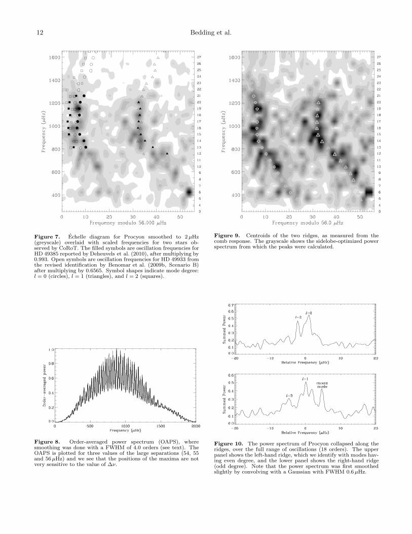
Figure 7. Echelle diagram for Procyon smoothed to 2µHz(greyscale) overlaid with scaled frequencies for two stars ob-served by CoRoT. The filled symbols are oscillation frequencies forHD 49385 reported by Deheuvels et al. (2010), after multiplying by0.993. Open symbols are oscillation frequencies for HD 49933 fromthe revised identification by Benomar et al. (2009b, Scenario B)after multiplying by 0.6565. Symbol shapes indicate mode degree:l = 0 (circles), l = 1 (triangles), and l = 2 (squares).

Figure 8. Order-averaged power spectrum (OAPS), wheresmoothing was done with a FWHM of 4.0 orders (see text). TheOAPS is plotted for three values of the large separations (54, 55and 56µHz) and we see that the positions of the maxima are notvery sensitive to the value of ∆ν.

Figure 9. Centroids of the two ridges, as measured from thecomb response. The grayscale shows the sidelobe-optimized powerspectrum from which the peaks were calculated.

Figure 10. The power spectrum of Procyon collapsed along theridges, over the full range of oscillations (18 orders). The upperpanel shows the left-hand ridge, which we identify with modes hav-ing even degree, and the lower panel shows the right-hand ridge(odd degree). Note that the power spectrum was first smoothedslightly by convolving with a Gaussian with FWHM 0.6µHz.

Oscillations in Procyon. II. Frequencies 13

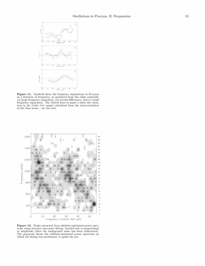
Figure 11. Symbols show the frequency separations in Procyonas a function of frequency, as measured from the ridge centroids:(a) large frequency separation, (b) second differences, and (c) smallfrequency separation. The dotted lines in panel a show the varia-tion in ∆ν (with ±1σ range) calculated from the autocorrelationof the time series – see the text.

Figure 12. Peaks extracted from sidelobe-optimized power spec-trum using iterative sine-wave fitting. Symbol size is proportionalto amplitude (after the background noise has been subtracted).The grayscale shows the sidelobe-optimized power spectrum onwhich the fitting was performed, to guide the eye.

14 Bedding et al.

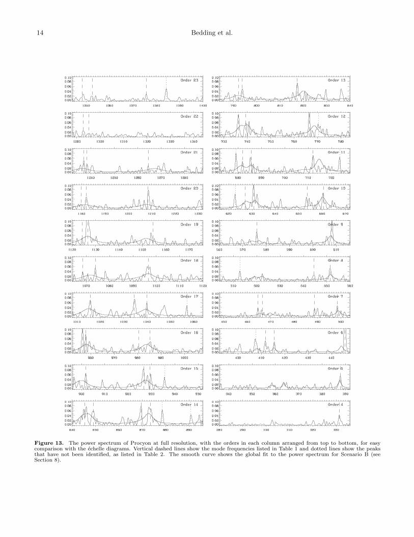
Figure 13. The power spectrum of Procyon at full resolution, with the orders in each column arranged from top to bottom, for easycomparison with the echelle diagrams. Vertical dashed lines show the mode frequencies listed in Table 1 and dotted lines show the peaksthat have not been identified, as listed in Table 2. The smooth curve shows the global fit to the power spectrum for Scenario B (seeSection 8).

Oscillations in Procyon. II. Frequencies 15

Figure 14. The power spectrum of Procyon overlaid with modefrequencies listed in Table 1. Symbols indicate angular degree(squares: l = 0; diamonds: l = 1; crosses: l = 2; pluses: l = 3).Asterisks show the peaks that have not been identified, as listed inTable 2.

Figure 15. Small frequency separations in Procyon, as measuredfrom the mode frequencies listed in Table 1.

Figure 16. The difference between observed frequencies of radialmodes in Procyon and those of scaled models. The symbols in-dicate different models, as follows: squares from Chaboyer et al.(1999, Table 2), crosses from Di Mauro & Christensen-Dalsgaard(2001), asterisks from Kervella et al. (2004, Table 4), and trian-gles from Eggenberger et al. (2005, model M1a). In each case, thedotted curve shows the correction calculated using equation (4) ofKjeldsen et al. (2008b).

Figure 17. Same as Figure 16, but with a constant near-surfacecorrection (b = 0).

16 Bedding et al.

REFERENCES

Aerts, C., Christensen-Dalsgaard, J., Cunha, M., & Kurtz, D. W.2008, Sol. Phys., 251, 3

Aizenman, M., Smeyers, P., & Weigert, A. 1977, A&A, 58, 41Allende Prieto, C., Asplund, M., Lopez, R. J. G., & Lambert,

D. L. 2002, ApJ, 567, 544Anderson, E. R., Duvall, T. L., & Jefferies, S. M. 1990, ApJ, 364,

699Appourchaux, T., et al. 2008, A&A, 488, 705Arentoft, T., Kjeldsen, H., & Bedding, T. R. 2010, in GONG

2008/SOHO XXI Meeting on Solar-Stellar Dynamos asaRevealed by Helio- and Asterseismology, ed. M. Dikpati,I. Gonzalez-Hernandez, T. Arentoft, & F. Hill (ASP Conf.Ser.), in press (arXiv:0901.3632)

Arentoft, T., Kjeldsen, H., Bedding, T. R., et al. 2008, ApJ, 687,1180, (Paper I)

Aufdenberg, J. P., Ludwig, H.-G., & Kervella, P. 2005, ApJ, 633,424

Ballot, J., Garcıa, R. A., & Lambert, P. 2006, MNRAS, 369, 1281Ballot, J., Turck-Chieze, S., & Garcıa, R. A. 2004, A&A, 423,

1051Barban, C., Michel, E., Martic, M., Schmitt, J., Lebrun, J. C.,

Baglin, A., & Bertaux, J. L. 1999, A&A, 350, 617Barban, C., et al. 2009, A&A, 506, 51Baudin, F., Gabriel, A., Gibert, D., Palle, P. L., & Regulo, C.

1996, A&A, 311, 1024Bedding, T. R., & Kjeldsen, H. 2003, PASA, 20, 203Bedding, T. R., & Kjeldsen, H. 2007, in Unsolved Problems in

Stellar Physics: A Conference in Honour of Douglas Gough,AIP Conf. Proc., vol. 948, ed. R. J. Stancliffe, G. Houdek,R. G. Martin, & C. A. Tout, 117

—. 2010, Commun. Asteroseismology, 161, 3Bedding, T. R., Kjeldsen, H., Arentoft, T., et al. 2007, ApJ, 663,

1315Bedding, T. R., Kjeldsen, H., Butler, R. P., McCarthy, C., Marcy,

G. W., O’Toole, S. J., Tinney, C. G., & Wright, J. T. 2004,ApJ, 614, 380

Bedding, T. R., et al. 2010, ApJ Lett., in press (arXiv:1001.0229)Benomar, O., Appourchaux, T., & Baudin, F. 2009a, A&A, 506,

15Benomar, O., et al. 2009b, A&A, 507, L13Bonanno, A., Kuker, M., & Paterno, L. 2007, A&A, 462, 1031Broomhall, A.-M., Chaplin, W. J., Davies, G. R., Elsworth, Y.,

Fletcher, S. T., Hale, S. J., Miller, B., & New, R. 2009,MNRAS, 396, L100

Brown, T. M., & Gilliland, R. L. 1994, ARA&A, 32, 37Carrier, F., et al. 2007, A&A, 470, 1059—. 2010, A&A, 55, A73Chaboyer, B., Demarque, P., & Guenther, D. B. 1999, ApJ, 525,

L41Chang, H.-Y., & Gough, D. O. 1998, Sol. Phys., 181, 251Chaplin, W. J., Elsworth, Y., Isaak, G. R., McLeod, C. P., Miller,

B. A., & New, R. 1997, MNRAS, 288, 623Chaplin, W. J., Houdek, G., Elsworth, Y., Gough, D. O., Isaak,

G. R., & New, R. 2005, MNRAS, 360, 859Chaplin, W. J., Houdek, G., Karoff, C., Elsworth, Y., & New, R.

2009, A&A, 500, L21Christensen-Dalsgaard, J. 2004, Sol. Phys., 220, 137Christensen-Dalsgaard, J., Dappen, W., & Lebreton, Y. 1988,

Nat, 336, 634Christensen-Dalsgaard, J., & Houdek, G. 2009, Ap&SS, in press

(arXiv:0911.4629)Deheuvels, S., et al. 2010, A&A, submittedDi Mauro, M. P., & Christensen-Dalsgaard, J. 2001, in IAU

Symposium 203: Recent Insights into the Physics of the Sunand Heliosphere: Highlights from SOHO and Other SpaceMissions, ed. P. Brekke, B. Fleck, & J. B. Gurman (ASP Conf.Ser.), 94

Dziembowski, W. A., Paterno, L., & Ventura, R. 1988, A&A, 200,213

Eggenberger, P., Carrier, F., & Bouchy, F. 2005, NewA, 10, 195Eggenberger, P., Carrier, F., Bouchy, F., & Blecha, A. 2004,

A&A, 422, 247

Fletcher, S. T., Chaplin, W. J., Elsworth, Y., Schou, J., & Buzasi,D. 2006, MNRAS, 371, 935

Frandsen, S., Jones, A., Kjeldsen, H., Viskum, M., Hjorth, J.,Andersen, N. H., & Thomsen, B. 1995, A&A, 301, 123

Garcıa, R. A., et al. 2009, A&A, 506, 41Gatewood, G., & Han, I. 2006, AJ, 131, 1015Gilliland, R. L., et al. 1993, AJ, 106, 2441Gilliland, R. L., et al. 2010, PASP, 122, 131Girard, T. M., Wu, H., Lee, J. T., Dyson, S. E., van Altena,

W. F., et al. 2000, AJ, 119, 2428Gizon, L., & Solanki, S. K. 2003, ApJ, 589, 1009Gough, D. O. 1986, in Hydrodynamic and Magnetodynamic

Problems in the Sun and Stars, ed. Y. Osaki (Tokyo: Uni. ofTokyo Press), 117

Gough, D. O. 1990, in Lecture Notes in Physics, Vol. 367,Progress of Seismology of the Sun and Stars, ed. Y. Osaki &H. Shibahashi (Berlin: Springer), 283

Grec, G., Fossat, E., & Pomerantz, M. A. 1983, Sol. Phys., 82, 55Gregory, P. C. 2005, Bayesian Logical Data Analysis for the

Physical Sciences (Cambridge University Press)Gruberbauer, M., Kallinger, T., Weiss, W. W., & Guenther, D. B.

2009, A&A, 506, 1043Grundahl, F., Christensen-Dalsgaard, J., Arentoft, T., Frandsen,

S., Kjeldsen, H., Jørgensen, U. G., & Kjaergaard, P. 2008,Commun. Asteroseismology, 157, 273

Guenther, D. B., & Demarque, P. 1993, ApJ, 405, 298Guenther, D. B., et al. 2008, ApJ, 687, 1448Hogbom, J. A., & Brouw, W. N. 1974, A&A, 33, 289Houdek, G., & Gough, D. O. 2007, MNRAS, 375, 861Jeffreys, H. 1961, Theory of Probability, 3rd edn. (New York:

Oxford University Press)Kallinger, T., Gruberbauer, M., Guenther, D. B., Fossati, L., &

Weiss, W. W. 2010, A&A, 510, A106Karoff, C. 2007, MNRAS, 381, 1001Kervella, P., Thevenin, F., Morel, P., Berthomieu, G., Borde, P.,

& Provost, J. 2004, A&A, 413, 251Kjeldsen, H., Bedding, T. R., Arentoft, T., et al. 2008a, ApJ, 682,

1370Kjeldsen, H., Bedding, T. R., & Christensen-Dalsgaard, J. 2008b,

ApJ, 683, L175Kjeldsen, H., Bedding, T. R., Viskum, M., & Frandsen, S. 1995,

AJ, 109, 1313Kjeldsen, H., et al. 2005, ApJ, 635, 1281Leccia, S., Kjeldsen, H., Bonanno, A., Claudi, R. U., Ventura, R.,

& Paterno, L. 2007, A&A, 464, 1059Li, L. H., Robinson, F. J., Demarque, P., Sofia, S., & Guenther,

D. B. 2002, ApJ, 567, 1192Liddle, A. R. 2009, Annual Review of Nuclear and Particle

Science, 59, 95Martic, M., Lebrun, J.-C., Appourchaux, T., & Korzennik, S. G.

2004, A&A, 418, 295Martic, M., et al. 1999, A&A, 351, 993Mathur, S., et al. 2010, A&A, submittedMichel, E., et al. 2008, Science, 322, 558Mosser, B., & Appourchaux, T. 2009, A&A, 508, 877Mosser, B., Appourchaux, T., Catala, C., Buey, J., & SIAMOIS

team. 2008, Journal of Physics Conference Series, 118, 012042Mosser, B., Maillard, J. P., Mekarnia, D., & Gay, J. 1998, A&A,

340, 457Osaki, J. 1975, PASJ, 27, 237Provost, J., Berthomieu, G., Martic, M., & Morel, P. 2006, A&A,

460, 759Regulo, C., & Roca Cortes, T. 2005, A&A, 444, L5Rosenthal, C. S., Christensen-Dalsgaard, J., Nordlund, A., Stein,

R. F., & Trampedach, R. 1999, A&A, 351, 689Roxburgh, I. W. 2009, A&A, 506, 435Roxburgh, I. W., & Vorontsov, S. V. 2006, MNRAS, 369, 1491Tassoul, M. 1980, ApJS, 43, 469Toutain, T., & Frohlich, C. 1992, A&A, 257, 287van Leeuwen, F. 2007, Hipparcos, the New Reduction of the Raw

Data (Springer: Dordrecht)

Oscillations in Procyon. II. Frequencies 17

APPENDIX

A. ROTATIONAL SPLITTING

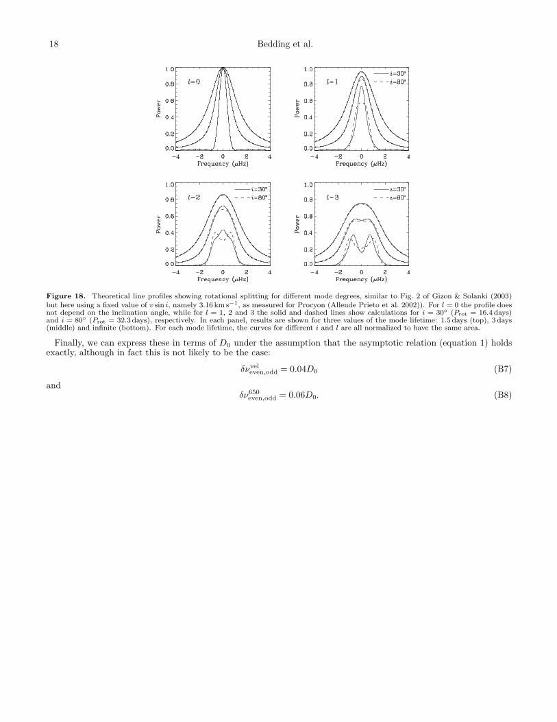
We expect non-radial modes to be split due to the rotation of the star. The rotation period of Procyon is not known,although slow variations in our velocity observations (Paper I) indicated a value of either 10.3 days or twice that value.The projected rotational velocity has been measured spectroscopically. Allende Prieto et al. (2002) determined a valueof v sin i = 3.16± 0.50km s−1, although they note that the actual value may be lower by about 0.5 km s−1.Gizon & Solanki (2003) have studied the effect of rotation on the profiles of solar-like oscillations as a function of

inclination and mode lifetime (see also Ballot et al. 2006). We have repeated their calculations for our observations ofProcyon (with sidelobe-optimized weights). The results are shown in Figure 18, which shows the effects of rotationalsplitting, inclination angle and mode lifetime on the theoretical profile of the modes.36 Note that the calculations do notinclude the stochastic nature of the excitation and so the function shown here should properly be called the expectationvalue of the power spectrum, also known as the limit spectrum. Figure 18 is similar to Figure 2 of Gizon & Solanki(2003) except that instead of fixing the rotation period, we have fixed v sin i to be the measured value. For l = 0 theprofile does not depend on the inclination angle, while for l = 1, 2 and 3 the solid and dashed lines show calculationsfor i = 30◦ (Prot = 16.4days) and i = 80◦ (Prot = 32.3days), respectively. In each panel, results are shown for threevalues of the mode lifetime: 1.5 days (top), 3 days (middle) and infinite (bottom). For each mode lifetime, the curvesfor different i and l are all normalized to have the same area.We see from Figure 18 that for a fixed v sin i, the width of the profile stays roughly constant as a function of

inclination. If the rotation axis of the star happens to be in the plane of the sky (i = 90◦) then the rotation periodis too low to produce a measurable splitting. At the other extreme, if the inclination is small (so that the rotation isclose to pole-on), then the rotational splitting will be large but most of the power will be in the central peak (m = 0).Either way, once the profile has been broadened by the mode lifetime, the splitting will be unobservable.We conclude that for realistic values of the mode lifetime, our observations are not long enough to detect rotational

splitting in Procyon. The line profiles are broadened by rotation, but it is not possible to disentangle the rotation ratefrom the inclination angle. Rotational splitting is not measurable in Procyon, except perhaps with an extremely longdata set. The detection of rotational splitting requires choosing a star with a larger v sin i or a longer mode lifetime,or both.

B. RELATING RIDGE CENTROIDS TO MODE FREQUENCIES

As discussed in Section 5, the frequencies of the ridge centroids are useful for asteroseismology in cases where it isdifficult to resolve the ridges into their component modes. In this appendix, we relate the frequencies of the ridgecentroids to those of the underlying modes, which allows us to express the small separation of the ridges (equation 10)in terms of the conventional small separations (δν01, δν02, and δν13). These relationships will allow the observationsto be compared with theoretical models.The ridge centroids depend on the relative contributions of modes with l = 0, 1, 2, and 3. The power in the even

ridge is approximately equally divided between l = 0 and l = 2, while the odd ridge is dominated by l = 1 but withsome contribution from l = 3. The exact ratios depend on the observing method, as discussed by Kjeldsen et al.(2008a). For velocity measurements, such as those presented in this paper for Procyon, the amplitude ratios given byKjeldsen et al. (2008a, their Table 1) yield the following expressions for the centroids in power:

νveln,even=0.49νn,0 + 0.51νn−1,2 (B1)

νveln,odd=0.89νn,1 + 0.11νn−1,3, (B2)

where the superscript indicates these apply to velocity measurements.For photometric measurements, such as those currently being obtained with the CoRoT and Kepler Missions, the

relative contributions from the various l values are different. Table 1 of Kjeldsen et al. (2008a) gives response factorsfor intensity measurements in the three VIRGO passbands, namely 402, 500 and 862nm. For CoRoT and Kepler, itis appropriate to use a central wavelength of 650nm. Using the same method as Kjeldsen et al. (2008a), we find theratios (in amplitude) for this case to be S0 : S1 : S2 : S3 = 1.00 : 1.23 : 0.71 : 0.14. The ridge centroids measured fromsuch data would then be

ν650n,even=0.66νn,0 + 0.34νn−1,2 (B3)

ν650n,odd=0.99νn,1 + 0.01νn−1,3, (B4)

We can express the new small separation of the ridge centroids (equation 10) in terms of the conventional ones. Forvelocity we have

δνveleven,odd = δν01 − 0.51δν02 + 0.11δν13. (B5)

and for photometry we have

δν650even,odd = δν01 − 0.34δν02 + 0.01δν13. (B6)

36 Note that we have made the quite reasonable assumption that the internal rotation has a similar period to the surface rotation.

18 Bedding et al.

Figure 18. Theoretical line profiles showing rotational splitting for different mode degrees, similar to Fig. 2 of Gizon & Solanki (2003)but here using a fixed value of v sin i, namely 3.16 km s−1, as measured for Procyon (Allende Prieto et al. 2002)). For l = 0 the profile doesnot depend on the inclination angle, while for l = 1, 2 and 3 the solid and dashed lines show calculations for i = 30◦ (Prot = 16.4 days)and i = 80◦ (Prot = 32.3 days), respectively. In each panel, results are shown for three values of the mode lifetime: 1.5 days (top), 3 days(middle) and infinite (bottom). For each mode lifetime, the curves for different i and l are all normalized to have the same area.

Finally, we can express these in terms of D0 under the assumption that the asymptotic relation (equation 1) holdsexactly, although in fact this is not likely to be the case:

δνveleven,odd = 0.04D0 (B7)

andδν650even,odd = 0.06D0. (B8)