Med Biol Eng Comput manuscript No.(will be inserted by the editor)

Andreas Kuhn · Thierry Keller · Marc Lawrence ·

Manfred Morari

A model for current regulated transcutaneous electrical

stimulation: Simulations and experiments

Received: / Accepted:

Abstract Complex nerve models have been developed for describing the generation of action potentials in

humans. Such nerve models have primarily been used to model implantable electrical stimulation systems,

where the stimulation electrodes are close to the nerve (near-field). To address if these nerve models can also

be used to model transcutaneous electrical stimulation (TES) (far-field), we have developed a TES model

that comprises a volume conductor and different previously published non-linear nerve models. The volume

conductor models the resistive and capacitive properties of electrodes, electrode-skin interface, skin, fat, mus-

Andreas Kuhn · Thierry Keller · Marc Lawrence · Manfred Morari

Automatic Control Laboratory, ETH Zurich

Physikstrasse 3

CH-8092 Zurich

Tel.: +41 44 632 6571

Fax: +41 44 632 1211

E-mail: kuhnan@control.ee.ethz.ch

Andreas Kuhn · Thierry Keller · Marc Lawrence

Sensory-Motor Systems Laboratory, ETH Zurich

CH-8092 Zurich

Number of words: 4923

Number of words (abstract): 167

2

cle, and bone. The non-linear nerve models were used to conclude from the potential field within the volume

conductor on nerve activation. A comparison of simulated and experimentally measured chronaxie values (a

measure for the excitability of nerves) and muscle twitch forces on human volunteers allowed us to conclude

that some of the published nerve models can be used in TES models. The presented TES model provides a

first step to more extensive model implementations for TES in which e.g., multi-array electrode configurations

can be tested.

Keywords Transcutaneous electrical stimulation · finite element model · active nerve model · capacitive

effects

1 Introduction

Transcutaneous electrical stimulation (TES) can be used to artificially activate nerve and muscle fibers by

applying electrical current pulses between pairs of electrodes placed on the skin surface. The applied current

flows through the skin and underlying tissues (bulk tissues) where a spatiotemporal potential field is generated

depending on the resistivities and permittivities (capacitance) of the various tissues. Axons distributed in nerve

bundles that lie within the bulk tissues experience activation and can generate action potentials (APs) due to

the electrically induced potential field. These APs travel along the axons to the muscle where a contraction

of the muscle is generated. For single stimulation pulses the generated twitch force is increased when the

pulse amplitude or the pulse duration (PD) is increased [2] because additional axons are recruited in the nerve

bundles [45].

Two-step models have been proposed to describe nerve activation in TES [38]. The first step describes

the electrical potential field within the electrodes, the electrode-skin interfaces, and the bulk tissues (volume

conductor). Analytical models [32, 39] finite difference models [34], and finite element (FE) models [35] were

used to calculate the potential field in the volume conductor. The second step describes the complex behavior

of the axons’ transmembrane potential (TP), which depends upon the spatiotemporal potential field along

the axon [37]. Several two step models were proposed to describe TES [43, 51, 27]. However, these models

exclusively employ static models (i.e. neglecting capacitive effects) to describe the volume conductor, and

linear nerve models to describe nerve activation. Up to now non-linear nerve models, which can describe more

facets of nerve activation [45], were mainly used for implantable systems [31, 49, 47], epidural stimulation

3

[18], or motor cortex stimulation [33], where the exciting electrodes are small and close to the nerve (near-

field). To address if these nerve models can also be used to model TES (far-field), we have developed a

TES model that comprises a volume conductor and different non-linear nerve models. Such a model that

describes TES from the applied stimulation current pulse to nerve recruitment is useful for the development

and enhancement of new stimulation technology. For example, the irregular potential fields that are delivered

with multi-channel array electrodes [8, 30] can be described using such models. These irregular potential

fields produced with multi-channel array electrodes can be varied spatially and temporally and require time

varying solutions to describe nerve activation appropriately. In this paper a suitable axon model to be used in

such a TES model is identified and verified with experiments.

A method to experimentally verify electrical stimulation models is to compare simulated strength-duration

curves with experimentally obtained strength-duration data [52]. Strength-duration curves describe the stim-

ulation current amplitude versus the PD for threshold activation. From strength-duration curves rheobase and

chronaxie can be derived [13]. The rheobase is the smallest current amplitude of ’infinite’ duration (practically,

a few hundred milliseconds) that produces an activation. Chronaxie is the PD required for activation with an

amplitude of two times the rheobase. Experimentally obtained chronaxie values using electrodes placed close

to the excited axon (clamp experiments, animal studies and needle electrodes) are between 30 µs and 150 µs

[9, 3, 42]. Published non-linear nerve models were experimentally verified in this range of chronaxie values

[38, 4, 52, 42, 37]. However, chronaxie values that were obtained experimentally using surface electrodes are

longer. In humans the chronaxie values using surface electrodes were found to be between 200 µs and 700 µs

[48, 15, 23]. It is unclear if the short chronaxie values (30 - 150 µs) of such non-linear nerve models that were

designed for implantable systems are increased significantly when used in a TES model to describe chronaxie

values measured with surface electrodes in TES (200 - 700 µs).

Apart from strength-duration curves, which describe only the excitability at motor threshold (thickest

axons activated), measured force or torque versus PD curves were used to describe the excitability of nerves

(where also thinner axons are activated) [45]. Such measurements at higher stimulation intensities provide

additionally an understanding of the nerve recruitment. These curves show either the stimulation amplitude

versus the PD at a fixed force output [54, 6, 22] or the force versus the PD at a fixed amplitude [1, 14]. The

influence of the muscle properties on the measurement can be minimized by measuring twitch forces (single

4

stimulation pulse) instead of tetanic forces [2]. This has the advantage that experimentally measured twitch

forces can be directly compared with nerve recruitment obtained from nerve models [31]. As such, we present

twitch force measurements on human volunteers that are compared with the nerve recruitment from our TES

model. This comparison enabled us to conclude, which nerve models are most suitable to be used in TES

models.

2 Methods

2.1 TES model

The developed TES model comprises an FE model that describes the potential field in the volume conductor

(forearm) and an active (non-linear) nerve model that calculates nerve activation. The following two subsec-

tions introduce the two models and how they are linked together.

Finite element model

The electric scalar potential (VFE) within the arm model (volume conductor) and the electrodes was described

by Equation (1), which can be derived from Amperes’s Law. It takes into account both the resistive (σ) and the

dielectric properties (ε = ε0εr) of the tissues. The electrical potentials were calculated with the finite element

time domain (FETD) solver of the FEM package Ansys (EMAG, Ansys Inc., Canonsburg, PA).

−∇ · ([σ]∇VFE)−∇([ε]∇∂VFE

∂t) = 0 (1)

The two stimulation electrodes were modeled as a good conducting substrate (conductive carbon rubber)

with a 1 mm thick electrode-skin interface layer (hydrogel) with a size of 5 cm by 5 cm and a center to center

spacing of 11 cm. These parameters were chosen as in the experimental setup (section 2.2). The amplitudes

and durations of the current-regulated pulses that were applied to the electrodes could be varied. The bulk

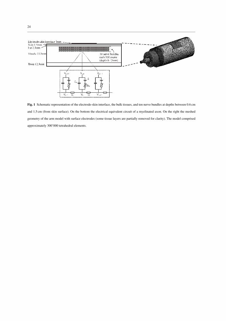
tissues were modeled with a multiple layer cylinder (Fig. 1) representing the forearm. A comparison of a

cylindrical model geometry with a more detailed geometry segmented from MRI scans, revealed that nerve

activation did not change significantly (<5%) using the more detailed geometry [26]. Therefore, a cylindrical

geometry was used comprising skin, fat, muscle and bone layers with the thicknesses of 1.5 mm (skin), 2.5 mm

(fat), 33.5 mm (muscle), 6 mm (cortical bone) and 6.5 mm (bone marrow). The cylinder had a length of 40 cm.

5

The FE model was verified in [24] with experimental measurements where the potential on the skin and the

potential in the muscle were measured and compared.

The electrical properties (resistive and capacitive) that were used for the tissues and electrodes are given

in Table 1. The anisotropy of the muscles’ resistivity and permittivity was considered using a factor of three

between the axial and longitudinal direction [45].

The resulting time dependent potential field of the FE model was interpolated onto lines at different depths,

which represented nerve bundle locations that were parallel to the longitudinal axis of the arm model. The

potential at time t and position n on one nerve line is labelled VFE,n(t).

Nerve models

Four different active axon models (see Table 2) were combined with the FE model. These myelinated axon

models were chosen to cover different axon model structures and a wide range of chronaxie values (near-field)

[55] (published chronaxie values are given in Table 2). Models A and B are based on the Frankenhaeuser-

Huxley membrane [11] that describe sodium, potassium, and leakage membrane currents [38] of the nodes

of Ranvier. Model C is the CRRSS model (CRRSS stands for its authors’ names) that only incorporates

sodium and leakage currents at the nodes of Ranvier. The CRRSS membrane is similar to the Hudgkin-

Huxley membrane [17] but without potassium channels because they were found to be less important in the

excitation process of myelinated mammalian nerves [52]. Model D (MRG model) incorporates a double cable

structure that does not only describe membrane currents at the nodes of Ranvier but also at the paranodal and

internodal sections [37].

The four introduced axon models describe the TP of a single axon with a certain diameter. However,

in humans axons are gathered in nerve bundles consisting of many axons with different diameters. Multiple

nerve bundles innervate muscles and these nerve bundles lie in different depth within the body [50]. Therefore,

the four axon models (Table 2) were joined to multiple nerve bundles that lie in different depths underneath

the stimulating electrode. The nerve bundles had a length of 15 cm and were centered under the cathode

at depths (from skin) between 0.6 cm and 1.5 cm with 0.1 cm spacing (see Fig. 1). Each of the ten nerve

bundles consisted of 100 axons with diameters distributed according to the bimodal distribution in human

nerve bundles with peaks at 6 µm and 13 µm [46, 41]. The minimal axon diameter was 4 µm and the maximal

diameter was 16 µm. Recruitment Rec was defined as the percentage of axons that were activated in all

6

nerve bundles that consisted in total of 1000 axons (10 nerve bundles each 100 axons). Axons with different

diameters had different internodal distances ranging from 0.4 mm to 1.6 mm. The first nodes of all axons in

each nerve bundle were aligned with each other. Initial fiber activation was verified in order to make sure

that the AP was not initiated at the nerve model boundary. The threshold of the TP to detect activation was

set to 0 mV. Additionally, only axons with propagating APs were counted as activated by ensuring that after

detection of the initial AP also at all other nodes the TP was above 0 mV.

Nerve models A, B and C (Table 2) were implemented in MATLAB (The Mathworks Inc., Natick, MA)

and Model D in NEURON [16]. Parameters in all nerve models were used as published (references are given

in Table 2). The underlying equation of nerve models A to C is given in (2). Vn(t) is the TP at node n (nodes

of Ranvier) and time t, Ve,n(t) is the extracellular potential, Ii,n(t) is the ionic current, Cm is the membrane

capacitance, and Ga is the conductance of the axoplasm (equivalent circuit given on the bottom of Fig. 1).

Nerve model D (MRG) has a more complex structure and also takes into account the extracellular potentials

at non-nodal compartments between the nodes of Ranvier Ve,n−n(t).

dVn(t)dt = 1

Cm[Ga(Vn−1(t)−2Vn(t)+Vn+1(t)+

Ve,n−1(t)−2Ve,n(t)+Ve,n+1(t))− Ii,n(t)](2)

The link between the FE model and the nerve models was established by assigning the time dependent,

spatially interpolated potentials from the FE model VFE,n(t) to the corresponding extracellular potentials of the

nerve model Ve,n(t) = VFE,n(t). When using nerve model D additionally the non-nodal extracellular potentials

were interpolated in the FE model and assigned to the axon models Ve,n−n(t) = VFE,n−n(t).

2.2 Experimental measurements

Experimental measurements were performed on three human volunteers (age: 25-28, one female, two male) in

order to verify the TES model. Two main aspects of the TES model were verified with two sets of experiments:

motor thresholds were measured in order to compare strength-duration curves (section 3.4), and isometric

twitch forces were measured in order to compare recruitment-duration curves (section 3.5) with results of the

TES model.

In all experiments rectangular, monophasic current regulated pulses were applied with a Compex Motion

Stimulator [21]. The motor point of the Flexor Digitorum Superficialis that articulates the middle finger was

7

identified with a stainless steel probe with 0.5 cm tip diameter. The probe was moved over the muscles until

the point that required the least current to generate minimal movement of the middle finger was identified.

Because surface motor points move depending on the configuration of the arm, the arm was set up in the iso-

metric condition that was used during the force measurements. Following the identification of the motor point,

the active electrode (cathode) (5 cm by 5 cm, hydrogel) was placed centered over the identified motor point

and the indifferent electrode (anode) was placed at the wrist. In order to avert potentiation 300 stimulation

pulses were applied prior to data capture.

The motor thresholds were determined by palpation of the region over the muscle. We stimulated with

single pulses of 0.05, 0.1, 0.3, 0.5, 0.7, 1, and 2 ms duration. The amplitude of the stimulation pulse was

increased in 0.3 mA steps for each PD until motor activation was felt by the examiner. The resting periods

between applying the different pulse durations were 20 s.

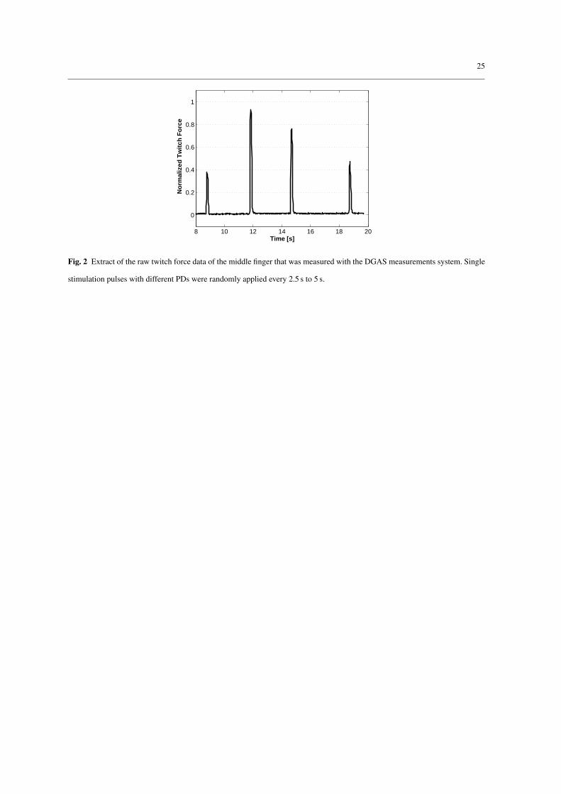
After a resting period of 1 min the isometric twitch forces of the middle finger were measured with the

dynamic grasp assessment system (DGAS) [20]. Single stimulation pulses with an amplitude of 20 mA and

with PDs of 0.05, 0.1, 0.3, 0.5, 0.7, 1, and 2 ms were randomly applied every 2.5 s to 5 s. Each PD was applied

a total of six times (randomized). An extract of the raw twitch force measurements is shown in Figure 2. Each

data series was normalized to its maximal value in order to obtain recruitment-duration curves.

2.3 Strength-duration curves, rheobase, and chronaxie

Rheobase Irh and chronaxie Tch from strength-duration curves calculated with the TES model were compared

with own experimentally obtained and previously published experimental rheobase and chronaxie values. In

the TES model strength-duration curves were obtained by calculating threshold currents Ith for PDs of 0.05,

0.1, 0.3, 0.5, 0.7, 1, and 2 ms. The threshold amplitudes were determined using bisection search with an

accuracy of 0.01 mA. At threshold only the thickest axon model closest to the electrode was activated (axon

diameter: 16 µm, depth: 0.6 cm). In the experiments motor thresholds were measured as described in section

2.2. Lapicque’s equation Ith = Irh/(1− exp(−PD/Tch)) [29] was fit to the measured strength-duration data in

order to obtain Irh and Tch. R-square (R2) values between the fitted curves and the actual strength-duration

data were calculated to check the accuracy of the fit (all values were below 0.8%).

8

2.4 Influence of tissue and stimulation parameters on chronaxie

The influence of tissue properties on the chronaxie was investigated in order to find out how the chronaxie

changes for different tissue thicknesses, tissue properties, electrode sizes, and nerve depths. The aim was to

investigate by computer modeling which parameters cause the large range of chronaxie values (200 - 700 µs)

observed in strength-duration measurements with surface electrodes (far-field situation).

Tissue thicknesses of the forearm model were changed in the range of values that cover most human

forearms [50, 45, 53]. The range of thicknesses was: for skin from 1 to 3 mm, fat from 2 to 30 mm, muscle

from 20 to 60 mm, cortical bone from 4 to 8 mm, and bone marrow from 4 to 8 mm. The range of resistivity

values that were tested are summarized in Table 1 (columns Min and Max) and cover the range of values that

can be expected in practical applications of TES [12, 45, 10, 40]. Electrode size was kept at 5cmx5cm when

changing tissue thicknesses and tissue properties. Afterwards, chronaxie values for electrode sizes between

0.1 cm x 0.1 cm and 7 cm x 7 cm and two nerve depths of 0.6 cm and 1.5 cm were calculated. Electrode sizes

below 0.5 cm x 0.5 cm are usually not used in TES and were included to allow a comparison of our simulated

chronaxie values with publications that use point sources as electrodes. The changes in chronaxie values were

calculated for all four nerve models (A to D).

2.5 Recruitment-duration curves and time constants

Simulated recruitment-duration curves were compared with experimentally obtained recruitment curves by

comparing the corresponding time constants τ [5]. The time constants τsim of the recruitment-duration curves

from the TES model were compared with the time constants τexp of the experimentally measured recruitment-

duration curves (twitch forces). Both time constants were calculated by fitting equation (3) to the recruitment

data as suggested in [5].

Rec = Recsat(1− e−(PD−PD0)/τ) f or PD > PD0 (3)

Rec = 0 f or PD < PD0 (4)

Rec is the recruitment, Recsat is the value where the recruitment saturates, PD represents the stimulation PD,

PD0 is the threshold PD above which an AP is generated, and τ is the time constant of the rising recruitment.

9

R-square (R2) values between the fitted curves and the actual recruitment data were calculated to check the

accuracy of the fit (all values were below 1.5%).

3 Results

3.1 Chronaxie of TES model

Chronaxie values (Tch) of the TES model were calculated from the simulated strength-duration curves depicted

in Fig. 3 (section 2.3). The calculated chronaxie values for the different nerve models are summarized in Table

2. The previously published chronaxie values that were obtained experimentally are shown in the same Table

2 and were determined for implantable systems where small electrodes were close to the nerve. For all nerve

models the chronaxie values of the TES model were higher compared to the published chronaxie values. The

chronaxie values using nerve models A, B, and D were in the range of experimentally obtained chronaxie

values for TES, which are between 200 µs and 700 µs [48, 15, 23]. The largest increase was found in nerve

model D, where the chronaxie increased by 205% from 150 µs to 457 µs. The values with nerve model C

(33 µs) were too short compared with the experimental range of 200 µs to 700 µs.

3.2 Influence of permittivities (capacitance)

The influence of the capacitive effects on Rec was investigated with the TES model using nerve model D.

The permittivities (εr) of electrode, skin, fat, and muscle were changed in the range of published experimental

values (Table 1). The results were produced for a stimulation pulse amplitude of 15 mA and a PD of 0.3 ms

(values that are commonly applied on forearms using TES). Permittivity changes at the electrode-skin inter-

face had no influence on Rec (<0.1%). Skin and fat permittivities changed Rec by 2%. The muscle permittivity

had the largest influence with 5%. Strength-duration and recruitment-duration curves were therefore calcu-

lated for the published range of muscle permittivities (Table 1) in order to identify an upper limit for the

influence of the capacitive effects.

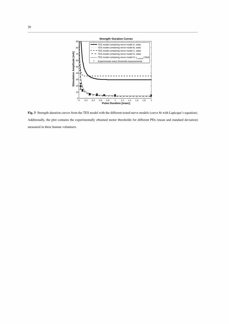
Increasing the muscle permittivity shifted the strength-duration to slightly higher values (Fig. 3). The

chronaxie was increased from 457 µs (static volume conductor) by 2% to 466 µs for εr = 1.2e5 and by 3.6%

10

to 474 µs for εr = 25e5. These changes are small compared to the large variations of chronaxie values in

experimental measurements of 200 µs to 700 µs [48, 15, 23].

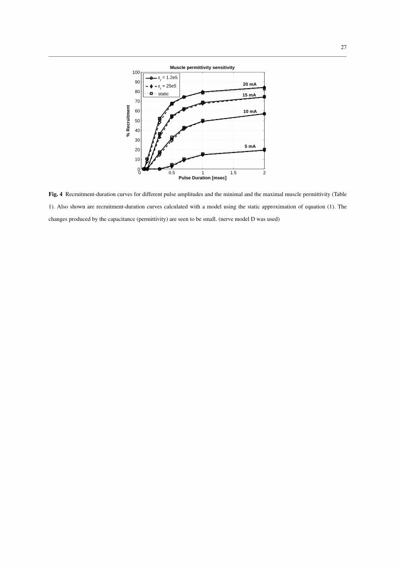
The recruitment-duration curves for the smallest and largest muscle permittivity are depicted in Fig. 4.

The curves show the percentage of axons that are activated in the nerve model for different pulse amplitudes

and durations. The influence on the time constants τsim was largest for small pulse amplitudes. At 5 mA

the time constant changed from 408 µs to 433 µs (6%) when increasing the permittivity from 1.2e5 to 25e5.

However, the changes in recruitment due to the capacitive effects of the muscle are small compared to changes

in recruitment caused by PD or pulse amplitude changes.

Fig. 4 also shows the recruitment-duration curve described by a model that uses a static approximation (ca-

pacitive effects of the electrode-skin interface and the bulk tissues neglected) of equation (1) for the FE model.

It can be seen that the curves are nearly congruent with the curves obtained using the model considering the

permittivities.

3.3 Influence of tissue and stimulation parameters on chronaxie

The influence of different tissue and stimulation parameters on the chronaxie was investigated. Changing the

tissue thicknesses and resistivities of the volume conductor model in the range of values that cover most human

forearms (see section 2.4) resulted in chronaxie changes below 1.1% for all four nerve models (percentage

was calculated relative to the chronaxie values in Table 2). Only the thickest fat layer (30 mm) had a larger

influence on the chronaxie (<6.3%). This is due to the spread of the current in the thicker fat layer that

influences more nodes of the nerve models simultaneously (see Discussion).

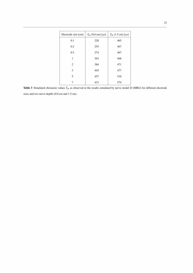
Changes of electrode size and nerve depth have a larger influence on the chronaxie. The results using nerve

model D are shown in Table 3 where it can be seen that the chronaxie values are in the range from 220 µs to

574 µs. In general, smaller electrodes and more superficial nerves result in smaller chronaxie values and vice

versa. For nerve models A to C smaller electrodes and superficial nerves also generated smaller chronaxie

values, however, the effect was less pronounced compared to nerve model D. The range of chronaxie values

was 124 µs to 171 µs using nerve model A, 112 µs to 149 µs using nerve model B, and 27 µs to 36 µs using

nerve model C.

11

3.4 Comparison of simulated with experimental strength-duration curves

The strength-duration curves that were calculated with the TES model containing the four tested nerve models

(A-D) were compared with experimentally obtained motor threshold amplitudes (mean and standard devia-

tion) for different PDs (see Fig. 3). The TES model with nerve model D matched best the experimental

measurements for all measured PDs. The thresholds obtained with nerve models A, B, and C were all at least

a factor of four higher. This was also indicated by the rheobasic currents (Table 2) that were too high for nerve

models A, B, and C compared to the experiments.

3.5 Comparison of simulated with experimental recruitment-duration curves

The time constants τsim (section 2.5) of the recruitment curves from the TES model were compared with

the time constants τexp of the experimentally obtained recruitment curves. The TES models including nerve

model A, B, or C used a current amplitude of 90 mA and the TES model with nerve model D used a current

amplitude of 20 mA. The current amplitude for models A, B, and C had to be increased due to the higher

rheobasic currents of these nerve models (Table 2).

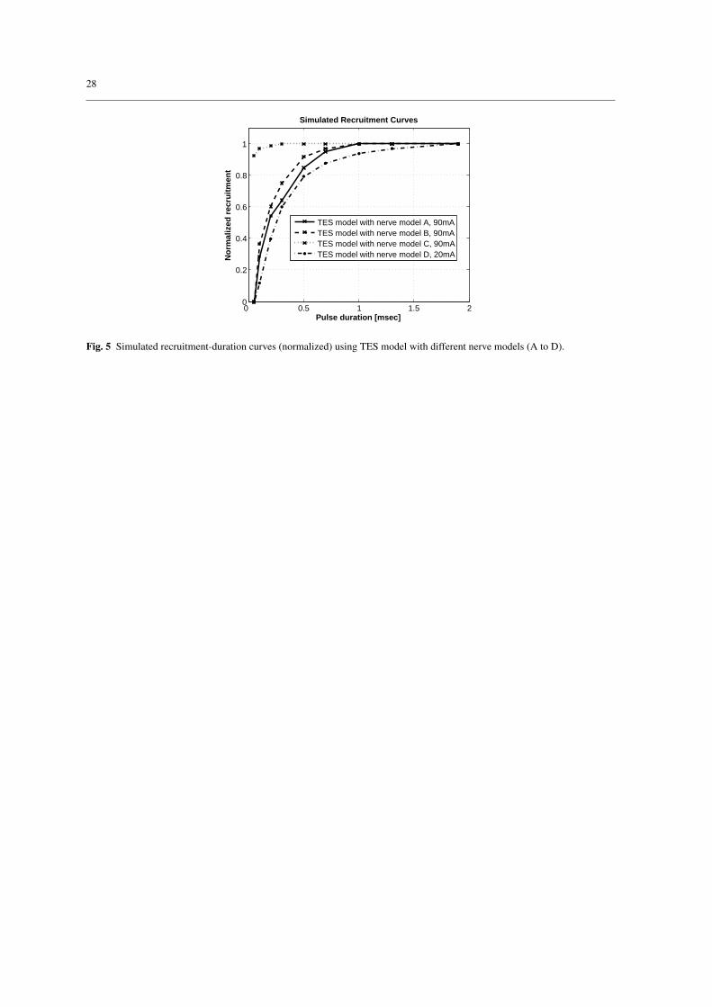
The normalized recruitment-duration curves obtained from simulations are shown in Fig. 5. The time

constants τsim were 189 µs with nerve model A, 164 µs with nerve model B, 19 µs with nerve model C, and

476 µs with nerve model D. The experimentally measured recruitment curves from the upper extremities are

shown in Fig. 6. The time constants τexp of these curves were 489 µs in volunteer one, 240 µs in volunteer

two, and 380 µs in volunteer three. The time constants τsim obtained with the TES model containing nerve

models A, B, or D were within the 95% confidence interval of the time constants τexp obtained by experimental

measurements. The value of τsim derived from using nerve model C was more than a factor of ten shorter than

the shortest τexp.

4 Discussion

We developed a two step model that describes the total dynamics from the applied stimulation current pulse

to nerve recruitment for TES. The model enabled us to find out if published nerve models that were used

in many studies for near-field stimulation with implantable electrodes are also suitable to describe far-field

12

stimulation (TES). This was unclear because of the large discrepancy between the chronaxie values of pub-

lished nerve models (30 µs and 150 µs) and chronaxie values obtained with surface electrodes (200 µs and

700 µs [48, 15, 23]). The simulation results in Table 2 show that the chronaxie values were increased when

using the tested nerve models in the TES model. The chronaxie values were increased up to 205% compared

with the chronaxie from publications, which were obtained with electrodes close to the axon. The capacitive

changes are not the reason for the increase as they had only a small influence (<6%). The results show that

the electrode sizes and the electrode/nerve distance have the largest influence on chronaxie values amongst

the tested parameters (Table 3). Smaller electrodes and smaller electrode/nerve distances resulted in smaller

chronaxie values. This was also found in studies that investigated implantable electrodes close to the axon

[44, 45]. Using different combinations of these two parameters in the TES model resulted in a range of 220 µs

to 574 µs when using nerve model D that described best the published experimental range (200 µs and 700 µs)

compared with the other tested nerve models (A to C). Possible reasons why nerve model D compared best

with experiments are discussed in section 4.1.

In order to find out how well the model describes TES, simulated strength-duration (Fig. 3) and recruitment-

duration curves (Figs. 5 and 6) were compared with experimental measurements. The cylindrical geometry

(tissue thicknesses), which we used (see Methods) was specified such that it compared well to intermediate

values of the three human volunteers (this was achieved using MRI scans in the same three human volun-

teers in an earlier study [27]). The results in Fig. 3 show that only the strength-duration curve using nerve

model D (MRG-model) compared well with the experiments. The rheobasic currents using nerve models A,

B, and C were too high. The recruitment-duration curves using nerve models A, B, and D compared well with

experiments. The reason why not all nerve models compared well with experimental data can be partially

explained due to different parameter values that were used in some nerve models (see section 4.1). Until now

the MRG-model was exclusively used for implanted ES systems [31]. With our investigations we could show

that the MRG-model can also be used to model transcutaneous ES where the electrode/nerve distances are

much larger than in implanted systems.

13

4.1 Parameter changes in used nerve models

It was investigated if changes in the parameters of nerve models A, B, and C can increase the chronaxie to

values found with nerve model D. The parameters from nerve model D that mainly influence the chronaxie

(membrane capacity, membrane resistivity, and axoplasm resistivity [44]) were applied to nerve models A,

B, and C. The chronaxie values of nerve models A, B, and C were at the most increased by 20%. Therefore,

most probably, the double cable structure, with explicit representation of the nodes of Ranvier, paranodal, and

internodal sections [37] was responsible for the longer chronaxie and not the different parameters of nerve

model D.

We showed that the TES models using nerve models A, B, or C had too high a rheobase (section 3.4 and

Fig. 3). The reason might be the different parameters of model D compared with models A, B, and C. The

nodal leakage conductance gL was 7mS/cm2 in D, but 30.3mS/cm2 in A and B, and 128mS/cm2 in C. The

axoplasmatic resistivity ρi was 70Ωcm in D instead of 110Ωcm in A and B, and 54.7Ωcm in C. Applying

the parameters from model D in model A and B lowered the thresholds at 0.2ms PD from 36 mA to 10 mA in

A and from 34 mA to 9 mA in B. These thresholds are closer to the experimentally obtained thresholds (see

Fig. 3) of 6.3 mA. Applying the parameters from model D in model C did not significantly change the motor

threshold found in the TES model containing nerve model C.

4.2 In which cases can the capacitive effects of the volume conductor be neglected?

The high variability of the electrode-skin interface and the published bulk tissue capacitances were found to

have a minor influence on recruitment in TES (Fig. 4). Therefore, the capacitive effects can be neglected,

which is equivalent to setting the time derivative term in equation (1) to zero yielding the Laplace equation.

However, the capacitive effects of the volume conductor have to be considered in the model for the following

cases:

- Investigations of time dependent voltage drops in the skin layer (which have a slow rise time): Such inves-

tigations are relevant if new pulse stimulation technologies, as for example presented in [19], are being

developed. For such cases a model considering the capacitive effects allows one to optimize the power

14

consumption because both the time dependent currents and the time dependent voltages can be simulated

(P(t) = U(t)∗ I(t)).

- Investigation of voltage regulated stimulation: It is important to note that only a simulation that incorporates

the tissues’ capacitance is able to produce reasonable values for the extracellular potential at the axon for

voltage regulated stimulation. The voltage drop in the skin layer increases over time because of the high

skin capacitance [7] and thus the extracellular potential at the nerve significantly drops during the applied

course of the pulse.

4.3 Spatial position of the nodes of ranvier

Axons with different diameters do not have the same internodal distance. As a consequence the nodes do

not lie at the same position underneath the electrode and could lead to different activation thresholds. To

investigate this we shifted the node of an axon by 0.1 mm steps within the internodal distance and could only

observe very small changes of the motor thresholds (<0.01mA). The reason that the shifts did not have an

influence was that the activation peaks were wider than the internodal distance.

4.4 Model limitations

The presented TES model has limitations that should be noted:

- In the presented TES model, nerve activation is calculated in two consecutive steps (FE model and nerve

model). The coupling between the two steps is established by interpolating the potential field calculated

using the FE model along the axons at Ve,n(t) (extracellular potential). This interpolation is discrete in

space and time which could introduce inaccuracies. The spatial interpolation is conducted at the axon

models’ nodes of Ranvier for axon models A-C. In nerve model D additionally an interpolation at the

paranodal and the internodal sections was performed. To ensure a good accuracy of this interpolation

the FE mesh size was refined until no significant change (<1%) was found in the resulting potential

distribution. The temporal interpolation was performed in 1µsec steps, which is much shorter than the PD

(> 50µsec in our model), helping to ensure numerical accuracy.

- The two calculation steps of the TES model (FE model and nerve model) are performed in one direction.

This means that the extracellular potential Ve,n(t) affects the axons’ TP, but the influence of the TP on

15

the extracellular potential is neglected. Both directions were taken into account for the first time in [36]

using a bidomain model. It was shown that the TP can influence the extracellular potential in direct muscle

stimulation, however, it was not shown if the generation of APs in adjacent muscle fibers is significantly

influenced. The method is computationally expensive and was therefore used on a simplified volume con-

ductor which was coupled with two muscle fibers [36]. Since, the presented TES model contains a more

detailed volume conductor and 1000 axons, the solution could currently not be computed in reasonable

time.

- The non-linear dependence of the bulk tissue properties to current density was neglected. This is not a major

concern as it was shown that with current-regulated pulses the non-linear properties of the bulk tissues can

be neglected [28].

- Dispersion of the bulk tissues was neglected. Sensitivity studies [25] showed that a wide range of tissue

properties did not influence neural activation. This indicates that dispersion can be neglected, too.

- The exact location where the APs are initiated in TES cannot be generalized due to geometrical and physi-

ological diversity. We accounted for that by using multiple nerve bundles at different depths.

5 Conclusion

A FE model was combined with previously published active nerve models to a TES model. The TES model

allows to describe the total dynamics from the applied stimulation current pulse to nerve recruitment and

serves as a tool to investigate the influences from the geometry, the tissue properties, and new stimulation

techniques.

For implantable stimulation (near-field) it was shown that mainly the electrode size and the electrode/nerve

distance influence the chronaxie. Our results show that the chronaxie is also in the far-field situation mainly

influenced by the electrode size and the electrode/nerve distance. With electrode sizes between (0.1 cm and

7 cm) and electrode/axon distances between 0.6 cm and 1.5 cm chronaxie values between 220 µs and 574 µs

were obtained. The capacitive effects, variations of the tissue resistivities, and variations of the tissue thick-

nesses have a minor influence.

Simulated strength-duration and recruitment-duration curves using the MRG-nerve-model (model D)

compared well with experimental measurements. We conclude from these results that the MRG-model can be

16

used with the same parameters for both implantable ES models and TES models. The parameters of the other

tested nerve models have to be adapted to compare well with experimental measurements.

With the presented TES model we developed a tool that should help to investigate and optimize new TES

technologies, such as multi-channel electrode arrays using non-uniform current distributions. It should help

to find appropriate designs for electrode geometries and stimulation pulse sequences.

Acknowledgements The project was supported by the Swiss National Science Foundation (SNF) No. 205321-107904/1.

References

1. Bajzek TJ, Jaeger RJ (1987) Characterization and control of muscle response to electrical stimulation.

Ann Biomed Eng 15:485–501

2. Baker LL, McNeal DR, Benton L, Bowman BR, Waters RL (2000) Neuro muscular electrical stimulation,

4th edn

3. Bostock H (1983) The strength-duration relationship for excitation of myelinated nerve: computed de-

pendence on membrane parameters. J Physiol 341:59–74

4. Chiu SY, Ritchie JM, Rogart RB, Stagg D (1979) A quantitative description of membrane currents in

rabbit myelinated nerve. J Physiol 292:149–66

5. Chou LW, Binder-Macleod SA (2007) The effects of stimulation frequency and fatigue on the force-

intensity relationship for human skeletal muscle. Clin Neurophysiol 118:1387–96

6. Crago PE, Peckham PH, Mortimer JT, Van der Meulen JP (1974) The choice of pulse duration for chronic

electrical stimulation via surface, nerve, and intramuscular electrodes. Ann Biomed Eng 2:252–64

7. Dorgan SJ, Reilly RB (1999) A model for human skin impedance during surface functional neuromuscu-

lar stimulation. IEEE Trans Rehabil Eng 7:341–8

8. Elsaify A, Fothergill J, Peasgood W (2004) A portable fes system incorporating an electrode array and

feedback sensors. In: Vienna Int. Workshop on Functional Electrostimulation, vol 8, pp 191–4

9. Fitzhugh R (1962) Computation of impulse initiation and saltatory conduction in a myelinated nerve fiber.

Biophys J 2:11–21

17

10. Foster KR, Schwan HP (1989) Dielectric properties of tissues and biological materials: a critical review.

Crit Rev Biomed Eng 17:25–104

11. Frankenhaeuser B, Huxley AF (1964) The action potential in the myelinated nerve fiber of xenopus laevis

as computed on the basis of voltage clamp data. J Physiol 171:302–15

12. Gabriel S, Lau RW, Gabriel C (1996) The dielectric properties of biological tissues: Iii. parametric models

for the dielectric spectrum of tissues. Phys Med Biol 41:2271–93

13. Geddes LA (2004) Accuracy limitations of chronaxie values. IEEE Trans Biomed Eng 51:176–81

14. Gregory CM, Dixon W, Bickel CS (2007) Impact of varying pulse frequency and duration on muscle

torque production and fatigue. Muscle Nerve 35:504–9

15. Harris R (1971) Chronaxy. In: S L (ed) Electrodiagnosis and Electromyography, Baltimore, pp 218–239

16. Hines ML, Carnevale NT (2001) Neuron: a tool for neuroscientists. Neuroscientist 7:123–35

17. Hodgkin AL, Huxley AF (1952) A quantitative description of membrane current and its application to

conduction and excitation in nerve. J Physiol 117:500–44

18. Holsheimer J, Wesselink WA (1997) Optimum electrode geometry for spinal cord stimulation: the narrow

bipole and tripole. Med Biol Eng Comput 35:493–7

19. Jezernik S, Morari M (2005) Energy-optimal electrical excitation of nerve fibers. IEEE Trans Biomed

Eng 52:740–3

20. Keller T, Popovic M, Amman M, Andereggen C, Dumont C (2000) A system for measuring finger forces

during grasping. In: International Functional Electrical Stimulation Society Conference, Aalborg, Den-

mark

21. Keller T, Popovic MR, Pappas IPI, Muller PY (2002) Transcutaneous functional electrical stimulator

"compex motion". Artificial Organs 26:219–223

22. Kesar T, Binder-Macleod S (2006) Effect of frequency and pulse duration on human muscle fatigue

during repetitive electrical stimulation. Exp Physiol 91:967–76

23. Kiernan MC, Burke D, Andersen KV, Bostock H (2000) Multiple measures of axonal excitability: a new

approach in clinical testing. Muscle Nerve 23:399–409

24. Kuhn A, Keller T (2005) A 3d transient model for transcutaneous functional electrical stimulation. In:

International Functional Electrical Stimulation Society Conference, Montreal, Canada, vol 10, pp 385–7

18

25. Kuhn A, Keller T (2006) The influence of capacitive properties on nerve activation in transcutaneous elec-

trical stimulation. In: International Symposium on Computer Methods in Biomechanics and Biomedical

Engineering, Antibes, France, vol 7

26. Kuhn A, Rauch GA, Keller T, Morari M, Dietz V (2005) A finite element model study to find the major

anatomical influences on transcutaneous electrical stimulation. In: ZNZ Symposium, Zurich, Switzerland

27. Kuhn A, Rauch GA, Panchaphongsaphak P, Keller T (2005) Using transient fe models to assess anatom-

ical influences on electrical stimulation. In: FEM Workshop, Ulm, Germany, vol 12

28. Kuhn A, Keller T, Prenaj B, Morari M (2006) The relevance of non-linear skin properties for a transcu-

taneous electrical stimulation model. In: International Functional Electrical Stimulation Society Confer-

ence, Zao, Japan, vol 11

29. Lapicque L (1907) Recherches quantitatives sur l’excitation electrique des nerfs traitee comme une po-

larisation. J Physiol Paris 9:622–35

30. Lawrence M, Pitschen G, Keller T, Kuhn A, Morari M (2008) Finger and wrist torque measurement

system for the evaluation of grasp performance with neuroprosthesis. Artif Organs in press

31. Lertmanorat Z, Gustafson KJ, Durand DM (2006) Electrode array for reversing the recruitment order of

peripheral nerve stimulation: experimental studies. Ann Biomed Eng 34:152–60

32. Livshitz LM, Einziger PD, Mizrahi J (2002) Rigorous green’s function formulation for transmembrane

potential induced along a 3-d infinite cylindrical cell. IEEE Trans Biomed Eng 49:1491–503

33. Manola L, Roelofsen BH, Holsheimer J, Marani E, Geelen J (2005) Modelling motor cortex stimulation

for chronic pain control: electrical potential field, activating functions and responses of simple nerve fibre

models. Med Biol Eng Comput 43:335–43

34. Martinek J, Reichel M, Rattay F, Mayr W (2004) Analysis of calculated electrical activation of denervated

muscle fibres in the human thigh. In: Proc. of 8th Vienna International Workshop on Functional Electrical

Stimulation, pp 228–31

35. Martinek J, Stickler Y, Dohnal F, Reichel M, Mayr W, Rattay F (2006) Simulation der funktionellen

elektrostimulation im menschlichen oberschenkel unter verwendung von femlab. In: Proceedings of the

COMSOL Users Conference 2006, Frankfurt, pp 20–23

19

36. Martinek J, Stickler Y, Reichel M, Rattay F (2007) A new approach to simulate hodgkin-huxley like exci-

tation with comsol multiphysics (femlab). In: Proc. of 9th Vienna International Workshop on Functional

Electrical Stimulation, pp 163–6

37. McIntyre CC, Richardson AG, Grill WM (2002) Modeling the excitability of mammalian nerve fibers:

influence of afterpotentials on the recovery cycle. J Neurophysiol 87:995–1006

38. McNeal DR (1976) Analysis of a model for excitation of myelinated nerve. IEEE Trans Biomed Eng

23:329–37

39. Mesin L, Merletti R (2008) Distribution of electrical stimulation current in a planar multilayer anisotropic

tissue. IEEE Trans Biomed Eng 55:660–70

40. Polk C, FL) CPBR (1986) CRC handbook of biological effects of electromagnetic fields. CRC Press,

Boca Raton - Fla.

41. Prodanov D, Feirabend HK (2007) Morphometric analysis of the fiber populations of the rat sciatic nerve,

its spinal roots, and its major branches. J Comp Neurol 503:85–100

42. Rattay F (1990) Electrical nerve stimulation theory, experiments and applications. Springer, Wien etc.

43. Reichel M, Martinek J, Mayr W, Rattay F (2004) Functional electrical stimulation of denervated skele-

tal muscle fibers in 3d human thigh - modeling and simulation. In: Proc. of 8th Vienna International

Workshop on Functional Electrical Stimulation, pp 44–7

44. Reilly JP, Bauer RH (1987) Application of a neuroelectric model to electrocutaneous sensory sensitivity:

parameter variation study. IEEE Trans Biomed Eng 34:752–4

45. Reilly JP, Antoni H, Chilbert MA, Sweeney JD (1998) Applied bioelectricity from electrical stimulation

to electropathology. Springer, New York etc.

46. Rijkhoff NJ, Holsheimer J, Koldewijn EL, Struijk JJ, van Kerrebroeck PE, Debruyne FM, Wijkstra H

(1994) Selective stimulation of sacral nerve roots for bladder control: a study by computer modeling.

IEEE Trans Biomed Eng 41:413–24

47. Schiefer MA, Triolo RJ, Tyler DJ (2008) A model of selective activation of the femoral nerve with a

flat interface nerve electrode for a lower extremity neuroprosthesis. IEEE Trans Neural Syst Rehabil Eng

16:195–204

20

48. Schuhfried O, Kollmann C, Paternostro-Sluga T (2005) Excitability of chronic hemiparetic muscles:

determination of chronaxie values and strength-duration curves and its implication in functional electrical

stimulation. IEEE Trans Neural Syst Rehabil Eng 13:105–9

49. Sotiropoulos SN, Steinmetz PN (2007) Assessing the direct effects of deep brain stimulation using em-

bedded axon models. J Neural Eng 4:107–19

50. Standring S (2005) Gray’s Anatomy, 39th edn

51. Strickler Y, Martinek J, Hofer C, Rattay F (2007) A finite element model of the electrically stimulated

human thigh: Changes due to denervation and training. In: Proc. of 9th Vienna International Workshop

on Functional Electrical Stimulation, Krems, Austria, pp 20–3

52. Sweeney J, Mortimer J, Durand D (1987) Modeling of mammalian myelinated nerve for functional neu-

romuscular stimulation. In: Proc. of IEEE 9th Annual Conference of the Engineering in Medicine and

Biology Society, pp 1577–8

53. Valentin J (2001) Basic anatomical and physiological data for use in radiological protection: reference

values. Annals of the ICRP

54. Vodovnik L, Crochetiere WJ, Reswick JB (1967) Control of a skeletal joint by electrical stimulation of

antagonists. Med Biol Eng 5:97–109

55. Zierhofer CM (2001) Analysis of a linear model for electrical stimulation of axons–critical remarks on

the "activating function concept". IEEE Trans Biomed Eng 48:173–84

21

Min Standard Max

Electrode interfaceρ [Ωm] 300

εr 1 1 2’000’000

Skinρ [Ωm] 500 700 6’000

εr 1’000 6’000 30’000

Fatρ [Ωm] 10 33 600

εr 1’500 25’000 50’000

Muscle ρ [Ωm] 2 3 5

(longitudinal) εr 100’000 120’000 2’500’000

Muscle ρ [Ωm] 6 9 15

(transverse) εr 33’000 40’000 830’000

Cortical boneρ [Ωm] 40 50 60

εr 3’000

Bone Marrowρ [Ωm] 10 12.5 15

εr 10’000

Table 1 Resistivities and relative permittivities of different tissues. Columns "Min" and "Max" are extreme values from [12, 45,

10, 40]. The column "Standard" contains properties used in an FE model that was verified with experimental measurements [24].

22

Nerve Axon Model Name Published Chronaxie Chronaxie Rheobase

Model ID Values in TES model in TES model

A Active Cable Model (FH) [38] 100 µs 157 µs 29.3mA

B Active Cable Temperature Comp. (FH) [42] p.86 100 µs 137 µs 29.2mA

C Active Mammalian Nerve (CRRSS) [4, 52] 26 µs 33 µs 35.1mA

D Active Double Cable (MRG model) [37] 150 µs 457 µs 2.97mA

Table 2 Comparison of published chronaxie values with chronaxie values obtained with the TES model (static volume conduc-

tor). Further, the rheobasic currents of the TES model for the different nerve models are given.

23

Electrode size [cm] Tch (0.6 cm) [µs] Tch (1.5 cm) [µs]

0.1 220 465

0.2 255 467

0.5 274 467

1 303 468

2 384 471

3 445 477

5 457 510

7 433 574

Table 3 Simulated chronaxie values Tch as observed in the results simulated by nerve model D (MRG) for different electrode

sizes and two nerve depths (0.6 cm and 1.5 cm).

24

Fig. 1 Schematic representation of the electrode-skin interface, the bulk tissues, and ten nerve bundles at depths between 0.6 cm

and 1.5 cm (from skin surface). On the bottom the electrical equivalent circuit of a myelinated axon. On the right the meshed

geometry of the arm model with surface electrodes (some tissue layers are partially removed for clarity). The model comprised

approximately 300’000 tetrahedral elements.

25

8 10 12 14 16 18 20

0

0.2

0.4

0.6

0.8

1

Time [s]

No

rmal

ized

Tw

itch

Fo

rce

Fig. 2 Extract of the raw twitch force data of the middle finger that was measured with the DGAS measurements system. Single

stimulation pulses with different PDs were randomly applied every 2.5 s to 5 s.

26

0 0.2 0.4 0.6 0.8 1 1.2 1.4 1.6 1.8 20

10

20

30

40

50

60

70

80

90

Pulse Duration [msec]

Stim

ulat

ion

Am

plitu

de [m

A]

Strength−Duration Curves

TES model containing nerve model A, staticTES model containing nerve model B, staticTES model containing nerve model C, staticTES model containing nerve model D, static

TES model containing nerve model D, εr,muscle=25e5

Experimental motor threshold measurements

Fig. 3 Strength-duration curves from the TES model with the different tested nerve models (curve fit with Lapicque’s equation).

Additionally, the plot contains the experimentally obtained motor thresholds for different PDs (mean and standard deviation)

measured in three human volunteers.

27

0 0.5 1 1.5 20

10

20

30

40

50

60

70

80

90

100

Pulse Duration [msec]

% R

ecru

itm

ent

Muscle permittivity sensitivity

ε

r = 1.2e5

εr = 25e5

static

20 mA

15 mA

10 mA

5 mA

Fig. 4 Recruitment-duration curves for different pulse amplitudes and the minimal and the maximal muscle permittivity (Table

1). Also shown are recruitment-duration curves calculated with a model using the static approximation of equation (1). The

changes produced by the capacitance (permittivity) are seen to be small. (nerve model D was used)

28

0 0.5 1 1.5 20

0.2

0.4

0.6

0.8

1

Pulse duration [msec]

No

rmal

ized

rec

ruit

men

t

Simulated Recruitment Curves

TES model with nerve model A, 90mATES model with nerve model B, 90mATES model with nerve model C, 90mATES model with nerve model D, 20mA

Fig. 5 Simulated recruitment-duration curves (normalized) using TES model with different nerve models (A to D).

29

0 0.5 1 1.5 20

0.2

0.4

0.6

0.8

1

Pulse Duration [msec]

No

rmal

ized

Tw

itch

Fo

rce

Experimental Recruitment Curves

Volunteer 1Volunteer 2Volunteer 3

Fig. 6 Recruitment-duration curves (normalized) of the middle finger from experimental measurements on three human volun-

teers. The stimulation amplitude was 20 mA.

30

Abbreviation Description

TES Transcutaneous electrical stimulation

AP Action potential

PD Pulse duration

FE Finite element

TP Transmembrane potential

VFE(t) Electric scalar potential

σ Conductivity

ρ Resistivity

εr Permittivity

Vn(t) Transmembrane potential at node n and time t

Ve,n(t) Extracellular potential at node n and time t

Ii,n(t) Ionic current at node n and time t

Cm Membrane capacitance

Ga Conductance of the axoplasm

Irh Rheobase

Tch Chronaxie

Ith Threshold current

τsim Time constant of simulated recruitment-duration curve

τexp Time constant of measured recruitment-duration curve

Rec Recruitment

Recsat Saturation value of recruitment

gL Nodal leakage conductance

ρi Axoplasmatic resistivity

Table 4 Abbreviations