Math1 Comput. Modelling Vol. 15, No. 2, pp. 59-75, 1991 Printed in Great Britain. All rights reserved

0895-7177/91 $3.00 + 0.00 Copyright@ 1991 Pergamon Press plc

A MODEL FOR THE CONVECTIVE COOLING OF ELECTRONIC COMPONENTS WITH

APPLICATION TO OPTIMAL PLACEMENT

B. CAHLON

Department of Mathematical Sciences, Oakland University Rochester, MI, 48309 USA

I. GERTSBAKH

Department of Mathematics and Computer Science, Ben Gurion University, Beersheva, Israel

I. E. SCHOCHETMAN AND M. SHILLOR

Department of Mathematical Sciences, Oakland University Rochester, MI, 48309 USA

(Received July 1990)

Communicated by Ervin Y. Rodin

Abstract-A mathematical model for the description of the evolution of temperature in a board of electronic devices is considered. The board consists of a grid with thermally active devices. These generate heat which is conducted to their neighbors and the edges of the board, as well as exchanged with a forced convective flow of cool air. The model consists of a discrete system of equations for the temperatures of the devices. Two versions of the model are presented, the cooling term being linear in one, and nonlinear in the other. Existence and uniqueness of solutions is proved for both models as well as convergence to the respective steady states. The model is used, in conjunction with the annealing algorithm, to find the optimal placement of electronic devices on a board in such a way as

to decrease the maximum temperature of the system.

1. INTRODUCTION

We present a mathematical model for describing the evolution of the temperature distribution in a planar device consisting of electronic components under convective cooling. Each of the components generates heat which is conducted to its neighbors or carried away by a stream of cool air. Our model is intended to be used in studies on the optimal placement of such components, since their thermal reliability depends on their temperatures which, in turn, depend on their placement. We analyze linear and nonlinear versions of the model and prove the existence of a unique solution in each case. We also show that the solution of each time dependent problem converges to the unique solution of the steady state problem. Finally, we consider an example where the annealing algorithm is used to find the optimal placement of the components on a grid so that the maximum temperature in the system is minimized.

The failure rates of most electronic components depend on their temperatures. For example, this dependence may involve the maximum temperature, a temperature threshold or the rate of change. Thus, the performance and reliability of boards with electronic devices may depend essentially on the way these devices interact thermally and therefore on their placement. In order to investigate the reliability of such systems, a model is required which accurately describes the evolution of temperature in the system.

Component placement optimization has been considered in the engineering literature (see e.g., Dancer and Pecht [l], Steinberg [2], H anneman [3], Osterman and Pecht [4] and references therein). Since the main interest has been reliability, more emphasis was directed to failure rates than to the detailed modeling of the heat conduction process. Indeed, Dancer and Pecht [l]

The authors would like to thank D. Schmidt and S. Shi for helpful discussions.

Typeset by A@-QX

59

60 B. CAHLON et al.

consider a simplified situation of a board consisting of one row of devices, each of which interacts only with a slow air flow, with no heat conduction taking place among the neighboring devices.

A more realistic model was considered by Gertsbakh [5] where heat conduction was taken into account, as well as heat exchange with a cooling stream of air. Although the model is two dimensional, attention is restricted to the steady state problem.

We use a generalization of the model in [5] for the description of the temperature evolution of a board with interconnected electronic components. The model describes a two dimensional (planar) grid whose electronic components: (1) interact thermally with each of their neighbors via heat conduction, (2) act as sources of heat and (3) exchange heat with an air current. Once the initial and boundary temperatures of the board are specified, we are able to solve for the temperature of each component as it evolves in time, using a discretized (in time) marching process. This is a considerable generalization of the model in [l].

Although our model is of interest in its own right, it can, for example, be used to study the optimal placement of electronic devices for the purpose of increasing the reliability of such systems. The goal is to minimize some objective function, which depends on the temperature and which is related to the failure rate. The simplest such objective function is the maximum temperature, at all time intervals, of all the devices. It is known (see e.g., [l] and the literature therein) that even a decrease of a few degrees in the maximum temperature can increase the reliability considerably, especially when Arrhenius-type failure rates are used.

Since the maximum temperature is to be minimized, it is clear that when the evolution of the temperature in the system is monotone, i.e., at each node the temperature is nondecreasing with time, only the steady state is of interest. Indeed, the highest temperature in this state is the highest for the whole evolution process. On the other hand, especially in nonlinear problems, the transient behavior may be very important if there is a considerable temperature increase initially. Moreover, in the case of nonlinear cooling, in order to compute the steady state, one has to use some iteration method. An obvious choice here is to use the time dependent process as an iteration scheme. In this way, one obtains relevant information about the temperature evolution as well.

The use of the model for optimal placement of electronic devices with respect to thermal failure rates is very simple. For a given arrangement of the components on the board, one solves the heat conduction problem and computes the maximum temperature at any location at any time. Then two components are interchanged and the maximum temperature is computed again from the model. A deterministic process would result if all possible permutations were considered, in which case any minimum configuration for the maximum temperature would be chosen. The drawback is the prohibitive amount of computing necessary for this approach. An alternative approach is to use the annealing algorithm which was introduced by Metropolis el al. [6] and applied to optimization problems by Kirkpatrick et al. [7] and Cerny [S] (see also [9]). The convergence of the algorithm was considered in [9], where a clear explanation of the subject can be found.

In our problem, the annealing algorithm is applied as follows. The maximum temperature Ti is computed for the current configuration of the devices. A new configuration is obtained from the current one by the interchange of a pair of devices. The maximum temperature Tf of the new configuration is computed and compared with Ti. If lower, the new configuration becomes the current configuration, Tf is set to Ti, and another pair of devices is exchanged. If Tf > Ti, it still may be accepted as the current configuration with some probability which depends on Tf - Ti. This probabilistic acceptance of a higher state is motivated by the desire to have the process not end at a relatively high local minimum. This approach provides a mechanism for escaping from such minima.

Our mathematical model is developed in Section 2, where the various assumptions are presented and the general equations derived. The linear version of the model is considered in Section 3, where we prove the existence of a unique steady state, construct it and then show that the time marching process converges to this state. The nonlinear case is considered in Section 4, where we prove existence, uniqueness and convergence of the time matching process. Finally, in Section 5 we use the annealing algorithm in conjunction with the model to find the optimal placement of components in an example.

A model for the convective cooling 61

2. THE GENERAL PROBLEM

In this section, we describe a model for the determination of the time evolution of the tem- perature field in a thermeresistive network consisting of a board with interconnected electronic components. As a result of the electric currents in the system, each electronic element generates heat which is conducted to its directly linked neighbors and, in part, is carried away by heat exchange with a convective air flow. Heat balance at each element or component relates the tem- perature increase to the heat generation in the element, the heat conductance to other elements and the cooling effect of the convective flow.

We use a discretized version of the heat equation to obtain an algebraic system, the solution of which represents the temperature of each of the elements. It is assumed that each component in the system possesses a uniform temperature at a given time instant, which seems reasonable when the elements are not too large.

We turn to the mathematical model for the process. Consider a rectangular board in the form of a grid such that each grid point or node (i, j) represents an electronic device. Let

G = {(i,j); i=O,l,..., I+1 and j=O,l,..., J+l} (2.1)

be the representation of the grid. There are IJ internal nodes which represent the components while the nodes on the edges of G represent the interaction of the board with other parts of the system. These are considered below.

If T = T(z, y, t) is the temperature at time t at point (2, y) of the device, we set

T$’ = T(iAx, jAy, mAt),

where At is the time step, while Ax and Ay are the grid steps in the I and y directions, respectively. We have, by (2.1), that 0 < a’ < I + 1, 0 5 j 5 J + 1 and m = 0, 1,2, . . . . Let Pij be the rate of heat production of the element at the node (i, j), and let &j and &j be the thermal conductances between the node (i, j) and the nodes (i- 1, j) and (i, j - l), respectively. If T, > 0

is the ambient temperature of the air flow, the rate of cooling of element (i, j) is assumed to be

kj (Ta-T) IT,--q 17-1, (2.2)

where the &j are the (positive) heat exchange coefficients and y 1 1 is the cooling exponent. When 7 = 1, this term is linear and consequently the problem is linear. It is considered in Section 3. When y > 1 the problem is nonlinear; it seems from the literature (see e.g., [2, 51) that 7 = 5/4 is a reasonable choice. The nonlinear problem is considered in Section 4. Notice that when an element’s temperature is greater than the ambient temperature, i.e., T > T,, the term in (2.2) is negative, that is, the element is being cooled. When its temperature is below, i.e., Tiy < T,,

the term is positive, and therefore, it is being heated. We consider the heat balance at a typical interior node (i, j). The rate of temperature increase

can be written, at time t = mAt, as

where the heat flow between adjacent elements is proportional to their temperature difference and c is the specific heat, assumed a constant. We use a forward finite difference approximation

62 B. CAHLON ef al.

in (2.3). Next, we introduce the notation

aij = ziij/c, bij = &ij /c 9 Pij = Fij/c and .&j = %j/c, (Z-4)

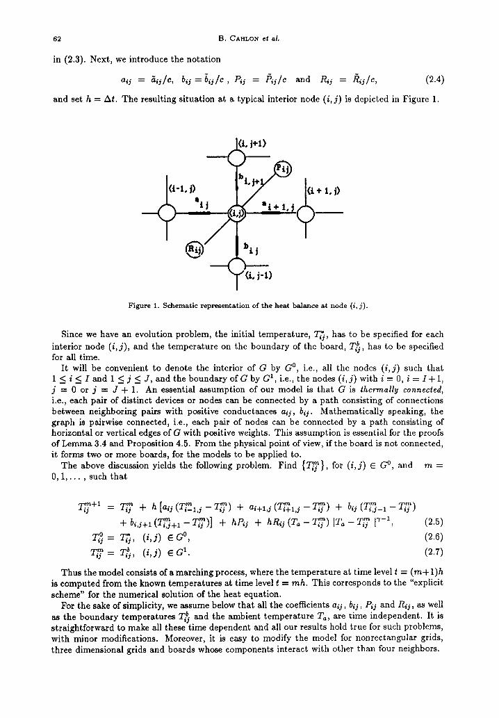
and set h = At. The resulting situation at a typical interior node (i, j) is depicted in Figure 1.

Figure 1. Schematic representation of the heat balance at node (i, j).

Since we have an evolution problem, the initial temperature, TG, has to be specified for each

interior node (i,j), and the temperature on the boundary of the board, T&, has to be specified for all time.

It will be convenient to denote the interior of G by Go, i.e., all the nodes (i, j) such that 1 5 i 5 I and 1 2 j 5 J, and the boundary of G by G1, i.e., the nodes (i, j) with i = 0, i = I+ 1, j = 0 or j = J + 1. An essential assumption of our model is that G is thermally connected,

i.e., each pair of distinct devices or nodes can be connected by a path consisting of connections between neighboring pairs with positive conductances aij, bij. Mathematically speaking, the graph is pairwise connected, i.e., each pair of nodes can be connected by a path consisting of horizontal or vertical edges of G with positive weights. This assumption is essential for the proofs of Lemma 3.4 and Proposition 4.5. Prom the physical point of view, if the board is not connected, it forms two or more boards, for the models to be applied to.

The above discussion yields the following problem. Find {Tin}, for (i, j) E Go, and m =

0, 1,. . . ) such that

T+’ = T + h [aij (Ti’!l,j -Tiy) + ai+l,j (y+l,j -I$‘) + bij (Tiz_1 -Tir)

+ bi,j+l (!$+I - Tr)] + hPij + h&j (Ta - !i$y) ITa - qy I-‘-l, (2.5)

T; = q;, (i,j) E Go, (2.6)

T; = Z$, (i,j) E G1. (2.7)

Thus the model consists of a marching process, where the temperature at time level t = (m+l)h is computed from the known temperatures at time level t = mh. This corresponds to the “explicit

scheme” for the numerical solution of the heat equation. For the sake of simplicity, we assume below that all the coefficients aij , bij , Pij and Rij, as well

as the boundary temperatures Th and the ambient temperature T,, are time independent. It is straightforward to make all these time dependent and all our results hold true for such problems, with minor modifications. Moreover, it is easy to modify the model for nonrectangular grids, three dimensional grids and boards whose components interact with other than four neighbors.

A model for the convective cooling 63

As was mentioned in the introduction, the model describes the spatial and temporal evolution of the temperature. It is well known that in the limit as h = At --+ 0, Ax + 0 and Ay --+ 0, (2.5) reduces to the heat equation

g = ;(ag) + $(bg) + P+ R(T,-T)IT,-TIT-1,

where a, b, P and R are the appropriate limit function coefficients.

3. THE LINEAR MODEL

In this section we consider the linear version of our model, i.e., the csse where y = 1. First, we prove the existence of a unique steady state and give an explicit representation of it. Then, we show that the sequence of solutions to (2.5)-(2.7) converges to the steady state solution.

A 2,

We define

Cij = aij + ai+l,j + bij + h,j+l, (i, j) E Go.

Then the linear problem (2.5)-(2.7), with y = 1, consists of finding {y}, m = 0, that

T+l = (1 -&j)Tt + h [oijri,j +oi+l,j 7$i,j + bij ‘&;_I +

+ bi,j+l %+I] + h [Pij + &j (7’a -q)] 7 (GA E Go,

together with the initial and boundary conditions

T; = T;, (i, j) E Go,

T = T;, (i, j) E G’.

(3.1) , such

(3.2)

(3.3)

(3.4)

The model (3.2)-(3.4) g enerates a sequence of temperature distributions on G. We next consider conditions on the data which guarantee the existence of a steady state temperature distribution. Then we shall discuss how to find it and show that the sequence generated in (3.2)-(3.4) converges to the steady state solution.

It is convenient to represent the problem in vector form. To this end, let K = IJ and, for k= l,...K,let

k = i + (j - 1) I, (i, j) E Go. (3.5)

This is an enumeration of the interior nodes by a single index k instead of (i, j), yielding a one- to-one correspondence. We start at the bottom left and proceed from left to right and bottom to top. We shall write k * (i, j) to denote this correspondence. For m = 0, 1, . . . , we set

tm - 2? k- ‘3 ’ fk = Rij, Pk = pij, t; = T;, k ++ (i j) E Go. (3.6)

Also, let

tm = (ty, . . . , tz), p = (pi,. . . ,p~), r = (PI,. . . , TK), t* = (t;, . . . , t>).

Next, we construct the I< x I< matrix B = (&l) as follows:

(i) k t+ (1, l), i.e., k = 1,

&I = Cll, Bk2 = -a21, &,I+1 = -h2,

Bkl = 0, otherwise;

(3.7)

(ii) k t+ (i, l), 2 5 i 2 I - 1, i.e., k = i,

&,i-1 = -ail, Bki = Gil,

MCM 15:2-E Bkt = 0, otherwise;

Bk,i+l = -ai+l,l, &,I+ = -biz,

64

(iii) k * (I, l), i.e., k = I,

B. CAHLON et al.

&,I-1 = -all, &I = CII,

Bkl = 0, otherwise;

&,z = -bn,

(iv) k * (1, j), 2 5 j 5 J - 1, i.e., k = 1 + (j - 1) I,

Bk,(j-2)1+1 = -hj, Bk,(j-l)z+l = Clj, Bk,(j-l)z+2 = -%j,

Bk,jz+l = - b l,j+l, Bkl = 0, otherwise;

(v) k * (i,j), 2 5 i 2 I - 1, 2 5 j 5 J - 1, i.e., t = i + (j - 1)1,

-bij 9 e = (j - 2) I + i,

-atj, fJ=(j-1)1+i-1,

&l = I Cij 3 e = (j - 1) I + i,

-ai+l,j, !!=(j-1)1+i+1,

-b. . w+17 e=jr+i,

0, otherwise;

(vi) k +-+ (I,j), 2 5 j 5 J - 1, i.e., k = I + (j - 1)1 = j1,

Bk,G-l)z = -b,, Bt,jI-1 = -arj, Bk,jr = Crj 9 Bk,(j+l)z = -bI,j+l, Bkf = 0, otherwise;

(vii) k * (1, J), i.e., k = 1 + (J - 1) I,

&,(J-2)ztl = -hJ, &,(J--1)z+l = CIJ, &,(J-qz+2 = -2J,

Bkt = 0, otherwise;

(viii) k * (i, J), 2 5 i 5 I - 1, i.e., k = i + (J - 1) I,

Bk,(J-s)z+i = -bi.z, Bk,(J-i)z+i-1 = -ad,

&,(J-1)ztitl = -%tl,J, Bk,l = 0, otherwise;

(ix) k ++ (I, J), i.e., k = I+ (J - 1) I = J I,

Bk,(J-1)z = -bzJ, &,zJ-1 = -aZJ,

Bkt = 0, otherwise.

&,(J--l)l+i = ‘%J,

B k,IJ = CZJ,

Notice that (v) d escribes the interior nodes while the rest describe nodes near the boundary of the board.

We use the following notation. If x = ($1,. . . ,ZK) E RK then D(x) denotes the diagonal

matrix (&) such that

Dij = “d” i = j,

> otherwise.

Let E be the K x K identity matrix and set

C=E-hB,

where B is the matrix constructed above.

(3.8)

A model for the convective cooling 65

In order to state the linear problem (3.2)-(3.4) in vector form we need the boundary data vector v = (VI,. . . , UK), defined as

vk =

k - (1, l), k CI (i, l), 2 < i 5 I - 1,

k ++ (I, l),

k * (l,j), 2 5 j 5 J - 1,

k++(i,j),2<i<I-1,25jsJ-l, (3.9)

k - (I,j), 2 6 j 5 J - 1,

k ++ (1, J),

k ++ (i, J), 2 5 i 5 I - 1,

k c* (I, .7).

Notice that vk > 0 for k = 1,. . . , K. Finally, let

H=E-hB-hD(r). (3.10)

Using (3.7)-(3.10) we rewrite (3.2)-(3.4) as follows. Find {t”} , m = 1,2,. . . , such that

tm+l = H tm + h (v + p + T, r) and to = t*. (3.11)

The main result of this section is the following.

THEOREM 3.1. Assume that h > 0 is sufficiently small. Then the sequence {tm}~=o constructed in (3.11) converges, as m + co, to the unique steady state solution

tm =(B+D(r))-‘(v+p+T,r). (3.12)

The proof is given below following some intermediate results. The restriction on h is given explicitly in (3.14).

REMARK 3.2. It is easy to see that (3.12) is a solution to the steady state problem

(B + D(r)) t = (v + p + T, r),

obtained from (3.11) by formally taking t = tm+l = t”‘.

(3.13)

We shall need the following properties of the matrix H = (Hkl).

LEMMA 3.3. Assume that

0 < h I CjzyG,,{(cij + Rij)-‘}a

Then:

(3.14)

(i) Hkk = 1 - h (Cij + I&j), k * (i, j) E Go;

(ii) O<Hkk<l, O<Hkt, k,l=1,2 ,..., I<;

(iii) 2 Hkd 2 1, k +-+ (i,j) E Go; Ccl

(iv) 5 Hkc = l-h&j, k ++ (i,j), 2 5 i 5 I - 1, 2 5 j 5 J - 1. L=l

(3.15)

(3.16)

(3.17)

(3.18)

66 B. CAHLON et al.

PROOF. This is a straightforward consequence of the construction of B and H. We may rewrite the problem (3.11) in the form

tm+l =H”‘tO+h gHn ( )

(v + P+ Tar), m= 1,2,... . r&=0

(3.19)

In order to determine the convergence properties of the marching scheme (3.19), we investigate conditions for H to be a convergent matrix, i.e., such that

H”+O and FHn --) (E-H)-‘, as m-+oo, (3.20) n=O

the convergence being componentwise.

LEMMA 3.4. Assume that h satisfies (3.14). Then the spectral radius o(H) of H is strictly less than 1. Consequently, H is a convergent matrix.

PROOF. Recall, from [lo], that

a(H) = max{]X]; )r is an eigenvalue of H).

For each k = 1,. . . K, and C the complex numbers, define the circle

and let kl

2 = i, Zk. k=l

By the Gershgorin Circle Theorem [lo, p. 471, if X is an eigenvalue of H, then X E Z. By Lemma 3.3, for each k c-+ (i,j) E Go, 0 5 Hkk < 1 and

Hkk + 5 fikL 5 1. t=1 t#*

Hence, each circle Zk lies in the (closed) unit circle and so Z is there, too. Thus, it remains to show that 1 is not an eigenvalue of H.

We argue by contradiction. Suppose that 1 is an eigenvalue of H. Then there exists w E RK,w # 0 such that Hw = w, i.e., (E - H)w = 0. But H = E - hB - hD(r), by (3.10), so (B + D(r)) w = 0, i.e., B + D(r) is a singular matrix. Since Go is thermally connected, matrix B has property SC (see [ll , 6.271). H ence, B + D(r) also has property SC and is strictly diagonally dominant. Consequently, B + D(r) is nonsingular [ll, 6.1.101, a contradiction. Thus, 1 is not an eigenvalue and so, a(H) < 1.

We are in position now, to prove the theorem.

PROOF (OF THEOREM 3.1). Form= 1,2...,

tm+l _ Hmto = h

by (3.19). Since H is a convergent matrix (3.20), it follows that

lim tm+’ = h(E-H)-‘(v+p+T,r), t-em

that is, tw = (B + D(r))-‘(v + p + T, r).

Thus, the theorem holds as long as h satisfies (3.14). Notice that B represents the thermal properties of the grid or board, r the convective properties

and v the boundary temperatures. Thus, the steady state solution reflects the interaction with the environment of the system and the heat generating properties of the elements, as well as their placement on the grid.

A model for the convective cooling 67

4. THE NONLINEAR MODEL

In this section, we consider the full nonlinear model, i.e., the case where 7 > 1. We prove that the sequence generated by the time marching process converges to the unique steady state solution of the problem. Since the model is nonlinear, both the convergence and the existence of a unique steady state are not trivial or straightforward.

In order to rewrite (2.5)-(2.7) in vector form, let t, = (T,, . , . , T,) and define

t; = (It? -&I+,... ,It;)-Talr-l), m=0,1,2 ,... .

Then, using the notation of Section 3, we may write the problem as follows. Find {tm}~=o c RK such that

(4.1)

tm+’ = C tm f h (v + p) - h D(r) D(t” - to) ty, (4.2)

and to = t*. (4.3)

The initial and boundary temperatures are assumed to be specified as in the linear model. The scheme (4.2) and (4.3) represents a time marching process and our main concern is to show that as t -+ 00, i.e., as m ---, 00 (with h > 0 fixed), the process converges to the steady state solution. To this end, we introduce the mapping F : RK + RK given by

F(x)=Cx+h(vfp)-hD(r)D(x-&)x7, XERK, (4.4)

where xY = _ $zr; 2!-‘9 * * * 9 IZK - Tajrel), as in (4.1). If we write F = (Fl, . . . , FK), then Fk:RK , , . . . Ii, where

K

Fk(x) = c CkC XL + h (vk + pk) - h rk (2k - Ta) 1zk - Ta17-l,

kl

x E RK. (4.5)

For convenience, we slightly abuse notation and write xij interchangeably with zk for k = i + (j - l)I, (i,j) E Go. U sing (4.4), problem (4.2)-(4.3) may be written as follows.

Find {tm}~=o c RK such that

tm+’ = F(tm), m= 1,2,... , to = t*. (4.6)

Our main result in this section is the following.

THEOREM 4.1. Assume that h > 0 is suficiently small. Then:

(i) the sequence {tm},“,o generated in (4.4) is contained in a bounded subset X c RK, which depends on the data only;

(ii) the mapping F satisties F(X) c X and has a unique fixed point in X; (iii) this fixed point is the unique steady state solution to the nonlinear problem.

The proof of the theorem is given in several steps.

LEMMA 4.2. The mapping F is fiecbet differentiable everywhere and the derivative F’(x) is given by

F’(x) = C - h 7 D(r) D(x,), XERK. (4.7)

PROOF. It is known that F’(x) is equal to the Jacobian matrix dF/dx of F, [ll, p. 1711. Moreover,

aF *[Cx+h(v+p)-hD(r)D(x-&)x7]

z-c= 8x

= C-hD(r) ; [D(x - t(l) xr]

= C - hyD(r) D(x?), 2 E RK.

68 B. CAHLON et al.

Our next objective X c RK into itself.

is to show that for h > 0 sufficiently small, F maps an appropriate rectangle

Let

b = (i.lyG,, {l~j I, lbij 11.

Then b > 0, since G is thermally connected by assumption. Let

(4.8)

(4.9)

so that 0 5 r+ _< r*. We assume

0 < r,.

This assumption, which is physically reasonable, is crucial to the proofs below. Next, let N > 0 be such that

(4.10)

O<T; <N, (4d E Go, (4.11)

and

Define

p’ = max {pij}.

(i,j)EGO (4.12)

(4.13)

Clearly p > 2. We let

so that N < M and also

Finally, we define X c RX by

M = PTn, (4.14)

llY 5 M. (4.15)

X = {XE RK; 0 5 xk 5 M, 1 5 k 5 Ii-}.

Trivally, X is a convex, compact, connected subset of RK.

(4.16)

PROPOSITION 4.3. Assume that h > 0 is sufficiently small. Then

F(X) 5 X. (4.17)

PROOF. It is enough to show that 0 5 F’j(x) 2 M, for all (i,j) E Go and x E X. Fix (i,j) E Go and let x E X, i.e., 0 < 2kt 5 M, all (k,!) E Go. For arbitrary 6 > 0, define A = p’/T, > 0 and let

hI =

hz =

hs =

h4 =

and

1-6

4bP+X > 0,

1

4bp+X+r*z-l > 0,

b

r* (p - 2)7 c-l ’ O’

s

r* (p - 1)7-l z-’ ’ O’

h = min{hi, ha, hs, h4). (4.18)

A model for the convective cooling 69

It is easy to verify that 0 < 6 < 1 - h cij < 1, all (i, j) E Go. We divide the proof into three cases:

(1) 0 I Xij 5 T,, (2) !I’, < xii < (P - 1) Z’, and (3) (P - 1) T, 5 xii 5 M. Case (1). Assume 0 5 rij 5 To. Then it follows from (4.5), using (4.8)-(4.13) and (4.18), that

Fij(X)l (1shcij)Ta+hCijM+hp*+hr* lzij-T,I’

5 T,+h [4bM+p*+r*c]

I T,+h[4bp+A+r*q-‘IT,

= T, 1,; [ 1 <2T,<M.

The requirement 0 5 Fij(x) follows from the fact that x ij 5 Ta. Hence, all the terms in (4.5) are positive.

Case (2). Assume T, < xij < (p - 1) T,. Then

Fij (X) 1 (1 - h cij) xij - h R+j(xij - To) I~ij - T, 17-l

> (l-hCij)T,-hr*(p-2)‘~

3 [6 - h r*(p - 2)7 csl] T,

= 6 (1 - h/ha) T, 2 0,

where the last inequality follows from the definition of h3 above. In the other direction, we have

&j(X) I (l_hcij)(p_l)T,+4hbM+hp*

< (P-l)T,+h[4bM+p*]

= (P-l)T,+h[4bp+X]T,

S[(P-l)+h1(4bp+X)]T,

= (P-6)T, <PT,=M.

Case (3). Finally, assume (/3 - 1) T, 5 Zij 5 M. Then

fij(x) <M+hp*-hr,(P-2)‘2-;7

SM+h[p’--r,(p--2)rq] <M,

where the term in the brackets is nonpositive, since by (4.13)

i.e.,

r.*c(P-2)7 2 p’.

In the other direction, we have

Fij(x) 1 (1shcij) (P-l)Ta-hr*(M-T,)’

>_ S(p- l)T, - hr*(p-- l)‘c

L (P - 1) Tc, 6 [l - h/ha] 2 0.

This concludes the proof of the proposition.

We next turn our attention to the matrix C of (3.8). We have the following analogues of results in Section 3.

LEMMA 4.4. Assume that

(4.19)

70 B. CAHLON et al.

Then the matrix C = (GkL) has the following properties: (j) the diagonal is given by

ckk = l- hcij, k ++ (i,j) E Go;

(jj)CkL2OilIldOICkk<l,foraJ1k,e=1,2 ,... K; (iii) for each k ++ (i,j) E Go, such that 2 5 i 5 I - 1, 2 5 j 5 J - 1,

K

c ckl = 1; kl

(iv) for each k * (i, j) E Go other than those in (iii),

kl

PROOF. The proof is straightforward and consists of writing out the entries explicitly. In order to investigate the convergence properties of the scheme (4.6) we need the following.

PROPOSITION 4.5. Suppose that h satisfies (4.19). Then the spectral radius a(C) of C satisfies

u(C) < 1. (4.20)

Hence, C is a convergent matrix.

PROOF. The proof follows that of Lemma 3.4.

LEMMA 4.6. Let 7 = i(l - u(C)) > 0. Then there exists a vector norm I] . ]I on RK such that, for the corresponding matrix norm, we have

that is l]C]] < 1.

IICII 5 4C) + ‘7, (4.21)

PROOF. Follows from [lo, 1.3.6.1. In what follows, we shall need a description of this vector norm. Let P be an invertible matrix

such that P-‘CP is the Jordan form of C. Let D, be the K x K diagonal matrix with diagonal (1,q . . . ,eK-1 ), for 6 > 0. Then for each x E R K, the norm in Lemma 4.6 is given by

lkll = II&t J&9

where I] . Ilo3 is the too norm and Qc = (PD,)-‘.

(4.22)

PROPOSITION 4.7. For sufficiently small h > 0, there exists 0 < [ < 1 such that

P’WII I t, x E x. (4.23)

PROOF. For x E X, we have

1 llcll - IlF’Wll 1 5 IIF’W - Cl1 = 7h]]D(r) D(xr)]]

A model for the convective cooling 71

by Lemma 4.2. Then

ID(r) D(x7)ll =

=

,;yl II%) D(xr) 41

,,QTyuyw=l IIQ? W’W+ll~

,,qy~~, IIQr’W W,) Qawlloo

,,w?l;F_I IIDT’P-‘w D(J5)PD~ wllw

+%o(P) r* IID(xr)llm,

where llDclloo = 1, llD;‘lloo = 61-K (since 0 < E < 1) and K~(P) is the condition number [[P-1\\, llPlloo of the matrix P in the k’O”-norm. Thus,

1 IICII - llF’(x)II I I ~hc’-~ b(P)r* IID(x,)ll~~ x E x.

But x E X implies lzk - T,I 5 M, 1 5 k 5 K, so that

llD(4llca I MT-‘,

i.e., 1 II CII - llF’(x)ll 1 5 +‘-K K~(P) r*Mr-‘, x E X.

Let t = a(C) + 277, so that 0 < [ < 1 and IlCll < <. Choose h > 0 such that

h< t - IICII y cl-G,(P) r*kfr-1 *

(4.24)

Then IIF’(x)ll 5 llCl[ + 7 h?K G,(P) r*My-’ 5 <,

and the proof is complete.

x E x,

COROLLARY 4.8. The restriction of F to X is a contraction with respect to the norm II e 11.

PROOF. Let x, y E X. Then [12, 8.4.51

IIF - F(Y)11 5 ocp,l IIF’((1 - e>x + eY>ll IIX - YII 5 e IIX - Yll, --

since X is convex and (4.23) holds. We now have all the necessary ingredients for the proof of our main theorem.

PROOF (OF THEOREM 4.1). By the construction of X, (4.10), (4.13) and (4.16), we have that to E X. Since tm+’ = F(tm) and F(X) G X by (4.17), it follows that tm E X, for all m 2 0. Since F is a contraction on X, there exists a unique fixed point, t.OO E X. Then, for all x E X,

[IF”(x) - tmll + 0, as m + co.

Letting x = to, we see that lltm-twll -) 0, as m + 00, i.e., tr + tr, as m + 00, k = 1,2,. . . ,I<‘. Thus, tm is the unique steady state solution to problem (4.2)-(4.3).

REMARK 4.9. Theorem 4.1 requires that h be sufficiently small as in (4.24). In general, this required bound on h is difficult to compute. Thus, h has to be determined heuristically. However, there is a more easily computed bound on h which may be sufficient to guarantee convergence of tm totm.

We can show that if h satisfies

O<h< 1

Cij + $7 Rij (M - ‘I”)?-1 ’ (4d E Go, (4.25)

then a(F’(z)) 5 u(C) < 1, x E X. It has been conjectured by Belitski and Lyubich [13, p. 411 that this is sufficient for F to behave like a contraction on X, i.e., for Theorem 4.1 to hold for such h. If this conjecture is true, then Lemma 4.6 and Proposition 4.7 may be replaced by these results. In any event, the quantities in (4.25) depend only on the data and can be relatively easily computed. Thus, we suggest (4.25) as a practical measure of “suficiently small” for h in Theorem 4.1.

72 B. CAHLON et al.

5. NUMERICAL EXAMPLE

In this section, we present a numerical example where, using our model and the annealing algorithm, we are able to predict how to improve the placement of the components in such a way that the maximum temperature is reduced. Consequently, the thermal reliability of the board with electronic components is increased.

The annealing algorithm amounts to a combination of a Monte Carlo method coupled with a deterministic descent process. The idea comes from the analogy with the annealing process used in making spin glasses (for details see e.g., [6-91 and the literature therein). The motivation for using it in our problem comes from the observation that if we are given a board and try to compute the maximum temperature for all the possible permutations of the devices, the time needed is enormous. Thus, instead of using a completely deterministic descent method, one uses a slightly modified version where a probabilistic component is added. The procedure is as follows. Starting from the current configuration of the electronic devices on the board, we compute the evolution of the temperature using (3.2)-(3.4) or (4.2)-(4.3), in the linear or nonlinear case, respectively. Then we obtain the maximum temperature, say Ti. Next we perform a permutation of one pair of (different) devices and thus obtain a candidate for the next current configuration. We use our model to compute the maximum of the temperatures again; denote it by Tf . If the new maximum is lower than the previous one, the new configuration becomes the current configuration. If not, i.e., TJ > Ti, it is not rejected (as is the case in the deterministic process) but may be accepted as the new current configuration with probability

(Tj - Z) c*

>

, (5.1)

where c* is a constant to be considered shortly. Since by assumption Tj > T;, the probability p satisfies 0 < p < 1. The purpose of introducing the possibility for choosing a configuration with Tj > Ti is to make it possible for the descent process to move away from a local minimum and eventually end up at one of the global minima. For a numerical simulation of such behaviour and a discussion of the convergence of the annealing algorithm, see [9].

It turns out that the constant c* in (5.1) has a very interesting role. It essentially determines the size of the temperature difference Tj -Ti which will be accepted (in probability). Heuristically it seems, and it is supported by the analysis and experiments in [9], that one should start the annealing process with a relatively large cc to obtain a reasonably quick descent to one of the minima. Then one should decrease c* gradually, which leads to the rejection of most states with Tj > Tie The net result is that, for a larger fraction of configurations, the process remains in a neighborhood of one of the global minima. We do not know of any theoretical results which dictate rigorously what c*‘s should be used. Therefore, one should be guided by experience, along the lines discussed above and in [9].

We turn to the numerical example. Consider a square board of electronic devices arranged in six rows. Starting from a given initial configuration (see below), we use the annealing algorithm in conjunction with our linear and nonlinear models to obtain configurations with lower maximum temperature. We performed 700 steps of the annealing algorithm for each of the models and obtained a sufficient temperature reduction in each case.

We considered a 6 x 6 board of devices as in Figure 2, together with the enumeration of

the devices from bottom left to top right. Thus, in vector form, we have I = J = 6 and K = 36 (k = i + (j - 1) 1). The physical constants and parameters for the models were taken from Steinberg [a], and are listed below. Also, in the nonlinear case, we chose 7 = 5/4 (see e.g., [2, 51). The remaining values of the constants and parameters were the same for both the linear and nonlinear cases. The heat capacity was taken as c = 2.62[=,‘tr,,,]. We set

T, = 25[oC]; t; = 25[oC], L = 1,. . .36; and Tb = 25[oC], at all nodes in G’;

for the ambient temperature, the initial temperatures and the boundary temperatures, respec- tively. For the heat exchange coefficients, we chose

rk = 0.02[sec-‘I, L = 1,. . . ,36.

A model for the convective cooling 73

Recall, (2.4), that these are already divided by c. The choice for the heat conduction coefficients was as follows:

Bi = bz = bs = 64 = bs = bs = 20/262[sec-‘I,

(these connect the board to the bottom wall with temperature T”);

~1 = a7 = al3 = alg = ~~25 = ~31 = 25/262[sec-l],

(these connect the board to the left and to the right walls);

b37 = b3a = b3g = b40 = b41 = b42 = O[sec-‘I,

(these connect the board to the top wall and signify that the board is insulated in this direction);

ok =b k = 18/262[sec-‘I, otherwise.

We chose four different values of the heat sources

&I = 1.65 “C

and Q4 = - - . [ 1 2.62 set

Notice that these are devices of power 1 watt, 3 watts, 5 watts and 7 watts, respectively [2, p. 581. The initial configuration of the sources is shown in Figure 2 (in the upper right part of each

rectangle), with pk given by

~2 = ~3 = ~4 =p5 = Q1,

pl = p6 =p7=p12=p13=pla=plg=p24=p25=p30=p31=p36=Q2,

Pa = ps = PlO = Pll =p14=p17=p20=p23=p26=p2g=p32=p35=Q3,

P15 = p1s = p21 = p22 =P27=P2a=p33=p34=Q4.

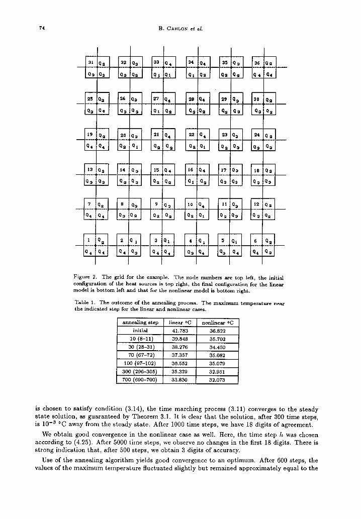
The final configurations, i.e., the distribution of the Q’s, after 700 steps of the annealing algorithm, are shown in Figure 2 as well. The distribution for the linear model is shown in the bottom left part of each square. That for the nonlinear model is in the bottom right part.

The maximum temperature decrease for each model is described in Table 1 below, where step 10 means the smallest maximum temperature between steps 8 and 11, etc. Clearly, the initial decreases are considerable while later decreases are less impressive.

The maximum temperature was found at node 22 in the linear case and node 17 in the nonlinear case, after 700 annealing steps. Initially the maximum was at node 33 in both cases.

We would like to point out that in this example, the number of possible permutations, i.e.,

possible configurations, is 36!

( 12!)2 8! 4! = 1.67 + 10’“.

This is the number of steps that a fully deterministic descent algorithm would have to perform. (If a step takes 1 second, it would take 53 billion years to complete the computation.)

During the runs, the value of the constant c* in (5.1) was reduced, at the annealing steps, in accordance with the discussion above. At the beginning it was halved every 30 annealing steps, and later every 70 steps. It would be of interest to perform more extensive computation to experiment with various ways of choosing the c*‘s. As was mentioned before, there seems to be no theoretical way to estimate them.

Physically, we observe that the lower power devices are being moved toward the upper part of the board where it is insulated, and the higher power devices to the lower part, where there is cooling by interaction with the wall in addition to the air stream. This explains the downward

drift of the location of the maximum temperature. We conclude that the annealing process converges in both cases and gives a configuration with

significantly lower maximum temperature. We see that for the linear model, when the time step

74 B. CAHLON et al.

_

Figure 2. The grid for the example. The node numbers are top left, the initial configuration of the heat sources is top right, the final configuration for the linear model is bottom left and that for the nonlinear model is bottom right.

Table 1. The outcome of the annealing process. The maximum temperature near the indicated step for the linear and nonlinear cases.

annealing step I linear OC I nonlinear OC

initial 41.783 36.822

10 (8-11) 39.848 35.702

30 (28-31) 36.276 34.450

70 (67-72) 37.357 35.082

100 (97-102) 36.552 35.079

300 (296-305) 35.329 32.951

1 700 (690-700) 1 33.830 32.073

is chosen to satisfy condition (3.14), the time marching process (3.11) converges to the steady state solution, as guaranteed by Theorem 3.1. It is clear that the solution, after 300 time steps, is 10S3 OC away from the steady state. After 1000 time steps, we have 18 digits of agreement.

We obtain good convergence in the nonlinear case as well. Here, the time step h was chosen according to (4.25). After 5000 time steps, we observe no changes in the first 18 digits. There is strong indication that, after 500 steps, we obtain 3 digits of accuracy.

Use of the annealing algorithm yields good convergence to an optimum. After 600 steps, the values of the maximum temperature fluctuated slightly but remained approximately equal to the

A model for the convective cooling 75

values in Table 1. (This lead us to stop the process after 700 steps.) In contrast, relatively large fluctuations were observed during the first 50 steps.

These numerical results are consistent with our theoretical results and suggest using both models in conjunction with the annealing algorithm to obtain optimal configurations of heat sources on a grid.

The examples were run on Oakland University’s Honeywell DP58 using the Multics operating system. All computation was done in double precision. We used the uniform (0,l) random number generator, which is built into the Multics system. The uniformly distributed number sequence was generated by the Tausworth method. To use it, one has to input an integer seed initially, which is updated thereafter.

1.

2. 3.

4.

5. 6.

7.

a.

9. 10. 11. 12. 13.

REFERENCES

D. Dancer and M. Pecht, Component-placement optimization for convectively cooled electronics, IEEE Trans. on Reliability 38, 199-205 (1989). D. Steinberg, Cooling Techniques for Electronic Equipment, Wiley, New York, (1982). R. Hmmemann, Electronic system thermal design for reliability, IEEE Tuna. on Reliability 26, 306-310 (1977). M. Osterman and M. Pecht, Component placement for reliability on conductively cooled printed wiring boards, ASME J. Electronic Packaging III, 149155 (1989). I. Gertsbakh, Optimal allocation of heat sources on a planar printed circuit board, Proc. ZMACS (1988). N. Metropolis, A.W. Rosenbluth, M N. Rosenbluth and A.M. Teller, Equations of state calculation by fast computing machines, J. Chem. Phys. 21, 1087-1092 (1953). S. Kirkpatrick, C. D. Gelatt, Jr. and M. P. Vecchi, Optimization by simulated meaiing, Research report RC 9355, IBM, Yorktown Heights, NY (1982). V. Cerny, A thermodynamic approach to the traveling salesman problem: An efficient simulation algorithm, J. Optim. Th. Appl. 45, 41-51 (1989). M. Lundy and A. Mees, Convergence of an annealing algorithm, Math. Frog. 34, 111-124 (1986). J. M. Ortega, Numerical Analysis, Academic Press, New York, (1972). Ft. A. Horn and C. R. Johnson, Matrix Analysis, Cambridge Univ. Press, Cambridge, (1988). J. Dieudomk, Foundations of Modern Analysis, Academic Press, New York, (1960). G.R. Beiitskii and Y.I. Lyubich, Matrix Norms and Their Applications, 0T36, Birkh&tser, Base& (1988).