A Mining Order-Preserving SubMatrices ... - HKUST CSE Dept.
44
A Mining Order-Preserving SubMatrices from Probabilistic Matrices QIONG FANG, Hong Kong University of Science and Technology WILFRED NG, Hong Kong University of Science and Technology JIANLIN FENG, Sun Yat-Sen University YULIANG LI, Hong Kong University of Science and Technology The Order-Preserving SubMatrices (OPSMs) capture consensus trends over columns shared by rows in a data matrix. Mining OPSM patterns discovers important and interesting local correlations in many real ap- plications, such as those involving biological data or sensor data. The prevalence of uncertain data in various applications, however, poses new challenges for OPSM mining, since data uncertainty must be incorporated into OPSM modeling and the algorithmic aspects. In this paper, we define new probabilistic matrix representations to model uncertain data with continuous distributions. A novel Probabilistic Order-Preserving SubMatrix (POPSM) model is formalized in order to capture similar local correlations in probabilistic matrices. The POPSM model adopts a new probabilistic support measure that evaluates the extent to which a row belongs to a POPSM pattern. Due to the intrinsic high computational complexity of the POPSM mining problem, we utilize the anti-monotonic property of the probabilistic support measure and propose an efficient Apriori-based mining framework called PROBAPRI to mine POPSM patterns. The framework consists of two mining methods, UNIAPRI and NORMAPRI, which are developed for mining POPSM patterns respectively from two representative types of probabilistic matrices, the UniDist matrix (assuming uniform data distributions) and the NormDist matrix (assuming normal data distributions). We show that the NORMAPRI method is practical enough for mining POPSM patterns from probabilistic matrices that model more general data distributions. We demonstrate the superiority of our approach by two applications. First, we use two biological datasets to illustrate that the POPSM model better captures the characteristics of the expression levels of biologically correlated genes, and greatly promotes the discovery of patterns with high biological significance. Our result is significantly better than the counterpart OPSMRM (OPSM with Repeated Measurement) model which adopts a set-valued matrix representation to capture data uncertainty. Second, we run the experiments on an RFID trace dataset and show that our POPSM model is effective and efficient in capturing the common visiting subroutes among users. Categories and Subject Descriptors: H.2.8 [Database Management]: Database Applications General Terms: Algorithms Additional Key Words and Phrases: order-preserving submatrices, probabilistic matrices, probabilistic sup- port, OPSM mining ACM Reference Format: Qiong Fang, Wilfred Ng, Jianlin Feng, and Yuliang Li, 2014. Mining Order-Preserving SubMatrices from Probabilistic Matrices. ACM Trans. Datab. Syst. 39, 1, Article A (January 2014), 44 pages. DOI:http://dx.doi.org/10.1145/0000000.0000000 This work is partially supported by Hong Kong RGC grants under project number GRF 617610 and T12- 403/11-2 and China NSF Grant 60970043. Author’s addresses: Q. Fang and W. Ng, Computer Science and Engineering Department, Hong Kong Univer- sity of Science and Technology; J. Feng, School of Software, Sun Yat-Sen University; Y. Li, (Current address) Computer Science and Engineering Department, University of California, San Diego. Permission to make digital or hard copies of part or all of this work for personal or classroom use is granted without fee provided that copies are not made or distributed for profit or commercial advantage and that copies show this notice on the first page or initial screen of a display along with the full citation. Copyrights for components of this work owned by others than ACM must be honored. Abstracting with credit is per- mitted. To copy otherwise, to republish, to post on servers, to redistribute to lists, or to use any component of this work in other works requires prior specific permission and/or a fee. Permissions may be requested from Publications Dept., ACM, Inc., 2 Penn Plaza, Suite 701, New York, NY 10121-0701 USA, fax +1 (212) 869-0481, or [email protected]. c 2014 ACM 0362-5915/2014/01-ARTA $15.00 DOI:http://dx.doi.org/10.1145/0000000.0000000 ACM Transactions on Database Systems, Vol. 39, No. 1, Article A, Publication date: January 2014.
-
Upload
khangminh22 -
Category
Documents
-
view
1 -
download
0
Transcript of A Mining Order-Preserving SubMatrices ... - HKUST CSE Dept.

A
Mining Order-Preserving SubMatrices from Probabilistic Matrices
QIONG FANG, Hong Kong University of Science and TechnologyWILFRED NG, Hong Kong University of Science and TechnologyJIANLIN FENG, Sun Yat-Sen UniversityYULIANG LI, Hong Kong University of Science and Technology
The Order-Preserving SubMatrices (OPSMs) capture consensus trends over columns shared by rows in adata matrix. Mining OPSM patterns discovers important and interesting local correlations in many real ap-plications, such as those involving biological data or sensor data. The prevalence of uncertain data in variousapplications, however, poses new challenges for OPSM mining, since data uncertainty must be incorporatedinto OPSM modeling and the algorithmic aspects.
In this paper, we define new probabilistic matrix representations to model uncertain data with continuousdistributions. A novel Probabilistic Order-Preserving SubMatrix (POPSM) model is formalized in order tocapture similar local correlations in probabilistic matrices. The POPSM model adopts a new probabilisticsupport measure that evaluates the extent to which a row belongs to a POPSM pattern. Due to the intrinsichigh computational complexity of the POPSM mining problem, we utilize the anti-monotonic property of theprobabilistic support measure and propose an efficient Apriori-based mining framework called PROBAPRI tomine POPSM patterns. The framework consists of two mining methods, UNIAPRI and NORMAPRI, which aredeveloped for mining POPSM patterns respectively from two representative types of probabilistic matrices,the UniDist matrix (assuming uniform data distributions) and the NormDist matrix (assuming normal datadistributions). We show that the NORMAPRI method is practical enough for mining POPSM patterns fromprobabilistic matrices that model more general data distributions.
We demonstrate the superiority of our approach by two applications. First, we use two biological datasetsto illustrate that the POPSM model better captures the characteristics of the expression levels of biologicallycorrelated genes, and greatly promotes the discovery of patterns with high biological significance. Our resultis significantly better than the counterpart OPSMRM (OPSM with Repeated Measurement) model whichadopts a set-valued matrix representation to capture data uncertainty. Second, we run the experiments onan RFID trace dataset and show that our POPSM model is effective and efficient in capturing the commonvisiting subroutes among users.
Categories and Subject Descriptors: H.2.8 [Database Management]: Database Applications
General Terms: Algorithms
Additional Key Words and Phrases: order-preserving submatrices, probabilistic matrices, probabilistic sup-port, OPSM mining
ACM Reference Format:Qiong Fang, Wilfred Ng, Jianlin Feng, and Yuliang Li, 2014. Mining Order-Preserving SubMatrices fromProbabilistic Matrices. ACM Trans. Datab. Syst. 39, 1, Article A (January 2014), 44 pages.DOI:http://dx.doi.org/10.1145/0000000.0000000
This work is partially supported by Hong Kong RGC grants under project number GRF 617610 and T12-403/11-2 and China NSF Grant 60970043.Author’s addresses: Q. Fang and W. Ng, Computer Science and Engineering Department, Hong Kong Univer-sity of Science and Technology; J. Feng, School of Software, Sun Yat-Sen University; Y. Li, (Current address)Computer Science and Engineering Department, University of California, San Diego.Permission to make digital or hard copies of part or all of this work for personal or classroom use is grantedwithout fee provided that copies are not made or distributed for profit or commercial advantage and thatcopies show this notice on the first page or initial screen of a display along with the full citation. Copyrightsfor components of this work owned by others than ACM must be honored. Abstracting with credit is per-mitted. To copy otherwise, to republish, to post on servers, to redistribute to lists, or to use any componentof this work in other works requires prior specific permission and/or a fee. Permissions may be requestedfrom Publications Dept., ACM, Inc., 2 Penn Plaza, Suite 701, New York, NY 10121-0701 USA, fax +1 (212)869-0481, or [email protected]© 2014 ACM 0362-5915/2014/01-ARTA $15.00DOI:http://dx.doi.org/10.1145/0000000.0000000
ACM Transactions on Database Systems, Vol. 39, No. 1, Article A, Publication date: January 2014.
A:2 Q. Fang et al.
PPPPPPGT
t1 t2 t3 t4
g1 10 8 6 15g2 8 7 4 9g3 2 12 9 14g4 6 10 12 7 5
10
15
20
t1 t2 t3 t4
Ent
ry v
alue
Column
g1g2g3g4
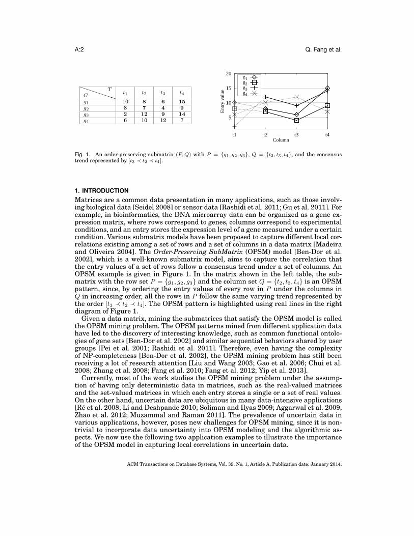
Fig. 1. An order-preserving submatrix (P,Q) with P = {g1, g2, g3}, Q = {t2, t3, t4}, and the consensustrend represented by [t3 ≺ t2 ≺ t4].
1. INTRODUCTIONMatrices are a common data presentation in many applications, such as those involv-ing biological data [Seidel 2008] or sensor data [Rashidi et al. 2011; Gu et al. 2011]. Forexample, in bioinformatics, the DNA microarray data can be organized as a gene ex-pression matrix, where rows correspond to genes, columns correspond to experimentalconditions, and an entry stores the expression level of a gene measured under a certaincondition. Various submatrix models have been proposed to capture different local cor-relations existing among a set of rows and a set of columns in a data matrix [Madeiraand Oliveira 2004]. The Order-Preserving SubMatrix (OPSM) model [Ben-Dor et al.2002], which is a well-known submatrix model, aims to capture the correlation thatthe entry values of a set of rows follow a consensus trend under a set of columns. AnOPSM example is given in Figure 1. In the matrix shown in the left table, the sub-matrix with the row set P = {g1, g2, g3} and the column set Q = {t2, t3, t4} is an OPSMpattern, since, by ordering the entry values of every row in P under the columns inQ in increasing order, all the rows in P follow the same varying trend represented bythe order [t3 ≺ t2 ≺ t4]. The OPSM pattern is highlighted using real lines in the rightdiagram of Figure 1.
Given a data matrix, mining the submatrices that satisfy the OPSM model is calledthe OPSM mining problem. The OPSM patterns mined from different application datahave led to the discovery of interesting knowledge, such as common functional ontolo-gies of gene sets [Ben-Dor et al. 2002] and similar sequential behaviors shared by usergroups [Pei et al. 2001; Rashidi et al. 2011]. Therefore, even having the complexityof NP-completeness [Ben-Dor et al. 2002], the OPSM mining problem has still beenreceiving a lot of research attention [Liu and Wang 2003; Gao et al. 2006; Chui et al.2008; Zhang et al. 2008; Fang et al. 2010; Fang et al. 2012; Yip et al. 2013].
Currently, most of the work studies the OPSM mining problem under the assump-tion of having only deterministic data in matrices, such as the real-valued matricesand the set-valued matrices in which each entry stores a single or a set of real values.On the other hand, uncertain data are ubiquitous in many data-intensive applications[Re et al. 2008; Li and Deshpande 2010; Soliman and Ilyas 2009; Aggarwal et al. 2009;Zhao et al. 2012; Muzammal and Raman 2011]. The prevalence of uncertain data invarious applications, however, poses new challenges for OPSM mining, since it is non-trivial to incorporate data uncertainty into OPSM modeling and the algorithmic as-pects. We now use the following two application examples to illustrate the importanceof the OPSM model in capturing local correlations in uncertain data.
ACM Transactions on Database Systems, Vol. 39, No. 1, Article A, Publication date: January 2014.

Mining Order-Preserving SubMatrices from Probabilistic Matrices A:3
Table I. A UniDist Matrix MU (G,T ) with G = {g1, g2, g3}and T = {t1, t2, t3, t4}PPPPPPG
Tt1 t2 t3 t4
g1 [7, 8] [6, 7] [2, 4] [10, 12]
g2 [4, 8] [7, 8] [3, 5] [14, 15]
g3 [4, 8] [3, 5] [3, 7] [9, 11]
Example 1.1. In gene expression analysis, the expression levels of genes under differ-ent experimental conditions are monitored. Due to inevitable noise contamination, theexperiment concerning a gene under a certain condition is usually repeated multipletimes, and the noisy replicates are assumed to follow a Gaussian (or normal) distribu-tion according to the studies in [Hughes et al. 2000; Lee et al. 2000]. Thus, to betterdescribe the characteristics of such noisy gene expression data, each entry in the geneexpression matrix, which corresponds to the expression level of a gene under a certaincondition, should be associated with a normal distribution. Although the OPSM modelis known to be effective for discovering biological correlations in real-valued gene ex-pression matrices [Ben-Dor et al. 2002], it has to be adapted for the gene expressionmatrix having normally distributed probabilistic data.
Example 1.2. In order to track visitors’ routes within a building, visitors are givenRFID tags to wear and they are detected by RFID readers (or antennas) [Re et al. 2008;Welbourne et al. 2008]. At an RFID detection site, a visitor may be continuously de-tected, which implies the probability of his/her stay at a particular location. Such RFIDdata can be organized as a probabilistic matrix where rows are visitors, columns areRFID detection sites, and each entry stores a time range indicating the stay of a visi-tor at a certain location. We are then able to find groups of visitors who likely share acommon visiting subroute, which can be represented by a probabilistic OPSM model.
To better model the data uncertainty as discussed in the above examples, we proposethe probabilistic matrices, where each entry is associated with a continuous probabilis-tic distribution. Two commonly used distributions are the uniform and normal distri-butions. When the uniform distribution is assumed, we call such a probabilistic matrixa UniDist matrix. Table I shows an example of a UniDist matrix with 3 rows and 4columns, denoted by MU (G,T ). The entry MU (g2, t3) stores a range [3, 5], which meansthat the corresponding entry value is uniformly distributed in the range between 3and 5.
In scientific studies, the normal distribution is fundamental to modeling empiricaldata distributions. For example, it is recognized that the normal distribution is de-sirable for modeling the noisy gene expression data generated from the microarrayexperiments [Hughes et al. 2000; Lee et al. 2000; Nguyen et al. 2010]. When the nor-mal distribution is considered, we call such a probabilistic matrix a NormDist matrixand denote it by MN (G,T ). An entry MN (gi, tj) in a NormDist matrix is representedby a pair (µij , σij), where µij and σij are respectively the mean and standard deviation.
In this paper, we focus on tackling the OPSM mining problem based on two typesof probabilistic matrices, the UniDist matrix and the NormDist matrix. However, weemphasize that the OPSM model defined based on the NormDist matrix and the corre-sponding mining method are flexible, in the sense that they can be adapted to dealingwith probabilistic matrices having more general continuous distributions. This benefitwill be further elaborated when the NormDist matrix is discussed.
Referring again to Figure 1, the submatrix (P,Q) is called an OPSM, if, for every rowin P , its entry values under columns in Q induce an identical order of Q. The induced
ACM Transactions on Database Systems, Vol. 39, No. 1, Article A, Publication date: January 2014.

A:4 Q. Fang et al.
(a) g1 under Q with τQ = [t3 ≺ t1 ≺ t4] (b) g2 under Q with τQ = [t3 ≺ t1 ≺ t4] andτ ′Q = [t1 ≺ t3 ≺ t4]
Fig. 2. Illustration of the order-preserving relationship in the UniDist matrix (g1 and g2 under Q ={t1, t3, t4} as shown in Table I). Given a range [l, u], the probability density within the range is computed by1
u−l.
order of a row g under Q is acquired by sorting the numerical entry values of g un-der Q in increasing order, and then replacing the values by the corresponding columnlabels. However, the concept of induced order of the OPSM model is not applicable toprobabilistic matrices.
Let us analyze the problem by referring to the UniDist matrix shown in Table I as anexample. If the range entries of row g1 under the columns Q = {t1, t3, t4} are arrangedalong the axis, we find that the values covered by the range MU (g1, t3) are smallerthan the values covered by the range MU (g1, t1), and in addition, the values coveredby both MU (g1, t3) and MU (g1, t1) are smaller than the values covered by the rangeMU (g1, t4), as illustrated in Figure 2(a). If the induced order of a row is determinedby the relationship among values in the ranges, we can say that the induced order ofrow g1 under Q is τQ = [t3 ≺ t1 ≺ t4], or in other words, row g1 supports the orderτQ. However, if we arrange the entries of row g2 under Q along the axis in a similarway, the entries MU (g2, t3) and MU (g2, t1) overlap on a subrange [4, 5], as illustrated inFigure 2(b). Thus, g2 is found to support both τQ and another possible order τ ′Q = [t1 ≺t3 ≺ t4]. A similar problem also exists in the NormDist matrix. The fact that a rowmay support more than one order in the probabilistic matrices makes it necessary toevaluate the extent to which a row supports an order. Intuitively, in the above example,g1 should be regarded as better supporting the order τQ than g2 does. Motivated by thisobservation, we define a new measure, called probabilistic support, to evaluate theextent to which a row supports an order, or in other words, it is the probability that arow is likely to induce an order. Based on the probabilistic support, a new OPSM modelcalled Probabilistic OPSM (POPSM) is defined.
Mining OPSM patterns from a real-valued matrix is an intrinsically difficult prob-lem, which is proved to be NP-complete [Ben-Dor et al. 2002]. When mining POPSMpatterns from the probabilistic matrices, we utilize the following strategies to designan efficient mining method. First, we prove the anti-monotonic property of the newprobabilistic support measure, and make use of it to control the number of candidatepatterns. Then, by combining a prefix-tree structure and the dynamic programmingtechniques, we are able to efficiently verify the candidate patterns and exhaustivelymine all valid POPSM patterns from the UniDist matrix and the NormDist matrix.
In summary, we tackle a new problem of mining probabilistic OPSM patterns. Themain contributions arising from this study are twofold.
ACM Transactions on Database Systems, Vol. 39, No. 1, Article A, Publication date: January 2014.

Mining Order-Preserving SubMatrices from Probabilistic Matrices A:5
— In the modeling aspect, we propose new probabilistic matrix representations to in-corporate the data uncertainty commonly existing in many applications. Based ontwo types of probabilistic matrices, namely the UniDist matrix and the NormDistmatrix, we define a new probabilistic OPSM model by adopting the probabilistic sup-port measure that evaluates the extent to which a row is likely to induce an order.We compare our model with the counterpart OPSM with Repeated Measurements(OPSMRM) model [Chui et al. 2008; Yip et al. 2013], which is defined based on theset-valued matrices. We demonstrate the superiority of the POPSM model by runningexperiments on two real biological datasets and one RFID dataset.Specifically, in the experiments using biological datasets, based on both the UniDistand NormDist matrices, the fraction of POPSM patterns that reach the highest sig-nificance level is larger than the fraction of the OPSMRM patterns that reach thesame level, while the fraction of the POPSM patterns that fall in the lowest signifi-cance level is less than that of the OPSMRM patterns at the same level. Using theRFID trace data, we show that the common subroutes of a set of users can be accu-rately discovered with the adoption of the POPSM model.
— In the algorithmic aspect, we propose an efficient Apriori-based POPSM miningframework called PROBAPRI. There are two versions of PROBAPRI, denoted byUNIAPRI and NORMAPRI, which, respectively, mine POPSM patterns from the Uni-Dist and NormDist matrices. PROBAPRI employs a CandTree structure to organizethe POPSM patterns. Two dynamic programming (DP) techniques are developed forcomputing the probabilistic support. By interweaving the traversal of CandTree andthe computation of the DP functions, the POPSM patterns can be efficiently veri-fied during the mining process. NORMAPRI adopts the spline technique [Heath 2002]to approximate the normal distributions with simpler low-degree polynomials. Theapproximation step is general enough to deal with other continuous distributions.Thus, NORMAPRI is capable of mining POPSM patterns from more general proba-bilistic matrices.
The organization of the rest of this paper is as follows. We present the related workin Section 2. The notations and terminologies are introduced in Section 3. In Section 4,after introducing the probabilistic support measure, we define the Probabilistic OPSM(POPSM) model. The POPSM mining method PROAPRI is discussed in Section 5. Ex-periments on synthetic and real datasets are presented in Section 6. Finally, we con-clude the paper in Section 7.
2. RELATED WORKThe problem of mining submatrix patterns was first studied over forty years ago for an-alyzing voting data [Hartigan 1972], where the voting data are organized as a matrixwith voters as rows, candidates as columns and voting scores as entries. It is nearlyimpossible to find a group of voters who gave the same voting scores over all the can-didates or to find a group of candidates who received the same voting scores from allthe voters, especially when the number of voters and candidates is large. However, it isalso observed that a subset of voters are likely to have common preferences over a sub-set of candidates, and such local correlations can be captured by submatrix patterns.As matrices become a common data representation in many application domains, theproblem of mining submatrix patterns has been extensively studied for revealing var-ious local correlations, which is usually known as subspace clustering [Parsons et al.2004; Kriegel et al. 2009], co-clustering [Wang et al. 2011; Ding et al. 2006; Ji et al.2012], and biclustering [Cheng and Church 2000; Madeira and Oliveira 2004]. We nowgive more details of the work.
ACM Transactions on Database Systems, Vol. 39, No. 1, Article A, Publication date: January 2014.

A:6 Q. Fang et al.
2.1. Subspace Clustering, Co-Clustering, and BiclusteringStudies about subspace clustering are motivated by the observation that the datapoints which are irrelevant in high dimensional space may be well clustered or corre-lated in lower dimensional subspaces [Parsons et al. 2004; Kriegel et al. 2009]. Thesestudies aim to identify a subset of attributes or features that form a subspace, and findthe data points that form a cluster over the subspace. If high-dimensional data areorganized as a matrix, the subspace features together with the clustered data pointscorrespond to the submatrix patterns in the matrix. However, different from the order-preserving relationship required by the OPSM model, the criteria for subspace clus-tering are usually the Euclidean distance between data points [Agrawal et al. 1998;Aggarwal et al. 1999; Moise and Sander 2008], the linearity correlation among datapoints [Gunnemann et al. 2012], the density of clusters [Kailing et al. 2004], or thestatistical significance of clusters [Moise and Sander 2008].
Another stream of submatrix pattern mining work aims to partition a matrix intogrid-distributed disjoint submatrices such that the subset of rows and the subset ofcolumns in each individual submatrix are expected to be highly correlated with eachother. This category of problems is usually called co-clustering, and has mainly beenstudied in recommender systems and text mining [Daruru et al. 2009; Banerjee et al.2004; Dhillon et al. 2003; Pan et al. 2008; Long et al. 2005; Ji et al. 2012]. The grid dis-tribution structure of submatrix patterns required by the co-clustering methods avoidsthe explosion of the number of mined patterns, which however is rather restrictive. Inorder to achieve a grid structure that optimizes the overall pattern scores, the qualityof a part of submatrix patterns usually has to be sacrificed.
Cheng and Church [Cheng and Church 2000] first adopted the submatrix miningmethods to analyze the biological gene expression data and called the problem bi-clustering. Biclustering methods aim to formulate different submatrix models so as tocapture the biological correlations among a subset of genes and a subset of conditions.Madeira et al. [Madeira and Oliveira 2004] classified existing submatrix models intofour categories: submatrix with constant values [Busygin et al. 2002], submatrix withconstant rows or constant columns [Getz et al. 2000; Pandey et al. 2009; Gupta et al.2010], submatrix with coherent values [Cho et al. 2004; Pontes et al. 2010], and sub-matrix with coherent evolutions [Murali and Kasif 2003; Tanay et al. 2002; Gupta andAggarwal 2010; Li et al. 2009; Madeira et al. 2010]. The OPSM model belongs to thefourth category according to this classification.
2.2. Mining Order-Preserving SubmatricesThe Order-Preserving Submatrix (OPSM) model, proposed by Ben-Dor et al. [Ben-Doret al. 2002], aims to capture the fact that the entry values of a set of rows exhibit thesame trend under a set of columns. A comparative study conducted by Prelic et al.[Prelic et al. 2006] showed that, compared to five other coherent-value or coherent-evolution submatrix models [Cheng and Church 2000; Prelic et al. 2006; Tanay et al.2002; Murali and Kasif 2003; Ihmels et al. 2002], the OPSM model better capturesthe association of correlated genes and conditions and promotes the discovery of alarger fraction of biologically significant patterns. However, it is also recognized thatthe OPSM model may be too strict to be practical, since real gene expression dataare noisy and the identical trend is usually hard to preserve [Ben-Dor et al. 2002]. Toaddress this problem, various noise-tolerant OPSM models have been proposed in liter-ature, such as the Approximate Order-Preserving Cluster (AOPC) model [Zhang et al.2008], the Relaxed Order-Preserving SubMatrix (ROPSM) model [Fang et al. 2010],the Bucket Order-Preserving SubMatrix (BOPSM) model [Fang et al. 2012], the Gen-eralized BOPSM (GeBOPSM) model [Fang et al. 2012], and the error-tolerated OPSM
ACM Transactions on Database Systems, Vol. 39, No. 1, Article A, Publication date: January 2014.

Mining Order-Preserving SubMatrices from Probabilistic Matrices A:7
model [Cheung et al. 2007]. The AOPC model relaxes the condition that all the rowsin an OPSM should induce the same linear order of columns, and only requires a pre-specified fraction of rows to induce the same linear order. The ROPSM model furtherrelaxes the AOPC model, and allows all the rows in an ROPSM pattern to induce or-ders similar to the backbone order of the pattern. The BOPSM model tries to capturethe consensus staged trend of a set of rows over a set of columns, and requires ev-ery row in a BOPSM pattern to induce an identical bucket order (i.e., an order of sets).The GeBOPSM model is a generalization of AOPC, ROPSM, and BOPSM. It allows therows in a GeBOPSM pattern to induce bucket orders which are similar to the backboneorder of the GeBOPSM pattern. The error-tolerated OPSM model still requires all therows in a pattern to induce an identical order of a set of columns but allows the entryvalues of a row under two adjacent columns to violate the ordering relationship withina pre-specified error threshold. However, due to different scalings of expression valuesof different genes, it is difficult to set a proper absolute error threshold to guaranteethat all the rows in a pattern still follow a consensus varying trend.
While the OPSM model and several other noise-tolerant OPSM models are all de-fined based on real-valued data matrices, an alternative way to address the issue ofnoisy data is to keep a set of replicates for each entry in the matrix, and such datamatrices can be presented as set-valued matrices [Hughes et al. 2000; Nguyen et al.2010; Ideker et al. 2001]. In a set-valued matrix, it is actually assumed that the set ofreplicates in every entry are equally likely to be observed. If an entry stores a set of kreplicates, all of them have an equal probability of 1
k . Therefore, a set-valued matrixcan be regarded as a probabilistic matrix with discrete distribution. Based on the set-valued matrices, an OPSM with Repeated Measurement (OPSMRM) model [Chui et al.2008; Yip et al. 2013] was introduced, where a fractional support measure is adopted toevaluate the extent to which a row supports a linear order. However, when the numberof replicates is small, as the noisy and true replicates have equally large probabilities,the fractional support is easily affected by one or two noisy replicates. On the otherhand, when the number of replicates grows, the cost of computing the fractional sup-port increases sharply, which greatly degrades the performance of mining OPSMRMpatterns.
Continuous distributions such as normal distribution are known to be effective forsmoothing out the influence of noise in scientific experiments, and thus are commonlyadopted to infer the error model of scientific data. For example, the observational errorin gene expression analysis, which may be caused by instrumental limits or measure-ment errors, is assumed to follow a normal distribution [Hughes et al. 2000; Nguyenet al. 2010; Chia and Karuturi 2010]. Thus, a gene expression matrix can be presentedas a probabilistic matrix with normal distribution. Probabilistic matrices are also anatural representation of the data arising from many sensor applications such as RFIDtracking systems [Re et al. 2008]. For example, when a user is detected at a particularRFID detection site within a time range, such trace data can then be represented asa probabilistic matrix with uniform distribution. The POPSM model proposed in thispaper is defined based on such probabilistic matrices with continuous distributions.We summarize the characteristics of the OPSM model and its variants in Table II.
Ben-Dor et al. proved that mining OPSM patterns is an NP-complete problem [Ben-Dor et al. 2002]. Then, they proposed a model-based method which aims to mine thebest OPSM in terms of the statistical significance, since patterns with high statisti-cal significance are regarded more likely to be biologically significant. Their methodkeeps a limited number of partial models which are smaller OPSM patterns. Then,it expands the partial models into larger and thus more statistically significant pat-terns. Their method, however, is heuristic-based, and the significance of the minedOPSM patterns is very sensitive to the selection of the partial models. Trapp et al.
ACM Transactions on Database Systems, Vol. 39, No. 1, Article A, Publication date: January 2014.

A:8 Q. Fang et al.
Table II. A Summary of OPSM Related Models
Models Matrix Types Pattern Characteristics References
OPSMReal-valued matrices Strict order-preserving
[Ben-Dor et al. 2002]
Twig OPSM [Gao et al. 2006]
AOPC
Real-valued matrices Relaxed order-preserving
[Zhang et al. 2008]
ROPSM [Fang et al. 2010]
BOPSM, GeBOPSM [Fang et al. 2012]
Error-tolerated OPSM [Cheung et al. 2007]
OPSMRM Set-valued matrices Fractional support to order[Chui et al. 2008]
[Yip et al. 2013]
POPSMProbabilistic matrices
Probabilistic support to order This workwith continuous distributions
[Trapp and Prokopyev 2010] and Humrich et al. [Humrich et al. 2011] both made useof integer programming techniques and proposed similar methods for mining the max-imal OPSM pattern. While Ben-Dor et al., Trapp et al., and Humrich et al.’s work allaimed to mine a single optimal OPSM pattern, Liu et al. [Liu and Wang 2003] pro-posed a tree-based OPSM mining method, called OPC-Tree, to exhaustively mine allthe OPSM patterns that satisfy some size thresholds. However, when the number ofcolumns in the data matrix increases, the size of the tree grows extremely large, andthe performance of pattern mining is greatly degraded. Cheung et al. [Cheung et al.2007] adopted the sequential pattern mining method in [Agrawal and Srikant 1995;Srikant and Agrawal 1996], and developed an Apriori-based method to exhaustivelymine OPSM patterns that satisfy some size thresholds. A post-processing solution wasadditionally designed to combine mined OPSM patterns into error-tolerated OPSMpatterns [Cheung et al. 2007]. Gao et al. proposed a KiWi framework in [Gao et al.2006; Gao et al. 2012] to mine twig OPSM patterns, which contain a large number ofcolumns and very few rows. The framework expands a limited number of linear ordersof columns in a breadth-first manner, and applies very strong conditions for pruningthose linear orders that are less likely to grow into twig OPSM patterns. Their methodis shown to be efficient but valid twig OPSM patterns may also get pruned. Zhang etal. [Zhang et al. 2008] adopted a similar pattern merging strategy as in [Cheung et al.2007] to mine AOPC patterns. Taking a set of OPSM patterns as input, The AOPCmining method merges pairs of OPSM patterns into AOPC patterns in a greedy wayuntil no more AOPC patterns can be generated. Fang et al. [Fang et al. 2010] proposeda pattern growth method, which expands seed OPSM patterns into ROPSM patterns.Later, they developed an Apriori-based method for mining BOPSM patterns and uti-lized the anti-monotonic property of the BOPSM model to control candidate generation[Fang et al. 2012]. However, the BOPSM model is defined based on the real-valued ma-trices and the rows in the BOPSM patterns are assumed to induce consensus bucketorders. Thus, the proof of the anti-monotonic property of the BOPSM model is differentfrom that of the anti-monotonic property of the POPSM model. An efficient prefix-treestructure was designed to maintain the BOPSM patterns, which motivates us to em-ploy the CandTree to compactly organize the POPSM patterns in this work.
The OPSMRM mining method [Chui et al. 2008; Yip et al. 2013] also follows theApriori-based framework, and consists of the following two steps. First, an Apriori-based method is taken to exhaustively mine frequent orders of columns. An order isregarded frequent if the sum of fractional supports contributed by all the rows exceedsa certain threshold. In this step, the anti-monotonic property of the fractional support
ACM Transactions on Database Systems, Vol. 39, No. 1, Article A, Publication date: January 2014.
Mining Order-Preserving SubMatrices from Probabilistic Matrices A:9
measure is made use of. However, as the fractional support is defined based on the set-valued matrices, its computation method and the proof of the anti-monotonic propertyare different from our work that involves the notion of probabilistic support. Then, foreach frequent order, the set of rows whose fractional supports to it satisfy another in-clusion threshold are picked. The selected rows, together with the columns involved inthe order, form an OPSMRM pattern. The inclusion threshold plays the similar role asthe support threshold in our POPSM model. The OPSMRM mining process, however,has the following implications. In the first step, although the fractional support of ev-ery row with respect to an order is small, this order may still be regarded as frequentdue to a large enough sum of the fractional supports contributed by all the rows. Thenin the second step, a frequent order may fail to lead to a valid OPSMRM pattern if noneof the rows has a large enough fractional support that satisfies the inclusion threshold.Another possibility is that, very few rows have large enough fractional supports withrespect to the frequent order, and this order finally leads to a very small and hencestatistically insignificant patterns [Ben-Dor et al. 2002].
2.3. Sequential Pattern MiningIf a data matrix is transformed into a set of attribute (i.e., column label) sequences or-dered by their values in every row, the matrix can be viewed as a transaction databasewith a collection of sequences. Accordingly, the OPSM mining problem is converted to afrequent sequential pattern mining problem [Agrawal and Srikant 1995; Srikant andAgrawal 1996].
However, due to some unique properties of the OPSM mining problem, using fre-quent sequential pattern mining methods for mining OPSM patterns is not satisfac-tory from the efficiency view point. First, each attribute appears at most once in eachsequence. Second, as the data matrices in an OPSM mining application are usuallyvery dense, the transformed sequences are also dense, in the sense that every attributemay appear in most of the sequences. As a result, the searching space of the depth-firstsequential pattern mining methods would be extremely large, while few candidatescan be pruned in the first few rounds of the breadth-first pattern mining methods. Liuet al. [Liu and Wang 2003] took into account the characteristics of the OPSM miningproblem, and proposed an OPSM mining method called OPC-Tree, which improves thebasic techniques of a well-known efficient frequent sequential pattern mining methodcalled PrefixSpan [Pei et al. 2001; Pei et al. 2004]. The OPC-Tree was shown to outper-form PrefixSpan in mining OPSMs. Agrawal et al. proposed an Apriori-based sequen-tial mining method [Agrawal and Srikant 1995; Srikant and Agrawal 1996], basedon which the BOPSM mining method [Fang et al. 2012] and the OPSMRM miningmethod [Chui et al. 2008] were respectively developed. The PROBAPRI method pro-posed in this work also adopts the Apriori-based framework, but we apply it to dealingwith the probabilistic data with continuous distributions. Kum et al. [Kum et al. 2003]studied the problem of mining approximate frequent sequential patterns. They firstclustered input sequences into disjoint sets, and then looked for consensus patternswithin each cluster. However, unlike the support requirement for mining OPSM pat-terns, the consensus patterns were evaluated based on their global support, and thusa frequent consensus pattern is not necessarily supported by a large enough numberof sequences.
Aggarwal et al. [Aggarwal et al. 2009], Muzammal et al. [Muzammal and Raman2011] and Zhao et al. [Zhao et al. 2012] studied the problem of mining frequent pat-terns or frequent sequential patterns in the context of uncertain data. However, theuncertain data are modeled as discrete values rather than continuous distributions.
ACM Transactions on Database Systems, Vol. 39, No. 1, Article A, Publication date: January 2014.

A:10 Q. Fang et al.
2.4. Modeling Probabilistic Data with Continuous DistributionsThe uncertain data in [Li and Deshpande 2010; Soliman and Ilyas 2009] are mod-eled using continuous distributions. But their work are related to the problem of top-kquery processing and ranking in uncertain databases. We are essentially studying thesubmatrix pattern mining problem. In Soliman et al.’s work, a positional probabilityis needed to be computed, and the formulation of the probability is similar to thatof our probabilistic support. However, they only considered the uniform distribution.The Monte-Carlo integration method proposed for computing the positional probabilityonly returns an approximate answer. In Li et al.’s work, the spline technique was alsoadopted to approximate complex continuous distributions with piecewise polynomials.However, the techniques they proposed to compute a parameterized ranking functionis totally different from the techniques we proposed for mining POPSM patterns.
Li et al. also discussed two other approximation techniques for continuous distri-butions, the Monte Carlo method and the discretization method. The Monte Carlomethod approximates a continuous distribution by a set of independent random sam-ples drawn from the distribution, which converts a probabilistic matrix to a set-valuedmatrix. This approximation is not applicable for mining POPSM patterns. The dis-cretization method approximates a continuous distribution by piecewise histograms,which can be perceived as a specialization of the spline approximation.
3. PRELIMINARIESIn this section, we introduce some notations and terminologies that are used through-out the paper.
3.1. UniDist Matrix and RangeWe denote an m-by-n UniDist matrix by MU (G,T ), where G is a set of m rows andT is a set of n columns (or items). The entry MU (gi, tj) under row gi and column tjis represented by a range Rij = [lij , uij ], where lij and uij are respectively the lowerand upper bounds of the range. We call the set of range entries of a row gi under thecolumns in T , i.e., {[li1, ui1], . . . , [lin, uin]}, the record of gi.
For each entry MU (gi, tj), its possible replicates are assumed to be uniformly dis-tributed within the range, and thus it can also be denoted by a random variable MU
ij
with its probability density function (PDF) given by
pUij(x) =
{1
uij−lij if x ∈ [lij , uij ]
0 otherwise.(1)
For example, the entryMU (g1, t3) in the UniDist matrix shown in Table I is [2, 4]. Thus,the corresponding random variable MU
13 has the probability density of 14−2 = 0.5 within
the range [2, 4] and 0 out of the range. When there is no ambiguity, we may use thenotations MU (gi, tj), Rij , [lij , uij ], and MU
ij interchangeably to represent an entry in agiven UniDist matrix.
In many real-life applications, the entry values in the data matrix are collected in-dependently. For example, when the DNA microarray technology is adopted for geneexpression analysis, the expression level of every gene under every condition is moni-tored and measured independently [Seidel 2008]. Therefore, the entries in the gener-ated gene expression matrix can be regarded as independent of each other. In the RFIDapplications, an RFID reader is supposed to detect different RFID tags separately andtwo RFID readers do not influence each other [Welbourne et al. 2008]. Thus, the in-dependence assumption also holds in the RFID data matrix. We now assume that therandom variables MU
ij , with 1 ≤ i ≤ m and 1 ≤ j ≤ n, be independent of each other.
ACM Transactions on Database Systems, Vol. 39, No. 1, Article A, Publication date: January 2014.

Mining Order-Preserving SubMatrices from Probabilistic Matrices A:11
Given a set of ranges {[l1, u1], . . . , [lk, uk]}, we can sort them in increasing or-der of their middle point values given by li+ui
2 , and get an ordered range set〈[li1 , ui1 ], . . . , [lik , uik ]〉, where 〈i1, . . . , ik〉 is a permutation of the values 1 to k. We saythat the range Ri = [li, ui] is smaller than (or larger than) the range Rj = [lj , uj ] if li+ui
2
is smaller than (or larger than) lj+uj2 . The difference between Ri and Rj , denoted by
D(Ri, Rj), is given by
D(Ri, Rj) = |li + ui
2− lj + uj
2|.
We say that two ranges Ri = [li, ui] and Rj = [lj , uj ] are disjoint if ui < lj or uj < li.Notably, the fact that Ri is smaller than (or larger than) Rj does not necessarily meanthat Ri and Rj are disjoint.
3.2. NormDist MatrixSimilarly to MU (G,T ), we denote a NormDist matrix by MN (G,T ). The entryMN (gi, tj) is represented by a normal distribution (µij , σij), where µij and σij are re-spectively the mean and the standard deviation. Similarly, we call the set of entriesof a row gi under the columns in T , i.e., {(µi1, σi1), . . . , (µin, σin)}, the record of gi. Inaddition, an entry MN (gi, tj) can be denoted by a random variable MN
ij with its PDFgiven by
pNij (x) =1√2πσ2
ij
e−
(x−µij)2
2σ2ij . (2)
Similarly to MUij , the random variables in a NormDist matrix, MN
ij with 1 ≤ i ≤ mand 1 ≤ j ≤ n, are also regarded as mutually independent. When there is no ambiguity,we use the notations MN (gi, tj), (µij , σij), and MN
ij interchangeably to represent anentry.
Given two random variables MN1 and MN
2 with the normal distributions (µ1, σ1) and(µ2, σ2), we say that MN
1 is smaller than (or larger than) MN2 if µ1 < µ2 (or µ1 > µ2).
The difference between MN1 and MN
2 , denoted by D(MN1 ,M
N2 ), is given by
D(MN1 ,M
N2 ) = |µ1 − µ2|.
3.3. Probabilistic MatricesWhen there is no ambiguity, we collectively call both the UniDist matrix and the Norm-Dist matrix as the probabilistic matrices and use M(G,T ) to denote such matrices. Theentry M(gi, tj) with gi ∈ G and tj ∈ T is also denoted by Mij .
3.4. OrderGiven a set of k items Q = {t1, . . . , tk}, a linear order (or simply an order) of Q isrepresented as τQ = [ti1 ≺ ti2 ≺ · · · ≺ tik ], and the ordering relation “ ≺ ” satisfies thecriteria of antisymmetry, transitivity, and linearity. Q is called the associated item setof τQ, and τQ is said to be a size-k order.
Given two orders τ1 and τ2 with their associated item sets Q1 and Q2, we say thatτ1 is a sub-order of τ2, if Q1 ⊆ Q2, and for all pairs of items ti, tj ∈ Q1, (ti ≺ tj) ∈ τ1implies (ti ≺ tj) ∈ τ2.
4. THE PROBABILISTIC OPSM MODELIn this section, we first introduce a new measure, called probabilistic support, to eval-uate the extent to which a row probably induces (or supports) an order. We then incor-
ACM Transactions on Database Systems, Vol. 39, No. 1, Article A, Publication date: January 2014.

A:12 Q. Fang et al.
Fig. 3. Relative positions between two ranges R1 and R2
porate this measure into a new OPSM model called Probabilistic OPSM (or POPSMfor short).
4.1. Probabilistic Support MeasureDefinition 4.1 (Probabilistic Support). Given a row gi and a set of columns Q in a
probabilistic matrix M , the probabilistic support of gi with respect to (w.r.t.) τQ = [t1 ≺· · · ≺ tr], denoted by PS(gi, τQ), is given by
PS(gi, τQ) = P (Mi1 < Mi2 < · · · < Mir),
where Mij is the random variable corresponding to the entry M(gi, tj) with 1 ≤ j ≤ r,and P (Mi1 < · · · < Mir) is the probability that the random event (Mi1 < · · · < Mir)occurs.
Based on the theory of order statistics [Ahsanullah et al. 2013], given a set of randomvariables M1,M2, . . . ,Mr with the corresponding PDFs as p1(x), p2(x), . . ., pr(x), theprobability of the random event (M1 < · · · < Mr) is given by
P (M1 < · · · < Mr) =
∫ +∞
−∞p1(x1)dx1
r∏i=2
[∫ +∞
xi−1
pi(xi)dxi
]. (3)
In a UniDist matrix, the PDF of a random variable is given in Formula (1), and allthe random variables are independent of each other as we have illustrated in Section3. By replacing the PDF pi(x) of Mi with I(x∈Ri)
ui−li , Formula (3) is transformed into thefollowing expression:
P (M1 < · · · < Mr) =
∫ +∞
−∞
I(x1 ∈ R1)
u1 − l1dx1
r∏i=2
[∫ +∞
xi−1
I(xi ∈ Ri)
ui − lidxi
],
=
∫ +∞−∞ I(x1 ∈ R1)dx1
∏ri=2
[∫ +∞xi−1
I(xi ∈ Ri)dxi
]∏r
i=1(ui − li), (4)
where Ri = [li, ui] is the range corresponding to Mi and I(·) is an indicator function.We now use two random variables M1 and M2 with uniform distribution to illustrate
how the probability of the random event (M1 < M2) varies with the relative positionof the two corresponding ranges. Suppose that the associated ranges of M1 and M2 arerespectively R1 = [l1, u1] and R2 = [l2, u2], and the range sizes (u1− l1) and (u2− l2) arefixed. There are altogether six possible relative positions between R1 and R2 as shownin Figure 3.
— Case (a): R1 is smaller than R2, and they are disjoint. In this case, the probability is1.0.
ACM Transactions on Database Systems, Vol. 39, No. 1, Article A, Publication date: January 2014.

Mining Order-Preserving SubMatrices from Probabilistic Matrices A:13
— Case (b): R1 is smaller than R2, but they overlap each other. According to Formula(4), the probability is given by
1− (u1 − l2)2
2(u1 − l1)(u2 − l2).
There are three sub-cases concerning the varying trend of the probability.• If (u1−l1) < (u2−l2), asD(R1, R2) decreases from (u2−l1)
2 to (u2−u1)2 , the probability
monotonically decreases from 1 to(1− u1−l1
2(u2−l2)
);
• if (u1− l1) > (u2− l2), as D(R1, R2) decreases from (u2−l1)2 to (l2−l1)
2 , the probabilitymonotonically decreases from 1 to
(1− u2−l2
2(u1−l1)
);
• if (u1 − l1) = (u2 − l2), as D(R1, R2) decreases from (u2−l1)2 to 0, the probability
monotonically decreases from 1 to 12 .
For all three sub-cases, the probability monotonically decreases as D(R1, R2) getssmaller.
— Case (c): R2 contains R1. In this case, the probability falls in the range[u1 − l1
2(u2 − l2), 1− u1 − l1
2(u2 − l2)
].
When D(R1, R2) equals to 0, the probability equals to 12 .
— Case (d): R1 contains R2. This case is symmetric with Case (c), and the probabilityfalls in the range [
u2 − l22(u1 − l1)
, 1− u2 − l22(u1 − l1)
].
When D(R1, R2) equals 0, the probability equals 12 .
— Case (e): R1 is larger than R2, and they overlap each other. In this case, the proba-bility is given by
(u2 − l1)2
2(u1 − l1)(u2 − l2).
Similarly to Case (b), there are also three sub-cases concerning the varying trend ofthe probability.• If (u1− l1) < (u2− l2), as D(R1, R2) increases from (l1−l2)
2 to (u1−l2)2 , the probability
monotonically decreases from u1−l12(u2−l2) to 0;
• if (u1− l1) > (u2− l2), as D(R1, R2) increases from (u1−u2)2 to (u1−l2)
2 , the probabilitymonotonically decreases from u2−l2
2(u1−l1) to 0;
• if (u1 − l1) = (u2 − l2), as D(R1, R2) increases from 0 to (u1−l2)2 , the probability
monotonically decreases from 12 to 0.
For all three sub-cases, the probability monotonically decreases as D(R1, R2) getslarger.
— Case (f): R1 is larger than R2 and they are disjoint. In this case, the probabilityequals 0.
Considering the probability P (M1 < M2), where M1 and M2 are random variablesthat follow normal distribution, we can observe the varying trends similar to that ofuniform distribution. In other words, when M1 is smaller than M2, the probability islarger than 0.5, and monotonically decreases from 1 to 0.5 as D(M1,M2) gets smaller.
ACM Transactions on Database Systems, Vol. 39, No. 1, Article A, Publication date: January 2014.

A:14 Q. Fang et al.
When M1 is larger than M2, the probability is smaller than 0.5 and monotonicallydecreases from 0.5 to 0 as D(M1,M2) gets larger. Strictly speaking, the domain ofa normal distribution is infinite, and thus the probability only infinitely approaches 1whenM1 is smaller thanM2 andD(M1,M2) gets extremely large. At the other extreme,the probability infinitely approaches 0 when M2 is smaller than M1 and D(M1,M2)gets extremely large.
From the above analysis, Formula (3) well reflects the positional relationship andthe difference between random variables. Thus, we adopt Formula (3) to formulate ourprobabilistic support measure.
The probabilistic support holds the anti-monotonic property, which is formally statedin Theorem 4.2.
THEOREM 4.2. [Anti-Monotonicity] Given a threshold α, if the probabilistic supportof a row g w.r.t. an order τQ is larger than or equal to α, the probabilistic support of gw.r.t. all the sub-orders of τQ is also larger than or equal to α.
Proof: Let g be a row and {t1, . . . , tk} be a set of k columns in a probabilistic matrix.Suppose the entries of g under {t1, . . . , tk} correspond to the random variables {M1, . . . ,Mk}. To establish the proof, we only need to show that
P (M1 < · · · < Mk) ≤ P (M1 < · · · < Mr−1 < Mr+1 < · · · < Mk),
with 1 ≤ r ≤ k, which is straightforward.Since the occurrence of the random event (M1 < · · · < Mk) implies the occurrence of
the event (M1 < · · · < Mr−1 < Mr+1 < · · · < Mk), the probability P (M1 < · · · < Mk) isthus no larger than the probability P (M1 < · · · < Mr−1 < Mr+1 < · · · < Mk). 2
4.2. The POPSM ModelUsing the probabilistic support measure, we now formalize the probabilistic OPSMmodel.
Definition 4.3 (Probabilistic OPSM (POPSM)). Given a probabilistic matrixM(G,T ) and a support threshold α, a submatrix (P,Q) with P ⊆ G and Q ⊆ T issaid to be a POPSM pattern, if there exists an order τQ such that, for all gi ∈ P , theprobabilistic support gi w.r.t. τQ is larger than or equal to α, that is,
∀gi ∈ P ,PS(gi, τQ) ≥ α.
We call the order τQ the backbone order of the POPSM (P,Q), and the rows in P thesupporting rows of τQ.
Since a POPSM pattern (P,Q) is associated with a backbone order τQ, we denotesuch a pattern by (P,Q : τQ). A POPSM pattern (P,Q : τQ) is said to be maximal, ifthere does not exist any other POPSM pattern (P ′, Q′ : τQ′) such that P ⊆ P ′, Q ⊆ Q′,and τQ is a sub-order of τQ′ .
Based on the anti-monotonic property of the probabilistic support, we are able tostraightforwardly deduce that the POPSM model also satisfies the anti-monotonicproperty. That means, given a POPSM pattern (P,Q : τQ), all the submatrices (P ′, Q′)of (P,Q) are also POPSM patterns with the backbone order τQ′ being a sub-order ofτQ. We will make use of the anti-monotonic property of the POPSM model to developan efficient POPSM mining algorithm in Section 5.
Now, we formally define the POPSM mining problem.
Definition 4.4 (The POPSM Mining Problem). Given a probabilistic matrixM(G,T ), a support threshold α, and two size thresholds rmin and cmin, we aim to
ACM Transactions on Database Systems, Vol. 39, No. 1, Article A, Publication date: January 2014.

Mining Order-Preserving SubMatrices from Probabilistic Matrices A:15
ALGORITHM 1: PROBAPRI
Input: Probabilistic matrix M(G,T ); support threshold α; size thresholds rmin and cmin
Variable: Ck - the set of size-k candidate orders; Fk - the set of size-k frequent ordersF1 ={size-1 frequent orders};for (k = 2;Fk−1 6= φ; k ++) doCk= GENCAND(Fk−1) ;COUNTSUP(M, Ck, α);Fk = {τ |τ ∈ Ck, supp(τ) ≥ rmin} ;if k ≥ cmin && Fk 6= φ then
Put POPSM patterns in output pool;end
endOutput maximal POPSM patterns;
exhaustively mine from M all the maximal POPSM patterns that contain at least rmin
rows and cmin columns.
As very small patterns possibly exist in the matrix randomly and they are likely toreveal trivial biological correlations [Ben-Dor et al. 2002; Liu and Wang 2003; Fanget al. 2010], we include two size thresholds rmin and cmin in Definition 4.4 to avoidmining too many small POPSM patterns.
5. MINING PROBABILISTIC OPSMIn this section, we exploit the anti-monotonic property of the POPSM model andadopt an Apriori-based framework to develop a new POPSM mining method calledPROBAPRI. There are two versions of PROBAPRI, UNIAPRI and NORMAPRI, respec-tively developed for mining POPSM patterns from the UniDist matrix and the Norm-Dist matrix. If not explicitly specified, the procedures presented are applicable to bothUNIAPRI and NORMAPRI.
5.1. PROBAPRI AlgorithmGiven a probabilistic matrix M(G,T ) and a support threshold α, a naıve way to minePOPSM patterns can be carried out as follows: for every set of columns Q with Q ⊆ Tand |Q| ≥ cmin, and every possible order τQ of Q, we simply check all the rows inG to examine if the probabilistic support of a row w.r.t. τQ is larger than or equalto α. Let P be the set of supporting rows of τQ. If |P | ≥ rmin, then (P,Q) is a validPOPSM pattern with τQ as the backbone order. However, such an exhaustive search isapparently infeasible, since the number of such orders is prohibitively large, especiallywhen the number of columns in T is large.
The anti-monotonic property of the POPSM model is important in developing a moreefficient approach for mining POPSM patterns. Intuitively, before searching the sup-porting rows of an order, we first check whether all its sub-orders are supported by atleast rmin rows. If not, we then confirm that the order does not give rise to any validPOPSM and, thus, can be discarded. This idea motivates us to develop an Apriori-based framework to mine POPSM patterns, as detailed in Algorithm 1.
In Algorithm 1, if a size-k order has at least rmin supporting rows, we call it a size-kfrequent order. Any size-k order can be a size-k candidate order. We denote by Ck andFk a set of size-k candidate orders and the set of all size-k frequent orders, respectively.First, the set of size-1 frequent orders, i.e., F1, is generated, which contains orders withevery single column in T . Then, the GENCAND procedure detailed in Section 5.2 is in-voked to generate Ck from Fk−1. The candidate generation algorithm GENCAND aimsto reduce the size of Ck as much as possible, but still guarantees that all the size-k
ACM Transactions on Database Systems, Vol. 39, No. 1, Article A, Publication date: January 2014.

A:16 Q. Fang et al.
F3: five size-3 frequent orders
τ1 [t1 ≺ t2 ≺ t3]
τ2 [t1 ≺ t2 ≺ t4]
τ3 [t1 ≺ t3 ≺ t4]
τ4 [t2 ≺ t3 ≺ t4]
τ5 [t2 ≺ t4 ≺ t3]
Fig. 4. A CandTree example
frequent orders are included in Ck. Next, the COUNTSUP procedure detailed in Section5.3 is invoked to verify the candidate orders in Ck. Specifically, the COUNTSUP proce-dure counts the number of supporting rows for each candidate order. Those candidateorders that are supported by at least rmin rows are called the size-k frequent ordersand form the set Fk. If k is larger than or equal to cmin and Fk is not empty, the POPSMpatterns (P,Q : τQ) are placed in an output pool, where τQ is a frequent order in Fk,and P is the set of supporting rows of τQ. Finally, we output those maximal POPSMpatterns as the result.
5.2. Candidate GenerationThe GENCAND procedure generates the set of size-k candidate orders Ck. This proce-dure applies to both the UniDist matrix and the NormDist matrix.
Since the candidate order set Ck must contain all the size-k frequent orders, wemay simply include in Ck all possible size-k orders. However, the size of Ck increasesexponentially when k gets larger. As all the candidate orders in Ck need to be furtherverified in COUNTSUP which is a time-consuming process, we expect to exclude from Ckas many as possible orders which cannot be frequent. The anti-monotonic property isutilized to achieve this goal. Based on the property, a size-k order cannot be a frequentorder if any of its size-(k − 1) sub-order is not frequent. Therefore, the search spacefor size-k candidate orders can be restricted to the size-k orders, of which all the size-(k − 1) sub-orders are in Fk−1. The GENCAND procedure is thus designed to generateCk based on Fk−1.
A prefix-sharing tree structure called CandTree is employed to organize frequent orcandidate orders, and the candidate generation process is implemented by updatingthe tree. Figure 4 presents a CandTree example, where five size-3 frequent orders arelisted in the left table, and the subtree inside the rectangle in the right diagram is thecorresponding CandTree. In the CandTree, all the orders are organized in the prefix-sharing manner, and a path leading from root to a leaf node exactly corresponds to anorder. For example, the rightmost path leading from root to nodes t2, t4, and finally t3corresponds to the order τ5 in the table. Each leaf node in the CandTree is associatedwith a bitmap, where the ith bit corresponds to the ith row in the input probabilisticmatrix. It is set to 1 if the probabilistic support of row gi to the corresponding order islarger than or equal to the threshold α; otherwise, it is set to 0. Note that the nonleafnodes in the CandTree of Fk−1 were once leaf nodes in the CandTree of Fr with r <(k − 1). Thus, every node in the CandTree except root is actually associated with abitmap.
ACM Transactions on Database Systems, Vol. 39, No. 1, Article A, Publication date: January 2014.

Mining Order-Preserving SubMatrices from Probabilistic Matrices A:17
ALGORITHM 2: GENCAND
Input: CandTree(Fk−1)Output: CandTree(Ck)Variable: τ [p] - the order corresponding to the path from root to pwhile there are unvisited nodes in CandTree(Fk−1) do
Depth-first traversal to node p with |τ [p]| = k − 2;for p’s child nodes t1 and t2 do
Insert t2 as a child of t1;end
endfor all newly inserted leaf nodes t do
if any size-(k − 1) sub-order of τ [t] /∈ Fk−1 thenUndo insertion of node t;
endendPrune the subtrees not containing any newly-inserted leaf node.
The GENCAND procedure takes the CandTree of Fk−1 as input and returns an up-dated CandTree, where each path leading from root to a leaf node exactly correspondsto a size-k candidate order. We call the updated tree the CandTree of Ck. GENCANDconsists of three steps, and the details are shown in Algorithm 2. First, given theCandTree of Fk−1, a depth-first traversal is carried out. When there are still unvisitednodes, the tree traversal continues until a non-leaf node p is reached such that thenumber of nodes along the path leading from root to p (with root excluded) is k − 2.For each pair of p’s child nodes t1 and t2, t2 is inserted as a child of t1. In this step,instead of inserting all the size-k orders, we only insert those orders, of which the twosize-(k − 1) sub-orders that share a size-(k − 2) prefix are frequent. The search spaceof size-k candidate orders is thus reduced. After finishing the tree traversal, for eachnewly inserted node t, the path leading from root to t forms a size-k order τ [t]. Then, apruning step is carried out to further examine whether all the size-(k−1) sub-orders ofτ [t] are in Fk−1. If not, τ [t] is surely not a frequent order, and can be excluded from Ckas well. Thus, the insertion of node t is revoked. Since the size-(k − 1) frequent ordersare stored in the CandTree of Fk−1, the pruning step can be efficiently accomplishedby scanning the CandTree. After pruning, the remaining size-k orders form the set ofsize-k candidate orders Ck. Finally, the tree is trimmed by deleting those subtrees thatdo not contain any newly inserted leaf node, since these subtrees do not lead to anyvalid size-k candidate orders. The updated tree is the CandTree of Ck.
We further illustrate GENCAND using the example in Figure 4. The CandTree ofF3 is traversed until node t2, which is marked with “∗”, is reached. For the two childnodes of t2 (i.e., t3 and t4), one is inserted as a child of the other. Then, the tree traversalcontinues until all the nodes are visited. Finally, only two new leaf nodes (i.e. t3 andt4) are inserted, which are highlighted in bold font. For the newly inserted node t4, thepath leading from root to it represents the order τ [t4] = [t1 ≺ t2 ≺ t3 ≺ t4]. Since allthe size-3 sub-orders of τ [t4], i.e., τ1, τ2, τ3 and τ4 in the table of F3, are frequent, τ [t4]is a size-4 candidate order. Similarly, the path leading from root to the other newlyinserted node t3 corresponds to another size-4 order τ [t3] = [t1 ≺ t2 ≺ t4 ≺ t3]. One ofthe size-3 sub-orders of τ [t3], i.e., [t1 ≺ t4 ≺ t3], is not in F3, which means that it is notfrequent. Thus, the order τ [t3] is surely not a frequent order and the insertion of nodet3 is revoked. Finally, we prune three subtrees with their root nodes marked with “#”,since none of these three subtrees contains any newly inserted leaf node and so theywould not lead to any size-4 candidate order. The updated tree is the CandTree of C4.
ACM Transactions on Database Systems, Vol. 39, No. 1, Article A, Publication date: January 2014.

A:18 Q. Fang et al.
Notably, GENCAND is said to be complete, in the sense that all size-k frequent ordersare included in Ck. We now justify its completeness.
Assume that Fk−1 contains all size-(k − 1) frequent orders. Let τ = [t1 ≺ · · · ≺ tk] bea size-k frequent order. According to the anti-monotonic property of the probabilisticsupport, all the supporting rows of τ should also be the supporting rows of the size-(k − 1) sub-orders of τ . In other words, if τ is a frequent order, all the size-(k − 1)sub-orders of τ must also be frequent and in Fk−1. Suppose there are τ1 = [t1 ≺ · · · ≺tk−2 ≺ tk−1] and τ2 = [t1 ≺ · · · ≺ tk−2 ≺ tk], which are two frequent size-(k − 1) sub-orders of τ . Since τ1 and τ2 only differ in the last item, the node that corresponds toitem tk−1 in τ1 and the node that corresponds to item tk in τ2 are two leaf nodes in theCandTree of Fk−1, and they share the same parent node tk−2. According to GENCAND,a new node tk is then inserted as a child node of tk−1, and the path leading from rootto the newly inserted tk corresponds to the order τ . As all the size-(k − 1) sub-ordersof τ are frequent and in Fk−1, the insertion of the new node tk does not get revoked inthe pruning step. Thus, the order τ is generated and added to Ck.
5.3. Support CountingAfter the set of size-k candidate orders Ck is generated, the COUNTSUP procedure isinvoked to verify whether the orders in Ck are frequent or not. Dynamic programming(DP) techniques are developed to compute the probabilistic support of a row w.r.t. acandidate order. If the probabilistic support of at least rmin rows w.r.t. a candidateorder is larger than or equal to the support threshold α, the candidate order is calledfrequent. The frequent candidate orders form the size-k frequent order set Fk.
We develop two DP techniques, respectively called static DP (SDP) and dynamicDP (DDP), for computing the probabilistic support of a row w.r.t. a candidate order.SDP disregards the size of the candidate order to which the probabilistic support iscomputed, and breaks down the computation into a fixed number of subproblems. Incontrast, for a candidate order with smaller size, DDP breaks down the computationof its probabilistic support into a fewer number of subproblems. Furthermore, whenthese two techniques are adopted to compute the probabilistic support w.r.t. the samecandidate order, the number of subproblems divided by DDP is no more than the num-ber of subproblems divided by SDP. Thus, compared to SDP, DDP saves computationalcost by solving fewer number of subproblems. However, DDP has to spend some extratime for dynamically forming the subproblems when running the process of dynamicprogramming. Our experiments in Section 6.4 show that both techniques exhibit theirefficiency under different scenarios. For the sake of clarity, when we employ SDP orDDP to compute the probabilistic support of a row w.r.t. a candidate order in a UniDistmatrix, we respectively call them the UNISDP and UNIDDP methods. When they areemployed to compute the probabilistic support in a NormDist matrix, we respectivelycall them the NORMSDP and NORMDDP methods. Table III summarizes the four DPmethods corresponding to different probabilistic matrices.
Table III. The DP methods corresponding to different types of probabilistic ma-triceshhhhhhhhhhhhhDP Technique
Matrix TypeUniDist Matrix NormDist Matrix
Static DP UNISDP NORMSDP
Dynamic DP UNIDDP NORMDDP
For either SDP or DDP, its recursive DP equations for the two types of matrices aresimilar, except that more complex preprocessing steps are needed when it is applied to
ACM Transactions on Database Systems, Vol. 39, No. 1, Article A, Publication date: January 2014.

Mining Order-Preserving SubMatrices from Probabilistic Matrices A:19
Fig. 5. The effective range [y2, x2] = [3, 15] of row g2 (in Table I) and its six subranges {s(1)2 , . . . , s(6)2 }
the NormDist matrix. For simplicity in presentation, the formulation of the DP equa-tions which is common for UniSDP and NormSDP (or respectively for UniDDP andNormDDP) is detailed when we introduce UniSDP (or respectively UniDDP). Whenintroducing NormSDP and NormDDP, we just focus on explaining the different pre-processing steps adopted by them. Then, we show that the COUNTSUP procedure com-bines any of the DP methods with the traversal of CandTree to compute the probabilis-tic support of a row w.r.t. all the candidate orders in Ck in an efficient way.
5.3.1. Static DP for UniDist matrix - UNISDP. We now detail the UNISDP method for com-puting the probabilistic support of a row w.r.t. an order in an m-by-n UniDist matrixMU (G,T ). Before applying the dynamic programming technique, there are two pre-processing steps to be carried out as follows:
(1) First, for the record of each row gi, i.e., {[li1, ui1], . . . , [lin, uin]}, we define xi =max{uij |1 ≤ j ≤ n} and yi = min{lij |1 ≤ j ≤ n}. The range [yi, xi] is called theeffective range of gi. Every range entry [lij , uij ] with 1 ≤ j ≤ n is fully covered bythe effective range, and the probability that any corresponding random variableMij is located outside the effective range is 0.
(2) Then, all lij ’s and uij ’s with 1 ≤ j ≤ n are sorted in non-decreasing order, and these2n values divide the range [yi, xi] into pi subranges s(j)i with 1 ≤ j ≤ pi. The numberof subranges pi is at most 2n− 1. We sort the pi subranges in nondecreasing orderof their middle point values, and get an ordered subrange set Si = 〈s(1)i , . . . , s
(pi)i 〉
corresponding to row gi. Note that for any two adjacent subranges in Si, thereexists at least one random variable in {Mi1, . . . ,Min} such that, its probabilitydensities in these two subranges are different.
Figure 5 shows the effective range of row g2 in Table I which is [3, 15]. The effectiverange is divided into six subranges that are sorted and indicated as 〈s(1)2 , . . ., s(6)2 〉.
Given a row gi with its ordered subrange set Si = 〈s(1)i , . . . , s(pi)i 〉, and a size-k order
τQ = [tj1 ≺ tj2 ≺ · · · ≺ tjk ], the probabilistic support of gi w.r.t. τQ, i.e., PS(gi, τQ) =P (Mij1 < · · · < Mijk), is computed as follows.
We first create a table ZU (R,C) with k rows and pi columns for dynamic program-ming. The xth row rx corresponds to the size-x prefix sub-order of τQ, i.e., [tj1 ≺ · · · ≺tjx ], and the yth column cy corresponds to the first y subranges in Si, i.e., 〈s(1)i , . . . , s
(y)i 〉.
The entry ZU (rx, cy) is the probability of the random event (Mij1 < · · · < Mijx) withMij1 , . . . ,Mijx located in the first y subranges. Thus, the entry ZU (rk, cpi) is the proba-bility of the event (Mij1 < · · · < Mijk) with Mij1 , . . . ,Mijk in all the pi subranges, whichactually is PS(gi, τQ). Further, the entry ZU (rx, cy) equals the sum of the followingthree parts:
ACM Transactions on Database Systems, Vol. 39, No. 1, Article A, Publication date: January 2014.

A:20 Q. Fang et al.
(1) the probability of (Mij1 < · · · < Mijx) with Mij1 , . . ., Mijx in the first (y − 1) sub-ranges; and
(2) the probability of (Mij1 < · · · < Mijx) with Mij1 , . . ., Mijx in the yth subrange; and(3) the probability of (Mij1 < · · · < Mijz ) with 1 ≤ z < x and Mij1 , . . ., Mijz in the
first (y − 1) subranges, multiplied by the probability of (Mij(z+1)< · · · < Mijx) with
Mij(z+1), . . ., Mijx in the yth subrange s(y)i .
The dynamic programming equation can then be written as:
ZU (rx, cy) = ZU (rx, cy−1) + P (Mij1 < · · · < Mijx |s(y)i )+
x−1∑z=1
ZU (rz, cy−1)P (Mij(z+1)< · · · < Mijx |s
(y)i ), (5)
where P (Mij1 < · · · < Mijx |s(y)i ) is the probability of the event (Mij1 < · · · < Mijx) with
Mij1 , . . . ,Mijx in the subrange s(y)i . As Mij1 , . . ., Mijx all follow uniform distributionswith the PDFs pij1 , . . ., pijx , P (Mij1 < · · · < Mijx |s
(y)i ) is then computed as
P (Mij1 < · · · < Mijx |s(y)i ) =
|s(y)i |x
x!·
x∏k=1
[pijkI(s
(y)i ⊆ [lijk , uijk ])
],
where I(·) is the indicator function in usual convention.Assume that the maximal length of the mined patterns is L, which is usually much
smaller than the number of columns n in the UniDist matrix. The time complexityfor constructing the DP table ZU (R,C), i.e., the time for computing the probabilisticsupport of a row w.r.t. an order, is O(L2× (2n− 1)) = O(L2n). However, we will show inSection 5.3.5 that, by combining the computation of the DP table with the traversal ofthe CandTree, the time for computing the probabilistic support of a row w.r.t. an orderis only O(Ln).
5.3.2. Dynamic DP for UniDist Matrix - UNIDDP. In the UNISDP method, each row gi isconverted to at most (2n − 1) subranges based on the range entries of gi under T .Accordingly, the table constructed for dynamic programming contains at most (2n− 1)columns, which makes the DP process time-consuming.
However, we find that the associated column set Q of a candidate order τQ is usuallya small subset of T , and, with xQi = max{lij , uij |tj ∈ Q} and yQi = min{lij , uij |tj ∈Q}, the probability that the random variable Mij with tj ∈ Q falls out of the range[yQi , x
Qi ] is 0. Thus, we call [yQi , x
Qi ] the effective range of gi over Q, or simply the Q-
based effective range. Since [yQi , xQi ] is a subrange of [yi, xi], instead of applying the DP
technique over [yi, xi], we only need to apply it over the smaller range [yQi , xQi ] to obtain
the probabilistic support of gi w.r.t. τQ.In addition, we find that there may exist pairs of adjacent subranges in the ordered
subrange set Si, such that the probability density of Mij (with tj ∈ Q) in the adjacentsubranges are the same. During the dynamic programming process, such adjacent sub-ranges can be merged, which accordingly leads to a smaller DP table.
Let us consider row g2 shown in Figure 5 again. Suppose that the probabilistic sup-port of g2 w.r.t. an order τQ = [t3 ≺ t1] with Q = {t1, t3} is computed. We get theQ-based effective range [yQ2 , x
Q2 ], which is [3, 8], and know that the probability densi-
ties of the random variables M23 and M21 outside [yQ2 , xQ2 ] are both 0. Furthermore, for
the two adjacent subranges s(3)2 and s(4)2 , the probability density of M23 in them are
ACM Transactions on Database Systems, Vol. 39, No. 1, Article A, Publication date: January 2014.

Mining Order-Preserving SubMatrices from Probabilistic Matrices A:21
ALGORITHM 3: UNIDDPInput: Row gi with the record {[li1, ui1], . . . , [lin, uin]}; a size-k order τQ = [tj1 ≺ tj2 ≺ · · · ≺ tjk ]Output: The probabilistic support of gi w.r.t. τQVariable: The ordered subrange set Si = 〈s(1)i , . . . , s
(|Si|)i 〉
Q:1 = {tj1}, and τQ:1 = [tj1 ]; // τQ:1 is the size-1 prefix sub-order of τQInitialize Si to 〈[lij1 , uij1 ]〉;Construct a DP table ZU (R,C) with |Q:1| rows and |Si| columns;for x = 2 to k do
Q:x = Q:(x−1) ∪ tjx and τQ:x = [tj1 ≺ · · · ≺ tjx ];Insert a row in ZU after the last row ; // corresponds to newly appended tjxfor v ∈ {lijx , uijx} do
if there exists s(y)i ∈ Si such that v ∈ s(y)i thenUpdate Si by splitting s(y)i into two subranges s(y1)i and s(y2)i ;Insert a column in ZU before the yth column;
else if v < the lower bound of s(1)i thenInsert a new subrange [v, lower bound of s(1)i ] in Si before s(1)i ;Insert a column in ZU before the first column;
else if v > the upper bound of s(|Si|)i thenInsert a new subrange [upper bound of s(|Si|)i , v] in Si after s(|Si|)i ;Insert a column in ZU after the last column ;
endendCompute the inserted (2|Q:x|+ |Si| − 2) entries in ZU using Formula (5);
endReturn ZU (rk, c|Si|); // stores the probabilistic support of gi to τQ
both 0 and the probability density of M21 in them are both 0.25. Therefore, these twoadjacent subranges can be merged into one, and the Q-based effective range [yQ2 , x
Q2 ] is
accordingly divided into the three subranges of [3, 4], [4, 5], and [5, 8].Motivated by the above observation, we propose to dynamically form subranges dur-
ing the DP process. This idea leads to the development of a dynamic DP method calledUNIDDP. Generally, in order to compute the probabilistic support of a row gi w.r.t.a size-k order τQ, UNIDDP computes the probabilistic support of gi w.r.t. the size-xprefix sub-order of τQ by utilizing the DP table constructed for the size-(x − 1) prefixsub-order until x increases from 1 to k.
The details of the UNIDDP method are shown in Algorithm 3. The record of row gi,i.e., {[li1, ui1], . . . , [lin, uin]}, and a size-k order τQ = [tj1 ≺ tj2 ≺ · · · ≺ tjk ] are takenas an input. UNIDDP starts by computing the probabilistic support of gi w.r.t. thesize-1 prefix sub-order of τQ, which we denote by τQ:1
= [tj1 ] with Q:1 = {tj1}. Theordered subrange set Si is initialized with a single subrange [lij1 , uij1 ]. Then, a DPtable ZU (R,C) corresponding to τQ:1
and containing |Q:1| rows and |Si| columns isconstructed. The DP mechanism of UNIDDP is the same as that of UNISDP. Thatis, the xth row in ZU corresponds to the size-x prefix sub-order of τQ, i.e., τQ:x
, theyth column corresponds to the first y subranges in Si, and the entry ZU (rx, cy) is theprobability of the random event (Mij1 < · · · < Mijx) with Mij1 , . . ., Mijx in the first ysubranges. Suppose we denote by ZU
x−1 the DP table corresponding to τQ:(x−1). UNIDDP
efficiently gets the DP table ZUx based on ZU
x−1 in the following way. First, a new rowis inserted in ZU
x−1 after the last row, which corresponds to the xth item tjx in τQ:x.
ACM Transactions on Database Systems, Vol. 39, No. 1, Article A, Publication date: January 2014.

A:22 Q. Fang et al.
−3std −2std −std 0 std 2std 3std0
0.05
0.1
0.15
0.2
0.25
0.3
Normal (0, 2)Cubic Spline Approx
(a) Curve from µ− 3σ to µ+ 3σ
−3std −2std0
0.01
0.02
0.03
Normal (0, 2)Cubic Spline Approx
(b) Curve from µ− 3σ to µ− 2σ
Fig. 6. Approximation of the normal distribution (0, 2) using a cubic spline with 6 pieces
Then, the range [lijx , uijx ] is imposed on the Q:(x−1)-based effective range, which isalready divided into a set of subranges and stored in Si. If lijx or uijx falls within someexisting subrange, say s(y)i , in Si, it splits s(y)i into two new subranges s(y1)
i and s(y2)i . Si
is then updated with s(y)i being replaced by s(y1)i and s(y2)
i . As these two new subrangesare ranked y and (y + 1) in Si, a new column is inserted in the DP table before the ythcolumn. The new yth column corresponds to the first y subranges in the updated Si, i.e.,〈s(1)i , . . . , s
(y−1)i , s
(y1)i 〉. The new (y+1)th column corresponds to the first y+1 subranges
in the updated Si which actually cover the same range as the first y subranges in Sibefore splitting. Thus, the columns after the yth column in the updated DP table donot need to be recomputed. If lijx or uijx falls before s(1)i or after s(|Si|)i , a new subrangeis inserted to Si before s(1)i or after s(|Si|)i , and a new column corresponding to this newsubrange is inserted in ZU
x . Similarly, except the newly inserted column, none of theother columns in the updated DP table needs to be recomputed. Finally, Formula (5) isemployed to compute the values of newly inserted entries in the DP table ZU , and theupdated ZU is the DP table corresponding to the size-x prefix sub-order. When x equalsk, the entry ZU (rk, c|Si|) stores the probabilistic support of row gi w.r.t. the size-k orderτQ.
The DP table constructed by UNIDDP contains at most (2L − 1) columns with L asthe maximal length of the mined patterns. Thus, the time cost incurred by UNIDDP isO(L2×(2L−1)) = O(L3). Similarly, by combining the computation of the DP table withthe traversal of the CandTree, the time cost for computing the probabilistic support ofa row w.r.t. an order is reduced to O(L2).
5.3.3. Static DP for NormDist Matrix - NORMSDP. While it is computationally inefficient todirectly deal with the normal distribution when computing the probabilistic support,we propose to adopt the spline technique to approximate the normal distribution aspiecewise low-degree polynomials. This approach is desirable, since spline interpola-tion guarantees good approximation ratio, and the technique has been well studied inthe area of approximation theory [Heath 2002]. Figure 6(a) shows a cubic spline ap-proximation of a normal distribution having the mean value µ = 0 and the standarddeviation σ = 2. The approximation range is [µ − 3σ, µ + 3σ], and it is uniformly di-vided into six intervals. Within each interval, the density function is expressed usinga third-order polynomial. For example, the polynomial corresponding to the interval[−3σ,−2σ] is f(x) = 0.001x3 − 0.004x2 + 0.002. Figure 6(b) focuses on the part of thecurve on the interval [µ− 3σ, µ− 2σ].
Note that, although the domain of a normal distribution spans the whole real line,the approximation range with 2σ from the mean already accounts for about 95% of thedistribution. For many types of uncertain data such as noisy gene expression data, this
ACM Transactions on Database Systems, Vol. 39, No. 1, Article A, Publication date: January 2014.

Mining Order-Preserving SubMatrices from Probabilistic Matrices A:23
approximation range should be able to cover the majority of the true replicates in prac-tice. Thus, we simply assume that the probability density outside the approximationrange is 0.
Next, we introduce the NORMSDP method which takes the SDP technique to com-pute the probabilistic support of a row w.r.t. a candidate order in the NormDist matrix.The preprocessing consists of the following three steps:
(1) First, the cubic spline technique is used to convert every entry MNij = (µij , σij) in
a NormDist matrix to a set of polynomials. Specifically, we fix the approximationrange to [µij − t ∗ σij , µij + t ∗ σij ] where t can be set to 1, 2, or 3. To guarantee theapproximation ratio as well as the computational efficiency, the number of inter-vals q for cubic spline approximation is commonly set to 4 or 6 in practice. Then,the approximation range of every normal distribution is divided into q intervals byq + 1 breakpoints, and each interval is approximated by a third-order polynomial.Any entry MN
ij in the NormDist matrix can thus be represented as (Bij , Fij), whereBij = {b(1)ij , . . . , b
(q+1)ij } is the set of q + 1 breakpoints and Fij = {f (1)ij (·), . . . , f (q)ij (·)}
is the set of q polynomials corresponding to each interval.(2) Second, for every row gi with its record {(Bi1, Fi1), . . . , (Bin, Fin)}, we define xi =
max{b(k)ij |1 ≤ k ≤ q + 1, 1 ≤ j ≤ n} and yi = min{b(k)ij |1 ≤ k ≤ q + 1, 1 ≤ j ≤ n},and call [yi, xi] the effective range of gi over T . Then, all the breakpoints b(k)ij with1 ≤ k ≤ q + 1 and 1 ≤ j ≤ n are sorted in non-decreasing order, and these n(q + 1)
breakpoints divide [yi, xi] into pi subranges s(k)i with 1 ≤ k ≤ pi. The number ofsubranges pi is at most n(q + 1)− 1.
(3) Finally, similarly to the second preprocessing step of UNISDP, we get the orderedsubrange set of row gi, and denote it by Si = 〈s(1)i , . . . , s
(pi)i 〉. For an entry MN
ij , itsprobability density within any subrange s(k)i is 0 if s(k)i is disjoint from its approxi-mation range, or is f (r)ij (·) if s(k)i ⊆ [b
(r)ij , b
(r+1)ij ].
After preprocessing, the DP process of NORMSDP is similar to that of UNISDP.Specifically, in order to compute the probabilistic support of a row gi w.r.t. a size-korder τQ, a k-by-pi DP table ZN (R,C) is first created, with the xth row correspondingto the size-x prefix sub-order of τQ and the yth column corresponding to the first ysubranges in Si. Then, Formula (5) is employed to incrementally compute the support.The only difference is that, in the subranges, each random variable is now associatedwith a polynomial (or 0) in NORMSDP, while it is associated with a constant (or 0) inUNISDP.
As the number of intervals q is set to 4 or 6 during cubic spline approximation, atmost 5n or 7n subranges are generated for each row in the third preprocessing step. Inaddition, the time for computing an entry in the ZN table is O(L2). Thus, the time costfor computing the ZN table in NORMSDP is O(L3n).
5.3.4. Dynamic DP for NormDist Matrix - NORMDDP. As the DP table constructed byNORMSDP contains up to (q + 1)n columns, which makes the DP process quite time-consuming, we similarly adopt the DDP technique to reduce the size of the DP table.
Generally, after preprocessing, the NORMDDP method also adopts an incrementalway to compute the probabilistic support of a row gi w.r.t. a size-k order τQ. It constructsthe DP table corresponding to the size-x prefix sub-order of τQ, denoted as τQ:x , basedon the DP table corresponding to the order τQ:(x−1)
. When x increases to k, the entryin the last row and last column of the DP table stores the probabilistic support of gi
ACM Transactions on Database Systems, Vol. 39, No. 1, Article A, Publication date: January 2014.

A:24 Q. Fang et al.
w.r.t. τQ. Since the NORMDDP method is similar to UNIDDP, we omit the details ofNORMDDP.
We denote by ZNx−1 the DP table corresponding to the order τQ:(x−1)
. TheQ:(x−1)-basedeffective range of gi is acquired by setting the lower and upper bounds respectively tomin{b(k)ij |1 ≤ k ≤ q + 1, tj ∈ Q:(x−1)} and max{b(k)ij |1 ≤ k ≤ q + 1, tj ≤ Q:(x−1)}. TheQ:(x−1)-based effective range is divided into subranges that are sorted and stored inSi = 〈s(1)i , s
(2)i , . . .〉. The DP table for the order τQ:x
is then constructed in the followingway. First, a new row is inserted in ZN
x−1 after the last row, which corresponds to thexth item tjx in τQ:x . Then, the approximation range of the entry Mijx , which is interpo-lated and represented as (Bijx , Fijx), is imposed on the Q:(x−1)-based effective range.Similarly to the UNIDDP method, for each breakpoint b(z)ijx
in Bijx , NORMDDP checkswhether it splits some existing subrange in Si or introduces a new subrange to Si. Ev-ery update in Si is followed by an insertion of a new column in the DP table. As thereare (q + 1) breakpoints in Bijx , at most (q + 1) new columns will be inserted in the DPtable. Finally, Formula (5) is adopted to compute the values of newly inserted entries,and the resultant updated DP table is ZN
x that corresponds to the order τQ:x .As the DP table constructed by NORMDDP contains at most ((q + 1)L− 1) columns,
with L as the maximum length of candidate orders, the time cost by NORMDDP isO(L4).
5.3.5. COUNTSUP. The COUNTSUP procedure combines any version of the four DPmethods introduced above with the traversal of the CandTree, and efficiently com-putes the probabilistic support of a row w.r.t. all the candidate orders. The details ofCOUNTSUP are given in Algorithm 4.
The input matrix M(G,T ) is either a UniDist matrix or a NormDist matrix. Accord-ingly, the DP table is either ZU (R,C) or ZN (R,C). For each row gi in G, the CandTreeis traversed in the depth-first manner. When a non-leaf node p is reached and if the ithbit in the bitmap of p is 1, it means that the probabilistic support of row gi w.r.t. theorder τ [p] satisfies the threshold. An SDP or DDP method is then used to compute thesupport. The SDP methods, such as UNISDP and NORMSDP, employ the DP functionshown in Formula (5) to compute the entries in the lth row of the DP table, wherel is the number of items in the order τ [p]. The DDP methods, such as UNIDDP andNORMDDP, first update the current DP table to make it correspond to the order τ [p],and then employ the DP function to compute the values of inserted entries. After theprobabilistic support of gi w.r.t. τ [p] is computed, the COUNTSUP method continues totraverse the children of node p. On the other hand, if the ith bit in the bitmap of p is0, it means that the probabilistic support of gi w.r.t. τ [p] does not satisfy the threshold.Due to the anti-monotonic property, the probabilistic supports of gi w.r.t. all the orderswith τ [p] as a prefix would not satisfy the threshold either, and thus COUNTSUP stopstraversing the subtree rooted at p and backtracks to the next unvisited node. If eitherDDP method is adopted, the update operations over the DP table for the nodes alongthe backtracking route need to be revoked. If a leaf node p is reached, one of the DPmethods is adopted to compute the DP table, and the probabilistic support of row giw.r.t. the candidate order τ [p], i.e., PS(gi, τ [p]), equals Z(rl, c|Si|). If PS(gi, τ [p]) ≥ α, theith bit in the bitmap of p is set to 1; otherwise, it is set to 0. The size-k frequent orderset Fk contains all the orders corresponding to the path from root to the leaf nodes, ofwhich the number of 1’s in the bitmap is at least rmin.
When UNISDP or UNIDDP is adopted in COUNTSUP, we call the PROBAPRI algo-rithm UNIAPRI; when NORMSDP or NORMDDP is adopted, we call the PROBAPRIalgorithm NORMAPRI. Recall that the difference between the DP methods for the Uni-Dist matrix and the DP methods for the NormDist matrix is that, the PDFs associ-
ACM Transactions on Database Systems, Vol. 39, No. 1, Article A, Publication date: January 2014.
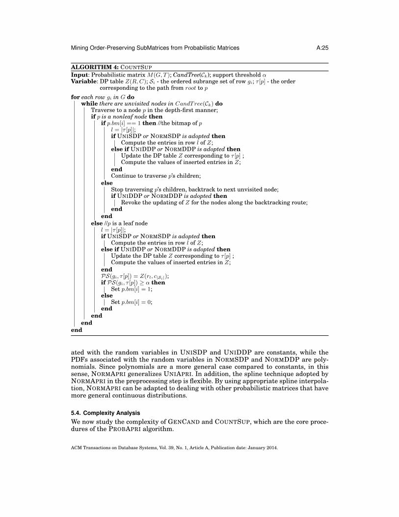
Mining Order-Preserving SubMatrices from Probabilistic Matrices A:25
ALGORITHM 4: COUNTSUP
Input: Probabilistic matrix M(G,T ); CandTree(Ck); support threshold αVariable: DP table Z(R,C); Si - the ordered subrange set of row gi; τ [p] - the order
corresponding to the path from root to pfor each row gi in G do
while there are unvisited nodes in CandTree(Ck) doTraverse to a node p in the depth-first manner;if p is a nonleaf node then
if p.bm[i] == 1 then //the bitmap of pl = |τ [p]|;if UNISDP or NORMSDP is adopted then
Compute the entries in row l of Z;else if UNIDDP or NORMDDP is adopted then
Update the DP table Z corresponding to τ [p] ;Compute the values of inserted entries in Z;
endContinue to traverse p’s children;
elseStop traversing p’s children, backtrack to next unvisited node;if UNIDDP or NORMDDP is adopted then
Revoke the updating of Z for the nodes along the backtracking route;end
endelse //p is a leaf node
l = |τ [p]|;if UNISDP or NORMSDP is adopted then
Compute the entries in row l of Z;else if UNIDDP or NORMDDP is adopted then
Update the DP table Z corresponding to τ [p] ;Compute the values of inserted entries in Z;
endPS(gi, τ [p]) = Z(rl, c|Si|);if PS(gi, τ [p]) ≥ α then
Set p.bm[i] = 1;else
Set p.bm[i] = 0;end
endend
end
ated with the random variables in UNISDP and UNIDDP are constants, while thePDFs associated with the random variables in NORMSDP and NORMDDP are poly-nomials. Since polynomials are a more general case compared to constants, in thissense, NORMAPRI generalizes UNIAPRI. In addition, the spline technique adopted byNORMAPRI in the preprocessing step is flexible. By using appropriate spline interpola-tion, NORMAPRI can be adapted to dealing with other probabilistic matrices that havemore general continuous distributions.
5.4. Complexity AnalysisWe now study the complexity of GENCAND and COUNTSUP, which are the core proce-dures of the PROBAPRI algorithm.
ACM Transactions on Database Systems, Vol. 39, No. 1, Article A, Publication date: January 2014.

A:26 Q. Fang et al.
1e+00
1e+02
1e+04
1e+06
1e+08
1e+10
1e+12
2 3 4 5 6 7 8
Num
ber
of o
rder
s
Round
#candidates(bp)#candidates(ap)
#frequentUpperBound
(a) α = 0.2
1e+00
1e+02
1e+04
1e+06
1e+08
1e+10
1e+12
2 3 4 5 6 7
Num
ber
of o
rder
s
Round
#candidates(bp)#candidates(ap)
#frequentUpperBound
(b) α = 0.4
Fig. 7. The effectiveness of GENCAND in controlling the number of candidate orders
The computational cost of the Apriori-based methods is not likely to be well boundeddue to the possible exponential number of candidates generated during candidate gen-eration. For example, suppose, in an m-by-n probabilistic matrix, every possible size-cmin order of columns is supported by at least rmin rows. Then, at the kth round ofcandidate generation with 1 < k ≤ cmin, no size-k order can be pruned by the GEN-CAND procedure since all its size-(k− 1) sub-orders are frequent. The number of size-kcandidate orders generated by GENCAND is n!
(n−k)! , and it is the upper-bound of thenumber of candidate orders that can be generated at the kth round. However, such anextreme case rarely happens in real application data, and the Apriori-based methodsare usually shown to be practically efficient [Aggarwal et al. 2009; Fang et al. 2012].Therefore, we conduct an experiment using a real dataset to study the effectiveness ofthe GENCAND procedure in controlling the number of candidate orders. We use a Uni-Dist matrix with 205 rows and 20 columns. It is converted from a real yeast dataset byadopting the Std method with the approximation range set to [µ−σ, µ+σ]. The matrixconversion methods are explained in detail in Section 6.1. The POPSM patterns withat least 60 rows and 5 columns are mined from the UniDist matrix with the supportthreshold α respectively set to 0.2 and 0.4. Given a data matrix with 20 columns, theupper-bound of the number of candidate orders that can be generated at the kth roundof candidate generation is 20!
(20−k)! . Figures 7(a) and 7(b) show the numbers of the can-didate orders generated by GENCAND before and after the pruning step, the numberof frequent orders, and the corresponding upper-bound at each round under two α set-tings. The series “#candidates (bp)” and “#candidates (ap)” respectively correspond tothe number of candidate orders before and after pruning.
When α equals 0.2, the mining process requires eight rounds as shown in Figure 7(a).At all the rounds, the number of candidate orders after pruning is no more than 4.5times the number of frequent orders, and it is several orders of magnitude fewer thanthe corresponding upper-bound starting from the fifth round. At the fourth round, thenumbers of candidate orders before and after pruning both reach the maximum, whichare respectively 6 times and 3 times the number of frequent orders in the same round.The number of candidate orders before pruning becomes about 50 times the numberof frequent orders at the seventh round, which seems to be a big difference. However,the absolute numbers of those candidate orders and frequent orders both decreasesubstantially in the last several rounds. In addition, the pruning step is efficient, which
ACM Transactions on Database Systems, Vol. 39, No. 1, Article A, Publication date: January 2014.

Mining Order-Preserving SubMatrices from Probabilistic Matrices A:27
reduces the number candidate orders to only 4.5 times the number of frequent orders.Similar results can be observed when α equals 0.4. Therefore, GENCAND is efficient incontrolling the number of candidate orders during candidate generation.
At the kth round of candidate verification, the COUNTSUP procedure needs to tra-verse the CandTree of Ck for m times, where m is the number of rows in the inputmatrix. Since each node in CandTree is visited for at most one time in one traversal,at most km|Ck| nodes are visited where |Ck| is the size of the set Ck. When a tree nodeis visited, one of the four DP methods is invoked to update their respective DP tables.We have respectively illustrated the time complexity of the four DP methods in Section5.3. For ease of presentation, we summarize in Table IV the computational cost of thefour DP methods at each node visit, and accordingly compute the cost of COUNTSUP atthe kth round. Although the time complexity of COUNTSUP contains up to the fourthpower of k which seems time-consuming, k is the size of the candidate orders and thusis usually a small value. Therefore, COUNTSUP is still practically efficient.
Table IV. Time complexity of COUNTSUP corresponding to four DP methods
DP Method Cost of DP process at a node visit Cost of COUNTSUP at the kth round
UNISDP O(kn) O(k2mn|Ck|)
UNIDDP O(k2) O(k3m|Ck|)
NORMSDP O(k2n) O(k3mn|Ck|)
NORMDDP O(k3) O(k4m|Ck|)
6. EXPERIMENTSIn this section, we study the performance of the POPSM model and the PROBAPRIframework on both synthetic datasets and real datasets. For clarity in our result pre-sentation, we denote the POPSM model by U-POPSM for the UniDist matrix and byN-POPSM for the NormDist matrix, and compare these two POPSM models with theOPSMRM model [Chui et al. 2008; Yip et al. 2013] and the OPSM model [Ben-Dor et al.2002]. We also compare the POPSM mining methods with that of OPSMRM. By set-ting the number of replicates to be 1, we employ the OPSMRM mining method to mineOPSM patterns. We implement the more efficient HT-Bound as the pruning strategyfor the OPSMRM mining method. All the algorithms are implemented in C++, and allthe experiments are conducted on a Macbook Pro with 2.53GHZ CPU and 4G memory.
6.1. Data PreparationThree real datasets are used in our experiments: a yeast galactose dataset [Idekeret al. 2001; Yeung et al. 2003] (or simply the yeast dataset), a rat circadian dataset[Nguyen et al. 2010] (or simply the rat dataset), and an RFID user trace dataset1 (orsimply the RFID dataset).
The yeast dataset contains 205 genes and 20 experimental conditions, and there arefour replicates for each entry of the matrix. This set-valued matrix has been used formining OPSMRM patterns. We generate a real-valued matrix by taking the averageof the four replicates of an entry as the new single entry value, and the generatedmatrix is taken as input for mining OPSM patterns. We adopt two methods to convertthe original set-valued matrix into a UniDist matrix. First, we set the range of everyentry by taking the smallest and largest values of the four replicates as the lower andupper bounds, which we call the MinMax method. Second, we compute the mean µ and
1http://lahar.cs.washington.edu/displayPage.php?path=./content/Download/RFIDData/rfidData.html
ACM Transactions on Database Systems, Vol. 39, No. 1, Article A, Publication date: January 2014.
A:28 Q. Fang et al.
the standard deviation σ based on the replicates of every entry and set the range to[µ − t ∗ σ, µ + t ∗ σ] where t is set to 1, 2, or 3, and we call this the Std method. Byusing the Std method, we expect the range covers the distribution of true replicatesand reduces the influence of possibly noisy ones. To generate the NormDist matrix, wecompute the mean and standard deviation of an entry based on the replicates. Duringthe cubic spline approximation, the approximation range is set to be [µ− t ∗ σ, µ+ t ∗ σ]and the range is divided into q pieces, where t is set to the values in {1, 2, 3} and q isset to the values in {4, 6, 8, 10}.
The rat dataset contains 527 genes and 10 conditions, and it is extracted using two-sample t-test from a larger dataset, which is collected by examining the fluctuation ofgene expressions in the rat livers within the 24 hour circadian cycle. It is also a set-valued matrix, and the number of replicates under a condition varies from 2 to 6. Weadopt the same method used in the yeast dataset to convert the rat dataset into theUniDist matrix and the NormDist matrix.
The RFID dataset contains the traces of twelve voluntary users in a building with195 RFID antennas installed. Only 44 antennas are active, that is, they detect thetrace of at least one user for at least one time. The trace of a user consists of a seriesof (period, antenna) pairs which indicates the time period during which the user iscontinuously detected by the antenna. When a user is detected by the same antennaat different time periods, we split the raw trace into several new traces in which theuser is detected by any antenna for at most one time. We then generate a UniDistmatrix having 103 rows (i.e., user traces) and 44 columns (i.e., antennas). The set oftimestamps within each time period is enumerated to generate the corresponding set-valued matrix, and the middle time points are computed to generate the real-valuedmatrix.
The synthetic datasets are generated based on the real yeast dataset. To generatean r-by-c matrix, we first randomly pick r rows and c columns from the original matrixand generate an r-by-c set-valued matrix. To simulate randomness, each entry in thematrix is shifted left or right with a small constant, or is kept unchanged with equalprobability. Then, similar methods used for the real datasets are employed to convertthe set-valued matrix into the UniDist or NormDist matrix.
6.2. Evaluation MeasuresWe now explain the methodology of evaluating the experimental results. There arethree evaluation measures, namely the biological significance of the patterns minedfrom the biological datasets, the trace accuracy score of the patterns mined from theRFID dataset, and the running time for mining patterns in general.
6.2.1. Biological Significance. To compare the effectiveness of different models that pro-mote the discovery of interesting patterns from gene expression data, we validate thebiological significance of the POPSM, OPSMRM, and OPSM patterns mined from thetwo biological datasets. We adopt a measurement called p-value [Zhang et al. 2008;Fang et al. 2010; Fang et al. 2012], which is well accepted for measuring the associ-ation between mined patterns and the known gene functional categories. Essentially,a smaller p-value indicates a stronger association between a pattern and some genecategory, and the pattern is thus regarded as more biologically significant.
6.2.2. Trace Accuracy. The patterns mined from the RFID dataset consists of a set ofusers sharing a common subroute passing a subset of antennas. To evaluate whetherthe subroute really matches the ground-truth traces of the users, we define a measurecalled the trace accuracy score and denote this score by S(P,Q, τQ) where (P,Q : τQ)is a POPSM, an OPSMRM or an OPSM pattern having τQ as the backbone order. The
ACM Transactions on Database Systems, Vol. 39, No. 1, Article A, Publication date: January 2014.

Mining Order-Preserving SubMatrices from Probabilistic Matrices A:29
trace accuracy score of a pattern (P,Q : τQ) is computed as follows.
S(P,Q, τQ) =1
|P |∑gi∈P
|LCS(τQ, Tgi)||τQ|
,
where Tgi is the ground-truth trace of user gi, and |LCS(τQ, Tgi)| is the length of thelongest common subsequence between the detected subroute τQ and Tgi . The introduc-tion of the two normalized factors |P | and |τQ| in the score function makes the scoresof patterns with different sizes comparable.
6.2.3. Efficiency. We study the efficiency of different methods by comparing their run-ning times in two ways. First, we denote by TR-Time the total running time for gener-ating the patterns. Second, we also study the average time for mining a single pattern,which is denoted by SP-Time, since the number of patterns mined by one method orunder one setting is not the same as that mined by another method or under anothersetting in general.
6.3. Comparison of Data Conversion MethodsGiven a set-valued matrix, we use the MinMax or Std methods described in Section6.1 to convert it to a UniDist or a NormDist matrix. In the first set of experiments,we use the yeast dataset to study the impact of conversion methods on the quality ofmined U-POPSM and N-POPSM patterns. The DDP technique is adopted for both theUNIAPRI and NORMAPRI methods.
When the Std method is taken for generating the UniDist matrix, the parametert for the approximation range [µ − t ∗ σ, µ + t ∗ σ] is additionally set to 1, 2, and 3.Including the UniDist matrix generated by MinMax, there are four UniDist matricesgenerated by different methods or under different settings. Based on each UniDistmatrix, the UNIAPRI method is employed to mine U-POPSM patterns containing atleast 60 rows and 5 columns, and having α = 0.3. We set four p-value ranges which are[1e−20,++), [1e−30, 1e−20), [1e−40, 1e−30) and [0, 1e−40), and call them significancelevels. If the p-value of a pattern falls within any range, we say that the pattern reachesthe corresponding significance level. Figure 8(a) shows the fractions of patterns thatare mined from different UniDist matrices and reach different significance levels. Thebar labeled “MinMax” in the figure corresponds to the statistics of the patterns minedfrom the UniDist matrix generated by the MinMax method, and the bar labeled “±1σ”corresponds to the statistics of the patterns mined from the UniDist matrix generatedby the Std method with t = 1. In all the series, the white color is used to show the frac-tion of the most significant patterns whose p-values fall within the highest significancelevel [0, 1e− 40).
Among the patterns mined under the settings “MinMax” and “±1σ”, about 30% ofthe patterns have the p-values smaller than 1e− 40, which means that they reach thehighest significance level [0, 1e−40). In contrast, only 15% of the patterns mined underthe setting “±2σ” reach the same level, and no pattern mined under the setting “±3σ”reaches this significance level. A possible explanation is that the approximation range[µ − tσ, µ + tσ] with t ≥ 2 is too large, which covers not only the true replicates butalso the noisy ones. Under the uniform distribution model, both the true replicatesand the noisy ones are associated with equally large probability densities, and thusthe quality of mined patterns are affected due to the coverage of noisy replicates bya larger approximation range. Although the quality of the patterns mined under thesetting “±1σ” and that of the patterns mined under the setting “MinMax” are verysimilar, the fraction of patterns that are mined under the setting “±1σ” and reach thehighest significance level, i.e., 31.2%, is slightly larger than that of patterns that aremined under “MinMax” and reach the same level, i.e., 29.9%. Besides, slightly larger
ACM Transactions on Database Systems, Vol. 39, No. 1, Article A, Publication date: January 2014.
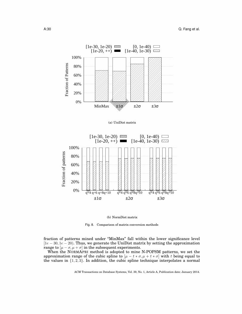
A:30 Q. Fang et al.
0%
20%
40%
60%
80%
100%
MinMax ±1σ ±2σ ±3σ
Frac
tion
of P
atte
rns
[1e-20, ++)[1e-30, 1e-20)
[1e-40, 1e-30)[0, 1e-40)
(a) UniDist matrix
0%
20%
40%
60%
80%
100%
q=4 q=6 q=8q=10 q=4 q=6 q=8q=10 q=4 q=6 q=8q=10
Frac
tion
of p
atte
rns
[1e-20, ++)[1e-30, 1e-20)
[1e-40, 1e-30)[0, 1e-40)
±3σ±2σ±1σ
(b) NormDist matrix
Fig. 8. Comparison of matrix conversion methods
fraction of patterns mined under “MinMax” fall within the lower significance level[1e − 30, 1e − 20). Thus, we generate the UniDist matrix by setting the approximationrange to [µ− σ, µ+ σ] in the subsequent experiments.
When the NORMAPRI method is adopted to mine N-POPSM patterns, we set theapproximation range of the cubic spline to [µ − t ∗ σ, µ + t ∗ σ] with t being equal tothe values in {1, 2, 3}. In addition, the cubic spline technique interpolates a normal
ACM Transactions on Database Systems, Vol. 39, No. 1, Article A, Publication date: January 2014.
Mining Order-Preserving SubMatrices from Probabilistic Matrices A:31
distribution with q polynomials, where q is set to the values in {4, 6, 8, 10}. For differentcombinations of t and q values, we adopt the NORMAPRI method to mine N-POPSMpatterns that contain at least 60 rows and 5 columns and satisfy the support thresholdα = 0.3. The statistics on the quality of the mined patterns are shown in Figure 8(b),where the bar labeled “±1σ, q=4” corresponds to the results with the approximationrange [µ − σ, µ + σ] and four intervals in the spline approximation. Again, comparingthe three settings of the approximation range, a larger fraction of mined patterns reachthe highest significance level when the approximation range is [µ−σ, µ+σ]. The reasonis similar to that for the UniDist matrix: a larger approximation range is more likelyto cover many noisy replicates, which accordingly influences the quality of the minedpatterns. With the approximation range fixed, the setting of q does not influence thequality of the mined patterns. For example, when the approximation range is set to [µ−σ, µ+ σ], no matter what q value is, 32% of the patterns reach the highest significancelevel, and 1% of the patterns reach the significance level of [1e− 30, 1e− 20). However,a larger q implies that a normal distribution is interpolated with more polynomials,which accordingly influences the efficiency of the NORMAPRI method. Therefore, wechoose [µ−σ, µ+σ] to be the approximation range for the NormDist matrix and alwaysset q to 4 in the experiments discussed in subsequent sections.
Comparing these two types of the probabilistic matrices, the quality of the N-POPSMpatterns mined from the NormDist matrix is less affected by the conversion methodsand the settings. For example, when the approximation range is [µ− σ, µ+ σ], the per-centage of the U-POPSM and N-POPSM patterns that reach the highest significancelevel are both around 30%. When the approximation range is [µ − 3σ, µ + 3σ], thereare still about 25% of the N-POPSM patterns reaching the highest significance level,while no U-POPSM pattern reaches the same level. The reason is that, although alarger approximation range may cover more noisy replicates in the NormDist matrix,these noisy values are usually farther away from the mean of the range, and so theyare associated with very small probability densities. The influence of such noisy valuesto the computation of probabilistic support is then limited, and the quality of minedN-POPSM patterns can be well maintained. In the UniDist matrix, a larger approx-imation range also covers more noisy replicates, which however are associated withequally large probabilities as the true replicates. The inclusion of the noisy replicatesaffects the accuracy of the probabilistic supports of rows w.r.t. orders, and accordinglydegrades the quality of mined U-POPSM patterns. Therefore, compared to the UniDistmatrix, the NormDist matrix well smoothes out the influence of noisy replicates to thequality of mined patterns, and better models the noisy scientific data like the yeastdataset we are using. However, by carefully choosing the conversion method as wellas the approximation range when generating the UniDist matrix, the quality of theU-POPSM patterns can still be maintained.
6.4. Scalability of PROBAPRI
In this set of experiments, we use the synthetic datasets to study the efficiency of theUNIAPRI and NORMAPRI methods w.r.t. the size of the input matrix. As both methodscan adopt either the SDP or the DDP technique for candidate verification, we comparethe TR-Time and SP-Time of each method using the two DP techniques. Following theconvention introduced in Table III, we denote the UNIAPRI method with the static(or respectively the dynamic) DP technique by UNISDP (or respectively UNIDDP),and denote the NORMAPRI method with the static (or respectively the dynamic) DPtechnique by NORMSDP (or respectively NORMDDP).
First, we set the number of columns c to 15 and 20, vary the number of rows withthe values in {200, 400, 600, 800, 1000}, and adopt the Std method described in Section6.1 to generate r-by-c UniDist matrices. The approximation range is set to [µ−σ, µ+σ].
ACM Transactions on Database Systems, Vol. 39, No. 1, Article A, Publication date: January 2014.
A:32 Q. Fang et al.
0
10
20
30
40
50
200 400 600 800 1000
TR
-Tim
e (s
ec)
Number of rows
UniSDP, c=15UniSDP, c=20UniDDP, c=15UniDDP, c=20
(a) TR-Time w.r.t. r
0
0.0005
0.001
0.0015
0.002
200 400 600 800 1000
SP-T
ime
(sec
)
Number of rows
UniSDP, c=15UniSDP, c=20UniDDP, c=15UniDDP, c=20
(b) SP-Time w.r.t. r
0
20
40
60
80
100
120
10 15 20 25 30
TR
-Tim
e (s
ec)
Number of columns
UniSDP, r=200UniSDP, r=400UniDDP, r=200UniDDP, r=400
(c) TR-Time w.r.t. c
0
0.002
0.004
0.006
0.008
0.01
10 15 20 25 30
SP-T
ime
(sec
)
Number of columns
UniSDP, r=200UniSDP, r=400UniDDP, r=200UniDDP, r=400
(d) SP-Time w.r.t. c
Fig. 9. Running time w.r.t. the size of a UniDist matrix
Then, the UNIAPRI method is adopted to mine U-POPSM patterns. The size thresholdrmin is set to 10%×r, and cmin is varied from 4 to 8 as the number of columns increasesfrom 10 to 30 in order to control the number of patterns. The support threshold α isfixed to 0.3. Figures 9(a) and 9(b) show the TR-Time and SP-Time of UNISDP andUNIDDP w.r.t. the number of rows in the input UniDist matrix. Then, we set thenumber of rows r to 200 and 400, and generate the UniDist matrices by varying thenumber of columns with the values in {10, 15, 20, 25, 30}. Figures 9(c) and 9(d) show theTR-Time and SP-Time of UNISDP and UNIDDP w.r.t. the number of columns in theinput matrix.
From Figure 9(a), we find that both the UNISDP and the UNIDDP methods scalewell w.r.t. the number of rows in the UniDist matrix. Specifically, when the numberof columns c is fixed to 15 and the number of rows increases by 5 times, from 200 to1000, the TR-time increases linearly, from 1.4 to 6.6 seconds for UNISDP and from 1.8to 8.3 seconds for UNIDDP. The same trend is observed again in Figure 9(b), wherethe SP-Time of the two methods is compared. Notably, UNISDP and UNIDDP arevery efficient in mining U-POPSM patterns, and both take less than 0.0015 secondsfor mining a pattern from a UniDist matrix having 1000 rows and 20 columns. Incomparison, these two methods are more affected by the number of columns in the
ACM Transactions on Database Systems, Vol. 39, No. 1, Article A, Publication date: January 2014.

Mining Order-Preserving SubMatrices from Probabilistic Matrices A:33
0
200
400
600
800
1000
1200
200 400 600 800 1000
TR
-Tim
e (s
ec)
Number of rows
NormSDP, c=15NormSDP, c=20NormDDP, c=15NormDDP, c=20
(a) TR-Time w.r.t. r
0
0.01
0.02
0.03
0.04
200 400 600 800 1000
SP-T
ime
(sec
)
Number of rows
NormSDP, c=15NormSDP, c=20NormDDP, c=15NormDDP, c=20
(b) SP-Time w.r.t. r
0e+00
2e+03
4e+03
6e+03
8e+03
10 15 20 25 30
TR
-Tim
e (s
ec)
Number of columns
NormSDP, r=200NormSDP, r=400NormDDP, r=200NormDDP, r=400
(c) TR-Time w.r.t. c
0
0.1
0.2
0.3
0.4
10 15 20 25 30
SP-T
ime
(sec
)
Number of columns
NormSDP, r=200NormSDP, r=400NormDDP, r=200NormDDP, r=400
(d) SP-Time w.r.t. c
Fig. 10. Running time w.r.t. the size of NormDist matrix
input matrix, as shown in Figures 9(c) and 9(d). The reason is that, an increase of thenumber of columns results in an increase of the number of candidate orders during thecandidate generation step and, thus, more time is needed to generate and verify thecandidate orders.
Comparing UNISDP and UNIDDP, we find that UNISDP is slightly more efficientthan UNIDDP. The advantage of UNISDP is more apparent when the number ofcolumns in the matrix is smaller. The reason is that, the DP process needed for can-didate verification is already very efficient for the UniDist matrix. Although the DDPtechnique adopted by UNIDDP is designed to reduce the size of the DP table andlower the time cost incurred by the DP process, dynamically updating the DP tabletakes extra time. Therefore, not much time can be saved eventually. However, whenthe number of columns in the input matrix is large enough, the DDP technique is ben-eficial. For example, when r equals 200 and c equals 30, the TR-Time and SP-Timeof UNISDP are respectively 52.17 and 0.0039 seconds, while those of UNIDDP arerespectively 47.06 and 0.0035 seconds. Since the performance of these two versionsare comparable and both are efficient, we choose the DDP version of UNIAPRI in thesubsequent experiments.
ACM Transactions on Database Systems, Vol. 39, No. 1, Article A, Publication date: January 2014.

A:34 Q. Fang et al.
To study the scalability of the NORMAPRI method, we adopt the Std method to gen-erate the NormDist matrix with settings t = 1 and q = 4. The number of rows r andthe number of columns c are varied in the same way as they are for generating theUniDist matrix. When the N-POPSM patterns are mined, the size thresholds rmin isset to 10% × r, cmin is varied from 4 to 8, and the support threshold α is fixed to 0.3.Figure 10 shows the TR-Time and SP-Time of NORMSDP and NORMDDP w.r.t. thesize of the input NormDist matrix.
Similarly to the two versions of UNIAPRI, both NORMSDP and NORMDDP scalewell as the number of rows in the input matrix increases, and they are more affected bythe number of columns. Referring to Figures 10(a) and 10(b), we can see that, when thenumber of rows increases from 200 to 1000, the TR-Time and SP-Time of NORMSDPand NORMDDP all linearly increase by about 5 times. However, Figure 10(d) showsthat, as the number of columns increases from 10 to 30, the SP-Time of NORMSDPincreases by about 30 times while the SP-Time of NORMDDP increases by about 10times. As the DP process in NORMAPRI is time-consuming, the adoption of the DDPtechnique greatly improves the efficiency of mining N-POPSM patterns, and the ad-vantage becomes more apparent when r or c gets larger. When c is 30, the TR-Timeof NORMDDP is 33% of the TR-Time of NORMSDP with r = 20 and is only 22% withr = 40. The saving of the SP-Time is also up to 70%.
Note that, no matter which DP technique is taken in the UNIAPRI method, thenumber of patterns mined from the same UniDist matrix is the same. However, due tothe computation error of cubic polynomial integral, the number of patterns mined byNORMAPRI using different DP techniques is slightly different. The difference is lessthan 0.3%, that is, the number of patterns differs by 3 for every 1000 patterns. Sincethe difference is not significant, we adopt the more efficient NORMDDP in NORMAPRIin the subsequent experiments.
6.5. Experiments on the Yeast DatasetIn this set of experiments, we use the yeast dataset to study the effectiveness of thePOPSM model for discovering significant patterns. We study the settings of the pa-rameters, such as the size thresholds rmin and cmin, and the support threshold α. Thebiological significance of the U-POPSM and N-POPSM patterns is compared with thatof the OPSMRM and OPSM patterns. The efficiency of the corresponding mining meth-ods is also studied.
6.5.1. Influence of the size thresholds. For real datasets, it is difficult to determine propervalues for the two size thresholds rmin and cmin such that the patterns satisfying thethresholds are all guaranteed to have good quality. Ben-Dor et al. brought forwarda heuristic solution to this problem [Ben-Dor et al. 2002]. Since patterns with largersize are statistically less likely to exist by random in a data matrix, these statisticallysignificant patterns are more probable to reveal important knowledge hidden in thematrix, and thus should also be biologically significant. Therefore, in order to guaran-tee the quality of mined patterns, we prefer patterns with larger size. Suppose thereis a random real-valued matrix having 205 rows and 20 columns, which is the samesize as the yeast dataset. Since the number of possible orders of 3 columns is 3! = 6,we should always be able to find an OPSM pattern with 3 columns and 205
6 ≈ 34 rows,and so this pattern is of low statistical significance. To guarantee the quality of thepatterns mined from the yeast dataset, we set the size thresholds to be larger than 34rows and 3 columns.
We study the influence of the size thresholds to the quality of the patterns by fixingα to 0.3, and varying rmin with the values in {40, 50, 60, 70} and varying cmin with thevalues in {4, 5, 6}. Due to space limit, we only present the results with rmin equal to
ACM Transactions on Database Systems, Vol. 39, No. 1, Article A, Publication date: January 2014.
Mining Order-Preserving SubMatrices from Probabilistic Matrices A:35
0%
20%
40%
60%
80%
100%
(40,4)
(40,5)
(40,6)
(60,4)
(60,5)
(60,6)
(40,4)
(40,5)
(40,6)
(60,4)
(60,5)
(60,6)
(40,4)
(40,5)
(40,6)
(60,4)
(60,5)
(60,6)
(40,4)
(40,5)
(40,6)
(60,4)
(60,5)
(60,6)
Frac
tion
of p
atte
rns
(rmin, cmin) and pattern types
[1e-20, ++)
[1e-30, 1e-20)
[1e-40, 1e-30)
[0, 1e-40)
OPSMOPSMRMN-POPSMU-POPSM
(a) Fraction of patterns w.r.t. the size thresholds
0.0e+00
1.0e+04
2.0e+04
3.0e+04
(40,4) (40,5) (40,6) (60,4) (60,5) (60,6)
Num
ber
of p
atte
rns
(rmin, cmin)
U-POPSMN-POPSMOPSMRM
OPSM
(b) Number of patterns w.r.t. the size thresholds
Fig. 11. Influence of the size thresholds cmin and rmin
40 and 60. Similarly to the first set of experiments, we also set four significance levels.Figure 11(a) shows the fraction of patterns that respectively reach each significancelevel. The first bar “(40, 4), U-POPSM” corresponds to the distribution of the U-POPSMpatterns mined by UNIAPRI with rmin and cmin respectively set to 40 and 4. We can
ACM Transactions on Database Systems, Vol. 39, No. 1, Article A, Publication date: January 2014.

A:36 Q. Fang et al.
see that, when rmin is smaller than or equal to 50, for all the four pattern types, thereare around 40–90% of the mined patterns falling within the two lowest significancelevels. The quality of the mined patterns however improves substantially when rmin islarger than or equal to 60. Especially when cmin is larger than or equal to 5, less than1% of the U-POPSM and N-POPSM paterns, about 2% of the OPSMRM patterns, and2.5% of the OPSM patterns fall within the two lowest significance levels. On the otherhand, the number of mined patterns decreases a lot when rmin and cmin get larger, asshown in Figure 11(b). When rmin equals 60 and cmin equals 6, around 470 U-POPSMand N-POPSM patterns have been mined, but only 11 OPSMRM patterns have beenmined. To achieve a good balance between pattern quality and pattern number, wetherefore respectively set rmin and cmin to 60 and 5 in the experiments.
6.5.2. Influence of the support threshold. As a larger probabilistic support (or fractionalsupport used by the OPSMRM model) value intuitively implies a better or more per-suasive support of a row w.r.t. an order. When mining the POPSM or OPSMRM pat-terns, a support threshold α is needed to exclude those rows whose support to a certainorder is too small to be meaningful. Similarly to the setting of the size thresholds, thesetting of α should ideally be determined by the noise level of the datasets. However,such prior knowledge about the real datasets is usually not available. Therefore, weempirically study the influence of the support threshold to the quality of mined pat-terns.
We fix the size thresholds rmin and cmin to 60 and 5, and vary α from 0.1 to 0.5for UNIAPRI, NORMAPRI, and the OPSMRM mining method. The OPSMRM miningmethod is also employed for mining the OPSM patterns with α = 1. The statistics onthe biological significance of the patterns are shown in Figures 12(a) and 12(b). Fig-ure 12(a) shows the fractions of patterns that reach the four significance level. Forall U-POPSM, N-POPSM, and OPSMRM patterns, the fraction of the most significantpatterns generally increases as α decreases, and the best result for each model is ob-tained when α equals 0.2. With the same α value, the fractions of the most significantU-POPSM and N-POPSM patterns are apparently larger than that of the most signifi-cant OPSMRM patterns, and the fraction of such N-POPSM patterns is slightly largerthan that of the U-POPSM patterns. On the other hand, less than 0.06% of U-POPSMand N-POPSM patterns fall within the lowest significance level, while about 10% ofOPSMRM patterns fall within this level. If we consider the absolute number of pat-terns as shown in Figure 12(b), the advantage of the U-POPSM and N-POPSM modelsbecomes very clearly. When α is 0.2, 3112 U-POPSM patterns and 3004 N-POPSMpatterns reach the highest significance level, while only 915 OPSMRM patterns and735 OPSM patterns reach the same level.
We observe that PROBAPRI mines a large fraction of the most significant POPSMpatterns but still keeps the fraction of the least significant ones small. This fact againconfirms the superiority of our probabilistic matrix representation compared to theset-valued matrix representation. In the set-valued matrix, a small setting of α like0.2 promotes the discovery of the most significant patterns. However, the noisy repli-cates, which have an equally large probability as the true replicates, may result inthat uncorrelated rows also satisfy the small threshold and thus are included in manypatterns. The quality of these patterns are degraded, and the fraction of the least sig-nificant patterns accordingly becomes larger. In contrast, when we convert the yeastdataset to a NormDist matrix, noisy replicates that are usually far away from themean of the approximation range are associated with small probability densities, andthus their effect to the computation of the probabilistic support is limited. As the prob-abilistic support based on the NormDist matrix more accurately reflects the supportsof rows w.r.t. orders, the quality of mined N-POPSM patterns are well maintained. By
ACM Transactions on Database Systems, Vol. 39, No. 1, Article A, Publication date: January 2014.

Mining Order-Preserving SubMatrices from Probabilistic Matrices A:37
0%
20%
40%
60%
80%
100%
0.50.40.30.20.1 0.50.40.30.20.1 0.50.40.30.20.1
Frac
tion
of p
atte
rns
α and pattern types
[1e-20, ++)
[1e-30, 1e-20)
[1e-40, 1e-30)
[0, 1e-40)
OPSMOPSMRMN-POPSMU-POPSM
(a) Fraction of patterns at four significance levels
0.0e+00
5.0e+03
1.0e+04
1.5e+04
2.0e+04
2.5e+04
3.0e+04
0.50.40.30.20.1 0.50.40.30.20.1 0.50.40.30.20.1
Num
ber
of p
atte
rns
α and pattern types
[1e-20, ++)
[1e-30, 1e-20)
[1e-40, 1e-30)
[0, 1e-40)
OPSMOPSMRMN-POPSMU-POPSM
(b) Number of patterns at four significance levels
Fig. 12. Distribution of the p-values of the patterns mined from the yeast data
carefully choosing the conversion method as well as the approximation range of theUniDist matrix, the influence of noisy replicates can be eliminated and the quality ofmined U-POPSM pattern are still well controlled.
Let us illustrate the biological significance of mined POPSM patterns with a specificcase. A U-POPSM pattern is mined when α is 0.2, which contains 82 genes and gets
ACM Transactions on Database Systems, Vol. 39, No. 1, Article A, Publication date: January 2014.
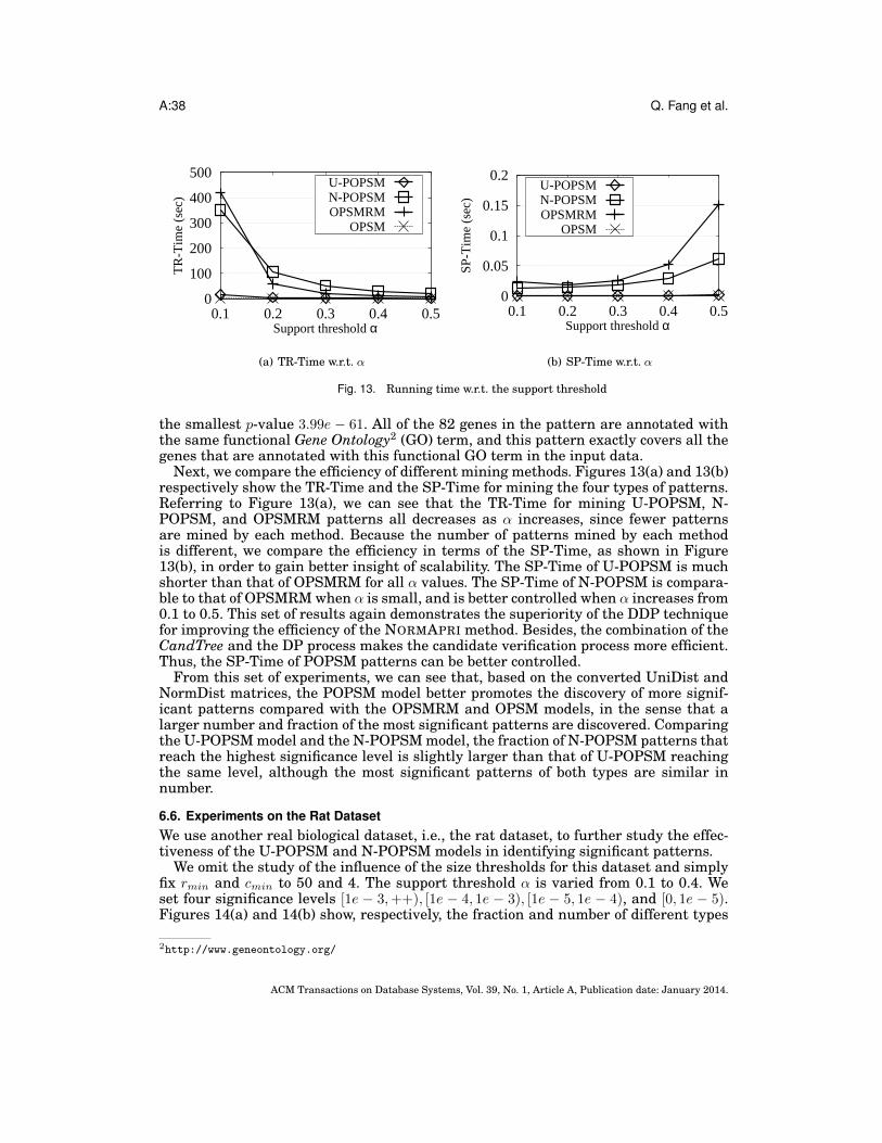
A:38 Q. Fang et al.
0
100
200
300
400
500
0.1 0.2 0.3 0.4 0.5
TR
-Tim
e (s
ec)
Support threshold α
U-POPSMN-POPSMOPSMRM
OPSM
(a) TR-Time w.r.t. α
0
0.05
0.1
0.15
0.2
0.1 0.2 0.3 0.4 0.5
SP-T
ime
(sec
)
Support threshold α
U-POPSMN-POPSMOPSMRM
OPSM
(b) SP-Time w.r.t. α
Fig. 13. Running time w.r.t. the support threshold
the smallest p-value 3.99e − 61. All of the 82 genes in the pattern are annotated withthe same functional Gene Ontology2 (GO) term, and this pattern exactly covers all thegenes that are annotated with this functional GO term in the input data.
Next, we compare the efficiency of different mining methods. Figures 13(a) and 13(b)respectively show the TR-Time and the SP-Time for mining the four types of patterns.Referring to Figure 13(a), we can see that the TR-Time for mining U-POPSM, N-POPSM, and OPSMRM patterns all decreases as α increases, since fewer patternsare mined by each method. Because the number of patterns mined by each methodis different, we compare the efficiency in terms of the SP-Time, as shown in Figure13(b), in order to gain better insight of scalability. The SP-Time of U-POPSM is muchshorter than that of OPSMRM for all α values. The SP-Time of N-POPSM is compara-ble to that of OPSMRM when α is small, and is better controlled when α increases from0.1 to 0.5. This set of results again demonstrates the superiority of the DDP techniquefor improving the efficiency of the NORMAPRI method. Besides, the combination of theCandTree and the DP process makes the candidate verification process more efficient.Thus, the SP-Time of POPSM patterns can be better controlled.
From this set of experiments, we can see that, based on the converted UniDist andNormDist matrices, the POPSM model better promotes the discovery of more signif-icant patterns compared with the OPSMRM and OPSM models, in the sense that alarger number and fraction of the most significant patterns are discovered. Comparingthe U-POPSM model and the N-POPSM model, the fraction of N-POPSM patterns thatreach the highest significance level is slightly larger than that of U-POPSM reachingthe same level, although the most significant patterns of both types are similar innumber.
6.6. Experiments on the Rat DatasetWe use another real biological dataset, i.e., the rat dataset, to further study the effec-tiveness of the U-POPSM and N-POPSM models in identifying significant patterns.
We omit the study of the influence of the size thresholds for this dataset and simplyfix rmin and cmin to 50 and 4. The support threshold α is varied from 0.1 to 0.4. Weset four significance levels [1e − 3,++), [1e − 4, 1e − 3), [1e − 5, 1e − 4), and [0, 1e − 5).Figures 14(a) and 14(b) show, respectively, the fraction and number of different types
2http://www.geneontology.org/
ACM Transactions on Database Systems, Vol. 39, No. 1, Article A, Publication date: January 2014.
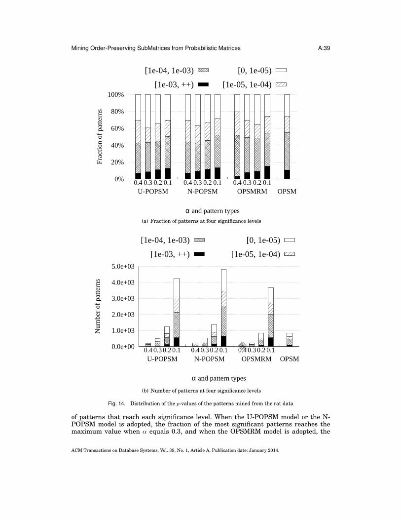
Mining Order-Preserving SubMatrices from Probabilistic Matrices A:39
0%
20%
40%
60%
80%
100%
0.4 0.3 0.2 0.1 0.4 0.3 0.2 0.1 0.4 0.3 0.2 0.1
Frac
tion
of p
atte
rns
α and pattern types
[1e-03, ++)
[1e-04, 1e-03)
[1e-05, 1e-04)
[0, 1e-05)
OPSMOPSMRMN-POPSMU-POPSM
(a) Fraction of patterns at four significance levels
0.0e+00
1.0e+03
2.0e+03
3.0e+03
4.0e+03
5.0e+03
0.4 0.3 0.2 0.1 0.4 0.3 0.2 0.1 0.4 0.3 0.2 0.1
Num
ber
of p
atte
rns
α and pattern types
[1e-03, ++)
[1e-04, 1e-03)
[1e-05, 1e-04)
[0, 1e-05)
OPSMOPSMRMN-POPSMU-POPSM
(b) Number of patterns at four significance levels
Fig. 14. Distribution of the p-values of the patterns mined from the rat data
of patterns that reach each significance level. When the U-POPSM model or the N-POPSM model is adopted, the fraction of the most significant patterns reaches themaximum value when α equals 0.3, and when the OPSMRM model is adopted, the
ACM Transactions on Database Systems, Vol. 39, No. 1, Article A, Publication date: January 2014.

A:40 Q. Fang et al.
20%
40%
60%
80%
100%
0.9 0.8 0.7 0.9 0.8 0.7
Frac
tion
of p
atte
rns
α and pattern types
[0.5, 0.7)
[0.7, 0.8)
[0.8, 0.9)
[0.9, 1.0]
OPSMOPSMRMU-POPSM
Fig. 15. Distribution of the accuracy score of the patterns mined from the RFID dataset
fraction of the most significant patterns reaches the maximum value when α equals0.2. Under the best setting for each model, larger fractions of U-POPSM and N-POPSMpatterns reach the highest significance level compared to the OPSMRM and OPSMpatterns. In addition, the fraction of the U-POPSM patterns that fall within the lowestsignificance level is the smallest among the four models. If the number of patterns thatreach the highest significance level is compared, both the U-POPSM and N-POPSMmodels outperform the OPSMRM model for all α values as well.
6.7. Experiments on the RFID DatasetIn the last set of experiments, we use the RFID dataset to evaluate the capability of thePOPSM model in revealing the common subroutes of the users. Since the RFID datasetis given as a UniDist matrix, we only study the effectiveness of the U-POPSM model.We convert the UniDist matrix to a set-valued matrix by enumerating the timestampswithin each range. We also convert the UniDist matrix to a real-valued matrix bytaking the middle time point of each range. We set rmin and cmin to 12 and 9, andmine U-POPSM, OPSMRM and OPSM patterns. Figure 15 shows the distribution ofthe accuracy scores of the patterns. For a particular pattern, the larger its score is,the more accurate it is at capturing the common subroute of the set of involved users.When mining U-POPSM and OPSMRM patterns, we vary α from 0.7 to 0.9. In termsof the fraction of patterns that fall into the highest score range [0.9, 1.0], both methodsachieve the best result when α equals 0.8. The reason may be that, a large setting ofα, say 0.8, would be too strict to tolerate intrinsic noise in RFID data, while settingα with a smaller value would obscure the true traces of the users. From Figure 15,we can see that, compared to the OPSMRM and OPSM patterns, a larger fraction ofU-POPSM patterns fall into the highest score range. Furthermore, the accuracy scoresof all the U-POPSM patterns are above 0.7, while more than 25% of the OPSMRM andOPSM patterns have the accuracy scores below 0.7.
ACM Transactions on Database Systems, Vol. 39, No. 1, Article A, Publication date: January 2014.

Mining Order-Preserving SubMatrices from Probabilistic Matrices A:41
7. CONCLUSIONSIn this paper, we study the problem of mining probabilistic OPSM patterns from un-certain data matrices having continuous distributions. We consider two representa-tive distributions, the uniform distribution and the normal distribution, and accord-ingly formulate the uncertain data as the UniDist matrix and the NormDist matrix.Compared to a set-valued matrix representation, our UniDist and NormDist matrixrepresentations better smooth out the influence of noise in real datasets. Based onthe UniDist and NormDist matrices, we propose a novel probabilistic OPSM (POPSM)model. We define a new probabilistic support measure that evaluates the extent towhich a row supports an order. The POPSM model uses a backbone order to capturea consensus trend, and all the rows in a POPSM pattern are required to support thebackbone order of the pattern with sufficiently large probabilistic support.
In order to mine POPSM patterns effectively and efficiently, we develop two newPOPSM mining methods: UNIAPRI for the UniDist matrix and NORMAPRI for theNormDist matrix. In both UNIAPRI and NORMAPRI, a prefix-tree structure calledCandTree is designed to organize the intermediate patterns in a compact way. Twonovel dynamic programming techniques, the static DP and the dynamic DP, are alsoexploited in our methods, and the DP computation process is interwoven with thetraversal of CandTree for efficient pattern verification.
We evaluate our POPSM mining approach on two real biological datasets, onereal RFID dataset, and several synthetic datasets. Our experiments on the biologi-cal datasets show that, comparing with the counterpart OPSMRM model, the POPSMmodel better captures the characteristics of the expression levels of biologically corre-lated genes, and greatly promotes the discovery of patterns with high biological sig-nificance. Through the experiments on the RFID data, the POPSM model is shown tobe capable of accuratly discovering users’ common subroutes from noisy trace data.The experiments on the synthetic datasets demonstrate the efficiency of the UNIAPRImethod. In particular, the dynamic DP technique greatly improves the efficiency of theNORMAPRI method.
Finally, it is worth noting that, while we study in depth two representative proba-bilistic distributions of uncertain data in this work, the spline technique adopted byNORMAPRI is flexible. By using appropriate spline interpolation, NORMAPRI can beadapted to dealing with other probabilistic matrices that have more general continu-ous distributions with high accuracy.
ACKNOWLEDGMENTS
The authors would like to thank the anonymous reviewers for their insightful comments.
REFERENCESAGGARWAL, C. C., LI, Y., WANG, J., AND WANG, J. 2009. Frequent pattern mining with uncertain data.
In Proceedings of the 15th ACM SIGKDD international conference on Knowledge discovery and datamining. KDD ’09. ACM, New York, NY, USA, 29–37.
AGGARWAL, C. C., WOLF, J. L., YU, P. S., PROCOPIUC, C., AND PARK, J. S. 1999. Fast algorithms forprojected clustering. In Proceedings of the ACM SIGMOD international conference on Management ofdata. SIGMOD ’99. ACM, New York, NY, USA, 61–72.
AGRAWAL, R., GEHRKE, J., GUNOPULOS, D., AND RAGHAVAN, P. 1998. Automatic subspace clustering ofhigh dimensional data for data mining applications. In Proceedings of the ACM SIGMOD internationalconference on Management of data. SIGMOD ’98. ACM, New York, NY, USA, 94–105.
AGRAWAL, R. AND SRIKANT, R. 1995. Mining sequential patterns. In Proceedings of the IEEE 11th Inter-national Conference on Data Engineering. ICDE ’95. IEEE Computer Society, Washington, DC, USA,3–14.
AHSANULLAH, M., NEVZOROV, V., AND SHAKIL, M. 2013. An Introduction to Order Statistics. AtlantisStudies in Probability and Statistics Series, vol. 3. Atlantis Press.
ACM Transactions on Database Systems, Vol. 39, No. 1, Article A, Publication date: January 2014.
A:42 Q. Fang et al.
BANERJEE, A., DHILLON, I., GHOSH, J., MERUGU, S., AND MODHA, D. S. 2004. A generalized maximumentropy approach to bregman co-clustering and matrix approximation. In Proceedings of the 10th ACMSIGKDD international conference on Knowledge discovery and data mining. KDD ’04. ACM, New York,NY, USA, 509–514.
BEN-DOR, A., CHOR, B., KARP, R., AND YAKHINI, Z. 2002. Discovering local structure in gene expressiondata: the order-preserving submatrix problem. In Proceedings of the sixth Annual International Confer-ence on Research in Computational Molecular Biology. 49–57.
BUSYGIN, S., JACOBSEN, G., KRAMER, E., AND AG, C. 2002. Double conjugated clustering applied toleukemia microarray data. In the Second SIAM ICDM Workshop on clustering high dimensional data.Society for Industrial and Applied Mathematics, Philadelphia, PA, USA.
CHENG, Y. AND CHURCH, G. M. 2000. Biclustering of expression data. In Proceedings of the Eighth Inter-national Conference on Intelligent Systems for Molecular Biology. 93–103.
CHEUNG, L., YIP, K. Y., CHEUNG, D. W., KAO, B., AND NG, M. K. 2007. On mining micro-array data byorder-preserving submatrix. International Journal of Bioinformatics Research and Applications 3, 1,42–64.
CHIA, B. K. H. AND KARUTURI, R. K. M. 2010. Differential co-expression framework to quantify goodnessof biclusters and compare biclustering algorithms. 5, 23.
CHO, H., DHILLON, I. S., GUAN, Y., AND SRA, S. 2004. Minimum sum-squared residue co-clustering of geneexpression data. In Proceedings of the SIAM international conference on Data Mining. SDM ’04. Societyfor Industrial and Applied Mathematics, Philadelphia, PA, USA, 114–125.
CHUI, C. K., KAO, B., YIP, K. Y., AND LEE, S. D. 2008. Mining order-preserving submatrices from data withrepeated measurements. In Proceedings of the Eighth IEEE International Conference on Data Mining.ICDM ’08. IEEE Computer Society, Washington, DC, USA, 133–142.
DARURU, S., MARIN, N., WALKER, M., AND GHOSH, J. 2009. Pervasive parallelism in data mining: Dataflowsolution to co-clustering large and sparse netflix data. In Proceedings of the 15th ACM SIGKDD inter-national conference on Knowledge discovery and data mining. KDD ’09. ACM, New York, NY, USA,1115–1123.
DHILLON, I. S., MALLELA, S., AND MODHA, D. S. 2003. Information-theoretic co-clustering. In Proceedingsof the 9th ACM SIGKDD international conference on Knowledge discovery and data mining. KDD ’03.ACM, New York, NY, USA, 89–98.
DING, C., LI, T., PENG, W., AND PARK, H. 2006. Orthogonal nonnegative matrix t-factorizations for clus-tering. In Proceedings of the 12th ACM SIGKDD international conference on Knowledge discovery anddata mining. KDD ’06. ACM, New York, NY, USA, 126–135.
FANG, Q., NG, W., AND FENG, J. 2010. Discovering significant relaxed order-preserving submatrices. In Pro-ceedings of the 16th ACM SIGKDD international conference on Knowledge discovery and data mining.KDD ’10. ACM, New York, NY, USA, 433–442.
FANG, Q., NG, W., FENG, J., AND LI, Y. 2012. Mining bucket order-preserving submatrices in gene expres-sion data. IEEE Transactions on Knowledge and Data Engineering 24, 12, 2218–2231.
GAO, B. J., GRIFFITH, O. L., ESTER, M., AND JONES, S. J. M. 2006. Discovering significant opsm sub-space clusters in massive gene expression data. In Proceedings of the 12th ACM SIGKDD internationalconference on Knowledge discovery and data mining. KDD ’06. ACM, New York, NY, USA, 922–928.
GAO, B. J., GRIFFITH, O. L., ESTER, M., XIONG, H., ZHAO, Q., AND JONES, S. J. M. 2012. On the deeporder-preserving submatrix problem: A best effort approach. IEEE Transactions on Knowledge and DataEngineering 24, 2, 309–325.
GETZ, G., LEVINE, E., AND DOMANY, E. 2000. Coupled two-way clustering analysis of gene microarraydata. Proceedings of the National Academy of Sciences, USA 97, 22, 12079–12084.
GU, T., WANG, L., WU, Z., TAO, X., AND LU, J. 2011. A pattern mining approach to sensor-based humanactivity recognition. IEEE Transactions on Knowledge and Data Engineering 23, 9, 1359–1372.
GUNNEMANN, S., FARBER, I., VIROCHSIRI, K., AND SEIDL, T. 2012. Subspace correlation clustering: find-ing locally correlated dimensions in subspace projections of the data. In Proceedings of the 18th ACMSIGKDD international conference on Knowledge discovery and data mining. KDD ’12. ACM, New York,NY, USA, 352–360.
GUPTA, N. AND AGGARWAL, S. 2010. MIB: Using mutual information for biclustering gene expression data.Pattern Recognition 43, 8, 2692–2697.
GUPTA, R., RAO, N., AND KUMAR, V. 2010. Discovery of error-tolerant biclusters from noisy gene expressiondata. In Proceedings of the Ninth International Workshop on Data Mining in Bioinformatics. BIOKDD’10. ACM, New York, NY, USA.
HARTIGAN, J. A. 1972. Direct clustering of a data matrix. Journal of the American Statistical Associa-tion 67, 337.
ACM Transactions on Database Systems, Vol. 39, No. 1, Article A, Publication date: January 2014.
Mining Order-Preserving SubMatrices from Probabilistic Matrices A:43
HEATH, M. T. 2002. Scientific computing: an introductory survey. McGraw-Hill Higher Education.HUGHES, T. R., MARTON, M. J., JONES, A. R., AND ET AL. 2000. Functional discovery via a compendium
of expression profiles. Cell 102, 109–126.HUMRICH, J., GARTNER, T., AND GARRIGA, G. C. 2011. A fixed parameter tractable integer program for
finding the maximum order preserving submatrix. In Proceedings of the 11th IEEE International Con-ference on Data Mining. ICDM ’11. IEEE Computer Society, Washington, DC, USA, 1098–1103.
IDEKER, T., THORSSON, V., RANISH, J. A., AND ET AL. 2001. Integrated genomic and proteomic analyses ofa systematically perturbed metabolic network. Science 292, 5518, 929–934.
IHMELS, J., FRIEDLANDER, G., BERGMANN, S., SARIG, O., ZIV, Y., AND BARKAI, N. 2002. Revealing mod-ular organization in the yeast transcriptional network. Nature Genetics 31, 4, 370–377.
JI, S., ZHANG, W., AND LIU, J. 2012. A sparsity-inducing formulation for evolutionary co-clustering. In Pro-ceedings of the 18th ACM SIGKDD international conference on Knowledge discovery and data mining.KDD ’12. ACM, New York, NY, USA, 334–342.
KAILING, K., KRIEGEL, H.-P., AND KROGER, P. 2004. Density-connected subspace clustering for high-dimensional data. In Proceedings of the fourth SIAM international conference on Data Mining. SDM’04. Society for Industrial and Applied Mathematics, Philadelphia, PA, USA, 246–257.
KRIEGEL, H.-P., KROGER, P., AND ZIMEK, A. 2009. Clustering high-dimensional data: A survey on sub-space clustering, pattern-based clustering, and correlation clustering. ACM Transactions on KnowledgeDiscovery from Data 3, 1, 1–58.
KUM, H.-C., PEI, J., WANG, W., AND DUNCAN, D. 2003. ApproxMAP: Approximate mining of consensussequential patterns. In Proceedings of the third SIAM international conference on Data Mining. SDM’02. Society for Industrial and Applied Mathematics, Philadelphia, PA, USA, 311–315.
LEE, M.-L. T., KUO, F. C., WHITMOREI, G. A., AND SKLAR, J. 2000. Importance of replication in mi-croarray gene expression studies: Statistical methods and evidence from repetitive cdna hybridizations.PNAS 97, 18, 9834–9839.
LI, G., MA, Q., TANG, H., PATERSON, A., AND XU, Y. 2009. QUBIC: a qualitative biclustering algorithm foranalyses of gene expression data. Nucleic Acids Research 37, 15, e101.
LI, J. AND DESHPANDE, A. 2010. Ranking continuous probabilistic datasets. The Proceedings of the VLDBEndowment 3, 1, 638–649.
LIU, J. AND WANG, W. 2003. OP-Cluster: Clustering by tendency in high dimensional space. In Proceedingsof the 3rd IEEE International Conference on Data Mining. ICDM ’03. IEEE Computer Society, Wash-ington, DC, USA, 187–194.
LONG, B., ZHANG, Z., AND YU, P. S. 2005. Co-clustering by block value decomposition. In Proceedings of the11th ACM SIGKDD international conference on Knowledge discovery and data mining. KDD ’05. ACM,New York, NY, USA, 635–640.
MADEIRA, S., TEIXEIRA, M., SA-CORREIA, I., AND OLIVEIRA, A. 2010. Identification of regulatory modulesin time series gene expression data using a linear time biclustering algorithm. IEEE/ACM Transactionson Computational Biology and Bioinformatics 7, 1, 153–165.
MADEIRA, S. C. AND OLIVEIRA, A. L. 2004. Biclustering algorithms for biological data analysis: A survey.IEEE/ACM Transactions on Computational Biology and Bioinformatics 1, 1, 24–45.
MOISE, G. AND SANDER, J. 2008. Finding non-redundant, statistically significant regions in high dimen-sional data: a novel approach to projected and subspace clustering. In Proceedings of the 14th ACMSIGKDD international conference on Knowledge discovery and data mining. KDD ’08. ACM, New York,NY, USA, 533–541.
MURALI, T. M. AND KASIF, S. 2003. Extracting conserved gene expression motifs from gene expressiondata. In Pacific Symposium on Biocomputing. 77–88.
MUZAMMAL, M. AND RAMAN, R. 2011. Mining sequential patterns from probabilistic databases. In Proceed-ings of the 15th Pacific-Asia conference on Advances in knowledge discovery and data mining - VolumePart II. PAKDD ’11. Springer-Verlag, Berlin, Heidelberg, 210–221.
NGUYEN, T. T., ALMON, R. R., DUBOIS, D. C., JUSKO, W. J., AND ANDROULAKIS, I. P. 2010. Importanceof replication in analyzing time-series gene expression data: Corticosteroid dynamics and circadianpatterns in rat liver. BMC Bioinformatics 11, 279.
PAN, F., ZHANG, X., AND WANG, W. 2008. CRD: Fast co-clustering on large datasets utilizing sampling-based matrix decomposition. In Proceedings of the ACM SIGMOD international conference on Manage-ment of data. SIGMOD ’08. ACM, New York, NY, USA, 173–184.
PANDEY, G., ATLURI, G., STEINBACH, M., MYERS, C. L., AND KUMAR, V. 2009. An association analysis ap-proach to biclustering. In Proceedings of the 15th ACM SIGKDD international conference on Knowledgediscovery and data mining. KDD ’09. ACM, New York, NY, USA, 677–686.
ACM Transactions on Database Systems, Vol. 39, No. 1, Article A, Publication date: January 2014.

A:44 Q. Fang et al.
PARSONS, L., HAQUE, E., AND LIU, H. 2004. Subspace clustering for high dimensional data: a review.SIGKDD Explore Newsletter 6, 90–105.
PEI, J., HAN, J., MORTAZAVI-ASL, B., PINTO, H., AND ET AL. 2001. Prefixspan: Mining sequential patternsefficiently by prefix-projected pattern growth. In Proceedings of the IEEE 17th International Conferenceon Data Engineering. ICDE ’01. IEEE Computer Society, Washington, DC, USA, 215–224.
PEI, J., HAN, J., MORTAZAVI-ASL, B., WANG, J., AND ET AL. 2004. Mining sequential patterns by pattern-growth: The prefixspan approach. IEEE Transactions on Knowledge and Data Engineering 16, 1424–1440.
PONTES, B., DIVINA, F., GIRALDEZ, R., AND ET AL. 2010. Improved biclustering on expression data throughoverlapping control. International Journal of Intelligent Computing and Cybernetics 3, 293–309.
PRELIC, A., BLEULER, S., ZIMMERMANN, P., WILLE, A., AND ET AL. 2006. A systematic comparison andevaluation of biclustering methods for gene expression data. Bioinformatics 22, 9, 1122–1129.
RASHIDI, P., COOK, D. J., HOLDER, L. B., AND SCHMITTER-EDGECOMBE, M. 2011. Discovering activitiesto recognize and track in a smart environment. IEEE Transactions on Knowledge and Data Engineer-ing 23, 4, 527–539.
RE, C., LETCHNER, J., BALAZINKSA, M., AND SUCIU, D. 2008. Event queries on correlated probabilisticstreams. In Proceedings of the ACM SIGMOD international conference on Management of data. SIG-MOD ’08. ACM, New York, NY, USA, 715–728.
SEIDEL, C. 2008. Introduction to DNA Microarrays. Wiley-VCH Verlag GmbH & Co. KGaA, 1–26.SOLIMAN, M. A. AND ILYAS, I. F. 2009. Ranking with uncertain scores. In Proceedings of the IEEE 25th
International Conference on Data Engineering. ICDE ’09. IEEE Computer Society, Washington, DC,USA, 317–328.
SRIKANT, R. AND AGRAWAL, R. 1996. Mining sequential patterns: Generalizations and performance im-provements. In International Conference on Extending Database Technology. EDBT ’96. ACM, NewYork, NY, USA, 3–17.
TANAY, A., SHARAN, R., AND SHAMIR, R. 2002. Discovering statistically significant biclusters in gene ex-pression data. Bioinformatics 18, 136–144.
TRAPP, A. C. AND PROKOPYEV, O. A. 2010. Solving the order-preserving submatrix problem via integerprogramming. INFORMS J. on Computing 22, 387–400.
WANG, H., NIE, F., HUANG, H., AND DING, C. 2011. Nonnegative matrix tri-factorization based high-orderco-clustering and its fast implementation. In Proceedings of the 11th IEEE International Conference onData Mining. ICDM ’11. IEEE Computer Society, Washington, DC, USA, 774–783.
WELBOURNE, E., KHOUSSAINOVA, N., LETCHNER, J., LI, Y., BALAZINSKA, M., BORRIELLO, G., AND SU-CIU, D. 2008. Cascadia: A system for specifying, detecting, and managing RFID events. In Proceedingsof the 6th international conference on Mobile systems, applications, and services. MobiSys ’08. ACM, NewYork, NY, USA, 281–294.
YEUNG, K. Y., MEDVEDOVIC, M., AND BUMGARNER, R. 2003. Clustering gene-expression data with re-peated measurements. Genome Biology 4, 5.
YIP, K. Y., KAO, B., ZHU, X., CHUI, C. K., LEE, S. D., AND CHEUNG, D. W. 2013. Mining order-preservingsubmatrices from data with repeated measurements. IEEE Transactions on Knowledge and Data Engi-neering 25, 7, 1587–1600.
ZHANG, M., WANG, W., AND LIU, J. 2008. Mining approximate order preserving clusters in the presence ofnoise. In Proceedings of the IEEE 24th International Conference on Data Engineering. ICDE ’08. IEEEComputer Society, Washington, DC, USA, 160–168.
ZHAO, Z., YAN, D., AND NG, W. 2012. Mining probabilistically frequent sequential patterns in uncertaindatabases. In Proceedings of the 15th International Conference on Extending Database Technology.EDBT ’12. ACM, New York, NY, USA, 74–85.
Received February xxxx; revised March xxxx; accepted June xxxx
ACM Transactions on Database Systems, Vol. 39, No. 1, Article A, Publication date: January 2014.