A LIFECYCLE THINKING APPROACH - UBC Open Collections

RECHARGING INFRASTRUCTURE PLANNING FOR ELECTRIC VEHICLES: A

LIFECYCLE THINKING APPROACH

by

Kaluthantirige Piyaruwan Harindra Perera

M.B.A., Postgraduate Institute of Management, University of Sri Jayewardenepura, 2015

M.Sc. Eng., University of Moratuwa, 2011

B.Sc. Eng. (Hons), University of Moratuwa, 2009

A THESIS SUBMITTED IN PARTIAL FULFILLMENT OF

THE REQUIREMENTS FOR THE DEGREE OF

DOCTOR OF PHILOSOPHY

in

THE COLLEGE OF GRADUATE STUDIES

(Civil Engineering)

THE UNIVERSITY OF BRITISH COLUMBIA

(Okanagan)

June 2020

© Piyaruwan Kaluthantirige, 2020

ii

The following individuals certify that they have read, and recommend to the College of Graduate

Studies for acceptance, the dissertation entitled:

Recharging Infrastructure Planning for Electric Vehicles: A Lifecycle Thinking Approach

submitted by Kaluthantirige Piyaruwan Harindra Perera

in partial fulfillment of the requirements for

the degree of Doctor of Philosophy

Examining Committee:

Dr. Kasun N. Hewage, School of Engineering

Supervisor

Dr. Rehan Sadiq, School of Engineering

Co-supervisor

Dr. Shahria M. Alam, School of Engineering

Supervisory Committee Member

Dr. Abbas Milani, School of Engineering

Supervisory Committee Member

Dr. Nathan Pelletier, Faculty of Management

University Examiner

Dr. Mohamed H. Issa, University of Manitoba

External Examiner

iii

Abstract

Decarbonizing the road transportation sector has gained immense attention with the greenhouse

gas targets stipulated by the Canadian government in 2007. Transport electrification using low-

emission electricity has been identified as one of the key methods for achieving climate action

targets and reducing the extensive fossil fuel demands. Substituting conventional light-duty

vehicles with electric vehicles (EVs) is considered more scalable in the Canadian context.

However, the limited vehicle ranges, limited recharging infrastructure availability, and extensive

switching costs are key challenges that limit the widespread adoption of EVs. Conventional EV

recharging infrastructure planning and investment strategies are based on ad-hoc decisions. Those

practices have overlooked lifecycle impacts and costs of electric transport systems, including

multi-period recharging demands and investment paybacks, strategies for sustainable

infrastructure deployment, and acquiring anticipated recharging demands. The primary goal of this

study is to develop a planning and management framework for EV recharging infrastructure. A

lifecycle thinking approach was used to identify the best desirable low-emission fuel technology

and strategies to deploy recharging infrastructure for Canadian provinces. In most provinces, EVs

showed higher cradle-to-gate emissions and lower cradle-to-grave emissions compared to

conventional vehicles. Moreover, the EV cost of ownership is considered as one of the key barriers

that limit the widespread adoption of EVs. Hence, an incentive planning framework was developed

to identify the most appropriate incentive-scheme for Canadian regions to strategically sustain the

anticipated recharging demands. Accordingly, vehicle purchasing rebates, sales tax waivers,

government subsidize recharging, and carbon-tax policies were found as viable incentives and tax

options. A project delivery method selection framework was developed to encourage investors by

incorporating partnering and collaborative approaches to deploy infrastructure for multiple

periods. Public-private-partnerships for early adoption and integrated project management for

business-as-usual was identified as the most desirable project delivery methods for recharging

infrastructure deployment process. Municipalities and government institutions can use developed

frameworks to identify locations for recharging facilities, evaluate different incentive options, and

compare the overall impacts of transport electrification at the planning stages. Moreover, the

outcome of this research advocates communities reducing their transport-based carbon footprint

and growing the low-emission travel culture for a sustainable future.

iv

Lay Summary

Electric vehicle (EV) demands are limited in Canada due to the lack of recharging infrastructure

availability, premium costs, range limitations of EVs, and low investment potential due to

uncertain demands. Recharging infrastructure can be placed strategically to promote EVs while

improving infrastructure pay-backs and sustaining anticipated demands throughout the

infrastructure life span. This study presents a comprehensive approach in planning and managing

EV recharging infrastructure for urban centers. The tools proposed in this study integrate the life

cycle thinking approach with low-emission fuel selection, incentive planning, and recharging

infrastructure development for multi-period EV demands. Outcomes of this research will assist

urban planners, municipalities, and investors in locating potential recharging facilities and

developing infrastructure capacity improvement plans to propose incentives and tax policies for

low-emission fuel-based vehicles. Researchers can extend the proposed methodology to plan for

similar infrastructure needs in the future.

v

Preface

I, Piyaruwan Perera, intellectualized and developed the entire thesis under the supervision of Dr.

Kasun Hewage and Dr. Rehan Sadiq. Five journal articles, two conference proceedings, and one

poster presentation, which are currently published, accepted, or under review, have been prepared

directly or indirectly from the research presented in this thesis. The first journal paper was focused

on the selection of alternative low-emission fuels to decarbonize the existing transportation in

Canada, which also comprised a section of the literature review. The incentive planning for

household interventions for domestic and transport activities, and prioritizing those activities to be

incentivized, were determined in the second article. Dr. Sharia Alam, who acts as a committee

member, assisted for the second paper by providing his recommendations and suggestions for

improvements. A cluster-based electric vehicle recharging infrastructure capacity planning and

location-allocation approach was introduced in the third journal article. In addition to that, the

fourth journal article, which is on the selection and ranking of project delivery methods for small-

scale distributed infrastructure, is in preparation. This article will support sustainable infrastructure

planning, construction, operations, and management in the long-term electric vehicle recharging

infrastructure deployment process. The final journal paper and conference articles are indirectly

related to this thesis. The references for the completed and in-progress papers are provided below.

Journal Articles (Published):

1. Perera, P., Hewage, K., Sadiq, R., (2017) Are we ready for alternative fuel transportation

systems in Canada: A Regional Vignette, Journal of Cleaner Production, doi:

10.1016/j.jclepro.2017.08.078.

2. Perera, P., Hewage, K., Alam, M. S., Merida, W., Sadiq, R. (2018) Scenario-based Economic

and Environmental Analysis of Clean Energy Incentives for Households in Canada: Multi-

Criteria Decision Making Approach, Journal of Cleaner Production, doi:

10.1016/j.jclepro.2018.07.014.

vi

3. Perera, P., Hewage, K., Sadiq, R., (2020) Electric Vehicle Recharging Infrastructure Planning

and Management in Urban Communities: Journal of Cleaner Production, doi:

10.1016/j.jclepro.2019.119559.

Journal Articles (Under Preparation)

4. Perera, P., Hewage, K., Sadiq, R., Project Delivery Method Selection for Electric Vehicle

Refuelling Infrastructure Deployment: A Fuzzy MADM based Approach: Expected to submit

Journal of Cleaner Production in June 2020.

5. Perera, P., Amin., S., Amaiya, K., Hewage, K., Sadiq, R., Mobile Energy Hub Panning for

Complex Urban Networks: A Robust Optimization Approach: Expected to submit Journal of

Cleaner Production in June 2020

Conference Proceedings

6. Perera, P., Rana, A., Hewage, K., Alam, M. S., Sadiq, R. (2019) Solar Photovoltaic Electricity

for Single-Family-Detached-Households: Lifecycle Thinking-based Assessment, 8th

CSCECRC International Construction Specialty Conference, Montreal, Canada.

Poster Presentations:

7. Perera, P., Hewage, K., Sadiq, R., (2018) Lifecycle Thinking Approach for Recharging

Infrastructure Planning of Electric Vehicles, The 4th Annual Engineering Graduate

Symposium, Kelowna, Canada.

vii

Table of Contents

ABSTRACT .............................................................................................................................................................. III

LAY SUMMARY ..................................................................................................................................................... IV

PREFACE ................................................................................................................................................................... V

TABLE OF CONTENTS ........................................................................................................................................ VII

LIST OF TABLES ...................................................................................................................................................... X

LIST OF FIGURES .................................................................................................................................................. XI

LIST OF ABBREVIATIONS ................................................................................................................................. XII

ACKNOWLEDGMENTS ..................................................................................................................................... XIV

DEDICATION ....................................................................................................................................................... XVI

CHAPTER 1 INTRODUCTION ............................................................................................................................... 1

1.1 THE CHALLENGE .............................................................................................................................................. 1

1.2 RESEARCH GAP ................................................................................................................................................ 3

1.3 RESEARCH MOTIVATION .................................................................................................................................. 6

1.4 RESEARCH OBJECTIVES ................................................................................................................................... 7

1.5 THESIS ORGANIZATION .................................................................................................................................... 7

CHAPTER 2 RESEARCH METHODOLOGY ..................................................................................................... 11

CHAPTER 3 LITERATURE REVIEW ................................................................................................................. 15

3.1 TRANSPORTATION AND ENERGY USE ............................................................................................................. 15

3.2 ROAD TRANSPORTATION DECARBONIZING .................................................................................................... 17

3.3 TRANSPORTATION ELECTRIFICATION ............................................................................................................. 22

3.4 RECHARGING INFRASTRUCTURE FOR ELECTRIC VEHICLES ............................................................................ 23

3.4.1 Incentives and Policies to Encourage EVs and EV-RI Investments ..................................................... 24

3.4.2 Consumer Recharging Behaviours ...................................................................................................... 26

3.4.3 Consumer Concerns about Energy Depletion and GHG Emissions .................................................... 26

3.4.4 Consumer Cost Perception .................................................................................................................. 27

3.4.5 Range Preference of Vehicle Consumers ............................................................................................. 28

3.5 PLANNING ELECTRIC VEHICLE RECHARGING INFRASTRUCTURE ................................................................... 28

3.5.1 EV Demand Modeling and Sustaining Approaches ............................................................................. 29

3.5.2 Facility Location Selection .................................................................................................................. 31

3.5.3 EV-RI Construction, Maintenance and Disposal Process ................................................................... 33

3.5.4 Project Delivery Methods .................................................................................................................... 34

3.6 ENVIRONMENTAL AND ECONOMIC ASSESSMENTS ......................................................................................... 36

3.6.1 Life Cycle Assessment (LCA) ............................................................................................................... 36

3.6.2 Life Cycle Cost (LCC).......................................................................................................................... 39

viii

3.6.3 Eco-efficiency Assessment ................................................................................................................... 40

3.7 MULTI-CRITERIA DECISION MAKING ............................................................................................................. 40

3.8 DECISION-MAKING UNDER UNCERTAINTY ..................................................................................................... 41

3.8.1 Scenario-based Assessment ................................................................................................................. 41

3.8.2 Fuzzy Logic and Fuzzy Sets ................................................................................................................. 42

3.8.3 Fuzzy Multi-Attribute Decision Making ............................................................................................... 44

CHAPTER 4 SELECTION OF DESIRABLE ALTERNATIVE FUEL TRANSPORTATION SYSTEMS .... 45

4.1 BACKGROUND ................................................................................................................................................ 45

4.2 METHODOLOGY TO SELECT DESIRABLE TRANSPORT FUEL OPTIONS ............................................................. 46

4.3 RESULTS AND DISCUSSION ............................................................................................................................. 59

4.3.1 Life Cycle Inventory for Different Fuel Options and Different Mixes of the Source Energy ............... 59

4.3.2 Compare Vehicle Options using Cradle-to-Gate Emissions ................................................................ 63

4.3.3 Compare Vehicles using Cradle-to-Grave Emissions .......................................................................... 65

4.3.4 Life Cycle Costs of Different Fuel Options .......................................................................................... 68

4.3.5 Eco-efficiency-based Alternative Fuel Option Selection ..................................................................... 69

4.4 SUMMARY ...................................................................................................................................................... 70

CHAPTER 5 ELECTRIC VEHICLE RECHARGING INFRASTRUCTURE PLANNING AND

MANAGEMENT FOR URBAN CENTERS ........................................................................................................... 72

5.1 BACKGROUND ................................................................................................................................................ 72

5.2 METHODOLOGY FOR EV-RI CAPACITY PLANNING AND LOCATION-ALLOCATION FRAMEWORK ................... 73

5.3 CASE STUDY-BASED MODEL DEMONSTRATION ............................................................................................. 85

5.3.1 Data Migration and Development of the Optimization Model ............................................................ 86

5.3.2 ArcGIS-based Distance Matrix ............................................................................................................ 87

5.3.3 Optimal Capacity Planning and Location Allocation Model for EV-RIs ............................................ 89

5.3.4 Case Study: Results and Discussion .................................................................................................... 90

5.3.5 Case Study: Model Validation ............................................................................................................. 93

5.4 SUMMARY ...................................................................................................................................................... 98

CHAPTER 6 STRATEGIC INCENTIVE AND TAX PLANNING APPROACH FOR SUSTAINED

RECHARGING INFRASTRUCTURE ................................................................................................................. 100

6.1 BACKGROUND .............................................................................................................................................. 100

6.2 METHODOLOGY FOR HOUSEHOLD INCENTIVE AND TAX PLANNING TOOL ................................................... 102

6.3 HIPT DEMONSTRATION USING A CASE STUDY ............................................................................................ 112

6.3.1 Household Data Collection for the Demonstration ........................................................................... 112

6.3.2 Incentive and Tax Policies for Electric Vehicles in Canada .............................................................. 113

6.3.3 Local Building Upgrades and Retrofit Options ................................................................................. 114

6.4 RESULTS AND DISCUSSION ........................................................................................................................... 117

ix

6.4.1 Regional Retrofit or Upgrade Selection for Single Detached Houses ............................................... 117

6.4.2 Best Incentive and Tax Policies for Electric Vehicles........................................................................ 119

6.4.3 Decision Making for Government Incentive Investment .................................................................... 120

6.4.4 Consumer-centric Decision-making .................................................................................................. 121

6.5 SUMMARY .................................................................................................................................................... 124

CHAPTER 7 PROJECT DELIVERY METHOD SELECTION FOR ELECTRIC VEHICLE REFUELLING

INFRASTRUCTURE DEPLOYMENT ................................................................................................................ 126

7.1 BACKGROUND .............................................................................................................................................. 126

7.2 METHODOLOGY FOR PDM SELECTION FRAMEWORK................................................................................... 127

7.3 PDM SELECTION MODEL DEMONSTRATION ................................................................................................ 136

7.3.1 EV-RI Deployment Stages for Multiple Periods ................................................................................ 136

7.3.2 Stakeholder Data Collection for the Case Demonstration................................................................. 138

7.3.3 PDM Decision Matrix for Ranking .................................................................................................... 141

7.3.4 Multi-period and Multi-stakeholder-based Attribute Weights ........................................................... 141

7.3.5 Ranking Alternative PDMs and PDM Selection ................................................................................ 142

7.4 SUMMARY ............................................................................................................................................... 145

CHAPTER 8 CONCLUSIONS AND RECOMMENDATIONS ......................................................................... 147

8.1 SUMMARY AND CONCLUSIONS ..................................................................................................................... 147

8.2 ORIGINALITY AND CONTRIBUTIONS ............................................................................................................. 151

8.3 LIMITATIONS OF THE STUDY ........................................................................................................................ 152

8.4 FUTURE RESEARCH ...................................................................................................................................... 153

REFERENCES ........................................................................................................................................................ 155

APPENDICES .......................................................................................................................................................... 171

x

List of Tables

Table 3-1 Available Alternative Fuel Options for Transportation ............................................................................... 17

Table 3-2 Comparison of Electric and Hydrogen based transportation with conventional Gasoline transportation ... 19

Table 3-3 Potential Incentive for Electric Vehicles ..................................................................................................... 25

Table 3-4 Maturity Stages of the EV Market and Consumer Behaviours [50] ............................................................ 30

Table 3-5 Existing Solutions for Optimal Infrastructure Location-Allocation ............................................................ 32

Table 3-6 Literature-based Typical Project Delivery Methods .................................................................................... 35

Table 4-1 Compare Alternative Fuel Technologies for Road Transportation ............................................................. 49

Table 4-2 Life Cycle Cost Calculation for the System (LCC_S)................................................................................. 56

Table 4-3 Vehicle Life-Cycle Inventory ...................................................................................................................... 60

Table 4-4 Electricity (Generation to Recharging) Life-Cycle Inventory ..................................................................... 61

Table 4-5 Hydrogen and Gasoline Well to Pump (WtP) Life-Cycle Inventory ........................................................... 62

Table 5-1 Indicators for Preliminary Site Selection .................................................................................................... 77

Table 5-2 Potential EV-RI Locations for Kelowna, BC .............................................................................................. 86

Table 5-3 Simple Payback Calculations ...................................................................................................................... 91

Table 5-4 Scenarios Developed for Model Validation ................................................................................................ 95

Table 6-1 Incentive and Tax Policies for Low-emission Fuel Vehicles .................................................................... 113

Table 6-2 Energy Retrofits for Single Detached Households .................................................................................... 114

Table 6-3 Provincial Incentive Schemes for Residential Buildings ........................................................................... 116

Table 6-4 Regional Retrofit Selection for SFDHs ..................................................................................................... 118

Table 6-5 Province-based Incentive and Tax Policies ............................................................................................... 120

Table 7-1 PDM Selection Factors .............................................................................................................................. 129

Table 7-2 Decision Matrix for the Proposed PDM Selection Approach.................................................................... 131

Table 7-3 Triangular-fuzzy Numbers used to Convert Attributes of Different PDMs .............................................. 131

Table 7-4 Triangular-fuzzy Numbers that Represent Stakeholder Judgment ............................................................ 132

Table 7-5 Triangular-fuzzy Numbers to Incorporate Stakeholder Expertise for Decision-making ........................... 134

Table 7-6 Focus Group Interview-based Data Collection and Database Development ............................................. 138

Table 7-7 Stakeholder Judgment Matrix ................................................................................................................... 139

Table 7-8 Linguistic Terms to Indicate LoI towards the Considered Project Stage .................................................. 139

Table 7-9 Stakeholder Expertise in EV-RI Deployment and Conventional Infrastructure Projects .......................... 140

Table 7-10 Linguistics Terms to Indicate LoE of the Stakeholders on the Subjected Criteria [156] ........................ 140

Table 7-11 Linguistic Terms to Convert the Decision Matrix into Fuzzy Numbers [250] ........................................ 141

Table 7-12 Final Weights of the Expert Data Collected as Inputs for the PDM Selection Tool ............................... 142

xi

List of Figures

Figure 1-1 Integration of Objectives, Information Flow, and Thesis Organization ..................................................... 10

Figure 2-1 Research Methodology .............................................................................................................................. 11

Figure 3-1 Energy use for transportation in Canada by Mode [75] [77] ...................................................................... 16

Figure 3-2 LCA Framework as Shown in ISO14041 .................................................................................................. 37

Figure 3-3 Conventional Vehicle Life Cycle and Fuel Life Cycle [8]......................................................................... 38

Figure 3-4 A Trapezoidal Fuzzy Number A = (a,b,c) .................................................................................................. 42

Figure 4-1 Methodology Framework to Select the Low-emission Fuel Technology .................................................. 47

Figure 4-2 Boundary of the Life Cycle Assessment .................................................................................................... 50

Figure 4-3 Cradle-to-gate Emission of Alternative Fuel-based Vehicle Options ........................................................ 64

Figure 4-4 Mid-point Indicators for Alternative Fuel Options .................................................................................... 66

Figure 4-5 Environmental Scores of Alternative Fuel Options (Most Likely and Conventional) ............................... 67

Figure 4-6 Provincial-based LCC for Electric, Gasoline, and Hydrogen Light-duty Vehicles.................................... 68

Figure 4-7 Eco-efficiency-based Comparison for Alternative Fuel Options ............................................................... 69

Figure 5-1 EV-RI Planning and Management Framework for Complex Urban Network ........................................... 74

Figure 5-2 Development of Distance Matrix ............................................................................................................... 79

Figure 5-3 Model Developed to Formulate Distance Matrix Using ArcGIS Model-Builder ...................................... 88

Figure 5-4 Multi-Period Improvement Plan for Public Recharging Infrastructure Network for Kelowna, BC ........... 92

Figure 5-5 EV-RI Network Demand vs. Payback Period ............................................................................................ 93

Figure 5-6 Results of Software Generated Dual Fitness Functions for Multiple Iterations ......................................... 94

Figure 5-7 Results of the Scenarios Developed Using Conventional EV-RI Planning Approach ............................... 96

Figure 6-1 Proposed Research Framework for Household Incentive Planning Tool (HIPT) .................................... 103

Figure 6-2 Building Level GHG Emissions and LCC vs. Retrofitting Investment for BC, Canada .......................... 117

Figure 6-3 Difference of LCC of EV with LCC of ICEV vs. Potential Incentives for BC, Canada .......................... 119

Figure 6-4 Compare the Eco-efficiencies of Electrified Transportation and Building Retrofitting ........................... 121

Figure 6-5 Household GHG Emissions and Consumer Annual Cost Comparison .................................................... 122

Figure 6-6 Province-wise Household Eco-efficiency Index (HEEI) ......................................................................... 123

Figure 7-1 PDM Selection Methodology for EV-RIs ................................................................................................ 128

Figure 7-2 Maturity Stage-wise EV-RI Deployment ................................................................................................. 137

Figure 7-3 F-TOPSIS-based PDM Rankings for Multi-period EV-RI Deployment Projects .................................... 143

Figure 8-1 Proposed Strategic Map ........................................................................................................................... 150

file:///C:/Users/piyaru1/Desktop/Thesis_Updated/Up%20to%20date%20version/Thesis_Final_17th%20April%202020.docx%23_Toc38269943










xii

List of Abbreviations

AHP Analytic hierarchy process

AFV Alternative fuel vehicle

ALW Acidification of land and water

BC British Columbia

CAPEX Capital Expenditure

CC Closeness Coefficient

CECT CANMET Energy Technology Center

CF Cost Factors

CFL Compact fluorescent lamp

CM Construction Management at Risk

CoC Carbon off-set cost

CoCf Carbon off-set cost factor

DB Design-Build

DBB Design-Bid-Build

DBOT Design-Build-Operate-Transfer

DC-FC Direct Current Fast Charging

DNR Depletion of non-renewable energy resources

EF Environmental Factors

EN Eutrophication

EoL End-of-life

EV Electric vehicle

EV-RI Electric Vehicle Recharging Infrastructure

FF Fossil Fuels

F-MADM Fuzzy Multi-Attribute Decision Making

F-TOPSIS Fuzzy Technique for Order of Preference by Similarity to Ideal Solution

GGRT Greenhouse Gas Reduction Targets Act

GHG Greenhouse gas

GIS Geographic Information System

GREET Greenhouse gases, regulated emissions, and energy use in transportation

GWP Global warming potential

H2M Houses with retrofits (Home of Tomorrow)

H2T Houses without retrofits (Home of Today)

HEEI Household Eco-efficiency Index

HEPS Household environmental performance score

HES Household eco-score

HFC Hydrogen Fuel Cell

HFCV Hydrogen fuel cell Vehicle

HHC Household Cost

HHE Household Emissions

HIPT Household Incentive and Tax Planning Tool

ICE Internal combustion engine

ICEV Internal combustion engine vehicle

JSON JavaScript Object Notation

LB Lower Bound

LCA Life cycle assessment

LCC Life cycle cost

LD-EV Light-duty Electric vehicle

LD-HFCV Light-duty hydrogen fuel cell vehicle

LDV Light-duty vehicle

LED Light-emitting diode bulb

xiii

LoE Level of Expertise

LoI Level of Impact

LP Linear Programming

LS Likert Scale

LT Linguistic Term

MAGDM Multi-attribute group decision-making

MCDM Multi-criteria decision making

ML Most Likely

MSRP Manufacturer’s suggested retail price

NG Natural Gas

NIS Negative Ideal Solution

NOGEPA Netherlands Oil and Gas Exploration and Production Association

OCP Official Community Plan

OD Origin Destination

OPEX Operational Expenditure

PBP Profit-based priced

PDM Project Delivery Method

PEV Plug-in electric vehicle

PHEV Plug-in hybrid electric vehicles

PIS Positive Ideal Solution

POF Photochemical ozone formation

PPP Private-Public Partnership

PM Project Manager

PV Photovoltaic

RB Building Intervention

RI Recharging Infrastructure

RT Transport Intervention

SBP Service-based priced

SF Social Factors

SFDH Single-family detached houses

SOD Stratospheric ozone depletion

ST Vehicle sales tax

TAZ Traffic Analysis Zones

TF Technical Factors

TOPSIS Technique for Order of Preference by Similarity to Ideal Solution

UB Upper Bound

USA United State of America

W2P Well to Pump cycle

W2W Well to Wheel cycle

xiv

Acknowledgments

First and foremost, I would like to convey my special thanks to Dr. Kasun Hewage for his timely

guidance, continuous support, patience, and faith in me throughout my graduate studies. His

inspiration, motivation, kindness, and energy have made me strong, resilient, and diligent. I have

gained a lot from my supervisor towards my academic and professional growth. I will forever be

in debt to him for his support throughout my graduate studies.

My heartfelt appreciation goes to my co-supervisor, Dr. Rehan Sadiq, for his mentorship,

guidance, and support during the course of my studies at UBC. He has kept following my progress,

providing advice and moral support amidst his busy schedule and responsibilities.

I would like to express my thanks to Dr. Shahria Alam, who guided me as a committee member

and as the principal investigator of the Wilden Living Lab project. The knowledge and the

expertise gained from him has helped me to mature my research ideas with exposure to real-world

applications.

I would also like to thank my other committee members, Dr. Abbas Milani, and a former

committee member, Dr. Ahmed O. Idris. The advice and encouragement I received from them has

helped me to shape my initial research idea and enhance the quality of this thesis. Furthermore,

the valuable knowledge and techniques I learned from Dr.Ahmed O. Idris, Dr.Abbas Milani,

Dr.Zheng Liu, Dr. Jannik Eikenaar, and Mr. Bill Berry helped me to effectively improve my

research. In addition to that, I would like to acknowledge the School of Engineering and the

administrative staff of UBC-Okanagan for their continuous support during the past few years.

Part of my research funding was from the Natural Science and Engineering Research Council of

Canada (NSERC) through the Wilden Living Lab project and the other part was from the Fortis-

UBC Energy Chair Project, which was funded by Mitacs, Canada. The input of the project partners

was vital for the successful completion of my research. Hence, I would like to thank Mrs. Karin-

Eger Blenk (Wilden), Mr. Russ Foster (Wilden), Mr. Martin Blenk (Wilden), Mr. Scott Tyerman

(Authentech Homes), Mr. Rafael Villarreal (City of Kelowna), Mrs. Carol Suhan (FortisBC), and

xv

Michael Leyland (FortisBC). Moreover, financial support from NSERC, Mitacs, Wilden, and

FortisBC were beneficial in proceeding with my studies.

The support I received from the project life cycle management laboratory and the research team

has been enormous. I would like to express my special thanks to Dr. Rajeev Ruparathna for the

moral support and the guidance delivered for my studies as well as my stay in Canada. I really

appreciate Rajeev and his wife, Kaushi’s support, especially at difficult times of this journey.

Moreover, my thanks go to Dr. Gyan Kumar Chippi-Shrestha, Mr. Fasihur Rahman, Dr. Ezzeddin

Bakhtavar, Dr. Hirushie Karunathilake, Mr. Isuru Gamalath, Mr. Tharaka Wanniarachchi, Ms.

Ravihari Kotagodahetti, Dr. Amin Shotorbani, Ms. Anber Rana, and all other current and past

research team members who have supported me in various situations.

My gratitude goes to my loving parents, Mr. K.S Perera and Mrs. Nandawathie Menika, who have

undergone many hardships, especially during the early part of my life to raise me up and make me

into the person who I am. I consider my self fortunate to be their son. Moreover, I would like to

convey my gratitude to my extended family, Mrs. Piumi Perera, Mr. Thranga Dissanayaka, Dr.

Dananjaya Eleperuma, Mrs. Ranjani Eleperuma, Dr. Dharshana Eleperuma, and Dr. Esha

Eleperuma.

Last but not least, I would like to appreciate Mrs. Manisha Eleperuma, my wife, for her love,

caring, and moral support within the last few years. Her patience, commitment, and understanding

helped a lot to balance both studies and the family.

xvi

Dedication

Lovingly dedicated to,

MY PARENTS, MANISHA, ERAN & YASIRU

1

Chapter 1 Introduction

1.1 The Challenge

Climate change and resource depletion have gained extensive public attention as a critical global

issue. Road transportation using Fossil Fuels (FF) is one of the largest contributors (19%) to the

national Greenhouse Gas (GHG) inventory of Canada [1]. FF is the main transportation fuel

source, accounting for 82.5% of transportation emissions inventory [1]. The larger environmental

impacts of FF consumption include global warming, stratospheric ozone depletion, acidification

of land and water, eutrophication, tropospheric ozone formation, and depletion of non-renewable

energy resources [2][3]. The increasing demand for FF in transportation has been a topic of major

discussions due to the aforementioned adverse environmental impacts and the possibility of

running out in the near future. Thus, enhancing vehicle efficiencies, improving and promoting

active transportation while reducing automobile dependency, and shifting to lower-carbon or non-

carbon power trains are considered preliminary solutions to reduce global FF consumption [4][5].

Out of the above strategies, alternative fuel-based vehicles can be considered a disruptive

technology that needs extensive research and development to ensure wider adaptation and long

term sustainability.

Low-emission renewable energy technologies and systems have been identified as an effective

strategy for decarbonizing road transportation [6][5][6]. The traditional line of thinking has had

tunnel vision when evaluating alternative transportation fuel sources where operational emission

was the predominant consideration [7][8][9]. Electric and hybrid vehicles are at the forefront of

public attention as a sustainable mode of transportation. The above vehicles gained public trust

due to their technological and commercial viability and the possibility of operating from

renewable, low-emission energy sources [4]. Despite its significant future potential, Electric

Vehicle (EV) adoption is still in prenatal stages in Canada. Reasons for slow EV adoption in

Canada include higher switching costs of EVs [10][11], limited on-board electricity storage

(Vehicle range) [11][12], and inadequate availability/access to recharging infrastructure

[10][13][11]. Systematic planning and optimal deployment of recharging infrastructure networks

can be used to minimize the aforementioned challenges and support the widespread adoption of

electric transportation [14].

2

Electric vehicle recharging infrastructure (EV-RI) is a critical element in electric-based

transportation [15]. EV-RIs transfer electricity from the smart grid (energy cycle) to vehicles

(mobility cycle) [15]. Currently, around 500 public direct-current fast-charging stations and nearly

4,000 public slow-charging facilities have been established in Canada [16]. The existing EV-RI

capacities do not satisfy the zero-emission vehicle mandates established by federal and provincial

governments [17]. Moreover, there is no strategic approach developed to deploy an optimal

network to service current and future EV demands. Thus, federal, provincial, and municipal level

decision-makers, practitioners, and investors need to take more stringent approaches to collectively

plan and manage more EV-RIs to achieve potential recharging demands.

EVs can be recharged at home using domestic recharging units. Fast charging has gained immense

attention from EV consumers due to limited access to domestic and office charging and longer

recharging periods. However, the recharging demands met by domestic and office recharging

facilities have not been incorporated into existing recharging demand estimations. Furthermore, as

a logical sequence for EV-RI deployment projects and supported procedures, tools have not been

developed and distributed to Canadian municipalities. Thus, an ad-hoc EV-RI placement and

capacity planning approach was adopted conventionally to develop existing EV-RI facilities [18].

The conventional EV-RI planning and managing approach reduces the aforementioned challenges

pertaining to EV consumers, to a degree [18]. However, these systems might create investor-

related challenges, such as lack of return on investments and higher infrastructure payback periods,

due to the lack of a systematic EV-RI placement and capacity improvement approach [19].

Because of these challenges, timely investments in EV-RIs can not be expected as required, where

there will be limited public EV-RI availability and access. Hence, inadequate infrastructure

availability and access may discourage potential vehicle users from switching to EVs by escalating

demand uncertainties for future EV-RIs. Ultimately, the government mandates for zero-emission

vehicles, and GHG reduction targets will not be met in the long run. Therefore, there is a need for

a systematic EV-RI planning and management approach to enhance the efficiencies of EV-based

transport systems and to ensure benefits to all stakeholders.

A systematic EV-RI planning and managing approach consists of determining EV recharging

demands for public EV-RIs, developing strategies to sustain the anticipated demands, identifying

3

an optimal need of EV-RIs, and deploying and maintaining EV-RIs for multiple periods [20].

Although there are zero-emission vehicle mandates available for practitioners to develop an

optimal EV-RI network, a method should be in place to estimate public fast-charging demands to

determine optimal EV-RI capacities. Then there should be a scientific EV-RI planning tool to

determine the stochastic and temporal deployment of EV-RIs for the long run. In that case, the

optimized infrastructure placement and capacity enhancement will reduce the range anxiety of

potential consumers [21][22][23]. However, there are several other tasks to be completed by the

infrastructure investors, government, and policymakers to maximize the benefits of EV-RIs to all

relevant stakeholders. These are planning and managing incentives; and potential financial aids,

risk, and uncertainty sharing that can be used to motivate investors and consumers in order to

achieve anticipated EV demands and EV recharging investments in the long run [24]. From a

government perspective, the government and policymakers can develop an incentive scheme to

enhance infrastructure investment and to reduce the upfront costs of alternative fuel vehicles.

However, the aforementioned incentive schemes should focus on their long-term GHG targets and

other community development strategies. In addition, project delivery methods can be used to

share the risks and costs in EV-RI projects to make them more feasible for local investors at EV

early adoption stages.

1.2 Research Gap

A comprehensive review revealed the following key knowledge gaps on electric vehicle

recharging infrastructure planning and management.

Lifecycle thinking is lacking in recharging infrastructure planning: The literature for

recharging infrastructure planning and development revealed that the majority of low-emission

fuels were selected, and corresponding planning was done, by considering emissions during

operational phase of the vehicles [25]. Furthermore, the recharging infrastructure placement was

conducted using the upfront costs of infrastructure facilities without considering the costs related

to other stakeholders at the different phases of the transportation system (e.g. access costs,

location-based costs, etc.) [26][27][28][29][30]. Although the literature reveals that decision

making related to infrastructure facilities needs to be assisted by the life cycle thinking approach,

which quantifies long-term economic and environmental impacts for society [31], the integration

4

of life cycle emissions and costs of both mobility and energy cycles into transport-electrification

related decision-making was overlooked in past studies.

Lack of research knowledge in multi-period EV-RI network planning and management: The

published literature contains several studies focusing on the location-allocation of EV-RI in the

past few years [32][33][34]. These studies have focused on minimizing the investments and access

cost and/or maximizing the vehicle flow coverage [35][27][30][28][36][37]. The vehicle range,

the maximum EV-RI facility capacity, and the local government policies were obtained as key

constraints when selecting the most desirable locations for potential EV-RIs

[35][27][30][28][36][37]. However, long-range EV-RI capacity prediction, network planning, and

recharging management approach should consider the dynamic variations of future EV recharging

demands for healthy decision-making. By doing that, potential investors can optimize their cash

flow while facilitating the required EV-RI demand consistently [19]. The dynamic nature of

recharging demands was overlooked in the existing studies while making investment decisions,

which results in extensive investments and longer paybacks than is optimal.

Household incentive planning has overlooked environmental and economic impacts of EV-

based transportation: The literature reveals that favourable tax and incentive policies can be used

to enhance consumer attraction for clean energy-based interventions [24]. Planning incentives for

these interventions are not straightforward, requiring the selection of the most desirable

intervention and prioritizing their environmental and economic impacts on local communities [38].

Generally, the energy consumption and GHG emissions of a community depend on the factors

associated with the buildings and their envelope characteristics, household transport mode, and

consumer behaviours [39]. A comprehensive literature review shows that existing studies have

only considered either building retrofits or transport interventions separately to reduce potential

GHG emissions [34]. Numerous studies have been conducted to identify potential building energy

retrofits to reduce energy consumption and emissions of residential buildings [40][41][42][43][44]

[45][46][47]. In contrast, energy-efficient transport interventions were identified to reduce

transport-based GHG emissions [48][10]. Having said that, assessing individual activities and

developing retrofits, incentives, and best practices for those particular activities might be

expensive, which may not achieve the provincial GHG targets within the given timeline [49]. Thus,

5

a holistic analysis of household activities, including the integrated behaviour of domestic and

transport activities, may enhance the opportunities to select the most desirable interventions or

retrofits to be incentivized.

Scientific project delivery selection approaches are lacking for multi-period distributed-

infrastructure projects: EV consumers can be categorized into five key categories innovators,

early adopters, early majority, late majority, and laggards - based on their user behaviours and

market characteristics [50]. EV demands are dynamic in the above market maturity levels with a

high degree of uncertainty [51][52]. The literature reveals that demand uncertainty would lead to

significant structural and cost variations in the deployment of infrastructure networks [53]. A

project delivery method (PDM) can be used to transfer project risks and costs to other parties while

minimizing the impacts of the uncertainties [54]. Typically, the PDM is decided based on the

experience and influences of the project manager and other relevant stakeholders [55]. The

uncertainty of those decisions and the expert experiences of the knowledge area are not considered

in current PDM decision-making practices [56][57][58][59]. Thus, conventional PDM selection

practices are not desirable for the initial phases of recharging infrastructure deployment projects

due to lack of industry experience and possible project risks and costs. Moreover, there is no

evidence on enhanced PDM selection practices specifically designed for EV-RI development

projects in the existing literature.

By considering the gaps mentioned above in the existing body of knowledge, the following

research questions arose in this study.

i) What are the best energy sources and technologies for road passenger transportation when

considering regional factors and life cycle environmental and economic impacts?

ii) How can electric vehicle recharging infrastructure placement and expansions be conducted

for the growing public recharging demands, considering multiple stakeholder perspectives?

iii) What are the incentives for household energy interventions to encourage local communities

while achieving the regional GHG targets faster?

iv) What are the project delivery methods for small-scale, long-term infrastructure development

projects to handle demand and technological uncertainties?

6

1.3 Research Motivation

The motivation for this research originated with the zero-emission vehicle mandate developed and

launched by Transport Canada. According to this mandate, 10% of new light-duty vehicle sales

are to be zero-emission vehicles by 2025, 30% by 2030, and 100% by 2040 [60]. This zero-

emission vehicle mandate was launched to support the Greenhouse Gas Reduction Act (GGRTA),

which aims to reduce total GHG emissions in Canada by 30% in 2030 and 80% in 2050 from the

2005 levels [61]. The reduction of GHG emissions will benefit communities, neighbourhoods, and

municipalities by reducing human health impacts, global warming, and climate change potentials.

The proposed zero-emission vehicles program will supply incentives for new zero-emission

vehicle purchases, including battery-electric, plug-in hybrid, and hydrogen fuel cell vehicles [60].

Electric and hydrogen vehicle demands are expected to increase with time, and therefore

investments in low-emission electric vehicle recharging infrastructure were given significant

importance in provincial clean transport deployment agendas [62]. Accordingly, most Canadian

provinces allocate funding (e.g. British Columbia has allocated CAD 40 Million in 2017) to

support future low-carbon and zero-carbon refueling/ recharging infrastructure projects [63][64].

However, existing studies indicate that there is a lack of knowledge on an efficient EV planning

and management approach for urban centers in the Canadian context. Hence, EV technologies

have not yet achieved the expected consumer attraction in Canada due to insufficient recharging

infrastructure accessibility, insufficient government regularities, and limited commercial viability

[65][66][67].

At present, EV-RI planning and decision-making are generally done on an ad-hoc basis in a

reactive manner. Hence, an integrated approach that combines technical, economic, and

environmental aspects to develop an optimized EV-RI network is emphasized by many previous

studies, including Natural Resources Canada (NRCan) [68]. To plan EV-RI infrastructure

effectively and proactively, the developers, planners, practitioners, investors, and policymakers

need to be given scientific tools, forms, and checklists to support their EV-RI planning and

decision management. These tools should address all required information and EV-RI deployment

needs, considering an effective EV-RI network to meet multi-period EV demands. The work

conducted within this study attempts to fulfill the above industrial need for the Canadian context.

7

1.4 Research Objectives

The goal of this research is to develop a planning and management framework for public fast-

recharging infrastructure for light-duty electric vehicles in Canada using life cycle thinking

approach. The specific objectives of this study are as follows:

1. Determine economic and environmental impacts of alternative low-emission fuel options

for transportation

2. Quantify current and future EV demands and potential public recharging demands in urban

centers.

3. Develop a temporal and spatial model for EV-RI placement and capacity improvement.

4. Evaluate different incentive options considering regional environmental and economic

impacts.

5. Assess project delivery methods for construction, maintenance, expansion, and operation

of EV-RIs considering multi-period EV demands.

The outcomes of the research are expected to bring a scientific planning and management approach

for EV-RI facilities for light-duty electric vehicles by considering multi-period recharging

demands. The inefficient ad-hoc planning approach can be substituted with the proposed planning

and management approach to enhance the efficiencies and stakeholder engagement of the entire

deployment process. Moreover, the developed tools and proposed project delivery methods can be

used as a comprehensive package for recharging infrastructure planning, consistent with the

selection of most appropriate low-emission alternative energy source for transportation, location-

allocation and capacity improvement of electric vehicle recharging infrastructure, household

incentive planning for energy interventions, and pre-project planning of recharging infrastructure

projects. The outcomes and deliverables of this research will help policymakers such as

municipalities, infrastructure and urban planners, developers, and infrastructure investors to come

up with scientific decisions to decarbonize the transport sector in Canada.

1.5 Thesis Organization

This thesis consists of eight chapters that focus on the logical sequence of infrastructure planning

and deployment.

8

The first chapter provides an overall introduction to the background and pressures, research gaps,

motivation, objectives and deliverables, research concepts, and the overall electric vehicle public

recharging infrastructure planning framework proposed in the study.

The second chapter provides an insight into the key research phases, and the methods followed in

achieving the goal of each phase. Each phase of this methodology is further detailed in the content

chapters, 4 to 7.

The third chapter provides a comprehensive literature review on the state-of-the-art electric vehicle

recharging infrastructure, current limitations and deployment state, and the need for electric

vehicle recharging infrastructure planning for the Canadian context. The gaps identified in this

chapter were used to develop the research objectives and methodologies. The literature-based

database developed in this section was used in the content chapters, 4 to 7.

The fourth chapter presents the life cycle assessment and life cycle cost assessment of each energy

system, including both energy and mobility cycle. The database developed in Chapter 3 was used

to conduct the life cycle assessment. The developed life cycle data were stored in a separate

database to be used for Chapters 5, 6, and 7. This chapter covers all the life cycle economic and

environmental impacts of electric vehicles and other alternative fuel options that are required in

the first objective.

The core methodology of recharging infrastructure planning is covered in Chapter 5, which aligns

with the expectations of the second and third objectives. Multi-period recharging demand was

predicted as required by the second objective and those recharging demands, and the life cycle

cost data obtained from Chapter 4 were used in developing the EV-RI location-allocation and

capacity improvement planning tool. Furthermore, several other factors and assumptions were

obtained from the literature-based database that was developed in Chapter 3.

The material in Chapter 6 support the content in Chapter 5. The incentive planning method

discussed in Chapter 6 sustains the anticipated recharging demands in the previous chapter. This

method follows a life cycle thinking-based approach, where the potion of life cycle data was

9

obtained from the life cycle database developed in the third chapter. This chapter is related to the

forth objective of the study.

Chapter 7 proposes a stakeholder judgment-based PDM selection tool as required in the final

objective. The data relevant to market maturity levels, PDM selection factors, and PDM

characteristics were obtained from the database developed in the third chapter. The different

project characteristics were obtained from the fifth chapter based on the case study data.

Finally, Chapter 8 consists of the findings derived from the complete study. Moreover, the

recommendations for EV-RI planning and management in the Canadian context, the originality of

the study, and future research potential is also explained in this chapter. Figure 1-1 shows the

interconnections between the research objectives and thesis chapters. A detailed description of all

the chapters is given below.

10

Figure 1-1 Integration of Objectives, Information Flow, and Thesis Organization

11

Chapter 2 Research Methodology

The focus of the research is to develop a recharging infrastructure planning and management

framework considering dynamic electric vehicle demands. The objectives, as mentioned in section

1.4, were achieved in several research phases. The details of the proposed framework and the

demonstration steps are explained in the body of this thesis. Figure 2-1 depicts the connection

between the various research phases.

Figure 2-1 Research Methodology

12

Phase 1 – Literature review, content analysis, and data collection

This phase involved a comprehensive literature review on EVs and recharging infrastructure

technologies. Moreover, the life cycle emissions and cost data for EVs and EV-RIs and local traffic

data for case studies, were also collected to demonstrate the proposed model.

EVs and infrastructure technologies: A comprehensive content analysis was conducted to identify

the existing state-of-the-art technologies available for EVs and EV-RIs. The characteristics of EV-

RI and consumer perception values were also identified in this study. Articles published in reputed

journals within the last 15 years were considered for this review. Moreover, the expert data related

to the EV-RI projects and their characteristics were collected through several brainstorming

sessions, which were conducted with local developers, contractors, utilities, and municipalities.

Life cycle emissions and life cycle costs: The Greenhouse gases, Regulated emissions, and Energy

use in Transportation Model (GREET) database developed by Argonne National Laboratory was

used to identify the potential emissions of the fuel and vehicle life cycle in both conventional and

alternative fuel-based road transportation. Moreover, the recently published literature was used to

extend the life cycle assessment to recharging infrastructure to obtain the total life cycle costs of

the EV-based transport culture.

Traffic and transport data collection: Regional-based traffic and transport data and relevant socio-

demographic data were collected from the databases of relevant public and private institutions.

This included trip origin-destination matrix, mode-split model, and traffic assignment rules from

the year 2020 to 2050. The transport planning managers of relevant municipalities (City of

Kelowna) were contacted to access the municipal databases, and research directors of relevant

utility companies (FortisBC) were contacted to access the databases developed by the utility

companies to identify the EV recharging and EV-RI connection-related data.

The detailed findings of the literature review and data collection are presented in Chapter 3.

13

Phase 2 - Low-emission fuel selection and prioritization

A preliminary selection method was proposed to choose low-emission alternative fuel sources for

the Canadian context. At the initial stages of this study, a rule-based alternative fuel selection

method was introduced to filter commercially viable low-emission fuel options. The selected

options were analyzed using an eco-efficiency index to identify the most desirable low-emission

fuel options for different regions in Canada. Factors such as life cycle economic and environmental

aspects of both transport energy and mobility cycles and the technical know-how of the alternative

fuel options, were assessed and compared with conventional fossil fuel-based transportation

considering regional variations of grid mixes. The detailed methodology of the low-emission fuel

selection and prioritization framework is provided in Chapter 4, section 4.2.

Phase 3 – Recharging infrastructure capacity and location planning

This phase involved defining a lifecycle thinking-based multi-period infrastructure-planning

framework to develop sustainable public EV-RIs for complex urban road networks. This

framework consists of a temporal model to find the dynamic EV-RI demands, a stochastic model

to obtain travel distances, and a multi-objective optimization model to select the best desirable

capacities and locations for potential EV-RIs. The recharging access distances, life cycle cost of

the entire EV-RI network, and EV coverage were considered for the multi-objective optimization

model. The above methodology is detailed in Chapter 5, section 5.2.

Phase 4 – Household incentive planning for low-emission transportation and domestic activities

This phase involved achieving local governments GHG targets faster by selecting the most

desirable interventions for Canadian households through incentives, rewards, and tax concessions.

Globally available incentive policies for low-emission vehicles and locally available retrofit

options for single-family detached houses were identified during this phase. The life cycle thinking

approach was used to assess economic parameters, such as capital investment and annualized

consumer cost, and environmental parameters such as greenhouse gas emissions for the identified

intervention options. Multi-attribute decision-making approaches were used to rank different

interventions, and a scenario-based approach was used to select the most desirable interventions

14

for different regions in Canada. The detailed methodology for household incentive planning for

low-emission transportation and domestic activities is given in Chapter 6, section 6.2.

Phase 5 – Selection of project delivery method for electric vehicle recharging infrastructure

projects

A stakeholder judgment-based assessment was proposed to select the most desirable project

delivery method for the small-scale distributed infrastructure planning process. A fuzzy multi-

attribute decision-making technique was used to aggregate expert opinions and obtain attribute

weights and rank project delivery methods. Furthermore, different project delivery methods for

different project phases were prioritized using the market maturity levels shown in the Rogers

diffusion model [69]. This methodology is detailed in Chapter 7, section 7.2.

Phase 6 – Developing decision support tools and case study demonstration

The research findings of the phases mentioned above were used to develop a decision support tool

for the planning and management of electric vehicle recharging infrastructure network projects for

small-scale urban centers. The deliverables are in the form of an Excel-based decision support tool

(DST). ArcGIS, GREET, HOT2000, and IBM ILOG CIPLEX software were used to simulate

specific stages of the planning process to obtain intermediate inputs to the Excel-based decision

support tool. The decision-making tool was demonstrated via a case study of a medium-scale

community in the Okanagan region of BC and the results were validated when necessary. The

implementation of the proposed methods in an urban center is described as a strategic map in

Chapter 8, section 8.1.

15

Chapter 3 Literature Review

Parts of this chapter have been published in the Journal of Cleaner Production, as articles titled

“Are we ready for alternative fuel transportation systems in Canada: A regional vignette,”

“Scenario-based economic and environmental analysis of clean energy incentives for households

in Canada: Multi-criteria decision making approach,” and “Electric vehicle recharging

infrastructure planning and management in urban communities”; and in conference proceedings

of the CSCE Construction Specificity Conference 2019 as “Solar photovoltaic electricity for

single-family detached households: Life cycle thinking-based assessment” [70][38][71][72].

3.1 Transportation and Energy Use

Transportation plays a vital role in the formation of society. Typically, transportation consists of

two sectors known as “mobility” and “accessibility.” Mobility refers to the movement of people

and goods, whereas accessibility refers to the ability to reach goods and services in a desired

destination [73]. Enhancing mobility to maximize accessibility is the key objective of an effective

transportation system [74]. The demand side of transportation is serviced by different

transportation modes that can be categorized as active and passive transportation modes [64].

Active transportation modes are walking, cycling, and public transport methods, where the per

capita energy consumption is zero or very low [64]. However, transport by heavy-duty vehicles,

light-duty vehicles, and motorcycles is known as passive transportation, where the transport energy

use per capita is significantly higher than in active transportation [64]. Figure 3-1 shows the

different active transportation methods in Canada [75].

Transportation as a whole is one of the most significant contributors to national GHG inventory,

accounting for 38% [76]. According to Figure 3-1, road transportation consumes the largest

amount of national energy (79%), which accounts for 82.5% of national transportation emissions

[1]. Although road transportation consists of different modes of transportation, light-duty vehicle-

based transportation is the key energy consumer (59%) and also has comparatively high per capita

energy use [77]. The majority of light-duty vehicles are Internal Combustion Engine (ICE)

vehicles that use gasoline or diesel as their primary source of energy [78].

16

Figure 3-1 Emissions and Energy Use for Transportation in Canada by Mode [75] [77][79]

The demand growth of fossil fuels (FF) such as gasoline and diesel has been a topic of major

discussion in the past few years, mainly due to their adverse environmental consequences and the

possibility of running out in the near future. Accordingly, the extensive consumption of FF results

in global warming, stratospheric ozone depletion, acidification of land and water, eutrophication,

tropospheric ozone formation, and depletion of non-renewable energy resources [2][3].

The use of conventional fuel began with the exploration and production of crude oil, which is

refined into fuels, stored, and distributed to supply chain networks of retail stations [80]. The crude

oil refining process was developed in 1850 and became popular after the development of Internal

Combustion Engine Vehicles (ICEV) [81]. Although gasoline and diesel are used as energy

sources for conventional road transportation, gasoline is the primary fossil-based fuel used in

Canada [78]. Gasoline is mainly used for private light-duty conventional vehicles such as cars,

sport utility vehicles, light-duty trucks, etc. [78].

Propane, hydrogen fuel cell, biodiesel, electricity, and natural gas can be identified as key

alternative fuel sources for road transportation [82]. However, these fuel technologies have their

own unique emissions and cost behaviours, and their popularity depends on the fulfillment of

79%

3%

10%

4% 4%

86%

2%4%

4%4%

Road Marine Air Rail Other

59%

41%

Light-duty Heavy-duty

Energy Use

Emissions

Road Transport

Contribution

17

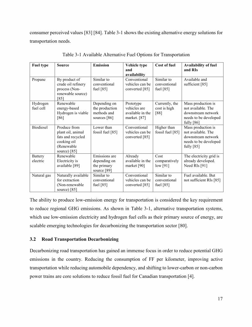
consumer perceived values [83] [84]. Table 3-1 shows the existing alternative energy solutions for

transportation needs.

Table 3-1 Available Alternative Fuel Options for Transportation

Fuel type Source Emission Vehicle type

and

availability

Cost of fuel Availability of fuel

and RIs

Propane By product of

crude oil refinery

process (Non-

renewable source)

[85]

Similar to

conventional

fuel [85]

Conventional

vehicles can be

converted [85]

Similar to

conventional

fuel [85]

Available and

sufficient [85]

Hydrogen

fuel cell

Renewable

energy-based

Hydrogen is viable

[86]

Depending on

the production

methods and

sources [86]

Prototype

vehicles are

available in the

market. [87]

Currently, the

cost is high

[88]

Mass production is

not available. The

downstream network

needs to be developed

fully [86]

Biodiesel Produce from

plant oil, animal

fats and recycled

cooking oil

(Renewable

source) [85]

Lower than

fossil fuel [85]

Conventional

vehicles can be

converted [85]

Higher than

fossil fuel [85]

Mass production is

not available. The

downstream network

needs to be developed

fully [85]

Battery

electric

Renewable

Electricity is

available [89]

Emissions are

depending on

the primary

source [89]

Already

available in the

market [90]

Cost

comparatively

low [91]

The electricity grid is

already developed.

Need RIs [91]

Natural gas Naturally available

for extraction

(Non-renewable

source) [85]

Similar to

conventional

fuel [85]

Conventional

vehicles can be

converted [85]

Similar to

conventional

fuel [85]

Fuel available. But

not sufficient RIs [85]

The ability to produce low-emission energy for transportation is considered the key requirement

to reduce regional GHG emissions. As shown in Table 3-1, alternative transportation systems,

which use low-emission electricity and hydrogen fuel cells as their primary source of energy, are

scalable emerging technologies for decarbonizing the transportation sector [80].

3.2 Road Transportation Decarbonizing

Decarbonizing road transportation has gained an immense focus in order to reduce potential GHG

emissions in the country. Reducing the consumption of FF per kilometer, improving active

transportation while reducing automobile dependency, and shifting to lower-carbon or non-carbon

power trains are core solutions to reduce fossil fuel for Canadian transportation [4].

18

Magnusson et al. emphasized that GHG emissions can be decreased by reducing the consumption

of fuel per kilometers (fuel-efficient vehicles), reducing car use (improving active transportation

and reducing automobile dependency), and shifting to lower-carbon or non-carbon fuels or power

trains such as Hydrogen Fuel Cell Vehicles (HFCVs) and EVs [4]. Hence, vehicle fuel efficiency

improvements in conventional vehicles were considered a prevalent marketing tool by vehicle

manufacturers and marketers in the recent past. However, despite the enhancement of fuel

efficiencies and the affordability of fossil fuels, there has been no decrease in energy consumption

as a whole or in potential GHG emissions, due to high population growth and an increase of vehicle

dependency [92]. Thus, vehicle fuel efficiency improvements have not been affected by transport

energy savings and emission reductions as significantly as expected by decision-makers.

Therefore, past and current researchers and vehicle manufacturers have focused more on

alternative fuel-based vehicles with low- and zero-carbon emissions [80]. Hydrogen fuel cell

(HFC) and low-emission electricity can be identified as the most desirable environmentally-

friendly fuel sources for road transportation [82]. These fuel technologies have their unique values,

and the popularity of these fuels depends on the fulfillment of consumer perceived values [83]

[84]. Table 3-2 shows a comparison of the aforementioned alternative energy solutions considering

their primary energy source, emissions, vehicle type and availability, fuel cost and supply chain

network, and availability.

19

Table 3-2 Comparison of Electric and Hydrogen based transportation with conventional Gasoline transportation

Fuel type Gasoline Hydrogen Electric

Vehicle Types Conventional Internal Combustion

Engine Vehicle (ICEV) [81]

Hydrogen Fuel Cell vehicle (HFCV) [87] Plug-in hybrid electric vehicle (PHEV) & Plug-in

electric vehicle (PEV) [89]

Fuel production

method

Crude oil refining process [80] Alkaline water electrolysis using electricity,

Central steam methane reformation, Central

coal gasification, Biomass gasification and

Thermochemical water splitting with nuclear

Cu–Cl cycle are used to produce Hydrogen fuel

[93], [94].

Hydropower, natural gas-fuelled thermal plants,

biomass power plants, wind power plants, diesel

electricity, solar photovoltaic (PV) energy, tidal

power arrays and geothermal power plants are

used to generate electricity [95]

Fuel

Transportation

Transport through dedicated pipe-lines

over long-distance and distribution using

rail, ship or road tankers [81]

Gaseous hydrogen can be distributed using

dedicated pipe-lines over long distance and the

liquefied hydrogen can be transported by rail,

ship or road tankers [93].

Transport using a smart grid or on-site

production and storage using a stationary battery

pack [96]

Fuel retailing

and re-fuelling

infrastructure

Well established re-fuelling network,

which includes short-term, and long-term

storage facilities, transportation trough

road tankers, ships and pipelines, Oil

separation using refineries and retailing

using fuel dispensers [97].

Gaseous hydrogen can be distributed using

dedicated pipe-lines over long distance and the

liquefied hydrogen can be transported by rail,

ship or road tankers [93]. Dedicated fuel

dispensers are using to re-fuelling the HFCVs.

The infrastructure network needs to be

developed from scratch, which needs extensive

investments.

Grid electricity, Solar or wind electricity retail

through,

Conventional options,

1. Domestic: Level 01 charging [89] [98]

2. Office/commercial: Level 02 charging [89] [98]

3. Public: Level 03 fast-charging [89] [98]

Advanced options:

1. Battery swapping method [99]

2. In-motion/ inductive re-charging [90], [98],

[100].

Fuel-cycle

emissions (W2P

cycle)

Depending on the crude oil extraction,

transportation, and the time of the year

[101] [102] [103]. The average emission

level has been identified as 0.295

kgCO2e per liter of gasoline [104].

Depending on the source characteristics and the

emissions of production, supply, and storage of

the produced hydrogen [86]. Appendix A1

shows the emissions for different production

methods.

The emissions due to electricity production

emissions change with energy source [105]. The

common energy sources and the respective

emission rates are provided in Appendix A2.

20


Vehicle

manufacturing

and emissions

The manufacturing emissions are

assumed as proportionate to the weight of

the vehicle [106]. Based manufacturing

emission for 1532kg weighted vehicle is

2013 kgCO2e [106]

The manufacturing emissions are assumed as

proportionate to the weight of the vehicle [106].

Based manufacturing emission for 1532kg

weighted vehicle is 2013 kgCO2e [106]

The manufacturing emissions are assumed as

proportionate to the weight of the vehicle [106].

Based on manufacturing emission for 1532kg

weighted EV is 2244 kgCO2e including the

battery emissions [106] The average

manufacturing emissions of the EV battery (Li-

ion) has been estimated as 70 kg CO2e per kWh

[107].

Vehicle

operation

mechanism and

emissions

The energy for the conventional vehicle

is generated using gasoline as the fuel

for the Internal Combustion Engine [81].

The operational emission of the vehicles

are depending on vehicle fuel

consumption [108].

It generates electricity inside the HFCV

through an electrochemical reaction of

Hydrogen and Oxygen and operates as an EV

[87]. However, HFCV has on-board fuel

storage, driving range and re-fuelling system as

similar to the ICEV [87]. The vehicle operation

emission can be considered as negligible [108]

The grid electricity or other electricity source is

used to re-charge the on-board battery of the EV.

The battery electricity used to operate the electric

motor of the vehicle [87]. The vehicle operation

emission can be considered as negligible [108].

Vehicle

maintenance

and re-cycling

emissions

End-of-life emissions and emissions

from maintenance and repairs for

automobiles are not significant [35].

End-of-life emissions and emissions from

maintenance and repairs for automobiles are

not significant [35].

End-of-life emissions and emissions from

maintenance and repairs for automobiles are not

significant [35]. The end-of-life emissions of the

EV battery is proportionate to the total mileage

traveled during the vehicle’s lifetime [107].

Approximate

re-fuelling time

and range1

3-5min time for re-fuelling and it has

approximately 500millage per one re-

fuelling cycle

3-5min time for re-fuelling and it has

approximately 500millage per one re-fuelling

cycle [87].

Conventional options: 15min to 8hrs [109]

Advance options: 0min to 2min [110]

Range varies from 110km (Mitsubishi iMiEV)

[111] to 435km (Tesla Model S) [112].

Re-fuelling/

recharging cost

Depending on the proximity to the source

and the time of the year [101] [102]. The

provincial-level average prices of

Due to the cost of the infrastructure and small-

scale production, the average retail price of

Hydrogen is CAD13/kg H2 [88].

The provincial-level average domestic rates of

grid electricity are shown in Appendix A3.

1 Range is known as the estimated driving distance (kilometers) on fully charged battery or full tank of liquid fuel (hydrogen or gasoline) [108]

21


Gasoline for June 2017 are shown in

Appendix A4 [113].

Advantages in

mass-market

adoption

Very convenient to store vehicle on-

board energy

Already experienced by the market and

proven as reliable and affordable [97]

Availability of specialized and extensive

logistics infrastructure network [97]

Very convenient to store vehicle on-board

energy [114]

Vehicle cost can be reduced than EV in mass

production

Decentralized and centralized production is

possible [115]

The infrastructure investment is relatively

smaller than hydrogen due to the use of existing

smart grid [116]

Home-based re-charging stations are available

which may convenient for users [116]

Renewable small scale energy production can be

used to fuel transportation [116]

The

disadvantage in

mass-market

adoption

High GHG emission [92]

High carcinogenic and non-carcinogenic

chemical emissions [92]

High investments in hydrogen infrastructure

and supply chain development

lack of technical know-how [117]

Cost of vehicle-related issues [11], [12]

Range anxiety2 [12], [23]

2 The vehicle range can be varied with on-board energy storage capacity [140], consumption rate and the availability of infrastructure [12], [140]. For widespread

adoption of AFVs, the range can be considered as a physiological barrier [12]. Limitations in available locations of alternative fuel infrastructure and the lower

range of vehicle cause a psychological effect on consumers which is known as “range anxiety” [12], [23]. Range anxiety makes potential consumers to decide

against the use of AFVs [21]–[23].

22

Hydrogen is the least capable technology to take advantage of the existing or low-cost fuel

infrastructure investment where the hydrogen fuel infrastructure investment is significantly higher

than the electricity fuel infrastructure cost [116]. Therefore, the electricity-based transport system

is preferred for this study3. Alternative fuel-based transportation can be compared and evaluated

with the viability of alternative fuel vehicles by explaining the life cycle based emission and cost

of each vehicle and fuel cycle [118].

3.3 Transportation Electrification

Transport electrification consists of energy and mobility sectors [119]. The energy sector consists

of energy generation to energy storage and distribution system (e.g. smart grid for electricity),

whereas the mobility sector consists of using alternative fuel-based vehicles (e.g. EVs and HFCVs)

for transportation [119].

Energy Sector: Regional electricity emissions and costs vary with the grid electricity mix and the

primary energy source. The electricity grid energy mix, costs, and overall emissions for Canada

are shown in Appendix A3. Moreover, the recharging of EVs from the existing electricity grid may

result in higher electricity demand [89]. The current electricity transmission system is optimized

for the current electricity usage, and additional electricity consumption may destabilize the system

[96]. This may cause high overloads in the on-line transformers, feeder congestion, and undue

circuit failures [120][121]. Therefore, it is essential to consider the “feeder capacity” (electricity

supply or excess electricity availability) when allocating recharging infrastructure for EVs.

Mobility Sector: The “time required for recharging,” “access to the recharging infrastructure,”

and “government policies” are the critical concerns in an EV recharging infrastructure network.

Additionally, having “home charging access” has been identified as the most significant predictor

for future PEV interest [10]. People living in apartments or condos do not have access to their own

recharging stations [122], so a properly arranged public charging (Level 3) network will be

3 A regional based analysis was done using literature-based data to evaluate the different energy options for British Columbia (BC) transportation

needs. Accordingly, Electricity-based transportation was identified as best clean energy technology for BC. "Are we ready for alternative fuel transportation systems in Canada: A Regional Vignette” Submitted to Journal of Cleaner Production (Elsevier) in February 2017. (Menu script:

JCLEPRO-D-17-00819)

23

beneficial for a widespread increase in EVs. The geographical, economic, and environmental

constraints are considered the core concerns for the spatial planning of EV-RIs [15]. Land-use

patterns such as potential developments, traffic generation, and distribution, etc. can be integrated

into the transport infrastructure plan by linking national political and social conditions, such as

government policies and consumer behaviours [15].

Generally, the energy sector and mobility sector are connected via an optimal network of electric

vehicle recharging infrastructure.

3.4 Recharging Infrastructure for Electric Vehicles

“Level 1 (Domestic),” “Level 2 (Domestic and Work),” and “Level 3 (Commercial or Public)” are

the conventional plug-in recharging infrastructure (RI) types currently available for day-to-day use

in electric vehicle recharging [89]. In addition, extensive research is being conducted on enhancing

re-charging speed while reducing system losses. Current research is focusing on: 1) Innovative

ways to enhance battery storage capacities; 2) Innovative ways to implement in-motion charging

mechanisms, which will reduce initial vehicle cost and allow travel with higher mileage [123]; and

3) Innovative ways to establish net-zero energy systems using renewable distributed energy

systems. Currently, the following recharging infrastructures and techniques are found in the

literature:

1) Level 1 chargers are developed for household use using domestic electricity (110-120V)

[89][98]. This is the cheapest recharging infrastructure investment [98], with a cost of around CAD

150 - 500 for basic installation [98]. The charging time is comparatively high (11-36 hours) [98]

and the cost of re-charging is comparatively low [87].

2) Level 2 charging is done using 220-240V charging points [98][10]. This is an additional

installation for potential PEV consumers, at a cost of CAD 1,600 to CAD 12,000 depending on

labour charges [87][89]. The charging time is 2-6 hours, depending on the vehicle battery capacity

[98].

3) A Level 3 type charging station uses 208–600V electricity and offers fast, direct-current

recharging (DC-FC). It has high voltage output and charging is done within 0.4–1 hour based on

24

the EV battery capacity [89][98]. This facility would cost around CAD 35,000 to CAD 46,000

[87]. Level 3 type is used for public recharging facilities for consumers who prefer high-speed

charging [98].

4) The battery-swapping infrastructure is another innovative and proven EV recharging concept.

In this system, the EV battery is owned by the company that operates the battery swapping facility

[13][124][99], so the battery and the electric vehicle are considered two separate cost and

ownership entities [13]. Battery swapping infrastructure-based systems will potentially reduce EV

battery replacement cost (due to the battery being owned by the company) [99] and vehicle capital

cost (upfront vehicle cost without battery) [13][99], and increase the vehicle’s driving range [99].

5) Additionally, current research studies are focusing on EV in-motion charging by wireless power

transmission technology using the inductive power transfer concept [98][100][90]. In such a

system, EV designers can use low capacity batteries, which reduces the battery purchase cost and

thereby reduces the purchasing cost of the EV [90]. Moreover, in-motion charging can be used to

reduce the constraints related to energy storage and existing charging issues [98][90], and mitigate

the charging time obstacles and range related issues [125] by providing a significant amount of

energy on the roadway. However, high capital investment is required to modify existing roadways

for wireless power transfer technology [110].

The use of the above recharging facilities and potential investments vary with several factors

related to consumers, investors, and developers. Consumer behavioural factors, consumer cost

perception, consumer concerns about energy depletion and GHG emission, range expectancy, and

current and potential incentives and taxes are critical factors in deciding to switch to EVs. Those

factors are further discussed below,

3.4.1 Incentives and Policies to Encourage EVs and EV-RI Investments

Several countries provide incentives to encourage the use of cleaner vehicles to reduce potential

GHG emissions. The government contribution in the top four countries, Norway, the Netherlands,

China, and the USA, is discussed in Table 3-3 to identify favourable potential government

incentives for Canada.

25

Table 3-3 Potential Incentive for Electric Vehicles

Region/

Country

Capital incentives Operational incentives Disposal

incentives

Ref.

Norway Exempt purchasing tax and

25% value-added tax

Reduce 50% of tax if an EV

is used as a company vehicle

Exempt from annual vehicle tax

Exempt road tolls

Free parking at Municipal parking facilities

Access to transit lanes

Exempt from car ferry charges

None [126]

[127]

Netherlands Reduce purchase tax

Purchase rewards to

commercial EVs

Conventional vehicle scrap

reward for potential EV

buyers

Exempt monthly road tax

4% taxable income additions for EV drivers

Environment investment allowance up to

36%

On-the-road-electric mobility

Free EV parking facility

Subsidiary for EV home recharging

None [128]

[127]

Shanghai,

China

Government subsidies for

EV purchases

Exempt from license plate

lottery system

Exempt from road tolls

US$14 billion for EV recharging

infrastructure development

Exempt

from sales

tax

[127]

California,

USA

Federal and local

government income tax

credit for EV users

Rebates to switch from

conventional vehicle to EVs

Reduce register and license

plate tax for new purchases

Access to HOV lanes

PEV only parking space

Motor vehicle inspection exemption and

emissions testing waiver

Toll reduction and exemptions

EV infrastructure tax exemption

EV battery tax exemption

Exemption from state fuel taxes

Free recharging at state-owned charging

facilities

Sales tax

reduction

[129]

Although these policies have significant positive outcomes (see Table 3-3) that contribute to the

development of clean energy-based transportation, there can be adverse impacts on the

government. As an example, income from toll fees, parking fees, and ferry fees will not be

sufficient for future infrastructure investments and regular maintenance of the existing

infrastructure [128]. However, Transport Canada is currently working on EV-favourable policies

for Canadian transportation, and the province of BC has allocated CAD 40Mn to improve its EV

infrastructure and related policies [62][63].

Although government and government-related institutions provide incentives for both energy-

efficient buildings and vehicles, household transportation and residential buildings are considered

separate entities in planning incentive schemes. Hence, incentives for households have been

introduced on an ad-hoc basis, ignoring the integrating effect of energy consumption for household

transportation and domestic activities. Therefore, it is vital to introduce a comprehensive model to

26

integrate residential economic activities and their resulting emissions with the resulting emissions

of vehicle-based economic activities. A comprehensive literature review revealed that there is a

lack of knowledge of incentive planning for overall household energy reduction [130]. Evaluation

and selection of the optimal incentive out of the feasible options is a formidable task that needs a

scientific platform. Even though the literature is saturated with multi-criteria based retrofit

selection tools for buildings [44][45][46], there are no comprehensive frameworks to select overall

household energy interventions that suit the expectations of multiple stakeholders. A proper energy

intervention selection framework would be used to identify an integrated set of government

policies and practices that guide consumers to a low-emission based economy [70]. National,

provincial, and municipal governments and non-government institutions are more concerned with

local emission trends related to residential buildings and transport, as they need to reduce their

GHG emissions and achieve their GHG targets quickly.

3.4.2 Consumer Recharging Behaviours

Per the Canadian survey on transport electrification, about 63% of EV users rely on overnight

charging at home, and having home-based charging access is identified as the most significant

predictor for EV interests in the future [10]. However, consumers who recharge using public

recharging facilities tend to refuel in pre-defined areas according to their mental maps and are

usually refueling at the beginning or end of their journey [131][132]. In this case, the refueling

station is known as the “brick & motor” location [84] and the business is driven by the destination

or the location [84]. In simple terms, the re-fueling facility needs the physical presence of the

consumer/vehicle in order to fuel the vehicle [84]. The main disadvantage of plug-in re-charging

facilities is the safety concerns in a wet and hostile environment, longer access to the recharging

units, and extensive time needed for recharging [90][109][123].

3.4.3 Consumer Concerns about Energy Depletion and GHG Emissions

Although Canadian transportation sectors contribute more to the national GHG inventory, the

literature reveals that the consumer perception of energy on emissions in the Canadian residential

sector is significantly higher than the transport sector. Canadian households contribute to GHG

emissions directly and indirectly. Direct emissions are comprised of emissions from residential

27

energy use and emissions from motor vehicle use, while indirect emissions are GHGs emitted

when producing goods and services for household use [133]. In 2015, the residential sector

consumed about 17% of domestic energy and contributed to 14% of the national GHG inventory

[134]. Household energy consumption and GHG emissions depend on factors associated with

building type, envelope characteristics, household transport mode, and consumer behaviours [39].

Some research is focusing on studies related to building energy retrofits, and other research is

focusing on interventions for transportation-based GHG reduction. According to the literature,

numerous studies have been conducted to identify potential building energy retrofits to reduce

energy consumption and emissions of residential buildings [40][41][42][43]. Gustafsson et al.

(1991), Flourentzou et al. (2002), and Asadi et al. (2012) developed models to optimize building

energy consumption, thermal comfort, and retrofit costs [44][45][46]. The use of a life cycle

assessment-based approach to identify optimal retrofits for net-zero emission buildings has been

conducted by Ruparathna et al. (2017) [47]. In contrast, energy-efficient transport interventions

were identified to reduce transport-based GHG emissions [48][10]. However, there is a lack of

knowledge on the combined research approach, which considers both building energy retrofits and

low-emission transport interventions considering household consumer behaviours, local utility

emissions, costs, etc.

3.4.4 Consumer Cost Perception

Per the transport survey done by Canada and Norway, the cost of fuel factors heavily in current

EV users’ decision to buy an electric vehicle [24][10]. In the Norwegian market, 41% of consumers

buy EVs to save money [24], whereas the Canadian survey showed that the Canadian EV market

is also sensitive to vehicle operating cost, which is mainly the price of fuel [10]. However, the

study done by Turrentine et al. suggested that, practically, automobile owners do not have basic

costing attributes to make calculated decisions on better fuel economy, and most of them do not

track their fuel cost over a significant period [135]. The fuel cost for EV depends on local

electricity prices [136]. Accordingly, the fuel cost of EVs can be considered CAD 3 per 100km to

CAD 4 per 100km in BC, depending on the vehicle type for domestic charging facility. The cost

of public recharging, however, varies with costing policy; some charge CAD 0 to 10 per hour [91]

while others charge it as a parking cost [91].

28

Moreover, the life cycle cost of the battery is the main component of the EV life cycle cost [137].

This includes the purchasing cost of the battery, battery lifetime, battery cycle time, battery

replacement cost, etc. [137]. High costs of batteries will increase the switching costs and user costs

of EVs as well as increasing the insurance and registration costs of the vehicle [137].

3.4.5 Range Preference of Vehicle Consumers

“Range” can be described as the mileage expected by the consumer in a single refueling cycle [12].

EVs have been designed with an inadequate battery level, which makes it impossible to travel

longer distances in one charging cycle due to the high cost of high capacity batteries [21][22][80].

Tran et al. (2013) suggested that increasing recharging facilities may offset the consumer

expectation for a long-range vehicle [138][139]. Limitations in the available locations of EV-RI

and the lower range of vehicles cause a psychological effect on consumers, which is known as

“range anxiety” [12][23]. Range anxiety makes potential consumers decide against the use of EVs

[21][22][23], so the limited range of affordable EVs and limited EV-RI facilities are considered

critical constraints for the widespread adoption of EVs [12]. This barrier can be mitigated by

scientifically improving charging opportunities to enhance them at minimal cost. Having said that,

there are only a limited number of EV recharging facilities in Canada compared to traditional

(gasoline) refueling facilities due to the lack of EV demand [23][140][141]. Therefore, an efficient

EV-RI network (EV-RI system) is vital for widespread adoption of an EV-based transportation

system in Canada.

3.5 Planning Electric Vehicle Recharging Infrastructure

Infrastructure system planning plays a vital role in transport system planning [142]. The approach

used for this can vary with infrastructure use and characteristics such as type, capacity, location,

etc., source characteristics, economic factors, consumer demands, government policies, and

procedures [143].

Generally, macroscopic modeling is used for system planning. According to Pollalis (2016),

sustainable infrastructure system planning can be explained using a four-level approach [20]:

29

1. Determine the demand and consumption required to service by the proposed infrastructure

system.

2. Develop a strategic approach to employ resources to achieve the required demands.

3. Identify facilities and operations that realize the strategic plans developed.

4. Locate facilities and operations to cover the spatial needs of the system.

Accordingly, the travel demand assessment and facility location-allocation are critical elements in

infrastructure system planning.

3.5.1 EV Demand Modeling and Sustaining Approaches

Travel demand forecasting and sustaining the current and potential demands are vital to ensure the

continuity of EV-based transportation systems. In these cases, travel demand forecasting models

are used to evaluate the impacts of land use, transport facilities, infrastructure, and demographic

changes in the existing transport system [144]. Firstly, existing transportation systems need to be

decoded to estimate transport demands in the future. The transport system decoding model

includes four-steps: trip generation, trip distribution, mode split modeling, and trip assignment

[20]. Secondly, behavioural models can be used to investigate the impacts of incentives and taxes

that can be used to sustain EV demands through variations. Thus, EV-RI locations can be

strategically assigned, considering anticipated EV demands.

3.5.1.1 Estimate and forecast EV demands

Estimated and forecasted trips can be estimated using trip generation models that can be developed

initially. The purpose of trip generation is to understand the need for transportation. Trip (𝑇𝑖𝑗𝑘𝑛)

can be described as a one-way movement from origin to destination, which can be classified as

home-based (THB) and non-home-based (TNHB) trips [145]. Trip generation models are used to

describe trip lengths, distribution in time, the number of trips generated, trip classification, and

land-use pattern (trip generation and attraction) [20]. Generally, the trip pattern changes with

socio-demographic and land-use factors [145]. The theory of adoption and diffusion (Rogers

diffusion model) [146], explains the market growth of an innovative product, which can be applied

to EVs as well [34]. Accordingly, EV consumers can be categorized as innovators, early adopters,

30

early majority, late majority, and laggards [50]. Table 3-4 shows the typical EV technology adopter

categories and their behaviours.

Table 3-4 Maturity Stages of the EV Market and Consumer Behaviours [50]

EV consumer type Description

Innovators Technologically savvy, high-risk appetite, high-income category

Early adoptors Younger in age, high income, highly educated, Socially forward, high opinion leadership

Early majority Slow adoption, average social status, imitators, average opinion leadership

Late majority Average income, low social status, high imitators, low-average opinion leadership

Laggards No-opinion leadership, No risk appetite, “traditional” behaviours, generally “business-

as-usual” type

According to the expectation of the above consumer categories, trip behaviour can be changed

with the dynamic EV market. Therefore, the trip classification needs to be defined according to

the expectations of the actual users [50]. Linear regression modeling and cross-classification

modeling are conventional techniques used for trip generation simulations [145]. However, these

models have extensive data requirements, which are based on travel surveys of the considered

traffic zones.

Moreover, trip distribution modeling can be used to match the origins and destinations (O-D) of

the trip generated and develop a “most-likely” trip matrix considering multiple zones. A gravity

model can be used to define the trip matrix (O-D matrix) for a given network, which is given as

Equation (1).

𝑇𝑖𝑗 = 𝛼 𝑂𝑖𝐷𝑗𝑓𝑖𝑗 Equation 1

Where, α – proportionality factor, 𝑓𝑖𝑗 − The generalized function of time, distance, and cost [144]

Generally, forecasting of continuing patterns and/or relationships are easy to model, while pattern

changes are complicated to model [147].

31

3.5.1.2 Extended EV demands using EV favourable cost and incentive policies

Developing the mode-choice model will support examination of social, economic, and

environmental impacts to society from the proposed modes [20]. Multinomial Logit Model is the

conventional method to achieve mode-choices of trip makers. Axen et al. (2015) used the

Multinomial Logit Model to develop an EV market share assessment model for BC [34]. A survey

approach was used to obtain the data required to train the developed model, which included a

survey sample of 538 respondents in BC [34]. The Norwegian and Californian policies were

considered the best global regulatory due to the highest EV per capita globally. Hence, Norwegian

and Californian EV-favourable policies4 were considered strong demand-focused policies [34].

Literature reveals that the availability of multiple charging point access and the cost of electricity

are the key supply-based factors, which could affect the selection of EVs by a potential vehicle

buyer.

3.5.2 Facility Location Selection

The facility location selection can be “Macroscopic (macro-level)” and “Microscopic (micro /

individual-level)”. The macro-level can be defined as regional or community level RI network

planning, whereas the micro-level is individual level facility planning. The UBC TIPS lab shows

a scenario-based approach to identify individual sites for EV-RI locations [50]. Visibility,

convenience, cultural branding, reliability, affordability, operating cost, initial cost,

competitiveness, gas vehicle displacement, and energy use were used as multiple attributes to rank

the alternative locations for each scenario [50]. However, the macro-level planning approach has

not been considered in this study.

As a macro level, long-range planning mechanism, RI locations need to be placed strategically by

considering the locations of neighbouring facilities that cater to the dynamic demands of EVs in

the future. An optimization approach can be used with a multi-period demand assessment. A

content analysis was conducted for Automated Teller Machines (ATMs), gasoline stations,

4 Refer to Table 3-3 for Norwegian and California EV favourable policies.

32

convenience stores, and EV recharging station location-allocation research-based publications.

Multi-objective genetic programming and particle sworn optimization were identified as the

standard mechanisms used to simulate the aforementioned models [148][149]. Table 3-5 shows

the published literature on transportation-based location optimization.

Table 3-5 Existing Solutions for Optimal Infrastructure Location-Allocation

Author/s Model developed

Objective

function

Constraints and

parameters used Approach

Methods

Used

Ref

No.

Ma

xim

ize f

low

ca

ptu

red

Min

imiz

e c

ost

Ra

nge

Wa

itin

g/a

cce

ss

tim

e B

att

ery c

ha

rgin

g

eff

icie

ncy

/tim

e

Gri

d c

on

strain

ts

By

-la

w c

on

strain

ts

Sin

gle

sta

tio

n

ba

sed

C

orri

dor b

ase

d

Netw

ork

-ba

sed

Kuby and

Lim

(2005)

The flow-refueling location

problem for alternative-fuel

vehicles

√ √ √ MIP [35]

Upchurch,

Kuby, and

Lim,

(2009)

Capacitated flow refueling

location model (CFRLM)

based on flow capturing

location model (FCLM)

√ √ √ √ MIP [26]

Lim and

Kuby

(2010)

Heuristic algorithms for

siting alternative refueling

location using FCLM

√ √ √ MIP [27]

Kim and

Kuby

(2012)

The deviation-flow

refueling location model

(DFRLM)

√ √ √ MILP [150]

Capar and

Kuby

(2012)

An efficient flow refueling

location model for

alternative-fuel stations

√ √ √ MBIP [151]

Chen,

Kockelma

n, Khan,

(2013)

EV charging station location

problem: parking based

assignment method to

Seattle

√ √ √ √ MIP [28]

Shao-yun,

Liang,

Hong, and

Long

(2012)

The planning of EV

charging stations in the

urban area (location and

sizing)

√ √ √ √ √ Queuing

theory

[37]

Mehar and

Senouci

(2013)

An optimization location

scheme for electric charging

stations

√ √ √ GA [152]

Yan

(2014)

Optimal layout and scale of

charging stations for EVs

√ √ √ √ Heuristic

algorithm

[36]

Huang et

al. (2010)

A GIS-based framework for

bus network optimization

√ √ √ GA and

GIS

[29]

Wang and

Lin (2013)

Locating capacited multiple

types of recharging stations

√ √ √ √ √ √ MIP [30]

33

Grid constraints such as substation capacity, charging power, node voltage aptitudes, feeder mix,

and access point capacity are the key constraints related to the electricity grid [152]. The

constraints stated on government policies, by-laws, and guidelines need to be assessed in order to

ensure a standardized EV recharging infrastructure network [26]. Moreover, either “cost

minimization” [152][37] or “flow captured maximization” [35][26] were selected as an objective

for the above methods. According to Table 3-5, mixed integer programming (MIP) and genetic

algorithms (GA) are the most common techniques used to solve this problem. However, Wang and

Lin (2013) developed a method using mixed-integer programming by considering both “cost

minimization” and “flow captured maximization” to locate slow-recharging stations [30].

Moreover, Li et al. (2009) studied the teller machine location optimization problem where the

“return on investments maximizing” was considered an objective function to maximize the returns

on investment [149]. Hence, they expect to ensure the maximum returns from those machines for

a sustainable service.

Geographic information systems (GIS) can be used as a spatial analytical tool in this study [29]

[149]. The main purpose of the GIS platform is to convert the continuous plan into a coordinate

grid system [153]. According to the study done by Liu et al. (2006), mixed integer programming

and genetic algorithms can be coded using C, C++, and PYTHON. These scripts can be registered

into a dynamic link library [153]. Those coded functions can be linked to the macro Visual Basic

script in ArcGIS that can be called upon to proceed with the optimization [153].

3.5.3 EV-RI Construction, Maintenance and Disposal Process

Infrastructure systems are subjected to construction, maintenance, and rehabilitation [154].

Effective management of infrastructure leads to maximized benefits to all stakeholders [154].

Generally, risk factors such as political risk, construction risk, legal risk, economic risk, operation

risk, market risk, project selection risk, relationship risk, project finance risk, and inherent risks

are significant in infrastructure development and maintenance projects [155]. The project time,

costs, and quality performances of a construction project will be affected by the risk involved

[156].

34

According to 3.4.1, EV demands are increasing with government regulations, which leads to an

increase in recharging demands. The capacity of EV-RIs needs to be increased with time to ensure

maximum access for potential EV consumers. However, these EV demands have significant

uncertainty on RI development scope and financials. Hence, the financial risk (due to EV demand

uncertainty) and scope changes (due to capacity required) are critical factors for the

implementation of EV-RI facilities.

3.5.4 Project Delivery Methods

A project delivery method (PDM) is a method of procurement in which the project risk and

performance can be transferred to other parties [54]. This can be used to establish a framework for

the design, procurement, and construction of infrastructure projects. The selection of an

appropriate PDM is one of the core decision strategies that affect the successful completion of a

project [157]. This will drive project cost, quality, and schedule [158]. Generally, PDMs can be

categorized as traditional, collaborative, integrative, and partnership strategies [159]. Sample

PDMs in these four categories, which are commonly used in the construction industry are listed in

Table 3-6.

The selection of an appropriate PDM is vital to ensure successful project completion [157].

Conventionally, the choice of the PDM is made as part of the procurement strategy. In most cases,

this decision is made by the owner with the help of the project manager at the project pre-planning

stage [160]. In general, a PDM evaluation matrix is prepared by the project manager, and the owner

selects the PDM method based on the details given in the matrix [161]. The factors considered in

these matrices vary with the project and the expertise of the project managers. Mafakheri et al.

(2007) have shown that the project delivery method is based on the project cost, schedule, quality,

complexity, value engineering, experience, risk, scope changes, uniqueness, external approvals,

culture, financial guarantee, and project size [162]. A study, done by Vanhouche (2012) identified

that project complexity (technical know-how), project risk, and project are critical factors in PDM

selection [163]. Moreover, the Government of Idaho proposed that complexity and innovation,

delivery schedule, level of design, risk, agency factors, market factors, and third party coordination

are critical factors in selecting an appropriate PDM for a dynamic project [161]. However, there is

very little scientific knowledge of PDM selection using MCDM.

35

Table 3-6 Literature-based Typical Project Delivery Methods

PDMs /

Category

Description Advantages Disadvantages Ref

Design-Bid-

Build (DBB)

- Traditional

In DBB, design, and

construction are considered as

separate entities. Construction

starts once the design is

completed. The bidding will

be followed afterward.

Familiar PDM

Defined roles and

responsibilities

Presents the lowest possible

cost to the building

High potential for

change orders and

conflicts

No cost-sharing

No “fast-tracking”

available

[164]

[165]

Design-Build

(DB) -

Collaborative

The private party will be

responsible for designing and

building the total project.

Single contract for design and

build

Can proceed with fast track

projects

No change orders needed

Cost-sharing is possible

The owner has limited

involvement, The

process will not bring

the best design and

best builder together

Quality checks will be

done by the contractor

[164]

[165]

Design-

Build-

Operate-

Transfer

(DBOT) -

Partnership

Public property owner enters

into the contract with a private

party for the design,

construction, finance, and

operation for a pre-authorized

period. Ownership will be

transferred afterward.

An external source of capital

Time-saving (speed-up with

the private sector experiences)

Cost-saving (By using the

private sector contracting

mechanisms)

Risk transferring possible

Lack of familiarity in

similar applications

Specialized projects

Limited public owner

control over the

project until the

transferring is done.

[166]

Build-Own-

Operate-

Transfer

(BOOT) -

Partnership

Public property owner enters

in to contract with a private

party for the design,

construction, finance, and

operation for a pre-authorized

period of time. The ownership

will be transferred to the

public owner at the end of the

period. (used for large scale

projects).

An external source of capital,





mechanisms), Risk

transferring (finance, quality,

schedule, operation, and

maintenance), Possibility to

control over the design

Lack of familiarity in

similar applications

Specialized projects

Change orders might

be possible

[164]

Public-

private

partnership

(PPP) -

Partnership

A corporate venture between

private and public partners to

achieve a common public goal

by using their expertise

through proper resource

allocation, risk-sharing, and

rewarding.

An external source of capital





mechanisms) Risk-sharing is

possible

The conflict between

public sector welfare-

based objectives and

private sector profit-

based objectives

[167]

[168]

[169]

Construction

Management

at-risk -

Collaborative

An owner selects the

construction manager (CM)

based on his qualifications and

fees. Then the CM has to

represent the owner and

proceed with the construction.

Ensure high quality at

minimal cost, owner transfers

the risk to CM, Cost-sharing

is possible CM will be

selected based on

qualifications and fees.

Perceptional price

competition is limited.

The owner has limited

control over general

contractors

[165]

Integrated

Project

Delivery

(IPD)

Collaborative

A collaborative alliance of

project resources (people,

systems, equipment etc.,) to

acquire optimal project

performance. A trust-based

method focuses on the overall

project goal.

Mutual respect and trust,

Scope and goal definition,

risk, cost-sharing are possible,

the project schedule can be

dynamic and project quality

control is better than other

PDMs.

Control over the

design and

involvement after

awarding are limited.

[170]

36

An AHP-based tool was developed to evaluate the above parameters and select the most suitable

project delivery method from prior-selected PDMs [162]. However, in some developments such

as the deployment of EV-RIs, demand uncertainty would lead to significant structural and cost

variations in the optimal refueling infrastructure network [53][71]. Thus, cost and demand

uncertainties need to be captured for selection of the most desirable PDMs for EV-RI deployment

projects. Mostafavi, A. et al. (2010) describe a fuzzy TOPSIS-based approach to incorporate

project uncertainties to select project delivery methods for construction projects [157].

EV-RIs can be considered smaller-scale infrastructure developments than traditional

transportation infrastructures such as roads, bridges, etc. Local developers, investors, and other

decision-makers do not have much knowledge of the deployment at the early stage of EV-RI

deployment projects. Hence, the use of multi-stakeholder synergies will be vital for successful

implementation of EV-RI networks in urban communities. In that case, selecting PDMs

considering the rogers model to evaluate EV recharging market factors and incorporating multiple

stakeholder opinions would enhance project performances [71]. There is a lack of knowledge on

an integrated approach to select PDM strategies based on the owner, project manager and other

relevant stakeholders' opinions for novel and long-term projects similar to EV-RI deployment.

3.6 Environmental and Economic Assessments

The life cycle environmental and economic assessment can be conducted using a life cycle

assessment (LCA) and life cycle cost assessment (LCC) [171]. Accordingly, the LCC and LCA

are explained as follows.

3.6.1 Life Cycle Assessment (LCA)

The life cycle assessment (LCA) is an important process development technique in terms of

environmental sustainability [172][173]. According to the United State Environmental Protection

Agency, LCA can be defined as “A methodology for estimating the environmental burdens of

processes and products (goods and services) during their lifecycle from the cradle to the grave”

(USEPA 1995), and according to the Society of Environmental Toxicology and Chemistry, LCA

is defined as “A process to evaluate the environmental burdens associated with products,

processes, or activities by identifying and quantifying energy and material used and water released

37

to the environment; to assess the impact of this energy, and material uses a release to the

environment, and to identify and evaluate opportunities to affect environmental improvements”

(SETAC 1993).

ISO 14041 shows a comprehensive framework of LCA with the respective phases to be conducted.

According to Figure 3-2, the life cycle assessment consists of a goal, scope, inventory analysis,

impact assessment, and interpretation. The goal of the LCA consists of the objective, the target of

the audience, and the reason for the study [174]. LCA focuses on the environmental impacts of the

process/product over its total life cycle. LCA enables decision-makers to improve the

environmental performance of a particular product in a strategic planning process [118].

The scope of the LCA study consists of the functions of the product system, the functional unit,

the product system boundaries, allocation procedures, types of impact and methodology of impact

assessment, subsequent interpretation to be used, data requirements, assumptions, limitations,

initial data quality requirements, type of critical review if any, and type and format of the report

required for the study [174].

According to ISO 14041, the life cycle inventory analysis and results interpretation include the

following steps. 1) Inventory classification that is required to assign each inventory item to

different impact categories; 2) Life cycle impact identification by converting inventory items into

impacts using conversion factors, which is called characterization; 3) Normalizing potential

impacts into a comparable format; 4) Grouping impacts and assigning weights to emphasize the

importance of each impact category; and 5) Evaluating the life cycle impact assessment results.

Life Cycle Assessment Framework

Goal and Scope

Definition

Inventory Analysis

Definition Impact Assessment

Interpretation

Figure 3-2 LCA Framework as Shown in ISO14041

38

The inventory analysis needs to be conducted after the scope definition in order to identify the

overall life cycle inventory. According to GREET, the vehicle life cycle can be divided into two

key cycles.

Vehicle Life Cycle: The vehicle life cycle study is comprised of vehicle manufacturing, vehicle

operations, and vehicle end-of-life [175][176]. Vehicle life cycle (LCA_V) emissions can be

explained as Equation (2) as follows:

LCA_V = E + Erecurring + Eend-of-life Equation 2

Where, E – Vehicle manufacturing emissions (kgCO2e), Erecurring – fuel-based operational

emissions and maintenance emissions (kgCO2e), Eend-of-life – End-of-life emissions (kgCO2e)

Fuel life cycle: Fuel life cycle can be categorized as “Well to Pump cycle (W2P)” and “Well to

Wheel cycle (W2W)” [177]. The feedstock (including feedstock recovery, transportation, and

storage) and fuel (including fuel production, transportation, storage, and distribution) are

cumulatively known as the W2P cycle [177]. The extended cycle, which includes the operational

phase emissions of the vehicle, is known as the W2W cycle [177]. Both of these processes generate

emissions and consume energy. According to Argonne National Laboratory (2016), the

relationship between the vehicle cycle and the fuel cycle can be shown in Figure 3-3.

Raw Material Extraction

Vehicle

Manufacturing

Vehicle

Operation

Vehicle

Maintenance/

Repair

Vehicle Disposal

Vehicle Life

CycleFuel Life

Cycle

Fuel Production /

Electricity

generation

Transportation /

Transmission

Retailling

Raw Material

Energy

Environmental

Impacts

Economic

Impacts

Figure 3-3 Conventional Vehicle Life Cycle and Fuel Life Cycle [8]

39

3.6.2 Life Cycle Cost (LCC)

Life cycle cost (LCC) can be defined as the external and internal costs associated with a project or

a process over its total lifetime [178]. The LCC can be assessed for the life cycles of fuel and

vehicle to obtain the complete life cycle of vehicle transportation. As described in section 2.1, the

vehicle purchase/manufacturing cost, operational cost, maintenance cost, repair cost, recycle cost,

fuel extraction, storage, transportation, and retailing cost are major parts of the vehicle life cycle.

The LCC for a product can be expressed as Equation (3) [179].

LCC = C + PV recurring – PV residual-value Equation 3

Where, PV recurring = Present value of the all recurring costs, C = Initial investment / purchase cost,

PV residual-value = Present value of the end-of-life value

NPV and annualized cost can be calculated by using Equation (4) and Equation (5) [180],

𝑁𝑃𝑉(𝑖, 𝑁) = ∑𝑅𝑡

(1+𝑖)𝑡𝑁𝑡=0 Equation 4

𝐸𝑞𝑢𝑖𝑣𝑎𝑙𝑎𝑛𝑡 𝐴𝑛𝑛𝑢𝑎𝑙 𝐶𝑜𝑠𝑡 = 𝑁𝑃𝑉 . (𝑖

1−1

(1+𝑖)𝑡

) Equation 5

Where: NPV -Net Present Value, Rt - net cash flow, i - discount rate, N - study period, t - time of

the cash flow

Vehicle fuel cost depends on energy production costs, supply chain cost, and retailer overheads.

The energy production costs vary based on the energy source and the production method.

Moreover, alternative fuel infrastructure cost varies with respect to the refueling infrastructure

capacity [87], refueling/recharging method [181], safety requirement [181], service radius [181],

terrain condition [181], and environment conditions [181]. Reducing the cost of alternative fuel

sources is the core factor in motivating users to shift from traditional transportation to alternative

energy transportation [24][10][182]. Therefore, the alternative fuel infrastructure costs need to be

kept to the minimum, in order to provide low-cost fuel [177][181].

40

3.6.3 Eco-efficiency Assessment

Eco-efficiency is a concept that is used to measure the combined effect of environmental and

economic costs and benefits of a particular product or product system through its entire life cycle

[183]. Huppes and Ishikawa (2007) described a concept called “eco-efficiency ratio” to compare

different alternatives and to identify trade-offs in order to select the best alternative [184]. Using

general terms, the units of value generation per unit of environmental impact is known as the eco-

efficiency of the particular product [183][185]. Equation (6) can be used to calculate the eco-

efficiency ratio.

Eco − efficiency Ratio = Value generation ($)

Units of enviornmental impacts (kg CO2eq) Equation 6

3.7 Multi-criteria Decision Making

Multi-criteria decision making (MCDM) is prevalent in engineering applications, where the

decisions are related to complex problems with conflicting objectives and multiple stakeholders

[186]. MCDM problems are described using a decision matrix to indicate multiple attributes and

alternatives [187]. These methods can be categorized into non-compensatory and compensatory

methods based on the decision-making approach.

Non-compensatory methods: These methods can not be used for decisions where there are no

trade-offs between multiple attributes [187]. In this case, each attribute stands on its own, and the

comparison should be made based on the individual attribute [187]. Dominance, maximin,

maximax, conjunctive-constraint, and disjunctive-constrain are some of the common non-

compensatory methods used for engineering applications [187].

Compensatory methods: These methods are used to incorporate trade-offs between multiple

attributes during the decision-making process [187]. The following compensatory methods are

frequently used for engineering applications.

1) Scoring methods – Here, a score is used to express the decision-makers’ preference for each

alternative [187]. Analytical Hierarchy Process (AHP) and Simple Additive Weighting method are

popular scoring methods used in the literature.

41

2) Compromising methods – These methods choose the best desirable alternative that has the

lowest distance to the ideal solution [187]. The Technique for Order Preference by Similarity to

Ideal Solution (TOPSIS) method is a prevalent compromising method for engineering

applications.

3) Concordance methods – These methods establish concordance measures and generate a

preference ranking to obtain the best desirable solution [187]. In this case, alternatives with highly

ranked attributes should get higher ranks. The linear programming method is a prevalent approach

that uses concordance-based decision-making.

4) Evidential Reasoning Approach – This is a novel MCDM approach in which each attribute of

an alternative is denoted by a distributed assessment using a belief structure [187].

The above-mentioned MCDM methods can be used to obtain ideal solutions, non-dominated

solutions, satisfying solutions, and preferred solutions based on the nature of the problem, nature

of the desired solution, and the method used. Moreover, these methods can be further improved by

integrating uncertainty.

3.8 Decision-making under Uncertainty

Uncertainty can be described as the vagueness of available data and lack of data availability.

Several methods can be used for decision making by incorporating the data and project

uncertainties, where the Scenario-based and fuzzy-based approaches are prominent in the existing

studies [188].

3.8.1 Scenario-based Assessment

Scenario-based assessment is prevalent in the long-range infrastructure planning method under

uncertainties [189]. Decision-makers are using scenario-based assessment for long-range

infrastructure expansion projects such as water treatment plants [189], renewable energy storage

plants, district energy systems [190], electricity production plants, and other commodity

production plants [191]. Literature reveals that time-sensitive infrastructure demands can be

assessed using well-developed scenarios [189]. Hence, decision-makers such as facility managers,

developers, and public and private authorities can decide the appropriate time to invest in

infrastructure expansion to increase capacity for potential demands [189].

42

Scenarios can be described as plausible futures [192]. Scenario planning defines evidence-based,

hypothetical alternatives for how planning might proceed [192]. This method can be used to

establish model changes in the product life cycle or process life cycle, such as replacing the

conventional product at the “over-maturity” stage by a new product category [192]. The scenario-

based assessment consists of the following steps:

- Identify scenarios (e.g. best case, worst case, most likely case, etc…) [193]

- Define variables that affect future outcome, based on the selected scenarios [193]

- Create scenarios by assigning the qualitative and quantitative reasonable value to the defined

variable [193].

3.8.2 Fuzzy Logic and Fuzzy Sets

According to Zadeh (2006), classical logic theories have limitations in automated decision making,

including imprecision, uncertainty, incompleteness of information, conflicting information,

partiality of truth, and partiality of possibility information [194][195]. Therefore, the fuzzy

approach can be used to associate uncertainty in the strategic decision-making process [196]. In

that case, the elements that the transition is not well-defined are known as fuzzy sets [196].

Because, the boundaries of fuzzy sets can be vague and ambiguous [196], these sets are measured

with a function that attempts to describe vagueness and ambiguity [196]. Equation (7) defines a

basic function of a fuzzy set. Consider a classical set A of the universe U, a fuzzy set A is defined

by a set of ordered pairs, a binary relation,

A = {(x , µA (x)) | x ϵ [0,1] } Equation 7

Where, 0< µA (x) 1 is a membership function of x and A. A trapezoidal fuzzy number was also

introduced as Figure 3-4 [197].

µA (x)=

(x-a)/(b-a), axb

(c-x)/(c-b), bxc

0, Otherwise,

a b c x

µA

(x) 1

0

Figure 3-4 A Trapezoidal Fuzzy Number A = (a,b,c)

43

Let fuzzy number A1 = (a1,b1.c1) and A2 = (a2,b2,c2) and A1, A2 > 0, the arithmetic operations of

fuzzy numbers [198] are shown as follows.

Fuzzy addition is shown as Equation (8):

A1 A2 = (a1+a2, b1+b2, c1+c2) Equation 8

Fuzzy subtraction is shown as Equation (9):

A1¶ A2 = (a1- c2, b1-b2, c1-a2) Equation 9

Fuzzy multiplication is shown as Equation (10):

A1 A2 = (a1.a2, b1.b2, c1.c2) Equation 10

Fuzzy division is shown as Equation (11):

A1⨸A2 = (a1/c2, b1/b2, c1/a2) Equation 11

Moreover, the distance between two triangular fuzzy numbers d(A1,A2) is shown in Equation (12)

[199].

𝑑(𝐴1 , 𝐴2) = √[(𝑎1 − 𝑎2)2 + (𝑏1 − 𝑏2)2 + (𝑐1 − 𝑐2)2] 3⁄ Equation 12

The centroid method, weighted average method, mean max method, and lambda-cut method can

be used as defuzzification methods; the centroid method is widely used in engineering studies due

to its simplicity and ability to solve different fuzzy sets [200]. Crisp number (Z*) calculated using

the centroid method can be expressed as Equation (13).

𝑍∗ = ∫ µ 𝐴(𝑥) . 𝑋 𝑑𝑥 ∫ µ 𝐴(𝑥) 𝑑𝑥⁄ Equation 13

The above fuzzy operations were used to solve the complex fuzzy-based tool developed for F-

MADM based decision-making.

44

3.8.3 Fuzzy Multi-Attribute Decision Making

The F-MADM approach can be selected based on the attributes available and the required results

of the study. Generally, Fuzzy Analytic Hierarchy Process (F-AHP), Fuzzy Elimination Et Choix

Traduisant la Realité (F-ELECTRE), Fuzzy Rule-based selection, and Fuzzy Technique for Order

of Preference by Similarity to Ideal Solution (F-TOPSIS) can be selected as typical F-MADM

methods, which are used to select the best desirable alternatives under data uncertainty [200].

45

Chapter 4 Selection of Desirable Alternative Fuel Transportation Systems

Sections of this chapter have been published in the Journal of Cleaner Production, as articles titled

“Are we ready for alternative fuel transportation systems in Canada: A regional vignette” and

“Scenario-based economic and environmental analysis of clean energy incentives for households

in Canada: Multi-criteria decision making approach” [70][38].

4.1 Background

Decarbonizing the transportation sector using low-emission alternative energy sources has gained

immense attention from city planners, developers, and policymakers to steadily achieve GHG

emission reduction targets considering long-range urban planning [5] [6]. The emission level of

the transport energy cycle changes with the primary energy source and the energy production

method. According to the available literature, propane, hydrogen fuel cell, biodiesel, electricity,

and natural gas are being used to decarbonize road transportation depending on their availability,

accessibility, technical know-how, and favourable economic impacts [82]. However, as explained

in recent studies, alternative transportation systems, that use low-emission electricity and hydrogen

fuel cell as their primary source of energy are considered scalable emerging technologies for

decarbonizing the transportation sector [80]. These fuel technologies have their own unique

emissions, cost behaviours, and regional availability and appropriateness. For electricity, some

provinces use low-emission primary energy sources such as hydro, wind, solar photovoltaic (PV),

etc. to generate low-emission electricity, while other provinces use high-emission fuels such as

coal, fossil fuels, natural gas, etc. to generate electricity. For hydrogen fuel cells, some hydrogen

production methods emit high emissions based on the method and primary energy sources used to

produce hydrogen fuel cells for vehicles. Moreover, commercial production of hydrogen fuel cells

requires major investments and better paybacks for those investments based on investor

perspectives [59]. Therefore, the selection of the most desirable low-emission fuel technology for

transpiration is not straightforward and requires scientific analysis of the environmental and

techno-economic factors considering the stochastic (regional) variations of the primary sources of

energy.

46

A literature review showed a significant number of studies and methodologies available to evaluate

and compare the life cycle emissions of alternative fuel vehicles [7][8]. The greenhouse gases,

regulated emissions, and energy use in transportation (GREET) model developed by Argonne

national laboratory is one of the popular models available in the recent body of the knowledge

[8][9]. However, the aforementioned models only consider the life cycle emissions of alternative

and conventional vehicles for a given location. Hence, there is a knowledge gap in terms of

decision support perspective, where there is a need for life cycle cost and technical viability

assessment to evaluate the commercial/investment readiness of the proposed low-emission road

transportation method and mode. Accordingly, a systematic investigation needs to be conducted

to consider all the regional economic and environmental factors throughout the entire life of the

conventional and potential passive road transportation options.

This chapter focuses on selecting the best desirable alternative fuel-based low-emission

transportation option to replace conventional light-duty vehicles. Factors such as the economic and

environmental aspects of both transport energy and mobility cycles, and the technical know-how

of the alternative fuel options were assessed considering the life cycle thinking aspect and the

regional variations of grid mixes. The proposed framework consists of potential GHG emissions

considering the primary energy source and the energy production method used in different regions

in Canada. In addition to that, the economic factors (e.g. vehicle purchasing cost and operating

cost) [10], [11], vehicle range limitations [11], [12], limited fuel production, storage, and re-

fuelling infrastructure availability [10], [11], [13] were also considered as limitations of the use of

alternative fuel-based vehicle options. This work can drive policy decision making related to

provincial alternative transport infrastructure planning in Canada.

4.2 Methodology to Select Desirable Transport Fuel Options

This section discusses the methodology used to select the best desirable low-emission fuel

technology for different regions in Canada. A life cycle thinking-based scientific framework is

proposed and developed to assess the regional economic and environmental viability of the use of

EVs and HFCVs compared to conventional internal combustion engine vehicles (ICEVs).

47

Figure 4-1 Methodology Framework to Select the Low-emission Fuel Technology

48

The research methodology diagram is shown in Figure 4-1. This methodology consists of five key

phases: 1) Data collection and database preparation; 2) Preliminary selection of low-emission

alternative fuel options; 3) Life cycle assessment; 4) Life cycle cost assessment; and 5) Eco-

efficiency based fuel option selection for different regions in Canada.

Phase 1: Data Collection and Database Preparation

A comprehensive literature review was conducted to collect the necessary data and develop the

required database. Accordingly, the study used “Google Scholar” and “Compendex Engineering

Village” to search peer-reviewed articles relevant to this subject area. Hence, the study used

“Alternative fuel vehicles,” “Electrified Transportation,” “Range Anxiety,” and “Emission

Factors” as its keywords. Moreover, both electronic and printed materials were analyzed using the

document analysis procedure [201], which includes an analysis of historical data, newspaper

articles, advertisements, web-based documents, survey reports, and organizational and

institutional reports. The life cycle inventory data were collected from the databases provided by

the Argonne National Laboratory (2015), Athena Impact estimator, and SimaPro databases.

Phase 2: Preliminary Selection of Low-emission Alternative Fuel Options

Literature-based data was used to filter and select the scalable alternative fuel-based road

transportation technologies for the Canadian Context. A preliminary model was developed

considering techno-economic, environmental, and social factors. The factor categories and

considered factors are given in Table 4-1. The linguistic terms (LT) and the respective Likert scale

(LS) are shown in Table 4-1.

The rule-based method was used to filter the desirable low-emission fuel technologies to replace

the conventional transportation system in Canada. A four-point Likert scale was used to rate the

factor levels according to the defined rules. The following rules were defined in order to filter the

potential low-emission alternative fuel technologies for road transportation.

Rule 1: All technical factors should be positive. The technologies that do not have commercial

production of vehicles, commercial production of fuels, or available non-renewal energy options

cannot be considered in this work. (TF1 > 0 and TF2 > 0 and TF3 > 0)

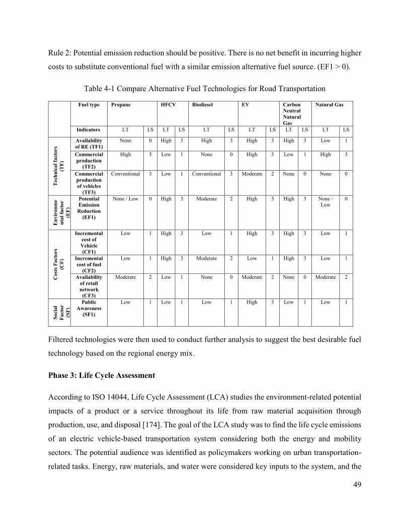
49

Rule 2: Potential emission reduction should be positive. There is no net benefit in incurring higher

costs to substitute conventional fuel with a similar emission alternative fuel source. (EF1 > 0).

Table 4-1 Compare Alternative Fuel Technologies for Road Transportation

Fuel type Propane HFCV Biodiesel EV Carbon

Neutral

Natural

Gas

Natural Gas

Indicators LT LS LT LS LT LS LT LS LT LS LT LS

Tech

nic

al

facto

rs

(TF

)

Availability

of RE (TF1)

None 0 High 3 High 3 High 3 High 3 Low 1

Commercial

production

(TF2)

High 3 Low 1 None 0 High 3 Low 1 High 3

Commercial

production

of vehicles

(TF3)

Conventional 3 Low 1 Conventional 3 Moderate 2 None 0 None 0

En

vir

on

me

nta

l fa

cto

r

(EF

)

Potential

Emission

Reduction

(EF1)

None / Low 0 High 3 Moderate 2 High 3 High 3 None / Low

0

Co

sts

Fa

cto

rs

(CF

)

Incremental

cost of

Vehicle

(CF1)

Low 1 High 3 Low 1 High 3 High 3 Low 1

Incremental

cost of fuel

(CF2)

Low 1 High 3 Moderate 2 Low 1 High 3 Low 1

Availability

of retail

network

(CF3)

Moderate 2 Low 1 None 0 Moderate 2 None 0 Moderate 2

So

cia

l

Fa

cto

r

(SF

)

Public

Awareness

(SF1)

Low 1 Low 1 Low 1 High 3 Low 1 Low 1

Filtered technologies were then used to conduct further analysis to suggest the best desirable fuel

technology based on the regional energy mix.

Phase 3: Life Cycle Assessment

According to ISO 14044, Life Cycle Assessment (LCA) studies the environment-related potential

impacts of a product or a service throughout its life from raw material acquisition through

production, use, and disposal [174]. The goal of the LCA study was to find the life cycle emissions

of an electric vehicle-based transportation system considering both the energy and mobility

sectors. The potential audience was identified as policymakers working on urban transportation-

related tasks. Energy, raw materials, and water were considered key inputs to the system, and the

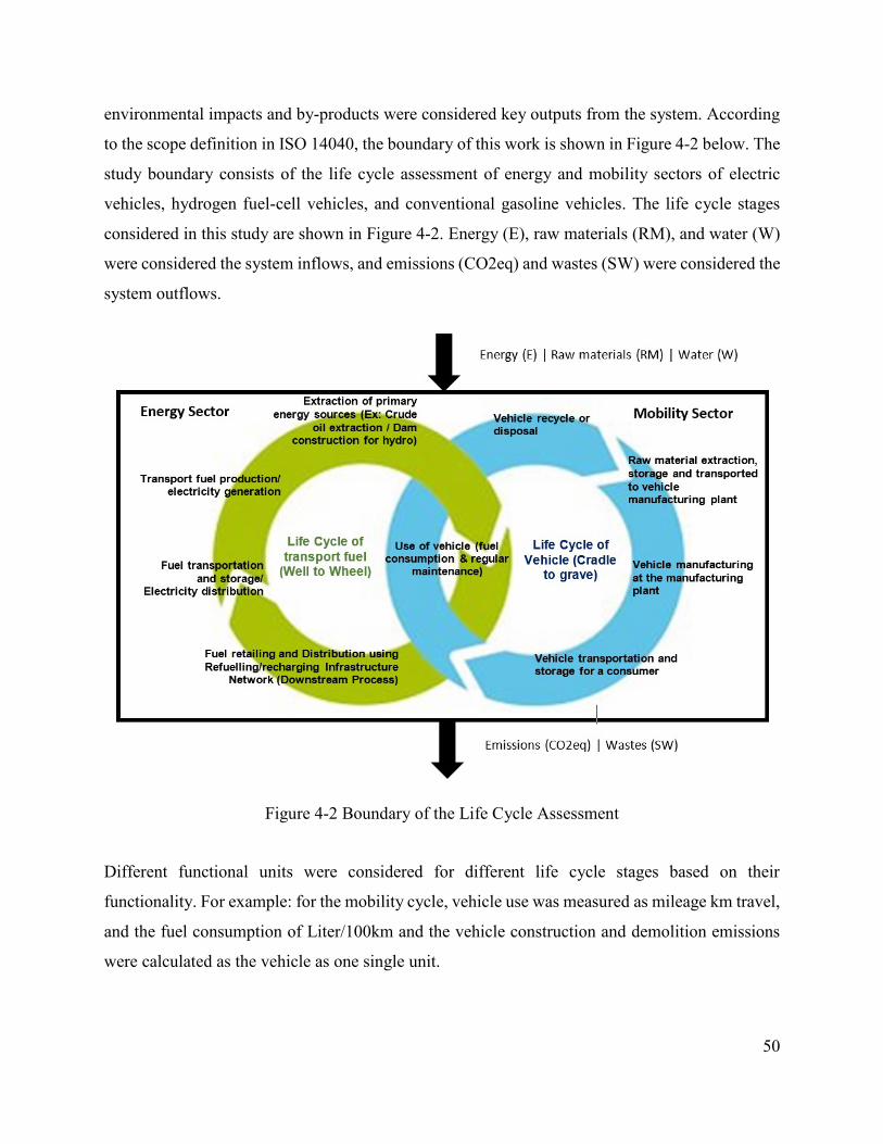
50

environmental impacts and by-products were considered key outputs from the system. According

to the scope definition in ISO 14040, the boundary of this work is shown in Figure 4-2 below. The

study boundary consists of the life cycle assessment of energy and mobility sectors of electric

vehicles, hydrogen fuel-cell vehicles, and conventional gasoline vehicles. The life cycle stages

considered in this study are shown in Figure 4-2. Energy (E), raw materials (RM), and water (W)

were considered the system inflows, and emissions (CO2eq) and wastes (SW) were considered the

system outflows.

Different functional units were considered for different life cycle stages based on their

functionality. For example: for the mobility cycle, vehicle use was measured as mileage km travel,

and the fuel consumption of Liter/100km and the vehicle construction and demolition emissions

were calculated as the vehicle as one single unit.

Figure 4-2 Boundary of the Life Cycle Assessment

51

The duration of the life cycle and the average mileage operated per year were considered to

estimate the total operational energy consumption of the vehicle within the considered life cycle.

For the energy cycle, the life cycle assessment was conducted to find the total emission of unit fuel

from well-to-pump. Ultimately, however, all those units were converted to kgCO2eq/vehicle,

considering the emissions factors for the impact category to find the total life cycle impacts of the

vehicle. In addition to that, the following assumptions were made for the life cycle assessment of

EV, HFCV, and conventional ICEV:

1. According to previous studies, the vehicle life span is considered 12-15 years [202]. However,

in this study, the vehicle use period/ life span is assumed as 5 years due to the lack of data on

maintenance after 5 years.

2. Due to the various vehicles available in the market, three specific vehicles were considered to

obtain life cycle cost data for the analysis. Those representative vehicles and the reason for

the selection are: 1) A mid-size passenger car (Nissan Leaf S 5DR) [203] (Electric), selected

based on its high market penetration as an economical EV; 2) A mid-size sports utility vehicle

(Hyundai Tucson FCEV) [204] (Hydrogen), selected because it is a popular, commercially

available vehicle in HFCV market segment; 3) A spark-ignition mid-size passenger car

(Toyota Yaris 4DR) [205], selected as the ICEV for this study due to high market penetration

as an economical vehicle and its similar engine power torque (Hp) to aforementioned

alternative vehicles.

3. The annual mileage of a vehicle in Canada is assumed as 18,000km per year [206].

In addition to the mobility cycle, the energy cycle for each energy alternative considered in this

analysis can be explained as follows:

Gasoline for transportation: Octane 85 gasoline was considered to find the life cycle inventory for

conventional ICEV refueling. The functional unit for this fuel was taken as litre fuel consumption

per 100 kilometers (l/100km). The database developed by Argonne National Laboratory was used

to collect and prepare the life cycle inventory database for gasoline fuel-based light-duty vehicles.

Hydrogen fuel-cell technology for transportation: Hydrogen fuel cell (HFC) production using

Natural Gas (NG) gasification was considered the commercially available method to produce

52

mass-scale hydrogen fuel cells for road transportation [207]. Hence, the functional unit of

hydrogen was considered as litre hydrogen fuel cells consumed per 100 kilometers (l/100km).

Furthermore, the LCA impacts of the common low-emission hydrogen production methods, which

are alkaline water electrolysis using low-emission electricity, thermochemical water splitting with

nuclear Cu-Cl cycle, and central biomass gasification, etc., were also considered in this analysis.

The database developed by the Argonne National Laboratory (2015) and other North American

databases were used to obtain data and develop the LCA databases for the analysis.

Electricity for transportation: As shown in Appendix A2, electricity generation emissions vary

with the primary energy source. The electricity mix of Canada changes by province due to the

availability of resources, raw materials, and technology. Hence, the life cycle emissions of the use

of different fuels vary with the location. The LCA inventory of grid electricity from electricity

generation to the consumer recharging point via the smart grid was calculated using GREET

software developed by Argonne National Laboratory. Different energy mixes of the electricity

generation process were defined in the aforementioned software to find the mid-point indicators

for the life cycle inventory.

The system inputs were: 1) Fossil Fuel (GJ/Unit vehicle or kJ/100litre fuel); 2) Coal Fuel (GJ/Unit

vehicle or J/100litre fuel); 3) Natural Gas Fuel (GJ/Unit vehicle or kJ/100litre fuel); 4) Petroleum

Fuel (GJ/Unit vehicle or kJ/100litre fuel); 5) Renewable (GJ/Unit vehicle or kJ/100litre fuel); 6)

Biomass (GJ/Unit vehicle or kJ/100litre fuel); 5) Nuclear (J/Unit vehicle or kJ/100litre fuel); 6)

Non-Fossil Fuel (GJ/Unit vehicle or kJ/100litre fuel); and 7) Total Water (m3/Unit vehicle or

m3/100litre fuel).

The system outputs were: 1) Volatile organic compound (VOC) (kg/Unit vehicle or mg/100litre

fuel); 2) Carbon Monoxide (CO) (kg/Unit vehicle or mg/100litre fuel); 3) Nitrogen Oxides

emissions (NOx) (kg/Unit vehicle or mg/100litre fuel); 4) Particles between 2.5 and 10 microns

(micrometers) in diameter (PM10) (kg/Unit vehicle or mg/100litre fuel); 5) Fine particulate matter

less than 2.5 micrometers in diameter (PM2.5) (kg/Unit vehicle or mg/100litre fuel); 6) Sulphur

oxides emissions (SOx) (kg/Unit vehicle or mg/100litre fuel); 7) Methane (CH4) (kg/Unit vehicle

or mg/100litre fuel); 8) Carbon Dioxide (CO2) (kg/Unit vehicle or mg/100litre fuel); 9) Nitrous

53

Oxide (N2O) (g/Unit vehicle or mg/100litre fuel); 10) Bio Carbon (BioC) (g/Unit vehicle or

mg/100litre fuel); and 11) Particle Oxidation Catalysts (POC) (g/Unit vehicle or mg/100litre fuel).

Equation (14) was used to find operational emissions based on the emissions of unit fuel

consumption.

𝐸(𝑟𝑒𝑐𝑢𝑟𝑟𝑖𝑛𝑔) = 𝛾 × 𝐴𝑀 × 𝐿𝑇 𝑉𝐹𝐶⁄ Equation 14

Where, E(recurring) – Vehicle operation (fuel) emissions (kgCO2e); 𝛾 – Emission factor

(emissions per unit fuel); AM – Annual mileage (km/year); LT – life span (year); VFC – Fuel

consumption (km/per unit fuel)

The vehicle (from cradle-to-grave) with fuel (from well-to-pump) was considered for the complete

life cycle of the mobility and energy cycles, used to describe the total emissions related to road

transportation [177]. Hence, the life cycle of the overall system was described as Equation (15).

The possible light-duty vehicle options were developed accordingly, using different fuel-

production methods, regional energy-mixes, and commercial availability of mass fuel sources. The

options considered in this work including hydrogen fuel cell vehicles with different hydrogen fuel

production methods, EVs with different grid-mixes within Canada, and conventional gasoline fuel-

based vehicles (ICEVs).

LCA_S = LCA_V + LCA_Fw2p Equation 15

Where, LCA_S – Life cycle emissions of the system (vehicle life cycle & fuel life cycle)

(kgCO2e); LCA_V – Life cycle emissions of the vehicle (kgCO2e)*; LCA_Fw2p – Life cycle

emissions of fuel from well to wheel (kgCO2e)**

The impacts of the inventory were then organized into impact categories. Literature-based

inventory-impact conversion factors obtained from the study conducted by Asdrubali, F., et al.

(2015), were used to find LCA impacts of each impact category [208]. The mid-point indicators

were considered in this chapter to show the relationship to emission flows and used for further

comparison. Hauschild, M., H., and Huijbregts, M., A., J., (2015) showed a comparison of mid-

point indicators and end-point indicators where the mid-point indicators are highly suitable to show

elementary flows and lower modeling uncertainty [209]. The following mid-point impact

54

categories were considered in this analysis and will be most affected by local communities in the

long-run [210] [211]. There are: 1) Global warming potential (GWP); 2) Photochemical ozone

formation (POF); 3) Acidification of land and water (ALW); 4) Eutrophication (EN); 5)

Stratospheric ozone depletion (SOD); and 6) Depletion of non-renewable energy resources (DNR).

Phase 4: Life Cycle Cost Assessment

According to the available literature, life cycle cost (LCC) can be explained as the complete costs

of a vehicle in its entire life span. Typically, the vehicle life cycle cost varies with the vehicle type,

use behaviours, local fuel prices, other vehicle costs, and vehicle end-of-life cost. Generally, the

vehicle shows negative end-of-life cost (positive income), which reduces the overall life cycle cost.

The LCC for the vehicle can be expressed as Equation (16) [179].

LCCVehicle = Vcapex + Vopex + VEoL Equation 16

Where, LCCvehicle = Life cycle cost of the vehicle (CAD/vehicle); Vcapex = Vehicle capital

expenditure / purchasing price (CAD/vehicle); Vopex = Present value of the all operational

expenditure (CAD/vehicle); VEoL = Vehicle end-of-life costs (CAD/vehicle)

The data provided in Table 4-2 was used to calculate the vehicle capital expenditure (CAPEX),

operational expenditure (OPEX), and vehicle end-of-life costs (EoL). The operational cost was

calculated using Equation (17).

Vopex = VOC + VM&RC + EVBC Equation 17

Where, Vopex = Present value of the all operational expenditure (CAD/vehicle); Voc = Present value

of the operating costs (CAD/vehicle.lifecycle); VM&RC = Present value of the maintenance and

repair cost (CAD/vehicle.lifecycle); EVBC = Cost of electric vehicle battery replacement (EVBC)

– (CAD/battery.life cycle)

The vehicle operating costs and electric vehicle battery replacement costs were calculated as

Equation (18) and Equation (19), respectively.

55

VOC = Fc . AM VFC⁄ Equation 18

Where, Voc = Vehicle operating cost (CAD/vehicle.life cycle); Fc = Fuel or electric cost of the

considered region (CAD/litre or CAD/kwh); AM = Average annual millage travel

(km/year.vehicle); VFC = Vehicle fuel / electricity consumption (Litres/100km or km/kWh)

EVBC = CF. EVCB. AM EVBRC. Rng⁄ Equation 19

Where, CF= Cost factor for EV battery – (CAD 300 /kWh [212]); EVCB = Capacity of battery –

30kWh (see Annexure D); EVBRC = No. of re-charging cycles in battery life cycle – Li-ion battery

with 3,000 cycles; Rng = Vehicle range per one recharging cycle (km/cycle); AM = Average

annual millage travel (km/year.vehicle)

The Net Present Value (NPV) was calculated using Equation (20) [180] in order to compare the

costs of different vehicles.

NPV(i, N) = ∑ Rt (1 + i)t⁄Nt=0 Equation 20

Where, NPV = Net Present Value (CAD), Rt = Net cash flow (CAD); i = Discount rate (%); N =

Study period (Years); t = Time of the cash flow

The cost data of the considered vehicles are given in Table 4-2. The full collection of the data is

attached as appendices, as stated in Table 4-2. The vehicle purchase price (in British Columbia,

Canada) was considered as the product purchase cost or the initial investment. Operational

expenses such as fuel expenses and maintenance and repair expenses were considered as recurring

costs. Additionally, end-of-life cost after the life of the vehicle was considered positive, which is

generally a gain to the consumer.

56

Table 4-2 Life Cycle Cost Calculation for the System (LCC_S)

Gasoline Hydrogen Electricity

Vehicle purchase price (C)

Vehicle capital expenditure

/ purchasing price (Vcapex)

CAD 21,151/vehicle CAD 66,940/vehicle5 CAD 26,688/Vehicle

Vehicle operational and maintenance cost (PVrecurring)

Fuel or electric cost (Fc) Refer Appendix A4 Provincial data not

available. The average

price is CAD 5 per kg

Hydrogen [213]

Refer Appendix A3 and

retailor margin of CAD

0.02915/ kWh.

Fuel consumption rate (Vfc) 12.32 km per Liter of

Gasoline

77 km per kg of

Hydrogen 34 kWh per 100km

Maintenance and repair cost

(VM&RC)

Refer Appendix B1 Refer Appendix B1 Refer Appendix B1

Cost of Battery Replacement

(EVBC)

Negligible Negligible CAD 406 /

(year.vehicle)

Vehicle residual value (PVresidual-value)

End-of-life cost CAD 8,006 CAD 20,082 CAD 6,345

The following assumptions were made to perform necessary LCC calculations.

1. The insurance costs of the vehicles depend on the valuation of the vehicle, driver, policies,

and vehicle use [214]. Therefore, insurance costs have not been considered for the LCC of

vehicles.

2. The regional hydrogen production method was assumed based on the availability of green

electricity and natural gas in a particular region.

3. The vehicle end-of-life cost was assumed as 30% of the vehicle purchasing cost.

4. Assumed 10 year payback period for EV infrastructure facility and zeroed residual value

after ten years lifetime.

5. EV re-charging facility operates with an 80% efficiency rate for 16 hours per day and 365

days per year. The public re-charging station capacity was assumed as 50kW [215].

5 Includes fuel cost, maintenance and repair cost for first 03 years. Please see Appendix B1.

57

6. The consumer price index for Canada is 2% [113], and the discount rate for Canada is taken

as 3.5% (Innovation, Science and Economic Development Canada, 2014) for annualizing

the cost factors.

7. The retailer’s profit mark-up was assumed as 12%.

8. Average cost of level III facility is CAD 35,000 to 45,000 per facility [87].

9. CAD 2,000 per year without including the cost of energy [217].

According to the aforementioned methodology, the overall life cycle cost of each fuel option was

calculated based on the provincial data obtained in Canada.

Phase 5: Select the most desirable alternative fuel option for road transportation

This section explains the methodology used to select the best desirable fuel option for road

transportation considering regional economic and environmental parameters of the available fuel

options. As the first stage, the alternative fuel options were defined using different combinations

considering the regional fuel availability. Those were coded as follows to enhance the clarity of

the explanation.

OP1_EV EVs operated using the provincial grid electricity (Central)

OP2_EV EVs operated using renewable energy such as Solar(PV), wind, etc. (Distributed)

OP3_HFCV HFCVs operated using hydrogen fuel cells (HFCs) produced by the provincial

grid electricity (Central)

OP4_HFCV HFCVs operated using HFCs produced by water electrolysis using renewable

energy such as Solar(PV), wind, etc. (Distributed)

OP5_HFCV HFCVs operated using HFCs produced by central coal gasification (Central)

OP6_HFCV HFCVs operated using HFCs produced by biomass gasification (Distributed)

OP7_HFCV HFCVs operated using HFCs produced by thermochemical water splitting with

nuclear Cu–Cl cycle (Central)

OP8_HFCV HFCVs operated using Canadian natural gas-based HFCs Production (Central)

BC_ICEV The conventional use of ICEVs using gasoline as the fuel source

58

The mid-point impacts identified from the LCA to obtain the damage impacts to the environment

were calculated for the options mentioned above (including the conventional fuel-based vehicles).

Mid-point indicators were compared and conclusions were given considering environmental

perspective. However, the comparison showed different options for different indicators. Therefore,

the environmental score was defined to obtain a single value for each considered option to compare

and select the most desirable vehicle option.

The single life cycle impact index obtained using Netherlands Oil and Gas Exploration and

Production Association (NOGEPA) suggested weights can be defined as the “Environmental Score

(EnvS)” for each alternative fuel option. NOGEPA weights were selected from the literature to

indicate the relative importance of each impact indicator considering the industrial (oil and gas)

applicability and appropriateness of those weights for the eco-efficiency-based studies [218]. The

NOGEPA weights for GWP, SOD, ALW, EN, POF, and DNR were considered as 32, 5, 6, 13, 8,

and 8, respectively [218]. The indicator values were normalized using Equation (21) prior to

multiplying with the NOGEPA weights.

Xi,normalized = (xi,j − xi,min) (xi,max − xi,min)⁄ Equation 21

Where, X I,normalized – Normalized value for the alternative I and indicator j; Xi,j – Value given in

alternative I and indicator j; Xi,min – Value given in alternative I and minimum value of indicator j;

Xi,max – Value given in alternative I and maximum value of indicator j

The normalized mid-point impacts were then multiplied with NOGEPA weights and aggregated

to obtain a single impact per each alternative fuel option [219]. LCC for the aforementioned fuel

options were also assessed and normalized in order to obtain the “Economic Score (EconS)” of

the different alternative fuel options. Equation (21) was used to normalize the LCC values, and the

normalized values were aggregated to find the economic score.

EnvS and EconS were compared individually and discussed the appropriateness of each fuel option

in different provinces. A single indicator-based eco-efficiency analysis was conducted to evaluate

and obtain the most desirable alternative fuel type for a given region, considering the economic

and environmental perspective. Equation (22) was used to calculate the eco-efficiency of the

selected fuel option.

59

Eco − efficiency score = EnvS EconS⁄ Equation 22

Where, EnvS – Environmental score; EconS – Economic score

Accordingly, the most desirable fuel options were determined for each province in Canada.

4.3 Results and Discussion

The Canadian federal government and provincial governments are more concerned with reduction

of transport-based GHG emissions, which will eventually lead to achieving provincial greenhouse

gas reduction targets. This section discusses the results of the aforementioned study. Accordingly,

the alternative fuel options for Canada were assessed using the rule-based method, and EVs and

HFCVs were chosen based on their appropriateness. Afterward, the EVs and HFCVs were further

analyzed with a detailed LCC and LCA. Different regional energy mixes and technologies were

considered in this analysis. The results obtained from the LCC, LCA and enhanced LCC

calculations are described in this section. Light-duty vehicles operated using electricity, hydrogen

fuel cells, and gasoline were compared with each other.

4.3.1 Life Cycle Inventory for Different Fuel Options and Different Mixes of the Source

Energy

The life cycle inventory results for hydrogen fuel cell vehicles, electric vehicles, and conventional

vehicles are shown in Table 4-3. In this analysis, the fuel cycle was not considered and the vehicle

cradle-to-grave was considered without the operational emissions. Table 4-3 shows the resource

required to manufacture vehicles, and resultant emissions are significantly higher than the vehicle

maintenance and end-of-life phase. Conventional vehicles show the lowest manufacturing

emissions in almost all categories, whereas EVs show the highest manufacturing emissions in most

emission categories. However, operational emissions need to be integrated into the above life cycle

values to identify the most desirable vehicle categories. Hence, cradle-to-grave emissions of

hydrogen fuel cells and electricity are shown in Table 4-4 and Table 4-5, respectively.

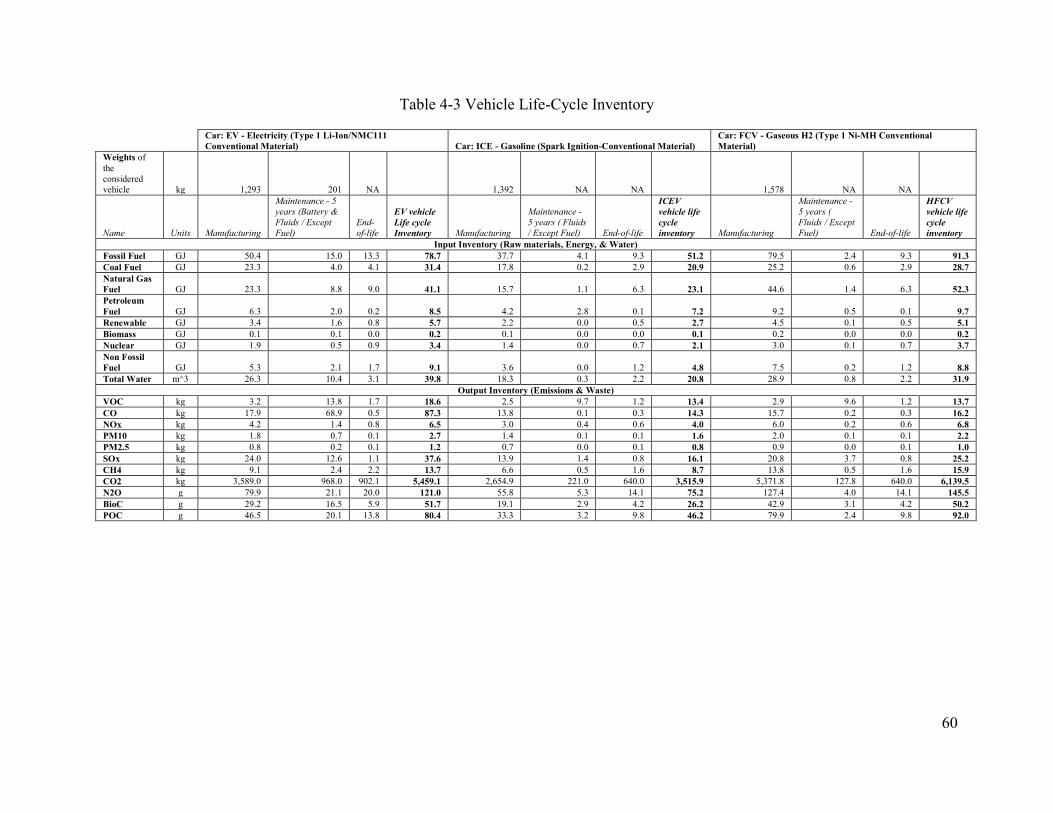
60

Table 4-3 Vehicle Life-Cycle Inventory

Car: EV - Electricity (Type 1 Li-Ion/NMC111

Conventional Material) Car: ICE - Gasoline (Spark Ignition-Conventional Material)

Car: FCV - Gaseous H2 (Type 1 Ni-MH Conventional

Material)

Weights of

the

considered

vehicle kg 1,293 201 NA 1,392 NA NA 1,578 NA NA

Name Units Manufacturing

Maintenance - 5

years (Battery &

Fluids / Except

Fuel)

End-

of-life

EV vehicle

Life cycle

Inventory Manufacturing

Maintenance -

5 years ( Fluids

/ Except Fuel) End-of-life

ICEV

vehicle life

cycle

inventory Manufacturing

Maintenance -

5 years (

Fluids / Except

Fuel) End-of-life

HFCV

vehicle life

cycle

inventory

Input Inventory (Raw materials, Energy, & Water)

Fossil Fuel GJ 50.4 15.0 13.3 78.7 37.7 4.1 9.3 51.2 79.5 2.4 9.3 91.3

Coal Fuel GJ 23.3 4.0 4.1 31.4 17.8 0.2 2.9 20.9 25.2 0.6 2.9 28.7

Natural Gas

Fuel GJ 23.3 8.8 9.0 41.1 15.7 1.1 6.3 23.1 44.6 1.4 6.3 52.3

Petroleum

Fuel GJ 6.3 2.0 0.2 8.5 4.2 2.8 0.1 7.2 9.2 0.5 0.1 9.7

Renewable GJ 3.4 1.6 0.8 5.7 2.2 0.0 0.5 2.7 4.5 0.1 0.5 5.1

Biomass GJ 0.1 0.1 0.0 0.2 0.1 0.0 0.0 0.1 0.2 0.0 0.0 0.2

Nuclear GJ 1.9 0.5 0.9 3.4 1.4 0.0 0.7 2.1 3.0 0.1 0.7 3.7

Non Fossil

Fuel GJ 5.3 2.1 1.7 9.1 3.6 0.0 1.2 4.8 7.5 0.2 1.2 8.8

Total Water m^3 26.3 10.4 3.1 39.8 18.3 0.3 2.2 20.8 28.9 0.8 2.2 31.9

Output Inventory (Emissions & Waste)

VOC kg 3.2 13.8 1.7 18.6 2.5 9.7 1.2 13.4 2.9 9.6 1.2 13.7

CO kg 17.9 68.9 0.5 87.3 13.8 0.1 0.3 14.3 15.7 0.2 0.3 16.2

NOx kg 4.2 1.4 0.8 6.5 3.0 0.4 0.6 4.0 6.0 0.2 0.6 6.8

PM10 kg 1.8 0.7 0.1 2.7 1.4 0.1 0.1 1.6 2.0 0.1 0.1 2.2

PM2.5 kg 0.8 0.2 0.1 1.2 0.7 0.0 0.1 0.8 0.9 0.0 0.1 1.0

SOx kg 24.0 12.6 1.1 37.6 13.9 1.4 0.8 16.1 20.8 3.7 0.8 25.2

CH4 kg 9.1 2.4 2.2 13.7 6.6 0.5 1.6 8.7 13.8 0.5 1.6 15.9

CO2 kg 3,589.0 968.0 902.1 5,459.1 2,654.9 221.0 640.0 3,515.9 5,371.8 127.8 640.0 6,139.5

N2O g 79.9 21.1 20.0 121.0 55.8 5.3 14.1 75.2 127.4 4.0 14.1 145.5

BioC g 29.2 16.5 5.9 51.7 19.1 2.9 4.2 26.2 42.9 3.1 4.2 50.2

POC g 46.5 20.1 13.8 80.4 33.3 3.2 9.8 46.2 79.9 2.4 9.8 92.0

61

Table 4-4 Electricity (Generation to Recharging) Life-Cycle Inventory

Input Inventory

(Raw materials |

Energy | Water)

Province-wise grid-electricity generation (Unit impact per MJ electricity)

Unit

British

Columbia Manitoba Quebec

Newfoundland

and Labrador Yukon

Northwest

Territories Ontario

New

Brunswick Saskatchewan

Nova

Scotia Alberta

Prince

Edward

Island Nunavut

Water m^3 0.004251 0.494 0.0044 0.0044 0.0043 0.0021 0.0015 0.0012 0.00093 0.000751 0.000035 0.0000107 0.001954

Non fossil fuels KJ 1,192 1,000 1,035 950.61 920.92 418.25 988.17 804.42 180.99 439.09 171.93 1,025 53.68

Renewable KJ 1,192 1,000 1,035 950.27 920.41 413.7 396.57 442.54 180.45 437.53 171.15 1,025 24.05

Biomass KJ 271.5 0 45.25 0.001 0.016 145.83 45.3 181.06 0.017 226.3 90.53 45.25 0.949

Fossil Fuels KJ 61.61 0 1.14 154.01 241.86 1906 125.74 949.36 2105 2075 2312 34.22 12,000

Petroleum Fuels KJ 36.35 0 1 121.14 181.76 1665 2929.06 254.7 21.43 389.39 114.09 31.27 11,000

Natural Gas

Fuels KJ 24.79 0 0.012 31.44 57.94 221.89 115.76 242.11 803.63 345.35 944.46 2.59 8875

Coal Fuels J 460.07 0 13.61 1,427.03 2,154.97 19340 7,055.08 452,550 1,280,000 1,340,000 1,253,000 363 125.8

Nuclear J 107.99 0 3.19 335.76 506.92 4,552.8 591,600 361,880 0.544 1,564.47 788.22 85.5 29.63

Output Inventory

(Emissions |

Waste)

Province-wise grid-electricity generation (Unit impact per MJ electricity)

Unit

British

Columbia Manitoba Quebec

Newfoundland

and Labrador Yukon

Northwest

Territories Ontario

New

Brunswick Saskatchewan

Nova

Scotia Alberta

Prince

Edward

Island Nunavut

Total CO2 g 0.51 0 0.058 0.012 18.25 150 7.37 20.83 170 54.66 180 2.69 950

VOC mg 0.11 0 0.41 1.02 1.63 12.04 1.88 0.77 16.57 1.29 18.85 0.62 73.52

CO mg 1.27 0 13.18 3.62 5.89 40.78 19.62 3.92 54.96 6.57 90.51 13.86 240

NOX mg 0.67 0 2.9 48.47 73.27 660 11.11 10.42 120 24.37 170 14.73 4260

PM10 mg 0.48 0 5.78 2.06 3.11 27.99 6.14 1.59 19.82 3.85 32.73 6.29 180

PM2.5 mg 0.16 0 1.7 1.5 2.27 20.29 1.98 1.03 8.59 2.61 13.16 2.06 130

SOX mg 0.36 0 1.81 33.1 50.68 460 4.94 41.7 310 120 330 10.17 3010

CH4 mg 0.25 0 1.47 15.44 24.99 180 22.7 1.41 240 1.69 260 4.41 1060

N2O mg 0.02 0 0.18 0.11 0.17 1.3 0.29 0.3 3.15 0.8 3.74 6.21 8.05

BioC mg 0.02 0 0.24 0.12 0.18 1.57 0.3 0.069 0.56 0.15 1.16 0.27 10.09

POC mg 0.05 0 0.55 0.14 0.21 1.7 0.66 0.16 1.43 0.32 2.71 0.58 10.68

H2 mg 0 0 0 0 0 0 0 0 0 0 0 0 0

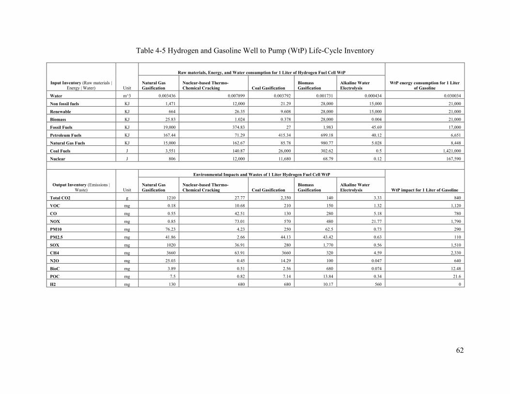
62

Table 4-5 Hydrogen and Gasoline Well to Pump (WtP) Life-Cycle Inventory

Input Inventory (Raw materials |

Energy | Water) Unit

Raw materials, Energy, and Water consumption for 1 Liter of Hydrogen Fuel Cell WtP

WtP energy consumption for 1 Liter

of Gasoline

Natural Gas

Gasification

Nuclear-based Thermo-

Chemical Cracking Coal Gasification

Biomass

Gasification

Alkaline Water

Electrolysis

Water m^3 0.003436 0.007899 0.003792 0.001731 0.000434 0.030034

Non fossil fuels KJ 1,471 12,000 21.29 28,000 15,000 21,000

Renewable KJ 664 26.35 9.608 28,000 15,000 21,000

Biomass KJ 25.83 1.024 0.378 28,000 0.004 21,000

Fossil Fuels KJ 19,000 374.83 27 1,983 45.69 17,000

Petroleum Fuels KJ 167.44 71.29 415.34 699.18 40.12 6,651

Natural Gas Fuels KJ 15,000 162.67 85.78 980.77 5.028 8,448

Coal Fuels J 3,551 140.87 26,000 302.62 0.5 1,421,000

Nuclear J 806 12,000 11,680 68.79 0.12 167,590

Output Inventory (Emissions |

Waste) Unit

Environmental Impacts and Wastes of 1 Liter Hydrogen Fuel Cell WtP

WtP impact for 1 Liter of Gasoline

Natural Gas

Gasification

Nuclear-based Thermo-

Chemical Cracking Coal Gasification

Biomass

Gasification

Alkaline Water

Electrolysis

Total CO2 g 1210 27.77 2,350 140 3.33 840

VOC mg 0.18 10.68 210 150 1.32 1,120

CO mg 0.55 42.51 130 280 5.18 780

NOX mg 0.85 73.01 570 480 21.77 1,790

PM10 mg 76.23 4.23 250 62.5 0.73 290

PM2.5 mg 41.86 2.66 44.13 43.42 0.63 110

SOX mg 1020 36.91 280 1,770 0.56 1,510

CH4 mg 3660 63.91 3660 320 4.59 2,330

N2O mg 25.03 0.45 14.29 100 0.047 640

BioC mg 3.89 0.51 2.56 680 0.074 12.48

POC mg 7.5 0.82 7.14 13.84 0.34 21.6

H2 mg 130 680 680 10.17 560 0

63

Table 4-4 shows the topological variations of cradle-to-grave resource consumption and resultant

emissions for grid electricity due to different energy mixes in different provinces. Manitoba,

British Columbia, Quebec, and Prince Edward Island show lower consumption of non-renewable

energy and result in lower emissions compared with Saskatchewan, Alberta, Nunavut, and the

Northwest Territories. Table 4-5 shows the fuel life cycle for hydrogen fuel cells. Accordingly,

alkaline water electrolysis using renewable energy sources has the lowest resource consumption

and emissions, followed by the gasification of biomass, natural gas, coal, and nuclear-based

thermo-chemical cracking. The carbon-capturing techniques for HFC production were not

considered in this analysis due to a lack of available data.

According to the life cycle inventory information, the following comparisons were conducted and

the results of the same are given as follows:

1. Vehicle cradle-to-gate environmental impacts - To identify the alternative vehicle category

that emits the highest emissions in its production process.

2. Vehicle cradle-to-grave environmental impacts – To identify the alternative vehicle

categories that emit the highest emissions in their entire life cycle. This includes fuel-based

emissions from well-to-wheel.

4.3.2 Compare Vehicle Options using Cradle-to-Gate Emissions

Cradle-to-gate emissions of the selected alternative fuel-based vehicles were compared in this

section to identify the production emissions of the considered vehicle options. The following

vehicle manufacturing emissions, including vehicle battery-based emissions, were considered in

the analysis: VOC, CO, NOx, PM10, PM2.5, SOx, CH4, CO2, N2O, BC or BioC, and POC. The

conversion factors below were used to convert the emissions mentioned above into mid-point

indicators [209] [220].

Depletion of non-renewable resources is a cumulative total of fossil fuels, 6.12 times of

petroleum fuels, 7.8 times of natural gas fuels, and 0.25 times of coal fuels.

Global warming potential is a cumulative total of total CO2 emissions, 28 times of CH4, and

265 times of N2O.

64

Photochemical ozone creation is a cumulative total of 0.416 times of VOC, 0.036 of CO, and

0.007 times of CH4.

Eutrophication is a cumulative total of 0.04 times of NOx and 0.09 times of N2O.

Acidification and land and water is a cumulative total of 40.04 times of NOx and 50.79 times

of SOx.

The mid-point indicator values were considered to compare both EVs and HFCVs based on their

cradle-to-gate emissions, which are shown in Figure 4-3.

Figure 4-3 Cradle-to-gate Emission of Alternative Fuel-based Vehicle Options

As indicated, EVs and HFCVs contribute to the environment differently. On one hand, resource

consumption is higher in HFCVs than EVs, and therefore more resources are needed to

manufacture an HFCV than an EV. HFCV manufacturing enhances global warming and

eutrophication compared to similar EVs. On the other hand, EVs emit a higher amount of photo-

oxidants and acids to the environment compared with HFCV as a result of the emissions created

by the EV battery. The NOGEPA weights were used to develop a single environmental score for

each HFCV and EV cradle-to-gate emissions to compare both vehicles. The environmental scores

were calculated as 56.22 for the HFCV and 48.78 for the EV. Accordingly, the cradle-to-gate

emissions of EVs are considerably higher than similar ICEVs, which is slightly lower than a similar

HFCVs. However, these emissions can be lowered with technological advancements such as low

0% 10% 20% 30% 40% 50% 60% 70% 80% 90% 100%

Acdification land and water

Eutrophication

Global Warming Potential

Photochemical Ozone Creation

Depletion of non-renewable energy resources

EV cradle-to-gate emissions HFCV cradle-to-gate emissions

65

emission production methods, high recycling and reuse of materials, carbon-capturing

technologies, etc. in the future.

4.3.3 Compare Vehicles using Cradle-to-Grave Emissions

The vehicle cradle-to-gate emissions, operational emissions including the wheel to pump

emissions of the fuel, and vehicle end-of-life emissions were considered in this analysis. The

cradle-to-grave LCA mid-point indicators for EVs and HFCVs were compared to each other to

observe the environmental appropriateness of each fuel option, to replace conventional fuels in the

long run. The comparison is shown in Figure 4-4 for different fuel options.

According to the analysis, the OP4_HFCV, OP2_EV, and OP7_HFCV showed lower emissions

in all provinces. However, OP4_HFCV and OP2_EV need nearly zero-emission electricity to

achieve the given emission targets, which might not be an ideal option for most of those provinces

due to the lack of renewable resources. OP7_HFCV requires HFCVs to operate using HFCs

produced by thermochemical water splitting with nuclear Cu–Cl cycle, which is a significantly

higher cost option. The above transport options need green electricity, while some provinces have

minimal renewable options due to lack of resources, investments, and technology know-how.

The OP1_EV, OP3_HFCV, OP5_HFCV, and OP6_HFCV showed comparatively better

environmental performances except for the Northwest Territories, Saskatchewan, Nova Scotia,

Alberta, and Nunavut. Moreover, ICEV-based conventional transportation showed a negative

impact on the environment in all provinces except Nunavut. To analyze this further, an

environmental index for each fuel option was calculated, as discussed in the methodology.

Accordingly, the OP2_EV, OP4_HFCV, and OP7_HFCV were considered optimistic options,

though they are beyond the current scope of the work. OP1_EV, OP3_HFCV, OP6_HFCV,

OP5_HFCV, and OP8_HFCV were considered as most likely fuel options that are viable to

achieve within the foreseeable future. Conventional fuel was considered the pessimistic fuel

option, which can be continued if other options fail in the deployment process.

66

Figure 4-4 Mid-point Indicators for Alternative Fuel Options

OP1_EV OP2_EV OP3_HFCV OP4_HFCV OP5_HFCV OP6_HFCV OP7_HFCV OP8_HFCV BC_ICEVBRITISH COLUMBIAALW 0.28 0.28 0.00 0.00 0.28 0.84 0.03 0.40 1.00EN 0.07 0.00 0.00 0.00 0.17 0.20 0.02 0.01 1.00GLW 0.00 0.00 0.01 0.00 1.00 0.07 0.02 0.54 0.78POF 0.27 0.27 0.00 0.00 0.11 0.07 0.01 0.02 1.00DNR 0.02 0.00 0.03 0.00 0.27 0.10 0.02 1.00 0.90MANITOBAALW 0.28 0.28 0.00 0.00 0.28 0.84 0.03 0.40 1.00EN 0.00 0.01 0.01 0.01 0.18 0.21 0.03 0.02 1.00GLW 0.00 0.02 0.02 0.02 1.00 0.09 0.03 0.55 0.79POF 0.27 0.27 0.00 0.00 0.11 0.07 0.01 0.02 1.00DNR 0.00 0.00 0.00 0.00 0.27 0.10 0.02 1.00 0.90QUEBECALW 0.29 0.28 0.01 0.00 0.28 0.84 0.03 0.40 1.00EN 0.00 0.01 0.01 0.01 0.17 0.20 0.02 0.02 1.00GLW 0.00 0.02 0.02 0.02 1.00 0.09 0.03 0.55 0.79POF 0.28 0.27 0.01 0.00 0.11 0.07 0.01 0.02 1.00DNR 0.00 0.00 0.00 0.00 0.27 0.10 0.02 1.00 0.90NEWFOUNDERLAND & LABRADORALW 0.47 0.28 0.23 0.00 0.28 0.84 0.03 0.40 1.00EN 0.08 0.00 0.12 0.00 0.17 0.20 0.02 0.01 1.00GLW 0.00 0.02 0.02 0.02 1.00 0.09 0.03 0.54 0.79POF 0.28 0.27 0.01 0.00 0.11 0.07 0.01 0.02 1.00DNR 0.06 0.00 0.07 0.00 0.27 0.10 0.02 1.00 0.90YUKONALW 0.57 0.28 0.36 0.00 0.28 0.84 0.03 0.40 1.00EN 0.13 0.00 0.18 0.00 0.17 0.20 0.02 0.01 1.00GLW 0.03 0.00 0.07 0.00 1.00 0.07 0.01 0.54 0.78POF 0.28 0.27 0.01 0.00 0.11 0.07 0.01 0.02 1.00DNR 0.09 0.00 0.11 0.00 0.27 0.10 0.02 1.00 0.90NORTHWEST TERRITORIESALW 0.89 0.09 1.00 0.00 0.09 0.26 0.01 0.12 0.31EN 0.79 0.00 1.00 0.00 0.11 0.12 0.01 0.01 0.63GLW 0.40 0.00 0.53 0.00 1.00 0.07 0.01 0.54 0.78POF 0.32 0.27 0.06 0.00 0.11 0.07 0.01 0.02 1.00DNR 0.67 0.00 0.84 0.00 0.27 0.10 0.02 1.00 0.90ONTARIOALW 0.32 0.28 0.05 0.00 0.28 0.84 0.03 0.40 1.00EN 0.01 0.00 0.03 0.00 0.17 0.20 0.02 0.01 1.00GLW 0.00 0.00 0.03 0.00 1.00 0.07 0.01 0.54 0.78POF 0.28 0.27 0.01 0.00 0.11 0.07 0.01 0.02 1.00DNR 0.05 0.00 0.07 0.00 0.27 0.10 0.02 1.00 0.90NEWBRUNSWICKALW 0.41 0.28 0.16 0.00 0.28 0.84 0.03 0.40 1.00EN 0.01 0.00 0.03 0.00 0.17 0.20 0.02 0.01 1.00GLW 0.04 0.00 0.07 0.00 1.00 0.07 0.01 0.54 0.78POF 0.28 0.27 0.00 0.00 0.11 0.07 0.01 0.02 1.00DNR 0.22 0.00 0.28 0.00 0.27 0.10 0.02 1.00 0.90SASKATCHEWANALW 1.00 0.21 0.99 0.00 0.21 0.62 0.02 0.29 0.74EN 0.23 0.00 0.30 0.00 0.17 0.20 0.02 0.01 1.00GLW 0.46 0.00 0.60 0.00 1.00 0.07 0.01 0.54 0.78POF 0.34 0.27 0.09 0.00 0.11 0.07 0.01 0.02 1.00DNR 0.43 0.00 0.54 0.00 0.27 0.10 0.02 1.00 0.90NOVA SCOTIAALW 0.65 0.28 0.46 0.00 0.28 0.84 0.03 0.40 1.00EN 0.04 0.00 0.06 0.00 0.17 0.20 0.02 0.01 1.00GLW 0.13 0.00 0.19 0.00 1.00 0.07 0.01 0.54 0.78POF 0.28 0.27 0.01 0.00 0.11 0.07 0.01 0.02 1.00DNR 0.36 0.00 0.46 0.00 0.27 0.10 0.02 1.00 0.90ALBERTAALW 0.98 0.18 1.00 0.00 0.18 0.55 0.02 0.26 0.65EN 0.33 0.00 0.43 0.00 0.17 0.20 0.02 0.01 1.00GLW 0.49 0.00 0.64 0.00 1.00 0.07 0.01 0.54 0.78POF 0.36 0.27 0.11 0.00 0.11 0.07 0.01 0.02 1.00DNR 0.52 0.00 0.65 0.00 0.27 0.10 0.02 1.00 0.90PRINCE EDWARD ISLANDALW 0.34 0.28 0.07 0.00 0.28 0.84 0.03 0.40 1.00EN 0.04 0.00 0.07 0.00 0.17 0.20 0.02 0.01 1.00GLW 0.00 0.01 0.02 0.01 1.00 0.08 0.02 0.54 0.78POF 0.28 0.27 0.01 0.00 0.11 0.07 0.01 0.02 1.00DNR 0.01 0.00 0.02 0.00 0.27 0.10 0.02 1.00 0.90NUNAVUTALW 0.81 0.01 1.00 0.00 0.01 0.04 0.00 0.02 0.05EN 0.80 0.00 1.00 0.00 0.02 0.02 0.00 0.00 0.10GLW 0.79 0.00 1.00 0.00 0.30 0.02 0.00 0.16 0.23POF 0.58 0.27 0.38 0.00 0.11 0.07 0.01 0.02 1.00DNR 0.80 0.00 1.00 0.00 0.03 0.01 0.00 0.11 0.10

67

These normalized indicators were multiplied by NOGEPA weights and aggregated to find the

environmental score of different fuel options. Figure 4-5 shows the environmental score of

different fuel options for different provinces. Accordingly, OP1_EV, OP3_HFCV, and

OP6_HFCV were shown as better fuel options for British Columbia, Manitoba, Quebec,

Newfoundland and Labrador, Yukon, Ontario, New Brunswick, Nova Scotia, and Prince Edward

Island. Only OP6_HFCV was shown as a better option for Saskatchewan, Northwest Territories,

Alberta, and Nunavut.

Figure 4-5 Environmental Scores of Alternative Fuel Options (Most Likely and Conventional)

Accordingly, EV operation emissions are highly dependent on the provincial grid-electricity mix

and the emissions of the HFCVs highly depend on the primary energy source that is used to

produce hydrogen fuel cells. The provinces with low-emission electricity such as Manitoba, British

Columbia, Quebec, and Prince Edward Island, show high potential for EVs. Moreover, the use of

HFCVs powered by hydrogen fuel-cells produced using alkaline water electrolysis from low-

emission electricity shows the lowest impact compared to other alternative vehicle options.

However, the mass production and distribution of hydrogen fuel cell energy needs to be developed

throughout the country in a cost-effective manner. Therefore, the LCC of the aforementioned fuel

options needs to be considered in decision making on a sustainable alternative fuel option for the

68

future. Hence, the LCC-based cost parameter would benefit from selecting the final alternative

fuel option for Canadian provinces.

4.3.4 Life Cycle Costs of Different Fuel Options

Generally, the switching cost of the vehicle, infrastructure, and operational expenditure are high

when substituting conventional products with innovative products. For alternative fuel vehicles,

the daily operating cost consists of vehicle re-fueling cost and maintenance cost. Based on the

literature, the hydrogen fuel cost is two times higher than the gasoline cost and approximately four

times higher than the domestic electricity cost. Hence, conventional gasoline vehicle users are

more likely to switch over to EVs than HFCVs by only considering the economic perspective.

However, the cost of hydrogen fuel depends on the method of production, distribution and other

supply chain costs. Therefore, the actual hydrogen cost and production capacity can vary from one

province to another. The calculated LCC for electric, hydrogen fuel cell, and gasoline fuel-based

light-duty vehicles are shown in Figure 4-6. The detail calculations of LCC of EVs and ICEVs are

shown in Appendix C1 and Appendix C2, respectively.

Figure 4-6 Provincial-based LCC for Electric, Gasoline, and Hydrogen Light-duty Vehicles

LCC for HFCV was assumed as fixed for all fuel options since there are not many details in the

literature regarding mass commercial production and retailing of Hydrogen in different regions in

Canada. The cost of mass hydrogen production using natural gas reforming is approximately CAD

5per kg of HFCs, whereas other methods show higher costs due to the non-availability of mass

0

10000

20000

30000

40000

50000

60000 LCC-ICEV LCC_EV LCC-HFCV

69

production capacities [213]. Hence, the well-to-pump costs of all hydrogen fuel cell production

methods were assumed as similar to the hydrogen fuel cell production using natural gas

gasification.

Accordingly, Figure 4-6 shows that the LCC of HFCV is the highest of all the three alternative

fuel light-duty vehicles. However, as a percentage, the gap between ICEV and EV life cycle costs

is less than 10% in Quebec, British Columbia, Manitoba, Yukon, and Newfoundland and Labrador,

where low-cost green electricity is available. According to the above analysis, the alternative fuel

selection criteria is not straight-forward due to the environmental concerns of the government and

the cost sensitivity of Canadian consumers. Therefore, a scientific-based decision-making

approach needs to be incorporated to select the most desirable fuel option for each province,

considering environmental, economic, and regional variations.

4.3.5 Eco-efficiency-based Alternative Fuel Option Selection

As discussed in the literature section, the eco-efficiency approach was used to select the most

desirable alternative fuel option for light-duty transportation in Canadian provinces. The

environmental and economic scores developed in the above sections were used to compare EVs

and HFCVs with conventional ICEVs.

Figure 4-7 Eco-efficiency-based Comparison for Alternative Fuel Options

70

The eco-efficiency index-based comparison of different fuel alternatives is shown in Figure 4-7.

Figure 4-7 indicates that light-duty electric vehicles are highly feasible in Quebec, British

Columbia, Manitoba, Yukon, and Newfoundland and Labrador in terms of their life cycle GHG

emissions and EV life cycle costs. Accordingly, reducing upfront costs and enhancing the

recharging infrastructure network may improve EV penetration in the aforementioned regions.

Provinces such as Ontario, New Brunswick, Nova Scotia, Prince Edward Island, Saskatchewan,

and Alberta show relatively good potential for electric vehicle-based transportation. The use of

EVs will not reduce the emissions of Nunavut and the Northwest Territories due to their high

impact grid electricity, so conventional transportation methods or a renewable energy-based EV

or HFCV-based transport system can be deployed to achieve provincial GHG targets in those

provinces. However, the cost reduction of HFCVs and hydrogen production using alkaline water

electrolysis using green electricity such as solar (PV), mini-hydro, wind-based electricity, etc.

Biomass gasification and nuclear-based thermo-chemical cracking may enhance the potential for

HFCVs in Canada due to their low environmental and economic impacts in the long run.

4.4 Summary

The government is committed to reduce GHG emissions by promoting alternative fuel-based

transportation methods in Canada. Hence, several initiatives are being deployed by the federal and

provincial governments to promote alternative fuel-based vehicles. However, there is a lack of

knowledge on the overall life cycle costs and environmental impacts of proposed alternative fuel

vehicles due to different provincial costs, taxes, and primary energy sources. This chapter

analyzed the commercial viability of the potential alternative fuel systems for Canada. As the

initial phase of this work, a rule-based alternative fuel selection method was introduced to filter

commercially viable low-emission fuel options. EVs and HFCVs were identified as desirable fuel

options considering the fundamental environmental, economic, and social parameters. Then, a

detailed life cycle cost and impact assessment were conducted to find the provincial suitability of

EVs and HFCVs as substitutes for conventional fuels. The provincial fuel and electricity costs,

fuel well-to-pump emissions, grid electricity mix and their emissions, impacts of different

hydrogen fuel cell production methods, and different primary energy sources were considered in

71

the aforementioned analysis. The conclusions of this chapter are: 1) Low cradle-to-grave emissions

can be expected from EVs compared to conventional ICEVs except for the province of Nunavut;

2) EVs have 71% more cradle-to-gate emissions than conventional ICEVs due to the

environmental impacts of EV batteries; 3) HFCVs are possible only if low cost and low-emission

mass hydrogen fuel cells can be produced; 4) The provinces with a high-emission grid can focus

on centralized electricity production methods with carbon-capturing options, or decentralized low-

emission electricity production using renewable electricity options such as solar (PV); 5)

Conventional vehicles can be substituted by EVs if EV purchasing and operating costs are reduced

by 6% to 22% (varied with provincial electricity prices) through favourable government policies.

The methodology and the database developed in this study can be used to formulate the steps

similarly for other regions and find the most desirable alternative low-emission fuel source for

road transportation.

72

.

Chapter 5 Electric Vehicle Recharging Infrastructure Planning and

Management for Urban Centers

Sections of this chapter have been published in the Journal of Cleaner Production, as an article

titled “Electric vehicle recharging infrastructure planning and management for urban

communities” [71].

5.1 Background

Transport electrification is identified as a commercially viable solution to reduce conventional

fossil fuel-based transportation in regions with a low-emission electricity grid [70][38]. Therefore,

public and private investors, developers, and policymakers are focusing on electricity-based

transport infrastructure investments to fulfill future electric vehicle (EV) growth. According to the

literature, higher switching costs [10][11], limited vehicle range (on-board electricity storage

issues) [11][12], and limited re-charging infrastructure availability/access [10][13][11] are key

barriers for the growth of electrical vehicle-based transportation systems in Canada. These barriers

can be resolved using a well-planned electric vehicle-recharging infrastructure (EV-RI) network

that is capable of catering to total EV recharging demands while minimizing the life cycle costs of

the EV transportation system. Hence, scientific knowledge in planning and management of an

optimal EV-RI network is a key solution to enhance the sustainability of transportation

electrification in Canada. An optimal EV-RI network will maximize recharging infrastructure

availability and access, and offset the aforementioned barriers by deploying an eco-friendly

transportation system.

The published literature contains several studies focusing on the location-allocation of EV-RI in

the past few years [32][33][34]. These studies have focused on minimizing the investments and

access cost and/or maximizing the vehicle flow coverage [35][27][30][28][36][37]. Vehicle range,

maximum EV-RI facility capacity, and local government policies were obtained as key constraints

when selecting the most desirable locations for potential EV-RIs. However, the dynamic nature of

recharging demands was overlooked in the above studies while making investment decisions. As

a result, the most desirable facility location and capacity were estimated without considering

different stakeholder costs (e.g. EV-RI access cost to vehicle owners, cost of facility overheads,

73

.

etc.), location-based cost variations (e.g. land lease cost, grid connection cost, etc.), and dynamic

variations in EVs recharging demands. This conventional approach has increased the switching

costs of electricity-based transportation for both infrastructure investors and consumers and shown

longer payback periods. Therefore, the resultant infrastructure plan and the payback suggested by

the existing methods were far from the most desirable EV-RI locations and capacities. Long-range

EV-RI capacity prediction, network planning, and a recharging management approach considering

the dynamic variations of future EV recharging demands are vital in healthy decision making

where investors can optimize their cash flow while facilitating the required EV-RI demand

consistently [19].

This chapter proposes a comprehensive planning and management framework for a sustainable

EV-RI network in an urban context by considering multi-period EV public net recharging

demands, life cycle costs, and total elapsed times. This methodology consists of five key phases:

1) Life cycle cost assessment of direct-current fast-charging (DC-FC) (level III) electric vehicle

recharging infrastructure; 2) Determine shortest path matrix between the centroids of all the traffic

analysis zones (TAZ) and potential refueling locations; 3) Obtain factorial demands for DC-FC

based EV recharging; 4) Develop a location-allocation model using multi-objective optimization;

and 5) Integrate dynamic variation of EV demands and develop a comprehensive planning and

management framework. A case study was conducted to demonstrate the proposed methodology

by exploring the EV-RI locations and capacities for Kelowna, British Columbia, Canada, by

considering location-based factors. The developed framework can help decision-makers in

municipalities, EV-RI investors, and builders to predict multi-period net public recharging

demands and plan EV-RI facilities accordingly.

5.2 Methodology for EV-RI Capacity Planning and Location-Allocation Framework

This section discusses the methodology used to select the best desirable location and capacities for

electric vehicle recharging facilities in different periods. This work started with a literature review

and database development on EV-RI deployment-related information. A methodology was

proposed to plan and manage an EV-RI network for urban networks considering multi-period EV

demands. However, the scope of this work was limited to the deployment of public fast-recharging

facilities for the use of light-duty passenger vehicles in small, medium, and large scale urban

74

.

communities with complex route networks. The proposed research framework is illustrated in

Figure 5-1.

Figure 5-1 EV-RI Planning and Management Framework for Complex Urban Network

The phases shown in Figure 5-1 are further explained below.

Phase 1: Data Collection and Database Development

Literature-based data is essential to identify characteristics and life cycle stages associated with

state-of-the-art recharging facilities. Published high-impact peer-reviewed journal articles,

75

.

conference proceedings, institutional reports, and online articles were referenced to obtain EV-RI

life cycle costs, local utility rates, and other recharging infrastructure-based information. In

addition to the data obtained from the literature review, municipality household survey data,

location-based multi-period vehicle demands for conventional vehicles, conventional vehicle and

electric vehicle growth factors, neighbourhood-based dwelling mix, and other necessary

demographic data were collected to develop an application to the proposed model using a case

study for a medium-scale municipality. The data collected from the above methods were arranged

in a systematic database for future reference.

Phase 2: Preliminary Site Selection

Potential EV-RI locations were pre-screened, and selected vacant lands were considered for further

evaluations of best desirable locations for future EV-RI facilities by considering the practical

aspects of infrastructure planning. However, it is possible to find the best desirable locations from

a given municipality without having pre-screened potential locations for EV-RI facilities. In that

case, geo-processing tools can be used to create raster maps in the municipality and consider each

raster cell as a potential location for an EV-RI facility. In that case, the analysis may increase the

simulation time and cost due to an extensive number of iterations. Therefore, it is sensible to use

pre-screened locations in the optimization process. The Site Inspection Form (SIF_2019) was

developed to collect existing parking infrastructure data, which needs to be collected by multiple

site visits to the potential parking infrastructure. A sample SIF_2019 is attached as Appendix D1.

The data collected from the aforementioned SIF_2019 was used to develop indicator categories,

indicators, and indicator levels, which were used to develop the preliminary site selection

framework. The pre-feasibility planning framework developed by the University of British

Columbia Transportation Infrastructure and Public Space (UBC-TIPS) Laboratory in 2012 [50]

was used to identify the indicators and indicator categories for the proposed preliminary site

selection framework. The relevant indicators and indicator levels are shown in Table 5-1.

Accordingly, the data obtained from SIF_2019 was transferred into Table 5-1 using linguistics

terms (LT) and converted to numerical values using the given Likert scale (LS) (ῶpqr) given in the

same table for each indicator level. The weights of the indicator category and indicators (WPQ) of

the matrix were weighted using expert opinion based on the decision-makers' perspective and the

76

.

conditions of the communities. Decision-makers such as public sector planners, city, utility

providers, and other interested stakeholders can be used to generate the aforementioned weights

using focus group meetings with the selected subject experts. The normalized weight (ὦpqr) of each

indicator level was obtained from Equation (23).

ὦ𝒑𝒒𝒓 = ῶ𝒑𝒒𝒓 ∑ ῶ𝒑𝒒𝒓𝑹𝒓=𝟏⁄ Equation 23

Where, p = Indicator categories (∀𝑝 = 1,2, … , 𝑃); q = Indicators (∀𝑞 = 1,2, … , 𝑄); r = Indicator

levels (∀𝑟 = 1,2, … , x, … , 𝑅); ῶpqr = Nominal weight of rth indicator level at pth indicator category

level and qth indicator, ὦpqr = Relative importance (normalized weight) of rth indicator level at pth

indicator category level and qth indicator

The weighted sum model was used to obtain the Priority Index (PI) of a particular site, which was

then used to rank multiple sites and select suitable parking infrastructure for the optimization-

based EV-RI capacity planning module. Accordingly, the PI of a particular parking infrastructure

was obtained from Equation (24).

PI(m) = ∑ ∑ ∑ ὦpqr . WpqRr=1

Qq=1

Pp=1 Equation 24

Where, m = Number of potential EV-RI sites in the study area (∀𝑚 = 1,2, … , 𝑀); p = Indicator

categories (∀𝑝 = 1,2, … , 𝑃); q = Indicators (∀𝑞 = 1,2, … , 𝑄); r = Indicator levels (∀𝑟 =

1,2, … , x, … , 𝑅); Wpq = Weightage of the pth indicator category and qth indicator; ὦpqr = Relative

importance (Normalized weight) of rth indicator level at pth indicator category level and qth

indicator, PI(m) = Priority Index of mth parking infrastructure.

77

.

Table 5-1 Indicators for Preliminary Site Selection

Indicator

Category (P) Indicators (Q)

Indicator Level 1

(r=1)

Indicator Level 2

(r=2)

Indicator Level 3

(r=3)

Indicator Level 4

(r=4)

Existing

Condition of the

parking facility

Availability of EV recharging infrastructure

LT Not possible to

install Expensive to Install Cheap to Install Already Available

LS 0 1 2 3

The average size of the parking infrastructure LT High Average Low Not Available

LS 3 2 1 0

The average size of the parking stall LT High Average Low Not Available

LS 3 2 1 0

Need for re-sizing parking stalls for mobile-hub LT Satisfied Partly Satisfied Not Satisfied Not Applicable

LS 3 2 1 0

Land-Use

requirements

Access to the nearest highway LT High Average Low Not Available

LS 3 2 1 0

Access to the nearest interchange LT High Average Low Not Available

LS 3 2 1 0

Access to traffic from multiple directions LT High Average Low Not Available

LS 3 2 1 0

No. of lanes of the access road LT 1 2 3 More (4 or 5)

LS 4 3 2 1

Posted speed of the access road (Max) - V LT V<49km/h 50km/h<V<69km/h 70km/h<V<100km/h 100km/h<V

LS 4 3 2 1

Availability of disability access

LT Not possible to


LS 0 1 2 3

Utility

requirements

Step-down transformers

LT Not possible to


LS 0 1 2 3

Step-up transformers

LT Not possible to


LS 0 1 2 3

Electricity availability

LT Not possible to


LS 0 1 2 3

Proximity to the nearest Utility Service Panel

LT Not possible to

install High Average Available in the site

LS 0 1 2 3

Availability of lighting

LT Not possible to


LS 0

1 2 3

78

.

Indicator

Category (P) Indicators (Q)

Indicator Level 1

(r=1)

Indicator Level 2

(r=2)

Indicator Level 3

(r=3)

Indicator Level 4

(r=4)

Comply with

regulatory

requirements

Satisfy with Canadian electricity codes LT Satisfied Partly Satisfied Not Satisfied Not Applicable

LS 3 2 1 0

Satisfy with Canadian occupation health and

safety (COHS) regulations

LT Satisfied Partly Satisfied Not Satisfied Not Applicable

LS 3 2 1 0

Satisfy with Workers compensation act (WCA) LT Satisfied Partly Satisfied Not Satisfied Not Applicable

LS 3 2 1 0

Satisfy with local by-laws LT Satisfied Partly Satisfied Not Satisfied Not Applicable

LS 3 2 1 0

Satisfy with local building codes LT Satisfied Partly Satisfied Not Satisfied Not Applicable

LS 3 2 1 0

Access to

renewable sources

Accessibility to the district energy system LT High Average Low Not Available

LS 3 2 1 0

Accessibility to renewable energy sources LT High Average Low Not Available

LS 3 2 1 0

Safety-related

requirement Standing water/flood issues

LT High Average Low Not Available

LS 3 2 1 0

LT – Linguistic Terms

LS – Likert Scale

79

.

Phase 3: Development of the Distance Matrix

The municipality under consideration can be segregated geographically into multiple Traffic

Assessment Zones (TAZ) in order to determine micro-level trip distribution throughout the

municipality. Accordingly, the TAZ map of the considered municipality was collected from

the respective municipality. Two types of trips were identified from the municipal trip

database: 1) Trips generated from one TAZ to a different TAZ were defined as inter-zonal trips;

and 2) Trips generated from a specific TAZ to the same TAZ were defined as intra-zonal trips.

For a given municipality, the trip distance matrix consists of shortest distances of inter-zonal

trips, intra-zonal trips, and recharging trips from the selected origin to the destination through

an available recharging facility. Figure 5-2 shows the development of the distance matrix.

Figure 5-2 Development of Distance Matrix

In this work, centroids of TAZs are considered trip generation and trip attraction points.

ArcGIS geo-processing tools were used to obtain the centroid of each TAZ. These centroids

were used as the trip generator and trip attraction of each TAZ. The inter-zonal, intra-zonal,

and shortest distance via recharging infrastructure can be further explained as follows:

1) The distance of inter-zonal trips: There are several methods that can be used to find the

shortest distance between two points. Dijkstra’s algorithm is one of the common methods

used to solve the single-source shortest path problem [221]. Dijkstra’s algorithm can be

explained using triangular inequality shown in Equation (25).

80

.

d(Oi,Dj) ≤ d(Oi,Y) + d(Y ,Dj) Equation 25

Where, 𝑑(𝑂𝑖,𝐷𝑗) - The shortest path distance between Oi and Dj (km), 𝑑(𝑂𝑖,𝑌) − The distance

between the origin Oi and the variable point of Y (km), 𝑑(𝑌 ,𝐷𝑗) - The distance between the

variable point Y to the destination Dj (km)

2) The distance of intra-zonal trips: According to Parker et.al. (1989), a TAZ can be assumed

as a nearly circular shape and the population is distributed uniformly through out the area

of the TAZ [222]. Therefore, the intra-zonal distances of a TAZ can be calculated using

Equation (26) [222].

dii = 0.846 . √ Ai π⁄ Equation 26

Where, dii – Intra-zonal distance of ith TAZ (km), Ai – TAZ ith area (sq. km)

3) Shortest distance from the trip origin to destination via an available EV-RI location:

Feasible locations for EV-RI facilities (Rm) were obtained using the previously discussed

preliminary site selection framework. The distance from the origin to the selected future

EV-RI location (Oi~Rm) and the distance from a future EV-RI location to the trip

destination (Rm~Dj) were calculated for all possible route combinations. However, some

assumptions were made to ease the simulation. There are: 1) A particular vehicle recharges

on its way to the destination or while it is returning to the origin (assumed no additional

trips were generated for recharging purposes); 2) The vehicle follows the shortest path

throughout the trip. Accordingly, the recharging trip requires a detour from the original

route, which increases the burden on EV consumers. The origin, EV-RI point, and

destination were arranged in ascending order to find the best desirable location for potential

EV-RI where the lowest distance can be achieved. Dijkstra’s algorithm was applied to

obtain the shortest path. The path from origin to the EV-RI and EV-RI to destination were

determined and the extra mileage was used as the input parameter to the optimization

model.

𝑑(𝑚,𝑛) = 𝑑(𝑂𝑖,𝑚) + 𝑑(𝑚,𝐷𝑗) Equation 27

Where, 𝑑(𝑚,𝑛) = Shortest distance of nth trip through mth recharging facility (Oi⁓ Rm~Dj)

(km), 𝑑(𝑂𝑖,𝑚) = Shortest distance from origin ith to mth recharging facility (Oi~Rm) (km),

81

.

𝑑(𝑚,𝐷𝑙) = Shortest distance from mth recharging facility to destination jth (Rm~Dj) (km), n =

Route which has the origin of Oi and the destination of Dj , m = Potential EV-RI

The literature revealed that the Geographic Information System (GIS) can be used as a spatial

analytical tool to conduct a network-based analysis in complex urban systems [29][149]. In the

proposed tool, the network analyst extension of ArcGIS was used to find the aforementioned

distance matrices of a given route network. The model builder module of ArcGIS was used to

develop an iteration-based simulation to program Dijkstra’s algorithm to obtain the all-to-all

distance matrix (shown in Figure 5-2) using the pre-screened potential locations for future EV-

RIs. Python programming script was used to record the results of the above iterations and a

JavaScript Object Notation (JSON) file was developed as a result of the simulation. The JSON

file was used as an input file for the optimization model.

Phase 4: Module to Determine Multi-Period Public Fast-Charging Demands

This module was developed using the data obtained from the location-based databases.

Municipal household travel surveys data were used to obtained origins, destinations, and the

amount and type of municipal trips. The following assumptions were made to find the public

fast-charging (DC-FC) demands of the selected municipality:

1. Factored vehicle growth (gvt) rates and multi-period EV demands (Rev

t) for the region were

obtained from the literature and institutional reports. This was used to obtain the multi-

period recharging demands within the considered TAZ.

2. Range (FREV) can be described as the mileage expected by the consumer in a single

refueling/recharging cycle [12][140]. However, according to Frank A, et al., (2013), EV

users are comfortable utilizing approximately 75%-80% of their FREV before they recharge

their EVs [47]. Therefore, EV recharging frequency was calculated by considering the

number of days that a typical EV consumer needed to utilize 80% of EV range.

3. The number of O-D trips was obtained from the trip survey data and assumed that the travel

pattern of EVs is similar to the general travel patterns of the municipality. Trip distances

were assumed as the shortest path from trip origin to the destination.

4. The availability of home-based recharging facilities causes a reduction in potential demand

for public recharging facilities [10]. Moreover, the availability of off-street dedicated

parking space with access to grid electricity also improves the viability of domestic

recharging. However, due to a variety of parking configurations and a lack of local parking

82

.

information, this tool assumed the owners who are staying in apartments, townhouses, and

other multifamily residences do not own home recharging facilities and do not have the

potential to share a neighbor’s recharging facilities [223]. Accordingly, the “home-based

recharging ratio (RHC)” was defined based on the availability of multi-family residences as

a percentage of total residences of the considered TAZ.

5. The overall contribution of the privately-owned and operated recharging facilities (e.g.

offices, hotels, shops, etc.) was obtained as a percentage of total recharging demand, which

was assumed as “other recharging impacts” (Ro).

The EV recharging demands for the tth year from Oi to Dj (Route n) was calculated using

Equation (28) below.

TEV(Oi,Dj)t = 1 0.8 . FREV⁄ (T(Oi,Dj)

o . d(Oi,Dj). gvt . REV

t . RHC. Ro) Equation 28

Where, 𝑑(𝑂𝑖,𝐷𝑗)-The shortest distance between Oi and Dj (km), 𝑇(𝑂𝑖,𝐷𝑗)𝑜 - Traffic demand from

origin to destination at the base year (vehicles/day), 𝑔𝑣𝑡 – The vehicle growth rate from base

year to tth year in the considered TAZ (%), 𝑅𝐸𝑉𝑡 - Estimated electric vehicle registered as a

percentage of the total vehicle registered as at tth year (%), 𝑅𝐻𝐶- Home-based recharging ratio

(as described in phase 3), 𝑅𝑜- Other recharging impacts (E.g., impact on work-based

recharging, public slow recharging etc.), FREV – EV range or millage run per a single

recharging cycle (km/recharge), 𝑇𝐸𝑉(𝑂𝑖,𝐷𝑗)𝑡 - EV traffic demand from origin to destination (nth

route) at tth year (vehicles/day)

Phase 5: Life Cycle Cost Assessment

The life cycle cost (LCC) of electric vehicle recharging infrastructure can be defined as the

total cost of ownership associated with the recharging facility over its total lifetime, which

consists of DC-FC units, installation cost, cost of civil works, operational cost, maintenance

cost, repair cost, recycle cost, and end-of-life cost. The investment cost of a recharging facility

was kept to a minimum by assuming that all EV-RIs are connected to the same grid and do not

have an alternative in-site electricity generation method. The LCC for the kth EV-RI at time of

t (𝐿𝐶𝐶𝑘𝑡) can be expressed as Equation (29).

83

.

𝐿𝐶𝐶𝑘𝑡 = ∑ 𝑋(𝑘,𝑛)

𝑡𝑁𝑛=1 (𝛽. 𝐶 + 𝛽. 𝐿𝐶𝑘 + 𝛽. 𝐸𝐼 + 𝛽. 𝐶𝑊 + 𝐸𝐶 + 𝑁𝐹 + 𝛽. 𝑀𝐹 + 𝛽. 𝑅𝐹) + 𝑀𝐶

Equation 29

Where NUkt = Number of DC-FC units proposed in the kth EV-RI at the time of t, which is also

equal to β. ∑ X(k,n)tN

n=1 , β = Average daily recharging capacity of a typical DC-FC port

(charger/vehicles.day), C = Unit investment of DC-FC unit (CAD/unit), LCk = Present worth

of total land rent/cost/lease per unit DC-FC unit in the kth EV-RI (CAD/unit) (According to

EV-RI design guideline provided by UBC-TIPS Lab in 2015 [224], the accessible parking

space is approximately 60m2 per DC-FC unit), EI = Unit cost of the electrical installation of

DC-FC (CAD/unit), CW = Cost of civil work per DC-FC unit (e.g. paving, curbs etc.)

(CAD/unit), MF = Present worth of total management fee (paid annually) per unit (CAD/unit),

RF = End-of-life cost per unit (CAD/unit), X(k,n)t = Total number of vehicles used nth route and

get served from kth facility at time t, EC = Present worth of electricity units consumer by an

average vehicle (CAD/vehicle), NF = Present worth of network fee per vehicle recharge

(CAD/vehicle), MC = Present worth of total miscellaneous fee incurred by the EV-RI

(CAD/facility)

Phase 6: Multi-Objective Optimization-Based EV-RI Capacity Planning

Multiple objectives were considered to obtain the optimal recharging facility locations and

capacities considering multi-stakeholder perspectives. EV consumers and EV-RI investors

were considered the key stakeholders in the EV-RI network development process. Therefore,

the consumer and investor perspectives were optimized using the following methodology.

EV consumer perspective: Due to the ad-hoc placement and lack of available recharging

facilities, consumers should drive an additional mileage (detour distance) to reach recharging

facilities, which acts as a barrier to switching from conventional transportation. Therefore, this

additional distance needs to be minimized in order to increase users’ satisfaction with

electrified transportation. Accordingly, Equation (30) was used to minimize the

aforementioned detour distance for all EV trips in the municipality. In addition, the range

anxiety of potential EV consumers can be lowered by providing sufficient recharging

infrastructure access and availability that may encourage potential vehicle users to switch from

conventional vehicles to EVs [24][10][182]. Therefore, the proposed recharging network

service coverage should be maximized to meet the overall public recharging demands within

84

.

the considered municipality. However, there is a capacity constraint in each EV-RI facility,

hence the EV recharging demand serviced by the particular facility should be less than or equal

to the maximum capacity of the specific recharging facility. Both the demand and capacity

constraints were defined as follows to develop this module in order to obtain the optimal EV-

RI network.

Z1 = Min(∑ ∑ (X(m,n)tN

n=1Mm=1 . d(m,n))) Equation 30

Subject to,

EV-RI capacity constraint,

∑ 𝑋(𝑚,𝑛)𝑡𝑁

𝑛=1 ≤ β. 𝑁𝑈𝑚𝑡

EV-RI demand constraint,

∑ 𝑋(𝑚,𝑛)𝑡𝑀

𝑚=1 = 𝑇𝐸𝑉(𝑜,𝑛)𝑡

𝑋(𝑚,𝑛)𝑡 ≥ 0 ∀𝑚, 𝑛, 𝑡

Where, m = Number of EV-RIs in the study area (∀𝑚 = 1,2, … , 𝑀), n = Total number of routes

(∀𝑛 = 1,2, … , 𝑁), t = Considered time periods (∀𝑡 = 1,2, … , 𝑇), 𝑋(𝑚,𝑛)𝑡 = No. of EVs that are

traveling from nth trip (Oi⁓Dj) served from mth EV-RI at time t, 𝑑(𝑚,𝑛) = Detoured distance of

nth trip (Oi⁓Dj) through mth EV-RI facility, 𝑁𝑈𝑚𝑡 = Number of DC-FC units proposed in the

mth EV-RI at the time of t, β = Average daily recharging capacity of a typical DC-FC port

(charger/vehicles.day), 𝑇𝐸𝑉(𝑜,𝑛)𝑡 = EV traffic demand from origin to destination (nth route) at tth

year (vehicles/day)

EV-RI investor perspective: Financial benefits are essential to encourage more investments

in the early stages of the industry. Having lower investments and higher returns may encourage

investors to invest more [177][181]. Aligning EV-RI investments with accurate EV-RI DC-FC

demands will provide required recharging availability and optimal investments. In addition,

lowering investments will result in lower recharging rates, which may encourage EV

consumers to use more public recharging facilities [24][10][182]. Although the unit costs of

DC-FC stations (e.g. investment cost, civil work, installation, etc.) do not vary based on

location, Equation (6) shows that the land acquisition costs, recharging facility size, and shape

do vary by location as well as the location-based demands. However, EV-RI demand is not

uniformly distributed throughout the day, resulting in underutilized DC-FC units in the facility.

Therefore, the number of units in the facility will be estimated based on DC-FC port to EV

ratio (β), which depends on regional travel behaviours, location type, and regional charging

85

.

behaviours [223]. Equation (31) was used to incorporate the aforementioned aspect into the

optimization module.

𝑍2 = 𝑀𝑖𝑛 (𝛽. ∑ ∑ 𝐿𝐶𝑚. 𝑋(𝑚,𝑛)𝑡𝑁

𝑛=1𝑀𝑚=1 ) Equation 31

Subject to,

𝑋(𝑚,𝑛)𝑡 ≥ 0, ∀𝑚, 𝑛, 𝑡

Where, m = Number of EV-RIs in the study area (∀m = 1,2,….,M), n = Total number of routes

(∀n = 1, 2,…..N), t = Considered time periods (∀𝑡 = 1,2, … , 𝑇), 𝑋(𝑚,𝑛)𝑡 = No. of EVs that are

traveling from nth trip (Oi⁓Dj) served from mth EV-RI at time t, 𝑑(𝑚,𝑛) = Detoured distance of

nth trip (Oi⁓Dj) through mth EV-RI facility, 𝑁𝑈𝑚𝑡 = Number of DC-FC units proposed in the

mth EV-RI at the time of t, β = Average daily recharging capacity of a typical DC-FC port

(charger/vehicles.day), 𝑇𝐸𝑉(𝑜,𝑛)𝑡 = EV traffic demand from origin to destination (nth route) at tth

year (vehicles/day)

The Linear Programming (LP) method was used in this tool to obtain the most desirable EV-

RI locations and capacities for a given period. The linear objectives were enable the use of LP

model that can handle comparatively big databases by using user-friendly tools. Moreover, LP

models are flexible in terms of adding new constraints into the optimization algorithm.

Accordingly, the proposed methodology was used to obtain the multi-period EV-RI network

for a medium-scale municipality in British Columbia, Canada. Each period (t) was analyzed

separately and combined to obtain the complete EV-RI development plan for the selected

municipality.

5.3 Case Study-based Model Demonstration

The Census Metropolitan Area of Kelowna, which is located at Southern interior British

Columbia, was the primary focus are in this case study. Kelowna has a population of 194,885,

a total of 81,380 households as of 2016, and it is distributed into 181 Traffic Analysis Zones

(TAZ) [225]. In 2015, Kelowna was declared the fastest growing population in Canada, with a

population growth rate of 3.1% [225]. The City of Kelowna was consulted to obtain the data

required to conduct the case study. The data obtained from the municipality consist of

household survey data, multi-period conventional vehicle demands, vehicle growth factors,

neighbourhood-based dwelling mix, and other necessary demographic data. The Official

86

.

Community Plan (OCP) was also referenced to identify the short-term objectives of the local

government and the budget allocated for the development of green transportation.

5.3.1 Data Migration and Development of the Optimization Model

The data obtained from the aforementioned sources were migrated to developed databases and

formulated optimization module based on the given methodology. Accordingly, the following

factors and assumptions were made to carry out the analysis.

1. The unit cost of land 𝐿𝐶𝑚required for the facility was assumed based on real estate prices

in Kelowna (see Table 5-2). The average land requirement per DC-FC recharging unit was

assumed as 60m2 [50].

Table 5-2 Potential EV-RI Locations for Kelowna, BC

Location

ID (m)

Neighborhood Longitude Latitude TAZ No. Land cost Factor

(LCm) (CAD/ m2)

Max. Capacity

(NUm)

1 LAKESHORE/PANDOSY -119.491 49.86083 107 2,500 10

2 UNIVERSITY PLAZZA -119.389 49.92223 154 2,900 10

3 MCCURDY CORNER -119.405 49.90209 63 3,200 20

4 COOPER CENTRE -119.445 49.88261 52 3,500 10

5 BANKS-SPRINGFIELD -119.425 49.88871 55 3,500 10

6 CAPRI CENTRE MALL -119.475 49.88117 34 3,200 16

7 ORCHARD PLAZA -119.469 49.88195 35 3,600 10

8 SPALL PLAZA -119.458 49.8821 28 3,300 16

9 GLENMORE -119.443 49.91531 160 2,500 20

10 RICHTER -119.49 49.88477 24 3,800 10

11 CLEMENT -119.476 49.89292 15 2,600 10

12 SPRINGFIELD -119.456 49.87627 50 2,600 20

13 BANKS -119.428 49.8836 58 3,600 10

14 RUTLAND -119.398 49.89007 77 2,000 20

2. The traffic demands data relevant to the 2014 household travel survey was obtained from

the municipality. Accordingly, the forecasted traffic growth from the year 2014 to year tth

(𝑔𝑣𝑡 ) was assumed as 43% in 2020- Period 1 (gv

1), 45% in 2030-Period 2 (gv2), 50% in

2040-Period 3 (gv3) and 55% in 2050-Period 4 (gv

4).

3. According to the studies conducted in BC, Canada, light-duty electric vehicle stock was

estimated as 4% in 2020 (Rev1), 24% in 2030 (Rev

2), 71% in 2040 (Rev3) and 98% in 2050

(Rev4) by assuming that strong government policies force the adoption of EVs [226].

4. R0 and RHC were assumed as 1, considering there is a negligible number of home and

workplace recharging facilities due to the lack of available databases.

87

.

5. DC-FC port to EV ratio (β) was assumed as 1/10. Accordingly, it was assumed that the

average recharging rate is 10 vehicles per day and mostly done during peak hours. The

actual average EV recharging data were obtained from several existing EV-RI facilities and

the average was calculated accordingly.

Geographic maps (shape files) were collected from the City of Kelowna. This data consists of

the city boundary, TAZ boundaries, road network, and other relevant geographic data. Those

were imported to ArcGIS and centroids of TAZs were mapped.

5.3.2 ArcGIS-based Distance Matrix

The model-builder module of ArcGIS software (ArcMap 10.4.1) was used to formulate a

network analysis-based model. According to the aforementioned methodology, the distance

matrix was calculated and recorded as JSON files. The overall model developed from the model

builder is shown in Figure 5-3. A custom-made python script was used to record the distance

matrix and create the JSON file.

As per the case study data, 180 trip origins (Oi) were considered with the same 180 trip

destinations (Dj). The model hierarchy 2 and 3 were used to find the shortest distance of all the

OD pairs (𝑑(𝑂𝑖,𝐷𝑗)𝑜𝑟 𝑑(𝑜,𝑛)) and formulate those as base OD matrix (180 x 180). The elements

of the OD matrix were considered as routes (n=32,400). The pre-screened locations (Rm) were

selected for potential recharging infrastructure (m = 14), shown in Table 5-2. All the models

given in Figure 5-3 were used to find the shortest routes from all origins to all destinations

through all Rm locations (𝑑(𝑚,𝑛)). This was formulated as a new matrix that contained 453,600

elements (32,400 x 14), which were recorded as a JSON file. This model was simulated for

approximately 72 hours using an Intel Core I7-7700 16GB desktop computer. The resultant

JSON file was used as an input to the optimization model.

88

.

Figure 5-3 Model Developed to Formulate Distance Matrix Using ArcGIS Model-Builder

89

.

5.3.3 Optimal Capacity Planning and Location Allocation Model for EV-RIs

The objective functions were combined and derived as a single fitness function f(x(i,j)), given

below. Three weight schemes can be obtained using multi-stakeholder perspectives and obtain the

fitness function. These are: 1) Buyer’s perspective: more weight to consumer elapsed

distance/time; 2) Investor’s perspective: more weight to investor cost; and 3) Balance perspective:

equal weights to buyers and investors. However, due to the non-availability of exact data on

investor’s and buyer’s perspective, equal weights were considered to each objective while creating

the fitness function. Therefore, w1 and w2 were introduced as 0.5 and 0.5 to develop the f(x(m,n)),

and linear scaling transformation-based normalization was used to convert input parameters to

align with the fitness function. The fitness function for the case study problem is shown in Equation

(32). The source code developed for this problem is given in Appendix D2.

f(x(m,n)) = ( w1 Z1 + w2Z2) Equation 32

Subject to,

∑ 𝑋(𝑚,𝑛)𝑡32,795

𝑛=1 ≤ β. 𝑁𝑈𝑚𝑡

∑ 𝑋(𝑚,𝑛)𝑡14

𝑚=1 = 𝑇𝐸𝑉(𝑜,𝑛)𝑡

𝑋(𝑚,𝑛)𝑡 ≥ 0 ∀𝑚, 𝑛, 𝑡

Where, Using Equation (29) , 𝑍1 = 𝑀𝑖𝑛(∑ ∑ (𝑋(𝑚,𝑛)𝑡32,975

𝑛=114𝑚=1 . 𝑑(𝑚,𝑛))) and using Equation (8),

𝑍2 = 𝑀𝑖𝑛 (10. ∑ ∑ 𝐿𝐶𝑚. 𝑋(𝑚,𝑛)𝑡32,975

𝑛=114𝑚=1 ), 𝑤1 and 𝑤2 = Weights of each objective function in

order to obtain the fitness function, m = Number of EV-RIs in the study area (∀𝑚 = 1,2, … ,14), n

= Total number of routes (∀𝑛 = 1,2, … ,32975), t = Period 1-2020 to period 4 - 2050 (∀𝑡 =

1,2,3,4), 𝑋(𝑚,𝑛)𝑡 = No. of EVs, which are traveling from nth trip (Oi⁓Dj) served from mth EV-RI at

time t, 𝑑(𝑚,𝑛) = Detoured distance of nth trip (Oi⁓Dj) through mth EV-RI facility (As per the results

obtained from the ArcGIS model), 𝑁𝑈𝑚𝑡 = Number of DC-FC units proposed in the mth EV-RI at

the time of t (see Appendix D3), 𝑇𝐸𝑉(𝑜,𝑛)𝑡 = EV traffic demand from origin to destination (nth route)

at tth year (vehicles/day)

Linear programming (LP) is a mathematical method for determining a way to achieve the best

outcome within the defined constraints. A single-index transportation problem [227] was

90

.

formulated based on the linear programming method to solve the above EV-RI location-allocation

and capacity planning problem. The model was created to minimize f(x(m,n)) in order to find the

optimal location and capacities of EV-RI infrastructures in a given time t. The dual simplex method

of the IBM ILOG CPLEX Studio IDE 12.8.0 was used to run the simulation and obtain the

optimization results. This simulation was consumed approximately 30 minutes to complete the

overall calculations using an Intel Pentium (R) 1.90GHz 8GB laptop computer. Then the

developed model was validated using the software-generated curves for different capacities and

infrastructure locations.

5.3.4 Case Study: Results and Discussion

Based on the assumptions made in section 5.3.1, the optimal EV-RI network proposed for

Kelowna, BC will provide access to 14,400 consumers in 2020 (t1), 93,600 consumers in 2030 (t2),

306,000 consumers in 2040 (t3), and 468,000 consumers in 2050 (t4). The multi-period DC-FC

recharging network development plan is shown in Figure 5-4 and the resultant capacities with the

most desirable locations for multi-period EV demands are shown in Appendix C.

According to the life cycle cost calculations, the investment (cradle-to-gate) cost for the proposed

EV-RI network is CAD 392,400 in 2020, CAD 2,158,200 in 2030, CAD 5,784,900 in 2040, and

CAD 4,414,500 in 2050. The operational cost was calculated assuming a tier-2 domestic electricity

rate of CAD 0.15/kWh [228] and 2% interest rates for the land lease [70]. Assuming 80%

recharging of 30kWh battery with 340Wh/km electricity consumption, the recharging capacity per

vehicle was estimated as 15.2kWh/recharge [70][229]. Therefore, considering 10 vehicles per day

for each DC-FC station, the annual operational electricity cost per DC-FC station was estimated

as CAD 8,208/year. The land lease costs were calculated as CAD 35,226/year in 2020, CAD

226,035/year in 2030, CAD 741,586/year in 2040, and CAD 1,039,175/year in 2050, considering

a 20year mortgage term. The total annual operating cost was estimated as CAD 8,633/year by

considering the annual networking cost of CAD 225/year and the annual DC-FC maintenance cost

of CAD 200/year. The overhead costs and end-of-life cost of EV-RI stations were considered

negligible. The total revenue of the DC-FC unit was calculated as CAD 30,636/year by assuming

CAD 8.51 (CAD 7.06 recharging fee and CAD 0.91 transaction fee) per typical charging event for

a consumer [230]. The simple payback periods of the multi-period EV-RI investments are shown

91

.

in Table 5-3. Here, the DC-FC cost reduction rate due to economy of scale and technology

advancement was assumed as the same as the discount rate.

Table 5-3 Simple Payback Calculations

Period 1:2020 Period 2:2030 Period 3:2040 Period 4:2050

Total DC-FC units 4 26 85 130

Capital cost CAD 392,400 CAD 2,158,200 CAD 5,787,900 CAD 4,414,500

Variable (land)- Annual CAD 35,226 CAD 226,035 CAD 741,586 CAD 1,039,175

Electricity cost- Annual CAD 32,832 CAD 213,408 CAD 697,680 CAD 1,067,040

Revenue - Annual CAD 122,544 CAD 796,536 CAD 2,604,060 CAD 3,982,680

Simple payback (years) 7.20 6.04 4.97 2.35

Multi-period payback periods were compared with the EV trip growth in the municipality as shown

in Figure 5-5. According to Figure 5-5, the payback of the proposed EV-RI network will be higher

in the early stages of the EV deployment process, due to the low number of consumers and the

capital costs needed to initiate these EV-RI facilities. This payback will be gradually reduced with

the maturity of the EV market, which may enhance the investment opportunities and benefits for

the infrastructure investors.

92

.

Figure 5-4 Multi-Period Improvement Plan for Public Recharging Infrastructure Network for

Kelowna, BC

93

.

Figure 5-5 EV-RI Network Demand vs. Payback Period

Accordingly, financial incentives and government corporations are needed in the early stages of

the EV-RI deployment process. Reducing the initial investments through interest-free loans,

delayed mortgage payment mechanisms, government tax benefits, reward programs, and public-

private partnerships for the development of EV fast-charging facilities may reduce the payback

period obtained above. The low paybacks may enhance potential EV-RI investments, which will

be a better solution to cover the existing and potential recharging infrastructure gap in the

community.

5.3.5 Case Study: Model Validation

The framework validation is vital to determine the effectiveness and reliability of the proposed

method compared to the conventional EV-RI planning approach. There is a lack of information in

location planning and expansion scheduling for EV-RI placement in complex networks. According

to municipal expert interviews, municipal planning of the aforementioned EV-RIs is conducted

using expert recommendations, municipal by-laws, and general infrastructure guidelines.

However, there are no dedicated frameworks or tools to compare and improve those

recommendations using a scientific background. In that case, model validation can be done using

two approaches. There are: 1) Validate based on software-generated alternative capacities and

locations (random-bases); and 2) Validate based on expert-based alternative capacities and

locations (conventional-based planning). Both validation results are explained below.

EV

-RI

dem

and

s p

er y

ear

Sim

ple

pay

-bac

k p

erio

d (

yea

rs)

0

50000

100000

150000

200000

250000

300000

350000

400000

450000

500000

0.00

1.00

2.00

3.00

4.00

5.00

6.00

7.00

8.00

Period 1:2020 Period 2:2030 Period 3:2040 Period 4:2050

Simple payback Average demand of the period

94

.

Validated based on the software-generated locations and capacities

The simulation was conducted as dual optimization, where the minimization function was initially

converted to a maximization function. The solution to the dual problem provides a lower bound to

the solution of the primal (minimization) problem [231]. Hence, the software used an iterative

approach to find the maximized value of the given optimization problem. Accordingly, the

software itself generated random alternatives during the simulation and obtained the maximized

value for the dual function. Those curves related to the years 2040 and 2050 can be used to prove

the validity of the obtained answers (very few iterations were simulated to solve period 1 & 2 due

to the simplicity of the optimization model).

Figure 5-6 shows the multiple iterations and the corresponding dual f(x(m,n)) values based on the

data obtained from the CIPLEX model. Accordingly, the final iterations show the maximum value

that is optimal for this problem. Hence, the software-based value can be identified as the optimal

capacities and the locations for the EV-RI infrastructure planning problem.

Validated based on locations and capacities generated using the conventional approach

In this case, the expert opinion was considered to develop multiple scenarios and the results of the

aforementioned case study were considered as the base case scenario. Accordingly, six possible

scenarios were developed using expert opinion-based placements and capacities, which are shown

76200

76400

76600

76800

77000

77200

77400

77600

0 2000 4000 6000 8000 10000 12000116000

117000

118000

119000

120000

121000

122000

123000

0 5000 10000 15000 20000

Period 3 - 2040 Period 4 - 2050

du

al f

(x(m

,n))

du

al f

(x(m

,n))

No. of iterations No. of iterations

Figure 5-6 Results of Software Generated Dual Fitness Functions for Multiple Iterations

95

.

in Table 5-4. The results obtained from the proposed framework were compared with expert-

developed scenarios to validate the effectiveness and reliability of the proposed method.

The proposed model was used to generate the life cycle cost, payback, and catered demand results

for developed scenarios. Figure 5-7 shows the results of the aforementioned scenarios in terms of

payback period, unutilized capacity, and required capacity. Those results were compared with the

optimistic or the base-case scenario to find best scenario considering the multi-stakeholder

perspective.

Table 5-4 Scenarios Developed for Model Validation

Scenario

No. Description

Additional recharging capacities as a percentage

of estimated total EV net public fast charging

demands for year 2050

2020 2030 2040 2050

1 Pessimistic Scenario (Full demands in

2020)

100% 0% 0% 0%

2 Fast-Track Scenario 50% 50% 0% 0%

3 Linear Growth Scenario 25% 25% 25% 25%

4 Early-Majority Focused Scenario 0% 50% 50% 0%

5 Late-Majority Focused Scenario 0% 25% 75% 0%

6 Laggards Focused Scenario 0% 0% 100% 0%

Scenario 1 can be considered a pessimistic scenario. This scenario was developed to cater to the

total EV market penetration calculated for the year 2050. The full infrastructure requirement will

be developed and operated from 2020 without considering the actual variation of EV public fast

charging demands. Figure 5-7 shows that the upfront cost is much higher, resulting in a higher

payback of 35 years. Infrastructure utilization is significantly lower than all other scenarios. In this

scenario, investments are very high and investors will not get the anticipated payback. Financial

assistance from the government will be very high if policymakers want to achieve the required

payback for this scenario. However, EV consumers will get access to multiple facilities where

consumer satisfaction will be significantly higher than in other scenarios. In Scenario2, 50% of

recharging infrastructure development was proposed in 2020 and the remaining 50% was proposed

to be completed by the year 2030. The dynamic market variation was not considered and the

planning was done based on the estimated EV penetration for the year 2050.

96

.

As shown in Figure 5-7, the upfront cost is significantly higher (though lower than scenario 1),

resulting in a higher payback of 32 years. Infrastructure utilization is comparatively low and

investment is high, resulting in high payback periods. Financial assistance from the government

will be comparatively high if policymakers want to achieve the required payback for this scenario.

However, EV consumers will get access to multiple facilities where consumer satisfaction will be

high. A linear fast-recharging infrastructure development method was proposed in scenario 3.

Accordingly, 25% of the full EV infrastructure requirement will be developed in 2020, 25% in

Figure 5-7 Results of the Scenarios Developed Using Conventional EV-RI Planning Approach

97

.

2030, 25% in 2040, and 25% in 2050. Linear EV growth was considered and the planning was

done based on the estimated EV penetration for the year 2050, which required lower investments

than scenarios 1 and 2. However, there will be unutilized recharging capacity based on Figure 5-7,

which increases the payback period to 27 years. The upfront costs and the payback periods are

higher than the optimal scenario. Scenarios 4, 5, and 6 were planned for late-adopters without

considering potential early-adopters. Scenario 4 focused on the early majority, which proposed

50% EV fast-recharging capacity in the year 2030 and 50% capacity in the year 2040. Scenario 5

focused on the late-majority, which proposed 25% EV fast recharging capacity in the year 2030

and 75% capacity in the year 2040. Scenario 6 focused only on the laggards, which proposed 100%

capacity development in the year 2040. All these scenarios (4, 5, and 6) have ignored the early-

adopters and carry unutilized capacity after their development. Accordingly, scenarios 4, 5, and 6

will not satisfy consumers in the early stages of EV adoption and showed longer payback periods

compared to the base case.

The case study has shown that the proposed planning framework is better than the conventional

approach used by EV recharging infrastructure planners and developers. Furthermore, the

proposed approach can be fulfilled using an appropriate project delivery method and an appropriate

contracting strategy based on the maturity level of the EV market. The selection of an appropriate

project delivery method is one of the core decision strategies that affects successful completion of

a project [157]. Public-private partnerships, design-built-finance-operate-transfer, build-own-

operate-transfer, and built-own-lease-transfer are some of the viable project delivery methods that

can be used to ensure sustainable deployment of the EV-RI network for the urban context. Further

to that, this study can be extended with a detailed investment framework that shows the impacts

of different factors used in this study. That framework can be used to develop policies and best

practices to make infrastructure investments more effective.

The methodology helps EV-RI planners to determine dynamic changes in capacities, costs,

payback periods, and locations of EV-RI facilities based on estimated EV consumer demands. Site

selection data and municipality data (geographic maps, route network, etc.) were the key inputs

that change with the selected municipality. Therefore, the application of this methodology for

different municipalities is reasonably simple and can be used with minimal expertise. In addition,

98

.

the proposed number of DC-FC units depends on the pre-defined average productive recharging

capacity of a typical DC-FC port per day (β), which may vary with local trip behaviours. The

proposed framework can be simulated with the pre-defined β and derive the best desirable plan for

a multi-stage EV-RI deployment process. An additional advantage of the proposed framework is

that time-based EV recharging rate policies can be introduced to enhance the utilization of DC-FC

stations, and increase β. Those policies can be simulated as a scenario approach to obtain the most

desirable time-based recharging pricing schemes for public EV-RI facilities. In that case, the

utilization of existing EV-RI facilities will increase and EV-RI investments will decrease in the

long run. Moreover, a minimum payback period will also be shown for EV-RI infrastructure

investors.

5.4 Summary

Recharging infrastructure (RI) deployment plays a vital role in improving public recharging

availability for transport electrification. Decarbonizing transportation using low-emission

electricity requires a massive RI network. Though consumers are reluctant to purchase electric

vehicles (EVs) until RIs are sufficiently placed, investors are not willing to invest in RIs due to

recharging demand uncertainties. Therefore, a scientific planning framework is needed to ensure

the sustainable deployment of EV-RIs in complex networks. In this work, a lifecycle thinking-

based multi-period infrastructure-planning framework is proposed to develop sustainable public

EV-RIs in an urban context. This framework consists of 1) A preliminary site selection framework;

2) A distance matrix to model the shortest distance between TAZs; 3) A temporal model to find

dynamic EV-RI demands; and 4) A stochastic model to select the best desirable capacities and

locations for potential EV-RIs. A case study of a typical medium-scale municipality in Canada

was used to demonstrate the proposed framework. Furthermore, the results obtained from the

aforementioned model were validated using randomly generated alternative combinations and

conventional infrastructure planning scenarios. The geo-processing data, regional travel

behaviours, and recharging characteristics were used as model inputs.

The results of the case study showed that the proposed framework could be used to estimate multi-

period public recharging demands, minimize lifecycle costs, maximize service coverage and

infrastructure utilization, and ensure reasonable paybacks compared to conventional planning

99

.

approaches. Moreover, this framework can be used to compare different investment assistances,

which are required in the early stages of the RI deployment process to encourage investors.

Furthermore, government and private institutions can use this framework to identify recharging

demands, permitting, and developing RIs in the long run.

The proposed approach will reduce upfront costs, maximize infrastructure utilization throughout

the infrastructure life cycle, and result in minimal payback periods. The multi-period recharging

demands of each facility, traffic impacts to the existing route network, and potential electricity

demands from the grid can be assessed using the proposed framework. Moreover, this framework

can be used to evaluate different incentives, rewards, and loan facilities in order to obtain payback

periods for long-term decision-making. Furthermore, the scientific knowledge generated from this

study can be generalized for other alternative fuel-based infrastructure development projects in the

future.

100

.

Chapter 6 Strategic Incentive and Tax Planning Approach for Sustained

Recharging Infrastructure

Sections of this chapter have been published in the Elsevier journal of Cleaner Production, as

articles titled “Scenario-based economic and environmental analysis of clean energy incentives for

households in Canada: Multi-criteria decision making approach” and “Are we ready for alternative

fuel transportation systems in Canada: A regional vignette” [70] [232].

6.1 Background

Fossil fuel-based low-occupancy trips can be categorized into home-based, work-based, and non-

work-based, based on trip purpose [233]. These trips, which are related to light-duty vehicles, can

be analyzed at the household level using the data obtained from a travel survey. Electrifying the

trips, as mentioned earlier, using EVs would be expensive for vehicle users and infrastructure

investors. On the one hand, potential vehicle users need to invest in expensive low-emission

vehicles even though the recharging infrastructure and vehicle ranges are not on par with

conventional vehicles. On the other hand, potential investors need to invest in recharging

infrastructure even though they have uncertain recharging demands and paybacks at the early

stages of EV deployment. The above mentioned additional costs and limitations can discourage

consumers from adopting some GHG reduction interventions [130]. As a solution for this, the

government can absorb the aforementioned additional expenditure by providing incentives, tax

benefits, and rewards for potential interventions to encourage consumers to move towards energy-

efficient buildings and low-emission transport options [24].

Major portions of the national and local incentives are primarily sourced by the government and

government institutions using the tax money paid by the citizens of the country. Carbon offset

taxes can be imposed on high-emission energy sources to discourage consumers and to invest in

those incentives for low-emission interventions [31]. Therefore, maximizing the favourable

impacts of potential incentives is vital to achieve national and local targets faster. However,

incentive and tax planning are not straight-forward. This requires a logical and comprehensive

framework that aligns the national priorities. In this case, the municipal level incentives for clean

energy-based interventions can be divided into two sectors considering their application:

101

.

1) Incentives to improve the energy efficiency of buildings via energy upgrading in new

households and energy retrofitting in existing households, using energy-efficient systems and

appliances. Fundamentally, consumers are affected by the additional costs for energy and

emission-related interventions of households, and resultant savings or costs. An additional cost for

retrofit installation, operations, and maintenance for buildings can be expected with innovative

and proven interventions for building-level applications.

2) Incentives to improve the emission levels of road transportation via incentivizing alternative

low-emission transport interventions such as low-emission vehicles, active transportations, and

high-occupancy vehicles. An additional cost for low-emission vehicle purchases, operation, and

maintenance can also be expected for vehicle level applications [48] [10].

In addition, carbon offset taxes can be considered an additional source of income that contributes

to municipal clean energy funds. These funds can be used to provide the aforementioned incentives

and infrastructure investments for clean energy-based interventions. The carbon offset tax can be

explained as an additional amount imposed on energy, based on estimated GHG emissions [234].

Decision-making to obtain the optimal incentive and tax schemes using key factors such as

multiple stakeholders, regional climate profile, emissions, and cost profiles of different energy

mixes, regional practices, and consumer behavioural patterns have been overlooked in previous

studies [39]. Stakeholders such as homeowners, government institutes, utility suppliers, etc., need

to know the net economic and environmental impacts of their clean energy investments to ensure

business continuity. Therefore, multi-stakeholder analysis of household GHG reduction

interventions (including residential building retrofits and clean energy transport) and benefits of

different clean energy opportunities need to be assessed to achieve greenhouse gas reduction

targets at the lowest possible cost. A comprehensive literature review shows that existing studies

have only considered either building retrofits or transport interventions to reduce potential GHG

emissions [34].

This chapter presents a comprehensive analysis of both building retrofits and transport

interventions for Canadian households in order to develop incentive and tax schemes to achieve

municipal GHG targets. A decision support tool was developed to identify the most desirable

102

.

intervention to reduce GHG emissions from household transport and domestic activities

considering regional economic and environmental factors. Accordingly, this chapter discussed the

methodology and demonstration of the development of the Household Incentive and Tax Planning

Tool (HIPT), which will consider overall energy use and GHG emissions of a selected household

for both domestic and transportation activities. The scenario-based analysis allows decision-

makers such as public and private authorities to decide the appropriate sector to incentivize in

order to minimize energy demands and GHG emissions in a timely way and for a given location

[189].

6.2 Methodology for Household Incentive and Tax Planning Tool

A scenario-based approach was used to assess plausible futures. However, the methodology started

with data collection and database development of regional characteristic-based EV policies and

building retrofit incentives. The key regional characteristics considered in this tool are regional

meteorological data, energy cost and accessibility, local energy tariffs, and energy mix [235].

Provinces with a population greater than one million were considered in this analysis, and EVs

were assumed as the only scalable alternative fuel technology available in Canada. Moreover, the

scope of this study was limited to single-family residential buildings and light-duty vehicles,

considering data availability. The proposed research framework for HIPT is given in Figure 6-1.

103

.

Figure 6-1 Proposed Research Framework for Household Incentive Planning Tool (HIPT)

104

.

Phase 1: Data Collection and Database Development

To identify the parameter values for this work, the recent literature was examined with a focus on

the provincial analysis of residential buildings and transport-based emissions. The database

developed in Chapter 4 and the output life cycle data were used to obtain the EV and ICEV related

data for this study. The provincial incentives and tax policies for clean energy vehicles were

collected from federal and provincial reports. However, municipal level incentives were ignored

due to the complexity of the data collection. Moreover, data related to household retrofits,

government and utility incentives, transport interventions, clean energy-related incentives, travel

behaviour-related data, and other regional characteristics were collected from peer-reviewed

journal articles, institutional reports, and online data sources. Local builders were contacted, and

data related to local building materials, construction types, costs, and commercially available

retrofit types were collected from their databases. Moreover, the RS-Means database was used to

collect the up-to-date cost of materials within the province. Data relevant to the case study were

also collected from local databases provided by the developers, utilities, and municipalities.

Phase 2: Incentive/Tax Policies for Low-emission Transportation Options

The purpose of this phase is to identify the optimal incentive scheme to increase low-emission

vehicle demands based on regional characteristics. The potential incentives and tax policies were

identified initially using the literature and expert opinions. Those were indicated from RT1 to

RT(n) considering n number of incentives and tax policies. Moreover, the intermediate levels of

each incentive and tax policies were also identified with their potential financial impacts to the

consumer and society. Those were inserted as inputs to the HIPT.

Impact of Different Tax/Incentive Policies for Vehicle Life Cycle Cost

The vehicle LCC consists of vehicle purchase/manufacturing cost, operational cost, maintenance

cost, repair cost, recycle cost, fuel extraction cost, storage cost, transportation cost, and retailing

cost, which are the key cost components of a vehicle’s life cycle. Equation (33) was derived using

Equation (16), which was used to calculate the annualized LCC of alternative and conventional

fuel vehicles. Accordingly, HIPT is an Excel-based tool that was used to assess the annualized

LCCs of light-duty vehicles. In this tool, the vehicle lifespan, annual mileage, vehicle

105

.

characteristics, fuel tariffs, incentive/tax/rewards, and interest rates were obtained from the

existing literature and can be changed based on regional characteristics.

HHCVannualized = VCAPEX

annualized+VOPEXannualized + + VEOL

annualized Equation 33

where, 𝑉𝐶𝐴𝑃𝐸𝑋𝑎𝑛𝑛𝑢𝑎𝑙𝑖𝑧𝑒𝑑 – Annualized vehicle capital costs (CAD/vehicle.year); 𝑉𝑂𝑃𝐸𝑋

𝑎𝑛𝑛𝑢𝑎𝑙𝑖𝑧𝑒𝑑 –

Annualized vehicle operating costs (CAD/vehicle.year); VEOL - Vehicle end-of-life cost

(CAD/vehicle.year); HHCVAnnualized - Household annualized life cycle cost of the vehicle

(CAD/vehicle.year)

According to Equation (17), the formula for VOPEX can be shown as Equation (34).

VOPEXannualized = VOC

annualized + VM&RCannualized + VAC

annualized + EVBCannualized Equation 34

Where, 𝑉𝑂𝑃𝐸𝑋𝑎𝑛𝑛𝑢𝑎𝑙𝑖𝑧𝑒𝑑 - Annualized value of all operational expenditure (CAD/vehicle.year);

𝑉𝑂𝐶𝑎𝑛𝑛𝑢𝑎𝑙𝑖𝑧𝑒𝑑 −Annualized value of the operating costs (CAD/vehicle.year); 𝑉𝑀&𝑅𝐶

𝑎𝑛𝑛𝑢𝑎𝑙𝑖𝑧𝑒𝑑 -

Annualized value of the maintenance and repair cost (CAD/vehicle.year); 𝑉𝐴𝐶𝑎𝑛𝑛𝑢𝑎𝑙𝑖𝑧𝑒𝑑 –

Annualized other costs such as parking, road tolls, insurance costs, and vehicle licensing costs, etc.

(CAD/vehicle.year); 𝐸𝑉𝐵𝐶𝑎𝑛𝑛𝑢𝑎𝑙𝑖𝑧𝑒𝑑 - Annualized cost of electric vehicle battery change

(CAD/battery.year).

Vehicle operating costs and EV battery costs were calculated using equations given in Chapter 4.

The vehicle capital costs (VCAPEX) were calculated as Equation (35) below.

VCAPEX = (MSRP - DMSRP) (ST% * RST%) Equation 35

Where, VCAPEX – Vehicle final consumer capital cost; the manufacturer’s suggested retail price

(MSRP) (CAD/vehicle); ST – Provincial vehicle sales tax percentage from the selling price (%) ,

DMSRP - Purchase rebate from MSRP (CAD/vehicle); and RST% - Tax rebate from sales tax (%).

The identified incentives and tax policies were then combined and the combined effect on the

country’s economy was found for all possible combinations. Therefore, a customized Python script

was coded and integrated to HIPT to propagate the individual incentives and identify the combined

106

.

effects of different incentives and tax policy combinations. The HIPT was further extended to

obtain the overall LCC impact of different EV incentive combinations for different regions.

Select the Best Incentive and Tax Policies for Low-emission Fuel Vehicles

The selection of the most desirable incentives and tax policies is not straight-forward. There are

relevant factors that need to be considered in order to find the most viable incentive scheme for

clean energy vehicles. On the one hand, consumers would like to get more incentives for EVs to

reduce their costs; on the other hand, the government wants to reduce incentives and improve the

required taxes to balance their budgets.

Accordingly, the HIPT was further extended to select the most desirable incentive combination

with the lowest positive economic impacts to the region. A comprehensive survey conducted by

the National Renewable Energy Laboratory, USA, shows that the majority (71%) of existing

vehicle owners would not pay more or would like to pay less for new automobile technologies

[236]. Considering the consumer perspective, therefore, the LCC of low-emission vehicles should

be less or equal to the LCCs of conventional vehicles. Equation (36) shows the above constraint

for the incentive selection problem.

𝐻𝐻𝐶𝐸𝑉𝐴𝑛𝑛𝑢𝑎𝑙𝑖𝑧𝑒𝑑 < = 𝐻𝐻𝐶𝐼𝐶𝐸𝑉

𝐴𝑛𝑛𝑢𝑎𝑙𝑖𝑧𝑒𝑑 Equation 36

Subjected to, 𝐻𝐻𝐶𝐸𝑉𝐴𝑛𝑛𝑢𝑎𝑙𝑖𝑧𝑒𝑑& 𝐻𝐻𝐶𝐼𝐶𝐸𝑉

𝐴𝑛𝑛𝑢𝑎𝑙𝑖𝑧𝑒𝑑 𝜖 𝐻𝐻𝐶𝑉𝐴𝑛𝑛𝑢𝑎𝑙𝑖𝑧𝑒𝑑

𝐻𝐻𝐶𝐸𝑉𝐴𝑛𝑛𝑢𝑎𝑙𝑖𝑧𝑒𝑑; 𝐻𝐻𝐶𝐼𝐶𝐸𝑉

𝐴𝑛𝑛𝑢𝑎𝑙𝑖𝑧𝑒𝑑 ≥ 0

Where, 𝐻𝐻𝐶𝐸𝑉𝐴𝑛𝑛𝑢𝑎𝑙𝑖𝑧𝑒𝑑- Annualized household life cycle cost for electric vehicles (CAD/year);

𝐿𝐶𝐶𝐼𝐶𝐸𝑉𝐴𝑛𝑛𝑢𝑎𝑙𝑖𝑧𝑒𝑑 – Annualized household life cycle cost for conventional gasoline vehicles

(CAD/year).

Considering the government's perspective, the total economic impacts from additional incentives

and tax policies need to be minimized. Moreover, the value generated from those incentives needs

to be maximized in order to enhance the efficiency of capital deployment. Therefore, the objective

function is 𝑀𝑖𝑛 ( 𝑉𝑅𝑇𝐴𝑛𝑛𝑢𝑎𝑙𝑖𝑧𝑒𝑑), where 𝑉𝑅𝑇

𝐴𝑛𝑛𝑢𝑎𝑙𝑖𝑧𝑒𝑑 is the annualized component of the total

107

.

vehicle taxes and incentives calculated from the list identified in 3.4.1. The rule-based method or

linear graphical method can be used to find the most desirable solution to minimize government

expenditure on incentives and keep the LCCs of low-emission vehicles lower than conventional

vehicles.

Phase 3: Retrofit Selection for Single Family Detached Houses

Phase 3 of the HIPT development is discussed in this section, which discusses identifying the most

desirable building upgrade/ retrofit options to reduce building level GHG emissions and energy

consumption in a given region.

Identify locally available upgrade/ retrofit options

Innovative and proven locally available energy efficiency upgrades /retrofit options were identified

using expert opinion and databases developed by local suppliers and developers. Those upgrades

were categorized into five key categories based on their energy consumption behaviours. They are:

1) Building heating, ventilation, air conditioning (HVAC) system; 2) Domestic hot water system;

3) Insulation of the building envelope; 4) In-situ renewable energy generation; and 5) Building

appliances and lighting. Those retrofits were labeled as RB1 to RB5. Moreover, a base case house,

known as the conventional house, was defined using the minimum building standards of the

municipality. Conventional house and the selected upgrade/ retrofit options were evaluated by a

panel of developers, builders, energy experts, and research academics to proceed with necessary

simulations.

Energy simulation, costs, and GHG emissions of the proposed upgrades

Energy simulation tools such as HOT2000, Design Builder, etc. can be used to simulate building

energy. In the base case, the conventional building was simulated using the selected energy

simulation software. Then the building was modified with the above-identified upgrade/retrofit

option and simulated. The outputs of the aforementioned energy simulations were transferred to

HIPT for the selected upgrade/retrofit options. In the meantime, the capital costs of those

upgrade/retrofit options and GHG emission factors were also inserted into the HIPT. Then the

developed python script was used to propagate those energy values, costs, and emissions to

108

.

identify the energy efficiencies and capital cost impacts of all possible combinations. The analysis

was simplified by assuming zero interactions between different retrofit options while combining

those into a single building [47]. Provincial electricity and natural gas tariff data were updated to

the HIPT using the utility tariff data (cost per unit energy and tier levels) obtained from the

respective utility providers.

Similar to phase 2, HIPT was used to calculate the capital upgrade/retrofit investments and

annualized life cycle costs of each retrofit option based on regional characteristics. Equation (37)

[47] was used to calculate the annual GHG emissions from the energy consumption data obtained

from the aforementioned HOT2000 building energy models. Literature-based regional emission

factors were inserted to HIPT to calculate the GHG potential.

HHEH.jAnnualized = ECj x GHGf

k Equation 37

Where "𝐻𝐻𝐸𝐻.𝑗𝐴𝑛𝑛𝑢𝑎𝑙𝑖𝑧𝑒𝑑" is the “Annual household GHG emissions of the house (H) with retrofit

j”, “ECj” is the “Annual energy consumption of house with retrofit j” and "𝐺𝐻𝐺𝑓𝑘" is the “GHG

emission factor for the fuel type k”.

Equation (5) [70] [180] was used to calculate the annualized cost of the capital investment for

SFDHs with or without retrofit options. Equation (38) shows the annualized life cycle cost (LCC)

for SFDHs with the retrofit option “j”.

HHCH.JAnnualized = EACj

capital−incentives+ OCj

annualized + MCjannualized+EoLj

annualized

Equation 38

Where, “HHC H.J Annualized” is “Annual household life cycle cost for a house (H) with retrofit j”,

“EACfcapital-incentives” is “Equivalent Annual cost of the capital cost with incentives for a house with

retrofit j”, “OCfannualized” is “Annualized operational cost of a house with retrofit j”, “MCf

annualized”

is “Annualized maintenance cost of a house with retrofit j” and “EoLfannualized” is “End-of-life cost

of a house with retrofit j”. However, the maintenance cost and end-of-life cost of houses were

assumed as negligible during these calculations due to the lesser impacts of both maintenance cost

and end-of-life cost compared to operational and purchasing cost. House lifetime was assumed as

109

.

25 years since the general mortgage period of home purchases is between 25 and 30 years in

Canada.

Ranking Upgrade/Retrofit Options

The purpose of retrofit planning is to minimize potential GHG emissions and energy costs and

enhance the value generated by potential retrofit investments [47]. Therefore, the retrofit ranking

was developed to identify the most desirable retrofit option to achieve minimal GHG emissions,

investment, and annual consumer cost. Multi-criteria decision making (MCDM) methods such as

weighted sum, Analytic Hierarchy Process (AHP), and the Technique for Order of Preference by

Similarity to Ideal Solution (TOPSIS) can be used to rank potential retrofit options[237][238].

The TOPSIS method is simple and can be extended easily with fresh alternatives by swapping the

final ranking when new alternatives are included in the model [239]. Therefore, the TOPSIS

method was used to extend the HIPT to rank upgrade/retrofit options. According to Opricovic et

al. (2004), the following steps were conducted to calculate the shortest distance to the positive

ideal solution and rank all the retrofits [238]:

- Calculated the normalized decision matrix using vector normalization

- Calculated weighted normalized decision matrix

- Determined the positive ideal and negative ideal solutions

- Calculated the separation measures, using the n-dimensional Euclidean distance

- Calculated the relative closeness to the ideal solution

- Ranked the preference order based on relative closeness

Phase 4: Scenario Development and Assessment

Scenario-based assessment is prevalent in long-range infrastructure planning in response to

uncertainties [189]. Scenario planning method defines evidence-based future imaginations for how

planning might proceed [192]. The literature reveals that this method can be used to establish

model changes in replacing the conventional product (at the “over-maturity” stage) with a new

product category [192]. Therefore, a scenario-based assessment was considered to identify the

most desirable household type for different regions in the country. The scenario-based assessment

consists of the following steps:

110

.

- Identify scenarios (e.g.. best case, worst case, most likely case, etc…) [193]

- Define variables that influence future outcomes, based on the selected scenarios [193]

- Create scenarios by assigning the qualitative and quantitative reasonable value to the defined

variable [193].

Scenarios were developed using multiple combinations of light-duty vehicle options and

residential buildings combined to be operated as a household. Two building types were defined

based on the retrofits identified in phase 2: conventional or base-house, which is “House without

retrofits”; and upgraded house, which is “House with retrofits”. Moreover, conventional (ICE) and

electric (EV) light-duty vehicles were used to define different transport opportunities for

households.

Scenario Development to Prioritize Sectors for Investment

Scenario development consists of identifying scenarios, and defining variables that affect future

outcomes, and assigning quantitative and qualitative values to the defined variables [193]. In this

analysis, four scenarios were developed as follows.

Scenario 1: This scenario is titled “Electric Mobility.” The modern electricity-based transport

technology, EV, was considered with the conventional residential building (House without

retrofits) to find the overall environmental and economic impact of alternative transportation

within the household cluster. Electricity and natural gas are considered the key secondary energy

sources for residential buildings, and electricity is considered the unique energy source for

transportation.

Scenario 2: This scenario is titled “Business as Usual.” This is the reference case for most

provinces in Canada. Conventional transport technology (ICE vehicles) was considered with the

conventional residential building (House without retrofits) to find the environmental and economic

performance of the conventional household cluster.

Scenario 3: This scenario is titled “Moderate Future.” The modern electricity-based transport

technology (EV) was considered with upgraded residential buildings (House with retrofits) to find

111

.

the overall environmental and economic performance of the energy-efficient interventions within

the household cluster.

Scenario 4: This scenario is titled “Beyond Conventional.” Conventional transport technology

(ICE) was considered with the upgraded residential building (House with retrofits) to find the

overall environmental and economic impact of residential building operational performance in the

household cluster.

Residential costs and GHG emissions calculated in Phase 2 and the transport costs and GHG

emissions calculated in Phase 3 were used to assign parameter values for all aforementioned

scenarios. Accordingly, the tool developed in Phase 2 and 3 was further extended with an eco-

efficiency methodology to compare different scenarios.

Scenario-based Decision Making Using Household Eco-efficiency Index (HEEI)

Considering the concept of eco-efficiency (see Section 3.6.3), the Household Eco-efficiency Index

(HEEI) was defined as the “units of household environmental impact reduction per dollar invested

on interventions.” Accordingly, Equation (39) shows the HEEI calculation for the ith scenario

(HEEISi).

HEEISi = HEPSSi HESSi⁄ Equation 39

The household value generated was defined as the “Household eco-score (HES)” and was

calculated by normalizing the annualized household cost of the particular scenario (Si) from the

reference scenario (SR). HES for ith scenario (HESSi) can be calculated using Equation (40).

HESSi = HHCAnnualizedSi HHCAnnualized

SR⁄ or GCCSi GCCSR⁄ Equation 40

Where, HESSi - Household eco-score for the ith scenario (Si ϵ S1, S2, S3, and S4); HHC = HHCH +

HHCV; HHCSiAnnualized - Annualized household cost for the ith scenario (CAD/year); GCCSi -

Government total cost contribution for the ith scenario (CAD/house); HHCSRAnnualized – Annualized

household cost for the reference scenario (In this section reference scenario is considered as

“Business As Usual” (Scenario 2)) (CAD/year); GCCSR – Government total cost contribution for

112

.

the reference scenario ( “Business As Usual” (Scenario 2) was considered as the reference case)

(CAD/house)

The household environmental performance score (HEPS) can be calculated by normalizing the

annualized household emissions of the particular scenario (Si) from the reference scenario (SR).

HEPS for ith scenario (HEPSSi) can be calculated using Equation (41).

HEPSSi = HHEAnnualizedSi HHEAnnualized

SR⁄ Equation 41

Where, HEPSSi - Household environmental performance score for the ith scenario (Si ϵ S1,S2, S3,

and S4); HHE = HHEH + HHEV where resident emissions were obtained from Equation (33) and

vehicle emissions were obtained from the literature; HHESiAnnualized - Annualized household

emissions for the ith scenario (kgCO2e/year.house); HHESRAnnualized – Annualized household

emissions for the reference scenario (“Business As Usual” (Scenario 2) was considered as the

reference case) (kgCO2e/year.house)

The HEEIs for each scenario were compared and ranked for different provinces to identify the

most desirable scenario for each province.

6.3 HIPT Demonstration Using a Case Study

The case study was conducted to demonstrate the methodology mentioned above and develop the

HIPT for Canadian provinces using Single Family Detached Households (SFDH). Provincial data

were collected and the data obtained for Chapter 3 were used when necessary.

6.3.1 Household Data Collection for the Demonstration

Building- and vehicle-related data were obtained as the household data. Accordingly, data related

to a typical local household, a typical conventional vehicle, and similar horse-power electric

vehicles were selected as follows.

Residential Building: A mid-size SFDH built in the Southern Interior of BC was considered for

building retrofitting and energy simulation purposes. As-built drawings and building specifications

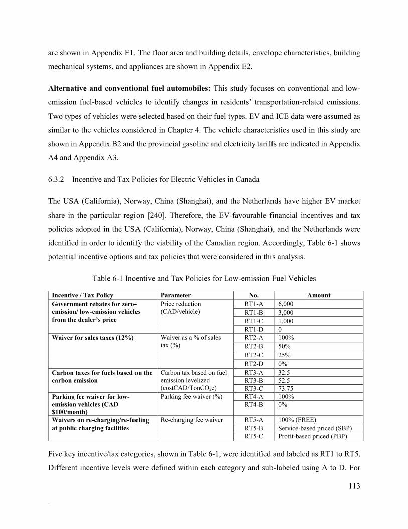
113

.

are shown in Appendix E1. The floor area and building details, envelope characteristics, building

mechanical systems, and appliances are shown in Appendix E2.

Alternative and conventional fuel automobiles: This study focuses on conventional and low-

emission fuel-based vehicles to identify changes in residents’ transportation-related emissions.

Two types of vehicles were selected based on their fuel types. EV and ICE data were assumed as

similar to the vehicles considered in Chapter 4. The vehicle characteristics used in this study are

shown in Appendix B2 and the provincial gasoline and electricity tariffs are indicated in Appendix

A4 and Appendix A3.

6.3.2 Incentive and Tax Policies for Electric Vehicles in Canada

The USA (California), Norway, China (Shanghai), and the Netherlands have higher EV market

share in the particular region [240]. Therefore, the EV-favourable financial incentives and tax

policies adopted in the USA (California), Norway, China (Shanghai), and the Netherlands were

identified in order to identify the viability of the Canadian region. Accordingly, Table 6-1 shows

potential incentive options and tax policies that were considered in this analysis.

Table 6-1 Incentive and Tax Policies for Low-emission Fuel Vehicles

Incentive / Tax Policy Parameter No. Amount

Government rebates for zero-

emission/ low-emission vehicles

from the dealer’s price

Price reduction

(CAD/vehicle)

RT1-A 6,000

RT1-B 3,000

RT1-C 1,000

RT1-D 0

Waiver for sales taxes (12%) Waiver as a % of sales

tax (%)

RT2-A 100%

RT2-B 50%

RT2-C 25%

RT2-D 0%

Carbon taxes for fuels based on the

carbon emission

Carbon tax based on fuel

emission levelized

(costCAD/TonCO2e)

RT3-A 32.5

RT3-B 52.5

RT3-C 73.75

Parking fee waiver for low-

emission vehicles (CAD

$100/month)

Parking fee waiver (%) RT4-A 100%

RT4-B 0%

Waivers on re-charging/re-fueling

at public charging facilities

Re-charging fee waiver RT5-A 100% (FREE)

RT5-B Service-based priced (SBP)

RT5-C Profit-based priced (PBP)

Five key incentive/tax categories, shown in Table 6-1, were identified and labeled as RT1 to RT5.

Different incentive levels were defined within each category and sub-labeled using A to D. For

114

.

example, “Waiver for Sales Tax” was identified as a key incentive for electric vehicles and labeled

as RT2. The tax waiver can be a “Full waiver” (100%), labeled as RT2-A; or a “half waiver”

(50%), labeled as RT2-B, and so on. Accordingly, 1,215 incentive schemes (combinations) were

identified for an EV-based transport system using the individual incentive options given in Table

6-1. The linear programming graphical method was used to identify the most desirable incentive

policy for each province.

6.3.3 Local Building Upgrades and Retrofit Options

The primary upgrades /retrofit options were identified from Okanagan builders and developers for

local single-detached households. Table 6-2 shows the aforementioned upgrade/retrofit options

that represent the above major components.

Table 6-2 Energy Retrofits for Single Detached Households

Retrofit

No.

Category Retrofitting

component

Retrofit

RB1

Energy-efficient building

envelope (enhance

insulation and enhance U-

value of windows)

(Additional Investment:

CAD16,932)

Foundation ICF blocks, 6” RCA reinforced, R-14 insulation, 2”

Styrofoam

Exterior wall

(Section 1)

3/8” EPS Styrofoam, 2”×6” wood studs @ 24” OC,

3/8” OSB sheeting, R-20 insulation, ½” drywall

Ground floor Engineered I joist 11 7/8” @ 19.2” OC, ¾” plywood,

R-14 insulation

Ceiling R-20 batt, R-50 blown-in ceiling, ½” drywall

Windows Vinyl triple glazed windows c/w 366 lowE Air

Tightness: 0.2 L/s.m2

RB2

Appliances (Additional

Investment: CAD2,535)

Heat recovery

system

ECM variable-speed blower

Stove and oven Energy Star rated double ovens (Avg: 450kWh/year,

Max: 615kWh)

Hot water

system

Energy star rated heat recovery electric hot water tank

2EF (Hot water temperature: 1310F)

RB3

Effective lighting (Ex:

LED and CFL)


CAD1,000)

Lighting

(interior)

More than 75% LED or CFL

RB4

Fuel switching to greener

HVAC systems to reduce

potential emissions (e.g.,

geo exchange-based

HVAC with multi-zoning)


CAD8,370)

Space heating

system

Ground heat source pump 4COP & Energy Star rated

electric fireplace 100% SS

HVAC

controller

SMART HVAC controller with multi-zoning

Space cooling

system

Ground heat source pump 5.6COP

RB5

Alternative in-situ green

energy production

(CAD9,385)

Solar (PV) 140 ft2 solar array, 150 Azimuth, 14.2% module

efficiency and 90% inverter efficiency

115

.

The specifications of the conventional household are shown in Appendix E3.

Initially, the energy model of the base case building was modeled using HOT2000 V11.3b90

developed by CANMET Energy Technology Center (CECT). The model was further modified

with multiple simulations considering all possible retrofit combinations (32 retrofit combinations),

and the resultant energy consumptions were obtained and recorded for all provinces. The

provincial weather profiles were obtained from CECT weather data libraries. The results generated

from the energy simulations were transferred to HIPT with the specification of each combination.

The utility tariff data used in this study are indicated in Appendix A5. Moreover, the current

incentive programs for SFDH upgrades available in Canadian provinces are shown in Table 6-3.

Provincial electricity GHG emission factors were obtained from Perera et al. (2017) [70]. Natural

gas cradle-to-grave emission factors were obtained as 49.87 kgCO2e/GJ Natural Gas [241].

Moreover, the HIPT was further extended with the TOPSIS method, which was used to rank all

32 building upgrade /retrofit options for all seven provinces.

116

.

Table 6-3 Provincial Incentive Schemes for Residential Buildings

Source: On-line databases of provincial utility providers and government institutions (Accessed in November 2017)

Quebec (QC) Ontario

(ON) British

Columbia (BC) Alberta (AB) Saskatchewa

n (SK) Manitoba

(MN) Nova Scotia

(NS)

Base house H2M (House with retrofits) H2D H2M H2D H2M H2D H2M H2D H2M H2D H2M H2D H2M H2D H2M

8” reinforced concrete, R-22

insulation

ICF blocks, 6” RCA reinforced, R-

14 insulation, 2”styroform

0 0 625 1250 0 0 132 132 0 0

0 0 0 5000

2”×6” wood studs @ 24” OC, 3/8” OSB sheeting, R-20 insulation, ½”

drywall

3/8” EPS Styrofoam, 2”×6” wood

studs @ 24” OC, 3/8” OSB

sheeting, R-20 insulation, ½” drywall

0 0 1875 1875 0 0 129

8 1298 0 0

Engineered I joist 11 7/8” @ 19.2”

OC, ¾” plywood, R-11 insulation

Engineered I joist 11 7/8” @ 19.2”

OC, ¾” plywood, R-14 insulation 0 0 190 190 0 0 0 0 0 0

R-22 Batt, R-40 blown in celling, ½” drywall

R-20 batt, R-50 blown in celling, ½” drywall

0 0 500 750 0 0 788 788 0 0

Vinyl double-glazed windows c/w

180 lowE Air Tightness: 0.2 L/s.m2

Vinyl triple-glazed windows c/w

366 lowE Air Tightness: 0.2 L/s.m2

0 0 0 0 0 0 0 500 0 0

Single stage PSC blower ECM variable speed blower 0 0 375 375 0 0 0 0 0 0 150 150 0 0

Standard Refrigerator Standard Refrigerator 0 0 0 0 100 100 100 100 0 0 0 0 0 0

Standard energy star cloth dryer Standard energy star cloth dryer 0 0 0 0 100 100 100 100 0 0 0 0 0 0

Standard Energy Star rated Cooker and oven (565kWh/year)

Energy Star rated Double ovens

(Avg: 450Wh/year, Max:

615kWh)

0 0 0 0 0 0 0 0 0 0 0 0 0 0

Energy star rated natural gas hot water tank 1EF (Hot water

temperature: 1310F) (60Gal)

Energy star rated heat recovery electric hot water tank 2EF (Hot

water temperature: 1310F)

0 0 375 375 1000 1000 945 0 0 0 0 0 0 0

25%-75% LED or CFL More than 75% LED or CFL 0 0 0 0 0 0 0 0 0 0 0 0 0 0

Energy star rated duel fuel (Natural

Gas & electric) EF - 92.1%, 56000 BTU/hr, switching temperature

350F & Natural gas fireplace 2kW,

6824.28 BTU/hr 30% SS

Ground heat source pump 4COP & Energy Star rated electric fireplace

100% SS

0 2800 625 4375 2000 0 0 0 0 0 0 0 0 0

SMART HVAC controller SMART HVAC controller with

multi-zoning

25 225 0 0 0 0 100 100 0 0 0 0 0 0

Energy star rated central split

system, (electric), 14SEER Ground heat source pump 5.6COP

0 0 250 250 0 0 0 0 0 0 0 0 0 0

Not available 140 ft2 Solar array, 150 Azimuth, 14.2% module efficiency & 90%

inverter efficiency

0 0 0 0 0 0 0 2607 0 0 0 5000 0 0

117

.

6.4 Results and Discussion

The results obtained from the transport incentive and building retrofit assessment are discussed in

this section.

6.4.1 Regional Retrofit or Upgrade Selection for Single Detached Houses

All the retrofit options and their combinations (32 combinations) were assessed and ranked to

obtain the best retrofit option based on regional characteristics. As an example, the results obtained

for BC, Canada are shown in Figure 6-2.

Figure 6-2 Building Level GHG Emissions and LCC vs. Retrofitting Investment for BC, Canada

According to Figure 6-2, the annual GHG emissions and building life cycle costs to the consumer

are indicated against the additional retrofitting investment per residential building. The trend

shows that annual GHG emissions of residential buildings decrease with increasing retrofit

investments. However, the annualized consumer cost also increases with additional retrofitting

investments due to resultant mortgage payments of premium upgrade costs. Therefore, in this

section, the environment and economic parameters were given equal weights. Accordingly, capital

investment and annualized consumer cost were each assigned a weight of 0.25 and GHG emissions

An

nu

al G

HG

em

issi

on

s (k

gC

O2eq

/yea

r)

118

.

were assigned a weight of 0.5. Based on the TOPSIS results, the distance to the ideal solution was

calculated. Accordingly, the best retrofit option for each province is shown in Table 6-4.

Table 6-4 Regional Retrofit Selection for SFDHs

Most desirable retrofit combination based on regional characteristics

Quebec

(RQC)

Ontario (RON) Alberta (RAB) British

Columbia (RBC)

Saskatchewan

(RSK)

Manitoba (RMN) Nova Scotia (RNS)

RB2+RB4 RB3 RB3 RB4 RB3 RB2+RB4 RB3

Parameter values for the house with retrofits

RQK RON RAB RBC RSK RMN RNS

HHE

H 58.11 1,626.63 1,2476.25 152.48 11,133.80 87.02 12,436.25

HHC

H 26,716.63 28,401.52 26,126.33 27,297.00 28,598.36 26,264.29 29,802.53

GCCH 3,025.00 9,440.00 5,623.98 3,200.00 500.00 5,150.00 5,000.00

Parameter values for house without (w/o) retrofits

W/O-RQK W/O-RON W/O-RAB W/O- RBC W/O-RSK W/O-RMN W/O-RNS HHE

H 168.13 1,657.96 1,2695.78 199.43 11,358.06 234.23 12,603.43

HHC

H 27,255.49 28,375.56 26,073.52 27,319.01 28,575.40 27,013.01 29,770.26

GCCH 25.00 4,815.00 3,461.74 1,200.00 0.00 150.00 0.00

According to Table 6-4, RB2 (high energy-efficient appliances) and RB4 (fuel switching to

greener HVAC systems) are affordable and the most effective retrofitting methods for the

provinces with low-emission electricity grid. Energy-efficient equipment is capable of reducing

electricity consumption in the house, and greener HVAC systems (e.g. ground source heat pump)

can reduce the use of natural gas consumption for space heating and cooling. Traditional homes in

provinces with high-emission electricity grids (fossil and coal power source electricity) can reduce

their electricity usage by promoting energy-efficient lighting systems. Heat-source pump-based

HVAC systems are not desirable for provinces with high-emission electricity grids due to the

extensive electricity consumption of the heat pump. Hence, energy-efficient natural gas HVAC

systems can be more productive and affordable. Additional wall and roof insulation and multiple-

pane windows (RB1) will enhance energy efficiency in all provinces. However, according to the

analysis, the capital retrofitting investment for additional insulation would be significant.

119

.

6.4.2 Best Incentive and Tax Policies for Electric Vehicles

The life cycle cost (LCC) of the EV was assessed and arranged in ascending order to select the

best incentive scheme based on regional characteristics. Vehicle lifespan was assumed as five

years [70]. Figure 6-3 shows the LCC gap between EV and ICE vehicles in BC for different

incentive schemes (LCC gap between EV and ICE vehicles for different incentives in all other

provinces are shown in Annex E). The majority of those schemes show more significant LCC

reductions to the consumer. However, those LCC savings will directly or indirectly affect

provincial and federal governments as a loss of income or as an additional expenditure. Therefore,

the selection criteria can be changed with the decision maker’s opinions and expert judgment by

incorporating a premium cost amount based on the potential buyers’ willingness to pay for electric

vehicles. However, in this work, it was assumed that potential buyers would pay no premium for

electric vehicles. Hence, the resultant incentive schemes were selected where the LCC of potential

EVs should be equal to or less than the LCC of ICEs.

Figure 6-3 Difference of LCC of EV with LCC of ICEV vs. Potential Incentives for BC, Canada

According to Figure 6-3, multiple results (points) that match the selection criteria were indicated

from the analysis. However, the combinations of individual retrofit types were selected to find the

provincial economic and environmental impacts of improving low-emission vehicle demands.

RT1, RT2, RT4, and RT5 reduce consumer cost and RT3 reduces the gap of the costs between

conventional and low-emission vehicles. Moreover, RT3 increases the operating cost of both

conventional and low-emission vehicles, which discourages private automobile usage in the long

120

.

run. Table 6-5 shows the incentive and tax policies selected for each province based on regional

characteristics.

Table 6-5 Province-based Incentive and Tax Policies

Quebec Ontario Alberta British

Columbi

a

Saskatchewa

n

Manitoba Nova Scotia

Desirable

policy

combination

RT1D+RT

2C+RT3C+

RT4B+RT5

B

RT1C+RT2B

+RT3B+RT4

B+RT5B

RT1D+RT2B

+RT3B+RT4

B+RT5B

RT1D+RT2

C+

+RT4B+RT

5B

RT1B+RT2B+RT

3B+RT4B+RT5B

RT1C+RT2D

+RT4B+RT5

B

RT1A+RT2D+R

T3C+RT4B+RT5

C

Incentive

category

Scheme

RT1 ($/vehicle)

0 1,000 0 0 3,000 1,000 6,000

RT2 25% 50% 50% 25% 50% 0% 0%

RT3 ($/TonCO2e)

73.75 52.50 52.50 0 52.50 0 73.75

RT4 50% 50% 50% 50% 50% 50% 50%

RT5 SBP SBP SBP SBP SBP SBP PBP

EV with

Incentives

EVQC EVON EVAB EVBC EVSK EVMN EVNS

HHEV 826.95 1,396.72 5,827.60 859.38 5,399.20 830.01 5,093.20 HHCV 11,466.9

0

11,447.56 11,423.05 11,672.16 11,447.50 11,510.96 11,409.96

GCCV 1,527.75 3,282.98 860.29 1,535.07 4,346.27 1,854.46 4,951.61

ICE w/o

incentives

ICEQK ICEON ICEAB ICEBC ICESK ICEMN ICENS

HHEV 2,980.64 2,980.64 2,980.64 2,980.64 2,980.64 2,980.64 2,980.64 HHCV 11,473.5

7

11,448.62 11,440.58 11,674.81 11,476.20 11,530.58 11,410.25

GCCV -158.93 -112.87 -112.87 0.00 -112.87 0.00 -158.93

6.4.3 Decision Making for Government Incentive Investment

The results shown in Table 6-4 and Table 6-5 are used to identify the eco-efficiency of transport

and residential building incentive programs in each province. Accordingly, this work identified

the amount of GHG emission reduction per dollar spent by the government for building and

transport sector incentives. Equation 5 was used to obtain the eco-efficiency ratio for these cases.

The eco-efficiency ratios obtained for each province are shown in Figure 6-4. Accordingly, the

incentives given for building retrofits in Nova Scotia, Alberta, and Saskatchewan show positive

GHG reductions, whereas the incentives given for EVs result in negative GHG reductions.

Accordingly, in these provinces, electrified transportation may increase life cycle emissions in the

121

.

long run. Therefore, the provinces with high-emission electricity grids can focus on incentive

schemes for building retrofits.

Figure 6-4 Compare the Eco-efficiencies of Electrified Transportation and Building Retrofitting

Figure 6-4 shows lower emission reductions for building retrofits compared to the incentives given

for electrified transportation. Therefore, provinces with low-emission electricity grids, such as

British Columbia, Manitoba, and Quebec, can focus on incentives and tax rewards for EVs and

EV infrastructure development projects. Proper incentive schemes for EVs will result in these

provinces achieving their GHG targets faster.

6.4.4 Consumer-centric Decision-making

The provincial-based annual household emissions for different scenarios (HHESiAnnualized) are

indicated in Figure 6-5. Accordingly, provinces that have low-emission electricity, like British

Columbia, Manitoba and Quebec, show significantly lower emissions in both scenario 1 and

scenario 3. Accordingly, electricity-operated vehicles and residential buildings have high potential

in these provinces due to the low-emission hydroelectric grid. Nova Scotia, Saskatchewan, and

Alberta show comparatively high emissions in all scenarios. However, scenario 4 shows slightly

lower emissions than other scenarios. Therefore, the provinces that have high emission electricity

can focus on retrofitting residential buildings instead of electric mobility. Conventional fuel

vehicles with greater fuel efficiencies might reduce GHG emissions in the short run. Nevertheless,

-15.0

-10.0

-5.0

0.0

5.0

10.0Quebec

Ontario

Alberta

British ColumbiaSaskatchewan

Manitoba

Nova Scotia

Electrified transportation eco-efficiency ration (kgCO2 reduction /$ invested)

Residential building retrofitting(kgCO2 reduction / $ invested)

122

.

active transportation systems such as walking, cycling, and low-emission public transit systems

would be the best options in the long run.

Figure 6-5 Household GHG Emissions and Consumer Annual Cost Comparison

In addition to GHG emissions, consumer operational cost is also essential in describing the

practicality of these greener interventions. Therefore, the annualized household cost for different

scenarios (HHCSiAnnualized) was also analyzed and shown in Figure 6-5. Consumer costs for the four

scenarios in all provinces do not show much difference, because the transport incentives have

made the cost of EVs approximately similar to the cost of conventional vehicles. However, there

is a minor cost difference among scenarios, which is mostly based on the operational cost of

residential buildings due to climate actions of different provinces. However, the eco-efficiency

method was used to analyze these scenarios further.

The GHG emission reduction requirements to achieve local and provincial targets and the

consumer cost premiums for reduced GHG levels were considered in the HEEI analysis. The

results obtained for HHC and HHE are provided in Appendix E4 for different scenarios. The

provincial comparison for HEEI is shown in Figure 6-6. A lower HEEI represents an increase in

GHG reduction for each dollar spent. According to Figure 6-6, Manitoba, Ontario, Quebec, and

British Columbia show a similar pattern in all scenarios, where scenario 3 and scenario 1 have

significantly lower HEEIs than the other scenarios. Scenario 3 shows the lowest HEEI, which

contains H2M with EVs. The premium price pays for the H2M and EVs has reduced GHG

123

.

Figure 6-6 Province-wise Household Eco-efficiency Index (HEEI)

emissions drastically. Accordingly, the government can promote both H2M and EVs by giving

more tax rewards to users.

Additionally, improving availability and accessibility to infrastructure for electric mobility will

reduce range anxiety6, which leads to increases in electric mobility in these provinces. Therefore,

local/provincial authorities with low-emission electricity grid can quickly achieve their long-term

and short-term GHG reduction targets due to increasing EV demands. Other provinces, like Nova

Scotia, Saskatchewan, and Alberta, do not show significant differences in HEEI in all scenarios

6For widespread adoption of AFVs, the range can be considered as a physiological barrier [12]. Limitations in available

locations of alternative fuel infrastructure and the lower range of vehicle cause a psychological effect on consumers

which is known as “range anxiety” [12]. Range anxiety makes potential consumers to decide against the use of AFVs.

124

.

and thus can focus on low-emission based retrofits for residences, such as LED lighting, energy-

efficient appliances, and insulation for building envelope. The provincial governments of the

aforementioned provinces need to focus their incentives more on residential building retrofit

improvements to achieve their provincial GHG targets.

The outlined analysis demonstrates that provinces with low-emission electricity, like British

Columbia, Manitoba, and Quebec, need to invest in electrified light-duty vehicles to reduce GHG

emissions. The provincial government of these provinces can provide incentives and invest in

charging-infrastructure facilities to enhance EV penetration. As the second priority, the above

provinces can develop an incentive scheme for alternative-fuel HVAC systems to reduce GHG

emissions further, which reduces the potential fossil fuel (natural gas) consumption for space

heating and water heating. Hence, the low-emission and low-cost alternative fuels or fuel hybrids

such as electricity/geo-exchange, etc. were used to replace fossil fuel-based appliances. As the

third priority, the aforementioned provinces can award rebates for energy-efficient appliances and

LED lighting. Finally, incentives can be granted for additional building envelope insulation

upgrades or retrofits.

Alberta, Nova Scotia, and Saskatchewan have high-emission electricity grids. Therefore, the use

of electricity should be minimized in these provinces, and alternative fuels such as natural gas and

hydrogen can be used for household activities. Hydrogen-based vehicles can be a better option for

the above provinces. However, hydrogen vehicles were not considered in this analysis due to the

lack of available data. Moreover, provincial incentives can be developed to increase the use of

energy-efficient appliances, LED lighting, and energy-efficient natural gas space heating and water

heating systems.

6.5 Summary

Premium investment costs and higher payback periods are the fundamental limitations of electric

vehicle transportation and energy-efficient building upgrades. Various incentive policies are used

to share the total impacts of investment cost among multiple stakeholders and encourage

consumers to switch to greener initiatives. Accordingly, local, provincial, and federal governments

are providing incentives for different sectors without assessing the overall household impacts

125

.

scientifically. Direct and indirect incentives that are provided for energy retrofits of residential

buildings and greener transportation can be considered as the domestic sector incentivizes to

reduce potential GHG emissions. Prioritizing interventions within the household cluster and

providing the right amount of incentives to the most desirable interventions is vital to maximizing

the effectiveness and efficiency of governments’ contribution, which will ensure maximum

consumer engagement to achieve government GHG targets faster.

This work focused on the emissions and cost of residential buildings and the transport activities

within the household cluster. A comprehensive literature review was conducted, and the life cycle

costs and impact data for EVs were collected from prior phases. Subsequently, a decision support

tool was prepared for all combinations of retrofits and incentive schemes. The MCDM-based

framework was used with a scenario-based decision-making approach. The potential economic

and environmental impacts of low-emission intervention investments were also discussed for the

considered scenarios. Government-centric and consumer-centric investment priorities for each

province were identified.

The results of this chapter indicate that the “Moderate future” incentive scenario, which consists

of electrified residential buildings with EVs are more desirable for provinces like Manitoba, British

Columbia, Ontario, and Quebec. These interventions would reduce building and transport GHG

emissions in the long run. The proposed incentive schemes for EVs can be comprised of purchasing

rebates and sales tax waivers for EVs, EV parking fee waivers, and government-subsidized

recharging costs. It was recommended to implement carbon tax policies to discourage fossil fuel

vehicles and reduce passive transportation in the future. The “Beyond Conventional” incentive

scenario, consisting of houses with retrofits with conventional fossil fuel vehicles is more desirable

for provinces like Saskatchewan, Alberta, and Nova Scotia. Hence, their incentive policies can be

focused on incentives for residential building retrofits to achieve their GHG targets faster.

Incentive schemes can be developed on energy-efficient natural gas-based HVAC systems and

energy-efficient appliances. Moreover, the additional income from carbon taxes can be used as

incentives for infrastructure investments and to develop recharging infrastructure for EVs. Hence,

the overall economic impacts to the government due to electrified transportation can be reduced,

which may lead to achieving provincial GHG targets faster than usual.

126

Chapter 7 Project Delivery Method Selection for Electric Vehicle Refuelling

Infrastructure Deployment

A version of this chapter is under preparation for a peer-reviewed journal paper, as an article titled

“Project delivery method selection for electric vehicle refuelling infrastructure deployment: A

fuzzy-based approach” that will be submitted to the Journal of Cleaner Production in July 2020.

7.1 Background

The life cycle of the electric vehicle recharging infrastructure project can be described using key

project phases: construction, operation, maintenance, and end-of-life [175][176]. The construction

phase has a greater investment, whereas the operational phase generates revenue [242]. The

success of EV-RI projects depends on acquiring the anticipated demands; identifying potential

risks; deploying risk sharing; allocation, and mitigation strategies; and maintaining the anticipated

project performance [157]. According to the Rogers diffusion model, EV recharging demands and

associated economic risks are dynamic in nature and vary with the maturity level of the EV market.

Project Delivery Methods (PDMs) are used to share project risks among project stakeholders and

ensure minimal risk to concerned parties [54]. In addition to the risk, properly selected PDMs

allows projects to obtain third-party assistance in relation to technical know-how, resources, design

and management standards, and other project-related benefits while ensuring possible benefits to

all stakeholders [162][243]. Lower paybacks, unnecessary responsibility allocation, and adverse

opportunity costs are possible disadvantages of selecting less suitable PDMs [243]. Moreover,

PDMs can be used to create professional relationships among project stakeholders such as project

owners, designers, builders, and managers to pursue and complete a project successfully while

utilizing team synergies [244][245].

The current knowledge on existing projects shows that project owners or project managers are the

key decision-makers in selecting the PDM method [243][245]. Concerning innovative and novel

projects, project owners, and project managers might not have the necessary experience and

expertise to select the most suitable PDM, so key stakeholder perception also enhances the

effectiveness of the above decisions [243]. Hence, PDM selection for public EV-RI development

127

projects requires project stakeholder opinion to overcome possible deployment challenges such as

defining needs, acquiring funding, and dealing with project-related risks, design, and construction

issues [246].

A comprehensive literature review revealed that multiple researchers published articles on PDM

selection for construction projects [162][53]. However, most of those researchers overlooked PDM

selection complications that arise with novel and innovative projects and the involvement of key

stakeholders [55][247]. By integrating stakeholder opinion on PDM selection, the synergies that

are formed by project stakeholders can be used to overcome project limitations such as lack of

technical know-how and experience with innovative and novel projects at their initial stages.

Moreover, the financial risks of those projects due to demand uncertainties and other potential

technical uncertainties can be managed collectively, and the risk can be minimized for project

decision-makers. A compensatory MCDM approach will strengthen the collective decision

making and provide a scientific platform.

This chapter presents a framework to select the stakeholder expertise-based PDM method for

innovative and novel projects. A fuzzy multi-attribute decision-making approach was introduced

to rank alternative PDM methods to identify the most desirable PDM method for long-range EV-

RI deployment projects in urban centers. The developed methodology was applied to the case

study in Chapter 5 to identify possible PDMs for multi-period EV-RI planning projects for

Kelowna, BC.

7.2 Methodology for PDM Selection Framework

The methodology of this work initiated with a comprehensive literature review and expert

interviews on current PDM selection strategies for construction projects. Figure 7-1 shows the

method adopted to develop the PDM selection framework considering the stochastic and temporal

variation of the estimated EV demands.

128

Figure 7-1 PDM Selection Methodology for EV-RIs

The phases of the PDM selection framework are further explained below.

Phase 1: Identification of PDM selection attributes

The database related to project delivery methods (PDMs), factors, and different characteristics of

mostly available PDMs were collected from recently published literature. Recent peer-reviewed

journal articles, conference proceedings, and institutional reports were used to collect the

background data related to infrastructure management and PDMs for infrastructure development

129

projects. PDMs for infrastructure projects, PDM selection factors, infrastructure risk management,

and infrastructure cost-sharing were used as keywords for the literature review. Table 7-1 shows

prominent attributes that help determine the most desirable PDM for small-scale and medium-

scale infrastructure development projects such as EV-RI facilities. These attributes were selected

using existing literature and validated by subject experts.

Table 7-1 PDM Selection Factors

Section

Attributes Selection

Attribute

No.

Description Ref.

Project

characteristics

Scope definition SA 1

Maximize the importance of having a pre-defined

scope baseline for the project (Not an agile type of

a project)

[162]

Project schedule SA 2 Maximize the importance of having very accurate

and tight project schedules and baselines.

[162]

[161]

Contract

Strategy SA 3

Minimize the cost uncertainties due to not having

cost baseline and contract strategy (High-cost

uncertainties in measure and pay, cost-plus, etc.)

[162]

Complexity SA 4

Maximize the external expertise for complex

projects for identifying the technical-know-how

requirement

[162]

[163]

[161]

Owners pre-

requests

Constructability

studies SA 5

Maximize the importance of the constructability

studies before the project initialization

[162]

Value

engineering

studies

SA 6

Maximize the importance of the involving value

engineering processers during the project to

enhance the project efficiency

[162]

Contract

packaging SA 7

Maximize the importance of creating work

packages and award contracts accordingly.

[162]

Contract

awarding criteria SA 8

Maximize the importance of having a systematic

contract awarding criteria, which will consider cost,

quality, and previous experiences for the selections.

[162]

Cost Sharing SA 9

Maximize the importance of cost-sharing or

additional funding due to the expensiveness and

lower pay-back of the project

[162]

[161]

Owners

preferences

Responsibility SA 10 Minimize the owners’ responsibilities to obtain

minimal risks and responsibilities

[161]

Design control SA 11 Maximize the importance of having design control

to the owner at the initiation and during the project.

[163]

[161]

Involvement

after awarding SA 12

Minimizing the owners’ involvement during the

project and keep minimal disturbance to the owner

[163]

Risk

Change orders SA 13 Minimize the possibilities of initiating a high

amount of change orders during the project.

[162]

Risk-sharing SA 14

Maximize the importance of the risk-sharing or risk

allocating ability from the owner to a third party in

a high-risk project.

[162]

Quality

Quality control

and quality

assurance

SA 15

Maximize the importance of having a specific

avenue to conduct third party quality control and

quality assurance.

[162]

130

These factors were used to develop the decision matrix for alternative PDMs.

Phase 2: Determine the importance of PDMs and develop a decision matrix

The literature revealed that there are multiple PDMs for different infrastructure development

projects. The key PDMs can be categorized as Traditional; Partnership; or Collaborative [159].

Literature-based details on the selected PDMs are shown in Table 3-6. Six PDMs were considered

to develop the decision matrix: 1) Design-Bid-Build (DBB) (Traditional method); 2) Design-Build

(DB) (Collaborative method); 3) Construction Management at Risk (CM) (Collaborative method);

4) Design-Built-Operate and Transfer (DBOT) (Partnership method); 5) Public-private partnership

(PPP) (Partnership method); and 6) Integrated Project Delivery (IPD) (Collaborative method). The

studies conducted by Oyetunji A. A. and Anderson S. D (2006) and Mostafavi A. and Karamouz

M. (2010) were used to identify the relative importance of each factor for the above considered

PDMs [157]. The following linguistics terms were used to indicate the relative importance of the

attributes for each PDM:

‘Not Applicable’ was used when the attribute is not applicable to be considered for the EV

maturity level

‘Equally Important’ was used when the attribute is applicable but have no considerable

impact on the selection of PDM.

‘Moderately Important’ was used when the attribute is applicable and has considerable

impact on the selection of a PDM.

‘Strong Important’ was used when the attribute is applicable and has a significant impact

on the selection of a PDM.

‘Very Strong Important’ was used when the attribute is applicable and has a very strong


‘Extremely Important’ was used when the attribute is applicable and has an extremely high


Table 7-2 shows the relevant attribute values based on the PDM.

131

Table 7-2 Decision Matrix for the Proposed PDM Selection Approach

Attribute

No.

Decision

Type Linguistic Terms

MAX MIN DBB DB CM DBOT PPP IPD

SA 1 1 0 Equal

Important

Extremely

strong

Equal

Important

Strong

important

Extremely

strong

Extremely

strong

SA 2 1 0 Equal

Important

Equal

Important

V. Strong

important

Equal

Important

Strong

important

Equal

Important

SA 3 0 1 Equal

Important

Equal

Important

Extremely

strong

Equal

Important

Equal

Important

Strong

important

SA 4 1 0 Extremely

strong

Equal

Important

V. Strong

important

Strong

important

V. Strong

important

Extremely

strong

SA 5 1 0 Not

Applicable

Extremely

strong

Not

Applicable

Extremely

strong

Moderate

Important

V. Strong

important

SA 6 1 0 Not

Applicable

Extremely

strong

Not

Applicable

Extremely

strong

Moderate

Important

Extremely

strong

SA 7 1 0 Not

Applicable

Extremely

strong

Not

Applicable

Extremely

strong

Moderate

Important

V. Strong

important

SA 8 1 0 Equal

Important

Extremely

strong

Equal

Important

V. Strong

important

Strong

important

V. Strong

important

SA 9 1 0 Not

Applicable

Moderate

Important

Not

Applicable

Extremely

strong

Extremely

strong

Moderate

Important

SA 10 0 1 V. Strong

important

Extremely

strong

Equal

Important

Moderate

Important

Extremely

strong

Moderate

Important

SA 11 1 0 Extremely

strong

Equal

Important

Strong

important

Equal

Important

Strong

important

Moderate

Important

SA 12 0 1 Equal

Important

Extremely

strong

Equal

Important

V. Strong

important

Strong

important

Moderate

Important

SA 13 0 1 Extremely

strong

Equal

Important

Strong

important

Equal

Important

Strong

important

Moderate

Important

SA 14 1 0 Equal

Important

Moderate

Important

Strong

important

Extremely

strong

Extremely

strong

Moderate

Important

SA 15 1 0 Extremely

strong

Moderate

Important

V. Strong

important

Equal

Important

V. Strong

important

Extremely

strong

The attributes shown in Table 7-2 were converted to triangular-fuzzy numbers using the scale

shown in Table 7-3.

Table 7-3 Triangular-fuzzy Numbers used to Convert Attributes of Different PDMs

Linguistic Terms Triangular fuzzy numbers

Not Applicable (𝑎1, 𝑎1, 𝑎1)

Equal Important (𝑎1, 𝑎2, 𝑎3)

Moderately Important (𝑎2, 𝑎3, 𝑎4)

Strong Important (𝑎3, 𝑎4, 𝑎5)

Very Strong Important (𝑎4, 𝑎5, 𝑎6)

Extreme Important (𝑎5, 𝑎6, 𝑎6)

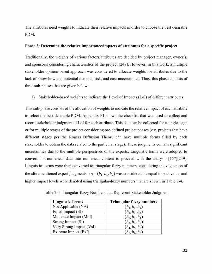
132

The attributes need weights to indicate their relative impacts in order to choose the best desirable

PDM.

Phase 3: Determine the relative importance/impacts of attributes for a specific project

Traditionally, the weights of various factors/attributes are decided by project manager, owner/s,

and sponsor/s considering characteristics of the project [248]. However, in this work, a multiple

stakeholder opinion-based approach was considered to allocate weights for attributes due to the

lack of know-how and potential demand, risk, and cost uncertainties. Thus, this phase consists of

three sub-phases that are given below.

1) Stakeholder-based weights to indicate the Level of Impacts (LoI) of different attributes

This sub-phase consists of the allocation of weights to indicate the relative impact of each attribute

to select the best desirable PDM. Appendix F1 shows the checklist that was used to collect and

record stakeholder judgment of LoI for each attribute. This data can be collected for a single stage

or for multiple stages of the project considering pre-defined project phases (e.g. projects that have

different stages per the Rogers Diffusion Theory can have multiple forms filled by each

stakeholder to obtain the data related to the particular stage). These judgments contain significant

uncertainties due to the multiple perspectives of the experts. Linguistic terms were adopted to

convert non-numerical data into numerical content to proceed with the analysis [157][249].

Linguistics terms were then converted to triangular-fuzzy numbers, considering the vagueness of

the aforementioned expert judgments. aEI = (𝑏1, 𝑏1, 𝑏2) was considered the equal impact value, and

higher impact levels were denoted using triangular-fuzzy numbers that are shown in Table 7-4.

Table 7-4 Triangular-fuzzy Numbers that Represent Stakeholder Judgment

Linguistic Terms Triangular fuzzy numbers

Not Applicable (NA) (𝑏1, 𝑏1, 𝑏1)

Equal Impact (EI) (𝑏1, 𝑏1, 𝑏2)

Moderate Impact (MoI) (𝑏2, 𝑏3, 𝑏4)

Strong Impact (SI) (𝑏3, 𝑏4, 𝑏5)

Very Strong Impact (VsI) (𝑏4, 𝑏5, 𝑏6)

Extreme Impact (ExI) (𝑏5, 𝑏6, 𝑏6)

133

Accordingly, each stakeholder was denoted by a weight based on the importance of their decision

to select the PDM. The weights of the ith attribute, which was denoted by the jth stakeholder, was

shown as lower bound (LB) value of “pij”, most likely (ML) value of “qij”, and upper bound (UB)

value of “rij” [249]. Accordingly, the triangular fuzzy membership value of the ith criteria denoted

by jth stakeholder was (pij, qij, rij). “Xij” was considered as the matrix of the weights of the ith

criteria denoted by the jth stakeholder and is expressed in Equation (42).

Equation 42

Generally, these decisions are based on personal opinion, skills, experiences, and other available

resources of the selected decision-makers [248]. Areas of expertise of experts’ are not uniform.

Some experts have more knowledge of some attributes where other experts might have a lack of

knowledge. Thus, the PDM selection approach needs to be able to integrate different expertise in

the decision-making process.

2) Evaluate stakeholder expertise and incorporate Level of Expertise (LoE) weights

The LoI of the above attributes was defined by decision-makers or subject experts based on their

experiences and expertise, which are typically a qualitative (non-numerical) judgment [248]. Thus,

linguistics terms were used to express the Level of Expertise (LoE) of the decision-makers to adjust

the relative importance of the considered attributes. CNE = (𝑐1, 𝑐1, 𝑐1) was considered no expertise

and CLE = (𝑐1, 𝑐1, 𝑐2) was considered low expertise. Accordingly, higher expertise levels were

denoted using fuzzy-triangular numbers, shown in Table 7-5 [157].

Xij =

(p11,q11,r11) (p12,q12,r12) … (p1j,q1j,r1j) … (p1n,q1n,r1n)

(p21,q21,r21) (p22,q22,r22) … (p2j,q2j,r2j) … (p2n,q2n,r2n)

...

...

...

...

(ai1,bi1,ci1) (ai2,bi2,ci2) … (aij,bij,cij) … (ain,bin,cin)

...

...

...

...

(am1,bm1,cm1) (am2,bm2,cm2) … (amj,bmj,cmj) … (amn,bmn,cmn)

134

Table 7-5 Triangular-fuzzy Numbers to Incorporate Stakeholder Expertise for Decision-making

Description Linguistic Term Triangular fuzzy numbers

Not an expert No Expertise (𝑐1, 𝑐1, 𝑐1)

Had some experience Low Expertise (𝑐1, 𝑐1, 𝑐2)

An expert, but currently not practicing Moderate Expertise (𝑐1, 𝑐2, 𝑐3)

An expert and working as a professional High Expertise (𝑐2, 𝑐3, 𝑐3)

3) Multi-attribute group decision-making approach (Compensatory method)

Generally, multi-stakeholder problems are solved using mathematical approaches that are used to

optimize the decisions of rational decision-makers. The Simple Additive Weighting method can

be used to score combined judgments [187][186]. This is a compromising method that permits

trade-offs between stakeholders [187]. Accordingly, the jth stakeholder’s expertise to decide the ith

criteria was given the weight of “Wij” considering other stakeholders. “W’ij” represents the fuzzy

weights given based on the relative importance of the jth stakeholder to decide ith criteria. The

weighted sum of each criterion was calculated, and the final weights were created to proceed with

further analysis [249]. Accordingly, the equations for the final attribute weights can be shown as

Equation (43).

Equation 43

Basic fuzzy arithmetic operations consisting of fuzzy addition, multiplication, and division (see

Section 3.8.2) were used to solve Equation (42). The fuzzy weights associated with the multiple

stakeholder perspectives were used to proceed with PDM selection for the considered EV-RI

deployment.

𝑫𝒊′ =

𝑾𝟏′ = ∑ (𝑾𝟏𝒋⨂𝑿𝟏𝒋

𝒏

𝒋=𝟏) ∑ 𝑾𝟏𝒋

𝒏

𝒋=𝟏⁄

𝑾𝟐′ = ∑ (𝑾𝟐𝒋⨂𝑿𝟐𝒋

𝒏

𝒋=𝟏) ∑ 𝑾𝟐𝒋

𝒏

𝒋=𝟏⁄

...

𝑾𝒊′ = ∑ (𝑾𝒊𝒋⨂𝑿𝒊𝒋

𝒏

𝒋=𝟏) ∑ 𝑾𝒊𝒋

𝒏

𝒋=𝟏⁄

…

𝑾𝒎′ = ∑ (𝑾𝒎𝒋⨂𝑿𝒎𝒋

𝒏

𝒋=𝟏) ∑ 𝑾𝒎𝒋

𝒏

𝒋=𝟏⁄

135

Phase 4: Select the most desirable PDM using F-TOPSIS

The weights obtained from phase 3 (from different sub-phases) were considered for this phase.

Each alternative method was simulated individually. Fuzzy weights given to the kth alternative

were normalized to obtain the fuzzy decision matrix, which is Ãik = [ãik]. The positive ideal criteria

is shown in Equation (44) and the negative ideal criteria is shown in Equation (45).

To the positive ideal;

Ã𝑖𝑘 = (𝑝𝑖𝑘 𝑟𝑘∗⁄ , 𝑞𝑖𝑘 𝑟𝑘

∗⁄ , 𝑟𝑖𝑘 𝑟𝑘∗⁄ ) 𝑎𝑛𝑑 𝑟𝑘

∗ = max𝑖

{𝑟𝑖𝑘} Equation 44

To the negative ideal;

Ã𝑖𝑘 = (𝑝𝑘− 𝑟𝑖𝑘⁄ , 𝑝𝑘

− 𝑞𝑖𝑘⁄ , 𝑝𝑘− 𝑟𝑖𝑘⁄ ) 𝑎𝑛𝑑 𝑝𝑘

− = min𝑖

{𝑝𝑖𝑘} Equation 45

The 𝐷𝑖′ weights were used to calculate the weighted normalized fuzzy decision matrix, which is

Ã’ik = [ã’ik]. Equation (46) shows the calculation of Ã’ik .

Ã𝑖𝑘′ = Ã𝑖𝑘 𝐷𝑖

′ Equation 46

Then the fuzzy positive ideal solution (PIS) (most desirable alternative) and the fuzzy negative

ideal solution (NIS) (worst case alternative) were obtained [197][249].

To the positive ideal;

𝐴∗ = (Ã1′∗ , Ã2

′∗, … … . , Ã𝐾′∗), 𝑤ℎ𝑒𝑟𝑒 Ã𝑘

′∗ = 𝑚𝑎𝑥𝑖

{Ã𝑖𝑘𝑈𝐿′ } Equation 47

To the negative ideal;

𝐴− = (Ã1′− , Ã2

′−, … … . , Ã𝐾′−), 𝑤ℎ𝑒𝑟𝑒 Ã𝑘

′− = 𝑚𝑖𝑛𝑖

{Ã𝑖𝑘𝐿𝐵′ } Equation 48

Accordingly, Equation (47) and Equation (48) were used to calculate fuzzy PIS and fuzzy NIS.

Equation (12) was used to calculate the distances between the PIS that denotes as 𝑑(Ã𝒊𝒌′ , Ã𝒌

′∗), and

136

NIS, which denotes as 𝑑(Ã𝒊𝒌′ , Ã𝒌

′−). Accordingly, the above-calculated distances, the cumulative

distances (𝑑𝑖∗) and (𝑑𝑖

−) were calculated using Equation (49) and Equation (50).

𝑑𝑖∗ = ∑ 𝑑(𝐾

𝑘=1 Ã𝑖𝑘′ , Ã𝑘

′∗) Equation 49

𝑑𝑖− = ∑ 𝑑(𝐾

𝑘=1 Ã𝑖𝑘′ , Ã𝑘

′−) Equation 50

The above distances were used to calculate the closeness coefficient (CCi) for each PDM as shown

in Equation (51).

𝐶𝐶𝑖 = 𝑑𝑖− (𝑑𝑖

−⁄ + 𝑑𝑖∗) Equation 51

The closeness coefficient was used to rank the considered PDMs based on project attribute values.

The PDM method with the highest closeness coefficient (CC) was chosen as the most desirable

and recommended project delivery method to proceed with the project. Other PDMs were ranked

according to the CC obtained from the above analysis. Then the applicability of the selected PDMs

was discussed with favourable and adverse impacts considering the sustainability of the transport

electrification in a given urban center.

7.3 PDM Selection Model Demonstration

The data obtained from Chapter 5 was used to demonstrate the proposed PDM selection model.

Accordingly, multi-period EV-RI deployment data for the Census Metropolitan Area of Kelowna

were taken as model inputs, which were organized into two product maturity stages.

7.3.1 EV-RI Deployment Stages for Multiple Periods

The theory of adoption and diffusion (Rogers model) [146] was used to explain the market growth

of EVs in the long run. Accordingly, five key product maturity stages can be considered in EV-RI

deployment to the business-as-usual stage: 1) Innovators; 2) Early adopters; 3) Early majority; 4)

Late majority; and 5) Laggards [50]. The innovation stage can be considered as the very early stage

of electric vehicle testing in which there is a lack of commercialized product at the local market

[250]. Hence, this work was started by early adopters and continue up to laggards. As mentioned

137

by Perera et al. (2020), the different EV-RIs were segregated by the different deployment stages,

shown in Figure 7-2.

Figure 7-2 Maturity Stage-wise EV-RI Deployment

However, the aforementioned stages were combined and considered as two stages, described

below, to reduce the complexity of the data collection and expert consultation.

1. The initial deployment stage: Early adopters and early majority stages were combined in

this stage. The infrastructure developed and invested in early stages of the product maturity

can be considered in this stage of the project, which consists of higher financial risk due to

limited public charging demands and longer payback, inadequate technical know-how due

to lack of local DC-FC recharging infrastructure construction experience, and a high

potential for significant design changes during the construction and operating periods.

Constructability analysis can be done at the pre-planning stage of the project. However, it

might be too early to conduct work packaging and value engineering, since the project

processers, durations, and costs have higher uncertainties due to lack of experience. The

possibility of having potential design changes, change orders, and baseline changes are

considerably greater at the early stages of product maturity.

2. The way forward to the business-as-usual stage: Late majority and laggards were combined

in this stage. These investments have comparatively lower risk and lower paybacks than

the previous stage. Furthermore, the technical know-how is higher, where the potential

demands and risks can be calculated more accurately using historical data obtained from

the earlier investments. Infrastructure developers can use the previous project cost, time,

and schedule data to ensure proper costing, scheduling, and operating of the infrastructure.

138

Potential change orders will be limited during the project life cycle, and the owners' control

after awarding the contract will be minimized. With time, the deployment process turns in

to a usual development task, where there are minimal financial and technical risks. The

project implementation, operation, and management process will be in-placed, and the

project can be done as work packages. Value chain optimization can be done to minimize

costs and obtain a competitive advantage by enhancing the value of the infrastructure

facilities. The payback periods should be significantly lower compared to the previous

stage.

7.3.2 Stakeholder Data Collection for the Case Demonstration

Potential project stakeholders and subject experts were consulted to acquire necessary data to

demonstrate the developed methodology for a medium-scale community in BC. The ethics

approval obtained for the MITACS Fortis Energy Chair Project was used to conduct the expert

consultation process. In this case study, the experts were categorized as: 1) Utility providers and

existing investors, and 2) Project manager and developers. Their expertise was collected using

focus group interviews. The experts who were interviewed are shown in Table 7-6. The collective

opinion of each expert category was recorded using several focus-group interviews that were

conducted with the aforementioned stakeholders/experts.

Table 7-6 Focus Group Interview-based Data Collection and Database Development

Stakeholder

Category

Knowledge Area Number of Experts

consulted

1

Investors and Owners: This category includes current

owners, investors, utility providers, EV-RI operators, and

EV-RI facility managers

4

2

Project Managers and builders: This category includes

building and infrastructure developers, Marketing managers,

technology managers, PMs, and other construction-related

decision-makers.

4

The different weights obtained from the aforementioned experts are shown in Table 7-7 for both

the first and second stages of the EV-RI deployment process.

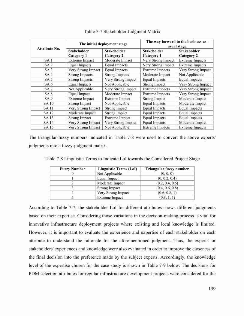
139

Table 7-7 Stakeholder Judgment Matrix

Attribute No.

The initial deployment stage The way forward to the business-as-

usual stage

Stakeholder

Category 1

Stakeholder

Category 2

Stakeholder

Category 1

Stakeholder

Category 2

SA 1 Extreme Impact Moderate Impact Very Strong Impact Extreme Impacts

SA 2 Equal Impacts Equal Impacts Very Strong Impact Extreme Impacts

SA 3 Very Strong Impact Equal Impacts Extreme Impacts Very Strong Impact

SA 4 Strong Impacts Strong Impacts Moderate Impact Not Applicable

SA 5 Strong Impacts Very Strong Impact Equal Impacts Equal Impacts

SA 6 Equal Impacts Not Applicable Strong Impact Very Strong Impact

SA 7 Not Applicable Very Strong Impact Extreme Impacts Very Strong Impact

SA 8 Equal Impact Moderate Impact Extreme Impacts Very Strong Impact

SA 9 Extreme Impact Extreme Impact Strong Impact Moderate Impact

SA 10 Strong Impact Not Applicable Equal Impacts Moderate Impact

SA 11 Very Strong Impact Strong Impact Equal Impacts Equal Impacts

SA 12 Moderate Impact Strong Impact Equal Impacts Equal Impacts

SA 13 Strong Impact Extreme Impact Equal Impacts Equal Impacts

SA 14 Very Strong Impact Very Strong Impact Equal Impacts Moderate Impact

SA 15 Very Strong Impact Not Applicable Extreme Impacts Extreme Impacts

The triangular-fuzzy numbers indicated in Table 7-8 were used to convert the above experts'

judgments into a fuzzy-judgment matrix.

Table 7-8 Linguistic Terms to Indicate LoI towards the Considered Project Stage

Fuzzy Number Linguistic Terms (LoI) Triangular fuzzy number

0 Not Applicable (0, 0, 0)

1 Equal Impact (0, 0.2, 0.4)

2 Moderate Impact (0.2, 0.4, 0.6)

3 Strong Impact (0.4, 0.6, 0.8)

4 Very Strong Impact (0.6, 0.8, 1)

5 Extreme Impact (0.8, 1, 1)

According to Table 7-7, the stakeholder LoI for different attributes shows different judgments

based on their expertise. Considering those variations in the decision-making process is vital for

innovative infrastructure deployment projects where existing and local knowledge is limited.

However, it is important to evaluate the experience and expertise of each stakeholder on each

attribute to understand the rationale for the aforementioned judgment. Thus, the experts' or

stakeholders' experiences and knowledge were also evaluated in order to improve the closeness of

the final decision into the preference made by the subject experts. Accordingly, the knowledge

level of the expertise chosen for the case study is shown in Table 7-9 below. The decisions for

PDM selection attributes for regular infrastructure development projects were considered for the

140

business-as-usual stage due to the lack of expertise on current mass scale EV-RI infrastructure

projects in the concerned community.

Table 7-9 Stakeholder Expertise in EV-RI Deployment and Conventional Infrastructure Projects

Attribute No.

Knowledge related to initial phases of

EV-RI planning and management

Knowledge related to conventional

infrastructure planning and

management

Stakeholder

Category 1

Stakeholder

Category 2

Stakeholder

Category 1

Stakeholder

Category 2

SA 1 Low Expertise High Expertise Low Expertise High Expertise



SA 4 High Expertise Low Expertise High Expertise Low Expertise

SA 5 High Expertise Low Expertise High Expertise Low Expertise

SA 6 Moderate Expertise Moderate Expertise Moderate Expertise High Expertise

SA 7 No Expertise No Expertise No Expertise High Expertise

SA 8 No Expertise Moderate Expertise Moderate Expertise Moderate Expertise

SA 9 High Expertise Moderate Expertise High Expertise Moderate Expertise


SA 11 High Expertise Low Expertise No Expertise High Expertise

SA 12 High Expertise Low Expertise No Expertise High Expertise

SA 13 Moderate Expertise High Expertise No Expertise High Expertise


SA 15 Moderate Expertise No Expertise No Expertise High Expertise

Table 7-9 shows that the experience and expertise of all stakeholders are not uniform. Although

the individual stakeholder expertise did not fulfill the full attribute list to finalize the best desirable

PDM for EV-RI projects, the combined expertise has covered the majority of those attributes.

Hence, combining multi-stakeholder judgments using compensatory methods will enhance the

applicability and reliability of the final PDM decision compared to the conventional individual

decision-making concepts.

The triangular-fuzzy numbers that are indicated in Table 7-10 were used to convert the linguistic

terms used in Table 7-9.

Table 7-10 Linguistics Terms to Indicate LoE of the Stakeholders on the Subjected Criteria [157]

Fuzzy Number Linguistic Terms (Expertise) Triangular fuzzy number

0 No expertise (0, 0, 0)

1 Low expertise (0, 0, 0.5)

2 Moderate expertise (0, 0.5, 1)

3 High expertise (0.5, 1, 1)

The LoE and LoI matrices are shown in Appendix F2 and Appendix F3, respectively.

141

7.3.3 PDM Decision Matrix for Ranking

Table 7-2 can be converted into a fuzzy matrix using triangular-fuzzy numbers. The triangular-

fuzzy numbers shown in Table 7-11 were used for the conversion.

Table 7-11 Linguistic Terms to Convert the Decision Matrix into Fuzzy Numbers [251]

Fuzzy Number Linguistic Terms (LoI) Triangular fuzzy number

0 Not Applicable (0, 0, 0)

1 Equal Important (0, 0.2, 0.4)

2 Moderate Important (0.2, 0.4, 0.6)

3 Strong Important (0.4, 0.6, 0.8)

4 Very Strong Important (0.6, 0.8, 1)

5 Extremely Strong (0.8, 1, 1)

The fuzzy decision matrix for alternative PDMs is shown in Appendix F4.

7.3.4 Multi-period and Multi-stakeholder-based Attribute Weights

As described in the methodology section 7.2, the compensatory weights were calculated using

Equation (43) for both stage one and two of EV-RI deployment projects. Those weights are given

in Appendix F5. The individual and compensatory weights for each attribute in stages one and two

were defuzzified to crisp numbers using the Center of Gravity method to show their relative

importance in the PDM selection process. Accordingly, Table 7-12 shows the impact of each

attribute that was used to select the best desirable PDM for EV-RI projects in different product

maturity stages.

142

Table 7-12 Final Weights of the Expert Data Collected as Inputs for the PDM Selection Tool

7.3.5 Ranking Alternative PDMs and PDM Selection

The F-TOPSIS method discussed in the methodology was used to select the best desirable PDM

method for different EV-RI deployment stages. Normalized attribute matrices, distances from the

negative and positive ideal solutions, and closeness coefficients for different PDM methods were

calculated. The final closeness coefficient of alternative PDM methods and rankings of those for

different life cycle stages are shown in Figure 7-3.

143

Figure 7-3 F-TOPSIS-based PDM Rankings for Multi-period EV-RI Deployment Projects

Figure 7-3 shows the rankings obtained using different stakeholder opinions and different

characteristics of EV-RI deployment stages.

Considering the initial EV-RI deployment stage, the resultant PDMs obtained from both individual

stakeholder opinions and their compensatory opinion resulted in a partnering PDM approach. The

analysis shows that the PPP method was proposed by stakeholder category 1: the potential and

current owners and investors based on their expertise. In addition, the DBOT method was proposed

by stakeholder category 2: PMs, builders, and developers based on their knowledge. As discussed

in section 7.3.4, lack of expertise is present in different stakeholder categories due to a lack of

project-related experiences. Thus, the compensatory method makes more sense to fulfill the

StakeholderCategory 1


CompensatoryWeight



CompensatoryWeight

The initial deployment stageThe way forward to the business-as-usual

stage

DBB 0.322 0.186 0.334 0.212 0.165 0.203

DB 0.464 0.553 0.429 0.625 0.680 0.637

CM 0.455 0.358 0.488 0.398 0.359 0.395

DBOT 0.629 0.796 0.648 0.636 0.658 0.643

PPP 0.801 0.730 0.787 0.702 0.690 0.708

IPD 0.682 0.653 0.650 0.731 0.757 0.755

0.000

0.100

0.200

0.300

0.400

0.500

0.600

0.700

0.800

0.900C

lose

nes

s C

oef

fici

ent

(CC

)EV-RI Initial Stages EV-RI Mature Stages

3

1

2

1

2

3

3

1

2

3

2

1

3

2

1

3

2

1

144

required expertise from multiple stakeholders and proceed with group-based decision-making. The

PPP method has resulted from the compensatory approach for the initial stages of EV-RI

deployment. Accordingly, the PPP can be considered the best desirable PDM for the EV-RI initial

development stages. Based on the EV-RI location-allocation and capacity enhancement plan for

Kelowna, BC, the potential fast public recharging facilities proposed for Glenmore, Springfield,

Rutland, Pandosy, Clement, and University Plaza can be developed using the PPP method. Thus,

the aforementioned EV-RI deployments may reduce the advance financial impacts to private

investors or municipalities, where larger-scale government or private investments will take place.

As a result of partial or full funding by third-party institution, EV-RI facilities will be built and

transferred to an individual small-scale institution to overlook operations. Hence, the financial and

operational risk to small-scale investors will be minimal. This approach will also solve the concern

of lack of technical know-how with the potential technical support from the partnering institution.

The analysis done for the second stage of the EV-RI deployment project, which is on the way

forward to the business-as-usual stage, showed that the IPD method was the most desirable PDM.

Generally, facilities developed in this stage will have shorter payback, relatively higher demands,

and considerably lower financial risks. Moreover, demand trends can be forecasted using historical

data, which helps to predict EV-RI cash flow more accurately. Therefore, the scope, schedule, and

cost baselines can be defined more precisely compared with stage 1. Local experts can work on

the project with experience gained from the previous stages, and these projects can be awarded as

packages based on the diversion of technical know-how. Per the results obtained from the EV-RI

location-allocation and capacity enhancement plan, fast public EV-RIs proposed for McCurdy

corner, Cooper center, Banks, Capri center, Spall plaza, and Richter can be developed using the

IPD method. Thus, the construction speed and value generated by the project will be increased,

and the project costs and paybacks will be minimized.

Accordingly, EV-RI investors, developers, and municipalities can work together and use the

aforementioned PDM selection approach to decide the most suitable PDM method for potential

EV-RI projects. The use of compensatory methods with multiple stakeholder judgments to adjust

the final decision based on their expertise may reduce potential impacts to all stakeholders and

sustain the overall EV-RI deployment process.

145

7.4 Summary

Generally, project delivery methods (PDM) are used to establish a framework to design, procure,

construct, and manage infrastructure or an asset, which affects the successful completion of the

project. The selection of the most desirable PDM is not straightforward as it depends on several

project related factors and market maturity. Therefore, the best suitable PDM can change with the

decision-maker, their expertise, the nature of the project, and market factors. Hence, a scientific

framework to select the most desirable PDM for innovative projects is vital. The proposed PDM

selection framework discusses an essential section of the electric vehicle recharging infrastructure

(EV-RI) planning and management framework considering different stages of the electric vehicle

product maturity cycle (multi-period) and the vagueness (uncertainty) of the project stakeholders

and subject experts.

The existing body of knowledge, experts’ judgment, and existing databases were used to develop

the decision-matrix for alternative PDM methods. The PDMs related to conventional, partnering,

and collaborative approaches were selected for the decision matrix. Then the methodology was

developed to acquire multi-stakeholder knowledge on different attributes and convert those to a

fuzzy-judgment matrix to incorporate vagueness of those judgments. Moreover, the different

expertise of different stakeholder categories was also evaluated and incorporated with the

judgment matrix using compensatory MCDM methods. An F-TOPSIS selection framework was

used to select the most desirable PDM method for different project stages of the EV-RI projects.

Furthermore, a case study for Kelowna, BC, was conducted to demonstrate the developed PDM

selection procedure, and the data obtained from the EV-RI location-allocation model was used as

the key data input for the proposed framework.

The procedure developed to select the most desirable PDM can minimize the adverse economic

and social impacts of innovative long-term infrastructure development projects. The project

stakeholder can integrate their expertise and perceptions on potential risks, costs, and benefits to

enhance the EV-RI deployment for more extended periods. Thus, the potential financial risks to

the investors due to uncertain demands and extensive investments can be minimized using local

expertise. As a conclusion of the results obtained for the case study, a partnering approach in the

form of a private-public partnerships (PPP) method can be proposed for the initial stages of EV-

146

RI deployment, and a collaborative approach in the form of Integrated Project Delivery (IPD) can

be proposed for the later stages of EV-RI deployment projects. Hybrid strategies can also be used

based on the characteristics of the projects, which need to be further analyzed with in-detail project

specifications. The proposed PDM selection procedure and the extended decision matrix would

help urban designers, planners, investors, practitioners, and contractors to select the appropriate

PDM for small-scale, long-range infrastructure development projects.

147

Chapter 8 Conclusions and Recommendations

Decarbonizing the transport sector using electric vehicles (EVs) has gained immense attention

from policymakers and practitioners. However, EVs have not being attractive to vehicle users and

infrastructure investors due to lack of proper recharging network, limited vehicle range, higher

switching costs, and lack of potential infrastructure investments. Although there is a vast potential

for EVs as alternative low-emission fuel vehicles for Canadian road transportation, the EV market

is still in its early adoption stages due to the limitations mentioned above.

This research proposes to fill a critical gap in multi-period planning and managing recharging

infrastructure for urban centers. This study has developed decision support tools to locate and

expand recharging infrastructure networks considering multi-period public recharging demands,

plan incentives and tax policies to sustain anticipated EV demands, and to encourage investors to

invest in public recharging infrastructure network by using the best desirable project delivery

methods. The outcome of this study delivers a scientific framework that supports long-term public

recharging facility planning, operating, and managing the process. Government and private

institutions in Canada that are responsible for the development, planning, and managing of EV-

RIs can use the proposed framework to improve electrified transportation by evaluating and

identifying the most desirable long-term policies and practices. Local urban planners, developers,

and infrastructure investors can also utilize developed decision support tools and methodologies

to deploy low-emission transportation solutions, incorporating the expertise of local professionals.

Furthermore, the proposed framework can be generalized with a few modifications to incorporate

future low-emission fuel-based transportation such as hydrogen fuel cells, etc. Ultimately, this

framework will assist in reducing fossil fuel use for road transportation, achieving national GHG

emission targets more rapidly, and reducing local contribution to the depletion of non-renewable

energy sources.

8.1 Summary and Conclusions

A summary of the specific sections of the study and the main conclusions are presented below.

Chapter 4 proposed a life cycle thinking approach to compare and evaluate alternative energy

options by considering multiple factors. Literature-based data was used to identify the technical,

148

environmental, economic, and social characteristics of different fuel options that can be used as an

energy source for road transportation. A framework was developed as a two-step model to choose

the best desirable fuel option to reduce transport-based GHG emissions in Canada. The first step

was used to filter desirable fuel technologies using a rule-based method, and the second step was

used to select the best desirable low-emission renewable fuel option using the life cycle thinking-

based assessment. This approach would assist decision-makers such as government institutions

and policymakers in making high-level decisions on long-term transportation fuel options. The

database developed in this analysis can be used by researchers and practitioners to evaluated

different fuel options using local characteristics. The implementation of this framework was

demonstrated for Canadian provinces, and a comprehensive life cycle impact database was

developed for different fuel-options that can be used for transportation purposes in Canada. In

addition, the following conclusions were made from the case study. Those are, 1) The cradle-to-

gate impacts of EVs are 71% higher than similar ICEVs due to the adverse impacts of EV batteries;

2) Although EVs do not emit adverse substances to the environment in their operating stage, the

FF-based mass electricity generation process may have some adverse impacts on the environment;

3) EVs are more desirable for provinces with low-emission grid electricity and EVs may not be

environmentally feasible for 90%-100% FF-based grids; and 4) HFCVs are commercially viable

only if low-cost and low-emission mass HFC can be produced locally using distributed production

plants.

Chapter 5 presented a spatial-temporal planning framework to determine the multi-period

capacities and locations of recharging infrastructure for electric vehicles in a given city center.

Three different modules were introduced and integrated in order to extend the existing body of

knowledge to achieve both temporal and spatial planning approaches. Those are, 1) A literature-

based multi-period public recharging demand assessment module; 2) A distance-matrix for the

selected municipality; and 3) A multi-period optimal recharging infrastructure location-allocation

and capacity planning module. A case study of a typical medium-scale municipality in Kelowna,

BC, Canada was assessed using the proposed framework and validated using conventional

infrastructure planning scenarios. The results of the case study showed that the proposed

framework estimated multi-period public recharging demands, minimized lifecycle costs,

maximized service coverage and infrastructure utilization, and resulted in lower paybacks for

149

infrastructure investments compared to conventional planning approaches. The conventional ad-

hoc planning approach required 1%-117% additional investment that recovered in additional 10 to

30 years. This framework can be used to compare different investment strategies and municipal

recharging tariff policies, which are required in the early stages of the RI deployment process to

encourage investors, and existing and potential EV users. Furthermore, government institutions,

utility providers, and private institutions can use this framework to appraise public recharging

demands, permitting, and developing RIs in the long run.

Chapter 6 proposed a systematic and holistic approach for incentive planning and developing tax

policies to reduce municipal GHG emissions. This approach evaluates both building and transport

interventions together and prioritize the most desirable sectors and interventions to be incentivized.

A multi-criteria decision-making approach was used by considering multiple investment scenarios.

The developed method was demonstrated for a single-family detached household located in the

Okanagan region of BC. The case study results indicated that incentives for EVs can be developed

by provinces with low-emission grid electricity, and sales tax waivers can be imposed to reduce

upfront costs. Furthermore, EV parking fee waivers and government-subsidized recharging costs

can be used to reduce operating costs. Carbon taxes can also be imposed on vehicle emissions and

building systems to discourage the use of high-emission vehicles and encourage switching to low-

emission vehicle options. Furthermore, provinces with a high-emission grid can focus on possible

incentives for residential building interventions. Carbon taxes will support municipal clean energy

incentive budgets. Accordingly, this approach will strategically determine the most desirable

clean-energy interventions for new and existing households. The developed tool can be used by

municipalities and policymakers to develop favourable policies to achieve municipal, provincial,

and national level GHG targets faster by promoting key interventions.

Chapter 7 presented a stakeholder judgment-based method to select the most desirable project

delivery method for infrastructure deployment projects. A fuzzy-based compensatory MCDM

approach was used to incorporate uncertainties associated with stakeholder judgment and

stakeholder expertise. The developed methodology was applied to the case study given in the

Chapter 5, which was used to identify possible PDMs for multi-period EV-RI planning projects

for Kelowna, BC. The results of the case study showed that partnering approaches such as private-

150

public-partnerships (PPP) are best for EV-RI development projects at low EV penetration.

Collaborative PDM approaches such as Integrated Project Management (IPD) are best for EV-RI

projects with high EV penetration. The decision-matrix developed in this work can be further

extended with hybrid PDMs to select hybrid-PDM methods for specific projects. Further to that,

the method will deliver a local expert judgment-based selection approach for small-scale

infrastructure development projects considering the presence of high risks and low technical know-

how. Hence, the proposed PDM selection procedure can be implemented in a wide variety of

innovative projects at the municipal level, where there is limited expertise available.

The reproducibility of the results from this work was assessed by deploying the above-proposed

methodologies to implement by-directional recharging facilities. Accordingly, these models were

re-stimulated by a different researcher, and the same results were acquired to ensure the

reproducibility of the work.

Figure 8-1 depicts the strategic map where the methods developed in this study and proposed tools

are fit into municipal EV-RI development projects. This study can be used to strategically identify

an environmentally friendly and economically affordable alternative fuel system for a region, and

the necessary incentives can be planned scientifically to achieve national GHG reduction targets.

Figure 8-1 Proposed Strategic Map

151

The methods mentioned to select the PDM strategy and to develop an optimal temporal and spatial

recharging/refueling facility network can be used to enhance the sustainability of alternative fuel

availability and access throughout the country. This strategic map can be used by the federal,

provincial, and municipal governments to scientifically plan and manage EV-RI networks for a

growing EV population and achieve their GHG reduction targets faster.

8.2 Originality and Contributions

This research study brought the following unique contributions to the existing body of knowledge

that will assist with clean energy-based transport culture.

Life Cycle Thinking-based Multi-period EV Recharging Infrastructure Planning:

Conventional recharging infrastructure planning approaches have ignored the life cycle thinking

approach and multi-period planning strategies in their decision-making process. The proposed

research framework integrates life cycle costs and emissions of both energy and mobility cycles

into multi-period planning and management of electric vehicle recharging infrastructure for urban

centers. Moreover, this study was conducted beyond the traditional focuses by incorporating multi-

period user behaviours for different EV maturity stages by enhancing the applicability of the

proposed methodology for long-range infrastructure planning. The life cycle results obtained here

can be used by the federal and provincial government level policymakers to develop policies to

promote low-emission transport options.

A strategic sequence with a comprehensive planning approach to develop EV-RI:

Conventional EV-RI planning is based on ad-hoc decisions of decision-makers that increase the

infrastructure investments and results in longer paybacks. This study presents a strategic sequence

in the EV-RI planning framework for urban centers. The efficiencies of conventional planning

approaches were expanded with scientific decision-making approaches and state-of-the-art

software by proposing interactive forms, tools, and checklists. The comprehensive planning

approach proposed in this study can be used to plan and manage recharging infrastructure

deployment projects more effectively and cost-efficiently than conventional practices.

An incentive planning framework to motivate clean energy use for households: There is a lack

of information on a unified incentive planning approach that considers both transport and building

152

sectors to achieve government GHG targets rapidly. This study proposes an integrated incentive

planning approach by considering both building and transport electrification. This approach will

accelerate GHG emission reduction, enhance energy-efficiencies, and promote renewable low-

emission energy sources by incentivizing the most desirable upgrade, regardless of individual

transport or building-related upgrade assessments. The tools developed in this research can be used

by policymakers such as local municipalities, and provincial and federal government institutions

to design and develop the most desirable incentive schemes and tax policies to achieve faster GHG

reduction and to achieve national GHG goals.

A multi-stakeholder opinion-based planning and management framework: Transport

electrification is novel for most Canadian municipalities. And there is a lack of expertise. In this

study, multi-stakeholder perspectives were used to develop a scientific plan for EV-RIs within

municipalities. The consumer perspective was considered by maximizing EV-RI service coverage,

minimizing EV-RI access distance, and establish possible incentive options to reduce EV

switching costs. The investor perspective was considered in lowering construction costs and

paybacks and selecting the most appropriate PDMs. The developer and urban planner perspectives

were considered by providing a platform to find the most desirable and cost-effective location from

available sites within the municipality. Ultimately, the government perspective was considered by

incentivizing the most appropriate interventions to maximize local GHG reduction. Accordingly,

the proposed EV-RI planning framework will help all key stakeholders make decisions

scientifically for planning and management of the EV-RI network.

8.3 Limitations of the Study

Several limitations were identified in this study. Reasonable adjustments were made to mitigate

the impacts of those limitations and generalize the results of this study.

Data limitations: EV-RI experts and EV related databases for the Canadian context are minimal

and challenging because EV deployment is in the early stages. Data obtained from local utility

providers, survey databases of BC higher institutions, and literature-based data were used in this

study, with limited representation of the entire country. However, the objective of this research is

to provide and deploy the proposed methodology in a selected city center, so the methodology was

153

provided with reasonable assumptions that can be easily modified with data from any other

municipality for their decision making.

Focused only on a specific transportation mode: This research only focused on light-duty

vehicles in developing the aforementioned decision-making tools. Although light-duty vehicles

contribute the highest amount of GHG emissions in the country, they do not represent all possible

vehicle options in Canada. Other vehicle options such as heavy-duty vehicles, and public transit,

can also be considered for conversion to electricity and incorporated into the decision-making tools

mentioned in this study.

Focus only on current technologies: The developed decision support frameworks only consider

EV-based mobility with current vehicle ranges and battery level. However, the rate of technology

change is significant and a more cost-effective vehicle with better ranges and lower recharging

requirements may be coming. Furthermore, recharging durations might decrease with innovative

recharging technologies and facilities. There may also be other low-emission transport system

options that offer lower costs and more significant savings. In that case, different attributes, cost

of tariffs, emission factors, and recharging methods (stationary or mobile) will need to be inserted

into the model. For example, this model requires a significant modification to deal with battery

swapping and dynamic recharging options.

8.4 Future Research

The following research areas were identified as possible extensions of this research.

Incorporate technological uncertainty: EV recharging and battery technologies change rapidly

with the extensive attention of researchers and scientists [98][100][90]. In such a system, EV

designers can come-up with advanced EV technologies that are less expensive and solve current

range anxiety issues. Therefore, expanding this study by integrating technological uncertainty

would benefit all stakeholders for the long-range deployment of EVs.

Integrate and compare with active transport options: This research is aimed to improve the

energy efficiency of the passive transport option in order to achieve GHG emission reductions and

reduce urban sprawl. The literature revealed that the fuel savings from reducing automobile

154

transportation is higher than the fuel-saving from increasing vehicle fuel efficiency [252].

However, there is minimal information on investigations of active and passive transport

intervention integration into existing transport systems in order to achieve faster GHG reductions.

Integrating passive transport options with active transport options will consider the adverse

impacts of potential traffic increase from EVs and associated social impacts while selecting the

best desirable option for urban centers.

155

References

[1] R. Hirsch, R. Bezdek, and R. Wendling, Peaking of world oil production and its mitigation.

Driving climate change: cutting carbon from Transportation, Burlington, MA: Academic

Press, 2007.

[2] G. Harrison, H. Whittington, and S. Gundry, “Climate change impacts on hydroelectric

power,” Proc Univ Power Eng Conf, vol. 1, no. 1, pp. 391–394, 1998.

[3] S. Manabe and R. T. Wetherald, “On the distribution of climate change resulting from an

increase in CO2 content of the atmosphere,” Journal of the Atmospheric Sciences, vol. 37.

pp. 99–118, 1980.

[4] M. Nilsson, K. Hillman, A. Rickne, and T. Magnusson, Paving the road to Sustainable

Transport: Governance and innovation in Low-Carbon Vehicles. Routledge, 2012.

[5] Canadian Press, “Canadian Electric Vehicle Sales Hit Records,” Business Canada, 2016.

[Online]. Available: http://www.huffingtonpost.ca/2016/08/10/electric-vehicles-

canada_n_11431394.html. [Accessed: 23-Dec-2016].

[6] A. Van Santvoort, “Canada’s electric car market in slow lane: report,” Business Vancouver,

2016. [Online]. Available: https://www.biv.com/article/2016/8/canadas-electric-car-

market-slow-lane-report/. [Accessed: 12-Dec-2016].

[7] M. Wang, C. Saricks, and M. Wu, “Publications of the GREET Model Development and

Applications,” 2010.

[8] H. Cai, J. Han, M. Wang, and A. Elgowainy, “Regional Differences in Life-Cycle

Greenhouse Gas and Criteria Air Pollutant Emissions of Light-Duty Vehicles in the United

States,” pp. 1–15.

[9] a Burnham, M. Wang, and Y. Wu, “Development and Applications of GREET 2.7 — The

Transportation Vehicle-Cycle Model,” 2006.

[10] J. Axsen et al., “Electrifying Vehicles Early Release Insights from the Canadian Plug-in

Electric Vehicle Study,” 2015.

[11] J. Romm, “The car and fuel of the future,” Energy Policy, vol. 34, no. 17, pp. 2609–2614,

2006.

[12] T. Franke, I. Neumann, F. B??hler, P. Cocron, and J. F. Krems, “Experiencing Range in an

Electric Vehicle: Understanding Psychological Barriers,” Appl. Psychol., vol. 61, no. 3, pp.

368–391, 2012.

[13] H.-Y. Mak, Y. Rong, and Z.-J. M. Shen, “Infrastructure Planning for Electric Vehicles with

Battery Swapping,” Manage. Sci., vol. 59, no. 7, pp. 1557–1575, 2013.

[14] F. He, D. Wu, Y. Yin, and Y. Guan, “Optimal deployment of public charging stations for

plug-in hybrid electric vehicles,” Transp. Res. Part B, vol. 47, no. 2013, pp. 87–101, 2015.

[15] P. Alpkokin, “Historical and critical review of spatial and transport planning in the

Netherlands,” Land use policy, vol. 29, no. 3, pp. 536–547, 2012.

156

[16] I. Bickis, “Canada’s EV charging network growing up as numbers and power improve,”

The Canadian Press, 2019. [Online]. Available: https://www.ctvnews.ca/autos/canada-s-

ev-charging-network-growing-up-as-numbers-and-power-improve-1.4365685. [Accessed:

10-Mar-2020].

[17] PluginBC, “Policy,” pluginbc.ca, 2019. [Online]. Available: https://pluginbc.ca/policy/.

[Accessed: 10-Mar-2020].

[18] K. Huang, P. Kanaroglou, and X. Zhang, “The design of electric vehicle charging network,”

Transp. Res. Part D, vol. 49, pp. 1–17, 2016.

[19] Y. Alhazmi, “Planning Model for Implementing Electric Vehicle Charging Infrastructure

in Distribution System,” 2016.

[20] S. Pollalis, Planning Sustainable Cities: An infrastructure-based approach. Routledge

Taylor and Francis Group, 2016.

[21] J. Neubauer and E. Wood, “The impact of range anxiety and home, workplace, and public

charging infrastructure on simulated battery electric vehicle lifetime utility,” J. Power

Sources, vol. 257, pp. 12–20, 2014.

[22] C. King, W. Griggs, F. Wirth, K. Quinn, and R. Shorten, “Alleviating a form of electric

vehicle range anxiety through on-demand vehicle access,” Int. J. Control, vol. 88, no. 4, pp.

717–728, Apr. 2015.

[23] T. Anegawa, “Development of Quick Charging System for Electric Vehicle Development

of Quick Charging System,” Proceeding World Energy Congr. 11th-16th Sept 2010, 2010.

[24] P. Haugneland and H. H. Kvisle, “Norwegian electric car user experiences,” Int. J. Automot.

Technol. Manag., vol. 15, no. 2, p. 194, 2015.

[25] A. Poullikkas, “Sustainable options for electric vehicle technologies,” Renew. Sustain.

Energy Rev., vol. 41, pp. 1277–1287, 2015.

[26] C. Upchurch, M. Kuby, and S. Lim, “A model for location of capacitated alternative-fuel

stations,” Geogr. Anal., vol. 41, no. 1, pp. 127–148, 2009.

[27] S. Lim and M. Kuby, “Heuristic algorithms for siting alternative-fuel stations using the

Flow-Refueling Location Model,” Eur. J. Oper. Res., vol. 204, no. 1, pp. 51–61, 2010.

[28] T. D. Chen, C. J. Hall, and K. M. Kockelman, “The electric vehicle charging station location

problem: A parking based assignment method for seattle,” 2013.

[29] Z. D. Huang, X. J. Liu, C. C. Huang, and J. W. Shen, “A GIS-based framework for bus

network optimization using genetic algorithm,” Ann. GIS, vol. 16, no. 3, pp. 185–194, Nov.

2010.

[30] Y. W. Wang and C. C. Lin, “Locating multiple types of recharging stations for battery-

powered electric vehicle transport,” Transp. Res. Part E Logist. Transp. Rev., vol. 58, pp.

76–87, 2013.

[31] S. Akhtar, B. Reza, K. Hewage, A. Shahriar, A. Zargar, and R. Sadiq, “Life cycle

sustainability assessment (LCSA) for selection of sewer pipe materials,” Clean Technol.

Environ. Policy, pp. 973–992, 2014.

157

[32] M. Forouzanfar, A. Doustmohammadi, S. Hasanzadeh, and H. Shakouri G, “Transport

energy demand forecast using multi-level genetic programming,” Appl. Energy, vol. 91, no.

1, pp. 496–503, Mar. 2012.

[33] G. Bustos-Turu, K. H. van Dam, S. Acha, and N. Shah, “Estimating plug-in electric vehicle

demand flexibility through an agent-based simulation model,” in IEEE PES Innovative

Smart Grid Technologies, Europe, 2014, pp. 1–6.

[34] J. Axsen, S. Goldberg, and J. Bailey, “Electrif ying Vehicles ELECTRIFYING,” 2015.

[35] M. Kuby and S. Lim, “The flow-refueling location problem for alternative-fuel vehicles,”

Socioecon. Plann. Sci., vol. 39, no. 2, pp. 125–145, 2005.

[36] L. Yan, “Optimal layout and scale of charging stations for electric vehicles,” in CIRED

Workshop-Rome, 2014, no. 0037, pp. 11–12.

[37] G. Shao-yun, F. Liang, L. Hong, and W. Long, “The Planning of Electric Vehicle Charging

Stations in the Urban Area,” 2nd Int. Conf. Electron. Mech. Eng. Inf. Technol., pp. 1598–

1604, 2012.

[38] P. Perera, K. Hewage, M. S. Alam, W. Merida, and R. Sadiq, “Scenario-based economic

and environmental analysis of clean energy incentives for households in Canada : Multi

criteria decision making approach,” Journel Clean. Prod., vol. 198, pp. 170–186, 2018.

[39] N. Fumo, “A review on the basics of building energy estimation,” Renew. Sustain. Energy

Rev., vol. 31, pp. 53–60, 2014.

[40] P. Gluch and H. Baumann, “The life cycle costing (LCC) approach: A conceptual discussion

of its usefulness for environmental decision-making,” Build. Environ., vol. 39, no. 5, pp.

571–580, 2004.

[41] R. S. M. C. Staff, Green building : project planning and cost estimating. R.S. Means, 2002.

[42] K. Eric and A.-R. Timo, “Life cycle costing: a review of published case studies,” Manag.

Audit. J., vol. 23, pp. 240–261, 2008.

[43] A. Jonsson, T. Bjorklund, and A.-M. Tillman, “LCA of concrete and steel building frames,”

Int. J. Life Cycle Assess., vol. 3, no. 4, pp. 216–224, Jul. 1998.

[44] S. I. Gustafsson and B. G. Karlsson, “Window retrofits: Interaction and life-cycle costing,”

Appl. Energy, vol. 39, no. 1, pp. 21–29, 1991.

[45] F. Flourentzou and C. A. Roulet, “Elaboration of retrofit scenarios,” Energy Build., vol. 34,

no. 2, pp. 185–192, 2002.

[46] E. Asadi, M. G. da Silva, C. H. Antunes, and L. Dias, “A multi-objective optimization model

for building retrofit strategies using TRNSYS simulations, GenOpt and MATLAB,” Build.

Environ., vol. 56, pp. 370–378, Oct. 2012.

[47] R. Ruparathna, K. Hewage, and R. Sadiq, “Rethinking investment planning and optimizing

net zero emission buildings,” Clean Technol. Environ. Policy, vol. 19, no. 6, pp. 1711–1724,

2017.

[48] D. Potoglou and P. S. Kanaroglou, “Household demand and willingness to pay for clean

158

vehicles,” Transp. Res. Part D Transp. Environ., vol. 12, no. 4, pp. 264–274, 2007.

[49] K. Steemers, “Energy and the city : density , buildings and transport,” Energy Build., vol.

35, pp. 3–14, 2003.

[50] TIPS Lab, “Electric Vehicle Fast Charging Deployment Staging and Siting,” Vancouver,

BC, 2012.

[51] N. Sathaye and S. Kelley, “An approach for the optimal planning of electric vehicle

infrastructure for highway corridors,” Transp. Res. Part E Logist. Transp. Rev., vol. 59,

2013.

[52] H. Yang, X. Xie, A. V Vasilakos, and S. Member, “Noncooperative and Cooperative

Optimization of Electric Vehicle Charging Under Demand Uncertainty : A Robust

Stackelberg Game,” IEEE Trans. Veh. Technol., no. May, 2018.

[53] A. Almansoori and N. Shah, “Design and operation of a stochastic hydrogen supply chain

network under demand uncertainty,” Int. J. Hydrogen Energy, vol. 37, no. 5, pp. 3965–

3977, 2012.

[54] I. M. Mahdi and K. Alreshaid, “Decision support system for selecting the proper project

delivery method using analytical hierarchy process (AHP),” Int. J. Proj. Manag., vol. 23,

no. 7, pp. 564–572, 2005.

[55] I. Graham and P. Llewelyn, Expert Systems : Knowledge , Uncertainty , And Decision. 2010.

[56] B. Sankaran, S. M. Asce, J. T. O. Connor, D. Ph, M. Asce, and W. B. Hale, “Innovations in

Project Delivery Method Selection Approach in the Texas Department of Transportation,”

Am. Soc. ofCivil Eng., vol. 34, no. 6, pp. 1–11, 2018.

[57] A. Touran et al., “Selection of Project Delivery Method in Transit : Drivers and Objectives,”

Am. Soc. ofCivil Eng., vol. 27, no. January, pp. 21–27, 2011.

[58] F. L. Ribeiro, “Project delivery system selection : a case-based reasoning framework,”

Logist. Inf. Manag., vol. 14, no. 5, pp. 367–375, 2001.

[59] E. Bingham, M. El Asmar, and G. E. Gibson, “Project Delivery Method Selection: Analysis

of User Perceptions on Transportation Projects,” Constr. Res. Congr., pp. 2110–2118, 2016.

[60] Transport Canda, “Government of Canada invests in zero-emission vehicles,”

www.Canada.ca, 2019. [Online]. Available: https://www.canada.ca/en/transport-

canada/news/2019/04/government-of-canada-invests-in-zero-emission-vehicles.html.


[61] Ministry of Environment BC, “British Columbia Greenhouse Gas Inventory Report 2012,”

2014.

[62] Transport Canada, “Transportation 2030 – Infographic,” 2016. [Online]. Available:

https://www.tc.gc.ca/eng/transportation-2030-infographic.html. [Accessed: 16-Feb-2017].

[63] PluginBC, “$40 Million in New Funding for Clean Energy Vehicles,” Plugin BC, 2017.

[Online]. Available: http://pluginbc.ca/2016-stellar-year-evs-bc/. [Accessed: 16-Feb-2017].

[64] City of Vancouver, “Transportation 2040,” 2010.

159

[65] P. C. Flynn, “Commercializing an alternate vehicle fuel: Lessons learned from natural gas

for vehicles,” Energy Policy, vol. 30, no. 7, pp. 613–619, 2002.

[66] United States General Accounting Office, Report to Congressional Requesters, no. July.

2003.

[67] A. Dini, S. Washington, and G. Hawkins, “No TitleUnderstanding barriers to consumer

demand of plug-in vehicles in Australia,” in Australian Transport Research Forum, 2013.

[68] Natural Resources Canada, “Zero Emission Vehicle Infrastructure Program,”

www.nrcan.gc.ca, 2020. [Online]. Available: https://www.nrcan.gc.ca/energy-

efficiency/energy-efficiency-transportation/zero-emission-vehicle-infrastructure-

program/21876. [Accessed: 11-Mar-2020].

[69] S. Mollaoglu-korkmaz, V. D. Miller, and W. Sun, “Assessing key dimensions to effective

innovation implementation in interorganizational project teams : an Integrated Project

Delivery case,” Eng. Proj. Organ. J., no. January 2014, 2014.

[70] P. Perera, K. Hewage, and R. Sadiq, “Are we ready for alternative fuel transportation

systems in Canada: A regional vignette,” J. Clean. Prod., vol. 166, pp. 717–731, Nov. 2017.

[71] P. Perera, K. Hewage, and R. Sadiq, “Electric vehicle recharging infrastructure planning

and management in urban communities,” J. Clean. Prod., p. 119559, 2020.

[72] P. Perera, A. Rana, K. Hewage, S. M. Alam, and R. Sadiq, “PHOTOVOLTAIC

ELECTRICITY FOR SINGLE-FAMILY DETACHED HOUSEHOLDS : LIFE CYCLE

THINKING-BASED ASSESSMENT,” in CSCE Annual Conference, 2019, pp. 1–12.

[73] T. Litman, “Measuring transportation: Traffic, mobility and accessibility,” ITE J. (Institute

Transp. Eng., vol. 73, no. 10, pp. 28–32, 2003.

[74] P. Alpkokin, “Historical and critical review of spatial and transport planning in the

Netherlands,” Land use policy, vol. 29, no. 3, pp. 536–547, 2012.

[75] M. van der Hoeven, Y. Kobayashi, and R. Diercks, “Technology Roadmap,” 2013.

[76] Natural Resources Canada, “Energy Efficiency Trends in Canada 1990 to 2013,” Ottawa,

2016.

[77] Statistics Canada, “Canada year book,” Ottawa, ON, 2012.

[78] National Energy Board of Canada, “Canadian Energy Demand: Passenger Transportation,”

2009.

[79] Railway Association of Canada, “How railways can be part of Canada ’ s climate change

solution,” 2016.

[80] D. Freedman, “Market-driven considerations affecting the prospects of alternative road

fuels.,” Philos. Trans. A. Math. Phys. Eng. Sci., vol. 372, no. 2006, p. 20120326, 2014.

[81] R. D. Bott, Of Canada ’ s oil and gas industry. Canadian center for energy information,

2007.

[82] J. Hackney and R. De Neufville, “Life cycle model of alternative fuel vehicles: Emissions,

energy, and cost trade-offs,” Transp. Res. Part A Policy Pract., vol. 35, no. 3, pp. 243–266,

160

2001.

[83] G. Armstrong, S. Adam, S. Denize, and P. Kotler, Principles of Marketing. Pearson

Australia, 2014.

[84] B. R. Simmons, “Location.”

[85] John A. Volpe Center, “Alternative Fuel Guidelines for Alternative Transportation

Systems,” 2011.

[86] C. A. Geffen, J. A. Edmonds, and S. H. Kim, “Transportation and Climate Change: The

Potential for Hydrogen Systems,” 2004.

[87] C. . Thomas, Sustainable Transportation Options for the 21st Century and Beyond. 2015.

[88] G. Shenhar, “Living with the Hyundai Tucson Fuel-Cell Vehicle,” 2015. [Online].

Available: http://www.consumerreports.org/cro/news/2015/02/first-drive-review-hyundai-

fuel-cell-vehicle/index.htm. [Accessed: 22-Mar-2016].

[89] International energy agency, “Electrification roadmap: Revolutionizing transportation and

achieving energy security,” 2009.

[90] H. H. Wu, A. Gilchrist, K. Sealy, P. Israelsen, and J. Muhs, “A review on inductive charging

for electric vehicles,” in 2011 IEEE International Electric Machines & Drives Conference

(IEMDC), 2011, pp. 143–147.

[91] “Public Charging Stations,” 2012. [Online]. Available:

http://vehiculeselectriques.gouv.qc.ca/english/particuliers/recharge-publics.asp.


[92] Environment Canada, “Canada’s Emissions Trends,” 2011.

[93] A. Hugo, P. Rutter, S. Pistikopoulos, A. Amorelli, and G. Zoia, “Hydrogen infrastructure

strategic planning using multi-objective optimization,” Int. J. Hydrogen Energy, vol. 30,

no. 15, pp. 1523–1534, Dec. 2005.

[94] U.S Department of Energy, “Hydrogen and Fuel Cells Program,” U.S Department of

Energy, 2005. [Online]. Available: https://hydrogendoedev.nrel.gov/production.html.

[Accessed: 23-Dec-2015].

[95] Energy BC, “Where our electricity comes from,” Energy BC, 2012. [Online]. Available:

http://www.energybc.ca/map/bcenergymap.html. [Accessed: 23-Dec-2015].

[96] BC Hydro, “BC Hydro Annual Report,” 2013.

[97] F. S. Manzano, “Supply Chain Practices in the Petroleum Downstream,” Eng. Syst. Div.,

vol. Master of, p. 59, 2005.

[98] M. Yilmaz and P. T. Krein, “Review of Battery Charger Topologies, Charging Power

Levels, and Infrastructure for Plug-In Electric and Hybrid Vehicles,” IEEE Trans. Power

Electron., vol. 28, no. 5, pp. 2151–2169, May 2013.

[99] J. S. Neubauer and A. Pesaran, “A techno-economic analysis of bev service providers

offering battery swapping services,” SAE Tech. Pap., vol. 2, no. March, 2013.

[100] J. Shin et al., “Design and Implementation of Shaped Magnetic-Resonance-Based Wireless

161

Power Transfer System for Roadway-Powered Moving Electric Vehicles,” IEEE Trans.

Ind. Electron., vol. 61, no. 3, pp. 1179–1192, Mar. 2014.

[101] C. Harper and J. J. Liccione, “Toxilogical Profile for Gasoline,” 1995.

[102] Sciencecorps, “Gulf Oil Spill health hazards,” Lexington, MA, 2010.

[103] U. S. D. of H. and H. S. Agency for Toxic Substances and Disease Registry, “Toxicological

Profile for Total Petroleum Hydrocarbons (TPH),” Atlanta, Georgia, 1999.

[104] D. Serpa, “Co2 Emissions From Refining Gasoline,” p. 4589, 2008.

[105] World Nuclear Association, “Comparison of Lifecycle Greenhouse Gas Emissions of

Various Electricity Generation Sources,” p. 6, 2011.

[106] J. Sullivan, A. Burnham, and M. Wang, “Energy-consumption and carbon-emission

analysis of vehicle and component manufacturing.,” Transp. Res., pp. 1–37, 2010.

[107] J. Zhang, J. Pan, J. Pan, L. Shao, J. Shu, and M. Zhou, “Micro-sized cadmium tungstate as

a high-performance anode material for lithium-ion batteries,” J. Alloys Compd., vol. 614,

pp. 249–252, 2014.

[108] Natural Resources Canada, “2013 Fuel Consumption Guide,” 2013.

[109] O. C. Onar, J. M. Miller, S. L. Campbell, C. Coomer, C. P. White, and L. E. Seiber, “A

novel wireless power transfer for in-motion EV/PHEV charging,” in 2013 Twenty-Eighth

Annual IEEE Applied Power Electronics Conference and Exposition (APEC), 2013, pp.

3073–3080.

[110] A. Khaligh and S. Dusmez, “Comprehensive Topological Analysis of Conductive and

Inductive Charging Solutions for Plug-In Electric Vehicles,” IEEE Trans. Veh. Technol.,

vol. 61, no. 8, pp. 3475–3489, Oct. 2012.

[111] “Mitsubishi iMiEV in Manitoba,” no. December 2013.

[112] “TESLA,” 2016. [Online]. Available:

https://www.teslamotors.com/en_CA/models/design?source=models-features1. [Accessed:

21-Mar-2016].

[113] Statistics Canada, “Consumer Price Index, June 2016,” 2016. [Online]. Available:

http://www.statcan.gc.ca/daily-quotidien/160722/dq160722a-eng.htm. [Accessed: 25-Jul-

2016].

[114] International Energy Agency, “Technology Roadmap: Hydrogen and fuel cells,” 2015.

[115] International Energy Agency, “Technology Roadmap: Hydrogen and fuel cells,” 2015.

[116] National petrolium Council, “Infrastructure,” Washington, 2012.

[117] P. Agnolucci and W. McDowall, “Designing future hydrogen infrastructure: Insights from

analysis at different spatial scales,” Int. J. Hydrogen Energy, vol. 38, no. 13, pp. 5181–5191,

May 2013.

[118] ISO 14040:2006(en), “Environmental management — Life cycle assessment — Principles

and framework,” ISO 14040:2006, 2006. .

162

[119] E. R. Transport, E. T. Platform, and S. Paper, “The Electrification Approach to Urban

Mobility and Transport,” Wind Energy, no. 2007, pp. 1–19, 2009.

[120] International energy agency, “Electrification roadmap: Revolutionizing transportation and

achieving energy security,” 2009.

[121] S. Shao, M. Pipattanasomporn, and S. Rahman, “Grid Integration of Electric Vehicles and

Demand Response With Customer Choice,” IEEE Trans. Smart Grid, vol. 3, no. 1, pp. 543–

550, Mar. 2012.

[122] J. Moorhouse and K. Laugenberg, “Electrical Vehicles: Powering the Future,” Vancouver,

BC, 2010.

[123] O. C. Onar, J. M. Miller, S. L. Campbell, C. Coomer, C. P. White, and L. E. Seiber, “A

novel wireless power transfer for in-motion EV/PHEV charging,” in 2013 Twenty-Eighth

Annual IEEE Applied Power Electronics Conference and Exposition (APEC), 2013, pp.

3073–3080.

[124] M. R. Sarker, H. Pandzic, and M. A. Ortega-Vazquez, “Optimal Operation and Services

Scheduling for an Electric Vehicle Battery Swapping Station,” IEEE Trans. Power Syst.,

vol. 30, no. 2, pp. 901–910, Mar. 2015.

[125] Siqi Li and C. C. Mi, “Wireless Power Transfer for Electric Vehicle Applications,” IEEE J.

Emerg. Sel. Top. Power Electron., vol. 3, no. 1, pp. 4–17, Mar. 2015.

[126] M. A. Aasness and J. Odeck, “The increase of electric vehicle usage in Norway-incentives

and adverse effects,” Eur. Transp. Res. Rev., vol. 7, no. 4, 2015.

[127] S. Harryson and I. Ab, “OVERVIEW AND ANALYSIS OF ELECTRIC VEHICLE

INCENTIVES APPLIED ACROSS EIGHT SELECTED COUNTRY Incitament för elbilar

Summering och utvärdering,” 2015.

[128] Ministry of Economic Affairs, “Electromobility in the Netherlands,” p. 20, 2015.

[129] U.S. Department of Energy, “Transportation and Climate initiative of the Northeast and

Mid-atlantic States,” 2013.

[130] W. Abrahamse, L. Steg, C. Vlek, and T. Rothengatter, “A review of intervention studies

aimed at household energy conservation,” J. Environ. Psychol., vol. 25, no. 3, pp. 273–291,

2005.

[131] R. Kitamura and D. Sperling, “Refueling behavior of automobile drivers,” Transp. Res. Part

A Gen., vol. 21, no. 3, pp. 235–245, 1987.

[132] D. Sperling and R. Kitamura, “Refueling and new fuels: An exploratory analysis,” Transp.

Res. Part A Gen., vol. 20, no. 1, pp. 15–23, 1986.

[133] Statistics Canada, “Greenhouse gas emissions–a focus on Canadian households,” 2015.

[Online]. Available: https://www.statcan.gc.ca/pub/16-002-x/2008004/article/10749-

eng.htm. [Accessed: 14-Dec-2017].

[134] NRCan, “Improving Energy Performance in Canada,” 2016.

[135] T. S. Turrentine and K. S. Kurani, “Car buyers and fuel economy?,” Energy Policy, vol. 35,

163

no. 2, pp. 1213–1223, 2007.

[136] J. Tchir, “How much does it cost in fuel to run an electric vehicle?,” The Globe and

mail.com, 2015. [Online]. Available: http://www.theglobeandmail.com/globe-

drive/culture/commuting/how-much-does-it-cost-in-fuel-to-run-an-electric-

vehicle/article26999091/. [Accessed: 22-Mar-2016].

[137] M. E. Delucchi and L. E. Timothy, “An Analysis of the Retail and Lifecycle Cost of

Barrery-Powered Electric Vehicles,” Transp. Res. Part D, vol. 6, pp. 371–404, 2001.

[138] N. Ito, K. Takeuchi, and S. Managi, “Willingness-to-pay for infrastructure investments for

alternative fuel vehicles,” Transp. Res. Part D Transp. Environ., vol. 18, no. 1, pp. 1–8,

2013.

[139] M. Tran, D. Banister, J. D. K. Bishop, and M. D. McCulloch, “Simulating early adoption

of alternative fuel vehicles for sustainability,” Technol. Forecast. Soc. Change, vol. 80, no.

5, pp. 865–875, 2013.

[140] T. Franke and J. F. Krems, “What drives range preferences in electric vehicle users?,”

Transp. Policy, vol. 30, pp. 56–62, 2013.

[141] S. Carley, R. M. Krause, B. W. Lane, and J. D. Graham, “Intent to purchase a plug-in electric

vehicle: A survey of early impressions in large US cites,” Transp. Res. Part D Transp.

Environ., vol. 18, no. 1, pp. 39–45, 2013.

[142] J. Camp, M. Abkowitz, G. Hornberger, L. Benneyworth, and J. C. Banks, “Climate Change

and Freight-Transportation Infrastructure: Current Challenges for Adaptation,” J.

Infrastruct. Syst., vol. 19, no. 4, pp. 363–370, 2013.

[143] A. M. Geoffrion and R. F. Powers, “Facility Location Analysis Is Just the Beginning,”

Interfaces, vol. 10, no. 2. p. 9, 1980.

[144] Y. Chiu et al., “Dynamic Traffic Assignment,” Transp. Netw. Model. Comm., no. June, pp.

1–39, 2011.

[145] J. de D. Ortúzar, L. G. Willumsen, and J. D. D. Ortuzar, Modelling Transport. Wiley, 2011.

[146] F. M. Bass, “A New Product Growth for Model Consumer Durables,” Manag. Sience, vol.

15, no. 5, pp. 215–227, 1969.

[147] C. Chase, Ed., Demand-Driven Forecasting. Hoboken, NJ, USA: John Wiley & Sons, Inc.,

2012.

[148] M. Genevois, D. Celik, and H. Ulukan, “ATM Location Problem and Cash Management in

Automated Teller Machines,” Int. J. Soc. Behav. Educ. Econ. Bus. Ind. Eng., vol. 9, no. 7,

pp. 2506–2511, 2015.

[149] Y. Li, H. Sun, C. Zhang, and G. Li, “Sites selection of ATMs based on particle swarm

optimization,” Proc. - 2009 Int. Conf. Inf. Technol. Comput. Sci. ITCS 2009, vol. 2, pp.

526–530, 2009.

[150] J.-G. Kim and M. Kuby, “The deviation-flow refueling location model for optimizing a

network of refueling stations,” Int. J. Hydrogen Energy, vol. 37, no. 6, pp. 5406–5420, 2012.

164

[151] I. Capar and M. Kuby, “An efficient formulation of the flow refueling location model for

alternative-fuel stations,” IIE Trans., vol. 44, no. 8, pp. 622–636, 2012.

[152] S. Mehar and S. M. Senouci, “An optimization location scheme for electric charging

stations,” in 2013 International Conference on Smart Communications in Network

Technologies (SaCoNeT), 2013, pp. 1–5.

[153] N. Liu, B. Huang, and M. Chandramouli, “Optimal Siting of Fire Stations Using GIS and

ANT Algorithm,” J. Comput. Civ. Eng., vol. 20, no. 5, pp. 361–369, 2006.

[154] B. Reza, R. Sadiq, and K. Hewage, “Emergy-based life cycle assessment (Em-LCA) for

sustainability appraisal of infrastructure systems: A case study on paved roads,” Clean

Technol. Environ. Policy, vol. 16, no. 2, pp. 251–266, 2014.

[155] N. Alkaf and A. Karim, “Risk Allocation in Public-Private Partnership (Ppp) Project : a

Review on Risk Factors,” Int. J. Sustain. Constr. Eng. Technol., vol. 2, no. 2, 2011.

[156] A. S. Akintoye and M. J. MacLeod, “Risk analysis and management in construction,” Int.

J. Proj. Manag., vol. 15, no. 1, pp. 31–38, 1997.

[157] A. Mostafavi and M. Karamouz, “Selecting Appropriate Project Delivery System: Fuzzy

Approach with Risk Analysis,” J. Constr. Eng. Manag., vol. 136, no. 8, pp. 923–930, Aug.

2010.

[158] A. Mogerman, D. Mendis, and K. N. Hewage, “Project delivery and contracting strategies

for district energy projects in Canada,” Can. J. Civ. Eng., vol. 43, no. 5, pp. 461–471, May

2016.

[159] C. Nick and G. Armstrong, “Project Delivery Strategy: Getting It Right,” p. 24, 2010.

[160] Project Management Institute Inc, A guide to the project management body of knowledge

(PMBOK® guide). 2000.

[161] The Government of Idaho, “Project Delivery Method Evaluation Matrix,” 2012.

[162] F. Mafakheri, L. Dai, D. Slezak, and F. Nasiri, “Project Delivery System Selection under

Uncertainty: Multicriteria Multilevel Decision Aid Model,” J. Manag. Eng., vol. 23, no. 4,

pp. 200–206, Oct. 2007.

[163] M. Vanhoucke, Project Management with Dynamic Scheduling. 2012.

[164] C. W. Ibbs, Y. H. Kwak, T. Ng, and A. M. Odabasi, “Project Delivery Systems and Project

Change: Quantitative Analysis,” J. Constr. Eng. Manag., vol. 129, no. 4, pp. 382–387, Aug.

2003.

[165] “Project Delivery Method Analysis,” 2014.

[166] W. Ritchie, “Alternative Project Delivery,” pp. 1–8, 2001.

[167] S. Alim, “Public – private partnerships for future urban infrastructure,” vol. 169, 2016.

[168] L. Tang, Q. Shen, and E. W. L. Cheng, “A review of studies on Public-Private Partnership

projects in the construction industry,” Int. J. Proj. Manag., vol. 28, no. 7, pp. 683–694,

2010.

[169] M. Saunders, “Bridging the financial gap with PPPs,” Public roads, 2006.

165

[170] The American Institute of Architects, “Integrated Project Delivery : A Guide,” 2007.

[171] G. Felio and Z. Lounis, “Model Framework for Assessment of State, Performance, and

Management of Canada’s Core Public Infrastructure,” 2009.

[172] ISO 14040:2006(en), “Environmental management — Life cycle assessment — Principles

and framework,” ISO 14040:2006, 2006. [Online]. Available:

https://www.iso.org/obp/ui/#iso:std:iso:14040:ed-2:v1:en. [Accessed: 11-Aug-2016].

[173] F. I. Khan, R. Sadiq, and B. Veitch, “Life cycle iNdeX (LInX): a new indexing procedure

for process and product design and decision-making,” J. Clean. Prod., vol. 12, no. 1, pp.

59–76, Feb. 2004.

[174] ISO14041, “Environmental managment - Life cycle assessment - Principles and

framework,” 1997.

[175] E. Eriksson, M. Blinge, and G. Lövgren, “Life cycle assessment of the road transport

sector,” Sci. Total Environ., vol. 189–190, pp. 69–76, 1996.

[176] V. K. Soo, P. Compston, and M. Doolan, “Interaction between New Car Design and

Recycling Impact on Life Cycle Assessment,” Procedia CIRP, vol. 29, pp. 426–431, 2015.

[177] J. M. Ogden, R. H. Williams, and E. D. Larson, “Societal lifecycle costs of cars with

alternative fuels/engines,” Energy Policy, vol. 32, no. 1, pp. 7–27, 2004.

[178] J. L. Warren, “Development of an integrated life-cycle cost assessment model,” Electron.

Environ. 1994. ISEE 1994, pp. 155–163, 1994.

[179] Stanford_University, “GUIDELINES FOR LCCA in Buildings,” October, no. October,

2005.

[180] Megan Davis, “GUIDELINES FOR LIFE CYCLE COST ANALYSIS.” Stanford

University Land and Buildings, 2005.

[181] C. Wang, J. Yang, N. Liu, and Y. Mao, “Study on siting and sizing of battery-switch

station,” in 2011 4th International Conference on Electric Utility Deregulation and

Restructuring and Power Technologies (DRPT), 2011, pp. 657–662.

[182] X. Li, C. D. Clark, K. L. Jensen, S. T. Yen, and B. C. English, “Consumer purchase

intentions for flexible-fuel and hybrid-electric vehicles,” Transp. Res. Part D Transp.

Environ., vol. 18, no. 1, pp. 9–15, 2013.

[183] H. Brattebø, “Toward a Methods. Framework for Eco-efficiency Analysis?,” J. Ind. Ecol.,

vol. 9, no. 4, pp. 9–11, 2005.

[184] G. Huppes and M. Ishikawa, Quantified Eco-Efficiency: An Introduction with Applications.

Springer Science & Business Media, 2007.

[185] O. Tatari and M. Kucukvar, “Eco-Efficiency of Construction Materials: Data Envelopment

Analysis,” J. Constr. Eng. Manag. © Asce / June 2012 / 733, vol. 138(6), no. February 2017,

pp. 733–741, 2012.

[186] Z. Yue, “Approach to group decision making based on determining the weights of experts

by using projection method,” Appl. Math. Model., vol. 36, no. 7, pp. 2900–2910, 2012.

166

[187] L. Xu and J. Yang, “Introduction to Multi-Criteria Decision Making and the Evidential

Reasoning Approach,” 2001.

[188] S. Bobek and G. J. Nalepa, “Uncertainty handling in rule-based mobile context-aware

systems,” Pervasive Mob. Comput., 2016.

[189] D. Kang and K. Lansey, “Multiperiod Planning of Water Supply Infrastructure Based on

Scenario Analysis,” J. Water Resour. Plan. Manag., vol. 140, no. 1, pp. 40–54, Jan. 2014.

[190] S. Fazlollahi, G. Becker, A. Ashouri, and F. Maréchal, “Multi-objective, multi-period

optimization of district energy systems: IV – A case study,” Energy, vol. 84, pp. 365–381,

May 2015.

[191] W. Ben Yahia, N. Cheikhrouhou, O. Ayadi, and F. Masmoudi, “A Multi-objective

Optimization for Multi-period Planning in Multi-item Cooperative Manufacturing Supply

Chain,” 2013, pp. 635–643.

[192] M. Lindgren and H. Bandhold, Scenario Planning - Revised and Updated Edition. 2009.

[193] J. F. Coates, “Scenario planning,” Technol. Forecast. Soc. Change, vol. 65, no. 1, pp. 115–

123, 2000.

[194] L. A. Zadeh, “Is there a need for fuzzy logic?,” Inf. Sci. (Ny)., vol. 178, no. 13, pp. 2751–

2779, 2008.

[195] L. A. Zadeh, “Generalized theory of uncertainty (GTU)-principal concepts and ideas,”

Comput. Stat. Data Anal., vol. 51, no. 1, pp. 15–46, 2006.

[196] T. Ross, Fuzzy logic with engineering applications, Second edi. John Wiley & sons Ltd,

2005.

[197] B. Sodhi and T. V Prabhakar, “A Simplified Description of Fuzzy TOPSIS,” pp. 1–4.

[198] J. Wang, “Fuzzy outranking approach to prioritize design requirements in quality function

deployment,” Int. J. Prod. Res., vol. 7543, no. 37, pp. 899–916, 2010.

[199] C. Chen, “Extensions of the TOPSIS for group decision-making under fuzzy environment,”

Fuzzy sets Syst., vol. 114, pp. 1–9, 2000.

[200] T. Ross, Fuzzy Logic with Engineering Applications. Chichester, WEst Sussex, England:

John Wiley & Sons, 2004.

[201] G. A. Bowen, J. Rowley, M. Healy, and C. Perry, “Document Analysis as a Qualitative

Research Method,” Qual. Res. J. Doc. Anal. as a Qual. Res. Method Qual. Res. J. Manag.

Res. Rev. Qual. Mark. Res. An Int. J. Iss Qual. Res. Account. & Manag., vol. 9, no. 3,

pp. 27–40, 2009.

[202] M. Messagie, F. S. Boureima, T. Coosemans, C. Macharis, and J. Van Mierlo, “A range-

based vehicle life cycle assessment incorporating variability in the environmental

assessment of different vehicle technologies and fuels,” Energies, vol. 7, no. 3, pp. 1467–

1482, 2014.

[203] Nissan Motor corp., “Nissan Leaf Specification,” 2016. [Online]. Available:

http://www.nissan.ca/en/electric-cars/leaf/versions-specs/. [Accessed: 25-Jul-2016].

167

[204] Caranddriver.com, “Hyundai Tucson Fuel Cell,” 2016. [Online]. Available:

http://www.caranddriver.com/hyundai/tucson-fuel-cell. [Accessed: 25-Jul-2016].

[205] Toyota Corp., “2016 Toyota Yaris Hatchback - Capacity Specifications,” 2016. [Online].

Available: http://www.toyota.ca/toyota/en/vehicles/yaris-

hatchback/specifications/capacity. [Accessed: 25-Jul-2016].

[206] Canada Automobile Association, “Driving Costs. Beyond the price tag : Understanding

your vehicle expenses,” 2012.

[207] J. H. Han, J. H. Ryu, and I. B. Lee, “Modeling the operation of hydrogen supply networks

considering facility location,” Int. J. Hydrogen Energy, vol. 37, no. 6, pp. 5328–5346, 2012.

[208] F. Asdrubali, G. Baldinelli, F. D. Alessandro, and F. Scrucca, “Life cycle assessment of

electricity production from renewable energies : Review and results harmonization,”

Renew. Sustain. Energy Rev., vol. 42, pp. 1113–1122, 2015.

[209] M. Z. Hauschild and M. A. J. Huijbregts, Life Cycle Impact Assessment. Springer, 2015.

[210] M. Yeheyis, K. Hewage, M. S. Alam, C. Eskicioglu, and R. Sadiq, “An overview of

construction and demolition waste management in Canada: A lifecycle analysis approach

to sustainability,” Clean Technol. Environ. Policy, vol. 15, no. 1, pp. 81–91, 2013.

[211] A. Ahamed, K. Yin, B. J. H. Ng, F. Ren, V. W. C. Chang, and J. Y. Wang, “Life cycle

assessment of the present and proposed food waste management technologies from

environmental and economic impact perspectives,” J. Clean. Prod., vol. 131, pp. 607–614,

2016.

[212] B. Nykvist and M. Nilsson, “Rapidly falling costs of battery packs for electric vehicles,”

Nat. Clim. Chang., vol. 5, no. 4, pp. 329–332, Apr. 2015.

[213] P. Ahmadi and E. Kjeang, “ScienceDirect Comparative life cycle assessment of hydrogen

fuel cell passenger vehicles in different Canadian provinces,” Int. J. Hydrogen Energy, vol.

40, 2015.

[214] The British Columbia Automobile Association, “Auto Insurance Quick Estimate,” 2016.

[Online]. Available: https://www.bcaa.com/insurance/auto/overview/quick-quote.

[Accessed: 25-Jul-2016].

[215] M. Simpson and T. Markel, “Plug-in electric vehicle fast charge station operational analysis

with integrated renewables,” 26th Electr. Veh. Symp. 2012, EVS 2012, vol. 2, no. August,

pp. 833–838, 2012.

[216] Innovation Science and Economic Development Canada, “Cost-Benefit Analysis of the

Canada Small Business Financing Program,” 2014. [Online]. Available:

https://www.ic.gc.ca/eic/site/061.nsf/eng/02918.html. [Accessed: 26-Jul-2016].

[217] U.S. Department of Energy, “Electric Vehicle Charging Station Locations,” Altern. Fuel

Data Cent., no. June, 2015.

[218] G. Huppes and L. Van Oers, Background Review of Existing Weighting Approaches in Life

Cycle Impact Assessment ( LCIA ). 2011.

[219] J. Cooper, “Life Cycle Impact Assessment Weights to Support Environmentally Preferable

168

Purchasing in the United,” 2007.

[220] Intergornmental Panel on Climate Change, “Climate Change and Land,” 2019.

[221] B. F. Zhan, “Three fastest shortest path algorithms on real road networks: Data structures

and procedures,” Journal of Geographic Information and Decision Analysis, vol. 1, no. 1.

pp. 70–82, 1997.

[222] a. J. Parker, Store choice, store location and market analysis, vol. 9, no. 3. 1989.

[223] M. Nicholas and D. Hall, “Lessons Learned on Early Electric Vehicle Fast-Charging

Deployment,” 2018.

[224] UBC-TIPS Labs, “DESIGN GUIDELINES AND STANDARDS BC PUBLIC ELECTRIC

VEHICLE,” 2013.

[225] Statistics Canada, “Census Profile, 2016 Census,” Statistics Canada Catalogue no. 98-316-

X2016001, 2017. [Online]. Available: http://www12.statcan.gc.ca/census-

recensement/2016/dp-

pd/prof/details/page.cfm?Lang=E&Geo1=CMACA&Code1=915&Geo2=PR&Code2=47

&Data=Count&SearchText=Kelowna&SearchType=Begins&SearchPR=01&B1=All.

[Accessed: 25-Aug-2017].

[226] M. Wolinetz, J. Axsen, J. Peters, and C. Crawford, “Simulating the value of electric-

vehicle–grid integration using a behaviourally realistic model,” Nat. Energy, vol. 3, no. 2,

pp. 132–139, 2018.

[227] P. Perera, J. M. S. . Bandara, and S. C. Wirasinghe, “Methodology to select the Optimum

Location for new facilities and Server Systems for Disaster Risk Reduction,” in Plenary

Session 3: Risk Management, 2010.

[228] P. Perera, M. Kumar, and A. Rana, “Solar Power – The Freedom of Choice : Findings from

the Wilden Living Lab so far,” Wilden Living Lab, 2018. [Online]. Available:

https://wildenlivinglab.com/2018/09/25/does-solar-power-make-sense/. [Accessed: 27-

Feb-2019].

[229] U.S. Department of Energy, “Charging Plug-In Electric Vehicles at Home,” Alternative

Fuels Data Center. [Online]. Available:

https://afdc.energy.gov/fuels/electricity_charging_home.html. [Accessed: 20-Mar-2019].

[230] Plugndrive.ca, “Guide-ev-charging,” plugndrive.ca. [Online]. Available:

https://www.plugndrive.ca/guide-ev-charging/. [Accessed: 21-Mar-2019].

[231] S. Boyd and L. Vendenberghe, Convex Optimization. Cambrige University Press, 2009.

[232] H. Karunathilake, K. Hewage, and R. Sadiq, “Opportunities and challenges in energy

demand reduction for Canadian residential sector: A review,” Renew. Sustain. Energy Rev.,

vol. 82, no. February, pp. 2005–2016, Feb. 2018.

[233] J. Krumm, “How People USe Their Vehicles: Statistics from the 2009 National Household

Travel Survey,” 2012.

[234] K. K. Dhanda and P. J. Murphy, “The New Wild West Is Green: Carbon Offset Markets,

Transactions, and Providers,” Acad. Manag. Perspect., vol. 25, no. 4, pp. 37–49, 2012.

169

[235] H. Karunathilake, P. Perera, R. Ruparathna, K. Hewage, and R. Sadiq, “Renewable energy

integration into community energy systems: A case study of new urban development,” J.

Clean. Prod., 2016.

[236] M. Singer, “Consumer Views: Fuel Economy, Plug-in Electric Vehicle Battery Range, and

Willingness to Pay for Vehicle Technology,” National Renewable Energy Laboratory,

2017. [Online]. Available: https://www.nrel.gov/docs/fy17osti/68201.pdf. [Accessed: 27-

Dec-2017].

[237] M. Reisi, L. Aye, A. Rajabifard, and T. Ngo, “Transport sustainability index: Melbourne

case study,” Ecol. Indic., vol. 43, pp. 288–296, 2014.

[238] S. Opricovic and G. H. Tzeng, “Compromise solution by MCDM methods: A comparative

analysis of VIKOR and TOPSIS,” Eur. J. Oper. Res., vol. 156, no. 2, pp. 445–455, 2004.

[239] A. Kolios, V. Mytilinou, E. Lozano-Minguez, and K. Salonitis, “A Comparative Study of

Multiple-Criteria Decision-Making Methods under Stochastic Inputs,” Energies, vol. 9, no.

7, p. 566, Jul. 2016.

[240] Z. Yang, P. Slowik, N. Lutsey, and S. Searle, “Principles for effective electric vehicle

incentive design,” 2016.

[241] BC Ministry of Environment, “BC Best Practices Methodology for Quantifying Greenhouse

Gas Emissions. Victoria.” 2014.

[242] G. Kim, S. An, and K. Kang, “Comparison of construction cost estimating models based on

regression analysis , neural networks , and case-based reasoning,” Build. Environ., vol. 39,

pp. 1235–1242, 2004.

[243] D. Moore, “Selecting the best project delivery system,” in Project Management Institute

Annual Seminars and Symposium, 2000.

[244] Desing-Build Institute of America, “Choosing a Project Delivery Method,” 2015.

[245] British Columbia Construction Association, “RECOMMENDED GUIDELINES FOR THE

SELECTION OF A CONSTRUCTION,” 2012.

[246] R. Bo, “Choosing the Right Project Delivery Method Can Make or Break a Project,”

Phoenix, 2013.

[247] S. Ward, C. Chapman, S. Ward, and C. Chapman, “Stakeholders and uncertainty

management in projects,” Constr. Manag. Econ., vol. 6193, 2008.

[248] Y. Chang and C. Yeh, “Evaluating airline competitiveness using multiattribute decision

making,” Internaitonal J. Manag. Sceince, vol. 29, pp. 405–415, 2001.

[249] S. Nadaban, S. Dzitac, and I. Dzitac, “Fuzzy TOPSIS : A General View,” Procedia Comput.

Sceince 91, vol. 91, no. Itqm, pp. 823–831, 2016.

[250] J. Axsen, H. J. Bailey, and G. Kamiya, “The Canadian Plug-in Electric Vehicle Survey (

CPEVS 2013 ): Anticipating Purchase , Use , and Grid Interactions in British Columbia,”

no. Cpevs, pp. 1–81, 2013.

[251] R. H. Abiyev, T. Saner, S. Eyupoglu, and G. Sadikoglu, “Measurement of job satisfaction

170

using fuzzy sets,” Procedia - Procedia Comput. Sci., vol. 102, no. August, pp. 294–301,

2016.

[252] T. Litman, “Win-Win Emission Reduction Strategies,” no. June 2007, 2009.

[253] C. Wulf and M. Kaltschmitt, “Life cycle assessment of hydrogen supply chain with special

attention on hydrogen refuelling stations,” Int. J. Hydrogen Energy, vol. 37, no. 21, pp.

16711–16721, Nov. 2012.

[254] E. Cetinkaya, I. Dincer, and G. F. Naterer, “Life cycle assessment of various hydrogen

production methods,” Int. J. Hydrogen Energy, vol. 37, no. 3, pp. 2071–2080, Feb. 2012.

[255] Qulliq Energy Corporation, “Qulliq Energy Corporation Request for Rate Increase

Approved,” News Release (June 3, 2014), Qulliq, 03-Jun-2014.

[256] “National Inventory Report 1990-2012 Greenhouse Gas Sources and Sinks in Canada Part

1-3,” 2012.

[257] C. Windeyer, “Yukon, N.W.T. and Nunavut differ in outlooks for renewable energy,” CBC

News, 18-Oct-2014.

[258] Hydro-Québec, “Comparison of electricity prices in major North American cities,” Hydro-

Québec, p. 80, 2014.

[259] Environment and climate change Canada, “National Inventory Report 1990-2012

Greenhouse Gas Sources and Sinks in Canada Part 1-3,” 2012.

[260] Environment and Climate Change Canada, “Total Generation by Fuel (2009),” Environment

and Climate Change Canada, 2009. [Online]. Available: http://www.ec.gc.ca/energie-

energy/C00AD28F-5C87-4C64-97BF-98CBCC8EEFF6/TotalGenerationByFuel.jpg.

[Accessed: 11-May-2016].

[261] Northwest Territories Power Corporation, “Residential Electrical Rates,” Northwest

Territories Power Corporation, 2015. [Online]. Available:

https://www.ntpc.com/customer-service/residential-service/what-is-my-power-rate.

[Accessed: 11-May-2016].

[262] Environment and Climate Change Canada, “Total Generation by Fuel (2009),” 2009. .

[263] Hydro-Québec, “Comparison of electricity prices in major North American cities,” Hydro-

Québec, p. 80, 2014.

[264] Yucon Energy, “How Do Our Rates Compare? October 21, 2010,” 2010. [Online].

Available: https://www.yukonenergy.ca/blog/how_do_our_rates_compare. [Accessed: 11-

May-2016].

[265] C. Windeyer, “Yukon, N.W.T. and Nunavut differ in outlooks for renewable energy,” CBC

News, Oct-2014.

[266] Cars.com, “5 year cost of Ownership,” 2016. [Online]. Available: http://www.cars.com.

[Accessed: 25-Jul-2016].

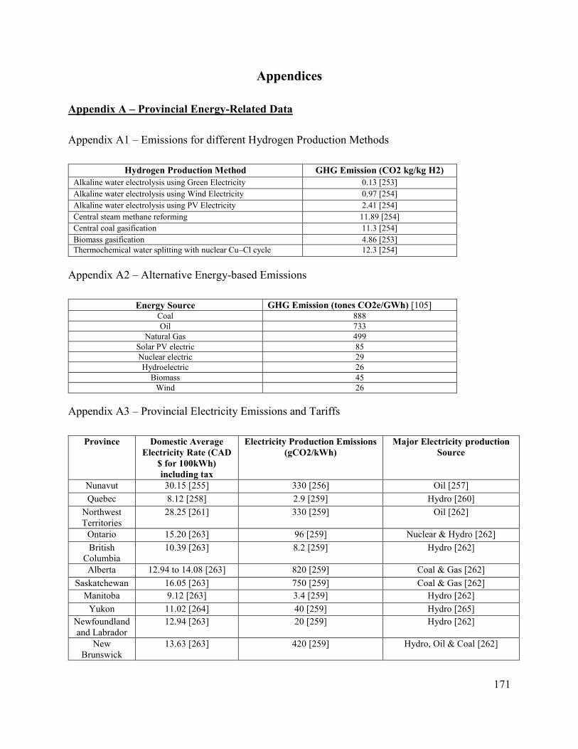
171

Appendices

Appendix A – Provincial Energy-Related Data

Appendix A1 – Emissions for different Hydrogen Production Methods

Hydrogen Production Method GHG Emission (CO2 kg/kg H2)

Alkaline water electrolysis using Green Electricity 0.13 [253]

Alkaline water electrolysis using Wind Electricity 0.97 [254]

Alkaline water electrolysis using PV Electricity 2.41 [254]

Central steam methane reforming 11.89 [254]

Central coal gasification 11.3 [254]

Biomass gasification 4.86 [253]

Thermochemical water splitting with nuclear Cu–Cl cycle 12.3 [254]

Appendix A2 – Alternative Energy-based Emissions

Energy Source GHG Emission (tones CO2e/GWh) [105] Coal 888

Oil 733

Natural Gas 499

Solar PV electric 85

Nuclear electric 29

Hydroelectric 26

Biomass 45

Wind 26

Appendix A3 – Provincial Electricity Emissions and Tariffs

Province Domestic Average

Electricity Rate (CAD

$ for 100kWh)

including tax

Electricity Production Emissions

(gCO2/kWh)

Major Electricity production

Source

Nunavut 30.15 [255] 330 [256] Oil [257]

Quebec 8.12 [258] 2.9 [259] Hydro [260]

Northwest

Territories

28.25 [261] 330 [259] Oil [262]

Ontario 15.20 [263] 96 [259] Nuclear & Hydro [262]

British

Columbia

10.39 [263] 8.2 [259] Hydro [262]

Alberta 12.94 to 14.08 [263] 820 [259] Coal & Gas [262]

Saskatchewan 16.05 [263] 750 [259] Coal & Gas [262]

Manitoba 9.12 [263] 3.4 [259] Hydro [262]

Yukon 11.02 [264] 40 [259] Hydro [265]

Newfoundland

and Labrador

12.94 [263] 20 [259] Hydro [262]

New

Brunswick

13.63 [263] 420 [259] Hydro, Oil & Coal [262]

172

Nova Scotia 16.83 [263] 700 [259] Coal [262]

Prince Edward

Island

17.34 [263] 22 [259] Wind [262]

Appendix A4 – Other Utility Tariffs for Households

Natural Gas price Gasoline

Province Base ($/month) level 1 level2 level3 ($/100 liter)

Quebec (Montreal) 16.57 $0.2674/ m3

(~900m3)

$0.1829 /m3

(900m3~2170 m3)

$0.15995/m3

(2179 m3~)

107.00

Ontario (Ottawa) 20.00 $ 0.2504/m3 106.10

British Columbia (Mainland) 12.06 $ 7.16 / Gj 121.60

Alberta (Edmonton) 30.16 $ 1.83/GJ 105.60

Saskatchewan (Saskatoon) 23.20 $ 0.2311/m3 107.80

Manitoba (Winnipeg) 14.00 $ 0.2235/m3 112.70

Nova Scotia (Halifax) 21.87 $ 18.075/GJ 103.10

Source: On-line databases of provincial utility providers (Accessed in November 2017)

Appendix B – Characteristics of Representing Vehicles

Appendix B1 – Maintenance and Repair Cost Data for Vehicles Considered in the Study

Based on cars.com Cars.com, 2016, the maintenance cost as at 2016 from year 1 to 5 years are as below,

Year 00

(CAD$)6

Year 01

(CAD$)7

Year 02

(CAD$)8

Year 03

(CAD$)9

Year 04

(CAD$)10

Year 05

(CAD$)11

Yaris 4DR LE 2016 (1500 cc) 108 247 2,061 975 880 4,272

Hyundai Tucson FCEV 4 DR5 0 0 0 0 802 4,789

Nissan Leaf S 5DR 213 357 2,412 1,008 802 4,789

5 Hyundai maintenance cost is assumed as similar to the Nissan leaf due to the similar power train options. But the

capital cost covered the cost of maintenance and cost of fuel for the next 03 years, and the last 02 years are assumed

to be similar to the Nissan Leaf. 6,7,8,9,10,11Source: [266]

Appendix B2 – Vehicle Specifications

Nissan Leaf S 5DR1 Hyundai Tucson FCEV2 Toyota Yaris 4DR LE3 Unit

Year of Manufacturing 2016 2016 2016

Range 133 500 500 Km/ per re-fueling cycle

Consumption 34 kWh/100km 77 km/kg 12.32 km/l

Size of Battery Pack 30 - - kWh

Cost of Vehicle 26,688 66,9404 21,151 CAD $

Engine power torque 107 134 106 hp

Gross Weight 1481 1882 1515 kg 1 Source [203] 2 Source [204] 3 Source [205] 4 This includes the fuel cost and general maintenance cost for the first 03 years of the vehicle.

173

Appendix C – Intermediate Results of the Life Cycle Assessment

Appendix C1: The life cycle impacts of the vehicle except for the operational phase

Electric vehicle ICEV HFCV -

Weight kg 1293 201 NA 1392 NA NA 1578 NA NA

Name Units Con. RM EoL T_LCIA_EV Con. RM EoL T_LCIA_ICEV Con. RM EoL T_LCIA_HFCV

Inputs

Total Energy GJ 26.1 16.9 15.0 58.1 41.3 4.2 10.5 56.0 87.3 2.6 10.5 100.4

Water m^3 26.3 10.4 3.1 39.8 18.3 0.3 2.2 20.8 28.9 0.8 2.2 31.9

Non fossil fuels GJ 5.3 2.1 1.7 9.1 3.6 0.0 1.2 4.8 7.5 0.2 1.2 8.8

Renewable GJ 3.4 1.6 0.8 5.7 2.2 0.0 0.5 2.7 4.5 0.1 0.5 5.1

Biomass GJ 0.1 0.1 0.0 0.2 0.1 0.0 0.0 0.1 0.2 0.0 0.0 0.2

Fossil Fuels GJ 50.4 15.0 13.3 78.7 37.7 4.1 9.3 51.2 79.5 2.4 9.3 91.3

Petroleum

Fuels GJ 6.3 2.0 0.2 8.5 4.2 2.8 0.1 7.2 9.2 0.5 0.1 9.7

Natural Gas

Fuels GJ 23.3 8.8 9.0 41.1 15.7 1.1 6.3 23.1 44.6 1.4 6.3 52.3

Coal Fuels GJ 23.3 4.0 4.1 31.4 17.8 0.2 2.9 20.9 25.2 0.6 2.9 28.7

Nuclear GJ 1.9 0.5 0.9 3.4 1.4 0.0 0.7 2.1 3.0 0.1 0.7 3.7

Outputs

CO2 kg 3589.0 968.0 902.1 5459.1 2654.9 221.0 640.0 3515.9 5371.8 127.8 640.0 6139.5

VOC kg 3.2 13.8 1.7 18.6 2.5 9.7 1.2 13.4 2.9 9.6 1.2 13.7

CO kg 17.9 68.9 0.5 87.3 13.8 0.1 0.3 14.3 15.7 0.2 0.3 16.2

NOx kg 4.2 1.4 0.8 6.5 3.0 0.4 0.6 4.0 6.0 0.2 0.6 6.8

PM10 kg 1.8 0.7 0.1 2.7 1.4 0.1 0.1 1.6 2.0 0.1 0.1 2.2

PM2.5 kg 0.8 0.2 0.1 1.2 0.7 0.0 0.1 0.8 0.9 0.0 0.1 1.0

SOx kg 24.0 12.6 1.1 37.6 13.9 1.4 0.8 16.1 20.8 3.7 0.8 25.2

CH4 kg 9.1 2.4 2.2 13.7 6.6 0.5 1.6 8.7 13.8 0.5 1.6 15.9

N2O g 79.9 21.1 20.0 121.0 55.8 5.3 14.1 75.2 127.4 4.0 14.1 145.5

BC g 29.2 16.5 5.9 51.7 19.1 2.9 4.2 26.2 42.9 3.1 4.2 50.2

POC g 46.5 20.1 13.8 80.4 33.3 3.2 9.8 46.2 79.9 2.4 9.8 92.0

H2 9 0 0 0 0 0 0 0 0 0 0 0 0

Con. – Construction phase

RM – Regular maintenance

EoL – End of life T_LCIA_V – Total life cycle impacts of the vehicle (Except the operation phase)

174

Appendix C2: Vehicle Operational Impacts for the Considered Life Cycle of the Vehicle

Appendix C3 Total life cycle inventory of the different fuel options

Input

Inventory

Province-wise energy and resources consumption for EVs (Complete Life Cycle Inventory) Raw materials and Energy for HFCVs ICEVs

Unit BC MN QC NF YK NWT ON NB SK NS AB PEI NU Natural

Gas Nuclear Coal Biomass Electrolysis

Water m^3 5.E+02 5.E+04 5.E+02 5.E+02 5.E+02 3.E+02 2.E+02 2.E+02 1.E+02 1.E+02 4.E+01 4.E+01 3.E+02 9.E+01 2.E+02 9.E+01 6.E+01 4.E+01 5.E+02

Non fossil

fuels GJ 1.E+05 1.E+05 1.E+05 1.E+05 1.E+05 5.E+04 1.E+05 9.E+04 2.E+04 5.E+04 2.E+04 1.E+05 6.E+03 2.E+04 2.E+05 4.E+02 5.E+05 2.E+05 3.E+05

Renewable GJ 1.E+05 1.E+05 1.E+05 1.E+05 1.E+05 5.E+04 4.E+04 5.E+04 2.E+04 5.E+04 2.E+04 1.E+05 3.E+03 1.E+04 4.E+02 2.E+02 5.E+05 2.E+05 3.E+05

Biomass GJ 3.E+04 2.E-01 5.E+03 3.E-01 2.E+00 2.E+04 5.E+03 2.E+04 2.E+00 2.E+04 1.E+04 5.E+03 1.E+02 4.E+02 2.E+01 6.E+00 5.E+05 3.E-01 3.E+05

Fossil Fuels GJ 7.E+03 8.E+01 2.E+02 2.E+04 3.E+04 2.E+05 1.E+04 1.E+05 2.E+05 2.E+05 3.E+05 4.E+03 1.E+06 3.E+05 6.E+03 5.E+02 3.E+04 8.E+02 3.E+05

Unit BC MN QC NF YK NWT ON NB SK NS AB PEI NU

Natural

Gas Nuclear Coal Biomass Electrolysis

Water m^3 468 54419 485 485 474 231 165 132 102 83 4 1 215 57 130 63 29 7 496

Non fossil fuels GJ 131311 110160 114016 104719 101449 46074 108857 88615 19938 48370 18940 112914 5913 24294 198187 352 462436 247734 346827

Renewable GJ 131311 110160 114016 104682 101392 45573 43686 48750 19878 48198 18854 112914 2649 10966 435 159 462436 247734 346827

Biomass GJ 29908 0 4985 0 2 16065 4990 19946 2 24929 9973 4985 105 427 17 6 462436 0 346827

Fossil Fuels GJ 6787 0 126 16966 26643 209965 13852 104581 231887 228582 254690 3770 1321920 313796 6191 446 32750 755 280765

Petroleum Fuels GJ 4004 0 110 13345 20023 183416 322665 28058 2361 42895 12568 3445 1211760 2765 1177 6860 11547 663 109845

Natural Gas Fuels GJ 2731 0 1 3463 6383 24443 12752 26671 88528 38044 104042 285 977670 247734 2687 1417 16198 83 139524

Coal Fuels GJ 51 0 1 157 237 2130 777 49853 141005 147614 138030 40 14 59 2 429 5 0 23469

Nuclear GJ 12 0 0 37 56 502 65171 39865 0 172 87 9 3 13 198 193 1 0 2768Impacts of

ICEV

Total CO2 kg 56 0 6 1 2010 16524 812 2295 18727 6021 19829 296 104652 19984 459 38812 2312 55 30559

VOC kg 0.0 0.0 0.0 0.1 0.2 1.3 0.2 0.1 1.8 0.1 2.1 0.1 8.1 0 0 3 2 0 26

CO kg 0.1 0.0 1.5 0.4 0.6 4.5 2.2 0.4 6.1 0.7 10.0 1.5 26.4 0 1 2 5 0 166

NOX kg 0.1 0.0 0.3 5.3 8.1 72.7 1.2 1.1 13.2 2.7 18.7 1.6 469.3 0 1 9 8 0 36

PM10 kg 0.1 0.0 0.6 0.2 0.3 3.1 0.7 0.2 2.2 0.4 3.6 0.7 19.8 1 0 4 1 0 5

PM2.5 kg 0.0 0.0 0.2 0.2 0.3 2.2 0.2 0.1 0.9 0.3 1.4 0.2 14.3 1 0 1 1 0 2

SOX kg 0.0 0.0 0.2 3.6 5.6 50.7 0.5 4.6 34.1 13.2 36.4 1.1 331.6 17 1 5 29 0 25

CH4 kg 0.0 0.0 0.2 1.7 2.8 19.8 2.5 0.2 26.4 0.2 28.6 0.5 116.8 60 1 60 5 0 39

N2O g 2047 0 20 12 19 143 32 33 347 88 412 684 887 413 7 236 1652 1 10993

BC g 2329 0 26 13 20 173 33 8 62 17 128 30 1112 64 8 42 11231 1 81

POC g 5478 0 61 15 23 187 73 18 158 35 299 64 1177 124 14 118 229 6 492

H2 g 0 0 0 0 0 0 0 0 0 0 0 0 0 2147 11231 11231 168 9249 0

Input for

ICEV

operation

Impacts of HFCV vehicle operation

Province-wise raw material group and environmental impacts based on grid electricity mix (Total operational impacts)

Province-wise raw material group and environmental impacts based on grid electricity mix (Total operational impacts)

Raw materials for HFCV vehicle operation

175

Petroleum

Fuels GJ 4.E+03 8.E+00 1.E+02 1.E+04 2.E+04 2.E+05 3.E+05 3.E+04 2.E+03 4.E+04 1.E+04 3.E+03 1.E+06 3.E+03 1.E+03 7.E+03 1.E+04 7.E+02 1.E+05

Natural Gas

Fuels GJ 3.E+03 4.E+01 4.E+01 4.E+03 6.E+03 2.E+04 1.E+04 3.E+04 9.E+04 4.E+04 1.E+05 3.E+02 1.E+06 2.E+05 3.E+03 1.E+03 2.E+04 1.E+02 1.E+05

Coal Fuels GJ 8.E+01 3.E+01 3.E+01 2.E+02 3.E+02 2.E+03 8.E+02 5.E+04 1.E+05 1.E+05 1.E+05 7.E+01 5.E+01 9.E+01 3.E+01 5.E+02 3.E+01 3.E+01 2.E+04

Nuclear GJ 2.E+01 3.E+00 4.E+00 4.E+01 6.E+01 5.E+02 7.E+04 4.E+04 3.E+00 2.E+02 9.E+01 1.E+01 7.E+00 2.E+01 2.E+02 2.E+02 5.E+00 4.E+00 3.E+03

Output

Inventory Province-wise environmental impacts of EVs (Complete Life Cycle Inventory) Method-wise impacts of HFCVs ICEVs

Total CO2 kg 6.E+03 5.E+03 5.E+03 5.E+03 7.E+03 2.E+04 6.E+03 8.E+03 2.E+04 1.E+04 3.E+04 6.E+03 1.E+05 3.E+04 7.E+03 4.E+04 8.E+03 6.E+03 3.E+04

VOC kg 2.E+01 2.E+01 2.E+01 2.E+01 2.E+01 2.E+01 2.E+01 2.E+01 2.E+01 2.E+01 2.E+01 2.E+01 3.E+01 1.E+01 1.E+01 2.E+01 2.E+01 1.E+01 4.E+01

CO kg 9.E+01 9.E+01 9.E+01 9.E+01 9.E+01 9.E+01 9.E+01 9.E+01 9.E+01 9.E+01 1.E+02 9.E+01 1.E+02 2.E+01 2.E+01 2.E+01 2.E+01 2.E+01 2.E+02

NOX kg 7.E+00 6.E+00 7.E+00 1.E+01 1.E+01 8.E+01 8.E+00 8.E+00 2.E+01 9.E+00 3.E+01 8.E+00 5.E+02 7.E+00 8.E+00 2.E+01 1.E+01 7.E+00 4.E+01

PM10 kg 3.E+00 3.E+00 3.E+00 3.E+00 3.E+00 6.E+00 3.E+00 3.E+00 5.E+00 3.E+00 6.E+00 3.E+00 2.E+01 3.E+00 2.E+00 6.E+00 3.E+00 2.E+00 7.E+00

PM2.5 kg 1.E+00 1.E+00 1.E+00 1.E+00 1.E+00 3.E+00 1.E+00 1.E+00 2.E+00 1.E+00 3.E+00 1.E+00 2.E+01 2.E+00 1.E+00 2.E+00 2.E+00 1.E+00 3.E+00

SOX kg 4.E+01 4.E+01 4.E+01 4.E+01 4.E+01 9.E+01 4.E+01 4.E+01 7.E+01 5.E+01 7.E+01 4.E+01 4.E+02 4.E+01 3.E+01 3.E+01 5.E+01 3.E+01 4.E+01

CH4 kg 1.E+01 1.E+01 1.E+01 2.E+01 2.E+01 3.E+01 2.E+01 1.E+01 4.E+01 1.E+01 4.E+01 1.E+01 1.E+02 8.E+01 2.E+01 8.E+01 2.E+01 2.E+01 5.E+01

N2O g 2.E+03 1.E+02 1.E+02 1.E+02 1.E+02 3.E+02 2.E+02 2.E+02 5.E+02 2.E+02 5.E+02 8.E+02 1.E+03 6.E+02 2.E+02 4.E+02 2.E+03 1.E+02 1.E+04

BC g 2.E+03 5.E+01 8.E+01 6.E+01 7.E+01 2.E+02 8.E+01 6.E+01 1.E+02 7.E+01 2.E+02 8.E+01 1.E+03 1.E+02 6.E+01 9.E+01 1.E+04 5.E+01 5.E+01

POC g 6.E+03 8.E+01 1.E+02 1.E+02 1.E+02 3.E+02 2.E+02 1.E+02 2.E+02 1.E+02 4.E+02 1.E+02 1.E+03 2.E+02 1.E+02 2.E+02 3.E+02 1.E+02 5.E+02

H2 g 0.E+00 0.E+00 0.E+00 0.E+00 0.E+00 0.E+00 0.E+00 0.E+00 0.E+00 0.E+00 0.E+00 0.E+00 0.E+00 2.E+03 1.E+04 1.E+04 2.E+02 9.E+03 0.E+00

Appendix C4: Life Cycle Cost Assessment of Electric Vehicles

Province

Average Electricity

Domestic rate (CAD $ for

100kWh) including tax

Infrastructure cost

(Annualized) (CAD

$ for 100kWh)

Total electricity retail

price with 12% margin

(CAD$ for 100kWh)

Electricity cost for 5yr

operation (CAD $)

LCC for EV for 5 year

life span (CAD $)

Nunavut 30.15 2.92 37.03 11332.07 36835.74

Quebec 8.12 2.92 12.36 3781.95 29285.62

Northwest Territories 28.25 2.92 34.90 10680.90 36184.58

Ontario 15.2 2.92 20.29 6208.40 31712.08

British Columbia 10.39 2.92 14.90 4559.92 30063.60

Alberta 13.51 2.92 18.40 5629.21 31132.88

Saskatchewan 16.05 2.92 21.24 6499.72 32003.39

Manitoba 9.12 2.92 13.48 4124.67 29628.34

Yukon 11.02 2.92 15.61 4775.83 30279.51

Newfoundland and Labrador 12.94 2.92 17.76 5433.86 30937.53

New Brunswick 13.63 2.92 18.53 5670.33 31174.01

Nova Scotia 16.83 2.92 22.11 6767.04 32270.71

Prince Edward Island 17.34 2.92 22.69 6941.83 32445.50

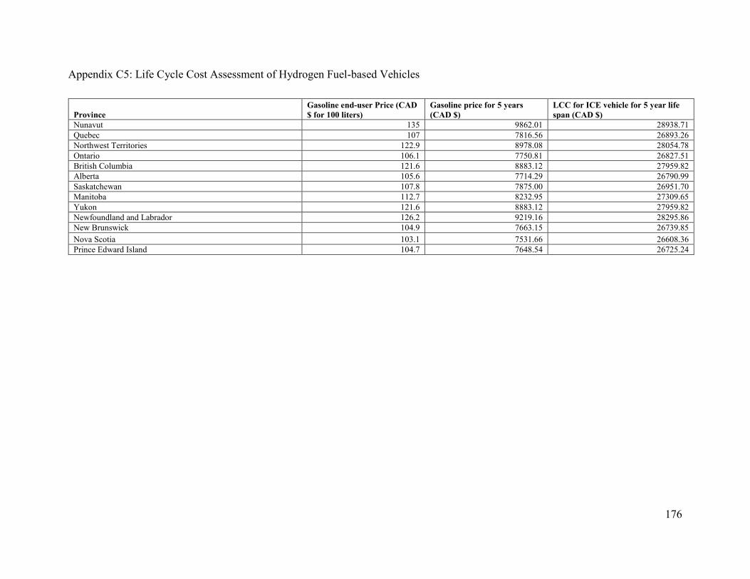
176

Appendix C5: Life Cycle Cost Assessment of Hydrogen Fuel-based Vehicles

Province

Gasoline end-user Price (CAD

$ for 100 liters)

Gasoline price for 5 years

(CAD $)

LCC for ICE vehicle for 5 year life

span (CAD $)

Nunavut 135 9862.01 28938.71

Quebec 107 7816.56 26893.26

Northwest Territories 122.9 8978.08 28054.78

Ontario 106.1 7750.81 26827.51

British Columbia 121.6 8883.12 27959.82

Alberta 105.6 7714.29 26790.99

Saskatchewan 107.8 7875.00 26951.70

Manitoba 112.7 8232.95 27309.65

Yukon 121.6 8883.12 27959.82

Newfoundland and Labrador 126.2 9219.16 28295.86

New Brunswick 104.9 7663.15 26739.85

Nova Scotia 103.1 7531.66 26608.36

Prince Edward Island 104.7 7648.54 26725.24

177

Appendix D – EV-RI Location Allocation Data

Appendix D1 – Site Inspection Form for Site-specific Data Gathering

178

Appendix D2 – Multi-objective Problem Solving using IBM ILOG CPLEX Source Code

/********************************************* * OPL 12.8.0.0 Model * Author: piyaru1 * Creation Date: Feb 11, 2019 at 12:46:51 PM *********************************************/ // parameters int n = ...; //No of demand points int m = ...; //No of re-charging stations range route = 1..n; range EVRI = 1..m; float distance[route,EVRI]=...; float demand_cap[route]=...; float supply_cap[EVRI]=...; float Cap_cost[EVRI]=...; float Var_cost[EVRI]=...; //variables dvar float+ x[route][EVRI]; // Decision variable minimize ((sum (j in EVRI, i in route)x[i][j]*Var_cost[j]/10)+ sum (i in route, j in EVRI) distance[i][j]*x[i][j]); // fitness function subject to { forall(i in route) available_demand_cap: sum(j in EVRI) x[i][j] == demand_cap[i]; // Demand constraint forall(j in EVRI) available_supply_cap: sum(i in route) x[i][j] <= supply_cap[j]; // Supply constraint }

/********************************************* * OPL 12.8.0.0 Data * Author: piyaru1 * Creation Date: Feb 11, 2019 at 12:46:51 PM *********************************************/ n=32975; // Number of routes m=14; // Number of potential EV-RI facilities SheetConnection my_sheet ("Worksheet2.xlsx"); SheetConnection my_sheet1 ("DEF.xlsx"); distance from SheetRead(my_sheet,"'Sheet1'!B2:O32976"); // Output from the ArcGIS model demand_cap from SheetRead(my_sheet,"'Sheet1'!P2:P32976"); // Array changes with the time period supply_cap from SheetRead(my_sheet,"'Sheet1'!S2:S15"); // Location-based capacity inputs Cap_cost from SheetRead(my_sheet,"'Sheet1'!T2:T15"); // Location-based cost inputs Var_cost from SheetRead(my_sheet,"'Sheet1'!U2:U15"); // Location-based cost inputs

x to SheetWrite(my_sheet1,"'Sheet1'!B2:O32976");

179

Appendix D3 – Model inputs for the case study

Paving and land preparation cost (CAD/sq.meter) Cp $135.00

land required per each EV-RI - Fast charging (sq.m/unit) LI 60

EV-RI unit costs

Paving cost per each EV-RI (CAD/fast charging unit) CI $8,100.00

Unit cost of Electric vehicle infrastructure - Fast Charging

(CAD/unit)

ρ1 $40,000

Installation and Labour cost (CAD/unit)

$50,000

Total DC-FC related costs

$98,100

Annual networking fee (CAD/unit.year)

$225

Annual maintenance (CAS/unit.year)

$200

Total operating cost per year per unit (CAD/unit.year) (Except the

cost of electricity)

$425

Current electricity cost ($/kWh) ꙋ0 0.15

kW power consumption of the vehicle I (kWh/100 km) λi 34

Useful power supply from EV-RI- Fast Charging(kW/unit) Pu1 50

Average recharging sessions per year per unit

3600

Vehicle types (TIPSLab-UBC)

Battery operated vehicles (Electricity only) 160 km

maximum fast charging 80%

Battery capacity 30 kWh

Consumption 340 Wh/km

Therefore, Recharge capacity per time 15.2 kWh/recharge

Land mortgage term 20 years

Inflation/ discount rate 3.50%

180

Appendix D4 : Total investment cost and payback calculation based on the optimization results

Location

ID

Neighbourhood Multi-period EV-RI

capacities in terms of DC-FC

units (NUmt ) and potential

locations (Optimization

Results)

Multi-period EV-RI

capacities improvement in

terms of DC-FC units

Lan

gitu

de

Lati

tud

e

TAZ

No

.

Lan

d c

ost

Fac

tor

(LC

m)

(CA

D/s

q.m

)

Max

. Cap

acit

y (N

Um

)

Max

imu

m v

ehic

le c

apac

ity

New DC-FC investment Land acquisition costs

2020

2030

2040

2050

2020

2030

2040

2050

(20

20)

(20

30)

(20

40)

(20

50)

(20

20)

(20

30)

(20

40)

(20

50)

1 PANDOSY 1 6 10 10 1 5 4 0 -119.491 49.86083 107 2500 10 36000 $98,100 $490,500 $392,400 $0 $9,174 $55,041 $82,562 $27,521

2 UNIVERSITY PLAZZA 0 1 5 10 0 1 4 5 -119.389 49.92223 154 2900 10 36000 $0 $98,100 $392,400 $490,500 $0 $10,641 $53,206 $95,771

3 MCCURDY CORNER 0 0 1 9 0 0 1 8 -119.405 49.90209 63 3200 20 72000 $0 $0 $98,100 $784,800 $0 $0 $11,742 $105,679

4 COOPER CENTRE 0 0 0 2 0 0 0 2 -119.445 49.88261 52 3500 10 36000 $0 $0 $0 $196,200 $0 $0 $0 $25,686

5 BANKS-SPRINGFIELD 0 0 0 1 0 0 0 1 -119.425 49.88871 55 3500 10 36000 $0 $0 $0 $98,100 $0 $0 $0 $12,843

6 CAPRI CENTRE MALL 0 0 5 16 0 0 5 11 -119.475 49.88117 34 3200 16 57600 $0 $0 $490,500 $1,079,100 $0 $0 $58,710 $187,873

7 ORCHARD PLAZA 0 0 0 0 0 0 0 0 -119.469 49.88195 35 3600 10 36000 $0 $0 $0 $0 $0 $0 $0 $0

8 SPALL PLAZA 0 0 0 7 0 0 0 7 -119.458 49.8821 28 3300 16 57600 $0 $0 $0 $686,700 $0 $0 $0 $84,763

9 GLENMORE 1 3 14 20 1 2 11 6 -119.443 49.91531 160 2500 20 72000 $98,100 $196,200 $1,079,100 $588,600 $9,174 $27,521 $119,256 $146,776

10 RICHTER 0 0 0 4 0 0 0 4 -119.49 49.88477 24 3800 10 36000 $0 $0 $0 $392,400 $0 $0 $0 $55,775

11 CLEMENT 0 3 10 10 0 3 7 0 -119.476 49.89292 15 2600 10 36000 $0 $294,300 $686,700 $0 $0 $28,621 $95,404 $66,783

12 SPRINGFIELD 1 4 20 20 1 3 16 0 -119.456 49.87627 50 2600 20 72000 $98,100 $294,300 $1,569,600 $0 $9,540 $38,162 $181,269 $143,107

13 BANKS 0 0 0 1 0 0 0 1 -119.428 49.8836 58 3600 10 36000 $0 $0 $0 $98,100 $0 $0 $0 $13,210

14 RUTLAND 1 9 20 20 1 8 11 0 -119.398 49.89007 77 2000 20 72000 $98,100 $784,800 $1,079,100 $0 $7,339 $66,049 $139,437 $73,388

Network Investment Cost (CAD) $392,400 $2,158,200 $5,787,900 $4,414,500 $35,226 $226,035 $741,586 $1,039,175

181

Appendix E – Household Related Data

Appendix E1 – Residential Building As-Is Drawing

(Source: AuthenTech Homes Ltd.)

Appendix E2 – Specifications of Base-Case Residential Building

Building parameters (Reference case)

Year of manufacturing 2017

Total floor area 2,690 ft2

Orientation Northwest

Thermal zone settings Single Thermostat

Main floor set points: Daytime – 69.80F & night time – 64.40F

Cooling set point: 770F

Night time set back duration: 8 hrs

Occupancy 2 – Adults & 1 – Child (50% occupancy time)

Foundation 8” reinforced concrete, R-22 insulation

Basement slab 4” concrete

Exterior wall (Section 1) 2”×6” wood studs @ 24” OC, 3/8” OSB sheeting, R-20 insulation, ½” drywall

Interior wall 2”×4” wood studs, ½” drywall

Ground floor Engineered I joist 11 7/8” @ 19.2” OC, ¾” plywood, R-11 insulation

Ceiling R-22 Batt, R-40 blown in insulation, ½” drywall

Roof Engineered trusses (wood), 1/2” OSB sheeting, Asphalt

Windows Vinyl double glazed windows c/w 180 low-E Air Tightness: 0.2 L/s.m2

Space heating system Energy star rated dual fuel (Natural Gas & Electric) EF - 92.1%, 56000 BTU/hr,

switching temperature 350F & Natural gas fireplace 2kW, 6824.28 BTU/hr 30% SS

Space cooling system Energy star rated central split system, (electric), 14SEER

182

Washer & Dryer Standard (916kWh/year)

Heat recovery system Single stage PSC blower

Refrigerator Standard (639kWh/year)

Stove & Oven Standard Energy Star rated cooker and oven (565kWh/year)

Hot water system Energy star rated natural gas hot water tank 1EF (Hot water temperature: 1310F)

(60Gal)

Other electricity use 12kWh/day

Lighting 25%-75% LED or CFL

Solar(PV) electricity

generator

Not available

House construction cost

(CAD)7

414,032.99

Appendix E3 Results of EV Incentive Scheme Ranking

7 Purchase cost excluding the land value and the profit of the builders, contractors and developers.

183

Appendix E4 - Building Retrofit Options

Quebec**** Ontario*** British Columbia* Alberta** Saskatchewan Manitoba Nova Scotia## B

uild

ing

retr

ofi

t in

cen

tive

scem

es

An

nu

aliz

ed c

on

sum

er c

ost

savi

ngs

An

nu

aliz

ed G

HG

red

uct

ion

:

H2

D (

kgC

O2

e/ye

ar)

An

nu

aliz

ed c

on

sum

er c

ost

savi

ngs

An

nu

aliz

ed G

HG

red

uct

ion

: H

2D

(kg

CO

2e/

year

)

An

nu

aliz

ed c

on

sum

er c

ost

sa

vin

gs

An

nu

aliz

ed G

HG

red

uct

ion

: H

2D

(kg

CO

2e/

year

)

An

nu

aliz

ed c

on

sum

er c

ost

sa

vin

gs

An

nu

aliz

ed G

HG

red

uct

ion

:

H2

D (

kgC

O2

e/ye

ar)

An

nu

aliz

ed c

on

sum

er c

ost

savi

ngs

An

nu

aliz

ed G

HG

red

uct

ion

: H

2D

(kg

CO

2e/

year

)

An

nu

aliz

ed c

on

sum

er c

ost

savi

ngs

An

nu

aliz

ed G

HG

red

uct

ion

: H

2D

(kg

CO

2e/

year

)

An

nu

aliz

ed c

on

sum

er c

ost

sa

vin

gs

An

nu

aliz

ed G

HG

red

uct

ion

: H

2D

(kg

CO

2e/

year

)

Null 0.00 0.00 0.00 0.00 0.00 0.00 0.00 0.00 0.00 0.00 0.00 0.00 0.00 0.00

R1 973.33 4.61 698.08 35.63 933.74 6.42 838.38 409.70 950.49 275.17 982.83 7.03 593.33 397.80

R2 188.69 13.34 98.77 -127.20 150.43 3.71 170.96 -1414.50 286.63 -1249.05 134.31 15.13 125.23 -1053.52

R3 36.17 0.43 25.96 31.33 40.59 1.65 52.80 219.53 22.95 224.26 48.57 0.50 32.26 167.19

R4 -727.55 96.69 -72.54 -299.04 99.34 46.95 -956.63 -4562.11 -416.33 -4579.52 -883.03 132.07 -

172.85 -2767.49

R5 352.22 8.13 232.88 256.17 341.79 18.45 319.16 2255.10 160.50 2219.65 120.10 10.16 191.59 1739.49

R1+R2 1162.02 17.95 796.86 -91.57 1084.17 10.13 1009.35 -1004.81 1237.12 -973.89 1117.14 22.16 718.56 -655.72

R1+R3 1009.51 5.04 724.05 66.95 974.34 8.07 891.19 629.23 973.45 499.42 1031.41 7.54 625.60 564.98

R1+R4 245.79 101.29 625.55 -263.42 1033.08 53.37 -118.24 -4152.41 534.16 -4304.36 99.80 139.11 420.48 -2369.69

R1+R5 1325.55 12.74 930.96 291.80 1275.53 24.87 1157.54 2664.80 1110.99 2494.82 1102.93 17.19 784.92 2137.29

R2+R3 224.86 13.77 124.74 -95.87 191.02 5.36 223.77 -1194.97 309.58 -1024.80 182.88 15.63 157.49 -886.33

R2+R4 -538.86 110.02 26.24 -426.24 249.77 50.66 -785.66 -5976.62 -129.70 -5828.58 -748.72 147.20 -47.62 -3821.01

R2+R5 540.90 21.47 331.65 128.98 492.22 22.16 490.12 840.60 447.12 970.60 254.40 25.29 316.81 685.97

R3+R4 -691.37 97.12 -46.57 -267.71 139.94 48.60 -903.82 -4342.58 -393.37 -4355.27 -834.45 132.58 -

140.58 -2600.31

184

R3+R5 388.39 8.57 258.84 287.50 382.38 20.10 371.96 2474.64 183.45 2443.91 168.67 10.66 223.85 1906.67

R4+R5 -375.33 104.82 160.34 -42.87 441.13 65.40 -637.47 -2307.01 -255.83 -2359.87 -762.93 142.23 18.74 -1028.00

R1+R2+R3 1198.20 18.38 822.82 -60.25 1124.77 11.78 1062.15 -785.27 1260.08 -749.63 1165.71 22.67 750.83 -488.53

R1+R2+R4 434.47 114.63 724.32 -390.61 1183.51 57.08 52.72 -5566.92 820.79 -5553.41 234.11 154.24 545.71 -3423.21

R1+R2+R5 1514.24 26.08 1029.73 164.60 1425.96 28.58 1328.51 1250.30 1397.62 1245.76 1237.24 32.32 910.15 1083.77

R1+R3+R4 281.96 101.73 651.51 -232.09 1073.68 55.02 -65.44 -3932.88 557.12 -4080.10 148.38 139.61 452.75 -2202.51

R1+R3+R5 1361.72 13.17 956.92 323.13 1316.12 26.52 1210.35 2884.33 1133.94 2719.07 1151.50 17.69 817.18 2304.47

R1+R4+R5 598.00 109.43 858.42 -7.24 1374.87 71.82 200.92 -1897.31 694.66 -2084.71 219.90 149.27 612.07 -630.20

R2+R3+R4 -502.68 110.46 52.20 -394.91 290.37 52.31 -732.86 -5757.09 -106.75 -5604.32 -700.15 147.71 -15.36 -3653.82

R2+R3+R5 577.08 21.90 357.61 160.30 532.81 23.81 542.93 1060.13 470.08 1194.85 302.98 25.79 349.08 853.16

R2+R4+R5 -186.64 118.15 259.11 -170.07 591.56 69.11 -466.50 -3721.51 30.80 -3608.93 -628.63 157.36 143.97 -2081.52

R3+R4+R5 -339.16 105.25 186.30 -11.54 481.72 67.05 -584.66 -2087.48 -232.88 -2135.62 -714.36 142.74 51.00 -860.82

R1+R2+R3+R4 470.65 115.06 750.28 -359.29 1224.11 58.73 105.52 -5347.39 843.75 -5329.16 282.69 154.74 577.98 -3256.02

R1+R2+R3+R5 1550.41 26.51 1055.70 195.93 1466.55 30.23 1381.31 1469.83 1420.57 1470.02 1285.81 32.82 942.41 1250.95

R1+R2+R4+R5 786.69 122.76 957.20 -134.44 1525.30 75.53 371.88 -3311.81 981.29 -3333.76 354.21 164.40 737.30 -1683.72

R1+R3+R4+R5 634.18 109.86 884.39 24.08 1415.46 73.47 253.72 -1677.78 717.61 -1860.45 268.47 149.77 644.33 -463.02

R2+R3+R4+R5 -150.47 118.59 285.08 -138.74 632.15 70.76 -413.70 -3501.98 53.75 -3384.67 -580.05 157.86 176.23 -1914.34

R1+R2+R3+R4+R5 (H2M) 822.86 123.20 983.16 -103.11 1565.89 77.18 424.68 -3092.28 1004.24 -3109.50 402.78 164.90 769.56 -1516.54

185

Appendix F –PDM Selection Process

Appendix F1 – Data Collection Form to Collect the Stakeholder Perception of Different Attributes

Section Attributes Description Very

Important

Better to

have it

Not that

important

Not

Applicable

Project

characteristics

Scope definition Having an exact goal about the EV-RI development

Project schedule Having an exact schedule for the development

Contract Strategy Having an exact payment method for the EV-RI development

Complexity The complexity of the development process and evaluate the

technical know-how of the development

Owners pre-

requests

Constructability

studies

Do a feasibility study beforehand

Value engineering

studies

Do value engineering to optimize the construction procedure

Contract packaging Do the modular type of construction by having multiple

subcontractors to distribute work

Contract awarding

criteria

Evaluate contract awarding criteria before starting the procurement

process

Cost Sharing Share the cost of the recharging infrastructure with a third party

(having a separate funding partner)

Owners

preferences

Responsibility Share the responsibility of the recharging infrastructure with a

third party (having a construction manager for the project)

Design control Control the design by the owner or having it contracted to a third

party

Involvement after

awarding

Involve with decisions during the construction phase of the project

Risk

Change orders Change the initial design during the construction

Risk-sharing Share the risk of the recharging infrastructure with a third party

(having separate insurance to cover the risk)

Quality Quality control and

quality assurance

Check the quality of the final product

186

Appendix F2 – Judgment Matrix for LoE

Attribute No. The initial deployment stage The way forward to the business-as-

usual stage

Stakeholder

Category 1

Stakeholder

Category 2

Stakeholder

Category 1

Stakeholder

Category 2

SA 1 (0, 0.3, 1) (0, 1, 1) (0, 0.3, 1) (0, 1, 1) SA 2 (0, 0.3, 1) (0, 1, 1) (0, 0.3, 1) (0, 1, 1) SA 3 (0, 0.3, 1) (0, 1, 1) (0, 0.3, 1) (0, 1, 1) SA 4 (0, 1, 1) (0, 0.3, 1) (0, 1, 1) (0, 0.3, 1) SA 5 (0, 1, 1) (0, 0.3, 1) (0, 1, 1) (0, 0.3, 1) SA 6 (0, 0.6, 1) (0, 0.6, 1) (0, 0.65, 1) (0, 1, 1) SA 7 (0, 0, 1) (0, 0, 1) (0, 0, 1) (0, 1, 1) SA 8 (0, 0, 1) (0, 0.6, 1) (0, 0.65, 1) (0, 0.65, 1) SA 9 (0, 1, 1) (0, 0.6, 1) (0, 1, 1) (0, 0.65, 1)

SA 10 (0, 1, 1) (0, 0.6, 1) (0, 1, 1) (0, 0.65, 1) SA 11 (0, 1, 1) (0, 0.3, 1) (0, 0, 1) (0, 1, 1) SA 12 (0, 1, 1) (0, 0.3, 1) (0, 0, 1) (0, 1, 1) SA 13 (0, 0.6, 1) (0, 1, 1) (0, 0, 1) (0, 1, 1) SA 14 (0, 1, 1) (0, 0.6, 1) (0, 1, 1) (0, 0.65, 1) SA 15 (0, 0.6, 1) (0, 0, 1) (0, 0, 1) (0, 1, 1)

Appendix F3 – Judgement Matrix for LoI

Attribute No. The initial deployment stage The way forward to the business-as-

usual stage

Stakeholder

Category 1

Stakeholder

Category 2

Stakeholder

Category 1

Stakeholder

Category 2

SA 1 (0, 1, 1) (0, 0.4, 1) (0, 0.8, 1) (0, 1, 1) SA 2 (0, 0.2, 1) (0, 0.2, 1) (0, 0.8, 1) (0, 1, 1) SA 3 (0, 0.8, 1) (0, 0.2, 1) (0, 1, 1) (0, 0.8, 1) SA 4 (0, 0.6, 1) (0, 0.6, 1) (0, 0.4, 1) (0, 0, 0) SA 5 (0, 0.6, 1) (0, 0.8, 1) (0, 0.2, 1) (0, 0.2, 1) SA 6 (0, 0.2, 1) (0, 0, 0) (0, 0.6, 1) (0, 0.8, 1) SA 7 (0, 0, 0) (0, 0.8, 1) (0, 1, 1) (0, 0.8, 1) SA 8 (0, 0.2, 1) (0, 0.4, 1) (0, 1, 1) (0, 0.8, 1) SA 9 (0, 1, 1) (0, 1, 1) (0, 0.6, 1) (0, 0.4, 1)

SA 10 (0, 0.6, 1) (0, 0, 0) (0, 0.2, 1) (0, 0.4, 1) SA 11 (0, 0.8, 1) (0, 0.6, 1) (0, 0.2, 1) (0, 0.2, 1) SA 12 (0, 0.4, 1) (0, 0.6, 1) (0, 0.2, 1) (0, 0.2, 1) SA 13 (0, 0.6, 1) (0, 1, 1) (0, 0.2, 1) (0, 0.2, 1) SA 14 (0, 0.8, 1) (0, 0.8, 1) (0, 0.2, 1) (0, 0.4, 1) SA 15 (0, 0.6, 1) (0, 0, 1) (0, 1, 1) (0, 1, 1)

187

Appendix F4 – Decision Matrix

Attribute

No.

Decision

Type Linguistic Terms

MAX MIN DBB DB CM DBOT PPP IPD

SA 1 1 0 (0,0.2,0.4) (0.8,1,1) (0,0.2,0.4) (0.4,0.6,0.8) (0.8,1,1) (0.8,1,1)

SA 2 1 0 (0,0.2,0.4) (0,0.2,0.4) (0.6,0.8,1) (0,0.2,0.4) (0.4,0.6,0.8) (0,0.2,0.4)

SA 3 0 1 (0,0,0) (0,0,0) (0,0,0) (0,0,0) (0,0,0) (0,0,0)

SA 4 1 0 (0.8,1,1) (0,0.2,0.4) (0.6,0.8,1) (0.4,0.6,0.8) (0.6,0.8,1) (0.8,1,1)

SA 5 1 0 (0,0,0) (0.8,1,1) (0,0,0) (0.8,1,1) (0.2,0.4,0.6) (0.6,0.8,1)

SA 6 1 0 (0,0,0) (0.8,1,1) (0,0,0) (0.8,1,1) (0.2,0.4,0.6) (0.8,1,1)

SA 7 1 0 (0,0,0) (0.8,1,1) (0,0,0) (0.8,1,1) (0.2,0.4,0.6) (0.6,0.8,1)

SA 8 1 0 (0,0.2,0.4) (0.8,1,1) (0,0.2,0.4) (0.6,0.8,1) (0.4,0.6,0.8) (0.6,0.8,1)

SA 9 1 0 (0,0,0) (0.2,0.4,0.6) (0,0,0) (0.8,1,1) (0.8,1,1) (0.2,0.4,0.6)

SA 10 0 1 (0,0,0) (0,0,0) (0,0,0) (0,0,0) (0,0,0) (0,0,0)

SA 11 1 0 (0.8,1,1) (0,0.2,0.4) (0.4,0.6,0.8) (0,0.2,0.4) (0.4,0.6,0.8) (0.2,0.4,0.6)

SA 12 0 1 (0,0,0) (0,0,0) (0,0,0) (0,0,0) (0,0,0) (0,0,0)

SA 13 0 1 (0,0,0) (0,0,0) (0,0,0) (0,0,0) (0,0,0) (0,0,0)

SA 14 1 0 (0,0.2,0.4) (0,0.2,0.4) (0.4,0.6,0.8) (0.8,1,1) (0.8,1,1) (0.2,0.4,0.6)

SA 15 1 0 (0.8,1,1) (0.2,0.4,0.6) (0.6,0.8,1) (0,0.2,0.4) (0.6,0.8,1) (0.8,1,1)

Appendix F5 – Data Collection for Case Demonstration

Background of the project: The use of low-carbon and non-carbon based alternative fuels for

transportation has gained immense global attention, which would have long-term impacts on the

reduction of anthropogenic Greenhouse Gas (GHG) emissions. According to Transport Canada

(2016), an innovative, green, and integrated transport system that supports a cleaner environment

plays a key role in its vision statement. Accordingly, electric vehicle recharging infrastructure

(EV-RI) development is being considered as their third objective to ensure energy security for

light-duty electric vehicles (LD-EVs) in 2030 [1]. Therefore, the province of BC allocated CAD

40 Million in 2017 to support future low-carbon and zero-carbon refueling/ recharging

infrastructure projects [2]. Hence, the government of Canada, Government of British Columbia

(BC), and municipalities are working towards the fully-fledged EV-RI planning and management

framework to increase the growth rate of LD-EVs in BC to achieve Greenhouse Gasses Reduction

Target Act (GGRTA) [3].

BC has a 93% renewable electricity grid that enabled travelers to travel with nearly emission-free

travel using LD-EVs. However, alternative transportation technologies such as electric vehicles

and hydrogen fuel cell vehicles have not achieved the expected consumer attraction in BC due to

insufficient recharging/ refueling infrastructure accessibility, insufficient government regularities,

and lack commercial viability [4][5][6][7]. This will limit the potential public and private

investments on alternative fuel refueling/recharging infrastructure due to a lack of economic,

environmental, and social feasibility.

188

The motivation of this study is to develop a macroscopic planning and management framework

for an effective EV-RI network by considering customers, private infrastructure investors, and

government perspectives. This will minimize range anxiety by developing an efficient EV-RI

network and maximize returns on EV-RI investments. Government and private institutions in BC

at municipal, provincial, and federal levels who are responsible for the design, operation,

maintenance, rehabilitation, and development of EV recharging infrastructure would directly

benefit from the outcomes of this research study.

Overall objective: The goal of this research is to develop a planning and management framework

for LD-EV recharging infrastructure for road transport electrification in the Southern interior of

BC.

Data Requirement: The City of Kelowna (CoK) is identified as one of the highest developing municipalities in Canada [14]. The annual population growth of the region is 2.7% [14]. Therefore, it is vital to be focused on the dynamic changes in future transport demands and resultant carbon footprint to support regional GHG targets. Hence, in this study, the CoK will be considered as a medium-scale municipality in Southern interior BC. The data obtained from the municipality and expert opinion will be used to develop and validate the model. A brief description of the requested data and their expected uses are shown in Table 1.

189

Appendix F6 – Data Collection for EV-RI behaviours, policies, etc.

Demand-side management is used to modify consumer demand through various means, to level

and pattern electricity use optimally. The energy hub concept can be used to shift peaks in demand

to periods where more energy resources are available. The interest in electric vehicles (EV) is

growing with the search for cleaner energy alternatives, and these EVs can be used as a mobile

energy hub to manage the peak loads in grid electricity demand. To operationalize this concept, it

is necessary to adapt the vehicle-to-grid charging infrastructure and integrate the EVs to the grid.

Furthermore, to establish the business case for this initiative, an EV demand prediction and a

feasibility assessment of mobile energy hubs are necessary for British Columbia. The proposed

research will address the above needs and will focus on developing new business models for the

190

electricity sector in the province and across Canada. The study will develop a load balancing

strategy for the central grid using the EV fleet as a mobile energy hub, and tariff schemes and

incentives will be investigated to identify the optimal business model for mobile energy bus-based

demand-side management.

The following data inputs are required to conduct the proposed research, and the collected data

will be solely used for research purposes only.

3.1. EVs, Batteries, and EV Demands in BC

A: Discussion points

1. EV growth with the time (Ex: EV sales as a percentage of conventional vehicles and EV

registered in the province/country as a percentage of conventional vehicles)

2. Existing federal/provincial/municipal rewards, incentives, policies, and procedures

related to promoting EVs.

3. EV recharging patterns and EV user behaviours (Consumer behavioral/survey data)

4. EV battery lifetime, replacement costs, capacities, and battery degradation curves

B: Additional information

1. Potential rewards, incentives, policies, and procedures related to promoting EVs.

2. EV user behavior changes with the time

3. Potential technological changes related to the EV battery lifetime, replacement costs,

capacities, and battery degradation curves

3.2. V2G Technologies


1. Existing V2G technologies (types, costs, transfer rates, risks, limitations)

2. Primary utility rates for different levels of V2G unidirectional electricity transfers


1. Potential V2G technologies (types, costs, transfer rates, risks, limitations)

2. Potential rewards, incentives, and financial assistance for V2G infrastructure

development

3. Potential costs associated with V2G transfer (e.g. the overhead costs, network fee, and

management fee)

3.3. G2V Technologies


1. Existing G2V technologies (types, costs, transfer rates, risks, limitations)

191

2. A database on public recharging facilities in the province/country (details related to

location, capacities, costs, and average use)

3. A database on shared or private recharging facilities in the province/country (Ex.

Apartments, office buildings, shopping malls, universities and other institutions etc.)

4. A database on domestic recharging facilities in the province/country

5. Existing rewards, incentives, and financial assistance for recharging infrastructure

development

6. Primary utility rates for different levels of G2V unidirectional electricity transfers


1. Potential G2V technologies in Canada (types, costs, transfer rates, risks, limitations for

wireless static charging and dynamic charging facilities)

2. Potential rewards, incentives, and financial assistance for recharging infrastructure

development

3. Potential costs associated with G2V transfer (e.g. the overhead costs, network fee, and

management fee)

4. Factors considering to identify the best-desirable location of the facility

3.4. Mobile Energy Hub Planning for BC


1. Viability of V2G and G2V technologies use as a smart bidirectional recharging system

(SBRS)

2. Existing information on smart bidirectional recharging systems (SBRS) (types, costs,

technical applicability to the grid, limitations etc.)

3. The ability of net-metering in SBRS technologies and the tariff calculation

4. The possibility of supplying electricity for the electricity grid (to smoothen the peak

load) using mobile energy hubs. Acceptable technologies, benefits, costs, risks, and

limitations.


1. Impacts to batteries due to SBRS technologies and the additional costs/benefits to the

consumers and utility providers

2. Potential limitations, risks, advantages, and disadvantages of SBRS. (Details of any

prototype or conceptual designs developed for Canadian context)

3. The possibility of converting the existing parking infrastructure to mobile energy hubs.

The political, environmental, social, and technological impacts.

A LIFECYCLE THINKING APPROACH - UBC Open Collections

Documents

Transcript of A LIFECYCLE THINKING APPROACH - UBC Open Collections