A Kanizsa programme

Vicent Caselles, Bartomeu Coll, Jean-Michel Morel

April 14, 1999

Abstract

We discuss the physical generation process of images as a combination of occlusions, transparen-

cies and contrast changes. This description �ts to the phenomenological description of Gaetano

Kanizsa, according to which visual perception tends to remain stable with respect to these basic

operations by detecting several kinds of essential singularities which we call junctions. The most

frequent junctions are T-junctions and X-junctions, generated respectively by occlusion and trans-

parency. We deduce a mathematical and computational model for image analysis according to

which the "atoms", that is, the starting elements of every image analysis process must be "pieces

of level lines joining T-or X-junctions". A junction detection algorithm, parameter-free except for

two �xed thresholds eliminating quantization e�ects in space and grey level, is proposed for the

computation of the "atoms of perception" thus de�ned. We then propose the adequate modi�ca-

tion of morphological �ltering algorithms so that they smooth the "atoms" without altering the

junctions. This permits to display easy-to-read topographic maps for images, where the subjacent

(and mostly hidden to the human awareness) occlusion-transparency structure is put into evidence

by the interplay of level lines.

1 Introduction

This paper is an endeavour to answer the following question : What are the basic, com-putable elements from which the analysis of any natural image could start ? This questionhas been often reduced by the image processing research to the "edge detection" problem.The edges, that is, the discontinuity lines in an image have been and still are frequentlyconsidered as the basic objects in images, the "atoms" on which all Computer Vision algo-rithms can be built [Ma]. There is no single de�nition for them, however. Many techniquesfrom functional analysis have been proposed. A review of both the variational approachescan be found in [MS], where it is argued that, knowingly or not, all edge detection methodsare variational. To make short a long story, let us recall that a digital image is modelizedas a real function u(x), where x represents an arbitrary point of the plane and u(x) denotesthe grey-level at x. In practice, an image has discontinuities everywhere, so that someselection process of the "true" discontinuities (or edges) must be de�ned. One way to dothis selection is to have an a priori model of the image, describing which kind of discon-tinuities are expected (and which kind of regularity). These expectations are translatedinto an energy functional E(u; u0) where u0 is the original digital image, and u an arbi-trary element of an admissible class of interpretable images (e.g. with smooth regions andsmooth discontinuity lines). Such a model for images is to impose (as proposed in [Ru]) to

1

u that it belongs to BV (space of functions with bounded variation), so that, by a classi-cal theorem in geometric measure theory, the discontinuity set is made of recti�able curves.

Another way to do the selection of the "right" discontinuities is to smooth previouslythe image by some convolution or di�usion process, after which edges are detected as localextrema of the gradient. Then these points must be connected to form curves by a geo-metric measure criterion, so that, at the end, all methods of edge detection are variational[MS].

Our aim here is to propose a di�erent de�nition of the basic objects of image process-ing. We intend to show that only "pieces of level lines of the image joining junctions (ingeneral, T-, � - or X-junctions)" are the atoms of visual and arti�cial perception, on whichfurther algorithms can be built. Of course, we shall indicate how such objects can becomputed and discuss experiments on real images. There is no full contradiction in thisview with the edge detection ideology. Now, a consequence of our discussion is that edgedetection and segmentation, as described above, are no "low level" processes of vision,be it arti�cial or natural, and must come as a further step in image analysis, after theidenti�cation of the proposed "atoms" has been done.

Our argumentation is as follows. First, we describe by a physical model the generationprocess of natural, "real world" images. Then we deduce from invariance requirementswith respect to the accidents of this generation process what the atoms of visual percep-tion must be. In two words, the main reason why level lines appear central is that theycontain all of the image information invariant with respect to constrast changes. Themain operations in the generation process are : occlusion and transparency : they gener-ate respectively T-junctions, � -junctions and X-junctions of level lines and leave as onlyinvariants the pieces of level lines joining them.All of our argumentation can also be read as a computational-mathematical attempt toformalize several salient facts of our perception [Ar] as it is described by Gestaltists. Inparticular, a result of our inquiry is to give a computational model for the pregnant sin-gularities of Kanizsa [Ka1, 2, 3] theories : T-junctions and transparencies (X-junctions).The algorithms computing the "atoms" are extremely simple, since they are based on thecomputation of level lines as the topological boundaries of level sets (which are computedby a simple thresholding !). In particular, the algorithms involve no parameters (exceptfor two �xed thresholds on occlusions necessitated by the quantization e�ects of the digitalimage). The "atoms" thus found could be used as starting objects for the reconstructionof the occlusion structure in the image by variational method, as proposed by Nitzbergand Mumford in their pioneering work [NM]. We discuss this possibility at the end of thepresent paper.Among previous works which have considered algorithms for the detection of T-junctionsin images, we would like to mention [A], which proposes a rather successful mix of edge de-tection techniques and mathematical morphology. Other attempts to obtain T-junctionsfrom a previous edge detection step are proposed in [DG], [Li] and [NM]. These meth-ods are all based on a Gaussian-like convolution followed by an analysis of edges andare not invariant with respect to contrast changes. This makes them basically di�erentfrom what we propose. In fact, as explained in [DG, AM], the T-junctions detection

2

methods using a previous smoothing of the image tend to alter the junctions and letthe edges vanish precisely where they are needed : in a neighborhood of the junction. Sosuch methods necessitate, after the edge detection, a subsequent following up of the edgesto restore the junctions. We shall see that the classical dogma "�ltering must be donebefore sampling" is not adapted in this case. What we propose is to detect the "atoms"before any smoothing of the image. In [AM] is presented a rigorous theory for detectingcorners which seems optimal. In some extent, our work is a completion of [AM], whichconsidered contrast invariant corner detection. Now, the proposition made therein, thatjunctions can be detected as the coincidence of several angles, does not take advantageof the topological di�erence between corners and junctions. We intend to show that thejunctions are in fact easier to detect than corners.

2 How images are generated : occlusion and transparency

as basic operations

Before starting with the discussion on the basic objects of image processing, we wish todiscuss brie y the achievements of signal analysis, that is, the numerical analysis of sounds(music, voice, etc.). This discussion will be used as an example of simple, rigorous andphysically well-founded approach to signal processing. ( We also take this occasion torecall that the dogma "�ltering before sampling", comes from sound analysis and is, in awide extent, inadapted to image analysis. ) In acoustics, the main operation by whichsounds are generated is the periodic vibration of some rigid or elastic material. Thisexplains why the notion of frequency (or local frequency) has so much relevance. Fromthe mathematical viewpoint, elementary sounds are oscillatory signals and when severalsounds are simultaneously emitted, the resulting signals simply add. Because of this sec-ond physical remark, the world of sounds is best modelized as a linear space and lineardecompositions, invariant with respect to time-shifts, are therefore canonically associatedwith sound analysis. Whence the importance of linear, translation invariant operators,that is, convolutions. The �rst physical argument, according to which most sounds aregenerated by vibration, implies the relevance of Fourier analysis. Now, Fourier analysis isnot shift-invariant, since it is associated with a �xed interval whose size correspond to theproper modes of the vibrating material. Thus a general (with no a priori on the origin ofsounds) sound analysis must be a shift-invariant version of Fourier analysis. Such versionshave seen a fast development in this century : windowed Fourier, Gabor transforms, time-frequency analysis, continuous and discrete wavelet decompositions, wavelet packets, etc.are the right transforms to think of in acoustics [Me] . Indeed, our analysis of sounds triesto trace back their di�erent sources with their di�erent time and frequency localization.The preceding transforms tend to split the sound into more elementary sounds which canbe better localized in frequency (Fourier) or in time (wavelets), or both (Gabor, waveletpackets) and as di�erent as possible (orthogonal). The Gabor analysis explicitly aimed atan automatic musical notation [Me].

In the same way, Vision theory and Image analysis should have their basicobjects and these basic objects should be deduced from the way images havebeen physically generated. This has little to do with the wave nature of light prop-

3

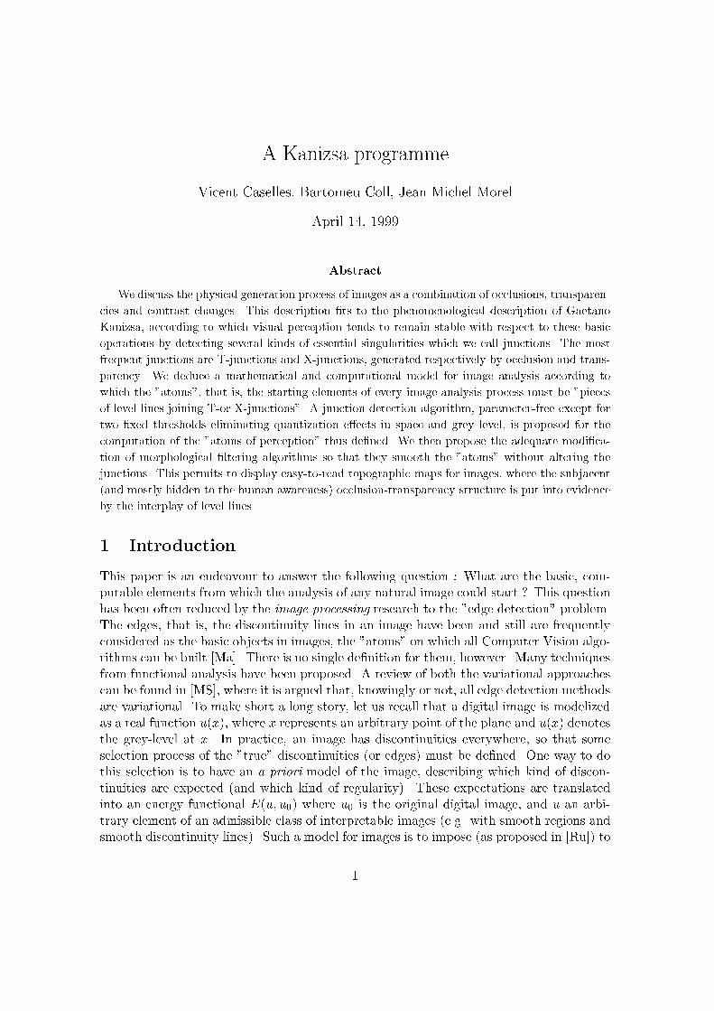
agation. Indeed, frequency, or wavelength, is taken into account in a rather rough wayas colour and the only analogy we can draw between acoustics and image analysis in thisdirection is the way in which new colours are obtained by combining (adding) colourswith di�erent wavelengths. The human perception does that in a very rough manner, sothat colour is taken into account in our understanding of the physical world as a rathersecondary information : think how well we are contented with black and white pictures. Infact, the basic model for image generation is essentially geometric and only assumes thatlight propagates in straight lines, a physically approximately true law. According to thisbasic model, the camera oscura or pinhole model, every point of the surface of physicalobjects re ects solar or arti�cial light in all directions. Generation of images occurs whenthis light is focused by passing through a hole on the side of a black box and �nally im-pressed on the face of the black box opposite to the hole. The black box can be a camera,in which case this face is a photosensitive paper or an array of electronic ampli�ers. Italso is the model of the eye, in which case the photosensitive surface is the retina. (SeeFigure 1).

Calling x a generic point on the retina (or �lm) plane, we call u(x) the result ofthis impression, which we shall throughout this paper assume to be a real value measuringintensity (or energy, or "grey level") of the light sent by x. It is sometimes assumed that thelight sent by the surface of objects is the same in every direction (the so called Lambertianassumption). This assumption is, however, false when mirroring e�ects occur. In fact, itis generally false. Since the repartition of the light sources is not uniform, it is expectedthat di�erent parts of the surface of physically homogeneous objects will re ect di�erentlight intensities. In addition, objects may occult to each other some light sources, so thatshadows appear on their surface. The intricacy of natural images is therefore extreme,and we certainly cannot pretend that images faithfully re ect the objects appearing inthe world. Light sources, shadows, re ectances, apparent contours are the basic visualobjects, more basic for sure than the real objects. Our main concern here is to �nd howthose basic objects can be used to extract physical information on objects from images.In order to do that, we must follow the same method as in acoustics; we must deduce thestructure of the basic objects from the way they have been generated.We shall, following the psychologist and gestaltist Gaetano Kanizsa, de�ne two basicoperations for image generation : occlusion and transparency. In the same way as inacoustics, where the basic operation, the superposition of transient waves, is interpretedas an addition of functions in a Hilbert space, we shall interpret occlusion and transparency

4

as basic operations on images considered as functions u(x) de�ned on the plane.Before beginning with the discussion about geometric operations on images, we wish tomake clear the role which, in our opinion, linear methods should play in image processing.Indeed, we shall reject them in general as image geometric analysis methods. Now, mostoptical devices operate a convolution on the signal and add random perturbations ("noise")to the original image. Thus, most early image processing methods have focused on lineardecomposition methods for image restoration, which is sound since the initial perturbationsalso are linear in a �rst approximation. We shall not adress this matter here and we shallfocus on image analysis methods where either those perturbations are negligible, or havealready been corrected so that we can directly adress the geometric structure of images.

2.1 Occlusion as a basic operation on images

Given an object ~A in front of the camera, we call A the region of the plane to which it cor-responds by the pinhole model, that is, the region it covers on the "retina". We call uA theimage thus generated, which is de�ned in A. Assuming now that the object ~A is added in areal scene ~R of the world whose image was v, we observe a new image which depends uponwhich part of ~A is in front of objects of ~R, and which part in back. Assuming that ~A oc-cludes objects of ~R and is occluded by no object of ~R, we get a new image u ~R[ ~A de�ned by

u ~R[ ~A = uA in A andu ~R[ ~A = v in IR2 nA. (1)

Of course, we do not take into account in this basic model the fact that objects in ~Rmay intercept light falling on ~A, and conversely. In other terms, we have omitted theshadowing e�ects, which will now be considered.

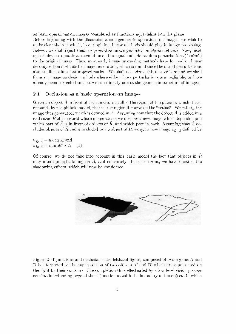
Figure 2. T-junctions and occlusions: the lefthand �gure, composed of two regions A andB is interpreted as the superposition of two objects A' and B' which are represented onthe right by their contours. The completion thus e�ectuated by a low level vision processconsists in extending beyond the T-junction a and b the boundary of the object B', which

5

apparently "stops" when it meets the object A'. This interruption is interpreted as anocclusion.

2.2 Transparency (or shadowing) as a second basic operation on images

Let us assume that the light source is a point in euclidean space, and that an object ~Ais interposed between a scene ~R whose image is v and the light source. We call ~S theshadow spot of ~A and S the region it occupies in the image plane. The resulting image uis de�ned by

u ~R; ~S;g = v in IR2 n S andu ~R; ~S;g = g(v) in S. (2)

Here, g denotes a contrast change function due to the shadowing, which is assumed to beuniform in ~S. Clearly, we must have g(s) � s, because the brightness decreases inside ashadow, but we do not know in general how g looks. The only assumption for introducingg is that points with equal grey level s before shadowing get a new, but the same, grey levelg(s) after shadowing. Of course, this model is not true on the boundary of the shadow,which can be blurry because of di�raction e�ects or because the light source is not reallyreducible to a point. Another problem is that g in fact depends upon the kind of physicalsurface which is shadowed so that it may well be di�erent on each one of the shadowedobjects. This is no real restriction, since this only means that the shadow spot S must bedivided into as many regions as shadowed objects in the scene ; we only need to iterate theapplication of the preceding model accordingly. A variant of the shadowing e�ect whichhas been discussed in perception psychology by Gaetano Kanizsa is transparency. In thetransparency phenomenon, a transparent homogeneous object ~S (in glass for instance) isinterposed between part of the scene and the observer. Since ~S intercepts part of the lightsent by the scene, we still get a relation like (2), so that transparency and shadowing sim-ply are equivalent from the image processing viewpoint. If transparency (or shadowing)occurs uniformly on the whole scene, the relations (2) reduce to

ug = g(v);

which means that the grey-level scale of the image is altered by a nondecreasing contrastchange function g. In natural or arti�cial vision, this happens all the time because so-lar light is constantly changing intensity, being obscured by aerosols or clouds while thelight captors themselves (no matter arti�cial or natural) are subject to drastic sensibilitychanges. There is, however, a di�erence between the change of contrast sensibility of areceptor and a change in the light sources intensity. Indeed, in this last case, the responseof di�erent objects to this change may be di�erent (according to their material) so thatwe may expect that the resulting constrast change g depends upon the objects. Thus, ifthe image domain satis�es

= A1 [A2 [ :::An;

a disjoint union where the Ai denote the visible parts of physically homogeneous objects,then the change of light can be modelized as g = (g1; g2; :::gn), and the new image ug isde�ned from the previous one v by

ujAi= gi(vjAi

): (3)

6

The transparency phenomenon is not restricted to shadows or glass. It occurs with allkinds of spots on objects caused by more or less transparent liquids : water, painting, oil,mud, ink. Since we live in a more and more graphical world, with arti�cial light, we con-stantly see at surfaces (paper, screen, walls) where occlusion and transparency processeshave been repeatedly applied.

Let us mention two more important optical e�ects which increase still more the intri-cacy of natural images (but are naturally included in the transparency-occlusion model):�rst the shading, which makes elements of a homogeneous surface respond in a di�erentway according to their orientation in space. The shading e�ect implies that a homoge-neous object will be visually split into as many parts as facets it has, separated by "edges",that is discontinuity lines due to the sudden changes of orientation of the surface. Thesechanges can also be gradual when the object's surface is smooth. Second phenomenon,the re ectance e�ect, or mirroring e�ect, which makes the surface of some object re ectthe image of other objects or light sources. The extreme case for this phenomenon occurswith mirrors, but most objects present re ectance phenomena. In fact, shading simplymultiplies the number of visual objects (as many as facets of homogeneous objects) andre ectance can be analyzed as a transparency phenomenon. An extreme, but currente�ect of transparency occurs when we look through a glass window : the light comingfrom outsides mixes with the inside light re ected by the window. Calling respectivelyv1, v2 and u the inside image, the outside image and the resulting image, we obtainu = g1(v1) + g2(v2). (Indeed, v1 and v2 are subject to an attenuation (contrast change)respectively due to re ection and transparency.) We may lead back the window e�ect toa transparency phenomenon : It is enough to consider each homogeneous region of v1 asa spot S, inside which the image v2 has been translated in grey level. This correspondsto an extension of our de�nition of transparency. In fact, the resulting image u can bede�ned as a "view of v1 through the inhomogeneous transparent medium v2", and con-versely. The preceding model is compatible with a wide range of transparency phenomena.Transparency- or shadowing-like phenomena are produced in a large variety of physicalsituations: a good example is the case of wetting, which can change the brightness of anyobjects by patches, in the same way as shadows do. This occurs (e.g.) on the groundwhen it is covered with puddles.

2.3 Requirements for image analysis operators

Of course, we do not know a priori, when we look at an image, what are the physicalobjects which have left a visual trace in it. We know, however, that the operations havingled to the actual image are given by formulas (1)-(3). Thus, any processing of the imageshould avoid to destroy the image structure resulting from (1), (2) and (3) : this structuretraduces the information about shadows, facets and occlusions which are clues to thephysical organization of the scene in space. The identity and shape of objects must berecovered from the image by means which should be stable with respect to those operations.As a basic and important example, let us recall how the Mathematical Morphology schoolhas insisted on the fact that image analysis operations must be invariant with respect toany contrast change g. In the following, we shall say that an operation T on an image u

7

is morphological ifT (g(u)) = T (u)

for any nondecreasing contrast change g.

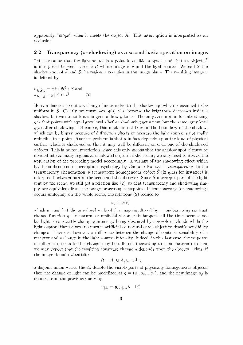
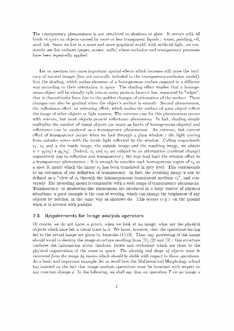
Remark (constrast change and response functions of captors)One of the reasons for which actual contrast changes altering the "true" light intensityare nonlinear is following. Most light captors have a nonlinear behavior and, even worse,have a �nite range. Whenever light is too strong (or too weak), saturation of the captoroccurs. The response function of light captors generally has the shape showed in Figure3.

3 Basic objects of image analysis

We call basic objects a class of mathematical objects, simpler to handle than the wholeimage, but into which any image can be decomposed and from which it can be recon-structed. The classical examples of image decompositions are

� Additive decompositions into simple waves : Basic objects of Fourier analysis are cosineand sine functions, basic objects of Wavelet analysis are wavelets or wavelet packets, basicobjects of Gabor analysis are windowed (gaussian modulated) sines and cosines. In allof these cases the decomposition is an additive one and we have argued against it as notadapted to the structure of images, except for restoration processes. Indeed, operationsleading to the construction of real world images are strongly nonlinear and the simplestof them, the constrast change, does not preserve additive decompositions. If u = u1 + u2,then it is not true that g(u) = g(u1) + g(u2) if the constrast change g is nonlinear.

� Next, we have the representation of the image by a segmentation, that is, a decom-position of the image into homogeneous regions separated by boundaries, or "edges". Thecriterion for the creation of edges or boundaries is the strength of constrast on the edges,along with the homogeneity of regions. Both of these criteria are simply not invariantwith respect to contrast changes. Indeed rg(u) = g0(u)ru so that we can alter the value

8

of the gradient by simply changing the constrast.

� Finally, we can decompose, as proposed by the Mathematical Morphology school, animage into its binary shadows (or level sets), that is, we set X�u(x) = white if u(x) � �and X�u(x) = black otherwise. The white set is then called level set of u. It is easily seenthat, under fairly general conditions, an image can be reconstructed from its level sets bythe formula

u(x) = supf�; u(x) � �g = sup�; x 2 X�u

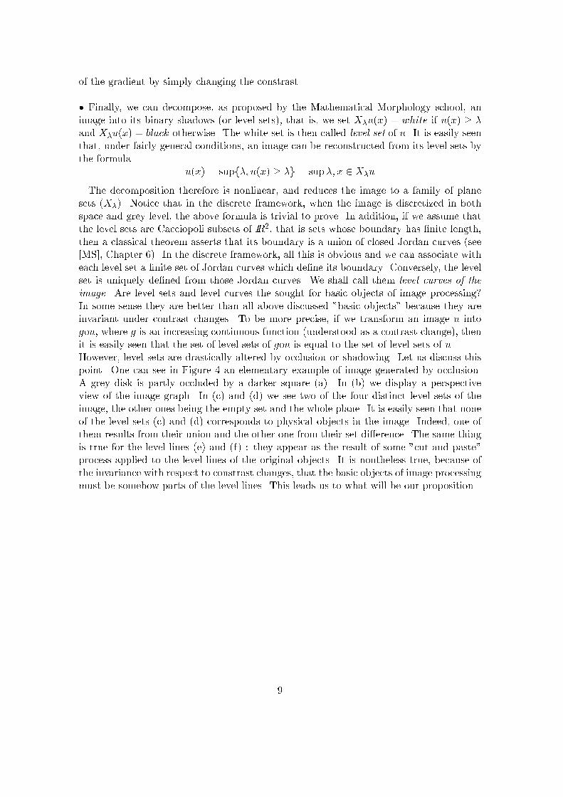
. The decomposition therefore is nonlinear, and reduces the image to a family of planesets (X�). Notice that in the discrete framework, when the image is discretized in bothspace and grey level, the above formula is trivial to prove. In addition, if we assume thatthe level sets are Cacciopoli subsets of IR2, that is sets whose boundary has �nite length,then a classical theorem asserts that its boundary is a union of closed Jordan curves (see[MS], Chapter 6). In the discrete framework, all this is obvious and we can associate witheach level set a �nite set of Jordan curves which de�ne its boundary. Conversely, the levelset is uniquely de�ned from those Jordan curves. We shall call them level curves of theimage. Are level sets and level curves the sought for basic objects of image processing?In some sense they are better than all above discussed "basic objects" because they areinvariant under contrast changes. To be more precise, if we transform an image u intogou, where g is an increasing continuous function (understood as a contrast change), thenit is easily seen that the set of level sets of gou is equal to the set of level sets of u.However, level sets are drastically altered by occlusion or shadowing. Let us discuss thispoint. One can see in Figure 4 an elementary example of image generated by occlusion.A grey disk is partly occluded by a darker square (a). In (b) we display a perspectiveview of the image graph. In (c) and (d) we see two of the four distinct level sets of theimage, the other ones being the empty set and the whole plane. It is easily seen that noneof the level sets (c) and (d) corresponds to physical objects in the image. Indeed, one ofthem results from their union and the other one from their set di�erence. The same thingis true for the level lines (e) and (f) : they appear as the result of some "cut and paste"process applied to the level lines of the original objects. It is nontheless true, because ofthe invariance with respect to constrast changes, that the basic objects of image processingmust be somehow parts of the level lines. This leads us to what will be our proposition.

9

�Our proposition : Basic objects are all junctions of level lines, (particularly: T-junctions, � -junctions, X-junctions, Y-junctions) and parts of level linesjoining them.The terms contained in this proposition will be explicited one by one, starting with T-junctions. We refer to Figure 4 for a �rst simple (but, in fact, general) example. Thelevel lines (e) and (f) represent two level lines at two di�erent levels and in (g) we havesuperposed them in order to put in evidence how they are organized with respect to eachother. We have displayed one of them as a thin line, the other one as a bold line and thecommon part in grey. The T-junctions can be de�ned in such an ideal case as the pointswhere two level curves corresponding to two di�erent levels meet and remain together. Weshall discuss later the other kinds of junctions mentionned above (the above list is anywaynot exhaustive). We shall give below a proposition which justi�es our de�nition of basicobjects. Let us start with some simple phenomenology of junctions.

10

3.1 T-junctions

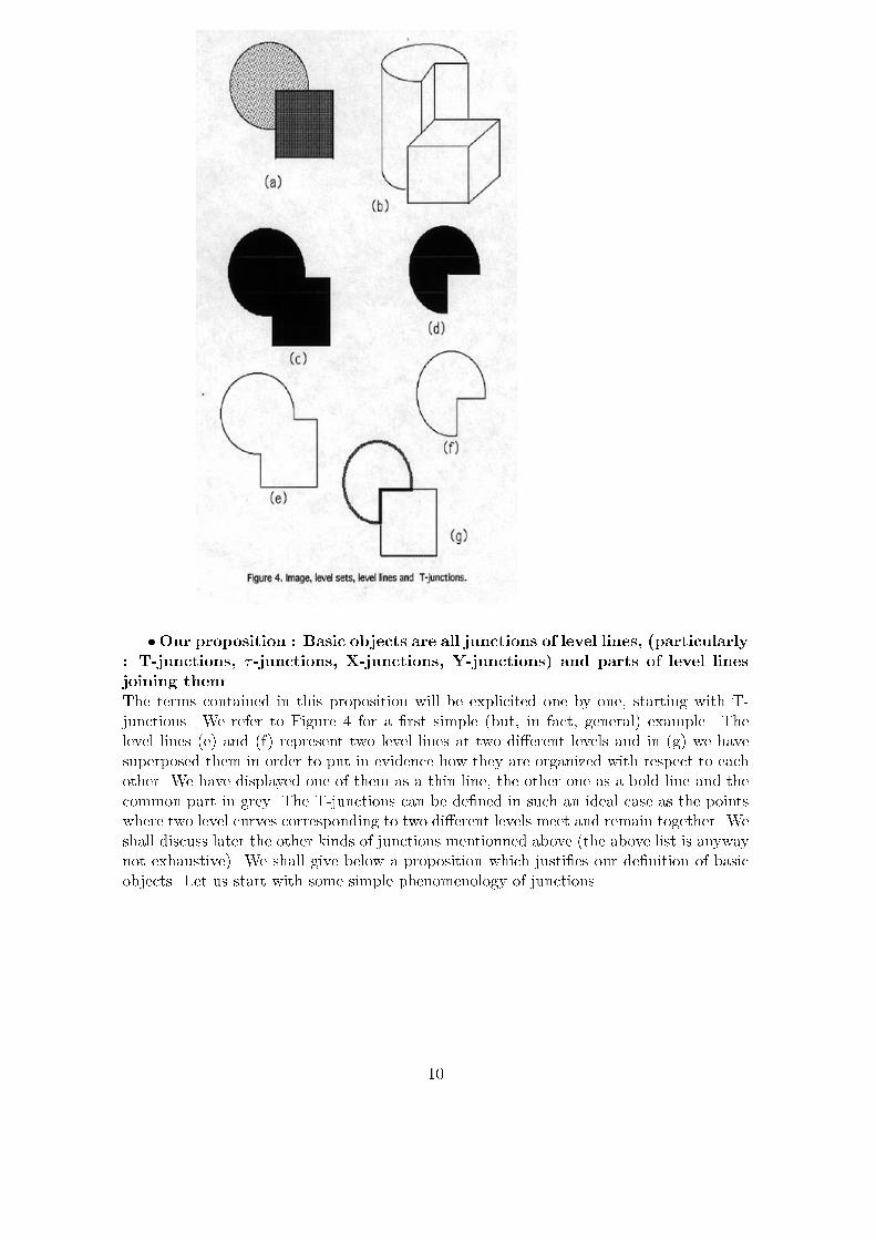
As shown in Figure 5, there are two possibilities which depend upon the order of greylevels around the T-junction. In the �rst case, the T-junction appears as two joint levellines taking at the junction two opposite directions. In the second case, one of the levellines is locally straight and the other one has two branches, one of which coincides withthe �rst level line. Thus a T-junction at a point x can be (a little bit naively) describedin the following way.

� Two level lines meet at point x.

� The half level lines (or branches) starting from x are thus four in number ; two co-incide and two take opposite directions. (The branches which coincide belong to di�erentlevel lines. The branches which take opposite directions may also belong to the same levelline or not).

11

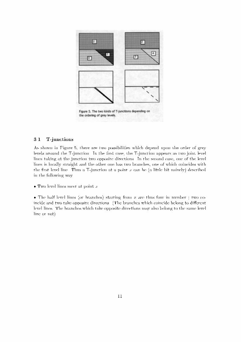
The conditions on the orientation of the branches are absolutely necessary in order todistinguish T-junctions from other phenomena causing the meeting of level lines. Firstof all, the grey level quantization can provoke many meetings of level lines. Figure 6shows this phenomenon for the grey level function u(x; y) = �x � y, where x and ydenote cartesian coordinates after it has been digitized. In principle, the level lines of thisfunction are parallel and never meet. Now, if the grid of discretization has a mesh equalto 1, then successive and should-be-parallel level lines meet at every point of the grid.Another signi�cant example of meeting point for level lines is the case where the imagedisplays the meeting of three facets (and three edges) as displayed in Figure 7. In thiscase, we have a Y-junction, that is, no parallelism between the opposite branches can beobserved.

12

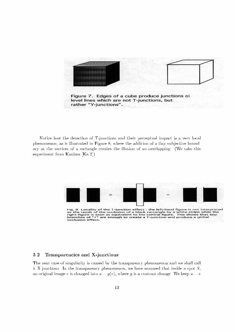
Notice how the detection of T-junctions and their perceptual impact is a very localphenomenon, as is illustrated in Figure 8, where the addition of a tiny subjective bound-ary at the vertices of a rectangle creates the illusion of an overlapping. (We take thisexperiment from Kanizsa [Ka 2]).

3.2 Transparencies and X-junctions

The next case of singularity is caused by the transparency phenomenon and we shall callit X-junctions. In the transparency phenomenon, we have assumed that inside a spot S,an original image v is changed into u = g(v), where g is a contrast change. We keep u = v

13

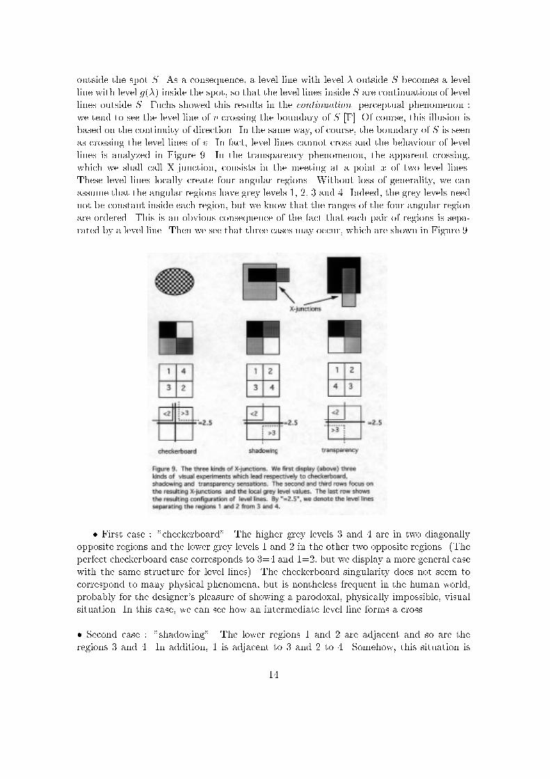
outside the spot S. As a consequence, a level line with level � outside S becomes a levelline with level g(�) inside the spot, so that the level lines inside S are continuations of levellines outside S. Fuchs showed this results in the continuation perceptual phenomenon :we tend to see the level line of v crossing the boundary of S [F]. Of course, this illusion isbased on the continuity of direction. In the same way, of course, the boundary of S is seenas crossing the level lines of v. In fact, level lines cannot cross and the behaviour of levellines is analyzed in Figure 9. In the transparency phenomenon, the apparent crossing,which we shall call X-junction, consists in the meeting at a point x of two level lines.These level lines locally create four angular regions. Without loss of generality, we canassume that the angular regions have grey levels 1, 2, 3 and 4. Indeed, the grey levels neednot be constant inside each region, but we know that the ranges of the four angular regionare ordered. This is an obvious consequence of the fact that each pair of regions is sepa-rated by a level line. Then we see that three cases may occur, which are shown in Figure 9.

� First case : "checkerboard". The higher grey levels 3 and 4 are in two diagonallyopposite regions and the lower grey levels 1 and 2 in the other two opposite regions. (Theperfect checkerboard case corresponds to 3=4 and 1=2, but we display a more general casewith the same structure for level lines). The checkerboard singularity does not seem tocorrespond to many physical phenomena, but is nontheless frequent in the human world,probably for the designer's pleasure of showing a parodoxal, physically impossible, visualsituation. In this case, we can see how an intermediate level line forms a cross.

� Second case : "shadowing". The lower regions 1 and 2 are adjacent and so are theregions 3 and 4. In addition, 1 is adjacent to 3 and 2 to 4. Somehow, this situation is

14

the most stable and least paradoxical of all, since it can be interpreted as the crossingof a shadow line with an edge. It is worth noticing that in this case the level line whichseparates the sets fx; u(x) > 2g and fx; u(x) < 3g can be interpreted indi�erently as theshadow line or the edge line. The other (shadow or edge) line has no existence as a levelline, but is obtained by concatenating two branches of two distinct level lines. The levellines bounding the sets u > 1 and u > 3 only meet at point x and form the "X-junction"which we shall trace in experiments on real images.

� Third case : "transparency". The regions 1 and 2 with lower grey-level and the highergrey-level regions 3 and 4 are again adjacent, but the pairs of extreme regions also areadjacent : 1 to 4 and 2 to 3. The transparent material is adding its own color, which isassumed here to be light grey, so that white becomes light grey and black becomes darkgrey. The interpretation is not twofold in this case : the original edge (horizontal in the�gure) must be the level line bounding the set u > 2. The shadow line (vertical in the�gure), is built with two branches of distinct level lines.

3.3 �-junctions

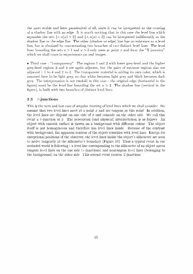
This is the next and last case of singular meeting of level lines which we shall consider. Weassume that two level lines meet at a point x and are tangent at this point. In addition,the level lines are disjoint on one side of x and coincide on the other side. We call thisevent a � -junction at x. The perceptual (and physical) interpretation is as follows. Anobject with smooth surface is shown on a background with di�erent colour. The objectitself is not homogeneous and therefore has level lines inside. Because of the contrastwith background, the apparent contour of the object coincides with level lines. Except forexceptional positions of the observer, the level lines inside the object's silhouette are seento arrive tangently at the silhouette's boundary (Figure 10). Thus a typical event in ouroccluded world is following : a level line corresponding to the silhouette of an object meetstangent level lines on the one side (� -junctions) and nontangent level lines (belonging tothe background) on the other side. This second event creates T-junctions.

15

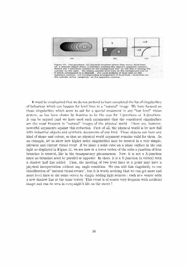
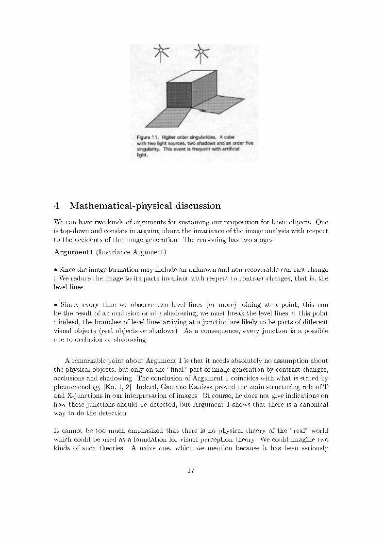
It must be emphasized that we do not pretend to have completed the list of singularitiesof behaviour which can happen for level lines in a "natural" image. We have focused onthose singularities which seem to ask for a special treatment in any "low level" visionsystem, as has been shown by Kanizsa to be the case for T-junctions or X-junctions.It can be argued (and we have used such arguments) that the considered singularitiesare the most frequent in "natural" images of the physical world. There are, however,powerful arguments against this reduction. First of all, the physical world is by now fullwith industrial objects and synthetic documents of any kind. These objects can have anykind of shape and colour, so that no physical world argument remains valid for them. Asan example, let us show how higher order singularities may be created in a very simple,physical and current visual event. If we place a solid cube on a plane surface in the sunlight as displayed in Figure 11, we see how at a lower vertex of the cube a junction of fourbranches is created, like in the transparency phenomenon. Now, it is not a X-junctionsince no branches need be parallel or opposite. In short, it is a Y-junction (a vertex) witha shadow half line added. Thus, the meeting of two level lines at a point may have aphysical interpretation without any angle condition. We can add this singularity to ourclassi�cation of "natural visual events", but it is worth noticing that we can get more andmore level lines at the same vertex by simply adding light sources : each new source addsa new shadow line at the same vertex. This event is of course very frequent with arti�ciallamps and can be seen in everynight's life on the street !

16

4 Mathematical-physical discussion

We can have two kinds of arguments for sustaining our proposition for basic objects. Oneis top-down and consists in arguing about the invariance of the image analysis with respectto the accidents of the image generation. The reasoning has two stages.

Argument1 (Invariance Argument)

� Since the image formation may include an unknown and non recoverable contrast change: We reduce the image to its parts invariant with respect to contrast changes, that is, thelevel lines.

� Since, every time we observe two level lines (or more) joining at a point, this canbe the result of an occlusion or of a shadowing, we must break the level lines at this point: indeed, the branches of level lines arriving at a junction are likely to be parts of di�erentvisual objects (real objects or shadows). As a consequence, every junction is a possiblecue to occlusion or shadowing.

A remarkable point about Argument 1 is that it needs absolutely no assumption aboutthe physical objects, but only on the "�nal" part of image generation by contrast changes,occlusions and shadowing. The conclusion of Argument 1 coincides with what is stated byphenomenology [Ka, 1, 2]. Indeed, Gaetano Kanizsa proved the main structuring role of Tand X-junctions in our interpretation of images. Of course, he does not give indications onhow these junctions should be detected, but Argument 1 shows that there is a canonicalway to do the detection.

It cannot be too much emphasized that there is no physical theory of the "real" worldwhich could be used as a foundation for visual perception theory. We could imagine twokinds of such theories. A naive one, which we mention because it has been seriously

17

considered in Arti�cial Intelligence, would consist in establishing a list of all classes ofexisting objects in the word, with their 3D-shapes and photogrammetry. Now, the realworld's objects are quite diverse! Another way, in order to avoid the never exhausted listof all objects, would be to argue that objects of interest can be generically described, likemathematical objects, as volumes whose boundary is, say, piecewise smooth. Indeed, mostphysical processes tend to create clearcut (and often smooth) objects by crystallization,erosion, fracture and di�usion, while biological processes create lots of piecewise smoothshapes, the same being true for the products generated by the industry.A more attentive re ection, however, (like Benoit Mandelbrot's) reveals that the sameobjects which look smooth at some scale are, when we get closer, composed with smallerobjects which to their turn look smooth, and so on. To take an easy example, we can men-tion the series forest/tree/leaf/limb, an object which has a smooth shape at some scale,then look ragged at an intermediate scale, again recovers a shape at a still smaller scale,etc.. Thus, the fact, asserted with some insistance by psychologists and phenomenologists,that we always see "shapes" with some homogeneity (be it in "texture" or color) and withsmooth boundaries should be considered as a law of perception and not as a faithful de-scription of the Umwelt. So we shall give a perceptual argumentation (and not a physicalone) to complete our preceding Invariance Argument 1. According to the "basic" percep-tual interpretation of the image, which matches (e.g.) all drawings of Gestaltists and thesegmentation algorithms (see [Met], [MS]) :

Argument2 (Based on perception theory) We make the following perceptual assumptions.

� Color constancy principle. Basic perceptual objects are regions with a smooth lumi-nance. Their boundaries are called "apparent contours".

� Genericity of smoothness. Calling u(x) the luminance, we have Du(x) 6= 0 inside eachbasic perceptual object, except at isolated points (which can be extrema or saddle points).

� Occlusion and transparency. The �nal image is obtained by iterating a �nite num-ber of times the processes (1), and (2).

� Genericity of occlusion. Any perceptual object is assumed to have a colour di�erentfrom its background, so that its apparent contours (including its internal apparent con-tours in case of self-occlusion) appear as discontinuity lines of the image. In the same way,shadows are assumed to create discontinuity lines on all objects.

� Regularity of the object's aspects. All apparent contours and shadows have a mini-mal regularity (they have e.g. �nite length).

� Genericity of occlusion and transparency. It is assumed that the level lines of theoccluding, of the occluded and of the shadowed objects are never exactly parallel to theapparent contours or to the contours of the shadow, so that each discontinuity line in theimage meets at almost every point level lines on both sides.

Then, we deduce the following mathematical description of a generic perceptual image

18

:

� We call junction any meeting point of two level lines of the image. Then, inside eachsmoothness region, and except at isolated points (extrema, minima or saddle points), thelevel lines do not meet.

� Each discontinuity line of the image also is a line of bilateral junctions : that is, aline of X-junctions in case of transparency, a line of T-junctions on the one side and � -junctions on the other side in case of occlusion by a smooth object or a line of T-junctionson both sides in case of occlusion by a facet of object.

� As a consequence, shadow spots are de�ned as parts of the image whose boundaryis a Jordan curve of X-junctions and objects are de�ned as the inside part of a Jordancurve of T-junctions.

� Since apparent contours of objects and boundaries of shadow spots are unambigu-ously determined by the lines of junctions, the only pending problem is the classical�gure/background dilemma : given a line of junctions, on which side is the occludingobject and on which side the occluded? This can be only decided if the subjacent physi-cal occluding object has a smooth surface, in which case, the junctions on the occludingobject's side are � -junctions and the junctions on the other side are, by genericity, simpleT-junctions (see Figure 10).

� Let us end with the main consequence : the most basic segmentation of an imagecorresponding to the preceding description is : decomposition of the image into pieces oflevel lines joining junctions, so that we retrieve the conclusion of Argument 1.

As a further remark on Argument 2, we notice that the occluding contours and shadowscan be retrieved in two ways, either by taking advantage of the level lines arrangement,as proposed, or as discontinuity lines of the image. Now, to detect them as discontinuitylines has proved disastrous in the actual technology since digital images are discontinuouseverywhere and we can only de�ne "discontinuity" as a scale-dependent concept. In fact,almost all points are edge points at some scale in a digital image [Wi, Ma] ! In the nextsection, we shall describe the algorithms for extraction of the "basic objects" which followfrom the above discussion.

5 Experimental Kanizsa programme

5.1 Computation of basic visual events

In this section, we discuss how the basic perceptual-physical events discussed above canbe detected in digital images and we present experimental results. The above descriptionof T-, X-, and � -junctions is based on the assumptions that

� Level sets and level lines can be computed.

19

� The meeting of two level lines with di�erent levels can be detected.

� The direction of level lines or level half lines can be de�ned and computed.

� The following events can be numerically implemented : "a branch (half level line) lo-cally coincides with another", "a branch makes an angle with another", "two brancheshave opposite directions", "two branches are tangent".

(Since in practice two level lines with di�erent levels in an image never fully coincide,we see that the last two events involve the computation of a local direction for a branch oflevel line.) In a digital image, the level sets are computed by simple thresholding. A levelset fu(x) � �g can be immediately displayed in white on black background. In the actualtechnology, � = 0; 1; :::; 255, so that we can associate with an image 255 level sets. TheJordan curves limiting the level sets are easily computed by a straightforward algorithm: they are chains of vertical and horizontal segments limiting the pixels. In the numericalexperiments, these chains are represented as chains of pixels by simply inserting" bound-ary pixels" between the actual image pixels. In order to get a correct visual representationof level lines, we therefore apply a zoom with factor 2.We de�ne "junctions" in general as every point of the image plane where two level lines(with di�erent levels) meet. As we have commented in Figure 6, non signi�cant T-junctionsor X-junctions may be observed as a consequence of a gradient large enough in a smoothpart of the image. Assume that the image grid mesh is 1, with a grey level quantized withentire numbers. (In practice, from 0 to 255). Then at points where the gradient is largerthan 1, collapsing of level lines may occur ; it necessarily occurs if the gradient is largerthan

p2. As we shall see in experiments, all constrasted edges present in an image tend

to generate T-junctions if the image is slightly blurry : indeed, the smoothing of an edgegenerates a lot of parallel level lines which collapse at many points, thus generating tinyX-junctions. This fact can be appreciated in image u4 of Experiment 2, where we havedisplayed all junctions, that is, all meetings points between two distinct level lines in animage. As a consequence, the meeting of two level lines can be considered as physicallymeaningful if and only if the level lines diverge signi�cantly from each other. In order todistinguish between the true junctions and the ones due to quantization e�ects, we decideto take into account T-junctions if and only if� the area of the occulting object is large enough,� the apparent area of the occulted object is large enough and� the area of background is large enough too.This threshold on area must be of course as low as possible, because there is a risk toloose T-junctions between small objects. Small size signi�cant objects appear very oftenin natural images : they may simply be objects seen at a large distance. In any case,the area threshold only depends on the quantization parameters of the digital image andtends ideally to zero when the accuracy of the image tends to in�nite. The algorithm forthe elimination of dubious junctions is as follows.

Junction Detection Algorithm

� Fix an area threshold n (in practice, n = 40 pixels seems su�cient to eliminate junctions

20

due to quantization e�ects.)

� Fix a grey level threshold b (in practice : b = 2 is su�cient to avoid grey level quanti-zation e�ects).

� At every point x where two level lines meet : de�ne �0 < �0 the minimum and maximumvalue of u in the four neighboring pixels of x.

� We denote by L� the connected component of x in the set fy; u(y) � �g and by M� theconnected component of x in the set fy; u(y) � �g. Find the smallest � � �0 such thatthe area of L� is larger than n. Call this value �1. Find the largest �; �1 � � � �0, suchthat the area of M� is larger than n. We call this value �1.

� If �1 and �1 have been found, if �1 � �1 � 2b, and if the set fy; �1 � b � u(y) � �1 + bghas a connected component containing x with area larger than n, then retain x as a validjunction.

� (Optional detection of X-junctions) If, in addition, the set fy; �1 � b � u(y) � �1 + bghas a second connected component containing x (meeting the �rst one only at x) witharea larger than n, then retain x as a possible X-junction.

In the experiments, we display the junctions meeting all requirements except the lastone as "T"s and the junctions meeting all requirements, including the last one, as "X"s.The detection of X-junctions must be considered as quite optional and dubious, since itcan be mistaken for the coincidence of two T-junctions on an occluding contour

Computing directions of half level lines and angles between them requires a previous�ltering of the image. The correct �ltering to be done is related to the (AMSS) model([AGLM1]) and will be discussed in Section 6. Let us only mention that the current nu-merical schemes used to solve the PDE based �ltering models mentioned above do notenable us to compute directions and angles between level lines with su�cient accuracy.

5.2 Experiments

The experiments have been made on WorkStation SUN IPC, with an image processingenvironment called MEGAWAVE II, whose author is Jacques Froment.

� Experiment 1 : The boolean structure of occlusion retrieved by level setanalysis in two successive images of a sequence. The eight images u1; :::; u8 of theexperiment are displayed from left to right and from top to bottom. The images u1 andu2 are grey-level images and the other ones are binary images (black and white) whichdisplay level sets and logical operations e�ectuated on them. The coding convention isblack = 0 = false, white = 255 = true, so that we identify level sets with binary im-ages and union with max, intersection with min and set di�erence with "�". We �rstsee el caminante (a walking researcher, photographed by Paco Perales) in two successivepositions u1 and u2. Then el caminante without skirting-board : u3 = fx; u1(x) > 10g

21

and el caminante with skirting-board u4 = fx; u1(x) > 70g. Next, u5 = u4 � u3, thatis, the skirting-board without the walking man, u6 = fx; u2(x) > 70g, El caminante withskirting-board in Position 2. Finally u7 = max(u3; u6) : the resulting black parts displaythe part of the skirting-board occluded in Position 1 plus the part of the ground whichremains occluded by the feet of the caminante in both images. In u8 = min(u7; u5), wedisplay the reconstruction of the whole skirting-board by adding the occluded part in Po-sition 1 deduced from Position 2.

� Experiment 2 : detection of T-junctions as meeting points of level lines. Theoriginal grey-level image is u1. In u2 we see El caminante with skirting-board : u1 > 60and u3 is El caminante without skirting-board. We display in u4 the level lines of u2 inwhite and the level lines of u3 in black with their common parts in dark grey. Candidatesto T-junctions generated by the main occlusions can be seen. They are characterized asmeeting points of a black, a white and a grey line. In u5, we see all T-junctions detectedfrom those two level sets, after a �ltering of spurious T-junctions has been made, witharea threshold n = 80.

� Experiment 3. Transparencies. The criterion for transparency is : a meeting pointof level lines such that the angle between two disjoint pairs of branches is close to �. Theoriginal image u1 displays a transparent plastic ruler superposed to a white paper on theborder of a biological experiment. The next image shows the level lines at two well chosenlevels and the characteristic X-junctions generated by the transparency phenomenon, aspredicted.

� Experiment 4. Transparencies and T-junctions provoked by shadows in asynthetic image. The image u1 is a synthetic image with rendering e�ects (author JoanMontes de Oca). In u2 we display, with the same convention as in Experiments 2 and 3,the level lines at two well chosen levels. One can see an X-junction on the road, due to ashadow and several T-junctions caused by occluding contours. There also is a ��junction,caused by a shadow contour on a cylinder meeting the apparent contour of the cylinder.

� Experiment 5. Choice of the thresholds for the Junction Detection Algo-rithm.As we have argued above, the thresholds n and b should be �xed once for ever, since theyonly attempt to avoid side e�ects of the spatial and grey level quantizations. Now, a toolarge threshold in the Junction Detection Algorithm may eliminate valid junctions. Thefollowing sequence of four images illustrates this fact. All of the four images display theoriginal image El Caminante with (in white) small "T"s indicating locations of detectedjunctions. The original images were 128x128 but for reasons of visualization we displaythem zoomed by a factor 2. Image 5.1 : we take b = 5 and n = 80. Many junctions on theboundary of the image are lost because of the too large choice for b. Image 5.2 : we takeb = 5 and n = 40. This permits more junctions on the well contrasted boundary of theskirting-board, but the low contrasted junctions of the background with the boundary ofthe image remain lost. Image 5.3 : b = 2, n = 40. All physically plausible junctions seemdetected. As expected, the boundary of the image generates an almost continuous line ofjunctions, as well as the main occlusive structures and shadows of the image. Image 5.4 :

22

b = 2 and n = 80. A probably too high area threshold.

� Experiment 6. Transparencies and occlusions in satellite imagingIn this piece of SPOT image (courtesy from CNES), we see the Corsican coast, partiallyoccluded by clouds and partially visible through them. Image 6.1 : b = 2, n = 80. Im-age 6.2 : b = 2, n = 40. Notice how junctions accumulate on the boundaries of cloudsand coasts, while the high-contrasted ground presents very few ones. In these images,T-junctions are denoted by a small white "T" and X-junctions by small white crosses.The crosses are expected to appear at cloudy and shadowy locations of the image.

� Experiment 7. Sensibility to noise The following experiments do not pretend toexhaust the subject of sensibility to noise of the junctions. Image 7.1 (Carretera.img) :original synthetic image (already used in Experiment 4). Images 7.2 and 7.3 : two detailsof the preceding image, which for display reasons we zoomed by a factor 2. The detailimages have 40% of the pixels destroyed and replaced by an uniformly distributed randomvalue between 0 and 255. In white, one can see the obtained T-junctions and X-junctionswith n = 40 and b = 2.

� Experiment 8. Sensibility of T-junctions to blurring. It is important to noticethe relative stability of T-junctions to blurring. The spatial discretization compensatesthe e�ect of blurring by forcing close level lines to meet. Thus, as can appreciated in thisexperiment, a perfect T-junction blurred by a wide Gaussian can be anyway detected, butits position is altered. Image 8.1 is a 128*128 original perfect T-junction image convolvedwith a gaussian with a 10 pixels standard deviation. Image 8.2 displays all found junc-tions, b = 2 and n = 40. Notice how the original junction has split into several ones andnotice also the displacement of the junction. Images 8.3 displays two characteristic pairsof level lines generating junctions of 8.2. Image 8.4 : All level lines of a detail of Image 7.1,already exploited in Experiment 7. This permits to appreciate how, even in a syntheticimage, the blurring due to spatial quantization provokes a doubling of certain occlusionboundaries and, when the boundary is straight and parallel to the grid, we obtain spuriousT-junctions. .

6 Image �ltering preserving Kanizsa singularities

6.1 Image and level curve smoothing models

In this section, we push a little further the exploration of invariant image or level lines�ltering methods which have been recently proposed in [AGLM 1, 2] and [ST 1,2]. Accord-ing to the axiomatic presentation of image iterative smoothing (or "pyramidal �ltering",or "scale space") proposed in [AGLM2], all iterative �ltering methods, depending on ascale parameter t, can be modelized by a di�usive partial di�erential equation of the kind

@u

@t(t; x; y) = F (D2u(t; x; y);Du(t; x; y); x; y; t); u(0; x; y) = u0(x; y);

where u0(x; y) is the initial image, u(t; x; y) is the image �ltered at scale t and Du;D2u de-note the �rst and second derivatives with respect to (x; y). (We setDu(x; y) = (@u

@x(x; y); @u

@y(x; y)) =

23

(ux; uy)(x; y) and in the same way, we de�ne D2u(x; y) as the symmetric matrix of secondpartial derivatives uxx; uxy; uyx; uyy of u with respect to x and y.)

The most invariant "scale space" proposed in [AGLM1], is the A�ne MorphologicalScale Space, that is, an equation of the preceding kind which is invariant with respect tocontrast changes of the image and a�ne transforms of the image plane,

(AMSS)@u

@t= jDuj(curv(u)) 13 ; u(0; x; y) = u0(x; y);

where

curv(u)(x; y) =uxx(uy)

2 � 2uxyuxuy + uyy(ux)2

(u2x + u2y)3

2

(x; y)

is the curvature of the level line passing by (x; y). The interpretation of the AMSS model isgiven in [AGLM1] and corresponds to the following evolution equation for curves, proposedindependently in [ST1] and which we call (ASS) (A�ne Scale Space of curves)

(ASS)@C

@t(t; s) = (curv(C(t; s)))

1

3~n(t; s); C(0; s) = C0(s);

where C(0; s) is an initial curve embedded in the plane and parameterized by s, ~n(t; s) isthe normal unit vector at C(t; s) and curv(C(t; s)) the curvature of the curve at C(t; s).The relation between (AMSS) and (ASS) is formally the following : (AMSS) moves alllevel lines of u(t; x; y) as if each one were moving by (ASS). At the mathematical level,however, existence and uniqueness results are not at the same stage. (AMSS) has beenproved to have a unique solution in the viscosity sense when the initial image is continuous.(ASS) is proved so far to have a unique smooth solution when the initial curve is convex[ST2]. The main drawback of the classi�cation proposed in [AGLM1] is the (necessary)assumption that the initial image u0(x) is continuous with respect to x. Without thisassumption, the (AMSS) model and the related morphological models loose mathematicalconsistency. This drawback can be avoided by using the Osher-Sethian [OS] method : Ifwe wish to apply (AMSS) to (e.g.) a binary and therefore discontinuous image �X , wesubstitute to �X the signed distance function u0 to X, which is Lipschitz and has X aszero level set : X = fx; u0(x) � 0g. We apply to u0 the (AMSS) model and de�ne theevolution of X as the zero level set of u(t). Evans and Spruck [ES] have shown that suchan evolution does not depend upon the chosen distance function and coincides with (ASS)when the evolution of the boundary of X is well de�ned and smooth. In other terms,we can use (AMSS) either for moving continuous functions, or for moving a single set,or a single Jordan curve, by moving its distance function. In order to deal with generaldiscontinuous functions, we deduce that the (AMSS) evolution will be well de�ned only ifwe can reduce it to the joint motion of single level curves.

6.2 A Kanizsa model for image evolution

Here, we refer to our discussion on the basic objects of Image Analysis, in Section 3.According to this discussion, the decomposition of u0 into its level lines followed by afurther independent analysis of each is not correct : indeed, level lines interact at allimage singularities (T-, X-junctions,... ) and we have argued that atoms of the imagemust be the pieces of level lines joining junctions and not the level lines themselves. In

24

other terms, a correct atomic decomposition of the image implies a previous segmentationof the level lines. After this segmentation only, the smoothing described by (AMSS)or (ASS) can be applied. This means that we are allowed to move the level lines (forsmoothing, or multiscale analysis purposes) but with internal boundary conditions : thelevel lines being during their motion constrained to pass by their endpoints, the junctions.The image model which arises from the preceding discussion is following.

De�nition(Kanizsa image model)We call image a function u(x) whose level lines have all a �nite length and meet only ona closed set without interior Z, which we call the set of junctions of u.

When the junction set is �nite (which is the case for digital images), we set Z =fz1; z2; :::; zng. According to the preceding discussion, the correct adaptation of the(AMSS) model to images having junctions is

Algorithm 1 : Junctions-preserving, a�ne invariant and contrast invariantsmoothing� Compute the junctions z1; z2; :::; zn (by the Junction Detection algorithm, which is a�neinvariant).

� Move each piece of level curve C by the (ASS) model. If the curve has endpoints,they remain �xed and the (ASS) evolution is not allowed to let the curve cross otherjunctions. This yields C(t).

� Reconstruct a smoothed image u(t; x; y) which has the curves C(t) as level lines andthe zi as junctions. This reconstruction is possible because the (ASS) model preserves theinclusion of curves (see [AM])

Let us give a variant of the preceding algorithm which permits a progressive removalof junctions (according to their scale).

Algorithm 2 : progressive removal of junctionsFor every t, starting from t = 0:� Compute the junctions z1; z2; :::; zn (by an a�ne invariant algorithm).

� Move each piece of level curve C by the (ASS) model, as speci�ed in Algorithm 1.This yields C(t).

� Remove at scale t all junctions which do not meet anymore the requirements of theJunction Detection Algorithm with respect to the new level curves C(t).

� Reconstruct a smoothed image u(t; x; y) which has the curves C(t) as level lines andthe remaining zi as junctions.

In the next subsubsection, we shall discuss how to implement Algorithm 1, Algorithm

25

2 being a variant including in its loop the Junction Detection Algorithm.

6.2.1 Mathematical and numerical discussion of Algorithms 1, 2

Both algorithms (1 and 2) are well de�ned provided the (ASS) model is mathematicallycorrectly posed ; this point is, however, still not completely solved. In addition, theindependent processing of all pieces of level lines looks computationally heavy. So weprefer to consider a variant of (AMSS) implementing Algorithms 1 and 2. We considerthe characteristic function �Z(x; y) = 0 if (x; y) 2 Z and �Z(x; y) = 1 if (x; y) =2 Z of thejunctions and apply to the original image the equation

(AMSS1)@u

@t= �Z(x; y)jDuj(curv(u))

1

3 ; u(0; x) = u0(x):

We conjecture that such an equation makes sense, and has a unique viscosity solution(in the sense de�ned in [CIL]) preserving the singularities and moving each piece of levelline by the (ASS) model. In addition, we conjecture that the pieces of level lines joiningjunctions keep the same endpoints by such a process. We shall discuss in the next sectionin which way well-posedness can be proved for (AMSS1).

Let us now consider a well-posed approximation of (AMSS1). We replace �Z by afunction �Z;" which is smooth (e.g. C1) and satis�es

�Z;"(x; y) = 1

if the distance of (x; y) to Z is larger than " and

�Z;"(x; y) = 0

if the distance of (x; y) to Z is smaller than "2and 0 � �Z;" � 1 everywhere. This function

simply is a smooth approximation of the characteristic function of Z, �Z , for which we candirectly apply known existence and uniqueness theorems. The considered model thereforeis

(AMSS")@u

@t= �Z;"(x; y)jDuj(curv(u))

1

3 :

and it is an equation of the kind

@u

@t(t; x; y) = F (D2u(t; x; y);Du(t; x; y); x; y); u(0; x; y) = u0(x; y);

where F is continuous with respect to all variables, nondecreasing with respect to its �rstargument and satisfying the condition

(4) 8x 2 IR2; F (0; 0; x) = 0;

and some additional continuity conditions for F which are easily checked in our case. Then,as it is proved in [GGIS], (AMSS") has a unique solution in the viscosity sense. Therefore,it also satis�es a local comparison principle. Indeed, by Theorem 4.2 in [GGIS], we have acomparison principle between sub- and supersolutions of (AMSS"). Moreover, because of

26

(4), constant functions are solutions of (AMSS"), and, as in [CGG] Theorem 4.5, by using[CGG] Proposition 2.3 and the comparison principle mentioned before, one can constructby the Perron method a (unique) viscosity solution for (AMSS"). In this argument, wehave assumed that the image is de�ned in all of IR2. This does not matter, since we canimpose without loss of consistency in our model that all points on the boundary of ourimage are T-junctions. Then the image can be extended by 0 to the whole plane. Anotherpoint to make clear in the application of the above theorems is following : the existenceand uniqueness results apply only if the initial datum u0 is continuous, which is not ourcase. So we can argue in the following way. Let us call Z" the "-neighborhood of Z.We know that outside Z "

2

the function u0 is continuous. So we can, by Tietze Theorem,extend u0 inside Z "

2

as a continuous function, which we call ~u0. Then the existence anduniqueness theorems mentioned above apply. It only remains to prove that the solutionthus obtained does not depend upon the choice of the extension ~u0. Indeed, it is easilyseen that inside Z "

2

solutions of (AMSS") with continuous initial data does not move. Wededuce, as an easy consequence of the comparison principle, that all continuous extensionsof u0 inside Z "

2

yield the same solution outside.

The interpretation of (AMSS") is essentially the same as for (AMSS1) : the level linesof u with endpoints on Z are constrained to keep the same endpoints and the only di�er-ence with respect to AMSS1 is an alteration of their speed in an "-neighborhood of Z. Ofcourse, it is more than likely that the solution of (AMSS") converges to the (to be proved)solution of (AMSS1), which is the right model. We conjecture that this convergence istrue and we can give hints in the next subsection about existence for (AMSS1) which alsosuggest in which sense this convergence can be true. Returning to (AMSS"), we wouldlike to make clear that it is in fact the right model for what we can numerically implement.Any numerical implementation of (AMSS1) is done on a grid and derivatives of u at apixel (x; y) computed with the neighbooring pixels. We refer to [AM] where a very easyand most invariant such numerical scheme (due to Luis Alvarez and Frederic Guichard) isproposed for (AMSS). The only alteration which we do for this scheme is following : If(x; y) is a vertex of the grid belonging to Z, we simply �x in the scheme the four pixelssurrounding (x; y). In other terms, we call un the successive discretized values of un andwrite the Alvarez-Guichard scheme for (AMSS") in the form

un+1(x; y) = un(x; y) + �tF (D2un(x; y);Dun(x; y); (x; y));

where of course (x; y) are discrete values and �t a small enough time (or scale) increment.Then the new scheme, associated with (AMSS") simply is

un+1(x; y) = un(x; y) + �tF (D2un(x; y);Dun(x; y); (x; y))

if (x; y) are the coordinates of a pixel not touching a T � junction, and

un+1(x; y) = un(x; y)

otherwise. This slight change in the scheme has dramatic consequences in the evolutionof the image in scale space, as we shall see in the numerical experiments.

27

6.3 Experiments in junction-preserving image �ltering

� Experiment 9. Image �ltering preserving Kanizsa singularities. Image 9.1 :(AMSS), applied to the synthetic image 7.1 without �xing the junctions : those junctionsare then considered as points with high curvature (angles, in fact) and therefore rounded.The image corresponds to t = 6. See how the white stripe on the road which was shad-owed disappears much faster than the other ones. Image 9.2 : Detected junctions (n = 40,b = 5). Image 9.3 : Algorithm 1 applied to Image 7.1. More precisely :(AMSS) �ltering ofImage 7.1 at scale t = 6, with all junctions displayed in Image 9.2 �xed. Compare to 9.1 :The geometry of the image is essentially maintained. Incidentally, the junction detectionalgorithm has detected several angles on the white stripes. This is due to blurring e�ectsof the spatial quantization, which doubled some of the stripes boundaries. Noticeable ishow "unnatural" this synthetic image behaves under certain aspects : A natural imagewould have many junctions at all occlusive boundaries, because no background is reallycompletely uniform. Here, instead, the grey levels of the road and of the stripes is simplyconstant; as a consequence, the fact that the white stripes are occluding objects are notsystematically detected.

� Experiment 10. Image �ltering preserving Kanizsa singularities in presenceof noise. Image 10.1 : Same as 7.2 , described above. Image 10.2 : (AMSS) �ltering ofImage 10.1 at scale t = 12. Image 10.3 : Algorithm 1 applied to Image 10.1 at the samescale t = 12.

� Experiment 11. Image �ltering preserving Kanizsa singularities on a realimage. This is essentially the same experiment as Experiments 9 and 10, but done witha "natural" image. Image 11.1 : the original image El caminante, already analysed in Ex-periment 5, after a zoom with factor 2. Images 11.2 and 11.3 : (AMSS) analysis at scalest = 3; 12. Images 11.4 and 11.5 : Algorithm 1, at the same scales. (The �xed junctions arethose obtained in Image 5.3, with area threshold n = 40 and contrast threshold b = 2).

� Experiment 12. Topographic maps. The application of Algorithm 1 simpli�esthe shape of level lines and permits to better visualize the whole topographic organizationof level lines and junctions (that is, all of the proposed "atoms" for image analysis). Image12.1 : original level lines of Image 11.1 displayed for all even levels, 2, 4, 6, etc. Images12.2 and 12.3 show the same level lines of Images 11.4 and 11.5, respectively. Image 12.4:level lines of Image 11.5, but displaying only the level lines for levels which are multiplesof 5.

� Experiment 13. Topographic maps. Same experiment as Experiment 12 applied tothe DNA image already considered in Experiment 3. Image 13.1 : original image whichis the same as Image u1 of Experiment 3 after a zoom with factor 2. Image 13.2: levellines of Image 13.1, with all levels which are multiples of 5. We then apply the JunctionDetection Algorithm with b = 2, n = 20. The area threshold, lower as usual, is necessi-tated by the thin structures in this image, which are borderline in the sense that the sizeof the blurring kernel is close to the size of the thin structures. If we apply a larger areathreshold, some structures are lost. Image 13.3: Algorithm 1 applied to Image 13.1 at the

28

scale t = 12. Images 13.4, 13.5, 13.6 : level lines of Image 13.3 for levels multiples of 5, 10and 20, respectively.

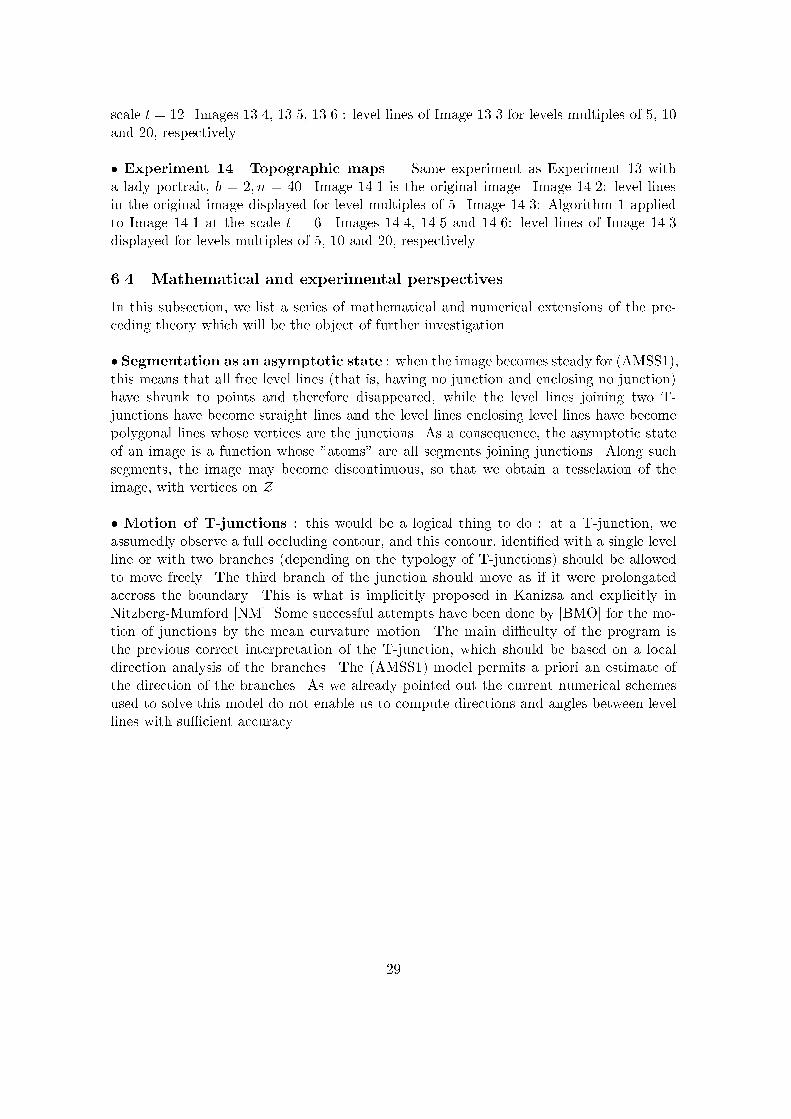
� Experiment 14. Topographic maps. Same experiment as Experiment 13 witha lady portrait, b = 2; n = 40. Image 14.1 is the original image. Image 14.2: level linesin the original image displayed for level multiples of 5. Image 14.3: Algorithm 1 appliedto Image 14.1 at the scale t = 6. Images 14.4, 14.5 and 14.6: level lines of Image 14.3displayed for levels multiples of 5, 10 and 20, respectively.

6.4 Mathematical and experimental perspectives

In this subsection, we list a series of mathematical and numerical extensions of the pre-ceding theory which will be the object of further investigation.

� Segmentation as an asymptotic state : when the image becomes steady for (AMSS1),this means that all free level lines (that is, having no junction and enclosing no junction)have shrunk to points and therefore disappeared, while the level lines joining two T-junctions have become straight lines and the level lines enclosing level lines have becomepolygonal lines whose vertices are the junctions. As a consequence, the asymptotic stateof an image is a function whose "atoms" are all segments joining junctions. Along suchsegments, the image may become discontinuous, so that we obtain a tesselation of theimage, with vertices on Z.

� Motion of T-junctions : this would be a logical thing to do : at a T-junction, weassumedly observe a full occluding contour, and this contour, identi�ed with a single levelline or with two branches (depending on the typology of T-junctions) should be allowedto move freely. The third branch of the junction should move as if it were prolongatedaccross the boundary. This is what is implicitly proposed in Kanizsa and explicitly inNitzberg-Mumford [NM]. Some successful attempts have been done by [BMO] for the mo-tion of junctions by the mean curvature motion. The main di�culty of the program isthe previous correct interpretation of the T-junction, which should be based on a localdirection analysis of the branches. The (AMSS1) model permits a priori an estimate ofthe direction of the branches. As we already pointed out the current numerical schemesused to solve this model do not enable us to compute directions and angles between levellines with su�cient accuracy.

29

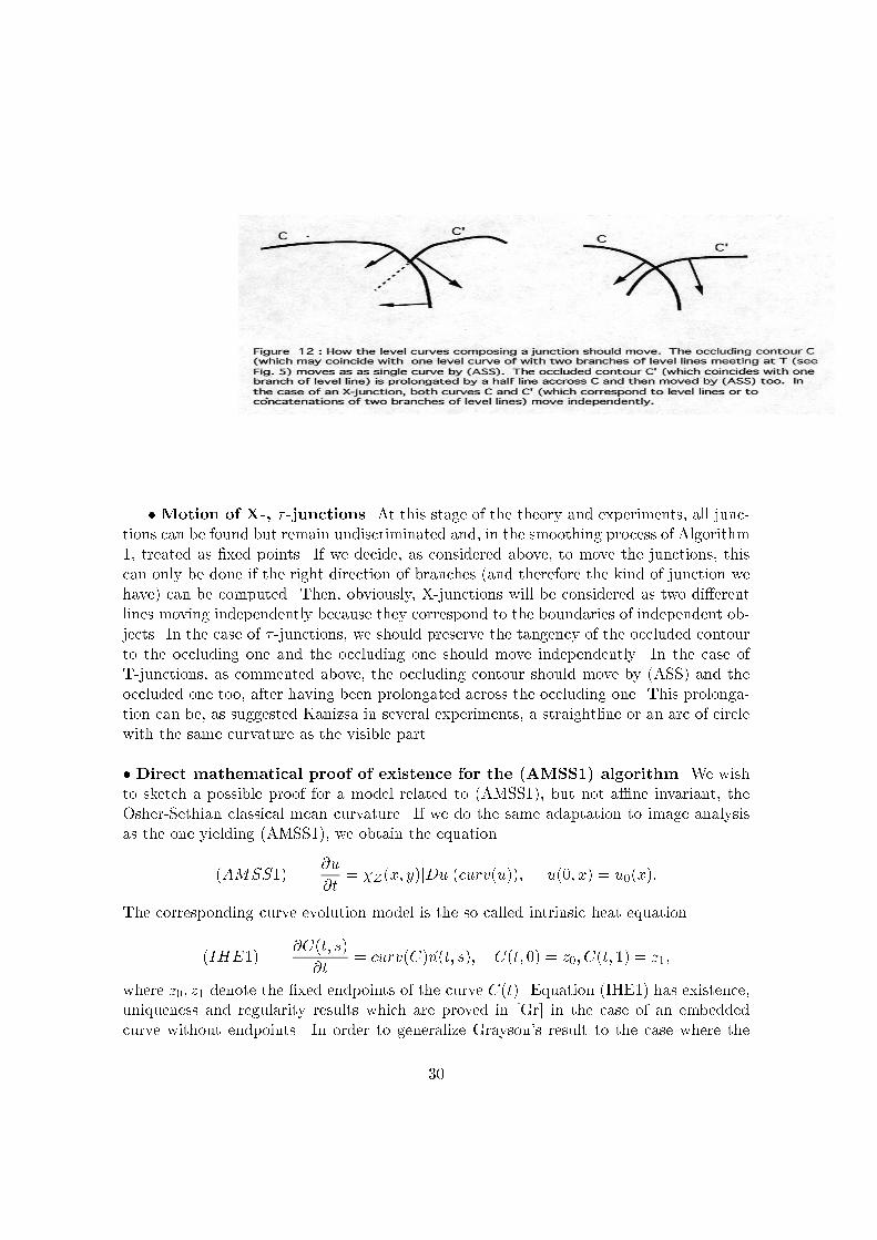
�Motion of X-, � -junctions. At this stage of the theory and experiments, all junc-tions can be found but remain undiscriminated and, in the smoothing process of Algorithm1, treated as �xed points. If we decide, as considered above, to move the junctions, thiscan only be done if the right direction of branches (and therefore the kind of junction wehave) can be computed. Then, obviously, X-junctions will be considered as two di�erentlines moving independently because they correspond to the boundaries of independent ob-jects. In the case of � -junctions, we should preserve the tangency of the occluded contourto the occluding one and the occluding one should move independently. In the case ofT-junctions, as commented above, the occluding contour should move by (ASS) and theoccluded one too, after having been prolongated across the occluding one. This prolonga-tion can be, as suggested Kanizsa in several experiments, a straightline or an arc of circlewith the same curvature as the visible part.

� Direct mathematical proof of existence for the (AMSS1) algorithm. We wishto sketch a possible proof for a model related to (AMSS1), but not a�ne invariant, theOsher-Sethian classical mean curvature. If we do the same adaptation to image analysisas the one yielding (AMSS1), we obtain the equation

(AMSS1)@u

@t= �Z(x; y)jDuj(curv(u)); u(0; x) = u0(x):

The corresponding curve evolution model is the so called intrinsic heat equation

(IHE1)@C(t; s)

@t= curv(C)~n(t; s); C(t; 0) = z0; C(t; 1) = z1;

where z0; z1 denote the �xed endpoints of the curve C(t). Equation (IHE1) has existence,uniqueness and regularity results which are proved in [Gr] in the case of an embeddedcurve without endpoints. In order to generalize Grayson's result to the case where the

30

tips of the curve are �xed, one may proceed as follows. Assuming that the initial curveC0(s) is parameterized by a parameter s ranging from 0 to 1, we embed C0 into a periodiccurve by setting

~C(s) = C(0)� C(�s) if � 1 � s � 0

and then by embedding ~C into a 2-periodic curve. If, by this process, ~C has remained asimple curve (a curve without self-intersection), then we can apply the main theorem in[Gr] and assert that ~C(t; s) is uniquely de�ned, independent of the initial parameterization,and analytic for every t > 0. In addition, because of the uniqueness of the evolution, ~C(t; s)is equal to the curve obtained by evolving C0(�s). Thus ~C is invariant by the symmetryx! �x in IR2, so that z0 belongs to ~C for every t. In the same way, z1 belongs to ~C andwe de�ne the solution of (IHE1) as the part of ~C joining z0 and z1. In the case where ~C0

does present self-intersections, we conjecture that the Grayson proof applies anyway, sincethe self-intersections happen between parts of the curve belonging to di�erent periods andcannot create singularities. It is therefore very likely that these self-intersections disappearafter a while and the curve tends to a straight line joining z0 and z1 as t!1. We do thesame conjecture for the equation

(ASS1)@C

@t= (curv(C))

1

3~n(t; s); C(t; 0) = z0; C(t; 1) = z1;

with the di�erence that the convergence to the straight line should take a �nite time.

6.5 Relation with the Nitzberg and Mumford 2.1-D sketch

In this subsection, we adress the problem of how to use the information on junctionsprovided by our method in order to obtain faithful information on the ordering in spaceof the objects in an image. The only theory to adress this question in its full complexityis, according to our knowledge, the Nitzberg-Mumford "2.1-D sketch". Let us start witha description of this theory [NM]. It is presented as a variant of the Mumford and Shahsegmentation model allowing regions to overlap. If a region occludes another, this can beinterpreted as a \depth" information: one of the objects is in front and the other in back.The information structure obtained by the Nitzberg and Mumford method is mainly two-dimensional (a partition of the images into regions, a segmentation). Now, it also yields apartial ordering of regions in space; for any pair of regions we know which region is in frontand which in back. Therefore the name of \2.1" sketch is an intermediate one betweenthe merely 2D segmentation and to the \2.5-D sketch" of David Marr. (The 2.5-D sketchaimed at a faithful quantitative reconstruction of the spatial environment.)

The data structure proposed by Nitzberg and Mumford consists in regions Ri in thedomain D of the image corresponding to the distinct objects Oi in front of the lens wherethe Ri are partially ordered by occlusion between the objects Oi and where the parts ofthe objects Oi behind other Ojs are reconstructed, so that the Ris overlap. In order tocompute this data structure, they seek a decomposition of D into overlapping orderedregions fRig such that

a) The intensity of the image on the visible part of each Ri is as constant as possible.

31

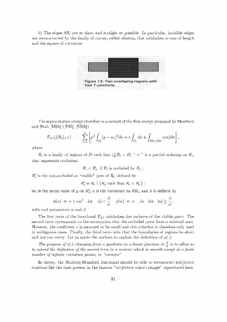
b) The edges @Ri are as short and straight as possible. In particular, invisible edgesare reconstructed by the family of curves, called elastica, that minimizes a sum of lengthand the square of curvature.

The segmentation energy therefore is a variant of the �rst energy proposed by Mumfordand Shah [MSh] ([NM], [NMS])

E2:1(fRig; <) ==nXi=1

"�2ZR0

i

(g �mi)2dx+ "

ZRi

dx+

Z@Rin@D

�(�)d�

#;

where

Ri is a family of regions of D such thatSiRi = D; \ < " is a partial ordering on Ri,

that represents occlusion:

Ri < Rj if Ri is occluded by Rj ;

R0i is the non-occluded or \visible" part of Ri, de�ned by

R0i = Ri n fRj such that Ri < Rjg ;

mi is the mean value of g on R0i; � is the curvature on @Ri, and � is de�ned by

�(�) = � + ��2 for j�j < �

��(�) = � + �� for j�j � �

�:

with real parameters � and �.

The �rst term of the functional E2:1 minimizes the variance of the visible parts. Thesecond term corresponds to the assumption that the occluded parts have a minimal area.However, the coe�cient � is assumed to be small and this criterion is therefore only usedin ambiguous cases. Finally, the third term asks that the boundaries of regions be shortand not too curvy. Let us quote the authors to explain the de�nition of �(�):

The purpose of �(�) changing from a quadratic to a linear function at �� is to allow us

to extend the de�nition of the second term to a contour which is smooth except at a �nitenumber of in�nite-curvature points, or \corners".

In theory, the Nitzberg-Mumford functional should be able to reconstruct subjectivecontours like the ones present in the famous "subjective white triangle" reproduced here.

32

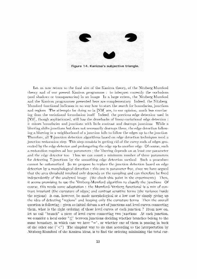
Let us now return to the �nal aim of the Kanizsa theory, of the Nitzberg-Mumfordtheory and of our present Kanizsa programme : to interpret correctly the occlusions(and shadows or transparencies) in an image. In a large extent, the Nitzberg-Mumfordand the Kanizsa programmes presented here are complementary. Indeed, the Nitzberg-Mumford functional indicates in no way how to start the search for boundaries, junctionsand regions. The attempts for doing so in [NM] are, to our opinion, much less convinc-ing than the variational formulation itself. Indeed, the previous edge detection used in[NM], though sophisticated, still has the drawbacks of linear-variational edge detection :it misses boundaries and junctions with little contrast and destroys junctions. While ablurring shifts junctions but does not necessarily destroys them, the edge detection follow-ing a blurring in a neighborhood of a junction fails to follow the edges up to the junction.Therefore, all T-junction detection algorithms based on edge detection techniques need ajunction restoration step. This step consists in getting rid of the curvy ends of edges gen-erated by the edge detector and prolongating the edge up to another edge. Of course, sucha restoration requires ad hoc parameters ; the blurring depends on at least one parameterand the edge detector too. Thus we can count a minimum number of three parametersfor detecting T-junctions by the smoothing edge detection method. Such a procedurecannot be automatized. So we propose to replace the junction detection based on edgedetection by a morphological detection : this one is parameter free, since we have arguedthat the area threshold involved only depends on the sampling and can therefore be �xedindependently of the analyzed image. (We check this point in the experiments). Then,it seems promising to use the Nitzberg-Mumford algorithm to classify the junctions. Ofcourse, this needs some adaptation : the Mumford-Nitzberg functional is a mix of con-trast invariant (the curvature of edges) and contrast sensitive terms (the variance insidethe regions). It can, however, be made morphological at a low cost by simply giving upthe idea of detecting "regions" and keeping only the curvature terms. Then the overallquestion is following : given as initial datum a set of junctions and level curves connectingthem, what is the right ordering of those level curves at each junction ? From now on,let us call "branch" a piece of level curve connecting two junctions. At each junction,we consider a local order "�" between junctions deciding whether branches belong to thesame boundary, in which case we have "=", or whether one of them is passing in backof the other one ("<"). The simplest way to do that according to the interpretation byNitzberg-Mumford of the Kanizsa ideas, is to �nd the ordering minimizing the total cur-

33

vature, an occluded branch being counted without angle, since it is assumed to continuestraight in its occcluded part. This simpli�es a lot the Nitzberg-Mumford idea and makesit parameter free and local : Here is how a rough 2.1 sketch should work according to thepreceding discussion.

Rough 2.1 Sketch Algorithm� Compute all junctions and level lines by the algorithm described in Subsection 4.1.� Apply (AMSS1) to compute the directions of branches at junctions.� At each junction and using the angles of branches delivered by the preceding step : com-pute the arrangement of branches which yields minimal curvature. This would answer thefollowing question: if the junction has three branches : is it a T- or a � or a Y-junction?If the junction has four branches, is it an X-junction ?

Another possibility for developing a (more orthodox) 2.1 sketch from the preceding con-siderations is to do a region growing algorithm where the merging of two regions is madeif and only if the Nitzberg-Mumford energy decreases. The mathematically soundness ofsuch a procedure is discussed in [MS]. The Kanizsa programme solves the problem of theinitial condition for such a merging : the initial boundaries should be all level lines con-necting two T-junctions, and the initial regions the connected components of the imagewhen those level lines are removed.

Acknowledgement. We gratefully acknowledge partial support by EC Project "Mathemat-ical Methods for Image Processing", reference ERBCHRXCT930095, DGICYT project,reference PB94-1174 and CNES. Also, we thank Jean Petitot, Bernard Teissier, MarcellaMairota, Denis Pasquignon, Jacques Froment, Jean-Pierre d'Ales, Antonin Chambolle andFr�ed�eric Guichard for valuable information and discussions.

34

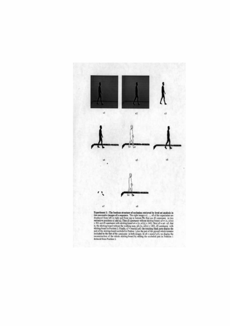
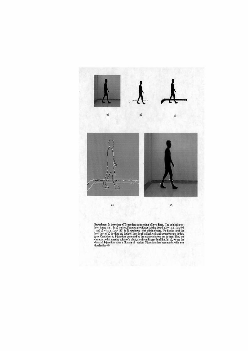
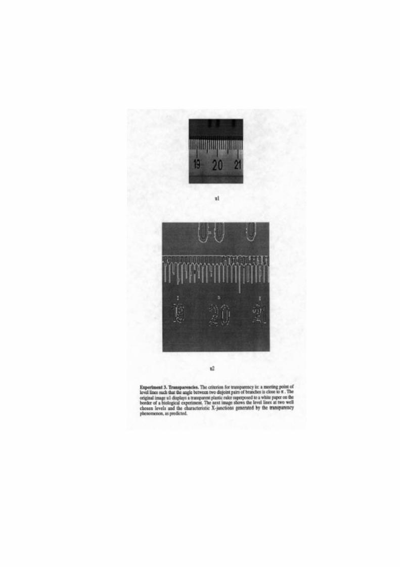
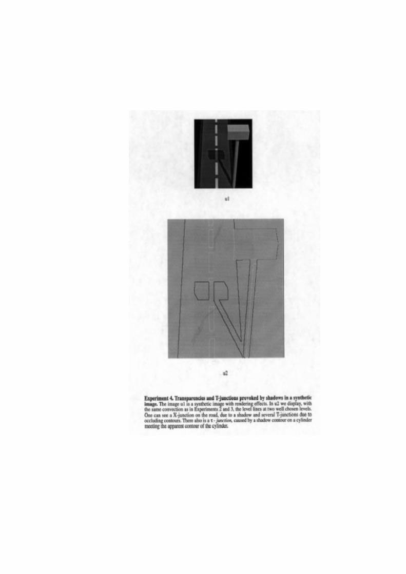
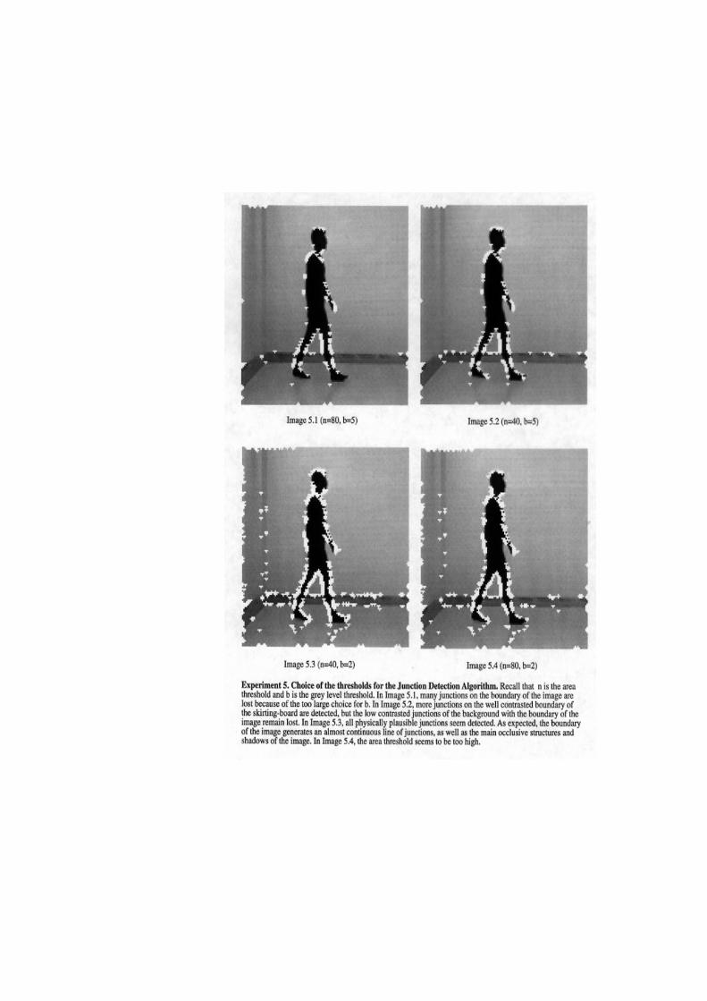
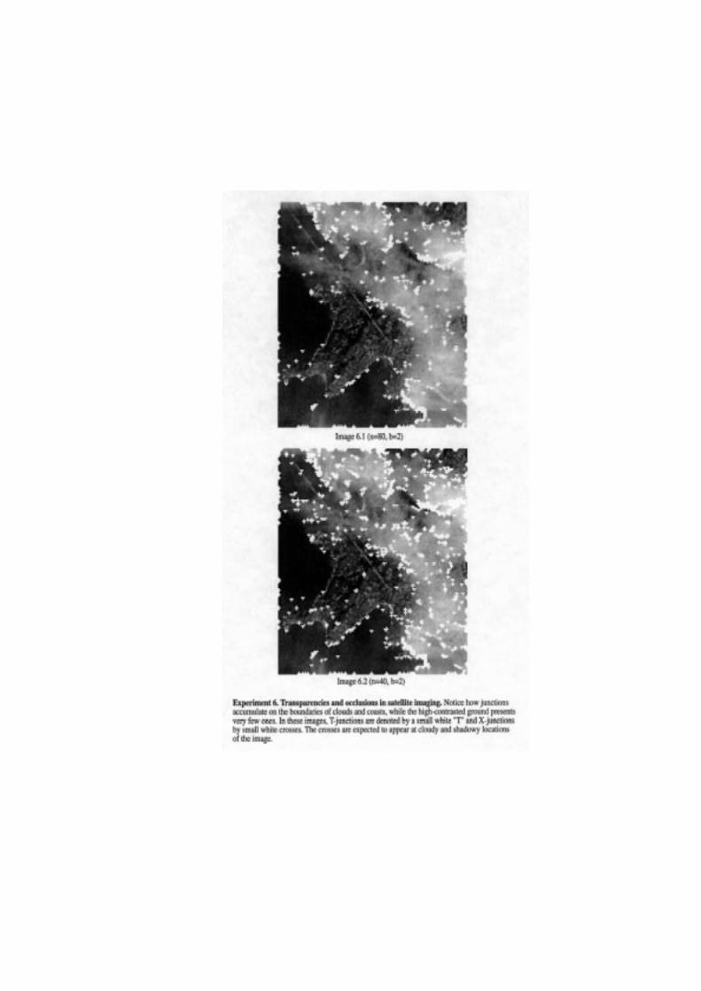
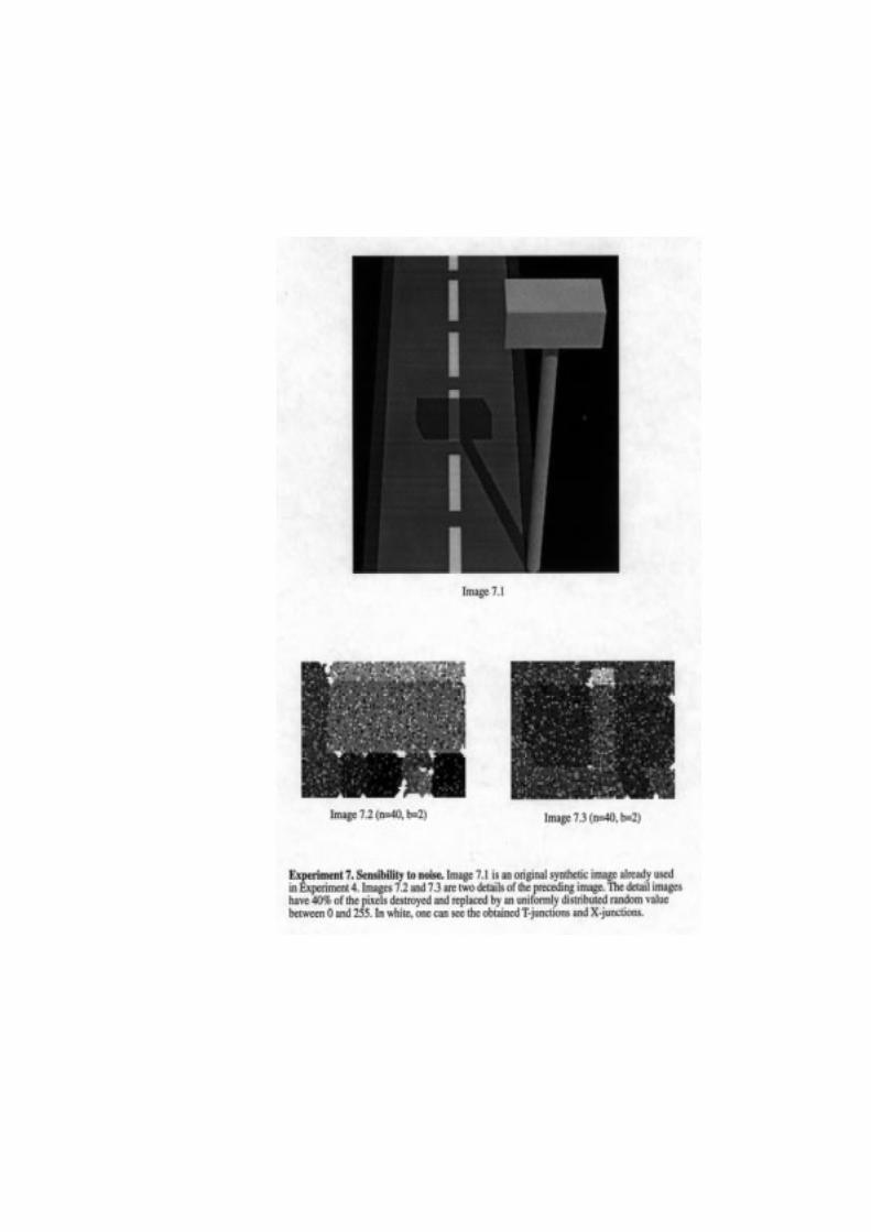
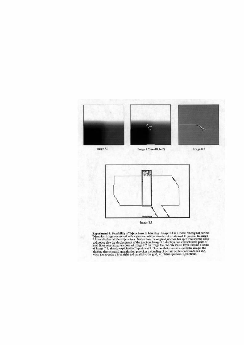
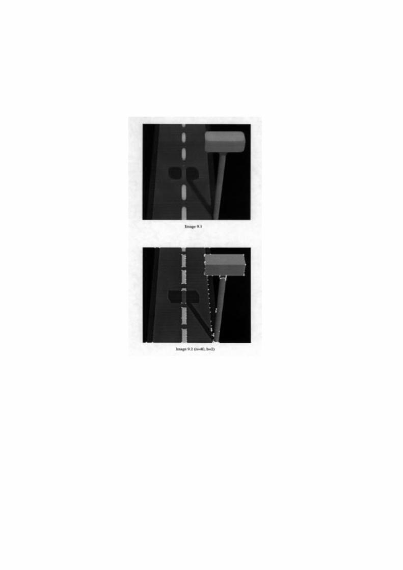
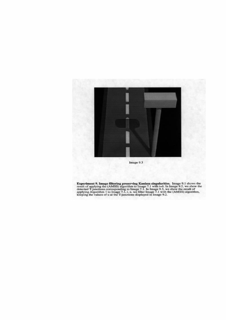
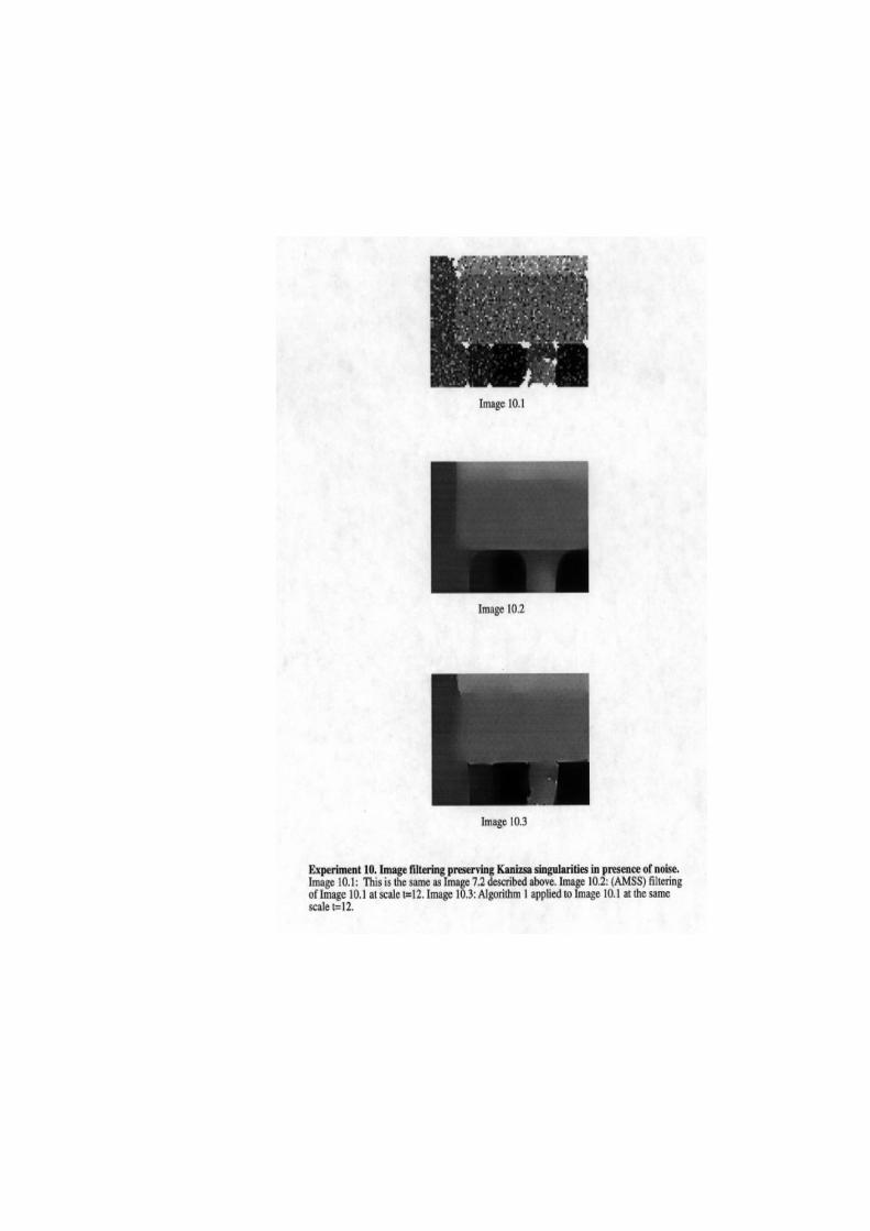
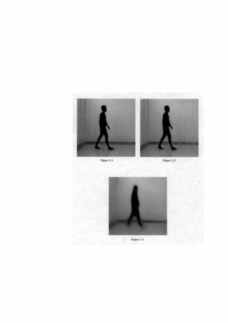
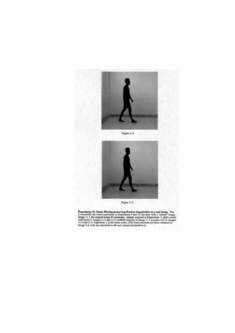
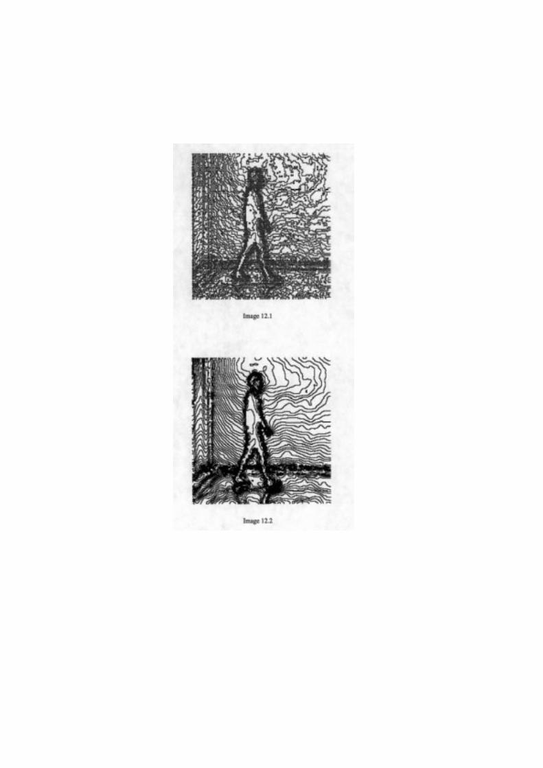
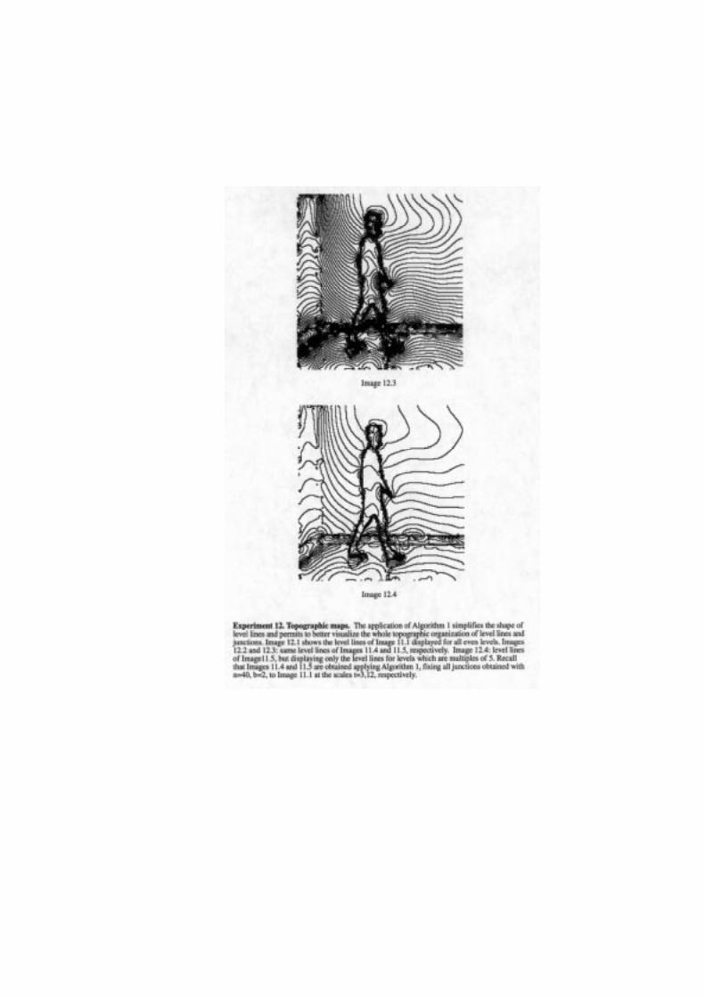
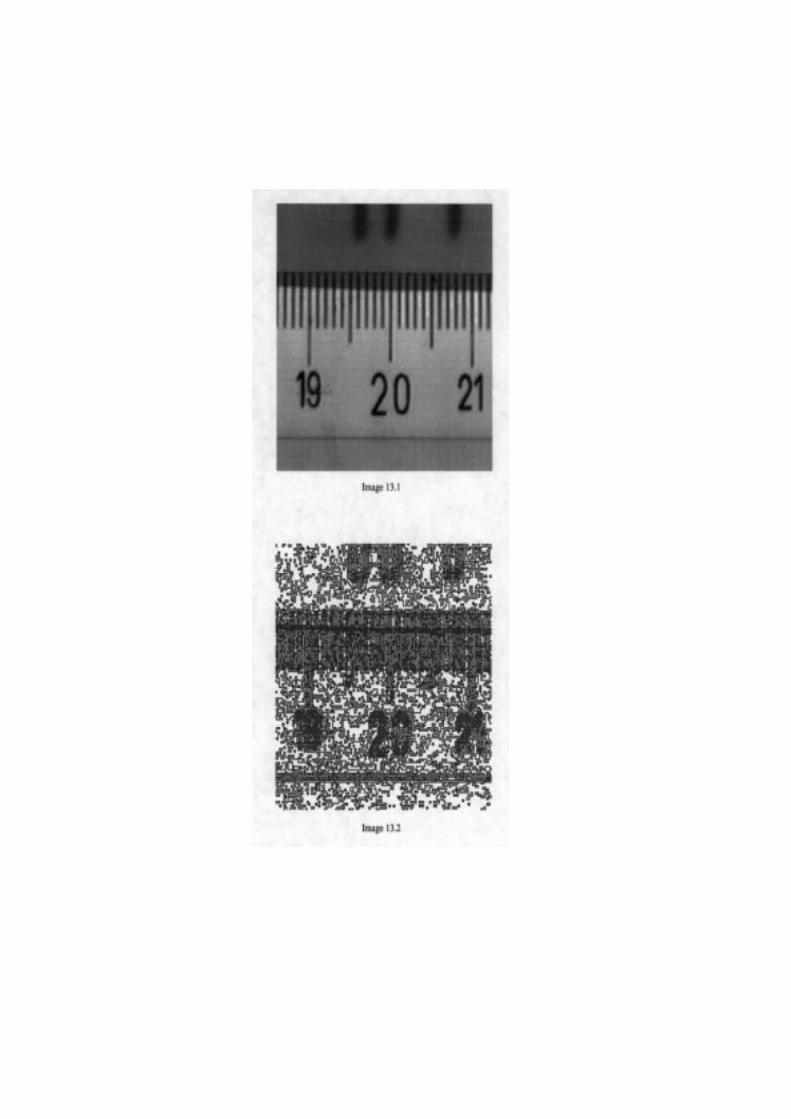
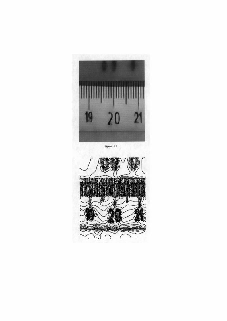
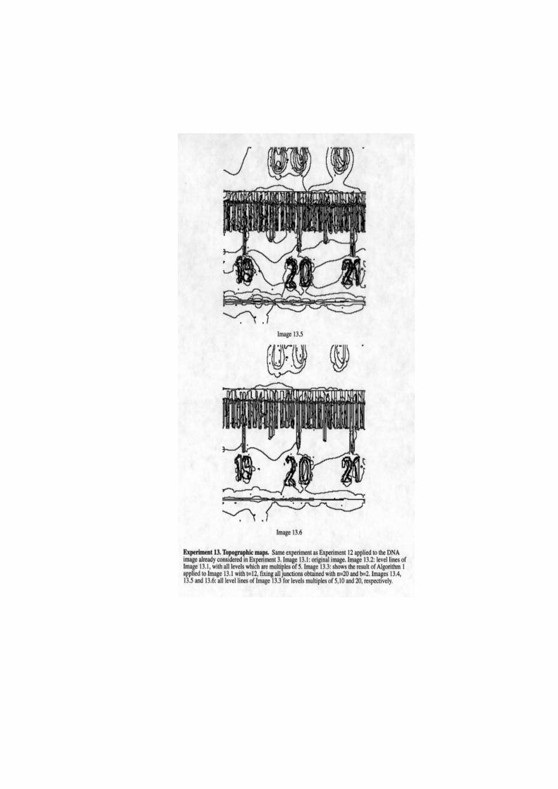
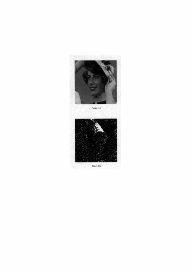
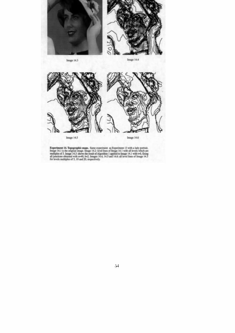
54

7 References

[A] J. Alison Noble. Finding half boundaries and junctions in images. Image and VisionComputing, vol.10, 4, may 1992.

[AGLM1] L. Alvarez, F. Guichard, P.L. Lions and J.M. Morel , Axioms and fundamentalequations of image processing Report 9216, 1992 CEREMADE. Universit�e Paris Dauphine. Arch. for Rat. Mech. 16, IX, 200-257, 1993

[AGLM2] L. Alvarez, F. Guichard, P.L. Lions and J.M. Morel , Axiomatisation et nou-veaux op�erateurs de la morphologie mathematique, C.R. Acad. Sci. Paris, t.315, S�erie I265{268, 1992.

[ALM] L. Alvarez, P.L. Lions and J.M. Morel , Image selective smoothing and edge de-tection by nonlinear di�usion (II), SIAM Journal on numerical analysis 29, 845{866, 1992.

[AM1] L. Alvarez and J.M. Morel. Formalization and Computational Aspects of Im-age Analysis, Acta Numerica, 1994, Cambridge University Press.

[AM] L. Alvarez and Freya Morales. A�ne Morphological Multiscale Analysis of Cor-ners and Multiple Junctions. Ref 9402, August 1994, Dept. Informatica y Systemas,Universidad de Las Palmas de Gran Canaria. To appear in International Journal of Com-puter Vision.

[Ar] R. Arnheim. Art and visual perception : a psychology of the creative eye, 1954.

[Ar] R. Arnheim. Arte e percezione visiva, Feltrinelli, Milano, (tenth edition), 1993.

[BMO] B. Merriman, J. Bence and S.Osher, Motion of multiple junctions : a level setapproach, CAM Report 93-19. Depart. of Mathematics. University of California, LosAngeles CA, June 1993.

[CCCD] V. Caselles, F. Catt�e, T. Coll and F. Dibos. A geometric model for active con-tours in image processing. Numerische Mathematik, 66, 1-31, 1993.

[CGG] Y.G. Chen, Y. Giga and S. Goto. Uniqueness and existence of viscosity solu-tions of generalized mean curvature ow equations. J. Di�. Geometry, 33, 749-786, 1991.

[CIL] M.G. Crandall, H. Ishii and P.L. Lions , User's guide to viscosity solutions of secondorder partial di�erential equation, Bull. Amer. Math. Soc., 27, 1-67, 1992.

[DG] R. Deriche and G. Giraudon. A computational approach for corner and vertexdetection, International Journal of Computer Vision, 10, 2. 101-124, 1993.

[ES] L. C. Evans and J. Spruck. Motion of level sets by mean curvature. J. Di�eren-tial Geom., (33): 635-681, 1991.

55

[F] W. Fuchs. Experimentelle Untersuchungen ueber das simultane Hintereinandersehenauf der selben Sehrichtung, Zeitschrift fuer Psychologie, 91, 154-253, 1923

[GH] M. Gage and R.S. Hamilton , The heat equation shrinking convex plane curves,J. Di�erential Geometry 23, 69{96, 1986.

[GGIS] Y. Giga, S. Goto, H. Ishii and M.M. Sato. Comparison principle and convexitypreserving properties for singular degenerate parabolic equations on unbounded domains.Indiana Univ. Math. J., 40, 443-470, 1991.

[Gr] M. Grayson, The heat equation shrinks embedded plane curves to round points,J. Di�erential Geometry 26, 285{314, 1987.

[Ka1] G. Kanizsa. Organization in Vision, N.Y. Praeger, 1979.

[Ka2] G. Kanizsa. Grammatica del Vedere, Il Mulino, Bologna, 1980.

[Ka3] G. Kanizsa Vedere e pensare, Il Mulino, Bologna, 1991.

[KVD] J.J. Koenderink and A.J. van Doorn , Representation of Local Geometry in theVisual System, Biol. Cyb. 55, 367{375, 1987.

[Koe] J.J. Koenderink. Solid Shape, MIT Press, Cambridge, MA, 1990.

[KTZ] B.B. Kimia, A. Tannenbaum, and S.W. Zucker , On the evolution of curves viaa function of curvature, 1: the classical case, J. of Math. Analysis and Applications 163,No 2, 1992.

[Li] T. Lindeberg. Junction detection with automatic selection of detection scales andlocalization scales, Proc. First Int. Conf. on Image Processing, Austin, Texas, Vol 1,924-928, Nov. 1994

[Ma] D. Marr. Vision N.York, W.H. Freeman and Co, 1982.

[Me] Y. Meyer. Les ondelettes, algorithmes et applications, Armand Colin, Paris, 1992.

[Met] W. Metzger. Gesetze des Sehens, Waldemar Kramer, Frankfurt am Main, 1975.

[MS] J.M. Morel and S. Solimini. Variational methods in image processing, Birkh�auser,1994.

[MSh] D. Mumford and J. Shah, Optimal approximations of piecewise smooth functionsand associated variational problems, Comm. in Pure and Appl. Math., 42, 577-685, 1989

[NMS] M. Nitzberg, D.Mumford and T. Shiota. Filtering, Segmentation and Depth. Lec-

56

ture Notes in Computer Science, 662, Springer-Verlag 1993.

[NM] M. Nitzberg and D. Mumford. "The 2.1 Sketch", in Proceedings of the ThirdInternational Conference on Computer Vision, Osaka 1990.

[OS] S. Osher and J. Sethian, Fronts propagating with curvature dependent speed: al-gorithms based on the Hamilton-Jacobi formulation, J. Comp. Physics 79, 12{49, 1988.

[Ru] L.I. Rudin. Images, numerical analysis of singularities and shock �lters. PhDdissertation, Caltech, Pasadena , California n5250:TR, 1987.

[ST1] G. Sapiro and A. Tannenbaum. On a�ne plane curve evolution. Journal of Func-tional Analysis, 119, 1, 79-120, 1994.

[ST2] G. Sapiro and A. Tannenbaum. A�ne invariant scale space. Int. J. of Com-puter Vision, 11, 24-44, 1993.

[VE] T. Van E�elterre. Calcul Exact du Graphe d'Aspect de Solides de Revolution. Thsede Doctorat, Universit de Rennes I, Janvier 1995.

[We] M. Wertheimer. Untersuchungen zur Lehre der Gestalt, II, Psychologische Forschung,vol. 4, pp.301-350, 1923.

[Wi2] A.P. Witkin. Scale-space �ltering. Proc. of IJCAI, Karlsruhe 1983, 1019-1021.

[Wi] L. Williams. Perceptual organization of occluding contours, Proceedings of the thirdInternational Conference on Computer Vision, Osaka 1990.

57