i

A HYBRID RECONFIGURABLE COMPUTER

INTEGRATED MANUFACTURING CELL FOR MASS

CUSTOMISATION

Submitted by:

Mr N. Hassan - 203510782

BSc Eng, UKZN

School of Mechanical Engineering

Supervisor:

Prof. Glen Bright

May 2011

Submitted in fulfilment of the academic requirements for the degree of Master of Science in Engineering at the School of Mechanical Engineering, University of KwaZulu Natal.

ii

Declarations

Declaration by supervisor:

As the candidate’s Supervisor I agree/do not agree to the submission of this dissertation:

Signed: ..............................

Declaration by Author:

I, Nazmier Hassan, declare that

(i) The research reported in this dissertation/thesis, except where otherwise

indicated, is my original work.

(ii) This dissertation/thesis has not been submitted for any degree or examination at

any other university.

(iii) This dissertation/thesis does not contain other persons’ data, pictures, graphs or

other information, unless specifically acknowledged as being sourced from

other persons.

(iv) This dissertation/thesis does not contain other persons’ writing, unless

specifically acknowledged as being sourced from other researchers. Where

other written sources have been quoted, then:

a) their words have been re-written but the general information attributed to

them has been referenced;

b) where their exact words have been used, their writing has been placed inside

quotation marks, and referenced.

(v) Where I have reproduced a publication of which I am an author, co-author or

editor, I have indicated in detail which part of the publication was actually

written by myself alone and have fully referenced such publications.

(vi) This dissertation/thesis does not contain text, graphics or tables copied and

pasted from the Internet, unless specifically acknowledged, and the source

being detailed in the dissertation/thesis and in the References sections.

Signed: ……………………

iii

Acknowledgements

I thank God Almighty for the guided spiritual support and will-power he has provided me

throughout this research. I owe the greatest gratitude to my parents for their affection. I also

like to thank them for the strength and determination they have embedded in me, in support

of this research.

In admiration to Professor Glen Bright, I thank him for the supervision, motivation and

support throughout this research. He has also granted me valuable experiences in the

duration of this research which will be of tremendous benefit to my future.

I would also like to thank the following people and departments:

The staff at the School of Mechanical Engineering (UKZN) for their outstanding

support.

Mr. Greg Loubser for his tremendous electronic assistance.

Mr. Jared Padayachee, Mr. Anthony Walker, Dr. Riaan Stopforth, Mr. Louwrens

Butler and Mr. Shaniel Davrajh for their guidance.

My colleagues at the Mechatronic and Robotic Research Group for their assistance.

iv

Abstract

Mass producing custom products requires an innovative type of manufacturing environment.

Manufacturing environments at present do not possess the flexibility to generate mass

produced custom products. Manufacturers’ rapid response in producing these custom

products in relation to demand, yields several beneficial results from both a customer and

financial perspective. Current reconfigurable manufacturing environments are yet neither

financially feasible nor viable to implement. To provide a solution to the production of mass

customised products, research can facilitate the development of a distinctive hybrid

manufacturing cell, composed of characteristics inherent in existing manufacturing

paradigms.

Distinctive hybrid manufacturing cell research and development forms an environment

where Computer Integrated Manufacturing (CIM) cells operate in a Reconfigurable

Manufacturing environment. The development of this Hybrid Reconfigurable Computer

Integrated Manufacturing (HRCIM) cell resulted in functionalities that enabled the

production of mass customised products. Manufacturing characteristics of the HRCIM cell

were composed of key Reconfigurable Manufacturing System (RMS) features and CIM

capabilities.

This project required hardware to be used in developing an integrated HRCIM cell.

The cell consisted of storage systems, material handling equipment and processing stations.

Specific material handling equipment was enhanced in its functionality by incorporating

RMS characteristics to its existing structure. The hardware behaviour was coordinated from

software. This facilitated the autonomous HRCIM cell behaviour which was derived from

the mechatronic approach. The software composed of HRCIM events that were defined by

its unique programming language. Highlighted software functionalities included

prioritisation scheduling that resulted from customer order input. Performance data, extracted

from each type of equipment, were used to parameterise a simulated HRCIM cell. During

operation, the cell was frequently introduced to an irregular flow of different product

geometries, which required different processing requirements. This irregularity represented

mass customisation. The simulated HRCIM cell provided detailed manufacturing results.

Significant results consisted of storage times, queueing times and cycle times.

v

List of Acronyms and Abbreviations

AGV Autonomous Guidance Vehicle

AMIA Automated Modular Inspection Apparatus

AMSs Advanced Manufacturing Systems

API Application Programming Interface

ASRS Automated Storage and Retrieval System

CAD Computer-Aided Design

CAM Computer-Aided Manufacturing

CIM Computer Integrated Manufacturing

CNC Computer Numerical Control

DMSs Dedicated Manufacturing Systems

DMLs Dedicated Manufacturing Lines

DOF Degrees of Freedom

FIFO First in first out

FMSs Flexible Manufacturing Systems

GT Group Technology

GUI Graphical User Interface

HRCIM Hybrid Reconfigurable Computer Integrated Manufacturing

I/O Input/Output

JIT Just In Time

Kg Kilograms

MC Mass Customisation

MCP Master Control Program

m metres

mm millimetres

NC Numerical Control

PCB Printed circuit board

RI Robot input

RMSs Reconfigurable Manufacturing Systems

RO Robot output

RPM Revolutions per minute

USART Universal Asynchronous Receiver/Transmitter

WIP Work in process

vi

Table of Contents

Declarations ............................................................................................................................. ii

Acknowledgements ................................................................................................................. iii

Abstract ................................................................................................................................... iv

List of Acronyms and Abbreviations ....................................................................................... v

List of Tables .......................................................................................................................... xi

List of Figures ....................................................................................................................... xiii

Nomenclature ....................................................................................................................... xvii

1. Introduction ......................................................................................................................... 1

1.1 Current Outline of Mass Customisation ......................................................................... 1

1.2 Distinctive Solution to Mass Customisation .................................................................. 1

1.3 Research Objectives ....................................................................................................... 2

1.4 Research Publications .................................................................................................... 2

1.5 Dissertation Structure ..................................................................................................... 3

1.6 Chapter Summary .......................................................................................................... 4

2. Relevant Manufacturing Theory Analysis .......................................................................... 5

2.1 Mass Customisation ....................................................................................................... 5

2.2 Manufacturing Strategies ............................................................................................... 8

2.2.1 Dedicated Manufacturing Systems ......................................................................... 8

2.2.2 Flexible Manufacturing Systems ............................................................................. 8

2.2.3 Reconfigurable Manufacturing Systems ............................................................... 10

2.2.4 Comparison of Manufacturing Systems ................................................................ 12

2.2.5 Computer Integrated Manufacturing ..................................................................... 14

2.3 Relevant Manufacturing Control and Automation Concepts ....................................... 15

2.3.1 Hierarchy of Manufacturing Control and Automation .......................................... 15

2.3.2 Intelligent Agent Based Approach for Manufacturing .......................................... 17

2.4 Chapter Summary ........................................................................................................ 19

vii

3. HRCIM Cell Design Methodology ................................................................................... 20

3.1 The Design Approach .................................................................................................. 20

3.2 Conceptualising the HRCIM Cell ................................................................................ 21

3.2.1 Hardware Architecture .......................................................................................... 22

3.2.2 Software Architecture ........................................................................................... 23

3.2.3 Software/Hardware Coordination ......................................................................... 23

3.3 HRCIM Cell Specifications ......................................................................................... 23

3.4 Chapter Summary ........................................................................................................ 25

4. Manufacturing Cell Design ............................................................................................... 26

4.1 Material Handling Platforms ........................................................................................ 28

4.1.1 Autonomous Guidance Vehicle for Process Integration ....................................... 28

4.1.2 Conveyors ............................................................................................................. 29

4.1.3 Robotic Arm .......................................................................................................... 29

4.2 Buffer Systems ............................................................................................................. 31

4.2.1 Automated Storage and Retrieval System ............................................................. 31

4.2.2 Intermediate Buffer ............................................................................................... 34

4.3 Processing Stations ...................................................................................................... 34

4.3.1 CNC Machine ....................................................................................................... 34

4.3.2 AMIA .................................................................................................................... 35

4.4 Part Library and Flow .................................................................................................. 36

4.4.1 Part Library ........................................................................................................... 36

4.4.2 Part Flow ............................................................................................................... 37

4.5 Chapter Summary ........................................................................................................ 37

5. Mechanical Design ............................................................................................................ 38

5.1 Mechanical Support Structure for the Robot Vision Camera ...................................... 38

5.1.1 Welding Procedure ................................................................................................ 39

5.1.2 Cantilever Beam Deflection .................................................................................. 41

5.2 Reconfigurable Robotic Arm End Effector .................................................................. 42

viii

5.2.1 End Effector Interfaces ......................................................................................... 42

5.2.1.1 Interface Requirements .................................................................................. 46

5.2.2 End Effector Actuation ......................................................................................... 48

5.3 Tool Holding Table ...................................................................................................... 53

5.4 ASRS Motor/Encoder Interface ................................................................................... 54

5.5 Chapter Summary ........................................................................................................ 54

6. Electronic Design .............................................................................................................. 55

6.1 Device Level Electronic Applications ......................................................................... 55

6.1.1 Light Dependent Resistor ...................................................................................... 55

6.1.2 Encoders ................................................................................................................ 57

6.1.3 Limit Switches ...................................................................................................... 58

6.1.4 Relays to Control ASRS Crane Movement ........................................................... 59

6.1.5 Relays to Control Circular Conveyor Movement ................................................. 60

6.1.6 A Step-up Voltage Logic Circuit .......................................................................... 60

6.2 Intermediate Manufacturing Cell Controllers .............................................................. 62

6.2.1 Microcontrollers .................................................................................................... 62

6.2.1.1 Universal Asynchronous Receiver/Transmitter ............................................. 64

6.2.2 Data Acquisition Control ...................................................................................... 64

6.2.3 Robot I/O ............................................................................................................... 66

6.3 Master Manufacturing Cell Controller ......................................................................... 67

6.4 Controller Integration ................................................................................................... 69

6.5 Chapter Summary ........................................................................................................ 71

7. Software Design ................................................................................................................ 72

7.1 Featured Visual Basic Applications ............................................................................. 72

7.2 C Language Applications ............................................................................................. 75

7.3 Robotic Arm Teaching ................................................................................................. 76

7.3.1 iRvision Software .................................................................................................. 77

7.4 Chapter Summary ........................................................................................................ 79

ix

8. Testing and Results ........................................................................................................... 80

8.1 Algorithm Based Priority Scheduling .......................................................................... 80

8.2 Equipment Testing ....................................................................................................... 82

8.2.1 Part Dependent Operations ................................................................................... 82

8.2.1.1 ASRS Testing ................................................................................................. 82

8.2.1.2 Robotic Arm Testing ...................................................................................... 83

8.2.2 Part Independent Operations ................................................................................. 83

8.3 Simulating the HRCIM Cell......................................................................................... 84

8.3.1 Hardware Analysis ................................................................................................ 87

8.3.1.1 ASRS Analysis ............................................................................................... 87

8.3.1.2 AGV Analysis ................................................................................................ 89

8.3.1.3 Conveyor Analysis for Processing Cell 1 ...................................................... 90

8.3.1.4 CNC Machine Analysis.................................................................................. 92

8.3.1.5 Robot 1 and 2 Analysis .................................................................................. 95

8.3.1.6 Conveyor 2 Analysis in Processing Cell 2 ..................................................... 96

8.3.1.7 AMIA Analysis .............................................................................................. 97

8.3.2 Part Analysis ......................................................................................................... 98 

8.4 Chapter Summary ...................................................................................................... 106 

9.  Discussion ....................................................................................................................... 107 

9.1 Performance Measures Prior to HRCIM Cell Simulation .......................................... 107 

9.1.1 Mechanical Constraints ....................................................................................... 107 

9.1.2 Electronic Constraints ......................................................................................... 107 

9.1.3 Software Constraints ........................................................................................... 108 

9.2 Measured Values to Parameterise the HRCIM Cell Simulation ................................ 108 

9.3 Simulated Results ....................................................................................................... 108 

9.4 Reviewed HRCIM Cell Objectives ............................................................................ 109 

9.5 HRCIM in Comparison to RMS and FMS ................................................................. 109 

9.6 Observed HRCIM Cell Restrictions and Complications ............................................ 111 

9.6.1 Accuracy and Repeatability ................................................................................ 111 

9.6.2 Robotic Vision Calibration ................................................................................. 111 

x

9.6.3 Limitations within RMS Technology .................................................................. 111 

9.6.4 Research Assumptions ........................................................................................ 112 

9.6.5 Restrictions within the HRCIM Cell Simulation ................................................ 112 

9.7 Chapter Summary ...................................................................................................... 112 

10. Conclusion ..................................................................................................................... 113 

11. References ...................................................................................................................... 116 

Appendices ........................................................................................................................... 121 

Appendix A ...................................................................................................................... 122 

Appendix B ...................................................................................................................... 126 

Appendix C ...................................................................................................................... 131 

Appendix D ...................................................................................................................... 142 

Appendix E ...................................................................................................................... 145 

Please find relevant engineering drawings and the manufacturing simulation copied to the

CD provided.

xi

List of Tables

Table 2-1: Comparing DMS, RMS and FMS characteristics ................................................. 13 

Table 3-1: HRCIM cell specifications ................................................................................... 24 

Table 4-1: Equipment labelling in Figure 4-1 ........................................................................ 27 

Table 5-1: Required weld height for specified weld .............................................................. 40 

Table 5-2: Technical specifications for the tool changing unit .............................................. 43 

Table 5-3: Technical specifications for the grippers .............................................................. 44 

Table 5-4: Calculated results for interface failure .................................................................. 47 

Table 5-5: Calculated results for 2-finger gripper interfaces ................................................. 47 

Table 5-6: Calculated results for 3-finger gripper interfaces ................................................. 47 

Table 5-7: Joint separation force in comparison to the external weight subjected ................ 48 

Table 6-1: ASRS crane distance per encoder revolution ....................................................... 58 

Table 6-2: µDAQLite technical specifications ...................................................................... 65 

Table 6-3: Robot I/O pin description and functionality ......................................................... 67 

Table 6-4: µDAQ technical specifications ............................................................................. 69 

Table 6-5: Coordinated and synchronised controller behaviour at logic high ....................... 70 

Table 6-6: Device feedback to microcontroller pins .............................................................. 71 

Table 6-7: μDAQLite pin and vision processing functionalities ........................................... 71 

Table 7-1: Examples of applying a logic high for selected µDAQ port pins ......................... 73 

Table 7-2: Examples of applying a logic high for selected µDAQLite channels .................. 73 

Table 8-1: Customer order input values and processing times .............................................. 81 

Table 8-2: ASRS retrieval time per part type ......................................................................... 82 

Table 8-3: Robot 1 material handling time per part type ....................................................... 83 

Table 8-4: Robot 2 material handling time per part type ....................................................... 83 

Table 8-5: Conveyor speeds ................................................................................................... 83 

Table 8-6: Simio object definition and hardware represented ............................................... 85 

APPENDIX C Table C-1: Specifications for Interface C ............................................................................ 131 

Table C-2: Interface a specifications for the 2-Finger parallel gripper ................................ 133 

Table C-3: Interface b specifications for the 2-Finger parallel gripper ................................ 134 

Table C-4: Interface a + b specifications for the 2-Finger parallel gripper .......................... 135 

Table C-5: Interface a specifications for the 3-Finger centric gripper ................................. 137 

Table C-6: Interface b specifications for the 3-Finger centric gripper ................................. 138 

xii

Table C-7: Interface a + b specifications for the 3-Finger centric gripper ........................... 140

APPENDIX D

Table D-1: ASRS part retrieval time from the reference point ............................................ 142 

Table D-2: ASRS part retrieval time from the unloading point ........................................... 143 

Table D-3: Robot 1 material handling time per part type .................................................... 143 

Table D-4: Robot 1 material handling time per part type subsequent to gripper

reconfiguration ..................................................................................................................... 143 

Table D-5: Robot 2 material handling time per part type .................................................... 143 

Table D-6: CNC machine changeover matrix ...................................................................... 144 

Table D-7: Part travel time for conveyor 1 & 2 ................................................................... 144 

xiii

List of Figures

Figure 2-1: Weighing MC to product variety .......................................................................... 6 

Figure 2-2: Manufacturing strategies in contrast ..................................................................... 6 

Figure 2-3: MC with respect to product variety (customisation) and time-cost factors ........... 7 

Figure 2-4: Typical FMS layout ............................................................................................... 9 

Figure 2-5: Reconfigurable CNC drilling machine with varying DOF ................................. 11 

Figure 2-6: CNC drilling machine modules ........................................................................... 11 

Figure 2-7: Manufacturing strategies in relation to capacity and product variety ................. 13 

Figure 2-8: Manufacturing strategies in relation to capacity and system cost ....................... 14 

Figure 2-9: Corresponding CIM functionalities ..................................................................... 15 

Figure 2-10: Hierarchy of manufacturing control and automation ........................................ 16 

Figure 2-11: Diagram describing an agent ............................................................................. 18 

Figure 3-1: Diagram illustrating the mechatronic approach .................................................. 20 

Figure 3-2: Vena diagram for the HRCIM cell implementation ............................................ 21 

Figure 4-1: HRCIM cell layout .............................................................................................. 26 

Figure 4-2: Physical cell setup - view 1 ................................................................................. 27 

Figure 4-3: Physical cell setup - view 2 ................................................................................. 28 

Figure 4-4: AGV for HRCIM cell process integration .......................................................... 29 

Figure 4-5: Fanuc robotic arm ............................................................................................... 30 

Figure 4-6: Robot restrictions in space .................................................................................. 30 

Figure 4-7: ASRS ................................................................................................................... 32 

Figure 4-8: ASRS coordinates ............................................................................................... 33 

Figure 4-9: ASRS storage points ........................................................................................... 33 

Figure 4-10: Johnford VMC-850 CNC milling machine ....................................................... 34 

Figure 4-11: AMIA ................................................................................................................ 35 

Figure 4-12: Library of parts .................................................................................................. 36 

Figure 4-13: Substitution for part type ................................................................................... 36 

Figure 4-14: Part flow ............................................................................................................ 37 

Figure 5-1: Vision camera support platform. ......................................................................... 38 

Figure 5-2: Camera support structure .................................................................................... 40 

Figure 5-3: Deflection υ of vision camera ............................................................................. 41 

Figure 5-4: Interface c for quick-change head attachment ..................................................... 44 

Figure 5-5: 2-Finger gripper module...................................................................................... 45 

Figure 5-6: 3-Finger gripper module...................................................................................... 45 

xiv

Figure 5-7: Solenoid valve setup on the robotic arm ............................................................. 49 

Figure 5-8: Pneumatic flow diagram for gripper reconfiguration and finger actuation ......... 50 

Figure 5-9: 5/2 way solenoid valve logic diagram ................................................................. 51 

Figure 5-10: 5/3 way solenoid valve logic diagram ............................................................... 52 

Figure 5-11: Tool (gripper) holding table .............................................................................. 53 

Figure 5-12: Supports for respective grippers ........................................................................ 53 

Figure 5-13: Encoder/ASRS pulley coupling ........................................................................ 54 

Figure 6-1: LDR setup ........................................................................................................... 55 

Figure 6-2: LDR response chart ............................................................................................. 56 

Figure 6-3: LDR circuit diagram ........................................................................................... 56 

Figure 6-4: Encoder with wiring colour code table ............................................................... 57 

Figure 6-5: Limit switch ........................................................................................................ 58 

Figure 6-6: 15 Amp relay circuit ............................................................................................ 59 

Figure 6-7: 30 Amp relay circuit ............................................................................................ 60 

Figure 6-8: 5/24 volt step up logic circuit .............................................................................. 61 

Figure 6-9: Pin layout for the ATmega32L microcontroller .................................................. 62 

Figure 6-10: PCB for Atmega32L microcontroller ................................................................ 63 

Figure 6-11: USB-serial interface connector ......................................................................... 64 

Figure 6-12: Eagle µDAQLite for data acquisition ................................................................ 65 

Figure 6-13: Robotic arm I/O pins ......................................................................................... 66 

Figure 6-14: Pin layout for end effector interface (RI/RO) ................................................... 67 

Figure 6-15: Front and back view of the Eagle µDAQ 120A ................................................ 68 

Figure 6-16: Pin configuration for the µDAQ Digital I/O male connector ........................... 68 

Figure 6-17: Controller integration ........................................................................................ 69 

Figure 7-1: API read and write functions ............................................................................... 73 

Figure 7-2: MCP GUI developed with VB6 .......................................................................... 74 

Figure 7-3: MCP with customer input values ........................................................................ 74 

Figure 7-4: Code snippet for position control ........................................................................ 75 

Figure 7-5: Logic diagram for ASRS position control ........................................................... 76 

Figure 7-6: Teach pendant ..................................................................................................... 77 

Figure 7-7: iRvision accessed from the Microsoft Internet Explorer framework .................. 78 

Figure 7-8: iRvision software interface .................................................................................. 78 

Figure 8-1: EgdeCam part simulator ...................................................................................... 81 

Figure 8-2: Priority values for each customer order .............................................................. 81 

Figure 8-3: Simio main frame ................................................................................................ 84 

xv

Figure 8-4: Simio 2D overview of the HRCIM cell............................................................... 85 

Figure 8-5: Simio 3D overview of the HRCIM cell............................................................... 86 

Figure 8-6: ASRS retrieval time per part ............................................................................... 87 

Figure 8-7: ASRS retrieval time for first three parts .............................................................. 88 

Figure 8-8: Pie chart indicating ASRS resource state ............................................................ 88 

Figure 8-9: Simio report for the ASRS .................................................................................. 89 

Figure 8-10: Simio report for the AGV .................................................................................. 90 

Figure 8-11: Part buffering time at the vision processing platform of conveyor 1 ................ 91 

Figure 8-12: Reduced time frame showing part buffering time at the vision processing

platform .................................................................................................................................. 91 

Figure 8-13: Simio report for Conveyor 1 ............................................................................. 92 

Figure 8-14: Graph illustrating part entry and exit time at the CNC machine ....................... 93 

Figure 8-15: Graph with reduced time frame indicating CNC machine part entry and exit .. 93 

Figure 8-16: Simio report for the CNC workstation .............................................................. 94 

Figure 8-17: Simio report for Robot 1 and Robot 2 ............................................................... 96 

Figure 8-18: Conveyor analysis before the AMIA ................................................................ 97 

Figure 8-19: Conveyor analysis after the AMIA ................................................................... 97 

Figure 8-20: Graph mapping the AMIA vision processing time intervals per part ............... 97 

Figure 8-21: Simio generated results for the AMIA .............................................................. 98 

Figure 8-22: Graph indicating the initial retrieval time for all part types .............................. 99 

Figure 8-23: Graph indicating the initial retrieval time for part type A ................................. 99 

Figure 8-24: Graph indicating the initial retrieval time for part type D ............................... 100 

Figure 8-25: Graph indicating the initial retrieval time for part type C ............................... 100 

Figure 8-26: Graph indicating the initial retrieval time for part type B ............................... 101 

Figure 8-27: Simio report for the Source ............................................................................. 101 

Figure 8-28: Graph indicating the time for which parts exit the HRCIM cell ..................... 102 

Figure 8-29: Time for which part type A exits the manufacturing cell ................................ 102 

Figure 8-30: Time for which part type D exits the manufacturing cell ................................ 103 

Figure 8-31: Time for which part type C exits the manufacturing cell ................................ 103 

Figure 8-32: Time for which part type B exits the manufacturing cell ................................ 104 

Figure 8-33: Simio report for the Sink ................................................................................. 104 

Figure 8-34: Time for which the first part of customer order one is initiated for retrieval .. 105 

Figure 8-35: Time for which the first part of customer one exits the manufacturing cell ... 105 

Figure 8-36: Simio report for part types produced ............................................................... 106 

xvi

APPENDIX A Figure A-1: Camera support ................................................................................................ 122 

Figure A-2: Moment diagram with beam cross section ....................................................... 122 

Figure A-3: Moment diagram for vertical tubular bar and cross sectional drawing ............ 124 

Figure A-4: Retractable height adjustment .......................................................................... 125

APPENDIX B

Figure B-1: Beam deflection diagram .................................................................................. 126 

Figure B-2: Top beam deflection diagram ........................................................................... 127 

Figure B-3: Vertical bar deflection diagram ........................................................................ 129

APPENDIX C

Figure C-1: Interface C ........................................................................................................ 131 

Figure C-2: Interface a for the 2-Finger parallel gripper module ........................................ 132 

Figure C-3: Interface b for the 2-Finger parallel gripper module ........................................ 134 

Figure C-4: Interface a for the 3-Finger centric gripper module .......................................... 137 

Figure C-5: Interface b for the 3-Finger centric gripper module ......................................... 138 

xvii

Nomenclature

A Area of a weld, cross sectional area of a bolt

Ac Clamped area

At Tensile stress area of a bolt

b Base length of weld, beam cross section dimension (base)

C1 Constant

C2 Constant

Cpriority Coefficient of priority

d Height of weld, bolt diameter

E Modulus of elasticity

Eb Modulus of elasticity for a bolt

Ec Modulus of elasticity for interface material

F Bolt tensile load

Fd Direct force

Fe Joint separating force

Fi Initial tensile force

Fs Maximum shear force

g Clamped length

h Weld height, beam cross section dimension (height)

I Moment of inertia

Iu Unit polar of inertia

Kb Bolt stiffness

Kc Interface stiffness

Ki Constant

M Moment

Mo Moment

P Force

Pi Number of parts per order

Pt Part type

PTo Time to produce an order

PTp CNC processing time per part

Sp Proof strength

SSY Shear yield strength

T Shear stress, tightening torque

xviii

Td Time an order is due

Tf Time till due date

Ti Time an order is initiated

Tmax Maximum shear stress

t Nut thickness

x Distance on x-axis

xl x axis linear distance per encoder revolution

y Centre of weld

yl y axis linear distance per encoder revolution

zl z axis linear distance per encoder revolution

Ø Beam slope

σbending Bending stress

σdirect Direct stress

σresultant Resultant stress

υ Beam deflection

1

1. Introduction

1.1 Current Outline of Mass Customisation

Present-day manufacturing industries are incapable of feasibly meeting the flexibility

required to produce mass customised parts or products. Current Advanced Manufacturing

Systems (AMSs) or conventional manufacturing strategies that include Dedicated

Manufacturing Systems (DMSs), Reconfigurable Manufacturing Systems (RMSs), Flexible

Manufacturing Systems (FMSs) and Computer Integrated Manufacturing (CIM) are still

inefficient, incapable or too costly to meet this flexibility [1]. These strategies are ineffectual

of providing modern manufacturing industries with the qualities to respond to current

competitive, stochastic and diverse market behaviour for mass customised parts. This

unstable market behaviour result significantly from individual customer needs for

customised, cost effective, and quality products in combination with short delivery times.

Converging manufacturing towards customer satisfaction generates several beneficial results,

predominantly in gaining market share.

1.2 Distinctive Solution to Mass Customisation

To initiate a directed approach in producing mass customised parts, study of different

manufacturing strategies that included DMSs, RMSs, FMSs and CIM were investigated. To

validate this approach, research relating to mass customisation (MC) was also imperative.

Based on these existing manufacturing concepts, a solution whereby the evolution of a

distinctive hybrid manufacturing cell was initiated to accommodate MC. Its functionality

was specifically in combination of certain RMS and CIM strategies to form a Hybrid

Reconfigurable Computer Integrated Manufacturing (HRCIM) cell.

The HRCIM cell was introduced to key manufacturing applications. These included

the ability to respond to reconfiguration of the cell architecture that arouse from a

dynamically changing scheduling environment. Reconfiguration of the cell architecture

provided seamless manufacturing operations that accommodated changeover between

different part types. Related functionalities incorporated prioritising scheduling and

reconfigurable material handling capabilities for customised parts. Software and hardware

2

integration generated a functional HRCIM cell. At a sophisticated level, basic intelligent

agent approaches were used to develop some software and hardware functionalities.

The HRCIM cell architecture included an Automatic Storage and Retrieval System

(ASRS), Automated Guided Vehicle (AGV), conveyor system, robotic arm with integrated

vision and reconfigurable end effector capabilities, Computer Numerical Control (CNC)

milling machine and an Automated Modular Inspection Apparatus (AMIA).

Software simulation was used to imitate the HRCIM cell environment. The simulation

provided an analysis for a mass customisation-based problem. Some of the analysed

parameters that were essential to this frequently changing manufacturing environment

include cell changeover, manufacturing flexibility, lead time, buffer status, machine capacity

and product cycle time. Moreover, customer satisfaction formed a vital pre-requisite when

considering these manufacturing parameters. The result highlighted the characteristics of the

HRCIM cell, and provides a platform for future research and development in this field.

1.3 Research Objectives

The project objectives were:

To research a solution space for the manufacture of mass customised parts through

the implementation of a HRCIM cell.

To research the incorporation of part variety in material handling systems.

To research and develop a manufacturing cell with sufficient flexibility and

reconfigurability for facilitating the mass production of customised parts.

To provide a HRCIM cell, as required by a manufacturing environment.

To verify project specifications.

1.4 Research Publications

N. Hassan, G. Bright; Optimum Mass Customised Part Production via

Reconfigurable Computer Integrated Manufacturing Cells; 25th ISPE International

Conference on CAD/CAM, Robotics and Factories of the Future; 14-16 July 2010;

Pretoria; South Africa: Section on Advanced Manufacturing.

3

A.J. Walker, L.J. Butler, N. Hassan, G. Bright; Reconfigurable Materials Handling

Control Architecture for Mass Customization Manufacturing; International

Conference on Competitive Manufacturing (COMA ’10); 3-5 February 2010;

Stellenbosch, South Africa; Pages 277-284.

1.5 Dissertation Structure

Chapter 1: Provides a concise justification, methodology and objectives of this research.

Research publications relevant to the research were also listed.

Chapter 2: The study of the existing manufacturing strategies relevant to this research is

interpreted. An approach towards MC and basic understanding of implementing intelligent

agent based platforms is also illustrated.

Chapter 3: Introduces the concept for HRCIM cell development. It also illustrates

disintegration of the HRCIM cell which provides further hardware and software conceptual

guidelines.

Chapter 4: Provides a detailed layout of the HRCIM cell. An illustration and detailed

functionality of the diverse equipment used to construct the HRCIM cell is provided. Entities

based at a MC approach are also demonstrated.

Chapter 5: Illustrates the design, utilisation of mechanical modules and structures for added

HRCIM cell capabilities.

Chapter 6: Illustrates the design and utilisation of electronic modules embedded into the

HRCIM cell for synchronised and refined functionality.

Chapter 7: Provides a disintegration of software developed from a user interface to an

automated level of program execution. It also provides detail relating master to primary

HRCIM cell control activities.

Chapter 8: Details the testing and results of HRCIM cell equipment. Based on these findings,

simulation of a fully integrated HRCIM cell was analysed. A comprehensive feedback of

computed HRCIM cell results is provided.

4

Chapter 9: Provides an interpretation of the HRCIM cell efficiency and capabilities. A

discussion of the HRCIM cell in contrast to existing manufacturing strategies is also

presented.

Chapter 10: Illustrates a recapitulation of the research objectives with respect to HRCIM cell

efficiency and capabilities. It also proposes the limitations and adverse findings that entail

future research.

1.6 Chapter Summary

This opening chapter provided the reader with insight to the research problem. A brief

solution and systematic approach was introduced. Publications relating to this research topic

are listed and an overview of dissertation content is also provided.

5

2. Relevant Manufacturing Theory Analysis

The concept towards developing a HRCIM cell for producing mass customised parts

involved the review of various market and manufacturing related disciplinaries. It focused on

market behaviour from a MC perspective and analysed how it provided a drive for

manufacturing. Conceptualising a reconfigurable CIM cell required the review of different

manufacturing strategies. This included theoretical manufacturing approaches, from

traditional DMS to more recent CIM, FMS and RMS manufacturing strategies. The

following literature survey is structured from a market to a manufacturing based analysis.

This highlighted the significant advantages and disadvantages of each manufacturing

strategy in producing mass customised parts.

2.1 Mass Customisation

Today, there is an abundance of existing products. Customer demands are more diversified

and peoples’ individual thoughts desire something unique [2]. It generates an unsolved space

for manufacturers to confront, particularly in providing mass customised parts. This modern

approach of producing customised parts has constrained manufactures to retain high

production efficiency, good customer gratification, and short delivery and lead times [3].

MC as stated by Tseng et al, can be defined as, "the technologies and systems to

deliver goods and services that meet individual customer needs with near mass production

efficiency" [4]. MC encompasses the idea, “build to order”. This “build to order” concept

limits companies to forecast demands until having attained customer orders [5].

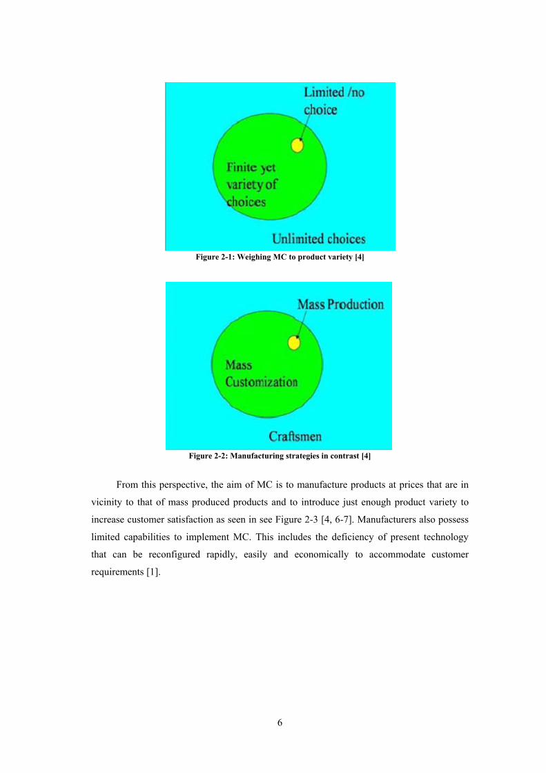
In the form of a vena diagram, Figure 2-1 [4] illustrates the comparison of product

variety in relation to the corresponding manufacturing strategies in Figure 2-2 [4]. As

illustrated in Figure 2-2, MC is a concept that is intermediate with respect to mass

production and craftsmanship. Craftsmanship can be defined as a process where products are

manufactured subsequent to receiving an order. Products are also manufactured according to

customer specification. This strategy involves higher cost and lead times for products. Mass

production in contrast produces low cost and fast delivery of products [4].

6

Figure 2-1: Weighing MC to product variety [4]

From this perspective, the aim of MC is to manufacture products at prices that are in

vicinity to that of mass produced products and to introduce just enough product variety to

increase customer satisfaction as seen in see Figure 2-3 [4, 6-7]. Manufacturers also possess

limited capabilities to implement MC. This includes the deficiency of present technology

that can be reconfigured rapidly, easily and economically to accommodate customer

requirements [1].

Figure 2-2: Manufacturing strategies in contrast [4]

7

Some of the benefits of practising MC include the following [5, 7]:

It meets customer requirements, which in addition moulds a customer relationship,

and increases customer contentment and devotion.

It maximises market share that is merited from increased customer satisfaction and

growth.

It reduces inventory levels. Moreover, MC utilises Just In Time (JIT) production

which reduces material waste and cost. JIT refers to the introduction of material into

the production line or workstation just before it is processed [8].

It provides quick response from receiving to delivering orders. Organisation

configuration and flexible manufacturing strategies enable manufacturers to rapidly

alter their environment to accommodate different product demand patterns in

facilitating MC.

It creates continual opportunities for innovation.

Figure 2-3: MC with respect to product variety (customisation) and time-cost factors [7]

8

2.2 Manufacturing Strategies

2.2.1 Dedicated Manufacturing Systems

DMSs are cost effective, due to fixed automated production lines [9]. They produce parts of

good quality, at high volumes and low cost [10]. Each Dedicated Manufacturing Line (DML)

has the functionality to produce a single part at high production rates. The cost per part is

comparatively low which arise from high product demand [11].

The adverse effects of utilising DMSs include the lack of scalability. This inflexible

condition of DMS, result from the fixed output capacity and cycle times. From a market

perspective, DMSs lacks the flexibility required to provide a competent solution in today’s

market conditions [10].

2.2.2 Flexible Manufacturing Systems

A Flexible Manufacturing System (FMS) can be described as a highly automated machine

cell that is based on CIM technology [12]. It can be further identified as a Group Technology

(GT) based manufacturing system [13]. The application of GT refers to the grouping together

of similar parts that assist in simplifying the design and manufacturing of parts. Similar parts

are categorised into part families, where each part family contains similar design or

manufacturing procedures [8].

A typical FMS layout is composed of a group of processing workstations such as CNC

machine tools, load and unload stations, and inspection stations, as shown in

Figure 2-4 [12]. These are integrated with a storage and automated material handling system

(ASRS), and managed via a distributed computer system [12-13]. A FMS possesses the

capabilities of simultaneously processing a variety of different part styles. In response to

varying demand patterns, a FMS is also able to adjust to changing production quantities and

variations in part styles [8].

Limitations to the manufacture of a range of products or parts exist in an FMS

environment as no manufacturing system is completely flexible. Products or parts are

bounded within a specific range of styles, sizes and processes. In relation to part family,

FMS has the capability of accommodating a single to a limited range of part families.

9

Moreover, to be qualified as an FMS, the system should adapt to a non batch approach. It

must also be able to adjust to scheduling changes in response to production quantity and part

mix [8].

To be flexible, a manufacturing system should meet several capabilities which are

listed as follows [8]:

It must possess the capability to recognise and differentiate between part or product

styles processed by the system following its arrival.

It should possess rapid operational instruction changeover.

It must provide rapid physical setup changeover.

Some of the beneficial results of utilising an FMS approach include [13]:

Improved quality of products.

It reduces lead time (time from initiation to completion of a job).

It reduces inventory levels.

Provides enhanced management control of the complete manufacturing process.

Reduced equipment cost due to flexible capabilities of an FMS.

It requires less factory space.

Despite the many benefits of FMS, it does possess some negative outlines. These

include the complexity of the system, were the built-in functionalities are too excessive and

Figure 2-4: Typical FMS layout [12]

10

in most situations not all of these functionalities are needed. From a financial perspective,

this excessive and unused functionalities yield very high capital cost for FMS equipment. In

relation to the flexibility, FMSs cannot be subjected to change with respect to the fixed,

obsolete software and hardware. This limits a FMS from add-ons, customisation and

upgrading. Additionally, FMSs is designed for low to medium volume productivity and is

therefore not appropriate for great market fluctuations [10].

2.2.3 Reconfigurable Manufacturing Systems

RMS as defined by Koren and Ulsoy, is a system designed for rapid adjustment of

production capacity and functionality, in response to new circumstances, by rearrangement

or change of its components [14].

RMS is a combination of selected FMS and DML characteristics [15]. Previous

research on RMS included machine-level and system-level design issues. Machine-level

design includes modular machine controls. System-level design is initiated from similar

geometric features of a part family. From a system-level, the objective is to form a cost-

effective manufacturing system with an optimal system configuration. In relation to these

objectives, the goal is to facilitate the manufacture of part mix and volume [16].

Essentially, a RMS is defined by its flexibility in producing part variety and its ability

to reconfigure the manufacturing system. Products manufactured in a RMS environment are

grouped into families. Individual product families require a different system configuration

for manufacture. A RMS is designed with the use of hardware and software modules that can

be reconfigured quickly and efficiently [17-18]. Its design enables it to rapidly produce

dissimilar product families without relinquishing quality in the shortest time and at the

lowest cost [19]. The design functionalities of a RMS include removing, adding, or

modifying of certain software, controls, process capabilities or machine structure. These

functionalities allow the system to adhere to production capacities in reply to technological

advancements and fluctuating market demands. From a technological perspective, the open-

ended architecture of a RMS also facilitates upgrading, reconfiguring and system

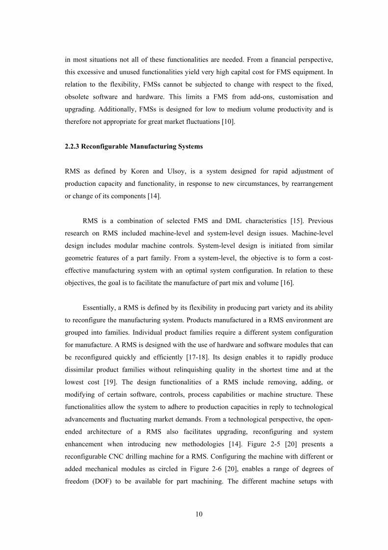
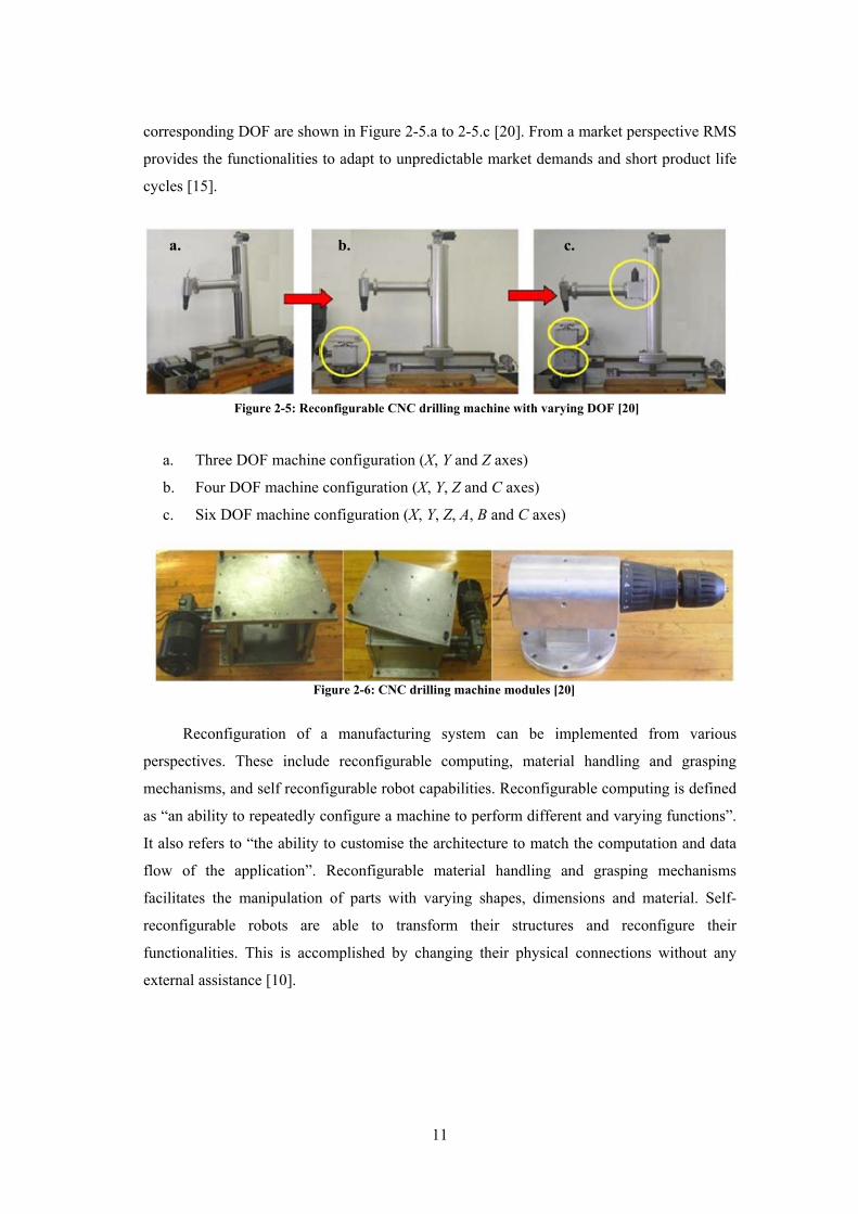
enhancement when introducing new methodologies [14]. Figure 2-5 [20] presents a

reconfigurable CNC drilling machine for a RMS. Configuring the machine with different or

added mechanical modules as circled in Figure 2-6 [20], enables a range of degrees of

freedom (DOF) to be available for part machining. The different machine setups with

11

corresponding DOF are shown in Figure 2-5.a to 2-5.c [20]. From a market perspective RMS

provides the functionalities to adapt to unpredictable market demands and short product life

cycles [15].

a. Three DOF machine configuration (X, Y and Z axes)

b. Four DOF machine configuration (X, Y, Z and C axes)

c. Six DOF machine configuration (X, Y, Z, A, B and C axes)

Reconfiguration of a manufacturing system can be implemented from various

perspectives. These include reconfigurable computing, material handling and grasping

mechanisms, and self reconfigurable robot capabilities. Reconfigurable computing is defined

as “an ability to repeatedly configure a machine to perform different and varying functions”.

It also refers to “the ability to customise the architecture to match the computation and data

flow of the application”. Reconfigurable material handling and grasping mechanisms

facilitates the manipulation of parts with varying shapes, dimensions and material. Self-

reconfigurable robots are able to transform their structures and reconfigure their

functionalities. This is accomplished by changing their physical connections without any

external assistance [10].

Figure 2-5: Reconfigurable CNC drilling machine with varying DOF [20]

c. b. a.

Figure 2-6: CNC drilling machine modules [20]

12

Utilising an RMS approach in a manufacturing environment provides many key

characteristics. These key characteristics can be implemented at software and hardware

levels, and can be summarised as follows [10, 14-15]:

Modularity: System modularity can comprise of software and hardware components.

Maintenance and upgrading by implementing a modular approach is easier and in

response lowers the life-cycle cost of a manufacturing system. Some of the key

advantages of utilising a modular approach includes reduced lead time, economies of

scale, increased product variety and product/component change. Easier product

diagnosis, maintenance and repair are also included.

Integrability: Integrability of a manufacturing cell is facilitated at a system, modular

and component level. It allows for future introduction of new technologies.

Integration of modules in a RMS environment is achieved quickly and accurately by

control, informational and mechanical interfaces which facilitates system

communication and integration.

Customisation: Customisation is the configuring of hardware, controls and system

capabilities that corresponds to the system architecture needed to facilitate the

manufacture of a specific product family. Utilising an open architecture approach,

assist in attaining the customised control. This customised control is accomplished

by integrating control modules that offer the required control functionalities for

manufacturing execution.

Diagnosability: It determines the efficiency of the system by applying monitoring

and reliability techniques.

Convertibility: Convertibility is the rapid changeover of a manufacturing system.

System changeover possesses short conversion times that facilitate quick

configuration and system adaptability for future products. From a technical and

resource perspective, convertibility may include rapid tuning of tools, fixtures,

software and raw material.

2.2.4 Comparison of Manufacturing Systems

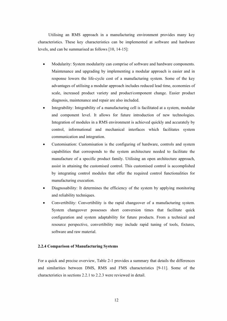
For a quick and precise overview, Table 2-1 provides a summary that details the differences

and similarities between DMS, RMS and FMS characteristics [9-11]. Some of the

characteristics in sections 2.2.1 to 2.2.3 were reviewed in detail.

13

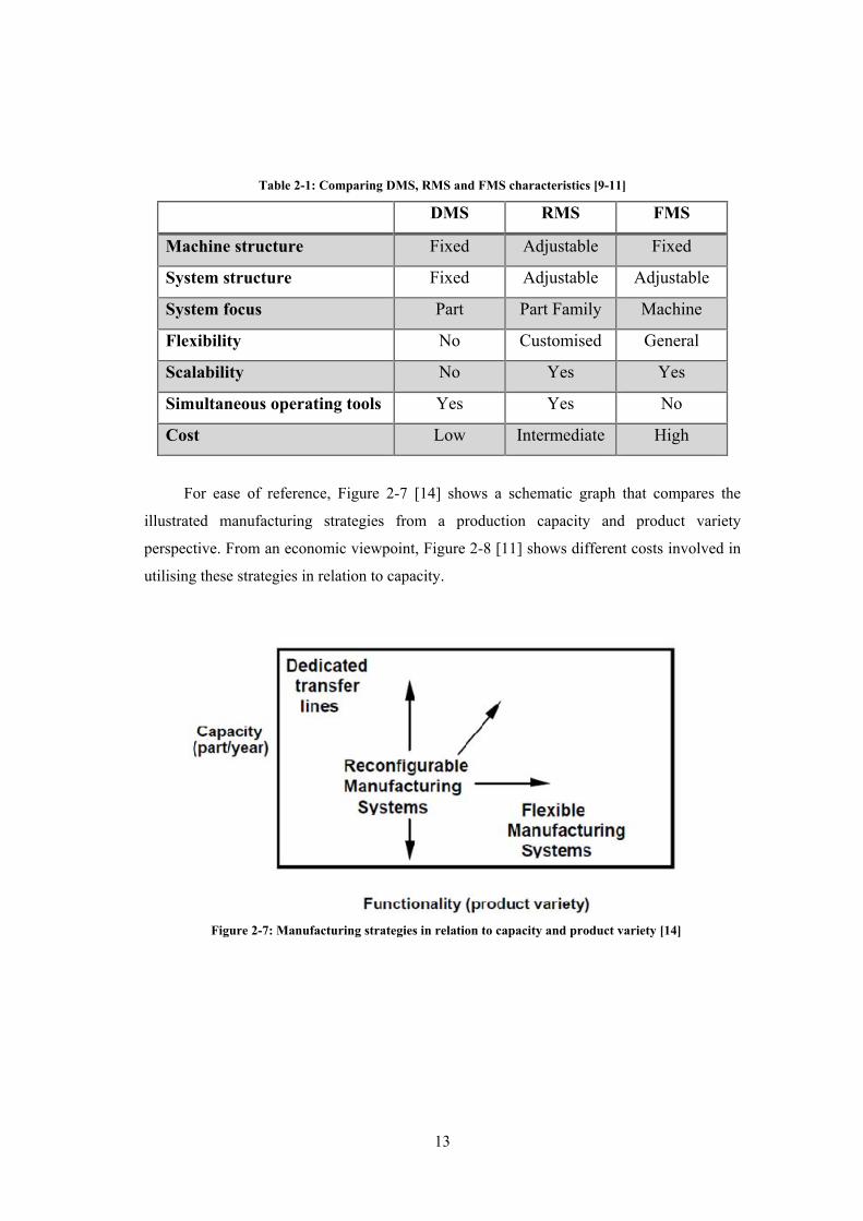
Figure 2-7: Manufacturing strategies in relation to capacity and product variety [14]

Table 2-1: Comparing DMS, RMS and FMS characteristics [9-11]

DMS RMS FMS

Machine structure Fixed Adjustable Fixed

System structure Fixed Adjustable Adjustable

System focus Part Part Family Machine

Flexibility No Customised General

Scalability No Yes Yes

Simultaneous operating tools Yes Yes No

Cost Low Intermediate High

For ease of reference, Figure 2-7 [14] shows a schematic graph that compares the

illustrated manufacturing strategies from a production capacity and product variety

perspective. From an economic viewpoint, Figure 2-8 [11] shows different costs involved in

utilising these strategies in relation to capacity.

14

2.2.5 Computer Integrated Manufacturing

A Computer Integrated Manufacturing approach is to completely automate a manufacturing

system [21]. CIM is the application of computer systems and its peripherals to aid in

production planning, executing information-processing functions, controlling operations and

designing products [8]. It is a manufacturing and fundamental management plan that

integrates manufacturing systems and facilities [22]. CIM incorporates the integration of

various advanced manufacturing operations. These include Computer-Aided Design (CAD),

Computer-Aided Manufacturing (CAM), Automated Material Handling, Computer

Numerical Control (CNC), Automated Storage and Retrieval Systems (ASRSs), and

Automated Guided Vehicles (AGVs) [23-27]. Figure 2-9 [28] illustrates some brief

applications of computer aided and managerial operations of a CIM system. Some of the

beneficial outcomes of implementing CIM include the following [21, 24]:

Reduces inventory levels.

Adapts to frequent production changes.

Figure 2-8: Manufacturing strategies in relation to capacity and system cost [11]

15

It possesses improved capabilities in contrast to other manufacturing strategies and

accommodates the production of intricate parts with high repeatability and accuracy.

Reduces manufacturing lead times.

Improves customer service.

It accommodates change for different product variety demands in a cost

effective manner without interrupting plant operations.

It provides increased flexibility.

Provides increased quality, speed and productivity.

2.3 Relevant Manufacturing Control and Automation Concepts

2.3.1 Hierarchy of Manufacturing Control and Automation

Automated systems can be divided into many levels of factory functionalities. Automation is

usually linked with individual production machines which contain subsystems that can also

be automated. As an example, this hierarchy concept of automation can be applied to modern

numerical control (NC) machine tools. The NC machine possesses multiple control systems

with varying amounts of motion axes (ranging from two to five axes) that operate as

Figure 2-9: Corresponding CIM functionalities [28]

16

positioning systems. These positioning systems are classified as automated systems. A NC

machine is an element of a larger manufacturing system. This larger manufacturing system

can itself be automated. Figure 2-10 [8] illustrates the hierarchy level for automated

production plants.

Following is a detailed description of the automation and control hierarchy for a

manufacturing environment [8]. The numbered list is in conjunction to the flow diagram

illustrated in Figure 2-10.

1. The device level is classified as the lowest level of automation. Sensors, actuators

and other low level hardware components form the device level. From a machine

perspective these devices are combined into the individual control loops. A single

joint of an industrial robot or one axis of a CNC machine is an example of a

feedback control loop.

Figure 2-10: Hierarchy of manufacturing control and automation [8]

17

2. Device level hardware is assembled to construct a machine. These include AGVs,

industrial robots, powered conveyors, CNC machine tools and related production

equipment.

3. This level is directly related to the manufacturing cell or system level. It functions in

coordination with plant level instructions. From an automation perspective, a

manufacturing cell or system can be defined as a group of workstations or machines.

In relation to this, these workstations or machines are supported and linked by a

computer, a material handling system and other equipment that conforms to the

manufacturing processes. The functionalities at this level incorporate part

dispatching and machine loading. In addition, synchronisation between machines

and material handling system is facilitated. Compiling and evaluation of inspection

data is also generated.

4. The plant level is the production system or factory level. At this level, instructions to

facilitate manufacturing procedures are executed. These instructions are initiated

from the business information system and include material requirements planning,

purchasing, order processing, shop floor control, quality control, inventory control

and process planning.

5. The enterprise level incorporates the business information system. Some of

functionalities that form this information system and simultaneously managers a

company include research, design, marketing and utilising a master production

schedule.

2.3.2 Intelligent Agent Based Approach for Manufacturing

An agent as defined by Wooldridge, is a computer system that is situated in some

environment, and is capable of autonomous action in this environment in order to meet its

design objectives [29].

Agents in the past were only implemented in software. However, modern available

state of technology and reconfigurable system makes it possible to adopt agent-based

techniques to configure hardware. This reconfigurable hardware can be configured in an

approach to best match its application. In some conditions this is done statically prior to

system execution and will remain unaffected during system operation. In other conditions,

the hardware can reconfigure dynamically during system operation and simultaneously

adjust to environmental system changes. This change in hardware configuration is in

18

response to demands being placed upon the system. A system may also be termed as hybrid,

where the collaboration of low-level hardware based agents and higher-level software agents

are used to attain the desired result [30].

From a software perspective, intelligent agents supply means of integrating various

manufacturing software applications. This integration is referred to as a multi-agent system

that is executed in a computer-based collaborative environment [31].

In a manufacturing environment, agent models are built and implemented in order

supply flexibility, reusability and fast response in cooperation with external and internal

uncertainties in the shop floor environment. Utilising agents in a dynamic manufacturing

system enriches the flexibility and reliability of the scheduling, and planning functions [32].

In order to be classified as an intelligent agent, it needs to be composed of various

properties. It should be reactive in terms of being responsive to changes in its environment,

proactive to achieve its goals, flexible in facilitating various techniques to achieve its goal

and robust in recovering from failure. In addition, it should be social in interacting with other

agents and autonomous in terms of behaving independently in an environment. An agent also

has to be rational in terms of its behaviour in an environment. Being rational will allow the

agent to make the correct decisions and be the most successful [29, 33].

At an elementary level, an intelligent agent can be thought of as anything that can

perceive its environment through sensors and act upon this environment through actuators.

As an example, a robot has cameras, infrared range finders as its sensors and motors as the

actuators. For each percept, a rational agent should select an action that is best suited to

maximise its performance from the series of built-in knowledge it possesses [30, 34]. This

defined functionality of an intelligent agent is illustrated in Figure 2-11 [30].

Figure 2-11: Diagram describing an agent [30]

19

2.4 Chapter Summary

This chapter provided a study of MC and the various manufacturing strategies that included

DMSs, FMSs, RMSs and CIM. It provided a comprehensive overview of each of strategy.

Furthermore, where required, it highlighted advantages and disadvantages of each strategy.

Collectively a comparison between DMSs, FMSs and RMSs was reviewed. From a

functional perspective, it presented an overview of the hardware and software related

techniques available for manufacturing control and automation.

20

3. HRCIM Cell Design Methodology

A methodology towards developing the HRCIM cell was directed by utilising specific design

approaches. RMS and FMS based characteristics were used to implement the HRCIM cell.

The conceptualised HRCIM cell consisted of hardware and software that incorporated

integrated functionality. This functionality facilitated coordinated hardware and software

behaviour that was generated by utilising specific design approaches. Existing resource

specifications initialised the bounds for HRCIM cell design and performance.

3.1 The Design Approach

To meet the required functionalities for modern or state-of-the-art manufacturing

environments, the HRCIM cell architecture was based on a mechatronic and basic intelligent

agent (see Chapter 2.3.2) design approach. Mechatronics can be defined from different

perspectives depending on the functionality it provides. In relation to the context of this

research, “Mechatronics is the synergistic integration of mechanical engineering with

electronic and electrical systems with intelligent computer control in the design and

manufacture of industrial products, processes and operations” [35]. Figure 3-1 [36] provides

an overview and brief examples of the mechatronic approach with its distributed interrelated

disciplinaries.

Figure 3-1: Diagram illustrating the mechatronic approach [36]

21

3.2 Conceptualising the HRCIM Cell

Existing manufacturing strategies as reviewed in Chapter 2.2, still require further

technological advancements to viably produce mass customised parts. These existing

strategies possess properties that are either too excessive or deficient.

From analysing the properties in Table 2-1, a DMS is too rigid in its machine and

system structure to introduce MC in its environment. Moreover, system architecture is

generally shaped around the type of part to be manufactured. From a RMS perspective, the

adjustable structure is built to provide just enough flexibility to manufacture parts within a

specified part family and therefore lacks the ability to support MC. FMSs which is based on

CIM technology [12], consists of fixed machine structures (CNC machine) with an

adjustable system structure that possesses remarkably high flexibility. This high flexibility

enables manufacturers to produce a great variety of customised parts but at low production

rates. A FMS with this high flexibility yields more setup time that result from programming

and adjusting system structure due to its ability to offer a large variety of custom parts.

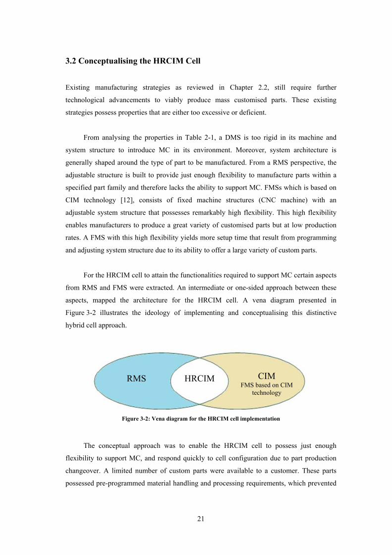
For the HRCIM cell to attain the functionalities required to support MC certain aspects

from RMS and FMS were extracted. An intermediate or one-sided approach between these

aspects, mapped the architecture for the HRCIM cell. A vena diagram presented in

Figure 3-2 illustrates the ideology of implementing and conceptualising this distinctive

hybrid cell approach.

The conceptual approach was to enable the HRCIM cell to possess just enough

flexibility to support MC, and respond quickly to cell configuration due to part production

changeover. A limited number of custom parts were available to a customer. These parts

possessed pre-programmed material handling and processing requirements, which prevented

Figure 3-2: Vena diagram for the HRCIM cell implementation

RMS HRCIM CIM FMS based on CIM

technology

22

added setup times. This conceptual approach introduced just enough flexibility and

reconfigurability into the HRCIM cell architecture. It fulfilled the prerequisites to support

MC, and reflected lower cost from a research perspective in contrast to high FMS cost.

The HRCIM cell being entirely computer controlled accommodated the integration of

intelligent agent based functionalities into the cell architecture. It provided the cell with an

intelligent based control system primarily from software functionalities. This approach

enabled synchronised functionalities of the cell components that promoted algorithm based

production scheduling and hardware reconfiguration for material handling purposes. The

HRCIM cell was created with integrated software and hardware, and its behaviour was

analysed using manufacturing software simulation procedures.

3.2.1 Hardware Architecture

The development of an efficient HRCIM cell with synchronised, compatible hardware

capabilities and infrastructure was restricted due to several constraints in the research

environment. The limited resources available and the high cost of modern manufacturing

equipment directed the development of the HRCIM cell that was economically feasible.

Designing and developing each of the equipment to a fully functional structure with the

required flexibility was not viable and relevant to the research. Conventional CIM methods

such as CAD and CAM were also not comprehensively applied in the cell. CAD was

indirectly performed in a simulation environment and results were captured for HRCIM cell

analysis. From a CAM viewpoint, only scheduling based manufacturing procedures were

conceptualised for HRCIM cell testing.

Existing hardware in the present manufacturing environment was refurbished and

optimised to form the HRCIM cell. Utilising this existing hardware, peak performance

measures of the manufacturing environment was not expected. Hardware that was vital and

not fully functional in the manufacturing cell was simulated by using its design and

performance specifications.

The HRCIM cell hardware consisted of device to machine level hardware. Highlighted

machine level hardware consisted of an ASRS, AGV, roller conveyors, CNC milling

machine and an Automated Modular Inspection Apparatus (AMIA). Among these, a

23

state-of-the-art, six axes Fanuc Robotic arm with reconfigurable end effectors and integrated

vision capabilities also formed the hardware architecture.

3.2.2 Software Architecture

From a software perspective, programming languages included Visual Basic (VB) and C.

The use of certain PC-based electronic control hardware also restricted the application of

certain programming languages. Visual basic was used to construct the Master Control

Program (MCP) for primary HRCIM cell activities. C was used has a secondary controller

for specific hardware applications. In addition, offline Fanuc based programming language

was used for robotic arm teaching. Integrated to this, and the functionality of producing

increased flexibility, a robot vision (iRvision) software package formed the intelligent

medium to link the robotic arm to the material handling system.

3.2.3 Software/Hardware Coordination

To synchronise software to hardware activities, digital electronic controllers specific to its

functionality formed the intermediate communication source. Certain digital controllers

(data acquisition boxes) operated dependently from PC support, whereas secondary digital

controllers (microcontrollers) operated independently from its own on-board processor. To

prevent any loss in digital transfer and feedback signals, the location of HRCIM cell

hardware was also bounded.

3.3 HRCIM Cell Specifications

The manufacturing cell architecture was developed according to the standard equipment

specifications tabulated in Table 3-1. Incompatibility between the listed hardware and

software, and restrictions in forming a real time closed loop manufacturing environment,

directed an approach towards extracting these standard specifications and simulating a fully

functional, integrated, synchronised HRCIM cell.

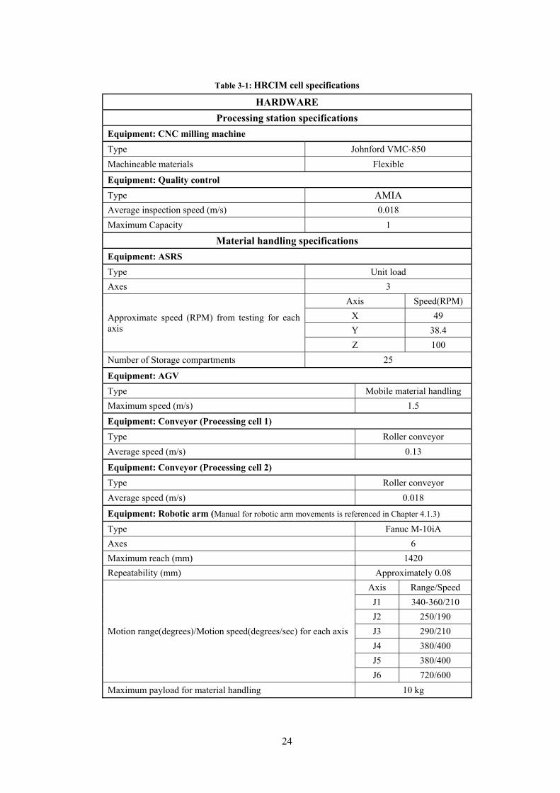
24

Table 3-1: HRCIM cell specifications

HARDWARE

Processing station specifications

Equipment: CNC milling machine

Type Johnford VMC-850

Machineable materials Flexible

Equipment: Quality control

Type AMIA

Average inspection speed (m/s) 0.018

Maximum Capacity 1

Material handling specifications

Equipment: ASRS

Type Unit load

Axes 3

Approximate speed (RPM) from testing for each axis

Axis Speed(RPM)

X 49

Y 38.4

Z 100

Number of Storage compartments 25

Equipment: AGV

Type Mobile material handling

Maximum speed (m/s) 1.5

Equipment: Conveyor (Processing cell 1)

Type Roller conveyor

Average speed (m/s) 0.13

Equipment: Conveyor (Processing cell 2)

Type Roller conveyor

Average speed (m/s) 0.018

Equipment: Robotic arm (Manual for robotic arm movements is referenced in Chapter 4.1.3)

Type Fanuc M-10iA

Axes 6

Maximum reach (mm) 1420

Repeatability (mm) Approximately 0.08

Motion range(degrees)/Motion speed(degrees/sec) for each axis

Axis Range/Speed

J1 340-360/210

J2 250/190

J3 290/210

J4 380/400

J5 380/400

J6 720/600

Maximum payload for material handling 10 kg

25

SOFTWARE continued

Operating system Windows XP

Programming languages C, Visual basic

G-code programming, part processing data for CNC EdgeCAM (Path simulator)

Robot vision software iRvision

ELECTRICAL

Main power supply (AC voltage) 220

DC power supply (DC voltage) 5, 12, 24

3.4 Chapter Summary

This chapter provided a brief background of the design approach that was used to construct

the HRCIM cell. It summarised the adverse aspects of implementing the reviewed

manufacturing strategies in accommodating MC. In response, it provided a build up towards

the development of the HRCIM cell. It also detailed the conceptual cell design architecture

from a hardware and software perspective. With respect to performance measures, a listed

specification for the utilised hardware and software was also provided.

26

4. Manufacturing Cell Design

The HRCIM cell architecture is composed of several manufacturing equipment. Material

handling platforms, buffer systems and processing stations form the bulk of the

manufacturing cell. To enable easy integration in the development of the cell architecture,

equipment was designed with homogeneous sizes and dimensions to facilitate an

uninterrupted flow of parts during production. The equipment was setup to provide a closed

loop production flow for simulation purposes.

To generate a well-defined overview, an assembled CAD model of the manufacturing

cell setup from two different viewpoints in space is presented in Figure 4-1.

Figure 4-1: HRCIM cell layout

2

107

6

5

9

4

3

1

8

12

11

14

13

27

Table 4-1 relates to equipment labelling in Figure 4-1. Figure 4-2 and Figure 4-3

respectively provides two views of the laboratory based manufacturing cell setup. Each

equipment as illustrated in Figure 4-1 is detailed further in Chapter 4.1 to 4.3.

Table 4-1: Equipment labelling in Figure 4-1

No: Equipment Name No: Equipment Name

1 PC 8 AMIA

2 ASRS 9 Fanuc robotic arm 1

3 AGV 10 Fanuc robotic arm 2

4 Circular conveyor (Conveyor 1) 11 Robotic arm vision camera

5 CNC machine 12 Robotic arm main controller

6 Intermediate buffer 13 Processing cell 1

7 Linear conveyor (Conveyor 2) 14 Processing cell 2

Figure 4-2: Physical cell setup - view 1

28

Figure 4-3: Physical cell setup - view 2

This setup facilitated and accommodated the manufacture of parts that contained specified

processing parameters. The available hardware functionalities and the HRCIM cell were

driven by these parts. Chapter 4.4 details the part library that was used to imitate MC. The

part flow overview is also defined.

4.1 Material Handling Platforms

4.1.1 Autonomous Guidance Vehicle for Process Integration

An existing Autonomous Guidance Vehicle as shown in Figure 4-4 [37] was used to map the

routing system for material handling purposes. The AGV provided a routing system from the

ASRS to the loading point of the conveyor as illustrated in Figure 4-14 [38]. The main

functionality of the AGV was to provide distributed process integration for closed loop cell

behaviour.

29

4.1.2 Conveyors

Existing roller conveyors were used to provide the platform for part loading and unloading.

A circular conveyor was used to serve the primary processing cell. To optimise its

functionality from an intelligent agent approach, a part detection sensor was incorporated to

its structure. This enabled asynchronous motion behaviour of the conveyor and in response

created a static platform for robotic arm part manipulation. For complex conveyor motion in

the event of added processing stations, more part detection sensors can be integrated along

the conveyor which will enable it to adapt to further manufacturing ideologies.

An existing linear conveyor was used to serve the secondary processing cell. Existing

configurations and data of the secondary manufacturing cell, gained from previous

research [39] was used to model a complete manufacturing cell that proved substantial to

meet the objectives of the present research.

4.1.3 Robotic Arm

Fanuc state-of-the-art, six axes, M-10iA series robotic arms (see Figure 4-5) was used to

perform complex material handling functionalities. The robotic arm was limited to its

movement in space as observed in Figure 4-6 [40].

Figure 4-4: AGV for HRCIM cell process integration [37]

30

Figure 4-5: Fanuc robotic arm

Figure 4-6: Robot restrictions in space [40]

31

At conceptual stages, initial end effector status provided no functionality to the

manufacturing cell as depicted in Figure 4-5. To provide a solution towards engaging mass

customisation, a reconfigurable end effector was developed to manipulate different part

geometries. This reconfigurable functionality was designed with interfaces which were

assembled with gripper modules. A detailed mechanical and electrical approach towards

developing this reconfigurable material handling robot is illustrated in Chapter 5.2.

As seen in Figure 4-1, robotic arm 1 (box 9), was used to serve the primary processing

cell. Primary processing cell activities included pick and place operations from the circular

conveyor to the CNC machine, and from the CNC machine to the intermediate buffer.

Robotic arm 2 was used to perform pick and place operations from the intermediate buffer to

the secondary processing cell. This enabled the seamless flow of work in process from the

primary to secondary manufacturing cell.

The robotic arm main controller was also integrated with vision capabilities. An

infrared camera placed above the circular conveyor system, provided feedback of part arrival

and initiated actions for robotic arm part manipulation. The robot vision system also served

to provide the added flexibility and functionality for the robotic arm. Integrated vision

functionalities were only applied to robotic arm 1.

Due to economical constraints, reconfigurable end effector design was not applied to

robotic arm 2. Vision capabilities were not viable to implement in robotic arm 2 due to the

absence of a mechanical end effector manipulator. The robotic arm was however

programmed to imitate the pick and place events from the intermediate buffer to the AMIA

machine, and return to its home position from the AMIA to the intermediate buffer. This

assumption facilitated the summation of robotic arm 2 material handling time which was

used to parameterise the manufacturing simulation.

4.2 Buffer Systems

4.2.1 Automated Storage and Retrieval System

A unit load Automated Storage and Retrieval System (see Figure 4-7) was used to serve the

material handling system with parts. This existing unit load system performs handling of

pallet stored parts. Its previous control system was composed of dilapidated components and

32

mechanisms. Modern electronic devices were used to improve the ASRS’s precision and

efficiency. In response to applying complex functionalities, the ASRS was developed to be

fully automated, computer controlled and be entirely integrated with manufacturing

operations [8].

The use of an ASRS in this research was primarily to form a structured arrangement of

parts and to investigate its behaviour with software scheduling operations in response to

customer order input. Movement of the ASRS crane was based on three axes, consisting of

linear x, y and z movements as depicted in Figure 4-8. Each axis operated independently with

respect to its linear movement. The destination point to retrieve a part was directly dependent

on the scheduling of customer orders. To validate this random retrieval of parts, four storage

points were used to form an inventory for the four part types (see Chapter 4.4) available for

processing. As observed in Figure 4-9, the storage points are numerically listed. With

reference to Figure 4-10, storage points 1-4 represented part types A, B, C and D

respectively.

Figure 4-7: ASRS

Crane

33

Figure 4-8: ASRS coordinates

Reference point

Figure 4-9: ASRS storage points

Unloading zone

34

4.2.2 Intermediate Buffer

A buffer was placed between processing cell one and two. It formed an intermediate storage

point that linked both processing cells and facilitated the synchronous flow of work in the

process. Its horizontal structure in space provided an accurate operational space for robotic

arm part manipulation between the processing cells.

4.3 Processing Stations

4.3.1 CNC Machine

The absence of a functional, modern CNC machine in the UKZN manufacturing laboratory

did not meet the specifications for the HRCIM cell hardware nor could it provide data for

simulation purposes. Using the Johnford VMC-850 CNC milling machine (see Figure 4-10)

that was external to the laboratory, part processing times was simulated by utilising offline

integrated CAM software (EdgeCam). This approach made it possible to acquire results

based from actual CNC cutting speeds and tool changeover times.

Figure 4-10: Johnford VMC-850 CNC milling machine

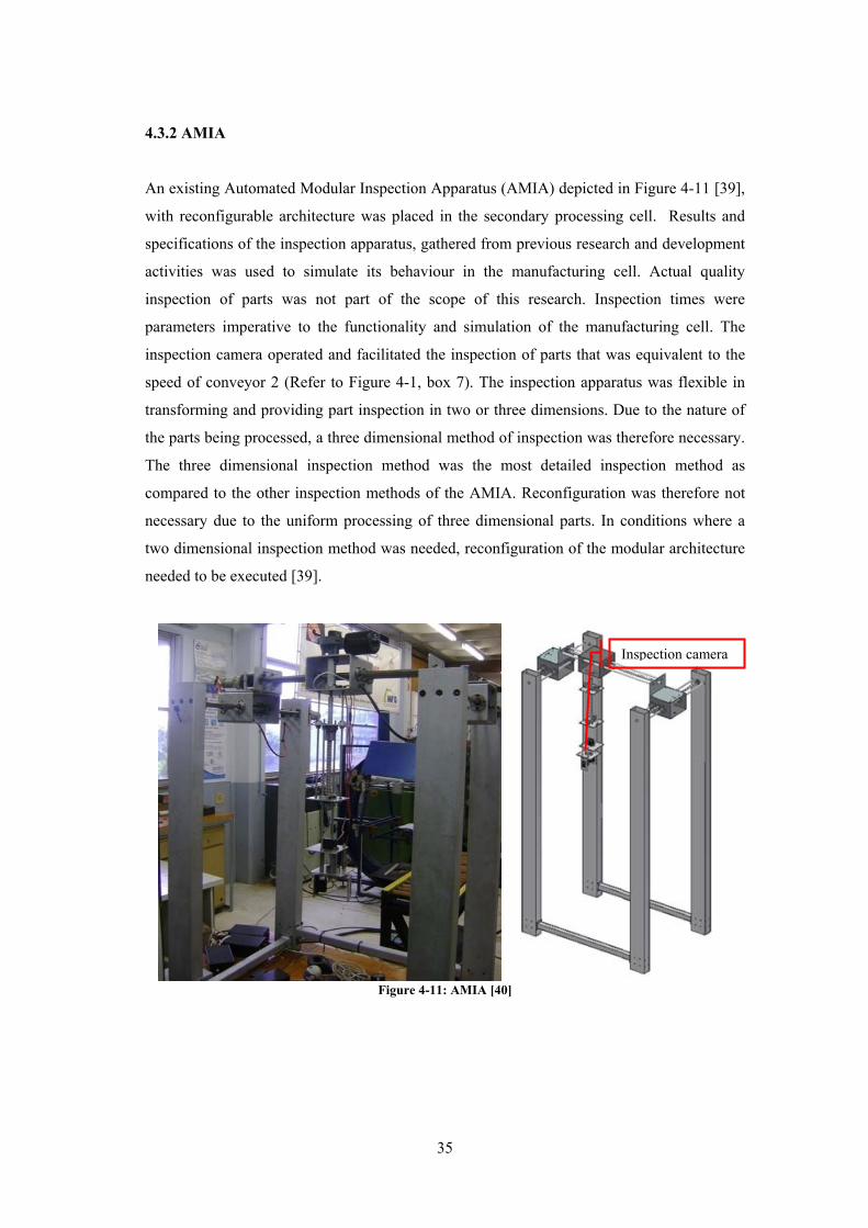
35

4.3.2 AMIA

An existing Automated Modular Inspection Apparatus (AMIA) depicted in Figure 4-11 [39],

with reconfigurable architecture was placed in the secondary processing cell. Results and

specifications of the inspection apparatus, gathered from previous research and development

activities was used to simulate its behaviour in the manufacturing cell. Actual quality

inspection of parts was not part of the scope of this research. Inspection times were

parameters imperative to the functionality and simulation of the manufacturing cell. The

inspection camera operated and facilitated the inspection of parts that was equivalent to the

speed of conveyor 2 (Refer to Figure 4-1, box 7). The inspection apparatus was flexible in

transforming and providing part inspection in two or three dimensions. Due to the nature of

the parts being processed, a three dimensional method of inspection was therefore necessary.

The three dimensional inspection method was the most detailed inspection method as

compared to the other inspection methods of the AMIA. Reconfiguration was therefore not

necessary due to the uniform processing of three dimensional parts. In conditions where a

two dimensional inspection method was needed, reconfiguration of the modular architecture

needed to be executed [39].

Figure 4-11: AMIA [40]

Inspection camera

36

4.4 Part Library and Flow

4.4.1 Part Library

The list of parts to drive and substantiate the manufacturing process is depicted in

Figure 4-12. The parts were chosen according to the definition of MC. Following this

definition, Part A and B had similar geometries but contained different machining

parameters. This same concept was applied to Part C and D. These parts were introduced

randomly into the HRCIM cell for processing and created a discrete environment for

HRCIM cell behaviour.

Due to limitations within the research environment to process these parts,

geometrically based components were used to imitate these parts as shown in Figure 4-13.

Component A represented Part A and B, component B represented Part C and D. The mass

of the components were not to exceed the maximum robot material handling payload of 10

kilograms as specified in Table 3-1. Component A and B respectively possessed masses of

24.21 and 15.92 grams, which were exceedingly within limits of the maximum allowable

payload.

PART A PART B

PART C PART D

Figure 4-12: Library of parts

Figure 4-13: Substitution for part type

37

4.4.2 Part Flow

The library of parts or components used, possessed a homogeneous part flow. Figure 4-14

contains an overview of the HRCIM cell part flow.

4.5 Chapter Summary

This chapter provides an overview of the equipment used, and details the functionality of

each, with respect to the HRCIM cell specifications and architecture. Where necessary,

limitations of certain equipment were declared. The part catalogue and part flow used to

drive the HRCIM cell is also provided.

Part flow

ASRSAGVConveyor 1Robot 1Robot 2Conveyor 2

Figure 4-14: Part flow

38

Figure 5-1: Vision camera support platform.

Camera

Camera support

platform

5. Mechanical Design

The mechanical design consisted of modifying and assembling existing or new mechanical

hardware. Majority of the design was in the development of new mechanical hardware that

was imperative to meet specifications required by the HRCIM cell. Moreover, it provided the

rigid platform for the vision and tooling capabilities. These mechanical designs in addition,

projected an augmented reconfigurable and flexible manufacturing cell environment. It also

provided a platform to enable the sophisticated cell functionalities to be achieved.

5.1 Mechanical Support Structure for the Robot Vision Camera

The 2D vision camera was integrated with the robot main controller and provided feedback

for part detection along the material handling conveyor system. This camera provided the

robot vision capabilities and was mechanically fixed in the manufacturing cell. Initial

calibrated location of the camera in space was stored. Any minor variations from the initial

calibration point rendered incorrect robot pick and place points. To prevent this, the camera

was attached to a rigid support frame (see Figure 5-1). Preferably the support frame is most

effective when it is rigidly grounded.

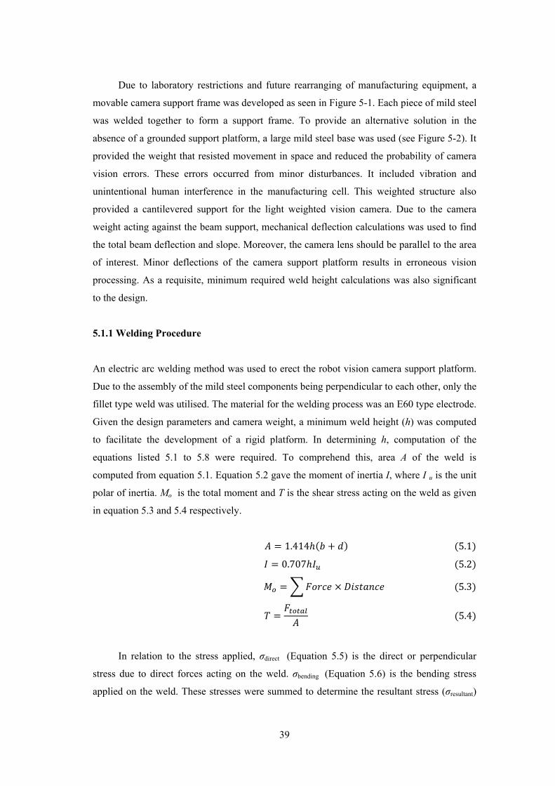
39

Due to laboratory restrictions and future rearranging of manufacturing equipment, a

movable camera support frame was developed as seen in Figure 5-1. Each piece of mild steel

was welded together to form a support frame. To provide an alternative solution in the

absence of a grounded support platform, a large mild steel base was used (see Figure 5-2). It

provided the weight that resisted movement in space and reduced the probability of camera

vision errors. These errors occurred from minor disturbances. It included vibration and

unintentional human interference in the manufacturing cell. This weighted structure also

provided a cantilevered support for the light weighted vision camera. Due to the camera

weight acting against the beam support, mechanical deflection calculations was used to find

the total beam deflection and slope. Moreover, the camera lens should be parallel to the area

of interest. Minor deflections of the camera support platform results in erroneous vision

processing. As a requisite, minimum required weld height calculations was also significant

to the design.

5.1.1 Welding Procedure

An electric arc welding method was used to erect the robot vision camera support platform.

Due to the assembly of the mild steel components being perpendicular to each other, only the

fillet type weld was utilised. The material for the welding process was an E60 type electrode.

Given the design parameters and camera weight, a minimum weld height (h) was computed

to facilitate the development of a rigid platform. In determining h, computation of the

equations listed 5.1 to 5.8 were required. To comprehend this, area A of the weld is

computed from equation 5.1. Equation 5.2 gave the moment of inertia I, where I u is the unit

polar of inertia. Mo   is the total moment and T is the shear stress acting on the weld as given

in equation 5.3 and 5.4 respectively.

1.414                                                 5.1

  0.707                                                             5.2

                               5.3

                                                                 5.4

In relation to the stress applied, σdirect (Equation 5.5) is the direct or perpendicular

stress due to direct forces acting on the weld. σbending (Equation 5.6) is the bending stress

applied on the weld. These stresses were summed to determine the resultant stress (σresultant)

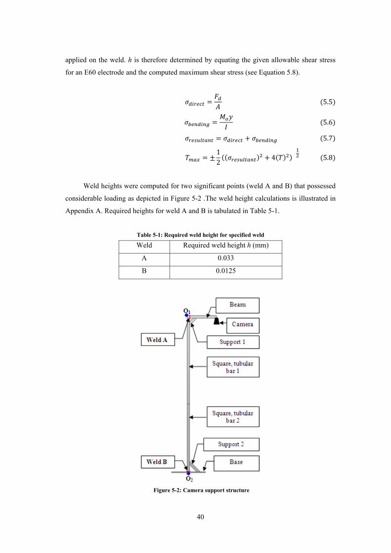
40

applied on the weld. h is therefore determined by equating the given allowable shear stress

for an E60 electrode and the computed maximum shear stress (see Equation 5.8).

                                                              5.5

                                                       5.6

                            5.7

1

24

                      5.8

Weld heights were computed for two significant points (weld A and B) that possessed

considerable loading as depicted in Figure 5-2 .The weld height calculations is illustrated in

Appendix A. Required heights for weld A and B is tabulated in Table 5-1.

Table 5-1: Required weld height for specified weld

Weld Required weld height h (mm)

A 0.033

B 0.0125

Figure 5-2: Camera support structure

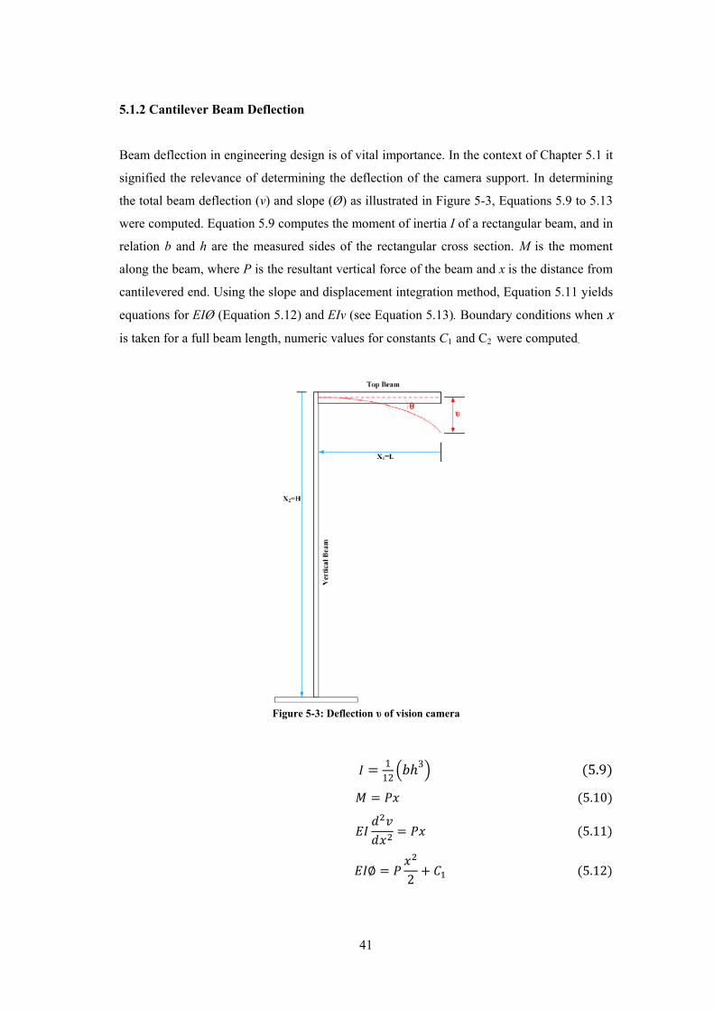
41

5.1.2 Cantilever Beam Deflection

Beam deflection in engineering design is of vital importance. In the context of Chapter 5.1 it

signified the relevance of determining the deflection of the camera support. In determining

the total beam deflection (v) and slope (Ø) as illustrated in Figure 5-3, Equations 5.9 to 5.13

were computed. Equation 5.9 computes the moment of inertia I of a rectangular beam, and in

relation b and h are the measured sides of the rectangular cross section. M is the moment

along the beam, where P is the resultant vertical force of the beam and x is the distance from

cantilevered end. Using the slope and displacement integration method, Equation 5.11 yields

equations for EIØ (Equation 5.12) and EIv (see Equation 5.13). Boundary conditions when x  

is taken for a full beam length, numeric values for constants C1  and C2  were computed. 

  

 

 

    1

12

3                                                 5.9

                                                              5.10

                                                     5.11

∅2

                                              5.12

Figure 5-3: Deflection υ of vision camera

42

                                   5.13

Appendix B provides the calculations that compute the total deflection of the camera.

The total deflection υ determined was 0.64 millimetres. This deflection was diminutive and

in response did not produce any erroneous vision processing errors.

5.2 Reconfigurable Robotic Arm End Effector

Mechanical design of the reconfigurable robotic arm gripper included the assembly of

components with interface plates. The actuation of this assembled module was attained by

utilising pneumatic electromechanical devices that facilitated the reconfigurable end effector

behaviour. The design was based on key RMS characteristics which entailed modularity,

integrability, customisation and convertibility. These characteristics with respect to Chapters

5.2 and 5.3 are elaborated as follows.

Modularity provided an approach to increase product variety and enable product

change within the manufacturing cell.

Integrability provided the flexibility to introduce new end effector modules for

robotic arm material handling or processing.

Customisation enabled robot end effector configuration to generate the manufacture

of a particular product.

Convertibility provided quick changeover of the robot end effector for adaptability

of future products.

5.2.1 End Effector Interfaces

The robotic arm end effector was supplied with fixed dimensions for fastener attachment.

These dimensions were used to attach a SCHUNK quick-change head with a bolted

aluminium interface plate as shown in Figure 5-4. This quick-change head formed a common

connection point for each gripper module (see Figures 5-5 and 5-6). The 2-finger parallel

gripper module (see Figure 5-5) was used to perform material handling on square part

geometries, whereas the 3-finger centric gripper module (see Figure 5-6) performed material

handling on circular part geometries. This ideology was used to represent a discrete part

geometry flow in response to MC. Each module consisted of a SCHUNK quick-change

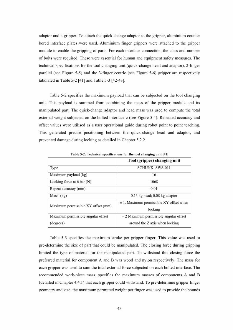
43

adaptor and a gripper. To attach the quick change adaptor to the gripper, aluminium counter

bored interface plates were used. Aluminium finger grippers were attached to the gripper

module to enable the gripping of parts. For each interface connection, the class and number

of bolts were required. These were essential for human and equipment safety measures. The

technical specifications for the tool changing unit (quick-change head and adaptor), 2-finger

parallel (see Figure 5-5) and the 3-finger centric (see Figure 5-6) gripper are respectively

tabulated in Table 5-2 [41] and Table 5-3 [42-43].

Table 5-2 specifies the maximum payload that can be subjected on the tool changing

unit. This payload is summed from combining the mass of the gripper module and its

manipulated part. The quick-change adaptor and head mass was used to compute the total

external weight subjected on the bolted interface c (see Figure 5-4). Repeated accuracy and

offset values were utilised as a user operational guide during robot point to point teaching.

This generated precise positioning between the quick-change head and adaptor, and

prevented damage during locking as detailed in Chapter 5.2.2.

Table 5-2: Technical specifications for the tool changing unit [41]

Tool (gripper) changing unit

Type SCHUNK, SWS-011

Maximum payload (kg) 16

Locking force at 6 bar (N) 1068

Repeat accuracy (mm) 0.01

Mass (kg) 0.13 kg head; 0.08 kg adapter

Maximum permissible XY offset (mm) ± 1, Maximum permissible XY offset when

locking

Maximum permissible angular offset

(degrees)

± 2 Maximum permissible angular offset

around the Z axis when locking

Table 5-3 specifies the maximum stroke per gripper finger. This value was used to

pre-determine the size of part that could be manipulated. The closing force during gripping

limited the type of material for the manipulated part. To withstand this closing force the

preferred material for component A and B was wood and nylon respectively. The mass for

each gripper was used to sum the total external force subjected on each bolted interface. The

recommended work-piece mass, specifies the maximum masses of components A and B

(detailed in Chapter 4.4.1) that each gripper could withstand. To pre-determine gripper finger

geometry and size, the maximum permitted weight per finger was used to provide the bounds

44

prior to its design. The unlocking/locking functionality between the quick-change head and

adaptor is detailed in Chapter 5.2.2.

Table 5-3: Technical specifications for the grippers [42-43]

2-finger parallel

gripper

3-finger centric

gripper

Type JGP 64-1 JGZ 64-1

Stroke per finger (mm) 6 6

Closing force (N) 250 580

Opening force (N) 270 640

Mass (kg) 0.28 0.43

Recommended work-piece mass (kg) 1.25 2.9

Minimum/Maximum operating pressure (bar) 2.5/8 2/8

Nominal operating pressure (bar) 6 6

Closing/Opening time (seconds) 0.03/0.03 0.03/0.03

Maximum permitted weight per finger (kg) 0.35 0.35

Repeat accuracy (mm) 0.01 0.01

Figure 5-4: Interface c for quick-change head attachment

Quick-change head

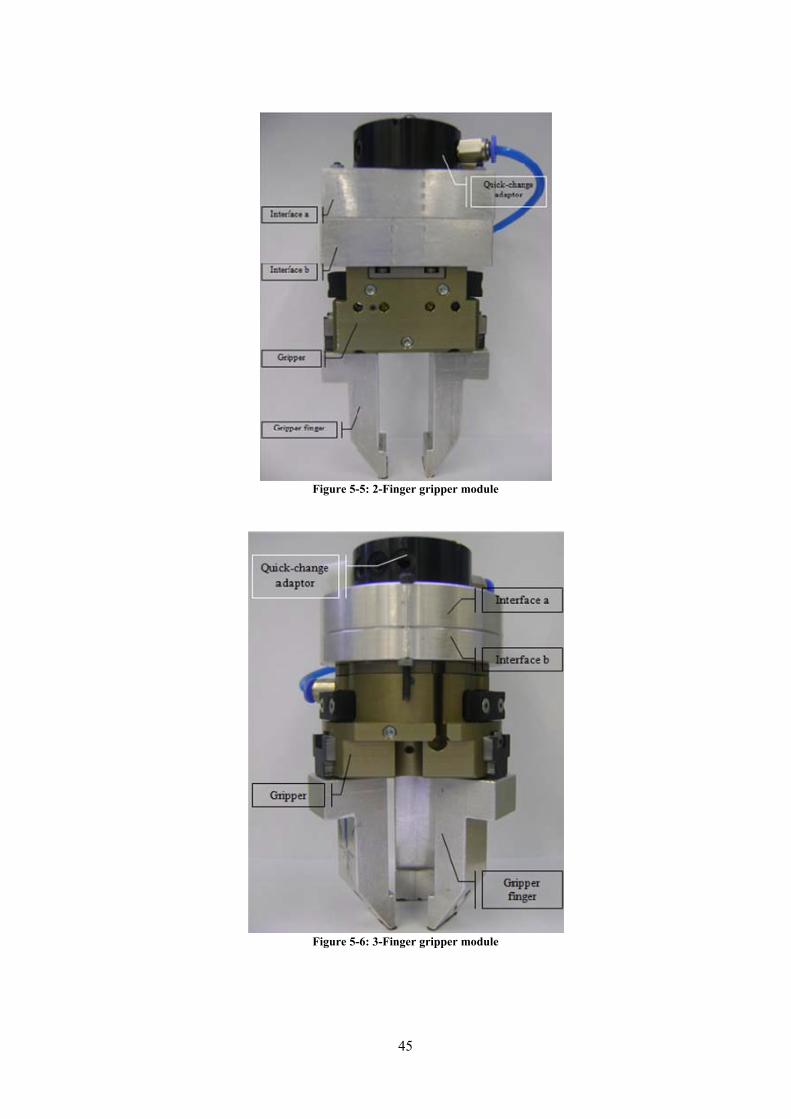
45

Figure 5-6: 3-Finger gripper module

Figure 5-5: 2-Finger gripper module

46

5.2.1.1 Interface Requirements

In response to high speed and vibration caused during robotic arm movements, interface

failure was a significant preventative factor. Formulated approaches (Equation 5.14 - 5.21) in

establishing thread shear, joint separation, tightening torque and maximum shear stress

provided a directed approach for effective interfacing. Equation 5.14 determines the bolt

tensile load (F) required to cause thread-stripping of the nut material, where d is the bolt

diameter, t is the nut thickness and SSY is the shear yield strength. Nut material was taken as

aluminium, with the exception of a carbon steel nut material for the end effector. Fi is the

initial tensile force required and is dependent on the standard tensile stress area of the bolt

(At), the proof strength (Sp) and the constant Ki as shown in equation 5.15. Ki was assumed to

be a value of 0.9 for static loading operations due to insignificant loading and operation

times. Equations 5.16-5.17 give the tightening torque (T) and the clamped area (Ac)

respectively, where g is the clamped length.

πd 0.75t S                                            5.14

                                                       5.15

0.2                                                          5.16

0.68 0.065                       5.17

The joint separation force (Fe) required to separate a bolted interface is given by

equation 5.18. It is computed from Kb which is the bolt stiffness and Kc which is the interface

stiffness. Eb and Ec is the modulus of elasticity for the bolt and interface material

respectively, and was used to determine Kb and Kc in equation 5.19-5.20. The maximum

shear force (Fs) required for bolt failure is illustrated in Figure 5.21. It has minor adverse

effects as the gripper modules are rarely subjected to significant shear forces. A is the cross

sectional area of the bolt that was used to calculate this maximum shear force.

                                                 5.18

                                                         5.19

                                                          5.20

                                                       5.21

47

The calculated bolt tensile force (F), joint separation force (Fe), recommended

tightening torque (T) and maximum shear force (Fs) is computed in Appendix C. These were

computed for the interfaces labelled in Figure 5-4 to 5-6. These results are listed in Table 5-4

to Table 5-6.

Table 5-4: Calculated results for interface failure

Interface name

Total bolt

tensile force F,

(N)

Total joint

separation

force Fe, (N)

Recommended

tightening

torque T, (N.m)

Maximum

shear force Fs,

(N)

c 37310.81 27411.6 4 8017.34

Table 5-5: Calculated results for 2-finger gripper interfaces

Interface name

for 2-finger

gripper

Total bolt

tensile force F,

(N)

Total joint

separation

force Fe, (N)

Recommended

tightening

torque T, (N.m)

Maximum

shear force Fs,

(N)

a 13529.27 35133 12.4 12527.1

b 18039 37170 12.4 12527.1

a+b 41489.76 19047.5 2.63 4509.76

Table 5-6: Calculated results for 3-finger gripper interfaces

Interface name

for 2-finger

gripper

Total bolt

tensile force

F, (N)

Total joint

separation

force Fe, (N)

Recommended

tightening

torque T, (N.m)

Maximum

shear force

Fs, (N)

a 9019.5 39947.75 12.4 125271.1

b 37881.95 108508.2 21.06 18039.03

a and b 31117.32 14936.1 2.63 4509.76

Table 5-7 lists the subjected external weight and the joint separation force for each

bolted interface. The subjected weight as tabulated is excessively lower than the force

required for joint separation. Part weight was trivial during gripper manipulation and was

therefore neglected in computing the weight acting against the bolted interfaces.

48

Table 5-7: Joint separation force in comparison to the external weight subjected

Interface Subjected weight (N) Fe (N)

c 12.5 27411.6

2-Finger parallel gripper

Interface Subjected weight (N) Fe (N)

a 7.55 35133

b 3.5 37170

a+b 7.55 19047.5

3-Finger centric gripper

Interface Subjected weight (N) Fe (N)

a 10 39947.75

b 5.77 108508.2

a+b 10 14936.1

5.2.2 End Effector Actuation

To provide the locking and unlocking actuation for gripper module selection and facilitate

the gripping of objects, pneumatic solenoid valves were used. The gripper actuation was

achieved by the intake of compressed air that was sustained from an approximate 8bar main

air supply source. Opening and closing of solenoid valves were facilitated by 24 volt digital

electrical logic signals. The digital electrical signals were sourced from the robot I/O port

pins as illustrated in Chapter 6.2.3. Solenoid valves were positioned on the robotic arm as

illustrated in Figure 5-7.

Two types of valves were used to facilitate the reconfigurable functionality of the end

effector. A Pneumax 5/2 way valve (see Figure 5-8), actuated from a solenoid coil (labelled a

in Figure 5-8) and spring return was used to lock and unlock the quick-change adaptor from

the quick-change head. For actuation to be facilitated a minimum working pressure of 2.5 bar

was required [44]. Figure 5-9 presents a logic flow diagram for this electromechanical

operation. Locking enables the docking of a gripper module and unlocking enables the

undocking of a gripper module from the tool (gripper) holding table.

49

For finger gripping actuation, a Festo 5/3 way solenoid valve (see Figure 5-8)

actuated from a double solenoid coil (labelled b and c in Figure 5-8) was utilised. For

actuation to be accomplished a minimum working pressure of 3 bar was necessitated [45].

Figure 5-10 presents a logic flow diagram for opening and closing of the gripper finger.

Figure 5-8 illustrates the flow of air when either of the solenoid coils is energised by a

24 volt digital electrical signal. The colour coded lines represents the flow of air when either

of the solenoid coils are energised. Figure 5-9 and Figure 5-10 provides the logic diagram

with matching colour symbols that are in relation to Figure 5-8.

Figure 5-7: Solenoid valve setup on the robotic arm

Quick-change

head

Motor

Robotic arm

5/2 way

solenoid valve

5/3 way

solenoid valve

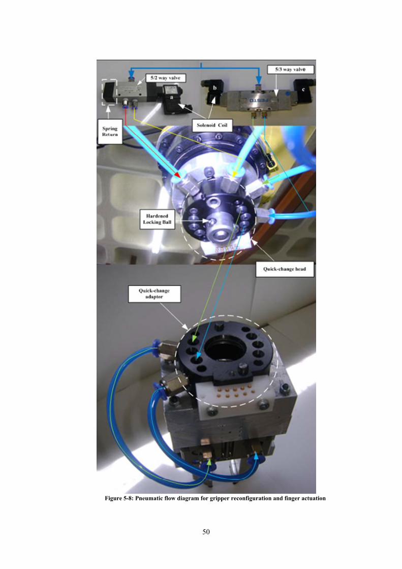
50

Figure 5-8: Pneumatic flow diagram for gripper reconfiguration and finger actuation

51

Figure 5-9: 5/2 way solenoid valve logic diagram

52

Figure 5-10: 5/3 way solenoid valve logic diagram

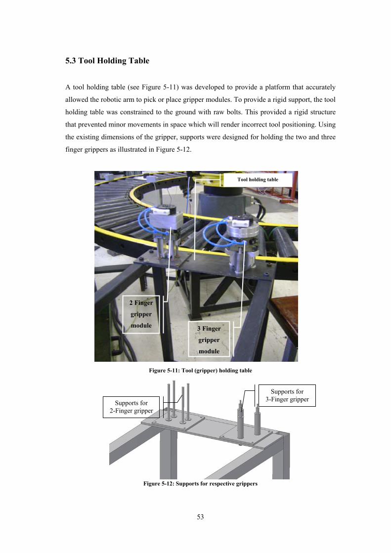
53

5.3 Tool Holding Table

A tool holding table (see Figure 5-11) was developed to provide a platform that accurately

allowed the robotic arm to pick or place gripper modules. To provide a rigid support, the tool

holding table was constrained to the ground with raw bolts. This provided a rigid structure

that prevented minor movements in space which will render incorrect tool positioning. Using

the existing dimensions of the gripper, supports were designed for holding the two and three

finger grippers as illustrated in Figure 5-12.

Figure 5-12: Supports for respective grippers

Supports for 3-Finger gripper

Supports for 2-Finger gripper

2 Finger

gripper

module 3 Finger

gripper

module

Tool holding table

Figure 5-11: Tool (gripper) holding table

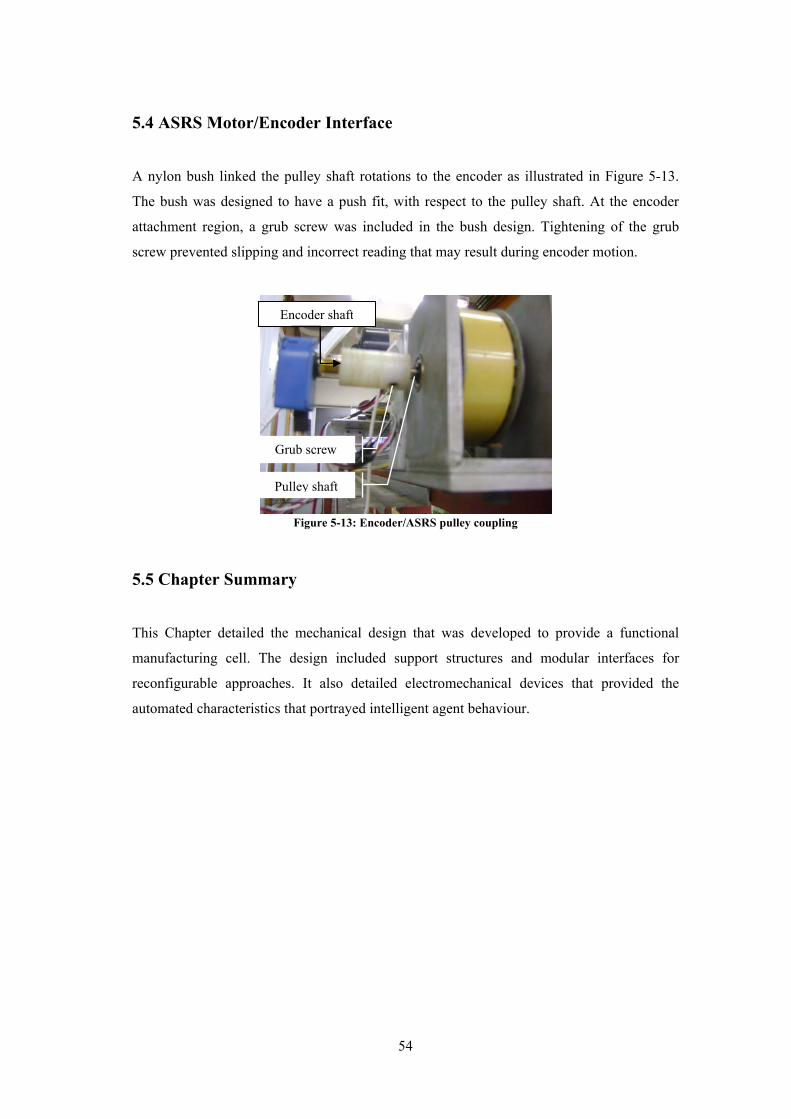
54

5.4 ASRS Motor/Encoder Interface

A nylon bush linked the pulley shaft rotations to the encoder as illustrated in Figure 5-13.

The bush was designed to have a push fit, with respect to the pulley shaft. At the encoder

attachment region, a grub screw was included in the bush design. Tightening of the grub

screw prevented slipping and incorrect reading that may result during encoder motion.

5.5 Chapter Summary

This Chapter detailed the mechanical design that was developed to provide a functional

manufacturing cell. The design included support structures and modular interfaces for

reconfigurable approaches. It also detailed electromechanical devices that provided the

automated characteristics that portrayed intelligent agent behaviour.

Pulley shaft

Grub screw

Encoder shaft

Figure 5-13: Encoder/ASRS pulley coupling

55

6. Electronic Design

Electronic applications facilitated the integration between the mechanical and software

architecture. It provided seamless integration for synchronised and coordinated functionality

between the manufacturing cell equipment. In relation to intelligent agent methodologies,

specific electronic devices were used to sense changes in the manufacturing cell and

consequently reacted to these changes. Electronic devices that comprised of more flexible

and sophisticated functionality were used for intermediary and master manufacturing cell

control.

6.1 Device Level Electronic Applications

6.1.1 Light Dependent Resistor

Detection of moving parts at a fixed point along the circular conveyor was facilitated by a

Light Dependent Resistor (LDR) as shown in Figure 6-1. A laser diode served as the LDRs

source of light. Focusing the laser diode on the LDR facilitated conveyor movement.

Detection of parts which obstructed this channel of light halted conveyor movement. The

stationary conveyor provided a platform for robotic arm vision and part manipulation. It

prevented erroneous vision processing results that may result in incorrect robot positioning

for part picking operations.

Laser diode

Enclosed LDR circuit

Part to be

processed

Enclosed laser diode

Figure 6-1: LDR setup

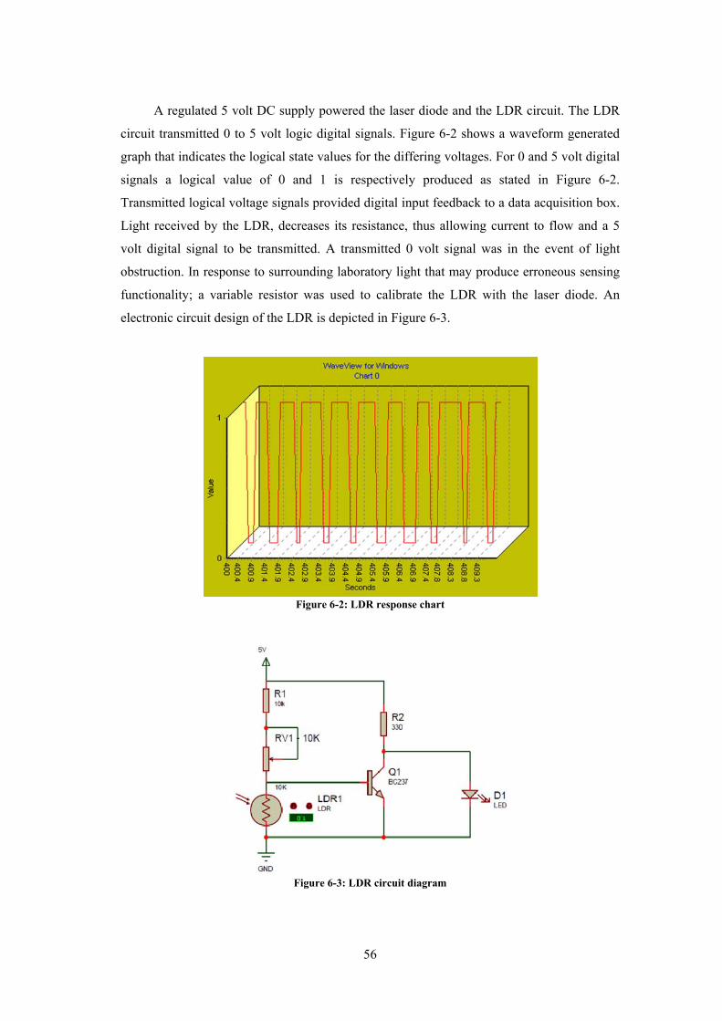
56

A regulated 5 volt DC supply powered the laser diode and the LDR circuit. The LDR

circuit transmitted 0 to 5 volt logic digital signals. Figure 6-2 shows a waveform generated

graph that indicates the logical state values for the differing voltages. For 0 and 5 volt digital

signals a logical value of 0 and 1 is respectively produced as stated in Figure 6-2.

Transmitted logical voltage signals provided digital input feedback to a data acquisition box.

Light received by the LDR, decreases its resistance, thus allowing current to flow and a 5

volt digital signal to be transmitted. A transmitted 0 volt signal was in the event of light

obstruction. In response to surrounding laboratory light that may produce erroneous sensing

functionality; a variable resistor was used to calibrate the LDR with the laser diode. An

electronic circuit design of the LDR is depicted in Figure 6-3.

Figure 6-3: LDR circuit diagram

Figure 6-2: LDR response chart

57

6.1.2 Encoders

HEDS-5700 optical incremental shaft encoders as depicted in Figure 6-4 were attached to

each ASRS pulley axis. This is also shown in Figure 5-13. It provided the position control

for the ASRS crane. The encoder with labelled colour coded wires is illustrated in

Figure 6-4. A 5 volt DC supply, regulated from an ASRS axis microcontroller powered the

encoder. Channel A (Pin 3) was used for incremental counting during rotational movement

of the encoder shaft. For this functionality, use of Channel B in conjunction with Channel A

was not required. Concurrently these channels are used for quadrature incremental output.

Rotation of the encoder transmitted pulses along Channel A to the interrupt pin of an ASRS

axis microcontroller [46].

Operational features of the encoder included an allowable maximum speed of 2000

RPM and it possesses 256 cycles per revolution from channel A [46]. Computations from

experimental procedures resulted in different linear distances for one encoder revolution of

an ASRS axis (see Appendix D.1). Discrepancies resulted from DC motors being subjected

to different magnitudes of load from the crane. Table 6-1 includes the calculated results for

the approximate linear distance per encoder revolution.

Figure 6-4: Encoder with wiring colour code table [46]

58

Table 6-1: ASRS crane distance per encoder revolution

Approximate linear distance per revolution

Axis Distance (mm)

X 249.5

Y 244.6

Z 309.7

6.1.3 Limit Switches

Each end of the X and Z ASRS axis consisted of a limit switch that provided the fixed

bounds for crane movement. Restrictions within the Y axis design only accommodated a

single limit switch. The limit switches prevented the stalling of motors and damage to the

mechanical structure of the ASRS. A 5 volt DC supply from the ASRS axis microcontroller

was used as the input to the limit switch. Contact of the ASRS crane with the limit switch

transmitted a 5 volt logic signal to the specified port C pin of the microcontroller. When the

pin received this signal, switching of the relay took place and concurrently impeded motor

and crane movement.

5 Volt high from microcontoller

Vcc pin

Normally Open. Signal to

input pin of microcontroller

Figure 6-5: Limit switch

59

6.1.4 Relays to Control ASRS Crane Movement

The utilised 15 Amp relay circuit consisted of an augmented reverse polarity. Its architecture

provided the forward motion, reverse motion and stationary state for the ASRS crane. Each

ASRS axis consisted of a relay that switched the DC motor to the corresponding states. A 15

Amp relay sufficiently accommodated a single motor and provided a margin for increased

motor load. The relay circuit also comprised of a 15 Amp fuse that terminated relay

functionality in the event of motor overload. A 12 volt DC supply was used to power the

relay circuit and in the event of an input logic signal, the DC motor was powered. The input

logic signals were transmitted from an intermediate controller (see Chapter 6.2.1). The

values were of 0 or 5 volt logic. A 0 volt digital logic signal impeded motor motion. In the

event of a 5 volt digital logic signal, the motor was driven. To facilitate the reverse motor

motion, a 5 volt logic signal was applied concurrently to inputs A and B (see Figure 6-6). To

illustrate these functionalities graphically, Figure 6-6 depicts and labels the mentioned

applications.

Common Ground

Normally Open

12 V Battery +

12 Volt Battery -

Common Ground

Power Supply to Motor -

Power Supply to Motor +

Ground

Input from µDAQ

Input from µDAQ for Reverse

Polarity

+ 12 Volt Power Supply

Fuse

Figure 6-6: 15 Amp relay circuit

A B

60

6.1.5 Relays to Control Circular Conveyor Movement

Two 30 Amp relay circuits were used to control the four DC motors that drove the roller

conveyors. It provided the unidirectional motion and stationary conveyor states. Each relay

circuit sufficiently accommodated two DC motors without any overload. A 12 volt DC

supply was used to power the relay circuit. In receiving an input digital logic signal the 12

volt DC supply simultaneously powered the DC motor. The input logic signals were of 0 or 5

volt logic and were transmitted from an Eagle µDAQLite (see Chapter 6.2.2) data acquisition

box. A 0 volt digital logic signal impeded motor motion and a 5volt digital logic signal

provided motor motion. Figure 6-7 shows a labelled 30 Amp relay circuit used to facilitate

conveyor motion.

6.1.6 A Step-up Voltage Logic Circuit

The different incompatible HRCIM cell controllers generated or required prescribed digital

voltages to render cell activities. Different logic voltage values existed, particularly from the

- 12 V Power Supply +

- Motor +

- 12 V Power supply +µDAQlite Ground µDAQlite 0 or 5 Volt DC logic

signal

Figure 6-7: 30 Amp relay circuit

61

5 volt digital logic signals generated from the µDAQLite (see Chapter 6.2.2) and the 24 volt

digital logic value required by the robotic arm input port pins for part manipulation. The

µDAQLite transmitted 0 or 5 volt logic signals in response to LDR part detection. To

provide an integrated approach in response to these voltage values, a 5/24 volt digital step-up

logic circuit was developed. It coordinated the µDAQLite 0 or 5 volt logic output signals to

the 24 volt digital input signals required by the robotic arm (see Chapter 6.2.3) input port

pin.

Utilising this step-up logic circuit provided a systematic and seamless part logistic

behaviour along the circular conveyor system. It enabled correct part positioning results to be

generated by permitting the visual capture of parts subsequent to LDR part detection.

Following part detection and with an added delay time, robotic arm part manipulation was

initiated and corresponded precisely to part location.

Figure 6-8: 5/24 volt step up logic circuit

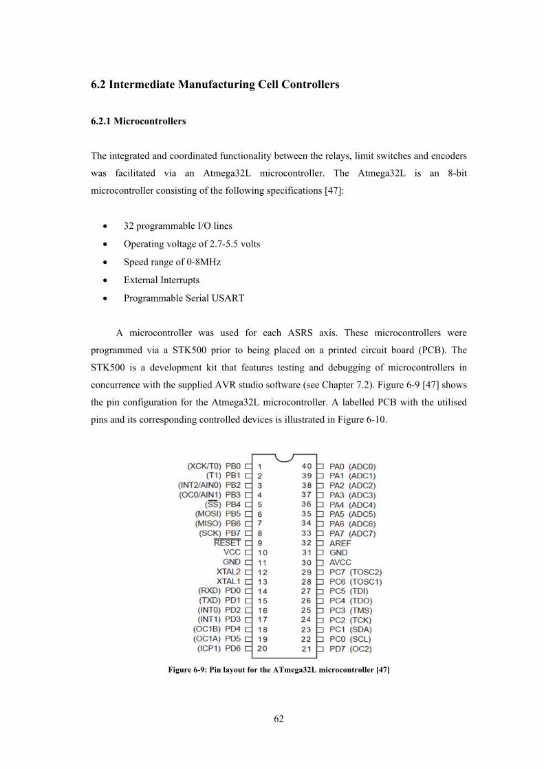
62

6.2 Intermediate Manufacturing Cell Controllers

6.2.1 Microcontrollers

The integrated and coordinated functionality between the relays, limit switches and encoders

was facilitated via an Atmega32L microcontroller. The Atmega32L is an 8-bit

microcontroller consisting of the following specifications [47]:

32 programmable I/O lines

Operating voltage of 2.7-5.5 volts

Speed range of 0-8MHz

External Interrupts

Programmable Serial USART

A microcontroller was used for each ASRS axis. These microcontrollers were

programmed via a STK500 prior to being placed on a printed circuit board (PCB). The

STK500 is a development kit that features testing and debugging of microcontrollers in

concurrence with the supplied AVR studio software (see Chapter 7.2). Figure 6-9 [47] shows

the pin configuration for the Atmega32L microcontroller. A labelled PCB with the utilised

pins and its corresponding controlled devices is illustrated in Figure 6-10.

Figure 6-9: Pin layout for the ATmega32L microcontroller [47]

63

Depicted in Figure 6-10, pull down resistors were used to compensate for the voltage

float experienced. This voltage float occurred in reaction to the opened state of the limit

switch (see Figure 6-5). When the limit switch was closed, it provided a 5 volt digital logic

input to the microcontroller. Once the switch was opened, a 0 volt digital logic input was

expected in response to the floating 5 volt digital logic experienced. This produced

inconsistent ASRS crane movements.

This identical voltage float was also evident from the Eagle µDAQ data acquisition

box (see Chapter 6.3) input signals during operation. This occurred during signal changeover

from an approximate 5 to 0 volt digital logic state. With reference to Figure 6-10, a solution

whereby pull down resistors between the corresponding pin and ground was connected to

prevent this voltage float.

PA1PA0 PA2

PA3

PA5

PA6

PA7

PA4PB0

PB1

PD2

PC

1

PC

0

Gro

und

Ground

Ground

12 V Supply Voltage

Pul

l dow

n re

sist

or

Atmega 32L Microcontroller

Vcc

Figure 6-10: PCB for Atmega32L microcontroller

64

6.2.1.1 Universal Asynchronous Receiver/Transmitter

Utilising the Universal Asynchronous Receiver/Transmitter (USART) feature of the

Atmega32L microcontroller enabled data to be transmitted during the testing and

development phase of the ASRS. Received data via PC was not relevant to the development.

Transmitted data was initiated from the microcontroller. It provided programming assistance

and calibration for the ASRS crane. A USB-SERIAL interface connector, depicted in

Figure 6-11 [48], facilitated this data transfer from the USART to the PC USB port. Data

buffered contained the incremented encoder pulses that resulted from ASRS axis motion.

Figure 6-11 illustrates the pin configuration for the USB-SERIAL interface connector. A 5

volt DC supply from the Atmega32L powered this device. The STX pin was used to transfer

USART data to the PC USB port. This transmitted data was analysed via the PC

HyperTerminal software. For efficient and legible data transfer a baud rate of 4800, and a

clock speed of 1 MHz was utilised [48].

6.2.2 Data Acquisition Control

A USB powered, PC supported Eagle µDAQLite data acquisition box, as shown in

Figure 6-12 [49], received and transmitted signals in order to facilitate material handling

activities. The µDAQLite consisted of eight input and output channels that respectively

received or transmitted 0 or 5 volt digital logic signals. Input channels were used to

accommodate the signals generated from the LDR circuit (see Chapter 6.1.1) during part

detection. The output channels transmitted signals to the 30 Amp relays (see Chapter 6.1.5)

for driving or halting conveyor movement. Halting conveyor movement during part

detection transmitted a 5 volt digital output logic signal for robotic arm part manipulation.

Figure 6-11: USB-serial interface connector [48]

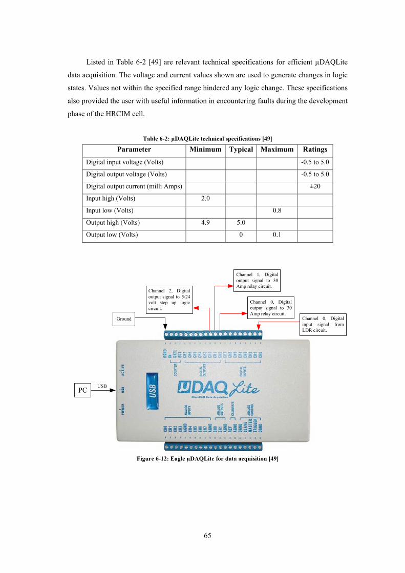
65

Listed in Table 6-2 [49] are relevant technical specifications for efficient µDAQLite

data acquisition. The voltage and current values shown are used to generate changes in logic

states. Values not within the specified range hindered any logic change. These specifications

also provided the user with useful information in encountering faults during the development

phase of the HRCIM cell.

Table 6-2: µDAQLite technical specifications [49]

Parameter Minimum Typical Maximum Ratings

Digital input voltage (Volts) -0.5 to 5.0

Digital output voltage (Volts) -0.5 to 5.0

Digital output current (milli Amps) ±20

Input high (Volts) 2.0

Input low (Volts) 0.8

Output high (Volts) 4.9 5.0

Output low (Volts) 0 0.1

Channel 0, Digital input signal from LDR circuit.

Ground

Channel 2, Digital output signal to 5/24 volt step up logic circuit.

Channel 1, Digital output signal to 30 Amp relay circuit.

Channel 0, Digital output signal to 30 Amp relay circuit.

PCUSB

Figure 6-12: Eagle µDAQLite for data acquisition [49]

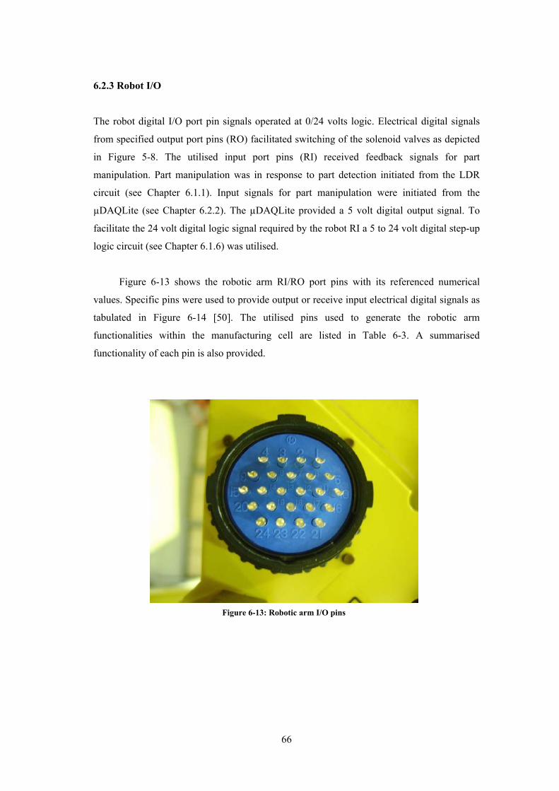
66

6.2.3 Robot I/O

The robot digital I/O port pin signals operated at 0/24 volts logic. Electrical digital signals

from specified output port pins (RO) facilitated switching of the solenoid valves as depicted

in Figure 5-8. The utilised input port pins (RI) received feedback signals for part

manipulation. Part manipulation was in response to part detection initiated from the LDR

circuit (see Chapter 6.1.1). Input signals for part manipulation were initiated from the

µDAQLite (see Chapter 6.2.2). The µDAQLite provided a 5 volt digital output signal. To

facilitate the 24 volt digital logic signal required by the robot RI a 5 to 24 volt digital step-up

logic circuit (see Chapter 6.1.6) was utilised.

Figure 6-13 shows the robotic arm RI/RO port pins with its referenced numerical

values. Specific pins were used to provide output or receive input electrical digital signals as

tabulated in Figure 6-14 [50]. The utilised pins used to generate the robotic arm

functionalities within the manufacturing cell are listed in Table 6-3. A summarised

functionality of each pin is also provided.

Figure 6-13: Robotic arm I/O pins

67

Table 6-3: Robot I/O pin description and functionality

Pin number at robotic arm end

effector interface (RI/RO)

Robotic

arm

I/O pin

Functionality

1 RO1

Output 24 Volt signal to solenoid

coil c of the 5/3 way pneumatic

valve (see Figure 5-8)

2 RO2

Output 24 Volt signal to solenoid

coil b of the 5/3 way pneumatic

valve (see Figure 5-5)

4 RO4

Output 24 Volt signal to solenoid

coil a of the 5/2 way pneumatic

valve (see Figure 5-5)

9 RI1

Receives 0/24 Volt DC input for

robot image processing in response

to LDR part detection

23 0 V Ground

6.3 Master Manufacturing Cell Controller

An Eagle µDAQ digital I/O data acquisition box with 120 digital I/O lines was used as the

master HRCIM cell controller [51]. This data acquisition box was specifically chosen as it

comprised of numerous I/O lines to support the HRCIM cell requirements. To meet these

requirements only the output lines were utilised. These output lines was used to transmit

signals to the ASRS microcontrollers. The output signals were generated from a scheduling

algorithm (see Chapter 7.1) that mapped the ASRS axis movements for part retrieval.

Figure 6-14: Pin layout for end effector interface (RI/RO) [50]

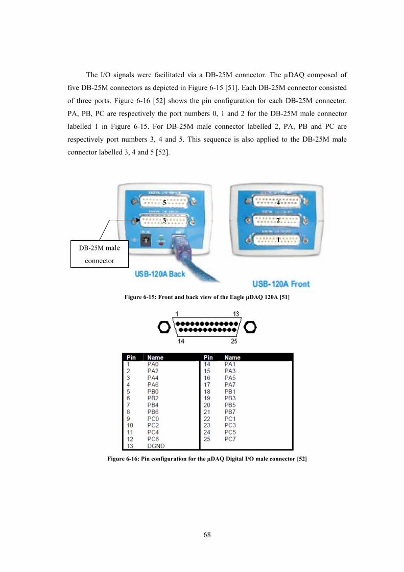
68

The I/O signals were facilitated via a DB-25M connector. The µDAQ composed of

five DB-25M connectors as depicted in Figure 6-15 [51]. Each DB-25M connector consisted

of three ports. Figure 6-16 [52] shows the pin configuration for each DB-25M connector.

PA, PB, PC are respectively the port numbers 0, 1 and 2 for the DB-25M male connector

labelled 1 in Figure 6-15. For DB-25M male connector labelled 2, PA, PB and PC are

respectively port numbers 3, 4 and 5. This sequence is also applied to the DB-25M male

connector labelled 3, 4 and 5 [52].

Figure 6-16: Pin configuration for the µDAQ Digital I/O male connector [52]

Figure 6-15: Front and back view of the Eagle µDAQ 120A [51]

1

2

4

3

5

DB-25M male

connector

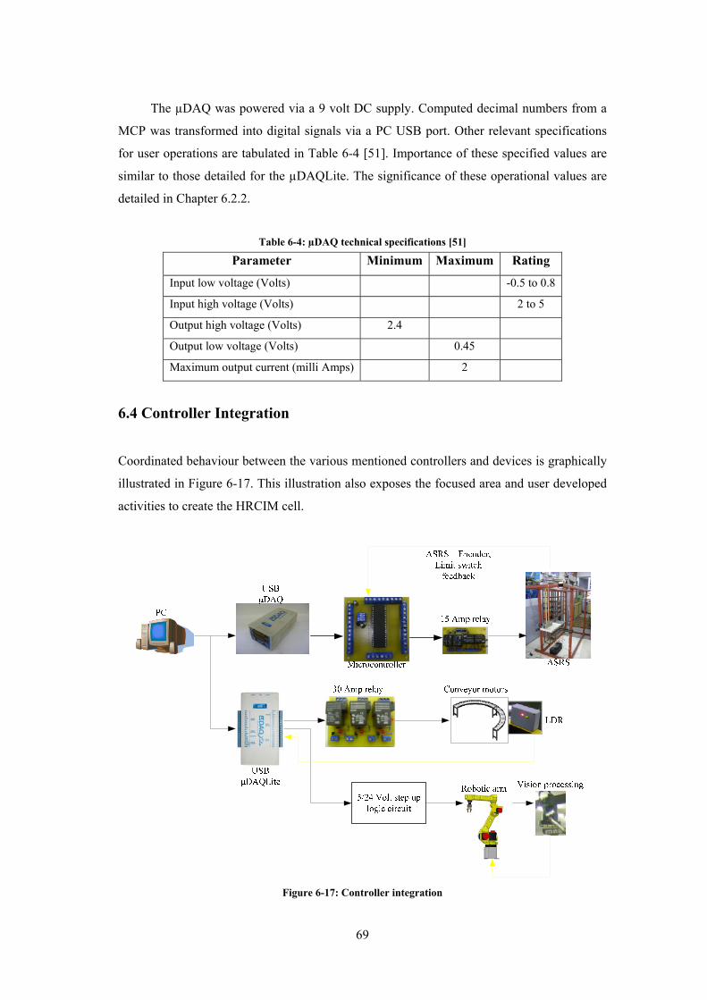
69

The µDAQ was powered via a 9 volt DC supply. Computed decimal numbers from a

MCP was transformed into digital signals via a PC USB port. Other relevant specifications

for user operations are tabulated in Table 6-4 [51]. Importance of these specified values are

similar to those detailed for the µDAQLite. The significance of these operational values are

detailed in Chapter 6.2.2.

Table 6-4: µDAQ technical specifications [51]

Parameter Minimum Maximum Rating

Input low voltage (Volts) -0.5 to 0.8

Input high voltage (Volts) 2 to 5

Output high voltage (Volts) 2.4

Output low voltage (Volts) 0.45

Maximum output current (milli Amps) 2

6.4 Controller Integration

Coordinated behaviour between the various mentioned controllers and devices is graphically

illustrated in Figure 6-17. This illustration also exposes the focused area and user developed

activities to create the HRCIM cell.

Figure 6-17: Controller integration

70

A comprehensive overview that maps the controller pins to certain activities for ASRS

position control is tabulated in Table 6-5. This flow of activities was in response to a high

logic level (5 Volt DC). Device level feedback to specific microcontroller pins is also listed

in Table 6-6. Highlighted columns signify the use of a pull down resistor as explained in

Chapter 6.2.1 and depicted in Figure 6-10.

Control from the µDAQLite data acquisition box was not coordinated with the µDAQ

data acquisition box. Utilised µDAQLite pins and its related functionality at a logic high are

mapped in Table 6-7. Vision processing from the 2D vision camera was coordinated with

LDR logic states. This coordinated behaviour is also tabulated in Table 6-7.

Table 6-5: Coordinated and synchronised controller behaviour at logic high

USB μDAQ Output (Port

Number ; Pin

Number)

→ Input to

Microcontroller (Pin)

→ Microcontroller

Output →

Motor direction, driven by 15A Relay

Circuit

→ ASRS Position

ASRS - X Axis Control (Storage points are incremented along the X axis)

(0 ; 0) → PA0 → PB0 → Forward → Move to storage point 1

(0 ; 1) → PA1 → PB0 → Forward → Move to storage point 2

(0 ; 2) → PA2 → PB0 → Forward → Move to storage point 3

(0 ; 3) → PA3 → PB0 → Forward → Move to storage point 4

(0 ; 4) → PA4 → PB0 → Forward → Move to storage point 5

(0 ; 5) → PA5 → PB0 & PB1 → Reverse → Reverse to reference point

(0 ; 6) → PA6 → PB0 → Forward → Move to drop off point

(0 ; 7) → PA7 → Reset pin values

ASRS - Y Axis Control (Storage points are incremented along the Y axis)

(3 ; 0) → PA0 → PB0 → Forward → Move to storage point 1

(3 ; 1) → PA1 → PB0 → Forward → Move to storage point 2

(3 ; 2) → PA2 → PB0 → Forward → Move to storage point 3

(3 ; 3) → PA3 → PB0 → Forward → Move to storage point 4

(3 ; 4) → PA4 → PB0 → Forward → Move to storage point 5

(3 ; 5) → PA5 → PB0 & PB1 → Reverse → Reverse to reference point

(3 ; 6) → PA6 → Reset pin values

(3 ; 7) → PA7 → PB0 → Forward → Lift pallet

ASRS - Z Axis Control

(6 ; 0) → PA0 → PB0 → Forward

Move towards storage point

(6 ; 1) → PA1 → PB0 & PB1 → Reverse Reverse to reference point

(6 ; 2) → PA2 → PB0 & PB1 → Reverse Move to drop off point

(6 ; 3) → PA3 → Reset pin values

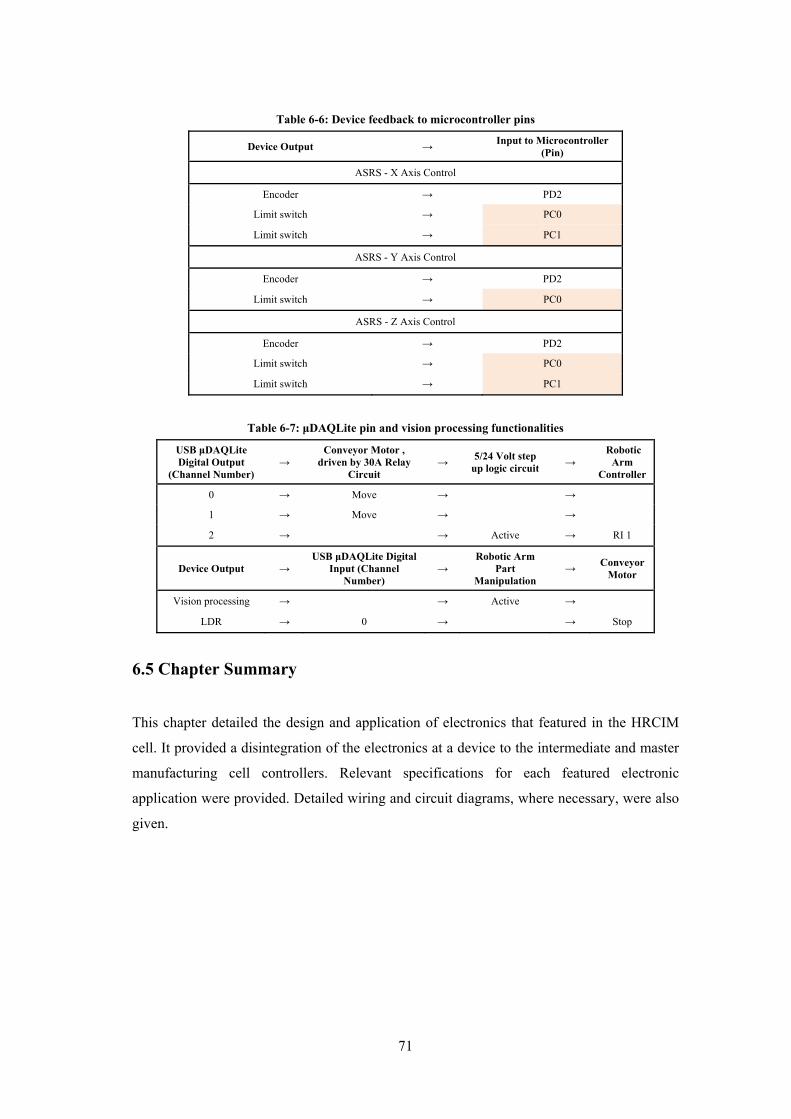
71

Table 6-6: Device feedback to microcontroller pins

Device Output → Input to Microcontroller

(Pin)

ASRS - X Axis Control

Encoder → PD2

Limit switch → PC0

Limit switch → PC1

ASRS - Y Axis Control

Encoder → PD2

Limit switch → PC0

ASRS - Z Axis Control

Encoder → PD2

Limit switch → PC0

Limit switch → PC1

Table 6-7: μDAQLite pin and vision processing functionalities

USB μDAQLite Digital Output

(Channel Number) →

Conveyor Motor , driven by 30A Relay

Circuit →

5/24 Volt step up logic circuit

→ Robotic

Arm Controller

0 → Move → →

1 → Move → →

2 → → Active → RI 1

Device Output → USB μDAQLite Digital

Input (Channel Number)

→ Robotic Arm

Part Manipulation

→ Conveyor

Motor

Vision processing →    → Active →

LDR → 0 →    → Stop

6.5 Chapter Summary

This chapter detailed the design and application of electronics that featured in the HRCIM

cell. It provided a disintegration of the electronics at a device to the intermediate and master

manufacturing cell controllers. Relevant specifications for each featured electronic

application were provided. Detailed wiring and circuit diagrams, where necessary, were also

given.

72

7. Software Design

Software related design or applications were subsequent to three programming languages.

The selection of a programming language was dependent upon the utilised electronic

controllers. Visual Basic and C programming languages were used to customise the

manufacturing cell requirements accordingly. Teaching of the robotic arm was subsequent to

utilising the integrated programming language incorporated within the Fanuc main

controller. Supplementary software included the robotic vision package (iRvision) that

assisted in supplying added flexibility to the HRCIM cell.

7.1 Featured Visual Basic Applications

The Master Control Program (MCP) was created from the Visual Basic 6 framework. Key

functionalities of the MCP included algorithm originated intelligent priority scheduling for

input of customer orders. The algorithm was based on computing a coefficient of priority for

each customer order. The lower the coefficient of priority, the higher priority that specific

order had to be processed [33].

Equation 8.1 and 8.2 was used to compute these priority values, where Pi is the number

of parts per order, PTp is the CNC machine processing time per part and PTo is the time to

produce an order. Tf is the time till due date and Cpriority is the coefficient of priority [33].

Results based on these equations are listed in Table 8-1. A complete VB code used to

formulate this scheduling algorithm is illustrated in Appendix E.2.

                              8.1

                              8.2

The MCP made use of an Application Programming Interface (API) provided with the

Eagle technology data acquisition boxes. The API enabled the data acquisition

functionalities to be coordinated with the MCP. Each part to be processed consisted of an

arrangement of API write functions (EDRE_DioWrite) as denoted in Figure 7-1. As shown,

cbbserial is the Eagle data acquisition box serial number, txtportwrite is the port number and

txtvaluewrite is the user defined decimal number that represents which ports pins should be

active [53]. Table 7-1 provides a few examples of applying a logic high (active) for

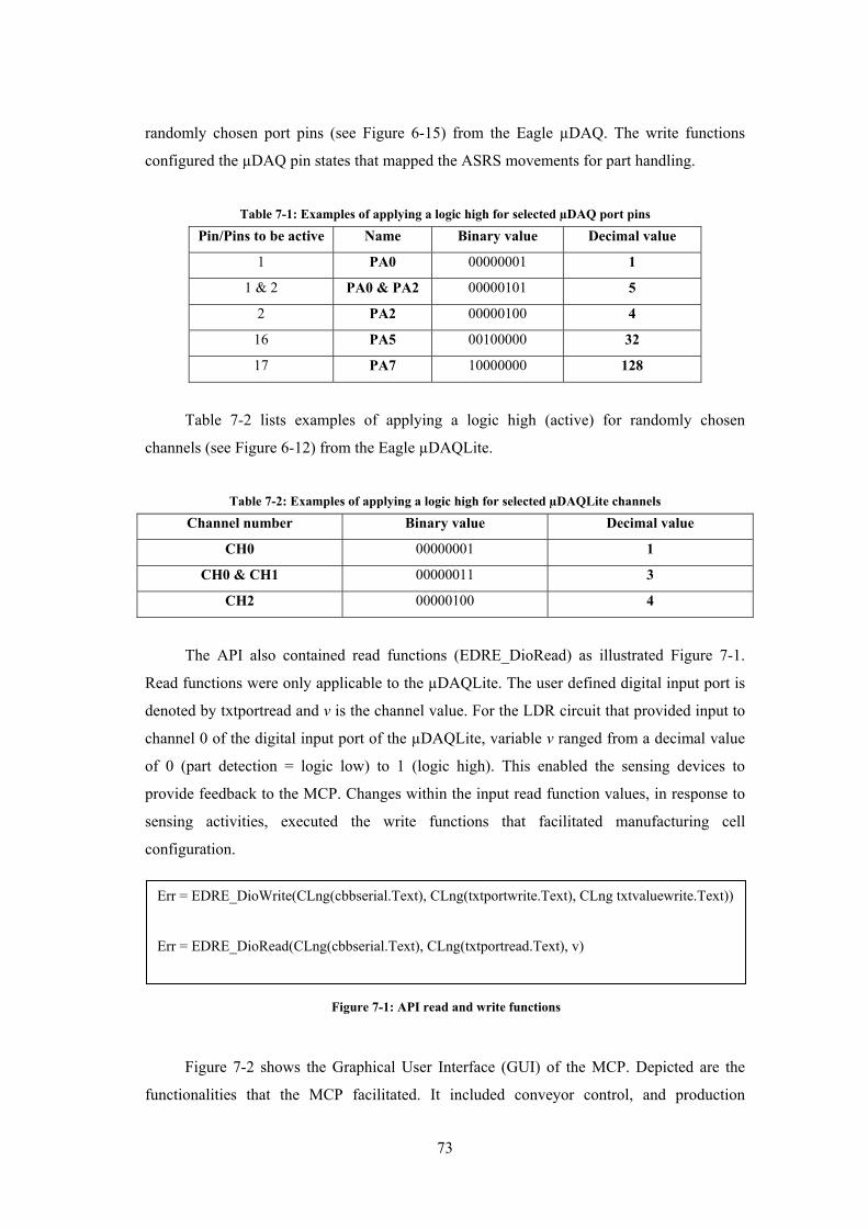
73

randomly chosen port pins (see Figure 6-15) from the Eagle µDAQ. The write functions

configured the µDAQ pin states that mapped the ASRS movements for part handling.

Table 7-1: Examples of applying a logic high for selected µDAQ port pins

Pin/Pins to be active Name Binary value Decimal value

1 PA0 00000001 1

1 & 2 PA0 & PA2 00000101 5

2 PA2 00000100 4

16 PA5 00100000 32

17 PA7 10000000 128

Table 7-2 lists examples of applying a logic high (active) for randomly chosen

channels (see Figure 6-12) from the Eagle µDAQLite.

Table 7-2: Examples of applying a logic high for selected µDAQLite channels

Channel number Binary value Decimal value

CH0 00000001 1

CH0 & CH1 00000011 3

CH2 00000100 4

The API also contained read functions (EDRE_DioRead) as illustrated Figure 7-1.

Read functions were only applicable to the µDAQLite. The user defined digital input port is

denoted by txtportread and v is the channel value. For the LDR circuit that provided input to

channel 0 of the digital input port of the µDAQLite, variable v ranged from a decimal value

of 0 (part detection = logic low) to 1 (logic high). This enabled the sensing devices to

provide feedback to the MCP. Changes within the input read function values, in response to

sensing activities, executed the write functions that facilitated manufacturing cell

configuration.

Figure 7-2 shows the Graphical User Interface (GUI) of the MCP. Depicted are the

functionalities that the MCP facilitated. It included conveyor control, and production

Err = EDRE_DioWrite(CLng(cbbserial.Text), CLng(txtportwrite.Text), CLng txtvaluewrite.Text))

Err = EDRE_DioRead(CLng(cbbserial.Text), CLng(txtportread.Text), v)

Figure 7-1: API read and write functions

74

execution and termination. The GUI also provided an input for customer order requirements

that included parts per order and due date (minutes). Upon execution, these input values were

computed by the MCP, and displayed priority coefficient values and order execution

arrangements as illustrated in Figure 7-3.

Figure 7-3: MCP with customer input values

Figure 7-2: MCP GUI developed with VB6

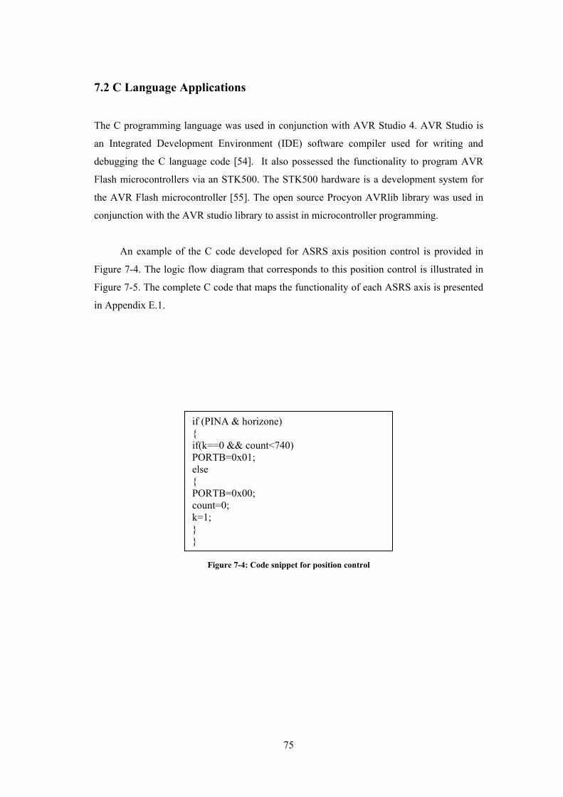
75

7.2 C Language Applications

The C programming language was used in conjunction with AVR Studio 4. AVR Studio is

an Integrated Development Environment (IDE) software compiler used for writing and

debugging the C language code [54]. It also possessed the functionality to program AVR

Flash microcontrollers via an STK500. The STK500 hardware is a development system for

the AVR Flash microcontroller [55]. The open source Procyon AVRlib library was used in

conjunction with the AVR studio library to assist in microcontroller programming.

An example of the C code developed for ASRS axis position control is provided in

Figure 7-4. The logic flow diagram that corresponds to this position control is illustrated in

Figure 7-5. The complete C code that maps the functionality of each ASRS axis is presented

in Appendix E.1.

if (PINA & horizone) { if(k==0 && count<740) PORTB=0x01; else { PORTB=0x00; count=0; k=1; } }

Figure 7-4: Code snippet for position control

76

7.3 Robotic Arm Teaching

The point to point teaching of the robotic arm in space was generated from utilising the

Fanuc programming language. A teach pendant, depicted in Figure 7-6 enabled the user to

manipulate and store the point to point positions of the robotic arm. The teach pendant

display screen provided an interface for user communication and selection of various

available functionalities. Prior to point to point programming, setting of the tool centre point

Figure 7-5: Logic diagram for ASRS position control

77

and user frames for calibration and vision processes were required [56]. The programmed

code with vision capabilities is shown in Appendix E.3. In collaboration with robotic arm

functionality, the Fanuc iRvision software facilitated additional robot flexibility.

7.3.1 iRvision Software

iRvision is a Fanuc incorporated vision package contained in the robot main controller.

Installation and user functionality of the vision software was done via a network cable that

linked the robot main controller to the HRCIM cell PC. The robot controller possessed an IP

address which was used to access the iRvision software from the Microsoft Internet Explorer

main frame as illustrated in Figure 7-7. The iRvision software enabled the user to perform

camera calibrations for precise part locating in collaboration with the robotic arm TCP.

Software related functionalities included part geometry teaching and customising the

bounded space for vision processing. The software GUI also provided a coordinated view of

the conveyor system that was in scope of the 2D camera as depicted in Figure 7-8.

Explanation of the diverse and sophisticated functionalities of the robotic arm with its

integrated vision capabilities is a broad area. Detailed illustrations are too extensive and were

not in scope of this research. Programming that proved viable to the required functionalities

Figure 7-6: Teach pendant

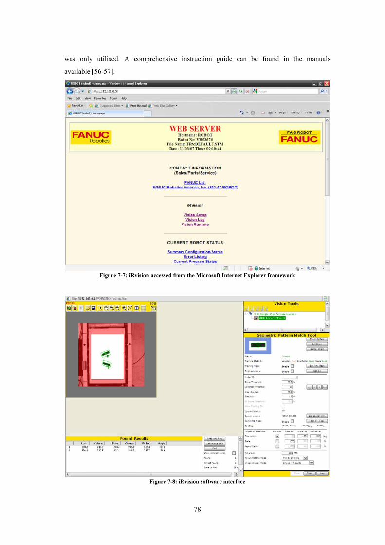
78

was only utilised. A comprehensive instruction guide can be found in the manuals

available [56-57].

Figure 7-8: iRvision software interface

Figure 7-7: iRvision accessed from the Microsoft Internet Explorer framework

79

7.4 Chapter Summary

This Chapter detailed software design and applications that customised HRCIM cell

behaviour. MCP design and programming of embedded applications were included.

Explanations for robotic arm teaching, with integrated software vision applications were also

listed. In combination with section 5-6, this chapter completes the fulfilment of the

mechatronic and intelligent agent design approach.

80

8. Testing and Results

Real time operational data was extracted from the HRCIM cell hardware. The majority of the

data was averaged from repeated tests. Averaged data comprised of part retrieval times, and

material handling speeds and times. In contrary, CNC part processing times were gathered

from a path simulator. Limitations within the research environment to encapsulate

coordinated hardware behaviour were inevitable. The averaged data was used to model a

software based simulation of the HRCIM cell.

Analysis of manufacturing events included algorithm based priority scheduling.

Hardware and part type processing results were also generated and analysed.

8.1 Algorithm Based Priority Scheduling

Software computed priority scheduling provided the structured retrieval of parts for

processing orders. With reference to Chapter 7.1, experiments which imitated authentic

customer input for scheduling production were facilitated. The experiments were based on

discrete events that involved frequently changing part types and quantities. This was in

contrast to the traditional systematic FIFO approach.

Four parts identified as A, B, C and D were randomly selected to represent custom

parts. These parts possessed different geometries that entailed robot material handling

reconfiguration (see Chapter 5.2.1). The parts also contained different CNC processing times

and machining requirements.

EdgeCam, an offline CNC path simulator software was used to compute the CNC part

processing times. Figure 8-1 shows an EdgeCam simulation for Part A. Part A corresponded

to the part library found in Figure 4-12. This approach was also generated for Part B, C and

D. Table 8-1 lists these part types and is represented by Pt. Ti indicates the time an order was

initiated and Td the time an order was due. Variables not mentioned from Table 8-1 are

defined in Chapter 7.1. A total of thirty five parts summed from column Pi were used to

perform the priority scheduling experiment. This data computed production scheduling based

on priority values Cpriority [58]. The computation was generated by using Equations 7.1

and 7.2. The graph depicted in Figure 8-2 [58] illustrates the prioritisation level for each

customer order.

81

Figure 8-1: EgdeCam part simulator

Figure 8-2: Priority values for each customer order [58]

Table 8-1: Customer order input values and processing times

Customer order

no. Pi Pt

PTp

(min)

Td

(Hours)

Ti

(Hours)

Tf = Td -Ti

(min)

Cpriority

value

1 10 A 16.090 14:00 8:00 360 2.237

2 5 B 8.513 13:00 8:20 280 6.578

3 5 C 13.807 15:30 10:00 330 4.78

4 15 D 8.79 15:30 9:00 390 2.958

82

The lowest priority coefficient (Cpriority) for the corresponding customer order was

processed first. In contrast, the customer order with the highest priority coefficient (Cpriority)

was processed last. Results from Figure 8-2 and Table 8-1 shows that customer order one

was processed first and last was customer order two [58].

8.2 Equipment Testing

8.2.1 Part Dependent Operations

Certain HRCIM cell equipment possessed discrete functionality due to frequently changing

part type demands. For specified part type demands, retrieval or material handling times

differed. Equipment that was subjected to these changes included the ASRS and robotic

arms.

8.2.1.1 ASRS Testing

ASRS testing included part retrieval times from different ASRS storage points. As depicted

in Figure 4-9 the storage location points for part A, B, C and D are shown. Table 8-2 lists the

computed retrieval times for each part type. The tests results used to attain these retrieval

times is tabulated in Appendix D.2. The ASRS crane was initially placed at the reference

point. Retrieval time of the first part was therefore taken from the reference point. After

unloading the first part, the crane was situated at the ASRS unloading zone. When retrieval

of parts to follow was initiated, the time taken to return to the reference point for position

calibration was also taken into account.

Table 8-2: ASRS retrieval time per part type

Part

Average retrieval time, crane

movement initiated from

reference point (seconds)

Average retrieval time, crane

movement initiated from

unloading point (seconds)

A 15.85 18.3

B 17.98 20.43

C 18.47 20.92

D 20.51 22.96

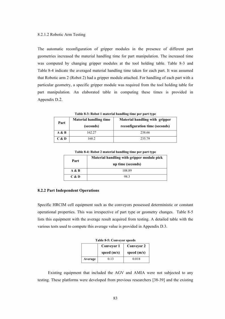
83

8.2.1.2 Robotic Arm Testing

The automatic reconfiguration of gripper modules in the presence of different part

geometries increased the material handling time for part manipulation. The increased time

was computed by changing gripper modules at the tool holding table. Table 8-3 and

Table 8-4 indicate the averaged material handling time taken for each part. It was assumed

that Robotic arm 2 (Robot 2) had a gripper module attached. For handling of each part with a

particular geometry, a specific gripper module was required from the tool holding table for

part manipulation. An elaborated table in computing these times is provided in

Appendix D.2.

Table 8-3: Robot 1 material handling time per part type

Part Material handling time

(seconds)

Material handling with gripper

reconfiguration time (seconds)

A & B 162.27 238.66

C & D 160.2 235.79

Table 8-4: Robot 2 material handling time per part type

Part Material handling with gripper module pick

up time (seconds)

A & B 108.89

C & D 98.3

8.2.2 Part Independent Operations

Specific HRCIM cell equipment such as the conveyors possessed deterministic or constant

operational properties. This was irrespective of part type or geometry changes. Table 8-5

lists this equipment with the average result acquired from testing. A detailed table with the

various tests used to compute this average value is provided in Appendix D.3.

Table 8-5: Conveyor speeds

Conveyor 1

speed (m/s)

Conveyor 2

speed (m/s)

Average 0.13 0.018

Existing equipment that included the AGV and AMIA were not subjected to any

testing. These platforms were developed from previous researchers [38-39] and the existing

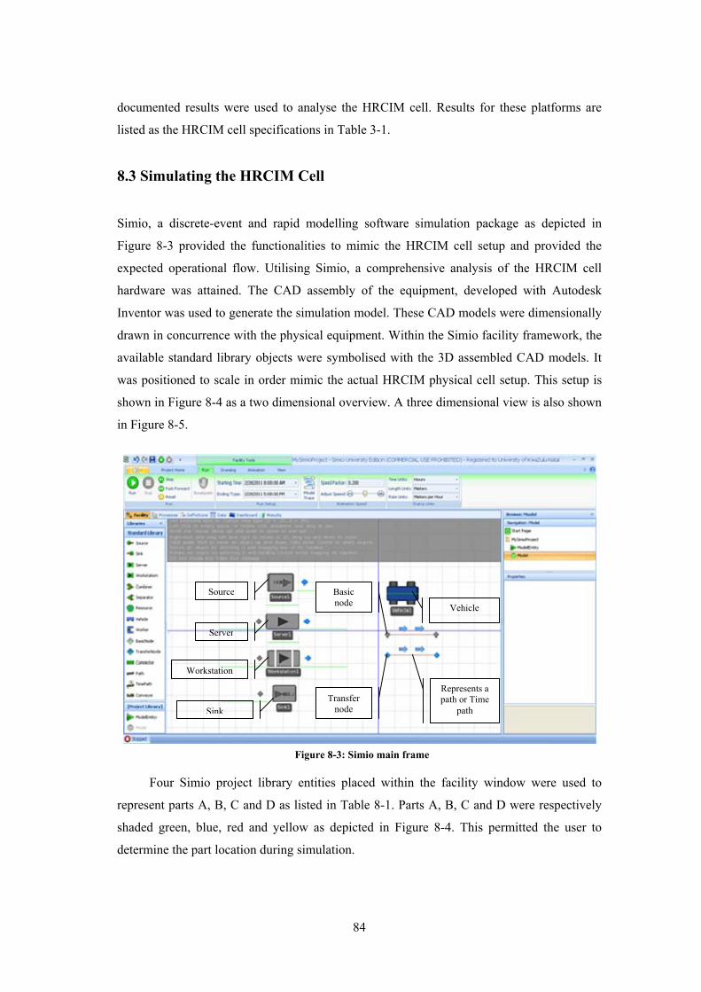
84

documented results were used to analyse the HRCIM cell. Results for these platforms are

listed as the HRCIM cell specifications in Table 3-1.

8.3 Simulating the HRCIM Cell

Simio, a discrete-event and rapid modelling software simulation package as depicted in

Figure 8-3 provided the functionalities to mimic the HRCIM cell setup and provided the

expected operational flow. Utilising Simio, a comprehensive analysis of the HRCIM cell

hardware was attained. The CAD assembly of the equipment, developed with Autodesk

Inventor was used to generate the simulation model. These CAD models were dimensionally

drawn in concurrence with the physical equipment. Within the Simio facility framework, the

available standard library objects were symbolised with the 3D assembled CAD models. It

was positioned to scale in order mimic the actual HRCIM physical cell setup. This setup is

shown in Figure 8-4 as a two dimensional overview. A three dimensional view is also shown

in Figure 8-5.

Four Simio project library entities placed within the facility window were used to

represent parts A, B, C and D as listed in Table 8-1. Parts A, B, C and D were respectively

shaded green, blue, red and yellow as depicted in Figure 8-4. This permitted the user to

determine the part location during simulation.

Figure 8-3: Simio main frame

Transfer node

Basic node

Represents a path or Time

path

Server

Source

Workstation

Sink

Vehicle

85

The available standard library contained various objects that were use to model the

HRCIM cell. Figure 8-3 depicts these objects and Table 8-6 explains the functionality for

each.

Table 8-6: Simio object definition and hardware represented

OBJECT Hardware symbolised Functionality

Basic node - Used for generating links or paths

Transfer node

- Generates links or parts - Provides transport logic and part

destination options for the AGV and robotic arms

Path Conveyor 1 & 2

- Defines a pathway between two nodes

- The travel time is determined from the path length and the traveller's (AGV or part) speed

Time path Robot 1 and Robot 2 material handling time

- Used to define a pathway between nodes with a user-specified travel time

Source - Generates parts (entities) to enter

the model

Server ASRS - Used to model a capacitated process

Vehicle AGV, Robot 1 & 2 - Transport parts (entities) between

nodes

Workstation CNC machine and the AMIA

- Provides operational activities that include setup and processing times

Sink - Destroys parts that have finished

processing in the model

Figure 8-4: Simio 2D overview of the HRCIM cell

86

Figure 8-5: Simio 3D overview of the HRCIM cell

The test results in sections 8.1 and 8.2 and the relevant specifications given in

Table 3-1 were used to apply operational parameters for the simulated HRCIM cell and its

equipment.

A time framework for the simulation was also necessary. The simulation was set for

nine hours to complete all the customer orders. Within the Simio simulation setup, the start

time was set at 8:00 am and ended at 5:00 pm. User defined simulation speeds were also

optional. A complete simulation was achieved within seconds or minutes depending on the

simulation speed. After a complete simulation a detailed spreadsheet was provided that

elaborated on each object within the HRCIM cell. Animated graphs and pie charts were also

provided. Pie charts produced results that were instantaneous with time and were only

meaningful during a simulation. It was therefore not necessary to implement it for every

equipment or part analysis to follow.

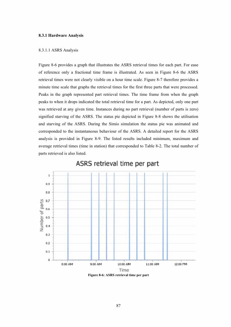
87

8.3.1 Hardware Analysis

8.3.1.1 ASRS Analysis

Figure 8-6 provides a graph that illustrates the ASRS retrieval times for each part. For ease

of reference only a fractional time frame is illustrated. As seen in Figure 8-6 the ASRS

retrieval times were not clearly visible on a hour time scale. Figure 8-7 therefore provides a

minute time scale that graphs the retrieval times for the first three parts that were processed.

Peaks in the graph represented part retrieval times. The time frame from when the graph

peaks to when it drops indicated the total retrieval time for a part. As depicted, only one part

was retrieved at any given time. Instances during no part retrieval (number of parts is zero)

signified starving of the ASRS. The status pie depicted in Figure 8-8 shows the utilisation

and starving of the ASRS. During the Simio simulation the status pie was animated and

corresponded to the instantaneous behaviour of the ASRS. A detailed report for the ASRS

analysis is provided in Figure 8-9. The listed results included minimum, maximum and

average retrieval times (time in station) that corresponded to Table 8-2. The total number of

parts retrieved is also listed.

Figure 8-6: ASRS retrieval time per part

88

Figure 8-8: Pie chart indicating ASRS resource state

Figure 8-7: ASRS retrieval time for first three parts

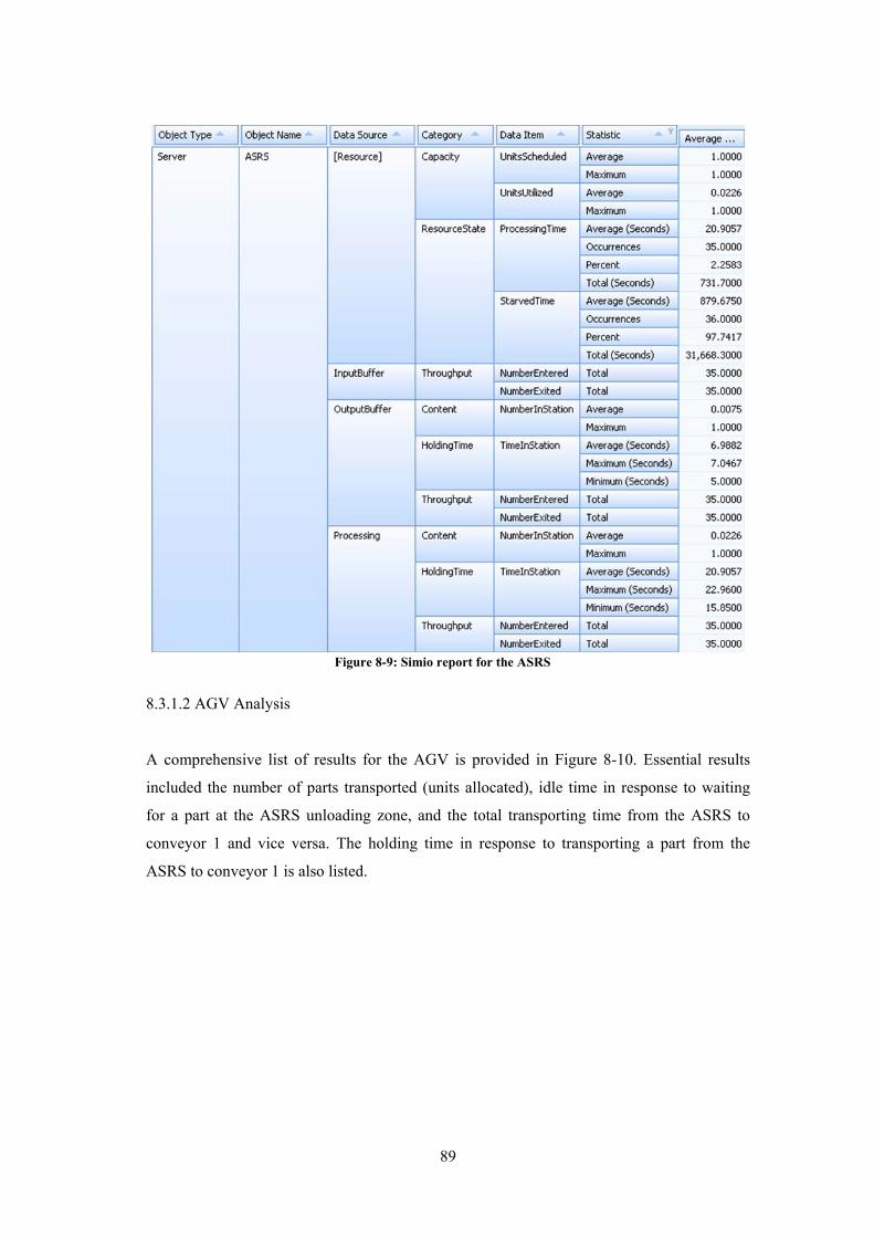
89

8.3.1.2 AGV Analysis

A comprehensive list of results for the AGV is provided in Figure 8-10. Essential results

included the number of parts transported (units allocated), idle time in response to waiting

for a part at the ASRS unloading zone, and the total transporting time from the ASRS to

conveyor 1 and vice versa. The holding time in response to transporting a part from the

ASRS to conveyor 1 is also listed.

Figure 8-9: Simio report for the ASRS

90

8.3.1.3 Conveyor Analysis for Processing Cell 1

A transfer node from the Simio standard library was placed at the vision processing platform

of the conveyor. Due to more user defined functionalities as compared to the limitations of

the physical setup, this transfer node served as a buffer. Only one part could be present at

this node for CNC processing at any given time. When a part left the simulated CNC

machine after being processed, robot manipulation for part retrieval from this transfer node

or vision processing platform was initiated. These retrieval times were unattainable within

the physical setup.

The graph shown in Figure 8-11 represents the buffering time of parts and the time

upon which robot part manipulation takes place. Steps in the graph indicate the time robot

part manipulation was initiated for CNC processing. To provide a legible evaluation, the

graph illustrated in Figure 8-12 is taken over a reduced time frame and indicates the

buffering time (horizontal line) for each part. Numerical results indicating the total time

conveyor 1 accommodated part flow (flow time) is specified in Figure 8-13. The number of

parts entered and exited (throughput) at conveyor 1 is also provided.

Figure 8-10: Simio report for the AGV

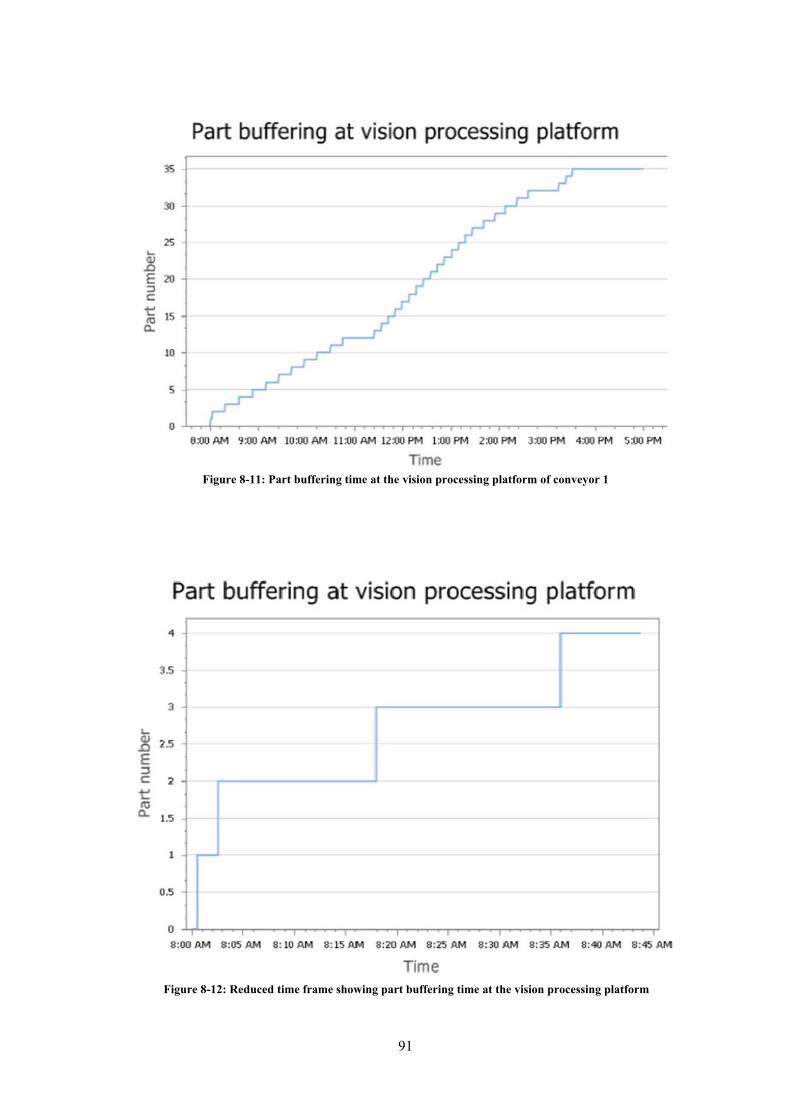
91

Figure 8-12: Reduced time frame showing part buffering time at the vision processing platform

Figure 8-11: Part buffering time at the vision processing platform of conveyor 1

92

8.3.1.4 CNC Machine Analysis

The CNC machine was subjected to changeover of its setup for machining specified parts

types. Table D.6 in Appendix D.2 provides a matrix that illustrates the changeover time

required for processing between different part types. An assumed 30 minute machine

changeover time was selected. This was based on knowledge acquired from qualified

personnel. As tabulated, changeover or setup times between similar part geometries were

neglected. To be explicit, Parts A and B possessed similar geometries. This same property

applied to Parts C and D. The symbolised part geometry was elaborated in Chapter 4.4.1.

The graph presented in Figure 8-14 maps the time a part enters (number entered) and

exits (number exited) the CNC machine. A magnified view of Figure 8-14 that is taken over

a condensed time frame is presented in Figure 8-15. The total processing time for a part is

represented from when it enters to when it exits.

An in-depth CNC machine analysis is also prescribed in Figure 8-16. Highlighted

manufacturing events recorded included parts allocated, processing time, setup time, starved

time and entry queue data. Starved time is the accumulated time during which no parts are

being processed. Entry queue data included the CNC machine input buffer times (time

waiting) for which parts queued for processing.

Figure 8-13: Simio report for Conveyor 1

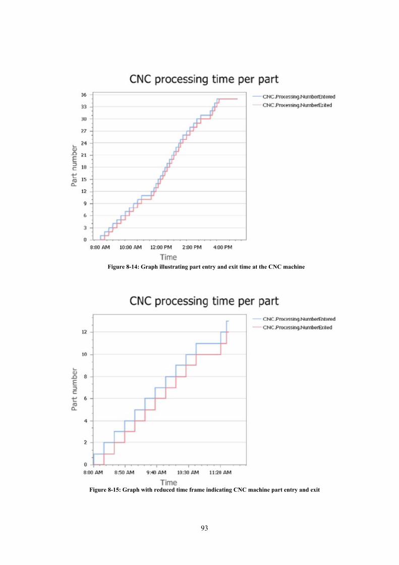
93

Figure 8-15: Graph with reduced time frame indicating CNC machine part entry and exit

Figure 8-14: Graph illustrating part entry and exit time at the CNC machine

94

Figure 8-16: Simio report for the CNC workstation

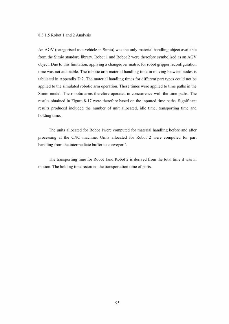
95

8.3.1.5 Robot 1 and 2 Analysis

An AGV (categorised as a vehicle in Simio) was the only material handling object available

from the Simio standard library. Robot 1 and Robot 2 were therefore symbolised as an AGV

object. Due to this limitation, applying a changeover matrix for robot gripper reconfiguration

time was not attainable. The robotic arm material handling time in moving between nodes is

tabulated in Appendix D.2. The material handling times for different part types could not be

applied to the simulated robotic arm operation. These times were applied to time paths in the

Simio model. The robotic arms therefore operated in concurrence with the time paths. The

results obtained in Figure 8-17 were therefore based on the inputted time paths. Significant

results produced included the number of unit allocated, idle time, transporting time and

holding time.

The units allocated for Robot 1were computed for material handling before and after

processing at the CNC machine. Units allocated for Robot 2 were computed for part

handling from the intermediate buffer to conveyor 2.

The transporting time for Robot 1and Robot 2 is derived from the total time it was in

motion. The holding time recorded the transportation time of parts.

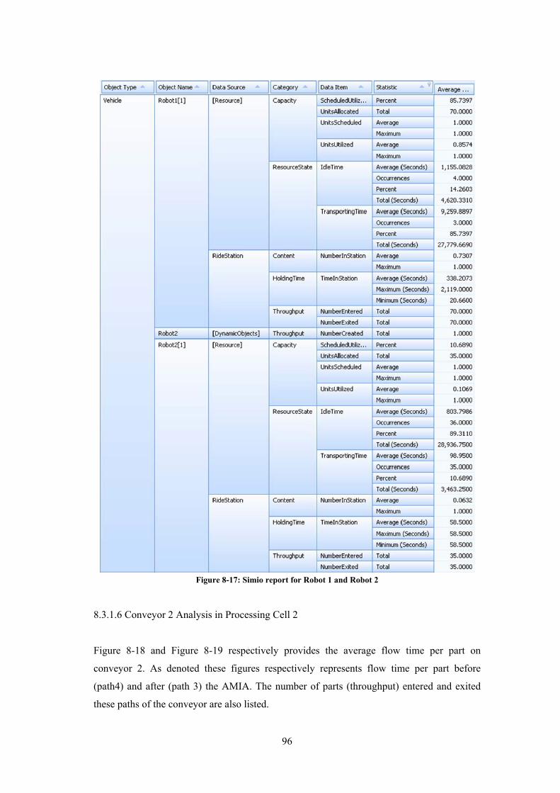
96

8.3.1.6 Conveyor 2 Analysis in Processing Cell 2

Figure 8-18 and Figure 8-19 respectively provides the average flow time per part on

conveyor 2. As denoted these figures respectively represents flow time per part before

(path4) and after (path 3) the AMIA. The number of parts (throughput) entered and exited

these paths of the conveyor are also listed.

Figure 8-17: Simio report for Robot 1 and Robot 2

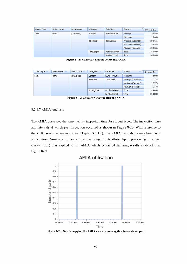
97

8.3.1.7 AMIA Analysis

The AMIA possessed the same quality inspection time for all part types. The inspection time

and intervals at which part inspection occurred is shown in Figure 8-20. With reference to

the CNC machine analysis (see Chapter 8.3.1.4), the AMIA was also symbolised as a

workstation. Similarly the same manufacturing events (throughput, processing time and

starved time) was applied to the AMIA which generated differing results as denoted in

Figure 8-21.

Figure 8-20: Graph mapping the AMIA vision processing time intervals per part

Figure 8-19: Conveyor analysis after the AMIA

Figure 8-18: Conveyor analysis before the AMIA

98

8.3.2 Part Analysis

Determining the total time from when a part has entered to when it exits the manufacturing

cell is an imperative factor for manufacturers. It enables a manufacturer to predetermine

product cycle times and arrange customer orders accordingly. This was facilitated by

utilising the Simio source and sink objects.

The source object created parts (entities) based on CNC input buffer status. In

response each created part possessed an initial retrieval time. Part flow time between the

source and ASRS (server) was neglected by configuring the Simio based path options. The

time at which each part exited the manufacturing cell was generated from the sink object.

The sink object also registered a finished product.

The graph generated in Figure 8-22 indicates the initial retrieval time for parts. The

graph contains initial retrieval times for part types A, B, C and D. The order in which parts

are retrieved corresponds to the priority values indicated in Table 8-1 and Figure 8-2. Steps

in the graph signify a call for part retrieval.

Figure 8-21: Simio generated results for the AMIA

99

Individual magnified graphs for each part type relating to initial retrieval time is

provided in Figure 8-23 to Figure 8-26. The figures presented, follows the arrangement in

which parts were processed. Extended time lengths between steps in each graph indicate that

the input CNC buffer has reached its maximum allowable capacity which prevents further

initiation for part retrieval.

Figure 8-22: Graph indicating the initial retrieval time for all part types

Figure 8-23: Graph indicating the initial retrieval time for part type A

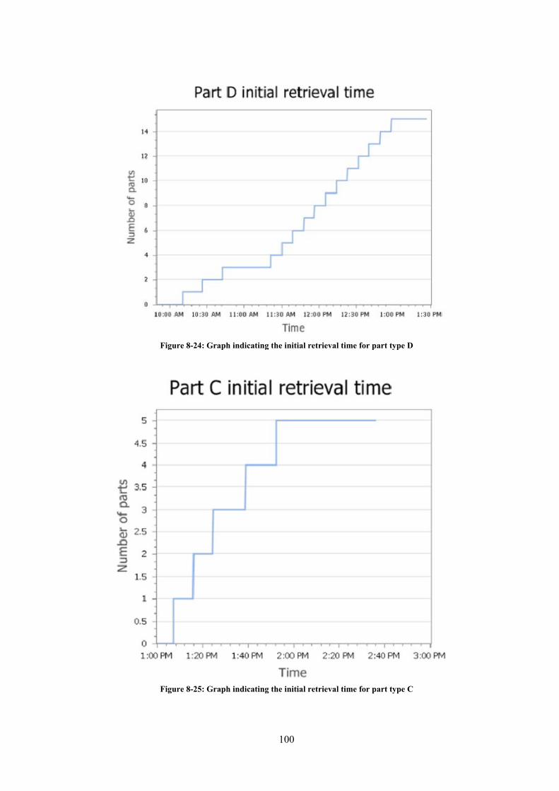
100

Figure 8-24: Graph indicating the initial retrieval time for part type D

Figure 8-25: Graph indicating the initial retrieval time for part type C

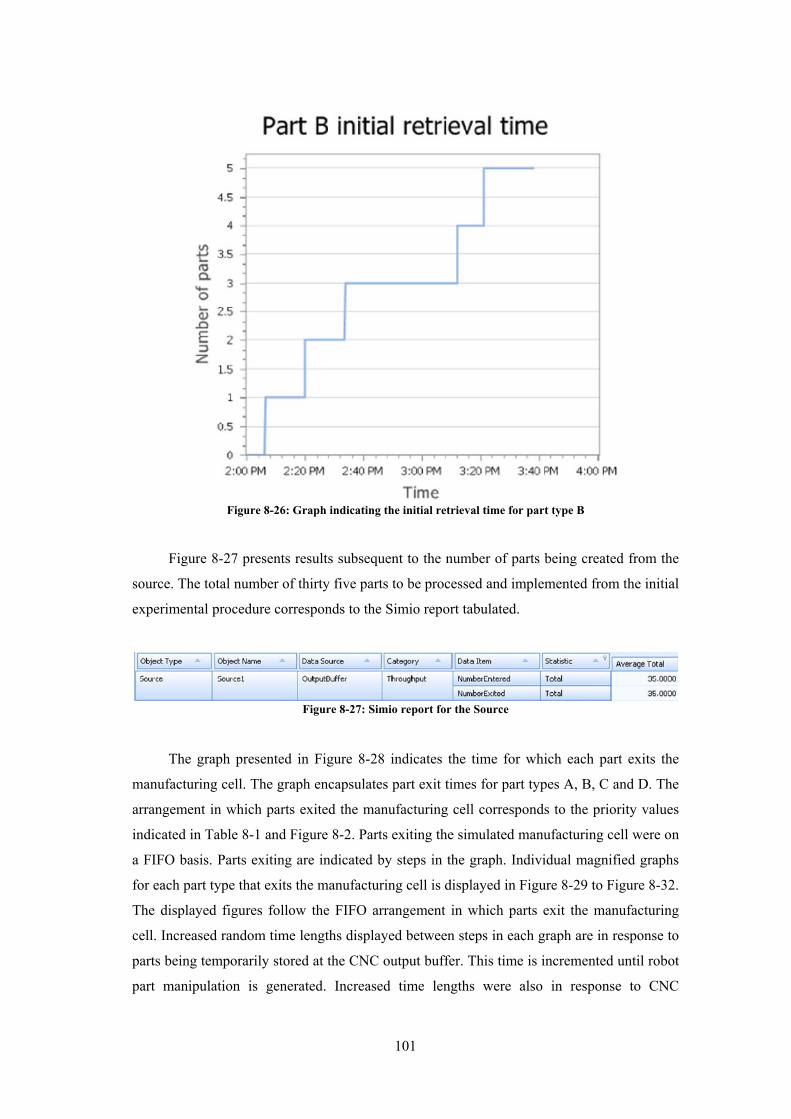
101

Figure 8-27 presents results subsequent to the number of parts being created from the

source. The total number of thirty five parts to be processed and implemented from the initial

experimental procedure corresponds to the Simio report tabulated.

The graph presented in Figure 8-28 indicates the time for which each part exits the

manufacturing cell. The graph encapsulates part exit times for part types A, B, C and D. The

arrangement in which parts exited the manufacturing cell corresponds to the priority values

indicated in Table 8-1 and Figure 8-2. Parts exiting the simulated manufacturing cell were on

a FIFO basis. Parts exiting are indicated by steps in the graph. Individual magnified graphs

for each part type that exits the manufacturing cell is displayed in Figure 8-29 to Figure 8-32.

The displayed figures follow the FIFO arrangement in which parts exit the manufacturing

cell. Increased random time lengths displayed between steps in each graph are in response to

parts being temporarily stored at the CNC output buffer. This time is incremented until robot

part manipulation is generated. Increased time lengths were also in response to CNC

Figure 8-27: Simio report for the Source

Figure 8-26: Graph indicating the initial retrieval time for part type B

102

Figure 8-29: Time for which part type A exits the manufacturing cell

changeover times. This condition temporarily provided no CNC processed parts to the CNC

output buffer and hence generated an expanded time frame between exiting parts at the sink.

Figure 8-28: Graph indicating the time for which parts exit the HRCIM cell

103

Figure 8-30: Time for which part type D exits the manufacturing cell

Figure 8-31: Time for which part type C exits the manufacturing cell

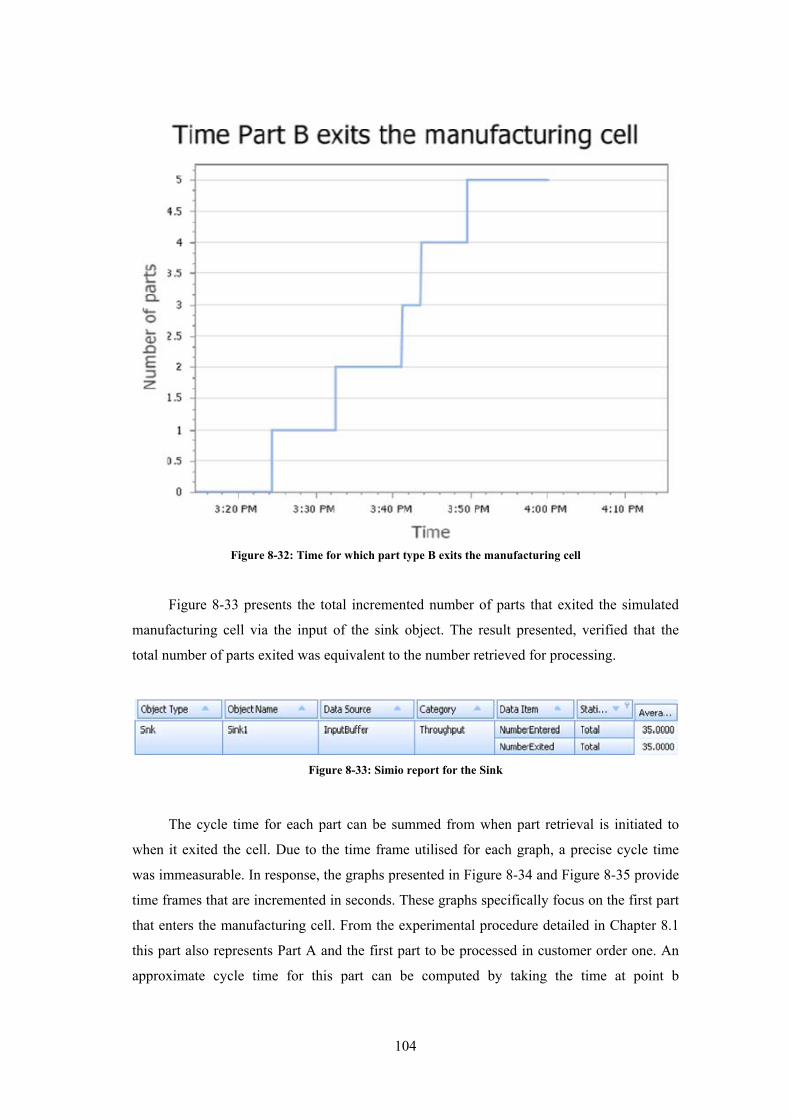
104

Figure 8-33 presents the total incremented number of parts that exited the simulated

manufacturing cell via the input of the sink object. The result presented, verified that the

total number of parts exited was equivalent to the number retrieved for processing.

The cycle time for each part can be summed from when part retrieval is initiated to

when it exited the cell. Due to the time frame utilised for each graph, a precise cycle time

was immeasurable. In response, the graphs presented in Figure 8-34 and Figure 8-35 provide

time frames that are incremented in seconds. These graphs specifically focus on the first part

that enters the manufacturing cell. From the experimental procedure detailed in Chapter 8.1

this part also represents Part A and the first part to be processed in customer order one. An

approximate cycle time for this part can be computed by taking the time at point b

Figure 8-33: Simio report for the Sink

Figure 8-32: Time for which part type B exits the manufacturing cell

105

(see Figure 8-35) and subtracting the time at point a (see Figure 8-34). Cycle times for the

parts to follow can be approximated by utilising this same concept.

Figure 8-35: Time for which the first part of customer one exits the manufacturing cell

b

Figure 8-34: Time for which the first part of customer order one is initiated for retrieval

a

106

Figure 8-36 provides significant results that incorporate the average, minimum and

maximum time each part type was encapsulated within the HRCIM cell. The number of parts

processed for each part type (customer order) is also presented.

8.4 Chapter Summary

This chapter outlined the procedures for which tests were facilitated. Results were generated

from priority based scheduling and software executed manufacturing simulation. The

simulated HRCIM cell results were disintegrated at a machine level. Simulated results for

each part type are also presented. The simulated results contained graphs and detailed reports

that facilitated research analysis.

Figure 8-36: Simio report for part types produced

107

9. Discussion

9.1 Performance Measures Prior to HRCIM Cell Simulation

Given the required time frame, research to provide a comprehensive analysis of the HRCIM

was unattainable. Measured HRCIM cell equipment performance values subsequent to

successful calculated design or operational constraints were used to model the simulated

manufacturing cell. These constraints were in relation to mechanical, electronic and software

based functionality. Specifications provided in Chapter 3.3 were also used to parameterise

the simulated HRCIM cell behaviour.

9.1.1 Mechanical Constraints

The robotic arm vision camera support required a balanced and weighted mechanical

structure due to its sensitivity. Fillet weld A and B, depicted in Figure 5-2 required a

theoretical minimum weld height of 0.033 mm and 0.0125 mm respectively. From physical

measuring procedures, the assembled camera support possessed a weld height which was

within limits. The deflection of the camera from the cantilevered end of the camera support

was computed to be 0.64 mm. Reviewed image processing experiments in response to this

theoretical camera deflection did not render incorrect part locations.

Bolted gripper module interfaces were subjected to withstand the gripper and interface

weight acting against it. The maximum external force required for interface joint separation

was extensively within limits and supported the respective gripper module weights. The total

joint separation force that supported the specified weights is tabulated in Table 5-7.

9.1.2 Electronic Constraints

The response time for the LDR to facilitate a logic change occurred in milliseconds

(see Figure 6-2). This responsive feedback enabled synchronised and coordinated material

handling system behaviour that facilitated the seamless measuring of part handling times.

108

9.1.3 Software Constraints

Distributed software control mapped the ASRS part retrieval paths and in response part

retrieval times were summed for simulation purposes.

9.2 Measured Values to Parameterise the HRCIM Cell Simulation

The simulation parameters were inserted with actual laboratory based HRCIM cell measured

values. Differing operational parameters between the simulated and physical cell were

therefore neglected. The simulated cell was assumed to have equivalent operational

characteristics in relation to the physical HRCIM cell. Specifications and measured values

utilised are provided in Chapter 3.3, 8.1 and 8.2.

9.3 Simulated Results

Simio generated results facilitated research analysis of the HRCIM cell. Graphs and reports

available in Chapter 8.3, provided part buffering, product cycle times and machine

changeover analysis that were in response to introducing frequently changing part

geometries.

The initial simulated HRCIM cell consisted of bottle necks at the CNC machine input

buffer. This was due to the continuous retrieval of parts from the ASRS. By adjusting the

logic for part retrieval from the ASRS and the vision platform at conveyor 1, a systematic

flow of parts was achieved. A processed part at the CNC machine output buffer resulted in

part retrieval from the vision platform of conveyor 1. The vision platform of conveyor 1 was

modelled to always possess a single part, if available from the ASRS. The simulated robotic

arm, subsequent to visual capture of a part, loaded the CNC machine with the captured part.

The simulated model was user restricted to occupy a single part at the CNC machine input

buffer. The graphs displayed in Chapter 8.3 provided research to study part behaviour and

the discrete behaviour of part flow. WIP for each part was mapped. The effects of machine

reconfiguration, required to process different part geometries were examined (section 8.3.2).

This machine reconfiguration (changeover) temporarily inhibited further part retrieval from

buffers or material handling equipment. Results provided for part analysis, allowed for

detailed part buffering and cycle time investigations that were generated during machine

reconfiguration. This final simulated HRCIM cell design provided a systematic flow of parts.

109

In conclusion, seamless equipment operations were generated between computer integrated

and RMS technology. Computer integrated technology represented part scheduling of

irregular part types or geometries. RMS technology represented reconfiguration of the

robotic arm end effector that facilitated manipulation of different part geometries.

9.4 Reviewed HRCIM Cell Objectives

The flexibility and reconfigurability experienced from the physical environment to perform

material handling for discrete part geometry flow (represented MC) fulfilled related research

motives listed in Chapter 1.3. From an industry perspective this computer controlled

reconfigurable cell introduced an intelligent and automated approach for conducting MC.

The developed cell also verified resource specifications and capabilities. The prearranged

and user established resources met the requirements to facilitate the project objectives.

9.5 HRCIM in Comparison to RMS and FMS

Detailed HRCIM cost analyses was beyond the scope of this research. Research undertaken

provided reasons to evaluate cost in comparison to RMS and FMS. The developed cell is

measured to cost more in relation to RMSs. Reasons include the high cost of CNC

equipment and the addition of complete computer controlled automation for RMS

equipment. In relation to FMS, HRCIM technology is measured to cost less. Reasons

incorporate the inclusion of cheaper but yet less flexible CNC equipment into the HRCIM

cell. FMS in response to its high cost possesses expensive CNC equipment that contains

excessive functionalities which are not utilised. The HRCIM cell architecture therefore

possessed specific FMS and RMS functionalities that were neither excessive nor inadequate

in its capabilities.

Part production in a RMS is limited to part families. In a FMS, customised or a variety

of parts are manufactured due to its excessive functionalities. The researched HRCIM cell in

comparison to RMS and FMS strategies facilitated the manufacture of mass customised

parts. This approach limited the number of custom products manufactured. Customer

demand for custom products was therefore limited. Utilising this approach reduced cell

changeover time and computer aided manufacturing processes required for new custom

parts. A fixed library of custom parts therefore eliminated preparation time. This seamless

110

process that facilitated discrete events enabled custom parts to be manufactured at a mass

rate.

From a machine structure perspective, RMS and FMS possess an adjustable and fixed

architecture respectively (see Table 2-1). In contrast, the HRCIM cell contained both

adjustable and fixed characteristics, adopted from RMS and FMS respectively. The HRCIM

cell adjusted its material handling capabilities during discrete part geometry flow and

possessed a fixed architecture for part processing events.

System structure as tabulated in Table 2-1 is adjustable for both RMS and FMS. This

is driven by the manufacture of specific parts. The HRCIM cell was developed from these

strategies and in response also possessed this adjustable system or cell structure. This

adjustable functionality provided augmented flexibility for cell adaptation. RMS and FMS

adjustability is dependent on part families and part variety respectively. In contrast, HRCIM

cell adaptability was based on the manufacture of custom parts (see Figure 4-12) at near

mass production.

System flexibility for RMS is customised. Its flexibility is built around the

manufacture of a particular part family that requires processing. FMS in contrast possesses

general flexibility which is not designed around a specific part to be manufactured

(see Table 2-1). The developed HRCIM cell in relation to RMS was designed to consist of

customised flexibility. The measured custom flexibility required by the HRCIM cell was in

response to the manufacture of mass custom parts that were bounded in its variety.

The HRCIM cell in contrast to RMSs and FMSs (see Table 2-1) was similarly

measured to be scalable in its architecture. In the event of expanding production capacity,

addition of CNC or RMS equipment can be further integrated into the cell. Computer

controlled techniques (MCP) allows for formulating priority based scheduling for an

increased number of parts per customer order. The introduction of new custom parts that

concurrently increases the bounds for custom part variety can also be accommodated from

the MCP.

111

9.6 Observed HRCIM Cell Restrictions and Complications

9.6.1 Accuracy and Repeatability

Robot picking and placing of gripper modules from the tool holding table, required precise

accuracy and repeatability. In response to repeated pick and place events the robotic arm did

render slight offset values from the initial programmed pick and place points. The maximum

offset between the quick-change head and the quick-change adaptor prior to locking is

presented Table 5-2. To initiate correct pick and place points subsequent to exceeding the

maximum offset values, reprogramming of the robot pick and place points was facilitated.

ASRS crane positioning for pallet retrieval rendered errors associated with accuracy.

ASRS position control was in response to encoder incremented values. Repeated ASRS

movements from the reference point (see Figure 4-8) to the specified storage points

(see Figure 4-9) randomly rendered inaccurate crane positioning with reference to the storage

centre point. Performance measuring values were only extracted until the ASRS crane was in

line with the specified storage point.

9.6.2 Robotic Vision Calibration

Restrictions within the research environment prevented the permanent fixture of the vision

camera. The weighted camera support developed did reliably provide correct image

processing results for robot part pick and place operations. Slight environment disturbances

on the contrary did deviate camera position, which rendered incorrect robot end effector

positioning for part pick and place operations. Random manual calibration of the robot

vision system was therefore necessary to eliminate offset errors and provide the correct

calibrated points in space.

9.6.3 Limitations within RMS Technology

RMS technology to date, are yet to be further enhanced and be optimistically utilised in

manufacturing industries. Current RMS developed platforms in the research environment

were not robust mechanically and in their control. This included a modular tool-changing

unit and a five axis CNC drilling machine (see Figure 2-5). These platforms were limited to

research based testing and did not possess the sophisticated control architecture to operate in

112

the HRCIM cell. In response, RMS technology for the HRCIM was limited. The Fanuc

robotic arm with reconfigurable gripper (tool) changing modules therefore represented RMS

based technology in the HRCIM cell.

9.6.4 Research Assumptions

The high cost of state-of-the-art equipment to provide a fully functional physical HRCIM

cell was inevitable. Measured performance values were extracted from research developed

and refurbished equipment. These values were used as parameters in the simulated HRCIM

cell. It was assumed that objects (HRCIM cell equipment) in the simulated cell performed

approximately to that of the physical equipment.

9.6.5 Restrictions within the HRCIM Cell Simulation

The Simio software did not provide simulation flexibility for robotic arm gripper module

selection. The robotic arm was also assumed to be a vehicle object. Changeover matrix

developed within the Simio framework enabled reconfiguration for specific objects

(workstation). Applying a changeover matrix to the simulated robotic arm was inevitable.

Difference in material handling and gripper reconfiguration times between part handling

were therefore represented as load and unload times. The load and unload times were used to

customise the robotic arms travel logic for each part type.

9.7 Chapter Summary

This chapter discusses relevant design results used to support and generate specific cell

functionalities, and equipment performance measures. It examines simulated manufacturing

cell results in response to these measured performances. Research objectives gained, and a

comparative analysis in relation to RMS and FMS is presented. Highlighted research

restrictions and complications are also detailed.

113

10. Conclusion

Today’s customer driven market for mass customised parts has uplifted the technological

requirements for manufacturing industries. Manufacturing industries are still not capable to

produce mass customised parts timeously and cost effectively. This deficiency has induced

research in search of an innovative approach to efficiently produce mass customised parts.

This innovative approach facilitated the development of a HRCIM cell. The HRCIM cell

concurrently operated from RMS and CIM (includes FMS) characteristics. The researched

HRCIM cell behaviour was analysed in response to frequently changing part geometries that

represented custom parts.

The HRCIM cell in contrast to RMS and CIM (includes FMS) contained sufficient

reconfigurable and flexible characteristics to generate mass customised parts. It did not lack

nor was it excessive in its characteristics. The characteristics were mapped according to the

requirements needed to produce the custom parts available in the product or part library. This

defined an approach that bounded the required characteristics and in reply reduced cost.

The HRCIM cell architecture consisted of existing and new equipment that originated

from a device to machine level. The cell operated concurrently with integrated mechanical,

electronic and software functionality. Highlighted mechanical functionality consisted of a

reconfigurable robotic arm end effector that enabled material handling for specific part

geometries. This RMS characteristic was generated automatically subsequent to electronic

and software generated events.

HRCIM cell integration and control was generated by utilising electronic control

devices. It facilitated cell coordination and synchronisation between equipment. Highlighted

electronic control operations that facilitated mechanical actuation were in conjunction with

software related manufacturing scheduling activities. This provided the seamless cell

functionality in response to discrete part flow associated with MC.

Highlighted software functionalities that assisted MC included part geometry teaching

and algorithm based priority scheduling. Robot integrated vision processing software

facilitated part geometry teaching. This defined a unique pattern for a particular custom part.

This unique pattern was mapped to a specific gripper module during robot point to point and

vision programming. Priority based scheduling was independent to the vision process. It

114

enabled part retrieval for discrete customer orders. Discrete customer behaviour was in

response to varying parameters that included parts per order and due date.

Research limitations restricted actual HRCIM cell part processing. Square and circular

components represented the parts to be manufactured. This flow of irregular part geometries

symbolised custom part flow and was used to analyse HRCIM cell behaviour in response to

frequently changing part geometry definitions. Some HRCIM cell equipment was obsolete in

their functionality. This proposed incomplete or inefficient coordination between the

HRCIM cell equipment.

Key problematic areas during HRCIM cell development aroused from the inability to

provide a fully functional physical manufacturing cell. The simulated cell itself was

restricted in its functionality for robot reconfiguration in response to discrete part handling.

The limited functionality, generated by the physical cell setup however did provide sufficient

evidence in demonstrating how reconfigurable platforms operate in computer integrated

manufacturing cells. Highlighted functionalities were in response to effective robot end

effector configuration for manipulating discrete part geometry flow.

Project objectives that were fulfilled include the following:

The HRCIM cell did facilitate the discrete processing for different part types

which represented MC.

Material handling of different part types with frequently changing geometries was

accomplished.

The overall manufacturing cell possessed adequate flexibility and

reconfigurability to feasibly manufacture the custom parts offered.

These fulfilled objectives verified cell specifications that were in response to

hardware and software operations.

Prospective enhancements in RMS can generate future research for the HRCIM cell.

RMS platforms with improved design and control can be used to further analyse

reconfigurable operations in a computer integrated cell. Developing the cell with modern

manufacturing equipment in combination with these enhanced RMS platforms will

ultimately generate a fully functional HRCIM cell. This will eliminate the current restrictions

115

and assumptions used to analyse the cell. At a more sophisticated level, complex intelligent

agent concepts for HRCIM cells can also be implemented for future research.

116

11. References

1. Fralix, M. T., From mass production to mass customization. Journal of textile and

apparel, technology and management, 2001. 1(2): p. 1-7.

2. Tsigkas, A. and Chatzopoulos, C., From design to manufacturing for mass

customization. Advances in Production Engineering & Management, 2009.4:

p.19-24.

3. Sundin, E., Lindahl, M., Comstock, M., Shimomura, Y. and Sakao, T., Integrated

product and service engineering enabling mass customization, in International

Conference on Production Research. 2007.

4. Nambiar, A. N., Mass Customization: Where do we go from here? in Proceedings of

the World Congress on Engineering. 2009.

5. Pollard, D., Chuo, S. and Lee, B., Strategies For Mass Customization. Journal of

Business & Economics Research, 2008. 6: p. 77-86.

6. Haug, A., Ladeby, K. and Edwards, K., From engineer-to-order to mass

customization. Management Research News 2009. 32: p. 633-644.

7. Wind, J. and Rangaswamy, A., Customerization: The next revolution in mass

customization. Journal of interactive marketing, 2001. 15: p. 13-32.

8. Groover, M. P., Automation, production Systems, and Computer-Integrated

Manufacturing. Third ed. 2008, New Jersey: Pearson Education Inc.

9. ElMaraghy, H. A., Flexible and reconfigurable manufacturing systems paradigms.

Int J Flex Manuf Syst, 2006. 17: p. 261-276.

10. Setchi, R. M. and Lagos, N., Reconfigurability and Reconfigurable Manufacturing

Systems: State-of-the-art Review. Industrial Informatics, 2004: p. 529-535.

11. Koren, Y., Heisel, U., Jovane, F., Moriwaki, T., Pritschow, G., Ulsoy, G. and Van

Brussel, H., Reconfigurable manufacturing systems, in Annals of the CIRP. 1999. p.

527-540.

12. Shivanand, H. K., Benal, M. M. and Koti, V., FLEXIBLE MANUFACTURING

SYSTEM. 2006, New Delhi: New Age International.

13. Malhotra, V., Raj, T. and Arora, A., Excellent Techniques of Manufacturing

Systems: RMS and FMS. International Journal of Engineering Science and

Technology, 2010. 2: p. 137-142.

14. Mehrabi, M. G., Ulsoy, A. G. and Koren, Y., Reconfigurable Manufacturing

Systems: Key to Future Manufacturing. J. of Intelligent Manufacturing, 2000: p.

403-419.

117

15. Stoian, C. and Frumusanu, G., Reconfigurable Manufacturing Systems Design

Principles. The annals "Dunareae de jos" of galati fascicle v, technologies in

mechanical engineering, 2007: p. 62-65.

16. Pattanaik, L. N., Jain, P.K. and Mehta, N. K., Cell formation in the presence of

reconfigurable machines. Int J Adv Manuf Technol, 2007. 34: p. 335–345.

17. Galan, R., Racero, J., Eguia, I. and Garcia, J. M., A systematic approach for product

families formation in Reconfigurable Manufacturing Systems. Robotics and

Computer-Integrated Manufacturing 2007. 23: p. 489- 502.

18. Mun, J., Ryu, K. and Jung, M., Self-reconfigurable software architecture: Design

and implementation. Computers & Industrial Engineering 2006. 51: p. 163-173.

19. Malhotra, V., Raj, T. and Arora, A., Reconfigurable manufacturing system: an

overview. International Journal of Machine Intelligence, 2009. 1(2): p. 38-46

20. Padayachee, J., Development of a Modular Reconfigurable Machine for

Reconfigurable Manufacturing Systems, in Mechanical Engineering. 2010,

University of KwaZulu-Natal: Durban.

21. Yin, J. Z., Relating learning capability to the success of computer-integrated

manufacturing. Technological Forecasting & Social Change, 2002. 69: p. 53–70.

22. Nagalingam, S. V. and Lin, G. C. I ., CIM—still the solution for manufacturing

industry. Robotics and Computer-Integrated Manufacturing, 2008. 24: p. 332-344.

23. Al-Ahmari, A. M. A., Evaluation of CIM technologies in Saudi industries using

AHP. Int J Adv Manuf Technol, 2007: p. 736-747.

24. Yurdakul, M., Selection of computer-integrated manufacturing technologies using a

combined analytic hierarchy process and goal programming model. Robotics and

Computer-Integrated Manufacturing, 2004. 20: p. 329–340.

25. Rehg, J.A., Introduction to robotics in CIM systems. Third ed. 1997, New Jersey:

Prentice-Hall, Inc.

26. Guo, Q. and Zhang, M., An agent-oriented approach to resolve scheduling

optimization in intelligent manufacturing. Robotics and Computer-Integrated

Manufacturing, 2010. 26: p. 39-45.

27. Kumar, K. D., Karunamoorthy, L., Roth, H. and Mimalinee, T. T., Computers in

manufacturing:towards successful implementation of integrated automation system.

Technovation, 2005. 25: p. 477–488.

28. Nwokah, O. D. I. and Hurmuzlu, Y., The Mechanical systems design handbook :

modeling, measurement, and control. 2001, Florida: CRC Press LLC. Chapter 1.4.

118

29. Padgham, L. and Winikoff, M., Developing Intelligent Agent Systems, A practical

guide. 2004, West Sussex: John Wiley and Sons Ltd.

30. Naji, H. R., Etzkorn, L. and Wells, B. E., Applying multi agent techniques to

reconfigurable systems. Advances in Engineering Software, 2004. 35: p. 401-413.

31. Shaw, F. C., Stouffer, A. K. and Jurrens, J. K., Manufacturing planning and

predictive process model integration using software agents. Advanced Engineering

Informatics, 2005. 19: p. 135–142.

32. Fan, C. K. and Wong, T. N., Agent-based architecture for manufacturing system

control. The International Journal of Manufacturing Technology Management, 2003:

p. 599-609.

33. Lim, M. K. and Zhang, Z., A multi-agent based control strategy for responsive

manufacturing. Journal of Materials Processing Technology 2003. 139: p. 379-384.

34. Russell, S. J. and Norvig, P., Artificial Intelligence, A modern approach. Second ed.

2003, New Jersey: Pearson Education Inc.

35. Hegde, G.S., Mechatronics. 2010, Sudbury: Jones and Bartlett

36. Mechatronics venn diagram. Available from: http://www.engr.sjsu.edu/bjfurman

/courses/ME285/. Accessed: 17th January 2011.

37. Walker, A. J., Butler, L. J., Hassan, N. and Bright, G., Reconfigurable Materials

Handling Control Architecture for Mass Customisation Manufacturing, in

International Conference on Competitive Manufacturing. 2010: Cape Town: p. 277-

284.

38. Walker, A.J., Autonomous mobile materials handling platform architecture for mass

customisation, in Mechanical engineering. 2008, University of KwaZulu-Natal.

39. Dewrance, C., Singh, Y. and Mpeko, M., Automated modular inspection apparatus,

in Mechanical Engineering. 2010, University of KwaZulu-Natal: Durban.

40. Fanuc M-10iA-Series. Available from: http://www.fanucrobotics.com/file-re

pository/DataSheets/Robots/M-10iA-Series.pdf. Accessed: 20th January 2011.

41. Data sheet for tool changing, quick-change system. Available from:

http://www.schunk.com/schunk_files/attachments/ SWS_011_EN .pdf. Accessed:

3rd March 2011.

42. Data sheet for JGP 64 pneumatic 2-Finger parallel gripper. Available from:

http://www.schunk.com/schunk_files/attachments/ JGP_64_EN.pdf. Accessed: 3rd

March 2011.

119

43. Data sheet for JGZ 64 pneumatic 3-Finger centric gripper. Available from:

http://www.schunk.com/schunk_files/attachments/ JGZ_64_EN.pdf. Accessed: 3rd

March 2011.

44. Pneumax 5/2 way solenoid pneumatic valve data sheet. Available from:

http://www.pneumax.co.za/products/pneumax/pneumatic-and-solenoid-valves/

doc_download/23-series-. Accessed: 26th January 2011.

45. Festo 5/3 way solenoid pneumatic valve data sheet. Available from:

http://www.allfitt.nl/datasheets_en/FTS26.pdf. Accessed: 26th January 2011.

46. Data sheet for HEDS-5700 panel mount optical encoder. Available from:

http://www.secomtel.com/UpFilesPDF/PDF/Agilent/PDF_DOCS/ISONCONT /02_

MOTN/2_116_18.pdf. Accessed: 3rd March 2011.

47. Data sheet for Atmega 32L Microcontroller. Available from: http://

www.atmel.com/dyn/resources/prod_documents/doc2503.pdf. Accessed: 2011 3rd

March 2011.

48. Data sheet for USB-Serial Interface Conn V2.0. Available from:

http://www.acroname.com/robotics/parts/S22-USB-SERIAL-INT-CONN.html.

Accessed: 15th October 2010.

49. uDAQlite datasheet. Available from: http://www.eagle.co.za/download /datasheet

/uDAQlite_datasheet.zip. Accessed: 7th March 2011.

50. Fanuc Robot M-10iA, Mechanical unit operator's manual. 03 ed. 2008.

51. Datasheet usb uDAQ 120a. Available from: http://www.eagle.co.za/ download/

datasheet/datasheet_usb24a_72a_120a.zip. Accessed: 7th March 2011.

52. Eagle uDAQ manual. Available from: http://www.eagle.co.za/download /manual/

udaq_manual.pdf. Accessed: 7th March 2011.

53. Software development kit programmers manual for Eagle Technology data

aquisition devices. Available from: http://www.eagle.co.za/download /download/

edre_manual.pdf. Accessed: 30th March 2011.

54. AVR Studio 4. Available from: http:// www.atmel.com/dyn/products/ tools_card.asp?

tool_id=2725. Accessed: 3rd March 2011.

55. AVR STK 500 User guide. Available from: www.atmel.com/atmel/acrobat

/doc1925.pdf. Accessed: 3rd March 2011.

56. Fanuc South Africa, training notes, R series Robot controller.

57. Fanuc, iRVision standard setup procedure. 2006.

58. Hassan, N. and Bright, G., Optimum mass customised part production via

reconfigurable computer integrated manufacturing cells, in 25th International

120

conference of CAD/CAM, Robotics & Factories of the Future Conference. 2010:

Pretoria: Section on Advanced Manufacturing

121

Appendices

122

Appendix A

A.1 Weld A

`

Beam cross section in mm

Figure A-2: Moment diagram with beam cross section

Mo1

Figure A-1: Camera support

O2

O1

123

P = Weight of the beam:

Material - Mild steel

Density = 7850 kg/m3

Mass of the beam   Density   Volume    7850 0.4 0.04 0.005    0.63 kg

Therefore P = 6.2 N

W = Weight of the camera = 7.46 N

Problem: Find the minimum weld height (h) to support the beam and camera.

Assumption: For worst case, support 1 was neglected.

1.414 1.414 5 40 63.63  

0.707  0.707 3 0.707 3 5 40 10369.33    

124  (Allowable shear stress for an E60 electrode)

7.46  400 6.2  200  ;     . 1              

        4224  .

7.46  6.2 

63.630.21 

0 

2 4224  . 20 

10369.33    8.15

8.15

1

24

1

24

                

          1

28.15 4 0.21 4.08

124  4.08

.

124

A.2 Weld B

Problem: Find minimum weld height (h) to support the vertical beam (square tubular

bar 1 and 2) and camera.

The vertical support contained a 38 mm x 38 mm x 2mm tubular bar (2) that was welded to

the base. A 32 mm x 32 mm x 2mm tubular bar (1) was placed in tubular bar 2. This

arrangement was retractable, and the preferred height was attained by tightening of a M16

bolt as depicted in Figure A-4.

Material of tubular bar - Mild steel

Tubular cross section in mm

Figure A-3: Moment diagram for vertical tubular bar and cross sectional drawing

M01

M0

125

Height of bar 1 = 1.5 m; Height of bar 2 = 1 m; Maximum retractable height = 2.5 m

Assumptions: Only tubular bar 2 with a height of 2.5 m was computed. Tubular bar 1 was

therefore ignored in the calculations. For worst case, support 2 was neglected.

1.414 1.414 38 38 107.46  

0.707  0.7076

3 0.70738

63 38 38 25863     

124  (Allowable shear stress for an E60 electrode)

7.46  400 6.2  200  ;     . 1           

        4224  .

0 

2 4224  .   19 

25863    3.1 

3.1 

1

24

1

24

                

          1

23.1 4 0 1.55

124  1.55

.

32 mm x 32 mm

tubular bar

38 mm x 38 mm

tubular bar

M16 Bolt

Figure A-4: Retractable height adjustment

126

Appendix B

θ

L

H

Top Beam

Ver

tica

l Bar

WPυ

L/2

AB

C

X1

X2

Figure B-1: Beam deflection diagram

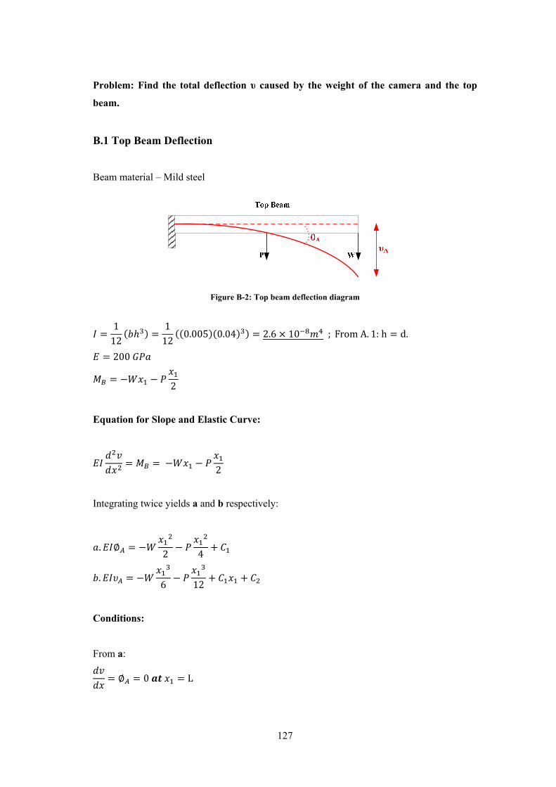
127

Problem: Find the total deflection υ caused by the weight of the camera and the top

beam.

B.1 Top Beam Deflection

Beam material – Mild steel

Figure B-2: Top beam deflection diagram

1

12

1

120.005 0.04 2.6 10   ;  From A. 1: h d.

200 

2 

Equation for Slope and Elastic Curve:

 2

Integrating twice yields a and b respectively:

. ∅2 4

.6 12

Conditions:

From a:

∅ 0    L 

128

2 4 

 

From b: 

 

0   

2  6 12

a and b becomes:

. ∅2 4 2 4

.6 12 2 4 6 12 2 4

  :      

L=400 mm

For W and P values refer to Appendix A.1.

Slope:

. ∅2 4

0.84 

∅0.84

0.00016 

Displacement:

. 0.225

0.000043  0.043  0.043 

129

B.2 Vertical Tubular Bar Deflection

Vertical bar material = Mild steel

Figure B-3: Vertical bar deflection diagram

Find dimensions in Appendix A.2.

From Appendix A.2: h=d, for the calculation to follow.

Assumptions: For worst case, only tubular bar 1 was computed. Tubular bar 2 was therefore

ignored in the calculations. Support 2 was also neglected.

1

12

1

120.032 0.032

1

120.028 0.028 3.6 10

200 

Moment about point B for x1 = L = 0.4 m:

130

24.22  .

Slope and elastic curve:

  4.22

Integrating twice yields a:

. ∅ 4.22  

Conditions:

From a:

∅ 0    H 

4.22  

a becomes:

. ∅   4.22 4.22

  :      

H=2.5 m

Slope:

. ∅ 4.22 10.55

∅10.55

0.0015 

B.3 Total Slope and deflection of the camera at point A:

From B.1 and B.2:

∅ ∅ ∅ 0.0017 

∅ . 0.000043 0.0015 0.4 0.00064  0.64   

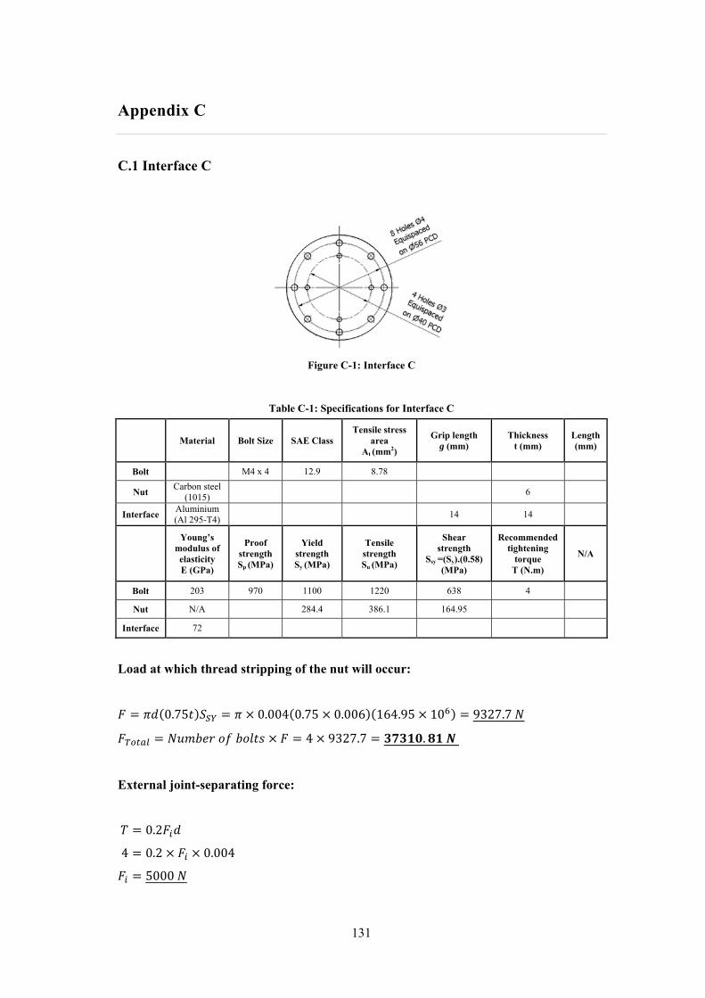
131

Appendix C

C.1 Interface C

Table C-1: Specifications for Interface C

Material Bolt Size SAE Class Tensile stress

area At (mm2)

Grip length g (mm)

Thickness t (mm)

Length (mm)

Bolt M4 x 4 12.9 8.78   

Nut Carbon steel

(1015) 6   

Interface Aluminium (Al 295-T4) 14 14   

Young’s modulus of elasticity E (GPa)

Proof strength Sp (MPa)

Yield strength Sy (MPa)

Tensile strength Su (MPa)

Shear strength

Ssy =(Sy).(0.58) (MPa)

Recommended tightening

torque T (N.m)

N/A

Bolt 203 970 1100 1220 638 4   

Nut N/A 284.4 386.1 164.95   

Interface 72   

Load at which thread stripping of the nut will occur:

0.75 0.004 0.75 0.006 164.95 10 9327.7 

    4 9327.7 .     

External joint-separating force:

0.2

4 0.2 0.004

5000 

Figure C-1: Interface C

132

0.68 0.065    0.004 0.68 0.004 0.014 0.065 0.014   

6.68 10

  8.78 10 203 10

0.01412731 10

6.68 10 72 10

0.01434354.29 10

12731 10 34354.29 10

34354.29 105000  6852.9 

    4 6852.9 .  

Maximum shear force per bolt:

0.004

4638 10 .  

C.2 Interface a for Two Finger Gripper

Only two M5 bolts where used to form the interface.

Figure C-2: Interface a for the 2-Finger parallel gripper module

133

Table C-2: Interface a specifications for the 2-Finger parallel gripper

Material Bolt Size SAE Class Tensile

stress area At (mm2)

Grip length g (mm)

Thickness t (mm)

Bolt M5 x 2 12.9 14.2

Nut Aluminium (Al 295-T4) 9

Interface Aluminium (Al 295-T4) 16 21

Length (mm)

Young’s modulus of elasticity E (GPa)

Proof strength Sp (MPa)

Yield strength Sy (MPa)

Tensile strength Su (MPa)

Shear strength

Ssy =(Sy).(0.58) (MPa)

Bolt 25 203 970 1100 1220 638

Nut 72 110 220 63.8

Interface 72

Load at which thread stripping of the nut will occur:

0.75 0.005 0.75 0.009 63.8 10 6764.63 

    2 6764.63 .     

External joint-separating force:

0.9 14.2 10 970 10 12396.6       

0.68 0.065    0.005 0.68 0.005 0.016 0.065 0.016   

9.6 10

  14.2 10 203 10

0.016180162500

9.6 10 72 10

0.016432000000

180162500 432000000

43200000012396.6 17566.5 

    2 17566.5  

Recommended bolt tightening torque:

0.2

0.2 12396.6 0.005 .   .     

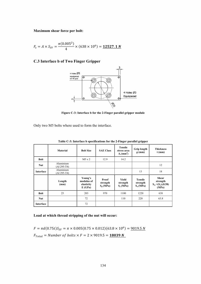
134

Maximum shear force per bolt:

0.005

4638 10 .  

C.3 Interface b of Two Finger Gripper

Only two M5 bolts where used to form the interface.

Table C-3: Interface b specifications for the 2-Finger parallel gripper

Material Bolt Size SAE Class Tensile

stress area At (mm2)

Grip length g (mm)

Thickness t (mm)

Bolt M5 x 2 12.9 14.2

Nut Aluminium (Al 295-T4) 12

Interface Aluminium (Al 295-T4) 13 18

Length (mm)

Young’s modulus of elasticity E (GPa)

Proof strength Sp (MPa)

Yield strength Sy (MPa)

Tensile strength Su (MPa)

Shear strength

Ssy =(Sy).(0.58) (MPa)

Bolt 25 203 970 1100 1220 638

Nut 72 110 220 63.8

Interface 72

Load at which thread stripping of the nut will occur:

0.75 0.005 0.75 0.012 63.8 10 9019.5 

    2 9019.5     

Figure C-3: Interface b for the 2-Finger parallel gripper module

135

External joint-separating force:

0.9 14.2 10 970 10 12396.6       

0.68 0.065    0.005 0.68 0.005 0.013 0.065 0.013   

8.02 10

  14.2 10 203 10

0.013221738461.5               

8.02 10 72 10

0.013444184615.4

221738461.5 444184615.4

444184615.412396.6 18585 

    2 18585  

Recommended bolt tightening torque:

0.2

0.2 12396.6 0.005 .   .     

Maximum shear force per bolt:

0.005

4638 10 .  

C.4 Interface a + b for Two Finger Gripper

Table C-4: Interface a + b specifications for the 2-Finger parallel gripper

Material Bolt Size SAE Class

Tensile stress area

At (mm2)

Grip length g (mm)

Thickness t (mm)

Bolt M3 x 4 12.9 5.03

Nut Same as bolt 2.3

Interface Aluminium (Al 295-T4) 36.2 39

Length (mm)

Young’s modulus of elasticity E (GPa)

Proof strength Sp (MPa)

Yield strength Sy (MPa)

Tensile strength Su (MPa)

Shear strength Ssy =(Sy).(0.58)

(MPa)

Bolt 40 203 970 1100 1220 638

Nut 203 1100 1220 638

Interface 72

136

Load at which thread stripping of the nut will occur:

0.75 0.003 0.75 0.0023 638 10 10372.44 

    4 10372.44 .     

External joint-separating force:

0.9 5.03 10 970 10 4391.2       

0.68 0.065    0.003 0.68 0.003 0.0362 0.065 0.0362   

1.68 10

  5.03 10 203 10

0.036228206906.1

1.68 10 72 10

0.0362334143646.4

28206906.1 334143646.4

334143646.44391.2 4761.9 

    4 4761.9 .  

Recommended bolt tightening torque:

0.2

0.2 4391.2 0.003 .   .     

Maximum shear stress:

0.003

4638 10 .  

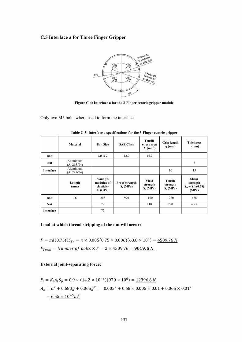
137

C.5 Interface a for Three Finger Gripper

Only two M5 bolts where used to form the interface.

Table C-5: Interface a specifications for the 3-Finger centric gripper

Material Bolt Size SAE Class Tensile

stress area At (mm2)

Grip length g (mm)

Thickness t (mm)

Bolt M5 x 2 12.9 14.2

Nut Aluminium (Al 295-T4)

6

Interface Aluminium (Al 295-T4)

10 15

Length (mm)

Young’s modulus of elasticity E (GPa)

Proof strength Sp (MPa)

Yield strength Sy (MPa)

Tensile strength Su (MPa)

Shear strength

Ssy =(Sy).(0.58) (MPa)

Bolt 16 203 970 1100 1220 638

Nut 72 110 220 63.8

Interface 72

Load at which thread stripping of the nut will occur:

0.75 0.005 0.75 0.006 63.8 10 4509.76 

    2 4509.76 .     

External joint-separating force:

0.9 14.2 10 970 10 12396.6       

0.68 0.065    0.005 0.68 0.005 0.01 0.065 0.01   

6.55 10

Figure C-4: Interface a for the 3-Finger centric gripper module

138

  14.2 10 203 10

0.01288260000

6.55 10 72 10

0.01471600000

288260000 471600000

47160000012396.6 19973.88 

    2 19973.88 .  

Recommended bolt tightening torque:

0.2

0.2 12396.6 0.005 .   .     

Maximum shear force per bolt:

0.005

4638 10 .  

C.6 Interface b of Three Finger Gripper

Table C-6: Interface b specifications for the 3-Finger centric gripper

Figure C-5: Interface b for the 3-Finger centric gripper module

139

Material Bolt Size SAE Class Tensile

stress area At (mm2)

Grip length g (mm)

Thickness t (mm)

Bolt M6 x 3 12.9 20.1

Nut Aluminium (Al 295-T4)

14

Interface Aluminium (Al 295-T4)

4 11

Length (mm)

Young’s modulus of elasticity E (GPa)

Proof strength Sp (MPa)

Yield strength Sy (MPa)

Tensile strength Su (MPa)

Shear strength

Ssy =(Sy).(0.58) (MPa)

Bolt 18 203 970 1100 1220 638

Nut 72 110 220 63.8

Interface 72

Load at which thread stripping of the nut will occur:

0.75 0.006 0.75 0.014 63.8 10 12627.32 

    3 12627.32 .     

External joint-separating force:

0.9 20.1 10 970 10 17547.3       

0.68 0.065    0.006 0.68 0.006 0.004 0.065 0.004   

5.34 10

  20.1 10 203 10

0.0041020075000

5.34 10 72 10

0.004961200000

1020075000 961200000

96120000017547.3 36169.4 

    3 36169.4 .  

Recommended bolt tightening torque:

0.2

0.2 17547.3 0.006 .   .     

Maximum shear force per bolt:

140

0.006

4638 10 .  

C.7 Interface a + b for Three Finger Gripper

Table C-7: Interface a + b specifications for the 3-Finger centric gripper

Material Bolt Size SAE Class

Tensile stress area

At (mm2)

Grip length g (mm)

Thickness t (mm)

Bolt M3 x 3 12.9 5.03

Nut Same as bolt 2.3

Interface Aluminium (Al 295-T4) 26 26

Length (mm)

Young’s modulus of elasticity E (GPa)

Proof strength Sp (MPa)

Yield strength Sy (MPa)

Tensile strength Su (MPa)

Shear strength Ssy =(Sy).(0.58)

(MPa)

Bolt 40 203 970 1100 1220 638

Nut 203 1100 1220 638

Interface 72

Load at which thread stripping of the nut will occur:

0.75 0.003 0.75 0.0023 638 10 10372.44 

    3 10372.44 .     

External joint-separating force:

0.9 5.03 10 970 10 4391.2       

0.68 0.065    0.003 0.68 0.003 0.026 0.065 0.026   

1.06 10

  5.03 10 203 10

0.02639272692.31

1.06 10 72 10

0.026293538461.5

39272692.31 293538461.5

293538461.54391.2  4978.7 

    3 4978.7  .  

141

Recommended bolt tightening torque:

0.2

0.2 4391.2  0.003 .   .     

Maximum shear force per bolt:

0.003

4638 10 .  

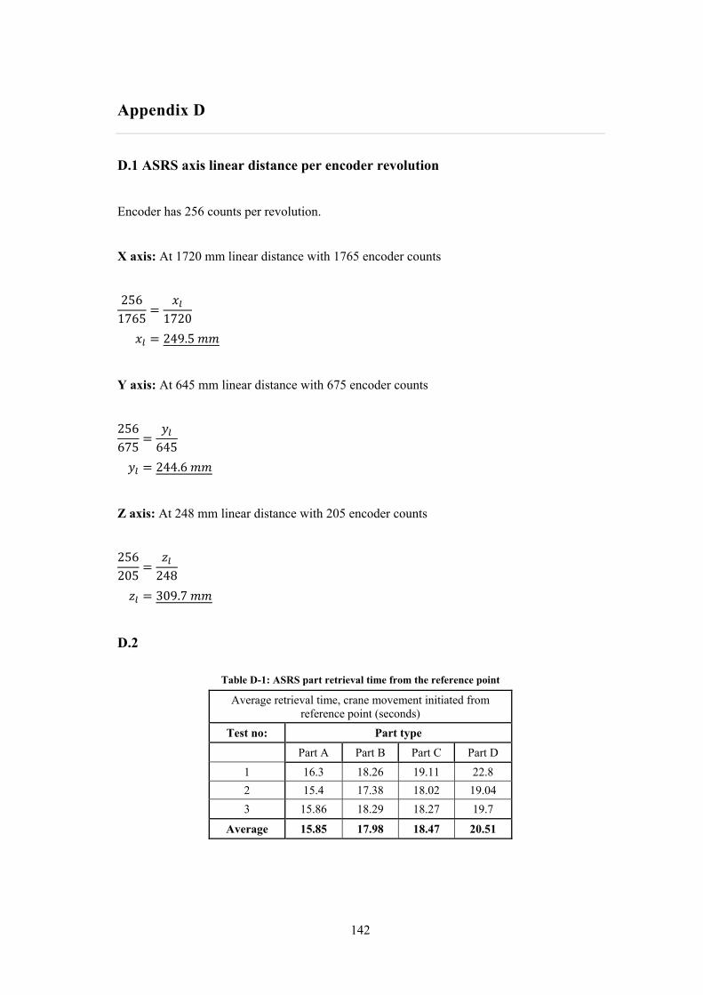
142

Appendix D

D.1 ASRS axis linear distance per encoder revolution

Encoder has 256 counts per revolution.

X axis: At 1720 mm linear distance with 1765 encoder counts

256

1765 1720

249.5 

Y axis: At 645 mm linear distance with 675 encoder counts

256

675 645

244.6 

Z axis: At 248 mm linear distance with 205 encoder counts

256

205 248

309.7 

D.2

Table D-1: ASRS part retrieval time from the reference point

Average retrieval time, crane movement initiated from reference point (seconds)

Test no: Part type

Part A Part B Part C Part D

1 16.3 18.26 19.11 22.8

2 15.4 17.38 18.02 19.04

3 15.86 18.29 18.27 19.7

Average 15.85 17.98 18.47 20.51

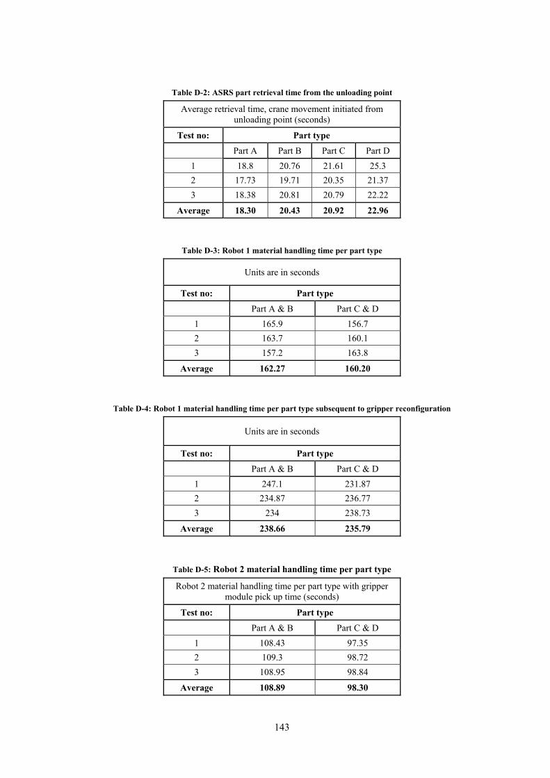
143

Table D-2: ASRS part retrieval time from the unloading point

Average retrieval time, crane movement initiated from unloading point (seconds)

Test no: Part type

Part A Part B Part C Part D

1 18.8 20.76 21.61 25.3

2 17.73 19.71 20.35 21.37

3 18.38 20.81 20.79 22.22

Average 18.30 20.43 20.92 22.96

Table D-3: Robot 1 material handling time per part type

Units are in seconds

Test no: Part type

Part A & B Part C & D

1 165.9 156.7

2 163.7 160.1

3 157.2 163.8

Average 162.27 160.20

Table D-4: Robot 1 material handling time per part type subsequent to gripper reconfiguration

Units are in seconds

Test no: Part type

Part A & B Part C & D

1 247.1 231.87

2 234.87 236.77

3 234 238.73

Average 238.66 235.79

Table D-5: Robot 2 material handling time per part type

Robot 2 material handling time per part type with gripper module pick up time (seconds)

Test no: Part type

Part A & B Part C & D

1 108.43 97.35

2 109.3 98.72

3 108.95 98.84

Average 108.89 98.30

144

Table D-6: CNC machine changeover matrix

Machine changeover time (minutes) between part types

Part Type A B C D

A 0 0 30 30

B 0 0 30 30

C 30 30 0 0

D 30 30 0 0

D.3 Conveyor speeds

Table D-7: Part travel time for conveyor 1 & 2

Units are in seconds

Test no: Conveyor 1 Conveyor 2

1 11.49 61

2 12.11 57.85

3 11.49 56.74

Average 11.70 58.53

Speed of conveyor 1:

Radius (r) = 1 m

Part travel time was taken for a quarter circle = 11.7 seconds

Circumference of the semi circular conveyor:

1 3.14 

3.14

21.57             

1.57

11.70.13  ⁄

Speed of conveyor 2:

Part travel distance = 1.05 m

Time to travel this distance = 58.53 seconds

1.05

58.530.018  ⁄

145

Appendix E

E.1 Embedded Atmega32L C code for ASRS axis position control

X axis:

#include <avr/io.h> #include <avr/interrupt.h> #include <stdio.h> #include <inttypes.h> #include "global.h" // include global settings #include "uart.h" // include uart function library #include "timer.h" #include "rprintf.h" // include printf function library #include "vt100.h" // include VT100 terminal support #include "buffer.h" #include <util/delay.h> #define horizone 0x01 // value for storage point 1 #define horiztwo 0x02 // value for storage point 2 #define horizthree 0x04 // value for storage point 3 #define horizfour 0x08 // value for storage point 4 #define horizfive 0x10 // value for storage point 5 #define reverse 0x20 // value to reverse crane #define horizdrop 0x40 // value to move crane to x-axis drop of zone #define reset 0x80 // value to reset variables to initial value uint16_t count=0; // initial value of encoder pulses short int k=0; // initial variable values short int l=0; short int m=0; short int n=0; short int p=0; short int q=0; short int r=0; short int s=0; void Init (void) { DDRB= 0xFF; // Port B set to outputs PORTB=0x00; // Port B pins all low DDRA=0x00; // Port A set to inputs DDRC=0x00; // Port C set to inputs MCUCR=0b00000010; // The falling edge of INT0 generates an interrupt request. GICR=0b01000000; // General Interrupt Control Register controls the placement of the Interrupt

//Vector sei(); // Enable interrupts } ISR(INT0_vect) // external interupt { count++;

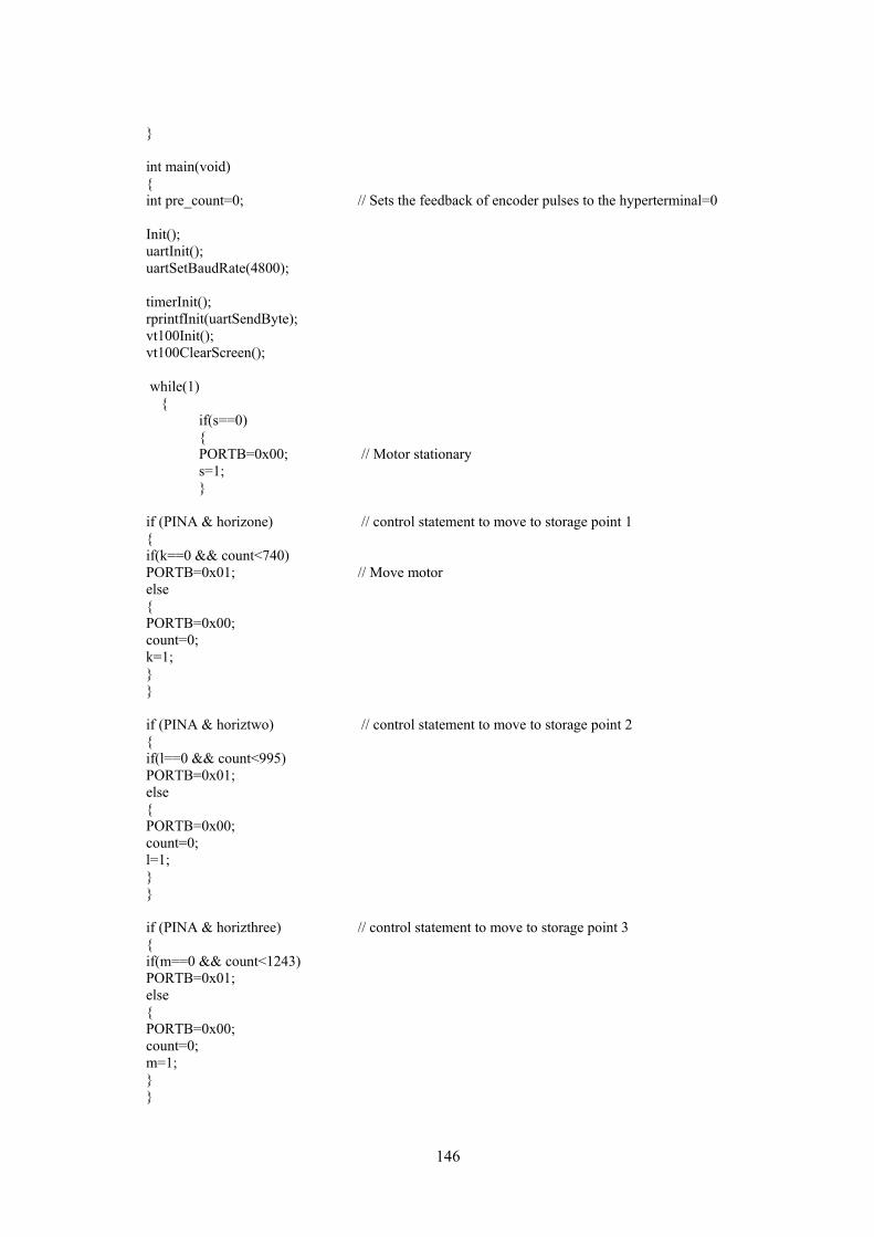
146

} int main(void) { int pre_count=0; // Sets the feedback of encoder pulses to the hyperterminal=0 Init(); uartInit(); uartSetBaudRate(4800); timerInit(); rprintfInit(uartSendByte); vt100Init(); vt100ClearScreen(); while(1) { if(s==0) { PORTB=0x00; // Motor stationary s=1; } if (PINA & horizone) // control statement to move to storage point 1 { if(k==0 && count<740) PORTB=0x01; // Move motor else { PORTB=0x00; count=0; k=1; } } if (PINA & horiztwo) // control statement to move to storage point 2 { if(l==0 && count<995) PORTB=0x01; else { PORTB=0x00; count=0; l=1; } } if (PINA & horizthree) // control statement to move to storage point 3 { if(m==0 && count<1243) PORTB=0x01; else { PORTB=0x00; count=0; m=1; } }

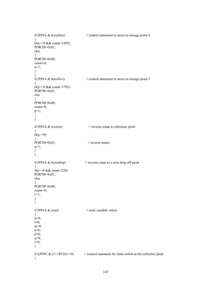
147

if (PINA & horizfour) // control statement to move to storage point 4 { if(n==0 && count<1505) PORTB=0x01; else { PORTB=0x00; count=0; n=1; } } if (PINA & horizfive) // control statement to move to storage point 5 { if(p==0 && count<1765) PORTB=0x01; else { PORTB=0x00; count=0; p=1; } } if (PINA & reverse) // reverse crane to reference point { if(q==0) { PORTB=0x03; // reverse motor q=1; } } if (PINA & horizdrop) // reverse crane to x axis drop off point { if(r==0 && count<220) PORTB=0x01; else { PORTB=0x00; count=0; r=1; } } if (PINA & reset) // reset variable values { k=0; l=0; m=0; n=0; p=0; q=0; r=0; } if ((PINC & (1<<PC0))==0) // control statement for limit switch at the reference point {

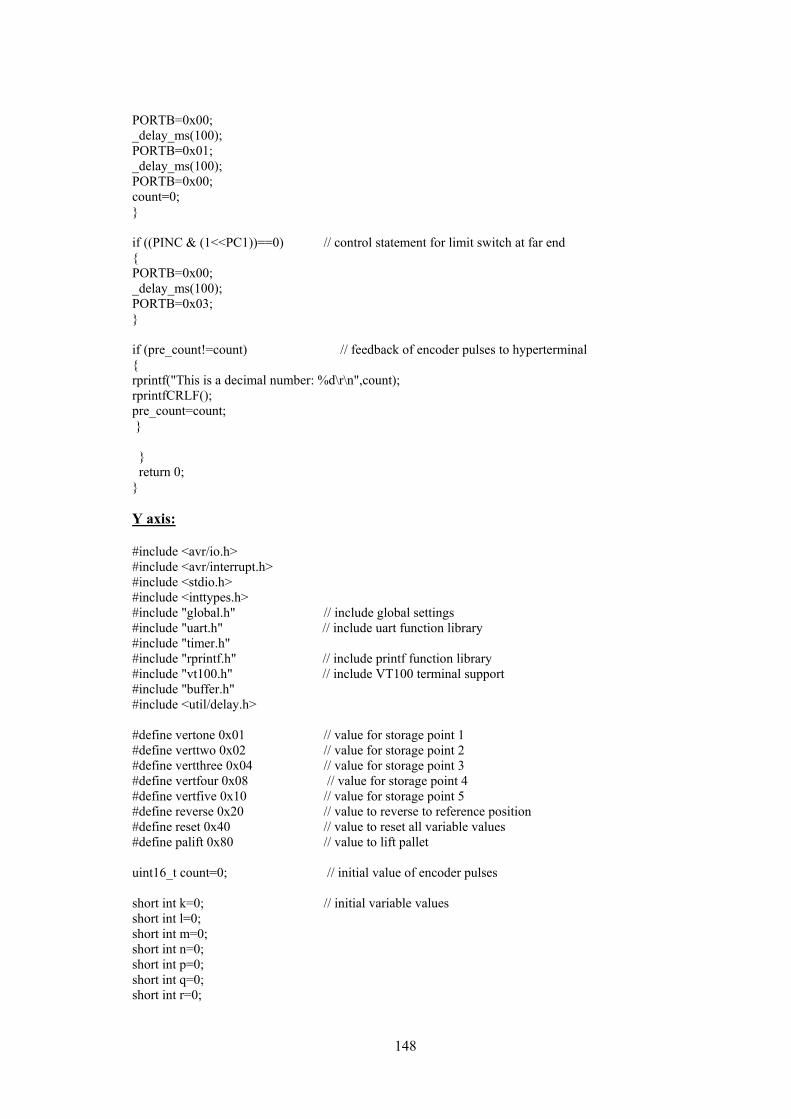
148

PORTB=0x00; _delay_ms(100); PORTB=0x01; _delay_ms(100); PORTB=0x00; count=0; } if ((PINC & (1<<PC1))==0) // control statement for limit switch at far end { PORTB=0x00; _delay_ms(100); PORTB=0x03; } if (pre_count!=count) // feedback of encoder pulses to hyperterminal { rprintf("This is a decimal number: %d\r\n",count); rprintfCRLF(); pre_count=count; } } return 0; } Y axis: #include <avr/io.h> #include <avr/interrupt.h> #include <stdio.h> #include <inttypes.h> #include "global.h" // include global settings #include "uart.h" // include uart function library #include "timer.h" #include "rprintf.h" // include printf function library #include "vt100.h" // include VT100 terminal support #include "buffer.h" #include <util/delay.h> #define vertone 0x01 // value for storage point 1 #define verttwo 0x02 // value for storage point 2 #define vertthree 0x04 // value for storage point 3 #define vertfour 0x08 // value for storage point 4 #define vertfive 0x10 // value for storage point 5 #define reverse 0x20 // value to reverse to reference position #define reset 0x40 // value to reset all variable values #define palift 0x80 // value to lift pallet uint16_t count=0; // initial value of encoder pulses short int k=0; // initial variable values short int l=0; short int m=0; short int n=0; short int p=0; short int q=0; short int r=0;

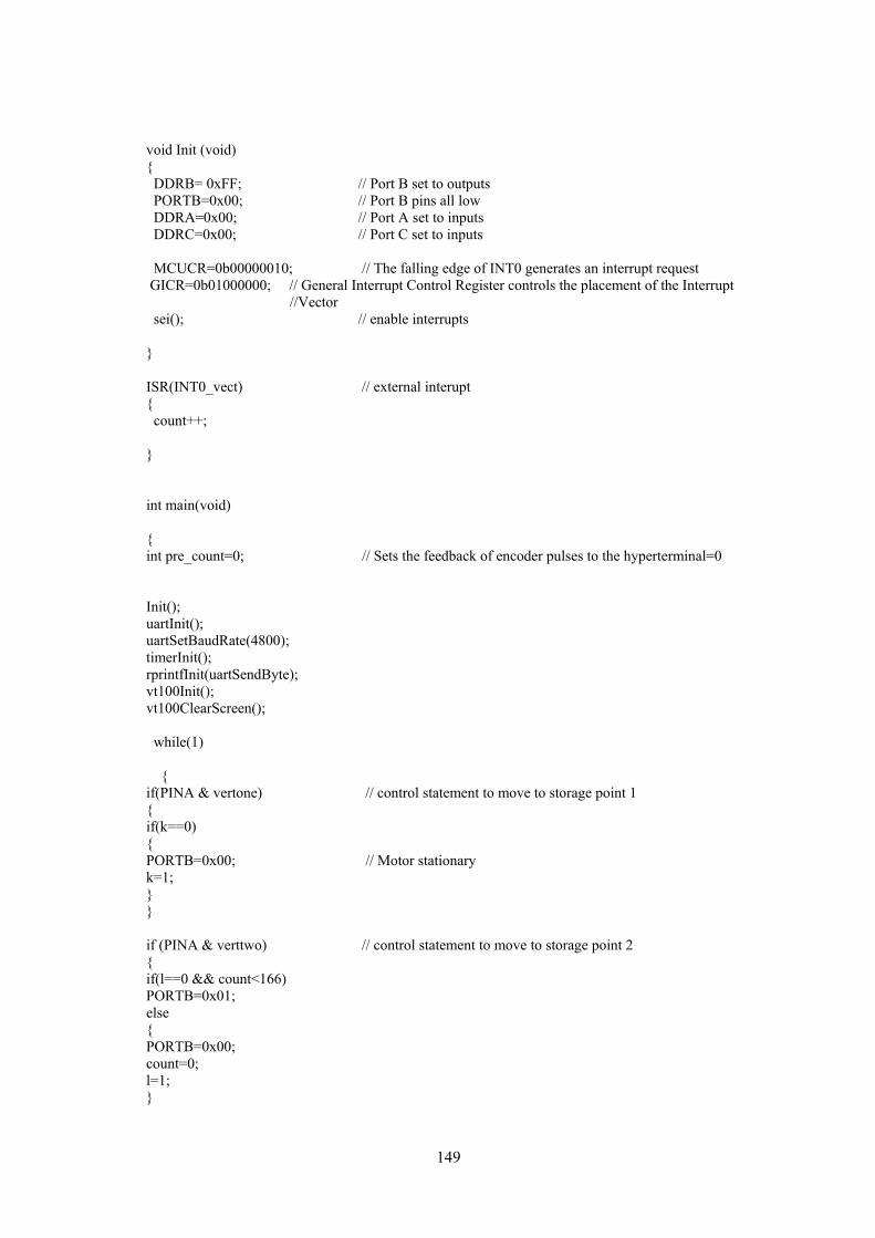
149

void Init (void) { DDRB= 0xFF; // Port B set to outputs PORTB=0x00; // Port B pins all low DDRA=0x00; // Port A set to inputs DDRC=0x00; // Port C set to inputs MCUCR=0b00000010; // The falling edge of INT0 generates an interrupt request GICR=0b01000000; // General Interrupt Control Register controls the placement of the Interrupt //Vector sei(); // enable interrupts } ISR(INT0_vect) // external interupt { count++; } int main(void) { int pre_count=0; // Sets the feedback of encoder pulses to the hyperterminal=0 Init(); uartInit(); uartSetBaudRate(4800); timerInit(); rprintfInit(uartSendByte); vt100Init(); vt100ClearScreen(); while(1) { if(PINA & vertone) // control statement to move to storage point 1 { if(k==0) { PORTB=0x00; // Motor stationary k=1; } } if (PINA & verttwo) // control statement to move to storage point 2 { if(l==0 && count<166) PORTB=0x01; else { PORTB=0x00; count=0; l=1; }

150

} if (PINA & vertthree) // control statement to move to storage point 3 { if(m==0 && count<330) PORTB=0x01; else { PORTB=0x00; count=0; m=1; } } if (PINA & vertfour) // control statement to move to storage point 4 { if(n==0 && count<500) PORTB=0x01; else { PORTB=0x00; count=0; n=1; } } if (PINA & vertfive) // control statement to move to storage point 5 { if(p==0 && count<675) PORTB=0x01; else {PORTB=0x00; count=0; p=1; } } if (PINA & palift) // control statement to lift pallet in Y direction { if (r==0 && count<30) PORTB=0x01; else { PORTB=0x00; count=0; r=1; } } if (PINA & reset) // reset variable values { k=0; l=0; m=0; n=0; p=0; q=0; r=0;

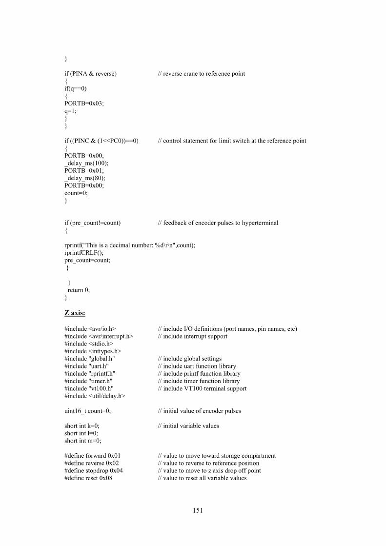
151

} if (PINA & reverse) // reverse crane to reference point { if(q==0) { PORTB=0x03; q=1; } } if ((PINC & (1<<PC0))==0) // control statement for limit switch at the reference point { PORTB=0x00; _delay_ms(100); PORTB=0x01; _delay_ms(80); PORTB=0x00; count=0; } if (pre_count!=count) // feedback of encoder pulses to hyperterminal { rprintf("This is a decimal number: %d\r\n",count); rprintfCRLF(); pre_count=count; } } return 0; } Z axis: #include <avr/io.h> // include I/O definitions (port names, pin names, etc) #include <avr/interrupt.h> // include interrupt support #include <stdio.h> #include <inttypes.h> #include "global.h" // include global settings #include "uart.h" // include uart function library #include "rprintf.h" // include printf function library #include "timer.h" // include timer function library #include "vt100.h" // include VT100 terminal support #include <util/delay.h> uint16_t count=0; // initial value of encoder pulses short int k=0; // initial variable values short int l=0; short int m=0; #define forward 0x01 // value to move toward storage compartment #define reverse 0x02 // value to reverse to reference position #define stopdrop 0x04 // value to move to z axis drop off point #define reset 0x08 // value to reset all variable values

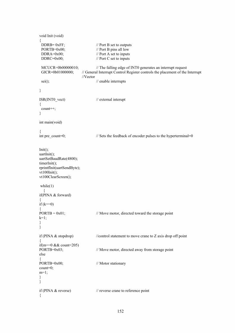
152

void Init (void) { DDRB= 0xFF; // Port B set to outputs PORTB=0x00; // Port B pins all low DDRA=0x00; // Port A set to inputs DDRC=0x00; // Port C set to inputs MCUCR=0b00000010; // The falling edge of INT0 generates an interrupt request GICR=0b01000000; // General Interrupt Control Register controls the placement of the Interrupt //Vector sei(); // enable interrupts } ISR(INT0_vect) // external interupt { count++; } int main(void) { int pre_count=0; // Sets the feedback of encoder pulses to the hyperterminal=0 Init(); uartInit(); uartSetBaudRate(4800); timerInit(); rprintfInit(uartSendByte); vt100Init(); vt100ClearScreen(); while(1) { if(PINA & forward) { if (k==0) { PORTB = 0x01; // Move motor, directed toward the storage point k=1; } } if (PINA & stopdrop) //control statement to move crane to Z axis drop off point { if(m==0 && count<205) PORTB=0x03; // Move motor, directed away from storage point else { PORTB=0x00; // Motor stationary count=0; m=1; } } if (PINA & reverse) // reverse crane to reference point {

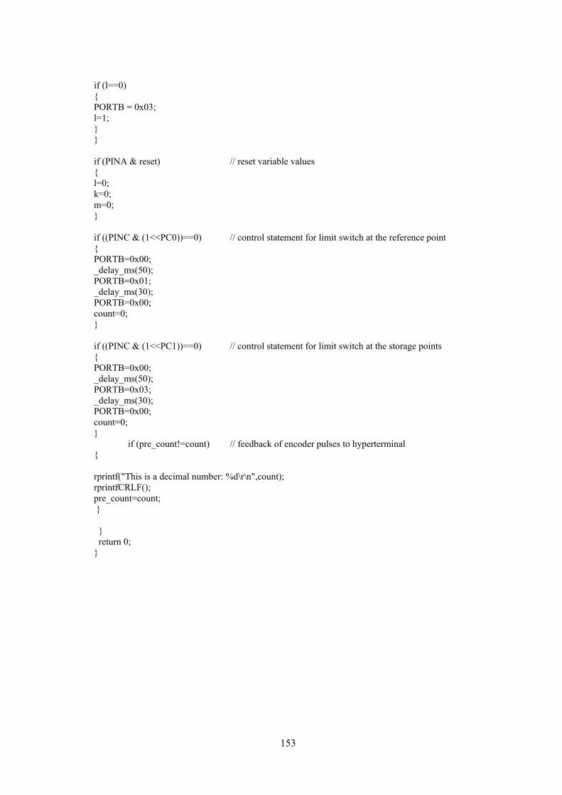
153

if (l==0) { PORTB = 0x03; l=1; } } if (PINA & reset) // reset variable values { l=0; k=0; m=0; } if ((PINC & (1<<PC0))==0) // control statement for limit switch at the reference point { PORTB=0x00; _delay_ms(50); PORTB=0x01; _delay_ms(30); PORTB=0x00; count=0; } if ((PINC & (1<<PC1))==0) // control statement for limit switch at the storage points { PORTB=0x00; _delay_ms(50); PORTB=0x03; _delay_ms(30); PORTB=0x00; count=0; } if (pre_count!=count) // feedback of encoder pulses to hyperterminal { rprintf("This is a decimal number: %d\r\n",count); rprintfCRLF(); pre_count=count; } } return 0; }

154

E.2 Visual Basic code

Master Control Program (MCP):

Option Explicit Dim Err As Long ' write function variable for uDAQ Dim Err2 As Long ' write function variable for uDAQLite Dim Err3 As Long ' read function variable for uDAQLite Dim serialnum As Long 'uDAQ serial number Dim serialnum2 As Long ' uDAQLite serial number Dim r As Long Dim s As Boolean Private Declare Sub Sleep Lib "kernel32" (ByVal dwMilliseconds As Long) Private Sub execprod_Click() Dim PTA As Double ' total CNC processing time for customer order A Dim A As Double Dim timeA As Long 'time to process customer order A Dim PTB As Double ' total CNC processing time for customer order B Dim B As Double Dim timeB As Long 'time to process customer order B Dim PTC As Double ' total CNC processing time for customer order C Dim C As Double Dim timeC As Long 'time to process customer order C Dim PTD As Double ' total CNC processing time for customer order D Dim D As Double Dim timeD As Long 'time to process customer order D Dim numA As Integer Dim numB As Integer Dim numC As Integer Dim numD As Integer serialnum = 1000010732 numA = Text5.Text numB = Text6.Text numC = Text7.Text numD = Text8.Text PTA = 16.09 * numA PTB = 8.513 * numB PTC = 13.807 * numC PTD = 8.79 * numD DoEvents Sleep (100) timeA = Text1.Text A = Divide(timeA, PTA) Label1.Caption = A timeB = Text2.Text B = Divide(timeB, PTB) Label2.Caption = B

155

timeC = Text3.Text C = Divide(timeC, PTC) Label3.Caption = C timeD = Text4.Text D = Divide(timeD, PTD) Label4.Caption = D Sleep (2000) DoEvents Call reset '''''''''''''''''''''''''''''''''''''''''''''''''''''''''''''''''''''''''''''''''''''' If A < B And B < C And C < D Then Call linespace Print "Execute order A" Print "Execute order B" Print "Execute order C" Print "Execute order D" DoEvents 'A Call productA 'B Call productB 'C Call productC 'D Call productD DoEvents End If ''''''''''''''''''''''''''''''''''''''''''''''''''''''''''''''''''''''''''''''''''''' If A < B And B < D And D < C Then Call linespace Print "Execute order A" Print "Execute order B" Print "Execute order D" Print "Execute order C" DoEvents 'A Call productA 'B Call productB 'D Call productD 'C Call productC DoEvents End If ''''''''''''''''''''''''''''''''''''''''''''''''''''''''''''''''''''''''''''''''''''' If A < C And C < B And B < D Then Call linespace Print "Execute order A" Print "Execute order C" Print "Execute order B" Print "Execute order D" DoEvents 'A Call productA 'C Call productC

156

'B Call productB 'D Call productD DoEvents End If ''''''''''''''''''''''''''''''''''''''''''''''''''''''''''''''''''''''''''''''''''' If A < C And C < D And D < B Then Call linespace Print "Execute order A" Print "Execute order C" Print "Execute order D" Print "Execute order B" DoEvents 'A Call productA 'C Call productC 'D Call productD 'B Call productB DoEvents End If '''''''''''''''''''''''''''''''''''''''''''''''''''''''''''''''''''''''''''''''''''' If A < D And D < B And B < C Then Call linespace Print "Execute order A" Print "Execute order D" Print "Execute order B" Print "Execute order C" DoEvents 'A Call productA 'D Call productD 'B Call productB 'C Call productC DoEvents End If '''''''''''''''''''''''''''''''''''''''''''''''''''''''''''''''''''''''''''''''''''' If A < D And D < C And C < B Then Call linespace Print "Execute order A" Print "Execute order D" Print "Execute order C" Print "Execute order B" DoEvents 'A Call productA 'D Call productD 'C Call productC 'B Call productB

157

DoEvents End If ''''''''''''''''''''''''''''''''''''''''''''''''''''''''''''''''''''''''''''''''''' If B < A And A < C And C < D Then Call linespace Print "Execute order B" Print "Execute order A" Print "Execute order C" Print "Execute order D" DoEvents 'B Call productB 'A Call productA 'C Call productC 'D Call productD DoEvents End If ''''''''''''''''''''''''''''''''''''''''''''''''''''''''''''''''''''''''''''''''''' If B < A And A < D And D < C Then Call linespace Print "Execute order B" Print "Execute order A" Print "Execute order D" Print "Execute order C" DoEvents 'B Call productB 'A Call productA 'D Call productD 'C Call productC DoEvents End If '''''''''''''''''''''''''''''''''''''''''''''''''''''''''''''''''''''''''''''''''' If B < C And C < A And A < D Then Call linespace Print "Execute order B" Print "Execute order C" Print "Execute order A" Print "Execute order D" DoEvents 'B Call productA 'C Call productA 'A Call productA 'D Call productA DoEvents End If '''''''''''''''''''''''''''''''''''''''''''''''''''''''''''''''''''''''''''''''''

158

If B < C And C < D And D < A Then Call linespace Print "Execute order B" Print "Execute order C" Print "Execute order D" Print "Execute order A" DoEvents 'B Call productB 'C Call productC 'D Call productD 'A Call productA DoEvents End If ''''''''''''''''''''''''''''''''''''''''''''''''''''''''''''''''''''''''''''''''' If B < D And D < A And A < C Then Call linespace Print "Execute order B" Print "Execute order D" Print "Execute order A" Print "Execute order C" DoEvents 'B Call productB 'D Call productD 'A Call productA 'C Call productC DoEvents End If ''''''''''''''''''''''''''''''''''''''''''''''''''''''''''''''''''''''''''''''''' If B < D And D < C And C < A Then Call linespace Print "Execute order B" Print "Execute order D" Print "Execute order C" Print "Execute order A" DoEvents 'B Call productB 'D Call productD 'C Call productC 'A Call productA DoEvents End If '''''''''''''''''''''''''''''''''''''''''''''''''''''''''''''''''''''''''''''''' If C < A And A < B And B < D Then Call linespace Print "Execute order C"

159

Print "Execute order A" Print "Execute order B" Print "Execute order D" DoEvents 'C Call productC 'A Call productA 'B Call productB 'D Call productD DoEvents End If '''''''''''''''''''''''''''''''''''''''''''''''''''''''''''''''''''''''''''''''' If C < A And A < D And D < B Then Call linespace Print "Execute order C" Print "Execute order A" Print "Execute order D" Print "Execute order B" DoEvents 'C Call productC 'A Call productA 'D Call productD 'B Call productB DoEvents End If '''''''''''''''''''''''''''''''''''''''''''''''''''''''''''''''''''''''''''''''' If C < B And B < A And A < D Then Call linespace Print "Execute order C" Print "Execute order B" Print "Execute order A" Print "Execute order D" DoEvents 'C Call productC 'B Call productB 'A Call productA 'D Call productD DoEvents End If ''''''''''''''''''''''''''''''''''''''''''''''''''''''''''''''''''''''''''''' If C < B And B < D And D < A Then Call linespace Print "Execute order C" Print "Execute order B" Print "Execute order D" Print "Execute order A" DoEvents

160

'C Call productC 'B Call productB 'D Call productD 'A Call productA DoEvents End If ''''''''''''''''''''''''''''''''''''''''''''''''''''''''''''''''''''''''''''' If C < D And D < A And A < B Then Call linespace Print "Execute order C" Print "Execute order D" Print "Execute order A" Print "Execute order B" DoEvents 'C Call productC 'D Call productD 'A Call productA 'B Call productB DoEvents End If '''''''''''''''''''''''''''''''''''''''''''''''''''''''''''''''''''''''''''' If C < D And D < B And B < A Then Call linespace Print "Execute order C" Print "Execute order D" Print "Execute order B" Print "Execute order A" DoEvents 'C Call productC 'D Call productD 'B Call productB 'A Call productA DoEvents End If '''''''''''''''''''''''''''''''''''''''''''''''''''''''''''''''''''''''''''' If D < A And A < B And B < C Then Call linespace Print "Execute order D" Print "Execute order A" Print "Execute order B" Print "Execute order C" DoEvents 'D Call productD 'A Call productA

161

'B Call productB 'C Call productC DoEvents End If ''''''''''''''''''''''''''''''''''''''''''''''''''''''''''''''''''''''''''' If D < A And A < C And C < B Then Call linespace Print "Execute order D" Print "Execute order A" Print "Execute order C" Print "Execute order B" DoEvents 'D Call productD 'A Call productA 'C Call productC 'B Call productB DoEvents End If ''''''''''''''''''''''''''''''''''''''''''''''''''''''''''''''''''''''''''' If D < B And B < A And A < C Then Call linespace Print "Execute order D" Print "Execute order B" Print "Execute order A" Print "Execute order C" DoEvents 'D Call productD 'B Call productB 'A Call productA 'C Call productC DoEvents End If ''''''''''''''''''''''''''''''''''''''''''''''''''''''''''''''''''''''''''' If D < B And B < C And C < A Then Call linespace Print "Execute order D" Print "Execute order B" Print "Execute order C" Print "Execute order A" DoEvents 'D Call productD 'B Call productB 'C Call productC 'A Call productA

162

DoEvents End If '''''''''''''''''''''''''''''''''''''''''''''''''''''''''''''''''''''''''''' If D < C And C < A And A < B Then Call linespace Print "Execute order D" Print "Execute order C" Print "Execute order A" Print "Execute order B" DoEvents 'D Call productD 'C Call productC 'A Call productA 'B Call productB DoEvents End If '''''''''''''''''''''''''''''''''''''''''''''''''''''''''''''''''''''''''''' If D < C And C < B And B < A Then Call linespace Print "Execute order D" Print "Execute order C" Print "Execute order B" Print "Execute order A" DoEvents 'D Call productD 'C Call productC 'B Call productB 'A Call productA DoEvents End If End Sub Private Sub reset() Err = EDRE_DioWrite(serialnum, 0, 128) 'X_Axis_ResetAllPinsOnPort0 Sleep (100) DoEvents Err = EDRE_DioWrite(serialnum, 0, 0) 'X_Axis_ResetPort0ToZero Sleep (100) DoEvents Err = EDRE_DioWrite(serialnum, 3, 64) 'Y_Axis_ResetAllPinsOnPort3 Sleep (100) DoEvents Err = EDRE_DioWrite(serialnum, 3, 0) 'Y_Axis_ResetPort3ToZero Sleep (100) DoEvents Err = EDRE_DioWrite(serialnum, 6, 8) 'Z_Axis_ResetAllPinsOnPort6 Sleep (100) DoEvents

163

Err = EDRE_DioWrite(serialnum, 6, 0) 'Z_Axis_ResetPort6ToZero Sleep (1000) DoEvents End Sub Private Sub similarmoves() Err = EDRE_DioWrite(serialnum, 6, 1) 'Z_Axis_MoveForwardToStoragePoint Sleep (3000) DoEvents Err = EDRE_DioWrite(serialnum, 6, 8) 'Z_Axis_ResetAllPinsOnPort6 Sleep (500) DoEvents Err = EDRE_DioWrite(serialnum, 6, 0) 'Z_Axis_ResetPort6ToZero Sleep (500) DoEvents Err = EDRE_DioWrite(serialnum, 3, 128) 'Y_Axis_PalletLift Sleep (3000) DoEvents Err = EDRE_DioWrite(serialnum, 3, 64) 'Y_Axis_ResetPort3Pins Sleep (500) DoEvents Err = EDRE_DioWrite(serialnum, 3, 0) 'Y_Axis_ResetPort3ToZero Sleep (500) DoEvents Err = EDRE_DioWrite(serialnum, 6, 4) 'Z_Axis_MoveBackwardsToDropOfPosition Sleep (2000) DoEvents Err = EDRE_DioWrite(serialnum, 6, 8) 'Z_Axis_ResetAllPinsOnPort6 Sleep (500) DoEvents Err = EDRE_DioWrite(serialnum, 6, 0) 'Z_Axis_ResetPort6ToZero Sleep (500) DoEvents Err = EDRE_DioWrite(serialnum, 0, 32) 'X_Axis_ReverseToInitialPosition Sleep (5000) DoEvents Err = EDRE_DioWrite(serialnum, 0, 128) 'X_Axis_ResetAllPinsOnPort0 Sleep (500) DoEvents Err = EDRE_DioWrite(serialnum, 0, 0) 'X_Axis_ResetPort0ToZero Sleep (500) DoEvents Err = EDRE_DioWrite(serialnum, 0, 64) 'X_Axis_GoToDropOfPosition Sleep (2000) DoEvents Err = EDRE_DioWrite(serialnum, 0, 128) 'X_Axis_ResetAllPinsOnPort0 Sleep (500) DoEvents Err = EDRE_DioWrite(serialnum, 0, 0) 'X_Axis_ResetPort0ToZero Sleep (500) DoEvents Err = EDRE_DioWrite(serialnum, 3, 32) 'Y_Axis_GoToInitialPosition Sleep (9000) DoEvents Err = EDRE_DioWrite(serialnum, 3, 64) 'Y_Axis_ResetAllPinsOnPort3 Sleep (500) DoEvents

164

Err = EDRE_DioWrite(serialnum, 3, 0) 'Y_Axis_ResetPort3ToZero Sleep (500) DoEvents End Sub Private Sub productA() Err = EDRE_DioWrite(serialnum, 0, 1) 'X_Axis_GoToColumn1 Sleep (4000) DoEvents Call reset Err = EDRE_DioWrite(serialnum, 3, 1) 'Y_Axis_GoToRow1 Sleep (1000) DoEvents Call reset Call similarmoves 'End of Retrieval Call reset End Sub Private Sub productB() Err = EDRE_DioWrite(serialnum, 0, 1) 'X_Axis_GoToColumn1 Sleep (4000) DoEvents Call reset Err = EDRE_DioWrite(serialnum, 3, 2) 'Y_Axis_GoToRow2 Sleep (1000) DoEvents Call reset Call similarmoves 'End of Retrieval Call reset End Sub Private Sub productC() Err = EDRE_DioWrite(serialnum, 0, 2) 'X_Axis_GoToColumn2 Sleep (4000) DoEvents Call reset Err = EDRE_DioWrite(serialnum, 3, 1) 'Y_Axis_GoToRow1 Sleep (1000) DoEvents Call reset Call similarmoves 'End of Retrieval Call reset End Sub Private Sub productD() Err = EDRE_DioWrite(serialnum, 0, 2) 'X_Axis_GoToColumn2 Sleep (4000) DoEvents Call reset Err = EDRE_DioWrite(serialnum, 3, 2) 'Y_Axis_GoToRow2 Sleep (1000)

165

DoEvents Call reset Call similarmoves 'End of Retrieval Call reset End Sub Private Sub startconveyor_Click() Dim v As Long serialnum2 = 1000010155 Do Until s = True DoEvents Do While v = 1 Err2 = EDRE_DioWrite(serialnum2, 0, 3) ' Conveyor motor run Err3 = EDRE_DioRead(serialnum2, 0, v) DoEvents If s = True Then Exit Do End If Loop Do While v = 0 Err2 = EDRE_DioWrite(serialnum2, 0, 4) ' Conveyor motor stop, send signal to 5/24 V step up circuit Err3 = EDRE_DioRead(serialnum2, 0, v) DoEvents If s = True Then Exit Do End If Loop If s = True Then Exit Do End If Loop s = False End Sub Public Sub stopconveyor_Click() serialnum2 = 1000010155 s = Err2 = EDRE_DioWrite(serialnum2, 0, 0) = True End Sub Private Function Divide(n As Long, D As Double) As String ' function for prioritising scheduling If n = 0 Then Exit Function Else Divide = n / D End If End Function

166

Private Sub end_Click() Call reset DoEvents Unload Me End End Sub Private Sub leaveline() Print Print Print Print Print Print Print End Sub Private Sub linespace() Print Print Print Print Print Print Print End Sub

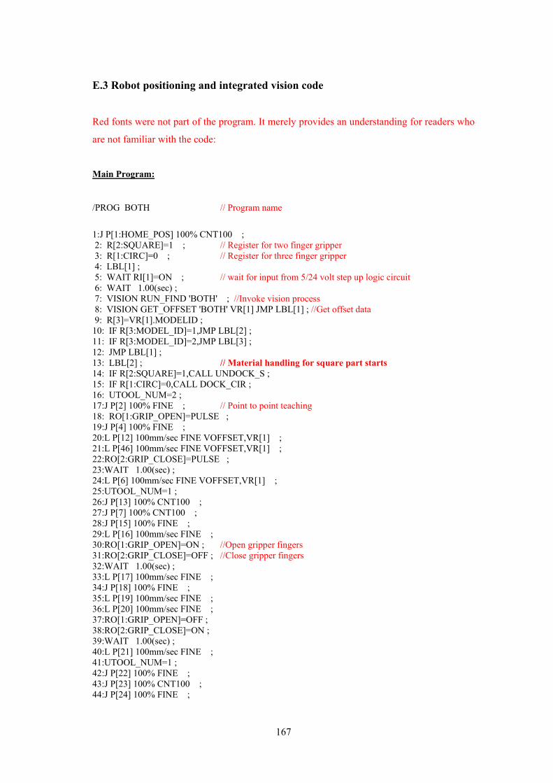
167

E.3 Robot positioning and integrated vision code

Red fonts were not part of the program. It merely provides an understanding for readers who

are not familiar with the code:

Main Program:

/PROG BOTH // Program name

1:J P[1:HOME_POS] 100% CNT100 ; 2: R[2:SQUARE]=1 ; // Register for two finger gripper 3: R[1:CIRC]=0 ; // Register for three finger gripper 4: LBL[1] ; 5: WAIT RI[1]=ON ; // wait for input from 5/24 volt step up logic circuit 6: WAIT 1.00(sec) ; 7: VISION RUN_FIND 'BOTH' ; //Invoke vision process 8: VISION GET_OFFSET 'BOTH' VR[1] JMP LBL[1] ; //Get offset data 9: R[3]=VR[1].MODELID ; 10: IF R[3:MODEL_ID]=1,JMP LBL[2] ; 11: IF R[3:MODEL_ID]=2,JMP LBL[3] ; 12: JMP LBL[1] ; 13: LBL[2] ; // Material handling for square part starts 14: IF R[2:SQUARE]=1,CALL UNDOCK_S ; 15: IF R[1:CIRC]=0,CALL DOCK_CIR ; 16: UTOOL_NUM=2 ; 17:J P[2] 100% FINE ; // Point to point teaching 18: RO[1:GRIP_OPEN]=PULSE ; 19:J P[4] 100% FINE ; 20:L P[12] 100mm/sec FINE VOFFSET,VR[1] ; 21:L P[46] 100mm/sec FINE VOFFSET,VR[1] ; 22:RO[2:GRIP_CLOSE]=PULSE ; 23:WAIT 1.00(sec) ; 24:L P[6] 100mm/sec FINE VOFFSET,VR[1] ; 25:UTOOL_NUM=1 ; 26:J P[13] 100% CNT100 ; 27:J P[7] 100% CNT100 ; 28:J P[15] 100% FINE ; 29:L P[16] 100mm/sec FINE ; 30:RO[1:GRIP_OPEN]=ON ; //Open gripper fingers 31:RO[2:GRIP_CLOSE]=OFF ; //Close gripper fingers 32:WAIT 1.00(sec) ; 33:L P[17] 100mm/sec FINE ; 34:J P[18] 100% FINE ; 35:L P[19] 100mm/sec FINE ; 36:L P[20] 100mm/sec FINE ; 37:RO[1:GRIP_OPEN]=OFF ; 38:RO[2:GRIP_CLOSE]=ON ; 39:WAIT 1.00(sec) ; 40:L P[21] 100mm/sec FINE ; 41:UTOOL_NUM=1 ; 42:J P[22] 100% FINE ; 43:J P[23] 100% CNT100 ; 44:J P[24] 100% FINE ;

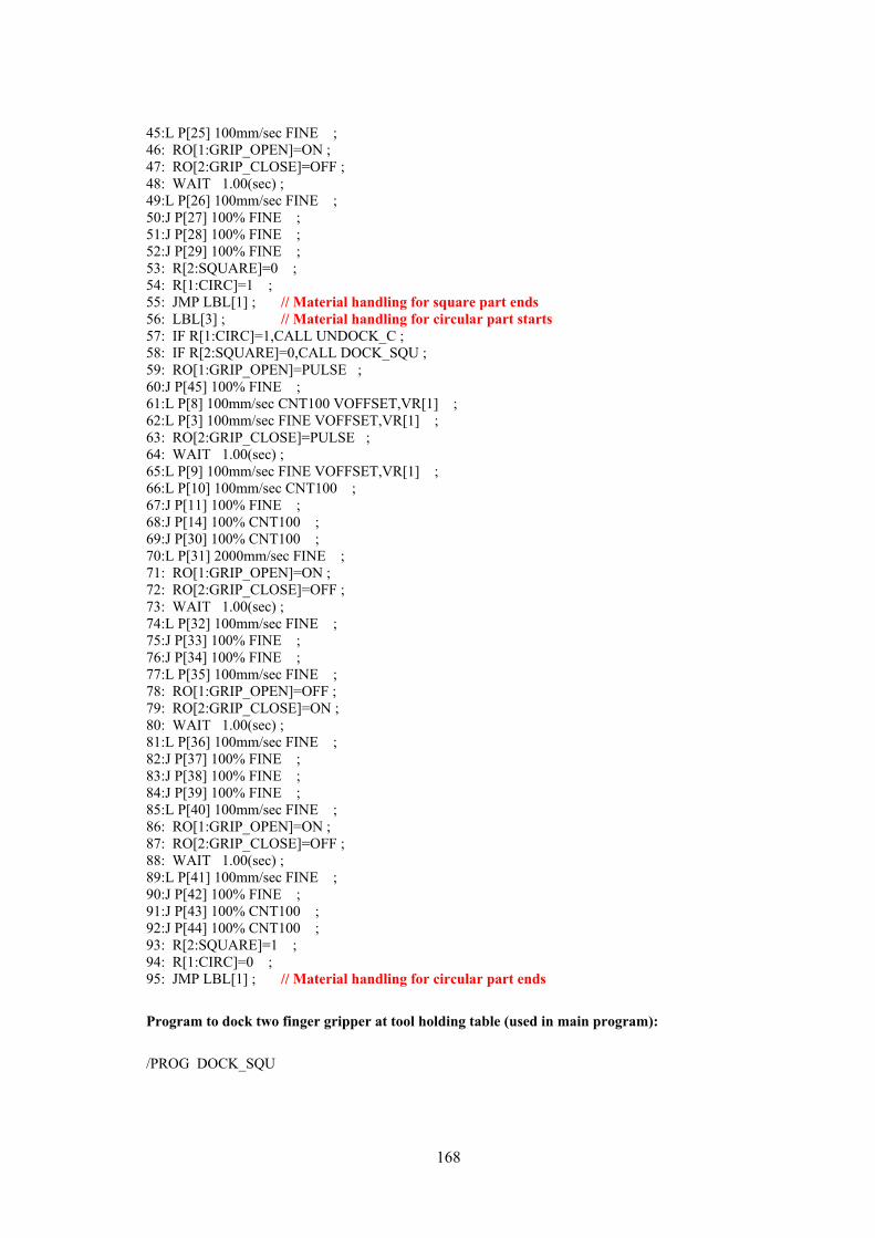
168

45:L P[25] 100mm/sec FINE ; 46: RO[1:GRIP_OPEN]=ON ; 47: RO[2:GRIP_CLOSE]=OFF ; 48: WAIT 1.00(sec) ; 49:L P[26] 100mm/sec FINE ; 50:J P[27] 100% FINE ; 51:J P[28] 100% FINE ; 52:J P[29] 100% FINE ; 53: R[2:SQUARE]=0 ; 54: R[1:CIRC]=1 ; 55: JMP LBL[1] ; // Material handling for square part ends 56: LBL[3] ; // Material handling for circular part starts 57: IF R[1:CIRC]=1,CALL UNDOCK_C ; 58: IF R[2:SQUARE]=0,CALL DOCK_SQU ; 59: RO[1:GRIP_OPEN]=PULSE ; 60:J P[45] 100% FINE ; 61:L P[8] 100mm/sec CNT100 VOFFSET,VR[1] ; 62:L P[3] 100mm/sec FINE VOFFSET,VR[1] ; 63: RO[2:GRIP_CLOSE]=PULSE ; 64: WAIT 1.00(sec) ; 65:L P[9] 100mm/sec FINE VOFFSET,VR[1] ; 66:L P[10] 100mm/sec CNT100 ; 67:J P[11] 100% FINE ; 68:J P[14] 100% CNT100 ; 69:J P[30] 100% CNT100 ; 70:L P[31] 2000mm/sec FINE ; 71: RO[1:GRIP_OPEN]=ON ; 72: RO[2:GRIP_CLOSE]=OFF ; 73: WAIT 1.00(sec) ; 74:L P[32] 100mm/sec FINE ; 75:J P[33] 100% FINE ; 76:J P[34] 100% FINE ; 77:L P[35] 100mm/sec FINE ; 78: RO[1:GRIP_OPEN]=OFF ; 79: RO[2:GRIP_CLOSE]=ON ; 80: WAIT 1.00(sec) ; 81:L P[36] 100mm/sec FINE ; 82:J P[37] 100% FINE ; 83:J P[38] 100% FINE ; 84:J P[39] 100% FINE ; 85:L P[40] 100mm/sec FINE ; 86: RO[1:GRIP_OPEN]=ON ; 87: RO[2:GRIP_CLOSE]=OFF ; 88: WAIT 1.00(sec) ; 89:L P[41] 100mm/sec FINE ; 90:J P[42] 100% FINE ; 91:J P[43] 100% CNT100 ; 92:J P[44] 100% CNT100 ; 93: R[2:SQUARE]=1 ; 94: R[1:CIRC]=0 ; 95: JMP LBL[1] ; // Material handling for circular part ends

Program to dock two finger gripper at tool holding table (used in main program):

/PROG DOCK_SQU

169

1:L P[3] 2000mm/sec FINE ; 2:L P[4] 100mm/sec FINE ; 3: RO[4:DOCK_GRIP]=OFF ; // Lock 2 finger gripper at tool holding table 4: WAIT 1.00(sec) ; 5: R[2:SQUARE]=1 ; 6:L P[5] 100mm/sec FINE ; 7:J P[6] 100% CNT100 ;

Program to dock three finger gripper at tool holding table (used in main program):

/PROG DOCK_CIR

1:J P[5] 100% FINE ; 2:L P[1] 2000mm/sec FINE ; 3:L P[2] 100mm/sec FINE ; 4: RO[4:DOCK_GRIP]=OFF ; // Lock 3 finger gripper at tool holding table 5: WAIT 1.00(sec) ; 6: R[1:CIRC]=1 ; 7:L P[3] 100mm/sec FINE ; 8:J P[4] 100% CNT100 ;

Program to undock two finger gripper at tool holding table (used in main program):

/PROG UNDOCK_S

1:J P[4] 100% FINE ; 2:L P[1] 2000mm/sec FINE ; 3: RO[1:GRIP_OPEN]=OFF ; 4: RO[2:GRIP_CLOSE]=OFF ; 5:L P[2] 100mm/sec FINE ; 6: RO[4:DOCK_GRIP]=ON ; // Unlock 2 finger gripper at tool holding table 7: WAIT 1.00(sec) ; 8: R[2:SQUARE]=0 ; 9:L P[3] 100mm/sec FINE ; 10:J P[5] 100% FINE ;

Program to undock three finger gripper at tool holding table (used in main program):

/PROG UNDOCK_C

1:J P[4] 100% FINE ; 2:L P[1] 1000mm/sec FINE ; 3: RO[1:GRIP_OPEN]=OFF ; 4: RO[2:GRIP_CLOSE]=OFF ; 5:L P[2] 100mm/sec FINE ; 6: RO[4:DOCK_GRIP]=ON ; // Unlock 3 finger gripper at tool holding table 7: WAIT 1.00(sec) ; 8: R[1:CIRC]=0 ; 9:L P[3] 100mm/sec FINE ;