JEEE TRANSACTIONS ON SYSTEMS, MAN, AND CYBERNETICS, VOL. 23, NO. 4, JULYIAUGUST 1993 953

A Genetics-Based Hybrid Scheduler for Generating Static Schedules in Flexible Manufacturing Contexts

Clyde W. Holsapple, Varghese S. Jacob, Member, IEEE, Ramakrishnan Pakath and Jigish S. Zaveri

Abstract- Existing computerized systems that support sched- uling decisions for flexible manufacturing systems (FMS’s) rely largely on knowledge acquired through rote learning (i.e., memo- rization) for schedule generation. In a few instances, the systems also possess some ability to learn using deduction or supervised induction. We introduce a novel AI-based system for generating static schedules that makes heavy use of an unsupervised learning module in acquiring significant portions of the requisite problem processing knowledge. This scheduler pursues a hybrid schedule generation strategy wherein it effectively combines knowledge acquired via genetics-based unsupervised induction with rote- learned knowledge in generating high-quality schedules in an efficient manner. Through a series of experiments conducted on a randomly generated problem of practical complexity, we show that the hybrid scheduler strategy is viable, promising, and, worthy of more in-depth investigations.

I. INTRODUCTION

EVELOPING job processing schedules for a flexible D manufacturing system (FMS) is a complex task. The space of feasible schedules grows exponentially as there are increases in the number of different jobs that must be processed, number of operations required by each job, batch size of each job, and the size and complexity of the installation of interest. This explosive growth makes a search for the best, or even a good, schedule computationally very demanding in problems of practical complexity. Recently, there has been a surge of research interest in applying AI-based methods to the problem. In contrast with conventional algorithmic and simula- tive approaches, a major goal of research under this paradigm is to develop advanced systems that can generate high-quality schedules with comparatively much less dependence on the modeledanalyst for explicit prespecification of (or guidance in acquiring) all of the necessary problem processing steps.

This paper describes a novel AI-based FMS scheduling scheme that represents a further step in the direction of the goal just stated. A majority of the earlier work relies wholly on rote-learned problem-processing knowledge (PPK). That is, the knowledge about how to solve the scheduling problem of interest is completely prespecified by an external agent. In

Manuscript received February 8, 1991; revised June 14, 1992 and October 27, 1992.

C. W. Holsapple and R. Pakath are with the Department of Decision Science and Information Systems, College of Business and Economics, University of Kentucky, Lexington, KY 40506-0034.

V. S. Jacob is with the College of Business, The Ohio State University, Columbus, OH 43210-1399.

J. S. Zaveri is with the Department of Information Systems, School of Business and Management, Morgan State University, Baltimore, MD 21239- 4998.

IEEE Log Number 9207511.

rare instances where there are departures from this norm, the studies resort to limited use of some other form of supervised learning (such as deduction or supervised induction) to acquire part of the needed PPK. That is, an external agent closely administers the PPK acquisition process. Thus, the resultant problem processors, while hybrid (Le., while being able to make use of more than one type of learning strategy in acquiring PPK), still rely entirely on supervised learning schemes.

This research, on the other hand, presents an argument in favor of building computerized FMS schedulers whose hybrid problem processors take advantage of unsupervised induction (in addition to rote learning and, perhaps, other forms of supervised learning) for acquiring critical portions of the requisite PPK. Foundations for the present study, involving this very sophisticated form of machine learning, are contained in two earlier works by Jacob, Pakath, and Zaveri 1331 and Holsapple et al. [29] on a class of decision support systems (DSSs) called adaptive DSSs.

There exist several manifestations of the unsupervised in- ductive learning paradigm. Detailed discussions of these in- clude [38], [43], and [44]. While all such methods are can- didates for use in a computerized system, we expect that, in general, the choice of an appropriate method may be task de- pendent. Our own implementation utilizes genetic algorithms (GAS). It effectively combines the PPK thus acquired with rote-learned knowledge to generate high-quality schedules.

As a first step toward more general studies on the topic, we focus on the problem of generating static schedules. Using a hypothetical problem context, we highlight the potential benefits that may be realized through the use of the proposed hybrid scheduler. We then analyze results of several experi- ments conducted on a randomly generated problem of practical size. This analysis demonstrates that the scheduler is capable of developing very effective static schedules in an efficient manner. Our findings suggest that such FMS schedulers are viable, hold considerable potential, and are certainly deserving of further experimental investigations.

The remainder of this paper is organized as follows. Section I1 contains a concise discussion of unsupervised induction, the GA, and its past applications to scheduling problems. In Section 111, we provide a general description of the FMS scheduling problem, highlight its complexities, and examine representative literature pertaining to AI-based schedule gen- eration approaches. In Section IV, we describe a hypothetical instance of FMS scheduling problems. We use this as a vehicle to examine the individual strengths and weaknesses of each

0018-9472/93$03.00 0 1993 IEEE

954 IEEE TRANSACTIONS ON SYSTEMS, MAN, AND CYBERNETICS, VOL. 23, NO. 4, JULYIAUGUST 1993

of several general purpose scheduling strategies. Section V uses the same problem scenario to describe the potential benefits of using our new hybrid scheduling strategy. Section VI discusses our experiences in using the hybrid scheduler on a randomly generated problem of practical size. Concluding remarks appear in Section VII.

11. UNSUPERVISED INDUCTION, THE GENETIC ALGORITHM, AND ITS AF’PLICATIONS

Here, we view learning as the acquisition and refinement of knowledge over time. Current machine learning literature describes several machine learning strategies (e.g., [8], [ 121, [42], [45], [S I ) . In general, such strategies differ from one another in terms of the amounts of inferential responsibilities they place on a learner: the greater a system’s inferential abilities, the less it depends on external agents (Le., teachers) for successful learning.

A system whose principal learning strategy involves no assistance from a teacher (i.e., an external agent) is called an unsupervised learning system. Unsupervised learning requires significant amounts of inductive inferencing abilities on the part of a learner. Consequently, the strategy pursued is labeled “unsupervised induction” (also referred to as “learning through observation and discovery”). A system employing unsuper- vised induction learns by examining the environment that contains the target of the learning activity (e.g., a concept, a theorem, an algorithm) without explicit external guidance. The learning task could be rendered more complex by a noisy and dynamic operating environment. The system must be capable of coping with possible confusion, overload, and distortion to the learning process that could result from the noise and unexpected environmental changes. The system may carry out its observations without disturbing the environment in any way (i.e., passively) or through deliberate experimentation (Le., actively). Learning through observation and discovery is likely to require more machine time. However, it mitigates some disadvantages of supervision which could be slow, expensive, and/or faulty. All other forms of learning require supervision, if not fully, then at least to some extent.

The technique of genetics-based machine learning draws on Holland’s [27] seminal ideas about a class of algorithms called genetic algorithms (GAS). In nature, a combination of natural selection and procreation permits the development of living species that are highly adapted to their environment. A GA is an algorithm that operates on a similar principle. When applied to a problem, this algorithm uses a genetics- based mechanism to iteratively generate new solutions from currently available solutions. It then replaces some or all of the existing members of the current solution pool with the newly created members. The motivation behind the approach is that the quality of the solution pool should improve with the passage of time, a process much like the “survival of the fittest” principle that nature seems to follow.

More specifically, a GA operates on a population of fixed size ( P ) and iteratively performs three steps, namely:

1) evaluates the absolute fitness of each individual in the population,

2) converts the absolute fitness values to relative fitnesses and selects individuals, based on their relative fitnesses, to populate a gene pool of size P, and

3) uses various kinds of genetic operators on the gene pool to construct a new population of size P. This three- step process is repeated until some prespecified stopping criteria is met.

At this point, the population consists of a set of highly fit individuals. One or more of these highly fit individuals are the individuals we seek. For our purposes, each individual in the population corresponds to one possible solution to the scheduling problem of interest.

There are three basic kinds of genetic operators that are used by a GA. These are called reproduction, crossover, and mutation. Usually, there is a predefined probability of procreation via each of these operators.

Traditionally, these probability values are selected such that reproduction and crossover are the most frequently used, with mutation being resorted to only relatively rarely. The kind of operator to be applied to each member of the gene pool is determined by random choice based on these prob- abilities. Of the three operators, reproduction and mutation involve only a single parent and result in the creation of a single offspring. The standard crossover operator called simple crossover has numerous variants such as partially mapped, position-based, order-based, subtour chunking, cyclic, acyclic, inversion, and edge-recombination crossovers. All of these involve two parents. Depending on operator and problem context, each generates either one or two offspring.

The GA approach to learning is a well-researched form of unsupervised inductive learning. A GA learns by exploiting knowledge that is hidden within a solution (i.e., is not readily observed by a human) through a process called empirical or sample-based (unsupervised) induction [28], [45]. Fairly comprehensive bibliographies on GA research and application may be found in [3], [SI, [20], [21], [22], [38], and [52]. One important domain of research and application is the operations management problem of scheduling. This is the focus of our present study. In this arena, GA-based schedulers have been examined in the context of single-machine job shop scheduling (e.g., [23], [25]), multistage flow shop scheduling (e.g., [lo], [64]), multi-objective work force scheduling (e.g., [24]), the time-constrained scheduling of limited resources (e.g., [63]), and so forth. We note, however, that to our knowledge, there has been no formal study of GA-based systems for scheduling in FMS’s.

111. SCHEDULING IN THE FMS CONTEXT

A. The FMS Scheduling Problem

FMS’s, an enhancement of the cellular manufacturing par- adigm, represent the state-of-the-art in the design of manu- facturing systems. Such systems seek to facilitate the efficient processing of families of parts with demands in the low- to medium-volume range. In the most general case, a FMS uses either a central supervisory computer or a set of cell-host computers that are interconnected via a local area network

955 HOLSAPPLE et al.: GENETICS-BASED HYBRID SCHEDULER

956 IEEE TRANSACTIONS ON SYSTEMS, MAN, AND CYBERNETICS, VOL. 23, NO. 4, JULYIAUGUST 1993

problem correspondence. Finally, in contrast to conventional algorithmic and simulative approaches, a major objective of research under this paradigm is to develop sophisticated sys- tems with the ability to generate high-quality schedules with comparatively much less dependence on the modeledanalyst for explicit prespecification of (or guidance in acquiring) all of the requisite problem processing knowledge. We make the following general observations with regard to the drawbacks of past research on AI-based methods in comparison with the approach introduced in this paper.

First, there is a heavy focus on alternative knowledge rep- resentation techniques such as predicate calculus, frames, and productions, plus search strategies such as backwardlfonvard chaining, filtered beam search, and the A* algorithm (e.g.,

(501, [56], [57], [59], [60], [62], [68]). There is comparatively little emphasis on alternative learning strategies for acquiring processing knowledge. Virtually all of these studies rely totally on rote learning for PPK acquisition, with a rare few using deduction [59] and supervised induction [58]. In particular, to our knowledge, there exist no successful implementations that use a form of unsupervised induction.

Second, many of the existing studies either 1) consider each job in isolation when generating an initial schedule and then attempt to improve schedule quality by using some heuristic methods to account for conflicts in resource requirements (e.g., 1141, [56], [57], [59]), 2) consider scheduling jobs in some random sequence, such as first-come-first-served basis (e.g., [6]), or 3 ) attempt to consider all jobs simultaneously, with solution- space pruning if this strategy becomes unwieldy (e.g., [ 151). An exception to this general norm is [58] where different job sequencing rules are applied to different segments of a dynamic job list depending on current system status.

Third, in cases where there is an attempt at developing systems with learning ab es that go beyond basic rote learning (e.g., [58], [59]), the benefits of the learning activity are only realized after the learning process has culminated. That is, the proposed systems do not have the ability to apply what is learned during one stage or phase of a given learning episode (i.e., a given scheduling exercise) to subsequent stages of the same episode. Rather, the focus is on applying what is learned in one episode to other, similar episodes that may occur subsequently. While the ability to generalize learned knowledge to other problem instances is highly desirable, the strategies presented in these studies only apply when (a) there is an opportunity to undergo a training phase prior to actual application or (b) it is feasible to build up the quality of processing knowledge over a period of time through exposure to a series of similar, actual problem situations without incurring significant penalties.

The hybrid processor that we introduce has the following desirable traits: 1) as already mentioned, in addition to conven- tional rote learning, it relies heavily on unsupervised inductive learning for acquiring key problem-processing knowledge, 2) it seeks to improve schedule quality by avoiding the extremes of considering jobs in isolation, simultaneously, or in some random sequence, and 3) it seeks more immediate realization of the benefits of learning by applying what is

[61, [71, ~ 4 1 , ~ 5 1 , ~ 6 1 , ~ 7 1 , [351, ~ 9 1 , ~401, [481, P I ,

learned at one stage of a problem processing episode to subsequent stages of the same episode. With regard to 2) and 3), our approach may be contrasted with that described in [58] as follows. We also seek, as will be evident from our subsequent discussions, to identify appropriate sequencing rules for different segments in a job list. However, while this earlier work relies on a prespecified set of rules and supervised induction, we do not specify any such sequencing rules a priori and use unsupervised induction instead. Their method is designed for on-line application following off-line training. Our work does not require a separate training phase. However, due to the more complex form of learning employed, we restrict our present study to the case of off-line static schedule generation. The issues of dynamic rescheduling and generalizability with our approach are under investigation, but beyond the present scope.

In closing we note that, as discussed in Section 11, the applicability and performance of the selected inductive learn- ing mechanism, genetic algorithms, has been examined in the context of scheduling by many researchers. However, none of these efforts are directed specifically at scheduling in FMS’s.

Iv. CONSIDERATIONS IN PROPOSING A GENETICS-BASED HYBRID FMS SCHEDULER

A. A Hypothetical Problem Context

In this section, we first describe a hypothetical instance of an FMS scheduling problem and highlight paramount considerations involved in making scheduling decisions. The proposed FMS scheduler uses a hybrid strategy. It seeks to enhance the utility of AI-based search schemes for large search spaces by also employing a GA-based mechanism to prune out portions of the space based on inductively acquired PPK. Given this focus, we next examine the inherent weaknesses of several AI-based search schemes. In certain cases, the weaknesses are compounded when the methods are applied in isolation to large problem instances. These discussions lead us to a detailed consideration of the recommended hybrid mechanism in the following section.

Consider a simple example of a FMS as characterized by the abstractions contained in Table I. The FMS consists of three flexible workstations denoted as m l , m2, and m g .

Collectively, these three stations can perform four operations, labeled A, B, C, and D. No single station can perform all operations but more than one station may be able to perform a given operation. For instance, station ml can perform only operations A, B, and D. However, operation A, for example, can be performed by workstations ml and m2.

Stations vary in their processing efficiency. This is reflected in the different processing times for the same operation across different stations. Processing times (where applicable) are shown in the first three rows of the table corresponding to the three workstations. Thus, operation A, for instance, takes 20 time units on station ml, whereas it takes 26 time units on station m2. Also shown (in the last three rows) are the maximum, minimum, and average processing times for each operation in the system. Thus, operation A could

HOLSAPPLE et ai.: GENETICS-BASED HYBRID SCHEDULER 957

TABLE I STATION, OPERATION, AND PROCESSING TIME DATA FOR EXAMPLE FMS

Operations Station A B C D

* ml 20 20 39 mz 26 52 41 m3 30 38

Maximum 26 30 52 41 Minimum 20 20 38 39 Average 23 25 45 40

$

* *

* Implies station cannot perform operation

TABLE I1 JOB-RELATED DATA FOR EXAMPLE FMS

Job No. Required ATPTa D D ~ Tardiness Ooerations PenaltvC

J1 A, C 68 94 1 J2 B, C 70 100 1 .71 D. c 85 in1 1

a Average total processing time Due date. Per unit time.

take a minimum processing time of min(20, 26)=20 units, a maximum processing time of max(20, 26)=26 units, and an average processing time of (20 + 26)/2 = 23 time units.

Realistic FMS contexts usually have many more complex- ities that must be handled during static scheduling. Other factors that could be of importance are the setup times at each station, the number of loading and unloading docks available, the time taken by each dock to perform its loading or unloading operation, the topology and buffer capacities of the material handling system, and the transfer time from one station to another (where applicable). For ease of exposition, we do not explicitly address such factors here. We note, however, that their omission does not detract from the general validity of our subsequent discussions. In particular, this example assumes that job transfers are possible in negligible time between any pair of stations. (We relax this assumption in a different example that we use in Section VI in reporting performance results.)

Table I1 depicts relevant data pertaining to three jobs labeled 51, J2, and 53 that must be scheduled in this system. Shown in the table are the operations required along with precedence requirements, average total processing time, due date, and tardiness penalty for each job. We explain these quantities using job 51 as an example. We assume that the batch size of each job is 1 unit.

Job J1 requires two operations A and C to be performed in that sequence. The average total processing time (ATPT) for this job is the sum of the average processing times for operations A and C in the system. From information in Table I we compute this quantity as 23 + 45 = 68 time units. The due date (DD) is actually the time specified for completion at the start of the scheduling process. For job J 1 , it is 94. We assume that due dates are deterministically known a priori. Finally, the last column in the table contains information on the penalty cost per unit time associated with each job. Thus, for each job, we may assess a total penalty cost on completion,

based on the total number of time units by which a job is tardy. For job J1 (and all other jobs) this quantity is l/unit time. In reality, more complex (e.g., non-linear) penalty cost structures could prevail. The remainder of the table is interpreted in a similar fashion.

Given this scenario, the static scheduling problem is con- cerned with scheduling the processing of the three jobs in the system so as to “optimize” some measure of performance effectiveness (such as to minimize makespan or maximize throughput). Considering only the total number of operations that must be scheduled, we have a total of 720 possible schedules. When we also account for the operation precedence requirements for each job, we have a total of 90 legal schedules (Le., schedules that meet precedence requirements). For example, the schedule < [ J l , A], [JI, C], [ J 2 , B], [ J z , C] , [J3, D], [J3, C]> (read as, do operation A of 51 first, operation C of J1 second, etc.) is legal. The schedule < [ J l , Cl, IJ1, AI, [A, BI, [ J z , Cl, [ J 3 , Dl, [A, Cl> is illegal as it violates the precedence requirements for job 51. Finally, when we account for the fact that an operation may be performed by more than one station, we have a total of 5760 possible legal schedules. (Further insights into how to ascertain the total number of illegal and legal schedules are contained in Section VI.)

One or more schedules in the set of 5760 schedules is “best” in terms of the effectiveness criterion of interest. The static scheduling problem seeks to identify this best schedule or at least a good-quality schedule.

B. Search Strategies for Schedule Generation

In this section, we examine a variety of search strategies that could be used for generating the optimum or good-quality schedules. A majority of methods examined fall within the category of “tree search methods.” These are methods that view the solution space as a tree, with the search beginning at the root node of the tree and proceeding down to one or more leaf nodes at which stage a solution is identified.

If our goal is to find the optimum schedule (say, the one that minimizes makespan), tree search methods that we can employ include exhaustive search, branch and bound, dynamic programming, and the A* algorithm (see, for example, [66] for details on these methods). All of the non-exhaustive search methods require an estimate of the distance to a possible final schedule from the current position in the search process (Le., an estimate of the “cost-to-go”). This estimate is part of the evaluation function used for assessing the quality of the current position. If a good estimate is available, then search efforts will be more focussed and an optimum may be quickly identified. In general, if the objective is minimization, the estimate must be a lower bound on the true value to ensure location of the optimum. Often, finding appropriate estimates is not an easy task. Regardless of this concern, all of these methods are as yet computationally tedious for problems of realistic size. This general weakness, has made the search for “good” (rather than “optimal”) solutions more attractive.

Heuristic tree search methods for locating good answers include breadth-first search, depth-first search, hill climbing,

958 IEEE TRANSACTIONS ON SYSTEMS, MAN, AND CYBERNETICS, VOL. 23, NO. 4, JULYIAUGUST 1993

best-first search , beam search, and filtered beam search (see [66] for further discussions of these methods). Each method has particular strengths and weaknesses that we do not discuss here. Instead, we suffice by noting that these heuristics also rely on estimates of the cost-to-go for guidance and state-space pruning. Although there is no real concern at ensuring that an estimate is a lower or upper bound as with an optimal method (because we are not seeking the optimum anyway), the quality of the solution obtained and the search effort required are nevertheless influenced by the quality of the chosen estimate.

Depending on the method, all of the tree search methods discussed thus far may explicitly examine several schedules simultaneously or may focus on a single schedule at a time. More recently, search methods like simulated annealing (SA) [37], genetic algorithms (GA) [27], and tabu search (TS) [18], [19] have emerged. Depending on the particular problem being addressed, these methods may be geared toward obtaining either a good answer or the optimum answer. In general, the methods would begin either with a single schedule (in SA and TS) or a set of schedules (in GA) and attempt to generate better schedules by “reshuffling” the schedule in a random fashion (as in SA) or in an insightful way (as in TS and GA). However, with both SA and GA, there is the danger of generating illegal schedules during the process. Although the danger of generating illegal schedules also exists with TS, this complication is avoided by expressing all “moves” that violate operational precedence requirements for each job as part of the set of “tabu moves” for the duration of the search. However, this defeats the very purpose of choosing TS: the list of tabu moves in TS is usually identified during run time and is allowed to be dynamic.

Based on the above discussions, we draw the following conclusions. Search methods like SA, TS, and GA are often inappropriate and, at times, even inapplicable for direct use as effective and efficient static schedule generation tools. Thus, we must resort to one of the optimal or heuristic tree search methods instead. Further, in problems of practical size, the utility of non-exhaustive optimal tree search strategies is often overshadowed by that of the various heuristic methods.

If we accept the above argument, we must still acknowledge the fact that there always is the possibility of expending considerable search efforts with tree search and, in the case of the heuristic approaches, still coming up with a very poor solution. In other words, it may be insufficient to rely wholly on the evaluation functions of the tree search strategies to focus the search. In practical instances, we may need to develop additional ways of guiding the search process. (The hybrid strategy described in this paper does precisely this.) In the remainder of this section and the paper, we underscore this observation by using the FBS method as an example.

Beam search is a heuristic refinement of breadth-first search that relies on the notion of “beam width” to restrict the number of nodes that we branch from at each stage (or level) of the breadth-first search tree. At each level of the search process, all nodes are evaluated using a predefined evaluation function. Then, the beam width w is used to pick the w best nodes (in terms of their evaluations) to branch out from (Le., expand) at the current level to generate the offspring nodes at the next

level in the tree. The remaining nodes at the current level are pruned out permanently. If there are only fewer than w nodes available to begin with, then all of these are chosen for expansion. From each of the chosen w nodes, all possible successor nodes (Le., nodes in the next level) are generated. The process continues until no further expansion is possible.

Filtered beam search (FBS) is a refinement of the beam search method. It uses one other construct called the “filter width” to further prune the state space. For each of the w nodes selected for expansion at a level, the filter width f determines the maximum number of successor nodes that could be generated. That is, we could generate as many successor nodes as possible but not exceeding f . For a given value of f, the choice of which f successors (from the set of possible successor nodes) to generate is random. Both w and f are user-specified quantities.

In essence, the search is guided by a combination of judge- ment (i.e., in the choice of w and f values), random chance, and some heuristic evaluation function. This approach for developing a static schedule in the FMS context is described, for instance, in [15]. The total number of legal schedules that are examined by FBS is bounded from above by w * f . In general, poor choices for the evaluation function and the parameters w and f could cause the optimal and several good schedules to be excluded from consideration. In cases where we are unable to improve on the function quality, we could increase the w and f value specifications to improve the likelihood of generating a good schedule. However, it may well be that the resultant search is close to an exhaustive search, thus eliminating the benefits of opting for FBS.

v. THE GENETICS-BASED HYBRID SCHEDULER

The drawbacks of relying wholly on tree search methods when examining the total space of legal schedules illustrate the desirability of exploring other alternatives. Our hybrid scheme is one such alternative that integrates tree search with a genetic algorithm to more fruitfully exploit the capabilities of the chosen tree search strategy. In this section, we examine the motivation behind, and the mechanics of, the integration.

For the example problem, we have a total of 5760 legal schedules. With a beam width value of w = 10 and a filter width of f = 10, the total number of legal schedules that are fully evaluated (i.e., the number of “leaf” nodes in the FBS tree) is at most w * f = 100. The remaining schedules are pruned away by the beaming and filtering processes. In essence, we have used the FBS method to generate and examine 1 “sample” consisting of (at most) 100 observations (Le., schedules) from which to pick one final schedule. The sampling procedure is governed by the values of w and f and the random filtering process.

Consider, instead, an approach where we draw k samples from the total space of legal schedules, where the j t h sample contains r j schedules and is generated using a sampling procedure that is similar to the one just described (Le., using FBS). We then evaluate the total of (TI + r 2 + ... + T,E)

schedules thus generated to pick a schedule. As long as ( T I + 7-2 + . . . + r , ~ ) 5 (w * f ) we will not be evaluating any

HOLSAPPLE et al.: GENETICS-BASED HYBRID SCHEDULER 959

more schedules than with the preceding approach, in making a final choice. More importantly, even with (r l+r2+. . . + r k ) = (w * f), by careful selection of the number of samples (i.e., IC) and the size of each sample (i.e., r3, j = 1,2, .., IC), we have a schedule evaluation scheme that is analogous to stratified sampling in statistics (see, for example, [ l l ] for a discussion of stratified sampling). With this scheme, we increase the likelihood of the search being more representative of the state space and, consequently, the likelihood of selecting a better solution.

Apart from the issue of solution quality, there are two other features that could make the new approach more attractive. First, it would be desirable to find a way to examine the (r1 + 7-2 + . . . + 7 - k ) = (w * f) schedules in the new approach with less search effort than that required for examining the (w * f) schedules using the original FBS approach. If this is possible, we can then examine (rl + r2 + . . . + rk) > (w * f) schedules with the new approach (if we so desire) using computational effort that is comparable to searching (w * f ) schedules with the original approach. Second, it would be desirable to find a way to examine samples iteratively in clusters of, say, Ici samples at iteration i such that the choice of how many and which clusters to evaluate at a given iteration is governed by the outcomes of all clusters evaluated thus far. In essence, the number of samples chosen for evaluation (i.e., I C ) and the associated sample observations are not predetermined but dynamically decided.

The above observations form the primary motivations be- hind the schedule generation and evaluation strategy pursued by our hybrid scheduler. The remainder of this section de- scribes how the scheduler possesses the desirable features just discussed relating to search effort (in Section V-A), schedule quality (in Section V-B), and dynamic sample generation (in Section V-C).

A. Job Sequencing

The foregoing discussions highlight the desirability of de- vising an effective procedure for generating and examining sample regions or spaces within the total space of legal schedules, where each region corresponds to one strata in our stratified sampling analogy. We describe this process below. Central to these discussions is the notion of a “job sequence.” A job sequence is merely the ordering of jobs in a job list. For example, given a list of n jobs, 51, J2, . . , J,, the list itself forms one possible ordering of the jobs. A second sequence could be J ~ , J I , J ~ , . . . , J,, where the position of jobs 51 and Jz have been interchanged. With n jobs, we have n! possible job sequences.

When applied directly to the space of all possible schedules, the exhaustive search method attempts to evaluate all possible schedules corresponding to all possible job sequences in a single pass of the method (i.e., in traversing the correspond- ing tree from the root to leaves during the search). A tree search method like FBS, on the other hand, examines several schedules corresponding to several different job sequences in one pass. Consider, instead, the case where we coerce the exhaustive search or FBS (or other) method to generate

and evaluate several schedules corresponding to a single job sequence in one pass of the approach. We refer to the modified methods as sequence-dependent exhaustive search, sequence- dependent FBS, and so forth, as appropriate. The schedules thus generated are called sequence-dependent schedules. A sequence-dependent schedule is a schedule that is a function of the ordering of jobs in a job list. Such schedules are also part of the total space of legal schedules. We discuss various approaches to generating sequence-dependent schedules in Section V-B.

With this approach, the set of sequence-dependent schedules that we generate and examine for a given job sequence can be viewed as constituting one sample from the total space of legal schedules. Then, by considering IC different sequences for a given job list and generating and evaluating rj sequence- dependent schedules for sequence j , j = 1,2, . . . , IC, we have a procedure for realizing the more desirable schedule generation approach discussed in Section V.

Further, the sequence-dependent search for an answer would be computationally more efficient than traditional search. For instance, if we were using FBS, for the same values of w and f, the number of (partial) schedules that are evaluated and discarded by the sequence-dependent FBS method during the filtering and beaming process is fewer than with traditional FBS. This is because the sequence-dependent FBS search is restricted to the space of sequence-dependent schedules only, whereas the traditional FBS search is applied to the comparatively larger space of all possible schedules.

Given n jobs, we are then faced with the following decision problems:

1) How many and which of the n! possible job sequences must we consider for sequence-dependent schedule gen- eration and evaluation? (i.e., what is the size and mem- bership of IC?)

2) For each job sequence considered, how many and which sequence-dependent schedules must be generated and evaluated? @e., what is the size and membership of r j ,

We discuss possible answers to these questions next. For clarity’s sake, we first consider sequence-dependent sched- ule generation in Section V-B and then address sequence generation in Section V-C.

j = 1,2, . . . , IC?)

B. Sequence-Dependent Schedule Generation

In our example with three jobs, we have a total of 3! = 6 possible job sequences. For each of these sequences, we could apply the exhaustive search method that also con- siders the sequence in which a job list is arranged @e., a sequence-dependent exhaustive search). For instance, we could exhaustively examine all alternative ways of scheduling all operations of the first job in the sequence first. Based on this evaluation, we pick the best schedule for all of the operations of the first job. We then consider the second job in the sequence and examine all alternatives for scheduling all of its operations. In doing so, we also account for the resource consumption by the operations of the first job. We then pick the best schedule for the second job. The process continues in this fashion,

960 IEEE TRANSACTIONS ON SYSTEMS, MAN, AND CYBERNETICS, VOL. 23, NO. 4, IULYIAUGUST 1993

with the schedule for job J; , i = 2 , 3 ; . . , n , accounting for resource utilization by jobs 51, J2, . . . , Jz-l, until all jobs have been scheduled. This is one way of generating sequence- dependent schedules.

In the example, because we have two operations for each job and two possible workstations for performing each operation, for each of the six possible sequences we will be generating and examining a tree that characterizes a total of 26 = 64 legal schedules. This translates into evaluating a total 64 * 6 = 384 legal schedules out of the possible total of 5760 schedules. Although we exhaustively examined all ways of scheduling each job, by considering jobs in a certain sequence rather than simultaneously (as with conventional exhaustive search), we effectively reduce search efforts.

The approach just described is a special case of a more gen- eral strategy where we schedule some t operations for each job (jobs being considered in the appropriate sequence) first, and then consider the next t operations for each job, and so on until all operations for all jobs have been scheduled. If the ith job has 0, operations and 0""" = maximum{Ol,02,. . . , On}, t is chosen such that 1 5 t 5 0"". As the value o f t increases, the sample size associated with each sequence (and, hence, the total number of samples evaluated across all sequences) also increases. However, even with the extreme case discussed above (Le., when t = Omax), we usually examine far fewer schedules than the total number of legal schedules.

In general, however, the size of each tree (Le., corresponding to each sequence) grows exponentially with the number of operations required by each job and the number of stations that could perform the operation. In such circumstances, even the sequence-dependent exhaustive search approach just described could prove infeasible. Therefore, in large-scale problem instances, we could perform computationally more efficient sequence-dependent searches using the various (non- exhaustive) optimal or heuristic tree search strategies. Each of these methods may be geared to operate with the parameter t. As already noted, these approaches would require the definition of appropriate evaluation functions.

Apart from adapting available general-purpose methods, it may be possible to devise other suitable sequence-dependent schedule generation strategies based on particular problem instances. For instance, in our example, the following myopic schedule generation method finds the optimal (i.e., makespan minimizing) schedule while also taking advantage of the sequencing of jobs. At the same time, it avoids the drawbacks of a sequence-dependent exhaustive search or the need for an evaluation function as with the tree search strategies. The method finds the optimal solution because the example assumes that interstation transfer times are negligible. In general, however, it offers no such guarantees.

For the sequence under consideration, the method allocates the best available resource to the first operation of the first job on the list first. It then allocates the best of the remaining available resources to the second operation of the first job next, and so on until all operations of the first job are scheduled. The process is repeated with each of the jobs in the list considered in the appropriate sequence. Observe that, although all operations of job J , are scheduled before all

Fig. 1. (a) Gantt chart for the sequence < J1. .12. J 3 >. (b) Gantt chart for the sequence < .72, J1. .13 >.

operations of job Jz+l , i = 1 , 2 , . . . , n - 1, the manner in which individual operations are scheduled makes this approach different from the method we first discussed. We conclude this section by illustrating the application of the myopic method to our example. The results of this application facilitate our discussions on sequence generation in the following section.

In the example, if we were to sequence the jobs in increasing order of average processing time (Le., in accordance with the shortest-average-processing-time (SAPT) first rule), the sequence would be 4 1 , Jz , J3> based on the data in Table 11. For that data, the same sequence is valid even if we were applying the earliest-due-date (EDD) first rule. The Gantt chart corresponding to the schedule generated using the myopic method for the SAPT-first sequence <J1, 52, J3> is shown in Fig. l(a). We briefly describe the application of the method for this sequence.

For job J1, the first operation is A, and the best available resource for performing this operation is station m l which takes only 20 time units for the operation as opposed to 26 time units on station m2. The next operation for 51 is C. This can be performed by either station m2 (in 52 time units) or m3 (in 38 time units) but the operation can start only at time 20 after the completion of operation A. Operation C for 51 is assigned to station m3 as the total completion time for 51 will then be only 58 time units as opposed to 72 with station m2.

Job J 2 is considered next. Its first operation is B which takes 20 time units on station m l and 30 on m3. The earliest the job can be loaded on m l is at time 20. Although station m3 is idle at time 0, its idle time is only 20 units. Thus, (assuming that preemption is not allowed) the operation can be scheduled on m3 only at time 58, after operation C for job 51 is completed. Thus, operation B for J 2 can be completed at time 40 on m l or at time 88 on ma; consequently, the operation is assigned to station ml . The process continues in this fashion, until all operations for all jobs in the sequence are scheduled.

From Fig. l(a), we see that the total makespan (MS) which is the actual time required to complete all jobs for the sequence 4 1 , J2 , 53> is 117 time units. In addition, the following

HOLSAPPLE et al.: GENETICS-BASED HYBRID SCHEDULER 96 1

TABLE I11 SCHEDULE QUALITY MEASURES FOR DIFFERENT JOB SEQUENCES

Job Sequence Q u a l i t y M e a s u r e s MSa TFTb T I F ?TCd

< J 1 , J z , J 3 > 117 267 144 16 <.TI , J3,Jz > 96 247 77 0 < J 2 , J1,J3 > 97 233 78 0 <.Jz , ,J3,,J1 > 96 247 83 2 <.J3, .J1,.12 > 11.5 270 122 15 <.J3, ~ J 2 , J l > 11.5 274 122 21

a Makespan. Total Flow Time. Total Idle Time. Total Tardiness Cost.

measures may also be inferred from Fig. l(a). The total flow time (TFT), which is the sum of the completion times for all operations of all jobs in the sequence, is 267. The total idle time (TIT), which is defined as [(MS * Number of Stations) - Total Processing Time] (where total processing time is the sum of the actual processing times for all operations of all jobs in the sequence), is 144. The total tardiness cost (TTC) which is the sum of the tardiness costs for all jobs, where the tardiness cost for a job = max[0, (its completion time - its due date)], is 16.

Each of these quantities is the (sequence-dependent) opti- mum value for the corresponding measure. The myopic method may be applied to each of the six possible job-sequences. For each we can compute the values of these performance measures. These results are shown in Table 111. Note that these measures represent common performance criteria typically used in FMS scheduling environments.

Intuitively, any sequence-dependent schedule generation method that operates with larger values of t is more likely to register a better performance (in terms of any of the four measures reported in Table 111) than one that operates with smaller values. This is because all four measures are functions of the completion times of the jobs. By attempting to schedule several operations for a given job before considering a different job, we reduce the total waiting time for a job and, consequently, cut down on the time required for its completion. In addition, because the hybrid scheduler examines schedules corresponding to many different job sequences, there is a very high likelihood that the proposed sequence-dependent search approach (with a high t value) will come out with solutions that are close to the true optimum (i.e., not the sequence-dependent optimum) solution to the problem.

C. Sequence Generation

In the traditional job shop scheduling literature, there exists a variety of heuristic and algorithmic rules for sequencing jobs based on the objective(s) of the scheduling task. Consider minimizing TFT, for instance. In a single processor static job shop environment, it is well-known (e.g., [34]) that processing jobs in the order of the shortest-processing-time (SPT) first rule will minimize the total (or average) flow time for processing all n jobs in a job list. Some researchers (e.g., [15]) use corresponding rules (e.g., the SAPT first rule) as part of scheduling algorithms (e.g., as an estimate of the cost-to-go

in the FBS method) in the FMS environment as well. But, from Table 111, observe that as many as three of the remaining sequences are better than the “intuitively appealing” choice of the SAPT-first sequence that has a TFT of 267.

In essence, had we not considered all of the remaining sequences, we would have ignored 83% of the six possible sequences. Of these, as much as 60% are better than the one sequence we intuitively picked. The sequence that minimizes TFT is 4 2 , J1, J p with a TFT of 233. The Gantt chart representation of the corresponding schedule is shown in Fig. l(b). Similar arguments may be advanced against selecting sequences intuitively to meet some of the other objectives as well. For instance, 4 of the other sequences in Table 111 are better than the EDD-first sequence (Le., the first sequence in the table) if the objective is to minimize TTC (Le., to satisfy due dates).

Other researchers (e.g., [14], [56], [57]) seek to avoid the drawbacks of depending only on a single sequence by considering each job in isolation first, as if all resources were completely available at time 0 to each job in the list. They then fine-tune the static schedule using some (greedy) heuristic methods to account for conflicts in resource requirements. Yet others (e.g., [6]) consider jobs in some random sequence (e.g., on a first- come-first-served basis) and attempt on-line scheduling. That is, the scheduling task is not conducted in two stages: static scheduling and dynamic rescheduling. Rather they attempt to deal with a dynamic job arrival pattern, on line.

All of these strategies ignore the possibility that unlike in a job shop, in the more complex FMS environment, it is possible (and, we conjecture, highly probable) that different sequencing rules apply to different segments of a given job list. Further, these rules may not be restricted to those available in the job shop literature alone. However, trying out various combinations of available (and, perhaps, newly developed) sequencing rules on a job list is clearly computationally infeasible. Given that there is a finite number of ways in which to sequence n jobs, an alternative method would be to exhaustively examine all possible sequences and pick the sequence that meets our objective. With this approach, we do not really care which sequencing rule has been applied to which segment of a job list. Regardless of rules employed, the generated sequence must be one among the n! possibilities. However, for large n, it would be infeasible to generate and check all n! sequences, even in a parallel processing environment.

Based on the above concerns, we conclude that a better approach would be to devise a scheme that identifies rules dynamically and applies them as appropriate to various job list segments. This scheme combines many of the virtues of the approaches considered thus far, while avoiding their drawbacks. There is no real concern with the system designer having to identify or devise new sequencing rules, try out various combinations of rules, or examine all possible job sequences. Rather, the method itself identifies appropriate sequencing rules, tries out rule combinations as necessary, and decides how many job sequences must be examined.

Candidate approaches for sequence generation include many of the traditional optimal and heuristic tree search methods

962 IEEE TRANSACTIONS ON SYSTEMS, MAN, AND CYBERNETICS, VOL. 23, NO. 4, JULYIAUGUST 1993

as well as approaches like TS, SA, and GA. Using, as before, the FBS method as a representative example of tree search, we contrast key features of the TS, SA, GA, and tree search to show why we favor using a GA for sequence generation. The use of tree search for this purpose is not very obvious. Therefore, we first describe the application of FBS for sequence generation. With regard to methods like TS, GA, and SA, we suffice by noting that they generate new sequences by applying certain operators to rearrange the elements of existing complete sequences. This is in contrast with tree search strategies that build complete sequences, progressively, from existing partial sequences. One instance of the GA approach is discussed more fully in Section VI in describing our experiences with a prototype implementation of our scheduler.

Sequence Generation Using Tree Search: If we wish to generate job sequences using FBS, we would proceed as follows. Given values for w, f , and t , we begin the process by creating a root node (at level 0) and generating as many as f offspring for the root where each offspring is one of the n jobs in the job list. Thus, at level 1 we have (at most) f nodes, each of which corresponds to a distinct job. We next assess the quality of each node at level 1 by using an evaluation function that consists of the sum of two parts: the actual cost incurred thus far plus the expected cost-to-go. To determine the actual cost incurred (Le., at a given node), the method must invoke a sequence-dependent schedule generation algorithm (i.e., any one of the tree search methods discussed thus far, including FBS itself) with available information. The available information is characterized by the sequence of jobs defined by the path from the root to the node under consideration and the first t operations of each of these jobs that must be scheduled. The sequence-dependent schedule generation algorithm will then return the actual "cost" of scheduling the first t operations of this subset of jobs considered in the appropriate sequence from the root. Then, using the second half of the evaluation function, the algorithm computes an expected cost-to-go value for the node by accounting for 1) the remaining (Le., unscheduled) operations for the subset of jobs on the path from the root to the current node and 2) all operations for all jobs not on this path.

This procedure is repeated for each node at level 1. Then, based on the evaluations, the w best nodes from level 1 are chosen for expansion. For each of these w nodes, we generate (at most) f offspring nodes. Again, each offspring corresponds to a job and no two siblings (Le., children of the same parent) refer to the same job. The evaluation procedure is repeated for the w * f nodes at level 2 and the best w nodes are picked for expansion. The procedure continues thus, until evaluations for the w * f nodes at level n are complete and we pick the best w nodes at this level. At level n, each path from the root to a leaf (i.e., a node at level n) in the current tree, will contain all n jobs in some sequence. Note that no two sequences would be alike and, within a sequence, each job would appear just once.

Having picked w nodes at level n, w complete job sequences are also now available. However, our evaluations are as yet incomplete. We still do not have enough information to pick a "good" sequence (namely, the best of these w sequences). This

is because, for each of the n jobs in a given sequence, only the first t operations have been scheduled. If t < Omax(recall from Section V-B that 1 5 t 5 Pax), we will have to continue invoking the chosen sequence-dependent schedule generation procedure until all operations of all jobs in each sequence have been scheduled. One of these schedules is best from the perspective of the scheduling objective and the corresponding sequence is the desired job sequence.

One important insight from this discussion on FBS for sequence-generation is that, with any of the tree search meth- ods, sequence generation and schedule generation must pro- ceed concurrently. During the process of generating and evalu- ating alternative sequences, we also had to generate and assess corresponding schedules. In other words, we are unable to treat sequence generation as a separate phase followed by corresponding schedule generation.

This intertwining of phases has a significant implication. In the FBS approach, the number of times the schedule generation algorithm is invoked is at most w * f for each level. With n jobs, the FBS tree will have n levels. Thus, if t = Om"", we will have at most n * w * f invocations. For reasons described above, when t < Om", the number of invocations required is always greater than with t = 0""". Regardless, with this many invocations, only w * f complete job sequences can be generated, and corresponding (complete) schedules evaluated, in making a final choice.

Sequence Generation Using a GA: Unlike tree search, with the GA, SA, and TS approaches, we could always invoke the schedule generation algorithm with only complete sequences. A substantial number of invocations using partial sequences as with the tree search methods is unnecessary. The number of times the algorithm is invoked depends on 1) the type of algorithm used and 2 ) the number of distinct sequences generated for evaluation at each iteration.

The GA method operates with a fixed population size of P sequences at each iteration where the population could contain duplicates. However, whether or not this translates into P invocations of the schedule generation algorithm is algorithm dependent. For example, if we are using a sequence- dependent A* algorithm for schedule generation, the method is guaranteed to generate only one specific schedule for a given sequence. But if we were using FBS, it is possible that the method could generate more than one schedule for the same sequence due to the random filtering process. Thus, depending on the algorithm used and the number of distinct sequences in the population at a given iteration, we will be invoking the algorithm anywhere between 1 and P times during the iteration.

At each iteration, the SA and TS methods operate with only one @.e., the best-so-far) sequence. Using the same reasoning as with the GA, these methods would invoke the sequence- dependent scheduler exactly once during each iteration. Thus, in performing T iterations of the SA and TS methods, we generate T complete sequences and invoke the scheduling al- gorithm a total of T times. With the GA approach, we generate T * P complete sequences but invoke the algorithm somewhere between T and T * P times. In all three cases, the number of invocations never exceeds the number of complete sequences

HOLSAPPLE et al.: GENETICS-BASED HYBRID SCHEDULER 963

generated. That is, unlike the FBS approach described earlier, there is no additional effort involved in terms of some number of “supplementary” algorithm invocations.

A second issue is that unlike FBS, the SA, GA, and TS methods do not depend on any kind of “look ahead” feature as part of the sequence generation procedure. As evaluation of a sequence is done only after a complete sequence has been created, the evaluation is based wholly on “actuals” with no dependence on estimates. Consequently, we could expect the quality of subsequent sequences generated based on the evaluation of existing sequences to be better as well.

Third, unlike the SA and TS methods, which by design can operate only on one sequence at a time, the GA method manipulates multiple existing sequences in generating new sequences during the course of a single iteration. It is possible to carry out several of these manipulations concurrently in a parallel processing environment. Therefore, within a given number of iterations, the concurrent search strategy pursued by a GA results in far more sequence evaluations than the mandatory sequence-at-a-time approach followed by the SA and TS methods.

Fourth, the SA method generates a new sequence from an existing sequence by making history-independent, random changes to the existing sequence. The TS method also operates on a single existing sequence, but attempts to learn from experience by maintaining a list of tabu moves. In contrast, the GA method operates on multiple sequences simultaneously. It seeks to maintain a population of several good sequences (not just one) at all times, based on past experience.

The above assessments lead us to conclude that the GA ap- proach is the most promising method for sequence-generation. We also observe that the GA approach is the only way, among those considered, to operationalize the desirable dynamic sampling procedure mentioned in Section V. The experimental results we next report indicate that our choice is viable, potential-laden, and certainly worthy of further investigations.

VI. EXPERIMENTAL RESULTS

A. A Randomly Generated Problem Instance

A more realistic FMS scheduling context than the one examined in Section IV-A is described in Tables IV, V, and VI. Tables IV and VI may be interpreted in the same manner as Tables I and 11. The FMS contains five workstations and can perform five different operations. Table IV shows the processing times for various operations on different stations as well as relevant operation-related statistics. Table VI shows the sequence of operations required by six different jobs that must be scheduled and the average total processing time for each job. Table V depicts interstation transfer time data for the FMS. Recall that our previous example assumed negligible transfer times. For example, we see from row 1, column 3 of Table V that it takes 1 time unit to transfer a job from station ml to m3. Also, from row 3, column 1, we see that jobs cannot be routed from m3 to ml.

We used randomizing procedures in generating this schedul- ing scenario. In assigning operations to workstations in Table

TABLE IV STATION, OPERATION, AND PROCESSING TIME DATA FOR EXAMPLE FMS

Operations Stations A B C D E

10 * 7 * 5 ml * 4 * 6

7 : * 8 * 9 12 *

m2

m3 11 * m4

m5

* 4 * 9

* *

Maximum 11 9 12 8 9 Minimum 7 4 4 6 5 Averaee 9.33 6.50 7.67 7.00 7.00

* Implies station cannot perform operation.

TABLE V INTER-STATION TRANSFER TIME DATA FOR EXAMPLE FMS

From To Stations Station ml m2 mz m4 ms

* * 3 ml 0 1 mz 2 0 3 * * m3

m4

m g

* * 0 1 4 * 2 1 0 * * 3 2 0

*

* Implies absence of transfer facilities between stations.

TABLE VI JOB-RELATED DATA FOR EXAMPLE FMS

Job No. Required ATPTa Operations

Ji C 7.67 J2 D , A 16.33 J 3 B, E, C 21.17 J4 E 7.00 J5 A, C 17.00 J6 D , A, B 22.83

aAverage total processing time.

IV, we used a random process governed by two rules. First, each station must perform at least one operation and each operation must be performable on at least one station. Second, each station can perform a maximum of three operations and an operation may be performed on at most three stations. After determining which stations perform which operations, the operation times were generated from a discrete uniform distribution defined on the integers in the interval [4, 121 (denoted as, DU[4, 121).

Similarly, the material handling facility in Table V was randomly specified subject to two rules. First, there must be a direct transfer facility from each station to at least one other station. Second, there may be direct transportation facilities from a given station to at most two other stations. Having generated the transportation system topology, the appropri- ate interstation transfer times were generated randomly from DU[1, 41. (For simplicity, we stipulated that whenever the system considers a job transfer from one station to another, it must consider only the direct transportation facility between the two stations, even though a more circuitous but less time consuming route may exist.) Finally, the job-related data in Table VI were randomly generated subject to two rules. First,

~

964 IEEE TRANSACTIONS ON SYSTEMS, MAN, AND CYBERNETICS, VOL. 23, NO. 4, JULYIAUGUST 1993

each job requires the performance of at least one operation and each operation is required by at least one job. Second, each job requires no more than three operations for its completion and an operation is required by no more than three jobs.

Given the above job and FMS specifications, our goal is to identify a high-quality static schedule, if not the best schedule, while keeping the makespan as small as possible.

B. Complexity of the Scheduling Task

From the data contained in these three tables, we make the following observations concerning the complexity of the scheduling task. With n = 6 jobs, we have a total of n! = 720 possible job sequences. Between the six jobs, a total of 12 operations must be completed (see Table VI). Momentarily ignoring the impact of flexible workstations, the total number of illegal and legal ways in which to perform (i.e., schedule) these operations is 12! = 479,001,600.

We can determine the total number of legal schedules from the data in Table VI in the following manner. Consider the 0, operations for job J,. There are O,! ways in which to arrange these 0, operations, but only one of these is a legal arrangement as far as job J, is concerned. In other words, given a set of N = ( 0 1 + O2 + . . . + On)! schedules (both legal and illegal), only (l/O,!) * N of these is legal with regard to job J,. Considering all n jobs, only [(1/01!) * (1/02!) * . .. * (l/On!)] * N schedules are legal. Using this argument, we have from the data in Table VI, a total of [l * (1/2) * (1/6) * 1 * ( l /2) * (l /6)] * 479,001,600 = 479,001,600/144 = 3,326,400 legal schedules.

The above discussion ignores the possibility that a given operation for a given job may be performed on more than one station. From Table VI, note that three of the 5 jobs (Le., J2,

J5, and &) require operation A to be performed. Thus in each of the approximately 3 million legal schedules, operation A appears three times. From Table IV we see that operation A can be performed by three stations: ml, m3, and m4. In each instance where operation A appears in a schedule, we have a choice of performing the operation on any of these three stations. In other words, we have a total of 33 * 3,326,400 legal ways of implementing operation A. That is, the total number of legal schedules now grows to 33 * 3,326,400. Proceeding thus and considering each of the remaining operations (i.e., B, C , D, and E) in turn, we conclude that the total number of legal schedules is actually (33 * 22 * 33 * 22 * a2) * 3,326400 = 46656*3326400 = 155196518400. We are faced with the task of picking a good, if not best, schedule from the approximately 155 billion possibilities!

C. Mechanics of the Hybrid System

Our system seeks to locate a schedule by using a GA for sequence generation and a FBS algorithm for schedule generation. The population members being manipulated by the GA are possible job sequences for the six jobs. The GA module of the system has the following parameters: population size P = 72 (i.e., 720/10), probability of crossover p , = 0.7, probability of mutation p , = 0.001. Our choices for P, p, , and p , values are based on typical choices suggested

in the GA literature. Typically 50 5 P 5 100, p , 2 0.6, and p , 5 0.01 (e.g., see [20]). There are many kinds of crossover operators that are applicable here. We chose one of these - subtour chunking - for the purposes of our illustration. Similarly, the mutation we use is what we call single- swap mutation. A discussion on the mechanics of each of these operators is contained in the Appendix.

In the FBS module, we use two sets of parameter values. In one set, we fix the beam width w at 1 and allow the filter width f to take on values 1, 2, and 3. In the second set, we fix f at 2 and allow w to assume values 2, 3, and 4. For both sets, t = 3. That is, the FBS algorithm schedules all operations of one job in a sequence before considering the next job in the sequence. Each node in the FBS tree (except the root) can be viewed as a 3-tuple. This is denoted by <Job, Operation, Station>, where the first element indicates the job currently under consideration, the second specifies which of its operations is currently under consideration, and the third identifies which station is to perform that operation for that job. Because the jobs and the operations for each job must be considered in a fixed sequence, at any node in the tree, the Job and Operation elements of the 3-tuple are predetermined. The only choice that must be made concerns the station. Because a given operation can be performed by no more than three stations, the value of f cannot exceed 3. Also note that when f = 1, the only applicable value for w is 1.

Together, the two parameter sets allow us to examine six different w * f choices, namely 1, 2, 3, 4, 6, and 8. The evaluation function of the FBS module is the sum of the actual makespan for the set of all jobs scheduled thus far and the expected minimum makespan for the set of all unscheduled jobs. That is, for all operations of all unscheduled jobs, the cost-to-go function assumes the minimum processing times as shown in Table IV. It ignores all interstation transfer times. Thus, the evaluation function value is always a lower bound on the true minimum makespan for all jobs and it is possible that the method could identify the optimal answer. We next provide a description of how the hybrid system operates.2

The GA module starts the solution process by generating a random population of P sequences. This population could contain duplicates. It then invokes the FBS module once for each of the P sequences. The FBS module generates a sequence-dependent schedule for each sequence and also computes its absolute makespan (AMs). The AMS values are then passed back to the GA module. The GA module converts the AMS to a relative makespan (RMS), where the RMS of sequence j is

It then computes a quantity called the absolute anticipation

2 A detailed discussion on the architecture of the hybrid system is contained in [29]. That paper also provides a stepwise illustration of the working of the system although the procedure illustrated there is an earlier version of (and hence slightly different from) the one we now present.

HOLSAPPLE et al.: GENETICS-BASED HYBRID SCHEDULER 965

associated with a sequence (AAS), where: P

AAS(j) = x [ A M S ( j ) + AMS(k)]/2P + REW(j), k = l

j = l , 2 , . . . , P . (2 )

The quantity REW(j) is the total reward accumulated by sequence j through participation in procreation activities either directly as a parent or as some ancestor. All newly created sequences (i.e., all randomly generated starting sequences as well as all sequences generated subsequently using genetic operators) are assigned an initial REW(.) value of 0. It is important to note that REW(j) is an accumulator that holds the sum total of all rewards gathered by sequence j since its inception. The total reward accumulated in REW(j) is lost only when sequence j is eliminated from the population through competition with other members of the population and newly created offspring sequences. We describe this process more fully later in this discussion.

The GA module uses each AAS(j) value as an initial as- sessment of the expected quality of any offspring generated by sequence j (via any of the possible processes of procreation). Each AAS values is also converted to a relative measure called the relative anticipation associated with a sequence (RAS), where:

P

RAS(j) = AAS(j)/ C A A S ( k ) , j = 1 ,2 , . . . , P. (3) k = l

Then, the relative total fitness (RTF) of sequence j is assessed as:

RTF(j) = RMS(j) + RAS(j), j = 1 , 2 , . . . , P. (4)

Because we are dealing with a minimization problem, it turns out that the more fit a sequence is, the smaller the correspond- ing RTF value. It is, therefore, convenient to compute the following complementary relative total fitness value (CRTF)

3) Decide, based on the value of p,, whether the mutation operator must be applied to the offspring sequence. If the answer is “yes,” then replace the offspring with a new offspring generated through mutation. Stop.

After performing these three steps once, the system has either 1 or 2 newly created offspring sequences available. Each has been created through crossover alone, mutation alone, both crossover and mutation, or reproduction. For each offspring, the FBS module is invoked once. As before, the FBS module generates schedules and passes the associated makespan (AMs) values back to the GA module. The GA module then uses the following formulas in determining the value of the reward accrued through the creation of an off- spring. Let Fl and F2 denote the two parent sequences and 0 denote an offspring sequence. If 0 was generated through crossover only or using crossover followed by mutation (Le., using steps 1) and 3) above) from’the two parents, then the reward accrued due to offspring 0 is calculated using REWo = AMS(0)-{ [AMS(Fl)+AMS(F.)]/2}. Otherwise, 0 must have been generated either through direct mutation of, or reproduction from, one parent. In this event, REWo = AMS(0) - AMS(F,), where n = 1 or 2, as appropriate. Again, because we are minimizing, smaller rewards are better.

At any iteration, the GA module apportions the reward associated with an offspring 0 to all of its ancestors using the following reward propagation mechanism: Divide REWo equally between its parents. If 0 has only one parent, that parent gets the entire reward. On receipt, each parent keeps one half of its share of the reward. The other half is passed on to its own parents @e., 0’s grandparents). The quantity thus propagated is divided equally among these parents. The propagation of reward continues in this manner until no more ancestors remain or the portion remaining becomes too insignificant to propagate any further. Each ancestor j that receives a portion, adds its share, REWo(j), to its reward accumulator, REW(j). That is,

for each sequence, whereby larger fitness values are associated with the more fit sequences: REW(j) = REW(j) + REWo(j).

P

CRTF(j) = RTF(k) - RTF(j), j = 1 , 2 , . . . , P. (5 )

The GA module uses these CRTF values as selection probabilities in creating a gene pool of size P, such that the number of copies of sequence j in the pool is governed by the associated CRTF(j) value. It randomly picks two sequences from the gene pool to act as parents. The module then performs the following series of steps that govern offspring generation:

1) Decide, based on the value of p, , whether the crossover operator must be applied to the parents. If the answer is “yes,” then generate 1 offspring via subtour chunking and go to step (3). If “no,” then go to step (2) .

2 ) Decide separately for each parent, based on the value of p,, whether the mutation operator must be applied. Then generate, for each parent for whom the answer is “yes,” 1 offspring via mutation. If the answer is “no” for any parent, then generate 1 offspring for this parent via reproduction. Stop.

k=l

Observe that because REW(j) is an additive component of the expression for AAS(j) in (2), it either causes the AAS(j) value to (desirably) decrease or (undesirably) increase. The procedure is repeated for each offspring generated.

The GA module next recomputes the CRTF(.) values for all sequences currently available, using (1H5). That is, the population is temporarily viewed as consisting of ( P + 1) or ( P + 2 ) members, depending on whether 1 or 2 offspring were created. Then, the P fittest sequences are retained in the population and the remainder are discarded. The entire process is repeated until a total of P new offspring have been generated and tested as described above (Le., in ones or twos) against existing members of the population for a chance to be part of the population. Once the last of the P offspring has been tested for membership and either accepted or rejected, we have a new population of P members and one iteration of the GA is complete. The sequence corresponding to the best &e., smallest) makespan obtained thus far and the corresponding schedule are saved.

966 IEEE TRANSACTIONS ON SYSTEMS, MAN, AND CYBERNETICS, VOL. 23, NO. 4, JULYIAUGUST 1993

45

The system then begins the second iteration by emptying the gene pool and determining the CRTF values for the current population members. Based on these values, the gene pool is recreated and the process of determining the next generation of sequences is underway. The process continues in this fashion. At the end of each iteration, the system checks to see if a better answer than the one saved is available. If so, the new solution replaces the old one. As mentioned earlier, if any member of a population is eliminated during the competitive process, and subsequently recreated, it is treated as a completely new sequence. That is, its REW(j) value is set to 0.

Note that even though two sequences may be identical, the random filtering performed by the FBS method could cause the generation of two different schedules, with possibly different makespans, for the two sequences. Further, two such identical sequences may have different performance levels with regard to the quality of all prior progeny generated by each of them. The net result is that two or more seemingly identical individuals in the population could have very different fitness values. In other words, even within a static environment, there is an element of noise that the GA must contend with. 0 f = Z & w = 2

- v f = Z & w = 3

D. Performance Assessment

The hybrid system described in Section VI-C was imple- mented using the C programming language on a Sequent Symmetry S81 computer running DYNIX, a version of the UNIX operating system. Random numbers were generated using the DYNIX system function, RANDOM. RANDOM uses a non-linear additive feedback random number generator to return successive pseudo-random numbers in the range from 0 to 2(31-1). The period of the generator is very large, approximately 16 * 2(31-1). RANDOM also allows one to duplicate a random number sequence, if desired. Our imple- mentation uses RANDOM for the following tasks: generating the initial population, generating the f offspring nodes using the FBS-driven scheduler, selecting parents from the gene pool, selecting the type(s) of genetic operators to apply, selecting chunk locations when using subtour chunking, and selecting mutation locations when using single-swap muta- tion.

Beginning with a randomly generated initial population of 72 sequences, for each of the six beam and filter width combinations, we allowed the genetics-based scheduler to continue operating for a total of 16 iterations. We then repeated this procedure twenty nine times, each time beginning with a new seed for the random number generator. Thus, 30 independent, identically distributed (IID) replications of the procedure were performed for each of the six w and f combinations. The large number replications were performed in order to mitigate the impacts of the two random factors (the random starting population of the GA module and the random filtering processes of the FBS module) on the performance measures reported.

The function RANDOM was initialized once, at the begin- ning of the first replication in a set of 30 replications. For each of the remaining 29 replications, the starting seed used was the one that remained at the end of the preceding replication. We

39 1 4 W

9 33 !!36 B t

30 t . f = l & w = l .3 f = Z & w = l v f = 3 & w = 1

27 t

!36 g 33 I 27

30 1 24 I I I I I I

0 3 6 9 12 15 18 GA iteration number

'average of 30 IID replications

(b)

Fig. 2. (a) GA performance for one set of f and w values. (b) GA perfor- mance for a second set of f and w values.

expect that the random choice of seeds coupled with the large periodicity of the generator would result in different starting populations for the different replications. Further, even if the generator were to recycle, we believe that the invocation of the generator for a variety of tasks (as listed earlier) and not only starting population generation would tend to cause the seeds for different replications to be disparate. We also conducted random visual checks to verify starting population diversity.

Fig. 2(a) and (b) and Fig. 3(a) and (b) examine two related measures of system performance. Together, Fig. 2(a) and (b) show the population fitness values at each of the 16 iterations for each of the six f and w combinations. Here, the population fitness at iteration i is the average absolute total fitness of the 72 sequences that constitute the population at iteration i. The absolute total fitness of a sequence j is the sum of AMS(j)

HOLSAPPLE et al.: GENETICS-BASED HYBRID SCHEDULER

c 0

36 21 E

2 : 33 2 30

967

-

-

-

48 r

27 t

f = l & w = l v f = 2 & w = 1 T f = 3 & W = 1

24 I I I I I I

0 3 6 9 12 15 18

GA iteration number

*average of 30 IID replications

(a)

48

0 f = Z & w = Z 0 f = 2 & w = 3 451 t v f = Z & w = 4

27 t 24 ' I I I I 1 I

0 3 6 9 12 15 18 GA iteration number

*average of 30 IID replications

(b)

Fig. 3. (a) GA performance for one set of f and w values. (b) GA perfor- mance for a second set of f and w values.

and AAS(j).3 Note that a single data point on each of these two graphs is actually the mean population fitness of the 30 IID replications at each iteration.

In general, we would expect the performance of the system to improve with increased beam and filter widths. The results depicted in Figs. 2(a) and (b) confirm this expectation. In particular, at iteration 1, as we move from f = w = 1 to f = 2 and w = 4, the system registers an improvement in starting fitness values of about 23%. That is, the starting

We are plotting an absolute measure of population fitness becuase plotting a relative total fitness (Le., population RTF) is a useless task: by our definition (see (4)) the sum of the 72 RTF ( j ) values at any iteration will always be 2. As a consequence, in all 30 replications at any iteration the population RTF will be a constant of 2/72. Strictly speaking, because of the way we have defined relative total fitness in (4), for each f and w combination we should have shown two curves, one for the AMS ( j ) value of the sequence and the other for the AAS(j) value. By summing these two quantities in our plots, some detail is lost.

fitness value drops from about 47 to about 36. Because we are minimizing, a smaller population fitness value is better than a larger one. Given that each of the six data points at iteration 1 is the average of as many as 30 replications, each consisting of 72 randomly generated sequences, this is the best improvement we could expect on average, if we were to apply the FBS method in isolation for these choices of f and w values. However, by drawing on the GA module's learning capabilities, we are able to realize even better performance gains as is evident from the graphs shown in Figs. 2(a) and (b). Regardless of beam and filter width choices, there is a clear improvement in fitness with GA iteration.

Even more interesting is the fact that when the filter width is set at 2, for beam width values higher than 1, the population fitness values start converging after about 10 iterations. This occurs even though the starting fitness values for these w and f combinations are fairly disparate. The results when f = 3 (not shown here) closely parallel that when f = 2 and w = 4. In other words, this convergence in performance is evident for all beam and filter width choices except the extreme cases where w = 1, f = 1, or both.

The implication is that, for the same level of effort by the GA component (i.e., the number of iterations performed), com- parable population fitness values can be realized by requiring less search effort by the FBS component (Le., by stipulat- ing smaller beam and filter width values). This observation gains significance when we also realize that higher levels of noise are generated by the FBS component for smaller beam and filter width values than for larger values. The GA module demonstrates the ability to significantly mitigate the detrimental impacts of this noise. Thus, the evidence gathered from these experiments suggests that the hybrid system has the ability to outperform a system that only has the FBS module.

Fig. 3(a) and (b) also depict improvement in population fitness, but from a different perspective. In these figures we use a measure called the average population fitness. The average population fitness at iteration i is the average of population fitness values at each of iterations 1 , 2 , . . , i. Thus, rather than focus on performance at each iteration in isolation, this measure evaluates accumulated performance. Because of this aggregation, the curves are much smoother and the change in measure across iterations for each of the w and f combinations is much more gradual.

Recall, from Section VI-C, that the fitness of a sequence is not a function of its makespan alone. However, regardless of how we define fitness, in the ultimate analysis, a scheduler would only be concerned with the makespan of the schedules generated in making a choice. Thus, our assessment of system performance must also account for 1) the amount by and the rate at which the population makespan improves over time and 2) the makespan of the chosen static schedule. Our subsequent figures and discussions focus on these more specific performance indicators.

Fig. 4(a)-(d) show the change in distribution of makespan values at selected stages (Le., iterations 1, 6, 11, and 16) of the 16-iteration process for a particular beam and filter width choice @e., w = 2 and f = 4), across all 30 replications.

968

8l 8. 15

IEEE TRANSACTIONS ON SYSTEMS, MAN, AND CYBERNETICS, VOL. 23, NO. 4, JULYIAUGUST 1993

Sample size: Minimum: Maximum: Mean: Median:

Variance : no&: I

~~

2 4 2 7 3 0 3 3 36 W 42 45 48

Sample size: Minimum: n6x imum: Mean: Median: Mode : Variance : E 8 . 1 s m

mak.SPan

8. 15

2160 24 46

Supla Sir.: 2160 nintnn: 22 Iluinn: *3 MOM: 31.22 Madim: 30.5

35.64 nod.: 29

30 24. 37

variurca : 25.59

- 0.w 8 ? 8.BB c

L

8.81

8

2160 22 38 27.7 27 22 19.06

21 84 27 30 S3 38 39 42 45 18 makespan

Sample SiZE: 2160 Mini”: 22 Ilul”: 35 than: 26.18 Median: 26 Mode : 22 Variance : 12.01

0.18 1

8.15

e 8.12

? t 8.09 > - c 2 8.0s L

8.03

8

81 84 27 38 33 38 39 42 45 48 makespan

Fig. 4. (a) Makespan distribution for f = 2 and w = 4 after GA Iteration 1 . (b) Makespan distribution for f = 2 and w = 4 after GA Iteration 6. (c) Makespan distribution for f = 2 and M = 4 after GA Iteration 11. (d) Makespan distribution for f = 2 and UI = 4 after GA Iteration 16.

Thus, each distribution pertains to a total of 72 * 30 = 2160 sample makespan values. At iteration 1 shown in Fig. 4(a), the sample makespan ranges from 24 to 46, with a mean of 35.44, a median of 36.5, a mode of 30, and a variance of 24.37. Similar statistics are reported in each of the Figs. 4(b)-4(d). Observe how the quality of the sample makespan improves with iteration. There is a progressive and desirable shift in both location and skewness of the distribution. Overall, the makespan range @e., maximum-minimum) tightens to 13 at iteration 16 from 22 at iteration 1. At iteration 16, the modal value is 22, which is the optimum sequence-dependent makespan for this problem. The variance shrinks to 12.01 from 24.37 and the median shifts down to 26. Finally, the mean sample makespan reduces to 26.18. As with population fitness, for all applicable filter and beam width combinations where f and w are 2 2, the dynamic behavior of makespan distribution across iterations parallels that shown in Fig. 4(a)-4(d).

Fig. 5(a) and (b) and Fig. 6(a) and (b) examine how the system measures up when evaluated in terms of the ultimate quantity of interest: the makespan of the chosen schedule. Fig. 5(a) and (b) together show the best-so-far makespan at each of the 16 iterations for each of the six w and f combinations. The best-so-far makespan at iteration i is the best answer to the problem available at the end of i iterations. Again, each data point on each of these two graphs is actually the mean of 30 IID replications. As mentioned earlier, the optimal sequence-dependent makespan for the problem is 22.

With f = w = 1, the system begins (on average) with a best makespan of about 36 and, after 16 iterations, the best-so- far makespan is about 25. By increasing the beam and filter widths, we obtain better performances. When f = 2, as w increases from 1 to 4, the process begins with sequences of relatively higher quality (than when f = 1) as evidenced by the best-so-far makespan values at iteration 1 (which are in the 27 to 25 range). However, by drawing on the GA module, we are able to improve upon makespan and even converge to the optimum best-so-far makespan. This convergence occurs at iterations 15, 10, 8, and 5 for w = 1 ,2 ,3 , and 4, respectively. This reflects an improvement in makespan of between 12% and 19%. When f = 3 and w 2 2, the plots (not shown here) closely parallel the f = 2 and UJ 2 2 cases. Thus, except for extreme beam and/or filter width choices, the makespan values begin converging at about iteration 6 or so regardless of w and f specifications.

To underscore the benefits of the hybrid processor, we ran several tests of the traditional (i.e., non sequence-dependent) filtered beam search method (used in isolation) on the same problem. We calculated the average makespan of the best schedule obtained from each of 30 IID replications of the method for each of several filter and beam width combinations ranging from f = w = 2 to f = w = 8. Even with f and w values as high as 4 each, the average makespan is about 36.5. This value is approximately the same as that generated by the hybrid processor at iteration 1 with f = w = 1. With

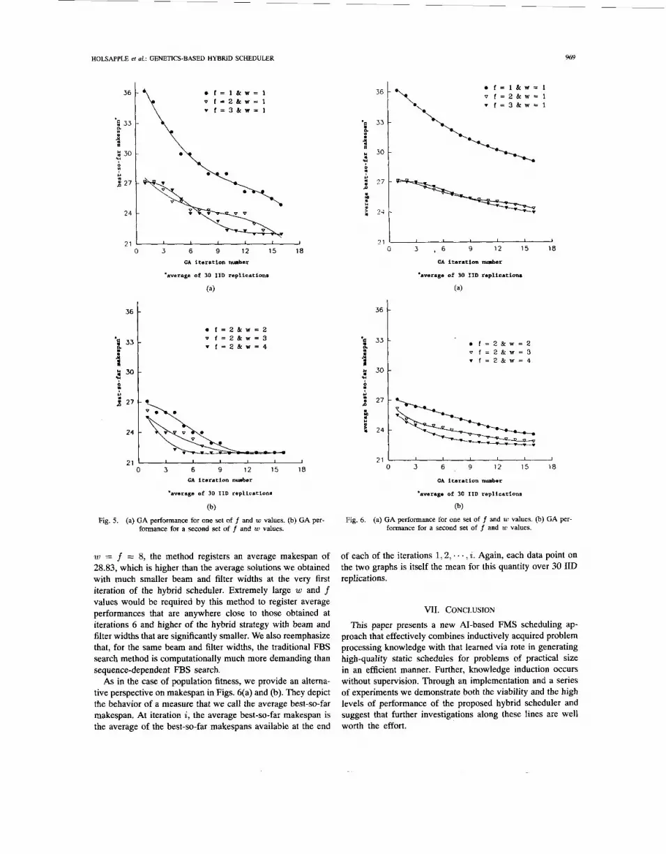
HOLSAPPLE et al.: GENETICS-BASED HYBRID SCHEDULER

. f = l & w = l v f = 2 & w = l T f = 3 & w = l

i"/ 3 \ 2 30 b

1: 27 Y b7

24

21 1 I I I 1 1 J

0 3 6 9 12 15 18 GA iteration number

'average of 30 IID replications

(a)

36

'i 33

4 W

2 30 y: ?

27

24

21

0 f = 2 & w = 2 v f = Z & w = 3 v f = 2 & w = 4

- I I I I I I - .

0 3 6 9 12 15 18 GA iteration number

'average of 30 IID replications

(b) Fig. 5. (a) GA performance for one set of f and w values. (b) GA per-

formance for a second set of f and w values.

w = f = 8, the method registers an average makespan of 28.83, which is higher than the average solutions we obtained with much smaller beam and filter widths at the very first iteration of the hybrid scheduler. Extremely large w and f values would be required by this method to register average performances that are anywhere close to those obtained at iterations 6 and higher of the hybrid strategy with beam and filter widths that are significantly smaller. We also reemphasize that, for the same beam and filter widths, the traditional FBS search method is computationally much more demanding than sequence-dependent FBS search.

As in the case of population fitness, we provide an alterna- tive perspective on makespan in Figs. 6(a) and (b). They depict the behavior of a measure that we call the average best-so-far makespan. At iteration i, the average best-so-far makespan is the average of the best-so-far makespans available at the end

Y

?

36 -

33 -

30 -

S I

969

0 f = l & w = l 0 f = 2 & w = l T f = 3 & w = 1

21 3 I 6 9 12 15 18 0

GA iteration number

*average of 30 IID replicatiow

(a)

36

'5 33

2 30 1 y: W

U a 27

B Y

f 24

21

0 f = 2 & w = 2 v f = 2 & w = 3 T f = 2 & W = 4

I I I I 1 I

3 6 , 9 12 15 18

GA iteration number

*average of 30 IID replications

(b)

formance for a second set of f and w values. Fig. 6. (a) GA performance for one set of f and w values. (b) GA per-

of each of the iterations 1 ,2 , . . . , i. Again, each data point on the two graphs is itself the mean for this quantity over 30 IID replications.

VII. CONCLUSION This paper presents a new AI-based FMS scheduling ap-

proach that effectively combines inductively acquired problem processing knowledge with that learned via rote in generating high-quality static schedules for problems of practical size in an efficient manner. Further, knowledge induction occurs without supervision. Through an implementation and a series of experiments we demonstrate both the viability and the high levels of performance of the proposed hybrid scheduler and suggest that further investigations along these lines are well worth the effort.

970 IEEE TRANSACTIONS ON SYSTEMS, MAN, AND CYBERNETICS, VOL. 23, NO. 4, JULYIAUGUST 1993

In our experiments we held the GA module parameters fixed at “typical” levels. In practice, however, there is no single a priori choice for these values that would apply in all problem instances. We are thus faced with the decision problem of determining appropriate parameter values through analysis or through controlled experimentation, and so forth. We are currently pursuing a strategy wherein an additional “parameter identifier” module attempts to determine appropriate mutation, crossover, and reproduction probabilities dynamically. Further, this extension also considers several different types of muta- tion and crossover operators as opposed to just one of each type. If successful, the approach will alleviate a significant portion of the parameter prespecification problem.

Another issue concerns the kinds of scheduling problems used in our examples and experiments. We have addressed the static FMS scheduling problem here. Efforts are also underway to generalize the proposed approach to efficiently handle the dynamic rescheduling stage of the two-stage scheduling process. Finally, our examples address the single objective sce- nario (i.e., makespan minimization). An important extension would be to address the more complex problem of satisficing multiple scheduling criteria simultaneously.

APPENDIX

Many different variants of the mutation and crossover operators have been suggested in the literature (e.g., see [3], [lo], [20], [21], [22], [52], [63], [64]). Here, we discuss the mechanics of the single-swap mutation and subtour chunking crossover operators.

A. Single-Swap Mutation

Given a parent sequence, F , containing n elements, pick two distinct locations, at random, within the sequence and exchange (i.e., swap) the elements at these locations to create a single offspring sequence, 0. For example, let n = 6 and F = 51, J2, 53, 54, 55, 5 6 . Suppose we randomly select locations 2 and 5. Then, 0 = J1, 5 5 , 5 3 , 54, J2, J6. Single- swap mutation is a special case of the more general k-swap mutation where the swap procedure is repeatedly performed until a total of k swaps, 1 5 k 5 n, is completed.

B. Subtour Chunking Crossover

Given two parent sequences, FI and F2, containing n elements each, an offspring, 0, is constructed from the two parents by alternately taking “chunks” from the two parents and placing them in the offspring sequence at approximately the same positions that they occupied in the parent sequence. Conflicts are resolved by trimming the chunks and sliding them to the nearest available free location.

For example, let n = 6, F1 = 51, 5 2 , 5 3 , 54, 5 5 , 56, and F2 = 5 5 , 54, 51, 5 2 , 56, 5 3 . Randomly select a chunk, say 4 1 , 5 2 , 53>, from F1. This chunk begins at location 1 in F1 and we place it at the same location in 0, as this location is unoccupied. Hence, the first three elements in 0 are 51, 5 2 , and 53. Next, randomly select a chunk, say 4 5 , J4, 5 1 , J2> from Fz. Trim the chunk down to <J5, 54> to avoid duplication of 51 and 5 2 in the offspring. The trimmed chunk begins at location 1 in F2. As position 1 in 0 is already occupied we

slide the new chunk over to the next available free space that is closest to position 1. This location is position 4 which is to the right of position 1, the ideal location. Thus, 55 and 54 occupy, respectively, positions 4 and 5 in 0. We repeat the process, alternating between FI and F2 until all locations in 0 become filled. Suppose chunk <J5, J6> is selected next from F1. We trim the chunk down to <&> to avoid duplication. The trimmed chunk begins at location 6 in Fl. As location 6 in 0 is free, we place 56 in this slot. The process terminates as all available positions in 0 are now filled. The offspring generated is 0 = J1,J2 , J3, J5, J4, Js .

ACKNOWLEDGMENT

The authors would like to thank the three anonymous referees and the editor for their invaluable suggestions for improving this paper.

REFERENCES

J. C. Ammons, C. B. Lofren, and L. F. McGinnis, “A large scale work- station loading problem,” Ann. Operations Res., vol. 3, pp. 319-332, 1985. J. M. Bastos, “Batching and routing: two functions in the operational planning of flexible manufacturing systems,” Eur. J. Operational Res., vol. 33, pp. 230-244, 1988. R. K. Belew and L. B. Booker, Eds., Proc. Fourth Int. Conf: Genetic Algorithms. San Mateo, CA: Morgan Kaufmann, 1991. M. Berrada and K. E. Stecke, “A branch and bound approach for machine loading in flexible manufacturing systems,” Management Sci., vol. 32, pp. 1316-1335, 1986. L. B. Booker, D. E. Goldberg, and J. H. Holland, “Classifier systems and genetic algorithms,” Artificial Intell., vol. 40, pp. 235-282, 1989. G. Bruno, A. Elia, and P. Laface, “A rule-based system to schedule production,” IEEE Comput., pp. 32-39, July 1986. W. I. Bullers, S. Y. Nof, and A. B. Whinston, “Artificial intelligence in manufacturing planning and control,” HIE Trans., pp. 351-363, Dec. 1980. J. G. Carbonell, R. S. Michalski, and T. M. Mitchell, “An overview of machine learning,” in Machine Learning: An Artificial Intelligence Approach, vol. 1, R. S. Michalski, J. G. Carbonell, and T. M. Mitchell, Eds. Y. L. Chang, R. S. Sullivan, U. Bagchi, and J. R. Wilson, “Experimental investigation of real-time scheduling in flexible manufacturing systems,” Ann. Operations Res., vol. 3, pp. 355-378, 1985. G. A. Cleveland and S. F. Smith, “Using genetic algorithms to schedule flow shop releases,” in Proc. Third Int. Conf: Genetic Algorithms, D. Schaffer, Ed. W. G. Cochran, Sampling Techniques. P. R. Cohen and E. A. Feigenbaum, The Handbook of Artificial Intelli- gence, vol. 3. W. J. Davis and A. T. Jones, “A real-time production scheduler for a stochastic manufacturing environment,” Int. J . Computer Integrated Manufacturing, vol. 1, pp. 101-112, 1988. S. De, “A knowledge-based approach to scheduling in an FMS,” Ann. Operations Res., vol. 12, pp. 109-134, 1988. S. De and A. Lee, “Flexible manufacturing system (FMS) scheduling using filtered beam search,” J. Intelligent Manufacturing, vol. 1, pp. 165-183, 1990. M. S. Fox, Constraint-Directed Search: A Case Study of Job Shop Scheduling. San Mateo, CA: Morgan Kaufmann, 1987. M. S. Fox and S. F. Smith, “ISIS: a knowledge-based system for factory scheduling,” Expert Syst., vol. 1, pp. 2 5 4 9 , 1984. F. Glover, “Tabu search - part I,” ORSA J. Computing, vol. 1, pp. 190-206, 1989. F. Glover, “Tabu search - part 11,” ORSA J. Computing, vol. 2, pp. 4-32, 1990. D. E. Goldberg, Genetic Algorithms in Search, Optimization and Ma- chine Learning. J. J. Grefenstette, Ed., in Proc. Int. Conf: Genetic Algorithms and Their Applications. Hillsdale, NJ: Lawrence Erlbaum Associates, 1985. -, Genetic Algorithms and Their Applications: Proc. Second Int. Conf: Genetic Algorithms. Hillsdale, NJ: Lawrence Erlbaum Asso- ciates, 1987.

San Mateo, CA: Morgan Kaufmann, 1983.

San Mateo, CA: Morgan Kaufmann, 1989. New York: Wiley, 1977.

San Mateo, CA: Morgan Kaufmann, 1982.

Reading, MA: Addison Wesley, 1989.

HOLSAF’PLE et al.: GENETICS-BASED HYBRID SCHEDULER 971

[23] M. R. Hilliard, G. E. Liepins, M. Palmer, M. Morrow, and J. Richardson “A classifier-based system for discovering scheduling heuristics,” in Genetic Algorithms and Their Applications: Proc. Second Int. Conf Genetic Algorithms, J. J. Grefenstette, Ed. Hillsdale, NJ: Lawrence Erlbaum Associates, 1987.

[24] M. R. Hilliard, G. E. Liepins, M. Palmer, and G. Rangarajan, “The computer as a partner in algorithmic design: automated discovery of parameters for a multi-objective scheduling heuristic,” in Impacts of Recent Computer Advances on Operations Research R. Sharda, B. Golden, E. Wasil, 0. Balci, and W. Stewart, Eds. New York: North Holland, 1989.

[25] M. R. Hilliard, G. E. Liepins, G. Rangarajan, and M. Palmer, “Learning decision rules for scheduling problems: a classifier hybrid approach,” in Proc. Sixth Int. Conf Machine LearninR. San Mateo, CA: Morgan Kaufmann, 1989.

1261 K. L. Hitz, “Scheduling in flexible flow shops I,” Tech. Rep. No. 879, L 1

Laboratory for 1nforma;ion and Decision Syitems, Mass. Inst. Technol, Cambridge, MA, 1979.

[27] J. H. Holland, Adaptation in Natural and Artificial Systems. Ann Arbor, MI: The University of Michigan Press, 1975.

[28] J. H. Holland, K. J. Holyoak, R. E. Nisbett, and P. R. Thagard,Induction: Processes of Inference, Learning, and Discovery. Cambridge, MA: The MIT Press, 1986.

[29] C. W. Holsapple, V. S. Jacob, R. Pakath, and J. S. Zaveri, “Learning by problem processors: adaptive decision support systems,” Decision Support Syst., vol. 10, pp. 85-108, 1992.

[30] E. Horowitz and S. Sahni, “Computing partitions with application to the knapsack problem,” J . ACM, vol. 21, pp. 277-292, 1974.

[31] M. S. Hung and J. C. Fisk, “An algorithm for 0-1 multiple knapsack problems,” Naval Res. Logistics Quart., vol. 2.5, pp. 571-579, 1978.

[32] G. K. Hutchinson, “The control of flexible manufacturing systems: required information and control structures,” in Proc. IFAC Symp. Information-Control Problems in Manufacturing Technology, Tokyo, Japan: 1977.

[33] V. S. Jacob, R. Pakath, and J. S. Zaveri, “Adaptive decision support systems: incorporating learning into decision support systems,” in Proc. 1990 ISDSS Conf. Austin, TX: IC2 Institute, The University of Texas at Austin, 1990.

[34] A. H. G. R. Kan, Machine Scheduling Problems. The Hague, The Netherlands: Martinus Nijhoff, 1976.

[35] J. J. Kanet and H. H. Adelsberger, “Expert systems in production scheduling,” Eur. J. Operational Res., vol. 29, pp. 51-57, 1987.

[36] J. G. Kimemia and S. B. Gershwin, “An algorithm for the computer control of a flexible manufacturing system,” IIE Trans., vol. 15, pp. 353-363, 1983.

[37] S. Kirkpatrick, C. D. Gelatt Jr., and M. P. Vecchi, “Optimization by simulated annealing,” Science, vol. 220, pp. 671-674, 1983.

[38] Y. Kodratoff and R. Michalski, Machine Learning: An Artificial Intelli- gence Approach, vol. 3.

[39] A. Kusiak, “Designing expert systems for scheduling of automated manufacturing,” Industrial Engineering, vol. 19, pp. 4 2 4 6 , 1987.

[40] A. Kusiak and M. Chen, “Expert systems for planning and scheduling manufacturing systems,” Eur. J. Operational Res., vol. 34, pp. 113-130, 1988.

(411 R. J. Mayer and J. J. Talvage, “Simulation of computerized manufac- turing systems,” Rep. No. 4, NSF Grant No. APR 74-15256, 1976.

[42] R. S. Michalski, “Understanding the nature of learning: issues and research directions,” in Machine Learning: An Artificial Intelligence Approach, vol. 2, R. S. Michalski, J. G. Carbonell, and T. M. Mitchell, Eds.

[43] R. S. Michalski, J. G. Carbonell, and T. M. Mitchell, Machine Learning: An Artificial Intelligence Approach, vol. 1. San Mateo, CA: Morgan Kaufmann, 1983.

1441 R. S. Michalski. J. G. Carbonell. and T. M. Mitchell. MachineLearninp:

San Mateo, CA: Morgan Kaufmann, 1990.

San Mateo, C A Morgan Kaufmann, 1986.

[451

An Artificial Intelligence Approach, vol. 2. San Mateo, CA: Morgan Kaufmann, 1986. R. S. Michalski and Y. Kodratoff, “Research in machine learning: recent progress, classification of methods, and future directions,” in Machine Learning: An Artificial Intelligence Approach, vol. 3, Y. Kodratoff and R. S. Michalski, Eds. T. L. Morin and R. E. Marsten, “An algorithm for non-linear knapsack problems,” Management Sci., vol. 22, pp. 1147-1 158, 1976. G. J. Olsder and R. Suri, “Time optimal control of parts from routing in a manufacturing system with failure prone machines,” in Proc. 19th IEEE Conf. Decision and Contr.. Albuquerque, NM, 1980. P. S. Ow and T. E. Morton, “Filtered beam search in scheduling,” Int. J. Production Res., vol. 26, pp. 35-62, 1988. P. S. Ow, S. F. Smith, and R. Howie, “A cooperative scheduling

San Mateo, CA: Morgan Kaufmann, 1490.

system,” in Expert Systems in Intelligent Manufacturing, M. D. Oliff, Ed. Amsterdam: North Holland, 1988.

[SO] V. Raghavan, “An expert system framework for the management of due dates in flexible manufacturing systems,” in Expert Systems in Intelligent Manufacturing, M. D. Oliff, Ed.

(511 S. Rajagopalan, “Formulation and heuristic solutions for parts grouping and tool loading in flexible manufacturing systems,” in Proc. Second ORSAITIMS Conf Flexible Manufacturing Systems, 1986.

152) J. D. Schaffer, Proc. Third fnt. Conf: Genetic Algorithms. San Mateo, CA: Morgan Kaufmann, 1989.

[53] K. Shanker and Y. J. J. Tzen, “A loading and despatching problem in a random flexible manufacturing system,” Int. J. Production Res., vol. 23, pp. 579-595, 1985.

[54] J. G. Shanthikumar and R. G. Sargent, “A hybrid simulationlanalytic model of a computerized manufacturing system,” Working Paper No. 8 M 1 7 , Syracuse Univ., Syracuse, NY, 1980.

(551 J. W. Shavlik and T. G. Dietterich, Readingsin MachineLearning. San Mateo, CA: Morgan Kaufmann, 1990.

[56] M. J. Shaw, “Knowledge-based scheduling in flexible manufactur- ing systems: an integration of pattern-directed inference and heuristic search,” Int. J. Production Res., vol. 26, pp. 821-844, 1988.

[57] M. J. Shaw, “A pattern-directed approach to FMS scheduling,” Ann. Operations Res., vol. 15, pp. 353-376, 1988.

[58] M. J. Shaw, S. C. Park, and N. Raman, “Intelligent scheduling with machine learning capabilities: the induction of scheduling knowledge,” IIE Trans., vol. 24, pp. 156-168, 1992.

[59] M. J. Shaw and A. B. Whinston, “An artificial intelligence approach to the scheduling of flexible manufacturing systems,” IIE Trans., vol. 21, pp. 170-183, 1989.

[60] S. Shen and Y. Chang, “Schedule generation in a flexible manufacturing svstem: a knowledge-based approach,” Decision Support Systems, vol.

Amsterdam: North Holland, 1988.

.. .- . 4 pp. 157-166, 1688. 1611 K. E. Stecke and F. B. Talbot, “Heuristics for loading flexible manu- > >

facturing systems,” in Flexible Manufacturing Systems: Recent Devel- opments in FMS, CADICAM, CIM, A. Raouf and S. 1. Ahmad, Eds, 1985.

[62] S. Subramanyam and R. G. Askin, “An expert systems approach to scheduling in flexible manufacturing systems,” in Flexible Manufactur- ing Systems: Methods and Studies, A. Kusiak, Ed. Amsterdam: North Holland, 1986.

[63] G. Syswerda, “Schedule optimization using genetic algorithms,” Work- ing Paper, BBN Laboratories, BBN Systems and Technologies Corp. , Cambridge, MA, 1990.

1641 D. Whitley, T. Starkweather, and D. Fuquay, “Scheduling problems and traveling salesmen: The genetic edge recombination operator,” in Proc. Third Int. Conf Genetic Algorithms, D. Schaffer, Ed. San Mateo, CA: Morgan Kaufmann, 1989.

[65] C. K. Whitney and T. S. Goul, “Sequential decision procedures for batching and balancing in FMS’s.” Ann. Operations Res., vol. 3, pp. - ..

301-3116, 1985. [66] P. H. Winston, Artificial Intelligence. Reading, MA: Addison-Wesley,

1984. [67] S. D. Wu and R. A. Wysk, “An application of discrete-event simulation

to on-line control and scheduling in flexible manufacturing,” Int. J . Production Res., vol. 27, pp. 1603-1623, 1989.

[68] R. A. Wysk, S. D. Wu, and N. Yang, “A multi-pass expert control system for manufacturing systems,” in Proc. Symp. Real-time Optimization in Automated Manufacturing Facilities. Gaithersburg, MD: National Bureau of Standards, 1986.

Sciences, IEEE Expert, and Management, Exp

Clyde W. Holsapple received the doctorate in man- agement science from Purdue University in 1977.

He is Professor of Decision Science and Infor- mation Systems and holds the Rosenthal Endowed Chair in Management Information Systems at the University of Kentucky. In addition to his books in the decision support system, data base man- agement, and expert system areas, he has many research articles published in such journals as De- cision Support Systems, Operations Research, The Computer Journal, Organization Science, Decision

Financial Management, Policy Sciences, Information nrt Systems, and Information Systems.

972 IEEE TRANSACTIONS ON SYSTEMS, MAN, AND CYBERNETICS, VOL. 23, NO. 4, JULYIAUGUST 1993

Dr. Holsapple has served Area Editor for Decision Support Systems and ORSA Journal on Computing. He is Associate Editor for Organizational Computing and Management Science. In 1993, he was recognized as “Com- puter Educator of the Year” by the International Association for Computer Information Systems.

Varghese S. Jacob (S’85-M’86) received the Ph.D. degree in management in 1986 from Purdue University, West Lafayette, IN.

He is an Associate Professor of Management Information Systems at The Ohio State University. His research interests are in decision support systems, expert systems, distributed systems, and machine learning.

Dr. Jacob has published articles in various journals including Decision Support Systems, IEEE TRANSACTIONS ON SYSTEMS, MAN, AND

CYBERNETICS, Journal of Economic Dynamics and Control, and International Journal of Man-Machine Studies.

Dr. Jacob is a member of the Institute of Management Science, IEEE Computer Society, Association of Computing Machinery and American Association of Artificial Intelligence.

Ramakrishnan Pakath received the Ph.D. degree in management (MIS) in 1988 from the Krannert Graduate School of Management, Purdue Univer- sity, West Lafayette, IN.

He is an Associate Professor of Decision Sci- ence and Information Systems at the University of Kentucky. His research interests and experience are primarily in the design and implementation of systems incorporating AI-based processing meth- ods, conventional algorithmic processing methods, or hybrid AI-based-conventional algorithmic pro-

cessing methods for centralized and distributed decision support. A closely

related subtheme of his research is the assessment of information value in decision modeling. His articles have appeared in such forums as Behaviour and Information Technology, Computer Science in Economics and Manage- ment, Decision Support Systems, European Journal of Operational Research, Handbook of Industrial Engineering, IEEE TRANSACTIONS ON SYSTEMS, MAN, AND CYBERNETICS, Information and Management, and Journal of Computer Information Systems.

Dr. Pakath is an Associate Editor for Decision Support Systems and is the Acting Director of the MIS and DSS Research Laboratories at the University of Kentucky.

Jigish S. Zaveri received the B.Tech. degree in chemical engineering in 1985 from the Indian Insti- tute of Technology, Kharagpur, India, and the M.S. degree in chemical engineering and the Ph.D. degree in business administration in 1988 and 1992 from the University of Kentucky, Lexington.

He is Assistant Professor of Information Systems at Morgan State University, Baltimore, MD. His teaching and research interests encompass decision support systems, expert systems, machine learning, and manufacturing. His articles have appeared in

Decision Support Systems and IEEE TRANSACTIONS ON SYSTEMS, MAN, AND CYBERNETICS.

Dr. Zaveri is a member of the Decision Sciences Institute and the Production and Operations Management Society.