Synthesis and stochastic assessment of cost-optimal schedules

Synthesis and Stochastic Assessment of Cost-OptimalSchedulesAngelika Mader1, Henrik Bohnenkamp2, Yaroslav S. Usenko3,David N. Jansen1, Johann Hurink1, Holger Hermanns4,1

1 University of TwenteFaculty EWI, 7500 AE Enschede, The Netherlandse-mail: {a.h.mader|david.n.jansen|j.l.hurink}@utwente.nl

2 RWTH Aachen UniversityModeling and Verification of Software Group (MOVES), Info 2, 52056 Aachen, Germanye-mail: [email protected]

3 Technical University of EindhovenLaboratory for Quality Software (LaQuSo), 5600 MB Eindhoven, The Netherlandse-mail: [email protected]

4 Saarland UniversityDependable Systems and Software Group, 66041 Saarbrucken, Germanye-mail: [email protected]

Abstract We present a novel approach to synthesize good schedules for a classof scheduling problems that is slightly more general than the scheduling prob-lem FJm, a|gpr, rj, dj |early/tardy. The idea is to prime the schedule synthesizerwith stochastic information more meaningful than performance factors with theobjective to minimize the expected cost caused by storage or delay. The priminginformation is obtained by stochastic simulation of the system environment. Thegenerated schedules are assessed again by simulation. The approach is demon-strated by means of a non-trivial scheduling problem from lacquer production. Theexperimental results show that our approach achieves in all considered scenariosbetter results than the extended processing times approach.

Key words Schedule synthesis – Stochastic – Resource Failures – Heuristics

1 Introduction

In this paper we deal with a scheduling problem where the resources are prone tofailures. The stochastic nature of machine breakdowns makes the problem hard totackle and, in practice, they cannot only cause delays that were not anticipated, butcan devaluate the whole schedule. Looking at the current literature on scheduling(see e. g., [25] for an overview) one observes that stochastic effects are hardly taken

2 A. Mader et al.

into account. Only for simple models (mainly single machine models) methodsexists to deal explicitely with stochastic influences on the data. A common way toget rid of the uncertainty is to abstract to expected values and to incorporate slackor margins into the data.

A possible realization of this approach for stochastic machine breakdowns is todefine so called performance factors, which describe the ratio p = uptime/(uptime+downtime) of a resource. The approach to account for failures then extends theprocessing times of tasks by a factor of 1/p. These extended processing times(EPT) are then used to generate deterministic schedules.

This approach has a justification, if acceptable production load on the long termhas to be investigated.A different, relevant question is, however, how this approachworks if orders have to be finished at a certain due date. It is possible to generateschedules with extended processing times, which do meet the due date, but thequestion is to what extent these schedules hold up in a realistic environment,whereresources do fail.

We will investigate this problem by means of a case study that was proposed inthe context of the meanwhile finished IST project AMETIST (AdvancedMethodsfor Timed Systems) [3]. The case study was suggested by the industrial partnerAxxom, a company that provides planning and logistics solutions. This case studyis about schedule generation for lacquer production. Lacquers are produced ac-cording to certain recipes, which are sub-divided into tasks. The execution of tasksrequires resources, which are prone to failures. The failure behaviour is describedby performance factors. Three types of recipes are considered: metal, uni, andbronce. Each order is specified by a lacquer type and a due date. In the frameworkof the case study, a fixed set of 29 orders is used.We use this case study as a vehicleto demonstrate our approach.

In a previous paper [10], we have investigated schedules in the lacquer pro-duction framework with respect to feasibility, i. e., whether orders are finished be-fore their due dates. The schedules are synthesized using the model checker UP-PAAL [26], both for net and extended processing times. In a real production settingwith stochastic elements, deterministic schedules can not be followed completely,in general. Therefore, we focus on the starting times of orders, and regard them asthe most relevant element of a schedule. We assess the schedules by simulation,making reasonable assumptions about the failure behaviour of resources.We createa simulation model of the lacquer production plant using the modelling languageMODEST [12], and simulate the 29 orders according to the generated schedulewith the simulator of the performance tool M OBIUS [16,18,11]. The quintessenceof this study is that schedules generated with extended processing time have morechance to miss the due date than schedules based on net processing times. This canbe explained by observing that in the EPT approach time is reserved for machinefailure, even in the case the machine is up. If the machine goes down later, notenough time is left to repair it and finish in time.

The original question of the case study as proposed by Axxom, however, wasnot focussing on feasibility, but on schedules that minimize an objective function.Following these lines we include costs for each order missing its due date. Thereare two types of cost: storage costs, which are incurred when an order is finished

Synthesis and Stochastic Assessment of Cost-Optimal Schedules 3

before the due date, and delay costs, which are incurred if an order is finished afterthe due date. We consider again the scenario of 29 orders as described before, withthe difference that every order has not only a due date, but also a storage cost factorand a delay cost factor attached. As before, resources are prone to failure.

Our research question here is how to synthesize schedules that minimize costsin a setting where resources can fail. More precisely, we suggest a new approachand evaluate it against the EPT appraoch. Technically, we synthesize different setsof schedules, for one part following the EPT approach, for the other part followingour suggested method, and assess all by stochastic simulation.

The first set of schedules we generate is based on net and EPT processingtimes, respectively. The tool we use is the model-checker UPPAAL CORA, a ver-sion of UPPAAL which allows to attach costs to states of the considered modeland which allows to find schedules that minimize the costs. The principles of thisapproach have been described in several publications [8,5,6].

The second set of schedules is generated according to our new approach. Weproceed in two steps: first, for each individual order we determine a quantity whichwe call the optimal starting time (OST). Second, we synthesize schedules wherethe effective starting times of orders are as close as possible to their respectiveOSTs.

OSTs are determined in a way that starting an order at its OST minimizes theexpected cost. Note that the OSTs are not chosen such that the mean completiontime of an order is its due date, which constitutes the main difference to the EPTapproach. We derive the OSTs by simulating the different recipes and determinethe run-time distribution for each order type. UPPAAL CORA is used to generateschedules with effective starting times of orders as close as possible to the re-spective OSTs. Due to resource conflicts orders might not be able to start at theirprecomputed OSTs. The synthesized schedule contains information about start-ing times of all tasks and orders, but we regard the release times of orders in theproduction process as the only relevant information.

As in [10], we assess the quality of the schedules by simulation, making rea-sonable, more detailed assumptions about the failure behaviour of the resources.Our measure of interest, for the EPT- as well as for the OST-based schedules, isthe mean total cost that is incurred by executing all 29 orders according to theschedule.

Our experiments show that the OST based schedules indeed effectuate lessexpected costs than the EPT based schedules. Schedules based on net processingtimes give highest costs. Additionally, it turns out that our approach is also robustagainst erroneous assumptions on the failure distribution: even if the failure dis-tribution as basis for the OSTs differs from the failure distribution chosen in thesimulation, the cost is not higher than for the EPT approach, and in most casessignificantly better. Apart from the result that our suggested approach works, theexperiments also show that there is room for more fine-tuning of the OSTs, whichgives rise to future research.

While we demonstrate our approach on this particular example, it is worth tohighlight, that it generalizes to a whole range of settings. Furthermore, the toolswe use, UPPAAL CORA and MOBIUS could, in principle, be substituted by other

4 A. Mader et al.

tools. For us, the flexibility in modelling different settings, and the capability todeal with our questions, made them comfortable to use.Organisation of the paper: The lacquer-production case study we use to

demonstrate our approach is introduced in Section 2. In Section 3, we presentthe tools to generate and simulate schedules. In Section 4 we explain our OSTapproach in detail. Experiments and their results are collected in Section 5. Weconclude with Section 6.

2 Lacquer Production Case

The purpose of this section is to present the necessary details of the lacqer-produc-tion case study, which has a non-trivial scheduling problem with several complexaspects. Research on this case-study has led to several publications [10,24,5,6].

We start with a short description of the case and continue with its classificationfollowing the standard scheme for machine scheduling problems [19].

There are three recipes for different types of lacquer: metallic, bronce and unilacquers. Each recipe describes the processing steps, their durations, their interde-pendency, precedence relations with timing constraints, and finally, the resourcesto use. A recipe is composed of tasks. Each task describes which resource it re-quires, and for how long that resource is needed. The latter time value is calledthe processing time of the task. Figure 1 contains a graphical representation of thethree considered recipes. The rectangular objects represent the tasks. The patternsindicate the resource type needed to execute the task, and the numbers the process-ing time in minutes. The tasks related to mixing vessels are implicit, since they donot have prespecified processing times but last as long as the parallel tasks are per-formed. Vertical lines denote dependencies between the tasks (top to bottom), andhorizontal lines represent synchronisation. In the case no numbers are given nextto the vertical lines, the dependencies express ordinary precedence constraints be-tween the tasks, indicating that the later task may only start its processing after theformer task has finished. If an interval [a, b] is given next to the vertical line, thisindicates that the later task has to start later than the preceding task by an amountin range between a and b.

An order of a certain type of lacquer is specified by the type of lacquer to beproduced and the earliest possible starting time and the due date until which ithas to be finished. An order that is finished before the due date will cause storagecosts, finishing after the due date causes delay costs. Axxom assumes that costs areincurred linearly with time, i. e., the storage cost and delay cost can be describedby a piecewise linear function with two parameters scf and dcf : the storage costfactor and the delay cost factor.As a result, the costs c(d, t) of finishing a job withdue date d at time t is given by

c(d, t) ={

scf(d ! t) if t " ddcf(t ! d) if t > d.

Figure 2 contains a schematic representation of the cost function with respect tothe due date. An order finished precisely at the due date will cause zero costs.


metallic bronce uni

mixing vessel metal

dose spinner

laboratory

lling station

bronce mixer

dose spinner bronce

disperging line

disperser

waitarbitrarily, unless speciedsynchronize

mixing vessel uni

[240,240]

1058

311

441

395

1323

1058

311

441

1664

1323

[360,360] 705 353

[0,240]

662

311

441

1437

1542

[360,360]

2939

1587

[240,240][240,240]

Fig. 1 Lacquer recipes indicating the resources needed, durations of processing steps andprecedence relations with timing constraints

due datetime

cost

Fig. 2 Cost function for product finish time

6 A. Mader et al.

order type due scf dcf

1 metal 27444 8 4292 metal 33348 8 3903 metal 33636 11 5744 metal 36372 8 4255 metal 37092 10 4966 metal 40500 11 5847 metal 41699 15 7798 metal 47172 10 5319 metal 56964 10 49210 metal 57252 14 70811 metal 57539 14 69112 metal 62148 7 36813 metal 67764 6 28314 metal 67980 7 35415 metal 71868 4 213

order type due scf dcf

16 bronce 43500 17 917 bronce 50580 15 74418 bronce 60660 10 53119 bronce 61859 13 67320 bronce 65100 8 421 uni 30459 3 17722 uni 41628 3 223 uni 43764 7 35424 uni 44004 6 28325 uni 50580 10 53126 uni 60588 7 427 uni 61788 10 528 uni 77124 8 39029 uni 85764 8 425

Table 1 The parameters for the 29 considered orders

In the case study, a fixed set of 29 orders is given, each described by a lacquertype, a due date, and respective scf and dcf . In Table 1, we summarize the parame-ters for the different orders. Note that for most orders, scf < dcf , and the relationdcf /scf is in the order of 30 to 60. This observation will become important inSection 4. However, for some few orders, scf > dcf holds.

As can be seen in Figure 1, there are nine different types of resources. Re-sources are subject to failure, and the failure behaviour of resource type r is de-scribed by a performance factor pr. Intuitively, the performance factor is the ratioof uptime/(uptime + downtime), where uptime and downtime are the up- anddowntime of the resource. The values uptime and downtimemust actually be con-sidered as random variables, since the failure of a resource is a stochastic phe-nomenon. However, no information was available about the mean durations of up-and downtime, or even the distributions.

To get a clear understanding of the problem, we classify the lacquer productionscenario in the project scheduling terminology (see e. g., [19]). The consideredproblem is a slight generalization of the problem FJm, a|gpr, r j, dj |early/tardy.Here

– ’α = FJm, a’ specifies the resource characteristics as a flexible job-shopproblem, where– each order has to follow its own route,– a fixed number of m resource types are given with a given number of in-stances per type. In the concrete case 9 resource types with the followinginstances per resource types are given:


pr 0.85 0.75 1.0

r

Dose SpinnerLaboratoryFilling Station

Bronce MixerDose Spinner BronceDisperging LineDisperser

Mixing Vessel UniMixing Vessel Metal

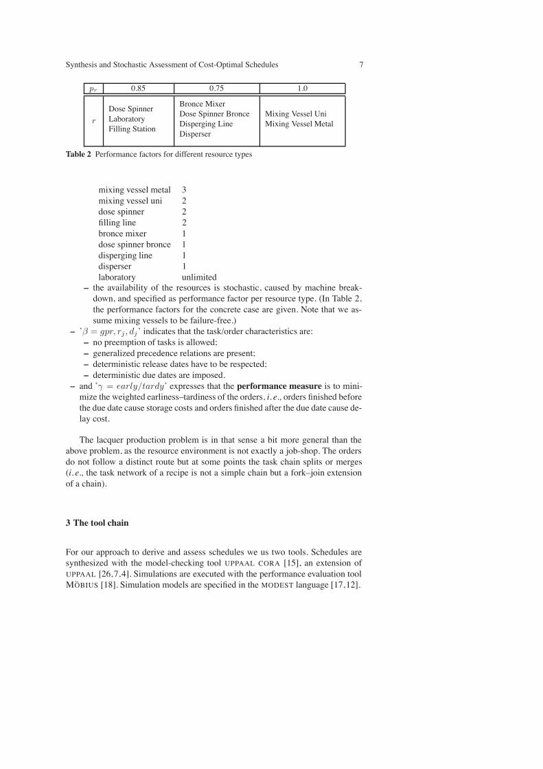
Table 2 Performance factors for different resource types

mixing vessel metal 3mixing vessel uni 2dose spinner 2filling line 2bronce mixer 1dose spinner bronce 1disperging line 1disperser 1laboratory unlimited

– the availability of the resources is stochastic, caused by machine break-down, and specified as performance factor per resource type. (In Table 2,the performance factors for the concrete case are given. Note that we as-sume mixing vessels to be failure-free.)

– ’β = gpr, rj , dj’ indicates that the task/order characteristics are:– no preemption of tasks is allowed;– generalized precedence relations are present;– deterministic release dates have to be respected;– deterministic due dates are imposed.

– and ’γ = early/tardy’ expresses that the performance measure is to mini-mize the weighted earliness–tardiness of the orders, i. e., orders finished beforethe due date cause storage costs and orders finished after the due date cause de-lay cost.

The lacquer production problem is in that sense a bit more general than theabove problem, as the resource environment is not exactly a job-shop. The ordersdo not follow a distinct route but at some points the task chain splits or merges(i. e., the task network of a recipe is not a simple chain but a fork–join extensionof a chain).

3 The tool chain

For our approach to derive and assess schedules we us two tools. Schedules aresynthesized with the model-checking tool UPPAAL CORA [15], an extension ofUPPAAL [26,7,4]. Simulations are executed with the performance evaluation toolMOBIUS [18]. Simulation models are specified in the MODEST language [17,12].

8 A. Mader et al.

3.1 UPPAAL and UPPAAL CORA

Automata are a well-known description model for concurrent systems. Timed au-tomata [1] are an extension of finite-state automata with real time clocks. Clockscan be reset, used in guards on transitions and in invariants on locations.

UPPAAL is an integrated tool environment for modeling, validation and modelchecking of real-time systems modelled as networks of timed automata, extendedwith data types (bounded integers, arrays, etc.). The tool was developed in collab-oration between the Department of Information Technology at Uppsala University,Sweden and the Department of Computer Science at Aalborg University in Den-mark.

Model checking [14,22] is an advanced method to formally verify concurrentfinite-state systems. Specifications about the system are expressed as temporallogic formulas, and efficient symbolic algorithms are used to traverse the modeldefined by the system and check if the specification holds or not. Extremely largestate-spaces can often be traversed within minutes.

UPPAAL CORA [15] is a branch of UPPAAL for Cost Optimal ReachabilityAnalysis. Whereas UPPAAL supports model checking of timed automata, UPPAALCORA uses an extension of timed automata called linear priced timed automata(LPTA) [9,2]. LPTA allows to annotate the model with the notion of cost. Costscan be defined for delay while staying in a location, or costs for a particular action.UPPAAL CORA then finds optimal paths matching goal conditions.

Scheduling synthesis by model checking works along the following lines: As-sume we have a model of the uncontrolled production process. The model checkersearches for a state with the property all orders are finished. Once it has foundsuch a state the model checker can provide a diagnostic trace, i. e., a trace fromthe initial state to the state with the desired property. This trace contains all theinfomation on start and finish (times) of production steps, as well as informationabout resources, and, in the context of scheduling, represents a valid schedule.

This technique can also be applied to linear priced timed automata. Here, themodel checker searches for the cheapest state having the desired property. Havingfound such a state, the diagnostic trace then provides a cost-optimal schedule. Inpractice we have to deal with very large state spaces and we can not expect tofind a cheapest state, resp. an optimal schedule. However, it was shown that thistechnique, extended by suitable heuristics, allows to find good schedules in veryshort time [5,6].

What makes the timed automaton environment attractive for solving schedul-ing problems is the robustness against variations in the parameter setting. By thiswe mean that timed automata are a general description language and allow for anenormous variation in problem descriptions: it is easy to change, add, or removemodel parameters without changing the search mechanism. On the other hand,this advantage comes for the price of state-space explosion, which, however, canbe handled by suitable heuristics.


3.2 MODEST and MOBIUS

MODEST is a formal language to describe stochastic timed systems [17,12], equip-ped with a rigid formal semantics. The functional core of MODEST can be consid-ered as a simple process algebra enriched with some convenient language con-structs. The syntax resembles that of the programming language C and the model-ing language Promela [21]. Data modularization concepts and exception handlingmechanisms have been adopted from modern object-oriented programming lan-guages such as Java. Process algebraic constructs have been strongly influencedby FSP (Finite State Processes [23]), a simple, elegant calculus that is aimed ateducational purposes.

This core language is enriched with several modeling concepts tailored tomodel timed and stochastic systems. We highlight three particular semantic con-cepts which are well-established in the context of real-time and stochastic discreteevent systems:

– Probabilistic branching is a way to include quantitative information about thelikelihood of choice alternatives.

– Clocks are a means to represent real time and to specify the dynamics of amodel in relation to a certain time or time interval, represented by a specificvalue of a clock.

– Random variables are often used to give quantitative information about thelikelihood of a certain event to happen after or within a certain time interval.

The MODEST language allows one to specify processes, and to compose them inparallel using a parallel composition operator. Processes can manipulate data vari-ables by assignments. Data variables are typed and must be declared, and the pointof declaration determines their scope. In particular, they may be local to a process,or global, in which case they are shared between all processes. A particular typeof variable which can be declared is the clock type. Clocks can be read like anordinary float variable, but advance their value linearly to the real-valued simula-tion time. All clocks run at the same speed. Clocks can only be set to zero. Thelanguage provides generic constructs to sample values from a set of predefinedprobability distributions. For instance, ‘xd = Uniform(10, 20)’ assigns a samplefrom the uniform distribution on the interval [10, 20] to the variable ‘xd’. Othertypes of distributions are, e. g., Exponential(rate) and Normal(mean,var).

Apart from manipulating data, processes can interact with other parallel pro-cesses (or the environment) bymeans of actions. Their occurrencewithin a processcan be guarded by a ‘when’ clause, specifying an enabledness condition. In partic-ular, the boolean expression in a ‘when’ clause may refer to clock values. In thatcase, an action may be enabled as soon as the when condition becomes true (andno other action becomes enabled earlier). We assume a maximal progress seman-tics, which means that an actions is taken as soon as it is enabled, i. e., idling haslower priority that performing actions.

10 A. Mader et al.

MOBIUS is a performance evaluation tool environment1. MOBIUS supportsmultiple input formalisms and several evaluation approaches for these models.Atomic models are specified in one of the available input formalisms. Atomicmodels can be composed by means of state-variable sharing, yielding so-calledcomposed models. Notably, atomic models specified in different formalisms canbe composed in this way. This allows to specify different aspects of a system underevaluation in the most suitable formalism. Along with an atomic or composedmodel, the user specifies a reward model, which defines a reward structure on theoverall model. Note that rewards are the vehicle to define the costs for our casestudy.

On top of a reward model, the tool provides support to define experiment se-ries, called Studies, in which the user defines the set of input parameters for whichthe composed model should be evaluated. Each combination of input parametersdefines a so-called experiment. Before analyzing the model experiments, a solutionmethod has to be selected: MOBIUS offers a powerful (distributed) discrete-eventsimulator, and, for Markovian models, explicit state-space generators and numeri-cal solution algorithms. It is possible to analyze transient and steady-state rewardmodels. The solver solves each experiment as specified in the Study. Results canbe administered by means of a database.

MOTOR. In order to facilitate the analysis of MODEST models, we have devel-oped the prototype tool MOTOR [13]. The philosophy behind MOTOR is to con-nect MODEST to existing tools, rather than re-implementing existing analysis algo-rithms anew. This requires a well-designed interfacing structure of MOTOR, whichis described in [13].

The integration of MODEST into MOBIUS is done by means of MOTOR. Froma user-perspective, the MOBIUS atomic model interface to design MODEST specifi-cations is an ordinary text editor. Due to the possibility to specify non-Markov andnon-homogeneous stochastic processes, only simulation is currently supported asa suitable evaluation approach for MODEST models within M OBIUS. While it is inprinciple possible to identify sublanguages of MODEST corresponding to Markovchain models, this has not been implemented in MOTOR yet.

4 The Approach

In this section we present the technical aspects of the OST approach in more detail.In Section 4.1, we motivate why to use OSTs to steer the schedule synthesis withUPPAAL CORA, and how to derive the OSTs. In Section 4.2, we describe our ap-proach to derive completion-time distributions for recipes, in order to derive OSTs.In subsection 4.3 we describe the timed automata models that form the basis forschedule synthesis with UPPAAL CORA.

1 The Mobius software was developed byW.H. Sanders and the Performability Engineer-ing Research Group (PERFORM) at the University of Illinois at Urbana-Champaign. Seehttp://www.mobius.uiuc.edu/.


4.1 Optimal Starting Times

The state-of-the art approach to solve scheduling problems in the presence of fail-ures is extending processing times according to performance factors, which de-scribe the failure behaviour of resources. The problem with this approach is thatschedules based on this principle are actually not only scheduling resources, but,implicitly, also downtimes of resources. This is an adequate approach only in spe-cial cases, in particular, if the time to failure of resources and the respective repairtimes are likey to be short with low variance, compared to the length of processingtimes of tasks.

In our OST approach, we tackle the problem on a different level: instead ofconsidering the processing times of individual tasks, we consider complete recipes.Due to the failure of resources, the run-time of an order is not of fixed length,but is rather of stochastic nature, which can ideally be described by a distributionfunction. The stochastic nature of resource failures makes it impossible to find aschedule that will always finish the order precisely at the due date. With someprobability, the order is finished too early (in case that time has been reserved forthe order, anticipating failure which did not occur), or too late (in case that therepair of resources took longer than anticipated). In both cases, costs are incurred.The case where an order will indeed finish in exactly the amount of time it wasplanned will be rare.

This observation indicates that it is fruitless to try and make every order cost-neutral. However, assuming the existence of a distribution function describing therun-time of an order makes it possible to reason about the expected costs incurredby an order. Our approach is based on the goal to minimize the expected costsincurred by all orders. In the following, we will describe this approach in detail.

In a first step, we assume that we have given a distribution functionG(t) withdensity g(t) describing the processing time T of an order. We want to find anoptimal offset dopt, by which the order should start before its due date to minimizethe mean cost incurrent by the order. For a cost function c(d, t) given by the valuesdcf and scf , the mean costs for an offset d is given by the integral

∫ ∞

0c(d, t) · g(t)dt.

Thus, to calculate dopt, we have to look for the zeros of

d

dx

∫ ∞

0c(x, t) · g(t)dt

=d

dx

(∫ x

0scf(x ! t) · g(t)dt +

∫ ∞

xdcf(t ! x) · g(t)dt

).

In fact, we can derive the following property to characterize d opt:

G(dopt)1 ! G(dopt)

=dcfscf

. (1)

In the case that G(t) is strictly increasing, dopt is unique.

12 A. Mader et al.

It is straightforward to derive dopt from G(t), especially if G(t) is describedby an discrete approximation. In the next section we show how we derive such andiscrete approximation by means of simulation.

4.2 Estimating Order Completion-Time Distributions with MODEST and MOBIUS

Our principal approach is to derive an estimation of the distributionG(t) by simu-lation. In a nutshell, we have modelled the recipe for each order type in MODEST,and simulated the model in MOBIUS. To obtain meaningful results, it is howeveralso necessary to model faithfully the environment in which an order usually runs.There are two main influences on the execution time of an order: first, the possiblefailures of resources, and second, the influence of other orders running in parallel.

As far as the failures of resources go, we modeled the breakdown and repairbehaviour of all resources by means of two distributions, describing the time-to-failure, and the time-to-repair, respectively. In Section 5 we will describe in detailwhich distributions and which parameters for the distributions we have chosen.

To account for the mutual influence of orders running in parallel on the com-pletion time of the order we are interested in requires to create a reasonable back-ground load in the simulation model. In essence, we created the following loadmodel:

Parallelism: The description of the case study limited the number of orders thatcan be executed in parallel to five. We thus make sure in the model that actuallyfive orders are running.

Starting of orders: We start five orders at random times, where the starting timesare drawn according to a uniform distribution over an interval of length 720minutes (12 hours). The completion time of one of these orders is measured.

Type of orders: The type of the orders (metal, bronce, or uni), are chosen at ran-dom, except for the one that is measured.

In our experiments that we will describe in Section 5, we have carried out onemillion simulation runs, producing a histogram ranging from 0 to 20000 minuteswith a step size of 10 minutes.

4.3 UPPAAL Models

In this section we want to sketch the timed automaton models used for scheduling.The models used here build on earlier work [5,6].

To represent the uncontrolled production process we have a timed automatonfor each order. More precisely, each of the three recipes is modelled as a timed au-tomaton with parameters (template), and instantiated these templates with earlieststarting time and due date, which defines the orders.

In an automaton (template) processing steps are represented by locations. Wedefined clocks, invariants on clocks, and clock guards to determine the duration oftime spent in a location (production step), and timing constraints between produc-tion steps. Resources are modelled as global variables, i.e. counters. For resources


with more complex structure it would also be possible to model these as automata,but this was not necessary in our case. Availability of a resource at a moment cantherefore be checked by reading the counter associated to this resource.

We identified states which are “too late”, i. e.,where the order is still processedalthough the due date has already passed, and assigned delay costs to them. Sim-ilarly, storage costs are assigned to states, where the order is already finished, butthe due date has not been reached.

In order to reduce the state space it is necessary to add some heuristics. Inearlier work [5,6] we experimented with several heuristics. In the current context,we used only greediness as strategy and restrict the number of orders that maybe processed at any point in time. Not restricting the number of “active” orderswould lead to more resource conflicts and unefficient backtracking in the searchtree. Moreover, the precise search strategy that we followed is best cost randomdepth first, meaning that among all direct successors of the current state having thesame best cost, one successor is selected randomly for further search.

First, we generated two sets of schedules, one based on net processing times,the other one based on the extended processing times. For both we used the modelwith cost annotation as defined in the case description: storage and delay costsdefined for each order individually.

Second, we generated schedules based on the OSTs. Here, we had to follow adifferent strategy: the objective was to find schedules with starting time as closeas possible to the OSTs given. Taking simply the OSTs as starting times is notenough: there are still resource conflicts that have to be solved, and these mayrequire to start some orders earlier than the OST would suggest. We defined ametric that reflects as close as possible to the optimal starting time. The intuitionof this metric is that for orders with higher storage than delay costs, starting afterthe optimal starting time will be punished less later, and for orders with higherdelay than storage costs, starting earlier will be punished less. Thereforewe simplyshifted the cost definition for the completion time to the optimal starting time. Thecosts for the schedules synthesized now indicate how “good” the optimal startingtimes are approximated.

5 Experiments

5.1 Assumptions on Failure Behaviour

In order to experiment with our approach to derive cost-optimal starting times (cf.Section 4.2), we need to make several assumptions on the failure behaviour of theresources. In this section, we define four different sets of parameters which we usefor our experiments, and describe the reasoning behind our choices.

In the original case description, the failure behaviour of the resources is de-scribed only by the performance factor pr = uptime/(uptime+downtime) (cf. Sec-tion 2). The performace factor itself is stochastically quite meaningless, since itdoes not give any indication on the durations of up- and downtimes. Thus, wehave to make assumptions on these times. As a first approach to relate up- and

14 A. Mader et al.

Scenario uptime downtime paceE100 Exponential Exponential 100 hE31 Exponential Exponential 31.6 hWU100 Weibull Uniform 100 hWU31 Weibull Uniform 31.6 h

Table 3 The considered failure behaviour of resources

downtimes to durations, we introduce the so called pace parameter, which we de-fine as pace = E[uptime + downtime]. We then define E[uptime] = prpace andE[downtime] = (1!pr)pace . The pace, together with the performance factors,gives information about the failure rate and the mean time between failure. Thehigher the pace, the higher the mean time to failure and the higher the mean re-pair time. For our study, we chose two different values of paces: 100 hours, and10

#10 $ 31.6 hours.For the purpose of simulation, it is necessary to describe uptime and downtime

by means of distributions. The natural choice here is the exponential distribution:it is solely characterised by one parameter, the mean value, and is the only distri-bution with this property, and is therefore the choice with themaximal entropy (cf.,e.g., [20]).

In order to see how far the distributions of uptime and downtime influence ourresults, we consider a second set of distributions to use in our experiments. Thevery common distribution to describe times to failures is the Weibull distribution.A Weibull distribution is related to the exponential distribution, however, wherethe exponential distribution has a constant rate, the Weibull distribution has a vari-able rate, depending on one of its parameters. We chose deliberately a Weibullfailure distribution where the failure rate of the component increases polynomi-ally with degree 1.8 over time. This parameter is the only deliberate choice wemake here. The other parameters of the Weibull distribution are determined by theprevious assumptions on the pace and the performance factors. Together with theWeibull distribution for the time to failure, we choose for the time to repair an uni-form distribution, which again is determined wholly by the pace and performancefactors.

In comparison, the time to failure is in the exponential case more random thanin the weibull case: the squared coefficient of variation of an exponential distribu-tion is 1, whereas for the Weibull distribution, as we use it here, the coefficient is0.33. Therefore, the failure of a resource is more “predictable” than in the expo-nential case.

In summary, we consider in our study four different scenarios, depending onthe choice of paces and distributions, as shown in Table 3. We name the four sce-narios E100, E31,WU100, andWU31 throughout the rest of the paper.

5.2 Generation of Optimal Starting Times

As described in Section 4.1, it is necessary to derive the completion time distri-bution for each recipe. We have done this for the four scenarios described in 5.1


0

10000

20000

30000

40000

50000

60000

3000 3500 4000 4500 5000 5500 6000 0

10000

20000

30000

40000

50000

60000

3000 3500 4000 4500 5000 5500 6000

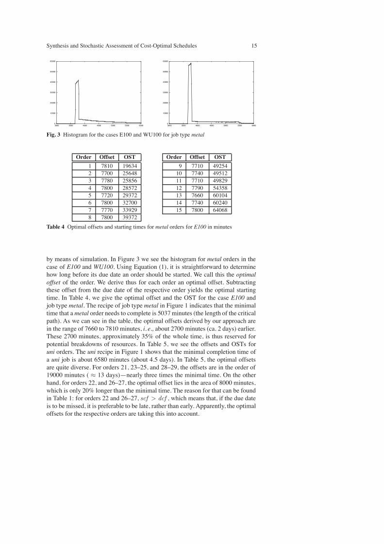
Fig. 3 Histogram for the cases E100 and WU100 for job type metal

Order Offset OST1 7810 196342 7700 256483 7780 258564 7800 285725 7720 293726 7800 327007 7770 339298 7800 39372

Order Offset OST9 7710 4925410 7740 4951211 7710 4982912 7790 5435813 7660 6010414 7740 6024015 7800 64068

Table 4 Optimal offsets and starting times for metal orders for E100 in minutes

by means of simulation. In Figure 3 we see the histogram for metal orders in thecase of E100 and WU100. Using Equation (1), it is straightforward to determinehow long before its due date an order should be started. We call this the optimaloffset of the order. We derive thus for each order an optimal offset. Subtractingthese offset from the due date of the respective order yields the optimal startingtime. In Table 4, we give the optimal offset and the OST for the case E100 andjob type metal. The recipe of job type metal in Figure 1 indicates that the minimaltime that ametal order needs to complete is 5037minutes (the length of the criticalpath). As we can see in the table, the optimal offsets derived by our approach arein the range of 7660 to 7810 minutes, i. e., about 2700 minutes (ca. 2 days) earlier.These 2700 minutes, approximately 35% of the whole time, is thus reserved forpotential breakdowns of resources. In Table 5, we see the offsets and OSTs foruni orders. The uni recipe in Figure 1 shows that the minimal completion time ofa uni job is about 6580 minutes (about 4.5 days). In Table 5, the optimal offsetsare quite diverse. For orders 21, 23–25, and 28–29, the offsets are in the order of19000 minutes ( $ 13 days)—nearly three times the minimal time. On the otherhand, for orders 22, and 26–27, the optimal offset lies in the area of 8000 minutes,which is only 20% longer than the minimal time. The reason for that can be foundin Table 1: for orders 22 and 26–27, scf > dcf , which means that, if the due dateis to be missed, it is preferable to be late, rather than early. Apparently, the optimaloffsets for the respective orders are taking this into account.

16 A. Mader et al.

Order Offset OST21 19390 3045922 8320 4162823 18920 4376424 18710 4400425 19070 50580

Order Offset OST26 8110 6058827 7930 6178828 18810 7712429 19070 85764

Table 5 Optimal offsets and starting times for uni orders for E100 in minutes

5.3 Generation of schedules

Using UPPAAL CORA, we produced 6 sets of schedules:

– 10 Schedules, using netto processing times. We call this class S.NPT.– 10 Schedules, using extended processing times. We call this class S.EPT.– Four classes of schedules with 10 schedules each, taking the optimal startingtimes of the four scenarios E100, E31, WU100, and WU31 into account (cf.Section 5.1). We call these four classes of schedules S.E100, S.E31, S.WU100,and S.WU31, respectively.

The objective function for the S.NPT and S.EPT schedules was to meet thedue dates as good as possible, causing costs for storage and delay as in the casedescription.

For the four classes S.E100, S.E31, S.WU100, and S.WU31, the objective func-tion for the schedule synthesis was to find schedules that have the starting timesof orders as close as possible to the OSTs and that have resolved the resourceconflicts.

As explained in Section 3.1, the search strategy we use is best cost randomdepth first. Experiments show that this search strategy gives the best results: thestate space is too big to be traversed completely. Due to the randomness and thesize of the search space we got schedules of different quality, i. e., with high costvariations. In order to generate a set of ten schedules we always performed a muchhigher number of schedules, depending on the model the number of experimentsis a factor of 3–10 higher. A single experiment, however, takes less than a minutein most cases, less than 3 minutes in all cases.

The most efficient heuristic used is the limitation of the number of orders thatare processed at each moment. The upper boundwe chose is 5, and was found aftera number of experiments. It is plausible, considering the bottleneck resources:the dose spinners, that are available twice, but have to be used by every order,the disperging line, and to some extent also the mixing vessels. Moreover, wechose a greedy strategy for resource distribution. If several orders are waiting fora resource, the the one who gets the resource is chosen nondeterministically, i.e.we do not have a waiting queue model. Heuristics reducing the time windows forstarting orders, were also applied. Much effort went to this fine-tuning, which isjustified by the goal to find schedules as close as possible to the OSTs.


5.4 Analysis by simulation

As explained in Section 4, our method to assess the quality of deterministic sched-ules is stochastic simulation. In this section we will present the results of the sim-ulations.

In this experiment, we simulated seven classes of schedules. The first six classesare those generated with UPPAAL CORA, as described in the previous section. Theseventh class is a set of four schedules, based on the OST only. Since we take in ourapproach only the starting times of orders into account, it is possible to regard theoptimal starting times already as schedule as well: we start each order exactly at itsoptimal starting time. Thus, for each of the four schedule classes S.E100, S.E31,SWU100, and S.WU31 we have one extra schedule, defined by the OSTs for thatclass. We call the respective schedule S.OST.E100, S.OST.E31, S.OST.WU100, andS.OST.WU31.

Our measure of interest is, for each schedule, the mean total cost that accu-mulates during the execution of all 29 orders. We simulated all schedules of allconsidered classes. The mean value is estimated with a relative confidence interval< 10% and a confidence level of 99%.

The schedules in class S.NPT and S.EPT were simulated for all the scenar-ios E100, E31, WU100, and WU31. The schedules S.E100, S.E31, SWU100, andS.WU31 were each only simulated with the corresponding scenario, i. e., S.E100with E100, etc.

In order to reduce the size of the tables with the results, we do not presentthe outcome for all schedules per class, but rather the average (E[·]) and relativestandard deviation (coefficient of variation cv) of the respective outcomes. Thenumeric results are summarised in Table 6.

5.5 Interpretation of Simulation Results

5.5.1 Comparison of the S.NPT and S.EPTschedules. The average costs of theS.NPT schedules range from 8 Mio. to 12 Mio., depending on the chosen scenario.The relative standard deviation ranges from ca. 12 to 17%. This shows that, eventhough all schedules in this class resolve resource conflicts, the way it is done hasan influence on the costs that are incurred.

The average costs of the S.NPT schedules are the highest in the whole table.This is not surprising, since these schedules do not take the failure of resource intoaccount at all. Therefore, for each order the probability to overshoot the due dateby a considerable amount of time is very high. The S.NPT numbers show how badcosts can become.

The average cost of schedules in the S.EPT class range from ca. 2.5 Mio. to 6Mio., depending on the chosen failure scenario. The relative standard deviation isbetween 17% and 38%. The S.EPT schedules are better than the S.NPT schedules.We explain this by the fact that more time is calculated for the execution of eachtask, and thus for each order. The numbers suggest that S.EPT can indeed helpsaving considerable costs, compared to the S.NPT schedules.

18 A. Mader et al.Failuremodelusedforschedulegeneration

Failure model used for schedule analysisSchedule set Measure E100 E31 WU100 WU31

S.NPT E[·] 12.131.001 9.628.586 9.720.134 8.568.726cv 11.88% 15.51% 14.16% 16.97%

S.EPT E[·] 5.907.007 3.340.511 3.800.883 2.530.444cv 17.17% 29.28% 26% 37.12%

S.E100 E[·] 1.683.969cv 1.93%

S.E31 E[·] 855.446cv 3.76%

S.WU100 E[·] 1.313.474cv 4.79%

S.WU31 E[·] 785.304cv 7.47%

S.OST.E100 1.732.719S.OST.E31 1.445.109

S.OST.WU100 2.209.187S.OST.WU31 2.165.868

Table 6 Results for total cost for different schedules

The variation in the costs for the S.NPT and S.EPT schedules confirm that thereare good schedules and bad schedules. At this point we are not able to determinea priori, what schedule is a good one without simulation.

5.5.2 Comparison of the S.EPT and the S.E/S.WU schedules. We consider firstthe S.E100 case. Table 6 shows, that the average costs incurred by these sched-ules is about 1.7 Mio. The relative standard deviation is with 1.93% very low. Wecan see, that the average cost of the S.E100 schedules is only 28.5% of the averagecost of the S.EPT schedules for the E100 scenario. Since the variation of the S.EPTschedules is in the order of 17%, we can assume a best-case schedule which is in-deed 17% better than the average. On the other hand, we can assume that there is aS.E100 schedule that is 1.93%worse than the average. Setting best-case and worst-case schedules in relation, the costs of the worst-case S.E100 schedule would stillbe only 35% of the best-case S.EPT schedule.

For the S.E31 schedules, the average costs are about 0.86 Mio., with a relativestandard deviation of 3.8%. This is 25.6% of the costs of the S.EPT schedulesin the E31 scenario. Assuming again best-case/worst-case schedules, the S.E31schedule would still cost only 38% of the S.EPT schedule.

The S.WU100 schedules reduce the costs to 34.5% of the S.EPT schedules,and, assuming the best-case/worst-case again, the cost is still reduced to about49%.

Finally, the S.WU31 cost on average only 31% of the S.EPT schedules, and inthe extreme case, still only 53%.


These results lead us to the main conclusion of this paper: OST schedules arein general cheaper than EPT schedules, and thus better.

5.5.3 Comparison of S.E/S.WU and S.OST.E/S.OST.WU schedules. The sched-ules in the S.E/S.WU classes have been generated with UPPAAL CORA. Since theoptimal starting times can also be seen as schedules themselves, the question ariseswhether UPPAAL CORA is needed at all, and if these S.OST.E/S.OST.WU schedulesare not actually sufficient.

The numbers in Table 6 show that this is in general not the case. Even thoughfor the S.E100/S.OST.E100, the costs are very close (around 1.7Mio.), for the othercases the differences become more pronounced: the UPPAAL schedules generate60%, in the WU31 case even only 36% of the costs of the corresponding OSTschedules.

Our explanation for that is that the schedules generated with UPPAAL CORAdo resolve resource conflicts by letting orders start earlier (if scf <dcf ), or later(if scf >dcf ). Thus, the effect is that the probability to complete the order on theexpensive side of the cost function is reduced. Consequently, the step of producingrefined OST with UPPAAL CORA is indeed necessary to reduce the mean total costsfurther.

5.6 Robustness of the OST approach

The results of the previous section indicate that our approach to use OST sched-ules to reduce the mean total costs of a batch of orders is indeed a promising one.In this section we show that even if we make inaccurate assumptions on the fail-ure distributions, and thus work with inaccurate OSTs to generate schedules, inall cases the costs are not higher than for the EPT approach, and in most casessignificantly better. In order to find out how stable our approach is, we have sim-

E100 E31 WU100 WU31S.EPT 5.907.007 3.340.511 3.800.883 2.530.444S.E100 1.683.969 1.105.239 1.139.555 1.079.691S.E31 2.232.010 855.446 986.859 702.696

S.WU100 3.047.240 1.070.889 1.313.474 684.322S.WU31 3.842.751 1.416.179 1.769.831 785.304

Table 7 Average mean total costs for all OST schedule with all scenarios

ulated all S.E/S.WU schedules also with the parameters for which the scheduleswhere not generated for. We would expect that the simulations with the “proper”parameters should always give lower costs than the others. This is however notalways the case. In Table 7, we see the averages for all combinations of scheduleclasses and failure scenarios. For comparison, we have also repeated the valuesfor the S.EPT schedules from Table 6. Also the values set in boldface come from

20 A. Mader et al.

the same Table. For the case of scenario E100 we see that the schedules in classS.E100 produce minimal cost: the non-diagonal values in the respective columnare all much higher. The same holds still for the case E31: the schedules of classS.E31 are the lowest in the column.

The situation is different for the WU scenarios. In both cases, the correspond-ing S.WU schedules do not yield the lowest cost. In case of WU100 it would bebetter to use a schedule from the S.E31 class. In case of WU31, it would be betterto use one from S.WU100.

The cause of this phenomenon is subject to further research. Nevertheless,even though wrong assumptions on distributions might give not the best results,a comparison with the S.EPT results shows that our OST approach produces stillsubstantially better results.

6 Conclusions

In this article, we present an alternative to the EPT approach to generate schedulesthat take the possible failures of resources into account. The pivotal elements of ourapproach are the so-called optimal start times of orders. These OSTs are estimatedby means of simulation and straightforwardmathematical derivations. They reflectrelease times of orders for which the expected cost incurred by the orders areminimal. We use the OSTs as input to our schedule synthesizer, the model-checkerUPPAAL CORA.

We assess the properties of all generated schedules by means of stochasticsimulation. The simulation models, described in the modeling language MODEST,are simulated with MOBIUS. The simulation models comprise resources prone tofailure, the recipes, and the schedule in question.We have considered four differentcases of failure behaviour for the estimation of OSTs, generation of schedules andthe simulation of schedules.

The simulation results show that the schedules that we have derived with theOST approach are in all four considered scenarios substantially cheaper than theschedules derived with the EPT approach. Our approach is robust in the sense that,even if assumptions on the failure behaviour of resources are inaccurate, the OSTschedules still incur lower costs then their EPT counterparts.

Our main conclusion is using optimal starting times for the generation ofschedules to be a favourable alternative to the EPT approach.

However, it is also clear that our approach could be improved by more fine tun-ing. Relevant questions are what the right assumptions for derivation of the OSTsare, e. g., what the best estimates for distribution of resource failure are, and whatthe best assumptions on the background load of a system. Then, taking OSTs as abasis for derivation of schedules, the question is what is a schedule that approxi-mates the OSTs best. We suggested a cost function with an obvious intuition, butpossibly there are better strategies. Another direction could be to be more explicitover the load in a system. There are moments with low load, and others wherethe load is high. Our OSTs are all based on high load, for moments with low loadthey are too pessimistic. We could calculate different OSTs for different loads and


apply the best fitting OST during scheduling when it is clear howmany concurrentorders have to be processed in the close future.

Also, the scheduling strategy we followed in both schedule synthesis and simu-lation is greedy, and when there are several tasks waiting for a resource, one task ischosen nondeterministically that gets the resource. Possibly other strategies, suchas activeness (non-laziness), non-overtaking, or waiting-queues could give betterresults.

The tools we used, UPPAAL CORA and MOBIUS have the necessary modellingand processing capabilities that are needed for the demonstration of our approach.However, these tools do not yet have industrial strength. Modelling effort that, inprinciple, can be automated was done by hand here, which is a time-consumingprocess. For an industrial application, modelling should be mechanized and per-formed with tool-support. Nevertheless, UPPAAL CORA and M OBIUS are undercontinuous improvement, aiming at industrial applicability.

Acknowledgements We give our thanks to Ed Brinksma for discussion on the approach,and to Martijn Hendriks and Gerd Behrmann, who helped us with models and tools.

References

1. Rajeev Alur and David L. Dill. A theory of timed automata. Theoretical ComputerScience, 126(2):183–235, 1994.

2. Rajeev Alur, Salvatore La Torre, and George J. Pappas. Optimal paths in weightedtimed automata. In Maria Domenica Di Benedetto and Alberto Sangiovanni-Vincentelli, editors, Hybrid Systems: Computation and Control; . . . HSCC, volume2034 of LNCS, Berlin, 2001. Springer.

3. AMETIST, IST project ist-2001-35304. http://ametist.cs.utwente.nl/.4. Tobias Amnell, Gerd Behrmann, Johan Bengtsson, Pedro R. D’Argenio, AlexandreDavid, Ansgar Fehnker, Thomas Hune, Bertrand Jeannet, Kim G. Larsen, M. OliverMoller, Paul Pettersson, Carsten Weise, and Wang Yi. UPPAAL: Now, next, and fu-ture. In Franck Cassez, Claude Jard, Brigitte Rozoy, and Mark Dermot Ryan, editors,Modeling and Verification of Parallel Processes: 4th summer school, MOVEP 2000,volume 2067 of LNCS, pages 99–124, Berlin, 2001. Springer.

5. Gerd Behrmann, Ed Brinksma, Martijn Hendriks, and Angelika Mader. Productionscheduling by reachability analysis: A case study. In 19th IEEE International Paralleland Distributed Processing Symposium: Workshop on Parallel and Distributed Real-Time Systems; WPDRTS, page paper 140a, Los Alamitos, California, April 2005. IEEEComputer Society.

6. Gerd Behrmann, Ed Brinksma, Martijn Hendriks, and Angelika Mader. Schedulinglacquer production by reachability analysis: a case study. In P. Horacek, M. Simandl,and P. Zitek, editors, Preprints of the 16th IFACWorld Congress: Prague [DVD], pagesMo–A17–TO/3, Laxenburg, Austria, July 2005. International Federation of AutomaticControl.

7. Gerd Behrmann, Alexandre David, and Kim G. Larsen. A tutorial on UPPAAL. InMarco Bernardo and Flavio Corradini, editors, Formal Methods for the Design ofReal-Time Systems: . . . SFM-RT 2004, number 3185 in LNCS, pages 200–236, Berlin,September 2004. Springer.

22 A. Mader et al.

8. Gerd Behrmann, Ansgar Fehnker, Thomas Hune, Kim Larsen, Paul Petterson, JudiRomijn, and Frits Vaandrager. Minimum-cost reachability for priced timed automata.In Maria Domenica Di Benedetto and Alberto Sangiovanni-Vincentelli, editors,HybridSystems: Computation and Control; . . . HSCC, volume 2034 of LNCS, pages 147–161,Berlin, 2001. Springer.

9. Gerd Behrmann, Ansgar Fehnker, Thomas Hune, Kim G. Larsen, Paul Petterson, andJudi Romijn. Guiding and cost-optimality in UPPAAL. In Lina Khatib and CharlesPecheur, editors, Model-Based Validation of Intelligence: Papers from 2001 AAAISpring Symposium. AAAI, 2001.

10. H. C. Bohnenkamp, H. Hermanns, R. Klaren, A. Mader, and Y. S. Usenko. Synthe-sis and stochastic assessment of schedules for lacquer production. In First Interna-tional Conference on the Quantitiative Evaluation of Systems: QEST, pages 28–37,Los Alamitos, CA, September 2004. IEEE Computer Society.

11. Henrik Bohnenkamp, Tod Courtney, David Daly, Salem Derisavi, Holger Hermanns,Joost-Pieter Katoen, Vinh Vi Lam, and William H. Sanders. On integrating theMOBIUS and MODEST modeling tools. In 2003 International Conference on Depend-able Systems and Networks: . . . DSN, page 671, Los Alamitos, CA, 2003. IEEE Com-puter Society.

12. Henrik Bohnenkamp, Pedro R. D’Argenio, Holger Hermanns, and Joost-Pieter Katoen.MoDeST: A compositional modeling formalism for hard and softly timed systems.Technical Report TR-CTIT-04-46, Centre for Telematics and Information Technology,University of Twente, Enschede, The Netherlands, November 2004.

13. Henrik Bohnenkamp, Holger Hermanns, Joost-Pieter Katoen, and Ric Klaren. TheMODEST modeling tool and its implementation. In Peter Kemper and William H.Sanders, editors, Computer Performance Evaluation: . . . TOOLS, volume 2794 ofLNCS, pages 116–133, Berlin, 2003. Springer.

14. Edmund M. Clarke, Jr., Orna Grumberg, and Doron A. Peled. Model Checking. MITPress, Cambridge, MA, 1999.

15. UPPAAL CORA home page. www.cs.aau.dk/!behrmann/cora/.16. David Daly, Daniel D. Deavours, Jay M. Doyle, Patrick G. Webster, and William H.

Sanders. Mobius: An extensible tool for performance and dependability modeling.In Boudewijn R. Haverkort, Henrik C. Bohnenkamp, and Connie U. Smith, editors,Computer Performance Evaluation: . . . TOOLS, volume 1786 of LNCS, pages 332–336, Berlin, 2000. Springer. Tool Description.

17. Pedro R. D’Argenio, Holger Hermanns, Joost-Pieter Katoen, and Ric Klaren.MoDeST: A modelling and description language for stochastic timed systems. In Lucade Alfaro and Stephen Gilmore, editors, Process Algebra and Probabilistic Methods:. . . PAPM–PROBMIV, volume 2165 of LNCS, pages 87–104, Berlin, 2001. Springer.

18. Daniel D. Deavours, Graham Clark, Tod Courtney, David Daly, Salem Derasavi, Jay M.Doyle, William H. Sanders, and Patrick G. Webster. The Mobius framework and itsimplementation. IEEE Transactions on Software Engineering, 28(10):956–969, 2002.

19. Erik L. Demeulemeester and Willy S. Herroelen. Project Scheduling: A ResearchHandbook. Kluwer, Boston, 2002.

20. Peter G. Harrison and Naresh M. Patel. Performance Modelling of CommunicationNetworks and Computer Architectures. Addison-Wesley, Wokingham, 1993.

21. Gerald J. Holzmann. The SPIN model checker: primer and reference manual. Addison-Wesley, Boston, 2004.

22. Michael Huth and Mark Ryan. Logic in Computer Science: Modelling and reasoningabout systems. Cambridge University Press, Cambridge, 2000.

23. Jeff Magee and Jeff Kramer. Concurrency: State Models and Java Programs. Wiley,Chichester, 1999.


24. Sebastian Panek, Sebastian Engell, and Cathrin Lessner. Scheduling of a pipelessmulti-product batch plant using mixed-integer programming combined with heuristics.In Luis Puigjaner and Antonio Espuna, editors, European Symposium on ComputerAided Process Engineering 15: . . . ESCAPE-15, volume 20 A/B of Computer-aidedchemical engineering, pages 1033–1038, Amsterdam, 2005. Elsevier.

25. Michael Pinedo. Scheduling: Theory, Algorithms, and Systems. Prentice Hall, UpperSaddle, NJ, 2nd edition, 2002.

26. UPPAAL home page. http://www.uppaal.com.

Synthesis and stochastic assessment of cost-optimal schedules

Documents

Transcript of Synthesis and stochastic assessment of cost-optimal schedules