Optimal Stochastic Control in the Interception Problem of a ...
15
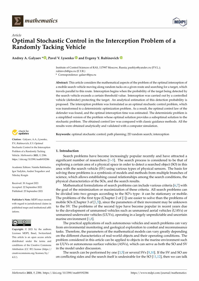
mathematics Article Optimal Stochastic Control in the Interception Problem of a Randomly Tacking Vehicle Andrey A. Galyaev * , Pavel V. Lysenko and Evgeny Y. Rubinovich Citation: Galyaev, A.A.; Lysenko, P.V.; Rubinovich, E.Y. Optimal Stochastic Control in the Interception Problem of a Randomly Tacking Vehicle. Mathematics 2021, 9, 2386. https://doi.org/10.3390/math9192386 Academic Editors: Natalia Bakhtadze, Igor Yadykin, Andrei Torgashov and Nikolay Korgin Received: 30 August 2021 Accepted: 22 September 2021 Published: 25 September 2021 Publisher’s Note: MDPI stays neutral with regard to jurisdictional claims in published maps and institutional affil- iations. Copyright: © 2021 by the authors. Licensee MDPI, Basel, Switzerland. This article is an open access article distributed under the terms and conditions of the Creative Commons Attribution (CC BY) license (https:// creativecommons.org/licenses/by/ 4.0/). Institute of Control Sciences of RAS, 117997 Moscow, Russia; [email protected] (P.V.L.); [email protected] (E.Y.R.) * Correspondence: [email protected] Abstract: This article considers the mathematical aspects of the problem of the optimal interception of a mobile search vehicle moving along random tacks on a given route and searching for a target, which travels parallel to this route. Interception begins when the probability of the target being detected by the search vehicle exceeds a certain threshold value. Interception was carried out by a controlled vehicle (defender) protecting the target. An analytical estimation of this detection probability is proposed. The interception problem was formulated as an optimal stochastic control problem, which was transformed to a deterministic optimization problem. As a result, the optimal control law of the defender was found, and the optimal interception time was estimated. The deterministic problem is a simplified version of the problem whose optimal solution provides a suboptimal solution to the stochastic problem. The obtained control law was compared with classic guidance methods. All the results were obtained analytically and validated with a computer simulation. Keywords: optimal stochastic control; path planning; 2D random search; interception 1. Introduction Search problems have become increasingly popular recently and have attracted a significant number of researchers [1–5]. The search process is considered to be that of exploring a certain area of a physical space in order to detect a searched object (SO) in this area with the search vehicle (SV) using various types of physical sensors. The basis for solving these problems is a symbiosis of models and methods from multiple branches of science, which allows establishing causal relationships among the search conditions, the physical characteristics of the SOs, and the search results. Mathematical formulations of search problems can include various criteria [6,7] with the goal of the minimization or maximization of these criteria. All search problems can be divided into two groups according to the SO’s type: it can be stationary or mobile. The problems of the first type (Chapter 2 of [1]) are easier to solve than the problems of mobile SOs (Chapter 3 of [1,5]), since the parameters of their movement may be unknown to the SV. The problems of the second type have become popular in recent years due to the development of unmanned vehicles such as unmanned aerial vehicles (UAVs) or unmanned underwater vehicles (UUVs), operating in a largely unpredictable and uncertain marine environment [1,8]. The practical applications of such autonomous vehicles and search problems can vary from environmental monitoring and geological exploration to combat and reconnaissance tasks. Therefore, the parameters of the mathematical models can vary greatly depending on the different characteristics of real-world objects and their operating conditions. The problem considered in this article can be applied to objects in the marine environment such as UUVs or autonomous surface vehicles (ASVs), which can serve as both the SO and SV in the model under discussion. The search can be performed by one [3,5] or several SVs [9,10]. If the SV and SO are on conflicting sides and the search itself is undesirable for the SO [11,12], then we can talk Mathematics 2021, 9, 2386. https://doi.org/10.3390/math9192386 https://www.mdpi.com/journal/mathematics
-
Upload
khangminh22 -
Category
Documents
-
view
7 -
download
0
Transcript of Optimal Stochastic Control in the Interception Problem of a ...
mathematics
Article
Optimal Stochastic Control in the Interception Problem of aRandomly Tacking Vehicle
Andrey A. Galyaev * , Pavel V. Lysenko and Evgeny Y. Rubinovich
�����������������
Citation: Galyaev, A.A.; Lysenko,
P.V.; Rubinovich, E.Y. Optimal
Stochastic Control in the Interception
Problem of a Randomly Tacking
Vehicle. Mathematics 2021, 9, 2386.
https://doi.org/10.3390/math9192386
Academic Editors: Natalia Bakhtadze,
Igor Yadykin, Andrei Torgashov and
Nikolay Korgin
Received: 30 August 2021
Accepted: 22 September 2021
Published: 25 September 2021
Publisher’s Note: MDPI stays neutral
with regard to jurisdictional claims in
published maps and institutional affil-
iations.
Copyright: © 2021 by the authors.
Licensee MDPI, Basel, Switzerland.
This article is an open access article
distributed under the terms and
conditions of the Creative Commons
Attribution (CC BY) license (https://
creativecommons.org/licenses/by/
4.0/).
Institute of Control Sciences of RAS, 117997 Moscow, Russia; [email protected] (P.V.L.);[email protected] (E.Y.R.)* Correspondence: [email protected]
Abstract: This article considers the mathematical aspects of the problem of the optimal interception ofa mobile search vehicle moving along random tacks on a given route and searching for a target, whichtravels parallel to this route. Interception begins when the probability of the target being detected bythe search vehicle exceeds a certain threshold value. Interception was carried out by a controlledvehicle (defender) protecting the target. An analytical estimation of this detection probability isproposed. The interception problem was formulated as an optimal stochastic control problem, whichwas transformed to a deterministic optimization problem. As a result, the optimal control law of thedefender was found, and the optimal interception time was estimated. The deterministic problem isa simplified version of the problem whose optimal solution provides a suboptimal solution to thestochastic problem. The obtained control law was compared with classic guidance methods. All theresults were obtained analytically and validated with a computer simulation.
Keywords: optimal stochastic control; path planning; 2D random search; interception
1. Introduction
Search problems have become increasingly popular recently and have attracted asignificant number of researchers [1–5]. The search process is considered to be that ofexploring a certain area of a physical space in order to detect a searched object (SO) in thisarea with the search vehicle (SV) using various types of physical sensors. The basis forsolving these problems is a symbiosis of models and methods from multiple branches ofscience, which allows establishing causal relationships among the search conditions, thephysical characteristics of the SOs, and the search results.
Mathematical formulations of search problems can include various criteria [6,7] withthe goal of the minimization or maximization of these criteria. All search problems canbe divided into two groups according to the SO’s type: it can be stationary or mobile.The problems of the first type (Chapter 2 of [1]) are easier to solve than the problems ofmobile SOs (Chapter 3 of [1,5]), since the parameters of their movement may be unknownto the SV. The problems of the second type have become popular in recent years dueto the development of unmanned vehicles such as unmanned aerial vehicles (UAVs) orunmanned underwater vehicles (UUVs), operating in a largely unpredictable and uncertainmarine environment [1,8].
The practical applications of such autonomous vehicles and search problems can varyfrom environmental monitoring and geological exploration to combat and reconnaissancetasks. Therefore, the parameters of the mathematical models can vary greatly dependingon the different characteristics of real-world objects and their operating conditions. Theproblem considered in this article can be applied to objects in the marine environment suchas UUVs or autonomous surface vehicles (ASVs), which can serve as both the SO and SVin the model under discussion.
The search can be performed by one [3,5] or several SVs [9,10]. If the SV and SO areon conflicting sides and the search itself is undesirable for the SO [11,12], then we can talk
Mathematics 2021, 9, 2386. https://doi.org/10.3390/math9192386 https://www.mdpi.com/journal/mathematics

Mathematics 2021, 9, 2386 2 of 15
about the so-called threat environment [13,14]. Several SVs can be connected in a networkstructure and form a dynamically changing threat map [10,15]. The task of the SO (UUV orUAV) in this case is to avoid these threats while moving. The trajectory planning problemcan be formulated for the SO when the threat mapping is known. If the dynamics of the SOis also known, then these problems are classical problems of deterministic optimal control.
If the SV presents a danger to the SO, the problem of interception can be consid-ered. There is a vast class of such problems with various formulations and models of themoving vehicles. These models may include restrictions on the maneuverability of thevehicles [16–18]. Moreover, the problem can be considered optimal if any criterion, asfor example, the intercept time, must be minimized [19–21]. In most problems studied inthe literature, the intercepted vehicle moves along a given programmed trajectory [22].Meanwhile, real vehicles as a rule move in a stochastic way, and this case is considered inthe presented article.
The article relates to various branches of mathematics, such as stochastic control,guidance, information processing and search, and optimization, and is devoted to theproblem of the optimal interception of an SV that moves randomly on tacks along agiven course and searches for a target SO. The interception is carried out by a controlledmobile vehicle protecting the target SO. The presence of an arbitrarily maneuvering searchvehicle requires an adequate mathematical formalization in the form of a stochastic controlproblem. The maneuvering process can be conveniently formalized using a jump-likeMarkov process with a given state vector and a given matrix of the transition intensitiesbetween these states. Such a model allows us to describe the trajectory of the SV in the formof a linear stochastic differential equation, which makes it possible to obtain the equationsof the evolution of the mathematical expectation and variance. These equations allow us toformulate the problem of SV interception by the controlled vehicle with the criterion ofa predicted miss or with a given mathematical expectation of a miss at the final positionof the SV [16–21]. The purpose of the article is to find an interception trajectory of thecontrolled defender vehicle as a result of solving the optimal stochastic control problem andcomparing this trajectory with classical guidance algorithms such as the pursuit guidancemethod and the method of proportional navigation guidance [23–25].
The considered problem belongs to the “attacker–target–defender” type [26–28], theessence of which is a counteraction to the SV (attacker) from the SO (target), which can bea certain strategically important mobile vehicle, by using an autonomous attacking roboticcomplex (defender), for example an UAV or UUV.
In this article, by SV, we mean a vehicle moving programmatically or randomly ona plane equipped with a circular detection zone of a fixed radius. The goal of the SV isto detect the SO, i.e., to cover the point of the plane depicting the SO with its detectionzone and maximize some functional that characterizes the reliability of detecting the SOin this zone. The reliability of the detection (probability of correct classification) of the SVmay depend on various physical factors, in particular on the time spent by the SO in thedetection zone, its current distance from the SV, the direction of the velocity vector of theSO, etc. [29].
We considered the SO to be able to observe the real trajectory of the SV and evalu-ate the characteristics of its movement, i.e., current coordinates and components of thevelocity vector. At some point in time, the SO releases a mobile defender, which movesautonomously and stealthily and does not have a communication channel with the SO.It was also assumed that the defender can evaluate the current motion characteristics ofthe SV using its passive onboard sensors. The stealthiness of the defender is provided, inparticular, with its low velocity.
The proposed work has the following structure. In Section 2, the model of the SVwith a given detection zone is considered. Section 3 contains a statistic description of thedetection probability of the SO moving along a straight-line trajectory. In Section 4, theinterception problem is formulated as an optimal stochastic control problem. This problemis analytically solved in Section 5, and the obtained results are discussed and illustrated
Mathematics 2021, 9, 2386 3 of 15
with simulation examples in Section 6. Section 7 concludes the article and suggests thedirection for future work.
2. Model of the SV’s Movement on Tacks
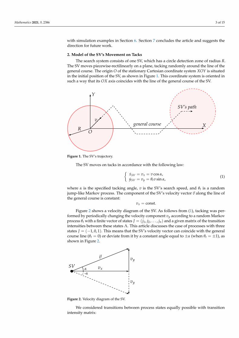
The search system consists of one SV, which has a circle detection zone of radius R.The SV moves piecewise-rectilinearly on a plane, tacking randomly around the line of thegeneral course. The origin O of the stationary Cartesian coordinate system XOY is situatedin the initial position of the SV, as shown in Figure 1. This coordinate system is oriented insuch a way that its OX axis coincides with the line of the general course of the SV.
OXgeneral course
Y
R
SV’s path
v
Figure 1. The SV’s trajectory.
The SV moves on tacks in accordance with the following law:{xSV = vx = v cos α,ySV = vy = θtv sin α,
(1)
where α is the specified tacking angle, v is the SV’s search speed, and θt is a randomjump-like Markov process. The component of the SV’s velocity vector ~v along the line ofthe general course is constant:
vx = const.
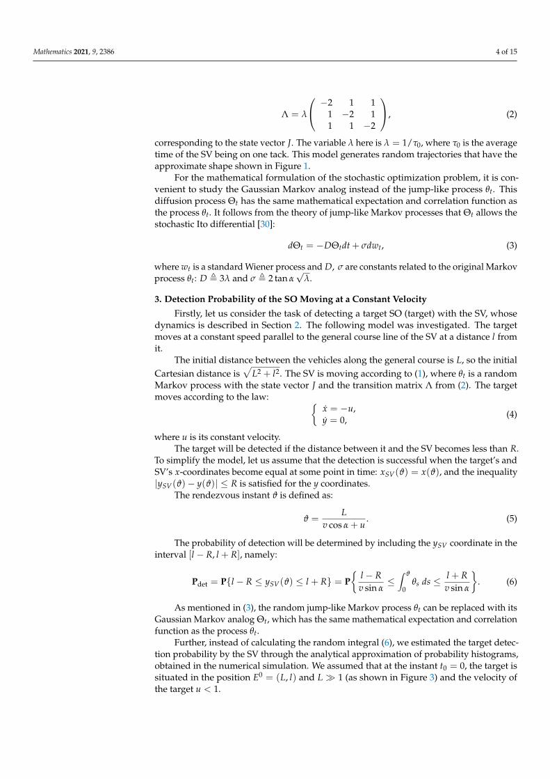
Figure 2 shows a velocity diagram of the SV. As follows from (1), tacking was per-formed by periodically changing the velocity component vy according to a random Markovprocess θt with a finite vector of states J = (j1, j2, . . . , jn) and a given matrix of the transitionintensities between these states Λ. This article discusses the case of processes with threestates J = (−1, 0, 1). This means that the SV’s velocity vector can coincide with the generalcourse line (θt = 0) or deviate from it by a constant angle equal to ±α (when θt = ±1), asshown in Figure 2.
SV vx
~v vy
α
vy
-α
Figure 2. Velocity diagram of the SV.
We considered transitions between process states equally possible with transitionintensity matrix:
Mathematics 2021, 9, 2386 4 of 15
Λ = λ
−2 1 11 −2 11 1 −2
, (2)
corresponding to the state vector J. The variable λ here is λ = 1/τ0, where τ0 is the averagetime of the SV being on one tack. This model generates random trajectories that have theapproximate shape shown in Figure 1.
For the mathematical formulation of the stochastic optimization problem, it is con-venient to study the Gaussian Markov analog instead of the jump-like process θt. Thisdiffusion process Θt has the same mathematical expectation and correlation function asthe process θt. It follows from the theory of jump-like Markov processes that Θt allows thestochastic Ito differential [30]:
dΘt = −DΘtdt + σdwt, (3)
where wt is a standard Wiener process and D, σ are constants related to the original Markovprocess θt: D , 3λ and σ , 2 tan α
√λ.
3. Detection Probability of the SO Moving at a Constant Velocity
Firstly, let us consider the task of detecting a target SO (target) with the SV, whosedynamics is described in Section 2. The following model was investigated. The targetmoves at a constant speed parallel to the general course line of the SV at a distance l fromit.
The initial distance between the vehicles along the general course is L, so the initialCartesian distance is
√L2 + l2. The SV is moving according to (1), where θt is a random
Markov process with the state vector J and the transition matrix Λ from (2). The targetmoves according to the law: {
x = −u,y = 0,
(4)
where u is its constant velocity.The target will be detected if the distance between it and the SV becomes less than R.
To simplify the model, let us assume that the detection is successful when the target’s andSV’s x-coordinates become equal at some point in time: xSV(ϑ) = x(ϑ), and the inequality|ySV(ϑ)− y(ϑ)| ≤ R is satisfied for the y coordinates.
The rendezvous instant ϑ is defined as:
ϑ =L
v cos α + u. (5)
The probability of detection will be determined by including the ySV coordinate in theinterval [l − R, l + R], namely:
Pdet = P{l − R ≤ ySV(ϑ) ≤ l + R} = P{
l − Rv sin α
≤∫ ϑ
0θs ds ≤ l + R
v sin α
}. (6)
As mentioned in (3), the random jump-like Markov process θt can be replaced with itsGaussian Markov analog Θt, which has the same mathematical expectation and correlationfunction as the process θt.
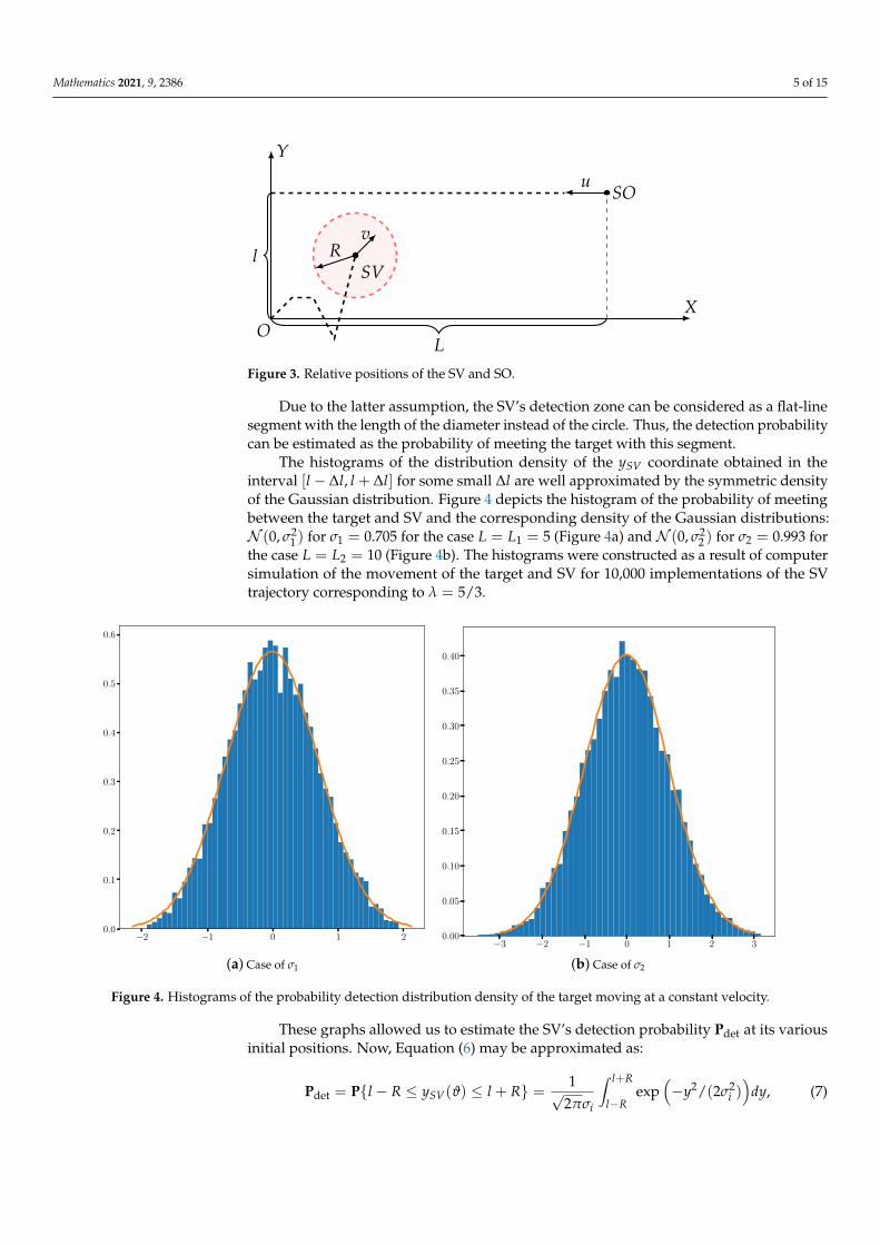
Further, instead of calculating the random integral (6), we estimated the target detec-tion probability by the SV through the analytical approximation of probability histograms,obtained in the numerical simulation. We assumed that at the instant t0 = 0, the target issituated in the position E0 = (L, l) and L � 1 (as shown in Figure 3) and the velocity ofthe target u < 1.
Mathematics 2021, 9, 2386 5 of 15
SV
vR
OX
Y
SOu
l
LFigure 3. Relative positions of the SV and SO.
Due to the latter assumption, the SV’s detection zone can be considered as a flat-linesegment with the length of the diameter instead of the circle. Thus, the detection probabilitycan be estimated as the probability of meeting the target with this segment.
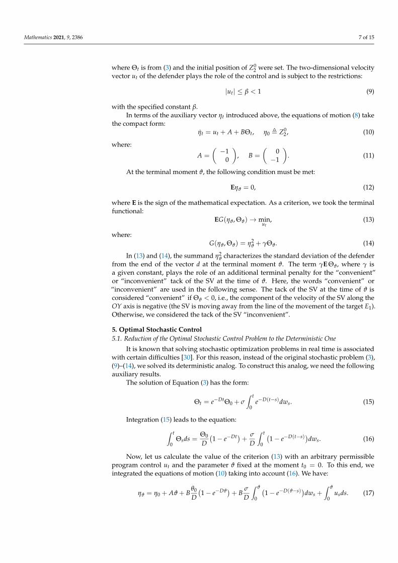
The histograms of the distribution density of the ySV coordinate obtained in theinterval [l − ∆l, l + ∆l] for some small ∆l are well approximated by the symmetric densityof the Gaussian distribution. Figure 4 depicts the histogram of the probability of meetingbetween the target and SV and the corresponding density of the Gaussian distributions:N (0, σ2
1 ) for σ1 = 0.705 for the case L = L1 = 5 (Figure 4a) and N (0, σ22 ) for σ2 = 0.993 for
the case L = L2 = 10 (Figure 4b). The histograms were constructed as a result of computersimulation of the movement of the target and SV for 10,000 implementations of the SVtrajectory corresponding to λ = 5/3.
−2 −1 0 1 20.0
0.1
0.2
0.3
0.4
0.5
0.6
(a) Case of σ1
−3 −2 −1 0 1 2 30.00
0.05
0.10
0.15
0.20
0.25
0.30
0.35
0.40
(b) Case of σ2
Figure 4. Histograms of the probability detection distribution density of the target moving at a constant velocity.
These graphs allowed us to estimate the SV’s detection probability Pdet at its variousinitial positions. Now, Equation (6) may be approximated as:
Pdet = P{l − R ≤ ySV(ϑ) ≤ l + R} = 1√2πσi
∫ l+R
l−Rexp
(−y2/(2σ2
i ))
dy, (7)

Mathematics 2021, 9, 2386 6 of 15
where σi corresponds to various parameters (Li, li, ui). In particular, when l = l1 = 1.5 andl = l2 = 2.5 for L1 and L2, respectively, these probabilities are presented in Table 1. In allcases, the velocity of the target is u = 0.3. All values are given in a normalized scale.
Table 1. The detection probability of the target Pdet at its various initial positions E0 = (L, l).
L l Pdet
5 1.5 0.2385 2.5 0.017
10 1.5 0.30410 2.5 0.065
Next, we introduced a certain threshold value (security threshold) h < 1 of thepermissible detection probability of Pdet, for example h = 0.07. The situation with Pdet ≤ his considered safe. In this case, the target continues to move in a straight line withoutchanging its course and speed. If Pdet > h, then the situation is considered dangerous. Itwas assumed that in the case of a dangerous situation, the target (to prevent the negativeconsequences of possible detection) uses the mobile defender mentioned in the Introduction,whose task is to intercept the SV with a minimum standard error at a given point in theplane relative to the SV.
The minimization of this miss is associated with the solution of the following optimalstochastic control problem.
4. Optimal Stochastic Control Problem
The problem was considered in a moving Cartesian coordinate system XtOtYt, wherethe origin Ot is associated with the current position Pt of the SV and the axis OtXt isdirected parallel to the SV’s general course. The current position of the defender Et
2 is givenby a two-dimensional vector Zt
2 directed from Ot , Pt to Et2.
Terminal position Eϑ2 of the defender is defined by a given two-dimensional vector d,
as shown in Figure 5. An auxiliary vector ηt , Zt2− d was introduced for a more convenient
formulation of the defender’s optimal control problem.
Ot
XtPt
Yt
R
d
Eϑ2
ηt
Zt2
Et2
Figure 5. Geometry of the problem.
In the selected coordinate system, the equations of the relative motion of the defender–SV system have the form:
Zt2 = ut −
(1
Θt
), ut =
(ut
xut
y
), (8)
Mathematics 2021, 9, 2386 7 of 15
where Θt is from (3) and the initial position of Z02 were set. The two-dimensional velocity
vector ut of the defender plays the role of the control and is subject to the restrictions:
|ut| ≤ β < 1 (9)
with the specified constant β.In terms of the auxiliary vector ηt introduced above, the equations of motion (8) take
the compact form:ηt = ut + A + BΘt, η0 , Z0
2 , (10)
where:
A =
( −10
), B =
(0−1
). (11)
At the terminal moment ϑ, the following condition must be met:
Eηϑ = 0, (12)
where E is the sign of the mathematical expectation. As a criterion, we took the terminalfunctional:
EG(ηϑ, Θϑ)→ minut
, (13)
where:G(ηϑ, Θϑ) = η2
ϑ + γΘϑ. (14)
In (13) and (14), the summand η2ϑ characterizes the standard deviation of the defender
from the end of the vector d at the terminal moment ϑ. The term γE Θϑ, where γ isa given constant, plays the role of an additional terminal penalty for the “convenient”or “inconvenient” tack of the SV at the time of ϑ. Here, the words “convenient” or“inconvenient” are used in the following sense. The tack of the SV at the time of ϑ isconsidered “convenient” if Θϑ < 0, i.e., the component of the velocity of the SV along theOY axis is negative (the SV is moving away from the line of the movement of the target E1).Otherwise, we considered the tack of the SV “inconvenient”.
5. Optimal Stochastic Control5.1. Reduction of the Optimal Stochastic Control Problem to the Deterministic One
It is known that solving stochastic optimization problems in real time is associatedwith certain difficulties [30]. For this reason, instead of the original stochastic problem (3),(9)–(14), we solved its deterministic analog. To construct this analog, we need the followingauxiliary results.
The solution of Equation (3) has the form:
Θt = e−DtΘ0 + σ∫ t
0e−D(t−s)dws. (15)
Integration (15) leads to the equation:∫ t
0Θsds =
Θ0
D(1− e−Dt)+ σ
D
∫ t
0
(1− e−D(t−s))dws. (16)
Now, let us calculate the value of the criterion (13) with an arbitrary permissibleprogram control ut and the parameter ϑ fixed at the moment t0 = 0. To this end, weintegrated the equations of motion (10) taking into account (16). We have:
ηϑ = η0 + Aϑ + Bθ0
D(1− e−Dϑ
)+ B
σ
D
∫ ϑ
0
(1− e−D(ϑ−s))dws +
∫ ϑ
0usds. (17)
Mathematics 2021, 9, 2386 8 of 15
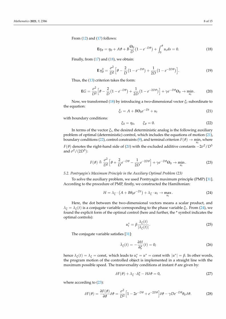
From (12) and (17) follows:
Eηϑ = η0 + Aϑ + BΘ0
D(1− e−Dϑ
)+∫ ϑ
0usds = 0. (18)
Finally, from (17) and (18), we obtain:
E η2ϑ =
σ2
D2
[ϑ− 2
D(1− e−Dϑ
)+
12D(1− e−2Dϑ
)]. (19)
Thus, the (13) criterion takes the form:
EG =σ2
D2
[ϑ− 2
D(1− e−Dϑ
)+
12D(1− e−2Dϑ
)]+ γe−DϑΘ0 → min
ut. (20)
Now, we transformed (18) by introducing a two-dimensional vector ξt subordinate tothe equation:
ξt = A + BΘ0e−Dt + ut (21)
with boundary conditions:ξ0 = η0, ξϑ = 0. (22)
In terms of the vector ξt, the desired deterministic analog is the following auxiliaryproblem of optimal (deterministic) control, which includes the equations of motion (21),boundary conditions (22), control constraints (9), and terminal criterion F(ϑ)→ min
ut, where
F(ϑ) denotes the right-hand side of (20) with the excluded additive constants −2σ2/D3
and σ2/(2D3):
F(ϑ) ,σ2
D2
[ϑ +
2D
e−Dϑ − 12D
e−2Dϑ]+ γe−DϑΘ0 → min
ut. (23)
5.2. Pontryagin’s Maximum Principle in the Auxiliary Optimal Problem (23)
To solve the auxiliary problem, we used Pontryagin maximum principle (PMP) [31].According to the procedure of PMP, firstly, we constructed the Hamiltonian:
H = λξ ·(
A + Bθ0e−Dt)+ λξ · ut → maxut
. (24)
Here, the dot between the two-dimensional vectors means a scalar product, andλξ = λξ(t) is a conjugate variable corresponding to the phase variable ξt. From (24), wefound the explicit form of the optimal control (here and further, the * symbol indicates theoptimal controls):
u∗t = βλξ(t)|λξ(t)|
. (25)
The conjugate variable satisfies [31]:
λξ(t) = −∂H∂ξ
(t) = 0; (26)
hence λξ(t) = λξ = const, which leads to u∗t = u∗ = const with |u∗| = β. In other words,the program motion of the controlled object is implemented in a straight line with themaximum possible speed. The transversality conditions at instant ϑ are given by:
δF(ϑ) + λξ · δξ − Hδϑ = 0, (27)
where according to (23):
δF(ϑ) =∂F(ϑ)
∂ϑδϑ =
σ2
D2
[1− 2e−Dϑ + e−2Dϑ
]δϑ− γDe−Dϑθ0 δϑ. (28)
Mathematics 2021, 9, 2386 9 of 15
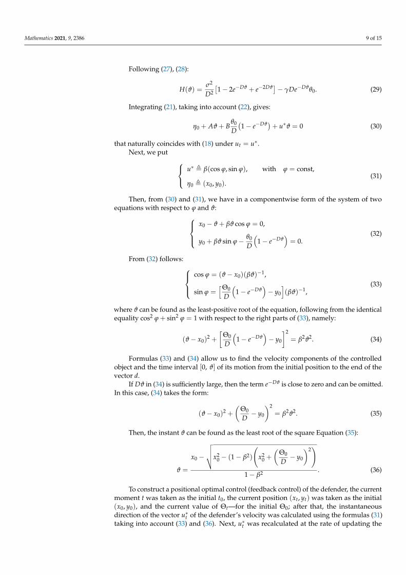
Following (27), (28):
H(ϑ) =σ2
D2
[1− 2e−Dϑ + e−2Dϑ
]− γDe−Dϑθ0. (29)
Integrating (21), taking into account (22), gives:
η0 + Aϑ + Bθ0
D(1− e−Dϑ
)+ u∗ϑ = 0 (30)
that naturally coincides with (18) under ut = u∗.Next, we put u∗ , β(cos ϕ, sin ϕ), with ϕ = const,
η0 , (x0, y0).(31)
Then, from (30) and (31), we have in a componentwise form of the system of twoequations with respect to ϕ and ϑ:
x0 − ϑ + βϑ cos ϕ = 0,
y0 + βϑ sin ϕ− θ0
D
(1− e−Dϑ
)= 0.
(32)
From (32) follows:cos ϕ = (ϑ− x0)(βϑ)−1,
sin ϕ =[Θ0
D
(1− e−Dϑ
)− y0
](βϑ)−1,
(33)
where ϑ can be found as the least-positive root of the equation, following from the identicalequality cos2 ϕ + sin2 ϕ = 1 with respect to the right parts of (33), namely:
(ϑ− x0)2 +
[Θ0
D
(1− e−Dϑ
)− y0
]2= β2ϑ2. (34)
Formulas (33) and (34) allow us to find the velocity components of the controlledobject and the time interval [0, ϑ] of its motion from the initial position to the end of thevector d.
If Dϑ in (34) is sufficiently large, then the term e−Dϑ is close to zero and can be omitted.In this case, (34) takes the form:
(ϑ− x0)2 +
(Θ0
D− y0
)2= β2ϑ2. (35)
Then, the instant ϑ can be found as the least root of the square Equation (35):
ϑ =
x0 −
√√√√x20 − (1− β2)
(x2
0 +
(Θ0
D− y0
)2)
1− β2 . (36)
To construct a positional optimal control (feedback control) of the defender, the currentmoment t was taken as the initial t0, the current position (xt, yt) was taken as the initial(x0, y0), and the current value of Θt—for the initial Θ0; after that, the instantaneousdirection of the vector u∗t of the defender’s velocity was calculated using the formulas (31)taking into account (33) and (36). Next, u∗t was recalculated at the rate of updating the
Mathematics 2021, 9, 2386 10 of 15
current information. Note that at a high rate of updating this information, it may bequite justified to use the piecewise program control of the defender, in which its control isrecalculated only at certain moments called correction moments with intervals betweenthem ∆tu. During these intervals, the defender moves programmatically according tocontrol u∗t , calculated in the previous step.
6. Examples
To demonstrate the effectiveness of the obtained optimal control, a numerical simula-tion was performed for two approaches for studying the interaction between the defenderand SV. These approaches differ in the mathematical description of the evolution of the y-component of the SV’s velocity. In the first (discrete) approach, this component is piecewiseconstant and its evolution is described as a jump-like Markov process θt with three states(1, 0,−1) and the transition intensity matrix Λ from (2). The description of this process isgiven in the beginning of Section 2. In the second (continuous) approach, an evolution ofthe y-component of the SV’s velocity vector is set by Gaussian process Θt, i.e., continuousdiffusion process (3).
In both approaches, the control of the defender was obtained through Equations (31),(33), and (36). In other words, the control of the defender is always calculated according tothe continuous diffusive model (3) of the evolution of the y-component of the SV’s velocityvector. Strictly speaking, as this control law is the result of the solution of the continuousproblem, it should not always successfully solve the discrete problem, simulated in thefirst approach. The idea of these experiments is to apply the solution of the continuousproblem, which can be solved analytically, to the similar discrete practical model, whichcannot be studied in the same convenient way. In all experiments, vector d was consideredto be null, i.e., the defender has to intercept the SV.
Both approaches to the simulation are shown in further examples, which were devotedto two different applications of the studied interception problem.
The realization of diffusive process Θt was acquired in Maple with the package forstochastic equations. An approximate formula for ϑ (36) was used for the stochasticdifferential Equation (15). Thus, Maple allows integrating this equation numerically andobtaining the optimal trajectory of the defender, as well as the random trajectory of theSV corresponding to the process with the appropriate mathematical expectation anddispersion.
A more practical discrete jump-like process θt was simulated in Python script. Themovement of the SV and defender was computed with a very small discretization step∆t, which is the quality of the simulation. At each step, the SV, according to the modelfrom Section 3, can change the direction of its vy velocity component with probability2λ∆t or not change it with probability (1− 2λ∆t). However, in practice, this model is notvery useful. This process is identical to a Gaussian process: the time of another SV tack issampled exponentially with mathematical expectation 1/λ, and the direction of the verticalvelocity for this tack is chosen from two directions, different from the current one withprobability 1/2. The defender, on the other hand, has its own parameter ∆tu and correctsits control law according to (36) every interval ∆tu, considering the current positions tobe initial.
6.1. Intrusion in the Detection Zone
The first application is the intrusion of the SV’s detection zone by the defender todistract the SV from the target. In normalized scale, these parameters are:
R = 1, vx = 1, τo = 0.6.
Let tan α = 0.5. Then, the parameters for Gauss process Θt are:
λ =1τ0≈ 1.67, D = 3λ ≈ 5, σ = 2 tan α
√λ = 1.29.
Mathematics 2021, 9, 2386 11 of 15
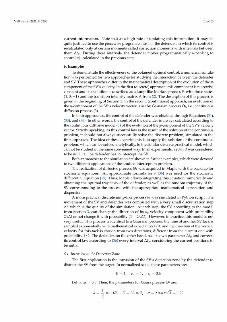
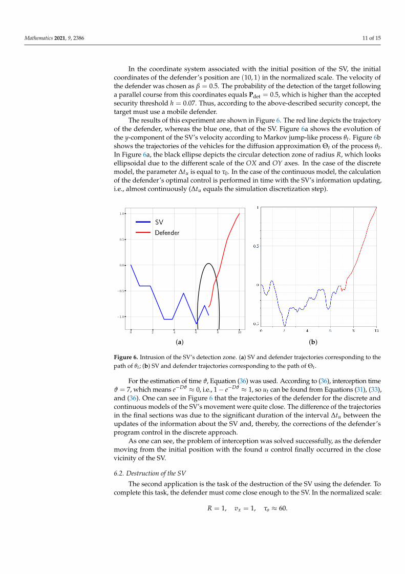
In the coordinate system associated with the initial position of the SV, the initialcoordinates of the defender’s position are (10, 1) in the normalized scale. The velocity ofthe defender was chosen as β = 0.5. The probability of the detection of the target followinga parallel course from this coordinates equals Pdet = 0.5, which is higher than the acceptedsecurity threshold h = 0.07. Thus, according to the above-described security concept, thetarget must use a mobile defender.
The results of this experiment are shown in Figure 6. The red line depicts the trajectoryof the defender, whereas the blue one, that of the SV. Figure 6a shows the evolution ofthe y-component of the SV’s velocity according to Markov jump-like process θt. Figure 6bshows the trajectories of the vehicles for the diffusion approximation Θt of the process θt.In Figure 6a, the black ellipse depicts the circular detection zone of radius R, which looksellipsoidal due to the different scale of the OX and OY axes. In the case of the discretemodel, the parameter ∆tu is equal to τ0. In the case of the continuous model, the calculationof the defender’s optimal control is performed in time with the SV’s information updating,i.e., almost continuously (∆tu equals the simulation discretization step).
0 2 4 6 8 10
−1.0
−0.5
0.0
0.5
1.0
(a) (b)
Figure 6. Intrusion of the SV’s detection zone. (a) SV and defender trajectories corresponding to thepath of θt; (b) SV and defender trajectories corresponding to the path of Θt.
For the estimation of time ϑ, Equation (36) was used. According to (36), interception timeϑ = 7, which means e−Dϑ ≈ 0, i.e., 1− e−Dϑ ≈ 1, so ut can be found from Equations (31), (33),and (36). One can see in Figure 6 that the trajectories of the defender for the discrete andcontinuous models of the SV’s movement were quite close. The difference of the trajectoriesin the final sections was due to the significant duration of the interval ∆tu between theupdates of the information about the SV and, thereby, the corrections of the defender’sprogram control in the discrete approach.
As one can see, the problem of interception was solved successfully, as the defendermoving from the initial position with the found u control finally occurred in the closevicinity of the SV.
6.2. Destruction of the SV
The second application is the task of the destruction of the SV using the defender. Tocomplete this task, the defender must come close enough to the SV. In the normalized scale:
R = 1, vx = 1, τo ≈ 60.

Mathematics 2021, 9, 2386 12 of 15
Let tan α = 0.5. Therefore:
λ = 0.017, D = 0.05, σ = 0.13.
In the coordinate system associated with the initial position of the SV, the initialcoordinates of the defender are (300, 20) in the normalized scale. The velocity of thedefender was chosen as β = 0.5. As the target moves parallel to the general course ofthe SV, then the detection probability Pdet equals Pdet = 0.37 > h = 0.07; thus, using thedefender is justified.
The results of the modeling are presented in Figure 7. As in the first example, Figure 7acorresponds to the discrete approach to the simulation and the process θt, and Figure 7brelates to the continuous approach and the process Θt.
0 50 100 150 200 250 300
−30
−20
−10
0
10
20
(a) (b)
Figure 7. Destruction of the SV. (a) SV and defender trajectories corresponding to the path of θt;(b) SV and defender trajectories corresponding to the path of Θt.
The accuracy of the interception of the SV by the defender or the so-called terminalmiss obviously depends on the parameter ∆tu—the time interval between corrections of thedefender’s control. Figure 8 presents the results of different simulations of the interceptionof the SV by the defender for the discrete approach. Figure 8a corresponds to the case of∆tu = τ0. A sufficient miss of the defender can be explained by the relatively significantduration ∆tu of its movement without control correction and the “inconvenient” realizationof the tack, which combined with the velocity advantage (β < 1) allowed the SV to avoidinterception by the defender. However, decreasing the parameter ∆tu helped achieve moresatisfactory results, as shown in Figure 8b. For two similar realizations of process θt (bluelines), the trajectories of the controlled defender (red lines) were clearly very different withdependence on the parameter ∆tu (τ0 and τ0/10, respectively).

Mathematics 2021, 9, 2386 13 of 15
0 50 100 150 200 250 300
0
5
10
15
20
25
30
35
40
(a) ∆tu = τ0
0 50 100 150 200 250 300
0
5
10
15
20
25
30
35
40
(b) ∆tu = τ0/10
Figure 8. Interception trajectories with different values of ∆tu.
6.3. Comparison with Classic Guidance Methods
The optimal control law of the defender obtained here was compared with classicguidance methods, mentioned in the Introduction, such as the pursuit guidance methodand parallel guidance, which is a specific case of the proportional navigation guidancemethod. On average, our method gave better results than the others. In Figure 9, atypical realization of different simulated guidance methods is presented. The orange linedesignates the trajectory of the defender, acting according to the pursuit guidance method;the red line denotes the trajectory generated by the parallel guidance algorithm; the bluegraph shows the SV’s movement. The defender, controlled according to Equations (31), (33)and (36), has a green trajectory. Dashed lines illustrate the distances on the Y axis betweenthe SV and defender at instant ϑ when their X-coordinates coincide.
Figure 9. Comparison of different guidance methods.
As one can see, the green defender was closer to the SV than the others. Classicguidance methods are effective when the pursuer velocity is higher than the one of theevader. That is not the case in the current study, because the defender’s velocity β was lessthan the velocity of the SV. Moreover, the classic guidance methods are not intended to beuse for intercepting stochastic targets, unlike the control law obtained in this article as asolution of the stochastic optimal control problem.

Mathematics 2021, 9, 2386 14 of 15
7. Conclusions
The article considered one “attacker–target–defender”-type problem of the interactionon a plane between the search system, consisting of one search vehicle with the circledetection zone, and the mobile searched object. The search vehicle tacked randomly alonga given general course towards the searched object, and its movement was describedusing a Markov jump-like process. The searched object had a mobile defender onboard,which can be used for the distraction and destruction of the search vehicle, if it presents adanger to the searched object in the sense of its detection. The feature of this problem isthat the defender has lower dynamic capabilities in comparison to the searching vehiclebeing intercepted.
It was shown that, being stochastic in nature, the optimal control problem of theinterception of a search vehicle can be transformed into the classic deterministic problemof optimal control in the class of piecewise-programmatic controls. The optimal time ofinterception was estimated, and an optimal control law was found. The examples of thenumerical simulations for both the discrete and continuous (stochastic and deterministic)problems were presented to reveal the efficiency of the designed results. Furthermore, acomparison with the interception solutions, based on classic guidance laws, was presented.
In the future, it is planned to consider a similar problem statement with a group ofsearch vehicles instead of one.
Author Contributions: Conceptualization, A.A.G. and E.Y.R.; methodology, A.A.G. and E.Y.R.;software, P.V.L.; validation, A.A.G., P.V.L. and E.Y.R.; formal analysis, A.A.G., P.V.L. and E.Y.R.;investigation, A.A.G. and E.Y.R.; writing—original draft preparation, A.A.G., P.V.L. and E.Y.R.;writing—review and editing, A.A.G., P.V.L. and E.Y.R.; visualization, P.V.L.; supervision, A.A.G. andE.Y.R.; project administration, A.A.G.; funding acquisition, A.A.G. All authors have read and agreedto the published version of the manuscript.
Funding: This paper was partially supported by the Program of Basic Research of RAS.
Institutional Review Board Statement: Not applicable.
Informed Consent Statement: Not applicable.
Data Availability Statement: Data sharing not applicable.
Conflicts of Interest: The authors declare no conflict of interest.
AbbreviationsThe following abbreviations are used in this manuscript:
SO Searched objectSV Search vehicleUAV Unmanned aerial vehicleUUV Unmanned underwater vehicleASV Autonomous surface vehicle
References1. Stone, L.D.; Royset, J.O.; Washburn, A.R. Optimal Search for Moving Targets; Springer International Publishing: Cham, Switzerland,
2016.2. Meghjani, M.; Manjanna, S.; Dudek, G. Multi-target search strategies. In Proceedings of the 2016 IEEE International Symposium
on Safety, Security, and Rescue Robotics (SSRR), Lausanne, Switzerland, 23–27 October 2016; pp. 328–333.3. Youngchul, B. Target searching method in the chaotic mobile robot. In Proceedings of the 23rd Digital Avionics Systems
Conference, Salt Lake City, UT, USA, 24–28 October 2004; Volume 12, pp. 7–12.4. Austin, D.J.; Jensfelt, P. Using multiple Gaussian hypotheses to represent probability distributions for mobile robot localization.
In Proceedings of the 2000 ICRA, Millennium Conference, IEEE International Conference on Robotics and Automation, SanFrancisco, CA, USA, 24–28 April 2000; pp. 1036–1041.
5. Galyaev, A.A.; Lysenko P.V.; Yakhno V.P. Optimal Path Planning for an Object in a Random Search Region. Autom. Remote Control2018, 79, 2080–2089. [CrossRef]
Mathematics 2021, 9, 2386 15 of 15
6. Shaikin, M.E. On statistical risk funstional in a control problem for an object moving in a conflict environment. J. Comput. Syst.Sci. Int. 2011, 1, 22–31.
7. Sysoev, L.P. Criterion of detection probability on trajectory in the problem of object motion control in threat environment. ControlProbl. 2010, 6, 65–72.
8. Andreev, K.V.; Rubinovich, E.Y. Moving observer trajectory control by angular measurements in tracking problem. Autom. RemoteControl 2016, 77, 106–129. [CrossRef]
9. Wettergren, T.A.; Baylog, J.G. Collaborative search planning for multiple vehicles in nonhomogeneous environments. InProceedings of the OCEANS 2009, Biloxi, MS, USA, 26–29 October 2009; pp. 1–7.
10. Wang, Y.; Hussein, I.I. Search and Classification Using Multiple Autonomous Vehicles; Springer: London, UK, 2012.11. Galyaev, A.A.; Maslov, E.P. Optimization of a mobile object evasion laws from detection. J. Comput. Syst. Sci. Int. 2010, 49,
560–569. [CrossRef]12. Galyaev, A.A.; Maslov, E.P. Optimization of the Law of Moving Object Evasion from Detection under Constraints. Autom. Remote
Control 2012, 73, 992–1004. [CrossRef]13. Zabarankin, M.; Uryasev, S.; Pardalos, P. Optimal Risk Path Algorithms Cooperative Control and Optimization; Murphey, P., Ed.;
Kluwer Acad: Dordrecht, The Netherlands, 2002; Volume 66, pp. 271–303.14. Sidhu, H.; Mercer, G.; Sexton, M. Optimal trajectories in a threat environment. J. Battlef. Technol. 2006, 9, 33–39.15. Dogan, A.; Zengin, U. Unmanned Aerial Vehicle Dynamic-Target Pursuit by Using Probabilistic Threat Exposure Map. J. Guid.
Control Dyn. 2006, 29, 723–732. [CrossRef]16. Meyer, Y.; Isaiah, P.; Shima, T. On dubins paths to intercept a moving target. Automatica 2015, 53, 256–263. [CrossRef]17. Zheng, Y.; Chen, Z.; Shao, X.; Zhao, W. Time-optimal guidance for intercepting moving targets by dubins vehicles. Automatica
2021, 128, 109557. [CrossRef]18. Buzikov, M.E.; Galyaev, A.A. Time-minimal interception of a moving target by dubins car. Autom. Remote Control 2021, 82,
745–758. [CrossRef]19. Guelman, M.; Shinar, J. Optimal guidance law in the plane. J. Guid. Control Dyn. 1984, 7, 471–476. [CrossRef]20. Glizer, V.Y. Optimal planar interception with fixed end conditions: Closed-form solution. J. Optim. Theory Appl. 1996, 88, 503–539.
[CrossRef]21. Gopalan, A.; Ratnoo, A.; Ghose, D. Time-optimal guidance for lateral interception of moving targets. J. Guid. Control Dyn. 2016,
39, 510–525. [CrossRef]22. Manyam, S.G.; Casbeer, D.W. Intercepting a target moving on a racetrack path. In Proceedings of the 2020 International Conference
on Unmanned Aircraft Systems (ICUAS), Athens, Greece, 1–4 September 2020; pp. 799–806.23. Siouris, G.M. Missile Guidance and Control Systems; Springer: New York, NY, USA, 2004.24. Lin, C.F. Modern Navigation, Guidance, and Control Processing; Prentice Hall: Hoboken, NJ, USA, 1991.25. Palumbo, N.F.; Blauwkamp, R.; Lloyd, J. Basic Principles of Homing Guidance. Johns Hopkins APL Tech. Digest. 2010 , 29, 25–41.26. Pachter, M.; Garcia, E.; Casbeer, D.W. Active target defense differential game. In Proceedings of the 52nd Annual Allerton
Conference on Communication, Control, and Computing, Monticello, IL, USA, 30 September–3 October 2014; pp. 46–53.27. Pachter, M.; Garcia, E.; Casbeer, D.W. Active Target defense differential game with a fast Defender. In Proceedings of the American
Control Conference (ACC), Chicago, IL, USA, 1–3 July 2015; pp. 3752–3757.28. Zhang, J.; Zhuang, J. Modeling a Multi-target Attacker-defender Game with Multiple Attack Types. Reliab. Eng. Syst. Saf. 2019,
185, 465–475. [CrossRef]29. Galyaev, A.A.; Dobrovidov, A.V.; Lysenko, P.V.; Shaikin, M.E.; Yakhno, V.P. Path Planning in Threat Environment for UUV with
Non-Uniform Radiation Pattern. Sensors 2020, 20, 2076. [CrossRef] [PubMed]30. Krichagina, N.V.; Liptser, R.S.; Rubinovich, E.Y. Kalman filter for Markov processes. In Statistics and Control of Stochastic Processes;
Publ. Div.: New York, NY, USA, 1985; pp. 197–213.31. Ross, I.M. A Primer on Pontryagin’s Principle in Optimal Control; Collegiate Publishers: San Francisco, CA, USA, 2009.