A Probabilistic Scheduler for the Analysis of

Cryptographic Protocols 1

Srecko Brlek∗, Sardaouna Hamadou∗∗, John Mullins∗,∗∗

∗ Lab. LaCIM, Dep. d’Informatique, Universite du Quebec a Montreal.CP 8888 Succursale Centre-Ville, Montreal (Quebec), Canada, H3C 3P8.

∗∗ Lab. CRAC, Dep. de Genie Informatique, Ecole Polytechnique de MontrealP.O. Box 6079, Station Centre-ville, Montreal (Quebec), Canada, H3C 3A7.

Abstract

When modelling cryto-protocols by means of process calculi which express both nondeterministic and prob-abilistic behavior, it is customary to view the scheduler as an intruder. It has been established that thetraditional scheduler needs to be carefully calibrated in order to more accurately reflect the intruder’s capa-bilities for controlling communication channels. We propose such a class of schedulers through a semanticvariant called PPCνσ , of the Probabilistic Poly-time Calculus (PPC) of Mitchell et al. [11] and we illustratethe pertinence of our approach by an extensive study of the Dining Cryptographers (DCP) [8] protocol.Along these lines, we define a new characterization of Mitchell et al.’s observational equivalence [11] moresuited for taking into account any observable trace instead of just a single action as required in the analysisof the DCP.

Keywords: Process algebra, observational equivalence, probabilistic scheduling, analysis of cryptographicprotocols

1 Introduction

Systems that combine both probabilities and nondeterminism are very convenient

for modelling probabilistic security protocols. In order to model such systems, some

efforts have been taken to extend (possibilistic) models based on process algebras

such as either the π-calculus or the CSP, by including probabilities. One can dis-

tinguish two classes of such models. On one hand, we have all purpose probabilistic

models adding probabilities to nondeterministic models [1,6,3]. On the other hand,

we have process algebraic frameworks that define probabilistic models in order to

make them more suitable for applications in security protocols [11,4,10].

While it is customary to use schedulers for resolving non-determinism in proba-

bilistic systems, scheduling processes must be carefully designed in order to reflect

1 Research partially supported by NSERC grants (Canada)

Electronic Notes in Theoretical Computer Science 194 (2007) 61–83

1571-0661/$ – see front matter © 2007 Elsevier B.V. All rights reserved.

www.elsevier.com/locate/entcs

doi:10.1016/j.entcs.2007.10.009

as accurately as possible the intruder’s capabilities for controlling the communica-

tion network without controlling the internal reactions of the system. Consider the

protocol c(a).0|c(b).0 transmitting the messages a and b over c and the intruder

c(x).0 eavesdropping on this channel. As the protocol is purely non deterministic,

the probability of the intercepted message being either a or b should be the same.

A scheduler that could assign an arbitrary probabilistic distribution to these two

messages could also force the protocol to transmit either a or b. Such schedulers

are too strong however, and should therefore not be admissible. But restricting the

power of schedulers should also be carefully done, otherwise this could result in ad-

versaries that are too weak. Forcing schedulers to give priority to internal actions,

for example, makes internal actions completely invisible to attackers. An intruder

is then unable to distinguish a process P from another process which could do some

internal action, and then behaves like P . Consider now the following process:

P = νc′(c(x).c′(x).0|c′(1).0|c′(y).[y = 0]c(secret).0).

In this obviously unsecure protocol, an intruder could send 0 to P over c and thus

allow P to publish the secret. Such a flaw will never be detected in semantics giving

priority to internal actions, since in that case P will never broadcast secret on public

channel c.

Contribution. Our contribution is threefold. Firstly, we define a semantic variant

of the Probabilistic Polynomial-time Process Calculus PPC [11] (Section 2), called

PPCνσ, to cope with the problem of characterizing the intruders’s capacity. Con-

trary to most probabilistic models, our operational semantics does not normalize

probabilities. The reason is that normalizing has the effect of removing control of

its own actions from the intruder. Consider the process P = c(m).Q1|c(m).Q2 :

depending on whether P represents a protocol or an intruder, the scheduling of a

component is respectively equiprobable or arbitrarily chosen by the intruder. A

solution might be to discriminate semantically between a protocol and an intruder,

but this rapidly becomes rather intricate since synchronization actions could be

committed by both. We propose here a simpler solution to this problem. It consists

of equipping the intruder with an attack strategy i.e., a selection process called

external scheduler (Section 2.3), allowing it to choose the next action to perform at

each evaluation step. This scheduling is carefully designed to reflect as accurately

as possible the intruder’s real capacities, i.e. to control the communication network

without controlling internal reactions of the system under its stimuli.

Secondly, we reformulate (Section 3) the observational equivalence of [11] into

a more amenable form to take account of all observable traces instead only single

step.

Finally, to illustrate the pertinence of our approach, we conclude the paper by an

extensive case study (Section 4): the analysis of the Chaum’s Dining Cryptographers

protocol [8]. We give a probabilistic version of the possibilistic specification of

the anonymity property as per Schneider and Sidiropoulos [12], and prove that

restricting the scheduler’s power too much may lead to very weak models which

cannot detect flawed specifications of the protocol.

S. Brlek et al. / Electronic Notes in Theoretical Computer Science 194 (2007) 61–8362

Related work. The technical precursor of our framework is the process calculus

of Mitchell et al. [11]. Though any of the models [1,6,3,11,4,10] or any similar

framework could have been an interesting starting point, the framework of Mitchell

et al. [11] appears appropriate for the following reasons. Although it is a formal

model, it is still close to computational setting of modern cryptography since it

works directly on the cryptographic level. Indeed it defines an extension of the

CCS process algebra with finite replication and probabilistic polynomial-time terms

denoting cryptographic primitives. It turns out that these probabilistic polynomial

functions are useful for modelling the probabilistic behaviour of security systems.

Unlike formalisms such as [6,4,10], the scheduling is probabilistic, better reflecting

so the ability of the attacker to control the communication network. Finally it also

appears as a natural formal framework for capturing and reasoning about a variety

of fundamental cryptographic notions.

The problem of characterizing the schedulers’ capacities has recently been con-

sidered in [5,7,9]. In [5] the authors treated the problem of overly powerful schedulers

in the context of systems modelled in a Probabilistic I/O Automata framework.

They restricted the scheduler by defining two levels of schedulers. A high-level

scheduler called adversarial scheduler is a component of the system and controls

the communication network, i.e. it schedules public channels. This component has

limited knowledge of the behaviour of other components in the system: their in-

ternal choices and secret information are hidden. On the other hand, a low-level

scheduler called tasks scheduler resolves the remaining non-determinism by a task

schedule. These tasks are equivalence classes of actions that are independent of the

high-level scheduler choices. We believe that these tasks may correspond to our

“strategically equivalent action”.

In Garcia et. al. [9] a dual problem to the one we have considered here, namely

the problem that arises when traditional schedulers are overly powerful, is addressed.

In the context of security protocols modelled by probabilistic automata, they define

a probabilistic scheduler that assign, in the current state, a probability distribu-

tion on the possible non-deterministic next transitions. Unlike our scheduler, it is

history-dependent since it defines equiprobable paths and it is not stochastic, and

might therefore halt execution at any time. Roughly speaking, admissible sched-

ulers are defined w.r.t bisimulation equivalence: any observably trace equivalent

paths are equiprobably scheduled and lead to bisimilar states.

Another recent paper on the scheduling issue is presented in [7]. Unlike our

scheduler and that of [9] which are both defined on the semantic level, [7] proposes

a framework in which schedulers are defined and controlled on the syntactic level.

They make random choices in the protocol invisible to the adversary. Note that we

achieve the same goal by using the operational semantics Eval rule which reduces

unblocked processes, as well as our strategically equivalent classes of actions. More

investigation is needed for papers [5,7] to determine how the approaches may benefit

from each other.

Finally an alternate approach is proposed in [4,10]. Instead of scheduling a

single action (like ours), or a path (like the one of [9]), a process is scheduled. The

S. Brlek et al. / Electronic Notes in Theoretical Computer Science 194 (2007) 61–83 63

problems of discriminating between a protocol’s actions and intruder’s ones, and the

privileging of internal actions, is meaningless in these models because scheduling

is included implicitly in the specification. In other words, the protocol designer

determines when control passes from the protocol to the attacker. Let us explain

this last point. Consider the protocol P = ν(c)(c(1).|c(x).c′(0).) which, after an

internal communication, outputs 0 on the public channel c′. In the frameworks of

[4,10], it may be specified in two different manners

P1 = ν(c)(start().c(1).0|c(x).c′(0).0)

and

P2 = ν(c)(start().c(1).0|c(x).contr2Intr().getContr().c′(0).0)

depending on whether or not we want to make the internal action completely in-

visible to the attacker. In this way the user has total freedom and can eliminate

undesirable schedulers at the specification level. The drawback is that the protocol

designer who has incomplete knowledge about the system, may specify his intuition

of the protocol and so get some properties that might not be satisfied by the actual

protocol.

2 The PPCνσ model

The process algebra PPCνσ extends semantically the Probabilistic Polynomial-time

Process Calculus PPC [11] to better take into account the analysis of probabilistic

security protocols.

2.1 Syntax of PPCνσ

Terms. The set of terms T of the process algebra PPCνσ consists of variables V,

numbers N, pairs, and a specific term N standing for the security parameter. The

security parameter may be understood as the cryptographic primitives’ key length

and may appear in the probabilistic polynomial functions defined below. Formally

we have

t ::= n (integer ) | x (variable) | N (secur. param.) | (t, t) (pair )

For each term t, fv(t) is the set of variables in t. A message is a closed term (i.e.

not containing variables). The set of messages is denoted M.

Functions. The call of probabilistic as well as deterministic cryptographic primi-

tives, such as keys and nonces generation, encryption, decryption, etc., is modelled

by probabilistic polynomial functions 2 Λ : Mk → M satisfying

∀(m1, . . . ,mk) ∈ Mk, ∀m ∈ M, ∀λ ∈ Λ, ∃p ∈ [0, 1] such that

Prob[λ(m1, · · · ,mk) = m] = p.

We denote λ(m1, · · · ,mk) ↪→ x the assignment of the value λ(m1, · · · ,mk) to

the variable x and by λ(m1, · · · ,mk)p

↪→ m if λ(m1, · · · ,mk) evaluates to m with

2 See Appendix A for a formal definition of a probabilistic polynomial function

S. Brlek et al. / Electronic Notes in Theoretical Computer Science 194 (2007) 61–8364

probability p. From Definition A.1 (see Appendix A), the set

Im(λ(m1, · · · ,mk)) = {m | ∃p ∈]0..1] λ(m1, · · · ,mk)p

↪→ m}

of m s.t. λ(m1, · · · ,mk) evaluates to m with non-zero probability, is a finite set.

For instance, RSA encryption which takes as parameters, a message m to encrypt

and an encryption key formed of the pair (e, n), and returns the number me mod n,

is the function λRSA(m, e, n) returning c with probability 1 if c = me mod n, and

0 otherwise. Similarly, we can model the key guessing attack of a cryptosystem by

the product [rand(1k) ↪→ key][dec(c, key) ↪→ x] where 1k is the size of the key

randomly generated by the function rand, and the decryption function dec returns

m with probability 1 if c is the cryptogram of m encrypted by k and key = k. The

success of such an attack has probability p = 12|k|

. These few examples illustrate the

expressive power offered by these functions. We limit ourselves to the probabilistic

polynomial ones in order to model all attacks realizable (in the model) in polynomial

time.

Processes. Let C be a countable set of public channels. We assume that each

channel is equipped with a bandwidth given by the polynomial function bw : C −→N. We say that a message m belongs to the domain of a channel c, written m ∈dom(c), if the message length |m| is less than or equal to the channel bandwidth,

i.e. m ∈ dom(c) ⇐⇒ |m| ≤ bw(c). Note that |(m,m′)| = |m| + |m′| + r where r

is the length of a fixed bits string, which allows us to concatenate and decompose

two terms without any ambiguity.

Processes in PPCνσ are built as follows :

P ::= 0 | c(x).P | c(m).P | P |P | (νc)P | [t = t]P |

| !q(N)P | [λ(t1, · · · , tn) ↪→ x]P

Given a process P , the set fv(P ) of free variables, is the set of variables x in P which

are not in the scope of any prefix either input (of the form c(x)) or probabilistic

evaluation (of the form [λ(t1, · · · , tn) ↪→ x]). A process without free variables

is called closed and the set of closed processes is denoted by Proc. Hereafter, all

processes are considered closed.

The mechanisms for reading, emitting, parallel composition, restriction and mat-

ching are all standard. The finite replication !q(N)P is the q(N)−fold parallel com-

position of P with itself, where q is a polynomial function. The novelty is the call

and return of probabilistic polynomial functions

[λ(t1, · · · , tn) ↪→ x]P

This feature allows to model (probabilistic) polynomial cryptographic primitives as

well as the probabilistic character of a protocol. In fact it is the main source of

probability in this model.

The following examples illustrate the way PPCνσ can be used to model protocols.

Example 2.1 Let Kgen be a (probabilistic) polynomial function that, given the

security parameter N, generates a secret encryption key and enc a (probabilistic)

S. Brlek et al. / Electronic Notes in Theoretical Computer Science 194 (2007) 61–83 65

encryption function that, given a secret key K and a message M , returns the cryp-

togram of M under K. The process P that receives a message over the public

channel c generates an encryption key and returns the cryptogram of this message

over the same public channel. This is modeled in PPCνσ as follows:

P := c(x).[Kgen(N) ↪→ y][enc(x, y) ↪→ z]c(z).0

Example 2.2 Though that the calculus does not consider the probabilistic alter-

native choice operator “+”, it is possible to simulate it by means of the parallel

composition operator and some special probabilistic functions.

Let flips be a probabilistic polynomial function that given a coin return Head

with probability p and Tail with probability 1− p. Then the process Q that flips a

coin and then behaves as the process Q′ if the result of coin flipping is Head and

as the process Q′′ otherwise, is modeled in our calculus as follows:

Q := [flips(coin) ↪→ x]([x = Head]Q′|[x = Tail]Q′′)

2.2 Operational semantics

The set of actions

Act = {c(m), c(m), c(m) · c(m), c(m) · c(m), τ | m ∈ M and c ∈ C}

consists of the set of partial input and output actions, of the set of synchronization

actions on public channels, and of the internal action τ :

Partial = {c(m), c(m) | m ∈ M and c ∈ C}

Actual = {c(m) · c(m), c(m) · c(m), τ | m ∈ M and c ∈ C}

The set of observable actions is given by Vis = Act−{τ}. The operational semantics

of PPCνσ is a probabilistic transition system (E ,T , E0) generated by the inference

rules given in Table 1 where E ⊆ Proc is the set of states, T ⊆ E × Act × [0, 1] × E

the set of transitions and E0 ∈ Proc the initial state. The notation Pα[p]−→P ′ stands

for (P,α, p, P ′) ∈ T . It is an extension of the CCS semantics, with a mechanism for

calling probabilistic polynomial functions. We sketch it briefly here.

To make sure that internal computations of functions do not interfere with com-

munication actions (in particular with those on public channels controlled by the

intruder), all exposed functions in a process (Eval rule) are simultaneously eval-

uated by the probabilistic polynomial function eval defined in Table 2 below as

illustrated in Example 2.3. This evaluation step allows us to get what we call a

blocked process, i.e. a process having no more internal computations to perform.

The set of blocked processes is denoted by Blocked .

Example 2.3 If processes Q′ and Q′′ of Example 2.2 are blocked processes then Q

reduces to Q′ with probability p and to Q′′ with probability 1 − p. In other words,

Prob[eval(Q) = Q′] = p and Prob[eval (Q) = Q′′] = 1 − p.

The output mechanism allows a principal A to send a message on public channels

(Output rule). Dually, the input mechanism must be ready to receive any message

S. Brlek et al. / Electronic Notes in Theoretical Computer Science 194 (2007) 61–8366

Eval.eval(P )

p↪→P ′ P �∈Blocked

Pτ [p]−→P ′

Outputm ∈ dom(c)

c(m).Pc(m)[1]−→ P

ParL.P1

α[p]−→P ′

1 (P1|P2)∈Blocked

P1|P2

α[p]−→P ′

1|P2

SyncL.P1

c(m)[p1]−→ P ′

1 P2

c(m)[p2]−→ P ′

2

P1|P2

c(m).c(m)[p1.p2]−→ P ′

1|P′2

RestCL.P

c(m).c(m)[p]−→ P ′

(νc)Pτ [p]−→(νc)P ′

Inputm ∈ dom(c)

c(x).Pc(m)[1]−→ P [m/x]

ParR.P2

α[p]−→P ′

2 (P1|P2)∈Blocked

P1|P2

α[p]−→P1|P ′

2

SyncR.P1

c(m)[p1]−→ P ′

1 P2

c(m)[p2]−→ P ′

2

P1|P2

c(m).c(m)[p1.p2]−→ P ′

1|P′2

RestCR.P

c(m).c(m)[p]−→ P ′

(νc)Pτ [p]−→(νc)P ′

RestP

α[p]−→P ′ α�∈{c(m),c(m),c(m)·c(m),c(m)·c(m):m∈M} P∈Blocked

(νc)Pα[p]−→(νc)P ′

Table 1Operational semantics of PPCνσ

Prob[eval(0) = 0] = 1

Prob[eval(c(x).P ) = c(x).P ] = 1 and Prob[eval(c(m).P ) = c(m).P ] = 1

Prob[eval((νc)P ) = (νc)Q] = Prob[eval(P ) = Q](Prob[eval([m = m′]P ) = Q] = Prob[eval(P ) = Q] if m = m′

Prob[eval([m = m′]P ) = 0] = 1 else

Prob[eval(P |Q) = P ′|Q′] = Prob[eval(P ) = P ′] × Prob[eval(Q) = Q′]

Prob[eval([λ(m1, · · · , mk) ↪→ x]P ) = Q] =Pm∈Im(λ(m1,··· ,mk)) Prob[λ(m1, · · · , mk) = m] × Prob[eval(P [m/x]) = Q]

Table 2Reduction of unblocked processes

on a public channel (Input rule). The parallelism (Par. rules) operator is defined

as usual. It is worth noting that the semantics keep track of information involved in

an interaction (the message and the communication channel) (Syn. rules), contrary

to most process algebra semantics where this information is lost, as the only action

resulting from such a communication is usually the invisible action τ . The restriction

operator ν is used to model private channels. The process (νc)P behaves like P

restricted to actions not on c unless a synchronization occurs on c (i.e. actions of

the form c(m) · c(m) or c(m) · c(m)). In this case, they are observed as an invisible

action τ (Rest. rules).

Note that, transition systems generated by the operational semantics (Table 1)

of PPCνσ processes, are not purely probabilistic. Consider for example process P =

c1(a)|c2(b). Clearly, the sum of probabilities of outgoing transitions of P , is equal

to 2. This is due to the parallel composition which introduces nondeterminism. In

order to resolve this nondeterminism it is mandatory to schedule, at each evaluation

step of the process, all available distinct actions. However, security protocols are

assumed to be executed in hostile environments, i.e. environments with external

intruders having full control of the communication network, with the ability to assign

any probabilistic distribution to the controlled channels (to the public actions). This

S. Brlek et al. / Electronic Notes in Theoretical Computer Science 194 (2007) 61–83 67

is modelled by putting public actions under control of an external scheduler. Since

we do not want to define a particular attack strategy, the scheduling is not included

in the semantics of processes, but rather in the intruder’s definition: the intruder

is then formed by the pair (Π, S) of process Π and scheduler S. One may view the

hostile environment as Π interacting with the protocol, and S as its attack strategy.

2.3 External Scheduler

Given a protocol P attacked by the intruder (Π, S), evaluation of P |Π along the

strategy S is a four step process consisting of:

Reduction: evaluation of all exposed probabilistic functions in P |Π.

Localization: indexing of executable actions along eval(P |Π) to discriminate whether

or not an executable action interferes with an intruder’s action.

Selection: scheduling 3 S among available actions.

Execution: the action chosen by S is executed and the process is repeated until

there are no more executable actions.

Localization. Scheduling should be capable of determining whether or not the in-

truder is attached to an action. Since a system P attacked by the intruder Π is

simply modelled by P |Π, actions are indexed by the positions of the components

they belong to, e.g. if P and Π have respectively n and k parallel components, then

P |Π consists of n + k components. By convention the attacker is on the right side,

so that actions indexed by integers less than or equal to n belong to the protocol

while those indexed by integers greater than n belong to the intruder. A partial

action is indexed with an integer denoting the component to which it belongs, while

a communication action is indexed by a pair of integers denoting the components

to which complementary partial actions belong.

Let Index = N∪N2 and the function support : Act \ {τ} → C where support(α)

is the name of the channel where α occurred.

Definition 2.4 The localization function χ : Blocked −→ 2Act×Index is definedrecursively as follows:

χ(0) = ∅

χ(α.P ) = {(α, 1)}

χ(P |Q) = χ(P ) ∪ {(α, ρ(P ) + i) | (α, i) ∈ χ(Q)}

∪{(α · α, i, ρ(P ) + j) | (α, i) ∈ χ(Q) and (α, j) ∈ χ(Q)}

χ((νc)P ) = {(τ, i, j) | (α · α, i, j) ∈ χ(P ) and support(α) = c}

∪{(τ, k, l) | (τ, k, l) ∈ χ(P )}

where α ∈ Partial , max(i, (j, k)) = max(i, j, k). and

ρ(P ) =

(max{ID ∈ Index | (β, ID) ∈ χ(P ), β ∈ Vis} if χ(P ) �= ∅

0 otherwise

3 Note that scheduling is defined only for blocked processes. In fact, the only action available to anunblocked process is the internal action corresponding to functions evaluation.

S. Brlek et al. / Electronic Notes in Theoretical Computer Science 194 (2007) 61–8368

Selection. The function χ allows for action localization, but more guidelines are

needed to know whether or not an indexed action interferes with an intruder’s com-

ponents. Actually, a partition of the set of indexed actions into classes of strategi-

cally equiprobable actions, i.e. classes of actions uniformly chosen in a strategy S, is

needed. Intuitively, a class corresponds to actions which can not be distinguished by

any scheduler. The construction of the quotient set must agree with the following

principles:

(1) No strategy distinguishes between internal actions of a protocol.

(2) No strategy allows the intruder to control internal reactions of a protocol P to

any external stimulus. So, if P can react in many positions to a stimulus of

the intruder, then all these positions should have the same probability to react

to the intruder’s request.

(3) In any strategy, the intruder has complete control on its own actions.

Given a protocol P and an attacker Π, we use χ to compute two sets I1 and I2s.t. indices corresponding to the protocol’s components belong to I1 and thosecorresponding to the intruder’s ones belong to I2. Formally:

I1 =

({1, 2, · · · , ρ(eval(P ))} if χ(eval(P )) �= ∅

∅ otherwise

I2 =

({ρ(eval(P )) + 1, · · · , ρ(eval(P )) + ρ(eval(Π))} if χ(eval(Π)) �= ∅

∅ otherwise

Example 2.5 Let P = c(m).P1|c(m′).P2 et Π = c(x).Π′ then χ(eval(P |Π)) is the

set

{(c(m), 1), (c(m′), 2), (c(m), 3), (c(m′), 3), (c(m) · c(m), 1, 3), (c(m′) · c(m′), 2, 3)}

and so, I1 = {1, 2} et I2 = {3}.

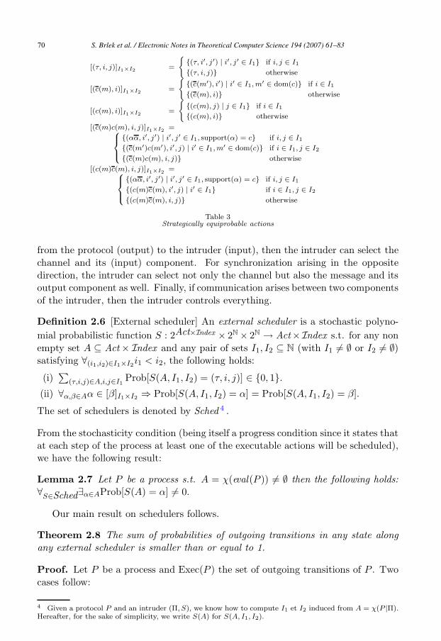
The quotient set of strategically equiprobable actions is summarized in Table 3

where [(α, ID)]I1×I2 denotes the equiprobable class of the indexed action (α, ID)

w.r.t. sets I1 and I2. Let us briefly describe these classes.

Due to principle (1), internal actions of P are equiprobable: it is reflected in

the definition of [(τ, i, j)]I1×I2; τ actions indexed by the components positions of

P (i.e. in I1) are equivalent. Otherwise [(τ, i, j)]I1×I2 is reduced to itself w.r.t (3).

Due to principle (2), partial outputs on a given public channel are equiprobable:

although the intruder can choose the public channel to spy on, it has no control

of messages transmitted on it. Otherwise [(c(m), i)] is reduced to itself: being an

intruder’s action, it can choose both the message and the component to build its

attack. Partial input is the dual case of partial output, with, by contrast, the

intruder controlling the message (sent by itself) that is received by P . The same

principles apply to public synchronization. The intruder can choose a listening

channel c and act merely as an observer, then any communication on c takes place

between two components of P . It has no control on either the messages exchanged,

nor on components where communication occurs. However, if communication arises

S. Brlek et al. / Electronic Notes in Theoretical Computer Science 194 (2007) 61–83 69

[(τ, i, j)]I1×I2 =

({(τ, i′, j′) | i′, j′ ∈ I1} if i, j ∈ I1

{(τ, i, j)} otherwise

[(c(m), i)]I1×I2 =

({(c(m′), i′) | i′ ∈ I1, m′ ∈ dom(c)} if i ∈ I1

{(c(m), i)} otherwise

[(c(m), i)]I1×I2 =

({(c(m), j) | j ∈ I1} if i ∈ I1

{(c(m), i)} otherwise

[(c(m)c(m), i, j)]I1×I2 =8><>:

{(αα, i′, j′) | i′, j′ ∈ I1, support(α) = c} if i, j ∈ I1

{(c(m′)c(m′), i′, j) | i′ ∈ I1, m′ ∈ dom(c)} if i ∈ I1, j ∈ I2

{(c(m)c(m), i, j)} otherwise

[(c(m)c(m), i, j)]I1×I2 =8><>:

{(αα, i′, j′) | i′, j′ ∈ I1, support(α) = c} if i, j ∈ I1

{(c(m)c(m), i′, j) | i′ ∈ I1} if i ∈ I1, j ∈ I2

{(c(m)c(m), i, j)} otherwise

Table 3Strategically equiprobable actions

from the protocol (output) to the intruder (input), then the intruder can select the

channel and its (input) component. For synchronization arising in the opposite

direction, the intruder can select not only the channel but also the message and its

output component as well. Finally, if communication arises between two components

of the intruder, then the intruder controls everything.

Definition 2.6 [External scheduler] An external scheduler is a stochastic polyno-

mial probabilistic function S : 2Act×Index × 2N × 2N → Act×Index s.t. for any non

empty set A ⊆ Act × Index and any pair of sets I1, I2 ⊆ N (with I1 �= ∅ or I2 �= ∅)satisfying ∀(i1,i2)∈I1×I2i1 < i2, the following holds:

(i)∑

(τ,i,j)∈A,i,j∈I1Prob[S(A, I1, I2) = (τ, i, j)] ∈ {0, 1}.

(ii) ∀α,β∈Aα ∈ [β]I1×I2 ⇒ Prob[S(A, I1, I2) = α] = Prob[S(A, I1, I2) = β].

The set of schedulers is denoted by Sched 4 .

From the stochasticity condition (being itself a progress condition since it states that

at each step of the process at least one of the executable actions will be scheduled),

we have the following result:

Lemma 2.7 Let P be a process s.t. A = χ(eval(P )) �= ∅ then the following holds:

∀S∈Sched∃α∈AProb[S(A) = α] �= 0.

Our main result on schedulers follows.

Theorem 2.8 The sum of probabilities of outgoing transitions in any state along

any external scheduler is smaller than or equal to 1.

Proof. Let P be a process and Exec(P ) the set of outgoing transitions of P . Two

cases follow:

4 Given a protocol P and an intruder (Π, S), we know how to compute I1 et I2 induced from A = χ(P |Π).Hereafter, for the sake of simplicity, we write S(A) for S(A, I1, I2).

S. Brlek et al. / Electronic Notes in Theoretical Computer Science 194 (2007) 61–8370

[P �∈ Blocked ]: in this case there is no scheduling and

Exec(P ) = {Pτ [q]−→Q | eval(P)

q↪→ Q}.

The sum of the probabilities of outgoing transitions of P is

p =∑

Q∈Im(eval(P))

Prob[eval(P) = Q]

≤ 1 by definition of eval .

[P ∈ Blocked ]: in this case:

Exec(P ) = {tID = Pα[qID]−→ Q | (α, ID) ∈ χ(P )}.

The sum of the probabilities of outgoing transitions of P according to the scheduler

S is

p =∑

(α,ID)∈χ(P )

Prob[S(χ(P )) = (α, ID)] × qID

≤∑

(α,ID)∈χ(P )

Prob[S(χ(P )) = (α, ID)] since ∀ID ∈ Index , qID ≤ 1

≤ 1 by definition of S.

�

2.4 Cumulative probability distribution

Transition systems induced by the operational semantics of Table 1 may have a

state P with several outgoing transitions labeled by the same action and the same

probability. But to correctly compute the probability of outgoing transitions of P

according to a scheduler, we must ensure that they can be uniquely identified. If

P is blocked then χ enables us to uniquely index the outgoing transitions of P . If

P is unblocked then there exists a finite number n = |Im(eval(P ))| of processes Qi

(1 ≤ i ≤ n) s.t. ∃qi �=0 Pτ [qi]−→Qi is an outgoing transition of P . We can order Qi from

1 to n and use this ordering to index outgoing transitions of P s.t. Pτ [qi]−→Qi being

indexed by (i, i) 5 .

Let σ = (α1, id1) . . . (αn, idn) be a sequence of indexed actions. Then σ is a path

from P to Q if there exist nonzero probabilities p1, . . . , pn s.t.

P0α1[p1]−→ P1

α2[p2]−→ · · ·

αn[pn]−→ Pn,

P = P0 and Q = Pn. Similarly, we say that P reaches Q by path σ with probability

p according to S, denoted by Pσ[p]=⇒S Q, if the probability that S chooses σ is

Prob[S(σ)] =∏

1≤i≤n qi = p where

5 by analogy to the indexing of τ actions by χ

S. Brlek et al. / Electronic Notes in Theoretical Computer Science 194 (2007) 61–83 71

qi =

⎧⎨⎩

pi if Pi−1 �∈ Blocked

Prob[S(χ(Pi−1)) = (αi, idi)] × pi otherwise

Example 2.9 Let P be the process whose transition system in shown in Figure 1

where P1 �∈ Blocked and Prob[eval (P1) = Pi] = pi for 3 ≤ i ≤ 5. Let S be scheduler

such that

• Prob[S({(α1, 1); (α2, 2)}) = (α1, 1)] = q

• Prob[S({(α1, 1); (α2, 2)}) = (α2, 2)] = 1 − q 6

• Prob[S({(α3, 1)}) = (α3, 1)] = 1 (according to the stochasticity condition).

��

��

���� �

P4

P3

P5

P1

P

Q��

��

��

���

α2[p2]

α1[p1]

τ [p3]τ [p4]

τ [p5]

α3[p6]

P2

��

��

���

��

���

����

Fig. 1. Transition system of P

Then the probability that P reaches Q by the path σ = (α1, 1)(τ, (2, 2))(α3 , 1)

according to the scheduler S is

Prob[S(σ)] = (p1 × q) × p4 × (p6 × 1).

An α-path is a path of type (τ, id1)(τ, id2) . . . (τ, idn−1)(α, idn) (n ≥ 1). The

notation Pα[p]=⇒S Q means that there exists an α-path σ s.t. P

σ[p]=⇒S Q. Similarly

Pα[p]=⇒S Q denotes P

α[p]=⇒S Q if α �= τ and P

τ∗[p]=⇒S Q otherwise.

Let E ⊆ Proc be a set of processes and Q ∈ E . Let P be a process, and σ an

α-path from P to Q. Then σ is minimal w.r.t E if no other α-path σ′ exists from

P to Q′ s.t. σ′ is a prefix 7 of σ and Q′ ∈ E . We denote by Paths(P,α

=⇒,E ) the set

of all minimal α-paths from P to an element of E .

Definition 2.10 Let E ⊆ Proc be a set of processes. The cumulative probabilitythat P reaches a process in E by an α-path according to S is computed by thecumulative probability function μ : Proc × Act × 2Proc × Sched → [0, 1]

μ(P,α

=⇒S , E ) =

(1 if P ∈ E , α = τP

{Prob[S(σ)] : σ ∈ Paths(P,α

=⇒, E )} otherwise

The next theorem follows by induction on the length of α-paths.

Theorem 2.11 The cumulative probability function is well defined i.e.

∀P,α,E ,S μ(P,α

=⇒S ,E ) ≤ 1.

6 Note that if (α1, 1) and (α2, 2) are equiprobable then q = 1 − q, i.e. q = 12.

7 Prefixing does not take into account any indexing, e.g. (α1, id3) is a prefix of (α1, id1)(α2, id2) for allindex id1 and id3. Note also that the minimality condition applies only to τ -paths.

S. Brlek et al. / Electronic Notes in Theoretical Computer Science 194 (2007) 61–8372

3 Probabilistic behavioural equivalences

Now we plan to establish equivalences ensuring that a protocol satisfies a security

property if and only if it is observationally equivalent to an abstraction of the

protocol, satisfying the security property by construction. In other words we request

two processes to be equivalent if and only if, when subject to same attacks, they

generate “approximately” the same observations. By “approximately” we mean

asymptotically closed w.r.t. the security parameter 8 .

3.1 Asymptotic observational equivalence

We start by defining the notion of an observable and the probability that a given

process P generates a particular observable. An observable is simply a pair (c,m) of

a public channel and a message. The set of all observables is denoted by Obs. The

probability of observing (c,m) is defined as the sum of the probability of observing

it directly, i.e. the cumulative probability of executing an c(m) · c(m)-path or an

c(m) · c(m)-path to reach any state, and the probability of observing it indirectly,

i.e. by observing first some different visible actions before observing it. For that

purpose we extend the notion of cumulative probability to the so-called cumulative

probability up to H.

Definition 3.1 Let E ⊆ Proc be a set of processes, P a process, S a scheduler andH ⊂ Actual \ {τ} a set of visible actions. The cumulative probability up to H isdefined inductively as follows: ∀α ∈ Actual \ H

μ(P,α

=⇒S/H , E ) =

8>><>>:

1 if P ∈ E and α = τ,

μ(P,α

=⇒S , E )+Pβ∈H, Q∈Proc

μ(P,β

=⇒S , {Q})μ(Q,α

=⇒S/H , E ) otherwise

Lemma 3.2 The cumulative probability up to H is well defined, i.e. ∀P,α,E , S

and H, μ(P,α

=⇒S/H ,E ) ≤ 1.

Proof. If P ∈ E and α = τ , then μ(P,α

=⇒S/H ,E ) = 1 and the result follows.

Assume that we are not in that case. Let σ = τ∗α1 · · · τ∗αn be a path of n actual

visible actions separated by finite numbers of internal actions (we omit the index of

the actions). We say that action αi (1 ≤ i ≤ n) is at distance i from process P on

path σ according to the scheduler S, denoted dσ(P,αi, S) = i, if there exist both a

nonzero probability p, and a process Q such that Pσ[p]=⇒S Q and ∀j < i αj �= αi.

In other words, dσ(P,α, S) is the first position of the visible action α on path σ.

Similarly, let α �∈ H be an actual visible action and

ΣH(α) = {σ = τ∗α1τ∗α2 · · · τ

∗αnτ∗α | n ∈ N and ∀i ≤ n, αi ∈ H}.

Then α is at maximal distance k w.r.t H from the process P according to the

scheduler S, denoted by dH(P,α, S) = k, if supσ∈ΣH(α) dσ(P,α, S) = k. To prove

8 For verification purpose, all along this section, we consider only actual actions (i.e. actions in Actual)keeping in mind that partial actions are never executable. So far partial actions have been considered purelyfor the sake of semantic soundness and completeness.

S. Brlek et al. / Electronic Notes in Theoretical Computer Science 194 (2007) 61–83 73

the claim, we proceed by induction on dH(P,α, S). Let α ∈ Actual \ (H ∪{τ}). We

have:

[Basis] if dH(P,α, S) = 0 then

μ(P,α

=⇒S/H ,E ) = μ(P,α

=⇒S ,E ) ≤ 1.

[Inductive step] Assume that the claim holds for all Q s.t. dH(Q,α, S) < n.

Since

μ(P,α

=⇒S/H ,E ) = μ(P,α

=⇒S,E )

+∑

β∈H, Q∈Proc

μ(P,β

=⇒S , {Q})μ(Q,α

=⇒S/H ,E )

and by induction hypothesis, μ(Q,α

=⇒S/H ,E ) ≤ 1, it remains to show that

μ(P,α

=⇒S,E ) +∑

β∈H, Q∈Proc

μ(P,β

=⇒S , {Q}) ≤ 1,

But we have

μ(P,α

=⇒S ,E ) +∑

β∈H, Q∈Proc

μ(P,β

=⇒S , {Q})

≤∑

β∈H∪{α}

μ(P,β

=⇒S ,Proc)

But that sum is smaller than the sum of the probabilities of outgoing transitions

from the state P according to scheduler S, which is less than or equal to 1 according

to the Theorem 2.8. �

Definition 3.3 Let o = (c,m) be an observable and Lo = {c(m)·c(m), c(m)·c(m)}.The cumulative probability that P generates o according to S is

Prob[P �S o] =∑α∈Lo

μ(P,α

=⇒S/(Actual\(Lo∪{τ})),Proc).

Lemma 3.4 The cumulative probability of an observable is well defined, i.e. ∀P, o,

and S, Prob[P �S o] ≤ 1.

Proof. The proof is given in Appendix B. �

We define our asymptotic observational equivalence relation as stating that two

processes are equivalent if they generate the same observables with approximately

the same probabilities when they are attacked by the same enemy.

Definition 3.5 Let Poly : N → R+ be the set of positive polynomials and E =

Proc × Sched the set of attackers. Two processes P and Q are observationally

equivalent, written P � Q, iff ∀q∈Poly, ∀o∈Obs , ∀(Π,S)∈E , ∃i0 s.t. ∀N≥i0

|Prob[P |Π �S o] − Prob[Q|Π �S o]| ≤1

q(N)

S. Brlek et al. / Electronic Notes in Theoretical Computer Science 194 (2007) 61–8374

Theorem 3.6 The observational relation � is an equivalence relation.

Proof. Reflexivity and symmetry are obvious. For transitivity, let P , Q and R be

processes such that P � Q and Q � R. Let q be a polynomial, o an observation

and (Π, S) an attacker. Then P � Q ⇒ ∃i0 such that ∀N ≥ i0

|Prob[P |Π �S o] − Prob[Q|Π �S o]| ≤1

2q(N),

and Q � R ⇒ ∃j0 such that ∀N ≥ j0

|Prob[Q|Π �S o] − Prob[R|Π �S o]| ≤1

2q(N).

It follows that ∀N ≥ k0 = max(i0, j0) we have

|Prob[P |Π �S o] − Prob[R|Π �S o]|

= |Prob[P |Π �S o]−Prob[Q|Π �S o]

+ Prob[Q|Π �S o] − Prob[R|Π �S o]|

≤ |Prob[P |Π �S o]−Prob[Q|Π �S o]|

+ |Prob[Q|Π �S o] − Prob[R|Π �S o]|

≤1

2q(N)+

1

2q(N)=

1

q(N).

�

In order to develop methods for reasoning about security properties of crypto-

protocols based on observable traces, we reformulate the observational equivalence

to take into account any observable trace.

3.2 Trace equivalence

We start by defining the cumulative probability that a process P generates a se-

quence of observables o1o2 · · · on recursively as the probability that the process di-

rectly generates o1 and reaches a state Q, times the cumulative probability that the

process Q generates the remaining sequence.

Definition 3.7 Let o1o2 · · · on be a sequence of observables s.t. ∀i ≤ n, oi = (ci,mi)

and P be a process. Let αi = ci(mi) · ci(mi) and βi = ci(mi) · ci(mi) ∀1 ≤ i ≤ n.

The cumulative probability that P generates the sequence o1o2 · · · on according to

scheduler S is

Prob[ P �trS o1o2 · · · on]

=∑

Q∈Proc

(μ(P,α1=⇒S, {Q}) + μ(P,

β1=⇒S , {Q}))Prob[Q �

trS o2 · · · on].

Lemma 3.8 The cumulative probability of observing a sequence of observables is

well defined, i.e. ∀P, o1, o2, · · · , on and S, Prob[P �trS o1o2 · · · on] ≤ 1.

Proof. It follows easily by induction on the length of sequences and from Lemma 3.2

and Theorem 2.8. �

S. Brlek et al. / Electronic Notes in Theoretical Computer Science 194 (2007) 61–83 75

Definition 3.9 Two processes P and Q are trace equivalent, as denoted by P �tr

Q, iff ∀q∈Poly, ∀o1,o2,··· ,on∈Obs , ∀(Π,S)∈E , ∃i0 s.t. ∀N≥i0

|Prob[P |Π �trS o1o2 · · · on] − Prob[Q|Π �

trS o1o2 · · · on]| ≤

1

q(N)

Theorem 3.10 �tr is an equivalence relation.

Proof. Similar to the proof of Theorem 3.6. �

To conclude this section we have the following important result that relates the

two equivalence relations.

Theorem 3.11 Trace and observational equivalences are equivalent, i.e.

∀P,Q∈ProcP �tr Q ⇔ P � Q.

Proof. The proof is given in Appendix B. �

4 Case study: the Dining Cryptographers protocol

The Dining Cryptographers [8] protocol is a paradigmatic example of a protocol

which ensures anonymity. Its author defines it as follows:

Three cryptographers are sitting down to dinner at their favorite restaurant. Their

waiter informs them that arrangements have been made with the maitre d’hotel

for the bill to be paid anonymously. One of the cryptographers might be paying

for the dinner, or it might have been NSA (U.S. National Security Agency). The

three cryptographers respect each other’s right to make an anonymous payment,

but they wonder if NSA is paying.

To fairly resolve their uncertainty, they carry out the following protocol: each

cryptographer flips a coin between himself and the cryptographer on his right, so

that only the two of them can see the outcome. Each one of them then states

whether or not the two coins he can see fell on the same side. The payer (if any!)

states the opposite of what he sees. The idea is that if the coins are unbiased and

the protocol is carried out faithfully then an odd number of “different” indicates

that one of them is paying and neither of the other two learns anything about his

identity; otherwise NSA is paying.

4.1 A flawed specification of the protocol

In the following specification 9 we suppose that the NSA makes his choice accordingto a probabilistic distribution (known only to himself) defined by the function λNSAand informs each cryptographer over a secure channel if whether or not he is thepayer. To ensure fairness between cryptographers, i.e. no one having advantageover another, each flip of a coin is made by an “outside trusted third party” by

9 where ⊕ is the addition modulus 2.

S. Brlek et al. / Electronic Notes in Theoretical Computer Science 194 (2007) 61–8376

means of the function flips and the result is made available to both concernedcryptographers.

NSA ::= [λNSA(3) ↪→ x](Y

0≤i≤3

[x = i]Payeri)

Payer3 ::= c0(nopay).c1(nopay).c2(nopay).0

Payeri ::= ci(pay).ci⊕1(nopay).ci⊕2(nopay).0 if 0 ≤ i ≤ 2.

Crypts ::= [flips(coin0) ↪→ y0][flips(coin1) ↪→ y1][flips(coin2) ↪→ y2]Y

0≤i≤2

Crypti

Crypti ::= ci(zi).([zi = pay]Pi|[zi = nopay]Qi)

Pi ::= [yi = yi⊕1]pubi(desagree).0|[yi �= yi⊕1]pubi(agree).0

Qi ::= [yi = yi⊕1]pubi(agree).0|[yi �= yi⊕1]pubi(desagree).0

The protocol is then specified as follows: DCP 1 ::= νc0c1c2(NSA|Crypts)

4.2 Specification of anonymity

We give a probabilistic version of the anonymity specification of [12] in the pos-

sibilistic model CSP. The idea is that given a set A and a set O, of anonymous

and observable events respectively, a protocol P ensures the anonymity of events A

to any observer who can see only events in O if P does not allow the observer to

determine any causal dependency between the probabilistic distributions of A and

O.

Let A and O be the sets of anonymous and observable events respectively.

Perm(A) denotes the set of permutations of the elements of A and π(P ) the process

obtained by replacing any occurrence of the event a in the process P by the event

π(a). We defined formally the anonymity property as follows.

Definition 4.1 [Anonymity property] A protocol P ensures anonymity of events

A if and only if it is trace equivalent to any of its permutations (w.r.t anonymous

events), i.e.

∀π∈Perm(A)P �tr π(P )

In the above specification the anonymous events of the DCP protocol are ADCP =

{(ci,m) | 0 ≤ i ≤ 2 and m = pay, nopay} and the observable events are any com-

munication over a public channel. Let

Schedτ = {S ∈ Sched |∑

(τ,i,j)∈A,i,j∈I1

Prob[S(A, I1, I2) = (τ, i, j)] = 1}

denote the subset of schedulers that give priority to internal actions of the protocol

and �trτ the observational trace equivalence induced by Schedτ . Then we have the

following results which show that Sched can detect the flaw in DCP 1 while Schedτ

cannot.

Theorem 4.2 With the notation above, the following conditions hold:

• ∀π∈Perm(ADCP ), if ∀i=0,1,2 Prob[flips(coini) = Head] = 12 then

DCP 1 �trτ π(DCP 1.

S. Brlek et al. / Electronic Notes in Theoretical Computer Science 194 (2007) 61–83 77

• Whatever the probabilistic distributions of the coins are, if π is not the identity

permutation then

DCP 1 ��tr π(DCP 1.

The flaw in DCP 1 results from the fact that the real payer (if any) has anadvantage over the others since, because of the definition of the process Payeri,he always receives the message from the NSA before them. A scheduler that givespriority to observable actions (i.e. an intruder who attacks the protocol as soon aspossible), will only generate observable traces beginning with the public channel ofthe real payer i.e. with an observable (c,m) where c denotes the public channel ofthe real payer. Under such schedulers, DCP 1 and π(DCP 1) will generate differ-ent observable traces and are hence not equivalent. A correct specification of theprotocol (DCP 2) follows

NSA ::= [λNSA(3) ↪→ x](Y

0≤i≤3

[x = i]Payeri)

Payer3 ::= c0(nopay).c1(nopay).c2(nopay).0

Payeri ::= ci(pay).ci⊕1(nopay).ci⊕2(nopay).0 if 0 ≤ i ≤ 2.

Crypts ::= c0(z0).c1(z1).c2(z2).F lip

F lip ::= [flips(coin0) ↪→ y0][flips(coin1) ↪→ y1][flips(coin2) ↪→ y2](Y

0≤i≤2

Crypti)

Crypti ::= [zi = pay]Pi|[zi = nopay]Qi

Pi ::= [yi = yi⊕1]pubi(different).0|[yi �= yi⊕1]pubi(same).0

Qi ::= [yi = yi⊕1]pubi(same).0|[yi �= yi⊕1]pubi(different).0

The protocol is then specified as follows: DCP 2 ::= νc0c1c2(NSA|Crypts). It

blocks the coins flipping until all cryptographers receive their message from the NSA.

Acknowledgement

The authors are grateful to the reviewers for their careful reading and helpful com-

ments that improved the paper’s readability.

References

[1] A. Aldini, M. Bravetti, and R. Gorrieri. A process algebra approach for the analysis of probabilisticnon-interference. Technical report, 2002.

[2] M.J. Atallah. Algorithms and Theory of Computation Handbook. CRC Press LLC, 1999.

[3] J. Bengt, K.G Larson, and W. Yi. Probabilistic extension of process algebra. In Handbook of processalgebra, page 565, 2002.

[4] Bruno Blanchet. A computationally sound mechanized prover for security protocols. In S&P, pages140–154. IEEE Computer Society, 2006.

[5] Ran Canetti, Ling Cheung, Dilsun Kirli Kaynar, Moses Liskov, Nancy A. Lynch, Olivier Pereira, andRoberto Segala. Time-bounded task-pioas: A framework for analyzing security protocols. In ShlomiDolev, editor, DISC, volume 4167 of Lecture Notes in Computer Science, pages 238–253. Springer,2006.

[6] K. Chatzikokolakis and C. Palamidessi. A Framework for Analysing Probabilistic Protocols and itsApplications to the Partial Secrets Exchange. In Proc. of the Sym. on Trust. Glob. Comp. (STGC’05),LNCS. Spr.-Ver., 2005.

S. Brlek et al. / Electronic Notes in Theoretical Computer Science 194 (2007) 61–8378

[7] K. Chatzikokolakis and C. Palamidessi. Making random choices invisible to the scheduler. In Proc. ofCONCUR’07). To appear., 2007.

[8] David Chaum. The dining cryptographers problem: Unconditional sender and recipient untraceability.J. Cryptology, 1(1):65–75, 1988.

[9] Flavio D. Garcia, Peter van Rossum, and Ana Sokolova. Probabilistic anonymity and admissibleschedulers. http://arxiv.org/abs/0706.1019, 2007.

[10] Peeter Laud and Varmo Vene. A type system for computationally secure information flow. In MaciejLiskiewicz and Rudiger Reischuk, editors, FCT, volume 3623 of Lecture Notes in Comp. Sc., pages365–377. Springer, 2005.

[11] J.C. Mitchell, A. Ramanathan, A. Scedrov, and V. Teague. A probabilistic polynomial-time processcalculus for the analysis of cryptographic protocols. Theoretical Computer Science, 353:118–164, 2006.

[12] S. Schneider and A. Sidiropoulos. Csp and anonymity. In Proc. Comp. Security - ESORICS 96, volume1146 of LNCS, pages 198–218. Springer-Vale, 1996.

S. Brlek et al. / Electronic Notes in Theoretical Computer Science 194 (2007) 61–83 79

A Probabilistic polynomial functions

The following definitions are standard: see for instance [2] (chapter 24, pp. 19-28).

Definition A.1 A probabilistic function F from X to Y is a function X × Y →[0, 1] that satisfies the following conditions.

• ∀x ∈ X :∑

y∈Y F (x, y) ≤ 1

• ∀x ∈ X, the set {y|y ∈ Y, F (x, y) > 0} is finite.

For x ∈ X and y ∈ Y , we say F (x) evaluates to y with probability p, written

Prob[F (x) = y] = p, if F (x, y) = p.

Definition A.2 The composition F = F1◦F2 : X×Z → [0, 1] of two probabilistic

functions F1 : X×Y → [0, 1] and F2 : Y ×Z → [0, 1] is the probabilistic function:

∀x ∈ X,∀z ∈ Z : F (x, z) =∑y∈Y

F1(x, y) · F2(y, z).

Definition A.3 An oracle Turing machine is a Turing machine with an extra oracle

tape and three extra states qquery, qyes and qno. When the machine reaches the state

qquery, control is passed either to the state qyes if the contents of the oracle tape

belongs to the oracle set, or to the state qno otherwise.

Given an oracle Turing machine M , Mσ(−→a ) stands for the result of the appli-

cation of M to −→a by using the oracle σ.

Definition A.4 An oracle Turing machine executes in polynomial time if there

exists a polynomial q(−→x ) such that for all σ, Mσ(−→a ) halts in time q(|−→a |), where−→a = (a1, · · · , ak) and |−→a | = |a1| + · · · + |ak|.

Let M be an oracle Turing machine with execution time bounded by the poly-

nomial q(−→a ). Since M(−→a ) may call an oracle with at most q(−→a ) bits, we have a

finite set Q of oracles for which M executes in time that is bounded by q(−→a ).

Definition A.5 We say that an oracle Turing machine is probabilistic polynomial

and write Prob[M(−→a ) = b] = p the probability that M applied to −→a returns b is p,

if and only if, by choosing uniformly an oracle σ in the finite set Q, the probability

that Mσ(−→a ) = b is p.

Definition A.6 A probabilistic function F is said to be polynomial if it is com-

putable by a probabilistic polynomial Turing machine, that is, for all input −→a and

all output b, Prob[F (−→a ) = b] = Prob[M(−→a ) = b].

B Proofs

Proof. [Lemma 3.4] Let o = (c,m) be an observable, Lo = {c(m)·c(m), c(m)·c(m)},S a scheduler and P a process. Let H be the set H = Actual \ (Lo ∪{τ}). To prove

the lemma, we proceed by induction on dH(P,α, S) defined in the above proof of

Lemma 3.2.

S. Brlek et al. / Electronic Notes in Theoretical Computer Science 194 (2007) 61–8380

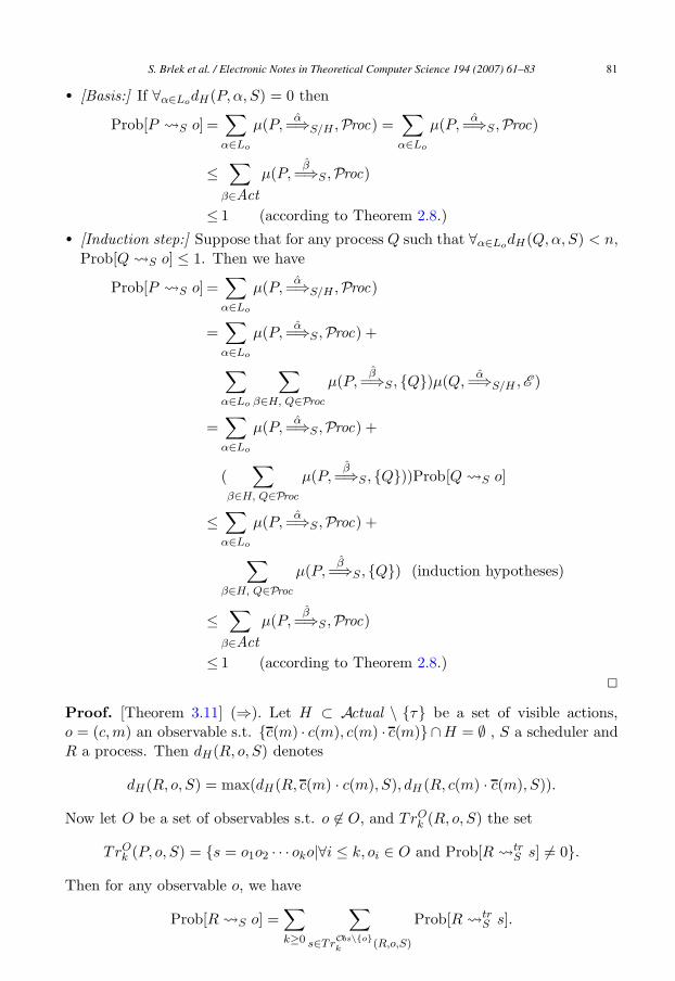
• [Basis:] If ∀α∈LodH(P,α, S) = 0 then

Prob[P �S o] =∑α∈Lo

μ(P,α

=⇒S/H ,Proc) =∑α∈Lo

μ(P,α

=⇒S ,Proc)

≤∑

β∈Act

μ(P,β

=⇒S ,Proc)

≤ 1 (according to Theorem 2.8.)

• [Induction step:] Suppose that for any process Q such that ∀α∈LodH(Q,α, S) < n,

Prob[Q �S o] ≤ 1. Then we have

Prob[P �S o] =∑α∈Lo

μ(P,α

=⇒S/H ,Proc)

=∑α∈Lo

μ(P,α

=⇒S ,Proc) +

∑α∈Lo

∑β∈H, Q∈Proc

μ(P,β

=⇒S , {Q})μ(Q,α

=⇒S/H ,E )

=∑α∈Lo

μ(P,α

=⇒S ,Proc) +

(∑

β∈H, Q∈Proc

μ(P,β

=⇒S , {Q}))Prob[Q �S o]

≤∑α∈Lo

μ(P,α

=⇒S ,Proc) +

∑β∈H, Q∈Proc

μ(P,β

=⇒S , {Q}) (induction hypotheses)

≤∑

β∈Act

μ(P,β

=⇒S ,Proc)

≤ 1 (according to Theorem 2.8.)

�

Proof. [Theorem 3.11] (⇒). Let H ⊂ Actual \ {τ} be a set of visible actions,

o = (c,m) an observable s.t. {c(m) · c(m), c(m) · c(m)} ∩H = ∅ , S a scheduler and

R a process. Then dH(R, o, S) denotes

dH(R, o, S) = max(dH(R, c(m) · c(m), S), dH (R, c(m) · c(m), S)).

Now let O be a set of observables s.t. o �∈ O, and TrOk (R, o, S) the set

TrOk (P, o, S) = {s = o1o2 · · · oko|∀i ≤ k, oi ∈ O and Prob[R �

trS s] �= 0}.

Then for any observable o, we have

Prob[R �S o] =∑k≥0

∑

s∈TrObs\{o}k (R,o,S)

Prob[R �trS s].

S. Brlek et al. / Electronic Notes in Theoretical Computer Science 194 (2007) 61–83 81

Let P and Q be two processes s.t. P �tr Q, o = (c,m) ∈ Obs , (Π, S) ∈ E ,

q ∈ Poly and

H = {α | ∃(c′,m′) ∈ Obs \ {o} and α ∈ {c′(m′) · c′(m′), c′(m′) · c′(m′)}}.

To prove the theorem, we proceed by induction on

max(dH(P |Π, o, S), dH (Q|Π, o, S)).

[Basis:] If dH(P |Π, o, S) = dH(Q|Π, o, S) = 0, then we have:

Prob[P |Π �S o] = μ(P |Π,α

=⇒S ,Proc) + μ(P |Π,β

=⇒S ,Proc)

where α = c(m) · c(m) and β = c(m) · c(m). Similarly

Prob[Q|Π �S o] = μ(Q|Π,α

=⇒S ,Proc) + μ(Q|Π,β

=⇒S,Proc).

P �tr Q ⇒

|μ(P |Π,α

=⇒S ,Proc) + μ(P |Π,β

=⇒S ,Proc)

−μ(Q|Π,α

=⇒S ,Proc) + μ(Q|Π,β

=⇒S ,Proc)| ≤1

q(N)

Hence

|Prob[P |Π �S o] − Prob[Q|Π �S o]| ≤1

q(N)

[Induction step:] assume that max(dH(P |Π, o, S), dH (Q|Π, o, S) = n, and ∀q∈Poly

we have

∑k<n

∑

s∈TrObs\{o}k (R,o,S)

|Prob[P |Π �trS s] − Prob[Q|Π �

trS s]| ≤

1

2q(N).

Now set Uk = TrHk (P |Π, o, S) ∪ TrH

k (Q|Π, o, S), then we have

|Prob[P |Π �S o]−Prob[Q|Π �S o]|

= |∑k≤n

∑s∈Uk

(Prob[P |Π �trS s] − Prob[Q|Π �

trS s])|

≤ |∑k<n

∑s∈Uk

Prob[P |Π �trS s] − Prob[Q|Π �

trS s]|

+∑s∈Un

|Prob[P |Π �trS s] − Prob[Q|Π �

trS s]|

By induction hypothesis we have

|∑k<n

∑s∈Uk

Prob[P |Π �trS s] − Prob[Q|Π �

trS s]| ≤

1

2q(N).

S. Brlek et al. / Electronic Notes in Theoretical Computer Science 194 (2007) 61–8382

Set rn = |TrHn (P |Π, o, S)| + |TrH

n (Q|Π, o, S)|. P �tr Q ⇒ ∀s ∈ Un

|Prob[P |Π �trS s] − Prob[Q|Π �

trS s]| ≤

1

rn · 2q(N),

then

∑s∈Un

|Prob[P |Π �trS s] − Prob[Q|Π �

trS s]| ≤

rn

rn · 2q(N)=

1

2q(N).

Hence we have

|Prob[P |Π �S o] − Prob[P |Π �S o]| ≤1

2q(N)+

1

2q(N)

≤1

q(N).

(⇐). Suppose now that P � Q but P ��tr Q. Then we will show that we

reach a contradiction. Indeed, if P ��tr Q, then there exists an attacker (Π, S), an

observable trace o1o2 · · · on and a polynomial q s.t.

∀N |Prob[P |Π �trS o1o2 · · · on] − Prob[Q|Π �

trS o1o2 · · · on]| >

1

q(N).

Let o′ = (c′,m) s.t. c′ is neither a channel of P or Q nor a channel of Π and

let (Π′, S′) be the attacker who behaves exactly like (Π, S) exept that anytime he

observes the trace o1o2 · · · on he makes the observable o′ with probability 1. Then

we have

|Prob[ P |Π′�

′S o′] − Prob[Q|Π′

�′S o′]|

= |Prob[P |Π �trS o1o2 · · · ono′] − Prob[Q|Π �

trS o1o2 · · · ono′]|

Hence P �� Q which contradicts our hypothesis. �

S. Brlek et al. / Electronic Notes in Theoretical Computer Science 194 (2007) 61–83 83