1

Tr ip scheduling on single track networks -the TUFF train scheduler

Per Kreuger , Mats Car lsson, Jan Olsson, Thomas Sjöland, Emil Åström

email: piak@sics.se

Swedish Institute of Computer Science (SICS)Box 1263, SE-164 29 Kista, Sweden

Abstract

A novel constraint model for scheduling train trips on a network of tracks used inboth directions is described. We argue that a generalization of a job-shop schedulingformulation can drastically decrease the problem size. Preliminary complexity andperformance results and a set of examples of schedules generated by our implementa-tion are presented.

1 Introduction

To schedule train trips on a network of tracks is an optimization problem that resembles butalso differs in certain ways from other typical scheduling tasks. The paper describes a con-straint model [VH 89] and solver for scheduling trains on a network of single tracks used inboth directions. This kind of problem can be modelled as a job-shop scheduling (JSS) prob-lem [CP 89, AC 91] regarding train trips as jobs to be scheduled on tracks regarded asresources. Each train trip traversing a track represents a task where the traversal time is takenas the duration of the task. Since the tracks can be used in both directions the JSS formula-tion requires each trip to demand exclusive use of the track as a resource for the duration ofthe track traversal. In order to achieve reasonable schedules with such a model it is necessaryto keep traversal times and hence individual tracks short. This results in very large schedul-ing problems (in terms of the number of tasks).

By generalizing this model to take into account two distinct durations for each task weare able to use a much coarser net without losing precision. Since train trips travelli ng inthe same direction no longer require exclusive use of the track resource for the duration ofthe traversal time the network can be used more eff iciently without increasing the granular-ity of the network representation.

The problem can be concisely stated as:

• Schedule a set of train trips over a fixed network of predetermined paths where trainstravel in both directions on single tracks connecting nodes where trains can meet andovertake

• Maintain reasonable bounds on waiting and total times

The rest of the paper is organized as follows: First comes an introductory note ill ustrating ageometric interpretation of our model. This is followed by a short description of the networkrepresentation used and how the problem specifications are built and maintained in the form

2

of a data structure (object representation) we call plans. Then we describe the constraintmodel used and formulate constraints stating soundness criteria of the generated schedules.This section is concluded with a discussion of the enumeration strategy used and some pos-sibil ities for improvement in this area.

We then briefly consider some complexity and performance issues and conclude thepaper with some notes on limitations in the model, some possible lines of future work andwith a set of examples.

2 A geometr ic intuition

The following two diagrams illustrate the difference between a job-shop scheduling formu-lation and our model. We use an adaptation of diagrams traditionally used to represent trainschedules. Time is on the axis and the height of each track represents the spatial distancebetween the end points of each track.

In the JSS formulation (fig. 1) there is only one duration associated with each start time.This duration, which we call traversal time, is ill ustrated as the width of each task rectan-gle. Rectangles on a single track must not overlap and track traversals belonging to a singletrip follows in sequence.

Another relevant duration is the headway, i.e. the (time) distance between any two trainsdeparting from some location in the same direction on single track.

In the second diagram (fig. 2) the width of each rhombus represents the headway whileits extension in the x-axis represents the traversal time. The angle of the rhombus repre-sents the speed of each individual traversal. In the example below we have chosen to giveslow trains a long headway and quick trains a short headway.

(Fig. 1)

(Fig. 2)

x

1:3

T 2

JSS formulation

T 4

T 1

T 3

1:1

1:4

1:22:3

2:2

2:43:1

3:2

3:4

3:3

4:1

4:3

4:2

4:4

2:1

T 2

Distinct headway and traversal time

T 4

T 1

T 3 1:3

2:1 3:44:1

4:2 5:3

5:4

6:3

1:46:4

2:2

1:1 3:1 4:46:12:4 5:1

2:3 1:23:2 4:35:2 6:2

3:3

3

It is easy to see that for comparable total times the number of trains that can be scheduledwith JSS on an identical network is significantly lower. It is possible to achieve a schedulesimilar to the second one using a network with a larger number of (shorter) tracks but thenthe size of the scheduling problem increases accordingly.

If job-shop scheduling can be seen as the problem of packing the rectangles of the regu-lar Gantt diagram under the precedence constraints imposed by the jobs, the single tracktrain scheduling problem can be seen as the corresponding rhombus packing problem.

3 Network representation

A rail road network is represented as three interrelated sets:

• Locations (nodes)

• Tracks (arcs)

• Predetermined paths

Each location is characterized by a unique name, geographical coordinates, a set of tracksadjoined to it and a set of paths passing through it while a track encodes the two locationsat its end points, a unique name, a length and a maximum speed at which trains may traverseit. Each path, on the other hand, is determined by a unique name and an ordered sequenceof directed track traversals.

4 Problem representation - plans

We use the notion plan to denote a data structure representing a scheduling problem in termsof a given network and a set of required train trips with limitations on departure and arrivaltimes at the start and end points of a given path.

Trips are determined by the path the train is required to traverse, the specification of con-straints on arrival and departure times at start and end points of the path, average speed forinvolved vehicles and a unique name.

The scheduling problem is extracted from the plan as a set of trips each consisting of aset of time slots representing the track traversals of the trip in the required schedule. Fur-thermore the set of slots associated with each track and path is extracted.

Each slot encodes a (unique) name, the name of a train trip traversing a track, the nameof the traversed track, the direction of the track traversal, headway and traversal times.

The scheduling problem can now be solved by imposing inequalities for all departureand arrival times associated with each trip, serializing the slots associated with each trackand searching for schedules consistent with these constraints.

In this process we can choose to constrain also the (accumulated) waiting and total timefor each trip and the total time required to execute the entire schedule. There is a trade-offbetween these two quali ty measures of the generated schedule such that plans with highdemands on (short) waiting times will , in general, have a longer total time and vice versa.See the examples of section 10.1 for an ill ustration of this phenomenon.

4

5 Constraint model

Slots represent traversals of tracks by trips at specific time intervals. We use a vector of finitedomain variables to represent departure times for such traversals and associate with eachslot a variable and not one but two constant durations:

• headway: (time) distance between any two trains departing from some location in thesame direction on single track

• traversal time: time during which no two trains in opposite direction may use a singletrack

This model is similar to those used for job-shop scheduling (see e.g. [CP 89, AC 91]) but dif-fers essentially in the use of two durations for each task. The model resembles JSS if foreach slot headway is identical to traversal time i.e. if no two trains can ever simultaneouslyuse the same track.

5.1 Constraints

There are two distinct sets of constraints used in the model. The first set is for maintainingthe precedence of the track traversals for each single trip. The only uncertainty here is howmuch slack (waiting time) to allow at each node, for each trip and for the complete schedule.

The second set of constraints is used to enforce a satisfiable serialization of all the slotsassociated with each track. To summarize:

1. For each trip all track traversals must follow in the sequence defined by its path and notoverlap

2. For each track

• Any two trains travell ing in the same direction must respect headway (even if speedsare different)

• Any two trains in opposite direction must not simultaneously use the same (single)track

We will now examine the formulation of these constraints in some detail .

5.1.1 Tr ip constraints

For all slots associated with a trip select uniquely:

• One finite domain variable to represent departure time

• One finite domain variable to represent waiting time (slack) at the location at the endof the traversal

and state:

• One sum constraint per slot to represent precedence between departure and arrivaltimes and upper bounds on waiting times

More formally, assume that we have for each trip unique finite domain variables represent-ing departure and arrival times, and , and a vector of slots

representing the tracks the trip traverses. Assume furthermore that this vector isDepTimei ArrTimei Tripi

Tripij

5

ordered by the path the trip traverses. Let the slots be represented as records using “ .” as afield access operation and use the fields , , and to represent the departure time, the waiting time at the end of the traversal, the traversal timeand (local) headway of the slot. The first two contain unique finite domain variables whilethe second two are fixed durations associated with the slot. The following equality betweenthe departure time of the first slot and that of the whole trip must hold:

then for each slot in the vector but the last the following equali ty must hold:

For the last slot this is replaced by:

and

The waiting times at each location can furthermore be limited either individually or by sumsover the waiting times associated with each trip. In addition we may state limits on the latestarrival time allowed in a particular schedule. These two parameters can, as we shall l ater see,be used to select schedules with different properties.

5.1.2 Track constraints

Define a disjointness constraint as:

which may be implemented e.g. by constructive disjunction.Then, for each track traversed by some trip:

1. For each pair of trips traversing a single track in the same direction a disjointness con-straint ensures that headway is respected at both departures and arrivals.

2. For each pair of trips traversing the track in opposite directions a disjointness constraintensures that trains will not colli de.

This second case corresponds to exclusive use of the track as resource and is equivalent tothe situation in job-shop scheduling. The first case however uses essentially the fact that weconsider two distinct durations for each slot.

Assume furthermore that we have for each track a set of slots denoted representing all trips traversing the track. Then for each pair of slots inthe set:

1. If the two trips traverse the track in the same direction the following (constraint) musthold

depTime waitTime travTime headway

Tripi1.depTime DepTimei=

Tripij

Tripij.depTime Tripij.travTime Tripij.waitTime+ + Tripi j 1+( ).depTime=

Tripin

Tripin.depTime Tripin.travTime+ ArrTimei= Tripin.waitTime 0=

Disjoint T1 D1 T2 D2, , ,( ) T1 D1+ T2≤( ) T2 D2+ T1≤( )∨⇔

Tracki TrackijTrackik Trackil( , )

Disjoint Trackik.depTime Distanceikl Trackil.depTime Distanceilk, , ,( )

6

where

Note that this formalization in itself does not guarantee that two trains running in thesame direction will not run into each other. This is the case only when the local head-ways (for each slot) are longer than the maximum traversal time variance.

2. If the two trips traverse the track in opposite directions instead the following (con-straint) must hold

Note the similarity with the standard job-shop scheduling formulation in the simple case ofavoiding colli sions (2). The choice between the two cases is completely determined by therelative direction of the traversals and does not in itself generate search.

The strength of the model is to a large extent determined by the propagation of the dis-junctions implicit in the disjointness constraints. Standard operational semantics of con-structive disjunction (see e.g. [BP 95]) seems to provide reasonable propagation.

There are more intricate issues involving search. We will briefly sketch some of them inthe following section.

5.2 The constraint solver

Since the model implicitly uses disjunctions in the disjointness constraints for the tracks, toenumerate the departure times generally involves search. We have investigated two distinctmethods to do this.

• The most straightforward approach is to enumerate the departure times themselvesin some order, rely on propagation to further restrict the domains of remaining depar-ture times and to detect failure in the case of an inconsistent instantiation.

• An alternative approach is to serialize all the slots for each track. The propagationbehaviour of constructive disjunction then ensures that enumeration of the departuretimes can be done without search if the minimum or maximum value of each domainis consistently chosen (See e.g. [BP 95]). This possibilit y and its implications is fur-ther discussed in section 8.1.

5.2.1 Enumeration of depar ture times

The performance figures given in section 7 below was achieved with an approach using thenumber of constraints associated with each variable as a variable ordering criterion andbisecting the domain of each departure time trying first the lower half of the domain for eachvariable.

Clearly such a strategy does not lend itself well to optimization. The search tree for thisformulation is simply too large. However given reasonable upper bounds on waiting timesit is a quick way to find good solutions. Unfortunately search explodes when the bounds

Distanceixymax Headwayix Headwayix Trackix.travTime Trackiy.travTime–+,( )

=

Disjoint Trackik.depTime Trackik.travTime Trackil.depTime Trackil.travTime, , ,( )

7

place us close to optimal total time which effectively excludes branch and bound search foroptimal solutions.

6 Some complexity results

For most realistic problems it is not entirely clear what is a good problem size measure. Thenumber of trips for a given net is a measure which comes naturally to mind but the numberof slots for problems sharing such a size varies irregularly with the particular paths selectedfor each problem, at least for small problems sizes (number of trips less than 100 on a net-work of about 45 nodes).

Even if we use the number of slots as a size measure, the complexity varies with theactual selection of paths in the problem. This phenomenon arises because the number ofconstraints grows quadratically with the number of slots associated with each single track.Some problems distribute their slots evenly over the tracks. These are relatively easy prob-lems. Diff icult problems have a few very “ tight” tracks with a large number of slots. Forsuch problems the number of constraints can grow very quickly.

The number of variables used to represent the problem are first of all 2 for each slot: Onefor the departure time and one for the waiting time. From a complexity point of view thesecond is redundant but in practice it is essential.

There is furthermore one arithmetic equality constraint stated for each slot. So far every-thing is linear. The real complexity comes from the serialization of the track traversals. Westate one disjointness constraint for each pair of trips traversing it. This operation amountsto finding each subset of size 2 of the slots associated with a track, i.e.

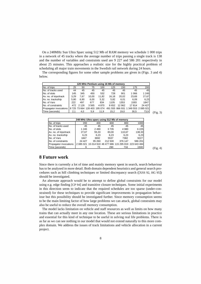
where the measure is the number of trips traversing a single track.For most realistic problems average and maximum will vary greatly from track to

track and from plan to plan. Some typical averages are listed in (Figs. 3 and 4) below.

7 Performance

Performance figures are rough and since the main limitation is memory the problem size wecan handle is not really large enough to do a more thorough empirical time complexity anal-ysis.

We currently schedule 200 trips traversing on the average 6 tracks each in a network con-sisting of 45 tracks where the average number of trips passing a single track is 28 and thenumber of variables and constraints used are 5541 and 73281 respectively. A first scheduleis found in about 74 seconds on a 120 Mhz Pentium PC with 40 MB of RAM memory. Thisis searching for a “good” but not necessarily optimal solution (in terms of total time to exe-cute the complete plan) where individual waiting times are bounded by a fixed (5%) frac-tion of the traversal time. Optimal solutions for smaller examples can be found by(manually) decreasing an upper bound for the total time but for larger examples (trips) search times tends to increase very fast close to an optimal solution.

N

2 N N 1–( )

2---------------------- O N

2( )= =

NN

> 60

8

On a 248MHz Sun Ultra Sparc using 512 Mb of RAM memory we schedule 1 000 tripsin a network of 45 tracks where the average number of trips passing a single track is 138and the number of variables and constraints used are 9 227 and 586 201 respectively inabout 25 minutes. This approaches a realistic size for the highly practical problem ofscheduling all major train movements in the Swedish rail network during 24 hours.

The corresponding figures for some other sample problems are given in (Figs. 3 and 4)below.

(Fig. 3)

(Fig. 4)

8 Future work

Since there is currently a lot of time and mainly memory spent in search, search behaviourhas to be analysed in more detail . Both domain dependent heuristics and general search pro-cedures such as hill climbing techniques or limited discrepancy search ([XSS 92, HG 95])should be investigated.

An alternate approach would be to attempt to define global constraints for our modelusing e.g. edge finding [CP 94] and transitive closure techniques. Some initial experimentsin this direction seem to indicate that the required schedules are too sparse (under-con-strained) for these techniques to provide significant improvements in propagation behav-iour but this possibility should be investigated further. Since memory consumption seemsto be the main limiting factor of how large problems we can attack, global constraints mayalso be useful to reduce the overall memory consumption.

The model lacks limitation on vehicle and staff resources as well as limits on how manytrains that can actually meet in any one location. These are serious limitations in practiceand essential for this kind of technique to be useful in solving real li fe problems. There isas far as we can see nothing in our model that would not extend naturally to this more com-plex domain. We address the issues of track limitations and vehicle allocation in a currentproject.

120 MHz Pentium using 16 Mb of memoryNo. of trips 25 50 75 100 125 150 175 200No. of tracks used 44 45 45 45 45 45 45 45No. of slots 145 345 450 532 728 901 1 066 1 245Av. no. of trips/track 3,29 7,67 10,00 11,82 16,18 20,02 23,69 27,67Av. no. tracks/trip 5,80 6,90 6,00 5,32 5,82 6,01 6,09 6,23No. of Vars 222 497 677 834 1105 1353 1593 1847No. of constraints 472 2 126 3 565 4 870 8 652 12 962 17 814 24 427Propagator invocations 8 725 73 664 128 403 195 074 491 555 866 931 1 349 553 2 085 021Time (seconds) 2,1 4,0 5,9 11,9 15,2 19,0 30,5 73,9

248 MHz Ultra sparc using 512 Mb of memoryNo. of trips 200 400 600 800 1000No. of tracks used 45 45 45 45 45No. of slots 1 245 2 490 3 735 4 980 6 225Av. no. of trips/track 27,67 55,33 83,00 110,67 138,33Av. no. tracks/trip 6,23 6,23 6,23 6,23 6,23No. of Vars 1847 3692 5537 7382 9227No. of constraints 24 427 95 260 212 500 376 147 586 201Propagator invocations 2 085 021 15 014 919 48 477 686 115 295 819 223 643 484Time (seconds) 9 73 290 716 1500

9

In practice it will probably also be both possible and necessary to subdivide the completeproblem into several smaller and relatively independent sub-problems. For larger realisticproblems such as producing schematic schedules several months in advance problem sub-division is most likely the only possible approach. The standard way to do this is to subdi-vide the problem into that of producing several weekly and daily schedules and to dodetailed scheduling for separate geographic regions given non-local constraints on e.g.interregional trains. This aspect is also addressed in the current project.

8.1 Enumeration of boolean var iables representing serialization choices

We have been experimenting with serializing the slots for each track before actually assign-ing values to the departure times but have so far not been able to reproduce the performanceresults given with the naive strategy above. It appears that enumerating departure times givesbetter propagation thus eliminating most of the search while a bad serialization choice earlyin the enumeration process can potentially generate a huge amount of search much later.

We believe however that this approach wil l eventually prove to be superior. First thesearch tree in this formulation identifies all solutions that do not result in a reordering ofthe slots within a given track. This means that it wil l be more realistic to search for optimalor close to optimal solutions, possibly using the naive approach to determine reasonableupper bounds.

Second it is possible with such an approach to formulate very intricate search strategies.It may e.g. be a good idea to first serialize the tracks with the largest number of slots orwith the largest number of constraints summed over all its slots. Such tracks would repre-sent tight resources in the network.

It could also be a good idea to choose first to serialize long tracks or to use the fact thatthe upper bound on total time is to a large extent dependent on a few relatively long trips, atleast for the kind of problem sizes considered so far.

To formulate a good strategy using such ideas is of course not trivial and presently repre-sents future work. It may also turn out that generalizing existing methods to implementglobal constraints for job-shop scheduling problems e.g. edge finding (see e.g. [BP 95])and/or transitive closure is feasible. This would represent a complementary approach torefining the present results.

Choosing to represent potential schedules by a boolean vector also allows for more flexi-ble rescheduling and incremental updates of existing schedules. Investigations of theseaspects of constraint programming is currently under way within our group.

9 Conclusions

We have described a novel constraint model for train scheduling and evaluated a correspond-ing solver on a number of realisticall y sized problems. With a relatively straightforwardsolver we have been able to attack problems approaching those appearing in actual practice.It is notable also that even though the simple solver we used in the performance tests doesnot lend itself well to optimization, the schedules found are in general quite close to manu-ally found optima.

10

Our modelli ng approach seem therefore to represent a major improvement of more tradi-tional alternatives.

10 Sample schedules

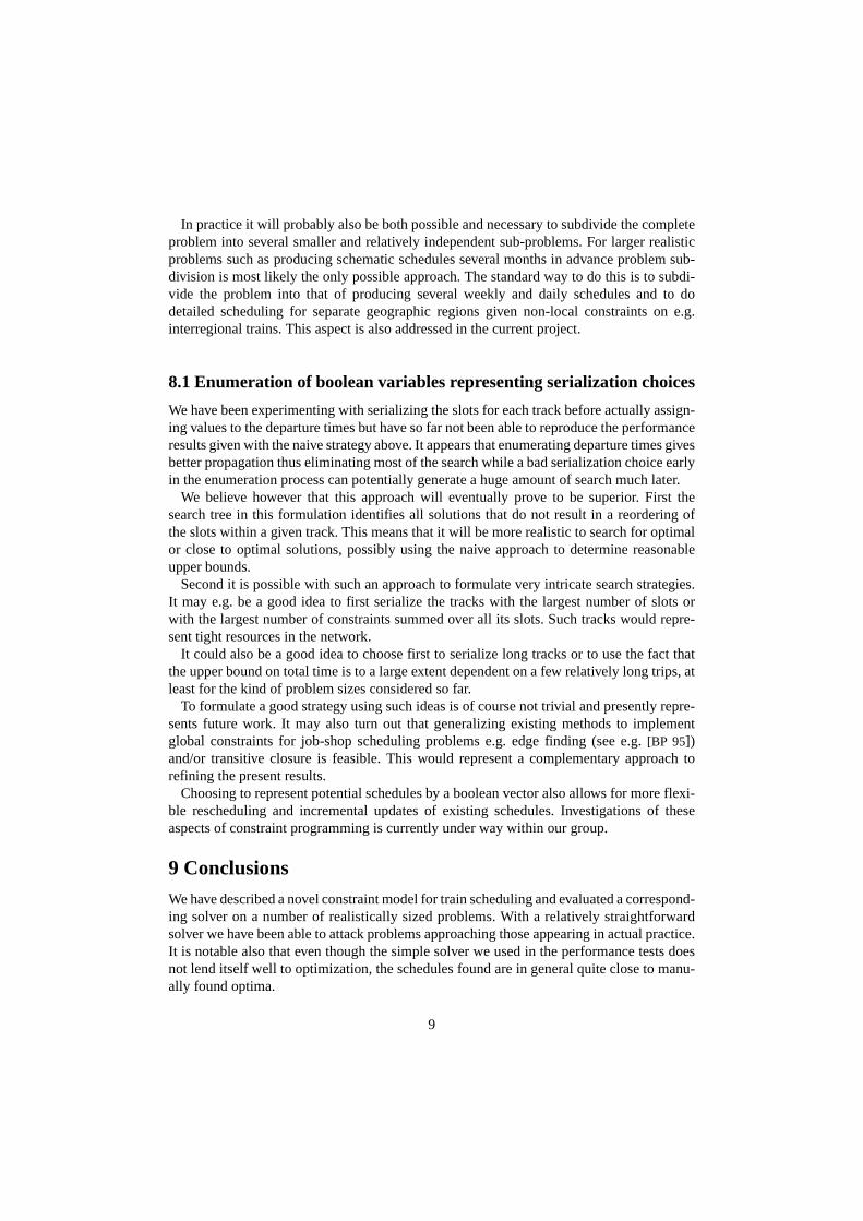
The following diagrams illustrate some sample schedules generated by our implementation.The implementation was done completely in the Oz programming language [Sm 95, ST 95]using the embedded Tcl/Tk interface for the GUI parts. The diagrams encode time on the axis and spatial distance between locations on a given path on the axis. The width of therhombi representing the trips encode the variance of traversal time for each track traversal.The angle of the rhombi sides encodes the speed of the train during the traversal with angleslarger than encoding trips moving in opposite direction.

10.1 Trade-off between total time and waiting time

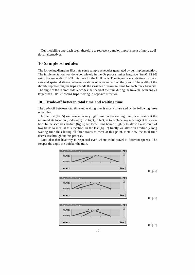
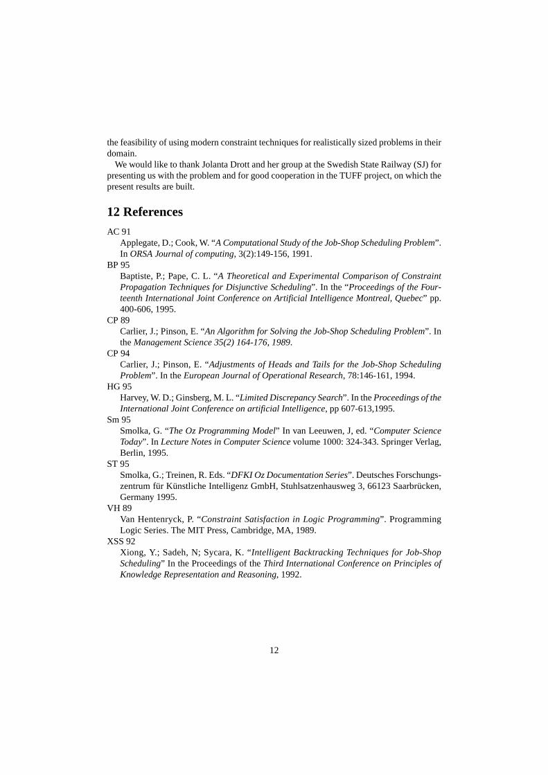
The trade-off between total time and waiting time is nicely il lustrated by the following threeschedules.

In the first (fig. 5) we have set a very tight limit on the waiting time for all trains at theintermediate location (Södertälje). So tight, in fact, as to exclude any meetings at this loca-tion. In the second schedule (fig. 6) we loosen this bound slightly to allow a maximum oftwo trains to meet at this location. In the last (fig. 7) finally we allow an arbitrarily longwaiting time thus letting all three trains to meet at this point. Note how the total timedecreases throughout this process.

Note also that headway is respected even where trains travel at different speeds. Thesteeper the angle the quicker the train.

(Fig. 5)

(Fig. 6)

(Fig. 7)

xy

90°

11

10.2 Some larger schedules

The following examples illustrate some larger schedules and how much bounds on the wait-ing times influences the sparseness of the schedules. The following diagrams represent iden-tical fragments (all traversals of the tracks of one particular path) of 2 different 60 tripschedules. The first (fig. 8) with low tolerance on waiting times, the second (fig. 9) with hightolerance on waiting times. Note also how the total time is decreased with about 25% bybounding waiting times to allow approximately three trips to meet at each location.

(Fig. 8)

(Fig. 9)

11 Acknowledgements

The work reported in this paper is one of the results of a pilot study done in cooperation withthe Swedish State Railway (SJ). The motivation behind this cooperation has been to evaluate

12

the feasibilit y of using modern constraint techniques for realistically sized problems in theirdomain.

We would like to thank Jolanta Drott and her group at the Swedish State Railway (SJ) forpresenting us with the problem and for good cooperation in the TUFF project, on which thepresent results are built .

12 References

AC 91Applegate, D.; Cook, W. “A Computational Study of the Job-Shop Scheduling Problem” .In ORSA Journal of computing, 3(2):149-156, 1991.

BP 95Baptiste, P.; Pape, C. L. “A Theoretical and Experimental Comparison of ConstraintPropagation Techniques for Disjunctive Scheduling” . In the “Proceedings of the Four-teenth International Joint Conference on Artificial Intelligence Montreal, Quebec” pp.400-606, 1995.

CP 89Carlier, J.; Pinson, E. “An Algorithm for Solving the Job-Shop Scheduling Problem” . Inthe Management Science 35(2) 164-176, 1989.

CP 94Carlier, J.; Pinson, E. “Adjustments of Heads and Tails for the Job-Shop SchedulingProblem” . In the European Journal of Operational Research, 78:146-161, 1994.

HG 95Harvey, W. D.; Ginsberg, M. L. “Limited Discrepancy Search” . In the Proceedings of theInternational Joint Conference on artificial Intelligence, pp 607-613,1995.

Sm 95Smolka, G. “The Oz Programming Model” In van Leeuwen, J, ed. “Computer ScienceToday” . In Lecture Notes in Computer Science volume 1000: 324-343. Springer Verlag,Berlin, 1995.

ST 95Smolka, G.; Treinen, R. Eds. “DFKI Oz Documentation Series” . Deutsches Forschungs-zentrum für Künstliche Intelli genz GmbH, Stuhlsatzenhausweg 3, 66123 Saarbrücken,Germany 1995.

VH 89Van Hentenryck, P. “Constraint Satisfaction in Logic Programming” . ProgrammingLogic Series. The MIT Press, Cambridge, MA, 1989.

XSS 92Xiong, Y.; Sadeh, N; Sycara, K. “ Intelligent Backtracking Techniques for Job-ShopScheduling” In the Proceedings of the Third International Conference on Principles ofKnowledge Representation and Reasoning, 1992.