Solar Energy Vol. 70, No. 1, pp. 13–22, 20012001 Elsevier Science Ltd

Pergamon PII: S0038 – 092X( 00 )00121 – 3 All rights reserved. Printed in Great Britain0038-092X/01/$ - see front matter

www.elsevier.com/ locate / solener

A HYBRID MODEL FOR ESTIMATING GLOBAL SOLAR RADIATION

†K. YANG , G. W. HUANG and N. TAMAIRiver Laboratory, Department of Civil Engineering, University of Tokyo, Bunkyo-ku, Tokyo 113-8656,

Japan

Received 15 December 1999; revised version accepted 31 July 2000

Communicated by RICHARD PEREZ

˚ ¨Abstract—In view of the site-dependence of Angstrom correlation, this study developed a hybrid model to˚ ¨estimate global radiation H. Unlike Angstrom correlation H 5 (a 1 bS /S )H , this model suggested that0 0

H 5 (a 1 b S /S )H 1 (c 1 d S /S )H , H and H are effective beam radiation and effective diffuse radiation,0 b 0 d b d

which imply latitude, elevation and seasonal effect on radiation. H and H are calculated by an arithmeticb d

model derived from spectral model. The hybrid model was designed for estimating monthly mean daily globalradiation with hourly-recorded bright sunshine time, and its applicability was verified at observatories in Japan. 2001 Elsevier Science Ltd. All rights reserved.

1. INTRODUCTION of S /S in Eq. (1). Gopinathan (1988) proposed a0

formula which relates latitude, elevation and S /S0Solar radiation received at the surface is ofto a and b. Yeboah-Amankwah and Agyeman

primary importance for the purpose of building(1990) believed that a and b are time-dependent

solar energy devices, estimating crop productivity, ˚ ¨and so developed a differential Angstrom modeletc. However, direct measuring is not available in

with a set of coefficients which vary with time.many cases, so numerical technique becomes an

Ninomiya (1994) considered the effect of snoweffective alternative to estimate global radiation

and rainfall of rainy days. Sahin and Sen (1998)through observed meteorological data.

proposed a method to dynamically estimate the˚ ¨The Angstrom (1924) correlation has served ascoefficients a and b. However, their work doesn’t

a basic approach to estimate global radiation for aconsider the radiation damping processes when

long time. Prescott (1940) has put the correlationsolar rays pass through the atmosphere. Some

in a convenient form asresearchers (Leckner, 1978; Bird, 1984) employeda damping spectrum to calculate global solarH 5 (a 1 bS /S )H (1)0 0radiation in clear sky. Their models consider

22 22where H (Jm ) and H (Jm ) are solar radiation physical processes in detail, so the effects of0

on a horizontal surface at ground level and at latitude, elevation and other factors are taken intoextraterrestrial level, respectively. S /S is the time account automatically. However, damping spec-0

fraction of bright sunshine, a and b are constants. trums are very irregular and hence a numerical˚ ¨The Angstrom formula only involves S /S and integration is indispensable, which is an onerous0

thus is quite convenient for application. Unfor- task. Furthermore, the uncertainties associatedtunately, it does not consider the effect of latitude with cloudiness limit the application of spectraland elevation, so a and b are site-based co- models.efficients. For instance, a 5 0.1 | 0.3, b 5 0.4 | 0.7 Therefore, this study attempts to develop ain China (Xu, 1993). Up to now, there are model that can consider the physical processes but

˚ ¨some attempts to explore more accurately a and b still maintain the simplicity of the Angstromor consider other factors such as elevation and correlation. In Section 2, a model form is pro-latitude. Iqbal (1979) appended a quadratic term posed to incorporate effective beam radiation and

diffuse radiation with global radiation. Then theLeckner spectral model is simplified to calculate

† effective beam radiation and diffuse radiation inAuthor to whom correspondence should be addressed. Tel.:Section 3. The model is calibrated in Section 4181-3-5841-6108; fax: 181-3-5841-6130; e-mail:

yangk@hydra.t.u-tokyo.ac.jp and its verification is carried out in Section 5.

13

14 K. Yang et al.

2. NEW FORM OF SOLAR RADIATION the solar irradiance spectrum at extraterrestrialMODEL level, l and l are the lower and highermin max

wavelength limits of solar spectrum, respectivelyWhen solar rays pass through the atmosphere,

(Thekaekara, 1973). h(rad) is the altitude angle ofthere are five types of radiation-damping pro-

the sun, t(s) is the time.cesses, viz. Rayleigh scattering, aerosol extinc-

Effective beam radiation H and diffuse radia-btion, ozone absorption, water vapor absorptiontion H mainly vary with the position of the sun.dand permanent gas absorption, which are repre-Fig. 1 is an example to show its temporal

sented by transmittance functions t (l), t (l),oz w variation. The site is Tokyo and the date is Jul. 1,t (l), t (l), t (l), respectively. l(m) representsg r a 1996. The calculation follows the Leckner (1978)wave-length. In order to consider the effect of all

model (see Section 3). The horizontal axis repre-transmittance functions, we define the beam trans-

sents the daytime and the vertical H , H and their] ] b dmittances t and diffuse transmittance t asb d ratio H /H . During sunrise and sunset, thed b

diffuse radiation is higher than the beam radiationlmax

due to intense Rayleigh scattering and aerosol21]t ; I E I (l)t (l)t (l)t (l)t (l)t (l) dl,b 0 0i oz w g r a extinction. However, the former is much lowerlmin than the latter at noon. Therefore, the ratio H /Hd b

is not a constant. Actually, it depends on location,(2a)date and time, etc.

lmax In a cloudy sky, a part of H may directly passb21] through the cloud layer and arrive on the ground ast ; I E I (l)t (l)t (l)t (l)d 0 0i oz w g

beamradiation,whichisassumedas(a 1b S /S )H ,1 1 0 blmin

analogous to Eq. (1); also, a part of H may beb3 [1 2 t (l)t (l)] dl. (2b)r a diffused by the cloud layer but finally arrive onthe ground as diffuse radiation, which is assumed

22And define effective beam radiation H (J m )b as the (a 1 b S /S )H . Similarly, we assume2 2 0 b22and diffuse radiation H (J m ) at ground leveld the diffuse radiation from H is (c 1 dS /S )Hd 0 das after the reflection and scattering at the cloud

layer. Therefore, the global radiation H is the sum] of the three parts, which has the form as below,H ; I E t sin h dt, (3a)b 0 b

H 5 (a 1 b S /S )H 1 (c 1 d S /S )H (4)0 b 0 d]H ; I E t sin h dt, (3b)d 0 d

where a, b, c and d are coefficients. a and a are1 2l 22 21max merged as a, b and b are merged as b, so thewhere I 5 e I (l) dl. I (wm mm ) is 1 20 l 0i 0imin

Fig. 1. Temporal variation of effective beam radiation H , diffuse radiation H , and the ratio H /H . Date: Jul. 1, 1996. Place:b d d b

Tokyo (1398469E, 358419N).

A hybrid model for estimating global solar radiation 15

term (a 1 b S /S )H includes both beam and unavailable, its value is estimated through0 b

diffuse radiation. Eq. (4) is an analogue tol 5 0.44 2 0.16˚ ¨Angstrom correlation Eq. (1), but H and H areb d 2 2 1 / 23 h[(f 2 80) /60] 1 [(d 2 120) /(263 2 f)] j ,calculated from spectral model as follows, so it is

a hybrid model. with

J if J , 300d dd 5H] ] J 2 366 if J . 3003. SIMPLIFIED MODEL FOR t AND t d dB D

To estimate global radiation, H and H have to which is a roughly fitting formula based on Fig.b d

be calculated at first. Since, altitude angle h in the 9.12 of Xu (1993), J is the Julian day. T (8C)d dew2Eqs. (3) can be easily calculated, the main is dew point, and w (g /cm ) is precipitable water

21difficulty lies in the integration of beam transmitt- w 5 0.493(T 1 273.15) exp[26.23 2 5416dew21 21] ]ances t and diffuse transmittance t through Eqs. (T 1 273.15) ]. k , k , k (cm ) are absorp-b d dew oz w g

(2). As mentioned above, this costly integration is tion coefficients of ozone, water vapor and perma-one weakness of the spectral model. The purpose nent gases, respectively. P (mb) is local pressure,

3of this section is to explore a simple method to and P 5 1.013 3 10 mb.0] ˚replace numerical integration for calculating t ¨Since Angstrom turbidity, thickness of ozoneb

]and t . layer and precipitable water vary with season,d

As shown in Leckner (1978) spectral model, latitude and/or elevation, the transmittance func-the five transmittance functions in Eqs. (2) can be tions have considered their effect on solar radia-expressed as: tion. In order to simplify the calculation of Eqs.

(2), we derive each energy-weighted averaget (l) 5 exph 2 lmk (l)j, (5a)oz oz transmittance function as follows.

For the transmittance function due to ozoneabsorption, it is defined ast (l) 5 exph[20.2385k (l)mw]w w

0.45 lmax/ [1 1 20.07k (l)mw] j, (5b)w

21]t ; I E I (l)t (l) dloz 0 0i oz

t (l) 5 exph lg min

l0.45 max2 1.41k (l)m / [1 1 118.3k (l)m] j,g g21

5 I E I (l) exp(2lmk (l)) dl (6)0 0i oz(5c)lmin

24.08 ]t (l) 5 exph 2 0.008735ml P/P j, (5d) Evidently, t is a function of ml rather thanr 0 oz

wavelength l. With the absorption coefficients21.3 k (l) provided by Leckner (1978), we can obtainozt (l) 5 exph 2 b ml j, (5e)a t

the transmittance due to ozone absorption throughnumerically integrating Eq. (6). As shown in Fig.where Air mass m 5 (1 2 0.0001z ) / [sinh 1s

21.253 2, the dots are integrated values. Fitting the0.15(57.296h 1 3.885) ]; z (m) is grounds˚ discrete data by least square method, we can¨level. b is Angstrom turbidity. If b is unavail-t t

obtain the following approximate relation.able, the following formula is adopted to estimate]its value: ]t 5 exp(2lmk ), (7a)oz oz

]b 5b 1 Db ,t t t Similar processing is applied to other transmitt-

ance functions. The final result is]b 5 (0.025 1 0.1 cos f) exp(20.7z /1000), ] ]t s t 5 exp(2c ) (7b)w w

] ]Db 5 6(0.02 | 0.06).t t 5 exp(2c ) (7c)g g

] ]24.08b is the annual mean values of turbidity, follow- ]t t 5 exp(20.008735ml P/P ) (7d)r r 0˚ ¨ing Fig. 3 of Angstrom (1961). Db is thet

]21.3seasonal deviation from the mean values, i.e. low ]t 5 exp(2b ml ) (7e)a t avalues in winter, high values in summer.l (cm) is the thickness of ozone layer. If l is where

16 K. Yang et al.

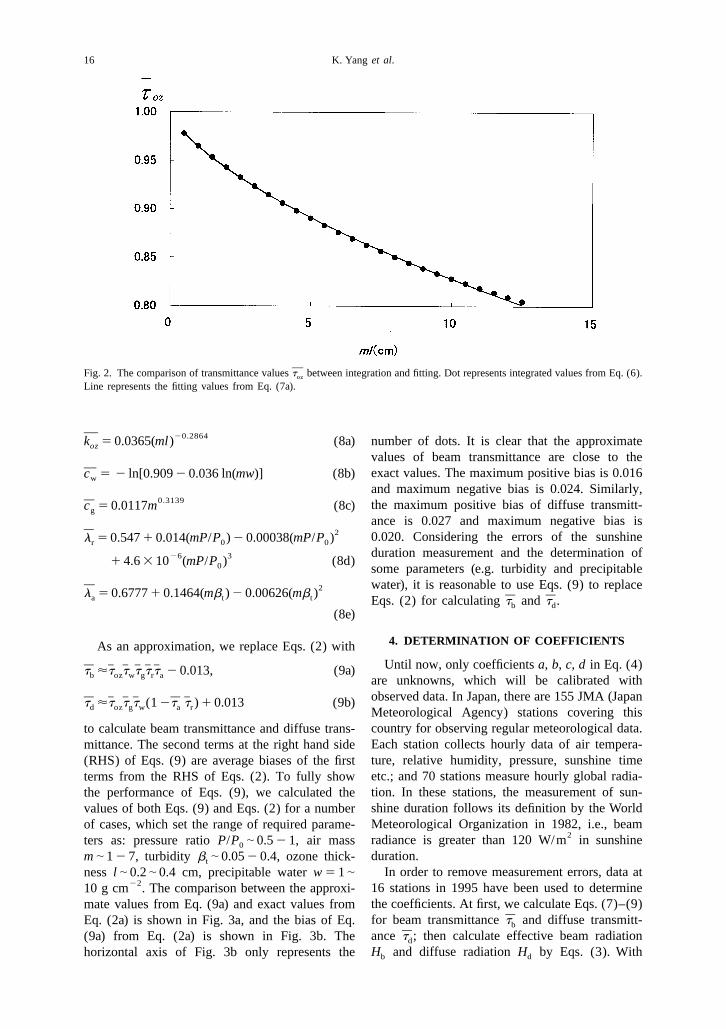
]Fig. 2. The comparison of transmittance values t between integration and fitting. Dot represents integrated values from Eq. (6).oz

Line represents the fitting values from Eq. (7a).

] 20.2864k 5 0.0365(ml) (8a) number of dots. It is clear that the approximateoz

values of beam transmittance are close to the] exact values. The maximum positive bias is 0.016c 5 2 ln[0.909 2 0.036 ln(mw)] (8b)w

and maximum negative bias is 0.024. Similarly,0.3139] the maximum positive bias of diffuse transmitt-c 5 0.0117m (8c)g

ance is 0.027 and maximum negative bias is] 2 0.020. Considering the errors of the sunshinel 5 0.547 1 0.014(mP/P ) 2 0.00038(mP/P )r 0 0

duration measurement and the determination of26 31 4.6 3 10 (mP/P ) (8d)0 some parameters (e.g. turbidity and precipitable

water), it is reasonable to use Eqs. (9) to replace] 2l 5 0.6777 1 0.1464(mb ) 2 0.00626(mb ) ] ]a t t Eqs. (2) for calculating t and t .b d

(8e)

4. DETERMINATION OF COEFFICIENTSAs an approximation, we replace Eqs. (2) withUntil now, only coefficients a, b, c, d in Eq. (4)] ] ] ] ] ]t ¯t t t t t 2 0.013, (9a)b oz w g r a are unknowns, which will be calibrated with

observed data. In Japan, there are 155 JMA (Japan] ] ] ] ] ]t ¯t t t (1 2t t ) 1 0.013 (9b)d oz g w a r Meteorological Agency) stations covering thiscountry for observing regular meteorological data.to calculate beam transmittance and diffuse trans-Each station collects hourly data of air tempera-mittance. The second terms at the right hand sideture, relative humidity, pressure, sunshine time(RHS) of Eqs. (9) are average biases of the firstetc.; and 70 stations measure hourly global radia-terms from the RHS of Eqs. (2). To fully showtion. In these stations, the measurement of sun-the performance of Eqs. (9), we calculated theshine duration follows its definition by the Worldvalues of both Eqs. (9) and Eqs. (2) for a numberMeteorological Organization in 1982, i.e., beamof cases, which set the range of required parame-

2radiance is greater than 120 W/m in sunshineters as: pressure ratio P/P | 0.5 2 1, air mass0

duration.m | 1 2 7, turbidity b | 0.05 2 0.4, ozone thick-t

In order to remove measurement errors, data atness l | 0.2 | 0.4 cm, precipitable water w 5 1 |22 16 stations in 1995 have been used to determine10 g cm . The comparison between the approxi-

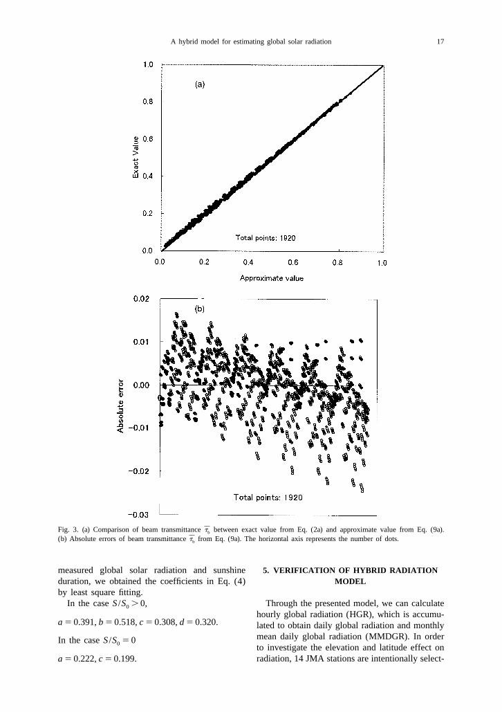
the coefficients. At first, we calculate Eqs. (7)–(9)mate values from Eq. (9a) and exact values from]for beam transmittance t and diffuse transmitt-Eq. (2a) is shown in Fig. 3a, and the bias of Eq. b

]ance t ; then calculate effective beam radiation(9a) from Eq. (2a) is shown in Fig. 3b. The d

H and diffuse radiation H by Eqs. (3). Withhorizontal axis of Fig. 3b only represents the b d

A hybrid model for estimating global solar radiation 17

]Fig. 3. (a) Comparison of beam transmittance t between exact value from Eq. (2a) and approximate value from Eq. (9a).b](b) Absolute errors of beam transmittance t from Eq. (9a). The horizontal axis represents the number of dots.b

measured global solar radiation and sunshine 5. VERIFICATION OF HYBRID RADIATIONduration, we obtained the coefficients in Eq. (4) MODELby least square fitting.

In the case S /S . 0, Through the presented model, we can calculate0

hourly global radiation (HGR), which is accumu-a 5 0.391, b 5 0.518, c 5 0.308, d 5 0.320. lated to obtain daily global radiation and monthly

mean daily global radiation (MMDGR). In orderIn the case S /S 5 00 to investigate the elevation and latitude effect onradiation, 14 JMA stations are intentionally select-a 5 0.222, c 5 0.199.

18 K. Yang et al.

˚ ¨Table 2. Coefficients of Angstrom correlation at 14 JMAed so that they include: the southernmost, thestations for 1995 (in case S /S . 0)0northernmost, the highest, the biggest city andStation a b a 1 bother stations distributing from south to north.

No.The geometrical parameters at these stations are

1 0.283 0.367 0.650shown in Table 1. So these stations with 7 0.272 0.374 0.646

8 0.315 0.410 0.725geometrical features are believed to represent all13 0.348 0.386 0.734stations in Japan.

˚ ¨Firstly, the applicability of Angstrom correla-tion in Japan is investigated. The coefficients a

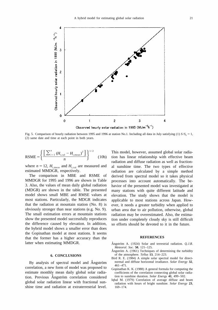
and b of Eq. (1) for four typical locations are (not shown). The analysis shows the causes of theregressed and shown in Table 2 for 1995. It is greater errors are different at the stations.obvious that: (1) a and b at southern station (No. 1) (1) At No. 1, the radiation may be under-are less than at northern station (No. 13) since measured due to system error in 1996. Fig. 5turbidity decreases with respect of increase of shows the measurement difference at this stationlatitude; (2) a and b at urbanized area (No. 7) are during July 1995 and 1996. Each point in thisless than at mountain (No. 8) due to lower figure satisfies (a) measurement under very clearturbidity and less air mass at mountain areas. If sky (S /S 5 1), and (b) same date and time except0

coefficients a and b from mountainous station that the horizontal axis represents the measured(No. 8) are applied to urbanized area (No. 7), the values in 1995 and the vertical one represents the˚ ¨Angstrom correlation will overestimate global measured values in 1996. This figure clearlyradiation more than 10%. Therefore, a and b are shows that the radiation in 1996 may be under-site-dependent in Japan. measured if the measurement in 1995 is correct,

Secondly, the estimation to MMDGR by the which leads to the greater deviation of estimationhybrid model is compared with observations at all from measurement.14 stations. Figs. 4a and b show the estimated and (2) The greater error at station No. 7 (Tokyo)observed MMDGR for 1995 and 1996, respective- may be caused by the larger turbidity in urbanly. The horizontal axis represents the observed areas due to air pollution. The radiation seems tovalues and the vertical axis represents the esti- be overestimated since the turbidity given in thismated values. Apparently, the estimation of model is an average value on longitude, which isMMDGR at most stations is quite close to the lower than that in urban areas.observation for both 1995 and 1996, which indi- (3) At No. 13–14, the error is mainly causedcates that the performance of the presented model owing to estimation difficulties under completelydoesn’t have obvious dependence on elevation, cloudy sky (S /S 5 0). Radiation in cloudy con-0

latitude or seasons. In other word, this model can ditions is very variable, so estimations error isaccount for the effect of elevation, latitude or usually larger than under clear conditions. Sinceseasons. However, some obvious errors are still stations No. 13–14 locate in northernmost Japan,found at station No. 7 and No. 13 for 1995, and the duration of completely cloudy sky (S /S 5 0)0

No. 1, No. 7, and No. 13–14 for 1996. It was is longer than that of sunshine and partial cloud-found that the errors at these stations are also covered sky (S /S . 0). Computation shows that0

greater than that at other stations even though the overall cloud duration contributes to about˚ ¨site-dependent Angstrom-type model is applied 1/4 of the total radiation, but to about half of the

Table 1. Geometrical parameters at 14 JMA stations

No. Station Longtitude (E) Latitude (N) Elevation (m)

1 Minamitorishima 1538589 248189 8.32 Naha 1278419 268129 28.03 Naze 1298309 288239 2.84 Kakoshima 1308339 318349 4.25 Fukuoka 1308239 338349 2.56 Kofu 1388339 358409 272.87 Tokyo 1398469 358419 5.38 Matsumoto 1378589 368159 610.09 Niigata 1398039 378559 1.9

10 Akita 1408069 398439 6.311 Hakodate 1408459 418499 35.012 Sapporo 1418209 438039 17.213 Kitamiesashi 1428359 448569 6.714 Wakkanai 1418419 458259 2.8

A hybrid model for estimating global solar radiation 19

Fig. 4. (a) Comparison of MMDGR between observation and estimation with hybrid model at 14 stations in Japan for 1995. (b)Comparison of MMDGR between observation and estimation with hybrid model at 14 stations in Japan for 1996.

errors. Therefore, the cloudy weather condition is 14 stations on both southern and northern hemi-one main contributor to the greater errors. sphere by Gopinathan. The mean bias error

Finally, the errors of MMDGR estimation are (MBE) and root mean square error (RMSE) arecompared between the hybrid model and the chosen to show the errors, which are defined asGopinathan (1988) model. The latter was de-

nveloped to estimate MMDGR with consideration F GO (H 2 H )i51 i,cal i,meas]]]]]]]of latitude and elevation, and has been verified at MBE 5 (10a)n

20K

.Yang

etal.

Table 3. Mean daily global radiation (MDGR) and errors of monthly mean daily global radiation predicted by hybrid model (HM) and Gopinathan model (GM)

Station No. 1 2 3 4 5 6 7 8 9 10 11 12 13 14

1 MDGR 17.89 13.64 12.08 14.22 13.73 14.30 12.16 14.80 11.70 11.21 11.81 11.51 11.26 12.8029 (MJ/m )

9 MBE HM 0.424 20.262 0.004 20.096 20.052 0.332 0.952 20.229 20.209 20.203 20.111 20.435 20.894 20.24325 (MJ/m ) GM 2.286 1.162 0.606 1.395 1.287 1.282 1.971 0.090 0.277 20.171 0.516 20.193 21.119 20.144

RSME HM 0.684 0.463 0.411 0.416 0.374 0.475 1.209 0.323 0.426 0.430 0.474 0.549 0.920 0.7732(MJ/m ) GM 2.371 1.277 0.737 1.494 1.413 1.433 2.153 0.660 0.874 0.589 0.818 0.535 1.136 0.852

1 MDGR 16.33 14.41 12.27 14.19 13.18 14.25 12.55 15.12 12.90 11.70 11.62 11.62 10.63 10.8229 (MJ/m )

9 MBE HM 1.180 20.495 0.007 20.220 20.027 20.495 0.732 20.266 20.326 20.080 20.158 20.512 20.731 21.02326 (MJ/m ) GM 3.172 1.155 0.977 1.198 1.241 1.255 1.914 20.042 0.430 0.279 0.363 20.314 21.030 21.541

RSME HM 1.406 0.631 0.446 0.358 0.315 0.565 0.823 0.348 0.542 0.467 0.460 0.689 0.920 1.2172(MJ/m ) GM 3.297 1.237 1.057 1.249 1.384 1.325 2.002 0.575 0.808 1.144 1.064 0.774 1.625 1.840

A hybrid model for estimating global solar radiation 21

Fig. 5. Comparison of hourly radiation between 1995 and 1996 at station No.1. Including all data in July satisfying (1) S /S 5 1,0

(2) same date and time at each point in both years.

n 1 / 22 This model, however, assumed global solar radia-F GO (H 2 H )i51 i,cal i,measH J]]]]]]]]RSME 5 (10b) tion has linear relationship with effective beamnradiation and diffuse radiation as well as fraction-

where n 5 12, H and H are measured and al sunshine time. The two types of effectivei,meas i,cal

estimated MMDGR, respectively. radiation are calculated by a simple methodThe comparison in MBE and RSME of derived from spectral model so it takes physical

MMDGR for 1995 and 1996 are shown in Table processes into account automatically. The be-3. Also, the values of mean daily global radiation havior of the presented model was investigated at(MDGR) are shown in the table. The presented many stations with quite different latitude andmodel shows small MBE and RMSE values at elevation. The study shows that the model ismost stations. Particularly, the MDGR indicates applicable to most stations across Japan. How-that the radiation at mountain station (No. 8) is ever, it needs a greater turbidity when applied toobviously stronger than near stations (e.g. No. 9). urban area due to air pollution, otherwise, globalThe small estimation errors at mountain stations radiation may be overestimated. Also, the estima-show the presented model successfully reproduces tion under completely cloudy sky is still difficultthe difference caused by elevation. In addition, so efforts should be devoted to it in the future.the hybrid model shows a smaller error than doesthe Gopinathan model at most stations. It seems

REFERENCESthat the former has a higher accuracy than the˚latter when estimating MMDGR. ¨Angstrom A. (1924) Solar and terrestrial radiation. Q.J.R.

Meteorol. Soc. 50, 121–125.˚ ¨Angstrom A. (1961) Techniques of determining the turbidity

of the atmosphere. Tellus 13, 214–223.6. CONCLUSIONSBird R. E. (1984) A simple solar spectral model for direct-

normal and diffuse horizontal irradiance. Solar Energy 32,˚ ¨By analysis of spectral model and Angstrom461–471.

correlation, a new form of model was proposed to Gopinathan K. K. (1988) A general formula for computing theestimate monthly mean daily global solar radia- coefficients of the correlation connecting global solar radia-

tion to sunshine duration. Solar Energy 41, 499–502.˚ ¨tion. Previous Angstrom correlation consideredIqbal M. (1979) Correlation of average diffuse and beam

global solar radiation linear with fractional sun- radiation with hours of bright sunshine. Solar Energy 23,shine time and radiation at extraterrestrial level. 169–174.

22 K. Yang et al.

˚ ¨Leckner B. (1978) The spectral distribution of solar radiation Angstrom formula coefficients and application for Turkey.at the earth’s surface-elements of a model. Solar Energy 20, Solar Energy 62(1), 29–38.143–150. Thekaekara M. P. (1973) Solar energy outside the earth’s

Ninomiya H. (1994). Study on application of AMeDAS atmosphere. Solar Energy 14, 109–127.meteorological data to the simulation of building heat Xu S. Z. (1993). Fundamental of Atmospheric Physics,environment, Ph.D. Thesis, University of Tokyo, Tokyo, Meteorology Press, Beijing, 661 pages.155 pages. Yeboah-Amankwah D. and Agyeman K. (1990) Differential

˚Prescott J. A. (1940) Evaporation from water surface in ¨Angstrom model for prediction insolation from hours ofrelation to solar radiation. Trans. Roy. Soc. Austr. 64, 114. sunshine. Solar Energy 45, 371–377.

Sahin A. D. and Sen Z. (1998) Statistical analysis of the