Solar radiation utilisability method in heat pipe panels

Pergamon Plh S0038-092X (96) 00109-0

Solar Energy Vol. 57, No. 5, pp. 345 360, 1996 Copyright © 1997 Elsevier Science Ltd

Printed in Great Britain. All rights reserved 0038-092X/96 $15.00 + 0.00

S O L A R R A D I A T I O N U T I L I S A B I L I T Y M E T H O D I N H E A T P I P E P A N E L S

G. OLIVETI *~ and N. ARCURI Mechanical Engineering Department, University of Calabria, 87030 Rende, (CS), Italy

(Received 31 July 1995; revised version accepted 5 June 1996) (Communicated by Brian Norton)

Abstract--In this article the validity of the utilisability method for evacuated heat pipe solar panels was tested, through a comparison of expected useful energy and that measured in an experimental plant. The panels used are distinctive for the working of the heat pipes, which for collection, require a threshold irradiance value higher than the critical, used in quantification of heat losses. Working limits were identified and the basal utilisability calculation hypotheses tested by using a calculation code that simulates heat pipe behaviour. Dynamic phenomena linked to inertia during collection were studied with a mathematical model constructed from results provided by the collector's field at stepped variation to solar irradiance. The numerical and experimental results enable a critical comparison between calculated and measured energy. Copyright © 1997 Elsevier Science Ltd.

1. INTRODUCTION

A prediction of long-term solar panel thermal performances can be obtained by the utilisability method (Liu and Jordon, 1963; Klein, 1978; Klein and Beckman, 1984). Utilisability is defined as the fraction of incident energy on the panel, counted starting from that critical value for which there is useful energy. The prediction is formulated taking the locality's historic climatic data on solar irradiance and outside air temperature into account, along with the panel's characteristics, through the instantaneous efffi- ciency curve and the effective product modifier (~) with the angle of incidence, and its conditions of use, represented by flow and inlet temperature. The panel's working regime is presumed to be steady state and collected energy is calculated using the Bliss equation in which the heat removal factor and the loss coefficient are presumed to be constant (Duffle and Beckman, 1991; Cucumo et al., 1994). Average values on an hourly basis or on month-hour averages are assigned to the flow inlet temperature, outside air temperature and incident energy. The method therefore prescinds from the effective working regime of the panel during collection, which is not steady state because of solar radiation. The majority of heat pipe solar panels show a dynamic behaviour modelled with a second-order system (Ribot and McConnel, 1983), whose identification can be made once its response to stepped variation of solar irradiance is known, or the inlet flow

*Author to whom correspondence should be addressed. qSES member.

temperature, identifiable by an experimental test, achieved according to a procedure which depends on the reference standard.

In this work the validity limits of the method- ology employed for utilisability calculation are explored, through a systematic comparison of energy calculated in this way and energy measured in an experimental collection plant. To refine the comparison of variables in the climatic data, the utilisability method was applied, not considering the hourly averages of the average monthly day taken from the historic series, but the hourly radiation averages and the outside air temperature which were measured during collection.

In the experimental plant the radiation collectors field uses solar panels with evacuated heat pipes which heat an interseasonal storage system. A panel is obtained by assembling 14 heat tubes in parallel with condensers clamped to the collector loop followed by the flow. Panel and heat pipe details are shown in Fig. 1.

To increase the collecting surface the heat pipe is supplied with fins, in order to recover the surfaces corresponding to the spaces between the individual tubes, a reflector screen is placed behind. Moreover, to reduce external loss the finned tube is inserted into a glass vacuum tube.

A small water mass evolves inside the heat pipe which takes incident energy for evaporation and releases it for condensation to the refrigeration fluid. From the condenser placed at the upper end of the tube, the liquid phase, in the form of a film, flows back under gravity towards the evaporation zone, evaporating

345

346 G. Oliveti and N. Arcuri

• R~ecting surface

CoUecto ~ C ~ tube

Condenser

65 Heat pipe ® ss

Fig. 1. Details of evacuated heat pipe solar panel. Effective collection area 2.28 m 2.

partly from the film and partly from the pool which forms at the lower end of the tube.

The application of the utilisability method for this type of panel is distinctive in heat pipe working, since in given flow temperature and outside air conditions it requires such an irradiance threshold as to generate saturated vapour to the condenser at an adequate temperature for the formation of a condensed liquid film on the walls. Gs is not calculable by the efficiency curve, which allows the calculation of absorbed and lost energy during working.

To determine this working limit and to test the basal hypothesis of the utilisability method, a calculation code was used (Cucumo and Marinelli, 1983) and tested by a comparison with experimental data supplied by the manufacturers of the solar panels. The code imple- ments a concentrated parameter mathematical model for the working of the heat pipes in steady-state conditions in time.

The power absorbed in these conditions is released in part through the condenser to the cooling flow, in part it is lost to the outside air through the evaporation zone. If temperature variations are held to be negligible between the descending liquid phase and the rising vapour phase inside the evaporation zone, and if for the sake of evaluation the surface temperature losses of the evaporator are considered equal to the vapour temperature, the instantaneous balance of the heat pipe and of the condenser during normal working can be written with the form

( r~ - - T~) (Tv - - TO (z~x)A~G = - - + - - ( 1 )

R~ R~

(Tv- T0 Q ' - - - (2a)

Rc

Equation(2a) was written supposing heat transmittance between the flow and the outside area through the collector tube to be zero. Q' represents useful power; A c the effective collection area of the heat pipe; G the solar global irradiance; (za) the transmittance-absorptance effective product; Tv, Ta, Tf, respectively, the vapour temperature, outside air and cooling flow. Rc is the global thermal resistance to the condenser, the sum of resistance through the condensing film, of wall resistance, conductive resistance through the fixing clamps between the outside condenser surface and the inside surface of the collector loop, and lastly the convective resistance between the walls and the cooling fluid. R e is the global thermal resistance between the vapour and the outside air through the evaporative surfaces; to be computed taking into account internal radiant resistance between the evaporator walls and the glass heat pipe walls, the conductive resistance of the glass, and the two outside resistances: one convective, the other radiative. The code calculates the dry-out flux and also provides for working in a partial post-dry-out regime.

Having assigned geometric dimensions for the heat pipe, its radiative, optic and thermal properties, the mass and property of the fluid evolving inside the heat pipe, outside air temperature, solar irradiance and cooling fluid temperature to the condenser, the code supplies useful power and efficiency. Simulations have shown that if vapour temperature during working becomes close to the condenser wall temperature, useful power is reduced and tends to zero because of a reduction in condensation film resistance.

This condition, which stops the heat pipe from working, has been numerically identified (Cucumo and Marinelli, 1983) and subsequently experimentally observed. The phenomenon can be considered in Fig. 2, which for a constant flow and outside air temperature shows trends to the condenser, of vapour-wall temperature difference (Tv-Tw), of condensation film resistance RNu and of useful power Q', at irradiance variation G. Figure 2 shows that useful power is cancelled out for irradiance Gs, and that for collection the tube needs an irradiance level greater than Gs.

The calculable efficiency curve starting from

Solar radiation utilisability method 347

! 8 0.06 1.2

Q' (w) RNu (*C/W) (Tv-Tw) (°C) 15 ....... 0.05 ............................................................................ 1.0

I 12 ...... 0.04 ..... - 0.8

9 ....... 0.03 ... . . 0.6

6 ....... 0.02 . . . . 0.4

3 ....... 0.01 .. . . . . . . . . . . . . . . . . . . . 0.2

¢ 0 0.00 "~ m I I I I 0.0

0 0 40 80 120 160 201 G (W/m2)

Fig. 2. Vapour-wall temperature difference (Tv - Tw) to the condenser, condensation film resistance RNu, and useful power Q' of heat pipe as a function of irradiance G. G~ threshold irradiance; Tr= 50°C; T a = 10°C.

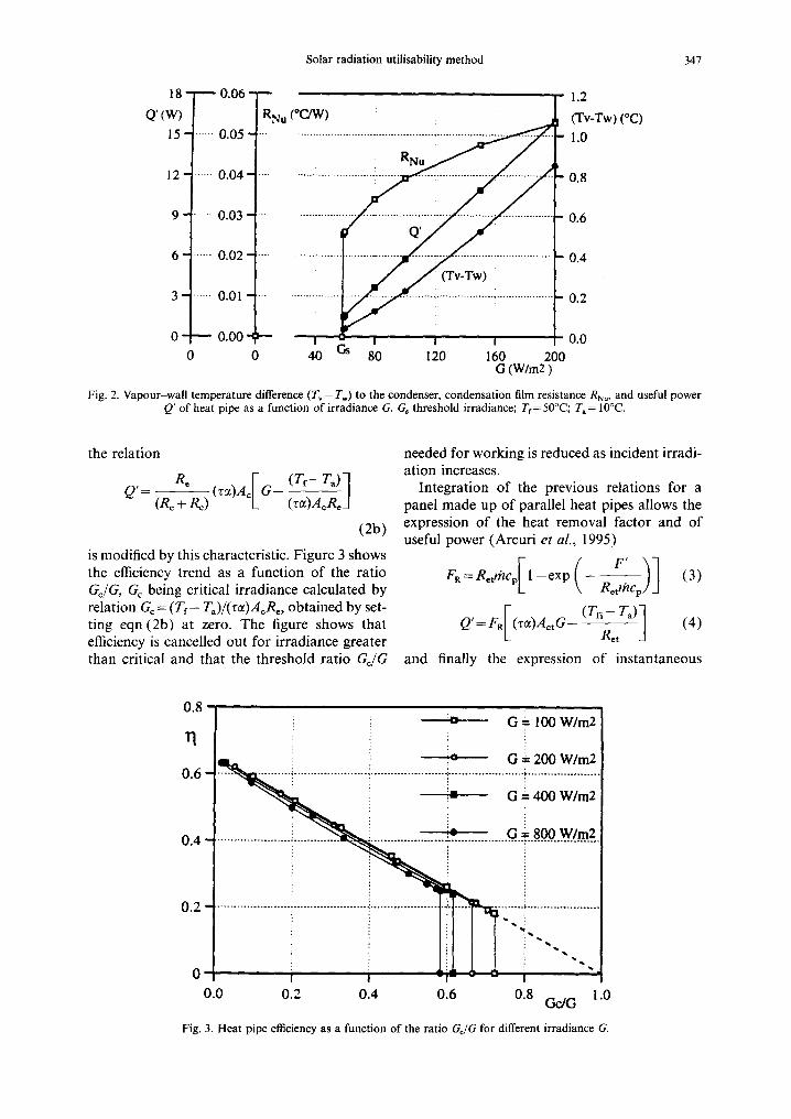
the relation

Q ' - Re [ (Tr-- T~) 1 (R~ + Re) (zc~)A~ G (z~)AeReJ

(2b)

is modified by this characteristic. Figure 3 shows the efficiency trend as a function of the ratio Gc/G, Gc being critical irradiance calculated by relation G¢ = (Tr - Ta)/('ccz)A¢Re, obtained by setting eqn (2b) at zero. The figure shows that efficiency is cancelled out for irradiance greater than critical and that the threshold ratio GdG

needed for working is reduced as incident irradi- ation increases.

Integration of the previous relations for a panel made up of parallel heat pipes allows the expression of the heat removal factor and of useful power (Arcuri et aL, 1995)

R-~t _1 (4)

and finally the expression of instantaneous

0.8 i !n G - 100 W/m2

q

0.6.~ ~ . . i. ' io O : 200 W/m2 . . . . . . . . . . . . . . . i . . . . . . . . . . . . . . . . . . . . . . ".. . . . . . . . . . . . . . . . . . . . . . . i . . . . . . . . . . . . . . . . . . . . . . . i . . . . . . . . . . . . . . . . . . . . . .

~ i i'- G ~- 400 W/m2

0 . 4 _ . i ~ G i 800 W/m2

0 .2 -

!!]li '-- : % •

0.0 0.2 0.4 0.6 0.8 1.0 Gc/G

Fig. 3. Heat pipe efficiency as a function of the ratio Q/G for different irradiance G.


efficiency

rl= FR[(zoo_ (Tfi- Ta)l ~ j (5)

In the foregoing relations Act is the effective collection area of the solar panel, Ret the global thermal resistance for a panel towards the outside, to be calculated should the adiabatic condition move to the outside of the collector tube, with relation (Ret)- 1 = [p/Re +p/(F'Rt)], with p being the number of tubes in a panel, and Rt thermal resistance between the cooling fluid and the outside area through the collector tube of the flow. The efficiency factor of the heat pipe is instead given by the relation F ' = RJ(R~ + R¢).

2. CHARACTERISTICS OF THE PANEL

The thermal analysis carried out with the calculation model has allowed calculation of how, in the hypothesis of step-by-step steady- state collection, thermal resistance Rct through the evaporation surface and resistance to the condenser Rot vary. Results obtained, shown in Fig. 4, show the dependence of resistance Ret on the temperature difference (Tf i -Ta) and on irradiance G, while these variables do not influ- ence resistance Rct.

For a working mass flow of the plant of 0.64 kg/s, that of the experimental plant, the trend of the removal factor FR calculated with eqn (3) is shown in Fig. 5. FR shows a noticeable

dependence on temperature differences (Tf i - Ta), and a more contained dependence on irradiance G. The trend of coefficient FR/Ret, which determines the efficiency curve slope, is shown in Fig. 6 which shows an almost linear dependence on (Tfi-T~) and on G.

The expression of instantaneous efficiency supplied by the manufacturers (Jetten, 1986), should the parameter (Tfi-T~)/G be adopted, is as follows

q =0 .647- [0 .454+7 .1 x 10-4G+5.22

x 10-3(Tfi - Ta) ] (T f i - Ta) G

(6)

A comparison of the foregoing relation with eqn (5) shows that the product FRR~t 1, as predicted by the model, is linearly variable with irradiance G and with temperature difference (Tf i -Ta) , while the intercept with the ordinate axis, represented by the term FR(Z~) is presumed constant. This latter circumstance simplifies the expression of efficiency but gives rise to an error which, evaluated with reference to collection conditions of the plant, is in the order of 2.5%.

The relation, eqn (6), was tested experimentally in the field by data recorded during working of the plant. The correlation obtained, reported in a previous article (Arcuri et al., 1995) supplies an efficiency of 3.2% lower than predicted. This reduction is attributable for a quota of 2% to the union of the panels in series.

. 7 ' ; ; : / i W'm2i

0.6 ~ - - - - - ~ ............. i ............. i ............. ii ......... ""i ' 5 ....... ! ...... i~'~Wim~i ......

0 5 q - ~ - m e t - - - ! ............ ! . . . . i - - i G=6L~_ Wire2

0.4 . . . . . . . . . . . . . i ............. ~ ............ k, ............ i ......

0 . 2 ¸

0 .1 -

0.0

0

iiiiiiiiiiii!iiiiiiiiiiiiiiiiiiiiiiiiiiiiiiiiiiiiiiiiiiiill ........ i ............. i ............ i ............ i . . . . . .

! ! R c t ! i . . . . . . . . i . . . . . . . . . . . . . i . . . . . . . . . . . . . ' . . . . . . . . . . . . . ...... , : : : : _

i i i : i i i I I I I ! ! I

20 40 60 80 100 120 140 160 (Tfi - Ta) (°C)

Fig. 4. Global thermal resistance of a panel to the outside air R~ t and global thermal resistance Ret at the condenser as a function of temperature difference (Tfi- Ta) and for different irradiance G.


0.94

FR

0.92 -

0 . 9 0 -

0 . 8 8 -

0.86 -

0.84

i ' '

C ~--200 W/m 2

.......... ........... .................... ..-+ ......... .....

7. : ~=600 ~ /m 2

iiiiiiiiiii !

0 20 40 60 80 100 120 140 160 180

(Tfi-Ta) (°C)

Fig. 5. Thermal removal factor of the panel as a function of temperature difference (Tfi-- Ta) for different irradiance G.

3.50

, • 3.10 ............................ ~ ....................................................... ; ........... i ........... ~ ......

r¢

u. 2 .70-

2 .30- ! i : : i " :. G~zoow/m2

1.90 - ~ )~- ....

_- o i00 W,m 1.50 I I

0 20 40 60 80 100 120 140 160 (Tfi-Ta) (°C)

Fig. 6. Ratio of the removal factor F R to global thermal resistance R©t as a function of temperature difference (Tri- T,) and of irradiance G.

The above expression of efficiency is valid in the case of normal incidence; use in different conditions requires the correction of the effective transmittance-absorptance product (Tot) by the modifier k = (zot)/(zot),. The trend of k with the angle of incidence 0 is shown in Fig. 7. The trend was obtained by means of experimental tests on an identical panel to that installed by us (Lazzarin et al., 1986). Figure 7 shows that for angles of incidence less than 70 °, coefficient k is greater than that at normal incidence, and this can be attributed to the presence in the

panel of a reflecting screen placed behind the heat pipes. Interpolation of the experimental points for k supplies the expression

k=2.337+2.33 × 1 0 - 3 0 + 1.41 × 10-402

1.337

cos(0.770) (7)

with 0 in degrees. If the concept of critical hourly energy is

used, the relation, eqn (6), allows useful hourly


1.2 : ~ i : i

i . o .... i . . . . . . . . . . . . ! . . . . . . . . . . . .

0 . 8 ..... i ............

0.6 : ...........

0.4 ......

0.2 ---

0.0

0 10 20 30 40 50 60 70 80 O 90

Fig. 7. Trend of the ratio k=(z~)/('r~),, as a function of the angle of incidence 0 for the panel used.

energy to be written as follows

Qh=[0.647k--7.1 × 10-4(Tfi- Ta)](En-Ehc) +

(8)

with E, the incident hourly energy on the panel and Eh¢ the energy lost during working. This latter can be expressed

0.454(Tfi - T~) + 5.22 × 10-3(Tri- T~) z Eh~ = 3.6

0.647k-7.1 × 10-4(Tfi-- T~)

(9)

and depends on the average hourly values of k, Tfi and T~.

The difference (Eh--Eh¢) + is to be computed starting from the threshold of incident energy, which does not coincide with critical energy Eh~ as in traditional collectors, but from Ehs>Eh¢. This condition expresses in energy terms the imbalance Gs> G¢ obtained in the preceding paragraph. The threshold values Ehs have been drawn starting from the analytical expression of Gs obtained by interpolating the irradiance values calculated with the mathematical model in the case of normal incidence. The interpolated values determine the start of collection in the different working conditions of the panel.

The expression obtained of threshold energy Ehs is the following

Ehs = [(0.786 + 0.0142T~) (Tn - Ta)

+ 0.014(Tfi- Ta)2] 3.6 (10)

Figure 8 shows the Ehs trend as a function of temperature difference (Tf i -Ta) for some outside air temperatures Ta, and the Ehs trend calculated with the relation, eqn (9), with k = 1. For ( T f i - T , ) = 8 0 ° C the threshold energy is greater than critical energy by a variable amount of 30-67%.

For angles of incidence different from normal, the previous expression, eqn(10) , should be multiplied by a corrective coefficient kl to be calculated with the relation

kl = 0.040k- 1 + 3.467 - 4.022k + 1.515k 2

( l l )

with k given by eqn (7). Coefficient kl is 1, for k = 1 (0 =0°), and tends to infinity for k tending to zero (0=90°).

The previous relations, eqns(7) and (11), allow the extraction of half-hourly determinant radiation for different angles of incidence, the hourly value of the modifier k, and the corrective coefficient kt, and note the hourly temperature of the outside air and the flow at the inlet, and the calculation of critical hourly energy Ehc with eqn(9) , which quantifies thermal losses, and hourly threshold energy Ehs with the relation, eqn (10), multiplied by k~, which determines the collection interval. Figure 9 shows an example of utilisable energy calculation (Eh--Ehc) + with reference to a perfectly clear day (14 August 1993) and to two different inlet temperatures.

From the hourly utilisable energy it is possible


800 ..O Ehs (Ta =i0 "t2)

~ " 600 . . . . . . . . . . . o . . . . . . . . . . . . . . . . . . . . . . . . . . r..

"~ ' J Ehs (Ta = B 0 C ) . . ~ , / . ~ / J c ~ j - " ~ ' J ~ " " - ~ ~

400 . . . . . . . . . . . . . . ,.c

200 . . . . . . . . . . . . . . . . . . . . . . . . . . . . . . . . . . . . .

0 j !

0 20 40 60 ~ 80 100

( T f i - T a ) ( °C)

Fig. 8. Hourly threshold Eh~ and hourly critical Eh~ energy in the case of normal incidence as a function of temperature difference (Tn- T,) and for different air temperature T,.

1 0 0 0 ' ....

Jt Gs (Tfi = 200°(2) : Gsi(Tfi = IOO°C)

~'~ 8OO- - , Gc (Tfi = 200°~ ) ~ o Gci(Tfi = l~oC)

~ i Z , i ! i i i ~ 6 o 0 -

.................. i !... ................. ' i.. ..........

200 .................. ~ . . . . . . . . . . . . !- ................. ~ ................. i ................. 4 .................. ~ . . . . . . . . . . . i .................. ~ ....... i . i . z _ ~ _ i ! i

0 - - I I

4 6 8 10 12 14 16 18 20 T ime (h)

Fig. 9. Average hourly G (14 August 1993), average hourly threshold G s and average hourly critical G c irradiance, and utilisability energy for two inlet temperatures Tfi.

to c a l cu l a t e the h o u r l y u t i l i s ab i l i t y

(Eh--Go) ÷ ~h = ( 1 2 )

Eh

a n d the a v e r a g e m o n t h l y h o u r useful ene rgy wi th the r e l a t i o n

~ ) h = [ 0 . 6 4 7 k - - 7 . 1 x 10-4(Tfi - Ta]~hEh

(13) SE 57~5-a

T h e a v e r a g e va lues to be c o n s i d e r e d are the m o n t h - h o u r s ; ~h a n d u t i l i s ab i l i ty in the N d a y s o f the m o n t h , g iven by the r e l a t i o n

~h = 1 ~ ( E h - - E h c ) + 1 ~ b h E h (14 )

N /~h N E'h

F i g u r e l 0 shows an e x a m p l e o f a d i s t r i b u t i o n curve a c c u m u l a t e d b y h o u r l y i r r a d i a n c e on the c o l l e c t o r p l a n e a n d o f u t i l i s ab i l i t y ca l cu l a t i on .


.0,

"- 2.5 : ~ i i i i i

2.0 .............. * .............. ~ .............. * .............. ~ ............... , .............. ~ .~. -., ...............

1.5 ..4 .............. ; ......... , ............. ~ ............... ~ .............. ~ . . . . . . . . . . . . . . . . . . . . . . .

,.o i,.!,,i i i - - . 4 - - - ~ ~ . . . . . . . . . . . . . ; . . . . . . . . . . . . . . . i. . . . . . . . . . . . . . . . . . .

fs i ~ ~

0 . 0 . ~ I

0.0 0.1 0.2 0.3 0.4 0.5 0.6 0.7 0.8 0.9 1.0 F rac t ion of t ime in which hou r ly energy is less t h a n Zh

Fig. 10. Cumulative distribution of hourly radiation and utilisability. Surface facing south and inclined to 39.3°: December, 1993, 1-12 a.m.

F i g u r e 11 shows the p lo t t i ng o f the average m o n t h l y h o u r u t i l i sab i l i ty curve wi th reference to a d e t e r m i n e d h o u r a n d the curve l imi t for iden t ica l days . I n this la t te r case u t i l i sab i l i ty is b r u s q u e l y a n n u l l e d w h e n th r e sho ld energy Eh~, r equ i r ed for the w o r k i n g o f the hea t pipe, becomes the same as ava i lab le ene rgy Eh, a c i r c u m s t a n c e t ha t sets co l lec t ion t ime to zero.

T h e eqns (8) a n d (12) were used to ca lcu la te h o u r l y u t i l i sab i l i ty a n d useful h o u r l y energy for

all the h o u r s o f the va r i ous days in a m o n t h . I n these ca l cu l a t i ons ou t s ide air t e m p e r a t u r e was p r e s u m e d to be va r i ab le o n a n h o u r l y basis , whereas flow t e m p e r a t u r e Tfi was p r e s u m e d to be c o n s t a n t o n a da i ly basis a n d the same as tha t o f a s p i r a t i o n f r o m the s torage system. T h e h o u r l y va lues ca lcu la ted in this way were used wi th eqns (13) a n d (14) to ca lcula te the average m o n t h l y h o u r u t i l i sab i l i ty a n d average m o n t h l y h o u r useful energy. F ina l ly , syn thes i s ing eli-

~., 0 .9 .............. , ........... ~ .......... : ........... : .......... *--- 1,;:~.:~-~:[-~2:.; :

0.8

. . . . . . . . . . . . . . . . . . . .

0.6

0.5

0 .4

0.2

0.1 ....

0 .0 i t I

0.0 0.2 0.4 0.6 0.8 1.0 1.2 1.4 1.6 1.8 2.0

Critical radiation ratio Ehe / Eh

Fig. I I. Hourly utilisability for average monthly day (Deccmber 1993) and average monthly hour (11-12 a.m.).


matic data with the average monthly day, average monthly hour utilisability and average monthly day energy were calculated.

3. THE LOOP AND ENERGY COLLECTION

To test the utilisability method working records from an experimental prototype interseasonal storage plant, built at the University of Calabria, were used. The plant supplies the winter heating of a building using only solar energy. Reference is made to a previous article for its working details (Oliveti and Arcuri, 1995). In summary, and for the purpose of this article, the plant has a collection area of 91.2 m 2 achieved by 40 panels and a storage volume of 500m3; its average temperature varies throughout the year from 40 to 80°C. The panels are positioned in three rows, facing south and inclined at 39.3 ° from horizontal (the latitude of the site). A pumping system aspires the flow from the bottom of the accumulator and sends it into the monotube network linking the panels. For the high thermal capacity of the storage system and for thermal stratification problems there, flow temperature at inlet to the panels is kept rigorously constant throughout a collection day.

The plant is equipped with instruments to calculate instantly global balance of its various components and of the whole.

Irradiance G needed for transition of the primary loop in the collection state is calculated with reference to the instantaneous balance equation of the collector's field in steady state: G=mcp (Tfo--Tfi)/rlA, with r/ given by eqn (6) and A the effective collection area of the solar plant. From the measurement of outside air temperature Ta and from temperature Tfi, this latter is presumed to be the same as the mini- mum of the storage system, and setting Tfo = Tfi + 2°C, irradiance G is calculated from the previous relation. The choice of (Tro- Tfi) = 2°C leads to G values which assure a quick and stable start up of collection under the different working conditions that the plant experiences throughout the year.

If the temperature difference during collection becomes less than 1 °C between inlet and outlet to the panels, the pump switches off. This temperature limit was calculated by comparing collected thermal energy with that needed for working of the pump.

In the experimental plant the energy collected from the flow and the incident solar energy are

measured with an error of 1.2 and 2.5%, respectively.

To determine the dynamic behaviour of the collector field one of the standard ASHRAE tests for calculation of the time constant was used (ASHRAE Standard 93-77, 1977). The initially screened collectors field was subjected to a stepped variation of global irradiance of 950 W/m 2, with a flow of 0.64 kg/s, the same as that of the working plant. Details of the experimental test are reported in Arcuri et al. (1995). The outlet temperature trend obtained is shown in Fig. 12 by the natural logarithm of function fl=[Tfo(oo)-Tfo(t)]/[Tfo(OO)-Tfo(O)]. I f the collector field is reduced to a first-order system, the time constant z0, calculated as the time needed in order that the outlet temperature increase related to the maximum increase becomes 0.632, is 6.50 min. The figure shows that the collector field response is more complex and can be set as

f l = l for t<td t

f l = - - 5 . 5 2 5 e 7"12--6.67e t

+8.10 e 3"22fort>td

t

2 . 5 2 (15)

with t expressed in minutes and ta= 1.0 min. The second equation was obtained by extracting the angular coefficients of the straight regression lines and interpolating the points of the curve for t > td. It can be presumed that the response delay time t a and the first time constant of 7.12 min are to be attributed to the heat pipes, the second time constant 2.52 min to the alumin- ium clamps which fix the condensers to the collector tube, and the third of 3.22 min to the steel tube wall and to the water in the collector tube.

Equation (6), which describes the behaviour of the panel in steady state, and eqn (15), which describes the response of the collector field at stepped variation of irradiance, allow us to affirm that the collector field is well-represented by a third-order non-linear model. By means of further elaborations it proved to be, in our case, that the behaviour of the whole collector field is capable of reduction in a first-order model characterised by a delay time ta = 0 min and by a time constant %=6.50 rain, with completely satisfactory results. Figure 13 shows the equiva- lent electric circuit, with Tf average flow temperature, RI global thermal resistance to the outside air, calculated with a quite negligible error by


~ / "r1=7.12 min

~ - 2 - ~ ~

~ -3- ~3=3.22 min ~ -- -4-

e I 'ra=l.0 rain

/ I 0 100 200 300 400 500 600 700 800 900 1000

Time (s)

Fig. 12. Collector field response to a stepped variation of solar global irradiance and time constants for a first-order model (zo) and for a third-order model (~1, ~2, r3). ta, delay time.

?,

Wf

RI~ < C

T~

. (T~-T a)

Ta Fig. 13. Electric circuit of collector field.

the relation obtained from eqn (6)

R 1 = {91.210.454+7.1 × 10-4G +5.22 × 1 0 - 3 ( T f i - Ta)]} - 1

in which global irradiance G, temperatures Tfi

and T a represent daily averages. Resistance R2 traversed by the useful power is expressed by R2=(2mCp )- 1, and the thermal capacity of the panels field by C = z0(Ri- 1 + R~- 1). In the circuit, the constancy of the potential Tfi is assured by an ideal tension generator, while the ideal current generator supplies solar power absorbed by the panels field at every moment. Calculation of currents was obtained applying the principle of superposition, which allows the separate evaluation of the contribution caused by the three forcing causes, represented by the ideal current generator, by the tension and by the starting load of the condenser. The convolution integral was used to test the ascription of solar radiation to different instants.

The model approximates the daily trend of

useful power very well and calculates energy collected with a deviation, compared with values obtained experimentally (less than 1% in the case of clear days, and less than 2.5% in the case of days with highly variable irradiance), but such that it ensures continuity of collection.

The model allows us to study phenomena connected to field inertia during collection. If reference is made to a clear day, the slight variation of solar irradiance is sufficient to produce a reduction of instantaneous power collected compared to steady state, in the case of increasing solar flux (mornings), and a rise in the case of decreasing solar flux (afternoons). The phenomenon can be seen in Fig. 14 in which is shown the daily trend of obtainable power under steady-state conditions, of power calculated with the model, and of experimentally measured power. The same figure also shows the trend of power absorbed by the condenser. A comparison between daily energy levels shows that retaining steady-state collection instant for instant gives rise to a 2.5% overestimation of collected energy. This favour- able result can be attributed to the scarceness of the energy exchanges connected to capacitive effects, compared with energy collected in steady state. Indeed, the use of a mathematical model shows that inlet energy to the condenser on the day under consideration is 2.6% of steady- state energy.

When a day with highly variable solar radiation is considered, capacitive energy exchanges


40 ~ e x p e r i m e n t a l

Q p = ~ l ,~ cp (Tt~-Tn) l dt ffi 838.07 MJ

10 q.:= 22.o~ MJ

lW0 1'1 112 1'3 1'4 1'5 1'6 17 Time (h)

Fig. 14. Daily trend of steady statc power, of rnodcl calculated power, of experimental power and a condenser inlet (20 December 1993). Qa energy absorbed by panels field; Qm useful energy supplied by model; Q useful energy in steady state;

Qp useful cxperimental energy; Qic energy at condenser inlet.

50

kW

40-

30

20

10-

!Qa = 617.32MJ ~[ ~ .'. ill |~

• i i i[~i ~

Q =580.77/~1 !~ .~ ' !

Qp = 507.55 MJ ~ -~,

e x p e r i m e n t a l

A = 9 1 . 2 m2

}

v l'O l', 1'2 ;3 l'5 l'6 Time (h)

Fig. 15. Daily trend of steady-state power, of model calculated power, of experimental power (5 December 1993). Qa energy absorbed by panels field; Qm useful energy supplied by model; Q useful energy in steady state; Qp useful experimental

energy.

are of a markedly greater magnitude. Figure 15 shows instantaneous trends of steady-state power, of measured power, and of that calculated with the mathematical model. Power absorbed by the condenser is shown in Fig. 16. The energy measured on this day is 4.4% less than that collected under steady-state condi-

tions. If a comparison is made on an hourly basis, this difference can reach 30%.

The model supplies 14% of the steady-state absorbed energy for the condenser. If the difference between useful energy in steady state and measured energy is compared with the energy absorbed by the condenser, the results


25-

15-

10-

5-

0-

*5-

-10-

-15 -

-20 -

-25 -

Qic_- 7,.o5 MJ, I I A_- 9,.2-n'-

"---W r I T T T 10 11 12 13 14 15 16

T i m e On)

Fig. 16. Trend of power at condenser inlet (5 December 1993).

show that the condenser returns 69% of the stored energy to the flow, while the remainder is lost to the outside air.

To summarise, it can be stated that in the case of continuous collection, energy effects linked to inertia reduce daily energy in steady- state conditions by not more than 5%.

The use of a collector field model and recorded data has agreed with experimental testing of the irradiance threshold value needed for energy collection. With this aim, the auto- matic main loop switching on and off procedure was isolated for some days and the pump switched on manually before sunrise and off after sunset, so as to include the conditions that determine the start and the end of collecting.

Figure 17 shows an example of irradiance recorded on the collector's surface, and of specific useful power, for the last few hours of a perfectly clear day. The useful power curve was obtained by feeding the panels with water at 59.8°C and with a slightly variable outside air temperature of around 15.5°C. The same figure also traces the instantaneous critical irradiance trends Gc and threshold Gs obtained by the relations, eqns(9) and (10), rewritten in terms of instantaneous powers, taking into account eqns(7) and (11). The trends show that useful power is cancelled out when irradiance on the collector's surface is 77 W/m 2, very close to the calculated threshold of 74 W/m z, and not to the critical 50 W/m z.

These good coincidences have been observed on days in which solar radiation is gradually

variable, without abrupt variations. In other circumstances inertia phenomena modify the irradiance which corresponds to the cancelling out of useful power.

4. USEFUL MONTHLY ENERGY AND EXPERIMENTAL COMPARISONS

The conditions achieved during collection can be summarised in this way: collection area 91.2m 2, mass flow 0.64kg/s, calculated so as to assure energy collection at low irradiance (Oliveti and Arcuri, 1995); variable inlet temperature between 34 and 61°C the same as that available in the bottom part of the accumulator; outside air temperature variable between 2 and 35°C.

The following tables for some typical months show the results of a comparison between monthly hour useful energy ~ Qh calculated by the utilisability method, and monthly hour useful energy ~ Qh,p measured in the plant. In order to take into account that the procedure employed for starting up and shutting down collection needs greater irradiance than that foreseen for the utilisability method, useful energy Q~ starting from the threshold used in the working of the plant was also calculated using the utilisability method.

Comparisons between measured energy E Qh,p and those preceding )-" Q* therefore show effects produced by inertia during energy collection, while comparisons between energies


300 I'

W/m2 L

25o-i. . . . . . . . . . . . . . . . . . . . . . . . . . . . . . . . . . . . . . . . . . . . . . . . . . . . . . . . . . . . . . . . . . . . . . . . . . . . . . . . . . . . . . . . . . . . . . . . . . . . . . .

" ° ................................... ..................................................................... I

O ~ . . . . . . . . . . . .

-50 i , , I

15.50 15.75 16.00 16.25 16.50 16.75 T ime (h)

Fig. 17. Stopping of collection on a clear day (3 November 1993); G irradiance on collectors surface; Q~/A specific useful power; G~ threshold irradiance; G c critical irradiance.

Y' Q~ and ~ Qh show losses caused by the reduct ion o f the collection time, because o f the delay in starting up and the anticipation in shutt ing down.

Table 1 summarises the results obtained in August , 1993, characterised by perfectly clear days (monthly clearness index 0.622) and by cont inuous collection. A compar ison o f the hourly values o f the ratio ~ Qh,p/E Q* between the corresponding hours, before and after midday, show the inertia effect o f the system on energy collection. The ratio ~ Q*/~ Qh for the regularity o f radiat ion trend in all the days o f the mon th quantifies the losses connected to start ing up in the first hour o f collection and the losses connected to shutt ing down in the last hour. Measured energy in the whole mon th

is 2.6% less than that predicted by the utilisability method. This reduct ion can be at tr ibuted to inertia phenomena for 2.2% and to the reduction in collection time for the remaining 0.4%.

Table 2 shows results obtained in December, 1993 (monthly clearness index 0.338) in the course o f which radiat ion was highly variable, with collection interruptions on several days and also with successive starting up o f the plant. Overall, energy collected was less than 9.6% of that predicted by calculation. This reduct ion can be at tr ibuted to inertia phenomena for 4.7% and to starting up and shutting down o f the plant for 4.9%.

Finally, Table 3 shows results obtained in March 1994 (monthly clearness index 0.509), characterised by an availability o f solar energy

Table 1. Utilisability and average monthly hour useful energy (August 1993): comparisons with experimental data; Tn =41.6-54.1°C

2e~ 2(e~-eho) + Ee~ EQ.., Y ~ Ore ,kJ/m') (kJ/m', ~, (kJ/m') (kJ/m ~) (kJ/m')~z~Q~.hp/ ~.l,/ ~ /

7 10 977 5382 0.490 1589 162 187 0.102 0.866 0.118 8 30 836 28 339 0.919 17 104 14 966 17 104 0.875 0.875 1 9 53445 51 540 0.964 35 512 33 133 35 512 0.933 0.933 1

10 73 207 71 565 0.978 49 860 47 267 49 860 0.948 0.948 1 11 87 272 85 721 0.982 58 194 55 575 58 194 0.955 0,955 1 12 96 711 95 198 0.984 62 815 62 375 62 815 0.993 0.993 1 13 98 106 96 616 0.985 63 885 63 693 63 885 0.997 0,997 1 14 88 840 87 414 0.984 59 539 55 905 59 539 0.939 0.939 1 15 77400 75 914 0.981 53 055 50 296 53 055 0.948 0.948 1 16 57446 55 905 0.973 38607 37 989 38 607 0.984 0.984 ! 17 32 712 30 844 0.943 18 586 21 319 18 586 1.147 1.147 1 18 12 614 8497 0.674 2481 6560 1949 2.644 3.366 0.785

719 566 692 935 0.963 461 227 449 240 459 293 0.974 0.978 0,996

358

Table 2.

G. Oliveti and N. Arcuri

Utilisability and average monthly hour useful energy (December 1993): comparisons with experimental data; Tn = 57.0-48.3°C

Ore (kJ/m 2) (kJ/m 2) ~h (k J/m~) (k J/mz) (k J/m2)

9 14 373 10 412 0.724 6974 2334 6866 0.335 0.340 0.985 10 27 240 22 721 0.834 15 413 13 263 14 895 0.861 0.890 0.966 11 34 717 29 650 0.854 19 786 17 748 18 840 0.897 0.942 0.952 12 38 989 34 303 0.880 22 555 20 515 21 722 0.910 0.944 0.963 13 37 137 33 016 0.889 21 827 21 176 20 585 0.970 1.029 0.943 14 31 377 27 252 0.869 18 404 17 589 17 220 0.956 1.021 0.936 15 21 909 18 244 0.833 12 485 12 694 11 912 1.017 1.066 0.954 16 10 196 7101 0.696 4689 5108 4130 1.089 1.237 0.881

215 938 182 699 0.846 122 133 110 427 116 170 0.904 0.951 0.951

Table 3. Utilisability and average monthly hour useful energy (March 1994): comparisons with experimental data; T f i = 34.8-36.1 °C

•

Ore (kJ/m z ) (kJ/m 2) ~h (kJ/m 2 ) (kJ/m z ) (kJ/m:) ~ Q h E Q* Eeh 7 2270 J2 0.023 15 8 14 634 11 924 0.815 7111 2764 6619 0.389 0.418 0.931 9 32 746 30 329 0.926 20 824 17 147 20 073 0.820 0.854 0.964

10 52 139 49 981 0.959 34 697 31 096 34 415 0.900 0.904 0.992 11 67 089 65 017 0.969 43 803 41 016 43 526 0.940 0.942 0.994 12 68 359 66 288 0.970 42 978 43 096 42 541 1.000 0.987 0.990 13 67 359 65 397 0.971 42 240 41 947 41 999 0.990 0.999 0.994 14 62 773 60 942 0.971 40 959 38 435 40 628 0,940 0.946 0.992 15 51 350 49 520 0.964 34447 32 236 34 182 0.940 0.943 0.992 16 36 061 34 238 0.949 23 793 22 996 22 884 0.970 1.005 0.962 17 18 675 16 651 0.892 10 326 11 399 9793 1.100 1.163 0.908 18 4318 1701 0.394 556 1481 2.660

477 775 452040 0.946 301 749 283 613 296 660 0.940 0.956 0.983

which can be taken to be intermediate with reference to the two previously cited extremes. Collected energy was 6.0% less than predicted; this reduct ion can be a t t r ibuted to inertia for 4.3% and to the higher threshold flux needed for working for 1.7%.

It should be noted that the hour ly t rend of the ratio ~ Qh,p/~. Q~, which quantifies the inert ia effects, is quali tat ively identical for the three mon ths considered.

Useful energy was also calculated start ing f rom climatic data relative to the average month ly day, supposing the collector field to be fed with a cons tan t inlet temperature and at average value, and as far as the panel characteristics are concerned, average month ly hours of modifier k, correct ion factor kl, threshold energy and critical energy were considered. The results ob ta ined can be summarised as follows.

In Augus t and March, average threshold energy E~hd) needed at different hours for collec- t ion was always less than incident energy on panel E~h a) and, moreover, the critical ratio E~hd2/E~h a) was very slight, if the first and last hours are excluded. For this circumstance, in bo th mon ths considered, useful energy calcu-

lated is coincident, with deviat ions of less than 1% with that obta ined by average month ly hours.

For December the preceding difference was greater. The results are shown in Table 4, in which hour ly threshold energy E ~d~, critical energy E~d2, and threshold energy in working condi t ions E ~ d~ are also shown. The e l iminat ion of daily variabil i ty gives rise to a 2.7% reduct ion of useful energy calculated. Experimental ly measured energy is less than 7.1% of calculated energy, whereas in the foregoing evaluation, it was 9.6%. If useful energy is calculated with reference to the threshold energy needed for working, a result of 1.3% less than the experi- menta l one is obtained, while the effect at t r ibut- able to a reduct ion in collection hours because of a higher energy threshold E ~ d~ is 8.3%.

5. CONCLUSIONS

The results obta ined through experimental and numerica l analysis of the collector field highlight the goodness of the utilisability method for the predict ion of energy gathering for evacuated heat pipe panels. The numerical


Table4. Utilisability and useful energy (December 1993, average monthly day): comparisons with experimental data; t,i=52.2oc

Ore (kJ/m 2) (kJ/m 2) (kJ/m 2) t~h (kJ/m 2) (kJ/m 2) (kJ/m z) (kJ/m 2)

8 51 257 191 529 9 464 229 168 0.638 198 75 528 0.379 10 879 223 162 0.816 488 428 524 488 0.877 11 - 1120 221 160 0.857 642 573 517 642 0.893 12 1258 218 156 0.876 725 662 510 725 0.913 13 1198 213 152 0.873 692 683 505 692 0.987 14 1012 208 147 0.855 584 567 503 584 0.971 15 707 205 144 0.796 385 409 502 385 1.062 16 329 211 149 0.547 119 165 503 1.387 17 12 212 151 504

7030 0.815 3833 3562 3516 0.929

inves t iga t ion into heat tube work ing has shown tha t in col lect ion cond i t ions achieved in the p lan t the effect o f va r ia t ion in the thermal r emova l fac tor FR no t a l lowed for by the efficiency curve is in the o rde r o f 2.5%, and tha t hour ly th resho ld energy needed for the work ing o f the heat tube can exceed cri t ical hour ly energy ob t a ined th rough the efficiency curve by 67%. A c o m p a r i s o n with the ins t an taneous t rend o f measu red power has under l ined tha t the dynamic behav iou r o f the field is capab le o f reduc t ion to a f i rs t -order l inear model , wi th an er ror , c o m p u t e d on dai ly col lected energy, tha t does not exceed 2.5%. The mode l a l lows us to test the effects p r o d u c e d by iner t ia on dai ly energy col lect ion, effects tha t c o m p a r e d with every ins tant s teady-s ta te col lect ion p r o d u c e d in the o rde r o f 2% energy reduc t ion in the case o f clear days, and 5% in the case o f days with grea t r ad i a t i on var iabi l i ty .

Energy compar i sons on a mon th ly basis between exper imenta l values and pred ic t ions carr ied out by the average m o n t h l y hour uti l isabi l i ty me thod show tha t energy reduct ion owing to capaci t ive effects vary f rom 2.2% ( A u g u s t ) to 4.9% (December ) , thus conf i rming the results ob ta ined with the model , whereas the quo ta a t t r i bu tab le to the decrease in col lect ion time, varies f rom 0.4% ( A u g u s t ) to 4.9% (December ) .

I f the compa r i son of measu red energy is car r ied out with energy ca lcu la ted by average m o n t h l y day ut i l isabi l i ty , the foregoing results are conf i rmed for the col lect ion condi t ions achieved, except in D e c e m b e r when the decrease in col lect ion hours reduced useful energy by 8.3%.

Fo r the scarceness o f effects p r o d u c e d by iner t ia o f the system, a cor rec t ion o f useful energy pred ic ted by the m e t h o d does not seem proposab le . However , a ref inement o f the

5E 57-5~C

m e t h o d can be ob ta ined by ca lcula t ing the energy s tar t ing f rom threshold values needed for the effective work ing o f the plant , especial ly for those mon ths with grea t var iab i l i ty o f solar rad ia t ion .

NOMENCLATURE

A effective area collection of the panel's field, m 2 A c effective area collection of the heat pipe, m 2 Act effective area collection of the solar panel, m 2

C heat capacity in the model of the panel's field, W/°C % specific heat of the water, kJ/kg °C E h total hourly on tilted panel energy, kJ/m 2

Eho critical hourly panel energy, kJ/m 2 E_h, hourly threshold energy for working panel, kJ/m 2 Eh average monthly hour on tilted panel energy, kJ/m 2

~h d) hourly energy on tilted panel for average monthly day, kJ/m 2

~h~J critical hourly energy for average monthly day, kJ/m 2

E~ ~ hourly threshold energy for average monthly day, kJ/m 2

E~s hourly threshold energy required for the working of the plant, kJ/m 2

E~hJ a~ hourly threshold energy for average monthly day required for the working of the plant, k J / m 2

F' efficiency factor of the heat pipe F R panel heat removal factor G instantaneous global (or average hourly) tilted surface

i r r ad i ance , W / m 2 Gc average hourly critical irradiance, W / m 2 G, average hourly threshold irradiance by working heat

pipe, W,/m 2 k incident angle modifier

kl corrective coefficient of hourly threshold energy m mass flow rate, kg/s N number of days in the month p number of heat pipes in a panel

Q' instantaneous useful thermal power output panel, W Qh useful hourly energy per unit area panel, kJ/m 2 Qh average monthly hour useful energy, k J / m 2 Q~' useful hourly energy computed starting for the thresh-

old energy E~'~ required for the working of the plant, kJ/m 2

Q~h d~ useful hourly energy for average monthly day, kJ/m 2 Q~,td~ useful hourly energy for average monthly day com-

puted starting threshold energy E~h~ d~, kJ/m 2 Qh.p useful hourly energy measured in the plant, kJ/m 2


Qh.p average monthly hour useful energy measured in the plant, kJ/m 2

P~ global thermal resistance at the heat pipe condenser, °C/W

R~t global thermal resistance for a panel at the condenser, °C/W

R c global thermal resistance between the outside surface of the evaporation zone of the heat pipe and the outside, °C/W

Ret global thermal resistance for a panel towards the outside, °C/W

RNu heat pipe condensation film resistance heat pipe, °C/W R t global thermal resistance between the cooling flow

and the outside through the collector tube, °C/W R, global thermal resistance in the model of the panel

field towards the outside, °C/W R 2 global thermal resistance in the model of the panel

field for the calculation of useful power, °C/W t time, min

t d delay time, min T, outside air temperature, °C Tf cooling flow temperature, °C Tr average cooling flow temperature in the panel field, °C

Tfi inlet cooling flow temperature, °C Tfo outlet cooling flow temperature, °C Tv vapour temperature, °C Tw condenser wall temperature, °C

Greek letters

r/ panel instantaneous efficiency ~h hourly utilisability ~bh average monthly hour utilisability

~b~h d~ hourly utilisability for average monthly day 0 angle of incidence between direct solar radiation and

the normal to the panels surface, degrees z time constant, min

(rot) effective transmittance-absorptance product

REFERENCES

Arcuri N., Cucumo M. and Oliveti G. (1995) Determinazi- one sperimentale dell'efficienza istantanea di un campo di collettori solari a tubi di calore. Condizionamento dell'aria, riscaldamento e refrigerazione, Luglio, pp. 707-715.

ASHRAE Standard 93-77 (1977) Methods of testing to determine the thermal performance of solar collectors. American Society of Heating, Refrigeration, and Air Conditioning Engineers, New York.

Cucumo M., Marinelli V. and Oliveti G. (1994) Ingegneria Solare. Pitagora editrice, Bologna.

Cucumo M. and Marinelli V. (1983) Thermal analysis and working limits of heat pipe solar collectors. European two phase flow group meeting 1984, paper B/5, Rome, June.

Duffle J. A. and Beckman W. A. (1991) Solar Engineering of Thermal Processes, 2nd edition. Wiley, New York.

Jetten R. (1986) Philips, Eindhoven, The Netherlands, pri- vate communication.

Klein S. A. (1978) Calculation of fiat-plate collector utilizability, Solar Energy 21, 393-402.

Klein S. A. and Beckman W. A. (1984) Review of solar radiation utilizability. Trans. ASME. J. Solar Energy Eng. 106, November.

Liu B. Y, H. and Jordan R. C. (1963)The long-term average performance of flat-plate solar energy collectors. Solar Energy 7, 53-74.

Lazzarin R., Schibuola L. and Grinzato E. (1986) La prova dei collettori solaria tubi evacuati risultati sperimentali. Energie Alternative HTE, anno 8, 413-427.

Oliveti G. and Arcuri N. (1995) Prototype experimental plant for the interseasonal storage of solar energy for the winter heating of buildings: description of plant and its functions. Solar Energy 54, 85-97.

Ribot J. and McConnel R. D. (1983) Testing and analysis of a heat-pipe solar collectors. Trans. ASME. J, Solar Energy Eng. 105, November.

Solar radiation utilisability method in heat pipe panels

Documents

Transcript of Solar radiation utilisability method in heat pipe panels