A Heuristic Approach for Determining Lot Sizes and Schedules Using Power-of-Two Policy
18
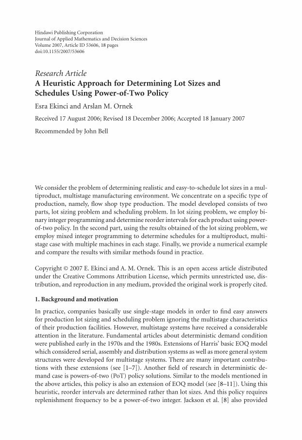
Hindawi Publishing Corporation Journal of Applied Mathematics and Decision Sciences Volume 2007, Article ID 53606, 18 pages doi:10.1155/2007/53606 Research Article A Heuristic Approach for Determining Lot Sizes and Schedules Using Power-of-Two Policy Esra Ekinci and Arslan M. Ornek Received 17 August 2006; Revised 18 December 2006; Accepted 18 January 2007 Recommended by John Bell We consider the problem of determining realistic and easy-to-schedule lot sizes in a mul- tiproduct, multistage manufacturing environment. We concentrate on a specific type of production, namely, flow shop type production. The model developed consists of two parts, lot sizing problem and scheduling problem. In lot sizing problem, we employ bi- nary integer programming and determine reorder intervals for each product using power- of-two policy. In the second part, using the results obtained of the lot sizing problem, we employ mixed integer programming to determine schedules for a multiproduct, multi- stage case with multiple machines in each stage. Finally, we provide a numerical example and compare the results with similar methods found in practice. Copyright © 2007 E. Ekinci and A. M. Ornek. This is an open access article distributed under the Creative Commons Attribution License, which permits unrestricted use, dis- tribution, and reproduction in any medium, provided the original work is properly cited. 1. Background and motivation In practice, companies basically use single-stage models in order to find easy answers for production lot sizing and scheduling problem ignoring the multistage characteristics of their production facilities. However, multistage systems have received a considerable attention in the literature. Fundamental articles about deterministic demand condition were published early in the 1970s and the 1980s. Extensions of Harris’ basic EOQ model which considered serial, assembly and distribution systems as well as more general system structures were developed for multistage systems. There are many important contribu- tions with these extensions (see [1–7]). Another field of research in deterministic de- mand case is powers-of-two (PoT) policy solutions. Similar to the models mentioned in the above articles, this policy is also an extension of EOQ model (see [8–11]). Using this heuristic, reorder intervals are determined rather than lot sizes. And this policy requires replenishment frequency to be a power-of-two integer. Jackson et al. [8] also provided
-
Upload
independent -
Category
Documents
-
view
0 -
download
0
Transcript of A Heuristic Approach for Determining Lot Sizes and Schedules Using Power-of-Two Policy
Hindawi Publishing CorporationJournal of Applied Mathematics and Decision SciencesVolume 2007, Article ID 53606, 18 pagesdoi:10.1155/2007/53606
Research ArticleA Heuristic Approach for Determining Lot Sizes andSchedules Using Power-of-Two Policy
Esra Ekinci and Arslan M. Ornek
Received 17 August 2006; Revised 18 December 2006; Accepted 18 January 2007
Recommended by John Bell
We consider the problem of determining realistic and easy-to-schedule lot sizes in a mul-tiproduct, multistage manufacturing environment. We concentrate on a specific type ofproduction, namely, flow shop type production. The model developed consists of twoparts, lot sizing problem and scheduling problem. In lot sizing problem, we employ bi-nary integer programming and determine reorder intervals for each product using power-of-two policy. In the second part, using the results obtained of the lot sizing problem, weemploy mixed integer programming to determine schedules for a multiproduct, multi-stage case with multiple machines in each stage. Finally, we provide a numerical exampleand compare the results with similar methods found in practice.
Copyright © 2007 E. Ekinci and A. M. Ornek. This is an open access article distributedunder the Creative Commons Attribution License, which permits unrestricted use, dis-tribution, and reproduction in any medium, provided the original work is properly cited.
1. Background and motivation
In practice, companies basically use single-stage models in order to find easy answersfor production lot sizing and scheduling problem ignoring the multistage characteristicsof their production facilities. However, multistage systems have received a considerableattention in the literature. Fundamental articles about deterministic demand conditionwere published early in the 1970s and the 1980s. Extensions of Harris’ basic EOQ modelwhich considered serial, assembly and distribution systems as well as more general systemstructures were developed for multistage systems. There are many important contribu-tions with these extensions (see [1–7]). Another field of research in deterministic de-mand case is powers-of-two (PoT) policy solutions. Similar to the models mentioned inthe above articles, this policy is also an extension of EOQ model (see [8–11]). Using thisheuristic, reorder intervals are determined rather than lot sizes. And this policy requiresreplenishment frequency to be a power-of-two integer. Jackson et al. [8] also provided

2 Journal of Applied Mathematics and Decision Sciences
some interesting theoretical discussions on the optimal solution resulted from the PoTpolicy. That is, the optimal objective function value under PoT policy is within 6% errorrange.
There exist a number of extensions of PoT policy in literature. Capacitated version ofthe model is considered in [8] and joint replenishment problem in [12], whereas Roundy[13] and Muckstadt and Roundy [14] propose solutions for one-warehouse, multire-tailer problem. Moreover, extensions on finite production rate and backlogging problemscan be found in [15, 16]. Especially related with the economic lot-scheduling problem(ELSP), there exist a number of articles on the topic of cyclic schedules (see [17–20]).Cyclic schedules are a generalization of common cycle schedules in which the cycle timeof a product is an integer multiple of a basic period. PoT policy on ELSP is a special typeof cyclic schedules. Yao and Elmaghraby [21] studied a single-stage ELSP problem andlater Lee and Yao [22] proposed a global optimum search method for the joint replenish-ment problem (JRP) under PoT policy. Ouenniche and Boctor [11] presented a new andefficient heuristic to solve multiproduct, multistage, economic lot-sizing problem wheresequencing, lot sizing, and scheduling decisions are made for several products manufac-tured through several stages in a flow-shop environment so as to minimize the sum ofsetup and inventory holding costs while a given demand is fulfilled without backlogging.Ouenniche et al. [23], on the other hand, studied the impact of sequencing decision ontotal cost.
The objective of this study is to develop a heuristic approach to find reorder inter-vals based on PoT policy and consequently lot sizes for items to be produced, and thenassign and schedule these production lots in a multistage, multimachine production envi-ronment. We consider a specific type of production, namely, flow shop type productionwhich is a serially structured multistage system that exists in industries like paint pro-duction, food canning, or beverage bottling companies. These types of processes mayhave some technical restrictions. In addition, the waiting time of in-process invento-ries between stages should be minimal since waiting time can cause product deteriora-tion.
We consider the problem in two parts: (i) reorder interval (lot size) determination and(ii) assignment and scheduling problem. In the first part, we solve a constrained ELSPassuming the production system as a single stage. The production rate is the rate of thebottleneck stage. Nonlinear structure of the model is modified to mixed-integer program-ming (MIP) form and MIP is solved to determine the reorder intervals as integer mul-tiples of power-of-two multipliers by minimizing the objective function which consistsof inventory and setup costs. Basically, the model proposed in the first part differs fromthe classical unconstrained ELSP model developed by Yao and Elmaghraby [21] in thatit considers upper and lower limits on production lot sizes as well as lot-size-dependentsetup costs in the formulation.
In the second part, the assignment and scheduling problem is solved using an MIPbased on an approach developed in [11] but with the additional condition of multiplemachines in each stage. An optimal schedule is achieved with the assumption of givenproduction sequence. In practice, the production sequence is generally determined bysome technical criteria.

E. Ekinci and A. M. Ornek 3
The rest of the paper is organized as follows. Section 2 considers the model devel-opment, that is, determining optimum reorder intervals and lot sizes under PoT policyfor multiproducts subject to operational constraints and then scheduling those lots in amultistage and multimachine environment. Then Section 3 presents a numerical exam-ple and compares the results obtained with similar methods found in practice. Finally, inSection 4, we present our conclusions.
2. The model development
Here, we first present the classical ELSP, then add technical constraints based on the spe-cific production environment. Later, we develop the formulation considering the lot sizedependent setup costs. In the second part, we assign and schedule these production lotsto stages and machines using an MIP model. The model is designed for multistage, mul-tiproduct problem, with multiple machines in each stage.
2.1. Determining optimum lot sizes under power-of-two policy. We define the nota-tion as follows. Additional notation will be defined as necessary.
Indices:(i) i= product index (i= 1, . . . ,n),(ii) y = container type (y = 1, . . . ,z). A container is a receptacle for holding products.
Parameters:(i) Ai = setup cost for product i,(ii) Aiy = setup cost for product i dependent on container type y,(iii) λi = demand rate for product i, constant and continuous,(iv) hi = holding cost per unit time for product i,(v) pi = finite production rate for product i,(vi) si = setup time for product i,(vii) ρi = λi/pi,(viii) Cy = upper-volume (lot-size) limit of container type y,(ix) TL = technical limit showing the minimum lot amount for a machineto work effectively,
Decision variables:(i) ki = power-of-two multiplier for product i (ki = 1,2,4, . . . ,2mi ; mi ∈ {0,1,2, . . .}),(ii) B = basic period,(iii) xi j = the valid power-of-two multiplier (2 j) for product i, xi j = {0,1}.
The limits of the index j will be determined later.The following assumptions are made in the first part of the model.
(1) No backlogging is allowed.(2) The ordering decision for each product is given in every constant time interval
which is a power-of-two (PoT) multiple of a basic period B, that is, kiB.(3) The basic period B may be specified as a shift, a day, or a week, and so forth.(4) The finite production rate is that of the bottleneck stage.

4 Journal of Applied Mathematics and Decision Sciences
Unconstrained economic lot-scheduling problem (ELSP) PoT problem formulated in[21] is as follows:
MinTC(B,{ki})=
n∑
i=1
Ai
kiB+hi2λi(1− ρi
)kiB (2.1a)
subject to ki = 2mi ; mi ∈{
0,1,2, . . .}. (2.1b)
ELSP (PoT) is formulated as a nonlinear integer program. The objective function (2.1a)is the sum of average annual costs of setup and carrying inventory. In spite of the fact thatthe objective function (2.1a) is a nonlinear one, for a given value of B, the model can berestated as a linear binary integer programming (BIP) model. ki and its reciprocal can bewritten in binary expansion [21]:
ki =vi∑
j=0
2 jxi j = 20xi0 + 21xi1 + ···+ 2vixivi , (2.2)
k−1i =
vi∑
j=0
2− jxi j = 20xi0 + 2−1xi1 + ···+ 2−vixivi , (2.3)
vi∑
j=0
xi j = 1, ∀i, (2.4)
where vi is a nonnegative integer and 2vi ∗B is an upper bound on ki.
We add upper and lower bound constraints on lot sizes to the above model relatedwith the specific production type. For a single type of container, constrained ELSP (PoT)becomes
MinTC(B,{ki})=
n∑
i=1
Ai
kiB+hi2λi(1− ρi
)kiB (2.5a)
subject to ki = 2mi ; mi ∈{
0,1,2, . . .}
, (2.5b)
λikiB ≥ TL, ∀i, (2.5c)
λikiB ≤ C, ∀i. (2.5d)
In the above formulation, constraint (2.5c) indicates the minimum technical limit foreffective working of the machine. In addition, constraint (2.5d) sets the upper limit forlot size according to the container restrictions. Using (2.2)–(2.4), the BIP model can be
E. Ekinci and A. M. Ornek 5
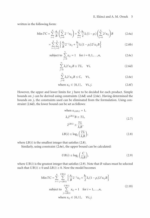
written in the following form:
MinTC =n∑
i=1
Ai
B
( vi∑
j=0
2− jxi j
)
+n∑
i=1
hi2λi(1− ρi
)( vi∑
j=0
2 jxi j
)
B (2.6a)
=n∑
i=1
vi∑
j=0
{Ai
B2− jxi j +
hi2λi(1− ρi
)2 jxi jB
}(2.6b)
subject tovi∑
j=0
xi j = 1 for i= 0,1, . . . ,n, (2.6c)
vi∑
j=0
λi2 jxi jB ≥ TL, ∀i, (2.6d)
vi∑
j=0
λi2 jxi jB ≤ C, ∀i, (2.6e)
where xi j ∈ {0,1}, ∀i, j. (2.6f)
However, the upper and lower limits for j have to be decided for each product. Simplebounds on j can be derived using constraints (2.6d) and (2.6e). Having determined thebounds on j, the constraints used can be eliminated from the formulation. Using con-straint (2.6d), the lower bound can be set as follows:
when xi,LB(i) = 1,
λi2LB(i)B ≥ TL,
2LB(i) ≥ TL
λiB,
(2.7)
LB(i)≥ log2
(TL
λiB
), (2.8)
where LB(i) is the smallest integer that satisfies (2.8).Similarly, using constraint (2.6e), the upper bound can be calculated:
UB(i)≤ log2
(C
λiB
), (2.9)
where UB(i) is the greatest integer that satisfies (2.9). Note that B values must be selectedsuch that UB(i)≥ 0 and LB(i)≥ 0. Now the model becomes
MinTC =n∑
i=1
UB(i)∑
j=LB(i)
{Ai
B2− jxi j +
hi2λi(1− ρi
)2 jxi jB
}
subject toUB(i)∑
j=LB(i)
xi j = 1 for i= 1, . . . ,n,
where xi j ∈ {0,1}, ∀i, j.
(2.10)
6 Journal of Applied Mathematics and Decision Sciences
In case the setup costs vary with container sizes, we modify the objective function asfollows. The lower limit (TL) is the same for all container sizes. But for the upper limits,each container has a different limit, that is, Cy . Hence, the upper bounds for differentcontainer sizes can be calculated using (2.9), that is, replacing C value by Cy values. Thus,the average annual setup cost term
n∑
i=1
UB(i)∑
j=LB(i)
{Ai
B2− jxi j
}(2.11)
for different containers now becomes
n∑
i=1
z∑
y=1
{ UB(i,y)∑
j=LB(i,y)
{Aiy
B2− jxi j
}}
. (2.12)
Another point to be emphasized is the minimum total cost functions which will becalculated for discrete B values. B would be multiples of a shift, a day, a week, or a month.Moreover, the search section of B—the highest and the lowest values—should be con-sidered. Value found in common cycle approach is the upper bound on the value of B[21]:
Tcc =max
⎧⎨
⎩
√√√√ 2
∑ni=1Ai∑n
i=1hiλi[1− ρi
] ,
∑ni=1 si
1−∑ni=1 ρi
⎫⎬
⎭ . (2.13)
A lower bound on the value of B can be obtained using rotation cycle policy [21]:
Trc =maxi
{(1 + ρi
)si}. (2.14)
This interval from the upper to lower bounds covers a feasible range of B. For example,feasible region can be between 1 day and 14-day length. Then the model can be run forbasic periods of 1 day, 2 days and upto 14 days. Another simplification in this part is that,the basic periods that are power-of-two multiples of other feasible basic periods give thesame optimal value for the model. Again in the same example of 1-day to 14-day feasibleregion of basic period, one can run the model for only 1-day, 3-day, 5-day, 7-day, 9-day,11-day, 13-day basic period. The optimal value will be the same for 1, 2, 4, 8, and for 3,6, 12, and for 5, 10 and similarly for 7, 14 days. The theorem given in [21] can be used toshow that the program yields the same solution for a power-of-two multiple of a feasiblebasic period. However, in our case, there exist upper and lower limits for container typesand when we change the basic period B to 2B, then the lower bound decreases by 1 asfollows:
LB(i)≥ log2
(TL
λiB
)=⇒ log2
(TL
λi2B
)= log2
(TL
λiB
)− log2
(12
)= log2
(TL
λiB
)− 1
=⇒ LB(i)− 1≥ log2
(TL
λiB
)− 1.
(2.15)
E. Ekinci and A. M. Ornek 7
But, if one or more products have 0 as a lower limit for B, then the theorem cannotbe used. However, none of the products can have lower limit as −1 for 2B, since thereorder interval cannot be 2−1∗ (2B). In this case, the limits of the containers should becalculated for 2B and the integer values greater than or equal to 0 should be chosen as j.Thus, the program should be executed for 2B.
The results obtained in this part giving the minimum cost for a specific basic periodwill be used in the following section. An MIP is developed to assign and schedule thelots so found to a multistage multimachine production system. Here, we assume that themachines at each stage are identical and the production sequence is predetermined bysome technical criteria.
2.2. Assigning and scheduling the lot-sizing problem in a multistage, multimachineenvironment. The lot sizes obtained in the first part will be assigned to basic periods,and for each basic period feasible schedules will be determined by an assignment proce-dure based on a method given in [11]; however, nonlinear program used in schedulingwould be modified in order to support multimachine environment. Also, note that theproduction sequence of the jobs (products) is predetermined by the technical personnel.
Using the solutions of the first part, global cycle length becomes TG = K ∗ B, whereK =max{ki}. Let Pt denote the set of products to be produced during the tth basic periodof the global cycle. For a calculated value of K in the first part, we have to assign productsto the subsets, P1,P2, . . . ,PK . For example, for a product i, let ki be 2 and global cyclelength is 4 basic periods. Then product i has to be produced either in the first and thirdbasic periods or in the second and fourth basic periods. Let πi be the processing time ofproduct i:
πi = kiλiB
pi, ∀i. (2.16)
Given a vector of multipliers (ki; i = 1, . . . ,n), the purpose of the following heuristicprocedure is to try to find a feasible assignment of products to basic periods (P1,P2, . . . ,PK ). The procedure starts by sorting the products in ascending order of ki, and within theproducts having the same multiplier ki, in descending order of processing time. Compar-ison between processing times can be done using the term ρ∗i below:
ρ∗i =kiλipi
. (2.17)
As ρ∗i gets larger, the processing time also becomes larger, because ρ∗i times B is thereal process time of the product i.
Then, each product i is assigned to the first basic period l, satisfying (2.18), within thefirst ki periods of the global cycle that yet have the smallest summation of ρ∗i s that areassigned in that basic period Pt,
mint<ki
(∑
u∈Pt
kuλupu
)
+kiλipi
< 1, t = l, l+ ki, l+ 2ki, . . . , l+K − ki. (2.18)
8 Journal of Applied Mathematics and Decision Sciences
Note that sorting the products in ascending order of ki, and within the products havingthe same multiplier ki in the descending order of ρ∗i allows us to assign first the productsthat require more production time, that is, those that are more difficult to assign.
The additional notation used in this part of the study is as follows.Indices:
(i) j = stage index ( j = 1, . . . ,m),(ii) l =machine index (l = 1, . . . ,r j).
Parameters:(i) r j = number of machines at stage j,(ii) pi j = production rate of product i at stage j,(iii) si j = setup time of product i at stage j,(iv) hi j = inventory holding cost per unit of product i and per time unitbetween stages j and j + 1,(v) Ti = length of time interval between two successive runs of product i, called thecycle time of product i,(vi) σ = predetermined production sequence,(vii) σ(Bi) = the work sequence in each basic period is shown with σ but the Bi termdenotes the sequence of products before product i’s process.
Decision variables:(i) di j = processing start time of product i at stage j (it is assumed that setup requiredin stage j is finished before the processing start time di j and for a given product, itsstart time is measured with respect to the starting time of the first basic period ofthe global cycle for which the product is scheduled),(ii) mijl = processing start time of product i at stage j on machine l (assume thatnecessary setup is finished before the processing start time mijl),(iii) ai jl = 1 if machine l at stage j is used for product i; otherwise 0,(iv) fi = production end time of product i after the last stage.
In the scheduling model, the following assumptions are made.(1) There are multiple stages/operations/work centers available in production and
there exist multiple identical machines in each stage.(2) Each product requires at most m stages.(3) No machine can process more than one product at a time.(4) Demand rates, production rates, setup times, setup costs, and inventory costs are
deterministic and constant over the planning horizon.(5) There exist external demands only for end products.(6) Production rates can be different for different products and different stages.(7) Different products and different stages have different setup times.(8) Inventory holding costs are proportional to inventory levels and to holding time.(9) Backlogging is not allowed.
(10) Preemption is not allowed, that is, at a given stage, once the processing of a lothas started it must be completed before starting the next one.
(11) Lot-splitting is not allowed, that is, a lot is not transferred to the next stage untilthe entire lot is processed at the current stage.
(12) In-process inventory is allowed, that is, products should wait for the next ma-chine to be available.
E. Ekinci and A. M. Ornek 9
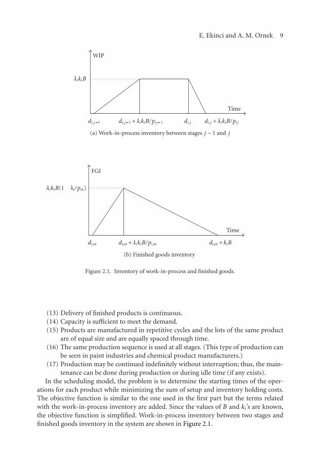
WIP
di, j + λikiB/pi jdi, jdi, j�1 di, j�1 + λikiB/pi j�1
λikiB
Time
(a) Work-in-process inventory between stages j− 1 and j
λikiB(1� λi/pm)
FGI
di,m + kiBdi,m di,m + λikiB/pi,m
Time
(b) Finished goods inventory
Figure 2.1. Inventory of work-in-process and finished goods.
(13) Delivery of finished products is continuous.(14) Capacity is sufficient to meet the demand.(15) Products are manufactured in repetitive cycles and the lots of the same product
are of equal size and are equally spaced through time.(16) The same production sequence is used at all stages. (This type of production can
be seen in paint industries and chemical product manufacturers.)(17) Production may be continued indefinitely without interruption; thus, the main-
tenance can be done during production or during idle time (if any exists).In the scheduling model, the problem is to determine the starting times of the oper-
ations for each product while minimizing the sum of setup and inventory holding costs.The objective function is similar to the one used in the first part but the terms relatedwith the work-in-process inventory are added. Since the values of B and ki’s are known,the objective function is simplified. Work-in-process inventory between two stages andfinished goods inventory in the system are shown in Figure 2.1.

10 Journal of Applied Mathematics and Decision Sciences
Using Figure 2.1(a), average work-in-process inventory for product i between stagesj− 1 and j can be calculated as
1kiB
{λikiB
2λikiB
pi, j−1+ λikiB
(di j −di, j−1− λikiB
pi j−1
)+λikiB
2λikiB
pi j
}
= λi
(di j +
λikiB
2pi j−di, j−1− λikiB
2pi j−1
).
(2.19)
Thus, the total work-in-process inventory holding cost per unit time is
n∑
i=1
m∑
j=2
hi, j−1λi
(di j +
λikiB
2pi j−di, j−1− λikiB
2pi j−1
). (2.20)
The total finished product inventory holding cost per unit time is
n∑
i=1
hi1kiB
(λikiB
2
(1− λi
pim
)(dim + kiB−dim
))=
n∑
i=1
hiλi2
(1− λi
pim
)(kiB
), (2.21)
which is constant.Other than holding costs, the objective function will include the setup costs. The setup
cost for product i per unit time is Ai/(kiB). Therefore, the objective function of the modelcan be written as
n∑
i=1
Ai
kiB+
n∑
i=1
m∑
j=2
hi, j−1λi
(di j +
λikiB
2pi j−di, j−1− λikiB
2pi j−1
)+
n∑
i=1
hiλi2
(1− λi
pim
)(kiB
).
(2.22)
Objective function should be modified in order to eliminate the constant terms thatdo not include a decision variable. In the scheduling model, the decision variables are di j ,mijl, and ai jl. In part 1, the values of B and ki are determined using the lot-sizing model,so in the objective function, only the terms including di j will remain,
n∑
i=1
m∑
j=2
hi, j−1λi(di j −di, j−1
). (2.23)
Since no product can be processed before its completion at the previous stage, we addthe following constraint which guarantees the processing times at each stage (2.24):
di, j−1 +λikiB
pi, j−1≤ di j . (2.24)
Also, the production end time after the last stage m can be shown using fi,
di,m +λikiB
pi,m≤ fi. (2.25)
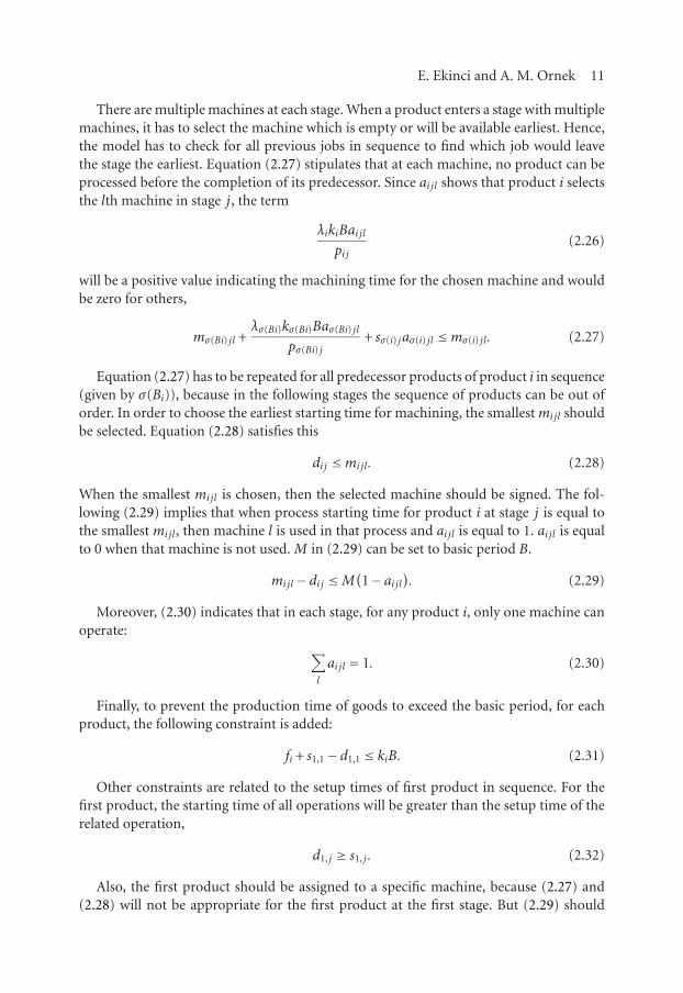
E. Ekinci and A. M. Ornek 11
There are multiple machines at each stage. When a product enters a stage with multiplemachines, it has to select the machine which is empty or will be available earliest. Hence,the model has to check for all previous jobs in sequence to find which job would leavethe stage the earliest. Equation (2.27) stipulates that at each machine, no product can beprocessed before the completion of its predecessor. Since ai jl shows that product i selectsthe lth machine in stage j, the term
λikiBai jlpi j
(2.26)
will be a positive value indicating the machining time for the chosen machine and wouldbe zero for others,
mσ(Bi) jl +λσ(Bi)kσ(Bi)Baσ(Bi) jl
pσ(Bi) j+ sσ(i) jaσ(i) jl ≤mσ(i) jl . (2.27)
Equation (2.27) has to be repeated for all predecessor products of product i in sequence(given by σ(Bi)), because in the following stages the sequence of products can be out oforder. In order to choose the earliest starting time for machining, the smallest mijl shouldbe selected. Equation (2.28) satisfies this
di j ≤mijl. (2.28)
When the smallest mijl is chosen, then the selected machine should be signed. The fol-lowing (2.29) implies that when process starting time for product i at stage j is equal tothe smallest mijl, then machine l is used in that process and ai jl is equal to 1. ai jl is equalto 0 when that machine is not used. M in (2.29) can be set to basic period B.
mijl −di j ≤M(1− ai jl
). (2.29)
Moreover, (2.30) indicates that in each stage, for any product i, only one machine canoperate:
∑
l
ai jl = 1. (2.30)
Finally, to prevent the production time of goods to exceed the basic period, for eachproduct, the following constraint is added:
fi + s1,1−d1,1 ≤ kiB. (2.31)
Other constraints are related to the setup times of first product in sequence. For thefirst product, the starting time of all operations will be greater than the setup time of therelated operation,
d1, j ≥ s1, j . (2.32)
Also, the first product should be assigned to a specific machine, because (2.27) and(2.28) will not be appropriate for the first product at the first stage. But (2.29) should
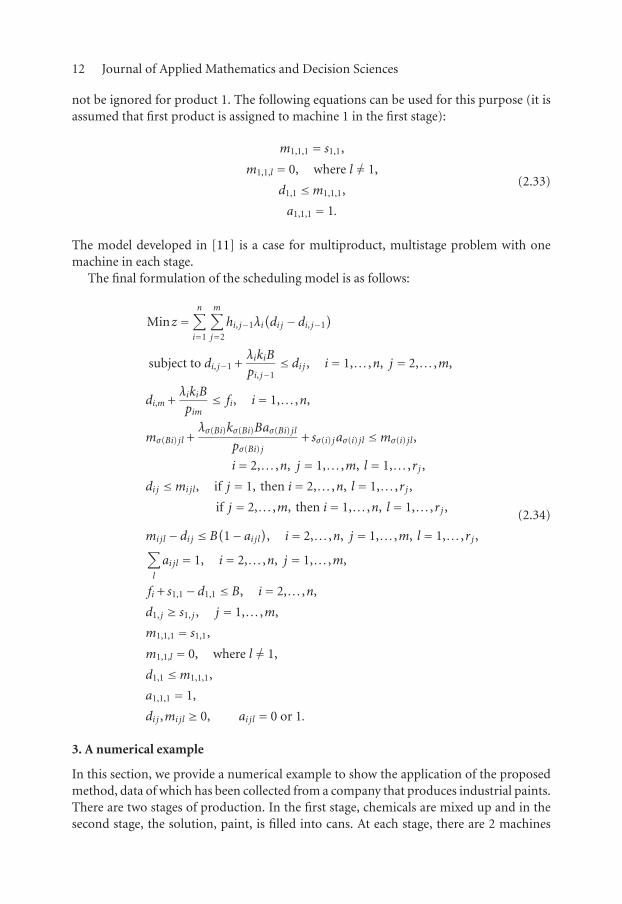
12 Journal of Applied Mathematics and Decision Sciences
not be ignored for product 1. The following equations can be used for this purpose (it isassumed that first product is assigned to machine 1 in the first stage):
m1,1,1 = s1,1,
m1,1,l = 0, where l �= 1,
d1,1 ≤m1,1,1,
a1,1,1 = 1.
(2.33)
The model developed in [11] is a case for multiproduct, multistage problem with onemachine in each stage.
The final formulation of the scheduling model is as follows:
Minz =n∑
i=1
m∑
j=2
hi, j−1λi(di j −di, j−1
)
subject to di, j−1 +λikiB
pi, j−1≤ di j , i= 1, . . . ,n, j = 2, . . . ,m,
di,m +λikiB
pim≤ fi, i= 1, . . . ,n,
mσ(Bi) jl +λσ(Bi)kσ(Bi)Baσ(Bi) jl
pσ(Bi) j+ sσ(i) jaσ(i) jl ≤mσ(i) jl,
i= 2, . . . ,n, j = 1, . . . ,m, l = 1, . . . ,r j ,
di j ≤mijl, if j = 1, then i= 2, . . . ,n, l = 1, . . . ,r j ,
if j = 2, . . . ,m, then i= 1, . . . ,n, l = 1, . . . ,r j ,
mijl −di j ≤ B(1− ai jl
), i= 2, . . . ,n, j = 1, . . . ,m, l = 1, . . . ,r j ,
∑
l
ai jl = 1, i= 2, . . . ,n, j = 1, . . . ,m,
fi + s1,1−d1,1 ≤ B, i= 2, . . . ,n,
d1, j ≥ s1, j , j = 1, . . . ,m,
m1,1,1 = s1,1,
m1,1,l = 0, where l �= 1,
d1,1 ≤m1,1,1,
a1,1,1 = 1,
di j ,mijl ≥ 0, ai jl = 0 or 1.
(2.34)
3. A numerical example
In this section, we provide a numerical example to show the application of the proposedmethod, data of which has been collected from a company that produces industrial paints.There are two stages of production. In the first stage, chemicals are mixed up and in thesecond stage, the solution, paint, is filled into cans. At each stage, there are 2 machines

E. Ekinci and A. M. Ornek 13
Table 3.1. Setup times and costs.
Stage 1 Stage 2Container size (kg) Setup time (min) Setup time (min) Setup cost ($)
800–1300 120 100 8
1300–3800 180 100 12
3800–7800 300 100 20
7800–15000 360 100 24
Table 3.2. Data for the product.
Productno.
Annualdemand(kg/year)
Production rate(kg/year) instage 1
Productionrate (kg/year)in stage 2
Productioncosts instage 1 ($/kg)
Totalproductioncosts ($/kg)
1 32000 2325000 2400000 2.83 3.11
2 138000 724000 750000 2.31 2.60
3 54500 766000 780000 2.31 2.66
4 27000 687000 700000 2.35 2.65
5 113000 546000 580000 2.30 2.59
Table 3.3. Total costs.
Basic period (days) Total cost ($) Basic period (days) Total cost ($)
1 5102.482 7 8966.13
2 5201.231 8 8966.13
3 6108.755 9 8966.13
4 4971.364 10 10187.89
5 7117.474 11 10960.28
6 7805.082 12 11142.78
performing the same job with the same production rate. Depending on the size of thecontainer used, the setup times and costs are given in Table 3.1.
Production of five different paints produced in the company is taken as an example,and the related data is given in Table 3.2.
Since the first stage of the production process is a bottleneck, we will use it as theproduction rate of the system to determine reorder intervals and lot sizes. To find theholding cost rate, we assume an interest rate of 30%.
Using (2.13) and (2.14), the upper and lower bounds for the basic period can be cal-culated. Since Trc = 0.000781 year = 0.28 day and Tcc = 0.033679 year = 12.3 days, it ismore convenient to use days from 1 to 12 as basic period candidates. For each basic pe-riod candidate, bounds for power-of-two multipliers are calculated using (2.8) and (2.9).After running the lot-size determination model, (2.10), the total costs obtained are givenin Table 3.3.
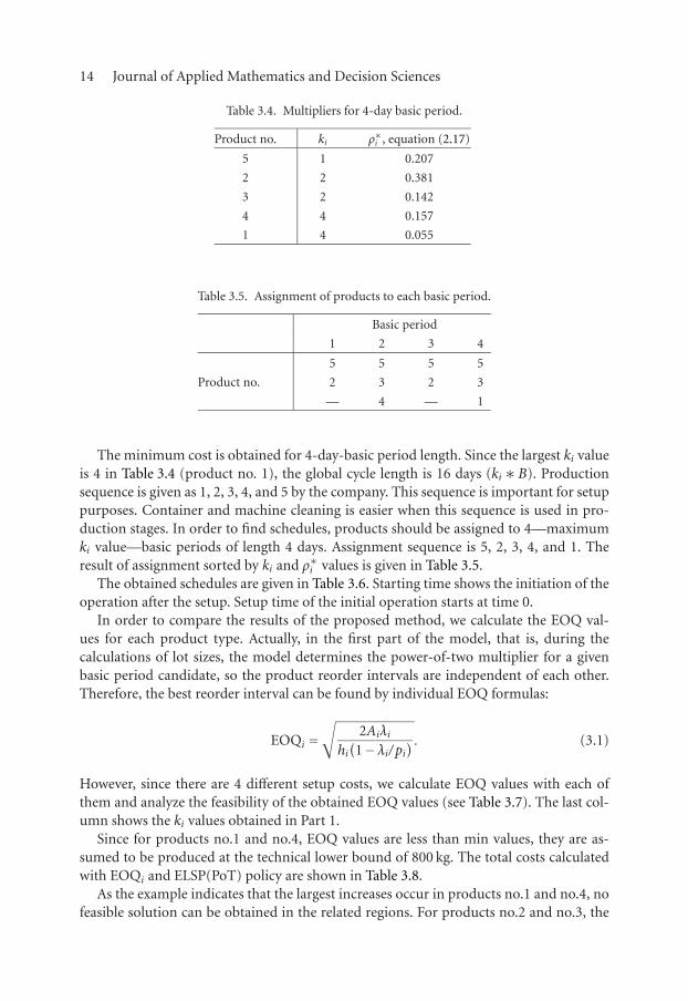
14 Journal of Applied Mathematics and Decision Sciences
Table 3.4. Multipliers for 4-day basic period.
Product no. ki ρ∗i , equation (2.17)
5 1 0.207
2 2 0.381
3 2 0.142
4 4 0.157
1 4 0.055
Table 3.5. Assignment of products to each basic period.
Basic period
1 2 3 4
Product no.
5 5 5 5
2 3 2 3
— 4 — 1
The minimum cost is obtained for 4-day-basic period length. Since the largest ki valueis 4 in Table 3.4 (product no. 1), the global cycle length is 16 days (ki ∗ B). Productionsequence is given as 1, 2, 3, 4, and 5 by the company. This sequence is important for setuppurposes. Container and machine cleaning is easier when this sequence is used in pro-duction stages. In order to find schedules, products should be assigned to 4—maximumki value—basic periods of length 4 days. Assignment sequence is 5, 2, 3, 4, and 1. Theresult of assignment sorted by ki and ρ∗i values is given in Table 3.5.
The obtained schedules are given in Table 3.6. Starting time shows the initiation of theoperation after the setup. Setup time of the initial operation starts at time 0.
In order to compare the results of the proposed method, we calculate the EOQ val-ues for each product type. Actually, in the first part of the model, that is, during thecalculations of lot sizes, the model determines the power-of-two multiplier for a givenbasic period candidate, so the product reorder intervals are independent of each other.Therefore, the best reorder interval can be found by individual EOQ formulas:
EOQi =√
2Aiλihi(1− λi/pi
) . (3.1)
However, since there are 4 different setup costs, we calculate EOQ values with each ofthem and analyze the feasibility of the obtained EOQ values (see Table 3.7). The last col-umn shows the ki values obtained in Part 1.
Since for products no.1 and no.4, EOQ values are less than min values, they are as-sumed to be produced at the technical lower bound of 800 kg. The total costs calculatedwith EOQi and ELSP(PoT) policy are shown in Table 3.8.
As the example indicates that the largest increases occur in products no.1 and no.4, nofeasible solution can be obtained in the related regions. For products no.2 and no.3, the
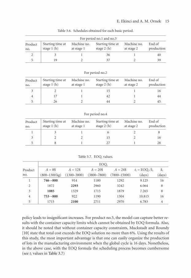
E. Ekinci and A. M. Ornek 15
Table 3.6. Schedules obtained for each basic period.
For period no.1 and no.3
Productno.
Starting time atstage 1 (h)
Machine no.at stage 1
Starting time atstage 2 (h)
Machine no.at stage 2
End ofproduction
2 3 1 36 1 40
5 19 2 37 2 39
For period no.2
Productno.
Starting time atstage 1 (h)
Machine no.at stage 1
Starting time atstage 2 (h)
Machine no.at stage 2
End ofproduction
3 2 1 15 1 16
4 17 1 42 1 44
5 26 2 44 2 45
For period no.4
Productno.
Starting time atstage 1 (h)
Machine no.at stage 1
Starting time atstage 2 (h)
Machine no.at stage 2
End ofproduction
1 3 1 6 2 8
3 2 2 15 2 16
5 8 1 27 1 28
Table 3.7. EOQi values.
EOQi
Productno.
A= 8$ A= 12$ A= 20$ A= 24$ ti = EOQi /λi ki
(800–1300 kg) (1300–3800) (3800–7800) (7800–15000) (days) (days)
1 746→800 914 1180 1292 9.125 16
2 1872 2293 2960 3242 6.064 8
3 1085 1329 1715 1879 7.265 8
4 753→800 922 1190 1304 10.815 16
5 1715 2100 2711 2970 6.783 4
policy leads to insignificant increases. For product no.5, the model can capture better re-sults with the container capacity limits which cannot be obtained by EOQ formula. Also,it should be noted that without container capacity constraints, Muckstadt and Roundy[10] state that total cost exceeds the EOQ solution no more than 6%. Using the results ofthis study, the most important advantage is that one can easily organize the productionof lots in the manufacturing environment when the global cycle is 16 days. Nonetheless,in the above case, with the EOQ formula the scheduling process becomes cumbersome(see ti values in Table 3.7)

16 Journal of Applied Mathematics and Decision Sciences
Table 3.8. Total cost and percentage change.
Product no. EOQi($) ELSP(PoT) ($) Change (%)
1 688 919 34
2 1445 1500 4
3 804 808 0
4 575 634 10
5 1291 1111 −14
Total 4803 4971 4
Finally, we note that the models were solved on P IV 3.2 MHz 512 Mb ram computerusing LINGO 8 software in a matter of seconds. Hence larger scale instances of the modelcan easily be solved.
4. Conclusions
In this paper, we propose a heuristic decomposition approach to model the problem ofdetermining realistic and easy-to-schedule lot sizes in a multiproduct, multistage, mul-timachine manufacturing environment using PoT policy. The approach is composed oftwo parts in order to find solutions to reorder interval determination (and consequentlylot sizing), and assignment and scheduling problems separately.
In the first part of the method, we develop a binary integer programming model to findoptimum reorder intervals which are power-of-two multiples of a basic period. The basicperiod length can be a day, a week, or a month to secure a realistic time period. As theoptimum reorder intervals are determined, we then calculate the optimum lot sizes foreach product. The basic contribution of the first model of the decomposition approach isthat we not only consider the technical upper and lower bounds of the production pro-cess, but also develop the formulation to accommodate process-dependent setup costs.To facilitate the solution of the problem, we assume the production system as a singleentity.
In the second part of the study, we first try to assign those lots to basic periods of theglobal cycle length (a cycle length in which production cycles of all products are com-pleted). Then a mixed integer programming model schedules the lots already assigned tobasic periods to multistages and multimachines at each stage.
Although the approach is designed for a specific flow-shop-type production, it couldbe easily modified to accommodate other types of production systems, for example, as-sembly systems.
Despite the problem is designed for deterministic demand, the results of lot sizingproblem are stable since they are based on reorder intervals rather than lot sizes. They
can be rescheduled again in case of small demand variations.
E. Ekinci and A. M. Ornek 17
Finally, in our opinion, the main advantage of the approach is that we find realisticand easy-to-apply reorder intervals. As seen in Tables 3.7 and 3.8, it is rather difficult toorder lots every 9.125 days for product no. 1, 6.064 days for product no. 2, and so forth,and on the overall, the cost increase is only 4%.
References
[1] W. B. Crowston, M. Wagner, and F. Williams, “Economic lot size determination in multi-stageassembly systems,” Management Science, vol. 19, pp. 517–527, 1973.
[2] P. A. Jensen and H. A. Khan, “Scheduling in a multistage production system with set-up andinventory costs,” AIIE Transactions, vol. 4, no. 2, pp. 126–133, 1972.
[3] B. A. Kalymon, “A decomposition algorithm for arborescence inventory systems,” OperationsResearch, vol. 20, pp. 860–874, 1972.
[4] A. M. Ornek and P. Collier, “The determination of in-process inventory and manufacturinglead time in multi-stage production systems,” International Journal of Operations & ProductionManagement, vol. 8, no. 1, pp. 74–80, 1988.
[5] A. M. Ornek and O. Cengiz, “Capacitated lot sizing with alternative routings and overtime de-cisions,” International Journal of Production Research, vol. 44, no. 24, pp. 5363–5389, 2006.
[6] L. B. Schwarz and L. Schrage, “Optimal and system myopic policies for multi-echelon produc-tion/inventory assembly systems,” Management Science, vol. 21, no. 11, pp. 1285–1294, 1975.
[7] A. Z. Szendrovits, “Manufacturing cycle time determination for a multi-stage economic pro-duction quantity model,” Management Science, vol. 22, no. 3, pp. 298–308, 1975.
[8] P. L. Jackson, W. L. Maxwell, and J. A. Muckstadt, “Determining optimal reorder intervals incapacitated production-distribution systems,” Management Science, vol. 34, no. 8, pp. 938–958,1988.
[9] W. L. Maxwell and J. A. Muckstadt, “Establishing consistent and realistic reorder intervals inproduction-distribution systems,” Operations Research, vol. 33, no. 6, pp. 1316–1341, 1985.
[10] J. A. Muckstadt and R. O. Roundy, “Analysis of multi-stage production systems,” in Logistics ofProduction and Inventory, S. Graves, A. H. G. Rinnooy Kan, and P. Zipkin, Eds., vol. 4 of Hand-book in Operations Research and Management Sci., pp. 59–131, North-Holland, Amsterdam, TheNetherlands, 1993.
[11] J. Ouenniche and F. F. Boctor, “The multi-product, economic lot-sizing problem in flow shops:the powers-of-two heuristic,” Computers & Operations Research, vol. 28, no. 12, pp. 1165–1182,2001.
[12] P. Jackson, W. Maxwell, and J. Muckstadt, “The joint replenishment problem with a powers-of-two restriction,” IIE Transactions, vol. 17, no. 1, pp. 25–32, 1985.
[13] R. Roundy, “98%-effective integer-ratio lot-sizing for one-warehouse multi-retailer systems,”Management Science, vol. 31, no. 11, pp. 1416–1430, 1985.
[14] J. A. Muckstadt and R. O. Roundy, “Multi-item, one-warehouse, multi-retailer distribution sys-tems,” Management Science, vol. 33, no. 12, pp. 1613–1621, 1987.
[15] D. Atkins, M. Queyranne, and D. Sun, “Lot sizing policies for finite production rate assemblysystems,” Operations Research, vol. 40, no. 1, pp. 126–141, 1992.
[16] D. Atkins and D. Sun, “98%-effective lot sizing for series inventory systems with backlogging,”Operations Research, vol. 43, no. 2, pp. 335–345, 1995.
[17] M. K. El-Najdawi, “A job-splitting heuristic for lot-size scheduling in multi-stage, multi-productproduction processes,” European Journal of Operational Research, vol. 75, no. 2, pp. 365–377,1994.
[18] M. K. El-Najdawi, “Multi-cyclic flow shop scheduling: an application in multi-stage, multi-product production processes,” International Journal of Production Research, vol. 35, no. 12, pp.3323–3332, 1997.
18 Journal of Applied Mathematics and Decision Sciences
[19] J. Ouenniche and F. F. Boctor, “The G-group heuristic to solve the multi-product, sequencing,lot sizing and scheduling problem in flow shops,” International Journal of Production Research,vol. 39, no. 1, pp. 81–98, 2001.
[20] J. Ouenniche and F. F. Boctor, “The two-group heuristic to solve the multi-product, economiclot sizing and scheduling problem in flow shops,” European Journal of Operational Research,vol. 129, no. 3, pp. 539–554, 2001.
[21] M.-J. Yao and S. E. Elmaghraby, “The economic lot scheduling problem under power-of-twopolicy,” Computers & Mathematics with Applications, vol. 41, no. 10-11, pp. 1379–1393, 2001.
[22] F.-C. Lee and M.-J. Yao, “A global optimum search algorithm for the joint replenishment prob-lem under power-of-two policy,” Computers & Operations Research, vol. 30, no. 9, pp. 1319–1333, 2003.
[23] J. Ouenniche, F. F. Boctor, and A. Martel, “The impact of sequencing decisions on multi-itemlot sizing and scheduling in flow shops,” International Journal of Production Research, vol. 37,no. 10, pp. 2253–2270, 1999.
Esra Ekinci: Industrial Engineering Depatment, Dokuz Eylul University, Bornova,35100 Izmir, TurkeyEmail address: [email protected]
Arslan M. Ornek: Industrial Engineering Depatment, Dokuz Eylul University, Bornova,35100 Izmir, TurkeyEmail address: [email protected]