Beyond the VisibleA handbook of best practice in

plant UV photobiology

edited byPedro J. Aphalo

withAndreas Albert Lars Olof Björn

Andy R. McLeod T. Matthew RobsonEva Rosenqvist

COST Action FA0906

Beyond the visible

A handbook of best practice in plant UV photobiology

COST action F0906 ‘UV4growth’

Beyond the visible

A handbook of best practice in plant UV photobiology

Edited byPedro J. Aphalo

with

Andreas Albert Lars Olof Björn Andy McLeod T. Matthew Robson Eva Rosenqvist

© COST office 2012No permission to reproduce or utilise the contents of this book by any means is necessary, other than in the case ofimages, diagrams or other material from other copyright holders. In such cases, permission of the copyright holders isrequired.This book may be cited as: COST Action FA0906 — Beyond the visible: A handbook of best practice in plant UVphotobiology.Neither the COST Office nor any person acting on its behalf is responsible for the use which might be made of theinformation contained in this publication. The COST Office is not responsible for the external websites referred to inthis publication.

ESF provides the COST office through an EC contract

COST is supported by the EU RTD framework programme

Full citation:Aphalo, P. J.; Albert, A.; Björn, L. O.; McLeod, A.; Robson, T. M.; Rosenqvist, E. (eds.) 2012. Beyond the visible: Ahandbook of best practice in plant UV photobiology. COST Action FA0906 UV4growth. Helsinki: University of Helsinki,Division of Plant Biology. ISBN 978-952-10-8362-4 (Paperback), 978-952-10-8363-1 (PDF). xxx + 176 pp.

First edition, first printing: November 2012.

Published by the University of Helsinki, Department of Biosciences, Division of Plant Biology, Helsinki, Finland.Paperback edition printed through CreateSpace Independent Publishing PlatformISBN-13: 978-952-10-8362-4 (Paperback)ISBN-13: 978-952-10-8363-1 (PDF)

Typeset with LATEX in Lucida Bright and Lucida Sans using the KOMA-Script book class.Most data plots were produced with the R System for statistics with package ggplot2. Flowcharts drawn with yEd.Edited with WinEdt.

COST

COST —the acronym for European Cooperation in Sci-ence and Technology— is the oldest and widest Europeanintergovernmental network for cooperation in research.Established by the Ministerial Conference in November1971, COST is presently used by the scientific communit-ies of 36 European countries to cooperate in commonresearch projects supported by national funds.

The funds provided by COST —less than 1% of the totalvalue of the projects— support the COST cooperationnetworks (COST Actions) through which, with EUR 30 mil-lion per year, more than 30 000 European scientists areinvolved in research having a total value which exceedsEUR 2 billion per year. This is the financial worth of theEuropean added value which COST achieves.

A “bottom up approach” (the initiative of launching aCOST Action comes from the European scientists them-selves), “à la carte participation” (only countries inter-ested in the Action participate), “equality of access” (par-ticipation is open also to the scientific communities ofcountries not belonging to the European Union) and “flex-ible structure” (easy implementation and light manage-

ment of the research initiatives) are the main character-istics of COST.

As precursor of advanced multidisciplinary researchCOST has a very important role for the realisation ofthe European Research Area (ERA) anticipating and com-plementing the activities of the Framework Programmes,constituting a “bridge” towards the scientific communit-ies of emerging countries, increasing the mobility of re-searchers across Europe and fostering the establishmentof “Networks of Excellence” in many key scientific do-mains such as: Biomedicine and Molecular Biosciences;Food and Agriculture; Forests, their Products and Ser-vices; Materials, Physical and Nanosciences; Chemistryand Molecular Sciences and Technologies; Earth SystemScience and Environmental Management; Information andCommunication Technologies; Transport and Urban De-velopment; Individuals, Societies, Cultures and Health.It covers basic and more applied research and also ad-dresses issues of pre-normative nature or of societalimportance.

Web: http://www.cost.eu

v

Foreword

The discovery of the thinning of the stratospheric ozonelayer in the 1980s, and subsequent measurements of in-creased penetration of UV-B in the biosphere, triggeredextensive research in the photobiology of UV radiation.Initially, the central aim of research was to assess the im-pacts of increases in UV-B radiation on various organismsand ecosystems. More recently, the question how currentlevels of UV affect life-processes has become increasinglyimportant. Several decades of UV research have now ledto a much more detailed understanding of the, ratherbroad, impacts of UV on plant, microbial and animallife. Emphasis has gradually shifted away from a stress-dominated view (sunburn in humans and farm animals;macroscopic damage and growth inhibition in plants) toa more balanced vision which also includes many subtle,regulatory UV-effects. For example, many vertebratesgather information from UV wavelengths which they canperceive due to their tetrachromatic colour vision. Birdsappear to use UV wavelengths for orientation and nav-igation, while both birds and lizards have UV-reflectivefeatures that play a role in mate choice. Several rodents,including house mice, can perceive UV-light, while theirurine fluoresces under UV, consequently it has been sug-gested that these rodents may use UV cues for intraspe-cific signalling. Another mammal able to perceive UVwavelengths is the reindeer, which is thought to obtaininformation from differential UV reflections of Arctic ve-getation. Plants are not to be left out of this wonderful(for human’s invisible) UV world: One of the most im-portant discoveries in plant UV-B biology has been theidentification of a specific UV-B photoreceptor. Thus,plants also “see” UV-B and the so-called UVR8 photore-ceptor has, among others, been implicated in controllingthe development of plant morphology in UV-B exposedplants.

Notwithstanding these fascinating advances in UV bio-logy, the development of an overarching vision on thebiological role of UV wavelengths remains elusive. Thisis partly due to the use of a rather diverse range of UV-exposure and quantification technologies, in combination

with action spectra that are not always appropriate. Con-sequent variations in applied dose and spectrum haveaffected the reproducibility of research across differentlaboratories, and have sometimes necessitated extensivetrialling to repeat published data. A related issue con-cerns the extrapolation of laboratory data, generated in-doors using artificial UV sources and/or filtration set-ups,to more ecologically relevant scenarios. There is no doubtthat indoor experimentation, under rather unnatural con-ditions, has generated conceptually critical informationabout UV-perception, and UV-mediated signalling andgene transcription. Nevertheless, one important lessonlearnt from three decades of plant UV-research is thattime spent on devising an experimental set-up that is as“environmentally sound” as feasible, is time well spent(climate change biologists, please take note!).

This book entitled “Beyond the visible: A handbook ofbest practice in plant UV photobiology” is an importantcontribution towards such sound experimental design,promoting both “good practice” in UV-B manipulation,as well as “standardisation” of methodologies. Writingan authoritative book that will steer experimental ap-proaches over the coming years, can not easily be done byan individual, but rather requires the concerted effort ofa team of expert scientists. I commend the main author,Dr. Pedro J. Aphalo, who assembled a team of leading UV-scientists, and I congratulate all the authors on a text thatis both accessible as well as in-depth. I also gratefullyacknowledge the financial support of COST (EuropeanCooperation in Science and Technology), who throughCOST Action UV4Growth (FA0906) made it possible forthe main authors to meet, coordinate and write. Thisis surely an excellent example of a concerted, European-wide activity that will boost the plant UV-B research fieldin Europe and beyond, for years to come.

Happy reading,

Cork, August 2012 Dr. Marcel A. K. JansenChair, COST Action UV4Growth

vii

Contents

COST v

Foreword vii

Contributors xxi

List of abbreviations and symbols xxiii

Preface xxvii

Acknowledgements xxix

1 Introduction 11.1 Research on plant responses to ultraviolet radiation . . . . . . . . . . . . . . . . . . . . . . . . . . . . . . . . 11.2 The principles of photochemistry . . . . . . . . . . . . . . . . . . . . . . . . . . . . . . . . . . . . . . . . . . . 21.3 Physical properties of ultraviolet and visible radiation . . . . . . . . . . . . . . . . . . . . . . . . . . . . . . 21.4 UV in solar radiation . . . . . . . . . . . . . . . . . . . . . . . . . . . . . . . . . . . . . . . . . . . . . . . . . . . 81.5 UV radiation within plant canopies . . . . . . . . . . . . . . . . . . . . . . . . . . . . . . . . . . . . . . . . . . 111.6 UV radiation in aquatic environments . . . . . . . . . . . . . . . . . . . . . . . . . . . . . . . . . . . . . . . . . 15

1.6.1 Refraction . . . . . . . . . . . . . . . . . . . . . . . . . . . . . . . . . . . . . . . . . . . . . . . . . . . . . . 151.6.2 Absorption and scattering by pure water . . . . . . . . . . . . . . . . . . . . . . . . . . . . . . . . . . . 161.6.3 Absorption and scattering by water constituents . . . . . . . . . . . . . . . . . . . . . . . . . . . . . . 161.6.4 Results and effects . . . . . . . . . . . . . . . . . . . . . . . . . . . . . . . . . . . . . . . . . . . . . . . . 181.6.5 Modelling of underwater radiation . . . . . . . . . . . . . . . . . . . . . . . . . . . . . . . . . . . . . . . 19

1.7 UV radiation within plant leaves . . . . . . . . . . . . . . . . . . . . . . . . . . . . . . . . . . . . . . . . . . . . 211.7.1 Fibre-optic measurements . . . . . . . . . . . . . . . . . . . . . . . . . . . . . . . . . . . . . . . . . . . . 211.7.2 UV-induced chlorophyll fluorescence . . . . . . . . . . . . . . . . . . . . . . . . . . . . . . . . . . . . . 211.7.3 Factors affecting internal UV levels . . . . . . . . . . . . . . . . . . . . . . . . . . . . . . . . . . . . . . 21

1.8 Action and response spectra . . . . . . . . . . . . . . . . . . . . . . . . . . . . . . . . . . . . . . . . . . . . . . 211.8.1 Constructing a monochromatic action spectrum . . . . . . . . . . . . . . . . . . . . . . . . . . . . . . 231.8.2 Constructing a polychromatic action spectrum . . . . . . . . . . . . . . . . . . . . . . . . . . . . . . . 241.8.3 Action spectra in the field . . . . . . . . . . . . . . . . . . . . . . . . . . . . . . . . . . . . . . . . . . . . 27

1.9 Further reading . . . . . . . . . . . . . . . . . . . . . . . . . . . . . . . . . . . . . . . . . . . . . . . . . . . . . . . 271.10 Appendix: Calculation of polychromatic action spectra with Excel (using add-in “Solver”) . . . . . . . . 27

2 Manipulating UV radiation 352.1 Safety considerations . . . . . . . . . . . . . . . . . . . . . . . . . . . . . . . . . . . . . . . . . . . . . . . . . . . 35

2.1.1 Risks related to sunlight exposure . . . . . . . . . . . . . . . . . . . . . . . . . . . . . . . . . . . . . . . 352.1.2 Risks related to the use of UV lamps . . . . . . . . . . . . . . . . . . . . . . . . . . . . . . . . . . . . . 352.1.3 Risks related to electrical power . . . . . . . . . . . . . . . . . . . . . . . . . . . . . . . . . . . . . . . . 362.1.4 Safety regulations and recommendations . . . . . . . . . . . . . . . . . . . . . . . . . . . . . . . . . . 36

2.2 Artificial sources of UV radiation . . . . . . . . . . . . . . . . . . . . . . . . . . . . . . . . . . . . . . . . . . . . 362.2.1 Lamps . . . . . . . . . . . . . . . . . . . . . . . . . . . . . . . . . . . . . . . . . . . . . . . . . . . . . . . . 362.2.2 Deuterium lamps . . . . . . . . . . . . . . . . . . . . . . . . . . . . . . . . . . . . . . . . . . . . . . . . . 422.2.3 LEDs . . . . . . . . . . . . . . . . . . . . . . . . . . . . . . . . . . . . . . . . . . . . . . . . . . . . . . . . . 422.2.4 Spectrographs . . . . . . . . . . . . . . . . . . . . . . . . . . . . . . . . . . . . . . . . . . . . . . . . . . . 442.2.5 Lasers . . . . . . . . . . . . . . . . . . . . . . . . . . . . . . . . . . . . . . . . . . . . . . . . . . . . . . . . 452.2.6 Modulated UV-B supplementation systems . . . . . . . . . . . . . . . . . . . . . . . . . . . . . . . . . 48

ix

Contents

2.2.7 Exposure chambers and sun simulators . . . . . . . . . . . . . . . . . . . . . . . . . . . . . . . . . . . 482.3 Filters . . . . . . . . . . . . . . . . . . . . . . . . . . . . . . . . . . . . . . . . . . . . . . . . . . . . . . . . . . . . . 52

2.3.1 Optical properties of filters . . . . . . . . . . . . . . . . . . . . . . . . . . . . . . . . . . . . . . . . . . . 522.3.2 Manipulating UV radiation in sunlight . . . . . . . . . . . . . . . . . . . . . . . . . . . . . . . . . . . . 542.3.3 Measuring the spectral transmittance of filters . . . . . . . . . . . . . . . . . . . . . . . . . . . . . . . 62

2.4 Manipulating UV-B in the aquatic environment . . . . . . . . . . . . . . . . . . . . . . . . . . . . . . . . . . . 622.4.1 Incubations in the field . . . . . . . . . . . . . . . . . . . . . . . . . . . . . . . . . . . . . . . . . . . . . . 622.4.2 Incubation under artificial lamps . . . . . . . . . . . . . . . . . . . . . . . . . . . . . . . . . . . . . . . . 63

2.5 Suitable treatments and controls . . . . . . . . . . . . . . . . . . . . . . . . . . . . . . . . . . . . . . . . . . . . 632.6 Recommendations . . . . . . . . . . . . . . . . . . . . . . . . . . . . . . . . . . . . . . . . . . . . . . . . . . . . . 64

2.6.1 Recommendations for outdoor experiments . . . . . . . . . . . . . . . . . . . . . . . . . . . . . . . . . 642.6.2 Recommendations for experiments in greenhouses and controlled environments . . . . . . . . . 67

2.7 Further reading . . . . . . . . . . . . . . . . . . . . . . . . . . . . . . . . . . . . . . . . . . . . . . . . . . . . . . . 672.8 Appendix: Radiation field calculations . . . . . . . . . . . . . . . . . . . . . . . . . . . . . . . . . . . . . . . . 672.9 Appendix: Suppliers of light sources and filters . . . . . . . . . . . . . . . . . . . . . . . . . . . . . . . . . . 68

3 Quantifying UV radiation 713.1 Basic concepts and terminology . . . . . . . . . . . . . . . . . . . . . . . . . . . . . . . . . . . . . . . . . . . . 71

3.1.1 Introduction to UV and visible radiation . . . . . . . . . . . . . . . . . . . . . . . . . . . . . . . . . . . 713.1.2 Direction . . . . . . . . . . . . . . . . . . . . . . . . . . . . . . . . . . . . . . . . . . . . . . . . . . . . . . 713.1.3 Spectral irradiance . . . . . . . . . . . . . . . . . . . . . . . . . . . . . . . . . . . . . . . . . . . . . . . . 723.1.4 Wavelength . . . . . . . . . . . . . . . . . . . . . . . . . . . . . . . . . . . . . . . . . . . . . . . . . . . . . 723.1.5 Units used for photons and energy . . . . . . . . . . . . . . . . . . . . . . . . . . . . . . . . . . . . . . 733.1.6 Ratios of UV and visible radiation . . . . . . . . . . . . . . . . . . . . . . . . . . . . . . . . . . . . . . . 733.1.7 A practical example . . . . . . . . . . . . . . . . . . . . . . . . . . . . . . . . . . . . . . . . . . . . . . . . 743.1.8 Measuring fluence rate and radiance . . . . . . . . . . . . . . . . . . . . . . . . . . . . . . . . . . . . . 743.1.9 Sensor output . . . . . . . . . . . . . . . . . . . . . . . . . . . . . . . . . . . . . . . . . . . . . . . . . . . 743.1.10 Calibration . . . . . . . . . . . . . . . . . . . . . . . . . . . . . . . . . . . . . . . . . . . . . . . . . . . . . 743.1.11 Further reading . . . . . . . . . . . . . . . . . . . . . . . . . . . . . . . . . . . . . . . . . . . . . . . . . . 76

3.2 Actinometry . . . . . . . . . . . . . . . . . . . . . . . . . . . . . . . . . . . . . . . . . . . . . . . . . . . . . . . . . 763.3 Dosimeters . . . . . . . . . . . . . . . . . . . . . . . . . . . . . . . . . . . . . . . . . . . . . . . . . . . . . . . . . 783.4 Thermopiles . . . . . . . . . . . . . . . . . . . . . . . . . . . . . . . . . . . . . . . . . . . . . . . . . . . . . . . . . 793.5 Broadband instruments . . . . . . . . . . . . . . . . . . . . . . . . . . . . . . . . . . . . . . . . . . . . . . . . . . 79

3.5.1 Principle of operation . . . . . . . . . . . . . . . . . . . . . . . . . . . . . . . . . . . . . . . . . . . . . . . 803.5.2 Some commonly used terrestrial instruments . . . . . . . . . . . . . . . . . . . . . . . . . . . . . . . . 823.5.3 Spectral and angular (cosine) response . . . . . . . . . . . . . . . . . . . . . . . . . . . . . . . . . . . . 823.5.4 Calibration and intercomparison . . . . . . . . . . . . . . . . . . . . . . . . . . . . . . . . . . . . . . . . 833.5.5 UV radiation monitoring in growth chambers, greenhouses and phytotrons . . . . . . . . . . . . . 84

3.6 Multi-channel filter instruments . . . . . . . . . . . . . . . . . . . . . . . . . . . . . . . . . . . . . . . . . . . . 843.7 Spectroradiometers . . . . . . . . . . . . . . . . . . . . . . . . . . . . . . . . . . . . . . . . . . . . . . . . . . . . 85

3.7.1 Scanning spectroradiometers . . . . . . . . . . . . . . . . . . . . . . . . . . . . . . . . . . . . . . . . . . 853.7.2 Array detector spectroradiometers . . . . . . . . . . . . . . . . . . . . . . . . . . . . . . . . . . . . . . 88

3.8 Underwater sensors and profiling . . . . . . . . . . . . . . . . . . . . . . . . . . . . . . . . . . . . . . . . . . . 943.8.1 Measuring underwater UV radiation . . . . . . . . . . . . . . . . . . . . . . . . . . . . . . . . . . . . . . 943.8.2 Profiling . . . . . . . . . . . . . . . . . . . . . . . . . . . . . . . . . . . . . . . . . . . . . . . . . . . . . . . 953.8.3 Underwater radiometers . . . . . . . . . . . . . . . . . . . . . . . . . . . . . . . . . . . . . . . . . . . . . 95

3.9 Modelling . . . . . . . . . . . . . . . . . . . . . . . . . . . . . . . . . . . . . . . . . . . . . . . . . . . . . . . . . . 973.10 BSWFs and effective UV doses . . . . . . . . . . . . . . . . . . . . . . . . . . . . . . . . . . . . . . . . . . . . . . 99

3.10.1 Weighting scales . . . . . . . . . . . . . . . . . . . . . . . . . . . . . . . . . . . . . . . . . . . . . . . . . . 1013.10.2 Comparing lamps and solar radiation . . . . . . . . . . . . . . . . . . . . . . . . . . . . . . . . . . . . . 1023.10.3 Effective doses, enhancement errors and UV-B supplementation . . . . . . . . . . . . . . . . . . . . 102

3.11 Effective UV doses outdoors . . . . . . . . . . . . . . . . . . . . . . . . . . . . . . . . . . . . . . . . . . . . . . . 1053.12 Effective UV doses in controlled environments . . . . . . . . . . . . . . . . . . . . . . . . . . . . . . . . . . . 1053.13 An accuracy ranking of quantification methods . . . . . . . . . . . . . . . . . . . . . . . . . . . . . . . . . . . 107

x

Contents

3.14 Sanity checks for data and calculations . . . . . . . . . . . . . . . . . . . . . . . . . . . . . . . . . . . . . . . . 1073.15 Recommendations . . . . . . . . . . . . . . . . . . . . . . . . . . . . . . . . . . . . . . . . . . . . . . . . . . . . . 1073.16 Further reading . . . . . . . . . . . . . . . . . . . . . . . . . . . . . . . . . . . . . . . . . . . . . . . . . . . . . . . 110

3.16.1 UV climatology and modelling . . . . . . . . . . . . . . . . . . . . . . . . . . . . . . . . . . . . . . . . . 1103.16.2 Instrumentation and UV measurement validation . . . . . . . . . . . . . . . . . . . . . . . . . . . . . 1103.16.3 Books . . . . . . . . . . . . . . . . . . . . . . . . . . . . . . . . . . . . . . . . . . . . . . . . . . . . . . . . . 111

3.17 Appendix: Formulations for action spectra used as BSWFs . . . . . . . . . . . . . . . . . . . . . . . . . . . . 1113.18 Appendix: Calculation of effective doses with Excel . . . . . . . . . . . . . . . . . . . . . . . . . . . . . . . . 1123.19 Appendix: Calculation of effective doses with R . . . . . . . . . . . . . . . . . . . . . . . . . . . . . . . . . . 113

3.19.1 Introduction . . . . . . . . . . . . . . . . . . . . . . . . . . . . . . . . . . . . . . . . . . . . . . . . . . . . 1133.19.2 Calculating doses . . . . . . . . . . . . . . . . . . . . . . . . . . . . . . . . . . . . . . . . . . . . . . . . . 1133.19.3 Calculating an action spectrum at given wavelengths . . . . . . . . . . . . . . . . . . . . . . . . . . . 1153.19.4 Calculating photon ratios . . . . . . . . . . . . . . . . . . . . . . . . . . . . . . . . . . . . . . . . . . . . 1163.19.5 Documentation . . . . . . . . . . . . . . . . . . . . . . . . . . . . . . . . . . . . . . . . . . . . . . . . . . . 116

3.20 Appendix: Suppliers of instruments . . . . . . . . . . . . . . . . . . . . . . . . . . . . . . . . . . . . . . . . . . 116

4 Plant growing conditions 1194.1 Introduction . . . . . . . . . . . . . . . . . . . . . . . . . . . . . . . . . . . . . . . . . . . . . . . . . . . . . . . . . 1194.2 Greenhouses . . . . . . . . . . . . . . . . . . . . . . . . . . . . . . . . . . . . . . . . . . . . . . . . . . . . . . . . 119

4.2.1 Temperature . . . . . . . . . . . . . . . . . . . . . . . . . . . . . . . . . . . . . . . . . . . . . . . . . . . . 1194.2.2 Light . . . . . . . . . . . . . . . . . . . . . . . . . . . . . . . . . . . . . . . . . . . . . . . . . . . . . . . . . 1204.2.3 Air humidity . . . . . . . . . . . . . . . . . . . . . . . . . . . . . . . . . . . . . . . . . . . . . . . . . . . . 1244.2.4 Elevated carbon dioxide concentration . . . . . . . . . . . . . . . . . . . . . . . . . . . . . . . . . . . . 1264.2.5 Growth substrates, irrigation and fertilization . . . . . . . . . . . . . . . . . . . . . . . . . . . . . . . 1264.2.6 Data logging of microclimatic variables . . . . . . . . . . . . . . . . . . . . . . . . . . . . . . . . . . . . 127

4.3 Open top chambers and FACE . . . . . . . . . . . . . . . . . . . . . . . . . . . . . . . . . . . . . . . . . . . . . . 1274.4 Controlled environments . . . . . . . . . . . . . . . . . . . . . . . . . . . . . . . . . . . . . . . . . . . . . . . . . 1274.5 Material issues in greenhouses and controlled environments . . . . . . . . . . . . . . . . . . . . . . . . . . 1294.6 Gas-exchange cuvettes and chambers . . . . . . . . . . . . . . . . . . . . . . . . . . . . . . . . . . . . . . . . . 1314.7 Plants in the field . . . . . . . . . . . . . . . . . . . . . . . . . . . . . . . . . . . . . . . . . . . . . . . . . . . . . 1314.8 Cultivation of aquatic plants . . . . . . . . . . . . . . . . . . . . . . . . . . . . . . . . . . . . . . . . . . . . . . 1314.9 Recommendations . . . . . . . . . . . . . . . . . . . . . . . . . . . . . . . . . . . . . . . . . . . . . . . . . . . . . 1364.10 Further reading . . . . . . . . . . . . . . . . . . . . . . . . . . . . . . . . . . . . . . . . . . . . . . . . . . . . . . . 138

5 Statistical design of UV experiments 1395.1 Tests of hypotheses and model fitting . . . . . . . . . . . . . . . . . . . . . . . . . . . . . . . . . . . . . . . . 1395.2 Planning of experiments . . . . . . . . . . . . . . . . . . . . . . . . . . . . . . . . . . . . . . . . . . . . . . . . . 1405.3 Definitions . . . . . . . . . . . . . . . . . . . . . . . . . . . . . . . . . . . . . . . . . . . . . . . . . . . . . . . . . . 1405.4 Experimental design . . . . . . . . . . . . . . . . . . . . . . . . . . . . . . . . . . . . . . . . . . . . . . . . . . . . 1405.5 Requirements for a good experiment . . . . . . . . . . . . . . . . . . . . . . . . . . . . . . . . . . . . . . . . . 1425.6 The principles of experimental design . . . . . . . . . . . . . . . . . . . . . . . . . . . . . . . . . . . . . . . . 142

5.6.1 Replication . . . . . . . . . . . . . . . . . . . . . . . . . . . . . . . . . . . . . . . . . . . . . . . . . . . . . 1425.6.2 Randomization . . . . . . . . . . . . . . . . . . . . . . . . . . . . . . . . . . . . . . . . . . . . . . . . . . . 1425.6.3 Blocks and covariates . . . . . . . . . . . . . . . . . . . . . . . . . . . . . . . . . . . . . . . . . . . . . . . 142

5.7 Experimental units and subsamples . . . . . . . . . . . . . . . . . . . . . . . . . . . . . . . . . . . . . . . . . . 1435.8 Pseudoreplication . . . . . . . . . . . . . . . . . . . . . . . . . . . . . . . . . . . . . . . . . . . . . . . . . . . . . 1435.9 Range of validity . . . . . . . . . . . . . . . . . . . . . . . . . . . . . . . . . . . . . . . . . . . . . . . . . . . . . . 146

5.9.1 Factorial experiments . . . . . . . . . . . . . . . . . . . . . . . . . . . . . . . . . . . . . . . . . . . . . . . 1485.10 When not to make multiple comparisons . . . . . . . . . . . . . . . . . . . . . . . . . . . . . . . . . . . . . . . 148

5.10.1 Dose response curves . . . . . . . . . . . . . . . . . . . . . . . . . . . . . . . . . . . . . . . . . . . . . . . 1485.10.2 Factorial experiments . . . . . . . . . . . . . . . . . . . . . . . . . . . . . . . . . . . . . . . . . . . . . . . 148

5.11 Presenting data in figures . . . . . . . . . . . . . . . . . . . . . . . . . . . . . . . . . . . . . . . . . . . . . . . . 1485.12 Recommendations . . . . . . . . . . . . . . . . . . . . . . . . . . . . . . . . . . . . . . . . . . . . . . . . . . . . . 1495.13 Further reading . . . . . . . . . . . . . . . . . . . . . . . . . . . . . . . . . . . . . . . . . . . . . . . . . . . . . . . 150

xi

Contents

Bibliography 151

Glossary 169

Index 171

xii

List of Tables

1.1 Regions of the electromagnetic radiation associated with colours . . . . . . . . . . . . . . . . . . . . . . . . . 31.2 Physical quantities of light. . . . . . . . . . . . . . . . . . . . . . . . . . . . . . . . . . . . . . . . . . . . . . . . . . 51.3 Distribution of the solar constant in different wavelength intervals . . . . . . . . . . . . . . . . . . . . . . . . 101.4 Action spectra . . . . . . . . . . . . . . . . . . . . . . . . . . . . . . . . . . . . . . . . . . . . . . . . . . . . . . . . . 251.5 PAR and UV radiation under coloured glass filter WG305 . . . . . . . . . . . . . . . . . . . . . . . . . . . . . . 28

2.1 Typical irradiance data from sun simulators . . . . . . . . . . . . . . . . . . . . . . . . . . . . . . . . . . . . . . 54

3.1 Quantum yield and the fraction of radiation absorbed by ferrioxalate . . . . . . . . . . . . . . . . . . . . . . 783.2 Broadband sensor errors . . . . . . . . . . . . . . . . . . . . . . . . . . . . . . . . . . . . . . . . . . . . . . . . . . 853.3 Simplified properties of methods for modelling of surface UV radiation . . . . . . . . . . . . . . . . . . . . . 983.4 Effective UV-B irradiances . . . . . . . . . . . . . . . . . . . . . . . . . . . . . . . . . . . . . . . . . . . . . . . . . . 1033.5 Shading compensation errors . . . . . . . . . . . . . . . . . . . . . . . . . . . . . . . . . . . . . . . . . . . . . . . 1033.6 Seasonal and latitudinal variation in effective UV doses . . . . . . . . . . . . . . . . . . . . . . . . . . . . . . . 1073.7 UV-quantification methods compared . . . . . . . . . . . . . . . . . . . . . . . . . . . . . . . . . . . . . . . . . . 1083.8 Typical irradiance values . . . . . . . . . . . . . . . . . . . . . . . . . . . . . . . . . . . . . . . . . . . . . . . . . . 1093.9 Functions in R package UVcalc: effective irradiances and doses . . . . . . . . . . . . . . . . . . . . . . . . . . 1163.10 Functions in R package UVcalc: action spectra . . . . . . . . . . . . . . . . . . . . . . . . . . . . . . . . . . . . . 1163.11 Functions in R package UVcalc: photon ratios . . . . . . . . . . . . . . . . . . . . . . . . . . . . . . . . . . . . . 117

4.1 Guidelines for controlled environments and greenhouses . . . . . . . . . . . . . . . . . . . . . . . . . . . . . . 1284.2 Describing controlled environments and greenhouses . . . . . . . . . . . . . . . . . . . . . . . . . . . . . . . . 130

xiii

List of Figures

1.1 Definition of the solid angles and areas in space . . . . . . . . . . . . . . . . . . . . . . . . . . . . . . . . . . . . 31.2 Path of the radiance in a thin layer. . . . . . . . . . . . . . . . . . . . . . . . . . . . . . . . . . . . . . . . . . . . . 51.3 Solar position . . . . . . . . . . . . . . . . . . . . . . . . . . . . . . . . . . . . . . . . . . . . . . . . . . . . . . . . . 91.4 Extraterrestrial solar spectrum . . . . . . . . . . . . . . . . . . . . . . . . . . . . . . . . . . . . . . . . . . . . . . . 101.5 Sky photos . . . . . . . . . . . . . . . . . . . . . . . . . . . . . . . . . . . . . . . . . . . . . . . . . . . . . . . . . . . 111.6 Diffuse component in solar UV . . . . . . . . . . . . . . . . . . . . . . . . . . . . . . . . . . . . . . . . . . . . . . . 121.7 The solar spectrum through half a day . . . . . . . . . . . . . . . . . . . . . . . . . . . . . . . . . . . . . . . . . . 121.8 The solar UV spectrum at noon . . . . . . . . . . . . . . . . . . . . . . . . . . . . . . . . . . . . . . . . . . . . . . 131.9 The solar UV spectrum through half a day . . . . . . . . . . . . . . . . . . . . . . . . . . . . . . . . . . . . . . . 131.10 UV-B and PAR . . . . . . . . . . . . . . . . . . . . . . . . . . . . . . . . . . . . . . . . . . . . . . . . . . . . . . . . . 141.11 Seasonal variation in UV-B radiation . . . . . . . . . . . . . . . . . . . . . . . . . . . . . . . . . . . . . . . . . . . 141.12 Latitudinal variation in UV-B radiation . . . . . . . . . . . . . . . . . . . . . . . . . . . . . . . . . . . . . . . . . . 151.13 Absorption and scattering of pure water . . . . . . . . . . . . . . . . . . . . . . . . . . . . . . . . . . . . . . . . 171.14 Specific absorption of chlorophyll . . . . . . . . . . . . . . . . . . . . . . . . . . . . . . . . . . . . . . . . . . . . . 191.15 Optical classification of marine waters . . . . . . . . . . . . . . . . . . . . . . . . . . . . . . . . . . . . . . . . . . 201.16 Underwater light climate . . . . . . . . . . . . . . . . . . . . . . . . . . . . . . . . . . . . . . . . . . . . . . . . . . 221.17 Chlorophyll fluorescence and UV radiation penetration into leaves . . . . . . . . . . . . . . . . . . . . . . . . 231.18 Constructing an action spectrum . . . . . . . . . . . . . . . . . . . . . . . . . . . . . . . . . . . . . . . . . . . . . 241.19 Action spectra . . . . . . . . . . . . . . . . . . . . . . . . . . . . . . . . . . . . . . . . . . . . . . . . . . . . . . . . . 251.20 Spectra of the different UV scenarios used in an experiment . . . . . . . . . . . . . . . . . . . . . . . . . . . . 261.21 Special cuvette covered by five types of coloured glass filter . . . . . . . . . . . . . . . . . . . . . . . . . . . . 281.22 Excel sheet for estimating polychromatic action spectra including input data of leaves . . . . . . . . . . . . 291.23 Excel sheet for estimating polychromatic action spectra including light level variation . . . . . . . . . . . . 301.24 Excel sheet for estimating polychromatic action spectra including calculation of biological effective dose

function . . . . . . . . . . . . . . . . . . . . . . . . . . . . . . . . . . . . . . . . . . . . . . . . . . . . . . . . . . . . . 311.25 Excel sheet for estimating polychromatic action spectra with starting values. . . . . . . . . . . . . . . . . . . 321.26 Popup windows for defining parameters and options in “Solver”. . . . . . . . . . . . . . . . . . . . . . . . . . 321.27 Excel sheet for estimating polychromatic action spectra with the results after non-linear optimisation. . 33

2.1 Warning signs . . . . . . . . . . . . . . . . . . . . . . . . . . . . . . . . . . . . . . . . . . . . . . . . . . . . . . . . . 362.2 Emission spectra of UV lamps . . . . . . . . . . . . . . . . . . . . . . . . . . . . . . . . . . . . . . . . . . . . . . . 372.3 Fluorescent tube . . . . . . . . . . . . . . . . . . . . . . . . . . . . . . . . . . . . . . . . . . . . . . . . . . . . . . . . 382.4 Effective UV output of a lamp as a function of ambient temperature . . . . . . . . . . . . . . . . . . . . . . . 392.5 Irradiance field under lamp frames . . . . . . . . . . . . . . . . . . . . . . . . . . . . . . . . . . . . . . . . . . . . 402.6 Irradiance and fluence rate fields under lamp frames . . . . . . . . . . . . . . . . . . . . . . . . . . . . . . . . . 412.7 Emission spectrum of a Xenon arc lamp . . . . . . . . . . . . . . . . . . . . . . . . . . . . . . . . . . . . . . . . . 412.8 Xenon arc source . . . . . . . . . . . . . . . . . . . . . . . . . . . . . . . . . . . . . . . . . . . . . . . . . . . . . . . 422.9 LED junction . . . . . . . . . . . . . . . . . . . . . . . . . . . . . . . . . . . . . . . . . . . . . . . . . . . . . . . . . . 432.10 Emission spectra of LEDs . . . . . . . . . . . . . . . . . . . . . . . . . . . . . . . . . . . . . . . . . . . . . . . . . . 432.11 Emission spectra of UV LEDs . . . . . . . . . . . . . . . . . . . . . . . . . . . . . . . . . . . . . . . . . . . . . . . . 442.12 Optical setup of a single monochromator . . . . . . . . . . . . . . . . . . . . . . . . . . . . . . . . . . . . . . . . 452.13 Photograph of an spectrograph . . . . . . . . . . . . . . . . . . . . . . . . . . . . . . . . . . . . . . . . . . . . . . 462.14 Tunable laser . . . . . . . . . . . . . . . . . . . . . . . . . . . . . . . . . . . . . . . . . . . . . . . . . . . . . . . . . . 472.15 Laser output spectrum . . . . . . . . . . . . . . . . . . . . . . . . . . . . . . . . . . . . . . . . . . . . . . . . . . . . 472.16 Modulated UV-B supplementation system . . . . . . . . . . . . . . . . . . . . . . . . . . . . . . . . . . . . . . . . 492.17 Modulated UV-B supplementation system . . . . . . . . . . . . . . . . . . . . . . . . . . . . . . . . . . . . . . . . 49

xv

List of Figures

2.18 UV-B irradiance under a modulated system . . . . . . . . . . . . . . . . . . . . . . . . . . . . . . . . . . . . . . . 502.19 Optimised lamp configuration . . . . . . . . . . . . . . . . . . . . . . . . . . . . . . . . . . . . . . . . . . . . . . . 512.20 Picture and scheme of a sun simulator . . . . . . . . . . . . . . . . . . . . . . . . . . . . . . . . . . . . . . . . . . 512.21 Horizontal distribution of PAR in sun simulator . . . . . . . . . . . . . . . . . . . . . . . . . . . . . . . . . . . . 522.22 Spectral irradiance of the sun simulator . . . . . . . . . . . . . . . . . . . . . . . . . . . . . . . . . . . . . . . . . 532.23 Filters in the field in Helsinki . . . . . . . . . . . . . . . . . . . . . . . . . . . . . . . . . . . . . . . . . . . . . . . . 562.24 Filters in the field in Ushuaia . . . . . . . . . . . . . . . . . . . . . . . . . . . . . . . . . . . . . . . . . . . . . . . . 562.25 Filter on a frame . . . . . . . . . . . . . . . . . . . . . . . . . . . . . . . . . . . . . . . . . . . . . . . . . . . . . . . . 572.26 Filters on tree branches . . . . . . . . . . . . . . . . . . . . . . . . . . . . . . . . . . . . . . . . . . . . . . . . . . . 572.27 Transmittance spectra of filters . . . . . . . . . . . . . . . . . . . . . . . . . . . . . . . . . . . . . . . . . . . . . . 582.28 Spectral irradiance under filters . . . . . . . . . . . . . . . . . . . . . . . . . . . . . . . . . . . . . . . . . . . . . . 582.29 Ageing of cellulose diacetate and polyester films . . . . . . . . . . . . . . . . . . . . . . . . . . . . . . . . . . . 592.30 Transmittance of cellulose acetate film . . . . . . . . . . . . . . . . . . . . . . . . . . . . . . . . . . . . . . . . . 602.31 Maps of relative photon irradiance under filters . . . . . . . . . . . . . . . . . . . . . . . . . . . . . . . . . . . . 612.32 Filters in the field . . . . . . . . . . . . . . . . . . . . . . . . . . . . . . . . . . . . . . . . . . . . . . . . . . . . . . . 632.33 Incubation of macrophytes under lamps . . . . . . . . . . . . . . . . . . . . . . . . . . . . . . . . . . . . . . . . . 64

3.1 Irradiance and fluence rate . . . . . . . . . . . . . . . . . . . . . . . . . . . . . . . . . . . . . . . . . . . . . . . . . 733.2 Fluence rate : irradiance ratio . . . . . . . . . . . . . . . . . . . . . . . . . . . . . . . . . . . . . . . . . . . . . . . 753.3 Entrance optics . . . . . . . . . . . . . . . . . . . . . . . . . . . . . . . . . . . . . . . . . . . . . . . . . . . . . . . . 753.4 USB radiometers . . . . . . . . . . . . . . . . . . . . . . . . . . . . . . . . . . . . . . . . . . . . . . . . . . . . . . . . 763.5 Viospor UV dosimeters . . . . . . . . . . . . . . . . . . . . . . . . . . . . . . . . . . . . . . . . . . . . . . . . . . . 793.6 Polysulphone UV dosimeters . . . . . . . . . . . . . . . . . . . . . . . . . . . . . . . . . . . . . . . . . . . . . . . . 803.7 Schematic of Yankee UV pyranometer . . . . . . . . . . . . . . . . . . . . . . . . . . . . . . . . . . . . . . . . . . 813.8 UV-B radiometers, phosphor based . . . . . . . . . . . . . . . . . . . . . . . . . . . . . . . . . . . . . . . . . . . . 833.9 UV-B radiometers, photodiode based . . . . . . . . . . . . . . . . . . . . . . . . . . . . . . . . . . . . . . . . . . . 833.10 Spectral response of UV-B radiometers . . . . . . . . . . . . . . . . . . . . . . . . . . . . . . . . . . . . . . . . . . 843.11 Multichannel instruments . . . . . . . . . . . . . . . . . . . . . . . . . . . . . . . . . . . . . . . . . . . . . . . . . . 863.12 ELDONET instrument . . . . . . . . . . . . . . . . . . . . . . . . . . . . . . . . . . . . . . . . . . . . . . . . . . . . . 863.13 Diagram of a double monochromator scanning spectroradiometer . . . . . . . . . . . . . . . . . . . . . . . . 883.14 Scanning spectrometer calibration . . . . . . . . . . . . . . . . . . . . . . . . . . . . . . . . . . . . . . . . . . . . 893.15 Scanning spectrometers . . . . . . . . . . . . . . . . . . . . . . . . . . . . . . . . . . . . . . . . . . . . . . . . . . . 893.16 Array spectrometer . . . . . . . . . . . . . . . . . . . . . . . . . . . . . . . . . . . . . . . . . . . . . . . . . . . . . . 893.17 Array detector and slit . . . . . . . . . . . . . . . . . . . . . . . . . . . . . . . . . . . . . . . . . . . . . . . . . . . . 913.18 Czerny-Turner optical benches . . . . . . . . . . . . . . . . . . . . . . . . . . . . . . . . . . . . . . . . . . . . . . . 913.19 PC running SpectraSuite . . . . . . . . . . . . . . . . . . . . . . . . . . . . . . . . . . . . . . . . . . . . . . . . . . . 923.20 Cosine diffuser . . . . . . . . . . . . . . . . . . . . . . . . . . . . . . . . . . . . . . . . . . . . . . . . . . . . . . . . 933.21 Underwater Eldonet . . . . . . . . . . . . . . . . . . . . . . . . . . . . . . . . . . . . . . . . . . . . . . . . . . . . . 963.22 Biospherical PUV500 and PUV 510 . . . . . . . . . . . . . . . . . . . . . . . . . . . . . . . . . . . . . . . . . . . . 963.23 RAMSES hyperspectral radiometer . . . . . . . . . . . . . . . . . . . . . . . . . . . . . . . . . . . . . . . . . . . . 963.24 Hermetic water -proof housing . . . . . . . . . . . . . . . . . . . . . . . . . . . . . . . . . . . . . . . . . . . . . . . 993.25 Reconstructed and measured daily cumulative irradiances at Jokioinen . . . . . . . . . . . . . . . . . . . . . 1003.26 UV-B lamp- and O3 depleted spectra . . . . . . . . . . . . . . . . . . . . . . . . . . . . . . . . . . . . . . . . . . . 1013.27 Biologically effective spectral irradiance . . . . . . . . . . . . . . . . . . . . . . . . . . . . . . . . . . . . . . . . . 1023.28 Effective spectral irradiances for UV-B lamps and the effect of 20% ozone depletion . . . . . . . . . . . . . 1033.29 Lamp burning times . . . . . . . . . . . . . . . . . . . . . . . . . . . . . . . . . . . . . . . . . . . . . . . . . . . . . 1043.30 Achieved enhancement . . . . . . . . . . . . . . . . . . . . . . . . . . . . . . . . . . . . . . . . . . . . . . . . . . . 1043.31 Relative seasonal variation of daily biologically effective UV dose . . . . . . . . . . . . . . . . . . . . . . . . . 1063.32 Top of a data file from an Optronics spectroradiometer. . . . . . . . . . . . . . . . . . . . . . . . . . . . . . . . 1133.33 Screen capture from a Excel worksheet onto which spectral data have been imported. . . . . . . . . . . . . 1143.34 Screen capture from a Excel plot of the plant growth action spectrum (PG). . . . . . . . . . . . . . . . . . . . 1143.35 Screen capture from the bottom of an Excel worksheet on which doses have been calculated. . . . . . . . 114

4.1 PAR photon irradiance in a greenhouse . . . . . . . . . . . . . . . . . . . . . . . . . . . . . . . . . . . . . . . . . 121

xvi

List of Figures

4.2 HPS lamps in a greenhouse . . . . . . . . . . . . . . . . . . . . . . . . . . . . . . . . . . . . . . . . . . . . . . . . . 1224.3 Valoya’s LED lamps in a greenhouse . . . . . . . . . . . . . . . . . . . . . . . . . . . . . . . . . . . . . . . . . . . 1234.4 Philips LED modules for research . . . . . . . . . . . . . . . . . . . . . . . . . . . . . . . . . . . . . . . . . . . . . 1234.5 Fionia LED system in a greenhouse . . . . . . . . . . . . . . . . . . . . . . . . . . . . . . . . . . . . . . . . . . . . 1244.6 Daily PAR photon integral . . . . . . . . . . . . . . . . . . . . . . . . . . . . . . . . . . . . . . . . . . . . . . . . . . 1254.7 Water vapour pressure as a function of air temperature . . . . . . . . . . . . . . . . . . . . . . . . . . . . . . . 1254.8 Emission spectra of visible light emitting lamps . . . . . . . . . . . . . . . . . . . . . . . . . . . . . . . . . . . . 1304.9 Catwalks in Abisko . . . . . . . . . . . . . . . . . . . . . . . . . . . . . . . . . . . . . . . . . . . . . . . . . . . . . . 1324.10 Temporal light regime and clouds . . . . . . . . . . . . . . . . . . . . . . . . . . . . . . . . . . . . . . . . . . . . . 1324.11 Temporal light regime in a birch understorey . . . . . . . . . . . . . . . . . . . . . . . . . . . . . . . . . . . . . 1334.12 Macroalgae culture system . . . . . . . . . . . . . . . . . . . . . . . . . . . . . . . . . . . . . . . . . . . . . . . . . 1334.13 Large volume tanks . . . . . . . . . . . . . . . . . . . . . . . . . . . . . . . . . . . . . . . . . . . . . . . . . . . . . . 1354.14 Photosynthesis in culture tanks . . . . . . . . . . . . . . . . . . . . . . . . . . . . . . . . . . . . . . . . . . . . . . 1354.15 Culture tanks for macroalgae . . . . . . . . . . . . . . . . . . . . . . . . . . . . . . . . . . . . . . . . . . . . . . . . 1364.16 Floating mesocosms . . . . . . . . . . . . . . . . . . . . . . . . . . . . . . . . . . . . . . . . . . . . . . . . . . . . . 137

5.1 The principles of experimental design and their ‘purpose’. . . . . . . . . . . . . . . . . . . . . . . . . . . . . . 1435.2 Experimental units flowchart . . . . . . . . . . . . . . . . . . . . . . . . . . . . . . . . . . . . . . . . . . . . . . . . 1445.3 Measurement units flowchart . . . . . . . . . . . . . . . . . . . . . . . . . . . . . . . . . . . . . . . . . . . . . . . . 1455.4 Treatments flowchart . . . . . . . . . . . . . . . . . . . . . . . . . . . . . . . . . . . . . . . . . . . . . . . . . . . . 149

xvii

List of Text Boxes

1.1 Photometric quantities . . . . . . . . . . . . . . . . . . . . . . . . . . . . . . . . . . . . . . . . . . . . . . . . . . . . 61.2 Photon or quantum quantities of radiation. . . . . . . . . . . . . . . . . . . . . . . . . . . . . . . . . . . . . . . . 7

2.1 Treatments and controls when using lamps in the field . . . . . . . . . . . . . . . . . . . . . . . . . . . . . . . . 652.2 Treatments and controls when using filters in the field . . . . . . . . . . . . . . . . . . . . . . . . . . . . . . . . 662.3 Calculating and plotting the radiation field under an array of fluorescent tubes with R . . . . . . . . . . . . 692.4 Calculating and plotting the lamp positions in an array of fluorescent tubes with R . . . . . . . . . . . . . . 70

3.1 Biologically effective irradiance . . . . . . . . . . . . . . . . . . . . . . . . . . . . . . . . . . . . . . . . . . . . . . . 100

5.1 Treatments, experimental units, and responses . . . . . . . . . . . . . . . . . . . . . . . . . . . . . . . . . . . . . 1415.2 Design of an experiment with UV-absorbing filters: example . . . . . . . . . . . . . . . . . . . . . . . . . . . . . 1415.3 Experiment using a block design. . . . . . . . . . . . . . . . . . . . . . . . . . . . . . . . . . . . . . . . . . . . . . . 1445.4 Experimental units and subsamples: example . . . . . . . . . . . . . . . . . . . . . . . . . . . . . . . . . . . . . . 1465.5 Pseudoreplication: examples . . . . . . . . . . . . . . . . . . . . . . . . . . . . . . . . . . . . . . . . . . . . . . . . 147

xix

Contributors

Andreas AlbertResearch Unit Environmental Simulation (EUS), HelmholtzZentrum München, 85764 Neuherberg, Germany.

Pedro J. AphaloDepartment of Biosciences, P.O. Box 65, 00014 Universityof Helsinki, Finland.mailto:pedro.aphalo@helsinki.fi

Lars Olof BjörnSchool of Life Science, South China Normal University,Guangzhou 510631, ChinaandLund University, Department of Biology, SE-223 62 Lund,Sweden.

Iván Gómez OcampoInstituto de Ciencias Marinas y Limnológicas, Facultad deCiencias, Universidad Austral de Chile, Valdivia, Chile.

Daniele GrifoniInstitute of Biometeorology (IBIMET), National ResearchCouncil (CNR), Florence, Italy.

Anu HeikkiläFinnish Meteorological Institute, Helsinki, Finland.

Pirjo HuovinenInstituto de Ciencias Marinas y Limnológicas, Facultad deCiencias, Universidad Austral de Chile, Valdivia, Chile.

Harri HögmanderDepartment of Mathematics and Statistics, Faculty ofMathematics and Science, University of Jyväskylä, Fin-land.

Predrag Kolarž

Laboratory for Atomic Collision Processes, Institute ofPhysics, 11080 Belgrade, Serbia.

Anders V. Lindfors

Kuopio Unit, Finnish Meteorological Institute, Finland.

Félix López Figueroa

Department of Ecology, University of Málaga, Málaga,Spain.

Andy McLeod

School of GeoSciences, University of Edinburgh, Edin-burgh EH9 3JN, Scotland, United Kingdom.

T. Matthew Robson

Department of Biosciences, P.O. Box 65, 00014 Universityof Helsinki, Finland.

Eva Rosenqvist

Department of Agriculture and Ecology/Crop Science,University of Copenhagen, Denmark.

Åke Strid

Department of Science and Technology, Örebro Life Sci-ence Center, Örebro University, Sweden.

Lasse Ylianttila

Radiation and Nuclear Safety Authority Finland, PL 14,00881 Helsinki, Finland.

Gaetano Zipoli

Institute of Biometeorology (IBIMET), National ResearchCouncil (CNR), Florence, Italy.

xxi

List of abbreviations and symbols

For quantities and units used in photobiology we follow, as much as possible, the recommendations of the CommissionInternationale de l’Éclairage as described by Sliney (2007).

Symbol Definition

α absorptance (%).∆e water vapour pressure difference (Pa).ε emittance (W m−2).λ wavelength (nm).θ solar zenith angle (degrees).ν frequency (Hz or s−1).ρ reflectance (%).σ Stefan-Boltzmann constant.τ transmittance (%).χ water vapour content in the air (g m−3).A absorbance (absorbance units).ANCOVA analysis of covariance.ANOVA analysis of variance.BSWF biological spectral weighting function.c speed of light in a vacuum.CCD charge coupled device, a type of light detector.CDOM coloured dissolved organic matter.CFC chlorofluorocarbons.c.i. confidence interval.CIE Commission Internationale de l’Éclairage (International Commission on Illumination);

or when refering to an action spectrum, the erythemal action spectrum standardized by CIE.CTC closed-top chamber.DAD diode array detector, a type of light detector based on photodiodes.DBP dibutylphthalate.DC direct current.DIBP diisobutylphthalate.DNA(N) UV action spectrum for ‘naked’ DNA.DNA(P) UV action spectrum for DNA in plants.DOM dissolved organic matter.DU Dobson units.e water vapour partial pressure (Pa).E (energy) irradiance (W m−2).E(λ) spectral (energy) irradiance (W m−2 nm−1).E0 fluence rate, also called scalar irradiance (W m−2).ESR early stage researcher.FACE free air carbon-dioxide enhancement.FEL a certain type of 1000 W incandescent lamp.FLAV UV action spectrum for accumulation of flavonoids.FWHM full-width half-maximum.GAW Global Atmosphere Watch.GEN generalized plant action spectrum, also abreviated as GPAS (Caldwell, 1971).GEN(G) mathematical formulation of GEN by Green et al. (1974) .GEN(T) mathematical formulation of GEN by Thimijan et al. (1978).

xxiii

List of abbreviations and symbols

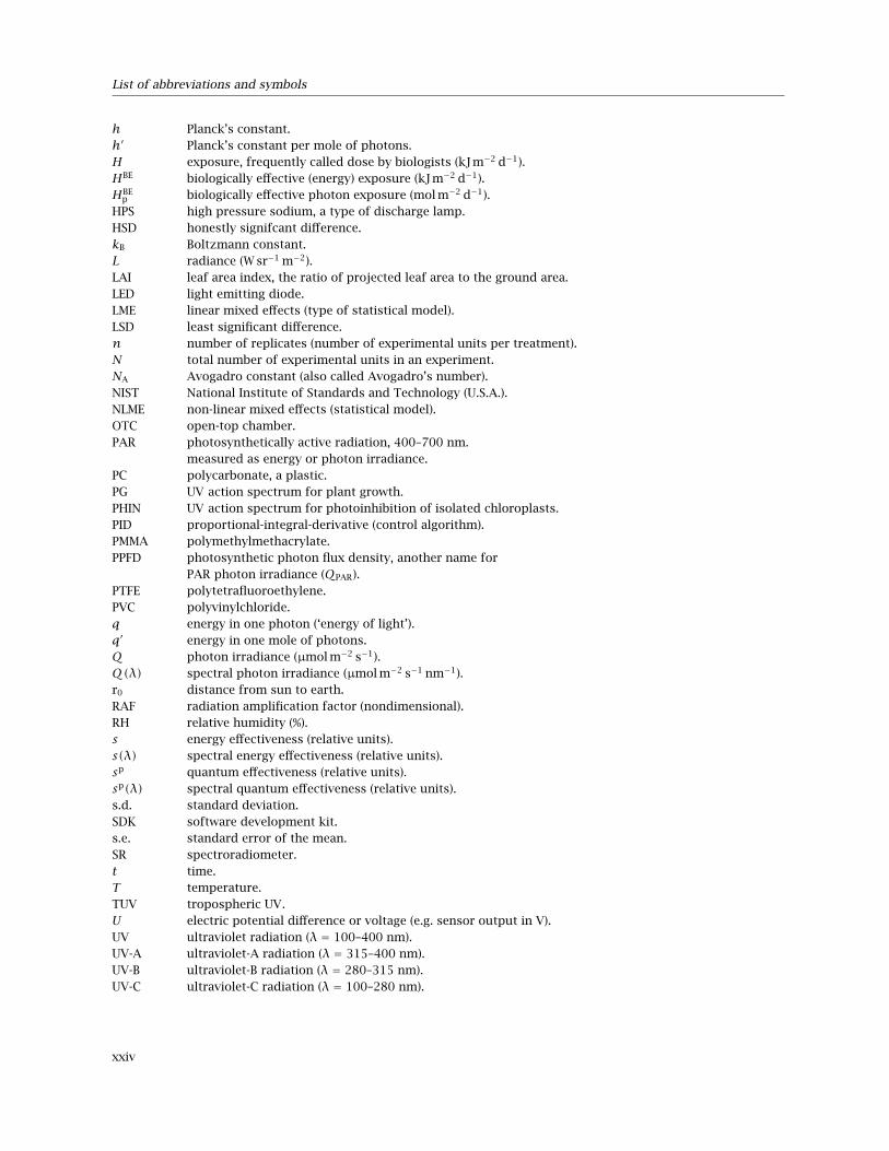
h Planck’s constant.h′ Planck’s constant per mole of photons.H exposure, frequently called dose by biologists (kJ m−2 d−1).HBE biologically effective (energy) exposure (kJ m−2 d−1).HBE

p biologically effective photon exposure (mol m−2 d−1).HPS high pressure sodium, a type of discharge lamp.HSD honestly signifcant difference.kB Boltzmann constant.L radiance (W sr−1 m−2).LAI leaf area index, the ratio of projected leaf area to the ground area.LED light emitting diode.LME linear mixed effects (type of statistical model).LSD least significant difference.n number of replicates (number of experimental units per treatment).N total number of experimental units in an experiment.NA Avogadro constant (also called Avogadro’s number).NIST National Institute of Standards and Technology (U.S.A.).NLME non-linear mixed effects (statistical model).OTC open-top chamber.PAR photosynthetically active radiation, 400–700 nm.

measured as energy or photon irradiance.PC polycarbonate, a plastic.PG UV action spectrum for plant growth.PHIN UV action spectrum for photoinhibition of isolated chloroplasts.PID proportional-integral-derivative (control algorithm).PMMA polymethylmethacrylate.PPFD photosynthetic photon flux density, another name for

PAR photon irradiance (QPAR).PTFE polytetrafluoroethylene.PVC polyvinylchloride.q energy in one photon (‘energy of light’).q′ energy in one mole of photons.Q photon irradiance (µmol m−2 s−1).Q(λ) spectral photon irradiance (µmol m−2 s−1 nm−1).r0 distance from sun to earth.RAF radiation amplification factor (nondimensional).RH relative humidity (%).s energy effectiveness (relative units).s(λ) spectral energy effectiveness (relative units).sp quantum effectiveness (relative units).sp(λ) spectral quantum effectiveness (relative units).s.d. standard deviation.SDK software development kit.s.e. standard error of the mean.SR spectroradiometer.t time.T temperature.TUV tropospheric UV.U electric potential difference or voltage (e.g. sensor output in V).UV ultraviolet radiation (λ = 100–400 nm).UV-A ultraviolet-A radiation (λ = 315–400 nm).UV-B ultraviolet-B radiation (λ = 280–315 nm).UV-C ultraviolet-C radiation (λ = 100–280 nm).

xxiv

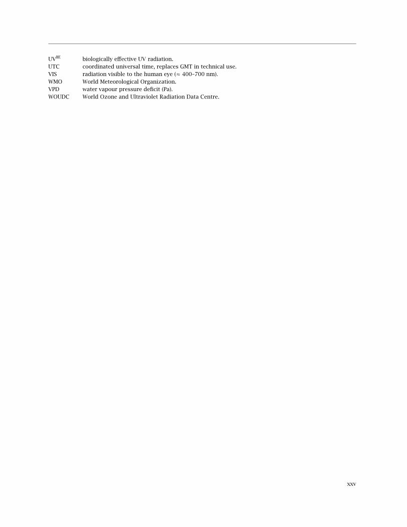
UVBE biologically effective UV radiation.UTC coordinated universal time, replaces GMT in technical use.VIS radiation visible to the human eye (≈ 400–700 nm).WMO World Meteorological Organization.VPD water vapour pressure deficit (Pa).WOUDC World Ozone and Ultraviolet Radiation Data Centre.

xxv

Preface

In this handbook we discuss methods relevant to researchon the responses of plants to ultraviolet (UV) radiation.We also summarize the knowledge needed to make in-formed decisions about manipulation and quantificationof UV radiation, and the design of UV experiments. Wegive guidelines and practical recommendations for ob-taining reliable and relevant data and interpretations. Wecover research both on terrestrial and aquatic plants (sea-weeds, marine angiosperms and freshwater higher plantsare included, but microalgae are excluded from the scopeof this work). We consider experimentation on ecological,eco-physiological and physiological questions.

The handbook will be most useful to early stage re-searchers (ESRs). However, more experienced researcherswill also find information of interest. The guidelinesthemselves, we hope, will ensure a high and uniformstandard of quality for UV research within our COST ac-tion, and the whole UV research community. We havewritten this text so that it is useful both for reading fromcover to cover and for reference. It will also be useful asa textbook for training workshops aimed at ESRs.

Physiological and eco-physiological experiments canattempt to respond to different objective questions: (1)will a future increase in UV radiation affect growth andmorphology of plants? (2) what is the effect of currentUV radiation levels on plant growth and morphology?(3) what are the mechanisms by which plants respondto UV radiation? Ecological experiments can have otherobjectives, e.g. (1) does UV radiation in sunlight affectplant fitness? (2) does a differential effect of UV radi-ation between plant species affect the outcome of com-petition? (3) does the exposure to UV radiation alterplant-pathogen and plant-herbivore interactions? Finallyapplied research related to agricultural and horticulturalproduction and produce is based on questions like: (1)can manipulations of UV radiation be used to manageproduce quality? (2) can manipulation of UV radiationreplace the use of pesticides and growth regulators? Theapproach suitable for a given experiment will depend onits objectives.

When doing experiments with terrestrial plants, themedium surrounding the stems and leaves is air. Atshort path lengths air has little influence on UV irradi-ance and only when considering the whole depth of theatmosphere, its UV transmittance needs to be taken into

account. In contrast, water and impurities like dissolvedorganic matter (DOM) absorb UV radiation over relativelyshort path lengths, which means that in water bodiesUV irradiance decreases with depth. Basic concepts ofphotobiology, radiation physics and UV in the naturalenvironment of plants are discussed in chapter 1.

Varied approaches are used in the study of the effectsof UV radition on plants. The main dichotomy is whether(1) UV radiation is added by means of special lamps toeither sunlight or to visible light from other lamps, or(2) UV radiation in sunlight is excluded or attenuatedby means of filters. Both approaches are extensivelydiscussed in chapter 2.

For any experimental approach used in UV research weneed to quantify UV radiation and express it as mean-ingful physical quantities that allow comparison amongexperiments and to natural conditions. When comparingUV irradiance from sources differing in spectral compos-ition, the comparison requires the calculation of biolo-gically effective doses. Quantification of UV radiation isdiscussed in chapter 3. The appendices present in detailthe calculations needed when measuring action spec-tra, and for calculating biologically effective UV dosesboth with Excel and R. An R package which facilitatessuch calculations accompanies this handbook, and willbe made available through CRAN (the ComprehensiveR Archive Network) and the handbook’s web pages athttp://uv4growth.dyndns.org.

Both for terrestrial and aquatic plants the enclosingmaterials should be carefully chosen based on their UVtransmittance and UV reflectance properties. This iscrucial in UV research, but also in any other researchwith plants using an enclosing structure such as open-top chambers (OTC), greenhouses or aquaria. These andmany other considerations about the cultivation of plantsare discussed in chapter 4.

Only experiments well designed from the statisticalpoint of view, allow valid conclusions to be reached. Inaddition a valid statistical analysis of the data, consistentwith the design of the experiment and based on as fewassumptions as possible, is required. Well designed ex-periments are also efficient in the use of resources (bothtime and money). The design of UV experiments and theanalysis of the data obtained are discussed in chapter 5.

Finally a few words about terminology. As the same

xxvii

Preface

quantities and units are used for measuring visible, andultraviolet radiation, throughout the book we use theword “radiation” to refer to both visible and ultravioletradiation. We prefer “radiation” to “light”, since light issometimes, but not always, used for just the portion ofthe electromagnetic spectrum visible to humans.

In the PDF file all links and crossreferences are ‘live’:just click on them to navigate through the file. They aremarked by coloured boxes in the viewer but these boxesare not printed. In the list of references DOIs and URLsare also hyperlinked.

If you find mistakes, or difficult to understand pas-sages, or have suggestions on how to improve this hand-book, please, send feedback directly to the lead ed-itor at mailto:pedro.aphalo@helsinki.fi?

subject=UVHandbookEdition01.The PDF file can be freely distributed and the latest

version will be available from the handbook web page athttp://uv4growth.dyndns.org/. Printed cop-ies can be obtained from http://www.amazon.co.uk, http://www.amazon.de or http://www.amazon.com.

Helsinki, Pedro J. AphaloMünchen, Andreas AlbertLund, Lars Olof BjörnEdinburgh, Andy McLeodHelsinki, T. Matthew RobsonCopenhagen, Eva Rosenqvist

October 2012

xxviii

Acknowledgements

The writing and publication of this book was made pos-sible by COST Action FA0906 ‘UV4growth’. This bookis a collaborative effort of all members of the technicalgroup on UV technology of this action, plus four authorsnot participating in the Action. The first conference andworkshop organized by the Action in Szeged, Hungary,put the authors in contact as well as allowing them torealise that a book on UV research methods was needed.Some of the authors met again in Denmark, and spenttwo and a half days of intense writing and discussionsthanks to the hospitality of Eva Rosenqvist and Carl-OttoOttosen. We thank Profs. Åke Strid and Donat Häderfor reading the whole manuscript and giving numeroussuggestions for improvement.

A preprint of this handbook was used in a trainingschool organised by the COST action at the University ofMálaga (16–18 April, 2012). Corrections of errors, sug-gestions for improvement and complains about difficultto understand passages from participants are acknow-ledged.

We thank Avantes (The Netherlands), BioSense (Ger-many), Biospherical Instruments Inc. (U.S.A.), Delta-T

Devices Ltd. (U.K.), EIC (Equipos Intrumentación y Con-trol) (Spain), Gooch & Housego (U.S.A.), Kipp & ZonenB.V. (The Netherlands), Ocean-Optics (The Netherlands),Valoya Oy (Finland) Skye Instruments Ltd. (U.K.), TriOSMess- und Datentechnik GmbH (Germany) and YankeeEnvironmental Systems, Inc. (U.S.A.) for providing illus-trations. We thank Prof. Donat Häder for supplying theoriginal data used to draw two figures and photographsof the ELDONET instrument. We thank Dr. Ulf Riebeselland Jens Christian Nejstgaard for photographs.

This work was funded by COST. Pedro J. Aphalo ac-knowledges the support of the Academy of Finland (de-cisions 116775 and 252548). Félix López Figueroa ac-knowledges the support by the Ministry of Innovationand Science of Spain (Project CGL08-05407-C03-01). AndyMcLeod acknowledges the support of a Royal SocietyLeverhulme Trust Senior Research Fellowship and re-search awards from the Natural Environment ResearchCouncil (U.K.). Iván Gómez and Pirjo Huovinen acknow-ledge the financial support by CONICYT (Chile) throughgrants Fondecyt 1090494, 1060503 and 1080171.

xxix

1 Introduction

Pedro J. Aphalo, Andreas Albert, Lars Olof Björn, Lasse Ylianttila, Félix López Figueroa, Pirjo Huovinen

1.1 Research on plant responses toultraviolet radiation

Plants are exposed to ultraviolet (UV) radiation in theirnatural habitats. The amount and quality of UV radiationthey are exposed to depends on the time of the year, thelatitude, the elevation, position in the canopy, cloudsand aerosols, and for aquatic plants the depth, solutesand particles contained in the water (see sections 1.4 and1.6). Ultraviolet radiation is consequently a carrier ofinformation about the environment of plants. However,when exposed to enhanced doses of UV radiation or UVradiation of short wavelengths, plants can be damaged.When exposed to small doses of UV-B radiation plantsrespond by a mechanism involving the perception of theradiation through a photoreceptor called UVR8 (Christieet al., 2012; Heijde and Ulm, 2012; Jenkins, 2009; Rizziniet al., 2011; D. Wu et al., 2012; M. Wu et al., 2011). Thisprotein behaves as a pigment at the top of a transductionchain that regulates gene expression. Several genes havebeen identified as regulated by UV-B radiation perceivedthrough UVR8. Some are related to the metabolism ofphenolic compounds and are involved in the accumula-tion of these metabolites.1 However, these are not theonly genes regulated by UVR8. Genes related to hormonemetabolism are also affected, and this could be one of themechanisms for photomorphogenesis by UV-B radiation,for example an increase in leaf thickness or reduction inheight of plants. Morphological effects of UV-B mediatedby UVR8 have been described (Wargent et al., 2009).

The irradiance of UV-A in sunlight is larger than theirradiance of UV-B and plants also have photoreceptorsthat absorb both UV-A radiation and blue light. The beststudied of these photoreceptors are cryptochromes andphototropins. Cryptochromes are involved in many pho-tomorphogenic responses, including the accumulation of

pigments. Phototropins are well known for their role inplant movements such as stomatal opening in blue lightand the movement of chloroplasts (see Christie, 2007;Möglich et al., 2010; Shimazaki et al., 2007, for recentreviews).

The balance between the different wavebands, UV-B,UV-A and PAR (photosynthetically active radiation, 400–700 nm), has a big influence on the effect of UV-B radi-ation on plants. Unrealistically low levels of UV-A radi-ation and PAR enhance the effects of UV-B (e.g. Caldwellet al., 1994). One reason for this is that UV-A radiation isrequired for photoreactivation, the repair of DNA damagein the light.

From the 1970’s until the 1990’s the main interest inresearch on the effects of UV-B on plants and other or-ganisms was generated by the increase in ambient UV-Bexposure caused by ozone depletion in the stratosphere(e.g. Caldwell, 1971; Caldwell and Flint, 1994b; Caldwell etal., 1989; Tevini, 1993). This led to many studies on the ef-fects of increased UV-B radiation, both outdoors, in green-houses and in controlled environments. Frequently theresults obtained in outdoor experiments differed fromthose obtained indoors. This lead to the realization that itis important to use realistic experimental conditions withrespect to UV-B radiation and its ratio compared to otherbands of the solar spectrum. Interactions of responsesto UV-B radiation with other environmental factors likeavailability of mineral nutrients, water and temperature,were also uncovered. Effects on terrestrial and aquaticecosystems of ozone depletion, and the concomitant in-crease in UV-B radiation, have been periodically reviewedin UNEP (2011, and earlier reports). These reports includechapters on terrestrial ecosystems (Ballaré et al., 2011)and aquatic ecosystems (Häder et al., 2011).

From the 1990’s onwards, the interest in the study ofthe effects of normal (i.e. without stratospheric ozone de-

1Many of these phenolics absorb UV radiation, so when they accumulate in the epidermis, they act as an UV shield (see Julkunen-Tiitto et al., 2005;Schreiner et al., 2012, for recent reviews). Other phenolics may behave as antioxidants (Julkunen-Tiitto et al., 2005; Schreiner et al., 2012).

1

1 Introduction

pletion), as opposed to enhanced UV radiation increasedmarkedly (e.g. Aphalo, 2003; Jansen and Bornman, 2012;Paul, 2001). This was in part due to the realization thateven low UV exposures elicit plant responses, and thatthese are important for the acclimation of plants to theirnormal growth environment. Furthermore, as these ef-fects were characterized, interest developed in their pos-sible applications in agriculture and especially horticul-ture (e.g. Paul et al., 2005).

A further subject of current interest is the enhancedrelease of greenhouse gases from green and dead bio-mass caused by action of UV radiation on pectins (e.g.Bloom et al., 2010; Messenger et al., 2009). Another long-standing subject of research are the direct and indirecteffects of solar UV radiation on litter decomposition (e.g.Austin and Ballaré, 2010; Newsham et al., 1997, 2001).

To be able to obtain reliable results from experimentson the effects of UV radiation on plants, there are manydifferent problems that need to be addressed. This re-quires background knowledge of both photobiology, ra-diation physics, and UV climatology.

1.2 The principles of photochemistry

Light is electromagnetic radiation of wavelengths towhich the human eye, as well as the photosyntheticapparatus, is sensitive (λ ≈ 400 to 700 nm). How-ever, sometimes the word light is also used to referto other nearby regions of the spectrum: ultraviolet(shorter wavelengths than visible light) and infra-red(longer wavelengths). Both particle and wave attributesof radiation are needed for a complete description of itsbehaviour. Light particles or quanta are called photons.

Sensing of visible and UV radiation by plants and otherorganisms starts as a photochemical event, and is ruledby the basic principles of photochemistry:

Grotthuss law Only radiation that is actually absorbedcan produce a chemical change.

Stark-Einstein law Each absorbed quantum activatesonly one molecule.

As electrons in molecules can have only discrete energylevels, only photons that provide a quantity of energyadequate for an electron to ‘jump’ to another possibleenergetic state can be absorbed. The consequence ofthis is that substances have colours, i.e. they absorbphotons with only certain energies. See Nobel (2009) andBjörn (2007) for detailed descriptions of the interactionsbetween light and matter.

1.3 Physical properties of ultraviolet andvisible radiation

In a physical sense, ultraviolet (UV) and visible (VIS) ra-diation (i.e. also PAR) are electromagnetic waves and aredescribed by the Maxwell’s equations.2 The wavelengthranges of UV and visible radiation and their usual namesare listed in Table 1.1. The long wavelengths of solarradiation, called infrared (IR) radiation, are also listed.The colour ranges indicated in Table 1.1 are an approx-imation. The electromagnetic spectrum is continuouswith no clear boundaries between one colour and thenext. Especially in the IR region the subdivision is some-what arbitrary and the boundaries used in the literaturevary. Radiation can also be thought of as composed ofquantum particles or photons. The energy of a quantumof radiation in a vacuum, q , depends on the wavelength,λ, or frequency3, ν ,

q = h · ν = h · cλ

(1.1)

with the Planck constant h = 6.626× 10−34 J s and speedof light in vacuum c = 2.998× 108 m s−1. When dealingwith numbers of photons, the equation (1.1) can be ex-tended by using Avogadro’s number NA = 6.022× 1023

mol−1. Thus, the energy of one mole of photons, q′, is

q′ = h′ · ν = h′ · cλ

(1.2)

with h′ = h · NA = 3.990 × 10−10 J s mol−1. Example 1:red light at 600 nm has about 200 kJ mol−1, therefore,1 µmol photons has 0.2 J. Example 2: UV-B radiationat 300 nm has about 400 kJ mol−1, therefore, 1 µmolphotons has 0.4 J. Equations 1.1 and 1.2 are valid for allkinds of electromagnetic waves.

When a beam or the radiation passing into a space orsphere is analysed, two important parameters are ne-cessary: the distance to the source and the measuringposition—i.e. if the receiving surface is perpendicular tothe beam or not. The geometry is illustrated in Figure1.1 with a radiation source at the origin. The radiationis received at distance r by a surface of area dA, tiltedby an angle α to the unit sphere’s surface element, socalled solid angle, dΩ, which is a two-dimensional anglein a space. The relation between dA and dΩ in sphericalcoordinates is geometrically explained in Figure 1.1.

The solid angle is calculated from the zenith angle θand azimuth angle φ, which denote the direction of theradiation beam

dΩ = dθ · sinθdφ (1.3)

2These equations are a system of four partial differential equations describing classical electromagnetism.3Wavelength and frequency are related to each other by the speed of light, according to ν = c/λ where c is speed of light in vacuum. Consequently

there are two equivalent formulations for equation 1.1.

2

1.3 Physical properties of ultraviolet and visible radiation

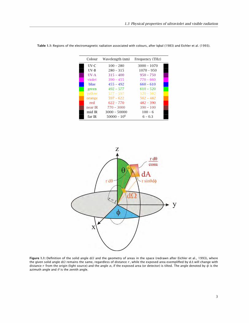
Table 1.1: Regions of the electromagnetic radiation associated with colours, after Iqbal (1983) and Eichler et al. (1993).

Colour Wavelength (nm) Frequency (THz)

UV-C 100 – 280 3000 – 1070UV-B 280 – 315 1070 – 950UV-A 315 – 400 950 – 750violet 390 – 455 770 – 660blue 455 – 492 660 – 610

green 492 – 577 610 – 520yellow 577 – 597 520 – 502orange 597 – 622 502 – 482

red 622 – 770 482 – 390near IR 770 – 3000 390 – 100mid IR 3000 – 50000 100 – 6far IR 50000 – 106 6 – 0.3

Figure 1.1: Definition of the solid angle dΩ and the geometry of areas in the space (redrawn after Eichler et al., 1993), wherethe given solid angle dΩ remains the same, regardless of distance r , while the exposed area exemplified by dA will change withdistance r from the origin (light source) and the angle α, if the exposed area (or detector) is tilted. The angle denoted by φ is theazimuth angle and θ is the zenith angle.

3

1 Introduction

The area of the receiving surface is calculated by a com-bination of the solid angle of the beam, the distance rfrom the radiation source and the angle α of the tilt:

dA = rdθcosα

· r sinθdφ (1.4)

which can be rearranged to

⇒ dA = r 2

cosαdΩ (1.5)

Thus, the solid angle is given by

Ω =∫A

dA · cosαr 2

(1.6)

The unit of the solid angle is a steradian (sr). The solidangle of an entire sphere is calculated by integration ofequation (1.3) over the zenith (θ) and azimuth (φ) angles,0 ≤ θ ≤ π(180) and 0 ≤ φ ≤ 2π(360), and is 4πsr. For example, the sun or moon seen from the Earth’ssurface appear to have a diameter of about 0.5 whichcorresponds to a solid angle element of about 6.8× 10−5

sr.The processes responsible for the variation of the ra-

diance L(λ, θ,φ) as the radiation beam travels throughany kind of material, are primarily absorption a and scat-tering b, which are called inherent optical properties,because they depend only on the characteristics of thematerial itself and are independent of the light field. Ra-diance is added to the directly transmitted beam, comingfrom different directions, due to elastic scattering, bywhich a photon changes direction but not wavelengthor energy level. An example of this is Raleigh scatteringin very small particles, which causes the scattering oflight in a rainbow. A further gain of radiance into thedirect path is due to inelastic processes like fluorescence,where a photon is absorbed by the material and reemittedas a photon with a longer wavelength and lower energylevel, and Raman scattering. The elastic and inelasticscattered radiance is denoted as LE and LI , respectively.Internal sources of radiances, LS , like bioluminescenceof biological organisms or cells contribute also to thedetected radiance. The path of the radiance through athin horizontal layer with thickness dz = z1−z0 is shownschematically in Figure 1.2.

Putting all this together, the radiative transfer equationis

cosθdLdz= −(a+ b) · L+ LE + LI + LS (1.7)

The dependencies of L on λ, θ, and φ are omitted herefor brevity. No exact analytical solution to the radiativetransfer equation exists, hence it is necessary either touse numerical models or to make approximations andfind an analytical parameterisation. A numerical model

is for example the Monte Carlo method. The parametersof the light field can be simulated by modelling the pathsof photons. For an infinite number of photons the lightfield parameters reach their exact values asymptotically.The advantage of the Monte Carlo method is a relativelysimple structure of the program, and it simulates naturein a straightforward way, but its disadvantage is the time-consuming computation involved. Details of the MonteCarlo method are explained for example by Prahl et al.(1989), Wang et al. (1995)4, or Mobley (1994).

The other way to solve the radiative transfer equationis through the development of analytical parameterisa-tions by making approximations for all the quantitiesneeded. In this case, the result is not exact, but it has theadvantage of fast computing and the analytical equationscan be inverted just as fast. This leads to the idealisedcase of a source-free (LS = 0) and non-scattering media,i.e. b = 0 and therefore LE = LI = 0. Then, equation 1.7can be integrated easily and yields

L(z1) = L(z0) · e−a·(z1−z0)

cosθ (1.8)

The boundary value L(z0) is presumed known. This res-ult is known as Beer’s law (or Lambert’s law, Bouguer’slaw, Beer-Lambert law), denotes any instance of expo-nential attenuation of light and is exact only for purelyabsorbing media—i.e. media that do not scatter radiation.It is of direct application in analytical chemistry, as itdescribes the direct proportionality of absorbance (A) tothe concentration of a coloured solute in a transparentsolvent.

Different physical quantities are used to describe the“amount of radiation” and their definitions and abbrevi-ations are listed in Table 1.2. Taking into account Equa-tion 1.6 and assuming a homogenous flux, the importantcorrelation between irradiance E and intensity I is

E = I · cosαr 2

(1.9)

The irradiance decreases by the square of the distanceto the source and depends on the tilt of the detectingsurface area. This is valid only for point sources. Foroutdoor measurements the sun can be assumed to bea point source. For artificial light sources simple LEDs(light-emitting diodes) without optics on top are alsoeffectively point sources. However, LEDs with optics—and other artificial light sources with optics or reflectorsdesigned to give a more focused dispersal of the light—deviate to various extents from the rule of a decreaseof irradiance proportional to the square of the distancefrom the light source.

Besides the physical quantities used for all electromag-netic radiation, there are also equivalent quantities to

4Their program is available from the website of Oregon Medical Laser Center at http://omlc.ogi.edu/software/mc/

4

1.3 Physical properties of ultraviolet and visible radiation

@@@R

@@@R@@

@@@

@@@

@@@@

v

v

-

-@@@R

z1

z0

Incoming radiance

L(θ,φ)

Loss by absorption a

and scattering b

Gain by elastic

scattered radiance

LE into the pathGain by inelastic scattered

radiance LI and internal

sources LS into the path

Outgoing radiance

L(θ,φ)

Figure 1.2: Path of the radiance and influences of absorbing and scattering particles in a thin homogeneous horizontal layer of airor water. The layer is separated from other layers of different characteristics by boundary lines at height z0 and z1.

Table 1.2: Physical quantities of light.

Symbol Unit Description

Φ = ∂q∂t W = J s−1 Radiant flux: absorbed or emitted energy per

time interval

H = ∂q∂A J m−2 Exposure: energy towards a surface area. (In

plant research this is called usually dose (H ),while in Physics dose refers to absorbed radi-ation.)

E = ∂Φ∂A W m−2 Irradiance: flux or radiation towards a surface

area, radiant flux density

I = ∂Φ∂Ω W sr−1 Radiant intensity: emitted radiant flux of a sur-

face area per solid angle

ε = ∂Φ∂A W m−2 Emittance: emitted radiant flux per surface area

L = ∂2Φ∂Ω(∂A·cosα) =

∂I∂A·cosα W m−2 sr−1 Radiance: emitted radiant flux per solid angle

and surface area depending on the angle betweenradiant flux and surface perpendicular

5

1 Introduction

Box 1.1: Photometric quantities

In contrast to (spectro-)radiometry, where the energy of any electromagnetic radiation is measured in terms ofabsolute power (J s = W ), photometry measures light as perceived by the human eye. Therefore, radiation isweighted by a luminosity function or visual sensitivity function describing the wavelength dependent response ofthe human eye. Due to the physiology of the eye, having rods and cones as light receptors, different sensitivityfunctions exist for the day (photopic vision) and night (scotopic vision), V(λ) and V ′(λ), respectively. Themaximum response during the day is at λ = 555 nm and during night at λ = 507 nm. Both response functions(normalised to their maximum) are shown in the figure below as established by the Commission Internationale del’Éclairage (CIE, International Commission on Illumination, Vienna, Austria) in 1924 for photopic vision and 1951for scotopic vision (Schwiegerling, 2004). The data are available from the Colour and Vision Research Laboratoryat http://www.cvrl.org. Until now, V(λ) is the basis of all photometric measurements.

Figure. Relative spectral intensity of human colour sensation during day (solid line)and night (dashed line), V(λ) and V ′(λ) respectively.

Corresponding to the physical quantities of radiation summarized in the table 1.2, the equivalent photometricquantities are listed in the table below and have the subscript v. The ratio between the (physiological) luminousflux Φv and the (physical) radiant flux Φ is the (photopic) photometric equivalent K(λ) = V(λ) ·Km with Km = 683lm W−1 (lumen per watt) at 555 nm. The dark-adapted sensitivity of the eye (scotopic vision) has its maximumat 507 nm with 1700 lm W−1. The base unit of luminous intensity is candela (cd). One candela is defined as themonochromatic intensity at 555 nm (540 THz) with I = 1

683 W sr−1. The luminous flux of a normal candle is around

12 lm. Assuming a homogeneous emission into all directions, the luminous intensity is about Iv = 12 lm4π sr ≈ 1 cd.

Table. Photometric quantities of light.

Symbol Unit Description

qv lm s Luminous energy or quantity of light

Φv = ∂qv∂t lm Luminous flux: absorbed or emitted luminous

energy per time interval

Iv = ∂Φv∂Ω cd = lm sr−1 Luminous intensity: emitted luminous flux of a

surface area per solid angle

Ev = ∂Φv∂A lux = lm m−2 Illuminance: luminous flux towards a surface

area

εv = ∂Φv∂A lux Luminous emittance: luminous flux per surface

area

Hv = ∂qv∂A lux s Light exposure: quantity of light towards a sur-

face area

Lv = ∂2Φv∂Ω(∂A·cosα) =

∂Iv∂A·cosα cd m−2 Luminance: luminous flux per solid angle and

surface area depending on the angle betweenluminous flux and surface perpendicular

6

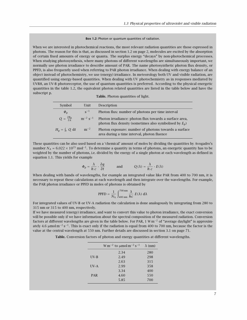
1.3 Physical properties of ultraviolet and visible radiation

Box 1.2: Photon or quantum quantities of radiation.

When we are interested in photochemical reactions, the most relevant radiation quantities are those expressed inphotons. The reason for this is that, as discussed in section 1.2 on page 2, molecules are excited by the absorptionof certain fixed amounts of energy or quanta. The surplus energy “decays” by non-photochemical processes.When studying photosynthesis, where many photons of different wavelengths are simultaneously important, wenormally use photon irradiance to describe amount of PAR. The name photosynthetic photon flux density, orPPFD, is also frequently used when referring to PAR photon irradiance. When dealing with energy balance of anobject instead of photochemistry, we use (energy) irradiance. In meteorology both UV and visible radiation, arequantified using energy-based quantities. When dealing with UV photochemistry as in responses mediated byUVR8, an UV-B photoreceptor, the use of quantum quantities is preferred. According to the physical energeticquantities in the table 1.2, the equivalent photon related quantities are listed in the table below and have thesubscript p.

Table. Photon quantities of light.

Symbol Unit Description

Φp s−1 Photon flux: number of photons per time interval

Q = ∂Φp∂A m−2 s−1 Photon irradiance: photon flux towards a surface area,

photon flux density (sometimes also symbolised by Ep)

Hp =∫t Q dt m−2 Photon exposure: number of photons towards a surface

area during a time interval, photon fluence

These quantities can be also used based on a ‘chemical’ amount of moles by dividing the quantities by Avogadro’snumber NA = 6.022× 1023 mol−1. To determine a quantity in terms of photons, an energetic quantity has to beweighted by the number of photons, i.e. divided by the energy of a single photon at each wavelength as defined inequation 1.1. This yields for example

Φp =λh c

· ∂q∂t

and Q(λ) = λh c

· E(λ)

When dealing with bands of wavelengths, for example an integrated value like PAR from 400 to 700 nm, it isnecessary to repeat these calculations at each wavelength and then integrate over the wavelengths. For example,the PAR photon irradiance or PPFD in moles of photons is obtained by

PPFD = 1NA

∫ 700 nm

400 nm

λhcE(λ) dλ

For integrated values of UV-B or UV-A radiation the calculation is done analogously by integrating from 280 to315 nm or 315 to 400 nm, respectively.If we have measured (energy) irradiance, and want to convert this value to photon irradiance, the exact conversionwill be possible only if we have information about the spectral composition of the measured radiation. Conversionfactors at different wavelengths are given in the table below. For PAR, 1 W m−2 of “average daylight” is approxim-ately 4.6 µmol m−2 s−1. This is exact only if the radiation is equal from 400 to 700 nm, because the factor is thevalue at the central wavelength at 550 nm. Further details are discussed in section 3.1 on page 71.

Table. Conversion factors of photon and energy quantities at different wavelengths.

W m−2 to µmol m−2 s−1 λ (nm)

2.34 280UV-B 2.49 298

2.63 315UV-A 2.99 358

3.34 400PAR 4.60 550

5.85 700

7

1 Introduction

describe visible radiation, so called photometric quantit-ies. The human eye as a detector led to these photometricunits, and they are commonly used by lamp manufactur-ers to describe their artificial light sources. See Box 1.1on page 6 for a short description of these quantities andunits.

There are, in principle, two possible approaches tomeasuring radiation. The first is to observe light fromone specific direction or viewing angle, which is the ra-diance L. The second is to use a detector, which sensesradiation from more than one direction and measures theso-called irradiance E of the entire sphere or hemisphere.The correlation between irradiance E and radiance L ofthe wavelength λ is given by integrating over all direc-tions of incoming photons.

E0(λ) =∫ΩL(λ,Ω)dΩ (1.10)

E(λ) =∫ΩL(λ,Ω)| cosα|dΩ (1.11)

Depending on the shape of a detector (which may beeither planar or spherical) the irradiance is called (plane)irradiance E or fluence rate (also called scalar irradiance)E0. A planar sensor detects incoming photons dependingon the incident angle and a spherical sensor detects allphotons equally weighted for all directions. See section3.1 on page 71 for a more detailed discussion.

Here we have discussed the properties of light basedon energy quantities. In photobiology there are goodreasons to quantify radiation based on photons. See Box1.2 on page 7, and section 3.1 on page 71.

1.4 UV in solar radiation

When dealing with solar radiation, we frequently need todescribe the position of the sun. The azimuth angle (φ)is measured clockwise from the North on a horizontalplane. The position on the vertical plane is measuredeither as the zenith angle (θ) downwards from the zenith,or as an elevation angle (h) upwards from the horizon.Consequently h+θ = 90 = π

2 radians. See Figure 1.3 fora diagram. In contrast to Figure 1.1 and the discussion insection 1.3 where the point radiation source is located atthe origin of the system of coordinates, when describingthe position of the sun as in Figure 1.3 the observer issituated at the origin.

Ultraviolet and visible radiation are part of solar radi-ation, which reaches the Earth’s surface in about eightminutes (t = time, r0 = distance sun to earth, c = velocityof light in vacuum):

t = r0

c≈ 150× 109 m

3× 108 ms

= 500 s = 8.3 min

The basis of all passive measurements is the incomingsolar radiation, which can be estimated from the knownactivity of the sun (‘productivity of photons’), that canbe approximated by the emitted spectral radiance (Ls)described by Planck’s law of black body radiation at tem-perature T , measured in degrees Kelvin (K):

Ls(λ, T) =2hc2

λ5· 1

e(hc/kBTλ)−1(1.12)

with Boltzmann’s constant kB = 1.381 × 10−23 J K−1.The brightness temperature of the sun can be determ-ined by Wien’s displacement law, which gives the peakwavelength of the radiation emitted by a blackbody as afunction of its absolute temperature

λmax · T = 2.898× 106 nm K (1.13)

This means that for a maximum emission of the sun atabout 500 nm the temperature of the sun surface is about5800 K. The spectral irradiance of the sun Es(λ) can beestimated assuming a homogeneous flux and using thecorrelation of intensity I and radiance L from their defin-itions in table 1.2. The intensity of the sun Is(λ) is givenby the radiance Ls(λ) multiplied by the apparent sunsurface (a non-tilted disk of radius rs = 7× 105 km). Tocalculate the decreased solar irradiance at the momentof reaching the Earth’s atmosphere, the distance of thesun to the Earth (r0 = 150× 106 km) has to be taken intoaccount due to the inverse square law of irradiance ofequation (1.9). Thus, the extraterrestrial solar irradianceis

Es(λ) = Ls(λ) ·πr 2

s

r 20

(1.14)

Remembering the solid angle of equation (1.6), the rightmultiplication factor represents the solid angle of thesun’s disk as seen from the Earth’s surface (≈ 6.8× 10−5

sr). Figure 1.4 shows the spectrum of the measuredextraterrestrial solar radiation (Wehrli, 1985)5 and thespectrum calculated by equation 1.14 using Planck’s lawof equation 1.12 at a black body temperature of 5800 K.Integrated over all wavelengths, Es is about 1361 to 1362W m−2 at top of the atmosphere (Kopp and Lean, 2011).This value is called the ‘solar constant’. In former times,depending on different measurements, Es varies by a fewpercent (Iqbal, 1983). For example, the irradiance at thetop of the atmosphere (the integrated value) changes by±50 W m−2 (3.7 %) during the year due to distance vari-ation caused by orbit excentricity (Mobley, 1994). Moreaccurate measurements during the last 25 years by space-borne radiometers show a variability of the solar radi-ation of a few tenth of a percent. A detailed analysisis given by Fröhlich and Lean (2004). Es can also be cal-culated by the Stefan-Boltzmann Law: the total energyemitted from the surface of a black body is proportional

5Available as ASCII file at PMODWRC, ftp://ftp.pmodwrc.ch/pub/publications/pmod615.asc

8

1.4 UV in solar radiation

North

ZenithSun

h

φ

θ

A

Figure 1.3: Position of the sun in the sky and the different angles used for its description by an observer located at point A. Theazimuth angle is φ, the elevation angle is h and the zenith angle is θ. These angles are measured on two perpendicular planes, onehorizontal and one vertical.

to the fourth power of its temperature. For an isotropic-ally emitting source (Lambertian emitter), this means

L = σπ· T 4 (1.15)

with the Stefan-Boltzmann constant σ = 5.6705× 10−8

W m−2 K−4. With T = 5800 K equation 1.15 gives theradiance of the solar disc. From this value, we can obtainan approximation of the solar constant, by taking intoaccount the distance from the Earth to the Sun and theapparent size of the solar disc (see equations 1.6 and1.9).

The total solar irradiance covers a wide range ofwavelengths. Using some of the ‘colours’ introducedin table 1.1, table 1.3 lists the irradiance and fraction ofEs of different wavelength intervals.

The extraterrestrial solar spectrum differs from thatat ground level due to the absorption of radiation by theatmosphere, because the absorption peaks of water, CO2

and other components of the atmosphere, cause corres-ponding valleys to appear in the solar spectrum at groundlevel. For example, estimates from measurements of thetotal global irradiance at Helmholtz Zentrum München(11.60 E, 48.22 N, 490 m above sea level) on two sunnydays (17th April 1996, sun zenith angle of 38 and 27th

May 2005, 27) result in about 5% for wavelengths below400 nm, about 45% from 400 to 700 nm, and about 50%above 700 nm. In relation to plant research, only thecoarse structure of peaks and valleys is relevant, becauseabsorption spectra of pigments in vivo have broad peaksand valleys. However, the solar spectrum has a muchfiner structure, due to emission and absorption lines ofelements, which is not observable with the spectrora-diometers normally used in plant research.

At the Earth’s surface, the incident radiation or globalradiation has two components, direct radiation andscattered or ‘diffuse’ radiation. Direct radiation is ra-

diation travelling directly from the sun, while diffuseradiation is that scattered by the atmosphere. Diffuseradiation is what gives the blue colour to the sky andwhite colour to clouds. The relative contribution of dir-ect and diffuse radiation to global radiation varies withwavelength and weather conditions. The contribution ofdiffuse radiation is larger in the UV region, and in thepresence of clouds (Figures 1.5 and 1.6).

Not only total irradiance, but also the wavelengthdistribution of the solar spectrum changes with theseasons of the year and time of day. The spectralwavelength distribution is also changed by the amountof UV-absorbing ozone in the atmosphere, known as theozone column. Figure 1.7 shows how spectral irradiancechanges throughout one day. When the whole spectrumis plotted using a linear scale the effect of ozone deple-tion is not visible, however, if we plot only the UV region(Figure 1.8) or use a logarithmic scale (Figure 1.9), theeffect becomes clearly visible. In addition, on a log scale,it is clear that the relative effect of ozone depletion onthe spectral irradiance at a given wavelength increaseswith decreasing wavelength.

Seasonal variation in UV-B irradiance has a larger rel-ative amplitude than variation in PAR (Figure 1.10). Thiscauses a seasonal variation in the UV-B: PAR ratio (Fig-ure 1.11). In addition to the regular seasonal variation,there is random variation as a result of changes in clouds(Figure 1.11). Normal seasonal and spatial variation inUV can be sensed by plants, and could play a role intheir adaptation to seasons and/or their position in thecanopy.

UV-B irradiance increases with elevation in mountainsand with decreasing latitude (Figure 1.12) and is particu-larly high on high mountains in equatorial regions. Thishas been hypothesized to be a factor in the determinationof the tree line6 in these mountains (Flenley, 1992).

6Tree line is the highest elevation on a mountain slope at which tree species are naturally able to grow.

9

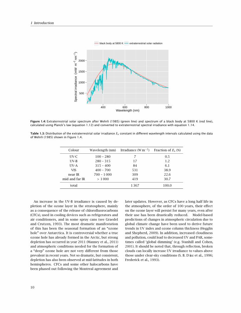
1 Introduction

500

1000

1500

2000

400 600 800 1000Wavelength (nm)

Spe

ctra

l irr

adia

nce

(mW

m−2

nm

−1)

black body at 5800 K extraterrestrial solar radiation

Figure 1.4: Extraterrestrial solar spectrum after Wehrli (1985) (green line) and spectrum of a black body at 5800 K (red line),calculated using Planck’s law (equation 1.12) and converted to extraterrestrial spectral irradiance with equation 1.14.

Table 1.3: Distribution of the extraterrestrial solar irradiance Es constant in different wavelength intervals calculated using the dataof Wehrli (1985) shown in Figure 1.4.

Colour Wavelength (nm) Irradiance (W m−2) Fraction of Es (%)

UV-C 100 – 280 7 0.5UV-B 280 – 315 17 1.2UV-A 315 – 400 84 6.1VIS 400 – 700 531 38.9

near IR 700 – 1 000 309 22.6mid and far IR > 1 000 419 30.7

total 1 367 100.0

An increase in the UV-B irradiance is caused by de-pletion of the ozone layer in the stratosphere, mainlyas a consequence of the release of chlorofluorocarbons(CFCs), used in cooling devices such as refrigerators andair conditioners, and in some spray cans (see Graedeland Crutzen, 1993). The most dramatic manifestationof this has been the seasonal formation of an “ozonehole” over Antarctica. It is controversial whether a trueozone hole has already formed in the Arctic, but strongdepletion has occurred in year 2011 (Manney et al., 2011)and atmospheric conditions needed for the formation ofa “deep” ozone hole are not very different from thoseprevalent in recent years. Not so dramatic, but consistent,depletion has also been observed at mid-latitudes in bothhemispheres. CFCs and some other halocarbons havebeen phased out following the Montreal agreement and

later updates. However, as CFCs have a long half life inthe atmosphere, of the order of 100 years, their effecton the ozone layer will persist for many years, even aftertheir use has been drastically reduced. Model-basedpredictions of changes in atmospheric circulation due toglobal climate change have been used to derive futuretrends in UV index and ozone column thickness (Hegglinand Shepherd, 2009). In addition, increased cloudinessand pollution, could lead to decreased UV and PAR, some-times called ‘global dimming’ (e.g. Stanhill and Cohen,2001). It should be noted that, through reflection, brokenclouds can locally increase UV irradiance to values abovethose under clear-sky conditions (S. B. Díaz et al., 1996;Frederick et al., 1993).

10

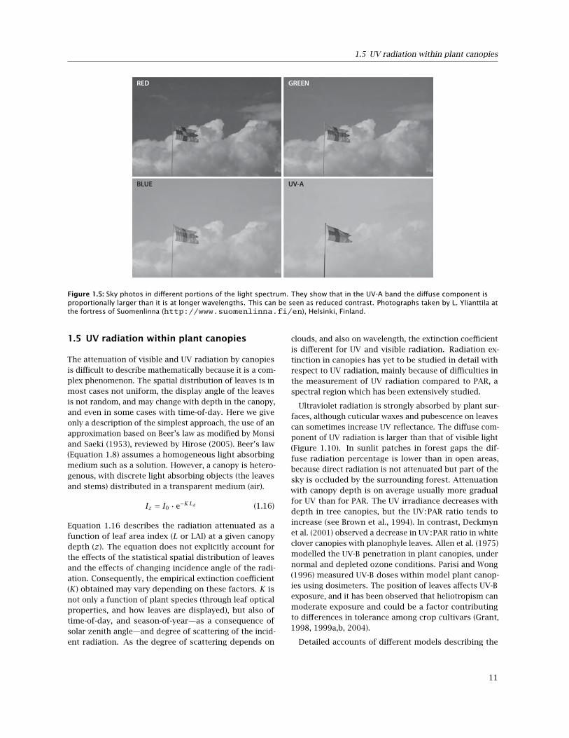
1.5 UV radiation within plant canopies

RED GREEN

BLUE UV-A

Figure 1.5: Sky photos in different portions of the light spectrum. They show that in the UV-A band the diffuse component isproportionally larger than it is at longer wavelengths. This can be seen as reduced contrast. Photographs taken by L. Ylianttila atthe fortress of Suomenlinna (http://www.suomenlinna.fi/en), Helsinki, Finland.

1.5 UV radiation within plant canopies

The attenuation of visible and UV radiation by canopiesis difficult to describe mathematically because it is a com-plex phenomenon. The spatial distribution of leaves is inmost cases not uniform, the display angle of the leavesis not random, and may change with depth in the canopy,and even in some cases with time-of-day. Here we giveonly a description of the simplest approach, the use of anapproximation based on Beer’s law as modified by Monsiand Saeki (1953), reviewed by Hirose (2005). Beer’s law(Equation 1.8) assumes a homogeneous light absorbingmedium such as a solution. However, a canopy is hetero-genous, with discrete light absorbing objects (the leavesand stems) distributed in a transparent medium (air).

Iz = I0 · e−K Lz (1.16)

Equation 1.16 describes the radiation attenuated as afunction of leaf area index (L or LAI) at a given canopydepth (z). The equation does not explicitly account forthe effects of the statistical spatial distribution of leavesand the effects of changing incidence angle of the radi-ation. Consequently, the empirical extinction coefficient(K) obtained may vary depending on these factors. K isnot only a function of plant species (through leaf opticalproperties, and how leaves are displayed), but also oftime-of-day, and season-of-year—as a consequence ofsolar zenith angle—and degree of scattering of the incid-ent radiation. As the degree of scattering depends on

clouds, and also on wavelength, the extinction coefficientis different for UV and visible radiation. Radiation ex-tinction in canopies has yet to be studied in detail withrespect to UV radiation, mainly because of difficulties inthe measurement of UV radiation compared to PAR, aspectral region which has been extensively studied.

Ultraviolet radiation is strongly absorbed by plant sur-faces, although cuticular waxes and pubescence on leavescan sometimes increase UV reflectance. The diffuse com-ponent of UV radiation is larger than that of visible light(Figure 1.10). In sunlit patches in forest gaps the dif-fuse radiation percentage is lower than in open areas,because direct radiation is not attenuated but part of thesky is occluded by the surrounding forest. Attenuationwith canopy depth is on average usually more gradualfor UV than for PAR. The UV irradiance decreases withdepth in tree canopies, but the UV:PAR ratio tends toincrease (see Brown et al., 1994). In contrast, Deckmynet al. (2001) observed a decrease in UV:PAR ratio in whiteclover canopies with planophyle leaves. Allen et al. (1975)modelled the UV-B penetration in plant canopies, undernormal and depleted ozone conditions. Parisi and Wong(1996) measured UV-B doses within model plant canop-ies using dosimeters. The position of leaves affects UV-Bexposure, and it has been observed that heliotropism canmoderate exposure and could be a factor contributingto differences in tolerance among crop cultivars (Grant,1998, 1999a,b, 2004).

Detailed accounts of different models describing the

11

1 Introduction

0.45

0.50

0.55

0.60

0.65

0.70

300 320 340 360 380 400 420Wavelength (nm)

Frac

tion

diffu

se d

ownw

ellin

g ra

diat

ion

0.0

0.2

0.4

0.6

0.8

1.0

300 320 340 360 380 400 420Wavelength (nm)

Spe

ctra

l irr

adia

nce

(W m

−2 n

m−1

)

Figure 1.6: Diffuse component in solar UV. Spectral irradiance of total downwelling radiation (lower panel, solid line), diffusedownwelling radiation (lower panel, long dashes), and ratio of diffuse downwelling to total downwelling spectral irradiance(upper panel, dashed line) are shown. Data from TUV model (version 4.1) for solar zenith angle = 4000′, cloud-free conditions,300 Dobson units. Simulations done with the Quick TUV calculator at http://cprm.acd.ucar.edu/Models/TUV/Interactive_TUV/.

04:30 08:30 12:30

200

400

600

800

1000

1200

300 500 700 300 500 700 300 500 700Wavelength (nm)

Spe

ctra

l irra

dian

ce (W

m−2

nm−1

)

Figure 1.7: The solar spectrum through half a day. Simulations of global radiation (direct plus diffuse radiation) spectral irradi-ance on a horizontal surface at ground level) for a hypothetical 21 May with cloudless sky at Jokioinen (6049’N, 2330’E), undernormal ozone column conditions. Effect of depletion is so small on the solar spectrum as a whole, that it would not visible in thisfigure. See Kotilainen et al. (2011) for details about the simulations.

12

1.5 UV radiation within plant canopies

11:30

100

200

300

400

500

300 310 320 330 340 350Wavelength (nm)

Spe

ctra

l irra

dian

ce (W

m−2

nm−1

)

20% ozone depletion normal ozone

Figure 1.8: The effect of ozone depletion on the UV spectrum of global (direct plus diffuse) solar radiation at noon. See fig. 1.7for details.

04:30 08:30 12:30

10−4

10−2

100

102

300 320 340 300 320 340 300 320 340Wavelength (nm)S

pect

ral i

rradi

ance

(W m

−2 n

m−1

)

20% ozone depletion normal ozone

Figure 1.9: The solar UV spectrum through half a day. The effect of ozone depletion on global (direct plus diffuse) radiation. Alogarithmic scale is used for spectral irradiance. See fig. 1.7 for details.

13

1 Introduction

0

20

40

60

80

100

8:00 12:00 16:00Time of day

Diff

use

perc

ent

0.0

0.2

0.4

0.6

0.8

1.0

0 100 200 300Day of year

Irrad

ianc

e at

noo

n (r

el. u

nits

)

Figure 1.10: UV-B and PAR. Left: Diffuse radiation as percentage of total (direct + diffuse) radiation in the UV-B (solid line) andPAR (dashed line) wavebands for open areas in a humid temperate climate under a clear sky. In cloudy conditions the percentageof diffuse radiation increases. Day of year not specified. Redrawn from Flint and Caldwell (1998). Right: Seasonal variation inmodelled, clear sky, solar-noon, UV-B (solid line) and PAR (dashed line) irradiance above the canopy for Maryland, USA. Irradianceexpressed relative to annual maximum of each waveband. Adapted from Brown et al. (1994).

0

1

2

3

4

5

1998 2000 2002 2004 2006Time (date)

UV

−B :

PAR

ene

rgy

ratio

(x 1

000)

0

10

20

30

40

1998 2000 2002 2004 2006Time (date)

UV

−B

(kJ

m−2

)

Figure 1.11: Seasonal variation in UV-B radiation at Erlangen, Germany (54 10’ N, 07 51’ E, 280 m asl). (Top) UV-B:PAR energyratio, calculated from daily exposures, and (bottom) UV-B daily exposure, measured with ELDONET instruments (see Figure 2 inHäder et al., 2007, for details).

14

1.6 UV radiation in aquatic environments

0

5

10

15

l

l

l

l

ll

l

l

l

lll

l

Abisk

oLund

Helg

olan

d

Rost

ock

Plym

outh

Erla

ngenKa

rlsru

he

Zugs

pitz

e

Pisa

Lisb

on

Athe

ns

Mál

aga

Gra

n Ca

naria

30 40 50 60 70Latitude N (degrees)

UV

−B

(M

J m

−2)

Figure 1.12: Latitudinal variation in UV-B radiation in the Northern hemisphere. UV-B annual exposure, measured with ELDONETinstruments (see Häder et al., 2007, for details).

interaction of radiation and plant canopies, taking intoaccount the properties of foliage, are given by Campbelland Norman (1998) and Monteith and Unsworth (2008).

1.6 UV radiation in aquatic environments

As solar radiation passes through a body of water, itsspectrum changes with depth in a wavelength-dependentmanner, determined by the optical characteristics of thatwater body. The penetration of UV radiation through wa-ter bodies can vary from only few centimetres in highlyhumic lakes (Huovinen et al., 2003; Kirk, 1994a,b) todozens of metres in the oceans (Kirk, 1994a,b; Smithet al., 1992). Some irradiance is reflected at the watersurface, but the extent to which wavelengths in the UVto IR range penetrate water bodies depends mainly on(1) attenuation by water itself, (2) coloured dissolved or-ganic matter (CDOM), and seston. Seston is the sum ofliving organic material (mainly phytoplankton) and non-living material (tripton). Non-living particles are furtherdistinguished between organic material (detritus) andinorganic suspended matter. Each fraction has its owncharacteristic spectral absorption and scattering proper-ties (reviewed by Dekker, 1993; Hargreaves, 2003; Kirk,1994a,b; Wozniak and Dera, 2007).

Particularly in coastal areas and shallow areas of lakesand streams, irradiance reflected from the ground or sea-bed beneath the water (henceforth bottom) influencesthe profile of radiation through the aquatic environment.This reflectance is described by a bidirectional reflectance

distribution function (BRDF), which is wavelength specificand depends on the incident and reflected angle. If thereflectance is equally distributed in all directions, the bot-tom is a so called Lambertian reflector and the BRDF isconstant. The bottom reflectance is greatly influenced byits slope and properties, i.e. whether the bottom is baresediment or covered by algae and submersed vegetation(e.g. Albert and Mobley, 2003; Maritorena et al., 1994;Mobley and Sundman, 2003; Mobley et al., 2003; Pinnel,2007).

1.6.1 Refraction

The refraction of incoming (downwelling) radiance at thewater surface can be determined by Snell’s law, whichdescribes the angular refraction of the incident beam.The radiation passes the first medium with a refractiveindex n1 and then the second medium with a refractiveindex n2. If the incoming direction of the radiation isgiven by the angle θ1, the beam is refracted to the angleθ2. Snell’s law is

n1 · sinθ1 = n2 · sinθ2 (1.17)

For the case of radiation arriving from the air under theincident angle θi and going into the water with the trans-mitted angle θt , this yields a refractive index for the airof na = 1 and for the water of nW = 1.33

θt = arcsin (0.75 · sinθi) (1.18)

Theoretically, nW is not constant but depends on tem-perature, wavelength and salinity, as described by Quan

15

1 Introduction

and Fry (1995). In principle, the shorter the wavelength,the higher the refractive index of water, but in practicethe wavelength-dependent difference in refraction is un-important. For example comparing the values at 400 and800 nm for 20C and no salinity produces a differenceof < 0.5%. If the wind speed is high, the slope of surfacewaves also has to be taken into account. A rough sur-face reflects and transmits the incoming radiation beamin more directions and makes the radiation field morediffuse than a smooth surface.

1.6.2 Absorption and scattering by pure water

Water itself absorbs and scatters radiation. The opticalproperties of the water in the visible and ultraviolet (UV)spectrum are not precisely known, since no theoreticalmodel exists which exactly describes the absorption andscattering properties of pure water. Therefore, it is ne-cessary to rely on laboratory measurements to approxim-ate the values of these parameters. Investigations intoabsorption by water aW were initially documented byMorel (1974), Smith and Tyler (1976), Smith and Baker(1981), Pegau and Zaneveld (1993) and more recently byBuiteveld et al. (1994) and Hakvoort (1994). The absorp-tion properties of water also depend on temperature. Theinfluence of temperature is weak below 700 nm, but itseffect increases with increasing wavelength; so, for ex-ample, a temperature increase of 10 K produces a ≈7%change in the absolute value of aW at 740 nm.

The scattering of radiation by molecules in liquids hasbeen modelled theoretically by Smoluchowski (1908) andEinstein (1910). This approach is based on statisticalthermodynamics and is called the theory of fluctuation.Theoretically, the scattering function is wavelength-dependent and follows the λ−4 law. Experiments showa slight deviation from the model, giving a better cor-relation with λ−4.32 (Morel, 1974) due to the effects ofisothermal compressibility, the refractive index of water,and the pressure derivative of the refractive index ofwater (Hakvoort, 1994).

The wavelength dependency of the absorption and scat-tering coefficients of pure water are shown in Figure 1.13using data from Hakvoort (1994). Water mainly contrib-utes to the attenuation of PAR and IR wavelengths, sinceabsorption by pure water increases from around 550 nmtowards longer wavelengths.

1.6.3 Absorption and scattering by waterconstituents

Absorption and scattering by water constituents is thesum of (1) absorption by CDOM, sometimes also calledyellow or humic substances, gilvin or gelbstoff, (2) absorp-tion and scattering by living material like phytoplankton,

and (3) absorption and scattering by dead organic andinorganic particles. The influence of each constituent onthe scattering process depends on wavelength, particlesize, concentration, and refractive index. Theoreticaldetails are explained in, for example, Hulst (1981).

CDOM mainly refers to coloured dissolved humic ma-terials and consists of humic and fulvic acids, originatingfrom decomposed plant material suspended in the wateror entering from the surrounding catchment area. Thepigments in humic and fulvic acids absorb strongly in theblue and UV wavelengths and are dissolved and thereforedo not scatter irradiance. Kalle (1966) recognised thatCDOM absorption decreases exponentially with increas-ing wavelength in the visible part of the spectra. Follow-ing the study of Morel and Prieur (1976), Bricaud et al.(1981) expressed this relationship in the following model:for a known absorption at a wavelength λ0 = 440 nm, theCDOM absorption aY can be determined by

aY (λ) = aY (λ0) · e−sY (λ−λ0) (1.19)

Although the exponential coefficient sY is variable, astandard value of sY = 0.014 nm−1 is commonly used.Bricaud et al. (1981) compared the value of sY acrossmany data sets and reported a standard deviation of only∆sY = ±0.003 nm−1. The amount of CDOM in water is de-termined by filtration using membrane filters of 0.2 µmpore size. The filtrate is collected into a quartz cuvettewith length l and put into a (double beam) spectrophoto-meter to measure its absorbance (optical density) A(λ).Then, aY (λ) = 2.303 · A(λ)l (Kirk, 1994a). The absorptioncoefficient at 440 nm has been used as an indicationof optical colour (Kirk, 1994a), while size of humic mo-lecules has been estimated from the ratio aY (λ=250nm)

aY (λ=365nm) ,with increasing size indicated by smaller ratios (Haan,1972, 1993; Haan et al., 1987). To determine aY fromclearer (e.g. oceanic) waters, a cuvette with a 10 cm path-length is generally needed due to their low values ofabsorption.

Phytoplankton can contribute to the attenuation ofPAR through absorption by their photosynthetic pig-ments such as chlorophyll and pheophytin, but they canalso cause scattering. The absorption by phytoplank-ton aP is the sum of absorption by each pigment mul-tiplied each by their concentrations. Due to the factthat many species of phytoplankton occur in aquatic en-vironments and every species contains more than onepigment, it is more practicable to calculate the absorp-tion by mean specific absorption coefficients for eachdifferent algal species separately. This has been done byGege (1998) for freshwater Lake Constance in Germanyand by Prieur and Sathyendranath (1981) for an oceanicenvironment. Besides these examples, there are othermodels for oceanic waters that use the specific in vivo

16

1.6 UV radiation in aquatic environments

10−3

10−2

10−1

100

400 500 600 700 800Wavelength (nm)

Spe

ctra

l abs

orpt

ion

or s

catte

ring

( m−1

)

absorption scattering

Figure 1.13: Absorption (red line) and scattering (green line) coefficients of pure water as a function of wavelength, after Hak-voort (1994). Shown in logarithmic scale.

absorption coefficient and concentration of chlorophyll-a, a∗chl and Cchl, respectively. Morel (1991) found thatthe power law aP = 0.06a∗chl [Cchl]0.65, which was firstproposed by Prieur and Sathyendranath (1981), providedthe best estimate of the absorption coefficient for hisdata set. Cchl is the concentration of chlorophyll-a inunits of µg l−1. Figure 1.14 shows the specific oceanicchlorophyll absorption coefficient from Morel (1991) nor-malized to maximum absorption at 440 nm. Figure1.14 also shows laboratory measurements of chlorophyll-a and chlorophyll-b absorption7 after Frigaard et al.(1996). Spectra for chlorophyll absorption, and that ofvarious other photochemically-relevant substances, arealso available in computer software such as Photochem-CAD8 (Dixon et al., 2005; Du et al., 1998). The empiricalmodel of Bricaud et al. (1995) parameterises the spe-cific absorption coefficient from Cchl. This model drawson extensive studies of more than 800 spectra to givea∗P (λ) = A(λ)[Cchl]−B(λ) with positive empirical coeffi-cients A and B depending on wavelength. The modelincorporates both the package effect of phytoplanktoncells and the effect of the varying pigment compositionon absorption.

The particulate structure of phytoplankton cells causesscattering. The influence of phytoplankton on the totalscattering coefficient depends on the other constituents

of the water body. For water containing a low concentra-tion of inorganic suspended sediment scattering is drivenby the concentration of phytoplankton (as occurs in theopen ocean). Gordon and Morel (1983) developed an em-pirical model, which directly correlates scattering withthe pigment concentration of chlorophyll-a Cchl in unitsof µg l−1. The scattering coefficient of phytoplankton bPin units of m−1 is given by

bP (λ) = B · [Cchl]0.62 ·(λ0

λ

)(1.20)

with λ0 = 550 nm and B = 0.3 as mean values for oceanicwaters dominated by phytoplankton. The equation (1.20)is valid for a range of phytoplankton concentrations from0.05 to 1 µg l−1. Gordon and Morel (1983) found thatoceanic waters have a value of B ≤ 0.45. Higher valuesare used for other aquatic environments, for exampleturbid coastal waters. In coastal regions, Sathyendranathet al. (1989) proposed that the scattering coefficient isindirectly proportional to absorption by phytoplankton:bP (λ)∝ 1/aP (λ). The proportionality factor depends onthe concentration of chlorophyll-a in the same manneras the scattering coefficient of equation (1.20). Dekker(1993) investigated the contribution to scattering of eachwater constituent in inland waters9. He found that thecomposition of scattering particles was more variable ininland waters than in the ocean and it depended on the

7Data available from Frigaard’s website at the University of Copenhagen at http://www.bio.ku.dk/nuf/resources/scitab/chlabs/index.htm.

8Latest software version available at the PhotochemCAD website at http://photochemcad.com. Data available at the PhotochemCAD datasite at http://omlc.ogi.edu/spectra/PhotochemCAD/index.html.

9Inland waters include rivers, streams and lakes.

17

1 Introduction

trophic state of the water and therefore on the distri-bution of organic and inorganic particulate matter. Thescattering and backscattering coefficient of phytoplank-ton can be determined by bP (λ) = b∗P (λ) · CP where thespecific scattering coefficient of phytoplankton is b∗P . Forlakes Dekker (1993) reported that the specific scatteringcoefficient of phytoplankton ranges from 0.12 to 0.18m2mg−1 at a wavelength of 550 nm. The specific scat-tering coefficients can be obtained by integrating thescattering phase function of the observed matter, here,phytoplankton. Extensive and commonly used measure-ments were done by Petzold (1977). Other functions canbe found for example in Mobley (1994).

Particulate matter in water bodies consists of organicand inorganic material. The organic constituents are con-tained in phytoplankton cells or are fragments of deadplankton and faecal pellets of zooplankton. These partsare often called detritus. Inorganic particles include sus-pended mineral coming from inflows or resuspensionat coastal regions. They mainly consist of quartz, clay,and calcite. There are only a few published values of thespecific absorption coefficients of suspended particles inwater from aquatic environments because they are dif-ficult to separate into their individual constituent parts.A comparison of these values is given by Pozdnyakovand Grassl (2003). In general, absorption by all suspen-ded particles in most water bodies is very low and it isnegligible for inorganic particles. Roesler et al. (1989)produced the following relationship for absorption bydetritus in coastal waters which is very similar that ofCDOM:

aX(λ) = aX(λ0) · e−sX (λ−λ0) (1.21)

with a mean value of sX = 0.011 nm−1 and aX(λ0) = 0.09m−1 at λ0 = 400 nm for their data. Particulate matterin general causes more scattering of irradiance than itabsorbs. In coastal waters and freshwater, scattering ishigher than in oceanic waters due to the additional pres-ence of particles not related to phytoplankton. Theseparticles come from suspended inorganic sediments ofdifferent sizes. Scattering is caused by differences in therefractive indices of the two materials (the water mediumand the material of the particles) and are due to the ra-tio of particle size to wavelength. Different functions ofscattering coefficients and phase functions are, for ex-ample, described by Mobley (1994). Especially turbid andcoastal waters, or rivers and lakes, are dominated by largeparticles (> 1 µm and a refraction index of 1.03). There-fore, the scattering coefficient of non-living particles bXcan be estimated while neglecting their size distributionand wavelength dependence. Thus, bX is derived frombX(λ) = b∗X · CX , with the concentration of the total sus-pended matter CX and the specific scattering coefficientsb∗X . Dekker (1993) gave example specific scattering coef-

ficients of 0.23 to 0.79 m2 g−1 for different trophic statesin lakes.

1.6.4 Results and effects

In summary, after considering all the components thatabsorb radiation, in very clear non-productive oceanicwaters blue-green wavelengths in the PAR spectrum dom-inate, whereas in highly-coloured, humic inland watersblue wavelengths are rapidly attenuated. In humic lakes,CDOM largely governs UV attenuation (e.g. Huovinen etal., 2003; Kirk, 1994a,b; Scully and Lean, 1994)), whereasin oceans (Smith and Baker, 1979) and clear lakes con-taining low CDOM concentrations the contribution ofphytoplankton to UV attenuation can be significant (Som-maruga and Psenner, 1997). If very turbid water containsa large amount of inorganic particles, CDOM is bondedby calcium carbonate contained in the particles, and con-sequently the colour of the water returns to blue.

There is marked variation in the penetration of UVradiation among water bodies, and within a water bodyduring the year. Global changes, such as climate warmingand acidification (Donahue et al., 1998; Schindler et al.,1996; Yan et al., 1996) can lead to increased underwaterUV penetration, likewise UV-B radiation itself which canpositively affect its own penetration through the pho-todegradation of CDOM (Morris and Hargreaves, 1997).Variation in the absorption properties of dissolved or-ganic compounds with the seasons and according to theirorigin and molecular weight (Hessen and Tranvik, 1998;Lean, 1998; Stewart and Wetzel, 1980), interferes with ourestimation of UV penetration based on CDOM concentra-tions. Temporal changes in the absorption characteristicsof CDOM have also been reported, with fresh CDOM be-ing photochemically more active than older CDOM (Lean,1998). It is also notable that UV radiation has been shownto penetrate deeper in saline prairie lakes than in freshwaters of corresponding CDOM concentrations (Arts etal., 2000).

Estimations of CDOM are relatively easy to performand therefore often used for in situ and remote sensingmeasurements of optical properties. However, anotherparameter called dissolved organic carbon (DOC, in unitsof mg l−1) is also useful to measure, since it is more inter-pretable for studies of carbon cycling and in the contextof global change research. Kowalczuk et al. (2010), reportthat CDOM contributes approximately 20% to the totalDOC pool in the open ocean and up to 70% in coastalareas. Unfortunately, on a global scale it has not yet beenpossible to make a direct link between CDOM and DOCdue to the heterogeneous organic composition of CDOM.Until that connection is made, estimation of the univer-sal bulk carbon-specific CDOM absorption coefficient,defined as the ratio of CDOM absorption to DOC concen-

18

1.6 UV radiation in aquatic environments

0.0

0.2

0.4

0.6

0.8

1.0

300 400 500 600 700 800Wavelength (nm)

Coe

ffici

ent o

f abs

orpt

ion

(rel

ativ

e un

its)

Chl a Chl b Phytoplankton

Figure 1.14: Specific oceanic chlorophyll absorption spectrum, after Morel (1991), normalized to maximum absorption at 440 nm(blue line), and absorption spectra of chlorophyll-a (normalized at 428 nm, red line) and chlorophyll-b (normalized at 436 nm,green line) dissolved in diethyl ether, after Frigaard et al. (1996).

tration, remains almost impossible (Wozniak and Dera,2007), but at least there are good correlations betweenaY and DOC concentrations in coastal areas (Kowalczuket al., 2010).

Aquatic organisms can be affected not only directlybut also indirectly through UV-dependent changes in thesurrounding water, e.g. through increased formation ofphotochemical reaction products such as singlet oxygenand hydrogen peroxide. Especially in lakes with low DOCconcentrations, photoenhanced toxicity of some envir-onmental contaminants or release of complexed metalsinto the water can occur due to the photodegradation oforganic matter (Arfsten et al., 1996; Hessen and Donk,1994; Palenik et al., 1991; Scully et al., 1997; Zepp, 1982).Despite the potential for detrimental effects, the finalimpact of UV radiation on organisms may be mitigatedby their protective and repair mechanisms (Karentz et al.,1991; Mitchell and Karentz, 1993; Vincent and Roy, 1993),which somehow also depend on certain wavelengths ofirradiation. When evaluating the exposure of seaweeds toUV radiation, it should be taken into account that otherfactors, such as kelp canopies, can markedly reduce thePAR and UV radiation reaching their understorey. Fur-thermore, the underwater radiation received by seaweedscan be significantly altered depending on the tidal range(Huovinen and Gómez, 2011). Phenolic compounds re-leased from large brown algae into the surrounding watercan also locally attenuate UV radiation.

Classifications of water bodies based on their opticalcharacteristics have been developed as general tools in or-

der to allow comparisons between different water bodies.Jerlov (1976) traditional and widely-used classification ofmarine waters, based on their transmittance of irradianceat different wavelengths, recognizes three oceanic (I–III)and nine coastal (1–9) types of water body (Figure 1.15).Morel and Prieur (1977) classified ocean waters into twotypes based on their optically dominant components: (i)phytoplankton and their products dominate case-i waters,(ii) particles and dissolved coloured material dominatecase-ii waters. The classification proposed by Kirk (1980)is principally suited to inland waters and is based on thespectral absorption of the soluble and particulate frac-tions. Kirk (1980) defined type G waters, in which CDOMis the dominant light-absorbing component, comparedwith type T, W and A waters, where tripton, water itselfand phytoplankton dominate respectively. Beyond thesescales, various other optical classifications have also beenproposed (reviewed by Hargreaves, 2003; Kirk, 1994a).

1.6.5 Modelling of underwater radiation

Following Beer’s law (Equation 1.8), for deep water (noreflection from bottom), radiance L(λ) decreases expo-nentially with depth z in the water column:

L(z, λ) = L(z = 0, λ) · e−a·z

cosθ (1.22)

alternatively written as

cosθdL(z, λ)

dz= −a · L(z, λ) (1.23)

19

1 Introduction

Figure 1.15: Optical classification of marine waters (based on transmittance of irradiance) according to Jerlov’s oceanic (I–III) andcoastal (1–9) classification system (redrawn from Jerlov, 1976).

θ is the zenith angle of the incoming (downwelling) ra-diance in water. Note that Eqs. 1.22 and 1.23 are onlyvalid if the water column is homogeneous with depthand there are no scattering particles and internal sourcesof light in the water, i.e. no fluorescence, raman scat-tering, nor bioluminescence. Thus, calculation of actualradiative transfer in water (not under idealised condi-tions) is much more complicated and can only be solvedapproximately by using empirical, semi-analytical or com-putational models (Albert and Gege, 2006; Dekker, 1993;Lee et al., 2002; Mobley, 1994).

The radiative transfer equations 1.22 and 1.23 are validfor radiance L, which represents the collimated beamfrom one specific direction. Due to their construction,radiance detectors do not measure a beam from an infin-itely small solid angle, they have an aperture of typicallyone or two degrees. Other types of detectors sense lightfrom more than one direction, they measure the entiresphere or hemisphere (for details see also section 3.1on page 71), by integrating the incoming radiance overall directions. Another useful relationship between irra-diance E and fluence rate E0 can be obtained using theGershun equation:

ddzE(z, λ) = −aE0(z, λ) (1.24)

If, for example, only the downwelling irradiance Ed(z, λ)is measured or necessary for calculating radiative trans-fer, Equation 1.23 yields

dEd(z, λ)dz

= −Kd · Ed(z, λ) (1.25)

giving the diffuse attenuation coefficient for downwellingirradiance, Kd. Kd is related to the total absorption a

and scattering b as well as to θ and also the solar zenithangle θs (Albert and Mobley, 2003; Kirk, 1991). A practicaland often-used method to estimate Kd, and therefore thetransparency of the water, is the Secchi disk test. Thevisibility of a submerged white disk can be correlatedto downwelling diffuse attenuation (Tyler, 1968). Thisand also the penetration depth zd give useful inform-ation about the water body. The penetration of irradi-ance important for photosynthesis (primary production)is often expressed as the depth at which, for example,1% or 10% of the value just below the water surface isreached. The depth, where 1% of PAR is reached, separ-ates the euphotic zone from the aphotic zone. After Kirk(1994a), zd can be obtained from Kd: zd(1%) = 4.6/Kdand zd(10%) = 2.3/Kd. In Figure 1.16, an example ofspectral attenuation of solar radiation at different depths,as well as the penetration depths of UV-B, UV-A radiationand PAR are given for coastal waters of the south-easternPacific Ocean (off the coast of Chile).

A very useful tool to simulate spectral radiance andirradiance under water, depending on different concen-trations of the water constituents or bottom depth andtype, is called WASI (water colour simulator, Gege, 2004).The software includes different analytical parameterisa-tions and it can also be used for inverse calculations, i.e.for estimating optical properties and concentrations ofwater constituents from (remote sensing) measurements.The software program including the manual is availablefree of charge using an anonymous login at the ftp serverftp://ftp.dfd.dlr.de/pub/WASI. Other mod-els, which include angular distributions of radiation un-der water are, for example, the Monte Carlo method (Prahl

20

1.7 UV radiation within plant leaves

et al., 1989; Wang et al., 1995)10, HydroLight (techniquedescribed by Mobley, 1994), or EcoLight-S (Mobley, 2011).

1.7 UV radiation within plant leaves

Modelling of UV-B within plant leaves has not so farbeen successfully achieved. For empirical estimationsof UV penetration two methods have mainly been used:fibre-optic measurements and UV-induced fluorescence.Neither of them is ideal and both give only partial inform-ation.

1.7.1 Fibre-optic measurements

This method was introduced for visible light by Vogel-mann and Björn (1984), and has been adapted for ultra-violet radiation by Vogelmann, Bornman and coworkers(Bornman and Vogelmann, 1988; Cen and Bornman, 1993;DeLucia et al., 1992). The method cannot be used for ab-solute measurements due to uncertainties about the localconditions and the acceptance angle at the fibre tip, butit has yielded valuable comparisons between wavelengthsand depth distributions of radiation. Fibre probes can bemade more angle-independent (García-Pichel, 1995), butthen become too bulky for measurements inside plantleaves.

1.7.2 UV-induced chlorophyll fluorescence

This method has so far only been employed by excitationand measurement at the leaf surface. It thus mainly mon-itors penetration of UV radiation through the epidermisinto the chlorophyll-containing mesophyll, i.e. transmis-sion through the epidermis (Figure 1.17). Chlorophyllfluorescence excited by blue light usually serves as astandard (Bilger et al., 2001, 1997), more recently excita-tion by red light has also been used to avoid interferenceby anthocyanins (Goulas et al., 2004). The principle hasbeen used in commercial instruments that assess the UVabsorbance of the epidermis (Goulas et al., 2004; Kolb etal., 2005). The first portable instruments, UVA-PAM andDualex FLAV used UV-A radiation for excitation ratherthan UV-B radiation, but now there is at least one instru-ment, Dualex HCA, measuring UV-B absorbance.

In principle, chlorophyll fluorescence could also beused for monitoring UV penetration in another way, byrecording fluorescence in cross-sections of leaves, as hasalready been done for the penetration of visible light(Gould et al., 2002; Vogelmann and Evans, 2002; Vogel-mann and Han, 2000).

1.7.3 Factors affecting internal UV levels

Many studies have indicated that UV-absorbing com-pounds in the vacuoles of epidermal cells have a majorrole in regulating internal UV levels. However, absorb-ing compounds located in cell walls and other cell partscan also be important in controlling internal UV penet-ration. These compounds are usually not easily extract-able, and consequently one cannot rely on extracts alonewhen judging the effectiveness of UV-screening protec-tion. Furthermore, both wax deposits and pubescencemay be very important for protection against ultravioletradiation (Holmes and Keiller, 2002; Karabourniotis andBornman, 1999). The amount of UV protection can alsovary over time, even during the day, probably as a res-ult of changes in flavonoid concentrations (Barnes et al.,2008; Veit et al., 1996). Of course leaf properties confer-ring protection also depend on environmental factors,in particular prior UV-B exposure, and great differencesexist among plant species.

1.8 Action and response spectra

Plants do not respond equally to all wavelengths of UV,and this spectral response can be described by a responsespectrum and/or by an action spectrum. It is importantto be aware that an action spectrum is not the same thingas a response spectrum. Although they are both usedto describe the wavelength dependency of a biologicalresponse to radiation they are measured and used differ-ently. Because they are measured in different ways theyyield curves of different shapes. A response spectrumshows the size of the response at a fixed photon fluence11

of radiation across a series of different wavelengths. How-ever, since UV radiation never comes at fixed irradiancesover the entire spectrum the response spectrum is of lim-ited use when estimating the physiological response tosolar- or broadband UV exposure. In contrast, an actionspectrum shows the effectiveness of radiation of differentwavelengths in achieving a given size of response. Thisis a very important difference because dose responsecurves are not necessarily parallel or linear.

When estimating biologically effective irradiances (seesection 3.10 on page 99) it is very important to useappropriate action spectra for each biological process.However, since the action spectra of many biologicalresponses are not known, this provides a dilemma for re-searchers who must try to chose the action spectrum thatbest approximates the process they are studying. Usingthe wrong action spectrum can produce very large errors

10Program available from the website of the Oregon Medical Laser Center at http://omlc.ogi.edu/software/mc/11Different values of photon fluence can be obtained either by varying the irradiance, or the irradiation time. However, if the irradiation time is

varied it is important to check that reciprocity holds. In other words, that the same fluence achieved through different irradiation times elicitsthe same size of response.

21

1 Introduction

Fig

ure

1.1

6:Ex

ample

of

the

underw

aterirrad

iance

ina

coastal

systemin

the

Pacific

Ocean

off

south

ernC

hile

(coast

of

Vald

ivia).

22

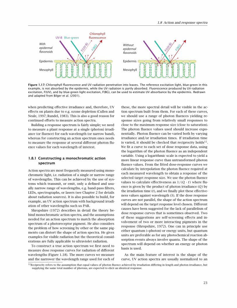
1.8 Action and response spectra

F(UV-B)

UV-B Blue-greenChlorophyllfluorescence

F(BG)

Epidermis

Mesophyll

F(UV-B)

F(BG)

Epidermis

Mesophyll

Withepidermalflavonoids

Withoutepidermalflavonoids

Figure 1.17: Chlorophyll fluorescence and UV radiation penetration into leaves. The reference excitation light, blue-green in thisexample, is not absorbed by the epidermis, while the UV radiation is partly absorbed. Fluorescence produced by UV-radiationexcitation, F(UV), and by blue-green light excitation, F(BG), can be used to estimate UV absorbance by the epidermis. Redrawnand adapted from Bilger et al. (2001).

when predicting effective irradiance and, therefore, UVeffects on plants due to e.g. ozone depletion (Cullen andNeale, 1997; Rundel, 1983). This is also a good reason forcontinued efforts to measure action spectra.

Building a response spectrum is fairly simple; we needto measure a plant response at a single (photon) irradi-ance (or fluence) for each wavelength (or narrow band),whereas for constructing an action spectrum ones needsto measure the response at several different photon flu-ence values for each wavelength of interest.

1.8.1 Constructing a monochromatic actionspectrum

Action spectra are most frequently measured using mono-chromatic light, i.e. radiation of a single or narrow rangeof wavelengths. This can be achieved by the use of sys-tems which transmit, or emit, only a defined and usu-ally narrow range of wavelengths, e.g. band-pass filters,LEDs, spectrographs, or lasers (see Chapter 2 for detailsabout radiation sources). It is also possible to build, forexample, an UV action spectrum with background irradi-ation of other wavelengths such us PAR.

Shropshire (1972) describes in detail the theory be-hind monochromatic action spectra, and the assumptionsneeded for an action spectrum to match the absorptionspectrum of a photoreceptor pigment. He also considersthe problem of how screening by other or the same pig-ments can distort the shape of action spectra. He givesexamples for visible radiation but the theoretical consid-erations are fully applicable to ultraviolet radiation.

To construct a true action spectrum we first need tomeasure dose response curves for radiation of differentwavelengths (Figure 1.18). The more curves we measureand the narrower the wavelength range used for each of

these, the more spectral detail will be visible in the ac-tion spectrum built from them. For each of these curves,we should use a range of photon fluences yielding re-sponse sizes going from relatively small responses toclose to the maximum response size (close to saturation).The photon fluence values used should increase expo-nentially. Photon fluence can be varied both by varyingirradiance and/or irradiation times. If irradiation timeis varied, it should be checked that reciprocity holds12.We fit a curve to each set of dose response data, usingthe logarithm of the photon fluence as an independentvariable. Using a logarithmic scale is expected to yield amore linear response curve than untransformed photonfluence values. From the fitted dose-response curves wecalculate by interpolation the photon fluence required ateach measured wavelength to obtain a response of theselected target response size. We use the photon fluencevalues to calculate effectiveness as 1/(Q · t) where flu-ence is given by the product of photon irradiance (Q) bythe irradiation time (t), and we finally plot these effective-ness values against wavelength (λ). If the dose responsecurves are not parallel, the shape of the action spectrumwill depend on the target response level chosen. Differentcauses have been suggested for the lack of parallelism ofdose response curves that is sometimes observed. Twoof these suggestions are self-screening effects and in-volvement of two or more interacting pigments in theresponse (Shropshire, 1972). One can in principle useeither quantum (=photon) or energy units, but quantumunits are preferable as for any photochemical reaction ab-sorption events always involve quanta. The shape of thespectrum will depend on whether an energy or photonbasis is used.

As the main feature of interest is the shape of thecurve, UV action spectra are usually normalized to an

12Reciprocity refers to the assumption that equal values of photon fluence achieved by irradiation differing in length and photon irradiance, butsupplying the same total number of photons, are expected to elicit an identical response.

23

1 Introduction

0.5

0.6

0.7

0.8

0.9

1.0

10−1 100 101 102 103

Photon fluence (µmol m−2)

Res

pons

e (r

elat

ive

units

)

Wavelength (nm) 290 315 340 360 400

Figure 1.18: Hypothetical example of dose response curves at different wavelengths. The horizontal dashed line defines anaction spectrum (equal response size), and the vertical dotted like defines a response spectrum (equal photon fluence). Adaptedfrom Gorton (2010).

action that is equal to one at 300 nm. This is achieved, bydividing all the quantum (or photon) effectiveness valuesmeasured at different wavelengths, by the effectivenessat 300 nm. The use of λ = 300 nm is an arbitrary conven-tion, of rather recent adoption, so you will find, especiallyin the older literature, other wavelengths used for thenormalization.

A response spectrum will rarely match the absorptionspectrum of the photoreceptor because of non-linearitiesin later steps between light absorption by the photore-ceptor and an observed response. In the case of actionspectra, by keeping the size of the response constantacross wavelengths we attempt to minimize the effect ofthese non-linearities on the measured spectrum. Becauseof this, a properly measured action spectrum will usuallyclosely follow the absorption spectrum of the pigmentacting as photoreceptor, except from possible effect frominterfering pigments. Figure 1.19 and Table 1.4 show sev-eral action spectra relevant to research on the effectsof UV on plants. See the article by Gorton (2010) for adeeper discussion on biological action spectra.

1.8.2 Constructing a polychromatic actionspectrum

Monochromatic action spectra are useful to understandthe nature of a specific response, e.g. damage, but arenot suitable for calculating real effects under solar radi-ation. The response of a plant to light and UV radiationdepends on both the amount of energy (dose-response)

and the spectral composition of the radiation. Polychro-matic action spectroscopy is based on a background ofbroad-band white light from artificial sources or naturaldaylight supplemented by various wavelength, for ex-ample between 280 and 360 nm (Holmes, 1997). Thispolychromatic approach provides an action spectrumuseful for assessing effects of UV under normal plantgrowing conditions, because the simultaneous exposureto a broad wavelength interval has a different net effectthan that of an exposure to separate monochromaticradiation, due to synergisms or antagonisms betweencomplex chemical and biological processes, for examplerepair mechanisms (Coohill, 1992; Madronich, 1993). Inpractice, such a realistic polychromatic radiation spec-trum is achieved using a series of cut-off filters, whichcut off radiation of wavelengths shorter or longer thana certain wavelength. The effect of such filters can becompared to the effect of the variable thickness of thestratospheric ozone layer. Figure 1.20 shows examplesof spectral irradiance for broad band light from lampsfiltered by different cut-off filters. The cut-off wavelengthusually refers to the wavelength of 50% transmission.

The original approach, so called differential polychro-matic action spectroscopy, is described by Rundel (1983).Different biological responses are proportional to differ-ent specific treatments, for example UV exposures. Thus,an action spectrum can be estimated by quantifying dif-ferences in responses between successive treatments.The number of treatments required depends on the relat-ive change in response over a wavelength interval. One

24

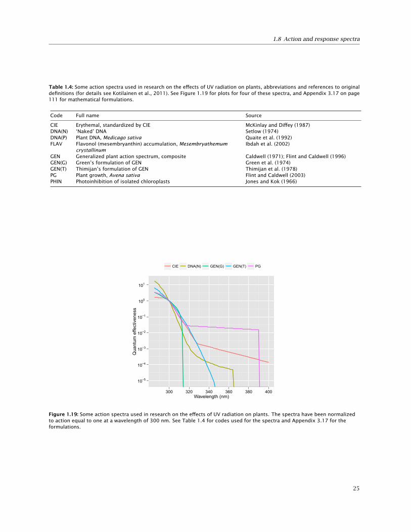
1.8 Action and response spectra

Table 1.4: Some action spectra used in research on the effects of UV radiation on plants, abbreviations and references to originaldefinitions (for details see Kotilainen et al., 2011). See Figure 1.19 for plots for four of these spectra, and Appendix 3.17 on page111 for mathematical formulations.

Code Full name Source

CIE Erythemal, standardized by CIE McKinlay and Diffey (1987)DNA(N) ‘Naked’ DNA Setlow (1974)DNA(P) Plant DNA, Medicago sativa Quaite et al. (1992)FLAV Flavonol (mesembryanthin) accumulation, Mesembryathemum

crystallinumIbdah et al. (2002)

GEN Generalized plant action spectrum, composite Caldwell (1971); Flint and Caldwell (1996)GEN(G) Green’s formulation of GEN Green et al. (1974)GEN(T) Thimijan’s formulation of GEN Thimijan et al. (1978)PG Plant growth, Avena sativa Flint and Caldwell (2003)PHIN Photoinhibition of isolated chloroplasts Jones and Kok (1966)

10−5

10−4

10−3

10−2

10−1

100

101

300 320 340 360 380 400Wavelength (nm)

Qua

ntum

effe

ctiv

enes

s

CIE DNA(N) GEN(G) GEN(T) PG

Figure 1.19: Some action spectra used in research on the effects of UV radiation on plants. The spectra have been normalizedto action equal to one at a wavelength of 300 nm. See Table 1.4 for codes used for the spectra and Appendix 3.17 for theformulations.

25

1 Introduction

10−2

100

102

300 400Wavelength (nm)

Spe

ctra

l irr

adia

nce

(mW

m−2

nm

−1)

Sanalux WG295 WG305 WG320 WG335 WG360

Figure 1.20: Spectra of the different UV scenarios used in an experiment. Numbers refer to the UV cut-off position (50 % trans-mission) produced by different Schott coloured glass filters (thickness 3 mm, Schott, Mainz, Germany): WG295, WG305, WG320,WG335, and WG360 in combination with a layer of Sanalux glass (thickness 4 mm, Schott).

example of a quantifiable effect would be change in theobserved concentrations of flavonols.

1.8.2.1 The mathematics behind polychromaticaction spectra

The average proportionality s between differences in thebiological effective response of successive treatmentsi, ∆Wbe,i, and differences in exposure (fluence rate mul-tiplied by exposure time), ∆Hi is given by an averagequantity

si =∆Wbe,i∆Hi

(1.26)

All the values of si together are represented in the actionspectrum. If the wavebands of each treatment are smallenough, an action spectrum s(λ) can be expressed by amathematical function. Different functions are discussed(Cullen and Neale, 1997; Rundel, 1983). In the simplestcase the factors si are positive and decrease exponentiallywith increasing wavelength. Thus, one common form ofs(λ) is

s(λ) = e−k(λ−λ0) (1.27)

where k is a parameter, which has to be obtained for eachdifferent biological effect using a fitting procedure, and awavelength λ0, where the action spectra are normalisedto unity, e.g. λ0 = 300 nm. Other functions including apolynomial dependence on λ are also possible and per-haps necessary for describing complex mechanisms.

For the interpretation of the experimental data, the bio-logical effective response Wbe, it is necessary to consider

the wavelength dependency. Thus, it is crucial that theentire spectral irradiance E(λ, t) during the experiment isknown. Broad-band meters are not suitable in most cases.This dependency is included in the biological effectivedose function (exposure) Hbe, given by

Hbe =∫λ

∫ts(λ) · E(λ, t) dt dλ

=∫λs(λ) ·H(λ) dλ (1.28)

A mathematical model can separate wavelength and dosedependency for a set of experimental data by the use ofmathematical functions describing Wbe(Hbe) and optim-isation procedures, e.g. non-linear curve fitting (Cullenand Neale, 1997; Ghetti et al., 1999; Götz et al., 2010;Ibdah et al., 2002). The model assumes that photons atdifferent wavelengths act independently, but with dif-ferent quantum efficiency at the same absorption site,and therefore with the same mechanism. Regarding theshape and saturation of the observed UV effect, differentfunctions can describe the data of Wbe(Hbe), for examplea linear, hyperbolic or sigmoid function. A simple linearrelation is

Wbe(Hbe) = W0 ·Hbe (1.29)

with the parameter W0, which has to be determined bythe fitting procedure. If for example the exposure time ofthe UV radiation is constant and, therefore, not depend-ing on the duration of the experiment t, the combination

26

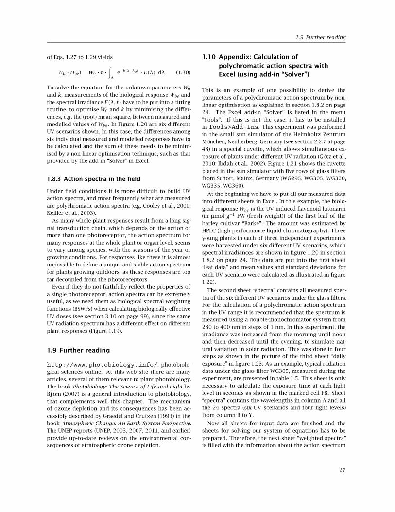
1.9 Further reading

of Eqs. 1.27 to 1.29 yields

Wbe(Hbe) = W0 · t ·∫λ

e−k(λ−λ0) · E(λ) dλ (1.30)

To solve the equation for the unknown parameters W0

and k, measurements of the biological response Wbe andthe spectral irradiance E(λ, t) have to be put into a fittingroutine, to optimise W0 and k by minimising the differ-ences, e.g. the (root) mean square, between measured andmodelled values of Wbe. In Figure 1.20 are six differentUV scenarios shown. In this case, the differences amongsix individual measured and modelled responses have tobe calculated and the sum of these needs to be minim-ised by a non-linear optimisation technique, such as thatprovided by the add-in “Solver" in Excel.

1.8.3 Action spectra in the field

Under field conditions it is more difficult to build UVaction spectra, and most frequently what are measuredare polychromatic action spectra (e.g. Cooley et al., 2000;Keiller et al., 2003).

As many whole-plant responses result from a long sig-nal transduction chain, which depends on the action ofmore than one photoreceptor, the action spectrum formany responses at the whole-plant or organ level, seemsto vary among species, with the seasons of the year orgrowing conditions. For responses like these it is almostimpossible to define a unique and stable action spectrumfor plants growing outdoors, as these responses are toofar decoupled from the photoreceptors.

Even if they do not faithfully reflect the properties ofa single photoreceptor, action spectra can be extremelyuseful, as we need them as biological spectral weightingfunctions (BSWFs) when calculating biologically effectiveUV doses (see section 3.10 on page 99), since the sameUV radiation spectrum has a different effect on differentplant responses (Figure 1.19).

1.9 Further reading

http://www.photobiology.info/, photobiolo-gical sciences online. At this web site there are manyarticles, several of them relevant to plant photobiology.The book Photobiology: The Science of Life and Light byBjörn (2007) is a general introduction to photobiology,that complements well this chapter. The mechanismof ozone depletion and its consequences has been ac-cessibly described by Graedel and Crutzen (1993) in thebook Atmospheric Change: An Earth System Perspective.The UNEP reports (UNEP, 2003, 2007, 2011, and earlier)provide up-to-date reviews on the environmental con-sequences of stratospheric ozone depletion.

1.10 Appendix: Calculation ofpolychromatic action spectra withExcel (using add-in “Solver”)

This is an example of one possibility to derive theparameters of a polychromatic action spectrum by non-linear optimisation as explained in section 1.8.2 on page24. The Excel add-in “Solver” is listed in the menu“Tools”. If this is not the case, it has to be installedin Tools>Add-Ins. This experiment was performedin the small sun simulator of the Helmholtz ZentrumMünchen, Neuherberg, Germany (see section 2.2.7 at page48) in a special cuvette, which allows simultaneous ex-posure of plants under different UV radiation (Götz et al.,2010; Ibdah et al., 2002). Figure 1.21 shows the cuvetteplaced in the sun simulator with five rows of glass filtersfrom Schott, Mainz, Germany (WG295, WG305, WG320,WG335, WG360).

At the beginning we have to put all our measured datainto different sheets in Excel. In this example, the biolo-gical response Wbe is the UV-induced flavonoid lutonarin(in µmol g−1 FW (fresh weight)) of the first leaf of thebarley cultivar “Barke”. The amount was estimated byHPLC (high performance liquid chromatography). Threeyoung plants in each of three independent experimentswere harvested under six different UV scenarios, whichspectral irradiances are shown in figure 1.20 in section1.8.2 on page 24. The data are put into the first sheet“leaf data” and mean values and standard deviations foreach UV scenario were calculated as illustrated in figure1.22).

The second sheet “spectra” contains all measured spec-tra of the six different UV scenarios under the glass filters.For the calculation of a polychromatic action spectrumin the UV range it is recommended that the spectrum ismeasured using a double-monochromator system from280 to 400 nm in steps of 1 nm. In this experiment, theirradiance was increased from the morning until noonand then decreased until the evening, to simulate nat-ural variation in solar radiation. This was done in foursteps as shown in the picture of the third sheet “dailyexposure” in figure 1.23. As an example, typical radiationdata under the glass filter WG305, measured during theexperiment, are presented in table 1.5. This sheet is onlynecessary to calculate the exposure time at each lightlevel in seconds as shown in the marked cell F8. Sheet“spectra” contains the wavelengths in column A and allthe 24 spectra (six UV scenarios and four light levels)from column B to Y.

Now all sheets for input data are finished and thesheets for solving our system of equations has to beprepared. Therefore, the next sheet “weighted spectra”is filled with the information about the action spectrum

27

1 Introduction

Figure 1.21: Special cuvette in the small sun simulator of the Helmholtz Zentrum München (see section 2.2.7 at page 48) coveredby five coloured glass filter from Schott, Mainz, Germany, to simulate five different UV scenarios. The filters from top to bot-tom are WG295, WG305, WG320, WG335 as well as WG360. The resulting spectral irradiances in the UV range for one specificincoming radiation is shown in figure 1.20 in section 1.8.2 on page 24. Photograph: Andreas Albert.

Table 1.5: PAR and UV radiation during the experiment for barley under the coloured glass filter WG305 (Schott, Mainz, Germany).

Light level 1 2 3 4 Unit

EUV-B 0.152 0.584 1.135 1.531 W m−2

EUV-A 8.76 19.78 24.67 38.74 W m−2

EPAR 114 228 256 363 W m−2

PPFD or QPAR 537 1073 1198 1692 µmol m−2 s−1

function as shown in figure 1.24. This sheet contains thecalculation of the biological effective dose function Hbeas presented in equation 1.28 on page 26. First, for theaction spectrum s(λ) an exponential function in chosen,as explained for equation 1.27 on page 26. Column A in-cludes the wavelengths and column B the estimated valueof the action spectrum using the parameter λ0 = 300 nmof cell B4 and k = 0.200 nm−1 of cell B5 (marked redin figure 1.24). This cell is only a link to cell B11 in thenext sheet “SOLVER”. Because it is only the starting valueof the optimisation procedure, the values of column Bdo not represent the real action spectrum. These valueswill change during optimisation. Below row 6, column Dand the following columns (in this case to column AA)include the values of the action spectrum of column Bmultiplied by the spectral irradiances of each UV scen-ario and light levels of sheet “spectra”. Row 1 and 2include the estimation of the UV doses. The cells in row

2 from column D and the following columns representthe integration over the wavelengths from 280 to 400 nmof each column beneath multiplied by the exposure timeof the respective UV scenario and light level as previouslycalculated in the sheet “daily exposure”. Integration inExcel is done by adding the values of the cells regardingthe wavelength step as shown for the marked cell D2 infigure 1.24. Here it is 1 nm. To get doses in units of Wsm−2 (J m−2), the sum is divided by a factor of 1000 be-cause the spectral irradiances were measured in mW m−2

nm−1. The daily UV dose (in kJ m−2) is then calculated inrow 1 for each UV scenario by adding the four values ofthe light levels. These daily UV doses are now needed forfurther calculations in the next sheet “SOLVER”.

The sheet “SOLVER” as illustrated in figure 1.25 in-cludes the comparison of the measured and modelleddata—as table and figure. The first five rows are a shortexplanation of the entire model. Especially row 5 con-

28

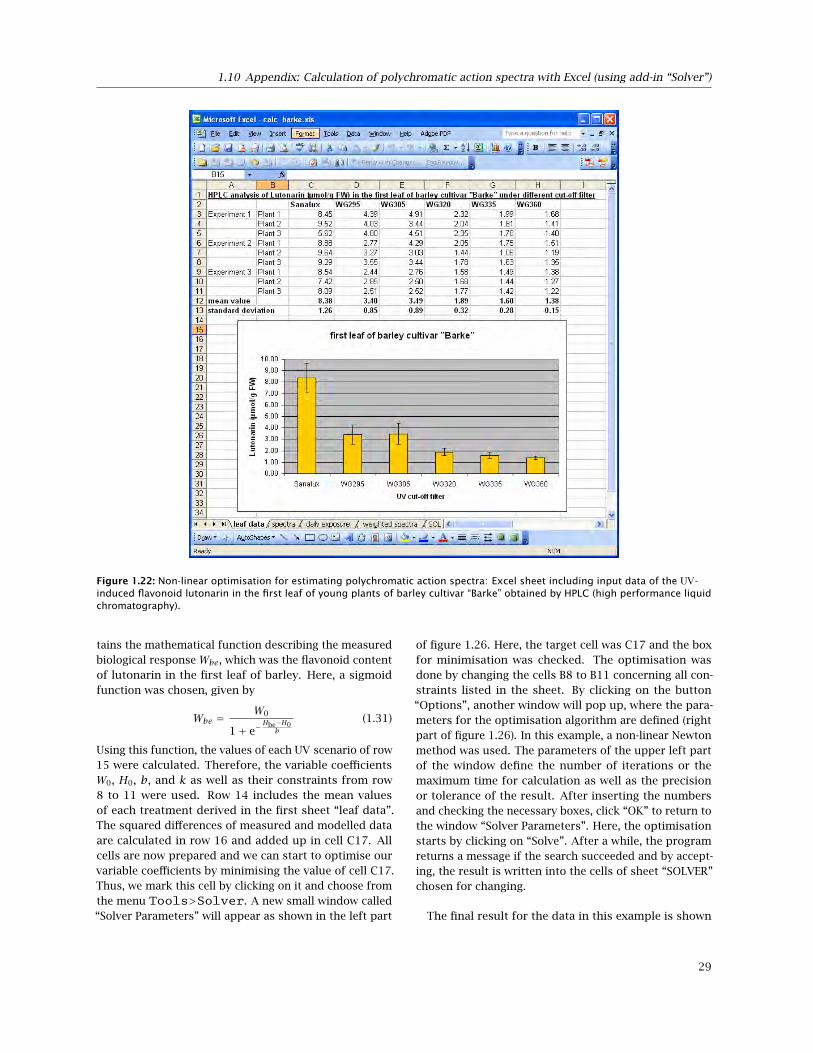
1.10 Appendix: Calculation of polychromatic action spectra with Excel (using add-in “Solver”)

Figure 1.22: Non-linear optimisation for estimating polychromatic action spectra: Excel sheet including input data of the UV-induced flavonoid lutonarin in the first leaf of young plants of barley cultivar “Barke” obtained by HPLC (high performance liquidchromatography).

tains the mathematical function describing the measuredbiological response Wbe, which was the flavonoid contentof lutonarin in the first leaf of barley. Here, a sigmoidfunction was chosen, given by

Wbe =W0

1+ e−Hbe−H0

b

(1.31)

Using this function, the values of each UV scenario of row15 were calculated. Therefore, the variable coefficientsW0, H0, b, and k as well as their constraints from row8 to 11 were used. Row 14 includes the mean valuesof each treatment derived in the first sheet “leaf data”.The squared differences of measured and modelled dataare calculated in row 16 and added up in cell C17. Allcells are now prepared and we can start to optimise ourvariable coefficients by minimising the value of cell C17.Thus, we mark this cell by clicking on it and choose fromthe menu Tools>Solver. A new small window called“Solver Parameters” will appear as shown in the left part

of figure 1.26. Here, the target cell was C17 and the boxfor minimisation was checked. The optimisation wasdone by changing the cells B8 to B11 concerning all con-straints listed in the sheet. By clicking on the button“Options”, another window will pop up, where the para-meters for the optimisation algorithm are defined (rightpart of figure 1.26). In this example, a non-linear Newtonmethod was used. The parameters of the upper left partof the window define the number of iterations or themaximum time for calculation as well as the precisionor tolerance of the result. After inserting the numbersand checking the necessary boxes, click “OK” to return tothe window “Solver Parameters”. Here, the optimisationstarts by clicking on “Solve”. After a while, the programreturns a message if the search succeeded and by accept-ing, the result is written into the cells of sheet “SOLVER”chosen for changing.

The final result for the data in this example is shown

29

1 Introduction

Figure 1.23: Non-linear optimisation for estimating polychromatic action spectra: Excel sheet including the information about thedaily variation of light levels and the derivation of exposure time of each light level.

in figure 1.27. The sum of the squared differences wasminimised to 0.13. The left graph in the bottom of figure1.27 shows two bars for each UV scenario, one for themeasured leaf data of row 14 (yellow) and the other onefor the modelled data of row 15 (purple). The result lookspromising. The most important parameter regarding theaction spectrum is k = 0.126 nm−1 in cell B11. This valuewas used to plot the actual action spectrum of this studyin the upper right graph of figure 1.27. Our action spec-trum is valid for wavelengths between 280 and 400 nm,

that interval which was chosen for integration in sheet“weighted spectra”.

This example describes just one possibility to solvea multi-variable and non-linear problem. For example,there is also a plugin available for Calc in OpenOf-fice.org. Therefore, if using Calc instead of Excel, thefile NLPSolver.oxt13 has to be installed by the exten-sion manager. Other search algorithms are used in thistool, but the result will be the same.

13available from http://extensions.services.openoffice.org/project/NLPSolver.

30

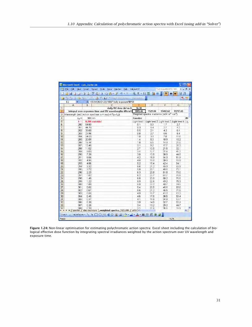
1.10 Appendix: Calculation of polychromatic action spectra with Excel (using add-in “Solver”)

Figure 1.24: Non-linear optimisation for estimating polychromatic action spectra: Excel sheet including the calculation of bio-logical effective dose function by integrating spectral irradiances weighted by the action spectrum over UV wavelength andexposure time.

31

1 Introduction

Figure 1.25: Non-linear optimisation for estimating polychromatic action spectra: Excel sheet with starting values of all variablecoefficients for the model, as table and graph, and the sum of squared differences between modelled and measured flavonoidcontent of lutonarin, which has to be minimised. The right graph at the bottom includes the actual action spectrum of this studycompared to other action spectra from the literature.

Figure 1.26: Popup windows for defining parameters (left) and options (right) in the Excel add-in “Solver”.

32

1.10 Appendix: Calculation of polychromatic action spectra with Excel (using add-in “Solver”)

Figure 1.27: Non-linear optimisation for estimating polychromatic action spectra: excel sheet with the results for all variablecoefficients after running the search algorithm.

33

2 Manipulating UV radiation

Pedro J. Aphalo, Andreas Albert, Andy McLeod, Anu Heikkilä, Iván Gómez, Félix López Figueroa, T. Matthew Robson,Åke Strid

2.1 Safety considerations

2.1.1 Risks related to sunlight exposure

When working in field experiments, workers and research-ers are exposed to sunlight as in any other outdoor activ-ity. To avoid health hazards adequate protection shouldbe used, either in the form of clothing or sun-blockinglotions. In some cases, for example when there is strongreflection of UV radiation by water, sand or snow-coveredsurfaces, eye protection in the form of sunglasses orgoggles should be used.

A common and simple parameter of the UV radiationlevel outdoors is the UV index, which was developedby the World Health Organization (WHO) including re-commended protection (WHO, 2002). The UV index isused for example in weather forecasts in integer num-bers from 1 to 11+, representing the UV exposure fromlow to extreme. 1

2.1.2 Risks related to the use of UV lamps

Lamps emitting UV-B and UV-C create a higher risk ofeye damage than sunlight because when UV radiation isnot accompanied by strong visible light the eye pupilsremain wide open. Also many lamps emit UV-C, whichis not present in sunlight at ground level and is moredamaging than UV-B. It is important to use goggles toprotect the eyes not only from UV radiation from thefront but also from the sides of the face. It is importantto ensure that the goggles used are designed to protectfrom UV radiation, rather than just from the impact offlying particles. The skin should also be well protected,

because in the same way as for plants, the effect of UV-Bon humans is enhanced under low visible light irradianceby the low rate of photoreactivation (light-driven repairof DNA damage).

Locations where UV lamps are in use should have vis-ibly located warning signs. Although there is no standard-ized symbol for UV radiation hazard, the warning symbolfor optical radiation (Figure 2.1) accompanied by the text‘UV radiation’ can be used. Additional text, ‘protect eyesand skin’ or ‘do not look directly at light source’ can beadded. Access to outdoor experiments should be restric-ted by fences with locked gates, and by locking accessdoors to greenhouses, controlled environment rooms andcabinets. This is to prevent exposure of people who areunaware of the risks involved. Everybody with access tothe area should be informed of risks, and trained to usethe protection and work procedures required to mitigatethem.

Lamps also pose risks unrelated to UV radiation. Fluor-escent tubes contain mercury and should disposed of ashazardous waste. The glass envelope of lamps is fragile,and can cause injuries if it breaks. Xenon-arc lamps alsopresent a relatively high risk of explosion, goggles andother face and body protection should be used. This riskis caused by the high pressure inside this type of lampand is present irrespective of the xenon-arc lamps beingon or off.

Lasers, can easily produce injuries, and should behandled with great care. Even the very low power laserpointers used during lectures are capable of injuring theeye if pointed towards the audience. As with UV lightsources, access to any type of laser should be restrictedto trained users, and eye protection should be worn to

1The UV index IUV is based on the spectral solar irradiance E(λ) and is related to the erythemal effective irradiance ECIE. The value is calculatedusing the constant factor ker = 40 m2 W−1 and the CIE erythemal action spectrum sCIE(λ) of equation 3.11 at page 112:

IUV = ker ·∫ 400 nm

250 nmE(λ) sCIE(λ) dλ

35

2 Manipulating UV radiation

Figure 2.1: From left to right: warning sign for optical radiation, warning sign for electricity, mandatory action sign for eye pro-tection, mandatory action sign for keep locked. At http://en.wikipedia.org/wiki/User:DrTorstenHenning/imagegallery these and other signs according to DIN standard 4844-2 are available both as vector graphics and bitmaps.These images are in the public domain.

match the wavelength emitted by each particular laser.Recommendations relating to warning signs, given above,apply equally to lasers and UV lamps.

2.1.3 Risks related to electrical power

Using mains power for either instruments or lamps, in-volves a risk of electric shock and this is especially truein humid conditions and outdoors. All components, likeconnectors, enclosures, and switches, should have an IPrating2 and any other codes required for their use in aparticular environment. When using mains power in aroom where there is water, it is usually a requirementto have grounded mains sockets protected with residualcurrent devices (RCD). These sense the current imbalancein the power line caused by a current leak to ground, forexample caused by the accidental flow of current throughthe body of an operator. When this residual current issensed, the device trips and disconnects power in a fewmilliseconds so preventing serious injury. RCDs andearth grounding should be regularly tested. Never usean electrical device that has a grounded plug in a mainssocket lacking ground contacts because this will createa risk of electrocution and in addition may negativelyaffect the functioning of measuring instruments.

2.1.4 Safety regulations and recommendations

The EU directive 2006/25/EC about protectingworkers from optical radiation can be found athttp://eur-lex.europa.eu/LexUriServ/LexUriServ.do?uri=OJ:L:2006:114:0038:0059:EN:PDF. This directive does not apply tosolar radiation. It gives maximum allowed levelsof exposure from artificial optical radiation sourcesand other requirements on how to achieve these and

the monitoring of workers health. Britain’s Healthand Safety Executive (HSE) has produced a guideon how to apply this directive (not approved yet byEU), that can be found at http://www.hse.gov.uk/radiation/nonionising/optical.htm.At this address, there is also information on sunexposure indicating that ‘UV radiation should beconsidered an occupational hazard for people whowork outdoors’. The World Health Organization (WHO)has issued general recommendations about protec-tion from the sun, which can be found at http://www.who.int/uv/sun_protection/en/.

2.2 Artificial sources of UV radiation

2.2.1 Lamps

2.2.1.1 Fluorescent lamps and tubes

Fluorescent lamps and tubes are low pressure mercuryvapour lamps. The mercury vapour emits radiation atspecific spectral lines, mostly in the UV region of thespectrum. Except for the case of germicidal UV-C lampsthe inside of the glass tube is coated with a layer of‘phosphor’3 which absorbs UV radiation and re-emits theenergy as fluorescence, at longer wavelengths, either asUV-B, UV-A, or visible radiation. There are even somefluorescent tubes producing far-red radiation around 750nm. For environmental UV studies we are interested inUV-B and UV-A emitting lamps. These lamps emit acrossa rather broad wavelength band, and have several minorsecondary peaks in the UV-C and visible regions. Figure2.2 shows the emission spectra of some UV lamps.

It should be remembered when designing experimentsthat UV-B lamps should be always filtered with cellulosediacetate film or some other material to remove UV-C,otherwise the effects observed will not be only due to

2IP stands for ‘ingress protection’ and usual codes are composed of the letters ‘IP’ and two digits. The first digit indicates level of protection forsolids and the second digit level of protection for water. For example IP20 indicates protection from ingress of fingers, and no protection fromwater; IP54 means dust and splashing water protected; IP65 means dust tight and protected from water jets; IP67 adds protection to immersionin water to up to 1 m depth.

3Different phosphorous chemical compounds which fluoresce at different wavelengths, or their mixtures, are used in fluorescent lamps to produceradiation of different wavelengths. These phosphorous compounds are called ‘phosphors’ in the lamp industry.

36

2.2 Artificial sources of UV radiation

Q−Panel UVA340

Q−Panel UVB313

Philips TL12

0.00

0.01

0.02

0.03

0.04

0.00

0.01

0.02

0.03

0.04

0.00

0.01

0.02

0.03

0.04

300 400 500 600 700 800Wavelength (nm)

Spe

ctra

l irra

dian

ce (r

elat

ive

ener

gy u

nits

)

Figure 2.2: Emission spectra of unfiltered Q-Panel UVA-340, Q-Panel UVB-313 and Philips TL40/12 lamps. Spectral energy irradi-ance relative to total area under each curve. Measured with a Macam double monochromator scanning spectroradiometer.

UV-B but also to UV-C radiation. The emission of UV-Cradiation might look small in energy terms but, beingvery effective in eliciting biological effects, it is capableof completely distorting the apparent response of plantsand other organisms to UV-B radiation in an experiment.In the case of UV-A lamps, both UV-B and UV-C radiationshould be removed by filtration.

Ultraviolet emitting fluorescent lamps also emit a smallamount of visible radiation, even in the red and orangeregions of the spectrum. This should not be forgottenwhen using these lamps as the only source of radiation.For example the very small amount of red-orange lightcan be enough to enhance germination of silver birchseeds in Petri dishes when irradiated with UV-B lamps(Pedro J. Aphalo, unpublished data).

The most commonly used UV-B and UV-A lamps are1200 mm-long tubes, rated at 40 W of electrical power.These lamps are sold for materials testing (Q-Panel UVB-313 and UVB-340, Q-Labs Inc., Farnworth, England) andfor medical use (Philips TL-40 W12, and TL-40 W 01,Philips, Amsterdam, The Netherlands). The second ofthese lamp types from Philips emits UV-B over a verynarrow peak, and are not suited for simulating ozonedepletion, but might be useful when the aim is not tosimulate solar radiation. There are also other lamp typesavailable, for example small-sized compact fluorescent

lamps such as PL-S 9W 01 from Philips.

Using fluorescent lamps requires some additionalequipment (Figure 2.3). The main component is a “ballast”which limits the current through the lamp. Traditionalballasts are electromagnetic, comprising a coil woundon a ferrous core, and require one more component, a‘starter’ for turning on the lamps. Lamps driven by suchballasts run at power-line frequency, 50 Hz in Europeand 60 Hz in USA, causing UV emission to flicker in time.This flicker is not visible to humans, but is visible tosome insects. The modern alternatives are electronicballasts driving the lamps at high frequency (in the or-der of 50–100 kHz) which together with the latency ofthe phosphor yields an almost constant radiation outputfrom the lamps. Consequently, we recommend the useof high frequency ballasts to avoid artifacts. Electronicballasts do not require starters.

Some types of electronic ballasts are dimming bal-lasts, allowing the adjustment of lamp output from fullpower down to a ballast-type-specific low value, usuallysomewhere between 1 and 10% of full power. Dimmingof lamp output can also be achieved using electromag-netic ballasts and phase-angle dimming controllers butthese enhance the visible flicker of the lamps. Someballasts are designed for newer T8 (thin, 26 mm dia-meter) tubes rather than the old-fashioned T12 (thick,

37

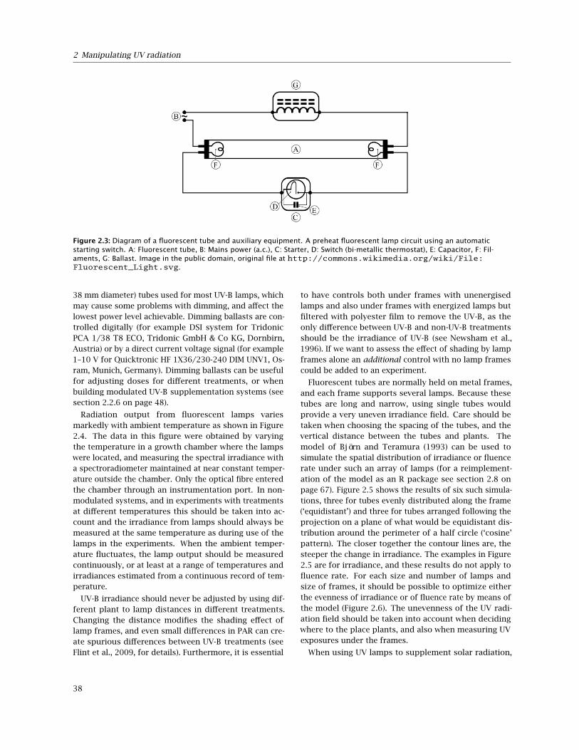
2 Manipulating UV radiation

Figure 2.3: Diagram of a fluorescent tube and auxiliary equipment. A preheat fluorescent lamp circuit using an automaticstarting switch. A: Fluorescent tube, B: Mains power (a.c.), C: Starter, D: Switch (bi-metallic thermostat), E: Capacitor, F: Fil-aments, G: Ballast. Image in the public domain, original file at http://commons.wikimedia.org/wiki/File:Fluorescent_Light.svg.

38 mm diameter) tubes used for most UV-B lamps, whichmay cause some problems with dimming, and affect thelowest power level achievable. Dimming ballasts are con-trolled digitally (for example DSI system for TridonicPCA 1/38 T8 ECO, Tridonic GmbH & Co KG, Dornbirn,Austria) or by a direct current voltage signal (for example1–10 V for Quicktronic HF 1X36/230-240 DIM UNV1, Os-ram, Munich, Germany). Dimming ballasts can be usefulfor adjusting doses for different treatments, or whenbuilding modulated UV-B supplementation systems (seesection 2.2.6 on page 48).

Radiation output from fluorescent lamps variesmarkedly with ambient temperature as shown in Figure2.4. The data in this figure were obtained by varyingthe temperature in a growth chamber where the lampswere located, and measuring the spectral irradiance witha spectroradiometer maintained at near constant temper-ature outside the chamber. Only the optical fibre enteredthe chamber through an instrumentation port. In non-modulated systems, and in experiments with treatmentsat different temperatures this should be taken into ac-count and the irradiance from lamps should always bemeasured at the same temperature as during use of thelamps in the experiments. When the ambient temper-ature fluctuates, the lamp output should be measuredcontinuously, or at least at a range of temperatures andirradiances estimated from a continuous record of tem-perature.

UV-B irradiance should never be adjusted by using dif-ferent plant to lamp distances in different treatments.Changing the distance modifies the shading effect oflamp frames, and even small differences in PAR can cre-ate spurious differences between UV-B treatments (seeFlint et al., 2009, for details). Furthermore, it is essential

to have controls both under frames with unenergisedlamps and also under frames with energized lamps butfiltered with polyester film to remove the UV-B, as theonly difference between UV-B and non-UV-B treatmentsshould be the irradiance of UV-B (see Newsham et al.,1996). If we want to assess the effect of shading by lampframes alone an additional control with no lamp framescould be added to an experiment.

Fluorescent tubes are normally held on metal frames,and each frame supports several lamps. Because thesetubes are long and narrow, using single tubes wouldprovide a very uneven irradiance field. Care should betaken when choosing the spacing of the tubes, and thevertical distance between the tubes and plants. Themodel of Björn and Teramura (1993) can be used tosimulate the spatial distribution of irradiance or fluencerate under such an array of lamps (for a reimplement-ation of the model as an R package see section 2.8 onpage 67). Figure 2.5 shows the results of six such simula-tions, three for tubes evenly distributed along the frame(‘equidistant’) and three for tubes arranged following theprojection on a plane of what would be equidistant dis-tribution around the perimeter of a half circle (‘cosine’pattern). The closer together the contour lines are, thesteeper the change in irradiance. The examples in Figure2.5 are for irradiance, and these results do not apply tofluence rate. For each size and number of lamps andsize of frames, it should be possible to optimize eitherthe evenness of irradiance or of fluence rate by means ofthe model (Figure 2.6). The unevenness of the UV radi-ation field should be taken into account when decidingwhere to the place plants, and also when measuring UVexposures under the frames.

When using UV lamps to supplement solar radiation,

38

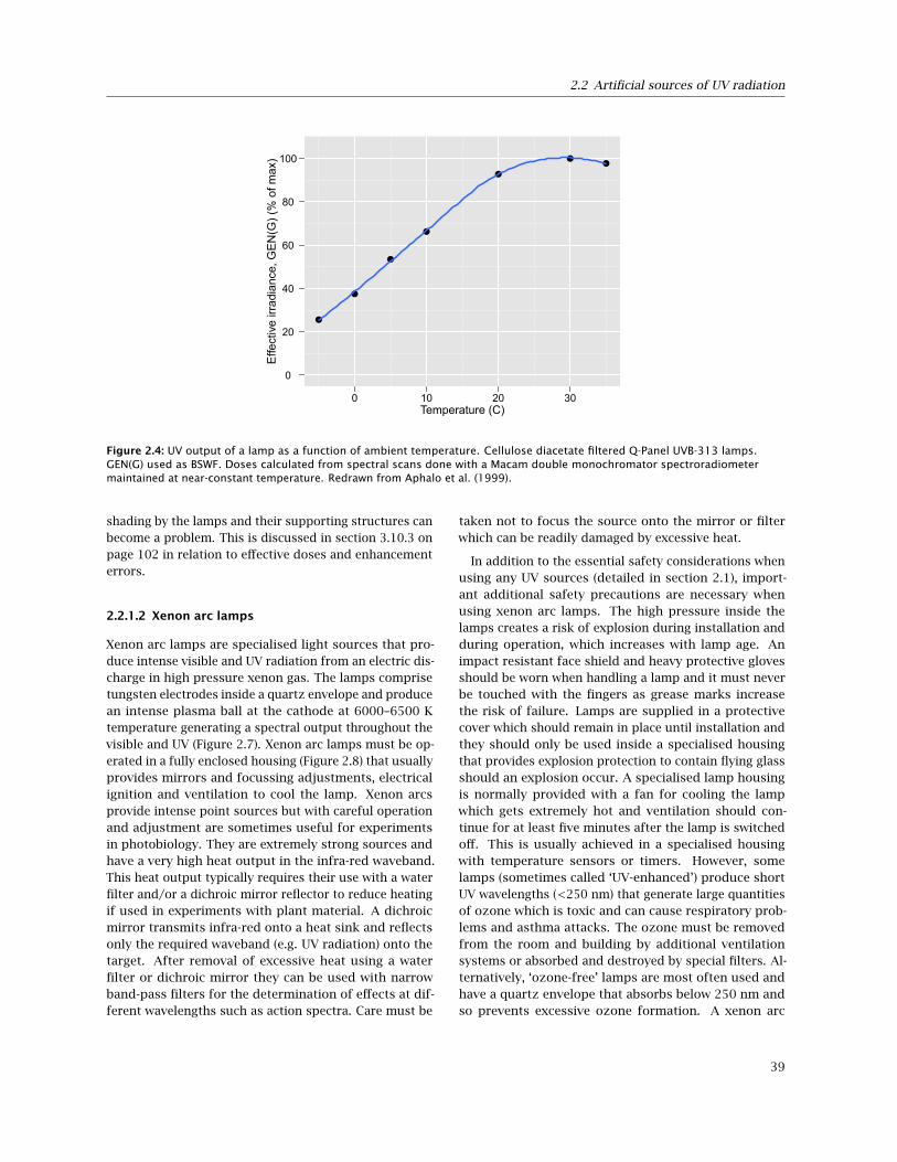
2.2 Artificial sources of UV radiation

0

20

40

60

80

100

0 10 20 30Temperature (C)

Effe

ctiv

e irr

adia

nce,

GE

N(G

) (%

of m

ax)

Figure 2.4: UV output of a lamp as a function of ambient temperature. Cellulose diacetate filtered Q-Panel UVB-313 lamps.GEN(G) used as BSWF. Doses calculated from spectral scans done with a Macam double monochromator spectroradiometermaintained at near-constant temperature. Redrawn from Aphalo et al. (1999).

shading by the lamps and their supporting structures canbecome a problem. This is discussed in section 3.10.3 onpage 102 in relation to effective doses and enhancementerrors.

2.2.1.2 Xenon arc lamps

Xenon arc lamps are specialised light sources that pro-duce intense visible and UV radiation from an electric dis-charge in high pressure xenon gas. The lamps comprisetungsten electrodes inside a quartz envelope and producean intense plasma ball at the cathode at 6000–6500 Ktemperature generating a spectral output throughout thevisible and UV (Figure 2.7). Xenon arc lamps must be op-erated in a fully enclosed housing (Figure 2.8) that usuallyprovides mirrors and focussing adjustments, electricalignition and ventilation to cool the lamp. Xenon arcsprovide intense point sources but with careful operationand adjustment are sometimes useful for experimentsin photobiology. They are extremely strong sources andhave a very high heat output in the infra-red waveband.This heat output typically requires their use with a waterfilter and/or a dichroic mirror reflector to reduce heatingif used in experiments with plant material. A dichroicmirror transmits infra-red onto a heat sink and reflectsonly the required waveband (e.g. UV radiation) onto thetarget. After removal of excessive heat using a waterfilter or dichroic mirror they can be used with narrowband-pass filters for the determination of effects at dif-ferent wavelengths such as action spectra. Care must be

taken not to focus the source onto the mirror or filterwhich can be readily damaged by excessive heat.

In addition to the essential safety considerations whenusing any UV sources (detailed in section 2.1), import-ant additional safety precautions are necessary whenusing xenon arc lamps. The high pressure inside thelamps creates a risk of explosion during installation andduring operation, which increases with lamp age. Animpact resistant face shield and heavy protective glovesshould be worn when handling a lamp and it must neverbe touched with the fingers as grease marks increasethe risk of failure. Lamps are supplied in a protectivecover which should remain in place until installation andthey should only be used inside a specialised housingthat provides explosion protection to contain flying glassshould an explosion occur. A specialised lamp housingis normally provided with a fan for cooling the lampwhich gets extremely hot and ventilation should con-tinue for at least five minutes after the lamp is switchedoff. This is usually achieved in a specialised housingwith temperature sensors or timers. However, somelamps (sometimes called ‘UV-enhanced’) produce shortUV wavelengths (<250 nm) that generate large quantitiesof ozone which is toxic and can cause respiratory prob-lems and asthma attacks. The ozone must be removedfrom the room and building by additional ventilationsystems or absorbed and destroyed by special filters. Al-ternatively, ‘ozone-free’ lamps are most often used andhave a quartz envelope that absorbs below 250 nm andso prevents excessive ozone formation. A xenon arc

39

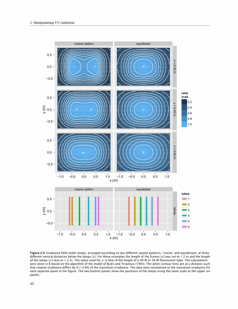
2 Manipulating UV radiation

'cosine' pattern equidistant

−0.5

0.0

0.5

−0.5

0.0

0.5

−0.5

0.0

0.5

z = 0.30 mz = 0.45 m

z = 0.60 m

−1.0 −0.5 0.0 0.5 1.0 −1.0 −0.5 0.0 0.5 1.0x (m)

y (m

)

relat.irrad.

0.2

0.4

0.6

0.8

1.0

'cosine' pattern equidistant

−0.5

0.0

0.5

lamps

−1.0 −0.5 0.0 0.5 1.0 −1.0 −0.5 0.0 0.5 1.0x (m)

y (m

)

tubes

1

2

3

4

5

6

Figure 2.5: Irradiance field under lamps, arranged according to two different spatial patterns, ‘cosine’ and equidistant, at threedifferent vertical distances below the lamps (z). For these examples the length of the frames (x) was set to 1.2 m and the lengthof the lamps (y) also to 1.2 m. The value used for y is that of the length of a 40 W or 36 W fluorescent tube. The calculationswere done in R based on the algorithm of the model of Björn and Teramura (1993). The white contour lines are at a distance suchthat relative irradiance differs by 0.1 (10%) of the maximum irradiance. The data were normalized to the maximum irradiance foreach separate panel in the figure. The two bottom panels show the positions of the lamps using the same scale as the upper sixpanels.

40

2.2 Artificial sources of UV radiation

fluence rate irradiance

−0.5

0.0

0.5

z = 0.40 m

−1.0 −0.5 0.0 0.5 1.0 −1.0 −0.5 0.0 0.5 1.0x (m)

y (m

)

relativeunits

0.2

0.4

0.6

0.8

1.0

−0.5

0.0

0.5

−1.0 −0.5 0.0 0.5 1.0x (m)

y (m

)

tubes

1

2

3

4

Figure 2.6: Irradiance and fluence rate fields under four lamps, arranged in a square, at a vertical distance below the lamps (z)of 0.40 m. For these examples the length of the frames (x) was set to 1.2 m and the length of the lamps (y) also to 1.2 m. Thevalue used for y is that of the length of a 40 W or 36 W fluorescent tube. The calculations were done in R based on the algorithmof the model of Björn and Teramura (1993). The white contour lines are at a distance such that relative irradiance or fluence ratediffers by 0.1 (10%) of the respective maximum. The bottom panel shows the positions of the lamps using the same scale as theupper two panels.

0.5

1.0

1.5

300 400 500 600 700Wavelength (nm)

Spe

ctra

l irr

adia

nce

( W m

−2 n

m−1

)

Figure 2.7: Spectral irradiance from a xenon arc source (Mueller Electonik-Optik, Germany) using an Osram 1000 W ‘ozone-free’lamp after filtration through a water infra-red filter.

41

2 Manipulating UV radiation

Figure 2.8: Xenon arc lamp (1000 watt, Mueller Elektronik-Optik, Germany) showing protective housing, high voltage power sup-ply, water filter, beam turner, filter holder and water cooled cuvette with quartz glass window (School of GeoSciences, Universityof Edinburgh, UK). Photograph: Andy R. McLeod.

lamp is extremely bright and the intense visible radiationcan damage the eyes in addition to UV effects. The arcor its intense image must never be viewed directly asit can cause permanent eye damage. When using theequipment, the illuminated areas may also be extremelybright and dark coloured goggles should be worn, suchas those used in welding that also provide UV protection,ensuring that the eyes are also protected from side il-lumination as well as directly. It is essential to followthe manufacturers’ instructions with respect to lamp lifeand operating current in order to maximise their usefullife and minimise the risk of failure due to explosion.Further information on xenon arc sources and other highintensity lamp sources sometimes used in photobiologyis provided by Holmes (1984).

2.2.2 Deuterium lamps

High intensity water-cooled deuterium lamps (150 W)have a fairly flat radiant intensity curve in the UV-B re-gion (approximately 1.5–3.0 mW m−2 nm−1 between 280and 300 nm at a distance of 30 cm) that is appropriate formechanistic plant UV photobiology studies. This type ofradiation sources (e.g. produced by Hamamatsu Photon-ics) requires a dedicated control box for operation but isstill an affordable alternative to lasers, starting at about2,500C for a setup. High intensity deuterium lamps havebeen used for wavelength dependence measurementsboth in photobiology (Kalbina et al., 2008; Kalbin et al.,2005) and photochemistry (Kalbin et al., 2005) when fit-ted with the appropriate filters. The lamp has to bemounted horizontally to allow efficient water cooling butusing spreading lenses and a mirror mounted in a 45

angle to the incident radiation a full Arabidopsis rosette

can easily be irradiated (Kalbina et al., 2008) and, the UVirradiation can be supplemented with PAR from externalsources as desired. A drawback of this type of equipmentis the short life of the radiation source (a few hundredhours). Spare lamps cost approximately 1 500 C.

2.2.3 LEDs

The principle of a light emitting diode (LED) is totallydifferent to conventional incandescent light bulbs. It isa semiconductor consisting of two types of layer: onelayer releasing electrons as a direct current to fill holes inanother. Energy is released as a photon at a wavelength(colour) that depends on the band gap energy of thematerials comprising each of the two layers (Figure 2.9).

Due to this emission of photons at a very precisewavelength, the typical spectrum of a LED shows onedistinct peak. The emitted wavelength range can be in-creased by adding a fluorescing material to the LED. Thisis shown in Figure 2.10 together with a measurement ofthe solar irradiance at the Helmholtz Zentrum Münchenin Neuherberg, Germany. The maximum spectral irradi-ance of the LED peak (measurement at 20 cm distance)is more than one order of magnitude lower than thatof the solar irradiance (which is the reason a semilogar-ithmic scale is used). All measurements were made usinga double-monochromator spectroradiometer (Bentham,Reading, UK).

If the correct semiconductor material is chosen, almostany wavelength can be produced even in the UV range.The intensity of UV LEDs (Figure 2.11) is much lowerthan that of LEDs emitting visible light, even at a shorterdistance than in Figure 2.10. Normally, the optical powerof a LED is around 1 W or less for visible radiation and

42

2.2 Artificial sources of UV radiation

Figure 2.9: Light emitting diode (LED) junction and the flow of electrons and holes. Diagram by s-Kei, under Creative Com-mons Attribution-Share Alike 2.5 Generic license, original at http://commons.wikimedia.org/wiki/File:PnJunction-LED-E.svg.

10−2

100

102

300 400 500 600 700 800Wavelength (nm)

Spe

ctra

l irr

adia

nce

(mW

m−2

nm

−1)

red LED sunlight at noon white LED

Figure 2.10: Emission spectra of a red and white LED measured at a 20 cm distance compared to an outdoor measurement at theHelmholtz Zentrum München, Neuherberg, Germany.

43

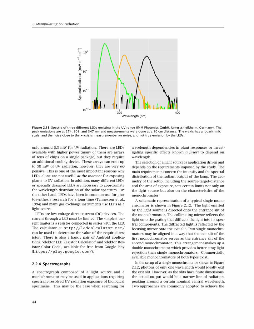
2 Manipulating UV radiation

10−3

10−2

10−1

100

300 400Wavelength (nm)

Spe

ctra

l irra

dian

ce (

mW

m−2

nm

−1)

Figure 2.11: Spectra of three different LEDs emitting in the UV range (IMM Photonics GmbH, Unterschleißheim, Germany). Thepeak emissions are at 274, 308, and 347 nm and measurements were done at a 10 cm distance. The y-axis has a logarithmicscale, and the noise close to the x-axis is measurement-error noise, and not true emission by the LEDs.

only around 0.5 mW for UV radiation. There are LEDsavailable with higher power (many of them are arraysof tens of chips on a single package) but they requirean additional cooling device. These arrays can emit upto 50 mW of UV radiation, however, they are very ex-pensive. This is one of the most important reasons whyLEDs alone are not useful at the moment for exposingplants to UV radiation. In addition, many different LEDsor specially designed LEDs are necessary to approximatethe wavelength distribution of the solar spectrum. Onthe other hand, LEDs have been in common use for pho-tosynthesis research for a long time (Tennessen et al.,1994) and many gas-exchange instruments use LEDs as alight source.

LEDs are low voltage direct current (DC) devices. Thecurrent through a LED must be limited. The simplest cur-rent limiter is a resistor connected in series with the LED.The calculator at http://ledcalculator.net/can be used to determine the value of the required res-istor. There is also a handy pair of Android applica-tions, ‘elektor LED Resistor Calculator’ and ‘elektor Res-istor Color Code’, available for free from Google Play(https://play.google.com/).

2.2.4 Spectrographs

A spectrograph composed of a light source and amonochromator may be used in applications requiringspectrally-resolved UV radiation exposure of biologicalspecimens. This may be the case when searching for

wavelength dependencies in plant responses or invest-igating specific effects known a priori to depend onwavelength.

The selection of a light source is application driven anddepends on the requirements imposed by the study. Themain requirements concern the intensity and the spectraldistribution of the radiant output of the lamp. The geo-metry of the setup, including the source-target-distanceand the area of exposure, sets certain limits not only onthe light source but also on the characteristics of themonochromator.

A schematic representation of a typical single mono-chromator is shown in Figure 2.12. The light emittedby the light source is directed onto the entrance slit ofthe monochromator. The collimating mirror reflects thelight onto the grating that diffracts the light into its spec-tral components. The diffracted light is reflected by thefocusing mirror onto the exit slit. Two single monochro-mators may be aligned in a way that the exit slit of thefirst monochromator serves as the entrance slit of thesecond monochromator. This arrangement makes up adouble monochromator which provides better stray lightrejection than single monochromators. Commerciallyavailable monochromators of both types exist.

In the setup of a single monochromator shown in Figure2.12, photons of only one wavelength would ideally exitthe exit slit. However, as the slits have finite dimensions,the actual output would be a narrow line of radiation,peaking around a certain nominal central wavelength.Two approaches are commonly adopted to achieve the

44

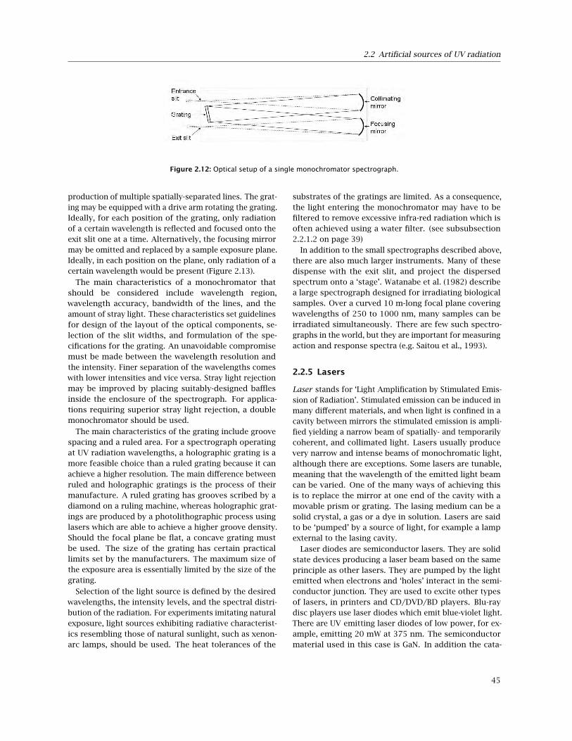
2.2 Artificial sources of UV radiation

Figure 2.12: Optical setup of a single monochromator spectrograph.

production of multiple spatially-separated lines. The grat-ing may be equipped with a drive arm rotating the grating.Ideally, for each position of the grating, only radiationof a certain wavelength is reflected and focused onto theexit slit one at a time. Alternatively, the focusing mirrormay be omitted and replaced by a sample exposure plane.Ideally, in each position on the plane, only radiation of acertain wavelength would be present (Figure 2.13).

The main characteristics of a monochromator thatshould be considered include wavelength region,wavelength accuracy, bandwidth of the lines, and theamount of stray light. These characteristics set guidelinesfor design of the layout of the optical components, se-lection of the slit widths, and formulation of the spe-cifications for the grating. An unavoidable compromisemust be made between the wavelength resolution andthe intensity. Finer separation of the wavelengths comeswith lower intensities and vice versa. Stray light rejectionmay be improved by placing suitably-designed bafflesinside the enclosure of the spectrograph. For applica-tions requiring superior stray light rejection, a doublemonochromator should be used.

The main characteristics of the grating include groovespacing and a ruled area. For a spectrograph operatingat UV radiation wavelengths, a holographic grating is amore feasible choice than a ruled grating because it canachieve a higher resolution. The main difference betweenruled and holographic gratings is the process of theirmanufacture. A ruled grating has grooves scribed by adiamond on a ruling machine, whereas holographic grat-ings are produced by a photolithographic process usinglasers which are able to achieve a higher groove density.Should the focal plane be flat, a concave grating mustbe used. The size of the grating has certain practicallimits set by the manufacturers. The maximum size ofthe exposure area is essentially limited by the size of thegrating.

Selection of the light source is defined by the desiredwavelengths, the intensity levels, and the spectral distri-bution of the radiation. For experiments imitating naturalexposure, light sources exhibiting radiative characterist-ics resembling those of natural sunlight, such as xenon-arc lamps, should be used. The heat tolerances of the

substrates of the gratings are limited. As a consequence,the light entering the monochromator may have to befiltered to remove excessive infra-red radiation which isoften achieved using a water filter. (see subsubsection2.2.1.2 on page 39)

In addition to the small spectrographs described above,there are also much larger instruments. Many of thesedispense with the exit slit, and project the dispersedspectrum onto a ‘stage’. Watanabe et al. (1982) describea large spectrograph designed for irradiating biologicalsamples. Over a curved 10 m-long focal plane coveringwavelengths of 250 to 1000 nm, many samples can beirradiated simultaneously. There are few such spectro-graphs in the world, but they are important for measuringaction and response spectra (e.g. Saitou et al., 1993).

2.2.5 Lasers

Laser stands for ‘Light Amplification by Stimulated Emis-sion of Radiation’. Stimulated emission can be induced inmany different materials, and when light is confined in acavity between mirrors the stimulated emission is ampli-fied yielding a narrow beam of spatially- and temporarilycoherent, and collimated light. Lasers usually producevery narrow and intense beams of monochromatic light,although there are exceptions. Some lasers are tunable,meaning that the wavelength of the emitted light beamcan be varied. One of the many ways of achieving thisis to replace the mirror at one end of the cavity with amovable prism or grating. The lasing medium can be asolid crystal, a gas or a dye in solution. Lasers are saidto be ‘pumped’ by a source of light, for example a lampexternal to the lasing cavity.

Laser diodes are semiconductor lasers. They are solidstate devices producing a laser beam based on the sameprinciple as other lasers. They are pumped by the lightemitted when electrons and ‘holes’ interact in the semi-conductor junction. They are used to excite other typesof lasers, in printers and CD/DVD/BD players. Blu-raydisc players use laser diodes which emit blue-violet light.There are UV emitting laser diodes of low power, for ex-ample, emitting 20 mW at 375 nm. The semiconductormaterial used in this case is GaN. In addition the cata-

45

2 Manipulating UV radiation

Figure 2.13: Spectrograph constructed to produce spectrally-resolved UV radiation for material degradation studies. (Cover opento show components. Photograph: Anu Heikkilä.)

logue of Roithner Lasertechnik GmbH (Vienna, Austria)lists ‘diode pumped solid state lasers’ emitting at 266 nmand at 355 nm. Non solid-state lasers that emit in the UVregion are also available. For example argon ion laserscontinuously emit at wavelengths of 334 and 351 nm.

The power of lasers varies from 1–5 mW for laser point-ers to 100 kW for lasers under development for militaryuse. The coherent and concentrated beam can cause seri-ous damage to eyesight, and safety precautions shouldbe taken during their use, unless they are of very lowpower (see section 2.1 on page 35).

Lasers can be used for example in characterizing theslit function of spectrometers (see section 3.7.2.2 on page93), for aligning optics, and in the ubiquitous barcodereaders used in supermarkets and laser pointers used byspeakers during lectures. They are used in instrumentslike confocal microscopes and different analytical pro-cedures in chemistry and biology. They can also be usedto excite photochemical or photobiological systems if thetarget is small.

For the purpose of UV photobiology, tunable op-tical parametric oscillator (OPO) pump lasers (pumpwavelength 355 nm) are especially useful in mechanisticstudies such as in accurate wavelength dependence de-terminations or action spectroscopy (O’Hara, Strid andJenkins, in preparation). Placing a cuvette holder in thebeam, a plant extract or a protein solution can be accur-ately irradiated using 50 or 100 µl cuvettes. By usingthe appropriate optics (lenses, mirrors, etc.; Figure 2.14),the geometry of the beam can be manipulated so that alarger area or sample (several cm2) can be illuminated.This is large enough for exposing for instance part of anArabidopsis rosette, or for simultaneously irradiating twodetached Arabidopsis leaves. Tuneable lasers can alsobe used for studies of complex mechanistic interactions

between several plant photoreceptors, since they can beused within a short time interval (seconds) at differentwavelengths, e.g. for irradiation first in the UV-B, then inthe blue or red.

When using lasers for photobiological purposes, a num-ber of circumstances need to be taken into account.Lasers emit their radiation in the form of pulses andthis should be kept in mind when designing the exper-iments. Usually, both the energy of the pulses and thepulse rate can be varied within limits, depending on thesophistication (and price!) of the equipment. Pulse ratesbetween 1 to 20 Hz in the more affordable machinesup to 1000 Hz in the more expensive ones can be ob-tained. The pulses are typically 5–10 ns in length and thelinewidth is usually around 0.5 nm (Figure 2.15), makingthis type of instrumentation ideal for studies of the initialUV signalling events on the biochemical and cell biolo-gical levels. Also, due to the physical principles on whicha tunable laser in the UV region relies, some residualradiation with double the desired wavelength may still bepresent in the beam exiting the apparatus. This has to betaken care of by using a filter in the light-path blockingthe longer wavelengths. For instance, when irradiating aplant with a wavelength of 300 nm, care must be takenso that any 600 nm component will be blocked out to besure that the biological effect is due to the UV-B aloneand not the red light. Of course, the laser UV-B radiationcan be supplemented with PAR from other light sourcesas required.

Laser radiation is measured as the energy emitted (in J)in each pulse or in a train of pulses using a pulse energymeter. This then has to be related to the area actuallyirradiated. The maximal output energy for a flash at280 nm typically ranges between 40 and 200 µJ. Thespectral bandwidth and the accuracy of the wavelength

46

2.2 Artificial sources of UV radiation

Figure 2.14: Set-up with an Opolette 355 II+UV tunable laser (a) for irradiation of plant extracts or a protein solution placedin a 50- or 100-µl cuvette in the Peltier-cooled cuvette holder (a–c). The Figures also show the attenuator, the cut-off filter (forremoving red light), the lens for achieving the desired geometry of the beam, and the laser pulse power sensor (a, b), that all arepresent in the light path, as well as the read-out unit for the power sensor (c). For exposure of plant leaves or a small pot contain-ing an Arabidopsis plant, the cuvette holder is removed and a mirror is placed at 45 angle where the power sensor is seen in (a).This mirror deflects the laser beam through a hole in the shelf hitting an area on the bench top where the leaves/plant are placed.Photographs: Åke Strid.

Figure 2.15: The sharp 300 nm peak from an Opolette 355II+UV (Opotek Inc, Carlsbad, CA) tunable laser with a halfbandwidth of0.4 nm as measured using a SM440 diode array spectroradiometer (Spectral Products, Putnam, CT). Representation on the Y-axisis in arbitrary units. Figure by Strid, Åke (2012) unpublished.

47

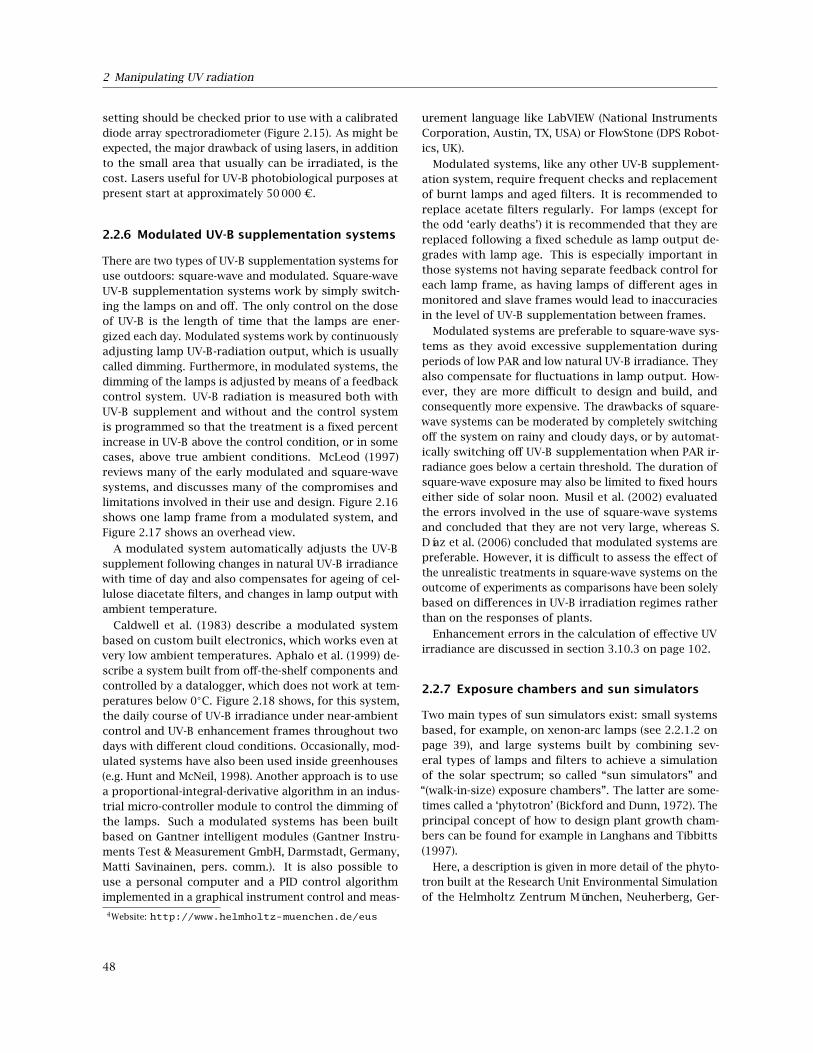
2 Manipulating UV radiation

setting should be checked prior to use with a calibrateddiode array spectroradiometer (Figure 2.15). As might beexpected, the major drawback of using lasers, in additionto the small area that usually can be irradiated, is thecost. Lasers useful for UV-B photobiological purposes atpresent start at approximately 50 000 C.

2.2.6 Modulated UV-B supplementation systems

There are two types of UV-B supplementation systems foruse outdoors: square-wave and modulated. Square-waveUV-B supplementation systems work by simply switch-ing the lamps on and off. The only control on the doseof UV-B is the length of time that the lamps are ener-gized each day. Modulated systems work by continuouslyadjusting lamp UV-B-radiation output, which is usuallycalled dimming. Furthermore, in modulated systems, thedimming of the lamps is adjusted by means of a feedbackcontrol system. UV-B radiation is measured both withUV-B supplement and without and the control systemis programmed so that the treatment is a fixed percentincrease in UV-B above the control condition, or in somecases, above true ambient conditions. McLeod (1997)reviews many of the early modulated and square-wavesystems, and discusses many of the compromises andlimitations involved in their use and design. Figure 2.16shows one lamp frame from a modulated system, andFigure 2.17 shows an overhead view.

A modulated system automatically adjusts the UV-Bsupplement following changes in natural UV-B irradiancewith time of day and also compensates for ageing of cel-lulose diacetate filters, and changes in lamp output withambient temperature.

Caldwell et al. (1983) describe a modulated systembased on custom built electronics, which works even atvery low ambient temperatures. Aphalo et al. (1999) de-scribe a system built from off-the-shelf components andcontrolled by a datalogger, which does not work at tem-peratures below 0C. Figure 2.18 shows, for this system,the daily course of UV-B irradiance under near-ambientcontrol and UV-B enhancement frames throughout twodays with different cloud conditions. Occasionally, mod-ulated systems have also been used inside greenhouses(e.g. Hunt and McNeil, 1998). Another approach is to usea proportional-integral-derivative algorithm in an indus-trial micro-controller module to control the dimming ofthe lamps. Such a modulated systems has been builtbased on Gantner intelligent modules (Gantner Instru-ments Test & Measurement GmbH, Darmstadt, Germany,Matti Savinainen, pers. comm.). It is also possible touse a personal computer and a PID control algorithmimplemented in a graphical instrument control and meas-

urement language like LabVIEW (National InstrumentsCorporation, Austin, TX, USA) or FlowStone (DPS Robot-ics, UK).

Modulated systems, like any other UV-B supplement-ation system, require frequent checks and replacementof burnt lamps and aged filters. It is recommended toreplace acetate filters regularly. For lamps (except forthe odd ‘early deaths’) it is recommended that they arereplaced following a fixed schedule as lamp output de-grades with lamp age. This is especially important inthose systems not having separate feedback control foreach lamp frame, as having lamps of different ages inmonitored and slave frames would lead to inaccuraciesin the level of UV-B supplementation between frames.

Modulated systems are preferable to square-wave sys-tems as they avoid excessive supplementation duringperiods of low PAR and low natural UV-B irradiance. Theyalso compensate for fluctuations in lamp output. How-ever, they are more difficult to design and build, andconsequently more expensive. The drawbacks of square-wave systems can be moderated by completely switchingoff the system on rainy and cloudy days, or by automat-ically switching off UV-B supplementation when PAR ir-radiance goes below a certain threshold. The duration ofsquare-wave exposure may also be limited to fixed hourseither side of solar noon. Musil et al. (2002) evaluatedthe errors involved in the use of square-wave systemsand concluded that they are not very large, whereas S.Díaz et al. (2006) concluded that modulated systems arepreferable. However, it is difficult to assess the effect ofthe unrealistic treatments in square-wave systems on theoutcome of experiments as comparisons have been solelybased on differences in UV-B irradiation regimes ratherthan on the responses of plants.

Enhancement errors in the calculation of effective UVirradiance are discussed in section 3.10.3 on page 102.

2.2.7 Exposure chambers and sun simulators

Two main types of sun simulators exist: small systemsbased, for example, on xenon-arc lamps (see 2.2.1.2 onpage 39), and large systems built by combining sev-eral types of lamps and filters to achieve a simulationof the solar spectrum; so called “sun simulators” and“(walk-in-size) exposure chambers”. The latter are some-times called a ‘phytotron’ (Bickford and Dunn, 1972). Theprincipal concept of how to design plant growth cham-bers can be found for example in Langhans and Tibbitts(1997).

Here, a description is given in more detail of the phyto-tron built at the Research Unit Environmental Simulationof the Helmholtz Zentrum München, Neuherberg, Ger-

4Website: http://www.helmholtz-muenchen.de/eus

48

2.2 Artificial sources of UV radiation

Figure 2.16: Modulated UV-B supplementation system in Joensuu in 1997. See Aphalo et al. (1999) for details. Photograph: PedroJ. Aphalo.

Figure 2.17: Modulated UV-B supplementation system in Joensuu in 2012. The new design of the support reduces shading.Infrared heating has been added along the middle of the frames. Photo: Matti Savinainen

49

2 Manipulating UV radiation

238 242

0

20

40

60

80

06:00 12:00 18:00 24:00 06:00 12:00 18:00 24:00Time of day

Mea

n e

ffect

ive

irra

dian

ce C

IE (

mW

m−2

)

Figure 2.18: UV-B irradiance under a modulated system on two days differing in cloud cover. Data for 30% enhanced UV-B treat-ment (dashed line) and UV-A control (solid line). Days 238 and 242 of year 1997, at Joensuu, Finland. UV irradiance measuredwith two matched Vital Technologies’ (Bolton, Ontario, Canada; no longer in business) ‘Blue Wave’ BW-20 erythemal sensors.From Aphalo et al. (1999).

many4. This phytotron facility consists of a set of sevenclosed chambers (length · width · height):

• four walk-in-size chambers (3.4 m × 2.8 m × 2.5 m),

• two medium-size sun simulators (1.4 m × 1.4 m ×1.0 m),

• one small sun simulator (1.2 m × 1.2 m × 0.4 m).

In order to extrapolate response of plants from experi-ments to those in their natural habitat, these experimentsneed to be performed under realistic and reproducibleconditions. The radiation provided must be as realisticas possible. Not only the quantity but also the spectralquality of radiation has to match the seasonal and diurnalvariations occurring in nature (Caldwell and Flint, 1994a).This includes the steep absorption characteristics of UVradiation that result from the filtering of solar irradianceby stratospheric ozone as well as the balance betweenthe UV-B, UV-A, and PAR. As no single artificial lightsource can simulate both spectral quality and spectralquantity of global irradiance, a combination of metal hal-ide lamps (400 W HQI Daylight, Osram, Germany), quartzhalogen lamps (500 W Halostar, Osram, Germany), andblue fluorescent tubes (40 W TLD 18, Philips, the Nether-lands) are used in order to simulate the spectrum fromthe UV-A to the near IR wavelengths. Excess infra-redradiation is removed by a layer of water. Underneaththis water filter, additional quartz halogen lamps (300W Halostar, Osram, Germany) are installed to adjust the

mid and far IR radiation. The missing UV-B irradianceis supplemented by UV-B fluorescent tubes (40 W TL 12,Philips, the Netherlands). The radiation output of thesefluorescent tubes, however, extends to well below 280 nm.This portion must be blocked very efficiently. Selectedborosilicate and lime glass filters as well as acrylic ‘glass’filters and plastic sheets provide a sufficiently steep cut-off at the desired wavelength. Different combinations ofthese glasses and films allow the cut-off wavelength tobe altered, thus enabling a simulation various UV-B scen-arios as shown for example in figure 1.20 in section 1.8on page 26. The diurnal variations of the irradiance areachieved by switching appropriate groups of lamps onand off. The optimised lamp configuration of the ceilingis presented in Figure 2.19. A more detailed descriptionis given by Seckmeyer and Payer (1993), Döhring et al.(1996) and Thiel et al. (1996). Figure 2.20 shows a pictureof a sun simulator and the schematic outline.

The lamps are mounted far above the cultivation areain order to obtain a homogeneous spatial distributionof the radiation. Deviations from homogeneity, indic-ated by the ratio of spectral irradiance at any positionto that at the central position, do not exceed 20% for allwavelengths but, due to non-symmetric lamp mounting,can depend on wavelength. The horizontal distributionof PAR in the cultivation area is shown in figure 2.21.The horizontal distribution of UV-B and UV-A radiationis similar and not shown here.

Figure 2.22 shows a comparison of the spectral ir-

50

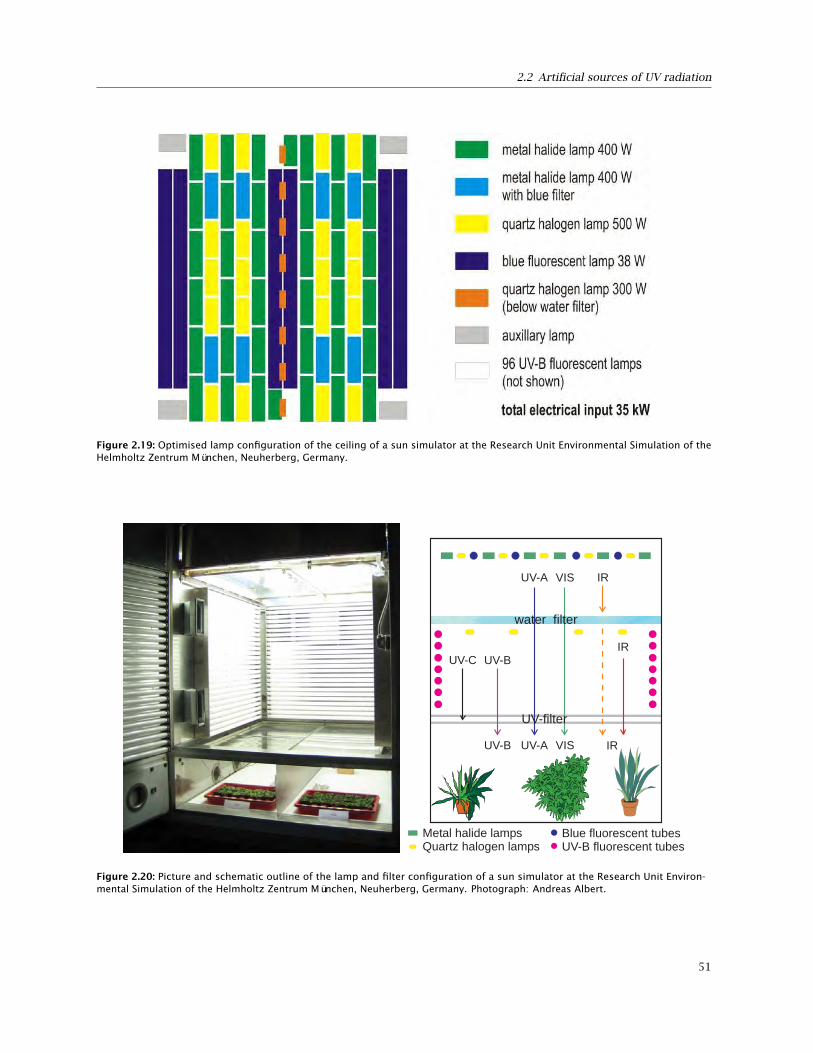
2.2 Artificial sources of UV radiation

Figure 2.19: Optimised lamp configuration of the ceiling of a sun simulator at the Research Unit Environmental Simulation of theHelmholtz Zentrum München, Neuherberg, Germany.

UV-A

UV-A

VIS

VIS

IR

IR

IRUV-C UV-B

UV-B

UV-filter

Metal halide lampsQuartz halogen lamps

Blue fluorescent tubesUV-B fluorescent tubes

water filter

Figure 2.20: Picture and schematic outline of the lamp and filter configuration of a sun simulator at the Research Unit Environ-mental Simulation of the Helmholtz Zentrum München, Neuherberg, Germany. Photograph: Andreas Albert.

51

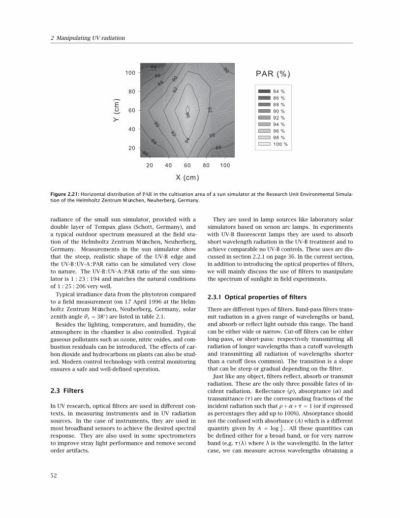
2 Manipulating UV radiation

Figure 2.21: Horizontal distribution of PAR in the cultivation area of a sun simulator at the Research Unit Environmental Simula-tion of the Helmholtz Zentrum München, Neuherberg, Germany.

radiance of the small sun simulator, provided with adouble layer of Tempax glass (Schott, Germany), anda typical outdoor spectrum measured at the field sta-tion of the Helmholtz Zentrum München, Neuherberg,Germany. Measurements in the sun simulator showthat the steep, realistic shape of the UV-B edge andthe UV-B :UV-A :PAR ratio can be simulated very closeto nature. The UV-B :UV-A :PAR ratio of the sun simu-lator is 1 : 23 : 194 and matches the natural conditionsof 1 : 25 : 206 very well.

Typical irradiance data from the phytotron comparedto a field measurement (on 17 April 1996 at the Helm-holtz Zentrum München, Neuherberg, Germany, solarzenith angle θs = 38) are listed in table 2.1.

Besides the lighting, temperature, and humidity, theatmosphere in the chamber is also controlled. Typicalgaseous pollutants such as ozone, nitric oxides, and com-bustion residuals can be introduced. The effects of car-bon dioxide and hydrocarbons on plants can also be stud-ied. Modern control technology with central monitoringensures a safe and well-defined operation.

2.3 Filters

In UV research, optical filters are used in different con-texts, in measuring instruments and in UV radiationsources. In the case of instruments, they are used inmost broadband sensors to achieve the desired spectralresponse. They are also used in some spectrometersto improve stray light performance and remove secondorder artifacts.

They are used in lamp sources like laboratory solarsimulators based on xenon arc lamps. In experimentswith UV-B fluorescent lamps they are used to absorbshort wavelength radiation in the UV-B treatment and toachieve comparable no UV-B controls. These uses are dis-cussed in section 2.2.1 on page 36. In the current section,in addition to introducing the optical properties of filters,we will mainly discuss the use of filters to manipulatethe spectrum of sunlight in field experiments.

2.3.1 Optical properties of filters

There are different types of filters. Band-pass filters trans-mit radiation in a given range of wavelengths or band,and absorb or reflect light outside this range. The bandcan be either wide or narrow. Cut-off filters can be eitherlong-pass, or short-pass: respectively transmitting allradiation of longer wavelengths than a cutoff wavelengthand transmitting all radiation of wavelengths shorterthan a cutoff (less common). The transition is a slopethat can be steep or gradual depending on the filter.

Just like any object, filters reflect, absorb or transmitradiation. These are the only three possible fates of in-cident radiation. Reflectance (ρ), absorptance (α) andtransmittance (τ) are the corresponding fractions of theincident radiation such that ρ+α+τ = 1 (or if expressedas percentages they add up to 100%). Absorptance shouldnot the confused with absorbance (A) which is a differentquantity given by A = log 1

τ . All these quantities canbe defined either for a broad band, or for very narrowband (e.g. τ(λ) where λ is the wavelength). In the lattercase, we can measure across wavelengths obtaining a

52

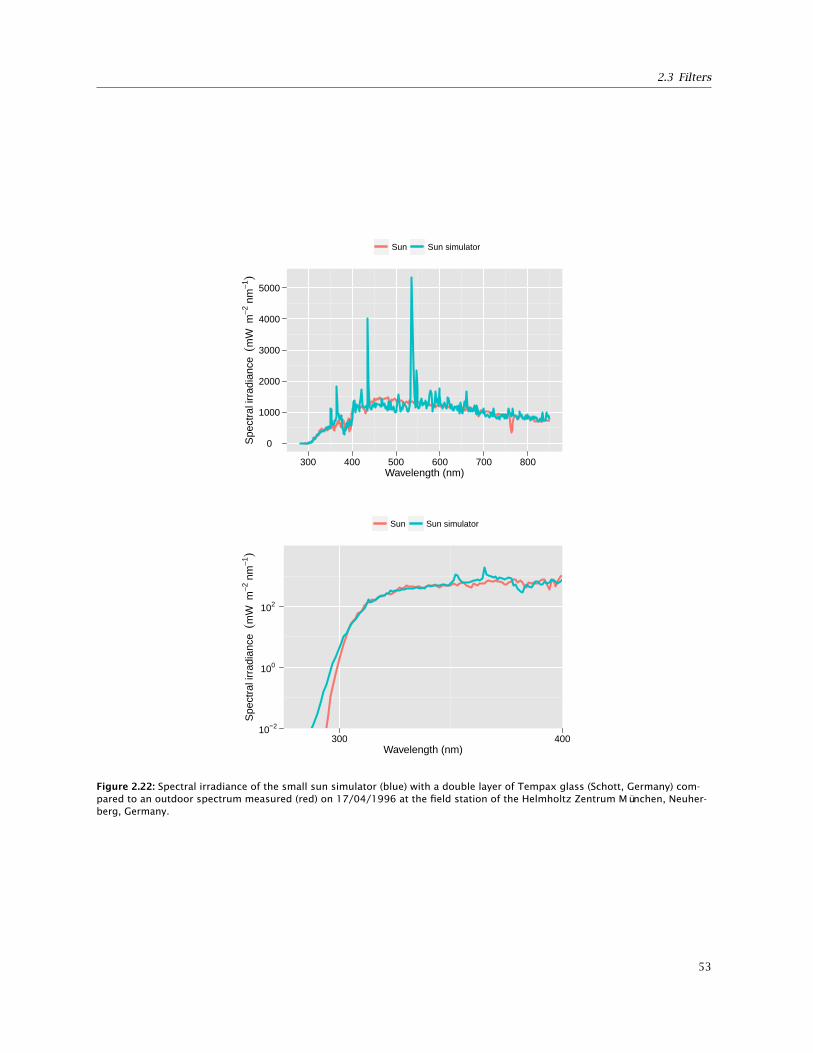
2.3 Filters

0

1000

2000

3000

4000

5000

300 400 500 600 700 800Wavelength (nm)

Spe

ctra

l irr

adia

nce

(mW

m−2

nm

−1)

Sun Sun simulator

10−2

100

102

300 400Wavelength (nm)

Spe

ctra

l irr

adia

nce

(mW

m−2

nm

−1)

Sun Sun simulator

Figure 2.22: Spectral irradiance of the small sun simulator (blue) with a double layer of Tempax glass (Schott, Germany) com-pared to an outdoor spectrum measured (red) on 17/04/1996 at the field station of the Helmholtz Zentrum München, Neuher-berg, Germany.

53

2 Manipulating UV radiation

Table 2.1: Typical irradiance data from the small sun simulator (Small) and the walk-in-size chambers (Large) compared to a typicaloutdoor measurement at the Helmholtz Zentrum München, Neuherberg, Germany. The irradiance values of the wavelength rangesare given in units of W m−2.

Small Large Outdoor

EUVB 1.53 1.20 1.10EUVA 54.9 22.7 47.2EPAR 430 250 390

spectrum.

When describing filters, the main property of interestis spectral transmittance. Most filters work by absorbingradiation of the unwanted wavelengths. However, somespecial filters work by reflecting the unwanted radiation.This is important when working with high power lightsources: reflecting filters warm up much less that ab-sorbing filters. An example of reflecting filters are the socalled heat mirrors, which reflect infra-red radiation.

For light absorbing filters, like many of those madefrom plastic or optical glass, the optical characteristicsdepend not only on the material but also on its thickness.For this reason it is important to always indicate bothtype and thickness when describing a filter. In manycases one can take advantage of this phenomenon whenplanning experiments as the cutoff wavelength dependson the thickness of the filter.

Another important property of filters is whether theyscatter radiation or not. When light is scattered the dif-fuse radiation component increases. For example, nor-mal glass does not scatter visible radiation while opaline(white glass) does. As the proportion of diffuse radiationin PAR affects canopy photosynthesis (Markvart et al.,2010; Okerblom et al., 1992; Urban et al., 2007, 2012) oneshould use filters with similar scattering properties forall treatments.

Filters can be made from optical glass, gelatine, andmany different synthetic organic compounds. In manycases, coloured substances are used as additives to thewhole thickness of the material but sometimes a layeris merely applied to the surface or between two layersof transparent material. Glass filters tend to be verystable, but many plastics and the additives they containreact when illuminated, and deteriorate gradually whenexposed to visible- and especially UV radiation. Filtersmade from optical glass are a more expensive than thosemade from plastics and tend to be readily available onlyin small sizes. Plastic films used as filters tend to beavailable in large sheets or rolls. Sometimes, liquid fil-ters, usually aqueous solutions of chemicals, can also beuseful (see Chapter 11 in Montalti et al., 2006, for spectraltransmittance for several liquid filters). Sampath-Wiley

and Jahnke (2011) describe a new type of liquid filterwhich makes it possible to obtain a realistic simulationof the solar UV spectrum under laboratory conditionsusing normal UV-B fluorescent lamps.

The engineering quality of atmospheric UV absorptionby glass filter techniques is sufficient for most plantexperiments. However, this method has its limitations.Strong UV exposure causes rapid ageing of borosilicateglass filters due to a physico-chemical effect known assolarisation. This originates in UV-induced changes inthe oxidation state of iron contaminants present in theglass matrix. The oxidation of Fe2+ to Fe3+ is accompan-ied by an absorption shift to longer wavelengths withinthe UV range. A decrease in the transmittance of freshglass filters occurs within their first few hours of use,followed by a more-gradual long-term decline. Hence,changes in transmission during an experiment can belargely avoided by the pre-ageing of new filters. In ad-dition, there is a gradient of ageing with the depth ofthe glass. Soda-lime glass exhibits very much reducedageing compared to borosilicate glass. The solarisationof the soda-lime glass ceases after a few hours of UVtreatment and this may be due to its lower content ofiron contaminants (Döhring et al., 1996).

2.3.2 Manipulating UV radiation in sunlight

When using plastic films in the field they need to be sup-ported in a way such that they remain in place even underwindy conditions and also so that rainwater does not ac-cumulate on top of them. It is important to be awarethat plastic filters modify the microclimate in severalways. If they absorb infra-red radiation, even if trans-parent at other wavelengths, they will alter the energybalance of plants and soil under them. This produces agreenhouse effect that increases temperatures. If they ab-sorb PAR they will affect photosynthesis, and even smalldifferences in PAR transmittance (τPAR) between treat-ments could be important. Plants are partially protectedfrom wind and completely shielded from rain by the fil-ters. In some cases even plasticizer additives (differentphthalates) added during plastic manufacture have been

54

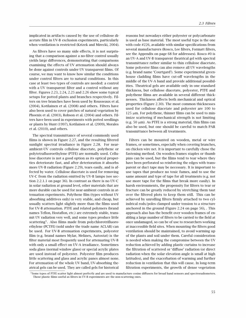
2.3 Filters

implicated in artifacts caused by the use of cellulose di-acetate film in UV-B exclusion experiments, particularlywhen ventilation is restricted (Krizek and Mirecki, 2004).

As filters have so many side effects, it is not surpris-ing that a comparison against a no-filter control usuallyyields large differences, demonstrating that comparisonsexamining the effects of UV attenuation should alwaysbe done against controls under UV transparent films. Ofcourse, we may want to know how similar the conditionsunder control filters are to natural conditions. In thiscase at least two types of controls are needed: a controlwith a UV transparent filter and a control without anyfilter. Figures 2.23, 2.24, 2.25 and 2.26 show some typicalsetups for potted plants and branches respectively. Fil-ters on tree branches have been used by Rousseaux et al.(2004), Kotilainen et al. (2008) and others. Filters havealso been used to cover patches of natural vegetation byPhoenix et al. (2003), Robson et al. (2004) and others. Fil-ters have been used in experiments with potted seedlingsor plants by Hunt (1997), Kotilainen et al. (2009), Moraleset al. (2010), and others.

The spectral transmittance of several commonly usedfilms is shown in Figure 2.27, and the resulting filteredsunlight spectral irradiance in Figure 2.28. For near-ambient-UV controls cellulose diacetate, polythene orpolytetrafluoroethylene (PTFE) are normally used. Cellu-lose diacetate is not a good option as its optical proper-ties deteriorate fast, and after deterioration it absorbsmore UV-B radiation (Figure 2.29), tears easily, and is af-fected by water. Cellulose diacetate is used for removingUV-C from the radiation emitted by UV-B lamps (see sec-tion 2.2.1.1 on page 36). In contrast as there is no UV-Cin solar radiation at ground level, other materials that aremore durable can be used for near-ambient controls in at-tenuation experiments. Polythene film (types without UVabsorbing additives only) is very stable, and cheap, butusually scatters light slightly more than the films usedfor UV-B attenuation. PTFE and related polymers (brandnames Teflon, Hostaflon, etc.) are extremely stable, trans-mit UV radiation very well, and some types produce littlescattering5. Also films made from polychlorotrifluoro-ethylene (PCTFE) (sold under the trade name ACLAR) canbe used. For UV-B attenuation experiments, polyesterfilm (e.g. brand names Mylar, Melinex, Autostat) is thefilter material most frequently used for attenuating UV-Bwith only a small effect on UV-A irradiance. Sometimessoda glass (normal window glass) or special acrylic platesare used instead of polyester. Polyester film produceslittle scattering and glass and acrylic panes almost none.For attenuation of the whole UV band, UV-absorbing the-atrical gels can be used. They are called gels for historical

reasons but nowadays either polyester or polycarbonateis used as base material. The most useful type is the onewith code #226, available with similar specifications fromseveral manufacturers (Rosco, Lee filters, Formatt filters,see the Appendix on page 68 for addresses). Rosco #0 isan UV-A and UV-B transparent theatrical gel with spectraltransmittance rather similar to thin cellulose diacetate.Some polyester films can also remove all UV wavelengths(e.g. brand name ‘Courtgard’). Some experimental green-house cladding films have cut-off wavelengths in themiddle of the UV-A band and provide additional possibil-ities. Theatrical gels are available only in one standardthickness, but cellulose diacetate, polyester, PTFE andpolythene films are available in several different thick-nesses. Thickness affects both mechanical and opticalproperties (Figure 2.30). The most common thicknessesused for cellulose diacetate and polyester are 100 to125 µm. For polythene, thinner films can be used to min-imize scattering if mechanical strength is not limiting(e.g. 50 µm). As PTFE is a strong material, thin films canalso be used, but one should be careful to match PARtransmittance between all treatments.

Filters can be mounted on wooden, metal or wireframes, or sometimes, especially when covering branches,on chicken wire net. It is important to carefully chose thefastening method. On wooden frames staples or thumbpins can be used, but the films tend to tear where theyhave been perforated so reinforcing the edges with trans-parent or duct tape may be necessary. It is important touse tapes that produce no toxic fumes, and to use thesame amount and type of tape for all treatments (e.g. notuse more tape for the films that break more easily). Inharsh environments, the propensity for filters to tear orfracture can be greatly reduced by stretching them tautover the filtered plots to keep them still. This can beachieved by unrolling filters firmly attached to two cyl-indrical rods/poles clamped under tension to a structureanchored in the ground (Figure 2.24 on page 56), . Thisapproach also has the benefit over wooden frames of en-abling a large number of filters to be carried to the field atonce undamaged, so can be of use to researchers workingat inaccessible field sites. When mounting the filters goodventilation should be maintained, to avoid warming upof the plants and soil under them. Careful considerationis needed when making the compromise between the UVreduction achieved by adding plastic curtains to increasethe filtration of scattered or ‘diffuse’ radiation (or directradiation when the solar elevation angle is small at highlatitudes), and the exacerbation of warming and furtherreduction in ventilation that this will cause. In long-termfiltration experiments, the growth of dense vegetation

5Some types of PTFE scatter light almost perfectly and are used to manufacture cosine diffusers for broad band sensors and spectroradiometers.Those plastic films useful as filters in UV-B experiments are the non-scattering ones.

55

2 Manipulating UV radiation

Figure 2.23: Filters in the field, mounted on wooden frames, and slightly tilted to avoid accumulation of rainwater. Viikki campus,University of Helsinki, Finland. Photograph: Pedro J. Aphalo.

Figure 2.24: Filters in the field, stretched between two metal rods. By rolling the film onto the rods, it can be kept under tension.The researchers are standing on wooden catwalks used for access to the plots. Ushuaia, Argentina. Photograph: Kevin Maloney.

56

2.3 Filters

Figure 2.25: Filter on a frame. The filter has narrow strips of one type of film on top of a base film of another material. Viikkicampus, University of Helsinki, Finland. Photograph: Pedro J. Aphalo.

Figure 2.26: Filters mounted on chicken wire net on tree branches. The underside of the branches is open to allow air circulationto prevent overheating. Note the strings that restrain the branch to prevent damage in windy weather. Kuohu, near Jyväskylä,Finland. Photograph: Titta Kotilainen.

57

2 Manipulating UV radiation

0

20

40

60

80

100

250 300 350 400 450 500Wavelength (nm)

Spe

ctra

l tra

nsm

ittan

ce (%

)

Rosco #226 Polyester 125 um Polythene 50 um MHCM09B

Figure 2.27: Transmittance spectra of several types of film used for altering the UV environment of plants. Rosco #226 is similarto Lee #226 and Formatt #226 films. MHCM09B is an experimental greenhouse film from BPI.Visqueen. The polyester film shownis Autostat CT5. The polythene is a generic product from Etola Oy (Finland) and 50 µm thick. Measurements were performed withan spectrophotometer equipped with an integrating sphere.

0.0

0.5

1.0

300 400 500 600 700 800Wavelength (nm)

Spe

ctra

l irr

adia

nce

(W m

−2 n

m−1

)

Ambient UV 0 UV A UV A+B

Figure 2.28: Spectral irradiance under of several types of film used for altering the UV environment of plants. UV 0: Rosco #226is similar to Lee #226 and Formatt #226 films. UV A: Polyester film (Autostat CT5, similar to Mylar). UV A+B: polythene (genericproduct from Etola Oy, Finland, 50 µm thick). Measurements were performed with a Maya 2000 Pro (Ocean Optics) with straylight, and slit function corrections. Measurements done during May 2012, in Helsinki, Finland under clear sky conditions, atnoon. The lines give the means from measurements under four replicate filters of each type, the grey band indicates ±1 s.e.Unpublished data of T. Matthew Robson and Saara Hartikainen.

58

2.3 Filters

0

20

40

60

80

100

280 300 320 340 360 380 400Wavelength (nm)

Spe

ctra

l tra

nsm

ittan

ce (%

)

0.0 h 3.0 h 5.4 h 9.0 h 15.0 h 27.0 h 45.0 h

0

20

40

60

80

100

280 300 320 340 360 380 400Wavelength (nm)

Spe

ctra

l tra

nsm

ittan

ce (%

)

Figure 2.29: Transmittance spectra of 115 µm thick cellulose diacetate (top) and 125 µm thick polyester (bottom) films exposedto radiation from Q-Panel UVB-313 lamps at 25 cm distance in a greenhouse. Total time in the greenhouse was the same (9 d),but daily irradiation varied among the different samples. Measurements done with an array detector spectrophotometer notequipped with an integrating sphere. Data measured by Tania de la Rosa.

under and around the filters is a common problem whichcan lead to large unwanted changes in the microclimatein experimental plots.

The impracticality of filtering entire trees means thatbranch filters are often the most acceptable substituteswhen assessing the effects of solar UV radiation on trees.However their installation and maintenance involves sev-eral additional considerations beyond those attached tofixed frames. Branch filters should be located only on thetop and sides of branches, while the underside shouldbe left open for ventilation and access. A structure ofchicken wire and aluminium cables can maintain theshape of the filter while minimising contact between thefilter and the treated part of the branch, however theweight of the structure should be kept to a minimum toreduce shading and the risk of mechanical damage to thetree. Filters mounted on branches behave like flags in thewind, so branches on which filters are installed need tobe tethered to the ground or their movement stabilisedusing wooden canes attached to a different large branch

or limb of the tree, or preferably a combination of boththese restraints, so that they do not move un-naturally orbreak in windy weather. By necessity in such experiments,the filtered area is relatively small and requires frequentmaintenance to keep the shoots and leaves from growinginto the filter or growing too far away from the filterinto areas where they receive too much unfiltered anddiffuse UV radiation. Particular attention should be givento the orientation of branch filters on a tree. For instance,branches and filters orientated to the north receive a verydifferent dose of visible and UV radiation from those ori-entated to the south (Rousseaux et al., 2004). Comparingsimilar branches of the same tree under different filtra-tion treatments is an obvious way to reduce the randomvariability among experimental units, but it is importantto be aware that signals could potentially pass betweendifferent filtered branches and unfiltered branches whichmay dilute the response of a particular branch to its UVtreatment. One method of controlling for communica-tion between branches involves excising the phloem of

59

2 Manipulating UV radiation

020406080

100

200 400 600 800 1000Wavelength (nm)S

pect

ral t

rans

mitt

ance

(%) Acetate film, 115 um Acetate film, 250 um Acetate film, 480 um

0

20

40

60

80

100

280 300 320 340 360 380 400Wavelength (nm)

Spe

ctra

l tra

nsm

ittan

ce (%

)

Figure 2.30: Transmittance spectra of new cellulose diacetate films of different thickness. Measurements made with an arraydetector spectrophotometer not equipped with an integrating sphere.

filtered branches. However, this isolation brings otherproblems as the realism of the experiment is reduced, sothe need to adopt this approach will depend on the aimsof each individual experiment. Maintaining branch filtersin situ during the autumn and winter is not always prac-tically feasible, however when using species that havedeterminate growth, their environment, particularly theradiation they receive, during bud set and the formationof leaf primordia can influence subsequent growth andleaf traits during the following growing season.

Sometimes the design of an experiment requires in-termediate levels of UV attenuation, and this can beachieved by mounting strips of one type of plastic film ona base of another type (Figure 2.25). In such a system thestrips are usually fastened at the edges of the wooden orwire frame on which the whole filter is attached. Unlessthe frames are small (less than 30 to 50 cm long sides) itmay also be necessary to attach the strips in the middlewith tape. In such a case the tape used must be clear toboth PAR and UV radiation. The cheapest old-fashionedstationery tapes use a cellulose acetate substrate and aregood for this purpose (e.g. Scotch Crystal Clear). Stripsare usually 10 to 15 mm wide and if the desired effectis 50% attenuation, they are attached with a separationequal to their own width. Cutting the strips with scissorsis a big task, but printers’ shops can usually cut them effi-

ciently for a small charge. The UV irradiance under filterswith strips is heterogeneous but the patches move withsolar transit through the sky. This is more of a problemfor measurement of irradiances than for the applicationof the treatments as reciprocity between irradiation timeand irradiance apparently holds for such experiments(de la Rosa et al., 2001).

Even if we use filters that are totally opaque to UV-B,the treatment will not lead to total UV-B exclusion. Thatis why we use the phrase ‘UV-B attenuation’ for suchtreatments (Figure 2.31). As discussed in section 1.4 onpage 8, solar UV radiation includes a large proportionof diffuse radiation coming from the sky, even undernon-cloudy conditions. Consequently, some UV radiationpenetrates under the edges of filters. It is therefore ne-cessary to avoid locating experimental plants near theedges of the filters, and we recommend to have at leastone row of border plants, forming a so-called ‘guard row’,from which no data are collected. Furthermore, it is pos-sible to use curtains of the same filter material on thesides of the frames, but one should not close all sides asair movement is needed to avoid elevated temperaturesand unnaturally still air. The filters should not be toohigh above the plants and irradiance should be measuredat all the different positions where measured plants arelocated, rather than just under the centre of the frame.

60

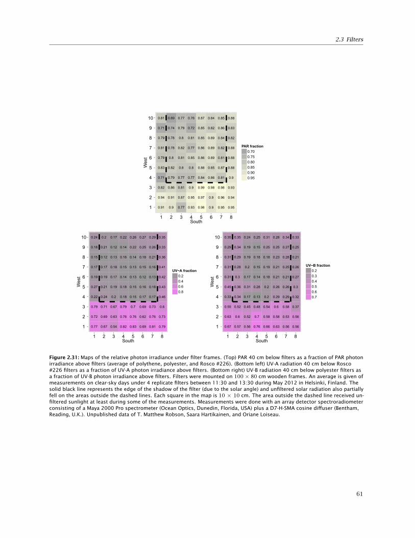
2.3 Filters

1

2

3

4

5

6

7

8

9

10 0.81

0.71

0.79

0.81

0.79

0.83

0.71

0.82

0.94

0.91

0.69

0.74

0.78

0.78

0.8

0.82

0.79

0.86

0.91

0.9

0.77

0.79

0.8

0.82

0.81

0.8

0.77

0.81

0.87

0.77

0.76

0.72

0.81

0.77

0.85

0.8

0.77

0.9

0.95

0.93

0.87

0.85

0.85

0.86

0.86

0.88

0.84

0.99

0.97

0.98

0.84

0.82

0.89

0.89

0.89

0.85

0.86

0.98

0.9

0.9

0.85

0.86

0.84

0.82

0.81

0.87

0.81

0.98

0.96

0.95

0.88

0.83

0.82

0.88

0.88

0.88

0.9

0.93

0.94

0.95

1 2 3 4 5 6 7 8South

Wes

tPAR fraction

0.700.750.800.850.900.95

1

2

3

4

5

6

7

8

9

10 0.24

0.18

0.15

0.17

0.19

0.27

0.22

0.79

0.72

0.77

0.2

0.21

0.12

0.17

0.19

0.21

0.24

0.71

0.69

0.67

0.17

0.12

0.13

0.18

0.17

0.19

0.2

0.67

0.63

0.54

0.22

0.14

0.16

0.15

0.14

0.18

0.18

0.79

0.76

0.82

0.26

0.22

0.14

0.13

0.13

0.15

0.15

0.7

0.76

0.83

0.27

0.25

0.18

0.15

0.12

0.16

0.17

0.69

0.62

0.69

0.29

0.26

0.21

0.16

0.13

0.18

0.17

0.73

0.76

0.81

0.35

0.33

0.36

0.41

0.42

0.43

0.46

0.6

0.73

0.79

1 2 3 4 5 6 7 8South

Wes

t

UV−A fraction0.20.40.60.8

1

2

3

4

5

6

7

8

9

10 0.35

0.29

0.31

0.31

0.31

0.45

0.33

0.55

0.63

0.67

0.35

0.34

0.29

0.28

0.3

0.36

0.34

0.52

0.6

0.57

0.24

0.19

0.19

0.2

0.17

0.31

0.17

0.45

0.52

0.56

0.25

0.15

0.18

0.15

0.14

0.28

0.13

0.48

0.7

0.76

0.31

0.25

0.18

0.19

0.18

0.2

0.2

0.54

0.58

0.66

0.28

0.25

0.23

0.21

0.21

0.26

0.29

0.6

0.58

0.63

0.34

0.27

0.28

0.25

0.21

0.26

0.29

0.58

0.53

0.56

0.33

0.25

0.21

0.26

0.27

0.3

0.32

0.37

0.56

0.56

1 2 3 4 5 6 7 8South

Wes

t

UV−B fraction0.20.30.40.50.60.7

Figure 2.31: Maps of the relative photon irradiance under filter frames. (Top) PAR 40 cm below filters as a fraction of PAR photonirradiance above filters (average of polythene, polyester, and Rosco #226). (Bottom left) UV-A radiation 40 cm below Rosco#226 filters as a fraction of UV-A photon irradiance above filters. (Bottom right) UV-B radiation 40 cm below polyester filters asa fraction of UV-B photon irradiance above filters. Filters were mounted on 100 × 80 cm wooden frames. An average is given ofmeasurements on clear-sky days under 4 replicate filters between 11:30 and 13:30 during May 2012 in Helsinki, Finland. Thesolid black line represents the edge of the shadow of the filter (due to the solar angle) and unfiltered solar radiation also partiallyfell on the areas outside the dashed lines. Each square in the map is 10 × 10 cm. The area outside the dashed line received un-filtered sunlight at least during some of the measurements. Measurements were done with an array detector spectroradiometerconsisting of a Maya 2000 Pro spectrometer (Ocean Optics, Dunedin, Florida, USA) plus a D7-H-SMA cosine diffuser (Bentham,Reading, U.K.). Unpublished data of T. Matthew Robson, Saara Hartikainen, and Oriane Loiseau.

61

2 Manipulating UV radiation

2.3.3 Measuring the spectral transmittance offilters

The recommended instrument for measuring filter spec-tral transmittance is a spectrometer or spectrophoto-meter equipped with an integrating sphere. Using anintegrating sphere ensures that all transmitted radiation,both non-scattered and scattered is taken into accountin the measurement. For non-scattering filters, one canobtain a reasonable approximation of the total spectraltransmittance with a regular spectrophotometer. In mostcases it is adequate to cut a piece of the film to the sizeof a cuvette and insert it carefully in the cuvette holder.In some models with an open light path (e.g. HP 8453,Hewlett Packard Gmbh, Waldbronn, Germany, now Agi-lent) it is possible to put a larger piece of filter materialin the light path outside the cuvette holder but close to it.For measuring in the UV-B band one needs an instrumentusing a deuterium lamp as radiation source. The spectralresolution is important, and ideally should be 1 or 2 nm.

The optical properties of all filters change with time,even if the material from which they are made is stable,because filters get scratched and dirty. Dust and pollenstick to the filter surfaces and particles attach more tena-ciously to some materials than others so that the filtersin some treatments may become dirtier than in others.In addition to cleaning and replacing the filters regularly,it is necessary to measure the spectral transmittanceof both new and used filters. We also recommend thatsamples of the filters are taken both at the start and endof their use and are stored protected from light and heatat least until the results of the experiments have beenpublished, but preferably for longer.

2.4 Manipulating UV-B in the aquaticenvironment

2.4.1 Incubations in the field

In contrast to the situation in terrestrial environments,field experimentation with aquatic organisms is con-strained not only by the underwater light conditions butalso by a suite of physical perturbations (e.g. wave action,tidal fluctuations, currents, sedimentation, etc.). In thecase of benthic macrophytes, an important factor thathas to be considered is their vertical distribution. Deepor constantly submerged environments impose differentdifficulties compared to e.g. intertidal locations, whichare subjected to changing light conditions due to theaction of tides. In lakes and rivers, differences in theconcentration of suspended UV absorbing substancesbetween the surface and deeper habitats can be import-ant. An experimental design for the study of seaweeds

normally includes different filters cutting-off UV-B andUV-A (see section 2.3 for details).

Algae can be exposed to these different radiation con-ditions by using self-made incubators constructed withplastic frames and nets with different diameters andforms depending of the size of the macrophyte (Figure2.32). Both the cylindrical and sheet Plexiglass incubat-ors can be covered by appropriate UV cut-off films andlocated at different water depths by using ropes or buoys.E.g. as used by Gómez et al. (2005) with the red alga Gra-cilaria chilensis in the Quempillen Estuary (Chile). Thecylindrical incubators can be also used in intertidal pools,allowing them to float or locating them at the bottom ofa pool. In general, experiments dealing with effects ofnatural UV radiation on aquatic organisms are carriedout in a range of depths between 0 and 10 m to representthe UV penetration depth in coastal waters.

The diurnal variability of solar radiation is one of themost important factors to consider when working withaquatic macrophytes in the field. In general, at tem-perate and cold-temperate locations, daily changes inthe irradiance conditions are also exacerbated by depth,which affects the number of hours during which algae areexposed to UV radiation. It is well known that photosyn-thetic physiology changes during the day with maximumrates of photoinhibition (a mechanism of dissipation ofexcess energy) occurring during the highest solar irradi-ance at midday, while a recovery in the photosyntheticcapacity is found in the afternoon (Figueroa et al., 1997;Gómez et al., 2004; Häder et al., 1996). This pattern iswell generalized in macrophytes and strongly depend-ent on the growth depth: individuals growing at shallowdepths show a more efficient photoinhibition than theirdeeper counterparts (Franklin and Forster, 1997). Thus,experimental designs employing transplantation or in-cubations at different depths along the water columnshould consider these potential confounding effects.

Tides are also a relevant factor affecting UV radiationin shallow marine waters, especially for intertidal species.Fluctuations in the height of the water column causedby tidal regimes can reduce or increase considerably theavailable UV radiation. For example, in a study comparingtwo coastal systems with different tidal range, Huovinenand Gómez (2011) demonstrated that algae from fjords,with tidal ranges close to 7 m, exhibited less differencein photosynthetic light demand and susceptibility to UVradiation than algae from an open coast where maximaltidal variation was 2 m. Probably, this is a major factorinfluencing experimentation with benthic intertidal mac-rophytes, especially in highly dynamic systems that mayalso be characterized by strong wave action.

62

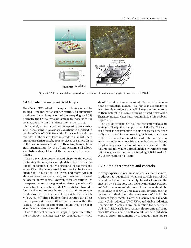
2.5 Suitable treatments and controls

Figure 2.32: Experimental setup used for incubation of marine macrophytes to underwater UV fields.

2.4.2 Incubation under artificial lamps

The effect of UV radiation on aquatic plants can also bestudied using incubations under controlled illuminationconditions (using lamps) in the laboratory (Figure 2.33).Normally the UV sources are similar to those used forincubations of terrestrial plants (see section 2.2.1).

In general, experimentation on aquatic plants usingsmall vessels under laboratory conditions is designed totest for effects of UV in isolated cells or small sized mac-rophytes. In the case of large seaweeds (e.g. kelps), spacelimitation restricts incubations to pieces or sample discs.In the case of seaweeds, due to their simple morpholo-gical organization, the use of cut sections still allowsa realistic extrapolation of the situation in the wholethallus.

The optical characteristics and shape of the vesselscontaining the samples strongly determine the orienta-tion of the sample to the UV source and the experimentalsetup. Often the vessels used in routine incubations areopaque to UV radiation (e.g. Pyrex, and many types ofglass ware and polycarbonate), and thus lamps shouldbe located above them. However, there are various UVtransparent materials, e.g. methacrylate (Type GS-2458)or quartz glass, which permits UV irradiation from dif-ferent sides and mimics better the natural underwaterconditions. In experimental setups which cover vesselswith UV cut-off filters, bubbles from aeration can affectthe UV penetration and diffraction patterns within thevessels. Thus, cut-off and neutral filters should be keptat sufficient distance from the water.

Due to the heat emission of lamps, temperature withinthe incubation chamber can vary considerably, which

should be taken into account, similar as with incuba-tions of terrestrial plants. This factor is especially rel-evant for algae subject to small changes in temperaturein their habitat, e.g. some deep water and polar algae.Thermoregulated water baths can minimize this problem(Figure 2.33).

The use of artificial UV sources presents various ad-vantages. Firstly, the manipulation of the UV:PAR ratiocan permit the examination of some processes that nor-mally are masked by the prevailing high PAR irradiancesin the field, as well as simulations of different UV scen-arios. Secondly, it is possible to standardize conditionsfor physiology, a situation not normally possible in thenatural habitat, where unpredictable environment con-ditions (e.g. water motion, scattered light field) make insitu experimentation difficult.

2.5 Suitable treatments and controls

In every experiment one must include a suitable controlin addition to treatments. What is a suitable control willdepend on the aims of the study. In order to assess theeffect of UV-B radiation, then the only difference betweenan UV-B treatment and the control treatment should bethe irradiance of UV-B. This may seem obvious, but it isimportant to think about the consequence of this for thedesign of experiments. Many UV-B sources emit in addi-tion to UV-B radiation, UV-C, UV-A and visible radiation.Common UV-A sources emit in addition to UV-A, UV-C,UV-B and visible radiation. As most fluorescent and someother UV sources emit small amounts of UV-C radiation,which is absent in sunlight, UV-C radiation must be re-

63

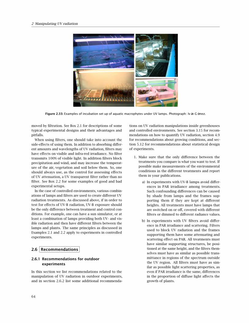
2 Manipulating UV radiation

Figure 2.33: Examples of incubation set up of aquatic macrophytes under UV lamps. Photograph: Iván Gómez.

moved by filtration. See Box 2.1 for descriptions of sometypical experimental designs and their advantages andpitfalls.

When using filters, one should take into account theside-effects of using them. In addition to absorbing differ-ent amounts and wavelengths of UV radiation, filters mayhave effects on visible and infra-red irradiance. No filtertransmits 100% of visible light. In addition filters blockprecipitation and wind, and may increase the temperat-ure of the air, vegetation and soil below them. So, oneshould always use, as the control for assessing effectsof UV attenuation, a UV transparent filter rather than nofilter. See Box 2.2 for some examples of good and badexperimental setups.

In the case of controlled environments, various combin-ations of lamps and filters are used to create different UVradiation treatments. As discussed above, if in order totest for effects of UV-B radiation, UV-B exposure shouldbe the only difference between treatment and control con-ditions. For example, one can have a sun simulator, or atleast a combination of lamps providing both UV- and vis-ible radiation and then have different filters between thelamps and plants. The same principles as discussed inExamples 2.1 and 2.2 apply to experiments in controlledexperiments.

2.6 Recommendations

2.6.1 Recommendations for outdoorexperiments

In this section we list recommendations related to themanipulation of UV radiation in outdoor experiments,and in section 2.6.2 list some additional recommenda-

tions on UV radiation manipulations inside greenhousesand controlled environments. See section 3.15 for recom-mendations on how to quantify UV radiation, section 4.9for recommendations about growing conditions, and sec-tion 5.12 for recommendations about statistical designof experiments.

1. Make sure that the only difference between thetreatments you compare is what you want to test. Ifpossible make measurements of the environmentalconditions in the different treatments and reportthem in your publications.

a) In experiments with UV-B lamps avoid differ-ences in PAR irradiance among treatments.Such confounding differences can be causedby shade from lamps and the frames sup-porting them if they are kept at differentheights. All treatments must have lamps thatare switched on or off, covered with differentfilters or dimmed to different radiance values.

b) In experiments with UV filters avoid differ-ence in PAR irradiance and scattering. Filtersused to block UV radiation and the framessupporting them have some attenuating andscattering effect on PAR. All treatments musthave similar supporting structures, be posi-tioned at the same height, and the filters them-selves must have as similar as possible trans-mittance in regions of the spectrum outsidethe UV region. All filters must have as sim-ilar as possible light scattering properties, aseven if PAR irradiance is the same, differencesin the proportion of diffuse light affects thegrowth of plants.

64

2.6 Recommendations

Box 2.1: Treatments and controls when using lamps in the field

Case We use Q-Panel UVB-313 tubes, or Philips TL12 fluorescent tubes outdoors. These lamps are sold asbroadband UV-B lamps, but they emit radiation of other wavelengths (UV-C, UV-A, and visible) in additionto UV-B (see Figure 2.2 on page 37). Our objective is to study the effect of UV-B radiation.

Design 1 We remove UV-C from the UV-B treatment by filtering the lamps with cellulose diacetate (see Figure2.27 on page 58). We add UV-A (and a very small amount of visible radiation) to the controls by havingidentical lamps as in the treatments but filtered with polyester film, which absorbs UV-C and UV-B. Thisalso ensures that any effect of the lamps on the temperature of plants is similar in treated and controlplants, and shading of sunlight is similar. This type of control is usually called ‘UV-A control’.

Design 2 As above, but in addition we add a second control with unenergized lamps. We can compare thiscontrol to the UV-A control to assess whether there is any side effect related to the functioning of the lampsbut unrelated to UV-B radiation.

Design 3 We add a third control with no lamps or frames. By comparing this control with the control withunenergized lamps we can test for the effect of shading by lamps and supporting structures.

Design 4 We use cellulose diacetate-filtered UV-B lamps for treatments and unenergized lamps for controls. Inthis case the effect of UV-B is confounded with other effects of the UV-B lamps, except for shading.

Design 5 We use cellulose diacetate-filtered UV-B lamps for treatments and no lamps or frames for the controls.In this case the effect of UV-B is confounded with all other effects of using lamps.

Caveat When discussing very small effects of treatments and the different controls there is always the riskof misinterpretation as the films used as filters are far from perfect, there is a transition zone betweenhigh absorptance and high transmittance spanning tenths of nanometres in wavelength (see Figure 2.27).Consequently, UV-A controls will not be exposed to exactly the same irradiance of UV-A as UV-B treatedplants. Usually they will be exposed to a slightly lower irradiance of UV-A plus a trace of UV-B.

Comparison Design 1 is the simplest design that can be used to test for the effects of UV-B. Design 2, is preferableas it allows an assessment of the possible secondary effects of lamps, except for shading. Design 3, is rarelyused, but allows an assessment all side-effects of lamps in addition to the effect of UV-B. Is useful in anecological context where we are interested in assessing how much the experimental setup disrupts naturalconditions. Design 4 should be avoided as it is unsuitable for testing the effects of UV-B radiation as allthe different effects of the lamps are confounded with the effect of UV-B enhancement, except for shade.Design 5 is the worst possible, and should never be used.

c) In experiments with UV-B lamps avoid differ-ences in temperature among treatments. Keepthe distance between UV lamps and the top ofthe plants at least 0.4–0.5 m. If enclosures likeopen-top chambers are used, provide enoughventilation or cooling to remove the heat gen-erated by the lamps.

d) In experiments with UV filters avoid differ-ences in temperature among treatments. Themain factor to consider in this case is ventila-tion and distance from the film to the top ofthe plants. An additional factor is the trans-mittance of the different films to longwave

infra-red radiation. The filters can affect thetemperatures both during the day and at night.If possible, measure the temperature of theplants and soil, in addition to the temperatureof the air.

e) In experiments with UV filters avoid artifactscaused by plasticisers used in some plasticfilms used as filters. Ensure good ventilationand if possible avoid using cellulose diacetatefilms for near-ambient controls. When not us-ing lamps there is no need to remove UV-Cradiation and consequently the more stableand less toxic PTFE (Teflon) or polythene films

65

2 Manipulating UV radiation

Box 2.2: Treatments and controls when using filters in the field

Case We use polyester (‘Mylar’) film outdoors to attenuate UV-B radiation (see Figure 2.28 on page 58). Ourobjective is to study the effect of solar UV-B radiation.

Design 1 We attenuate UV-B radiation (but not UV-A radiation) in the −UV-B treatment by filtering sunlight witha polyester film. We use as a control a film that transmits UV-B and UV-A. This ensures that most of theeffect of the films on precipitation, wind and temperature is similar for treated and control plants. Alsoshading of sunlight by supporting structures is similar. This type of control is usually called ‘near ambientUV control’.

Design 2 As above, but in addition we add a second treatment with a filter absorbing both UV-A- and UV-Bradiation. We can compare this treatment to the UV-B attenuation treatment to assess whether there is aneffect of UV-A radiation.

Design 3 We add a second control without filters or frames (‘ambient control’). By comparing this control withthe near-ambient control we can test for the effect of filters and supporting structures.

Design 4 We attenuate UV-B radiation in our −UV-B treatment by filtering sunlight with a polyester film. Wehave as controls plots with no filters or supporting structures. In this case the effect of UV-B is confoundedwith other effects of the filters.

Caveat When discussing very small effects of treatments and the different controls there is always the risk ofmisinterpretation as the films used as filters are far from perfect, there is a transition zone between highabsorptance and high transmittance spanning tenths of nanometres in wavelength (see Figure 2.27 on page58). Consequently, near ambient UV controls will not be exposed to exactly the same irradiance of UV-A asplants under the UV-B-attenuation treated plants. Usually they will be exposed to a slightly lower irradianceof UV-A plus a trace of long wavelength UV-B.

Comparison Design 1 is the simplest design that can be used to test for the effects of UV-B. Design 2, ispreferable as it allows us to also assess the effects of solar UV-A radiation. Design 3, is not always used, butallows to assess all side-effects of filters in addition to the effect of UV radiation. This design is useful in anecological context where we are interested in assessing how much our experimental setup disrupts naturalconditions. Design 4 should be avoided as it is unsuitable for testing the effects of UV-B radiation as all thedifferent effects of the filters are confounded with the effect of UV-B attenuation.

should be used instead.

2. In experiments with UV-B lamps do not use un-filtered lamps. Most UV-B lamps also emit someUV-C that must be filtered with a cellulose diacet-ate filter in UV-B treated plots. Most UV-B lampsalso emit UV-A, so an additional UV-A controlshould be included in all experiments. This controlis achieved by filtering out both UV-C and UV-Bradiation by means of polyester film. The smal-lest well designed experiment should include threetreatments: (i) a control with unenergized lamps,(ii) an UV-A control with polyester filtered lamps,and (iii) an UV-B treatment with cellulose diacetatefiltered lamps.

3. If the difference between near-ambient controls andtrue ambient conditions is of interest, then an addi-tional true ambient control should be included totest how big is the effect of the small differences inair, soil and leaf temperatures, PAR irradiance, airhumidity and any other side-effect of the manipu-lations. In any case, when designing an experimentwe should strive to minimize shading, alterationsin temperature and ventilation.

4. In experiments with UV-B lamps, if at all possible,use modulated systems that avoid unrealistic ratiosbetween UV- and PAR irradiances. If the use of amodulated system is impossible, keep the lamps ononly a few hours centred on solar noon and switchthem off during cloudy weather.

66

2.7 Further reading

5. In experiments with UV-B lamps use high frequencyelectronic ballasts rather than electromagnetic bal-lasts to drive the lamps, so as to avoid flicker inthe UV radiation output, which can affect insectbehaviour.

6. In all experiments using filters check periodicallywhether the spectral characteristics of the filtershave changed and replace them when needed. Cel-lulose diacetate degrades particularly fast and, forexample when used at about 0.3 m from UV-Blamps it should be replace after about 50 h of lampirradiation. If wrapped on lamps, it should be re-placed even more frequently. These times are ap-proximate and can also be extended when usingmodulated systems.

7. In experiments using filters to attenuate UV in sun-light, even if the filters are not yet degraded orif they are made of stable materials like glass orPFTE (Teflon) the transmission characteristics willchange by the accumulation of dust, dirt and pol-len. If this happens, the filters should be cleanedor replaced.

2.6.2 Recommendations for experiments ingreenhouses and controlled environments

Many of the recommendations in section 2.6.1 can beadapted to apply to indoor experiments. Here we listadditional recommendations applicable to experimentsin greenhouses and controlled experiments.

1. Keep the balance between UV-B irradiance, UV-Airradiance and PAR as similar as possible to that insunlight and/or vegetation canopies. Many growthchambers and growth rooms achieve relatively lowirradiances of PAR. Avoid using high doses of UV-Bin such cabinets. Some chambers and rooms havesheets of polycarbonate (PC) separating the lampsfrom the plants, in such chambers UV levels arenegligible. In chambers using bare lamps, UV-A ir-radiance is unrealistically low, but usually not equalto zero. A visible- and UV radiation spectral com-position truly matching sunlight can be achievedonly with sun simulators.

2. Unless you are specifically studying the effect ofstep changes in UV-B irradiance, for annual plantswe recommend that the UV-B treatment starts atthe time of seed germination or earlier, and forperennial plants before budburst.

3. In greenhouses, depending on the cladding mater-ial used, the UV-B and UV-A irradiances will differ

from those outdoors. Irradiances of PAR and UVare always somewhat lower than outdoors as thecladding materials and the structure of the green-house absorb part of the radiation.

4. Be aware that even though the temperature may beadequate for growing plants in a greenhouse duringthe winter, light and especially UV irradiances aremuch lower than in the summer, even when highpressure sodium or metal halide lamps are used toincrease PAR levels. For this reason, in experimentswith UV-B lamps the balance between PAR and UVcan become very different to that under naturalconditions.

5. Of course, if you are not interested in what hap-pens under natural conditions but are researchingthe management of crops under cover, then youonly have to make sure that your treatments matchwhat can be achieved in commercial productionsystems.

2.7 Further reading

The following links are to directives and recommenda-tions concerning protection from UV exposure.

http://eur-lex.europa.eu/LexUriServ/LexUriServ.do?uri=OJ:L:2006:114:0038:0059:EN:PDF (EU directive 2006/25/EC about protect-ing workers from optical radiation)http://www.hse.gov.uk/radiation/nonionising/optical.htm (guide on how toapply this directive (not approved yet by EU)http://www.who.int/uv/sun_protection/en/ (general recommendations by WHO)

2.8 Appendix: Calculating the radiation fieldunder an array of lamps

This section includes code for calculating the radiationfield under different arrays of lamps (Figures 2.5 and 2.6).The algorithm is that in the BASIC program in Björn andTeramura (1993) with a few changes related to the dens-ity of grid points used, and the area of the grid for whichthe light field is calculated. The grid area is expandedas it is also important to assess the distance at whichneighbouring arrays can be located. Please, see Björn andTeramura (1993) for the details of the algorithm. Thealgorithm assumes that there are no reflecting surfacesnear the array, so it is better suited for simulating thelight field under arrays of lamps located outdoors, thanfor those located in controlled environments.

67

2 Manipulating UV radiation

The functions are in the R package ‘lamps’ which isavailable from the handbook web site. The followingexample also uses package ggplot2, available from CRAN(comprehensive R archive network, at http://cran.r-project.org/ and many mirror sites). The firstexample (Box 2.3) is for calculating and plotting the ra-diation field under and array of fluorescent tubes, usingmostly the defaults. See the package documentation forthe many function arguments available. The second ex-ample shows how to draw the positions of the fluorescenttubes (Box 2.4).

2.9 Appendix: Suppliers of light sourcesand filters

In this section we provide names and web addresses tosome suppliers of light sources and filters. This is cer-tainly an incomplete list and exclusion reflects only ourignorance.UV lamps:http://www.lighting.philips.com/ (UV-Band many other types of lamps)http://www.q-lab.com/ (‘Q-Panel’ UV-A andUV-B lamps)Ballasts for fluorescent lampshttp://www.osram.com/ (‘Quicktronic’ electronicdimming ballasts)

http://www.tridonic.com/ (electronic dimmingballasts)LEDs:http://www.osram.com/http://www.lighting.philips.com/http://www.roithner-laser.com/http://www.valoya.com/Xenon arc lamps:http://www.newport.com/oriel/http://www.muller-elektronik-optik.de/Lasers:http://www.opotek.com (Tunnable UV lasers)http://www.roithner-laser.com/Filters:http://www.formatt.co.uk/ (theatrical ‘gels’)http://www.leefilters.com/ (theatrical ‘gels’)http://www.macdermidautotype.com/ (‘Auto-stat’ polyester film)http://www.nordbergstekniska.se (cellulosediacetate, Mylar and other films)http://www.rosco.com/ (theatrical ‘gels’)http://www.schott.com/ (glass filters, andspecial glasses)http://www.thermoplast.fi/ (‘Autostat’,‘Aclar ’, and many other types of films.

68

2.9 Appendix: Suppliers of light sources and filters

Box 2.3: Calculating and plotting the radiation field under an array of fluorescent tubes with R, using packages ‘lamps’ and‘ggplot2’.

library(lamps)library(ggplot2)# cosine arrangementlight_field45.data <- light_field() # default for z is 0.45light_field60.data <- light_field(z = 0.6)light_field30.data <- light_field(z = 0.3)# equidistantlight_field45_l.data <- light_field(cosine_dist = FALSE)light_field60_l.data <- light_field(z = 0.6, cosine_dist = FALSE)light_field30_l.data <- light_field(z = 0.3, cosine_dist = FALSE)# a simple figurefig1 <- ggplot(light_field45.data, aes(x = x, y = y, fill = c))fig1 <- fig1 + geom_tile() + geom_contour(aes(z = c), colour = "white",

binwidth = 0.1)fig1 <- fig1 + labs(x = "x (m)", y = "y (m)", fill = "relative\nirradiance")print(fig1)# facets, figure with six panels we prepare the data by row# bindinglen <- length(light_field45.data$x)irrad_all.data <- rbind(light_field30.data, light_field45.data,

light_field60.data, light_field30_l.data, light_field45_l.data,light_field60_l.data)

irrad_all.data$dist <- c(rep("'cosine' pattern", len * 3), rep("equidistant",len * 3))

irrad_all.data$distance <- rep(rep(c("z = 0.30 m", "z = 0.45 m","z = 0.60 m"), rep(len, 3)), 2)

# we draw the figurefig <- ggplot(irrad_all.data, aes(x = x, y = y, fill = c))fig <- fig + geom_tile() + geom_contour(aes(z = c), colour = "white",

binwidth = 0.1)fig <- fig + labs(x = "x (m)", y = "y (m)", fill = "relat.\nirrad.")fig <- fig + facet_grid(distance ~ dist) + coord_equal(ratio = 1)print(fig)

69

2 Manipulating UV radiation

Box 2.4: Calculating and plotting the lamp positions in an array of fluorescent tubes with R, using packages ‘lamps’ and‘ggplot2’.

library(lamps)library(ggplot2)# calculating the positions of the tubes in the arraypositions_cos.data <- tube_positions()positions_eq.data <- tube_positions(cosine_dist = FALSE)# row binding the datapositions.data <- rbind(positions_cos.data, positions_eq.data)# adding labelspositions.data$dist <- rep(c("'cosine' pattern", "equidistant"),

rep(length(positions_cos.data$x), 2))positions.data$fake_label <- factor(rep("lamps", length(positions.data$dist)))

# drawing the figurefig_x <- ggplot(data = positions.data, aes(x = x, y = y, colour = tube))fig_x <- fig_x + geom_line(size = 2) + coord_equal(ratio = 1)fig_x <- fig_x + facet_grid(fake_label ~ dist)fig_x <- fig_x + labs(x = "x (m)", y = "y (m)", colour = "tubes ")fig_x <- fig_x + ylim(c(-1.48/2, 1.48/2)) + xlim(c(-1.1, 1.1))print(fig_x)

70

3 Quantifying UV radiation

Lars Olof Björn, Andy McLeod, Pedro J. Aphalo, Andreas Albert, Anders V. Lindfors, Anu Heikkilä, Predrag Kolarž,Lasse Ylianttila, Gaetano Zipoli, Daniele Grifoni, Pirjo Huovinen, Iván Gómez, Félix López Figueroa

3.1 Basic concepts and terminology

3.1.1 Introduction to UV and visible radiation

In this section we will discuss the quantities, units andterminology used to describe visible and UV radiation,and explain how to use and interpret information aboutradiation. We will explain the basic concepts associatedwith quantifying radiation and how the different aspectsof this topic are applied to UV experimentation.

When describing experimental conditions we need toavoid all ambiguity, so that our results can be interpretedand experiments repeated. For this reason “Light intens-ity” and “amount of light”, which are ambiguous terms,should be avoided in scientific contexts unless it is madeabsolutely clear what they stand for.

Radiation always consists of different wavelength com-ponents, although we often use the term “monochro-matic” when the spectral range is narrow. Not even asingle photon can be assigned an exact wavelength. Asradiation also travels in various directions, it is also al-ways associated with a distribution of directions. Whenwe say “collimated radiation”, we mean that the angulardistribution is very narrow. When we say “scattered or‘diffuse’ radiation”, we mean that the angular distribu-tion is wide. In order to fully describe radiation, we musttherefore describe the distribution of its wavelength com-ponents (the spectral distribution) and their direction inaddition to “amount”. Polarization is another propertyof radiation, but it will not be dealt with here. Finally, weshould consider the time dimension; radiation changesover time. Radiation can be measured almost instantan-eously and expressed as a rate, or integrated over time.Consequently we must distinguish between total energy,or the total number (or total number of moles) of photons,and the energy-or-photons per unit time. The first casegives an accumulated quantity, and the second case givesa rate. A clear distinction should also be made between

the incident radiation on a target and the amount of ra-diation absorbed. When dealing with ionizing radiation,the term “dose” is always used to mean the radiation ab-sorbed, however the same term often designates incidentradiation when used in connection with ultraviolet-B andvisible radiation.

A comprehensive glossary of terms relating to vis-ible and ultraviolet radiation has been published byBraslavsky (2007). It can be downloaded from the Internet(see link in reference list).

3.1.2 Direction

Daylight radiation has two components: (a) radiation ar-riving directly from the sun, or direct radiation, and (b)radiation arriving from the sky, or scattered or ‘diffuse’radiation. Because it is very distant compared to its size,the sun behaves almost as a point source. For this reasondirect radiation at the Earth surface comes from a singledirection, so that its ‘rays’ are parallel or collimated. Dif-fuse radiation is due to scattering and reflection in theatmosphere, and arrives from the whole sky, its ‘rays’ arenot parallel. Diffuse radiation is not collimated.

Light meters and radiation sensors are usually calib-rated using radiation from (approximately) a single direc-tion, i.e., collimated radiation from a lamp, but in nature(where most plants live!) radiation is not collimated. Thesolar radiation reaching the ground on clear cloud-freedays as direct sunlight is rather well collimated, but in ad-dition to direct radiation there is diffuse radiation fromthe sky. Furthermore, radiation reflected by the groundand objects in the surroundings also contributes to thediffuse radiation received by plants. A plant scientistwishing to understand how plants use and react to radi-ation has to take both direct and diffuse radiation intoaccount.

Many radiation meters have a flat receiving surface,

71

3 Quantifying UV radiation

just like many plant leaves, and so should in principlebe well suited to measuring the radiation reaching a leaf.But if we are interested in the whole plant rather than asingle leaf the situation is different, since plants are three-dimensional not flat and different surfaces on the plantface in different directions. In such situations where wewish to obtain an approximate estimate of the quantity ofradiation incident on a plant, it is better to use a spherethan a flat radiation meter. This is achieved with a meas-uring instrument that is equally sensitive to radiationfrom any direction.

This brings us to the distinction between

1. Irradiance, i.e., radiation power incident on a flatsurface of unit area, and

2. Energy fluence rate (or fluence rate for short), i.e.,radiation power incident on a sphere of unit crosssection. The term fluence rate was introduced byRupert (1974).

Other terms with the same meaning as energy fluencerate are space irradiance, scalar irradiance and actinicflux. The latter is used mostly by atmospheric scientists.The term spherical irradiance has been used in similarcontexts, but means one quarter of the fluence rate. Vec-torial irradiance is just the same as irradiance.

Both irradiance and energy fluence rate, can also bedescribed in terms of photons. For item 1 above, thecorresponding photon nomenclature has not yet beenstandardised. It would be logical to use the term photonirradiance, but many people, especially in the photosyn-thesis field, use the term photon flux density and theabbreviation PFD (PPFD for photosynthetic photon fluxdensity). For item 2 the term photon fluence rate is wellaccepted among plant physiologists, but hardly amongscientists in general (for example meteorologists call it‘actinic flux’ or ‘scalar irradiance’). Energy fluence is theenergy fluence rate integrated over time. The word en-ergy is frequently omitted, so that ‘fluence’ has the samemeaning as ‘energy fluence’. In contrast, when ‘photonfluence’ is meant, the word ‘photon’ is always explicitlymentioned.

When giving a value for irradiance, the direction of theplane for which the irradiance is considered must be spe-cified. This is often the horizontal plane but will dependon the object studied: for instance, the surface a leaf isfrequently not horizontal. For collimated radiation (com-ing from a single direction), irradiance and fluence ratehave the same numerical value if the beam of radiation isperpendicular to the plane on which irradiance is meas-ured (Figure 3.1.A). For completely isotropic radiationcoming from above (equally from any direction abovethe horizontal) the fluence rate is twice the irradianceon a horizontal plane (Figure 3.1.C). Sometimes one may

also have to consider radiation from below, especially inaquatic environments (Figure 3.1.D).

When a delimited beam of radiation hits a plane sur-face perpendicularly, it results in the irradiance, E, butthe same beam when tilted at an angle α to the verticalwill be more spread out, and thus the irradiance will belower. More specifically, the irradiance will be E · cosα(Figure 3.1.B).

3.1.3 Spectral irradiance

When we deal with how a quantity of radiation varieswith wavelength, for instance when plotting a spectrum,we add “spectral” to the name of the quantity to give“spectral irradiance” and “spectral fluence rate”. We mustalso adjust the units to account for the width of the partof the spectrum that is included in the value specified (inphotobiology nm−1 is often used to indicate wavelengthinterval, but the scale can also be defined in terms ofwave number or frequency, as in, cm−1 or s−1 respect-ively).

3.1.4 Wavelength

It is impractical to always quantify radiation by giving itscomplete spectral composition; so simplifications haveto be made that account for the most important featuresof a spectrum. From a purely physical viewpoint, thereare two basic ways of quantifying radiation. Either weexpress the quantity related to the number of photons, orthe quantity related to the energy of radiation. When con-sidering radiation of a single wavelength, the energy of aphoton, or quantum (in a vacuum), is inversely propor-tional to the wavelength and the proportionality constantis Planck’s constant multiplied by the speed of light in avacuum (see section 1.3).

q(λ) = h · ν = h · cλ

(3.1)

where q(λ) is a quantum, or the amount of energy thatone photon has, h is Planck’s constant (h = 6.626×10−34

Js), ν is frequency, λ is wavelength, and c is the speedof light in a vacuum (c = 2.998× 108 m s−1). Please, seesection 1.4 on page 8 for a numerical example. Whendealing with a band of wavelengths it is necessary torepeat these calculations for each wavelength (in prac-tice a very narrow band) and only then integrate acrosswavelengths. For example, PAR in units of W m−2 is ob-tained by integrating the spectral irradiance from 400 to700 nm. As explained in Box 1.2 on page 7, to determinea quantity in terms of photons, an energetic quantity hasto be weighted by the number of photons, i.e. divided bythe energy of a single photon at each wavelength fromequation 3.1. To get moles of photons, the value has to bedivided further by Avogadro’s number (NA = 6.022×1023

72

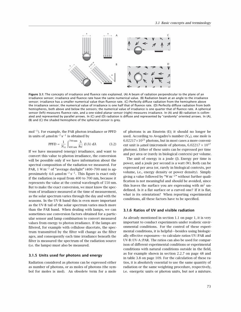
3.1 Basic concepts and terminology

α

a a co

s α

a aA

B

C

D

Figure 3.1: The concepts of irradiance and fluence rate explained. (A) A beam of radiation perpendicular to the plane of anirradiance sensor; irradiance and fluence rate have the same numerical value. (B) Radiation beam at an angle to the irradiancesensor; irradiance has a smaller numerical value than fluence rate. (C) Perfectly diffuse radiation from the hemisphere abovethe irradiance sensor; the numerical value of irradiance is one half that of fluence rate. (D) Perfectly diffuse radiation from bothhemispheres, both above and below the sensors; the numerical value of irradiance is one quarter that of fluence rate. A sphericalsensor (left) measures fluence rate, and a one-sided planar sensor (right) measures irradiance. In (A) and (B) radiation is collim-ated and represented by parallel arrows. In (C) and (D) radiation is diffuse and represented by “randomly” oriented arrows. In (A),(B) and (C) the shaded hemisphere of the spherical sensor is grey.

mol−1). For example, the PAR photon irradiance or PPFDin units of µmol m−2 s−1 is obtained by

PPFD = 1NA

∫ 700 nm

400 nm

λhcE(λ) dλ (3.2)

If we have measured (energy) irradiance, and want toconvert this value to photon irradiance, the conversionwill be possible only if we have information about thespectral composition of the radiation we measured. ForPAR, 1 W m−2 of “average daylight” (400–700 nm) is ap-proximately 4.6 µmol m−2 s−1. This figure is exact onlyif the radiation is equal from 400 to 700 nm, because itrepresents the value at the central wavelength of 550 nm.But to make the exact conversion, we must know the spec-trum of irradiance measured at the time of measurement,as the solar spectrum varies through the day and with theseasons. In the UV-B band this is even more importantas the UV-B tail of the solar spectrum varies much morethan the PAR band. When dealing with lamps, we cansometimes use conversion factors obtained for a partic-ular sensor and lamp combination to convert measuredvalues from energy to photon irradiance. If the lamps arefiltered, for example with cellulose diacetate, the spec-trum transmitted by the filter will change as the filterages, and consequently each time irradiance beneath thefilter is measured the spectrum of the radiation source(i.e. the lamps) must also be measured.

3.1.5 Units used for photons and energy

Radiation considered as photons can be expressed eitheras number of photons, or as moles of photons (the sym-bol for moles is mol). An obsolete term for a mole

of photons is an Einstein (E); it should no longer beused. According to Avogadro’s number (NA), one mole is6.02217×1023 photons, but in most cases a more conveni-ent unit is µmol (micromole of photons, 6.02217× 1017

photons). Either of these units can be expressed per timeand per area or (rarely in biological contexts) per volume.

The unit of energy is a joule (J). Energy per time ispower, and a joule per second is a watt (W). Both can beexpressed per area (or, rarely in biological contexts, pervolume, i.e., energy density or power density). Simplygiving a value followed by “W m−2” without further quali-fication is not meaningful and should be avoided, sincethis leaves the surface you are expressing with m2 un-defined. Is it a flat surface or a curved one? If it is flat,what is its orientation? When reporting experimentalconditions, all these factors have to be specified.

3.1.6 Ratios of UV and visible radiation

As already mentioned in section 1.1 on page 1, it is veryimportant to conduct experiments under realistic envir-onmental conditions. For the control of these experi-mental conditions, it is helpful—besides using biologic-ally effective exposures—to calculate ratios UV:PAR andUV-B :UV-A :PAR. The ratios can also be used for compar-ison of different experimental conditions or experimentalconditions with natural conditions outside in the field,as for example shown in section 2.2.7 on page 48 andin table 3.8 on page 109. For the calculation of these ra-tios, it is absolutely essential to use the same quantity ofradiation or the same weighting procedure, respectively,i.e. energetic units or photon units, but not a mixture.

73

3 Quantifying UV radiation

The term “energetic” means that the spectral irradianceis simply integrated over the respective spectral bandyielding units like W m−2. For the calculation of photonratios it is also necessary to integrate over the respectivespectral bands, but additionally weighted by the num-ber of photons at each wavelength (see section 3.1.4). Afunction to calculate photon ratios in R is described insection 3.19.4 on page 116.

3.1.7 A practical example

The importance of indicating the type of sensor and itsorientation is exemplified by the changing ratio of flu-ence rate to irradiance throughout a day (Figure 3.2). Atnoon, when the sun is high in the sky the ratio is at itsminimum. Even then the ratio remains larger than onebecause, other than at the equator, the midday sun neverreaches the zenith and because the sensor will also al-ways receive diffuse radiation from the whole sky. Wecan say that when measuring solar radiation the fluencerate will always be numerically larger than the irradi-ance. Towards both ends of the day the ratio reaches itsmaximum value because irradiance is being measuredon a horizontal plane but the sun is near the horizon.During twilight, particles in the atmosphere will makethe distribution of solar radiation more even, allowing arelatively large area of the sky to remain bright, and theratio decreases again.

3.1.8 Measuring fluence rate and radiance

Spherical sensors, as needed for measuring fluence rate,also called scalar irradiance, are not common. LI-COR(Lincoln, NE, USA) sells a spherical PAR quantum sensor(LI-193) that can be submerged, and Biospherical Instru-ments Inc. (San Diego, CA, USA) makes both PAR- (e.g.QSL-2100 and QSL-2200, terrestrial; QSP series with mod-els that can be submerged to thousands of metres) andalso narrowband spherical sensors for measuring UV-and visible radiation fluence rate. Biospherical Instru-ments Inc. also makes radiance sensors with input opticsthat have a very narrow acceptance angle. Figure 3.3shows the different entrance optics available for oneseries of sensors from Biospherical Instruments. Mostbroadband UV sensors and entrance optics for spectrora-diometers follow a cosine response. Björn (1995) de-scribes a method for estimating fluence rate from threeor six irradiance measurements at a series of specificangles.

3.1.9 Sensor output

Radiometer sensors can have either analog or digital out-puts. Some sensors with an analogue output have anamplifier next to the detector, others do not. Sensorswith an analog output are usually connected to a volt-meter or a datalogger. Some digital sensors are reallycomplete radiometers with a digital output. Examples ofradiometers with digital outputs, are shown in Figure 3.4.RS-232 and USB are digital interfaces frequently used toattach these sensors to personal computers1.

3.1.10 Calibration

To calibrate radiation sensors the relationship must bedetermined between the electrical signal produced by asensor and the amount of radiation impinging on thatsensor. The physical value of irradiance, E, of the incom-ing radiation in energy units, is obtained by “comparison”of a measurement X with that of a calibrated radiationsource Xlamp,

E = Elamp ·X · aXlamp

(3.3)

where Elamp is the calibration file of the lamp providedby the calibration survey. The factor a accounts for anydifference in the lamp to sensor distance between thesurvey’s calibration and your own measurement of thelamp. In most modern instruments this “comparison”is implicitly done by the software in the instrument it-self, or the computer it is attached to, by multiplyingthe electrical signal from the detector with a calibrationconstant. If this is not the case, it is necessary to correctall raw measurements, here X and Xlamp, before makingany further calculations, for example, by subtracting themeasurement of dark current (the sensor reading in thedark).

Although photons can be counted using a photomulti-plier and appropriate electronics, this approach does notprovide an absolute measurement. Some photons are al-ways missed and false counts are included due to thermalexcitation. Therefore, absolute calibration of radiationmeters can only be provided in energetic terms. For thispurpose so-called “blackbody radiators” of known tem-perature are used, since they depend only on temperaturefor the total radiation as well as its spectral distribution.Blackbody radiators used for the calibration of lamps,are then available for purchase by scientists for use assecondary standards.

In the case of broadband sensors used to measurebiologically-effective irradiances or selected bands of thespectrum, the calibration is usually carried out by com-parison to readings from a calibrated spectroradiometerunder a radiation source with a spectrum as similar as

1Many current computers, especially laptops, do not have an RS-232 interface but USB to RS-232 adaptors are readily available.

74

3.1 Basic concepts and terminology

1

2

3

4

5

6

08:00 10:00 12:00 14:00 16:00 18:00 20:00Time of day

Flue

nce

rate

: irr

adia

nce

measured model, no aerosol model, with aerosol

Figure 3.2: Ratio of fluence rate to irradiance throughout a summer day in southern Sweden under clear-sky conditions. Thegraph presents photosynthetically active radiation (PAR, 400–700 nm). For UV-B the diffuse component is proportionally largerthan for PAR due to scattering in the atmosphere (see section 1.4 on page 8 and Figure 1.6 on page 12) and consequently theratio at midday is also larger and the variation with time smaller. Under overcast sky conditions diffuse radiation predominatesand variation through the day is smaller than under clear sky conditions. Redrawn from Björn and Vogelmann (1996).

Figure 3.3: Different entrance optics used in USB radiometers of the ‘AMOUR’ series. From left to right: radiance, fluence rate(or scalar irradiance), irradiance and SMA connector. The SMA connector can be used to attach an optical fibre. Photograph © byBiospherical Instruments Inc.

75

3 Quantifying UV radiation

Figure 3.4: ‘AMOUR’ USB radiometers. Left: With a spherical diffuser for measuring fluence rate; right: with a planar cosinediffuser for measuring irradiance. Photograph © by Biospherical Instruments Inc.

possible to the one which will be measured with thebroadband sensor (e.g. sunlight). To calibrate spectrora-diometers, in addition to a spectral-irradiance calibrationagainst one or more lamps (with a continuous spectrum,such as an incandescent lamp), it is necessary to do awavelength calibration against the sun or a lamp (with aan emission spectrum with discrete, narrow and stablepeaks, such as a low pressure mercury lamp).

3.1.11 Further reading

Björn and Vogelmann (1996) treat the same subjects asthis section, but in more depth. Also the book edited byBjörn (2007) is a good source of basic information aboutradiation and photobiology.

3.2 Actinometry

Actinometers are chemical systems for the measurementof light and ultraviolet radiation. They do not need to becalibrated by the user, and thus do not require the pur-chase of an expensive standard lamp with an expensivepower supply. Standardization has usually been takencare of by those who have designed the actinometer. An-other advantage is that their geometry can more easilybe adjusted to the measurement problem. The shape ofa liquid actinometer can be made to correspond to theoverall shape of the irradiated object under study.

In many cases, it is of interest to study a suspensionor solution that can be put in an ordinary cuvette forspectrophotometry or fluorimetry, and the actinometersolution can be put into a similar cuvette. A large number

of actinometers have been devised. Kuhn et al. (1989)lists, briefly describes and gives references for 67 differ-ent systems of which they recommend five. In general,actinometers are sensitive to short-wave radiation (<500nm) and insensitive to long-wave radiation (>500 nm). In-sensitivity to long-wave radiation can be both a drawbackand an advantage, but by choosing the best actinometerfor a particular purpose we can avoid their disadvant-ages. One advantage of using an actinometer insensitiveto long wave radiation is that we can use it for UV workunder illumination visible to the human eye, without dis-turbing the measurement. Here we shall concentrate onthe most popular actinometer for ultraviolet radiation—the potassium ferrioxalate or potassium iron(III) oxalateactinometer. In addition to using it directly in some ex-periments, we can use it for checking the calibration ofother instruments, such as spectroradiometers.

The description below is sufficient for a researcherstarting to work in the field. For more detailed inform-ation one should consult Goldstein and Rabani (2008);Hatchard and Parker (1956); Lee and Seliger (1964); Parker(1953). Complete recipes have also been published, e.g.,Jagger (1967); Seliger and McElroy (1965). In the ferriox-alate actinometer the following photochemical reactionis exploited:

12 (COO)2−2 + Fe3+ + photon → CO2 + Fe2+

orOxalate ion + Fe(III) ion + radi-

ation → carbon dioxide + Fe(II) ion

The quantum yield for this reaction (i.e., the number

76

3.2 Actinometry

of iron ions reduced per photon absorbed) is slightlywavelength dependent but close to 1.26 in the spectralregion, 250–500 nm, where the ferrioxalate actinometeris used. Usually a 1-cm layer of 0.006 M ferrioxalate solu-tion is used. Quantum yield and the fraction of radiation(perpendicular to the 1 cm layer) absorbed are shown inTable 3.1.

As seen from Table 3.1 the sensitivity of this actino-meter (column to the right) is constant throughout mostof the UV range, which makes it very convenient for ourwork.

The amount of Fe(II) formed can be measured spec-trophotometrically after the addition of phenanthroline,which gives a strongly absorbing yellow complex withFe(II) ions.

The ferrioxalate (actually potassium ferrioxalate) forthe actinometer is prepared by mixing 3 volumes of 1.5M potassium oxalate (COOK2) with 1 volume of 1.5 MFeCl3 and stirring vigorously. This step and all the follow-ing procedures involving ferrioxalate should be carriedout under red light (red fluorescent tubes or LEDs). Theprecipitated K3Fe(C2O4)3·3H2O should be dissolved in aminimal amount of hot water and the solution allowedto cool for crystallization (this crystallization should berepeated twice more). Potassium ferrioxalate can also bepurchased ready-made, but the price difference encour-ages self-fabrication. The following is a recipe for thethree solutions required to carry out actinometry (seeGoldstein and Rabani, 2008, for a different procedureand other quantum yields):

Solution A: Dissolve 2.947 g of the purified and driedK3Fe(III) oxalate in 800 ml distilled water, add 100 ml0.5 M sulfuric acid, and dilute the solution to 1000 ml.This gives 0.006 M actinometer solution, which is suitablefor measurement of ultraviolet radiation.

Solution B: The phenanthroline solution to be used fordeveloping the colour with Fe(II) ions should be 0.1% w/v1:10 phenanthroline monohydrate in distilled water.

Solution C: Prepare an acetate buffer by mixing 600 mlof 0.5 M sodium acetate with 360 ml of 0.5 M H2SO4.

Solution A is irradiated with the radiation to be meas-ured. The geometries of both the container and of theradiation are important and must be taken into accountwhen evaluating the result. The simplest case is whenthe radiation is collimated, the container a flat spectro-photometer cuvette, the radiation strikes one face of thecuvette perpendicularly, and no radiation is transmitted.Even in this case one has to distinguish between whetherthe cuvette or the beam has the greater cross section, andcorrect for reflection in the cuvette surfaces. The irradi-ation time should be adjusted so that no more than 20%of the iron is reduced (this corresponds to an absorbanceof about 0.66). In the following we shall assume that we

use an ordinary fused-silica or quartz spectrophotometercuvette with 10 mm inner thickness and containing 3 mlactinometer solution.

After the irradiation and mixing of the actinometersolution, 2 ml of the irradiated solution is mixed with2 ml of solution B and 1 ml of solution C, and then di-luted to 20 ml with distilled water. After 30 minutesthe absorbance at 510 nm is measured against a blankmade up in the same way with unirradiated solution A.An absorbance of 0.5 corresponds to 0.905 µmol Fe2+.It is a good idea to check this relationship with knownamounts of FeSO4 if you have not previously checkedyour spectrophotometer for accuracy and linearity. Youshould not use any absorbance above 0.65.

Example of calculation: 3 ml of 0.006 M actinometersolution are irradiated by parallel rays of 300 nm UV-Bimpinging at right angles to one surface (and not ableto enter any other surface). The radiation cross sectionintercepted by the solution is 2 cm2. Five minutes ofirradiation produces an absorbance of 0.6. This cor-responds to 0.6 · 0.905/0.5 µmol = 1.086 µmol Fe2+,but since we have taken 2 out of the 3 ml actinometersolution for analysis, multiply by 3/2 to get the totalamount of Fe2+ formed. Throughout the UV-B regionthe quantum yield is 1.26, so this corresponds to ab-sorption of 3 · 1.086/2/1.26 µmol photons. Reflectionfrom the surface is estimated to be 7% (by applicationof Snell’s law, or law of refraction, giving the angle ofrefraction for an angle of incidence at the boundary oftwo media like water and glass). None of the radiationpenetrates the solution to the rear surface, since the solu-tion thickness is 1 cm. Therefore the incident radiation is3 ·1.086/(1.26 ·0.93 ·2) µmol = 1.390 µmol radiation in-cident on 2 cm2 in 5 minutes, and the photon irradiance(quantum flux density, in this case equal to the photonfluence rate, since the rays are parallel and at right anglesto the surface) is 1.390/(2·5) µmol/cm2/min = 0.1390µmol/cm2/min = 10000 · 0.1390/60 µmol/m2/s = 23.2µmol/m2/s.

Kirk and Namasivayam (1983) point out errors thatmight arise if a more concentrated actinometer solutionis used, in order to absorb more light at long wavelengths,and how these errors can be minimized. If an actino-meter much more concentrated than 0.006 M is used,the quantum yield is lower, and we do not recommendthis for UV research. Goldstein and Rabani (2008), us-ing 0.06 M actinometer solution, find almost the samequantum yield (1.24) from 250 to 365 nm, but muchhigher (1.47) from 205 to 240 nm; the latter in markedcontrast to the values of Fernández et al. (1979) in thetable above, so measurements below 250 nm should beregarded with caution. Bowman and Demas (1976) warnagainst exposure of the phenanthroline solution to UV,

77

3 Quantifying UV radiation

Table 3.1: Quantum yield and the fraction of radiation (perpendicular to 1-cm layer) absorbed by a 0.006 M ferrioxalate solution

Wavelength, nm Quantum yield Fraction absorbed Quant. yield · fract. abs.

222 0.50†

230 0.67†

238–240 0.68†

248 1.35†

253.7 1.26±0.03 1 1.260300.0 1.26 1 1.260300.0 1.26 1 1.260313.3 1.26 1 1.260334.1 1.26 1 1.260363.8 1.270‡

363.8 1.294‡

365.6 1.26 1 1.260404.7 1.16 0.92 1.067406.7 1.188‡

435.0 1.11 0.49 0.544509.0 0.85 0.02 0.017

† Values from Fernández et al. (1979); ‡ Values from Demas et al. (1981);other values based on Hatchard and Parker (1956) and Lee and Seliger (1964).

and even against the fluorescent room lighting.

Chemical or biological systems (mostly in a solid state)for recording solar radiation and particularly UV radi-ation, are widely employed for estimating the exposure ofpeople, leaves in a plant canopy, and other objects whichfor various reasons are not easily amenable to measure-ments with electronic devices. These chemical devicesare generally referred to as dosimeters rather than actin-ometers, even if there is no defined delimitation betweenthese categories. As the construction, calibration, anduse of chemical and other dosimeters have been the sub-ject of frequent reviewing (Bérces et al., 1999; Horneck etal., 1996; Marijnissen and Star, 1987), we shall not dwellon them here, only stress that their radiation sensitivecomponents can be either chemical substances (naturalsuch as DNA or provitamin D, or artificial) or living cells(e.g., various spores and bacteria).

3.3 Dosimeters

Broadband dosimeters have been developed to quantifyexposure to UV radiation based either upon the photo-chemical degradation of chemical compounds and plasticfilms or using biological techniques involving damageto DNA. The range of experimental methods has beendescribed by Dunne (1999) and Parisi, Turnbull et al.(2010). The most practical and effective dosimeters forplant studies include the use of plastic films of poly-sulphone (PS) and poly 2,6-dimethyl-1,4-phenylene oxide(polyphenylene oxide or PPO) (see Geiss, 2003; Parisi,Schouten et al., 2010) and the determination of sporeviability after UV exposure (see e.g. Furusawa et al., 1998;

Quintern et al., 1997, 1992, 1994).

A commercially available UV-dosimetry system’Viospor ’ (Biosense, Germany) uses the DNA moleculesof microbial spores immobilised in a film mounted in aprotective casing with a cosine corrected filter systemto provide a measurement of biologically-weighted UVexposure (Figure 3.5). Viospor sensors are available astwo types: Viospor blue-line types I-IV which provide es-timates of the CIE erythemal exposure (as MED, J m-2,and SED) at a range of exposure levels from seconds toseveral days, and Viospor red-line which use the DNAdamage action spectrum (Setlow, 1974) to estimate theDNA damaging capacity of UV-B and UV-C radiation andthe efficiency of UV-C germicidal lamps. After expos-ure, films are incubated in bacterial growth mediumto stimulate spore germination and the production ofproteins that are stained for densitometric quantifica-tion. Exposed dosimeters are returned to the supplierfor analysis (BioSense, Dr. Hans Holtschmidt, Labor-atory for Biosensory Systems, Postfach 5161, D-53318Bornheim, Germany. phone: +49-228-653809, fax: +49-228-653809, mailto:mail@biosense.de, internet:http://www.biosense.de).

Small UV dosimeters have also been constructed from30–45 µm film of the thermoplastic polysulphone andcan be used to determine exposure by measuring theincrease in absorbance at 330 nm (Geiss, 2003; Parisi,Turnbull et al., 2010) ideally using an integrating sphereto minimise the effects of scattering (Figure 3.6). Dosi-meters can be calibrated in sunlight by comparison witherythemally-calibrated broadband radiometers or againstlamp sources using a double monochromator spectrora-diometer. Ideally, the calibration should be determined

78

3.4 Thermopiles

Figure 3.5: Examples of Viospor UV dosimeters (Source: Biosense, http://www.biosense.de).

under field conditions appropriate for plant studies andif calibrated outside in sunlight the calibration is onlyaccurate under the prevailing atmospheric ozone columnas this modifies the UV spectrum. An erythemal dosecan be calculated from 40 µm polysulphone film using arelationship of the form (see Geiss, 2003):

Radiation amount (J m−2) = 8025 (∆A330)2+1980.8∆A330

(3.4)

where ∆A330 is the absorbance at 330 nm before expos-ure (which should be between 0.105 and 0.133) minusthe absorbance at 330 nm after exposure plus a further24 h in the dark. The film may also be calibrated againstother action spectra.

Accuracy of polysulphone dosimetry has been repor-ted to be ±10% if ∆A330 is <0.3 but decreases to ±30%for ∆A330 up to 0.4 (Diffey, 1987). Greater variability in∆A330 occurs with increasing duration of exposure anddosimeters saturate at sub-tropical sites in less than oneday. However, they have also been modified with a filterto provide an extended dynamic range of exposure (over3 to 6 days) without the need to replace the dosimeterdue to saturation (Parisi and Kimlin, 2004). Polysulphonedosimeters have been combined with a PAR dosimeter toinvestigate the visible and UV radiation environment ofplants (Parisi et al., 2003, 1998) and miniature versionshave also been developed: 1.5 cm × 1.0 cm with an ex-posure of a 6 mm disc of polysulphone (Parisi, Turnbullet al., 2010).

For longer exposure periods, dosimeters using an al-ternative plastic film, PPO, have been found more suitableas they saturate at sub-tropical locations after 5–10 days.The change in absorbance of PPO is quantified at 320nm and it has been successfully calibrated to erythemalexposures (Lester et al., 2003) and by using a mylar (poly-ester) filter for estimation of UV-A exposures (Turnbulland Schouten, 2008). Both PS and PPO dosimeters havebeen investigated for underwater use where PPO has beenconsidered viable when calibrated under water (but notusing a calibration in air) and under the relevant ozone

column conditions of the study (Schouten et al., 2007,2008). The duration of use of PPO dosimeters in air atsub-tropical locations has been extended from 5 to 10days by the use of neutral density filters (Parisi, Schoutenet al., 2010; Schouten et al., 2010).

The use of properly calibrated UV dosimeters can beparticularly valuable in plant studies when long-termuse of spectroradiometers and broadband radiometersis restricted by availability of electrical supplies or byphysical constraints.

3.4 Thermopiles

Most thermopiles have a flat response to (energy) irradi-ance across a wide range wavelengths. They are arraysof thermocouples formed between two different metal al-loys. In a thermopile some couples are painted white andsome black (or some other arrangement is used to gen-erate a temperature difference dependent on absorbedenergy), and the difference in temperature induced by theabsorption of radiation by the black regions generates anelectrical signal. A single thermocouple produces a verysmall signal, but connecting them in series generates alarge signal that is easier to measure. Thermopiles can beeither small for use in the laboratory or larger, and pro-tected by a quartz dome for use in the field. Thermopilepyranometers are used to measure solar radiation in therange 285 to 2800 nm. Examples of such instruments arethe pyranometers in the CMP series from Kipp & Zonen.Thermopile pyranometers are standard instruments inweather stations. Thermopiles can be also used to meas-ure the (energy) irradiance of monochromatic radiation,including UV radiation, if the dome or ‘window’ is madefrom an UV transparent material.

3.5 Broadband instruments

Broadband radiometers are instruments used to measureirradiance over a broad region of the solar (or lamp) spec-trum, weighted with an instrument spectral response.

79

3 Quantifying UV radiation

Figure 3.6: Examples of polysulphone dosimeters and their calibration with a broadband radiometer (source: Geiss, 2003).

A broadband radiometer consists of a sensor that is de-signed to measure the solar radiation flux density (W m−2)from a field of view of 2π steradians (180, or π radians,when projected on a perpendicular plane). The plane ofthe sensor is usually positioned horizontally, but it canalso be located, for example, parallel to the surface of aleaf.

UV broadband radiometers integrate over either theUV-A or UV-B band or both, which encompasses the en-tire UV region of daylight. The names broadband andnarrowband refer to the width of the ‘window’ or rangeof wavelengths to which a sensor responds. The termfull-width half-maximum (FWHM) is used to measure this,it means the width of the peak in units of wavelength,measured at half the maximum height of the peak alongthe y-axis (with the output of the sensor on the y-axisplotted on a linear scale). A narrow band-pass can have a10 nm or 20 nm FWHM while a wide one can have an 80nm FWHM for instruments measuring a combination ofUV-A and UV-B radiation.

Their low cost, fast response (typically millisecondsto seconds), stability and low maintenance requirementsmake them suitable for continuous monitoring applica-tions. The most common spectral response is one thatfollows the erythemal action spectrum defined by theCommission Internationale de l’Eclairage, or CIE, (McKin-lay and Diffey, 1987; A. R. Webb et al., 2011), which de-scribes the response of the human skin to UV radiation(Figure 1.19, on page 25).

However, erythemally effective UV can be derived frommost UV measuring instruments if the radiation spec-trum is known and fairly stable in time such as whenmeasuring sunlight. Hence, in meteorology the UV indexis taken as a common factor that should be obtainedfrom the data at every UV measuring site. Vice versa, us-ing a correction factor to the instrument’s output, actualerythemal irradiance in effective W m−2 can be calculated.Data from UV broadband instruments are part of a world-wide UV database that is located in the World Ozoneand Ultraviolet Radiation Data Centre (WOUDC) as a partthe Global Atmosphere Watch (GAW) programme of the

World Meteorological Organization (WMO).

As the spectral response of broadband radiometersonly approximately follow the BSWF needed for the de-sired response, their use for measuring different UV ra-diation sources requires source-specific calibration. Thereadings of broadband radiometers calibrated for sun-light should not be used to assess doses from lampswithout using correction factors obtained by calibration.For measuring lamps and LEDs the use of a spectrora-diometer is strongly recommended.

3.5.1 Principle of operation

The basic design of broadband instruments has notchanged significantly since the introduction of thefirst erythemally weighted solar UV radiometer, theRobertson-Berger meter (Berger, 1976; Robertson, 1972).When direct and scattered solar radiation is transmittedthrough the UV transmitting quartz dome, the most com-mon way to obtain an erythemal weighting is to filter outnearly all visible light using UV-transmitting black-glassblocking filters. The remaining radiation then strikes aUV sensitive fluorescent phosphor to convert UV-B lightto visible light, i.e. green light emitted by the phosphor.This light is filtered again using coloured glass to removeany non-green visible light before impinging on a galliumarsenic or a gallium arsenic phosphorus photodiode usedas detector.

A thermally stable amplifier converts the diode’s out-put current to a voltage. It drives a line amplifier thatprovides a low impedance 0 to +4 V DC output signal.Phosphor efficiency decreases by approximately 0.5% K−1

and its wavelength response curve is shifted by approxim-ately 1 nm towards the red every 10 K. This latter effectis particularly important because of the slope of the solarradiation curve at these wavelengths. The glass filters,phosphor and photodiode are held at 25 to 50C, depend-ing on the manufacturer, to ensure that the output signalis not sensitive to changes in ambient temperature. Tem-perature stabilization is usually achieved by an internalthermistor that permits independent monitoring of the

80

3.5 Broadband instruments

Sealed unit

UV pass filterUV-B phosphorGreen passfilter

UV radiationGreen light

Photodiode

Temperaturecontrolled at 45 C

Solid-statetransimpedanceamplifier

Gain(Factory set)

Solid-stateamplifier andline driver

Uout0−5 VDC

±12 VDCin

Powerconditioning

circuits

DAYLIGHTUV and visible radiation

UV-transparentglass dome

Figure 3.7: Schematic drawing of the Yankee UV pyranometer. Redrawn from diagram © Yankee Environmental Systems.

sensor’s temperature (Figure 3.7). The analogue electricalsignal produced by the broadband UV instrument is con-verted into digital format for electronic logging. Thesampling frequency is usually between once per second(1 Hz) and once per minute. If the complete data set is notstored then data are saved as averages over periods ran-ging from 10 minutes to not more than one hour. Some-times, the variation around the mean is also recordedfor each averaging period. This indicates the constancyof the conditions during the averaging period (e.g. sunscreening by rapidly changing cloud cover: broken cloudsor clear sky or constant cloudiness). The raw signal mustbe converted into units of erythemal irradiance (W m−2)using a calibration factor, plus several corrections. Thesecorrections require additional data: solar zenith angle (θ)

and ozone column depth at the time of measurement.

Erythemal effective irradiance (ECIE) is calculated (A.Webb et al., 2006):

ECIE = (U −Ud) · k · f(θ,ω) · f(T) ·ϕ (3.5)

Where: U is the measured electrical signal from the ra-diometer, Ud is the electrical offset for dark conditions, kis the calibration coefficient, a constant value determinedfor specific conditions, e.g. at θ of 40 and a total ozonecolumn of 300 DU2. f(θ,ω) is a function of the solarzenith angle (θ) and the total column of ozone (ω), i.e.the function can be expressed as a calibration matrix (orlook up table) and is derived as part of the calibrationprocedure. It is normalized at a solar zenith angle of 40

and a total ozone column of 300 DU. For solar zenith

2Dobson unit: the depth of a column of pure ozone, at ground level and a temperature of 0C, equivalent to the ozone content in the atmosphere;300 DU = 3 mm of pure O3.

81

3 Quantifying UV radiation

angles less than 40, f(θ,ω) is often nearly unity. f(T)is the temperature correction function. It is recommen-ded that the instrument is temperature stabilized. If thisis not applicable then a correction should be applied,which is complex and not always successful. ϕ is thecosine correction function (if necessary, otherwise =1).

The quality of the broadband instrument depends onthe quality of the protective quartz dome, the cosineresponse, the temperature stability, and the ability ofthe manufacturer to match the erythemal curve with acombination of glass and diode characteristics. Instru-ment temperature stability is crucial, with respect to boththe electronics and the response of the phosphor to theincident UV radiation.

More recently, broadband instruments are using thinfilm metal interference filter technology and speciallydeveloped silicon photodiodes to measure UV erythemalirradiance. This overcomes many problems connectedwith the phosphor technology, but on the other handthey have difficulties related to very low photodiode sig-nal levels and filter stability. Silicon carbide (SiC) pho-todiodes have good sensitivity to UV radiation and areintrinsically blind to visible radiation.

Other broadband instruments use one of these meas-urement technologies to measure other regions of theUV spectrum by using either a combination of glass fil-ters or interference filters. Some manufacturers of theseinstruments provide simple algorithms to approximateerythemal dosage from the unweighted measurements(WMO, 2008).

The maintenance of broadband instruments consistsof ensuring that the domes are cleaned, the instrumentis level, the desiccant (if provided) is active, and the heat-ing/cooling system is working correctly, if so equipped.

3.5.2 Some commonly used terrestrialinstruments

The most common outdoor broadband radiometers are:SL 501 from Solar Light, Inc. (Glenside, PA, USA), YESUVB-1 from Yankee Environmental Systems, Inc. (TurnersFalls, MA, USA), UVS-E-T (erythemal), UVS-A-T (UV-A) andUVS-B-T (UV-B) from Kipp & Zonen (Delft, The Nether-lands) (Figure 3.8). The principle of operation of thesemeters is basically the same as described in section 3.5.1.Unlike the other meters, the Scintec UV-S-290-T uses aTeflon diffuser under the quartz dome in front of the fil-ters. These three instruments are temperature stabilizedby means of heating elements and temperature sensors.Solar light also sells non-stabilized instruments like thePMA2101 (digital) and PMA1101 (analog), which containa temperature sensor whose output can be used to cor-

rect in silico for the temperature dependency of the UV-Breadings.

Broadband sensors based on special silicon photodi-odes are also available, which, are more stable with re-spect to variation in temperature than those based onphosphors. Delta-Ohm (Padova, Italy), Delta-T Devices(Cambridge, UK) and Sky instruments (Llandrindod Wells,UK) make sensors based on this principle. Examples arethe SKU 420, SKU 430, and SKU 440 (UV-A, UV-B, anderythemal, respectively) from Sky Instruments, LP UVA01/03 and LP UVB 01/03 from Delta-Ohm, and UV3pB-05 and UV3pA-05 from Delta-T devices (Figure 3.9). Allof them are UV radiometers with no temperature sta-bilization or in-built temperature sensors. InternationalLight Technologies (Peabody, USA) makes a wide arrayof meters and sensors for measuring UV radiation. Vi-tal Technologies used to make good UV sensors whichwere popular some years ago, but the company is nolonger in business. Most of these sensors have built-inpreamplifiers.

3.5.3 Spectral and angular (cosine) response

Radiation incident on a flat horizontal surface originat-ing from a point source with a defined zenith positionwill have an intensity value proportional to the cosine ofthe zenith angle of incidence. This is called the ’cosinelaw’ or ’cosine-response’ (see section 3.1.2 on page 71).Ideally, a pyranometer has a directional response, whichis the same as the cosine-law. Nevertheless, directionalresponse in a pyranometer is influenced by the quality, di-mensions and construction of the (quartz) dome and/orTeflon diffuser. Pyranometer cosine-response is definedin their manufacturers specification as deviation fromthe ideal cosine-response using the incidence angle upto 80 with respect to 1000 W m−2 irradiance at normalincidence (0). Most sensors deviate considerably fromideal cosine response at angles between 80 and 90.

The erythemal response of human skin to UV radiationvaries with the individual, but for the global evaluationof UV-related health effects to succeed, broadband meas-urements have to be standardized, which means thatthe radiometric characteristics of all meters should beidentical. The spectral response of every meter shouldfollow exactly the same reference action spectrum andthe angular response should not deviate from the co-sine response (Leszczynski, 2002). Hence, the spectralresponse of an ideal erythemally weighted radiometershould follow the CIE curve, and the angular responseshould follow the cosine function. Unfortunately, the an-gular and spectral response of real erythema meters arefar from ideal; moreover, the characteristics vary fromone meter unit to another, even within the same metertype (Leszczynski, 2002).

82

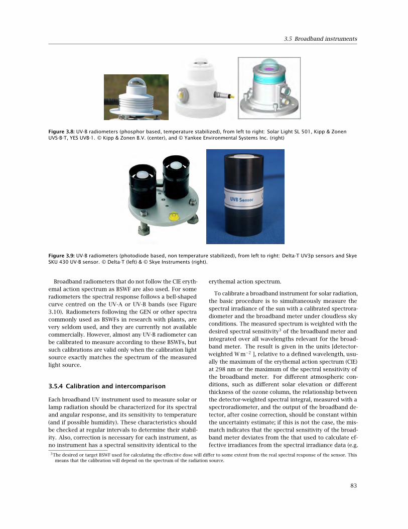
3.5 Broadband instruments

Figure 3.8: UV-B radiometers (phosphor based, temperature stabilized), from left to right: Solar Light SL 501, Kipp & ZonenUVS-B-T, YES UVB-1. © Kipp & Zonen B.V. (center), and © Yankee Environmental Systems Inc. (right)

Figure 3.9: UV-B radiometers (photodiode based, non temperature stabilized), from left to right: Delta-T UV3p sensors and SkyeSKU 430 UV-B sensor. © Delta-T (left) & © Skye Instruments (right).

Broadband radiometers that do not follow the CIE eryth-emal action spectrum as BSWF are also used. For someradiometers the spectral response follows a bell-shapedcurve centred on the UV-A or UV-B bands (see Figure3.10). Radiometers following the GEN or other spectracommonly used as BSWFs in research with plants, arevery seldom used, and they are currently not availablecommercially. However, almost any UV-B radiometer canbe calibrated to measure according to these BSWFs, butsuch calibrations are valid only when the calibration lightsource exactly matches the spectrum of the measuredlight source.

3.5.4 Calibration and intercomparison

Each broadband UV instrument used to measure solar orlamp radiation should be characterized for its spectraland angular response, and its sensitivity to temperature(and if possible humidity). These characteristics shouldbe checked at regular intervals to determine their stabil-ity. Also, correction is necessary for each instrument, asno instrument has a spectral sensitivity identical to the

erythemal action spectrum.

To calibrate a broadband instrument for solar radiation,the basic procedure is to simultaneously measure thespectral irradiance of the sun with a calibrated spectrora-diometer and the broadband meter under cloudless skyconditions. The measured spectrum is weighted with thedesired spectral sensitivity3 of the broadband meter andintegrated over all wavelengths relevant for the broad-band meter. The result is given in the units [detector-weighted W m−2 ], relative to a defined wavelength, usu-ally the maximum of the erythemal action spectrum (CIE)at 298 nm or the maximum of the spectral sensitivity ofthe broadband meter. For different atmospheric con-ditions, such as different solar elevation or differentthickness of the ozone column, the relationship betweenthe detector-weighted spectral integral, measured with aspectroradiometer, and the output of the broadband de-tector, after cosine correction, should be constant withinthe uncertainty estimate; if this is not the case, the mis-match indicates that the spectral sensitivity of the broad-band meter deviates from the that used to calculate ef-fective irradiances from the spectral irradiance data (e.g.

3The desired or target BSWF used for calculating the effective dose will differ to some extent from the real spectral response of the sensor. Thismeans that the calibration will depend on the spectrum of the radiation source.

83

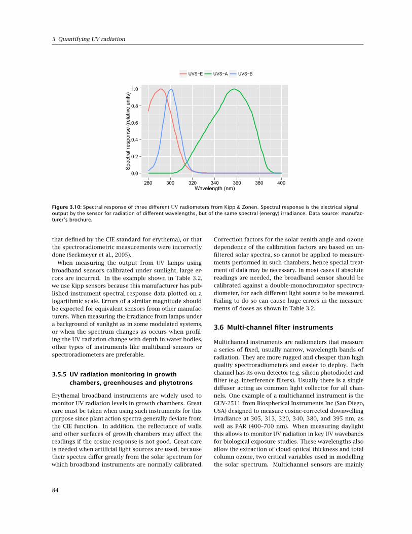
3 Quantifying UV radiation

0.0

0.2

0.4

0.6

0.8

1.0

280 300 320 340 360 380 400Wavelength (nm)

Spe

ctra

l res

pons

e (r

elat

ive

units

)

UVS−E UVS−A UVS−B

Figure 3.10: Spectral response of three different UV radiometers from Kipp & Zonen. Spectral response is the electrical signaloutput by the sensor for radiation of different wavelengths, but of the same spectral (energy) irradiance. Data source: manufac-turer’s brochure.

that defined by the CIE standard for erythema), or thatthe spectroradiometric measurements were incorrectlydone (Seckmeyer et al., 2005).

When measuring the output from UV lamps usingbroadband sensors calibrated under sunlight, large er-rors are incurred. In the example shown in Table 3.2,we use Kipp sensors because this manufacturer has pub-lished instrument spectral response data plotted on alogarithmic scale. Errors of a similar magnitude shouldbe expected for equivalent sensors from other manufac-turers. When measuring the irradiance from lamps undera background of sunlight as in some modulated systems,or when the spectrum changes as occurs when profil-ing the UV radiation change with depth in water bodies,other types of instruments like multiband sensors orspectroradiometers are preferable.

3.5.5 UV radiation monitoring in growthchambers, greenhouses and phytotrons

Erythemal broadband instruments are widely used tomonitor UV radiation levels in growth chambers. Greatcare must be taken when using such instruments for thispurpose since plant action spectra generally deviate fromthe CIE function. In addition, the reflectance of wallsand other surfaces of growth chambers may affect thereadings if the cosine response is not good. Great careis needed when artificial light sources are used, becausetheir spectra differ greatly from the solar spectrum forwhich broadband instruments are normally calibrated.

Correction factors for the solar zenith angle and ozonedependence of the calibration factors are based on un-filtered solar spectra, so cannot be applied to measure-ments performed in such chambers, hence special treat-ment of data may be necessary. In most cases if absolutereadings are needed, the broadband sensor should becalibrated against a double-monochromator spectrora-diometer, for each different light source to be measured.Failing to do so can cause huge errors in the measure-ments of doses as shown in Table 3.2.

3.6 Multi-channel filter instruments

Multichannel instruments are radiometers that measurea series of fixed, usually narrow, wavelength bands ofradiation. They are more rugged and cheaper than highquality spectroradiometers and easier to deploy. Eachchannel has its own detector (e.g. silicon photodiode) andfilter (e.g. interference filters). Usually there is a singlediffuser acting as common light collector for all chan-nels. One example of a multichannel instrument is theGUV-2511 from Biospherical Instruments Inc (San Diego,USA) designed to measure cosine-corrected downwellingirradiance at 305, 313, 320, 340, 380, and 395 nm, aswell as PAR (400–700 nm). When measuring daylightthis allows to monitor UV radiation in key UV wavebandsfor biological exposure studies. These wavelengths alsoallow the extraction of cloud optical thickness and totalcolumn ozone, two critical variables used in modellingthe solar spectrum. Multichannel sensors are mainly

84

3.7 Spectroradiometers

Table 3.2: Simulation of measured values for three common types of sensor. We simulate a perfect calibration for sunlight, andexpress the ‘measured’ irradiance by the sensors as a fraction of the true irradiance. We do this for some commonly-used lamptypes. We compare three types of lamps, UVB-313 and UVA-340 (Q-Panel) and TL12 (Philips) not filtered, and UVB-313 filteredwith cellulose di-acetate, in combination with three types of broadband sensors UVS-E (erythemal), UVS-A (unweighted UV-A), andUVS-B (unweighted UVB) from Kipp & Zonen (see Figure 3.10 for the sensor response spectra used). The sunlight spectrum used forcalibration is a daily accumulated value simulated for Jokioinen, Finland, for 21 May, expressed on an energy basis (see Kotilainenet al., 2011, for details). All spectra are simulated for clear sky conditions (CMF=1.0).

day 8:30 11:30 UVA-340 UVB-313 + acet. TL12 BSWF or wavelength band

UVS-E 1.00 1.03 0.95 0.77 0.42 0.47 0.37 CIE98, erythemalUVS-A 1.00 1.00 1.00 1.26 0.93 0.94 0.92 unweighted UV-A energy irradianceUVS-B 1.00 0.99 0.99 1.02 1.34 1.34 1.30 unweighted UV-B energy irradianceUVS-A 1.00 1.00 1.00 1.32 1.02 1.03 1.01 unweighted UV-A photon irradianceUVS-B 1.00 0.99 1.00 1.02 1.37 1.36 1.34 unweighted UV-B photon irradiance

used for long-term monitoring of UV irradiance and itsgeographic variation. They are also used for groundmeasurements used to calibrate space-borne instrumentscarried by satellites.

Recent multichannel instruments from BiosphericalInstruments are modular. They are composed of microra-diometers of small size, one for each channel, whichtogether with input optics and filters are used to buildthe multichannel instruments. Figure 3.11

The ELDONET terrestrial dosimeter consists of threebroad band sensors, measuring UV-B, UV-A and PAR irra-diance (Figure 3.12). It uses an integrating sphere to col-lect the light, which reaches the detectors after bouncingon the sphere walls. The autonomous version includesa built-in datalogger. It is waterproof, but it is not sub-mersible. The underwater version is described in section3.8.3 on page 95.

3.7 Spectroradiometers

Spectroradiometers4 are instruments used to measurespectral irradiance. There are two types of spectrora-diometer: 1) scanning spectroradiometers, and 2) arraydetector spectroradiometers. The former have a singlesensor, which is used to sequentially measure the spectralirradiance at each wavelength, while the latter have anarray of sensors onto which the refracted spectrum is pro-jected and measured simultaneously at all wavelengths.Sometimes the more general term spectrometer is ad-opted to indicate that the same instrument can be alsoused to measure spectral absorbance, -transmittance, or-reflectance, in addition to spectral irradiance. Scanningspectroradiometers scan a range of wavelengths. To dothis they require mechanically moving parts inside theoptic path and therefore need very stable housing for theinstrument. For this reason, scanning spectroradiometersare larger and more difficult to transport than array de-

tector spectroradiometers. They are also less rugged andusually require mains power. However, in scanning spec-troradiometers it is possible to use a double monochro-mator arrangement that makes their optical performancefar superior to that of array spectroradiometers whichalways use a single monochromator.

3.7.1 Scanning spectroradiometers

3.7.1.1 Basic structure and principles of operation

The basic components of a scanning spectroradiometerare the following: a) input optics for collecting radiationfrom the sky and guiding it further into the spectrora-diometer b) a monochromator for resolving the inputradiation into separate wavelengths c) a photomultipliertube (PMT) for detecting the energy possessed by eachspectral component in the measured spectrum. In addi-tion, an external computer for communication with themicroprocessor of the spectroradiometer and for collec-tion, processing and storage of data is needed.

The input optics typically consists of a flat teflon dif-fuser covered by a quartz dome. The diffuser collectsthe incident photons from the overhead hemisphere. Theresulting diffuse radiation is guided to the entrance slitof the monochromator, sometimes by means of an op-tical fibre. The monochromator may be a single or adouble monochromator (see section 2.2.4 on page 44). Inscanning spectroradiometers, a system based on a stepmotor drives a mask that allows only photons of a certainwavelength at a time to enter the exit slit of the mono-chromator. The exit slit serves as the entrance window tothe cathode of the PMT. The photon pulses are amplifiedand transmitted to a photon counter for registration.

Some spectroradiometers are constructed on a solartracker that follows the position of the sun. This elim-inates the effects of potential azimuthal dependenciesin the detection of radiation. A measurement head at

4It is necessary to distinguish between different types of instruments used to measure spectra or spectrometers. A spectrophotometer is aninstrument used to measure optical properties of objects while a spectroradiometer is used to measure radiation.

85

3 Quantifying UV radiation

Figure 3.11: Top: microradiometer used in multichannel instruments from Biospherical Instruments; bottom: radiance fore-opticsof a PRR-800 radiometer with 19 channels. Photographs © by Biospherical Instruments Inc.

Figure 3.12: ELDONET terrestrial dosimeter. (Photograph by Donat Häder, reproduced with permission.)

86

3.7 Spectroradiometers

the end of an optical fibre may be also installed on aseparate sun tracker. The temperature of the instrumentis usually either stabilized or kept above a certain tem-perature limit to ensure proper functioning. The domeof the measurement head may be equipped with a heaterand/or air blower to keep the temperature of the teflonwithin certain limits and to avoid emergence of frost ontothe dome.

Other spectroradiometers are less rugged and are in-tended for laboratory or spot measurements outdoors.They are more portable but more sensitive to temperat-ure extremes and are not water proof. Examples of suchinstruments are Optronics OL 756 and Macam SR9910spectroradiometers. Figure 3.13 shows the different partsof the first of these instruments.

The more rugged instruments, usually permanentlyinstalled at a fixed location, are commonly used for meas-uring long (several years long) time series of UV spectralirradiance data. The more portable instruments are usedfor spot measurements in plant canopies, and underlamps, and or filters. The first type of instrument is mostcommonly used by meteorologists, while the portableinstruments are most useful to biologists.

3.7.1.2 Characteristics

Dark current and dead time are characteristics pos-sessed by the PMT. Dark current is a measure of the driftphotons going from the cathode to the anode of the PMTwithout any real incident photons entering the instru-ment. Dead time is a measure of that PMT which is in aparalysed state after a photon detection event. Stray lightis composed of photons echoed from wavelengths otherthan the nominal wavelength being measured. In com-mercially available scanning spectroradiometers, thesephenomena are usually measured and handled by themeasurement software.

The wavelength alignment of a spectroradiometer hasto be checked regularly. Most instruments taking dailymeasurements contain an internal mercury lamp aimedat ensuring the stability of the alignment. The wavelengthand the position of the micrometer turning the gratingof the monochromator are related to each other by asecond-order equation using so called dispersion coeffi-cients. The determination of the dispersion coefficientsshould be part of the annual maintenance of the instru-ments.

Solar irradiance spectra sometimes exhibit so callednoise spikes, which mean sudden abnormally high orlow intensity readings on a single wavelength. The originof the spikes is not fully resolved, but straylight is con-sidered a partial explanation. The spikes can be detectedand eliminated making use of suitable reference spectra.

Ideally, the angular response of the measurement headfollows the shape of a cosine curve. In practice, theresponse deviates somewhat from this. Typically, the lar-ger the solar zenith angle, the larger the deviation. Thecosine response of the measurement head should bemeasured in laboratory and a corresponding correctionapplied to all measured data.

If the spectroradiometer is not stabilized for temperat-ure, its response usually exhibits temperature depend-ence. This dependence should be determined in thelaboratory by measuring a calibration lamp with a spec-troradiometer heated/cooled over a range of differentwavelengths. The measurements can be used for derivingthe temperature correction factors to be applied in thepost-processing of the sky measurements.

The slit function determines the transmittance of amonochromator as a function wavelength. The idealshape of the function would be triangular. The full widthat half maximum of the slit function is commonly usedas a quantity characterizing the slit function. The slitfunction can be derived by measuring the irradiance emit-ted by a tunable laser. Removal of the effect of the slitfunction on the measured spectra should be consideredif spectra measured by two or several instruments are tobe compared with each other.

The spectral responsivity of a spectroradiometershould be based on regular measurements of a certi-fied calibration lamp. If the responsivity seems to havechanged, basically two alternative ways to handle thechange exist. The change may be introduced in the re-sponsivity of the instrument and the processing of thesky measurements as such. A step-wise change in re-sponse is hence introduced in the time series of the meas-urements. Alternatively, a gradually changing responsetime-series may be defined using a moving average witha suitable time window. In this way, the change in theresponse is introduced gradually in the time series of thesky irradiance measurements.

3.7.1.3 Maintenance

The maintenance of a scanning spectroradiometer oper-ating in an outdoor environment involves the followingpractices: a) general daily maintenance; b) checks on thewavelength setting and stability of irradiance scale; c)calibration of irradiance against primary standards in adark room.

Daily routine maintenance includes cleaning of thequartz dome and checking on the general functioningas well as the correct levelling of the instrument. Thequartz dome should also be cleaned/dried after rain orsnow. The operator should be familiar with the controlsoftware of the instrument. Additional simple routinesbased on, for instance, selected reference spectra may be

87

3 Quantifying UV radiation

Figure 3.13: Diagram of a double monochromator scanning spectroradiometer, OL 756 from Gooch & Housego, Orlando, Florida,USA. Diagram © Gooch & Housego.

used for instant checking of the measured data. Thesekinds of routines are invaluable in the prompt detectionof occasional malfunctions of the instrument.

An internal Hg lamp is used for checking of thewavelength scale in some spectroradiometers. In thesecases, it is convenient to imbed the Hg lamp measure-ment into the daily measurement schedule. If the instru-ment lacks an internal lamp, this check has to be doneusing an external lamp. For checking the stability ofthe irradiance scale, portable calibration units are avail-able. These enable, for instance, stability checks of theinstrument at the measuring site on a weekly basis. It isadvisable that the humidity indicators are also checkedon a weekly basis.

Irradiance calibration of a spectroradiometer shouldbe performed in a dark room (Figure 3.14). A primarystandard lamp with an irradiance certificate provided bya certified laboratory of standards is needed. To extendthe lifetime of the primary standard lamp, it is recom-mended that it is not used as a regular calibration lamp.Instead, the irradiance scale of the primary lamp shouldbe transferred to a secondary standard lamp that is usedas a working calibration lamp. Use of several workinglamps is recommended to enable recognition of potentialdrifts in the radiant output of the lamps as they age. Cal-ibration against the primary/secondary standard lampshould be performed at least every two months. The de-siccant bags inside the cover of the spectrometer shouldbe taken out and dried at least every two months as well.

Proper levelling of the instrument has to be ensured afterhaving it relocated for outdoor measurements.

On the annual maintenance practices of a spectrora-diometer, each manufacturer has its own services andrecommendations. Participation in intercomparison cam-paigns gathering a number of state-of-the-art instrumentsto conduct measurements on a jointly agreed schedulefor a period of time has proven a fruitful way to investig-ate the long-term stabilities and overall performances ofscanning spectroradiometers (Figure 3.15).

3.7.2 Array detector spectroradiometers

In contrast to scanning spectroradiometers, array de-tector instruments measure spectral irradiance simul-taneously at all wavelengths. The detector in this caseis a linear array of light sensors, similar in structure tothe imaging sensors used in digital cameras, but longand narrow. The number of detector elements (‘pixels’)along the array varies, 2000 to 3000 pixels being com-mon5. The array can be a ‘charge coupled device’ (CCD),or an array of photodiodes (DAD). The ‘image’ of thespectrum produced by the monochromator is projectedand focused by means of mirrors onto the linear detectorarray, each detector in the array receiving light of a cer-tain wavelength. In the case of array spectrometers it isnot possible to use two monochromators in tandem toreduce stray light. Array spectrometers are small andportable (Figure 3.16).

5Some instruments with approximately 200 pixel arrays are also available, but these are usually called ‘hyperspectral radiometers’ instead ofspectroradiometers.

88

3.7 Spectroradiometers

Figure 3.14: Brewer#107 of the Finnish Meteorological Institute in the dark room of Jokioinen Observatory (on the left); a 1000Wcalibration lamp (on the right). Photograph: Anu Heikkilä.

Figure 3.15: Brewer spectroradiometers participating in a measurement campaign in Huelva, Spain, in October 2005. Photograph:Anu Heikkilä.

Figure 3.16: Left: Maya 2000 PRO spectrometer. Right: The same instrument connected to an optical fibre and a small cosinediffuser. Spectrometer and accessories from Ocean Optics. Photographs: Pedro J. Aphalo.

89

3 Quantifying UV radiation

For measuring energy or photon spectral irradiancea cosine diffuser is used as input optics. This ensuresthat the angular response follows the cosine law, andso the instrument measures the radiation as receivedon a flat surface. Other input optics are also available,for example, with a narrow angle of view. However, thequantity measured with them is not irradiance. Cosinediffusers differ widely in how closely they follow the co-sine law. Some cheaper models are prone to large errors,especially when radiation impinges at a sharp angle totheir surface. This will be further discussed in section3.7.2.1 on page 91.

The input optics is usually connected to the array spec-trometer with an optical fibre. The type of fibre to beused depends on the wavelength range to be measured.If smaller than the entrance of the spectroradiometer,the diameter of the fibre will affect the amount of ra-diation entering the instrument. The diameter also af-fects the mechanical properties of the fibre: thin fibresare more flexible and tolerate bending into curves ofsmaller diameter. Fibres also vary with regards to thetype of cladding material used to protect them. Fibreswith metal cladding tolerate rougher handling than thosewith plastic cladding. The most common connector forthese fibres and accessories is the SMA 905, originallydesigned for light fibres used in digital communicationsystems. For this reason their positioning upon repeatedattachment is not exactly the same. Consequently, therecommendation is not to detach and reattach the fibrefrom the spectrometer without recalibrating the system6.

At the entrance of the spectrometer, just behind theconnector to which the fibre is attached, there is a slit(Figure 3.17), which limits the width and height of theincoming light beam. The width is of the order of afew micrometres and the exact value chosen determines,together with the monochromator, the spectral resolu-tion of the spectroradiometer. The narrower the slit, thenarrower the beam hitting the monochromator and thebetter the resolution (the narrower the peaks that canbe resolved). In a Czerny-Turner configuration (Figure3.18), the next component is a collimating mirror whichprojects the beam onto a monochromator. Gratings areused as monochromators. Gratings have a surface withvery closely spaced rulings of a specific profile, and theyseparate radiation of different wavelengths in a similarway to a prism. One important parameter is the densityof rulings which is one of the determinants of spectralresolution and useful wavelength range. The ‘image’ pro-duced by the grating is focused onto the array detectorby another collimating mirror. Some newer models ofspectrometer from StellarNet (e.g. BLACK-Comet spec-

trometer) and now also from Ocean Optics (Torus spec-trometer) use a concave grating instead of a planar one.Since the grating itself focuses the light onto the array de-tector, collimating mirrors are not needed. Having feweroptical components, an instrument with better stray lightperformance is obtained.

The array detector normally has rectangular ‘pixels’,orientated so that their shorter dimension is on the axisalong which the different wavelengths have been separ-ated by the monochromator, and their longer dimensionis perpendicular to it. The entrance slit is positionedto have the long dimension coincident with the long di-mension of the pixels. In some detectors the long pixelsare in reality rows of square pixels with their electricaloutput combined into a single output signal. The out-put signal from the pixels is averaged by the detectoritself over what is called ‘integration time’. The longerthe integration used, the lower the irradiance that can bemeasured. However, the ‘dark noise’ increases with theintegration time. In addition, it is possible to take severalscans and average them. A coarse dark noise correctionis sometimes done by subtracting the signal from specialpixels at the end of the array that are not exposed toradiation. However a dark scan, with the input opticsprotected from the incoming radiation, should also bemeasured, and its value, wavelength by wavelength sub-tracted from the measurements. The dark noise dependson temperature. This has two implications, dark scansshould be taken frequently, sometimes before or aftereach measurement, and the spectrometer should be al-lowed to warm up for some minutes before starting totake readings. Furthermore, when working outdoors itshould be protected from direct sunlight, so as to keep itstemperature stable and close to that at which it was cal-ibrated. Some spectrometers have a thermoelement (TE),working according to the Peltier principle, which coolsthe array detector to a preset temperature and therebystabilizes it.

Most current array spectrometers, the exception beingsome models with thermoelectrically cooled detectors,are powered through the USB port of a personal computer.For portable use a laptop is frequently used. Special soft-ware, sold by the manufacturer of the spectrometer, isused to control the instrument and acquire and plot thespectra (Figure 3.19). For most instruments there arealso drivers and software development kits (SDK) avail-able for developing programs for special applications.When special corrections, for example for stray light, areperformed it may be necessary to acquire raw spectraldata and apply corrections and calibrations off-line usingother software, for example Excel or R.

6Errors caused by detaching and reattaching a fibre with an SMA connector can be ±5% (Nevas et al., 2012), but the information available is ratherlimited, so if the fibre is going to be detached, the errors should be characterized for each individual instrument. Errors caused by attaching andreattaching a fibre with an FC connector are negligible (Nevas et al., 2012)

90

3.7 Spectroradiometers

Figure 3.17: Left: A CCD array detector with an order sorting filter applied; right: the slit of an AvaSpec spectrometer. Photo-graphs, Left: © Ocean Optics; right: © Avantes.

1

6

3 25

4

7

Figure 3.18: Two different layouts for the optical bench of array spectrometers. At the top a symmetrical Czerny-Turner config-uration exemplified by the AvaBench used in most Avantes instruments, and at the bottom a Czerny-Turner configuration with acrossed light pass as used in the Ocean Optics USB4000 spectrometer. [1] SMA connector, [2] entrance slit, [3] optional filter, [4]collimating mirror, [5] grating, [6] focusing mirror, [7] detector. Top figure, © Avantes; bottom figure, © Ocean Optics.

3.7.2.1 Measuring errors and limitations in accuracy

Array spectroradiometers have a great advantage whenquickly measuring changing radiation as they acquire allwavelengths simultaneously. This ensures that the valuesof spectral irradiance measured at all wavelengths areconsistent. In contrast, under conditions where irradi-ance varies rapidly with time, the shape of the measuredspectrum can get badly distorted when measured witha scanning spectroradiometer. However, array spectro-meters have a serious limitation in that they cannot bebuilt with double monochromators. As any spectrora-diometer with a single monochromator, they suffer fromrelatively high values of stray light. Stray light originates

from scattered light of incorrect wavelengths falling on apixel of the array detector. In other words, radiation ofone wavelength is detected (and measured) as radiationof a different wavelength. Perfectly scattered radiationwould affect all pixels in the same way, but when thereare reflections within the optical bench that are not per-fectly scattered, some pixels in the array detector aremore affected by stray light than others. Stray light is acritical specification when measuring UV-B in sunlight, asUV-B irradiance is very low compared to the irradianceof visible and near infra-red radiation. Consequently, ifeven a small proportion of visible radiation is scatteredand reflected as stray light within the instrument, thisstray light can generate a signal on the ‘UV-B pixels’ of

91

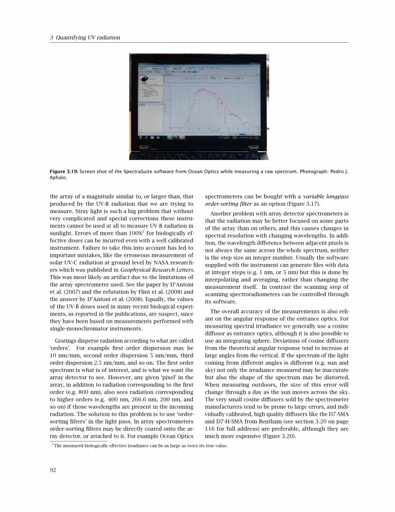
3 Quantifying UV radiation

Figure 3.19: Screen shot of the SpectraSuite software from Ocean Optics while measuring a raw spectrum. Photograph: Pedro J.Aphalo.

the array of a magnitude similar to, or larger than, thatproduced by the UV-B radiation that we are trying tomeasure. Stray light is such a big problem that withoutvery complicated and special corrections these instru-ments cannot be used at all to measure UV-B radiation insunlight. Errors of more than 100%7 for biologically ef-fective doses can be incurred even with a well calibratedinstrument. Failure to take this into account has led toimportant mistakes, like the erroneous measurement ofsolar UV-C radiation at ground level by NASA research-ers which was published in Geophysical Research Letters.This was most likely an artifact due to the limitations ofthe array spectrometer used. See the paper by D’Antoniet al. (2007) and the refutation by Flint et al. (2008) andthe answer by D’Antoni et al. (2008). Equally, the valuesof the UV-B doses used in many recent biological experi-ments, as reported in the publications, are suspect, sincethey have been based on measurements performed withsingle-monochromator instruments.

Gratings disperse radiation according to what are called‘orders’. For example first order dispersion may be10 nm/mm, second order dispersion 5 nm/mm, thirdorder dispersion 2.5 nm/mm, and so on. The first orderspectrum is what is of interest, and is what we want thearray detector to see. However, any given ‘pixel’ in thearray, in addition to radiation corresponding to the firstorder (e.g. 800 nm), also sees radiation correspondingto higher orders (e.g. 400 nm, 266.6 nm, 200 nm, andso on) if those wavelengths are present in the incomingradiation. The solution to this problem is to use ‘order-sorting filters’ in the light pass. In array spectrometersorder-sorting filters may be directly coated onto the ar-ray detector, or attached to it. For example Ocean Optics

spectrometers can be bought with a variable longpassorder-sorting filter as an option (Figure 3.17).

Another problem with array detector spectrometers isthat the radiation may be better focused on some partsof the array than on others, and this causes changes inspectral resolution with changing wavelengths. In addi-tion, the wavelength difference between adjacent pixels isnot always the same across the whole spectrum, neitheris the step size an integer number. Usually the softwaresupplied with the instrument can generate files with dataat integer steps (e.g. 1 nm, or 5 nm) but this is done byinterpolating and averaging, rather than changing themeasurement itself. In contrast the scanning step ofscanning spectroradiometers can be controlled throughits software.

The overall accuracy of the measurements is also reli-ant on the angular response of the entrance optics. Formeasuring spectral irradiance we generally use a cosinediffusor as entrance optics, although it is also possible touse an integrating sphere. Deviations of cosine diffusersfrom the theoretical angular response tend to increase atlarge angles from the vertical. If the spectrum of the lightcoming from different angles is different (e.g. sun andsky) not only the irradiance measured may be inaccuratebut also the shape of the spectrum may be distorted.When measuring outdoors, the size of this error willchange through a day as the sun moves across the sky.The very small cosine diffusers sold by the spectrometermanufacturers tend to be prone to large errors, and indi-vidually calibrated, high quality diffusers like the D7-SMAand D7-H-SMA from Bentham (see section 3.20 on page116 for full address) are preferable, although they aremuch more expensive (Figure 3.20).

7The measured biologically effective irradiance can be as large as twice its true value.

92

3.7 Spectroradiometers

Figure 3.20: Bentham D7-H-SMA cosine diffuser. Photograph: Pedro J. Aphalo.

3.7.2.2 Calibration and corrections

When measuring UV-B with an array spectroradiometerit is not enough to have it properly calibrated, its op-tical characteristics (slit function at different wavelengths,stray light properties) need to be measured and a cor-rection algorithm developed and later applied to eachmeasurement. This makes the use of array spectrora-diometers for characterizing UV-B doses complicated anderror prone. This type of use has to be attempted only byexperienced operators and the correction algorithm itselfrequires lots of effort to develop and implement. Giventhe lack of standardized procedures for stray light cor-rection, its implementation requires advanced knowledgeof optics and metrology. We will first discuss spectral cal-ibration and thereafter stray light correction procedures.

Spectral calibration against standard lamps needs to berepeated regularly. For measurements not requiring veryhigh precision, annual re-calibrations may be enough.However, the main consideration should be how valuableis the data that will be acquired. If the spectral sensit-ivity of the instrument has changed significantly fromone calibration to the next, the data from all measure-ments done in between these calibrations are suspect,and should be discarded. Consequently if one does yearlyre-calibrations one can lose one year’s worth of data,while if one does monthly re-calibrations one only riskslosing one month’s worth of data. Consequently, the de-cision on how frequently to calibrate should, in additionto instrument stability, be based on the maximum size ofthe tolerable errors and on the value of the data (i.e. thecost of replacing the data if they need to be discarded).

The most common and stable calibration light sourcesare incandescent lamps (e.g. FEL lamps) with electronicsin the power source which keeps the electrical power atthe filament constant within very narrow margins. Thedistance between the lamp and the entrance optics, andtheir alignment, should also fall within a very narrowmargin of the expected values. Calibration lamps aresecondary or tertiary standards, connected by a chain of

calibration steps to a standard kept at a metrology agencylike NIST. Calibration lamps are supplied with spectraldata about their emission characteristics. Calibration ofthe instrument is done by measuring the known spec-trum and irradiance of the calibration lamp. Of coursethe output of the lamp will not exactly match the datasupplied with it, because its original calibration is alsosubject to errors. Furthermore, there are errors derivingfrom slight differences between the burning conditions(current and voltage) during measurements and thosewhen it was calibrated at the factory. Further errors canbe introduced by small differences in the geometry ofthe optical setup. So, do not forget that calibrations aresubject to errors. Furthermore, you cannot obtain anabsolute estimate of calibration errors by comparing twoinstruments calibrated with the same lamp, unless thislamp is the primary standard.

Calibrating a spectroradiometer in the UV-B band witha FEL lamp is not recommended, because FEL lamps emitvery little UV-B. For calibration in the UV-B deuteriumlamps need to be used. Irradiance emitted by deuteriumlamps is less stable than that emitted by FEL lamps. Forcoarse calibration the use of a deuterium lamp may beenough, but for accurate calibration it is best to use FELand deuterium lamps in tandem. The shape of the spec-trum emitted by deuterium lamps is stable, by matchingthe irradiances at wavelengths where the emission ofboth types of lamps overlap, one can extend an accuratecalibration to shorter wavelengths. Spectrometer man-ufacturers also sell calibration light sources (lamp pluselectronics) that may be good for routine calibration orespecially for checking that calibrations performed inan optical bench remain valid. Again, what type of cal-ibration procedure and lamp to use will depend on theaccuracy required. If we want our measurements to bewithin ±10% of the true value we will need to use verygood equipment and protocols for the calibration. If wecan tolerate errors of, for example, ±25%, calibrationscan be less accurate.

93

3 Quantifying UV radiation

It is also very important to do a wavelength calibra-tion and to check this calibration regularly. It shouldnot be forgotten when doing this calibration that it isaffected by the temperature of the instrument as tem-perature affects (by thermal expansion) the dimensionsof the optical bench and its components. Wavelengthcalibration is done based on elemental emission linesin discharge lamps (or even the sun). For quick checkslow pressure mercury or germicidal lamps may be used.The manufacturers of spectrometers also sell speciallight sources for wavelength calibration. One shouldchoose carefully which wavelengths to use (for example253.652 nm, 296.728 nm, 334.148 nm, and 404.657 nmfor mercury lamps, as they are simple peaks rather thanmultiple peaks very close together like those at 302 nm,313 nm and 365 nm). If one desires a calibration accur-ate to a fraction of the wavelength step of the array oneneeds to fit a bell-shaped curve to the pixel showing thehighest signal and those adjacent to it, to find the truelocation of the peak centre, most likely in-between twopixels.

To keep errors within ±10% in the UV-B when measur-ing sunlight, and especially to keep errors within ±10%for biologically effective doses, a good calibration is notenough when using single monochromator spectrora-diometers. There is also a need to correct for stray light.If we do not correct for stray light some biologically ef-fective doses will be overestimated by more than 100%.The ratio between stray light in the UV-B band and themaximum spectral irradiance measured in good singlemonochromator spectrometers is approximately 1×10−3,while in double monochromator spectroradiometers itcan be as low as 1× 10−6. If time for scanning, cost andlack of portability are no obstacles, it’s preferable to usedouble monochromator instruments and these shouldalso be used as the main instrument in a laboratory.

When applying the stray light correction, a thor-ough characterization of the slit function at differentwavelengths and a check of the wavelength dependenceof stray light are needed. This characterization doesnot need to be repeated, unless changes are made tothe optical bench of the instrument. So, in contrast tothe spectral calibration, the stray light characterizationneeds to be performed only once during the lifetime ofthe instrument unless major repairs or modifications aremade.

In some array spectrometers, depending on the config-uration, the width of the slit function may vary with thewavelength. This can introduce errors that are very diffi-cult to correct. In some cases it might be preferable tochose a grating giving the instrument a relatively narrowwavelength range, for example 250 nm to 500 nm if theintended use is to measure UV irradiance.

The use and calibration of array spectroradiometers formeasurement of UV-B radiation in sunlight is discussedin detail in the WMO report by Seckmeyer, Bais, Bernhard,Blumthaler, Drüke et al. (2010). Stray light correctionmethods are discussed in the papers by Ylianttila et al.(2005), Coleman et al. (2008), and Kreuter and Blumthaler(2009) and the references therein.

3.8 Underwater sensors and profiling

3.8.1 Measuring underwater UV radiation

Measuring UV radiation in the aquatic environment isdifficult. Waterproof UV-measuring devices are neededor sensors protected in water proof housings as well asa means of deploying the sensors at the desired depth.Frequently, underwater measurements are referenced tothe (spectral) irradiance at the surface of the water body,measured simultaneously with a matched “atmospheric”or terrestrial sensor.

As was mentioned in section 1.6 on page 15, measure-ment of the underwater UV field presents particular com-plexities, mainly related to variable attenuation occurringin different water bodies (Kirk, 1994a). Depending on thephysical and chemical characteristics of the water, UV ir-radiance may decrease much more rapidly than PAR irra-diance (this phenomenon is known as ‘spectral leakage’),resulting in a changing spectrum with depth. Thus, un-derwater UV instruments are normally equipped with dif-ferent filters and photodiodes to minimize these effectsand to improve the sensitivity to particular wavelengthsof interest. As discussed above in section 3.5.4 on page83, errors are introduced if the spectrum being measureddiffers from that of the source used for calibration ofthe broadband instrument. This implies that when usingbroadband sensors underwater the errors will depend onthe depth at which the radiation is being measured. Inaddition, a general problem exists for broadband sensorsand spectrometers if sensors are only calibrated in air.The same calibration function cannot be used with thesensor in air and in water. Wavelength-dependent correc-tion factors, so called immersion factors, must be usedto adjust the signal if sensors are immersed in water asfor example described by Ohde and Siegel, 2003.

Water movement and weather conditions can affect themeasurements of underwater UV radiation. For an ac-curate determination of UV radiation in the field, sunny,cloudless conditions and calm waters are preferred. Theeffect of waves may cause difficulties especially whenmeasuring near the surface. On the other hand, cloudsand other atmospheric UV absorbing phenomena can al-ter the conditions during the measurement of verticallight profiles, especially when the diffuse component of

94

3.8 Underwater sensors and profiling

the beam is altered.Solar zenith angle is an important factor which affects

the irradiance above the water surface, and also the re-flectance of the water surface for the wavelengths ofbiological relevance. In addition, the radiation amplific-ation factor (RAF, see also section 3.10), can be used toestimate the effect of changes in the ozone column onbiologically effective exposure. Corrections can be ap-plied to measurements performed with broadband instru-ments, but measurements with narrow-band multi-filterinstruments and spectroradiometers are less error prone.

If our objective is to describe the characteristics of thewaters, UV radiation should be measured around solarnoon, when solar elevation is maximal. However, if we areinterested in describing the daily UV exposure of some or-ganism, measurements should be done preferably duringmost of the day and at the depths of interest.

3.8.2 Profiling

Profiling is the measurement of irradiance or spectralirradiance as a function of depth in a water body. Specialframes are used for lowering the instruments throughthe water. For light measuring instruments, the frame orrig should not occlude the field of view of the radiationsensors. A means of determining the depth at which thesensor is located, and any deviation from a vertical ori-entation should also be available. Suitable cabling is usedto connect the underwater sensors to onboard computersor dataloggers.

3.8.3 Underwater radiometers

Various underwater radiometers are currently availableand their accuracy and characteristics vary consider-ably. The most appropriate instrument to choose de-pends on the specific goals of a study. Different typesof radiometers include broadband radiometers, narrow-band multifilter radiometers, photodiode array spectrora-diometers, and scanning spectroradiometers, includingsingle monochromator spectroradiometers. Comparisonsof the main characteristics of different types of instru-ments have been published (S. B. Díaz et al., 2000; Kirk,1994a; Kjeldstad et al., 2003; Tedetti and Sempére, 2006).Some commonly-used underwater UV instruments aredescribed below.

The ELDONET radiometers (Real Time Computer, Ger-many) were developed within the framework of theEuropean light dosimeter network (Figure 3.21) and havebeen described in detail (Häder et al., 1999). The dosi-meters are three-channel broadband filter devices withan entrance optic consisting of an integrating Ulbrichtsphere with an internal BaSO4 coating (Khanh and Dähn,1988). Silicon photodiodes (BPX60 for the PAR range and

SFH291 for the two UV wavebands, both from Siemens,Germany) are used in combination with custom-madefilters to select the wavelength ranges for UV-B (280-315 nm), UV-A (315-400 nm) and PAR (400-700 nm), acustom-made interference filter for UV-B (Janos Tech-nology, Townshend, VT, USA), a DUG 11 band filter forUV-A (Schott & Gen., Mainz, Germany) and a broad bandfilter for PAR (WBHM, Optical Coating Laboratory, SantaRosa, CA, USA). Eldonet performs 60 measurements eachminute.

Submergible multichannel radiometers like PUV 500,PUV 2500 series from Biospherical Instruments (SanDiego, USA) are equipped with narrow-band filter de-tectors in the range of UV and PAR (Figure 3.22). Theseradiometers are equipped with depth and temperaturesensors and thus are well suited for accurate light profil-ing. The spectral characteristics of the five filters used inthe PUV 500 instrument are as follows: 305±1 nm (bandpass 7±1 nm) 320±2 nm (band pass 11±1 nm) 340±2 nm(band pass 10±1 nm) 380±2 nm (band pass 10±1 nm)

On the other hand, the PUV 2500 measures 7 (option-ally 8) wavebands of downwelling irradiance (305, 313,320, 340, 380, 395 nm and PAR: 400–700 nm) with oneupwelling radiance channel (natural fluorescence). Eachchannel with 10 nm FWHHM except 305 (controlled byatmospheric ozone cutoff). The instrument includes pres-sure/depth sensing (350 m maximum) and temperaturecontrol. A 32 channel multiplexer selects signals from 8photodetectors, temperature, pressure and tilt/yaw de-tector. The cosine collector is made of Teflon-coveredquartz for use in the water.

The RAMSES family of hyperspectral radiometers(Trios GmbH, Germany) are miniature single monochro-mator spectrometers with a resolution of 2 to 3 nm perpixel and 100 or 190 usable channels in the photodiodearray (Figure 3.23). They can be used in air or in water.The Ramses ACC-UV is an integrated UV hyperspectral ra-diometer, and the Ramses ACC-VIS is a UV-A and visiblehyperspectral radiometer, both equipped with a cosinecollector. Ramses ASC-VIS is equipped with a sphericalcollector shielded so as to measure radiation from onehemisphere. To measure scalar irradiance, two of thesesensors can be deployed pointing in opposite directions.They are calibrated for underwater and air measurements(two different calibrations). The device has a small size,the signal capture requires some power consumption andportable (laptop) terminal at the surface. The detectortype is a silicon photodiode array designed to capturewavelengths between 320–950 nm for VIS models and280–500 nm for the UV models, with an irradiance accur-acy better than 6–10% depending on the spectral range.

Although the LI-1800UW instrument is not currentlyproduced by LI-COR, many foundational studies focused

95

3 Quantifying UV radiation

Figure 3.21: Underwater Eldonet (European light dosimeter network). (Photograph by Donat Häder, reproduced with permission.)

Figure 3.22: Biospherical PUV500 and PUV 510 (underwater). Left: © Biospherical Instruments, Right: Félix López Figueroa.

Figure 3.23: RAMSES-ACC-UV hyperspectral radiometer. © Trios GmbH.

96

3.9 Modelling

on UV penetration during the 1980s and 1990s werecarried out using this spectroradiometer. The opticsof this scanning spectroradiometer is based on a singleholographic monochromator grating, a silicon detectorand a filter wheel to improve stray light rejection. Thewavelength range is between 300 and 850 nm, with abandwidth of 8 nm and accuracy of ±1.5 nm. Originallyoptional slits of different widths were available, so thesespecifications vary with the exact configuration used. Thewhole optical bench and the microcomputer system iscontained in the massive waterproof housing designedfor measurements to a depth close to 200 m. Being asingle monochromator instruments its accuracy is lim-ited by stray light when used to measure UV-B radiationin daylight.

The OL 754-O-PMT Spectrometer Optics Head (OptronicLaboratories) is based on a double monochromator forlow stray light and measuring from 300 to 850 nm.Configurations with other gratings giving differentwavelength ranges are available. The system utilizes holo-graphic gratings with peak efficiencies at 300 nm. Theinstrument can be fitted with an OL IS-470-WP Submers-ible Sphere Assembly (4-inch integrating sphere) attachedby means of quartz optical fibre to the non-submersiblespectroradiometer. The sphere follows a dual port designwith an entrance port and an exit port located 90 apart.The sphere contains an internal baffle in front of the exitport to permit only light reflected by internal surface ofthe sphere to exit the sphere and enter the fibre.

Another approach to measuring underwater UV radi-ation is to protect a regular UV sensor, as for example,those described in section 3.5.2 on page 82, within a her-metic water-proof housing (Figure 3.24). Of course theenclosure should have an UV transparent window, andthe sensors must be calibrated inside the enclosure.

3.9 Modelling

For locations and times not covered by measurements,alternative approaches have to be considered for estim-ating the prevailing radiation conditions. For this pur-pose, various methods for modelling the surface UV ra-diation have been developed. These range from simpletheoretical-empirical methods for estimating the clear-sky surface radiation to more sophisticated methodsthat account also for the effects of clouds as inferredeither from ground-based station data or satellite meas-urements. Table 3.3 gives a simplified view of the mainfeatures of methods that are available for modelling thesurface UV radiation.

Simple theoretical-empirical methods, such as those ofBjörn and Murphy (1985) and Bird and Riordan (1986),have been widely used thanks to their fairly simple user

interface. These methods provide spectral surface irradi-ances, optionally on tilted surfaces, and account for themain parameters affecting the surface radiation condi-tions under cloudless skies. Results indicate that theypredict the surface radiation with reasonable accuracy ascompared to more detailed radiative transfer calculationsand measurements (Bird and Riordan, 1986).

Another user-friendly alternative is to use an inter-active web-based interface to radiative transfer sim-ulations, such as the FastRT (Engelsen and Kylling,2005, available at http : / / nadir . nilu .no / ~olaeng / fastrt / fastrt . html) orthe QUICK TUV (http://cprm.acd.ucar.edu/Models/TUV/Interactive_TUV/). Both of theseare based on rigourous radiative transfer models, whichmeans that their accuracy depends mainly on the choiceof values for the input parameters. Both include a se-lection of biological weighting functions, and FastRTalso provides the possibility to account for the effectof clouds.

When cloud effects need to be accounted for in detail,either satellite methods or so-called UV reconstructionmethods should be considered. The UV reconstructionmethods usually rely on ground-based measurements ofsome kind for accounting for the effect of clouds on radi-ation. Although the methods vary in their exact approach,the idea of all of them is to utilize available observationsto account for the parameters that affect the amount ofUV radiation reaching the surface. These parameters are,most importantly, clouds, total ozone column, surfacealbedo, atmospheric aerosols, and altitude or pressure.In addition, the solar zenith angle determines the pathlength of the direct radiation through the atmosphereand is therefore the single most important factor for thesurface UV radiation. The Earth-Sun distance, which var-ies over the course of the year, also needs to be accountedfor.

Many station-based methods for reconstructing thesurface UV radiation were included in recent Europeanefforts to gain a better understanding of past UV radi-ation and its climatological behaviour (den Outer et al.,2010; Koepke et al., 2006). Similar methods have beenproposed and applied in other parts of the world aswell (V. E. Fioletov et al., 2004; V. Fioletov et al., 2001).Compared to satellite methods, the advantage of thestation-based methods is that they tend to give moreaccurate estimates of the surface UV radiation. In partic-ular, methods using global solar radiation (300–3000 nm),measured by pyranometers at numerous stations world-wide, as input for determining the cloud effect typicallyshow small bias and fairly small scatter when comparedto measurements (Koepke et al., 2006). To mention oneexample, Lindfors et al. (2007) estimated daily erythemal

97

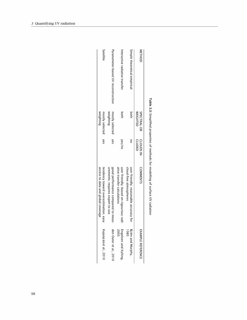
3 Quantifying UV radiation

Tab

le3

.3:Sim

plifi

edpro

perties

of

meth

ods

for

modellin

gof

surface

UV

radiatio

n

MET

HO

DSPEC

TR

AL

OR

WEIG

HT

EDC

LOU

DS

IN-

CLU

DED

CO

MM

ENT

SEX

AM

PLER

EFEREN

CE

Simple

theo

retical-empirical

both

no

user

friendly;

reasonab

leaccu

racyfo

rclo

ud-free

atmosp

heres

Bjö

rnan

dM

urp

hy,

19

85

Interactive

radiative

transfer

both

yes/no

user

friendly;

based

on

rigouro

us

radi-

ativetran

sfercalcu

lations

Engelsen

and

Kyllin

g,

20

05

Pyranom

eter-based

UV

reconstru

ction

mostly

selectedw

eightin

gyes

good

perfo

rman

ceco

mpared

tom

eas-urem

ents;

requires

expert

touse

den

Outer

etal.,

20

10

Satellitem

ostly

selectedw

eightin

gyes

tenden

cyto

ward

overestim

ation;easy

accessto

data

and

glo

bal

coverag

eK

ujan

pää

etal.,

20

10

98

3.10 BSWFs and effective UV doses

Figure 3.24: Hermetic water -proof housing without and with light sensors and data logger inside of the box. Photographs © EIC(Equipos, Instrumentación y Control).

UV doses at four Nordic stations, and found a systematicdifference of between 0 and 4%, depending on the station,and a root-mean-square error of 5–9% as compared tomeasurements for the summer period.

Satellite methods are based on radiative transfer sim-ulations combined with information on, for example,clouds and total ozone column retrieved from the satel-lite observations. Satellite retrieved UV irradiances typic-ally show an overestimation of 10% or more, and a largescatter, when compared to surface measurements: theroot-mean-square errors for daily erythemal UV dosestends to be of the order of 30–40% (Kujanpää et al., 2010;Lindfors, Tanskanen et al., 2009; Tanskanen et al., 2007).The main part of the overestimation is usually attributedto aerosol absorption, which is not accounted for prop-erly in current satellite UV algorithms. The advantageof satellite methods, on the other hand, is their largegeographical coverage, often global, and easy access todata that they provide.

Most methods, both station-based UV reconstructionmethods and satellite methods, only provide UV datacorresponding to a selection of weighting functions (e.g.,erythemally weighted UV), and, in addition, sometimesirradiances for selected wavelengths. Furthermore, themethods typically include only irradiances for a hori-zontal surface. This may become an obstacle for biolo-gical applications where, for example, a specific weightingfunction or spectral information would be preferred. Inprinciple, however, many of the methods could be exten-ded to produce spectral irradiances and fluence rates. Onthe other hand, fluence rates can also be estimated basedon the horizontal irradiance (e.g., Kylling et al., 2003).

Recently, Lindfors, Heikkilä et al. (2009) presented amethod for modelling spectral surface irradiances. Themethod relies on radiative transfer simulations, and takesas input (1) the effective cloud optical depth as inferredfrom pyranometer measurements of global radiation; (2)the total ozone column; (3) the surface albedo as estim-ated from measurements of snow depth; (4) the total

water vapour column; and (5) the altitude of the location.Figure 3.25 shows a comparison between the daily accu-mulated irradiances at 300 and 320 nm from this methodand measurements with a Brewer spectroradiometer atJokioinen, southern Finland. At both wavelengths, thereconstructed irradiances closely follow the measuredones.

A variety of methods for modelling the surface UVradiation are available. Which method is the best, orthe most appropraite, depends on the specific questionthat is to be answered. In general, the complexity of themethod tends to grow with increasing accuracy, and thepyranometer-based UV reconstruction methods, that areconsidered to provide highest accuracy, typically requirean expert user. The use of such a method will, how-ever, increase cross-disciplinary collaboration and maytherefore be worthwhile.

3.10 BSWFs and effective UV doses

The emission spectrum of UV-B lamps, even filtered withacetate, is different to that of the effect of ozone deple-tion. The spectrum of the effect of ozone depletion notonly changes with ozone column thickness, but also withsolar elevation. In other words, it changes through aday and with seasons (Figure 3.26). Because of this, it isalmost impossible to exactly simulate the effect of ozonedepletion in field experiments. The best we can do is tocalculate effective doses.

Biologically effective exposures (see Box 3.1) are a wayof measuring radiation differing in spectral compositionwith the same ‘measuring stick’. This ‘measuring stick’is a biological response. Behind each UV-BBE measure-ment we need to assume the involvement of a biologicalresponse. If we know the action spectrum for the bio-logical response, we can use it as a BSWF: We multiply,wavelength by wavelength the spectral irradiance of thelight source by the BSWF obtaining a weighted spectrum,giving a biologically-effective spectral irradiance (Figure

8Graphically this is the area under the curve.

99

3 Quantifying UV radiation

10

20

30

40

2000

4000

6000

8000

300 nm320 nm

100 200 300Julian day

Spe

ctra

l da

ily e

xpos

ure

( J m

−2 n

m−1

)

measured reconstructed

Figure 3.25: Reconstructed and measured daily cumulative irradiances at (a) 300 nm and (b) 320 nm at Jokioinen during 2004.From Lindfors, Heikkilä et al., 2009.

Box 3.1: Biologically effective irradiance: what is it, and what it is used for?

By ‘biologically effective irradiance’ we mean the irradiance weighted according to the effectiveness of differentwavelengths in eliciting a photobiological response. The most frequently used biologically effective irradiancequantities are photometric quantities such as those described in Box 1.1 on page 6. In the case of photometricquantities the (energy) irradiance is weighted according to the response of the human eye.When studying the effects of UV-B radiation on plants we use as biological spectral weighting functions (BSWFs)spectra describing the response of some plant function. For example an action spectrum for accumulation offlavonoids, or an action spectrum for growth inhibition. To be able to calculate biologically effective irradiancesusing any BSWF, we need to measure the spectral irradiance of the light source.If we integrate the effective irradiance for the duration of an experiment then we obtain a biologically effectiveexposure (usually called ‘biologically effective dose’ by biologists). If we do the time integration for one day weobtain a biologically effective daily exposure.These weighted irradiances are usually expressed using units corresponding to the underlying energy irradiances,independently of the BSWF used. Quantities calculated using different BSWFs are expressed in the same units, butthe values cannot be compared because in reality they are measured on different scales.

100

3.10 BSWFs and effective UV doses

04:30 11:30

0.00

0.01

0.02

0.03

0.04

0.05

280 320 360 400280 320 360 400Wavelength (nm)

Spe

ctra

l irra

dian

ce d

iffer

ence

and

lam

p irr

adia

nce

(rel

ativ

e en

ergy

uni

ts)

20% depleted ozone lamp

Figure 3.26: Comparison of spectral (energy) irradiance from Q-Panel UVB-313 lamps filtered with cellulose acetate film and theeffect of 20% ozone depletion on the solar spectrum at two times of the day. For details of the simulations see fig. 1.7. Spectralirradiances normalized to equal total UV energy irradiance (= area below the curves).

3.27). We then integrate the result over wavelengths, toobtain a single number, the biologically effective UV irra-diance8. In Figure 3.27 it also possible to appreciate thedifference in relative change of this effective irradiance,for a given level of ozone depletion, depending on theBSWF used.

It is important to make sure that both the irradianceand the effectiveness are measured using compatibleunits. It is common to express action spectra as spec-tral quantum effectiveness and to measure light sourcesas spectral (energy) irradiance. In UV research, biolo-gically effective doses are most frequently expressed inweighted energy units and to be able to calculate thesedoses from spectral (energy) irradiance measurementsfor a light source (sunlight or lamps) one needs to usean action spectrum expressed in energy effectiveness.Most common formulations of action spectra need to betransformed from quantum effectiveness to energy ef-fectiveness (one important exception is the CIE erythemalspectrum formulation). This is something that is oftenneglected, and is a source of difficulties when comparingdoses between different publications.

Another possibility for measuring effective doses is tohave a broadband sensor with a spectral response resem-bling the action spectrum of interest. In practice the spec-tral response of such sensors is only an approximationto the desired BSWF and consequently need to be calib-rated under the light source to be measured, usually bycomparison to a double monochromator scanning spec-troradiometer (see section 3.7 on page 85). Most such

sensors are calibrated for sunlight, and consequently givebiased readings when used for measuring radiation frommost lamps.

The radiation amplification factor (RAF) gives the per-cent change in effective UV dose (H ) or, strictly speaking,effective UV exposure (H) for each percent change inozone column thickness. It should be calculated usinglogarithms.

RAF = lnHd − lnHn

ln[O3]n − ln[O3]d(3.6)

where H is dose and [O3] ozone concentration, and su-perscript d indicates ozone depleted condition, and su-perscript n indicates normal, or reference, ozone depthcondition. The value of RAF depends strongly on the ac-tion spectrum used to calculate the effective dose. Look-ing at fig. 3.27, it can be understood why RAF is muchlarger for GEN than for PG.

3.10.1 Weighting scales

Ultraviolet action spectra are usually normalized toquantum effectiveness = 1 at 300 nm. This is arbitrary,and especially in the older literature, you will find actionspectra normalized at other wavelengths. In the Materi-als and Methods section always report the normalizationused, in addition to the action spectrum used as a BSWF.Remember that as the wavelength used for normalizationis arbitrary, values of effective UV doses calculated usingthe same BSWF but normalized at different wavelengthscannot be directly compared because they are expressed

101

3 Quantifying UV radiation

GEN(G) GEN(T) PG

0

5

10

15

20

300 340 380 300 340 380 300 340 380Wavelength (nm)

Spe

ctra

l irra

dian

ce (W

m−2

nm−1

)

20% depleted ozone normal ozone

Figure 3.27: Biologically effective spectral irradiance. Solar UV energy spectrum weighted with the plant growth (PG) and general-ized plant action spectra (GEN(G): Green’s formulation; GEN(T): Thimijan’s formulation)

on different scales. Of course biologically effective irradi-ances based on different BSWFs cannot be compared toeach other either.

Using the correct BSWF is very important, as using thewrong BSWF has usually serious implications on the in-terpretation of experimental results (Caldwell and Flint,2006; Kotilainen et al., 2011).

3.10.2 Comparing lamps and solar radiation

Frequently we want to compare UV doses in growth cham-bers to doses outdoors. Unless we have a solar simulatorthe spectra will differ significantly. It is especially im-portant to keep the UV-B :UV-A :PAR ratio similar to thatin solar radiation. Table 3.4 gives an example compar-ing a frame with two acetate-filtered Q-Panel UVB-313lamps to sunlight with normal and 20% depleted ozoneat Jokioinen for 21 May at 11:30.

3.10.3 Effective doses, enhancement errors andUV-B supplementation

Ultraviolet-radiation supplementation can be modulatedso as to follow natural variation in solar UV or just followa daily square wave pattern (see section 2.2.6 on page48). It is important that lamps are filtered with cellu-lose di-acetate film (to remove UV-C radiation emittedby UV-B lamps, which is absent in natural sunlight) andthat these filters are replaced regularly, specially in thecase of square wave systems, as modulated systems with

feedback compensate for the reduced dose automatic-ally (although not for the change in spectrum) (Newshamet al., 1996). Even when adequately filtered the emissionspectrum of UV-B lamps does not match the effect ofO3 depletion (Figure 3.28. We need to calculate effectivedoses using BSWFs.

Errors caused by the mismatch between the dosesaimed at and those achieved when simulating the effectof ozone depletion with UV-B enhancement with lampsare called enhancement errors. The main source of theseerrors is the mismatch between the assumed spectral re-sponse and the real spectral response. This is so becausethe adjustment of the burning time (or power) of theUV-B lamps used for enhancement needs to be based onbiologically effective doses. However, depending on thedifferent BSWFs used, the needed lamp burning time maybe long or short (Figure 3.29). Another way of looking atthis problem is to compare the deviation of the achievedUVBE when using a ‘wrong’9 BSWF compared to the targetone—e.g. corresponding to a certain magnitude of ozonedepletion. Figure 3.30 shows this comparison for thefrequent case of use of a CIE-weighted broadband sensorto control the lamps used in experiments with plants.The errors are surprisingly small for GEN and PG.

An additional source of errors is shading by the lampframes. If we do not attempt to compensate for the shadewith UV-B from the lamps the error between PG and GENis small (Kotilainen et al., 2011). How much the effect-ive UV dose decreases with shading does not depend

9By ‘wrong’ BSWF we mean one describing the spectral response of a different response than that under study.

102

3.10 BSWFs and effective UV doses

Table 3.4: Effective UV-B irradiances. Lamps are Q-Panel UVB-313 tubes filtered with cellulose diacetate. Solar spectra are simulatedfor 21 May at Jokioinen, Southern Finland under clear sky conditions at 11:30 solar time. RAF is calculated from the doses fornormal and 20% ozone depleted solar radiation, and indicates the percent change in biologically effective UV dose, for a 1% changein ozone concentration. See table 1.4 on page 25 for the key to the codes for the action spectra used as BSWFs and the referencesto original sources, and section 3.17 on page 111 for details on the formulations used for the BSWFs.

Source and units GEN(G) GEN(T) PG DNA(N)

Solar, normal O3 (W m−2) 0.13 0.19 0.99 0.050Solar, 20% depleted O3 (W m−2) 0.20 0.26 1.04 0.081

Two lamps, at 40 cm (W m−2) 0.53 0.55 0.51 0.47Two lamps, (% of solar normal) 408 290 52 940Two lamps, (% of solar depleted) 265 212 48 580

RAF 1.84 1.31 0.24 2.10

Depletion Lamp

0

2

4

6

0

10

20

30

40

280 320 360 400 280 320 360 400Wavelength (nm)

Spe

ctra

l irra

dian

ce (W

m−2

nm−1

)

GEN(G) GEN(T) PG

Figure 3.28: Effective spectral irradiances for UV-B lamps and the effect of 20% ozone depletion, based on GPAS (GEN(G): Green’sformulation; GEN(T): Thimijan’s formulation) and PG action spectra.

Table 3.5: Lamp burning times in minutes needed to compensate for 10% shading throughout a day for eight different BSWFs. Thecalculations are based on simulated solar spectra for 21 May and 21 June at Jokioinen, southern Finland, under clear sky conditions.The action spectra are in order of increasing burning time from left to right. See appendix 3.17 for details about the spectra.Adapted from Kotilainen et al. (2011)

BSWF DNA(N) GEN(G) GEN(T) CIE FLAV DNA(P) PG PHIN

May 4.2 9.4 15.3 17.0 29.1 52.8 119 417June 5.7 12.7 19.3 20.8 35.0 61.7 133 465

103

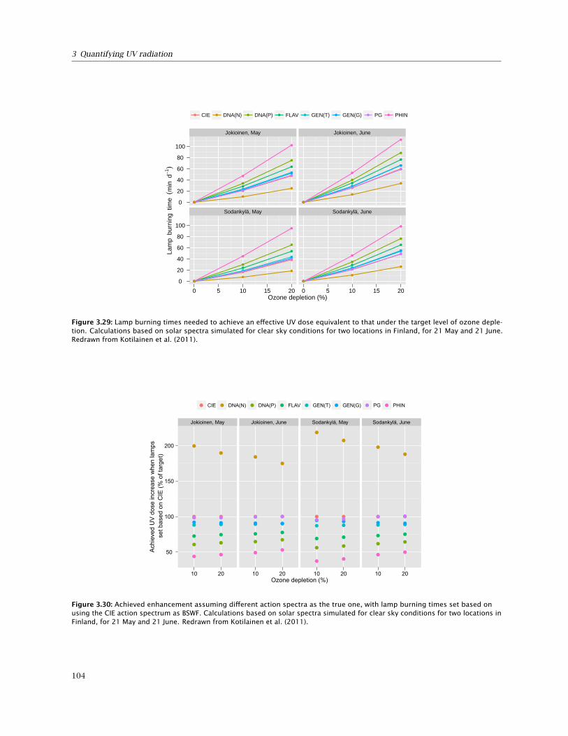
3 Quantifying UV radiation

Jokioinen, May Jokioinen, June

Sodankylä, May Sodankylä, June

0

20

40

60

80

100

0

20

40

60

80

100

0 5 10 15 20 0 5 10 15 20Ozone depletion (%)

Lam

p b

urni

ng t

ime

(min

d−1

)

CIE DNA(N) DNA(P) FLAV GEN(T) GEN(G) PG PHIN

Figure 3.29: Lamp burning times needed to achieve an effective UV dose equivalent to that under the target level of ozone deple-tion. Calculations based on solar spectra simulated for clear sky conditions for two locations in Finland, for 21 May and 21 June.Redrawn from Kotilainen et al. (2011).

Jokioinen, May Jokioinen, June Sodankylä, May Sodankylä, June

50

100

150

200

10 20 10 20 10 20 10 20Ozone depletion (%)

Ach

ieve

d U

V d

ose

incr

ease

whe

n la

mps

set

bas

ed o

n C

IE (%

of t

arge

t)

CIE DNA(N) DNA(P) FLAV GEN(T) GEN(G) PG PHIN

Figure 3.30: Achieved enhancement assuming different action spectra as the true one, with lamp burning times set based onusing the CIE action spectrum as BSWF. Calculations based on solar spectra simulated for clear sky conditions for two locations inFinland, for 21 May and 21 June. Redrawn from Kotilainen et al. (2011).

104

3.11 Effective UV doses outdoors

on the BSWF used as long as the shade is ‘gray’ (equallyaffects all relevant wavelengths). However, how much UVfrom the lamps will be needed to compensate for thiswill depend on the BSWF used (Table 3.5). With someBSWFs the lamp power or burning time needed to com-pensate for shading is much more than that needed tosimulate ozone depletion, because with spectra like PG,we need to replace shaded UV-A with UV-B from lamps.See section 3.10 on page 101 for a discussion of the rela-tionship between changes in ozone column and changesin effective UV radiation.

To minimize shading errors we must build lamp framesthat produce little shade. Probably <5% shading is achiev-able. We should not attempt to compensate for shadingby the frames with UV from lamps. Shifting the wholeexperiment’s UV baseline dose by a small percentage butkeeping the size of enhancement at the target level isprobably the best approach available.

3.11 Effective UV doses outdoors: seasonaland latitudinal variation

The state of the atmosphere (in terms of ozone columnthickness, cloudiness and aerosol content) together withday-length and daily course of the solar zenith angle (θ)are the main factors determining the climatology of UV(and its components, UV-B and UV-A) at ground level. Forclear sky conditions the average spatial and temporal dis-tribution of UV irradiance can be computed by means ofa radiative transfer model fed with proper O3 and aerosoldata (Grifoni et al., 2009, 2008). In these conditions thelatitudinal and temporal distribution of UV irradiance aredriven mainly by two factors: day-length and θ throughthe day. See section 3.9 on page 97 for a discussion ofdifferent approaches to modelling.

To go from the climatology of UV spectral irradiance tothat of the biologically effective UV (UVBE) exposures (ordoses), spectral irradiance has to be weighted to accountfor the different efficiency of each wavelength in produ-cing biological effects; this is done applying a BSWF—based on the action spectrum of the biological processconsidered. Plant action spectra differ in the weight givento UV-B and UV-A radiation, as it has been illustrated insection 1.8 on page 21. In this analysis Grifoni et al.(2009) considered two action spectra related to plant re-sponse: the so-called Generalized Plant Action spectrum(GEN, proposed by Caldwell, 1971) and the more recentPlant Growth spectrum (PG, Flint and Caldwell, 2003).The erythemal action spectrum (CIE, McKinlay and Diffey,1987) was also included since instruments with a spec-tral sensibility quite close to it have been used in severalfield experiments. The analysis presented in this sectionwas based on spectral global irradiance for cloud-free

conditions on horizontal surfaces simulated by meansof the STAR model (Ruggaber et al., 1994; Schwanderet al., 2000) for Rome, Italy (lat. 41.88 N, long. 12.47E), Potsdam, Germany (lat. 52.40 N, long. 13.03 E) andTrondheim, Norway (lat. 63.42 N, long. 10.42 E) on thefirst day of each month of the year from 1:00 to 23:00(UTC time) with a 30 min time step. Daily UVBE doses(kJ m−2 d−1) were calculated for all these 12 days.

After convoluting the UV spectral energy irradiancesat ground level for the three locations and seasons withthe three BSWFs, a picture of the seasonal of UVBE radi-ation was obtained, which was different depending onlatitude. The pattern of seasonal and latitudinal variationof the daily UVBE doses is shown to depend strongly onthe BSWF, and day of the year (Table 3.6).

The changes in daily UVBE doses occurring through theyear relative to the yearly average, for the three locationsacross Europe illustrate the effect of action spectra usedas BSWFs (Figure 3.31).

The largest seasonal variation occurs when the UVBE

daily doses are computed on the basis of action spec-tra completely or partially excluding the contributionof the UV-A component, as in the case of GEN and CIErespectively. Figure 3.31 shows the extent to which latit-ude affects these seasonal changes, which have a largeramplitude as the latitude increases. In other words, theclimatology of UVBE appears to be strongly dependenton the action spectrum used, and, as different plant re-sponses follow different action spectra, the effective UVclimatology will depend on the plant response understudy.

These differences in climatology are ecologically relev-ant, for instance for perennial species that may exper-ience different seasonal change in the UVBE irradiancethey are exposed to, depending on the latitude at whichthey are growing and on the biological process/actionspectrum studied.

3.12 Effective UV doses in controlledenvironments

If the light spectrum in a controlled environment differsgreatly from that under natural conditions, the relat-ive biologically effective irradiances will differ greatlydepending on the action spectrum used as BSWF. For ex-ample, if UV-A irradiance is much lower in daylight thanin the controlled environment, but UV-B irradiance sim-ilar to that in daylight, the dose calculated using GEN(G)as a BSWF will differ little between the controlled en-vironment and daylight, but the dose based on PG willbe much lower in the controlled environment than indaylight. This example shows why we need to use a real-istic light spectrum in controlled environments when we

105

3 Quantifying UV radiation

Trondheim

Potsdam

Rome

0

1

2

3

0

1

2

3

0

1

2

3

1 Jan

1 Feb1 Mar

1 Apr1 May

1 Jun

1 Jul

1 Aug1 Sep

1 Oct1 Nov

1 Dec

Time of year

Effe

ctiv

e do

se re

lativ

e to

yea

rly m

ean

effe

ctiv

e do

se

CIE GEN(G) PG

Figure 3.31: Relative seasonal variation of daily biologically effective UV doses for Trondheim, Potsdam and Rome, calculatedusing three different BSWFs. Actual values are normalized by division by the yearly average for each location. The horizontaldotted line shows the normalized mean. See Table 1.4 on page 25 for references to the sources of the spectra used as BSWFs.

106

3.13 An accuracy ranking of quantification methods

Table 3.6: Seasonal and latitudinal variation in effective UV doses across Europe. Daily doses (kJ m−2 d−1) at three times of theyear at three locations. Modelled values for clear sky conditions. See text for details. See Table 1.4 on page 25 for references tothe sources of the spectra used as BSWFs.

Date City CIE GEN(G) PG

1 Jan Trondheim 0.028 0.008 0.651 Jan Potsdam 0.161 0.047 3.251 Jan Rome 0.515 0.296 7.77

1 Apr Trondheim 0.92 0.528 13.871 Apr Potsdam 1.56 1.27 18.781 Apr Rome 2.46 2.48 24.70

1 Jul Trondheim 3.41 3.67 32.301 Jul Potsdam 4.07 4.77 34.601 Jul Rome 4.90 6.23 37.08

want to extrapolate the results from such experimentsto natural conditions. Furthermore, an increased ratiobetween UV-B and UV-A radiation, and/or UV-B radiationand PAR artificially enhances the responses of plants toUV-B radiation.

3.13 An accuracy ranking of quantificationmethods

Table 3.7 shows a preliminary comparison of differentmethods available for quantifying solar UV radiation andestimating biologically effective doses. Bias is the system-atic directional deviation from the true value, for exampleoverestimation of irradiance or doses. Uncertainty is arandom deviation that prevents us from knowing the truevalue, but deviations are not systematic —measurementsfrom different instruments or the same instruments afterdifferent recalibrations will deviate by different amountsand in different directions from the true value.

A detailed comparison is difficult with the informationcurrently available, consequently some gaps remain inthe table. However, some general recommendations arepossible. For outdoors experiments with manipulationof solar UV, the best option is most probably a combin-ation of (a) hourly simulation of UV spectral irradiancewith a model using ground station data as input, plus (b)spot measurements, for example under different filterswith a spectroradiometer under clear sky conditions. Itis best to replace modelling (a) with actual continuousmeasurements with a well calibrated double monochro-mator spectroradiometer. However, this is rarely possiblein practice, as there are few ground stations producingvalidated spectral data.

For experiments using lamps, the best option from thepoint of view of accuracy is the use of a double mono-chromator spectroradiometer. From a practical view-

point, using a broadband instrument calibrated against adouble monochromator spectroradiometer, may be easier.When measuring mixed daylight and lamp radiation, ormixed radiation from diverse lamps, or when there isdegradation of filters, broadband instruments are totallyunsuitable.

Single monochromator spectroradiometers should beavoided for measurements of UV-B radiation when thereis a background of UV-A or visible radiation, unless veryspecial handling of stray light is done by a combinationof special measuring protocols and data processing.

3.14 Sanity checks for data and calculations

When quantifying UV radiation, or in fact when doingany measurement, one should compare the values (e.g.irradiances or daily doses) against what has earlier beenreported in the literature for a similar light source. Inthis way many errors can be detected. To help in thisprocess we present in Table 3.8 typical values for bothunweighted UV-A and UV-B (energy) irradiance, photonirradiance, and biologically effective irradiances with themost frequently used BSWFs and wavelength normalisa-tions. For UV radiation outdoors one can use a model(e.g. TUV quick simulator) to estimate spectral irradiancevalues and from them calculate effective doses or expos-ure. We have done these calculations for some sites, andpresent them in Table 3.8. We have also included datafor some lamps.

3.15 Recommendations

In this section we list recommendations related to thequantification of UV radiation in experiments. See sec-tions 2.6.1 and 2.6.2 for recommendations on manipu-lation of UV radiation, section 4.9 for recommendations

107

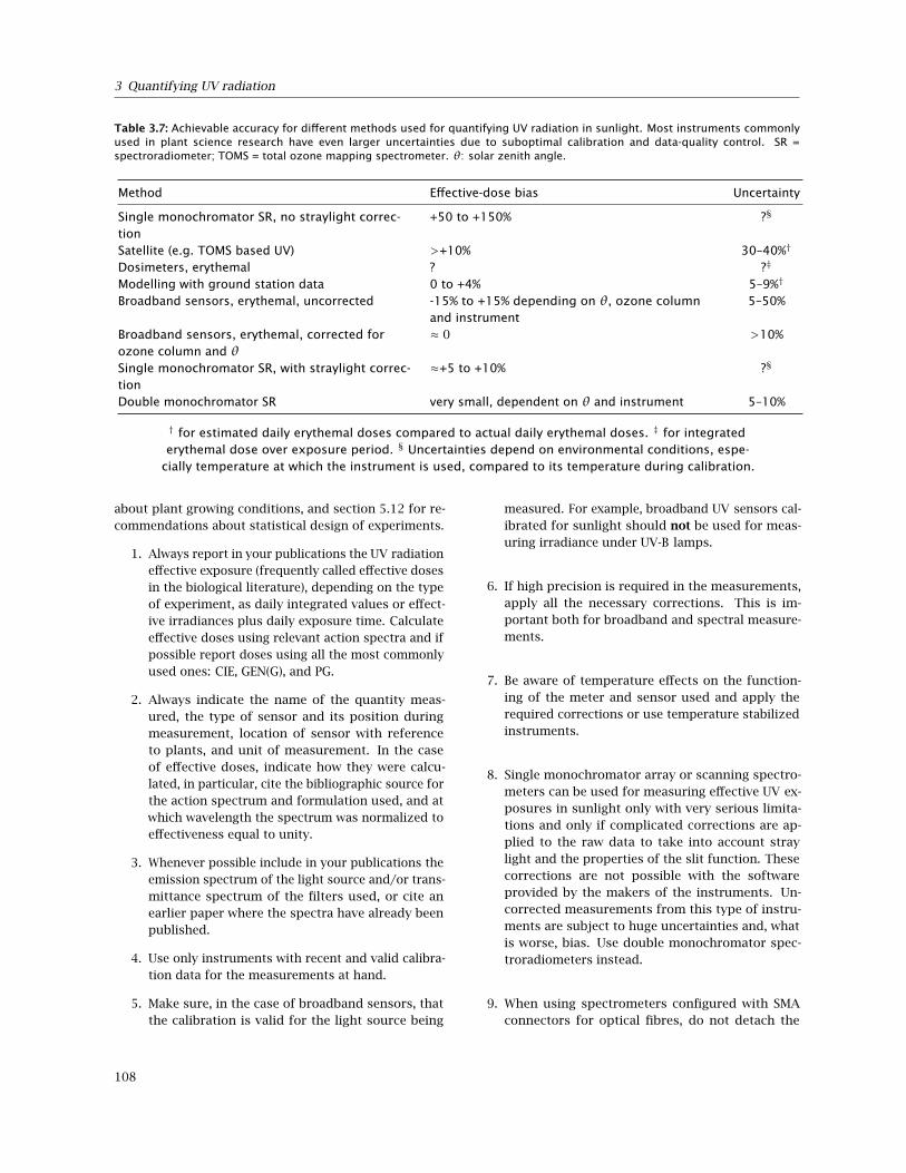
3 Quantifying UV radiation

Table 3.7: Achievable accuracy for different methods used for quantifying UV radiation in sunlight. Most instruments commonlyused in plant science research have even larger uncertainties due to suboptimal calibration and data-quality control. SR =spectroradiometer; TOMS = total ozone mapping spectrometer. θ: solar zenith angle.

Method Effective-dose bias Uncertainty

Single monochromator SR, no straylight correc-tion

+50 to +150% ?§

Satellite (e.g. TOMS based UV) >+10% 30–40%†

Dosimeters, erythemal ? ?‡

Modelling with ground station data 0 to +4% 5–9%†

Broadband sensors, erythemal, uncorrected -15% to +15% depending on θ, ozone columnand instrument

5–50%

Broadband sensors, erythemal, corrected forozone column and θ

≈ 0 >10%

Single monochromator SR, with straylight correc-tion

≈+5 to +10% ?§

Double monochromator SR very small, dependent on θ and instrument 5–10%

† for estimated daily erythemal doses compared to actual daily erythemal doses. ‡ for integratederythemal dose over exposure period. § Uncertainties depend on environmental conditions, espe-

cially temperature at which the instrument is used, compared to its temperature during calibration.

about plant growing conditions, and section 5.12 for re-commendations about statistical design of experiments.

1. Always report in your publications the UV radiationeffective exposure (frequently called effective dosesin the biological literature), depending on the typeof experiment, as daily integrated values or effect-ive irradiances plus daily exposure time. Calculateeffective doses using relevant action spectra and ifpossible report doses using all the most commonlyused ones: CIE, GEN(G), and PG.

2. Always indicate the name of the quantity meas-ured, the type of sensor and its position duringmeasurement, location of sensor with referenceto plants, and unit of measurement. In the caseof effective doses, indicate how they were calcu-lated, in particular, cite the bibliographic source forthe action spectrum and formulation used, and atwhich wavelength the spectrum was normalized toeffectiveness equal to unity.

3. Whenever possible include in your publications theemission spectrum of the light source and/or trans-mittance spectrum of the filters used, or cite anearlier paper where the spectra have already beenpublished.

4. Use only instruments with recent and valid calibra-tion data for the measurements at hand.

5. Make sure, in the case of broadband sensors, thatthe calibration is valid for the light source being

measured. For example, broadband UV sensors cal-ibrated for sunlight should not be used for meas-uring irradiance under UV-B lamps.

6. If high precision is required in the measurements,apply all the necessary corrections. This is im-portant both for broadband and spectral measure-ments.

7. Be aware of temperature effects on the function-ing of the meter and sensor used and apply therequired corrections or use temperature stabilizedinstruments.

8. Single monochromator array or scanning spectro-meters can be used for measuring effective UV ex-posures in sunlight only with very serious limita-tions and only if complicated corrections are ap-plied to the raw data to take into account straylight and the properties of the slit function. Thesecorrections are not possible with the softwareprovided by the makers of the instruments. Un-corrected measurements from this type of instru-ments are subject to huge uncertainties and, whatis worse, bias. Use double monochromator spec-troradiometers instead.

9. When using spectrometers configured with SMAconnectors for optical fibres, do not detach the

108

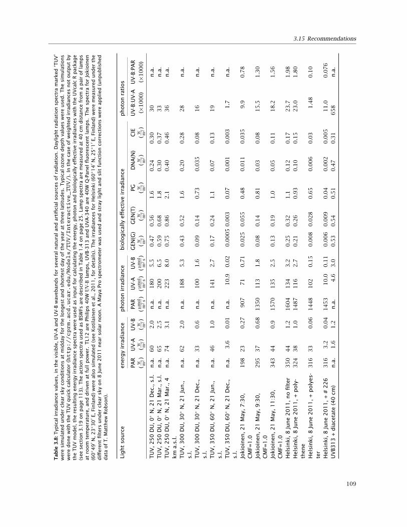
3.15 Recommendations

Tab

le3

.8:T

ypic

alir

radia

nce

valu

es,

inth

evi

sible

,U

V-A

and

UV

-Bw

aveb

ands

for

seve

ralnat

ura

lan

dar

tifi

cial

sourc

esof

radia

tion.

Day

light

radia

tion

spec

tra

mar

ked

‘TU

V’

wer

esi

mula

ted

under

clea

rsk

yco

ndit

ions

atm

idday

for

the

longes

tan

dsh

ort

est

day

of

the

year

atth

ree

lati

tudes

.Typ

ical

ozo

ne

dep

thva

lues

wer

euse

d.

The

sim

ula

tions

wer

edone

wit

hth

eT

UV

quic

kca

lcula

tor

(http://cprm.acd.ucar.edu/Models/TUV/Interactive_TUV/

).In

the

case

of

wei

ghte

dir

radia

nce

snot

outp

ut

by

the

TU

Vm

odel

,th

ere

sult

ing

ener

gy

irra

dia

nce

spec

tra

wer

euse

das

input

for

calc

ula

ting

the

ener

gy,

photo

nan

dbio

logic

ally

effec

tive

irra

dia

nce

sw

ith

the

UV

calc

Rpac

kag

e(s

eese

ctio

n3

.19

on

pag

e1

13

).The

acti

on

spec

tra

use

das

BSW

Fsar

edes

crib

edin

Tab

le1

.4on

pag

e25

.La

mp

spec

tra

are

mea

sure

dat

40

cmdis

tance

from

apai

rof

lam

ps

atro

om

tem

per

ature

,an

ddri

ven

atfu

llpow

er.

TL1

2ar

ePh

ilip

s4

0W

UV

-Bla

mps,

UV

B-3

13

and

UV

A-3

40

are

40

WQ

-Pan

elfl

uore

scen

tla

mps.

The

spec

tra

for

Jokio

inen

(60 4

9′ N

,23 3

0′ E

,Fi

nla

nd)

wer

eal

sosi

mula

ted

(see

Koti

lain

enet

al.,

20

11

,fo

rdet

ails

).The

irra

dia

nce

sfo

rH

elsi

nki(6

0 1

4′ N

,25 1′ E

,Fi

nla

nd)

wer

em

easu

red

under

the

diff

eren

tfi

lter

sunder

clea

rsk

yon

8Ju

ne

20

11

nea

rso

lar

noon.

AM

aya

Pro

spec

trom

eter

was

use

dan

dst

ray

light

and

slit

funct

ion

corr

ecti

ons

wer

eap

plied

(unpublish

eddat

aof

T.

Mat

thew

Robso

n).

Light

sourc

een

ergy

irra

dia

nce

photo

nir

radia

nce

bio

logic

ally

effec

tive

irra

dia

nce

photo

nra

tios

PAR

UV

-AU

V-B

PAR

UV

-AU

V-B

GEN

(G)

GEN

(T)

PGD

NA

(N)

CIE

UV

-B:U

V-A

UV

-B:P

AR

(W m

2)

(W m

2)

(W m

2)

(µm

ol

m2

s)

(µm

ol

m2

s)

(µm

ol

m2

s)

(W m

2)

(W m

2)

(W m

2)

(W m

2)

(W m

2)

(×1000)

(×1000)

TU

V,

25

0D

U,

0

N,

21

Dec

.,s.

l.n.a

.60

2.0

n.a

.180

5.5

0.4

70.5

61.6

0.2

40.3

030

n.a

.T

UV

,2

50

DU

,0

N,

21

Mar

.,s.

l.n.a

.65

2.5

n.a

.200

6.5

0.5

90.6

81.8

0.3

00.3

733

n.a

.TU

V,25

0D

U,0

N,21

Mar

.,4

km

a.s.

l.n.a

.74

3.1

n.a

.223

8.0

0.7

50.8

62.1

0.4

00.4

636

n.a

.

TU

V,3

00

DU

,3

0

N,21

Jun.,

s.l.

n.a

.62

2.0

n.a

.188

5.3

0.4

30.5

21.6

0.2

00.2

828

n.a

.

TU

V,3

00

DU

,3

0

N,21

Dec

.,s.

l.n.a

.33

0.6

n.a

.100

1.6

0.0

90.1

40.7

30.0

35

0.0

816

n.a

.

TU

V,3

50

DU

,6

0

N,21

Jun.,

s.l.

n.a

.46

1.0

n.a

.141

2.7

0.1

70.2

41.1

0.0

70.1

319

n.a

.

TU

V,3

50

DU

,6

0

N,21

Dec

.,s.

l.n.a

.3.6

0.0

1n.a

.10.9

0.0

20.0

005

0.0

03

0.0

70.0

01

0.0

03

1.7

n.a

.

Jokio

inen

,21

May

,7

:30

,C

MF=

1.0

198

23

0.2

7907

71

0.7

10.0

25

0.0

55

0.4

80.0

11

0.0

35

9.9

0.7

8

Jokio

inen

,21

May

,9

:30

,C

MF=

1.0

295

37

0.6

81350

113

1.8

0.0

80.1

40.8

10.0

30.0

815.5

1.3

0

Jokio

inen

,21

May

,1

1:3

0,

CM

F=1

.0343

44

0.9

1570

135

2.5

0.1

30.1

91.0

0.0

50.1

118.2

1.5

6

Hel

sinki,

8Ju

ne

20

11

,no

filt

er350

44

1.2

1604

134

3.2

0.2

50.3

21.1

0.1

20.1

723.7

1.9

8H

elsi

nki,

8Ju

ne

20

11

,+

poly

-th

ene

324

38

1.0

1487

116

2.7

0.2

10.2

60.9

30.1

00.1

523.0

1.8

0

Hel

sinki,

8Ju

ne

20

11

,+

poly

es-

ter

316

33

0.0

61448

102

0.1

50.0

08

0.0

28

0.6

50.0

06

0.0

31.4

80.1

0

Hel

sinki,

8Ju

ne

20

11

,+

#2

26

316

3.2

0.0

41453

10.0

0.1

10.0

06

0.0

09

0.0

40.0

02

0.0

05

11.0

0.0

76

UV

B3

13

+dia

ceta

te(4

0cm

)n.a

.1.6

1.2

n.a

.4.6

3.0

0.5

30.5

40.5

10.4

70.3

1658

n.a

.

109

3 Quantifying UV radiation

fibre at the spectrometer end1011. Doing so inval-idates the calibration because the alignment of thefibre with respect to the entrance slit may be differ-ent after the fibre is reattached.

10. When measuring, take into account the field ofview of the entrance optics of your instrument (e.g.one hemisphere for a cosine corrected irradiancesensor) and make sure that yourself and any othernearby objects do not disturb the radiation ‘seen’by the instrument.

11. Take into account that spot measurements of UVin sunlight under different filters describe only onepoint in time. Continuous measurements or model-ling based on continuous ground-based measure-ments are needed to fully describe the treatmentsapplied.

12. Outdoor UV irradiance is affected by cloudiness, someasurements where a single instrument is movedto take sequential measurements under the differ-ent treatments should be avoided unless the sky isperfectly clear. In addition, parallel measurementof PAR or global radiation in the open is recommen-ded so as to be able to detect any variation due toclouds.

13. UV exposure values (also called doses) derivedfrom satellite-based measurements are subject torelatively large errors and bias, so it is better toavoid their use, specially when daily or weekly val-ues are needed. Much of the uncertainty derivesfrom the sparse nature of the satellite data (e.g. oneor fewer fly overs per day).

14. Routinely check your instruments. Frequentlycheck that the readings are very close to zero whenthe sensor is in darkness. Do sanity checks on yourdata against values expected (e.g. using models orpublished data). For example if when measuring asunlight spectrum you get spectral irradiance val-ues different from zero12 at wavelengths shorterthan 290 nm you can be sure that there is a prob-lem. There may be too much stray light, or a badcorrection for the dark signal, or simply the spec-trometer is not good enough for the job.

15. When measuring sunlight or lamp spectra for cal-culating effective UV doses you need a spectrora-diometer with a spectral resolution of at least 1 nm.

Furthermore to reduce noise use only averagingof repeated scans rather than ‘Boxcar smoothing’.Boxcar smoothing reduces the spectral resolutionby doing a moving average across wavelengths.

3.16 Further reading

3.16.1 UV climatology and modelling

http://cprm.acd.ucar.edu/Models/TUV/Interactive_TUV/http://zardoz.nilu.no/~olaeng/fastrt/http://jwocky.gsfc.nasa.gov/teacher/ozone_overhead.html

3.16.2 Instrumentation and UV measurementvalidation

The report A Guide to Spectroradiometry: Instruments& Applications for the Ultraviolet (Bentham, 1997) de-scribes scanning spectroradiometers. It is available athttp://www.bentham.co.uk/pdf/UVGuide.pdf. The report Instruments to Measure Solar Ultra-violet Radiation - Part 4: Array Spectroradiometers(Seckmeyer, Bais, Bernhard, Blumthaler, Drüke et al.,2010) gives guidelines for the use of array spectro-meters for measuring UV-B radiation. This report isavailable at http://www.wmo.int/pages/prog/arep/gaw/documents/GAW191_TD_No_1538_web.pdf. The report Instruments to Measure SolarUltraviolet Radiation - Part 3: Multi-channel filter instru-ments (Seckmeyer, Bais, Bernhard, Blumthaler, Johnsenet al., 2010) is available at http://www.wmo.int/pages/prog/arep/gaw/documents/GAW190_TD_No_1537_web.pdf. The report Instruments toMeasure Solar Ultraviolet Radiation Part 2: BroadbandInstruments Measuring Erythemally Weighted Solar Irra-diance (Seckmeyer et al., 2005) is available at ftp://ftp.wmo.int/Documents/PublicWeb/arep/gaw/final_gaw164_bookmarks_17jul.pdf,while the first report of the series, titled Instrumentsto Measure Solar Ultraviolet Radiation - Part 1: SpectralInstruments (Seckmeyer et al., 2001) is only available inprinted form.

10SMA connectors were originally designed for attaching light fibres used in digital communications, and do not guarantee repeatability of thefibre’s alignment. Other types of connectors (e.g. FC) that provide better repeatability are available as an additional cost option from somespectrometer manufacturers.

11Detaching the fibre from the diffuser does not invalidate the calibration as small changes in alignment will not change the amount of radiationentering the fibre.

12You may be thinking how close to zero is close enough. For reliably measuring effective UV doses in sunlight using a spectroradiometer oneneeds at least four or five orders of magnitude between the highest peak in the visible and the noise signal.

110

3.17 Appendix: Formulations for action spectra used as BSWFs

3.16.3 Books

The book Radiation Measurement in Photobiology editedby Diffey (1989) includes information on detectors and

methods not described in this handbook, or that aredescribed here in less detail.

3.17 Appendix: Formulations for action spectra used as BSWFs

The calculation of biologically effective UV doses requires weighting the spectral energy irradiance (E) or spectralphoton irradiance (Q) at each wavelength with a weighting value that is typically generated from a mathematicalformulation fitted to describe the weighting function or action spectrum of the biological process—i.e. a biologicalspectral weighting function (BSWF). Data obtained from a spectroradiometer are usually provided as spectral energyirradiance (units: W m−2 nm−1) and care should be taken to use the appropriate formulation that uses either energyeffectiveness (s) or quantum effectiveness (sp) values as appropriate.

The usual approach is to base effective UV doses on energy irradiance data, using BSWFs that provide values forrelative energy effectiveness at each wavelength. However, BSWFs are often defined using quantum effectivenessfor application to photon irradiance values. Consequently, conversion of energy irradiance values measured duringexperiments to photon irradiance is necessary before applying weighting functions originally formulated usingquantum effectiveness. Conversion of energy irradiance values to photon irradiance can be achieved using equation 3.1on page 72. After conversion, the calculated effective doses will be on a different scale than if they are calculated basedon energy irradiance values. Note that you may find examples in the literature where formulations based on quantumeffectiveness (sp) have been inappropriately applied to spectral energy exposure (unit: J m−2 nm−1) or spectral energyirradiance (unit: W m−2 nm−1).

The general plant action spectrum of Caldwell (Code GEN in Table 1.4 on page 25) was originally published simplyas a graphical figure of quantum effectiveness against wavelength (Caldwell, 1971) and subsequently two publicationshave fitted different mathematical formulations to describe its use as a weighting function. Green et al. (1974) fitted afunction that decreases to zero at 313 nm whereas an alternative mathematical fit provided by Thimijan et al. (1978)continues to weight irradiance values up to 345 nm in the UV-A region. Both of these functions are shown on Figure1.19 on page 25 as GEN(G) and GEN(T) respectively. It is important to specify which mathematical function has beenused when describing the calculation of effective UV doses in experimental methods.

The general plant action spectrum of Caldwell fitted with the mathematical function of Green et al. (1974) is givenby (Source: Björn and Teramura, 1993):

spGEN(G)(λ) =

2.618 ·[

1−(

λ313.3

)2]· e−

λ−30031.08 if λ ≤ 313.3 nm

0 if λ > 313.3 nm(3.7)

and when fitted with the mathematical function of Thimijan et al. (1978) is given by (Source: Björn and Teramura,1993):

spGEN(T)(λ) =

e−

(265−λ

21

)2

if λ ≤ 345 nm0 if λ > 345 nm

(3.8)

The DNA damage formulation of Green and Miller (1975) is given by:

spDNA(GM)(λ) = e

13.82·(1+e

λ−3109

)−1

−1

(3.9)

The doses calculated with this formulation differ significantly from doses calculated using tabulated values derivedfrom the figure in Setlow (1974). For example the model TUV and the data from the NSF UV monitoring network usethe tabulated values rather than the formulation by Green and Miller (1975).

However, most BSWFs are conventionally used with a value of one at 300 nm. This may be achieved by simplecalculation adjustments within a spreadsheet (by dividing each wavelength effectiveness by the effectiveness value at300 nm) or by altering the mathematical formula directly. Thus, the mathematical formulation of Green et al. (1974)

111

3 Quantifying UV radiation

for GEN(G) requires equation 3.7 to be multiplied by 4.596 to normalize it to a value of 1 at 300nm and similarlyGEN(T) requires equation 3.8 to be multiplied by 16.083 and DNA(GM) requires equation 3.9 to be multiplied by 30.675.

The formulation of the weighting function published by Flint and Caldwell (2003) for plant growth, shown as PG inFigure 1.19 on page 25, was for quantum effectiveness and already provides normalization to 1 at 300 nm and is givenby:

spPG(λ) =

exp (4.688272 ·

exp(− exp

(0.1703411 · λ−307.867

1.15

))+(

390−λ121.7557 − 4.183832

))if λ ≤ 390 nm

0 if λ > 390 nm

(3.10)

Some weighting functions are already defined using energy effectiveness values for use with energy irradiance data,one example being the CIE erythemal action spectrum (McKinlay and Diffey, 1987; A. R. Webb et al., 2011). The standardwas revised in 1998 and the updated version should be used instead of the original one from 1987 (A. R. Webb et al.,2011). It is important to check that published mathematical formulae have been appropriately normalized to oneat 300 nm. However, whereas most BSWFs are conventionally set to one at 300 nm, the CIE98 erythemal weightingfunction has defined values at specific wavelengths (A. R. Webb et al., 2011) and is given by:

sCIE(λ) =

1 if 250 ≤ λ ≤ 298 nm100.094(298−λ) if 298 ≤ λ ≤ 328 nm100.015(140−λ) if 328 ≤ λ ≤ 400 nm0 if λ > 400

(3.11)

Weighting functions defined using quantum effectiveness (sp(λ)), and normalized to one at 300 nm, can be convertedto relative energy effectiveness (s(λ)) simply by multiplication, wavelength by wavelength, of the quantum effectivenessby by the respective wavelength in nm and dividing by 300 (the chosen normalization wavelength in nm). The value300 should be changed when using other wavelengths for normalization. This is based on equation 3.1 giving theenergy in one photon, but as Planck’s constant (h) and the speed of light in vacuum (c) are constant divisors, and weare expressing the effectiveness in relative units, they can be left out of the calculation.

It is always essential to specify clearly the normalization wavelength, the mathematical formulation and the BSWFused when describing the calculation of effective UV doses.

3.18 Appendix: Calculation of effectivedoses with Excel

Let us start with a text file generated by a spectrora-diometer and its connected computer. With the instru-ments that I have used this text file consists of onecolumn, containing either spectral (energy) irradianceor spectral photon irradiance (some instruments, espe-cially for underwater use, may have fluence rate insteadof irradiance). At the start, above the columns, is a head-ing containing supplementary information. Other instru-ments may have two columns, the first one containingwavelength values, the other one spectral irradiance val-ues.

For the Optronics instruments that I have used, thestart of a data file looks like the listing in Figure 3.32.The heading here contains “a”, which in this case is thename of the file, the kind of data that is recorded (in-cluding the unit), the date, the starting wavelength innm, the end wavelength (not shown here) in nm, and thestep interval in nm. This file can be loaded into an Ex-cel file going to Data>Get external data>Loadtext file. When you have done this, insert a new

column to the left of the one containing the measureddata. In this new column you should fill in the wavelengthvalues, which can be done in the following way withouttyping every value:

Type the first two values, i.e. in this case first “250” inthe cell left of the one containing the first radiation value1.439562E-010. Since the step interval is 1.00 nm, thenext value is 251. Type this in the cell to the left of thevalue 1.797497E-010. Select the two cells that you havejust filled in. Put the cursor at the lower left corner ofthe cell containing “251” and see it change appearance,push the (left) mouse button and drag down to the cellleft of the last radiation value. The column will then fillup with the appropriate wavelength values.

You have now filled columns A and B with the appro-priate values. Next you should generate a column withvalues of the weighting function. Suppose you wish touse the weighting function of Flint and Caldwell (2003).The formula given for this in the publication is Biologic-ally effective UV= exp[4.688272∗exp(− exp(0.1703411∗(x−307.867)/1.15))+((390−x)/121.7557−4.183832)]in which x stands for wavelength in nm.

Select cells in column C over the rows corresponding to

112

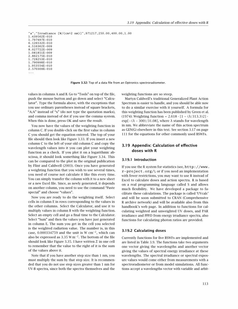
3.19 Appendix: Calculation of effective doses with R

"a","Irradiance [W/(cm^2 nm)]",971217,250.00,400.00,1.001.439562E-0101.797497E-0106.126532E-0104.516362E-0098.027722E-0091.081851E-0092.862175E-0101.728253E-0101.790998E-0101.953554E-0102.570309E-010...

Figure 3.32: Top of a data file from an Optronics spectroradiometer.

values in columns A and B. Go to “Tools” on top of the file,push the mouse button and go down and select “Calcu-lator”. Type the formula above, with the exceptions thatyou use ordinary parentheses instead of square brackets,“A:A” instead of “x” (do not type the quotation marks),and comma instead of dot if you use the comma system.When this is done, press OK and save the result.

You now have the values of the weighting function incolumn C. If you double-click on the first value in columnC you should get the equation entered. The top of yourfile should then look like Figure 3.33. If you insert a newcolumn C to the left of your old column C and copy thewavelength values into it you can plot your weightingfunction as a check. If you plot it on a logarithmic ab-scissa, it should look something like Figure 3.34. Thiscan be compared to the plot in the original publicationby Flint and Caldwell (2003). Once you have generateda weighting function that you wish to use several times,you need of course not calculate it like this every time.You can simply transfer the column with it to a new sheetor a new Excel file. Since, as newly generated, it dependson another column, you need to use the command “Pastespecial” and choose “values”.

Now you are ready to do the weighting itself. Selectcells in column E in rows corresponding to the values inthe other columns. Select the Calculator, and use it tomultiply values in column B with the weighting function.Select an empty cell and go a final time to the Calculator.Select “Sum” and then the values you have just generatedin column E. The sum you get in the cell you selectedis the weighted radiation value. The number is, in thiscase, 0.000334759 and the unit is W cm−2, which canalso be expressed as 3.35 W m−2. The bottom of the fileshould look like Figure 3.35. I have written Σ in one cellto remember that the value to the right of it is the sumof the values above it.

Note that if you have another step size than 1 nm, youmust multiply the sum by that step size. It is recommen-ded that you do not use step sizes greater than 1 nm forUV-B spectra, since both the spectra themselves and the

weighting functions are so steep.Martyn Caldwell’s traditional Generalized Plant Action

Spectrum is easier to handle, and you should be able nowto do a similar exercise with it yourself. A formula forthis weighting function has been published by Green et al.(1974): Weighting function = 2.618 · [1− (λ/313.3)2] ·exp[−(λ− 300)/31.08], where λ stands for wavelengthin nm. We abbreviate the name of this action spectrumas GEN(G) elsewhere in this text. See section 3.17 on page111 for the equations for other commonly used BSWFs.

3.19 Appendix: Calculation of effectivedoses with R

3.19.1 Introduction

If you use the R system for statistics (see, http://www.r-project.org/), or if you need an implementationwith fewer restrictions, you may want to use R instead ofExcel to calculate doses and action spectra. R is basedon a real programming language called S and allowsmuch flexibility. We have developed a package to fa-cilitate these calculations. The package is called ‘UVcalc’and will be soon submitted to CRAN (ComprehensiveR archive network) and will be available also from thishandbook’s web page. In addition to functions for cal-culating weighted and unweighted UV doses, and PARirradiance and PPFD from energy irradiance spectra, alsofunctions for calculating photon ratios are provided.

3.19.2 Calculating doses

Currently functions for five BSWFs are implemented andare listed in Table 3.9. The functions take two argumentsone vector giving the wavelengths and another vectorgiving the values of spectral energy irradiance at thesewavelengths. The spectral irradiance or spectral expos-ure values would come either from measurements with aspectroradiometer or from model simulations. All func-tions accept a wavelengths vector with variable and arbit-

113

3 Quantifying UV radiation

Figure 3.33: Screen capture from a Excel worksheet onto which spectral data have been imported.

Figure 3.34: Screen capture from a Excel plot of the plant growth action spectrum (PG).

Figure 3.35: Screen capture from the bottom of an Excel worksheet on which doses have been calculated.

114

3.19 Appendix: Calculation of effective doses with R

rary step sizes, with the condition that the wavelengthsare sorted in strictly increasing order, something which isespecially convenient when dealing with data from arrayspectrometers13.

The functions are made available by installing the pack-age UVcalc (once) and loading it from the library whenneeded. To load the package into the workspace uselibrary(UVcalc). Then load your spectral data intoR using read.table() or read.csv().

A file from a Macam spectroradiometer starts:

Wavelength (nm) ,W/m2270,0271,0272,1.17E−04273,2.42E−04274,4.55E−04275,8.94E−04276,0.00161277,0.00263278,0.00412279,0.00621280,0.00904281,0.01697282,0.02069283,0.02663284,0.03314285,0.04075286,0.04895287,0.05817288,0.0679

For a file like this one, use the code below but repla-cing "name" with the name and path to the data file. OnWindows systems you need to scape backslashes in filepaths like this: ‘\\’.my.data <- \read.csv(filename="name", skip=1,col.names=c("wavelength", "irrad"))

attach(my.data)GEN.G.dose(wavelength,irrad)PG.dose(wavelength,irrad)detach(my.data)

If our spectral irradiance data is in W m−2 nm−1, andthe wavelength in nm, as in the case of the Macam spec-troradiometer, the functions will return the effective irra-diance in W m−2.

If, for example, the spectral irradiance output by ourmodel or spectroradiometer is in mW m−2 nm−1, and thewavelengths are in Ångstrom then to obtain the effectiveirradiance in W m−2 we will need to convert the units....GEN.G.dose(wavelength/10, irrad/1000)PG.dose(wavelength/10, irrad/1000)...

In this example, we take advantage of the behaviourof the S language: an operation between a scalar and

vector, is equivalent to applying this operation to eachmember of the vector. Consequently, in the code above,each value from the vector of wavelengths is divided by10, and each value in the vector of spectral irradiances isdivided by 1000.

If the spectral irradiance is in mW cm−2 nm−1 thenvalues should be multiplied by 10 to convert them toW m−2 nm−1.

It is very important to make sure that the wavelengthsare in nanometers as this is what the functions expect. Ifthe wavelengths are in the wrong units, the BSWF will bewrongly calculated, and the returned value for effectiveirradiance will be wrong.

If we use as input to the functions instead of spec-tral irradiances, time-integrated spectral irradiances inkJ m−2 d−1 nm−1, then the functions will return the ef-fective exposure, or ‘dose’ in kJ m−2 d−1. Such time-integrated values are more frequently available as theoutput of models, or by integrating observed sequentialvalues of spectral irradiance.

In addition to the functions for calculating biolo-gically effective doses and effective irradiances, weprovide functions for calculating unweighted dosesor irradiances of PAR (PPFD() or PAR.q.dose(),and PAR.e.dose()), UV-A (UVA.q.dose() andUVA.e.dose()) and UV-B (UVB.q.dose() andUVB.e.dose()), where ‘e’ variants return energydoses, and ‘q’ variants return quantum or photon doses.All functions expect as input radiation spectra in energyunits, and wavelengths in nm.

3.19.3 Calculating an action spectrum at givenwavelengths

The functions available for calculating action spectra takeas argument a vector of wavelengths, and return a vec-tor of effectiveness (either quantum=photon or energybased) normalized to unity effectiveness at a wavelengthof 300 nm except when indicated. These functions arelisted in Table 3.10, and an example of their use follows.In these examples we generate the wavelengths vectorsin R, but they can be also read from a file.# at 1 nm intervalswavelengths1 <- 285:400action.spectrum1 <- GEN.T.e(wavelengths1)# at 0.1 nm intervalswavelengths01 <- seq(from = 285, to = 400, by = 0.1)action.spectrum01 <- GEN.T.e(wavelengths01)

All functions accept a wavelengths vector with vari-able and arbitrary step sizes, with the condition that thewavelengths are sorted in strictly increasing order.

13It is always best to use in calculations the data at the original wavelength of each pixel of the array of the spectrometer, rather than to produce aspectrum with ‘nice’ wavelength steps by interpolation.

115

3 Quantifying UV radiation

Table 3.9: Functions in R package UV.calc for calculation of unweighted and effective irradiances or doses, depending on whetherthey are used with an irradiance spectrum, or with daily total spectral exposure. The functions for effective (or weighted) irradiancesavailable in this package use different action spectra as BSWF, normalized to unity at different wavelengths (λ). w = vector ofwavelengths (nm); i = vector of spectral energy irradiances.

Action spectrum Formulation Dose or irrad. Norm. λ (nm)

Gen. plant action Green GEN.G.dose(w,i) 300Gen. plant action Thimijan GEN.T.dose(w,i) 300Plant growth Flint & Caldwell PG.dose(w,i) 300Erythemal CIE98 CIE.dose(w,i) 298‘Naked’ DNA TUV, from Setlow DNA.N.dose(w,i) 300‘Naked’ DNA Green & Miller DNA.GM.dose(w,i) 300‘Plant’ DNA Musil, from Quaite DNA.P.dose(w,i) 300UV-A (energy) n.a. UVA.e.dose(w,i) n.a.UV-A (photon) n.a. UVA.q.dose(w,i) n.a.UV-B (energy) n.a. UVB.e.dose(w,i) n.a.UV-B (photon) n.a. UVB.q.dose(w,i) n.a.PAR (energy) n.a. PAR.e.dose(w,i) n.a.PAR (photon) n.a. PAR.q.dose(w,i) n.a.

Table 3.10: Functions in R package UVcalc for calculation of action spectra. w = vector of wavelengths (nm).

Action spectrum Formulation Energy Quantum Norm. λ (nm)

Gen. plant action Green GEN.G.e(w) GEN.G.q(w) 300Gen. plant action Thimijan GEN.T.e(w) GEN.T.q(w) 300Plant growth Flint & Caldwell PG.e(w) PG.q(w) 300Erythemal CIE98 CIE.e(w) CIE.q(w) 298Erythemal CIE98 CIE.e300(w) CIE.q300(w) 300‘Naked’ DNA TUV, from Setlow DNA.N.e(w) DNA.N.q(w) 300‘Naked’ DNA Green & Miller DNA.GM.e(w) DNA.GM.q(w) 300‘Plant’ DNA Musil, from Quaite DNA.P.e(w) DNA.P.q(w) 300‘Plant’ DNA Musil, from Quaite DNA.P.e290(w) DNA.P.q290(w) 290

3.19.4 Calculating photon ratios

Functions are also provided for calculating photon ratiosbetween different pairs of wavebands. These functionsare listed in Table 3.11. We follow the most frequentlyused wavelength ranges for the different colours, butalso provide some generic functions that can be usedwhen other limits are needed. Continuing with the ex-ample above in which my.data was read and attached wecalculate UV-B : PAR photon ratio

UVB.PAR.ratio(wavelengths, irrad)

The spectral energy irradiance, can be in any energybased unit such as W m−2 nm−1, or mW cm−2 nm−1, as themultipliers cancel out when calculating the ratio. How-ever, wavelengths must be always expressed in nanomet-ers. Please, be aware that these functions will returnerroneous values if used with spectra expressed as spec-tral photon irradiance, even though the returned valuesare photon ratios.

Please, be aware that following common practice inthe literature, the wavelength range used for red light isdifferent for the different photon ratios.

3.19.5 Documentation

The package includes manual pages for the different func-tions, and an overview and a list of references for theoriginal sources used. The definition of the functionscan bee seen once the package is loaded by entering thename of the function without parameters or parentheses.

There are many resources on the R-System for Statisticsand statistics in general available on-line. The most use-ful ones are The R Wiki (http://rwiki.sciviews.org/), and the documentation included in all R installa-tions and accompanying each one of the different pack-ages.

Some classical books on R are those by Dalgaard (2002),Crawley (2005, 2007), and Venables and Ripley (2002).The book by Venables and Ripley, 2000 discusses pro-gramming in S, the language used in R to build newfunctions and packages.

3.20 Appendix: Suppliers of instruments

In this section we provide names and web addressesto some suppliers of instruments. This is certainly anincomplete list and exclusion reflects only our ignorance.

116

3.20 Appendix: Suppliers of instruments

Table 3.11: Functions in R package UVcalc for calculation of photon ratios from spectra in spectral energy units. w = vector ofwavelengths (nm); i = vector of spectral energy irradiances.

Ratio R function wavelength ranges (nm)

UV-B:UV-A UVB.UVA.ratio(w,i) 280–315, 315–400UV-B:PAR UVB.PAR.ratio(w,i) 280–315, 400–700UV-A:PAR UVA.PAR.ratio(w,i) 315–400, 400–700Red:Far-red R.FR.ratio(w,i) 650–670, 720–740Blue:Green B.G.ratio(w,i) 420–490, 500–570Blue:Red B.R.ratio(w,i) 420–490, 620–680

UV measurement:http://www.astranetsystems.com/http://www.avantes.com/http://www.bentham.co.uk/http://www.biosense.de/ (‘Viospore’ dosimet-ers.)http://www.biospherical.com/http://www.deltaohm.com/http://www.delta-t.co.uk/http://www.gigahertz-optik.de/http://www.goochandhousego.com/ (‘Optron-ics’ spectroradiometers)http://www.ictinternational.com.au/(ELDONET terrestrial dosimeters)http://www.intl-lighttech.com/http://www.irradian.co.uk/ (‘Macam’ instru-

ments under new name)http://www.kippzonen.com/http://www.oceanoptics.eu/http://www.roithner-laser.com/ (Photodi-odes)http://www.scitec.uk.com/http://www.sglux.com/ (SiC photodiodes, andinstruments)http://www.skyeinstruments.com/http://www.solarlight.com/http://www.spectralproducts.com/http://www.stellarnet.us/http://trios.de/ (RAMSES radiometers)http://www.yesinc.com/ (Yankee EnvironmentalSystems)

117

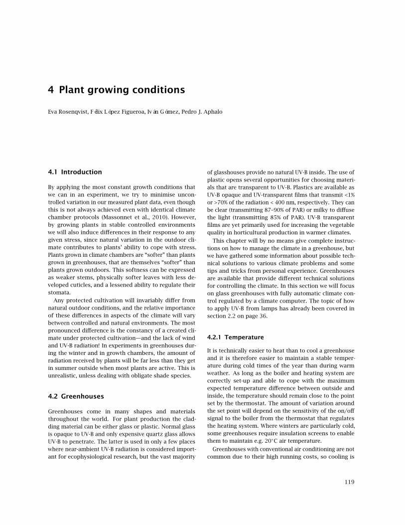
4 Plant growing conditions

Eva Rosenqvist, Félix López Figueroa, Iván Gómez, Pedro J. Aphalo

4.1 Introduction

By applying the most constant growth conditions thatwe can in an experiment, we try to minimise uncon-trolled variation in our measured plant data, even thoughthis is not always achieved even with identical climatechamber protocols (Massonnet et al., 2010). However,by growing plants in stable controlled environmentswe will also induce differences in their response to anygiven stress, since natural variation in the outdoor cli-mate contributes to plants’ ability to cope with stress.Plants grown in climate chambers are “softer” than plantsgrown in greenhouses, that are themselves “softer” thanplants grown outdoors. This softness can be expressedas weaker stems, physically softer leaves with less de-veloped cuticles, and a lessened ability to regulate theirstomata.

Any protected cultivation will invariably differ fromnatural outdoor conditions, and the relative importanceof these differences in aspects of the climate will varybetween controlled and natural environments. The mostpronounced difference is the constancy of a created cli-mate under protected cultivation—and the lack of windand UV-B radiation! In experiments in greenhouses dur-ing the winter and in growth chambers, the amount ofradiation received by plants will be far less than they getin summer outside when most plants are active. This isunrealistic, unless dealing with obligate shade species.

4.2 Greenhouses

Greenhouses come in many shapes and materialsthroughout the world. For plant production the clad-ding material can be either glass or plastic. Normal glassis opaque to UV-B and only expensive quartz glass allowsUV-B to penetrate. The latter is used in only a few placeswhere near-ambient UV-B radiation is considered import-ant for ecophysiological research, but the vast majority

of glasshouses provide no natural UV-B inside. The use ofplastic opens several opportunities for choosing materi-als that are transparent to UV-B. Plastics are available asUV-B opaque and UV-transparent films that transmit <1%or >70% of the radiation < 400 nm, respectively. They canbe clear (transmitting 87–90% of PAR) or milky to diffusethe light (transmitting 85% of PAR). UV-B transparentfilms are yet primarily used for increasing the vegetablequality in horticultural production in warmer climates.

This chapter will by no means give complete instruc-tions on how to manage the climate in a greenhouse, butwe have gathered some information about possible tech-nical solutions to various climate problems and sometips and tricks from personal experience. Greenhousesare available that provide different technical solutionsfor controlling the climate. In this section we will focuson glass greenhouses with fully automatic climate con-trol regulated by a climate computer. The topic of howto apply UV-B from lamps has already been covered insection 2.2 on page 36.

4.2.1 Temperature

It is technically easier to heat than to cool a greenhouseand it is therefore easier to maintain a stable temper-ature during cold times of the year than during warmweather. As long as the boiler and heating system arecorrectly set-up and able to cope with the maximumexpected temperature difference between outside andinside, the temperature should remain close to the pointset by the thermostat. The amount of variation aroundthe set point will depend on the sensitivity of the on/offsignal to the boiler from the thermostat that regulatesthe heating system. Where winters are particularly cold,some greenhouses require insulation screens to enablethem to maintain e.g. 20C air temperature.

Greenhouses with conventional air conditioning are notcommon due to their high running costs, so cooling is

119

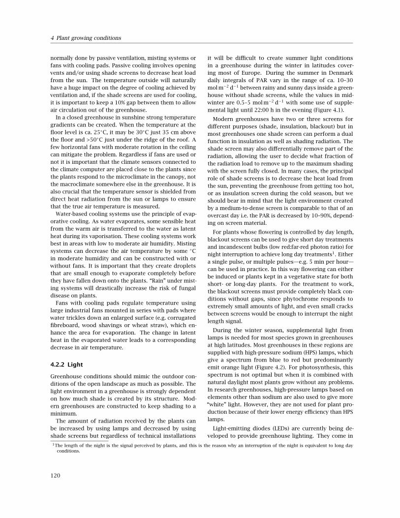
4 Plant growing conditions

normally done by passive ventilation, misting systems orfans with cooling pads. Passive cooling involves openingvents and/or using shade screens to decrease heat loadfrom the sun. The temperature outside will naturallyhave a huge impact on the degree of cooling achieved byventilation and, if the shade screens are used for cooling,it is important to keep a 10% gap between them to allowair circulation out of the greenhouse.

In a closed greenhouse in sunshine strong temperaturegradients can be created. When the temperature at thefloor level is ca. 25C, it may be 30C just 35 cm abovethe floor and >50C just under the ridge of the roof. Afew horizontal fans with moderate rotation in the ceilingcan mitigate the problem. Regardless if fans are used ornot it is important that the climate sensors connected tothe climate computer are placed close to the plants sincethe plants respond to the microclimate in the canopy, notthe macroclimate somewhere else in the greenhouse. It isalso crucial that the temperature sensor is shielded fromdirect heat radiation from the sun or lamps to ensurethat the true air temperature is measured.

Water-based cooling systems use the principle of evap-orative cooling. As water evaporates, some sensible heatfrom the warm air is transferred to the water as latentheat during its vaporisation. These cooling systems workbest in areas with low to moderate air humidity. Mistingsystems can decrease the air temperature by some Cin moderate humidity and can be constructed with orwithout fans. It is important that they create dropletsthat are small enough to evaporate completely beforethey have fallen down onto the plants. “Rain” under mist-ing systems will drastically increase the risk of fungaldisease on plants.

Fans with cooling pads regulate temperature usinglarge industrial fans mounted in series with pads wherewater trickles down an enlarged surface (e.g. corrugatedfibreboard, wood shavings or wheat straw), which en-hance the area for evaporation. The change in latentheat in the evaporated water leads to a correspondingdecrease in air temperature.

4.2.2 Light

Greenhouse conditions should mimic the outdoor con-ditions of the open landscape as much as possible. Thelight environment in a greenhouse is strongly dependenton how much shade is created by its structure. Mod-ern greenhouses are constructed to keep shading to aminimum.

The amount of radiation received by the plants canbe increased by using lamps and decreased by usingshade screens but regardless of technical installations

it will be difficult to create summer light conditionsin a greenhouse during the winter in latitudes cover-ing most of Europe. During the summer in Denmarkdaily integrals of PAR vary in the range of ca. 10–30mol m−2 d−1 between rainy and sunny days inside a green-house without shade screens, while the values in mid-winter are 0.5–5 mol m−2 d−1 with some use of supple-mental light until 22:00 h in the evening (Figure 4.1).

Modern greenhouses have two or three screens fordifferent purposes (shade, insulation, blackout) but inmost greenhouses one shade screen can perform a dualfunction in insulation as well as shading radiation. Theshade screen may also differentially remove part of theradiation, allowing the user to decide what fraction ofthe radiation load to remove up to the maximum shadingwith the screen fully closed. In many cases, the principalrole of shade screens is to decrease the heat load fromthe sun, preventing the greenhouse from getting too hot,or as insulation screen during the cold season, but weshould bear in mind that the light environment createdby a medium-to-dense screen is comparable to that of anovercast day i.e. the PAR is decreased by 10–90%, depend-ing on screen material.

For plants whose flowering is controlled by day length,blackout screens can be used to give short day treatmentsand incandescent bulbs (low red:far-red photon ratio) fornight interruption to achieve long day treatments1. Eithera single pulse, or multiple pulses—e.g. 5 min per hour—can be used in practice. In this way flowering can eitherbe induced or plants kept in a vegetative state for bothshort- or long-day plants. For the treatment to work,the blackout screens must provide completely black con-ditions without gaps, since phytochrome responds toextremely small amounts of light, and even small cracksbetween screens would be enough to interrupt the nightlength signal.

During the winter season, supplemental light fromlamps is needed for most species grown in greenhousesat high latitudes. Most greenhouses in these regions aresupplied with high-pressure sodium (HPS) lamps, whichgive a spectrum from blue to red but predominantlyemit orange light (Figure 4.2). For photosynthesis, thisspectrum is not optimal but when it is combined withnatural daylight most plants grow without any problems.In research greenhouses, high-pressure lamps based onelements other than sodium are also used to give more“white” light. However, they are not used for plant pro-duction because of their lower energy efficiency than HPSlamps.

Light-emitting diodes (LEDs) are currently being de-veloped to provide greenhouse lighting. They come in

1The length of the night is the signal perceived by plants, and this is the reason why an interruption of the night is equivalent to long dayconditions.

120

4.2 Greenhouses

0

500

1000

1500 9.5 (2.0)29.4 (0.5)

00:00 06:00 12:00 18:00 00:00Time of day (hh:mm)

PA

R p

hoto

n ir

radi

ance

(µm

ol m

−2 s

−1)

Weather conditions a aovercast sunny

0

50

100

150

200

250 3.8 (3.1) 4.6 (1.8)

00:00 06:00 12:00 18:00 00:00Time of day (hh:mm)

PA

R p

hoto

n ir

radi

ance

(µm

ol m

−2 s

−1)

Weather conditions a aovercast sunny

Figure 4.1: PAR photon irradiance in a greenhouse in Denmark, on sunny days with broken clouds (red) and overcast (blue)days, during summer (top) and winter (bottom). Whole-day integrated PAR photon exposures (mol m−2 d−1) are indicated on thefigures, with the contribution from lamps in brackets. The lamps were controlled by the climate computer to turn on when thelight level decreased below the set point and to extend the day. Note that the change in PPFD can be up to ≈1500 µmol m−2 s−1

from one minute to the next in sunny weather with scattered clouds. In greenhouses also the shade from the structure contributeto the fluctuations in PPFD. Note the different y-scale for summer and winter. The signal noise seen at low PAR is picked up bythe sensor (here a LiCor quantum sensor connected to a CR10 Campbell data logger) from the HPS lamps when they are turnedon in the greenhouse, i.e. data has to be averaged over several measurements to reveal the true light variation pattern.

121

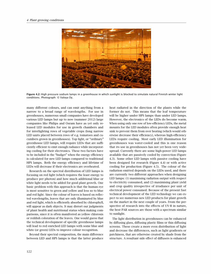
4 Plant growing conditions

Figure 4.2: High pressure sodium lamps in a greenhouse in which sunlight is blocked to simulate natural Finnish winter lightconditions. Photograph: © Valoya Oy.

many different colours, and can emit anything from anarrow to a broad range of wavelengths. For use ingreenhouses, numerous small companies have developedvarious LED lamps but up to now (summer 2012) largecompanies like Philips and Osram have as yet only re-leased LED modules for use in growth chambers andfor interlighting rows of vegetable crops (long narrowLED units placed between rows of e.g. tomatoes and cu-cumbers grown in greenhouses). Top light, or “ordinary”greenhouse LED lamps, will require LEDs that are suffi-ciently efficient to emit enough radiance while incorporat-ing cooling for their electronics. These two factors haveto be included in the “budget” when the energy efficiencyis calculated for new LED lamps compared to traditionalHPS lamps. Both the energy efficiency and lifetime ofLEDs will decrease if their electronics are overheated.

Research on the spectral distribution of LED lamps isfocusing on red light (which requires the least energy toproduce per photon) and how much additional blue orwhite light needs to be added for good plant growth. Onebasic problem with this approach is that the human eyeis most sensitive to green and yellow and less so to blueand red light. Since the colour of leaves is based on reflec-ted wavelengths, leaves that are only illuminated by blueand red light, which is efficiently absorbed by chlorophyll,will appear as dark objects. It may distort our judgmentsof plant health and nutritional status when making com-parisons, since it is often manifested as yellow chlorosisor reddish coloration of the leaves. One would guess thatthe technical development of specific greenhouse lampswill lead to red enriched LED lamps with some blue andwhite (or green) LEDs to improve colour recognition.

Beyond their spectral composition, the main differencebetween LED and HPS lamps is that the latter produce

heat radiated in the direction of the plants while theformer do not. This means that the leaf temperaturewill be higher under HPS lamps than under LED lamps.However, the electronics of the LEDs do become warm.When using only one row of low-efficiency LEDs, the metalmounts for the LED modules often provide enough heatsink to prevent them from over heating (which would oth-erwise decrease their efficiency), whereas high-efficiencyLEDs require cooling. Most early LED illumination forgreenhouses was water-cooled and this is one reasonthat its use in greenhouses has not yet been very wide-spread. Currently there are some high-power LED lampsavailable that are passively cooled by convection (Figure4.3). Some other LED lamps with passive cooling havebeen designed for research (Figure 4.4) or with activecooling for production (Figure 4.5). The colour of theradiation emitted depends on the LEDs used, and thereare currently two different approaches when designingLED lamps: (1) maximising radiation output with respectto electricity consumed, and (2) maximising plant yieldand crop quality irrespective of irradiance per unit ofelectrical power consumed. Because of the present fasttechnical development of the LED technology we can ex-pect to see numerous new LED products for plant growthon the market in the next couple of years. From the per-spective of research into the effects of UV-B in nature,the best PAR sources are those with a spectrum similarto sunlight.

The light distribution in greenhouses can be enhancedby diffusing glass, diffusing plastic films or thin diffusingscreens. These create a more even distribution of lightand decrease the differences, such as light gradients orpatchiness, that are otherwise created by shade from thestructure. A resultant side effect of diffusers is enhanced

122

4.2 Greenhouses

Figure 4.3: A comparison of the performance of two types of LED lamps with different emission spectra being used for thecultivation of an ornamental species (Kalanchoe). Photograph: © Valoya Oy.

Figure 4.4: Philips’ adjustable research modules with high efficiency LEDs: (A) white LEDs mounted in climate chamber (for whichthe research modules are designed) and (B) four modules used in a greenhouse (from left 40% blue in red, 20% blue in red, 100%red and white LEDs). In the climate chamber this setup of modules can be adjusted up to ca 300µmol m−2 s−1. Note that thewhite treatment looks brighter to the eye than the red and blue combinations, despite that all four colours give identical PPFD.Photograph: Eva Rosenqvist.

growth of plants due to better penetration of light intothe canopy (Markvart et al., 2010).

Commercially-available climate computers are oftenconnected to photometric (lux) sensors that measure lightvisible to humans (≈400–700 nm, see Box 1.1 on page6), whereas global radiation is measured radiometrically(W m−2, see Table 1.2 on page 5) in the range 400–1100or 400–3000 nm to provide information for the energy-related control of greenhouses (primarily temperature).The latter is the correct way to measure irradiance linkedto climate control; whereas visible light, related to pho-tosynthesis and plant production, should be measuredas PAR photon irradiance or photosynthetic photon fluxdensity (PPFD, µmol m−2 s−1, see Box 1.2 on page 7) orPAR (energy) irradiance (W m−2). Modern climate com-

puters can also be directly connected to PPFD sensors.

When using supplemental light from various lightsources extra care need to be taken on the choice ofquantum sensor since most supplemental greenhouselamps have a dis-continuous spectrum. Some cheaperquantum sensors do not cover the full spectral range400–700 nm and the sensor may not cover the spectrumof red LED’s, which can peak close to a wavelength of700 nm.

One should keep in mind, that moving an experimentfrom the field to a greenhouse does not make it independ-ent of the outdoor season, since the UV-B dose shouldbe balanced against the integrated daily PPFD if the ex-periment aims to mimic outdoor conditions. Daylightvaries tremendously between winter and summer. Even

123

4 Plant growing conditions

Figure 4.5: Top light LED lamps (Fionia Lighting, DK) tested for plant growth and energy consumption for light and greenhouseheating, in comparison with high pressure sodium lamps in the next greenhouse compartment. The setup gives supplementalPPFD of 120 µmol m−2 s−1 at a distance of 2.2 m from the bench, which is a level used for high light demanding species inproduction. Photograph: Carl-Otto Ottosen.

with supplemental light the PPFD of a sunny winter dayin Northern Europe will only correspond to an overcastday in the summer (Figure 4.1). The contribution fromlamps will be less than what is found in sunlight duringthe summer, even under long photoperiods (c.f. Figures4.6 and 4.1).

Except for late successional species that ecologicallyare adapted to obligate shade, most plants will acclimateto the prevailing light conditions (Bazzaz and Carlson,1982). This means changing chloroplast architecture andthe stoichiometry of the whole photosynthetic apparatus(Anderson et al., 1988) and thus also altering the lightresponse of photosynthesis.

Most experiments on light acclimation only discus thelight environment in terms of “high light” or “low light”,regardless if it has been created as % of sunlight withpermanent shade screens or as a certain PPFD in climatechambers. However, the light environment should bedescribed by day length, maximum PPFD and integrateddaily PPFD. Not much is known about which of the para-meters of the light environment, actually trigger accli-mation of photosynthesis. The three light parametersmentioned above have been investigated in tomato (Vanden Boogaard et al., 2001), where the day length affectedthe chlorophyll concentration while the integrated dailyPPFD affected the maximum rate of CO2 fixation at lightsaturation, independent of what the maximum PPFD wasduring the day.

If photosynthesis is being studied in greenhouses inrelation to UV-B one should be aware of the effect thatthe seasonal changes in daylight has on the photosyn-thetic apparatus and therefore also on the growth of the

plants, when comparing different experiments conductedat different times of the year.

4.2.3 Air humidity

Air humidity is difficult to regulate in greenhouses. If fewplants are grown in a compartment the humidity tends tobe low due to the large areas of potentially cold glass andconcrete that act as dehumidifiers through condensation.If the leaf area index (LAI) is high, transpiration will makehumidity correspondingly high despite condensation onthe greenhouse surfaces.

Misting systems can increase the humidity but it isimportant that they create mist, not rain. Rain or con-densation on the plants will increase the risk of fungaldisease in the experimental plants.

The humidity will be higher in highly insulated thanin single-glass greenhouses, where some of the humiditywill condense on the glass. High air humidity is decreasedby opening the vents at the same time as turning on theheating system to increase the exchange of air with theoutside. The effect of dehumidifying ventilation will de-pend on the outdoor weather conditions and on whetherdry or moist air is entering the greenhouse.

Using traditional climate control, the air humidity isregulated as relative humidity (RH, %). The driving forceof transpiration is the absolute gradient of water vapourfrom the intercellular spaces inside the leaf to the out-side air, i.e. the water vapour pressure difference (∆e,Pa). As the intercellular spaces are microscopic and thecell walls saturated with water it is assumed that the RHin the leaf is 100% at the given leaf temperature. Since

124

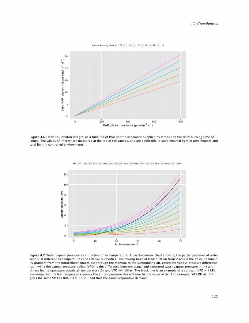
4.2 Greenhouses

0

10

20

30

40

50

0 200 400 600 800PAR photon irradiance (µmol m−2 s−1)

Dai

ly P

AR

pho

ton

inte

gral

(mol

m−2

d−1

)

Lamps burning time (h d−1) 10 12 14 16 18

Figure 4.6: Daily PAR photon integral as a function of PAR photon irradiance supplied by lamps and the daily burning time oflamps. The values of interest are measured at the top of the canopy, and are applicable to supplemental light in greenhouses andtotal light in controlled environments.

0

2

4

6

8

10

12

0 10 20 30 40 50Air temperature (C)

Vapo

ur p

ress

ure

(kPa

)

RH 10% 20% 30% 40% 50% 60% 70% 80% 90% 100%

Figure 4.7: Water vapour pressure as a function of air temperature. A psychrometric chart showing the partial pressure of watervapour at different air temperatures and relative humidities. The driving force of transpiration from leaves is the absolute humid-ity gradient from the intracellular spaces out through the stomata to the surrounding air, called the vapour pressure difference(∆e), while the vapour pressure deficit (VPD) is the difference between actual and saturated water vapour pressure in the air.Unless leaf temperature equals air temperature ∆e and VPD will differ. The black line is an example of a constant VPD = 1 kPa,assuming that the leaf temperature equals the air temperature this will also be the value of ∆e. For example, 50% RH at 15Cgives the same VPD as 80% RH at 32.5C and thus the same evaporative demand.

125

4 Plant growing conditions

the absolute content of water vapour in air of the sameRH is strongly temperature dependent (Figure 4.7), theevaporative demand can differ greatly when temperaturefluctuates in the greenhouse, even if RH is stable.

In modern climate computers a measured quantity equi-valent to VPD (i.e. based on absolute difference in humid-ity, expressed as water mass concentration, instead ofdifference in partial pressure) can be used for humiditycontrol, instead of RH. It is called delta-χ (∆χ, g m−3, orsometimes simply delta-X) and is the water deficit fromthe saturated value, but expressed based on mass concen-tration instead of vapour pressure. Both VPD and ∆χ usesaturated water vapour content based on air temperatureas a reference. To be correct we need information aboutthe canopy temperature to use VPD or ∆χ to estimatethe true evaporative demand (∆e) as when the leaves aretranspiring their temperature will be somewhat lowerthan the air temperature, due to evaporative cooling. Thecanopy temperature is not easily measured but in thecontext of climate control the approximation based ofVPD or ∆χ still provides a better approximation to thetrue evaporative demand created by the atmosphere inthe greenhouse than RH.

Misting systems using ultrasonic humidifiers have beenreported to also generate some hydrogen peroxide andmay not be appropriate in research studies of plantgrowth (Arends et al., 1988). Although the evidence is notstrong, one should be aware of this possible undesiredeffect.

However, increasing air humidity in greenhouses byforced aerosolization of water (creating small droplets bywater sprays, jets, ultrasonic nebulizers etc.) may causedifferent problems. These processes cause charge sep-aration of water droplets and thus forming high concen-trations of nano-sized ions, which can damage electronicequipment due to electrostatic deposition. The effects ofthe charged droplets on plants are not known. This effectis not seen if water is being evaporated directly from awater surface to water vapour e.g. by trickling water infans with cooling pads.

4.2.4 Elevated carbon dioxide concentration

Modern greenhouses have systems to supply elevatedCO2 concentration to promote crop growth. There areseveral possible sources of CO2 that can be used: thethree most common ones are liquid CO2 from a tank,combustion of natural gas for CO2 production and CO2

produced when burning fossil fuels for heat/power pro-duction, where the latter two require cleaning of thefumes to remove NOx and SOx.

A major difference between elevated CO2 supplied infull-scale greenhouses compared to open-top chambers

or FACE is that the greenhouse CO2 is not supplied con-tinuously during daytime hours. Because of the vastvolume of a greenhouse compartment it would be veryexpensive to supply elevated CO2 when the vents areopen for temperature control. Therefore in traditionalgreenhouse climate control elevated CO2 is given onlywhen the vents are closed or open by at most 5%. Ethyl-ene contamination, which can significantly reduce plantgrowth, has been reported in some CO2 supplies andit should be removed by KMnO4 scrubbing if necessary(Morison and Gifford, 1984).

Furthermore the isotope composition may differ inliquid CO2 compared to natural air, which need to bechecked if investigations include measurements of the13C/12C ratio e.g. in relation to water balance, and whencomparing with results in the literature.

4.2.5 Growth substrates, irrigation andfertilization

Transferring experiments indoors inevitably means grow-ing the plants in pots. It is important to chose a growthsubstrate that has both good water holding and drainingproperties to meet the demand for water and oxygen forthe root system. In the horticultural greenhouse industrypeat mixtures are the most commonly used substrate inpots but also coco-peat (granulated husks of coconuts)is used. To ensure good aeration perlite or vermiculiteis sometimes mixed into the substrate. Since the potvolume is limited the fluctuations in water content willbe greater than in soil, as will be the fluctuations in soiltemperature. In natural soil the temperature will be bothmore stable and lower than what it is in pots.

The pots are often of dark colour and they absorb heatradiation when exposed to sunlight. In commercial pro-duction the pot density is kept high enough to createshade between the pots and only the outer row of potsare potentially exposed to heat radiation from the sun.In experiments you often leave some space between theplants, not to have excessive shade between them. Dur-ing sunny days without shade the pot temperature caneasily increase to levels that are damaging to the rootsystem and when knocking the soil/root out of the pot ofborder plants that has been exposed to direct sunlight itis not uncommon to see root death on the exposed sideof the pot. The temperature of the nutrient solution/wa-ter also affects the root temperature. If the water is colda growth retarding effect can be seen on the plants. Morereflections on pot experiments are found in Passioura(2006) and a meta-analysis of the effect of pot size onplant growth in Poorter, Bühler et al. (2012).

Several types of watering systems exist but the mostcommon ones are drip irrigation and ebb/flow systems.

126

4.3 Open top chambers and FACE

Drip irrigation is based on thin tubes supplying each potwith nutrient solution from a tank. In an ebb/flow systemthe nutrient solution it pumped up on the bench to 1–2cm water depth and kept there for some minutes, beforebeing drained off, back into the tank. This system recir-culates the nutrient solution and with commercial nutri-ent/watering computers the composition is controlled bypH and electric conductivity (EC) of the solution, toppingup with stock solution or an acid to keep the nutrientconcentration and pH at desired level.

Irrigation of the plants can be done by timer or ondemand. In greenhouses plants will have different needfor water dependent on the weather. If the irrigation isdone by timer without adjustment for sunny or overcastweather there will be a risk that the plants are over-watered during dull days or water stressed on sunnydays. Both stresses potentially affect the growth of theplants.

Watering by demand can be done by experience or byweighing the plants and watering after a pre-determinedwater loss. Load cells can be mounted under ca. 0.5 m2

watering trays or under a section of a greenhouse bench,triggering a pump in the tank with nutrient solution viaa datalogger. Since plants that grow to maturity follow asigmoid growth curve the watering needs to be adjustedaccordingly during the experiment, to follow the demand.

4.2.6 Data logging of microclimatic variables

When working in greenhouses it is not enough to reportthe set points used for the most important climate para-meters. The climate in a greenhouse needs to be meas-ured and the observed values reported. The optimumarrangement is to have separate sensors recording theclimate to those that are controlling the climate, but ifthis is not possible the ones connected to the climatecomputer can be used, if they are calibrated. Light ir-radiance, air temperature and humidity are the mostimportant parameters to record, along with CO2 concen-tration if it is applied. Since the natural irradiance canfluctuate rapidly, it is important to have a high loggingfrequency, e.g. every minute. Furthermore, it is importantthat the temperature sensor is shielded from direct heatradiation from the sun and the lamps, while still beingexposed to free air, e.g. in a ventilated box. For ideason how to construct a radiation shield for measurementof air temperature refer to the design of weather sta-tions (e.g. http://www.kippzonen.com, http://www.skyeinstruments.com and may others).There are several small dataloggers on the market, withbuilt-in air temperature and humidity sensors in a plastichousing. They also have to be shielded from heat ra-diation when used in a greenhouse or climate chambersince the plastic housing gradually heats up and transfers

the body temperature to the sensor—in climate cham-bers with metal halide lamps errors larger than 10Chave been observed when no shielding was used. Recom-mendations for sensors and frequency of data loggingare compiled in Table 4.1.

4.3 Open top chambers and FACE

Open top chambers (OTC) and, less frequently, closed topchambers (CTC) are used to study the effects of elevatedCO2 concentration and temperature. Most of these cham-bers are built using plastic films, plates, or glass thatabsorb UV-B radiation and sometimes also some UV-Aradiation. In some cases, attenuation of UV radiationhas been minimised by use of UV-transparent materialsin OTCs and CTCs e.g. Visser et al., 1997. In contrast toOTCs and CTCs, free air CO2 enhancement (FACE) sys-tems do not significantly affect UV or visible radiation. Insome cases, UV-B lamps have been used in OTCs and theUV-B attenuation measured. In controls with unenergisedlamps, daily integrals of UV-B and UV-A radiation, andPAR were reduced by 24% (Booker et al., 1992).

4.4 Controlled environments

In controlled environments the spectral distribution ofthe light emitted by the lamps used is especially im-portant since there is no contribution from natural light.A skewed spectrum can cause strange growth patternsin plants and many lamp types produce distinct emis-sion bands, interrupted by bands of very low emission(Figure 4.8). Fluorescent tubes and HPS lamps, in par-ticular, emit very little far-red and produce plants withvery stunted growth, compared to lamps that create acontinuous spectrum resembling sunlight (Hogewoninget al., 2010). However, lamps emitting a continuous spec-trum can also create unexpected differences in plantscompared to sunlight. An unpublished example is that ofwhite cabbage grown in pots outdoors then moved into aclimate chamber with metal halide bulbs (see Figure 4.8),which developed a distinct red coloration after a coupleof hours at constant light.

UV-B lamps emit some blue light providing a weakvisual indicator that the lamp is turned on, but the contri-bution to the light environment will be minor in compar-ison to the overall PPFD from the main lamps used forPAR. They also emit very small amounts of orange-redradiation.

Most lamps presently used also emit a substantialamount of heat radiation. Some of this heat should beremoved using a heat filter. The most efficient designto achieve this is to have the lamps in a separate, ventil-ated compartment in the ceiling, divided from the growth

127

4 Plant growing conditions

Tab

le4

.1:G

uid

elines

for

describ

ing

gro

wth

conditio

ns

inco

ntro

lleden

vironm

ents

and

green

houses,

based

on

the

recom

men

datio

ns

of

The

Intern

ational

Com

mittee

for

Contro

lledEn

vironm

ent

Guid

elines

(http://www.controlledenvironments.org/

)on

which

param

eterssh

ould

be

record

edfo

rpro

per

descrip

tion

of

conditio

ns

inclim

atech

ambers.

We

have

modifi

edit

slightly

and

added

recom

men

datio

ns

for

measu

remen

tsin

green

houses

(for

the

climate

param

etersalso

validfo

rth

em).

Ingreen

houses

and

inth

efi

elda

data

logger

with

temperatu

re,PA

Ran

dhum

idity

senso

rsis

required

.n.a.:

not

applicab

le.

Param

eterU

nits

Wh

ereto

measu

reW

hen

tom

easure

Wh

atto

report

Clim

atech

amb

erG

reenh

ou

se

Rad

iation

PPFD

µm

olm−

2s −

1T

op

of

the

canop

yin

the

centre

of

gro

win

garea

(ingreen

hou

ses>

1sen

sor

isp

referred)

Start,every

2w

eeks

and

end

of

experim

ent

n.a.

Mean

(daytim

e)an

ds.d

.R

adiatio

nso

urce

(type,m

od

el,man

ufactu

rer)

PPFD

µm

olm−

2s −

1A

sab

ove

n.a.

Loggin

gevery

min

ute

Mean

max.

daily

PA

Ran

ds.d

.M

eanin

-teg

ratedPA

Ran

ds.d

..R

adiatio

nso

urce

(type,m

od

el,man

ufactu

rer)Ph

oto

perio

dh

n.a.

n.a.

n.a.

Du

ration

of

ligh

tan

dd

arkp

eriod

(ingreen

hou

sefo

rstart

and

end

of

experi-

men

t).

Tem

peratu

reA

irC

Top

of

canop

yin

the

centre

of

gro

win

garea

Daily

du

ring

eachlig

ht

and

dark

perio

d,

atleast

1h

afterlig

ht/d

arkch

ange

Loggin

gevery

1–5

min

utes

Mean

and

s.d.

for

day

and

nig

ht

tem-

peratu

re,sp

ecificatio

nif

itd

oes

not

follo

wth

ep

hoto

perio

d.

Air

hu

mid

ityW

atervap

ou

rp

res-su

red

eficit

(VPD

)kPa

Top

of

canop

yin

the

centre

of

gro

win

garea

As

for

airtem

peratu

reLo

ggin

gevery

1–5

min

utes

Averag

ean

dstan

dard

deviatio

n

∆χ

gm−

3A

sab

ove

As

above

As

above

As

above

Relative

hu

mid

ity%

As

above

As

above

As

above

As

above

(on

lyif

VPD

or∆χ

not

avail-ab

le)

Carb

on

dio

x-id

eIf

elevatedan

dp

artof

the

treatmen

tµ

molm

ol −

1T

op

of

canop

yA

tleast

hou

rlyLo

ggin

gevery

1–5

min

utes

(viaclim

ateco

mp

uter)

Mean

and

s.d.

Air

velocity

Ifavailab

lean

dp

artof

the

treat-m

ent

ms −

1A

ton

eor

more

repres-

entative

canop

ylo

ca-tio

ns

At

leaston

ced

urin

gth

eexp

erimen

tM

eanan

ds.d

.

Sub

straten

.a.n

.a.n

.a.A

tstart

of

experim

ent

At

startof

ex-p

erimen

tT

ype

and

volu

me

per

con

tainer,

com

-p

on

ents

of

soil(-less)

sub

strate,co

n-

tainer

dim

ensio

ns

Waterin

gn

.a.l

(litre)n

.a.D

ailyD

ailyFreq

uen

cy,am

ou

nt

and

type

of

water

add

edN

utritio

nor

liqu

idcu

lture

Acid

ityp

HIn

bu

lkso

lutio

nB

efore

and

afterp

Hco

rrection

Befo

rean

dafter

pH

cor-

rection

Mean

and

s.d.

Electric

con

du

ctiv-ity

(EC)

Sm−

1A

sab

ove

Befo

rean

dafter

EC

correctio

nB

efore

and

afterEC

cor-

rection

Averag

ean

dstan

dard

deviatio

n

Ion

com

positio

nm

moll −

1A

sab

ove

Daily

or

wh

enrep

len-

ished

Daily

or

wh

enrep

lenish

edIo

nic

con

centratio

nin

initial

and

add

edso

lutio

n.

Aeratio

nif

any.

Volu

me

of

initial

solu

tion

.So

lidm

edia

molk

g −1

n.a.

Wh

enad

ded

or

replen

-ish

edW

hen

add

edor

replen

ished

Nu

trients

and

their

form

add

edto

soil

med

ia.

128

4.5 Material issues in greenhouses and controlled environments

chamber by a transparent glass/plexi-glass sheet. Evenso, it is important that the temperature sensor meas-uring air temperature in a climate chamber is shieldedfrom the heat radiation from the lamps. Water is a goodabsorber of infra-red radiation, and sometimes a trans-parent tray with circulating water2 is used as a barrierbetween lamps and the plant compartment. Most lamptypes (e.g. metal halide) used in climate chambers canonly be turned on/off, not dimmed. To create differentphoton irradiances the lamps has to be turned on in dif-ferent constellations. Even though daylight shows strongand fast variations in irradiance (Figure 4.10 on page 132)the overall light pattern is bell shaped. To mimic naturallight conditions a gradual or stepwise change during themorning/evening hours is preferred. If it is possible toget e.g. 600 µmol m−2 s−1 from the lamps, a 14 h-longday will give an integrated PPFD of 30 mol m−2 d−1, whichcorresponds to a sunny day in May in Denmark (Figures4.1 and 4.6). With the present development of the LEDtechnology the first climate chambers with LED lightinghave been introduced to the market, and one can expectthat LEDs will be used extensivelly for controlled envir-onments in the future. LEDs can be dimmed withoutany drastic changes in their spectral profile and the lackof heat radiation in the direction of the plants removesone complicating factor for lighting in climate chambers.Figure 4.8 shows the photon emission spectra of somelamps used as PAR sources in controlled environmentsand greenhouses.

In climate chambers it is often possible to create a fastchange between the day and night temperatures, thoughthis is unnatural to plants. Under natural conditions a5–10C decrease in air temperature normally takes hours,allowing e.g. the membrane fluidity to follow. If the tem-perature drop between day and night is big and fast someplants may experience transient stress linked to mem-brane fluidity, which would not be the case if the changewere slower. This is something to bear in mind, whendesigning the chamber climate. It can also increase therisk of fungal disease if the air humidity is high and theplants become damp, in the same way as in greenhouses.

If experiments are done at low or high temperaturesthere may be restrictions on how well humidity can becontrolled. At low temperature there may be limitationson the capacity for dehumidification and at high temper-atures it may not be possible to sufficiently moisten theair.

Numerous plant species lose the ability to effectivelyregulate their stomata when grown at constant high hu-midity (ca. 70% RH at 20–25C). To our knowledge, thishas been observed in Helianthus annuus, Lycopersicon es-culentum, Cucumis sativus and Gerbera × hybrida. These

plants lose their ability to regulate stomatal conductancewhen subsequently exposed to low air humidity e.g. ifmoved from the greenhouse to a laboratory for measure-ments of photosynthesis. In the worse case scenarios, theplants transpire to such an extent that small local spotsof necrosis develop on the patch where gas exchange hasbeen measured on the leaf. However, since results likethese are considered as failed experiments such obser-vations have not (to our knowledge) been scientificallypublished. Nevertheless, it is important to be aware ofthis potential problem when working with mesophyticleaves, i.e. “average” leaves that are adapted neither todry nor to wet conditions, like the examples above.

Data logging of the climate is needed in controlledenvironments to catch irregularities and failings in theclimate control. This is especially important to test fordifferences among chambers when the climate set pointschanges. The Committee on Controlled EnvironmentTechnology and Use under the USDA has issued recom-mendations for data logging of growth chamber climate,which are compiled, with some changes, in Tables 4.1and 4.2.

Recommendations on parameters that should belogged have been published by the International Commit-tee for Controlled Environment Guidelines - see http://www.controlledenvironments.org/,http://www.ceug.ac.uk/ICCEG.htm andhttp://www.controlledenvironments.org/guidelines.htm.

4.5 Material issues in greenhouses andcontrolled environments

A potentially problematic issue concerning materials ingreenhouses and climate chambers relates to the use ofdifferent types of soft plastic materials. Plastics like cellu-lose acetate, cellulose nitrate or PVC are stiff by nature. Itis only when they are mixed with a softener i.e. a “plasti-ciser” that they become soft and flexible. The plasticisersmay be different alkyl esters of phthalic acid. Some ofthese phthalates are phytotoxic, particularly butyl phthal-ate (DBP) and di-isobutyl phthalate (DIBP) (Hannay andMillar, 1986; Millar and Hannay, 1986). The phytotoxicityis evident as poor growth, chlorosis, necrosis and plantdeath. At regular intervals since the 1950’s there havebeen examples in the greenhouse industry and plant re-search facilities where new plastics have been introducedfor different purposes, which have caused serious growthproblems (Hardwick and Cole, 1987). Many species aredamaged by phthalates but species of Brassicaceae seemto be particularly sensitive. Past examples of productsresponsible for phytotoxic problems include plastic tun-

2Circulation or cooling of the water is needed to remove the heat from the system, otherwise the water could even boil.

129

4 Plant growing conditions

A: Fluorescent 1 B: Fluorescent 2

C: Fluorescent 3 D: Incandescent

E: Metal halide F: Sodium (HPS)

0.0

0.2

0.4

0.6

0.00

0.05

0.10

0.15

0.20

0

1

2

3

0.0

0.5

1.0

0

2

4

6

012345

300 400 500 600 700 800 900 300 400 500 600 700 800 900Wavelength (nm)

Spe

ctra

l irr

adia

nce

(µm

ol m

−2 s

−1 n

m−1

)

Figure 4.8: Photon emission spectra of visible light emitting lamps commonly used as PAR sources in controlled environments.A: T8 fluor. tube ‘cool daylight’ 36 W Philips TL‘D’ 36W/865; B: T8 fluor. tube ‘incandescent’ 36 W Philips TL‘D’ 36W/92; C:T12 fluor. VHO ‘cool white’ 215 W Sylvania F96T12/CW/VHO; D: 60 W incandescent lamp; E: Osram HQI 400 W/D metal halidedischarge lamps; F: Osram NAV-T400 high pressure sodium lamp. Lamps have been measured individually and in banks, and thedistance to the spectroradiometer differs, meaning that absolute spectral photon irradiances are not comparable between panels.Measured with a LI-1800 spectroradiometer (LI-COR, Lincoln, NE, USA).

Table 4.2: Guidelines for describing controlled environments and greenhouses. n.a.: not applicable.

Parameter Units What to report

Manufacturer n.a. Name and address (n.a. for greenhouse)

Model n.a. Model descriptor if available. Greenhouse type and roof height for green-houses

Size m2 Floor area

Barrier beneath lamps Yes/No Indicate if present and composition. Optical properties if available (notgreenhouses)

Cladding material n.a. Indicate material and optical properties if known (only for greenhouses)

Air flow n.a. Indicate whether up, down or horizontal (not greenhouses)

130

4.6 Gas-exchange cuvettes and chambers

nels, water hoses, drip irrigation tubes, plastic plant pots,glazing strips (that seal between the glass and aluminiumframes in the greenhouse construction), plastic insulationof electrical wires and plastic boots—the latter creatinggrowth problems in a greenhouse outside a staff chan-ging room. Many of these problems have been createdwhen the recipes or composition of products already inuse in a greenhouse have been changed by the manufac-turer. Growth chambers require some fresh air inlet forthe climate control. There is an example of poor growthand bleaching of plants in a climate chamber when theair inlet was close to the ventilation outlet of a chemistrylaboratory. When the air inlet was moved 200 m away andsupplied with a compressor, the problem disappeared.

4.6 Gas-exchange cuvettes and chambers

Measurement of photosynthesis through gas-exchangewith UV-B present requires modifications of most stand-ard equipment. Most gas-exchange cuvettes have win-dows that attenuate UV radiation. This means that mostleaf photosynthesis and stomatal conductance measure-ments are done in the absence of UV radiation, even whendone in sunlight. Stomata have been shown to respondto UV radiation (e.g. Eisinger et al., 2000), and at highUV irradiances the rate of photosynthesis can also beaffected (see Rozema et al., 1997, for a consice review).

For example, the GFS-3000 system from Walz, can beordered with cuvette windows made of quartz instead ofnormal glass. Some cuvettes for the LI-COR LI-6400 usea plastic film as a window, and it is possible to use anUV-transparent material. The cuvette for CIRAS-2 fromPP Systems is delivered with Calflex heat filter glass asstandard, but can easily be fitted with quartz glass forUV-B transmission on request.

Frequently used light sources are tungsten-halogenlamps, which emit very little UV radiation, or lightsources based on red LEDs in combination with blueor white LEDs, which do not emit any UV-B radiation.

When designing experiments, especially when leaves orshoots are enclosed for more than a couple of minutesin a gas-exchange cuvette, one should be aware that theleaves or shoots may be in an unnatural light environ-ment, even when measurements are done in full sunshine.To avoid surprises, always measure irradiance and espe-cially spectral irradiance through the cuvette window,rather than outside the cuvette, if you want to describethe radiation environment during measurements.

Plastic and rubber used for tubing have different prop-erties of permeability to CO2 and water vapour, and ab-sorption of water, which can lead to flawed gas-exchangedata. These properties are listed in Long and Hällgren(1987).

4.7 Plants in the field

One important disturbance in experiments on naturalvegetation or field crops is that produced by the research-ers themselves. Some ecosystems like peat bogs getmore easily damaged than others, but in most cases spe-cial precautions are needed whenever repeated accessto plots is needed. The most common approach is touse catwalks made from wooden planks raised some cen-timetres above the ground. Sometimes when access isneeded to the centre of the plots ladders are put tempor-arily, laying horizontally bridging two catwalks. Figure4.9 shows some examples from Abisko and Figure 2.24on page 56 shows an example from Ushuaia.

Not only the spectrum, but also the temporal variationof irradiance differs between controlled environmentsand natural conditions. The temporal light regime de-pends on the position of the sun and on clouds (Figure4.10), and also on the vegetation itself (Figure 4.11). Forexperiments done in the field summaries of data froman in situ or nearby weather station should be used todescribe the growing conditions. To assess the light en-vironment at different locations in a forest understorey,hemispherical photographs taken with a fish-eye lens,can be used. There is software available—e.g. Hemiviewfrom Delta-T—that allows the prediction of the light en-vironment based on the position of the sun in the sky atdifferent times of the day and seasons of the year.

4.8 Cultivation of aquatic plants

When designing experimental set ups for the cultivationof aquatic plants under full solar radiation (PAR + UV-A+ UV-B) or under a simulated natural radiation field (seesection 2.4 on page 62), the spectral transmission of thevessels or photobioreactors used must be accounted foras well as the absorbtion of UV radiation by the water,growth medium and the aquatic plants themselves (selfshading). Most studies evaluating photosynthetic activityin algae have been conducted in UV-opaque incubatorsand this has consequently led to overestimation of theirphotosynthetic capacity, since UV radiation causes pho-toinhibition and photodamage in aquatic plants (Bischofet al., 2006; Häder and Figueroa, 1997; Villafañe et al.,2003).

The most frequently used photobioreactors have a cyl-indrical shape and they can be transparent or opaque toUV radiation (Figure 4.12, see section 2.4 on page 62).Some photobioreactors are built from rigid plastic suchas polycarbonate (PC), polymethylmethacrylate (PMM) orpolyvinyl chloride (PVC), and others from flexible plasticsuch as cellulose acetate or polyethylene.

The aims of photobioreactor design are: (a) high volu-

131

4 Plant growing conditions

Figure 4.9: View of two UV-B experiments in Abisko, Sweden, showing the use of catwalks to protect the natural vegetation understudy. Left: use of small UV-B lamps on small plants; Dr. Carlos L. Ballaré. Right: Use of frames with 40W UV-B lamps; Prof. LarsOlof Björn. Photographs: Pedro J. Aphalo.

130 131 132 133

134 135 136 137

138 139 140 141

142 143 144 145

0500

100015002000

0500

100015002000

0500

100015002000

0500

100015002000

00:00 12:00 00:00 12:00 00:00 12:00 00:00 12:00Time of day (h)

PA

R p

hoto

n irr

adia

nce

(µm

ol m

−2 s

−1)

Figure 4.10: The effect of clouds on light regime. Total (red) and diffuse (blue) PAR photon irradiance throughout 16 Spring days,starting from day 130 or 9 May 2012, in Viikki, Helsinki, Finland. Measured with a BF5 instrument (Delta-T, Cambridge, U.K.) anda CR10X datalogger (Campbell Scientific, Ltd, Logan, Utah, U.S.A.). Plotted data are one minute averages. Panel headings indicatethe day of year. Unpublished data: Pedro J. Aphalo, T. Matthew Robson, Oriane Loiseau and Saara Hartikainen.

132

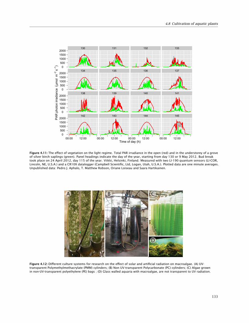
4.8 Cultivation of aquatic plants

130 131 132 133

134 135 136 137

138 139 140 141

142 143 144 145

0500100015002000

0500100015002000

0500100015002000

0500100015002000

00:00 12:00 00:00 12:00 00:00 12:00 00:00 12:00Time of day (h)

PA

R p

hoto

n irr

adia

nce

(µm

ol m

−2 s

−1)

Figure 4.11: The effect of vegetation on the light regime. Total PAR irradiance in the open (red) and in the understorey of a groveof silver birch saplings (green). Panel headings indicate the day of the year, starting from day 130 or 9 May 2012. Bud breaktook place on 24 April 2012, day 115 of the year. Viikki, Helsinki, Finland. Measured with two LI-190 quantum sensors (LI-COR,Lincoln, NE, U.S.A:) and a CR10X datalogger (Campbell Scientific, Ltd, Logan, Utah, U.S.A.). Plotted data are one minute averages.Unpublished data: Pedro J. Aphalo, T. Matthew Robson, Oriane Loiseau and Saara Hartikainen.

A B C

D

Figure 4.12: Different culture systems for research on the effect of solar and artificial radiation on macroalgae. (A) UV-transparent Polymethylmethacrylate (PMM) cylinders; (B) Non UV-transparent Polycarbonate (PC) cylinders; (C) Algae grownin non-UV-transparent polyethylene (PE) bags ; (D) Glass walled aquaria with macroalgae, are not transparent to UV radiation.

133

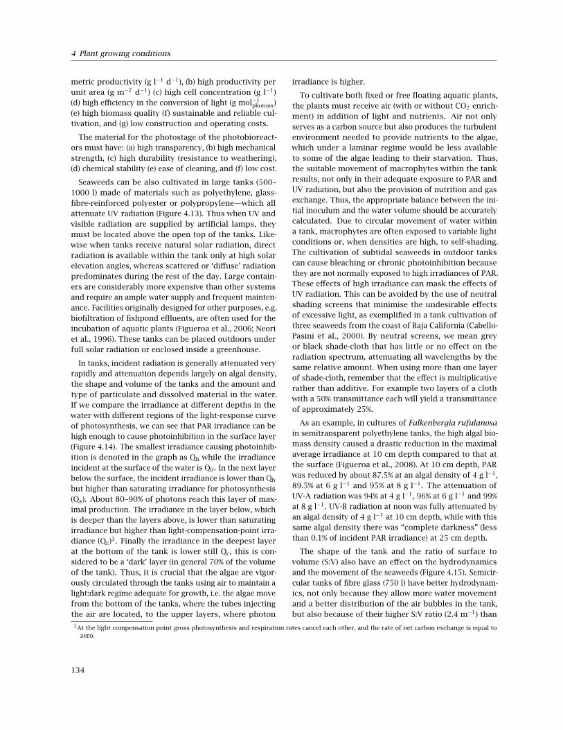
4 Plant growing conditions

metric productivity (g l−1 d−1), (b) high productivity perunit area (g m−2 d−1) (c) high cell concentration (g l−1)(d) high efficiency in the conversion of light (g mol−1

photons)(e) high biomass quality (f) sustainable and reliable cul-tivation, and (g) low construction and operating costs.

The material for the photostage of the photobioreact-ors must have: (a) high transparency, (b) high mechanicalstrength, (c) high durability (resistance to weathering),(d) chemical stability (e) ease of cleaning, and (f) low cost.

Seaweeds can be also cultivated in large tanks (500–1000 l) made of materials such as polyethylene, glass-fibre-reinforced polyester or polypropylene—which allattenuate UV radiation (Figure 4.13). Thus when UV andvisible radiation are supplied by artificial lamps, theymust be located above the open top of the tanks. Like-wise when tanks receive natural solar radiation, directradiation is available within the tank only at high solarelevation angles, whereas scattered or ‘diffuse’ radiationpredominates during the rest of the day. Large contain-ers are considerably more expensive than other systemsand require an ample water supply and frequent mainten-ance. Facilities originally designed for other purposes, e.g.biofiltration of fishpond effluents, are often used for theincubation of aquatic plants (Figueroa et al., 2006; Neoriet al., 1996). These tanks can be placed outdoors underfull solar radiation or enclosed inside a greenhouse.

In tanks, incident radiation is generally attenuated veryrapidly and attenuation depends largely on algal density,the shape and volume of the tanks and the amount andtype of particulate and dissolved material in the water.If we compare the irradiance at different depths in thewater with different regions of the light-response curveof photosynthesis, we can see that PAR irradiance can behigh enough to cause photoinhibition in the surface layer(Figure 4.14). The smallest irradiance causing photoinhib-ition is denoted in the graph as Qh while the irradianceincident at the surface of the water is Q0. In the next layerbelow the surface, the incident irradiance is lower than Qh

but higher than saturating irradiance for photosynthesis(Qs). About 80–90% of photons reach this layer of max-imal production. The irradiance in the layer below, whichis deeper than the layers above, is lower than saturatingirradiance but higher than light-compensation-point irra-diance (Qc)3. Finally the irradiance in the deepest layerat the bottom of the tank is lower still Qc, this is con-sidered to be a ‘dark’ layer (in general 70% of the volumeof the tank). Thus, it is crucial that the algae are vigor-ously circulated through the tanks using air to maintain alight:dark regime adequate for growth, i.e. the algae movefrom the bottom of the tanks, where the tubes injectingthe air are located, to the upper layers, where photon

irradiance is higher.

To cultivate both fixed or free floating aquatic plants,the plants must receive air (with or without CO2 enrich-ment) in addition of light and nutrients. Air not onlyserves as a carbon source but also produces the turbulentenvironment needed to provide nutrients to the algae,which under a laminar regime would be less availableto some of the algae leading to their starvation. Thus,the suitable movement of macrophytes within the tankresults, not only in their adequate exposure to PAR andUV radiation, but also the provision of nutrition and gasexchange. Thus, the appropriate balance between the ini-tial inoculum and the water volume should be accuratelycalculated. Due to circular movement of water withina tank, macrophytes are often exposed to variable lightconditions or, when densities are high, to self-shading.The cultivation of subtidal seaweeds in outdoor tankscan cause bleaching or chronic photoinhibition becausethey are not normally exposed to high irradiances of PAR.These effects of high irradiance can mask the effects ofUV radiation. This can be avoided by the use of neutralshading screens that minimise the undesirable effectsof excessive light, as exemplified in a tank cultivation ofthree seaweeds from the coast of Baja California (Cabello-Pasini et al., 2000). By neutral screens, we mean greyor black shade-cloth that has little or no effect on theradiation spectrum, attenuating all wavelengths by thesame relative amount. When using more than one layerof shade-cloth, remember that the effect is multiplicativerather than additive. For example two layers of a clothwith a 50% transmittance each will yield a transmittanceof approximately 25%.

As an example, in cultures of Falkenbergia rufulanosain semitransparent polyethylene tanks, the high algal bio-mass density caused a drastic reduction in the maximalaverage irradiance at 10 cm depth compared to that atthe surface (Figueroa et al., 2008). At 10 cm depth, PARwas reduced by about 87.5% at an algal density of 4 g l−1,89.5% at 6 g l−1 and 95% at 8 g l−1. The attenuation ofUV-A radiation was 94% at 4 g l−1, 96% at 6 g l−1 and 99%at 8 g l−1. UV-B radiation at noon was fully attenuated byan algal density of 4 g l−1 at 10 cm depth, while with thissame algal density there was “complete darkness” (lessthan 0.1% of incident PAR irradiance) at 25 cm depth.

The shape of the tank and the ratio of surface tovolume (S:V) also have an effect on the hydrodynamicsand the movement of the seaweeds (Figure 4.15). Semicir-cular tanks of fibre glass (750 l) have better hydrodynam-ics, not only because they allow more water movementand a better distribution of the air bubbles in the tank,but also because of their higher S:V ratio (2.4 m−1) than

3At the light compensation point gross photosynthesis and respiration rates cancel each other, and the rate of net carbon exchange is equal tozero.

134

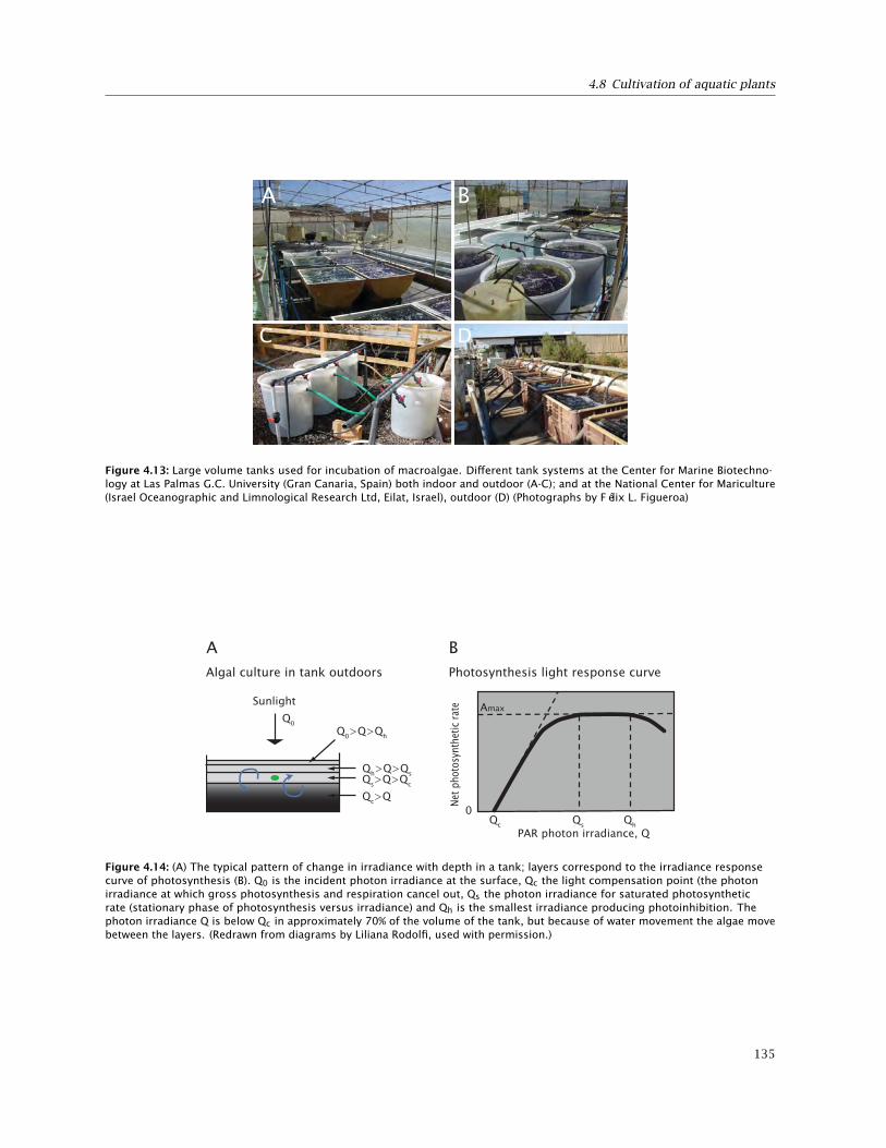
4.8 Cultivation of aquatic plants

A B

C D

Figure 4.13: Large volume tanks used for incubation of macroalgae. Different tank systems at the Center for Marine Biotechno-logy at Las Palmas G.C. University (Gran Canaria, Spain) both indoor and outdoor (A-C); and at the National Center for Mariculture(Israel Oceanographic and Limnological Research Ltd, Eilat, Israel), outdoor (D) (Photographs by Félix L. Figueroa)

Q0>Q>Qh

Qh>Q>QsQs>Q>Qc

Qc>Q

Photosynthesis light response curve

PAR photon irradiance, QQs Qh

Net p

hoto

synt

hetic

rate Amax

Qc

A BAlgal culture in tank outdoors

Sunlight

0

Q0

Figure 4.14: (A) The typical pattern of change in irradiance with depth in a tank; layers correspond to the irradiance responsecurve of photosynthesis (B). Q0 is the incident photon irradiance at the surface, Qc the light compensation point (the photonirradiance at which gross photosynthesis and respiration cancel out, Qs the photon irradiance for saturated photosyntheticrate (stationary phase of photosynthesis versus irradiance) and Qh is the smallest irradiance producing photoinhibition. Thephoton irradiance Q is below Qc in approximately 70% of the volume of the tank, but because of water movement the algae movebetween the layers. (Redrawn from diagrams by Liliana Rodolfi, used with permission.)

135

4 Plant growing conditions

A B C

Figure 4.15: Examples of tanks used for experiments with macroalgae, (a) semicircular tank of 750 l surface/volume ratio (S/V)=2.4 m−1 , (b) circular tank of 1500 l of capacity , S/V ratio=1 m−1 and (c) circular tank of 90 l , S/V =2.2 m−1).

that of cylindric 1500 l tanks of semitransparent poly-ethylene (S:V = 1 m−1) or 90 l (S:V = 2.2 m−1).

Another aspect of good experimental design is choos-ing the location of plants within the culture system, i.e.the merits of fixed- versus free-floating aquatic plants.Both fixed and free floating aquatic plants absorb radi-ation to differing extents depending on their pigmentcomposition and the thickness of their tissue or thallus.Aquatic angiosperms can be anchored to both naturalmaterials, such as stones, and artificial materials (rows,epoxy, etc.). Seaweeds are usually cultured in free float-ing systems where they are moved by the injection of air,although in nature they are fixed to different substrates.Not all species can be cultivated floating freely and insome cases this can alter their growth forms, transform-ing branched forms into a spherical forms. Morphologicalchanges affect both bio-optical properties (i.e. includingUV absorption) and nutrient assimilation which is higherin branched forms than spherical forms due to theirhigher surface:volume ratio (of both cells and the wholeplant). Thus, in photobiological experiments, it is crucialto optimise both algal density and the light field—by us-ing lamps located to one side (lateral position) or abovethe aquarium—so as to reduce or avoid self shading.

Mesocosms have been developed to recreate naturalconditions as closely as possible on a small scale. Theyare generally used to study plankton communities, how-ever, their use in aquatic macrophyte ecology is increas-ing. For example, floating mesocosms and mesocosmsconnected to land—e.g. attached to a platform or pier—have been developed (Figure 4.16).

Several mesocosm studies have used ambient radi-ation supplemented with UV-B radiation from fluores-cent lamps to simulate an increase in UV-B radiation dueto ozone depletion. Two methodologies can be applied:(a) supplementing a fixed irradiance value (“square wavesystems”), or (b) supplementing a fixed percentage ofambient irradiance (“modulated systems”) (Belzile et al.,

2006; Belzile et al., 1998). Modulated systems, which wereoriginally developed for terrestrial plants (Caldwell et al.,1983), are better than square-wave systems for simulat-ing predicted increases in UV radiation (S. Díaz et al.,2006, 2003). See section 2.2.6 on page 48.

When using mesocosms, experimental designs mustbe as realistic as possible in simulating forcing factorsas well as their variability. For example, when studyingthe effect of increased UV, experiments should be de-signed to reproduce diurnal variations in irradiance andepisodic events such as passing clouds. Recently, experi-ments using mesocosms have been applied to evaluatethe interactive effects on macrophytes of environmentalshifts driven by climate changes (temperature, PAR, UVradiation and nutrient availability). To mimic climatechange conditions, Liboriussen et al. (2005) designeda flow-through mesocosm in a shallow lake which canalso be applied to other aquatic ecosystems. Recently, anew automatically-operated system providing accuratesimulations of the increases in UV-B radiation and tem-perature according to climate change scenarios has beendeveloped (Nouguier et al., 2007). All these systems repro-duce the sort of high degree of environmental variabilityinherent to aquatic systems.

4.9 Recommendations

In this section we list recommendations related to thecultivation of plants used in experiments studying theeffects of UV radiation. See sections 2.6.1 and 2.6.2 forrecommendations on manipulation of UV radiation, sec-tion 3.15 for recommendations on how to quantify UVradiation, and section 5.12 for recommendations aboutstatistical design of experiments.

1. Include in the methods description in your pub-lications enough information about the growing

136

4.9 Recommendations

A

B

Figure 4.16: (A-B) Free-floating mesocosms of the Helmholtz Centre for Ocean Research Kiel (GEOMAR), Germany and (C) meso-cosms attached to a platform in Espeland Marine Biological Station, Bergen, Norway. Photos: (A) Ulf Riebesell, GEOMAR; (B) JensChristian Nejstgaard, University of Bergen.

conditions so that the experiment can be duplic-ated.

2. When using growth chambers, growth rooms, orgreenhouses with environmental control systemsreport in addition to model and manufacturer andits address, all the settings used:

a) Temperature i. Day temperature (C) ii. Nighttemperature (C) iii. The temperature ramp(C h−1) used when increasing/decreasing thetemperature. (This function is important indecreasing the risk of fungal disease due tomoist plants, i.e. a too steep temperaturedrop will increase the risk of condensation onthe plants.) iv. Temperature when ventilation

starts (C) v. Temperature when ventilationstops (C) vi. Light-dependent temperature in-crease, if dynamic climate is applied

b) Air humidity i. Upper limit of humidity wherehumidity control starts

c) Lamps. i. Indicate type, and manufacturer,power rating. For rooms and chambers in-dicate whether they are separated from theplants by a barrier made of glass, acrylic,polycarbonate, or some other material. ii. Forgreenhouses indicate the ambient light setpoint when the lamps are turned on, and theambient light set point when the lamps areturned off. iii. The global radiation (W m−2)

137

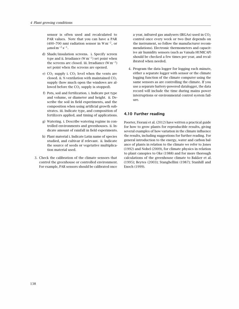
4 Plant growing conditions

sensor is often used and recalculated toPAR values. Note that you can have a PAR(400–700 nm) radiation sensor in W m−2, orµmol m−2 s−1.

d) Shade/insulation screens. i. Specify screentype and ii. Irradiance (W m−2) set point whenthe screens are closed. iii. Irradiance (W m−2)set point when the screens are opened.

e) CO2 supply i. CO2 level when the vents areclosed. ii. % ventilation with maintained CO2

supply (how much open the windows are al-lowed before the CO2 supply is stopped).

f) Pots, soil and fertilization. i. Indicate pot typeand volume, or diameter and height. ii. De-scribe the soil in field experiments, and thecomposition when using artificial growth sub-strates. iii. Indicate type, and composition offertilizers applied, and timing of applications.

g) Watering. i. Describe watering regime in con-trolled environments and greenhouses. ii. In-dicate amount of rainfall in field experiments.

h) Plant material i. Indicate Latin name of speciesstudied, and cultivar if relevant. ii. Indicatethe source of seeds or vegetative multiplica-tion material used.

3. Check the calibration of the climate sensors thatcontrol the greenhouse or controlled environment.For example, PAR sensors should be calibrated once

a year, infrared gas analysers (IRGAs) used in CO2

control once every week or two (but depends onthe instrument, so follow the manufacturer recom-mendations). Electronic thermometers and capacit-ive air humidity sensors (such as Vaisala HUMICAP)should be checked a few times per year, and recal-ibrated when needed.

4. Program the data logger for logging each minute,either a separate logger with sensor or the climatelogging function of the climate computer using thesame sensors as are controlling the climate. If youuse a separate battery-powered datalogger, the datarecord will include the time during mains powerinterruptions or environmental control system fail-ure.

4.10 Further reading

Poorter, Fiorani et al. (2012) have written a practical guidefor how to grow plants for reproducible results, givingseveral examples of how variation in the climate influencethe results, including suggestions for further reading. Forgeneral introduction to the energy, water and carbon bal-ance of plants in relation to the climate we refer to Jones(1992) and Nobel (2009), for climate physics in relationto plant canopies to Oke (1988) and for more thoroughcalculations of the greenhouse climate to Bakker et al.(1995); Beytes (2003); Stanghellini (1987); Stanhill andEnoch (1999).

138

5 Statistical design of UV experiments

Pedro J. Aphalo, T. Matthew Robson, Harri Högmander

5.1 Tests of hypotheses and model fitting

The guidelines given here for good experimental designhave been formulated with particular consideration givento UV manipulation experiments. Nevertheless most ofthe principles behind these guidelines can be generallyapplied to the design of experiments.

Experiments can be designed to test hypotheses or toestimate the values of parameters in a model. In the firstcase, we should be careful not to let our knowledge ofthe data influence the tested hypothesis1. In the secondcase, model choice may to some extent depend on thedata, but we should be aware that this a posteriori choiceof a functional relationship, could make the P -values lessstrict for testing treatment effects.

Fitting models is especially useful when the parametersof the model have a biological interpretation. In this case,it is important to obtain estimates of the reliability ofyour estimates of the values obtained for the parameters.In other words, we need to present not only the fittedvalues, but also their confidence intervals, or at leaststandard deviations.

All estimates of P -values are based on a comparisonof the variation between differently treated experimentalunits, and the variation among equally treated experi-mental units2. If we assign treatments objectively byrandomization, we can expect that in the absence ofa treatment effect, on average, there will not be morevariation among differently treated units than betweenequally treated units. The quality of the estimates ob-tained for the magnitude of these sources of variationwill depend on the number of replicates measured, onproper randomization, and on an adequate design beingused to control known error sources. The remaining un-accounted variation among equally treated units is calledexperimental error.

When using tests of significance one should be awarethat the P -value will depend on both the size of the treat-ment effect and on the standard deviation of the estimate(e.g. standard error of the mean) which strongly dependson the number of replicates. In an experiment with hun-dreds of replicates one is very likely to detect treatmenteffects that are statistically-significant, even if these ef-fects are too small to be of any biological significance.On the contrary, in an experiment with few replicates,one risks biologically-significant effects remaining un-detected. One should never forget that a large P -valueindicates only that we have been unable to demonstratean effect of a treatment, rather than demonstrating thatsuch an effect did not exist. Strictly speaking it is im-possible to demonstrate that there is no effect. However,what we can do is to estimate the size of the smallesteffect that our experiment could have detected. Thiscan be done by means of ‘statistical-power analysis’ (seeCohen, 1977; Quinn and Keough, 2002, Chapter 7).

John W. Tukey (1991) has written:

Statisticians classically asked the wrongquestion—and were willing to answer witha lie, one that was often a downright lie. Theyasked “Are the effects of A and B different?”and they were willing to answer “no.”

All we know about the world teachesus that the effects of A and B are alwaysdifferent—in some decimal place—for any Aand B. Thus asking “Are the effects different?”is foolish.

What we should be answering first is “Canwe tell the direction in which the effects of Adiffer from the effects of B?” In other words,can we be confident about the direction fromA to B? Is it “up,” “down” or “uncertain”?

1Ideally, if the data suggests a new hypothesis, this new hypothesis should be tested in a new experiment, not using the same data with whichhypothesis was formulated. Alternatively, one can use a procedure to adjust P -values, as recommended for multiple comparisons.

2It follows that if we miss-identify the experimental units, the statistical tests are invalid.

139

5 Statistical design of UV experiments

The third answer to this first question isthat we are “uncertain about the direction”—it is not, and never should be, that we “acceptthe null hypothesis.”

5.2 Planning of experiments

It is very important to properly design and plan an experi-ment in advance of its execution. From a well planned ex-periment one gets more interpretable and reliable results,usually with less effort and expense, and even sometimesfaster. Often, badly planned experiments can yield un-reliable data or results that do not answer the intendedobjective of a study. There are too many examples inthe scientific literature of badly designed experimentsor invalid statistical analyzes leading to erroneous con-clusions, and manuscripts submitted for publication arefrequently rejected by journals on the basis of a poorlythought through design.

5.3 Definitions

Quoting Cox and Reid (2000):

Experimental units: are the patients, plots, animals,plants, raw material, etc. of the investigation. Form-ally they correspond to the smallest subdivision ofthe experimental material such that any two dif-ferent experimental units might receive differenttreatments (e.g. filter frames, lamp frames, growthchambers).

Treatments: are clearly defined procedures one of whichis to be applied to each experimental unit.

Response: the response measurement specifies the cri-terion in terms of which the comparison of treat-ments is to be effected. In many applications therewill be several such measures.

See Box 5.1 for examples.

5.4 Experimental design

As discussed by Cox and Reid (2000), the most basic re-quirement for a good experiment is that the questions itaddresses should be interesting and fruitful. Usually thismeans examining one or more well-formulated researchhypothesis. In most cases the more specific the researchquestion asked, the greater the chance of obtaining ameaningful result. Quoting J. W. Tukey “An approximateanswer to the right problem is worth a good deal morethan an exact answer to an approximate problem.”

Once the research hypothesis to test has been chosen:1. the experimental units must be defined and chosen,2. the treatments must be clearly defined, 3. the vari-ables to be measured in each unit must be specified, and4. the size of the experiment, in particular the number ofexperimental units, has to be decided.

When we perform an experiment, we choose our ex-perimental units and manipulate their environment bycontrolling the levels of a component factor within thatenvironment (treatments). We then record the responseof our experimental unit. Factors are groups of differentmanipulations of a single variable. Each of the distinctmanipulations within a factor is called a level: e.g. in anexperiment giving plants daily exposures to 0, 5, and 10kJ m−2 d−1 of UVGEN(G), the factor is UVGEN(G) and it hasthree levels (0, 5, and 10 kJ m−2 d−1). A factor can alsobe qualitative, e.g. a factor where the levels are differentchemicals.

Questions detailing the steps:

1. What is the purpose of the experiment? To whichobjective questions do we want to find answers?

2. What treatment is to be applied? At what levels?Do we include an untreated control? Is there anystructure within the treatments?

3. What is the response to be observed and recorded?What is the nature of the observations?

4. Are there other variables which could affect theresponse?

5. How big a difference in response is practically im-portant? How big a difference in response shouldbe detectable?

6. How many experimental units are appropriate andpractical to use?

7. How do we organize the experiment? What, where,when, how, who...?

8. How will the data obtained be analyzed?

In addition to performing these steps, keep notes in alogbook of the experimental plan, and everything doneduring the experiment. This will allow you to go back andcheck if the design was sound and how faithfully it wasfollowed. By noting any changes that were made we mayremember something important to assist in the interpret-ation of the results, or an improvement to make to futureexperimental designs. If necessary, such notes will alsoallow for any future repetition of the whole experiment.See examples in Box 5.2.

140

5.4 Experimental design

Box 5.1: Treatments, experimental units, and responses

• We have 100 plants, we apply pure water to 50 plants, and a fertilizer dissolved in water to the remaining50 plants. After two weeks we measure the dry weight of all plants.

• The plants are in individual pots, so each plant might receive fertilizer or not: the plants are the experimentalunits.

• The manipulation procedures applied to the plants are: 1) apply water, or 2) apply water + fertilizer. Theseare the two treatments, which could be called 1) control, 2) fertilization.

• The response is the criterion we will use to compare the treatments: the dry weight of the plants two weeksafter the treatments are applied.

Box 5.2: Design of an experiment with UV-absorbing filters: example

1. Purpose: study the effect of solar UV radiation on the accumulation of flavonoids in silver birch seedlings.

2. Response observed: concentration of flavonoids in the upper epidermis of the leaf. Nature of observa-tions: epidermal absorbance measured at 365 nm wavelength with a Dualex FLAV instrument. Sequentialmeasurements once a week.

3. Treatment: Solar UV attenuation using filters. Levels 10%, 50%, and 90% attenuation of UVGEN(G).

4. Other variables which could affect the response: age of seedlings, age and size of sampled leaf, soil type,temperature, rainfall, shading, time of application.

5. Number of experimental units: e.g. 5. Estimated based on item 9 below.

6. Number of seedlings (subsamples) measured in each experimental unit: e.g. 20.

7. How do we organize the experiment? What seed provenance, size of pots, sowing date, fertilization date ifany, watering frequency, filter frame size and height, soil used, how frequently to sample and when, whodoes all these things.

8. Data analysis: compute the mean epidermal absorbance for each experimental unit and date, and test fordifferences between treatments in an ANOVA for repeated measurements, accounting for any uncontrolledenvironmental gradients (as blocks or covariates).

9. Difference in response that is practically important from a biological perspective: e.g. 0.3 absorbance units.Detectable difference: e.g. 0.2 absorbance units.

141

5 Statistical design of UV experiments

5.5 Requirements for a good experiment

Following D. R. Cox (1958, Chapter 1):

Precision. Random errors of estimation should be suit-ably small, and this should be achieved with as fewexperimental units as possible.

Absence of systematic error. Experimental units re-ceiving different treatments should differ in nosystematic way from one another.

Range of validity. The conclusions should have a widerange of validity.

Simplicity. The experiment should be simple in designand analysis.

The calculation of uncertainty. A proper statisticalanalysis of the results should be possible withoutmaking artificial assumptions.

In practice we almost never have too many replicatesin UV experiments, as the responses under study tendto be small compared to the random variation. For UVexperiments, more frequently the problem at hand is howto make the most efficient use of the limited number oftrue replicates that we can afford. Good experimentaldesign helps with this and helps us to assess the feasibil-ity of experiments given a limited amount of resources.Fulfilling the requirements listed above will ensure thatconclusions derived from experiments are valid.

5.6 The principles of experimental design

We will consider three ‘principles’ on which the designof experiments should be based: replication, randomiza-tion, and grouping into blocks. Each of these principlesensures that one aspect of the design of an experimentis correct and increases the likelihood that it will yielddata that can be statistically analyzed without need forunrealistic assumptions (Figure 5.1). In the sections be-low we discuss each of these principles in turn and giveexamples of their application.

5.6.1 Replication

When an experiment is done several times, either sim-ultaneously or sequentially, each time or repetition is areplicate. Replication serves several very important roles.(a) It allows for estimation of the random variation ac-companying the results. This random variation is calledexperimental error. (b) Replication increases the preci-sion with which the treatment effect is estimated, becauseeach repetition gives additional information about theexperiment. This can be appreciated from the equation

relating the variance of the original population to that of

the mean: σ 2x = σ2

n , where x is the mean, n the numberof replicates, and where σ 2 is the variance (of individualmeasurements) and σ 2

x is the variance of the mean. The

standard error of the mean is σx =√σ 2x = σ√

n frequentlyabbreviated to s.e. or S.E.M.

5.6.2 Randomization

Which treatment is applied to each experimental unitshould be decided at random (if appropriate after form-ing blocks). The idea is to be objective. One shouldavoid any subjective or approximately random proced-ures, which would invalidate any statistical test basedon the data collected from such an experiment. In addi-tion to assigning treatments at random, other possiblesources of bias should be avoided by randomization:(a) The order in which measurements are done in the dif-ferent experimental units should be randomized. Nevermeasure all the experimental units receiving one levelof treatment together and then all those receiving an-other level of treatment together. If the design includesblocks, then do the measurements by block, with theorder of the different levels of treatment assigned at ran-dom within blocks. Be particularly careful if using morethan one machine of the same type to make sure that themachines have been cross-calibrated. Likewise, if morethan one person is working on an experiment, test thatboth people use the same criteria for taking measure-ments by comparing their readings when measuring asubsample of the same experimental units. (b) If severaltreatments are applied to each experimental unit in asequential design, the order in which they are appliedshould be randomized. (c) Everything that can be ran-domized, should be randomized to avoid bias, and toensure that the assumptions behind statistical tests ofsignificance are fulfilled.

Randomization is of fundamental importance because:(a) It allows the organization of an experiment to be ob-jective. (b) It prevents systematic errors from known andunknown sources of variation, because when randomized,these sources of variation should affect all treatmentsequally ‘on average’. Randomization guarantees that theestimators obtained for the treatment effect and of theerror variance are unbiased. This in turn allows validconclusions to be derived from statistical tests.

5.6.3 Blocks and covariates

In designs with blocks we arrange the experimental unitsinto homogeneous groups (according to some importantcharacteristics). Each of these groups is called a block.Treatments are randomized within the blocks, normally

142

5.7 Experimental units and subsamples

1. Replication → control of random variation → precision.

2. Randomization → elimination of systematic error → no bias.

3. Use of blocks → reduction of error variation caused by experimental unit heterogeneity → increased powerof statistical tests.

Figure 5.1: The principles of experimental design and their ‘purpose’.

with all treatments present in each block at least once.If blocking is successful it decreases the error variancebecause the systematic variation between the blocks canbe separately accounted for in the analysis. If blockingis not successful, the estimator of error variance is notsignificantly reduced, but has fewer degrees of freedom3.

Every effort should be made to use and retain a bal-anced design (i.e. blocks of the same size, and an equalnumber of replicates for all treatments) since this makesanalysis and interpretation of results much simpler.There are sometimes advantages to the adoption of morecomplex (but still balanced) designs that use the sameprinciples as blocking, but allocate treatments to groupsbased on more than one criterion. Examples of these areLatin square and Greco-Latin square designs. See Box 5.3.

Even if it is impossible to group the experimental unitsinto homogeneous blocks, it may be possible to meas-ure some relevant property of the experimental unitsbefore applying the treatments. Afterwards, this meas-ured variable can be included as a covariate in an analysisof covariance (ANCOVA), or linear mixed effects (LME) ornon-linear mixed effects (NLME) model. This may improvethe performance of the statistical tests, by accounting forsome of the random variability among experimental units.In any case, one should be careful with interpretation ofANCOVA results (Cochran, 1957; Smith, 1957). Includinga covariate in a model does not lessen the requirementfor proper randomization.

The flowchart in Figure 5.2 summarizes the designsmost suitable for different situations based on the char-acteristics of the experimental units.

5.7 Experimental units and subsamples

It is very important to understand the difference betweenexperimental units and subsamples. This is crucial be-cause correct statistical analysis is only possible if wecorrectly identify the experimental units in our exper-iments. An experimental unit is the unit or ‘thing’ to

which the treatment is assigned (at random) (e.g. a tray ofplants). An experimental unit is not necessarily the unitthat is measured, which can be smaller (e.g. a leaf from atreated plant). A measured object (= measurement unit)which is smaller than an experimental unit is called asubsample (or subunit).

In a simple design the experimental units are usuallyeasy to identify. The same is true for non-hierarchicalfactorial designs (i.e. when the factors are not nested).However, in hierarchical designs, like split-plot designs,the experimental units for one factor may be nestedwithin the larger experimental units used for anotherfactor. In such a case, the error terms in an ANOVAwill be different for the different factors, and will alsohave a different number of degrees of freedom. Anothercommon situation occurs when treatments are appliedto experimental units and the same units are measuredor sampled repeatedly in time. In this case it is not ap-propriate to apply a factorial design, with time as onefactor, in an ANOVA since this would assume that allobservations are independent. Instead one should usea design that takes into account the correlation amongthe repeated measurements. See Box 5.4 for examples,and the flowchart in Figure 5.3 for a summary of howthe relationship between experimental and measurementunits affects the data analysis.

5.8 Pseudoreplication

Pseudoreplication involves the misidentification of theexperimental unit as what is really the measurement unit,so giving a higher n than is truly the case. Examplesof pseudoreplication are quite readily found in the sci-entific literature. In UV experiments pseudoreplication isparticularly prevalent as researchers often mistake theplant for the lamp frame or filter as the experimentalunit. Hurlbert (1984) was the first paper to bring thisfrequent problem of ecological research to light. Pseu-doreplication is not just a small annoyance, it is a difficult

3It is not usually recommended to remove the blocks factor from a statistical analysis if the significance of this term in an ANOVA is non-significant.This post-hoc removal can only be justified when F < 1.0 for the blocks term.

143

5 Statistical design of UV experiments

Box 5.3: Experiment using a block design.

If the experimental units belong to two, or more, statistical populations, then the best option is to use a designthat acknowledges this. Such populations could be distinct soil series, cultivars or even years.For example if we have three different cultivars of a crop that are important in a certain region for which we wantthe conclusions from our experiment to be applicable, we need to include several experimental units for eachof the cultivars. In this case, structure should be added by classifying the units into three blocks one for eachcultivar. In this way the sensitivity of our test will not be affected by the additional variation due to cultivars, butthe results will be applicable to the three of them, instead of just to one.If we suspect that the cultivars may respond to UV differently, the appropriate design would be a factorial one,which would allow to assess this difference through the interaction term.

Figure 5.2: Flowchart describing the relationship between the characteristics of the experimental units, and the design of experi-ments used for statistical data analysis.

144

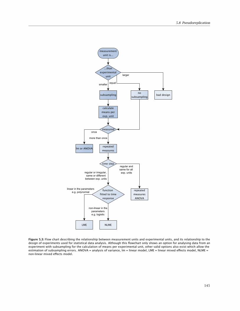
5.8 Pseudoreplication

Figure 5.3: Flow chart describing the relationship between measurement units and experimental units, and its relationship to thedesign of experiments used for statistical data analysis. Although this flowchart only shows an option for analysing data from anexperiment with subsampling for the calculation of means per experimental unit, other valid options also exist which allow theestimation of subsampling errors. ANOVA = analysis of variance, lm = linear model, LME = linear mixed effects model, NLME =non-linear mixed effects model.

145

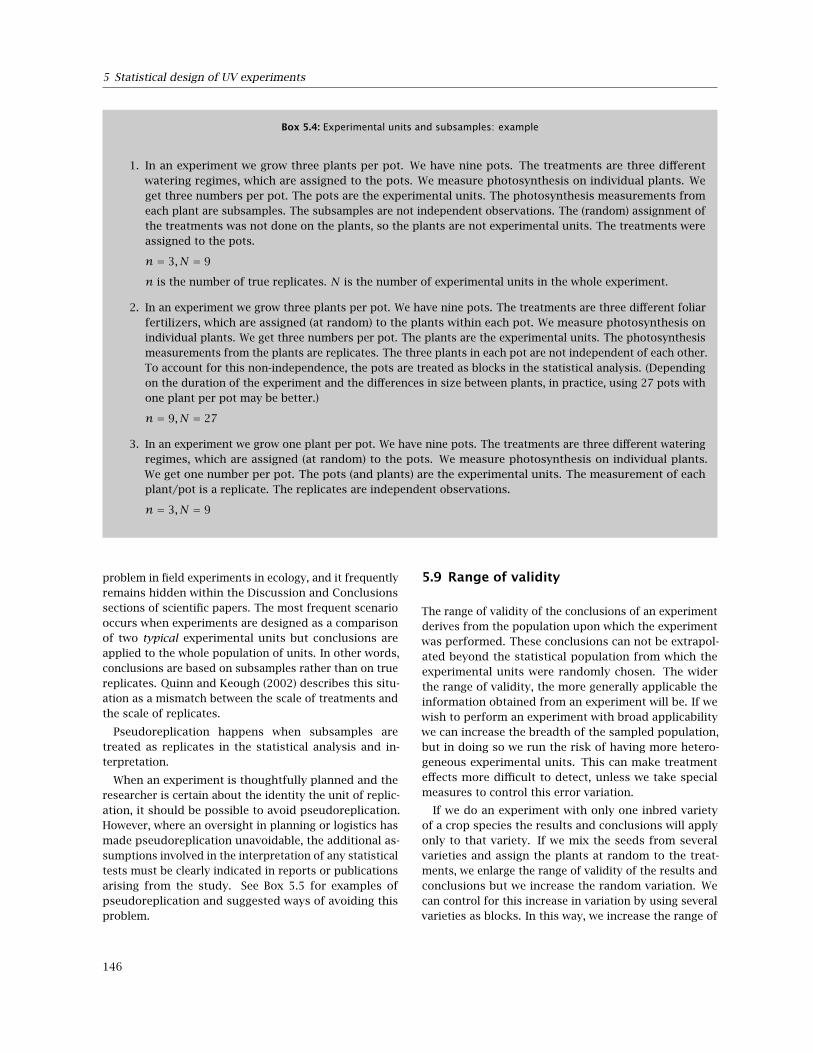
5 Statistical design of UV experiments

Box 5.4: Experimental units and subsamples: example

1. In an experiment we grow three plants per pot. We have nine pots. The treatments are three differentwatering regimes, which are assigned to the pots. We measure photosynthesis on individual plants. Weget three numbers per pot. The pots are the experimental units. The photosynthesis measurements fromeach plant are subsamples. The subsamples are not independent observations. The (random) assignment ofthe treatments was not done on the plants, so the plants are not experimental units. The treatments wereassigned to the pots.

n = 3, N = 9

n is the number of true replicates. N is the number of experimental units in the whole experiment.

2. In an experiment we grow three plants per pot. We have nine pots. The treatments are three different foliarfertilizers, which are assigned (at random) to the plants within each pot. We measure photosynthesis onindividual plants. We get three numbers per pot. The plants are the experimental units. The photosynthesismeasurements from the plants are replicates. The three plants in each pot are not independent of each other.To account for this non-independence, the pots are treated as blocks in the statistical analysis. (Dependingon the duration of the experiment and the differences in size between plants, in practice, using 27 pots withone plant per pot may be better.)

n = 9, N = 27

3. In an experiment we grow one plant per pot. We have nine pots. The treatments are three different wateringregimes, which are assigned (at random) to the pots. We measure photosynthesis on individual plants.We get one number per pot. The pots (and plants) are the experimental units. The measurement of eachplant/pot is a replicate. The replicates are independent observations.

n = 3, N = 9

problem in field experiments in ecology, and it frequentlyremains hidden within the Discussion and Conclusionssections of scientific papers. The most frequent scenariooccurs when experiments are designed as a comparisonof two typical experimental units but conclusions areapplied to the whole population of units. In other words,conclusions are based on subsamples rather than on truereplicates. Quinn and Keough (2002) describes this situ-ation as a mismatch between the scale of treatments andthe scale of replicates.

Pseudoreplication happens when subsamples aretreated as replicates in the statistical analysis and in-terpretation.

When an experiment is thoughtfully planned and theresearcher is certain about the identity the unit of replic-ation, it should be possible to avoid pseudoreplication.However, where an oversight in planning or logistics hasmade pseudoreplication unavoidable, the additional as-sumptions involved in the interpretation of any statisticaltests must be clearly indicated in reports or publicationsarising from the study. See Box 5.5 for examples ofpseudoreplication and suggested ways of avoiding thisproblem.

5.9 Range of validity

The range of validity of the conclusions of an experimentderives from the population upon which the experimentwas performed. These conclusions can not be extrapol-ated beyond the statistical population from which theexperimental units were randomly chosen. The widerthe range of validity, the more generally applicable theinformation obtained from an experiment will be. If wewish to perform an experiment with broad applicabilitywe can increase the breadth of the sampled population,but in doing so we run the risk of having more hetero-geneous experimental units. This can make treatmenteffects more difficult to detect, unless we take specialmeasures to control this error variation.

If we do an experiment with only one inbred varietyof a crop species the results and conclusions will applyonly to that variety. If we mix the seeds from severalvarieties and assign the plants at random to the treat-ments, we enlarge the range of validity of the results andconclusions but we increase the random variation. Wecan control for this increase in variation by using severalvarieties as blocks. In this way, we increase the range of

146

5.9 Range of validity

Box 5.5: Pseudoreplication: examples

Problem 1: We want to study the effect of UV radiation on the growth of plants. We have two rooms, one with onlynormal lamps supplying PAR and one with some UV lamps in addition to the normal lamps. We randomlyassign 20 plants to each room. We measure the height of the plants after one week. This experiment has20 subsamples per treatment, but only one replicate. (The UV treatments were assigned at random to therooms, not to the plants). It is not valid to treat the subsamples as replicates and try to draw conclusionsabout the effect of UV radiation, since we have only pseudoreplicates. In this case pseudoreplication addsthe implicit assumption that the only difference between the rooms was the UV irradiance. Our statisticaltest really only answers the question: did the plants grow differently in the two rooms?

Solution 1: Several remedies are needed to obtain a wider range of validity from this experiment. Replicates intime can be created by repeating the experiment several times swapping the UV lamps between rooms. Sucha situation is far from ideal because it is difficult to maintain plants and rooms in an equivalent state overtime, since factors such as time of year and deterioration of lamps and filters must be accounted for. Anadditional step towards overcoming this problem would be to make a pre-experimental trial trying to create’identical’ conditions in both growth rooms and checking whether this results in any difference in plantperformance.

Problem 2: We want to study the differences between high elevation and lowland meadow vegetation. We chooseone typical lowland meadow (LM) and one high elevation meadow (HM). We establish 5 plots, located atrandom, within each meadow. In each plot we mark ten 1 m2 sampling areas at random, and record thespecies composition within these areas.

Solution 2: It is not valid to try to answer the question ‘is species x more frequent in lowland meadows than inhighland meadows’ using the plots as replicates, since we have only pseudoreplication. The context of thequestion posed is critical in this instance. For this question we have, one true replicate (one meadow ofeach type), 5 subsamples (the plots) within each meadow, and 10 subsubsamples within each subsample. Ifthe experiment is performed as described, it can only answer the question: “Is species x more abundant inmeadow ‘LM’ than meadow ‘HM’?” If we want to draw conclusions about the two (statistical) populationsof meadows, we should sample at random from those populations. For example compare five differenthighland meadows to five lowland meadows.

Problem 3: We have three UV-B lamp frames. The radiation from the lamps in one frame is filtered with cellulosedi-acetate, in another frame the lamps are filtered with polyester, and in the third frame the lamps are notenergized. We chose at random three groups of 100 seedlings and put one group under each frame. This isan un-replicated experiment, we have one experimental unit (one lamp frame) per treatment. If we use theplants as replicates, we commit pseudoreplication. The plants are subsamples, not replicates.

Solution 3: Ideally we would try to obtain more lamp frames. If this was impossible, a replicated experimentcould be created by sub-dividing the area under each lamp frame into two separate parts, and allocating onehalf of each containing 50 seedlings to be filtered by cellulose di-acetate and the other half by polyester. Theunenergised lamp treatment would have to be omitted, but this compromise would enable three replicatesof the two treatments to be created. Each lamp frame would be a block.

Problem 4: We have nine UV-B lamp frames, three for each treatment. We put 100 plants under each frame asabove. We do the statistical analysis based on the measurements on each plant considering the plants asreplicates, we commit pseudoreplication. Our estimate of the error variance is wrong, as it does not reflectthe variation among frames with the same treatment, and degrees of freedom are hugely inflated.

Solution 4: Alternatively, we do the experiment exactly as in the item above, but we calculate means per frame forthe measured variable, and then use these means in the statistical analysis. In other words we analyse ourdata using the frames as replicates. We have a valid test of significance, because the error variance reflectsthe variation between equally treated experimental units (the lamp frames). Logistical constraints oftenrequire that a decision must be made about whether to measure more plants under fewer replicates, orfewer plants under more replicates. When such a compromise has to be made, it is nearly always preferableto have more experimental units and to measure fewer plants within each one, even at the expense of greaterallocation of time and resources to the maintenance of filters and lamp frames.

147

5 Statistical design of UV experiments

validity of the results and conclusions without increasingthe random variation.

The design of an experiment involves many comprom-ises concerning its range of validity, these relate to trade-offs between generality, precision, and realism, not tomention cost.

5.9.1 Factorial experiments

One way of increasing the range of validity of the resultsof a scientific study is to use a factorial design for anexperiment. For example, if we study the effects of UVradiation on well-watered plants only, then the conclu-sions of our study will be valid only for well-wateredplants. If we include a second factor in our design withthree levels, ‘drought’, ‘mild drought’ and ‘well watered’and include all the treatment combinations possible, e.g.based on the three levels of watering and three levels ofUV attenuation we have nine treatments and the rangeof validity is greatly expanded. In addition we can statist-ically test whether these two factors interact4. Factorialexperiments are a very powerful and useful design butif too many factors and levels are included their inter-pretation may become difficult. Factorial experimentswith many factors and/or levels result in a statistical ana-lysis based on many different contrasts5. In this case, weshould remember that in most analyzes we wish to ob-tain P -values per contrast, rather than per experiment. Ifwe want to keep the experiment-wise risk level constant,we should use a tight contrast-wise risk level, or adjustthe P -values.

The flowchart in Figure 5.4 describes the relationshipsbetween the structure of treatments and data analysis.

5.10 When not to make multiplecomparisons

In the biological literature, multiple comparison proced-ures such as Tukey’s HSD are frequently used in situ-ations where other tests would be more effective andeasier to interpret. In some other cases multiple compar-isons are used in situations in which they give misleadingresults. We will discuss the two most common cases ofmisuse of these tests.

5.10.1 Dose response curves

If we have several levels of the same treatment, for ex-ample several different irradiances of UV, the most power-

ful (capable of reliably detecting effects) test is to fit aregression (either linear or non-linear) of the responseon the “dose”. From such an analysis we get informationon the relationship between dose and response, whetherit is increasing or decreasing, linear or curvilinear, evenits shape can be inferred. In many cases we can alsocalculate a confidence band around the fitted function.This is all useful and interpretable information.

If instead we calculate for example HSD or LSD andcompare the responses to all possible pairs of doses, wediscard the information about the ordering of the doses,and we can get results that do not address our researchhypothesis, for example, concluding that all pairs of ad-jacent doses do not differ significantly while the extremedoses do differ significantly. In this type of experimentswe are really interested in the slope and shape of a doseresponse curve.

Multiple comparisons should be carried out only whenthere is no ordering in the levels of a treatment of factor.A regression or ANCOVA model should be used instead,if a reasonable model can be fitted.

5.10.2 Factorial experiments

Factorial experiments are very useful and as discussedabove allow extending the range of validity of our con-clusions. However, the main advantage of factorial ex-periments is that the significance of interactions can betested. The most important part of the statistical analysisof a factorial experiment is an ANOVA with a model in-cluding main effects and interactions. Only after this test,one can in addition, test the differences among differentpairs of treatments. This a posteriori test provides littleextra information and should be done only if the inter-action term is statistically significant. Otherwise, if thelevels of a factor are discrete and unordered, and its maineffect is significant in ANOVA, a multiple comparison testcan be used to compare the levels of a factor (but not theindividual combinations of levels of the different factors).

5.11 Presenting data in figures

When using hierarchical designs such as split-plots, theexperimental errors relevant to comparisons betweenlevels of the different factors will be different. In suchdesigns, it is especially important to indicate which errorterm the error bars in figures show. In all cases, the figureand table legends should state which statistics are depic-ted by the error bars, and also the number of replicates

4The main difference between a design with blocks and a factorial design, is that in the first case it is assumed that there is no interaction betweentreatments and blocks, and the interaction term is used as an estimator of the error variance while in a factorial design we estimate the errorvariance based on equally treated units and we do not need to assume the lack of interaction effect.

5In ANOVA, a contrast is a combination of factor level means (two or more) based on multipliers that add to zero. Each contrast defines one ofmany possible tests of significance.

148

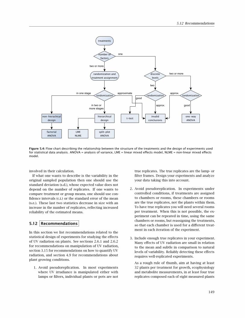
5.12 Recommendations

Figure 5.4: Flow chart describing the relationship between the structure of the treatments and the design of experiments usedfor statistical data analysis. ANOVA = analysis of variance, LME = linear mixed effects model, NLME = non-linear mixed effectsmodel.

involved in their calculation.If what one wants to describe is the variability in the

original sampled population then one should use thestandard deviation (s.d.), whose expected value does notdepend on the number of replicates. If one wants tocompare treatment or group means, one should use con-fidence intervals (c.i.) or the standard error of the mean(s.e.). These last two statistics decrease in size with anincrease in the number of replicates, reflecting increasedreliability of the estimated means.

5.12 Recommendations

In this section we list recommendations related to thestatistical design of experiments for studying the effectsof UV radiation on plants. See sections 2.6.1 and 2.6.2for recommendations on manipulation of UV radiation,section 3.15 for recommendations on how to quantify UVradiation, and section 4.9 for recommendations aboutplant growing conditions.

1. Avoid pseudoreplication. In most experimentswhere UV irradiance is manipulated either withlamps or filters, individual plants or pots are not

true replicates. The true replicates are the lamp- orfilter frames. Design your experiments and analyzeyour data taking this into account.

2. Avoid pseudoreplication. In experiments undercontrolled conditions, if treatments are assignedto chambers or rooms, these chambers or roomsare the true replicates, not the plants within them.To have true replicates you will need several roomsper treatment. When this is not possible, the ex-periment can be repeated in time, using the samechambers or rooms, but reassigning the treatments,so that each chamber is used for a different treat-ment in each iteration of the experiment.

3. Include enough true replicates in your experiment.Many effects of UV radiation are small in relationto the mean and subtle in comparison to naturallevels of variability. Reliably detecting these effectsrequires well-replicated experiments.

As a rough rule of thumb, aim at having at least32 plants per treatment for growth, ecophysiologyand metabolite measurements, in at least four truereplicates composed each of eight measured plants

149

5 Statistical design of UV experiments

in controlled environment and greenhouse studies.When making gas-exchange readings, it is usuallyimpractical to measure from more than four to sixplants in each of the four true replicates. If you aimto make an ecologically-orientated outdoor studyit would be advisable to have at least five true rep-licates. In addition to issues of replication, in mostcases you will need to have unmeasured borderplants surrounding your experimental plants so asto avoid edge effects. Alternatively the positions ofplants can be rotated every few days.

4. Preferably use a design with blocks to control allknown or expected sources of error (or backgroundvariation) that would otherwise confound the treat-ment effects. Examples of such sources of variationare different benches in a greenhouse, or measure-ments done by different observers. If you suspectthat a known source of error may interact with yourUV treatment, you may decide to consider it as acovariate in your model.

5. Within the blocks, use randomization to neutral-ize the effects of other error sources. Randomiza-tion is of fundamental importance and should bedone properly: i.e. a device that generates a trulyrandom assignment of treatments to experimentalunits should be employed. Such devices can be assimple as a coin, or die, or can be a table of randomnumbers in a book, or (pseudo-) random numbersgenerated by a computer or a pocket calculator.

6. When designing an experiment use power analysisto determine the number of replicates needed, un-less you have a long experience of performing sim-ilar experiments, and a good existing understand-

ing of the amount of variability you expect to findin your results.

7. If your experiment yields a non-significant differ-ence, use a posteriori power analysis to demon-strate, if possible, that biologically important dif-ferences would have been detected had they existed.However, if power analysis reveals that your exper-iment was unable to detect biologically importantdifferences, you should repeat the experiment withmore replicates or an improved design.

5.13 Further reading

A reliable on-line resource is the Statistics Stack Exchange(http://stats.stackexchange.com/).

There are many text books on statistics, but most in-troductory statistical texts do not discuss the type ofhierarchical models usually needed for UV experiments.We recommend the classic book ‘Planning of Experiments’by Cox (1958) as a good introduction to the principlesbehind the design of experiments. ‘Experimental Designand Data Analysis for Biologists’ by Quinn and Keough(2002) describes both experimental design and analysisof data at an intermediate level. The books ‘EcologicalModels and Data in R’ (Bolker, 2008) and ‘Mixed effectsmodels and extensions in ecology with R’ (Zuur, Ieno,Walker et al., 2009) give advanced up-to-date accountsof statistical methods, and approaches, including a dis-cussion of hypothesis testing and model fitting. While‘A Beginner’s Guide to R’ (Zuur, Ieno and Meesters, 2009)and ‘Introductory Statistics with R’ (Dalgaard, 2002) aregentle introductions to data analysis with R.

150

Bibliography

Albert, A. and P. Gege (2006). ‘Inversion of irradiance andremote sensing reflectance in shallow water between400 and 800 nm for calculations of water and bottomproperties’. In: Applied Optics 45, pp. 2331–2343. doi:10.1364/AO.45.002331 (cit. on p. 20).

Albert, A. and C. D. Mobley (2003). ‘An analytical modelfor subsurface irradiance and remote sensing reflect-ance in deep and shallow case-2 waters’. In: OpticsExpress 11.22, pp. 2873–2890. url: http://www.opticsexpress.org/abstract.cfm?URI=OPEX-11-22-2873 (cit. on pp. 15, 20).

Allen, L. H., H. W. Gausman and W. A. Allen (1975).‘Solar Ultraviolet Radiation in Terrestrial Plant Com-munities’. In: Journal of Environmental Quality4.3, pp. 285–294. doi: 10 . 2134 / jeq1975 .00472425000400030001x (cit. on p. 11).

Anderson, J., W. Chow and D. Goodchild (1988).‘Thylakoid Membrane Organisation in Sun/Shade Accli-mation’. In: Functional Plant Biology 15, pp. 11–26. doi:10.1071/PP9880011 (cit. on p. 124).

Aphalo, P. J. (2003). ‘Do current levels of UV-B radiationaffect vegetation? The importance of long-term experi-ments’. In: New Phytologist 160. Invited commentary,pp. 273–276. doi: 10.1046/j.1469-8137.2003.00905.x (cit. on p. 2).

Aphalo, P. J., R. Tegelberg and R. Julkunen-Tiitto (1999).‘The modulated UV-B irradiation system at the Uni-versity of Joensuu’. In: Biotronics 28, pp. 109–120.url: http : / / ci . nii . ac . jp / naid /110006175827/en (cit. on pp. 39, 48–50).

Arends, G., R. K. A. M. Mallant, E. van Wensveen and J. M.Gouman (1988). A fog chamber for the study of chem-ical reactions. Tech. rep. Report - ECN - 210. Petten,Netherlands (cit. on p. 126).

Arfsten, D. P., D. J. Schaeffer and D. C. Mulveny (1996).‘The effects of near ultraviolet radiation on the toxiceffects of polycyclic aromatic hydrocarbons in anim-als and plants: A review’. In: Ecotoxicology and Envir-onment Safety 33, pp. 1–24. doi: 10.1006/eesa.1996.0001 (cit. on p. 19).

Arts, M. T., R. D. Robarts, F. Kasai, M. J. Waiser, V. P.Tumber, A. J. Plante, H. Rai and H. J. de Lange (2000).‘The attenuation of ultraviolet radiation in high dis-solved organic carbon waters of wetlands and lakes onthe northern Great Plains’. In: Limnology and Oceano-

graphy 45, pp. 292–299. url: http://www.jstor.org/stable/2670483 (cit. on p. 18).

Austin, A. T. and C. L. Ballaré (2010). ‘Dual role of ligninin plant litter decomposition in terrestrial ecosystems’.In: Procceedings of the National Academy of Sciences ofthe U.S.A 107, pp. 4618–4622. doi: 10.1073/pnas.0909396107 (cit. on p. 2).

Bakker, J. C., G. P. A. Bot, H. Challa and N. J. Vand de Braak,eds. (1995). Greenhouse climate control: An integratedapproach. Wageningen, The Netherlands: WageningenAcademic Publishers. 279 pp. isbn: 978-90-74134-17-0.doi: 10.3920/978-90-8686-501-7 (cit. onp. 138).

Ballaré, C. L., M. M. Caldwell, S. D. Flint, S. A. Robinson andJ. F. Bornman (2011). ‘Effects of solar ultraviolet radi-ation on terrestrial ecosystems. Patterns, mechanisms,and interactions with climate change’. In: Photochem-ical and Photobiological Sciences 10 (2), pp. 226–241.doi: 10.1039/C0PP90035D (cit. on p. 1).

Barnes, P. W., S. D. Flint, J. R. Slusser, W. Gao and R. J.Ryel (2008). ‘Diurnal changes in epidermal UV trans-mittance of plants in naturally high UV environments’.In: Physiologia Plantarum 133, pp. 363–372. doi: 10.1111/j.1399-3054.2008.01084.x (cit. onp. 21).

Bazzaz, F. A. and R. W. Carlson (1982). ‘Photosyntheticacclimation to variability in the light environment ofearly and late successional plants’. In: Oecologia 54,pp. 313–316. doi: 10.1007/BF00379999 (cit. onp. 124).

Belzile, C., S. Demers, G. A. Ferreyra, I. Schloss, C. Nozais,K. Lacoste, B. Mostajir, S. Roy, M. Gosselin, E. Pelletieret al. (2006). ‘UV effects on marine planktonic foodwebs: A synthesis of results from mesocosm studies’.In: Photochemistry and Photobiology 82, pp. 850–856.doi: 10.1562/2005-09-27-RA-699 (cit. onp. 136).

Belzile, C., S. Demers, D. R. S. Lean, B. Mostajir, S.Roy, S. de Mora, D. Bird, M. Gosselin, J. P. Chanutand M. Levasseur (1998). ‘An experimental tool tostudy the effects of ultraviolet radiation on plank-tonic communities: A mesocosm approach’. In: Environ-mental Technology 19, pp. 667–682. doi: 10.1080/09593331908616723 (cit. on p. 136).

151

Bibliography

Bentham (1997). A Guide to Spectroradiometry: Instru-ments & Applications for the Ultraviolet. Tech. rep. Read-ing, U.K.: Bentham Instruments Ltd (cit. on p. 110).

Bérces, A., A. Fekete, S. Gáspár, P. Gróf, P. Rettberg, G.Horneck and G. Rontó (1999). ‘Biological UV dosimet-ers in the assessment of the biological hazard fromenvironmental radiation’. In: Journal of Photochemistryand Photobiology, B 53.1-3, pp. 36–43. doi: 10.1016/S1011-1344(99)00123-2 (cit. on p. 78).

Berger, D. S. (1976). ‘The sunburning ultraviolet meter:design and performance’. In: Photochemistry and Pho-tobiology 24, pp. 587–593. doi: 10.1111/j.1751-1097.1976.tb06877.x (cit. on p. 80).

Beytes, C., ed. (2003). Ball Red Book: Greenhouses andequipment. 17th ed. Batavia, IL, USA: Ball Publishing.272 pp. isbn: 1883052343 (cit. on p. 138).

Bickford, E. D. and S. Dunn (1972). Lighting for plantgrowth. Ohio, USA: Kent State University Press. x + 221.isbn: 0873381165 (cit. on p. 48).

Bilger, W., T. Johnsen and U. Schreiber (2001). ‘UV-excitedchlorophyll fluorescence as a tool for the assessmentof UV-protection by epidermins of plants’. In: Journalof Experimental Botany 52, pp. 2007–2014. doi: 10.1093/jexbot/52.363.2007 (cit. on pp. 21, 23).

Bilger, W., M. Veit, L. Schreiber and U. Schreiber (1997).‘Measurement of leaf epidermal transmittance of UVradiation by chlorophyll fluorescence’. In: PhysiologiaPlantarum 101.4, pp. 754–763. doi: 10.1111/j.1399-3054.1997.tb01060.x (cit. on p. 21).

Bird, R. E. and C. Riordan (1986). ‘Simple solar spectralmodel for direct and diffuse irradiance on horizontaland tilted planes at the Earth’s surface for cloudlessatmospheres’. English. In: Journal of Climate and Ap-plied Meteorology 25.1, pp. 87–97. issn: 0733-3021. doi:10.1175/1520- 0450(1986)025%3C0087:SSSMFD%3E2.0.CO;2 (cit. on p. 97).

Bischof, K., I. Gómez, M. Molis, D. Hanelt, U. Karsten, U.Lüder, M. Y. Roleda, K. Zacher and C. Wiencke (2006).‘Ultraviolet radiation shapes seaweed communities’. In:Reviews in Evironmental Science and Biotechnology 51,pp. 141–166. doi: 10.1007/s11157-006-0002-3 (cit. on p. 131).

Björn, L. O. (1995). ‘Estimation of fluence rate from irradi-ance measurements with a cosine-corrected sensor’. In:Journal of Photochemistry and Photobiology B Biology29, pp. 179–183. doi: 10.1016/1011-1344(95)07135-O (cit. on p. 74).

Björn, L. O., ed. (2007). Photobiology: The Science of Lifeand Light. 2nd ed. Springer. 684 pp. isbn: 0387726543(cit. on pp. 2, 27, 76).

Björn, L. O. and T. M. Murphy (1985). ‘Computer calcula-tion of solar ultraviolet radiation at ground level’. In:

Physiologie Végétale 23, pp. 555–561 (cit. on pp. 97,98).

Björn, L. O. and A. H. Teramura (1993). ‘Simulation ofdaylight ultraviolet radiation and effects of ozone de-pletion’. In: Environmental UV Photobiology. Ed. by A. R.Young, L. O. Björn, J. Moan and W. Nultsch. New York:Plenum Press, pp. 41–71. isbn: 0-306-44443-7 (cit. onpp. 38, 40, 41, 67, 111).

Björn, L. O. and T. C. Vogelmann (1996). ‘Quantifyinglight and ultraviolet radiation in plant biology’. In: Pho-tochemistry and Photobiology 64, pp. 403–406. doi:10.1111/j.1751-1097.1996.tb03084.x(cit. on pp. 75, 76).

Bloom, A. A., J. Lee-Taylor, S. Madronich, D. J. Messen-ger, P. I. Palmer, D. S. Reay and A. R. McLeod (2010).‘Global methane emission estimates from ultravioletirradiation of terrestrial plant foliage’. In: New Phyto-logist 187.2, pp. 417–425. doi: 10.1111/j.1469-8137.2010.03259.x (cit. on p. 2).

Bolker, B. M. (2008). Ecological Models and Data in R. Prin-ceton University Press. 408 pp. isbn: 0691125228 (cit.on p. 150).

Booker, F. L., E. L. Fiscus, R. B. Philbeck, A. S. Heagle,J. E. Miller and W. W. Heck (1992). ‘A supplementalultraviolet-B radiation system for open-top chambers’.In: Journal of Environmental Quality 21, pp. 56–61 (cit.on p. 127).

Bornman, J. F. and T. C. Vogelmann (1988). ‘Penetrationby blue and UV radiation measured by fiber optics inspruce and fir needles’. In: Physiologia Plantarum 72.4,pp. 699–705. doi: 10.1111/j.1399-3054.1988.tb06368.x (cit. on p. 21).

Bowman, W. D. and J. N. Demas (1976). ‘Ferrioxalate ac-tinometry - Warning on its correct use’. In: Journal ofPhysical Chemistry 80.21, pp. 2434–2435. issn: 0022-3654. doi: 10.1021/j100562a025 (cit. on p. 77).

Braslavsky, S. E. (2007). ‘Glossary of terms used in Pho-tochemistry 3(rd) Edition (IUPAC Recommendations2006)’. In: Pure and Applied Chemistry 79.3, pp. 293–465. doi: 10.1351/pac200779030293 (cit. onp. 71).

Bricaud, A., M. Babin, A. Morel and H. Claustre (1995).‘Variability in the chlorophyll-specific absorption coeffi-cients of natural phytoplankton: analysis and paramet-erization’. In: Journal of Geophysical Research 100.C7,pp. 13321–13332 (cit. on p. 17).

Bricaud, A., A. Morel and L. Prieur (1981). ‘Absorption bydissolved organic matter of the sea (yellow substance)in the UV and visible domains’. In: Limnology andOceanography 26.1, pp. 43–53. url: http://www.jstor.org/stable/2835805 (cit. on p. 16).

Brown, M. J., G. G. Parker and N. E. Posner (1994). ‘Asurvey of ultraviolet-B radiation in forests’. In: Journal

152

Bibliography

of Ecology 82.4, pp. 843–854. url: http://www.jstor.org/stable/2261448 (cit. on pp. 11,14).

Buiteveld, H., J. H. M. Hakvoort and M. Donze (1994). ‘Theoptical properties of pure water’. In: Proceedings of SPIE“Ocean Optics XII”. Vol. 2258. International Society forOptical Engineering, pp. 174–183 (cit. on p. 16).

Cabello-Pasini, A., E. Aguirre-von-Wobeser and F. L.Figueroa (2000). ‘Photoinhibition of photosynthesis inMacrocystis pyrifera (Phaeophyceae), Chondrus crispus(Rhodophyceae) and Ulva lactuca (Chlorophyceae) inoutdoor culture systems’. In: Journal of Photochem-istry and Photobiology B: Biology 57, pp. 169–178. doi:10.1016/S1011-1344(00)00095-6 (cit. onp. 134).

Caldwell, M. M. (1971). ‘Solar UV irradiation and thegrowth and development of higher plants’. In: Pho-tophysiology. Ed. by A. C. Giese. Vol. 6. New York: Aca-demic Press, pp. 131–177. isbn: 012282606X (cit. onpp. xxiii, 1, 25, 105, 111).

Caldwell, M. M. and S. D. Flint (1994a). ‘Lighting consid-erations in controlled environments for nonphotosyn-thetic plant responses to blue and ultraviolet radiation’.In: Proceedings of the International Lighting in Con-trolled Environments Workshop. Vol. NASA-CP-95-3309,pp. 113–124 (cit. on p. 50).

– (1994b). ‘Stratospheric ozone reduction, solar UV-B ra-diation and terrestrial ecosystems’. In: Climatic Change28.4, pp. 375–394. doi: 10.1007/BF01104080 (cit.on p. 1).

Caldwell, M. M. and S. D. Flint (2006). ‘Use and Evalu-ation of Biological Spectral UV Weighting Functionsfor the Ozone Reduction Issue’. In: Environmental UVRadiation: Impact on Ecosystems and Human Healthand Predictive Models. Ed. by F. Ghetti, G. Checcucciand J. F. Bornman. Vol. 57. NATO Science Series. Pro-ceedings of the NATO Advanced Study Institute onEnvironmental UV Radiation: Impact on Ecosystemsand Human Health and Predictive Models Pisa, ItalyJune 2001. Dordrecht: Springer, pp. 71–84. isbn: 978-1-4020-3695-8. doi: 10.1007/1-4020-3697-3(cit. on p. 102).

Caldwell, M. M., S. D. Flint and P. S. Searles (1994).‘Spectral balance and UV-B sensitivity of soybean: Afield experiment’. In: Plant, Cell and Environment 17.3,pp. 267–276. doi: 10.1111/j.1365-3040.1994.tb00292.x (cit. on p. 1).

Caldwell, M. M., W. G. Gold, G. Harris and C. W. Ashurst(1983). ‘A modulated lamp system for solar UV-B (280-320 nm) supplementation studies in the field’. In: Pho-tochemistry and Photobiology 37, pp. 479–485. doi:10.1111/j.1751-1097.1983.tb04503.x(cit. on pp. 48, 136).

Caldwell, M. M., A. H. Teramura and M. Tevini (1989). ‘TheChanging Solar Ultraviolet Climate and the EcologicalConsequences for Higher Plants’. In: Trends in Ecology& Evolution 4.12, pp. 363–367. doi: 10.1016/0169-5347(89)90100-6 (cit. on p. 1).

Campbell, G. S. and J. M. Norman (1998). An Introduc-tion to Environmental Biophysics. 2nd ed. New York:Springer. 286 pp. isbn: 0-387-94937-2 (cit. on p. 15).

Cen, Y.-P. and J. F. Bornman (1993). ‘The effect of expos-ure to enhanced UV-B radiation on the penetration ofmonochromatic and polychromatic UV-B radiation inleaves of Brassica napus’. In: Physiologia Plantarum87.3, pp. 249–255. doi: 10.1111/j.1399-3054.1993.tb01727.x (cit. on p. 21).

Christie, J. M. (2007). ‘Phototropin Blue-Light Receptors’.In: Annual Review of Plant Biology 58, pp. 21–45. doi:10.1146/annurev.arplant.58.032806.103951 (cit. on p. 1).

Christie, J. M., A. S. Arvai, K. J. Baxter, M. Heilmann,A. J. Pratt, A. O’Hara, S. M. Kelly, M. Hothorn, B. O.Smith, K. Hitomi et al. (2012). ‘Plant UVR8 Photore-ceptor Senses UV-B by Tryptophan-Mediated Disrup-tion of Cross-Dimer Salt Bridges’. In: Science. doi: 10.1126/science.1218091 (cit. on p. 1).

Cochran, W. G. (1957). ‘Analysis of covariance its natureand uses’. In: Biometrics 13, pp. 261–281. url: http://www.jstor.org/stable/2527916 (cit. onp. 143).

Cohen, J. (1977). Statistical Power Analysis for the Beha-vioral Sciences. Revised edition. New York: AcademicPress. 474 pp. (cit. on p. 139).

Coleman, A., R. Sarkany and S. Walker (2008). ‘Clinicalultraviolet dosimetry with a CCD monochromator ar-ray spectroradiometer’. In: Physics in Medicine and Bio-logy 53.18, pp. 5239–5255. doi: 10.1088/0031-9155/53/18/026 (cit. on p. 94).

Coohill, T. P. (Oct. 1992). ‘Action spectroscopy and strato-spheric ozone depletion’. In: UV-B monitoring workshop:a review of the science and status of measuring andmonitoring programs. Science and Policy Associaties,Washington D.C., pp. C89–C112 (cit. on p. 24).

Cooley, N. M., H. M. F. Truscott, M. G. Holmes and T. H.Attridge (2000). ‘Outdoor ultraviolet polychromatic ac-tion spectra for growth responses of Bellis perennisand Cynosurus cristatus’. In: Journal of Photochemistryand Photobiology B: Biology 59.1-3, pp. 64–71. doi:10.1016/S1011-1344(00)00141-X (cit. onp. 27).

Cox, D. R. (1958). Planning of Experiments. New York:John Wiley & Sons. 308 pp. (cit. on pp. 142, 150).

Cox, D. R. and N. Reid (2000). The Theory of the Design ofExperiments. 1st ed. Chapman and Hall/CRC. 314 pp.isbn: 158488195X (cit. on p. 140).

153

Bibliography

Crawley, M. J. (2005). Statistics: An Introduction using R.Wiley. 342 pp. isbn: 0470022981 (cit. on p. 116).

– (2007). The R Book. John Wiley and Sons Ltd. 950 pp.isbn: 0470510242 (cit. on p. 116).

Cullen, J. J. and P. J. Neale (1997). ‘Biological weight-ing functions for describing the effects of ultravioletradiation on aquatic systems’. In: The effects of ozonedepletion on aquatic ecosystems. Ed. by D.-P. Häder. Aca-demic Press. Chap. 6, pp. 97–118. isbn: 0123991730(cit. on pp. 23, 26).

Dalgaard, P. (2002). Introductory Statistics with R. Statist-ics and Computing. New York: Springer. xv + 267. isbn:0 387 95475 9 (cit. on pp. 116, 150).

D’Antoni, H. L., L. J. Rothschild, C. Schultz, S. Burgessand J. W. Skiles (2007). ‘Extreme environments inthe forests of Ushuaia, Argentina’. In: Geophysical Re-search Letters 34.22. issn: 0094-8276. doi: 10.1029/2007GL031096 (cit. on p. 92).

D’Antoni, H. L., L. J. Rothschild and J. W. Skiles (2008).‘Reply to comment by Stephan D. Flint et al. on “Ex-treme environments in the forests of Ushuaia, Argen-tina”’. In: Geophysical Research Letters 35.13. issn:0094-8276. doi: 10.1029/2008GL033836 (cit. onp. 92).

Deckmyn, G., E. Cayenberghs and R. Ceulemans (2001).‘UV-B and PAR in single and mixed canopies grownunder different UV-B exclusions in the field’. In:Plant Ecology 154, 125–133. doi: 10 . 1023 / A :1012920716047 (cit. on p. 11).

Dekker, A. G. (1993). ‘Detection of optical water qualityparameters for eutrophic waters by high resolutionremote sensing’. PhD thesis. Vrije Universiteit Amster-dam (cit. on pp. 15, 17, 18, 20).

de la Rosa, T. M., R. Julkunen-Tiitto, T. Lehto and P. J.Aphalo (2001). ‘Secondary metabolites and nutrientconcentrations in silver birch seedlings under fivelevels of daily UV-B exposure and two relative nutrientaddition rates’. In: New Phytologist 150, pp. 121–131.doi: 10.1046/j.1469-8137.2001.00079.x(cit. on p. 60).

DeLucia, E. H., T. A. Day and T. C. Vogelman (1992).‘Ultraviolet-B and visible light penetration into needlesof two species of subalpine conifers during foliardevelopment’. In: Plant, Cell and Environment 15.8,pp. 921–929. doi: 10.1111/j.1365-3040.1992.tb01024.x (cit. on p. 21).

Demas, J. N., W. D. Bowman, E. F. Zalewski and R. A.Velapoldi (1981). ‘Determination of the quantum yieldof the ferrioxalate actinometer with electrically cal-ibrated radiometers’. In: Journal of Physical Chem-istry 85.19, pp. 2766–2771. issn: 0022-3654. doi: 10.1021/j150619a015 (cit. on p. 78).

den Outer, P., H. Slaper, J. Kaurola, A. Lindfors, A.Kazantzidis, A. Bais, U. Feister, J. Junk, M. Janouch andW. Josefsson (2010). ‘Reconstructing of erythemal ultra-violet radiation levels in Europe for the past 4 decades’.In: Journal of Geophysical Research (Atmospheres)115.D14, D10102. doi: 10.1029/2009JD012827(cit. on pp. 97, 98).

Díaz, S. B., J. E. Frederick, T. Lucas, C. R. Booth and I. Smol-skaia (1996). ‘Solar ultraviolet irradiance at Tierra delFuego: Comparison of measurements and calculationsover a full annual cycle’. In: Geophysical Research Let-ters 23.4, pp. 355 –358. doi: 10.1029/96GL00253(cit. on p. 10).

Díaz, S. B., J. H. Morrow and C. R. Booth (2000). ‘UV phys-ics and optics’. In: The Effects of UV Radiation in theMarine Environment. Ed. by S. de Mora, S. Demers andM. Vernet. Cambridge University Press, pp. 35–71 (cit.on p. 95).

Díaz, S., C. Camilión, J. Escobar, G. Deferrari, S. Roy, K.Lacoste, S. Demers, C. Belzile, G. Ferreyra, S. Gianesellaet al. (2006). ‘Simulation of ozone depletion using am-bient irradiance supplemented with UV lamps.’ In: Pho-tochemistry and Photobiology 82.4, pp. 857–864. doi:10.1562/2005-09-28-RA-700 (cit. on pp. 48,136).

Díaz, S., C. Camilión, K. Lacoste, J. Escobar, S. Demers,S. Gianesella and S. Roy (2003). ‘Simulation of increas-ing UV radiation as a consequence of ozone depletion’.In: Proceedings SPIE’s 48th annual meeting: Ultravi-olet ground- and spacebased measurements, modelsand effects III. Ed. by J. Slusser, J. Herman and W. Gao.SPIE: The International Sociaty for Optical Engineering,pp. 216 –227 (cit. on p. 136).

Diffey, B. L. (1987). ‘A comparison of dosimeters usedfor solar ultraviolet radiometry’. In: Photochem Photo-biol 46, pp. 55–60. doi: 10.1111/j.1751-1097.1987.tb04735.x (cit. on p. 79).

– (1989). Radiation Measurement in Photobiology. Lon-don: Academic Press. 230 pp. isbn: 0122158407 (cit.on p. 111).

Dixon, J. M., M. Taniguchi and J. S. Lindsey (2005). ‘Pho-tochemCAD 2: a refined program with accompanyingspectral data bases for photochemical calculations’. In:Photochemistry and Photobiology 81.1, pp. 212–213.doi: 10.1111/j.1751-1097.2005.tb01544.x (cit. on p. 17).

Döhring, T., M. Köfferlein, S. Thiel and H. K. Seidlitz(1996). ‘Spectral shaping of artificial UV-B irradiationfor vegetation stress research’. In: Journal of PlantPhysiology 148, pp. 115–119. doi: 10.1016/S0176-1617(96)80302-6 (cit. on pp. 50, 54).

Donahue, W. F., D. W. Schindler, S. J. Page and M. P. Stain-ton (1998). ‘Acid-induced changes in DOC quality in

154

Bibliography

an experimental whole-lake manipulation’. In: Environ-mental Science and Technology 32, pp. 2954–2960. doi:10.1021/es980306u (cit. on p. 18).

Du, H., R.-. C. A. Fuh, J. Li, L. A. Corkan and J. S. Lindsey(1998). ‘PhotochemCAD: a computer-aided design andresearch tool in photochemistry’. In: Photochemistryand Photobiology 68.2, pp. 141–142. doi: 10.1111/j.1751-1097.1998.tb02480.x (cit. on p. 17).

Dunne, R. P. (1999). ‘Polysulphone film as an underwa-ter dosimeter for solar ultraviolet-B radiation in trop-ical latitudes’. In: Marine Ecology Progress Series 189,pp. 53–63. doi: 10.3354/meps189053 (cit. onp. 78).

Eichler, H.-. J., A. Fleischner, J. Kross, M. Krystek, H. Lang,H. Niedrig, H. Rauch, G. Schmahl, H. Schoenebeck, E.Sedlmayr et al. (1993). Bergmann, Schaefer: Lehrbuchder Experimentalphysik Band 3: Optik. Ed. by H. Niedrig.Verlag Walter de Gruyter Berlin/New York (cit. on p. 3).

Einstein, A. (1910). ‘Theorie der Opaleszenz von homo-genen Flüssigkeiten und Flüssigkeitsgemischen in derNähe des kritischen Zustandes’. In: Annalen der PhysikIV. Folge 33.16, pp. 1275–1298 (cit. on p. 16).

Eisinger, W., T. E. Swartz, R. A. Bogomolni and L. Taiz(2000). ‘The ultraviolet action spectrum for stomatalopening in broad bean’. In: Plant Physiology 122, pp. 99–105. doi: http://dx.doi.org/10.1104/pp.122.1.99 (cit. on p. 131).

Engelsen, O. and A. Kylling (2005). ‘Fast simulation toolfor ultraviolet radiation at the earth’s surface’. In: Op-tical Engineering 44.4. doi: 10.1117/1.1885472(cit. on pp. 97, 98).

Fernández, E., J. M. Figuera and A. Tobar (1979). ‘Useof the potassium ferrioxalate actinometer below 254-nm’. In: Journal of Photochemistry 11.1, pp. 69–71.issn: 0047-2670. doi: 10.1016/0047-2670(79)85008-X (cit. on pp. 77, 78).

Figueroa, F. L., A. Bueno, N. Korbee, R. Santos, L. Mata andA. Schuenhoff (2008). ‘Accumulation of mycosporine-like amino acids in Asparagopsis armata grown intanks with fishpond effluents of gilthead sea bream,Asparus aurata’. In: Journal of the World AquacultureSociety 39, pp. 692 –699. doi: 10.1111/j.1749-7345.2008.00199.x (cit. on p. 134).

Figueroa, F. L., S. Salles, J. Aguilera, C. Jiménez, J. Mer-cado, B. Viñegla, A. Flores-Moya and M. Altamirano(1997). ‘Effects of solar radiation on photoinhibitionand pigmentation in the red alga Porphyra leucosticta’.In: Marine Ecology Progress Series 151, pp. 81–90. doi:10.3354/meps151081 (cit. on p. 62).

Figueroa, F. L., R. Santos, R. Conde-Álvarez, L. Mata, J. L.Gómez-Pinchetti, J. Matos, P. Huovinen, A. Schüehoffand J. Silva (2006). ‘The use of chlorophyll fluorescencefor monitoring photosynthetic conditions of two tank

cultivated red macroalgae using fishpond effluents’.In: Botanica Marina 49, pp. 275–282. doi: 10.1515/BOT.2006.035 (cit. on p. 134).

Fioletov, V. E., M. G. Kimlin, N. Krotkov, L. J. B. McArthur,J. B. Kerr, D. I. Wardle, J. R. Herman, R. Meltzer, T. W.Mathews and J. Kaurola (2004). ‘UV index climatologyover the United States and Canada from ground-basedand satellite estimates’. In: Journal of Geophysical Re-search - Atmospheres 109.D22. issn: 0148-0227. doi:10.1029/2004JD004820 (cit. on p. 97).

Fioletov, V., L. McArthur, J. Kerr and D. Wardle (2001).‘Long-term variations of UV-B irradiance over Canadaestimated from Brewer observations and derived fromozone and pyranometer measurements’. In: Journal ofGeophysical Research 106.D19, pp. 23009–23027. doi:10.1029/2001JD000367 (cit. on p. 97).

Flenley, J. R. (1992). ‘Ultraviolet-B insolation and the alti-tudinal forest limit’. In: Nature and dynamics of forestsavanna boundaries. Ed. by P. A. Furley, J. Proctor andJ. A. Ratter. London: Chapman & Hall, pp. 273–282 (cit.on p. 9).

Flint, S. D., C. L. Ballare, M. M. Caldwell and R. L. McKen-zie (2008). ‘Comment on “Extreme environments in theforests of Ushuaia, Argentina” by Hector D’Antoni et al.’In: Geophysical Research Letters 35.13. issn: 0094-8276.doi: 10.1029/2008GL033570 (cit. on p. 92).

Flint, S. D. and M. M. Caldwell (1996). ‘Scaling plant ultravi-olet spectral responses from laboratory action spectrato field spectral weighting factors’. In: Journal of PlantPhysiology 148, pp. 107–114. doi: 10.1016/S0176-1617(96)80301-4 (cit. on p. 25).

Flint, S. D. and M. M. Caldwell (1998). ‘Solar UV-B andvisible radiation in tropical forest gaps: measurementspartitioning direct and diffuse radiation’. In: GlobalChange Biology 4.8, pp. 863 –870. doi: 10.1046/j.1365-2486.1998.00191.x (cit. on p. 14).

Flint, S. D. and M. M. Caldwell (2003). ‘A biological spec-tral weighting function for ozone depletion researchwith higher plants’. In: Physiologia Plantarum 117,pp. 137–144. doi: 10.1034/j.1399-3054.2003.1170117.x (cit. on pp. 25, 105, 112, 113).

Flint, S. D., R. J. Ryel, T. J. Hudelson and M. M. Caldwell(2009). ‘Serious complications in experiments in whichUV doses are effected by using different lamp heights’.In: Journal of Photochemistry and Photobiology, B 97.1,pp. 48–53. doi: 10.1016/j.jphotobiol.2009.07.010 (cit. on p. 38).

Franklin, L. A. and R. M. Forster (1997). ‘The chan-ging irradiance environment: Consequences for mar-ine macrophyte physiology, productivity and ecology’.In: European Journal of Phycology 32, pp. 207–232.doi: 10.1080/09670269710001737149 (cit. onp. 62).

155

Bibliography

Frederick, J. E., P. F. Soulen, S. B. Diaz, I. Smolskaia, C. R.Booth, T. Lucas and D. Neuschuler (1993). ‘Solar Ultra-violet Irradiance Observed From Southern Argentina:September 1990 to March 1991’. In: Journal of Geo-physical Research 98, pp. 8891–8897. doi: 10.1029/93JD00030 (cit. on p. 10).

Frigaard, N.-. U., K. L. Larsen and R. P. Cox (1996). ‘Spec-trochromatography of photosynthetic pigments as afingerprinting technique for microbial phototrophs’.In: FEMS Microbiology Ecology 20, pp. 69–77. doi: 10.1111/j.1574-6941.1996.tb00306.x (cit. onpp. 17, 19).

Fröhlich, C. and J. Lean (2004). ‘Solar radiative output andits variability: evidence and mechanisms’. In: The As-tronomy and Astrophysics Review 12, pp. 273–320. doi:10.1007/s00159-004-0024-1 (cit. on p. 8).

Furusawa, Y., L. E. Quintern, H. Holtschmidt, P. Koepkeand M. Saito (1998). ‘Determination of erythema-effective solar radiation in Japan and Germany witha spore monolayer film optimized for the detectionof UVB and UVA–results of a field campaign’. In: ApplMicrobiol Biotechnol 50, pp. 597–603. doi: 10.1007/s002530051341 (cit. on p. 78).

García-Pichel, F. (1995). ‘A scalar irradiance fiber-optic mi-croprobe for the measurement of ultraviolet radiationat high spatial resolution’. In: Photochemistry and Pho-tobiology 61, pp. 248–254. doi: 10.1111/j.1751-1097.1995.tb03967.x (cit. on p. 21).

Gege, P. (1998). ‘Characterization of the phytoplanktonin Lake Constance for classification by remote sensing’.In: Archiv für Hydrobiologie, Special issues: Advancesin Limnology 53, pp. 179–193 (cit. on p. 16).

– (2004). ‘The water color simulator WASI: an integrat-ing software tool for analysis and simulation of op-tical in situ spectra’. In: Computers and Geosciences 30,pp. 523–532. doi: 10.1016/j.cageo.2004.03.005 (cit. on p. 20).

Geiss, O. (2003). Manual for polysulphone dosimeter.Tech. rep. EUR 20981 EN. European Union. url: http:/ / publications . jrc . ec . europa . eu /repository/bitstream/111111111/1227/1/EUR%2020981%20EN.pdf (cit. on pp. 78–80).

Ghetti, F., H. Herrmann, D.-. P. Häder and H. K. Seidlitz(1999). ‘Spectral dependence of the inhibition of pho-tosynthesis under simulated global radiation in theunicellular green alga Dunaliella salina’. In: Journal ofPhotochemistry and Photobiology B: Biology 48, pp. 166–173. doi: 10.1016/S1011-1344(99)00043-3(cit. on p. 26).

Goldstein, S. and J. Rabani (2008). ‘The ferrioxalate andiodide-iodate actinometers in the UV region’. In: Journalof Photochemistry and Photobiology A-Chemistry 193.1,

pp. 50–55. issn: 1010-6030. doi: 10 . 1016 / j .jphotochem.2007.06.006 (cit. on pp. 76, 77).

Gómez, I., F. L. Figueroa, P. Huovinen, N. Ulloa and V. Mor-ales (2005). ‘Photosynthesis of the red alga Gracilariachilensis under natural solar radiation in an estuary insouthern Chile’. In: Aquaculture 244, pp. 369–382. doi:h10.1016/j.aquaculture.2004.11.037(cit. on p. 62).

Gómez, I., F. L. Figueroa, N. Ulloa, V. Morales, C. Loven-green, P. Huovinen and S. Hess (2004). ‘Photosynthesisin 18 intertidal macroalgae from Southern Chile’. In:Marine Ecology Progress Series 270, pp. 103–116. doi:10.3354/meps270103 (cit. on p. 62).

Gordon, H. R. and A. Y. Morel (1983). Remote assessmentof ocean color for interpretation of satellite visible im-agery: a review. Ed. by R. T. Barber, C. N. K. Mooers,M. J. Bowman and B. Zeitzschel. Vol. 4. Lecture Noteson Coastal and Estuarine Studies. New York: SpringerVerlag (cit. on p. 17).

Gorton, H. L. (2010). ‘Biological action spectra’. In: Pho-tobiological Sciences Online. Ed. by K. C. Smith. Amer-ican Society for Photobiology. url: http://www.photobiology.info/Gorton.html (cit. onp. 24).

Götz, M., A. Albert, S. Stich, W. Heller, H. Scherb, A. Krins,C. Langebartels, H. K. Seidlitz and D. Ernst (2010). ‘PARmodulation of the UV-dependent levels of flavonoidmetabolites in Arabidopsis thaliana (L.) Heynh. leafrosettes: cumulative effects after a whole vegetativegrowth period’. In: Protoplasma 243, pp. 95–103. doi:10.1007/s00709-009-0064-5 (cit. on pp. 26,27).

Goulas, Y., Z. G. Cerovic, A. Cartelat and I. Moya (2004).‘Dualex: a new instrument for field measurements ofepidermal ultraviolet absorbance by chlorophyll fluor-escence’. In: Applied Optics 43.23, pp. 4488–4496. doi:10.1364/AO.43.004488 (cit. on p. 21).

Gould, K. S., T. C. Vogelmann, T. Han and M. J. Clearwater(2002). ‘Profiles of photosynthesis within red and greenleaves of Quintinia serrata’. In: Physiologia Plantarum116.1, pp. 127–133. doi: 10.1034/j.1399-3054.2002.1160116.x (cit. on p. 21).

Graedel, T. E. and P. J. Crutzen (1993). AtmosphericChange: An Earth System Perspective. New York: WHFreeman. 446 pp. isbn: board 0-7167-2334-4, paper0-7167-2332-8 (cit. on pp. 10, 27).

Grant, R. H. (1998). ‘Ultraviolet irradiance of inclinedplanes at the top of plant canopies’. In: Agricultural andForest Meteorology 89, pp. 281–293. doi: 10.1016/S0168-1923(97)00067-1 (cit. on p. 11).

– (1999a). ‘Potential effect of soybean heliotropismon ultraviolet-B irradiance and dose’. In: Agronomy

156

Bibliography

Journal 91, pp. 1017–1023. doi: doi:10.2134/agronj1999.9161017x (cit. on p. 11).

– (1999b). ‘Ultraviolet-B and photosynthetically activeradiation environment of inclined leaf surfaces in amaize canopy and implications for modeling’. In: Agri-cultural and Forest Meteorology 95, pp. 187–201. doi:10.1016/S0168-1923(99)00023-4 (cit. onp. 11).

– (2004). ‘UV Radiation Penetration in Plant Canopies’.In: Encyclopedia of Plant and Crop Science, pp. 1261–1264. doi: 10.1081/E-EPCS-120010624 (cit. onp. 11).

Green, A. E. S. and J. H. Miller (1975). ‘Measures of biolo-gically active radiation in the 280-340 nm region. Im-pacts of climate change on the environment’. In: CIAPMonograph 5, Part 1. Chap. 2.2.4 (cit. on p. 111).

Green, A. E. S., T. Sawada and E. P. Shettle (1974). ‘Themiddle ultraviolet reaching the ground’. In: Photo-chemistry and Photobiology 19, pp. 251–259. doi: 10.1111/j.1751-1097.1974.tb06508.x (cit. onpp. xxiii, 25, 111, 113).

Grifoni, D., F. Sabatini, G. Zipoli and M. Viti (2009). ‘Actionspectra affect variability in the climatology of biologic-ally effective UV radiation (UVBE)’. In: Poster present-ation at the Final Seminar of COST Action 726, 13-14May 2009, Warsaw, Poland (cit. on p. 105).

Grifoni, D., G. Zipoli, M. Viti and F. Sabatini (2008). ‘Lat-itudinal and seasonal distribution of biologically ef-fective UV radiation affecting human health and plantgrowth’. In: Proceedings of 18th International Congressof Biometeorology, 22-26 September 2008, Tokyo, Japan(cit. on p. 105).

Haan, H. D. (1972). ‘Molecule-size distribution of solublehumic compounds from different natural waters’. In:Freshwater Biology 2, pp. 235–241. doi: 10.1111/j.1365-2427.1972.tb00052.x (cit. on p. 16).

– (1993). ‘Solar UV-light penetration and photodegrada-tion of humic substances in peaty lake water’. In: Limno-logy and Oceanográphy 38, pp. 1072–1076. url: http://www.jstor.org/stable/2838095 (cit. onp. 16).

Haan, H. D., D. Boer and T (1987). ‘Applicability of lightabsorbance and fluorescence as measures of concen-tration and molecular size of dissolved organic car-bon in humic lake Tjeukemeer’. In: Water Research21, pp. 731–734. doi: 10.1016/0043-1354(87)90086-8 (cit. on p. 16).

Häder, D.-P. and F. L. Figueroa (1997). ‘Photoeco-physiology of marine macroalgae’. In: Photochemistryand Photobiology 66, pp. 1–14. doi: 10.1111/j.1751-1097.1997.tb03132.x (cit. on p. 131).

Häder, D.-P., E. W. Helbling, C. E. Williamson and R. C.Worrest (2011). ‘Effects of UV radiation on aquatic eco-

systems and interactions with climate change’. In: Pho-tochemical and Photobiological Sciences 10 (2), pp. 242–260. doi: 10.1039/C0PP90036B (cit. on p. 1).

Häder, D.-P., M. Lebert, A. Flores, C. Jiménez, J. Mercado,S. Salles, J. Aguilera and F. L. Figueroa (1996). ‘Pho-tosynthetic oxygen production and PAM fluorescencein the brown alga Padina pavonica (Linnaeus) Lam-ouroux measured in the field under solar radiation’.In: Marine Biology 127, pp. 61–66. doi: 10.1007/BF00993644 (cit. on p. 62).

Häder, D.-P., M. Lebert, R. Marangoni and G. Colombetti(1999). ‘ELDONET—European light dosimeter networkhardware and software’. In: Journal of Photochemistryand Photobiology B: Biolology 52, pp. 51–58. doi: 10.1016/S1011-1344(99)00102-5 (cit. on p. 95).

Häder, D.-P., M. Lebert, M. Schuster, L. del Ciampo, E. W.Helbling and R. McKenzie (2007). ‘ELDONET—a dec-ade of monitoring solar radiation on five continents’.In: Photochem Photobiol 83, pp. 1348–1357. doi: 10.1111/j.1751-1097.2007.00168.x (cit. onpp. 14, 15).

Hakvoort, J. H. M. (1994). ‘Absorption of light by surfacewater’. PhD thesis. Delft University of Technology (cit.on pp. 16, 17).

Hannay, J. W. and D. J. Millar (1986). ‘Phytotoxicity ofphthalate plasticisers. I. Diagnosis and commercialimplications’. In: Journal of Experimental Botany 37,pp. 883 –897. doi: 10.1093/jxb/37.6.883 (cit.on p. 129).

Hardwick, R. C. and R. A. Cole (1987). ‘Plastics that killplants’. In: Outlook on Agriculture 16.13, pp. 100–104(cit. on p. 129).

Hargreaves, B. R. (2003). ‘Water column optics and penet-ration of UVR’. In: UV effects in aquatic organisms andecosystems. Ed. by E. W. Helbling and H. Zagarese. Cam-bridge, UK: The Royal Society of Chemistry, pp. 59–105.isbn: 0854043012 (cit. on pp. 15, 19).

Hatchard, C. G. and C. A. Parker (1956). ‘A new sens-itive chemical actinometer .2. Potassium ferrioxalateas a standard chemical actinometer’. In: Proceedingsof the Royal Society of London Series A-Mathematicaland Physical Sciences 235.1203, pp. 518–536. doi: 10.1098/rspa.1956.0102 (cit. on pp. 76, 78).

Hegglin, M. I. and T. G. Shepherd (2009). ‘Large climate-induced changes in ultraviolet index and stratosphere-to-troposphere ozone flux’. In: Nature Geoscience ad-vance online publication, pp. 687–691. doi: 10.1038/ngeo604 (cit. on p. 10).

Heijde, M. and R. Ulm (2012). ‘UV-B photoreceptor-mediated signalling in plants’. In: Trends in Plant Sci-ence. doi: 10.1016/j.tplants.2012.01.007(cit. on p. 1).

157

Bibliography

Hessen, D. O. and E. V. Donk (1994). ‘Effects of UV-radiation of humic water on primary and secondaryproduction’. In: Water, Air & Soil Pollution 75, pp. 325–338. doi: 10.1007/BF00482944 (cit. on p. 19).

Hessen, D. O. and L. J. Tranvik (1998). Aquatic humicsubstances. Berlin Heidelberg: Springer-Verlag. 361 pp.isbn: 3540639101 (cit. on p. 18).

Hirose, T. (2005). ‘Development of the Monsi–Saeki The-ory on Canopy Structure and Function’. In: Annalsof Botany 95, pp. 483–494. doi: 10.1093/aob/mci047 (cit. on p. 11).

Hogewoning, S. W., P. Douwstra, G. Trouwborst, W. vanIeperen and J. Harbinson (2010). ‘An artificial solarspectrum substantially alters plant development com-pared with usual climate room irradiance spectra’. In:Journal of Experimental Botany 61.5, pp. 1267–1276.doi: 10.1093/jxb/erq005 (cit. on p. 127).

Holmes, M. G. (1984). ‘Light Sources’. In: Techniques inPhotomorphogenesis. Ed. by H. Smith and M. G. Holmes.Academic press, pp. 43–79. isbn: 0126529906 (cit. onp. 42).

– (1997). ‘Action spectra for UV-B effects on plants: mono-chromatic and polychromatic approaches for analysingplant responses’. In: Plants and UV-B - responses to en-vironmental change. Ed. by P. J. Lumsden. CambridgeUniversity Press, pp. 31–50. isbn: 0521572223 (cit. onp. 24).

Holmes, M. G. and D. R. Keiller (2002). ‘Effects of pubes-cence and waxes on the reflectance of leaves in theultraviolet and photosynthetic wavebands: a compar-ison of a range of species’. In: Plant Cell and Envir-onment 25.1, pp. 85–93. doi: 10.1046/j.1365-3040.2002.00779.x (cit. on p. 21).

Horneck, G., P. Rettberg, E. Rabbow, W. Strauch, G. Seck-meyer, R. Facius, G. Reitz, K. Strauch and J. U. Schott(1996). ‘Biological dosimetry of solar radiation for dif-ferent simulated ozone column thicknesses’. In: Journalof Photochemistry and Photobiology B-biology 32.3,pp. 189–196. issn: 1011-1344. doi: 10.1016/1011-1344(95)07219-5 (cit. on p. 78).

Hulst, H. C. van de (1981). Light scattering by smallparticles. unabridged and corrected republication ofthe work originally published in 1957 by John Wiley &Sons Inc. New York. New York: Dover Publications Inc.(cit. on p. 16).

Hunt, J. E. (1997). ‘Ultraviolet-B radiation and its effectson New Zealand trees’. Ph.D. Dissertation. Canterbury,New Zealand: Lincoln University, p. 106 (cit. on p. 55).

Hunt, J. E. and D. L. McNeil (1998). ‘Nitrogen status affectsUV-B sensitivity of cucumber’. In: Australian Journalof Plant Physiology 25.1, pp. 79–86. doi: 10.1071/PP97102 (cit. on p. 48).

Huovinen, P. and I. Gómez (2011). ‘Spectral attenuation ofsolar radiation in Patagonian fjords and coastal watersand implications for algal photobiology’. In: Contin-ental Shelf Research 31, pp. 254–259. doi: 10.1016/j.csr.2010.09.004 (cit. on pp. 19, 62).

Huovinen, P. S., H. Penttilä and M. R. Soimasuo (2003).‘Spectral attenuation of solar ultraviolet radiation inhumic lakes in Central Finland’. In: Chemosphere 51,pp. 205–214. doi: 10.1016/S0045-6535(02)00634-3 (cit. on pp. 15, 18).

Hurlbert, S. H. (1984). ‘Pseudoreplication and the designof ecological field experiments’. In: Ecological Mono-graphs 54.2, pp. 187–211. doi: 10.2307/1942661(cit. on p. 143).

Ibdah, M., A. Krins, H. K. Seidlitz, W. Heller, D. Strackand T. Vogt (2002). ‘Spectral dependence of flavonoland betacyanin accumulation in Mesembryanthemumcrystallinum under enhanced ultraviolet radiation’. In:Plant, Cell and Environment 25.9, pp. 1145–1154. doi:doi:10.1046/j.1365-3040.2002.00895.x(cit. on pp. 25–27).

Iqbal, M. (1983). An introduction to solar radiation. Aca-demic Press Canada (cit. on pp. 3, 8).

Jagger, J. (1967). Introduction to research in ultravioletphotobiology. Englewood Cliffs, NJ, USA: Prentice-Hall.164 pp. isbn: 0134955722 (cit. on p. 76).

Jansen, M. A. K. and J. F. Bornman (2012). ‘UV-B radiation:from generic stressor to specific regulator’. In: Physiolo-gia Plantarum 145.4, pp. 501–504. issn: 1399-3054.doi: 10.1111/j.1399-3054.2012.01656.x(cit. on p. 2).

Jenkins, G. I. (2009). ‘Signal transduction in responses toUV-B radiation’. In: Annual Review of Plant Biology 60,pp. 407–431. doi: 10.1146/annurev.arplant.59.032607.092953 (cit. on p. 1).

Jerlov, N. (1976). Marine optics. 2nd. Amsterdam: Elsevier.246 pp. isbn: 0444414908 (cit. on pp. 19, 20).

Jones, H. G. (1992). Plants and Microclimate: A Quantitat-ive Approach to Environmental Plant Physiology. 2nd ed.Cambridge University Press. 456 pp. isbn: 0521425247(cit. on p. 138).

Jones, L. W. and B. Kok (1966). ‘Photoinhibition of Chloro-plast Reactions. II. Multiple Effects’. In: Plant Physiology41, pp. 1044–1049. doi: 10.1104/pp.41.6.1044(cit. on p. 25).

Julkunen-Tiitto, R., H. Häggman, P. J. Aphalo, A. Lavola,R. Tegelberg and T. Veteli (2005). ‘Growth and defensein deciduous trees and shrubs under UV-B’. In: Environ-mental Pollution 137, pp. 404–414. doi: 10.1016/j.envpol.2005.01.050 (cit. on p. 1).

Kalbina, I., S. Li, G. Kalbin, L. Björn and Å. Strid (2008).‘Two separate UV-B radiation wavelength regions con-trol expression of different molecular markers in Ar-

158

Bibliography

abidopsis thaliana’. In: Functional Plant Biology 35.3,pp. 222–227. doi: 10.1071/FP07197 (cit. on p. 42).

Kalbin, G., S. Li, H. Olsman, M. Pettersson, M. Engwall andÅ. Strid (2005). ‘Effects of UV-B in biological and chem-ical systems: equipment for wavelength dependencedetermination’. In: Journal of Biochemical and Biophys-ical Methods 65, pp. 1–12. doi: 10.1016/j.jbbm.2005.09.001 (cit. on p. 42).

Kalle, K. (1966). ‘The problem of the gelbstoff in the sea’.In: Oceanography and Marine Biology Annual Review 4,pp. 91–104 (cit. on p. 16).

Karabourniotis, G. and J. F. Bornman (1999). ‘Penetrationof UV-A, UV-B and blue light through the leaf trich-ome layers of two xeromorphic plants, olive and oak,measured by optical fibre microprobes’. In: Physiolo-gia Plantarum 105, pp. 655–661. doi: 10.1034/j.1399-3054.1999.105409.x (cit. on p. 21).

Karentz, D., J. E. Cleaver and D. L. Mitchell (1991). ‘Cellsurvival characteristics and molecular responses ofAntarctic phytoplankton to ultraviolet-B radiation’. In:Journal of Phycology 27, pp. 326–341. doi: 10.1111/j.0022-3646.1991.00326.x (cit. on p. 19).

Keiller, D. R., S. A. H. Mackerness and M. G. Holmes (2003).‘The action of a range of supplementary ultraviolet (UV)wavelengths on photosynthesis in Brassica napus L. inthe natural environment: effects on PSII, CO2 assimil-ation and level of chloroplast proteins’. In: Photosyn-thesis Research 75.2, pp. 139–150. doi: 10.1023/A:1022812229445 (cit. on p. 27).

Khanh, T. Q. and W. Dähn (1988). ‘Die Ulbrichtsche Kugel.Theorie und Anwendungsbeispiele in der optischenStrahlungsmeßtechnik’. In: Photonik, pp. 6–9 (cit. onp. 95).

Kirk, A. D. and C. Namasivayam (1983). ‘Errors in ferri-oxalate actinometry’. In: Analytical Chemistry 55.14,pp. 2428–2429. issn: 0003-2700. doi: 10.1021/ac00264a053 (cit. on p. 77).

Kirk, J. T. O. (1980). ‘Spectral absorption properties ofnatural waters: Contribution of the soluble and particu-late fractions to light absorption in some inland watersof southeastern Australia’. In: Australian Journal ofMarine and Freshwater Research 31, pp. 287–296. doi:10.1071/MF9800287 (cit. on p. 19).

– (1991). ‘Volume scattering function, average cosine,and the underwater light field’. In: Limnology andOceanography 36.3, pp. 455–467. url: http://www.jstor.org/stable/2837511 (cit. on p. 20).

– (1994a). Light and photosynthesis in aquatic ecosystems.2nd ed. Cambridge, UK: Cambridge University Press.509 pp. isbn: 0 521 45353 4 (cit. on pp. 15, 16, 18–20,94, 95).

– (1994b). ‘Optics of UV-B radiation in natural waters’.In: Arch. Hydrobiol. Beih. Ergebn. Limnol 43, pp. 1–166(cit. on pp. 15, 18).

Kjeldstad, B., B, O. Frette, S. R. Erga, H. I. Browman, P.Kuhn, R. Davis, W. Miller and J. J. Stamnes (2003).‘UV (280 to 400 nm) optical properties in a Norwe-gian fjord system and an intercomparison of under-water radiometers’. In: Marine Ecology Progress Series256, pp. 1–11. doi: 10.3354/meps256001 (cit. onp. 95).

Koepke, P., H. D. Backer, A. Bais, A. Curylo, K. Eerme, U.Feister, B. Johnsen, J. Junk, A. Kazantzidis, J. Krzyscinet al. (2006). ‘Modelling solar UV radiation in the past:comparison of algorithms and input data’. In: RemoteSensing of Clouds and the Atmosphere XI. Ed. by J. R.Slusser, K. Schäfer and A. Comeron. Vol. 6362. Proceed-ings of SPIE. doi: 10.1117/12.687682 (cit. onp. 97).

Kolb, C. A., U. Schreiber, R. Gademann and E. E. Pfündel(2005). ‘UV-A screening in plants determined usinga new portable fluorimeter’. In: Photosynthetica 43.3,pp. 371–377. doi: 10.1007/s11099-005-0061-7 (cit. on p. 21).

Kopp, G. and J. L. Lean (2011). ‘A new, lower value oftotal solar irradiance: Evidence and climate signific-ance’. In: Geophys. Res. Lett. 38.1, pp. L01706–. doi:10.1029/2010GL045777 (cit. on p. 8).

Kotilainen, T., A. Lindfors, R. Tegelberg and P. J. Aphalo(2011). ‘How realistically does outdoor UV-B supple-mentation with lamps reflect ozone depletion: An as-sessment of enhancement errors’. In: Photochemistryand Photobiology 87, pp. 174–183. doi: 10.1111/j.1751-1097.2010.00843.x (cit. on pp. 12, 25, 85,102–104, 109).

Kotilainen, T., R. Tegelberg, R. Julkunen-Tiitto, A. Lind-fors and P. J. Aphalo (2008). ‘Metabolite specific effectsof solar UV-A and UV-B on alder and birch leaf phen-olics’. In: Global Change Biology 14, pp. 1294–1304.doi: 10.1111/j.1365-2486.2008.01569.x(cit. on p. 55).

Kotilainen, T., T. Venäläinen, R. Tegelberg, A. Lindfors, R.Julkunen-Tiitto, S. Sutinen, R. B. O’Hara and P. J. Aphalo(2009). ‘Assessment of UV Biological Spectral Weight-ing Functions for Phenolic Metabolites and Growth Re-sponses in Silver Birch Seedlings’. In: Photochemistryand Photobiology 85, pp. 1346–1355. doi: 10.1111/j.1751-1097.2009.00597.x (cit. on p. 55).

Kowalczuk, P., M. Zabłocka, S. Sagan and K. Kulinski(2010). ‘Fluorescence measured in situ as a proxy ofCDOM absorption and DOC concentration in the BalticSea’. In: Oceanologia 52.3, pp. 431–471 (cit. on pp. 18,19).

159

Bibliography

Kreuter, A. and M. Blumthaler (2009). ‘Stray light correc-tion for solar measurements using array spectromet-ers’. In: Review of Scientific Instruments 80.9, 096108,p. 096108. doi: 10.1063/1.3233897 (cit. onp. 94).

Krizek, D. T. and R. M. Mirecki (2004). ‘Evidence forphytotoxic effects of cellulose acetate in UV exclusionstudies’. In: Environmental and Experimental Botany51, pp. 33–43. doi: 10.1016/S0098-8472(03)00058-3 (cit. on p. 55).

Kuhn, H. J., S. E. Braslavsky and R. Schmidt (1989).‘Chemical actinometry’. In: Pure and Applied Chemistry61.2, pp. 187–210. issn: 0033-4545. doi: 10.1351/pac198961020187 (cit. on p. 76).

Kujanpää, J., N. Kalakoski and T. Koskela (2010). ‘ThreeYears of O3M SAF Surface UV Products’. In: Proceedingsof the 2010 EUMETSAT Meteorological Satellite Confer-ence, Cordoba, Spain (cit. on pp. 98, 99).

Kylling, A., A. R. Webb, A. F. Bais, M. Blumthaler, R.Schmitt, S. Thiel, A. Kazantzidis, R. Kift, M. Misslbeck,B. Schallhart et al. (2003). ‘Actinic flux determinationfrom measurements of irradiance’. English. In: Journalof Geophysical Research 108.D16. issn: 0148-0227. doi:10.1029/2002JD003236 (cit. on p. 99).

Langhans, R. W. and T. W. Tibbitts, eds. (1997). Plantgrowth chamber handbook. Vol. SR-99. North Cent-ral Regional Research Publication 340. Iowa Agricul-ture and Home Economics Experiment Station. url:http : / / www . controlledenvironments .org/Growth_Chamber_Handbook/Plant_Growth_Chamber_Handbook.htm (cit. on p. 48).

Lean, D. (1998). ‘Attenuation of solar radiation in humicwaters’. In: Aquatic humic substances. Ed. by D. O.Hessen and L. J. Tranvik. Berlin Heidelberg: Springer-Verlag, pp. 109–124 (cit. on p. 18).

Lee, J. and H. H. Seliger (1964). ‘Quantum yield of ferri-oxalate actinometer’. In: Journal of Chemical Physics40.2, pp. 519–523. issn: 0021-9606. doi: 10.1063/1.1725147 (cit. on pp. 76, 78).

Lee, Z. P., K. L. Carder and R. A. Arnone (2002). ‘De-riving inherent optical properties from water color: amultiband quasi-analytical algorithm for optically deepwater’. In: Applied Optics 41.27, pp. 5755–5772. doi:10.1364/AO.41.005755 (cit. on p. 20).

Lester, R. A., A. V. Parisi, M. G. Kimlin and J. Sabburg(2003). ‘Optical properties of poly(2,6-dimethyl-1,4-phenylene oxide) film and its potential for a long-termsolar ultraviolet dosimeter’. In: Physics in Medicine andBiology 48.22, pp. 3685–3698. doi: 10.1088/0031-9155/48/22/005 (cit. on p. 79).

Leszczynski, K. (2002). ‘Advances in Traceability of SolarUltraviolet Radiation Measurements’. PhD thesis. Uni-versity of Helsinki (cit. on p. 82).

Liboriussen, L., F. Landkildehus, M. Meerhoff, M. E. Bramm,M. Søndergaard, K. Christoffersen, K. Richardson, M.Søndergaard, T. L. Lauridsen and E. Jeppesen (2005).‘Global warming: Design of a flow-through shallowlake mesocosm climate experiment’. In: Limnology andOceanography: Methods 3, pp. 1–9. doi: 10.4319/lom.2005.3.1 (cit. on p. 136).

Lindfors, A., A. Heikkilä, J. Kaurola, T. Koskela andK. Lakkala (2009). ‘Reconstruction of Solar SpectralSurface UV Irradiances Using Radiative Transfer Sim-ulations’. In: Photochemistry and Photobiology 85.5,pp. 1233–1239. issn: 0031-8655. doi: 10.1111/j.1751-1097.2009.00578.x (cit. on pp. 99, 100).

Lindfors, A., J. Kaurola, A. Arola, T. Koskela, K. Lakkala, W.Josefsson, J. A. Olseth and B. Johnsen (2007). ‘A methodfor reconstruction of past UV radiation based on ra-diative transfer modeling: Applied to four stations innorthern Europe’. In: Journal of Geophysical Research112.D23, D23201. doi: 10.1029/2007JD008454(cit. on p. 97).

Lindfors, A., A. Tanskanen, A. Arola, R. van der A, A.Bais, U. Feister, M. Janouch, W. Josefsson, T. Koskela,K. Lakkala et al. (2009). ‘The PROMOTE UV Record: To-ward a Global Satellite-Based Climatology of SurfaceUltraviolet Irradiance’. In: IEEE Journal of Selected Top-ics in Applied Earth Observation and Remote Sensing2.3, pp. 207–212. issn: 1939-1404. doi: 10.1109/JSTARS.2009.2030876 (cit. on p. 99).

Long, S. P. and J.-E. Hällgren (1987). ‘Measurement of CO2

assimilation by plants in the field and the laboratory’.In: Techniques in bioproductivity and photosynthesis.Ed. by J. Coombes, D. O. Hall, S. P. Long and J. M. O.Scurlock. Oxford: Pergamon Press Ltd. (cit. on p. 131).

Madronich, S. (1993). ‘The Atmosphere and UV-B Radi-ation at Ground Level’. In: Environmental UV Photo-biology. Ed. by A. R. Young, L. O. Björn, J. Moan andW. Nultsch. Plenum Press, New York. Chap. 1. isbn:0-306-44443-7 (cit. on p. 24).

Manney, G. L., M. L. Santee, M. Rex, N. J. Livesey, M. C. Pitts,P. Veefkind, E. R. Nash, I. Wohltmann, R. Lehmann, L.Froidevaux et al. (2011). ‘Unprecedented Arctic ozoneloss in 2011’. In: Nature 478, pp. 469–475. doi: 10.1038/nature10556 (cit. on p. 10).

Marijnissen, J. P. A. and W. M. Star (1987). ‘Quantitat-ive light dosimetry in vitro and in vivo’. In: Lasersin Medical Science 2, pp. 235–242. doi: 10.1007/BF02594166 (cit. on p. 78).

Maritorena, S., A. Morel and B. Gentili (1994). ‘Diffuse re-flectance of oceanic shallow waters: influence of waterdepth and bottom albedo’. In: Limnology and Ocean-ography 39.7, pp. 1689–1703. url: http://www.jstor.org/stable/2838204 (cit. on p. 15).

160

Bibliography

Markvart, J., E. Rosenqvist, J. M. Aaslyng and C. .-.-O.Ottosen (2010). ‘How is Canopy Photosynthesis andGrowth of Chrysanthemums Affected by Diffuse andDirect Light?’ In: European Journal of Horticultural Sci-ence 75.6, pp. 253–258. issn: 1611-4426 (cit. on pp. 54,123).

Massonnet, C., D. Vile, J. Fabre, M. A. Hannah, C. Caldana,J. Lisec, G. T. S. Beemster, R. C. Meyer, G. Messerli,J. T. Gronlund et al. (2010). ‘Probing the reproducibilityof leaf growth and molecular phenotypes: a compar-ison of three Arabidopsis accessions cultivated in tenlaboratories’. In: Plant Physiol 152, pp. 2142–2157. doi:10.1104/pp.109.148338 (cit. on p. 119).

McKinlay, A. F. and B. L. Diffey (1987). ‘A reference actionspectrum for ultraviolet induced erythema in humanskin’. In: CIE Journal 6, pp. 17–22 (cit. on pp. 25, 80,105, 112).

McLeod, A. R. (1997). ‘Outdoor supplementation systemsfor studies of the effects of increased uv-b radiation’.In: Plant Ecology 128, pp. 78–92. doi: 10.1023/A:1009794427697 (cit. on p. 48).

Messenger, D. J., A. R. McLeod and S. C. Fry (2009). ‘Therole of ultraviolet radiation, photosensitizers, react-ive oxygen species and ester groups in mechanismsof methane formation from pectin’. In: Plant Cell andEnvironment 32, pp. 1–9. doi: 10.1111/j.1365-3040.2008.01892.x (cit. on p. 2).

Millar, D. J. and J. W. Hannay (1986). ‘Phytotoxicity ofphthalate plasticisers. II. Site and mode of action’. In:Journal of Experimental Botany 37, pp. 883–897. doi:10.1093/jxb/37.6.898 (cit. on p. 129).

Mitchell, D. L. and D. Karentz (1993). ‘The induction andrepair of DNA photodamage in the environment’. In:Environmental UV photobiology. Ed. by A. R. Young,L. O. Björn, J. Moan and W. Nultsch. New York: PlenumPress, pp. 345–377. isbn: 0-306-44443-7 (cit. on p. 19).

Mobley, C. D. (1994). Light and water - radiative trans-fer in natural waters. San Diego: Academic Press.url: http : / / www . curtismobley . com /lightandwater.zip (cit. on pp. 4, 8, 18, 20, 21).

– (2011). ‘Fast light calculations for ocean ecosystem andinverse models’. In: Optics Express 19.20, pp. 18927–18944. doi: 10.1364/OE.19.018927 (cit. onp. 21).

Mobley, C. D. and L. K. Sundman (2003). ‘Effects of op-tically shallow bottoms on upwelling radiances: in-homogeneous and sloping bottoms’. In: Limnology andOceanography, Light in Shallow Waters 48.1, part 2,pp. 329–336. url: http://www.jstor.org/stable/3597753 (cit. on p. 15).

Mobley, C. D., H. Zhang and K. J. Voss (2003). ‘Effectsof optically shallow bottoms on upwelling radiances:bidirectional reflectance distribution function effects’.

In: Limnology and Oceanography, Light in Shallow Wa-ters 48.1, part 2, pp. 337–345. url: http://www.jstor.org/stable/3597754 (cit. on p. 15).

Möglich, A., X. Yang, R. A. Ayers and K. Moffat (2010).‘Structure and function of plant photoreceptors’. In:Annu Rev Plant Biol 61, pp. 21–47. doi: 10.1146/annurev- arplant- 042809- 112259 (cit. onp. 1).

Monsi, M. and T. Saeki (1953). ‘Über den Lichfaktor inden Pflanzengesellschaften und seine Bedeutung fürdie Stoffproduktion’. In: Japanese Journal of Botany 14,pp. 22–52 (cit. on p. 11).

Montalti, M., A. Credi, L. Prodi and M. T. Gandolfi (2006).Handbook of Photochemistry. 3rd ed. Boca Raton, FL,USA: CRC Press. 664 pp. isbn: 0824723775 (cit. onp. 54).

Monteith, J. and M. Unsworth (2008). Principles of Envir-onmental Physics. 3rd ed. Academic Press. 440 pp. isbn:0125051034 (cit. on p. 15).

Morales, L. O., R. Tegelberg, M. Brosché, M. Keinänen,A. Lindfors and P. J. Aphalo (2010). ‘Effects of solarUV-A and UV-B radiation on gene expression and phen-olic accumulation in Betula pendula leaves’. In: TreePhysiol 30, pp. 923–934. doi: 10.1093/treephys/tpq051 (cit. on p. 55).

Morel, A. (1974). ‘Optical properties of pure water andpure sea water’. In: Optical Aspects of Oceanography.Ed. by N. G. Jerlov and E. Steemann Nielsen. London:Academic Press, pp. 1–24. isbn: 0123849500 (cit. onp. 16).

– (1991). ‘Light and marine photosynthesis: a spectralmodel with geochemical and climatological implica-tions’. In: Progress in Oceanography 26, pp. 263–306.doi: 10.1016/0079-6611(91)90004-6 (cit. onpp. 17, 19).

Morel, A. and L. Prieur (1976). ‘Analyse spectrale del’absorption par les substances dissoutes (substancesjaunes)’. In: Publ. CNEXO 10.Sect. 1.1.11, pp. 1–9 (cit. onp. 16).

– (1977). ‘Analysis of variations in ocean colour’. In: Lim-nology Oceanography 22, pp. 709–722. url: http://www.jstor.org/stable/2835253 (cit. onp. 19).

Morison, J. I. L. and R. M. Gifford (1984). ‘Ethylene con-tamination of CO2 cylinders. Effects on plant growthin CO2 enrichment studies’. In: Plant Physiology 75,pp. 275–277. doi: 10.1104/pp.75.1.275 (cit. onp. 126).

Morris, D. P. and B. R. Hargreaves (1997). ‘The role ofphotochemical degradation of dissolved organic car-bon in regulating the UV transparency of three lakes onthe Pocono Plateau’. In: Limnology and Oceanography

161

Bibliography

42, pp. 239–249. url: http://www.jstor.org/stable/2838552 (cit. on p. 18).

Musil, C. F., L. O. Björn, M. W. J. Scourfield and G. E.Bodeker (2002). ‘How substantial are ultraviolet-B sup-plementation inaccuracies in experimental square-wavedelivery systems?’ In: Environmental and ExperimentalBotany 47.1, pp. 25 –38. doi: DOI : 10 . 1016 /S0098-8472(01)00108-3 (cit. on p. 48).

Neori, A., M. D. Krom, S. P. Ellner, C. E. Boyd, D. Popper,R. Rabinovitch, P. J. Davison, O. Dvir, D. Zuber, M. Uckoet al. (1996). ‘Seaweed biofilter as regulators of waterquality in integrated fish-seaweed culture units’. In:Aquaculture 141, pp. 183–199. doi: 10.1016/0044-8486(95)01223-0 (cit. on p. 134).

Nevas, S., A. Teuber, A. Sperling and M. Lindemann (2012).‘Stability of array spectroradiometers and their suitab-ility for absolute calibrations’. In: Metrologia 49, S48–S52. doi: 10.1088/0026-1394/49/2/S48 (cit.on p. 90).

Newsham, K. K., A. R. McLeod, P. D. Greenslade and B. A.Emmett (1996). ‘Appropriate controls in outdoor UV-B supplementation experiments’. In: Global ChangeBiology 2, pp. 319–324. doi: 10.1111/j.1365-2486.1996.tb00083.x (cit. on pp. 38, 102).

Newsham, K. K., A. R. McLeod, J. D. Roberts, P. D.Greenslade and B. A. Emmet (1997). ‘Direct effects ofelevated UV-B radiation on the decomposition of Quer-cus robur leaf litter’. In: Oikos 79, pp. 592–602. url:http://www.jstor.org/stable/3546903(cit. on p. 2).

Newsham, K. K., P. Splatt, P. A. Coward, P. D. Greenslade,A. R. McLeod and J. M. Anderson (2001). ‘Negligibleinfluence of elevated UV-B radiation on leaf litter qual-ity of Quercus robur ’. In: Soil Biology and Biochemistry33, pp. 659–665. doi: 10.1016/S0038-0717(00)00210-8 (cit. on p. 2).

Nobel, P. S. (2009). Physicochemical and EnvironmentalPlant Physiology. 4th. Academic Press. 600 pp. isbn:0123741432 (cit. on pp. 2, 138).

Nouguier, J., B. Mostajir, E. Le Floc’h and F. Vidussi(2007). ‘An automatically operated system for simu-lating global change temperature and ultraviolet B ra-diation increases: Application to the study of aquaticecosystem responses in mesocosm experiments’. In:Limnology and Oceanography: Methods 5, pp. 269–279.doi: 10.4319/lom.2007.5.269 (cit. on p. 136).

Ohde, T. and H. Siegel (2003). ‘Derivation of immersionfactors for the hyperspectral TriOS radiance sensor’.In: Journal of Optics A: Pure and Applied Optics 5.3,pp. L12–L14. doi: doi:10.1088/1464-4258/5/3/103 (cit. on p. 94).

Okerblom, P., T. Lahti and H. Smolander (1992). ‘Photo-synthesis of a Scots Pine Shoot - A Comparison of 2

Models of Shoot Photosynthesis in Direct and DiffuseRadiation Fields’. In: Tree Physiology 10.2, pp. 111–125. doi: 10.1093/treephys/10.2.111 (cit. onp. 54).

Oke, T. R. (1988). Boundary Layer Climates. 2nd. Rout-ledge. 464 pp. isbn: 0415043190 (cit. on p. 138).

Palenik, B., N. M. Price and F. M. M. Morel (1991). ‘Potentialeffects of UV-B on the chemical environment of mar-ine organisms: A review’. In: Environmental Pollution70, pp. 117–130. doi: 10.1016/0269-7491(91)90084-A (cit. on p. 19).

Parisi, A., P. Schouten and D. J. Turnbull (2010). ‘UV do-simeter based on Polyphenylene Oxide for the meas-urement of UV exposures to plants and humans overextended periods’. In: NIWA 2010 UV Workshop: UV Ra-diation and its Effects - an Update 2010, 7-9 May 2010.Queenstown, New Zealand (cit. on pp. 78, 79).

Parisi, A., D. J. Turnbull, P. Schouten, N. Downs and T. J.(2010). ‘Techniques for solar dosimetry in different en-vironments’. In: UV radiation in global climate change:measurements, modeling and effects on ecosystems. Ed.by W. Gao, D. L. Schmoldt and J. R. Slusser. Springer/ Shingua University Press, pp. 192–204. isbn: 978-3-642-03312-4 (cit. on pp. 78, 79).

Parisi, A. V., V. J. Galea and C. Randall (2003). ‘Dosimet-ric measurement of the visible and UV exposures onfield grown soybean plants’. In: Agricultural and ForestMeteorology 120, pp. 153 –160. doi: 10.1016/j.agrformet.2003.08.012 (cit. on p. 79).

Parisi, A. V. and M. G. Kimlin (2004). ‘Personal solar UV ex-posure measurements employing modified polysulph-one with an extended dynamic range’. In: PhotochemPhotobiol 79, pp. 411–415. doi: 10.1111/j.1751-1097.2004.tb00028.x (cit. on p. 79).

Parisi, A. V. and J. C. F. Wong (1996). ‘Plant canopy shapeand the influences on UV exposures to the canopy’.In: Photochemistry and Photobiology 63.6, pp. 143–148.doi: 10.1111/j.1751-1097.1996.tb02434.x (cit. on p. 11).

Parisi, A. V., J. C. F. Wong and C. Randall (1998). ‘Simul-taneous assessment of photosynthetically active andultraviolet solar radiation’. In: Agricultural and ForestMeteorology 92, pp. 97 –103. doi: 10.1016/S0168-1923(98)00094-X (cit. on p. 79).

Parker, C. A. (1953). ‘A new sensitive chemical actino-meter. 1. Some trials with potassium ferrioxalate’. In:Proc. Roy. Soc. London 220A.1140, pp. 104–116. doi:10.1098/rspa.1953.0175 (cit. on p. 76).

Passioura, J. (2006). ‘The perils of pot experiments’. In:Functional Plant Biology 33.12, pp. 1075–1079. doi:10.1071/FP06223 (cit. on p. 126).

Paul, N. (2001). ‘Plant responses to UV-B: time to lookbeyond stratospheric ozone depletion?’ In: New Phyto-

162

Bibliography

logist 150, pp. 5–8. doi: 10.1046/j.1469-8137.2001.00090.x (cit. on p. 2).

Paul, N. D., R. J. Jacobson, A. Taylor, J. J. Wargent and J. P.Moore (2005). ‘The use of wavelength-selective plasticcladding materials in horticulture: understanding ofcrop and fungal responses through the assessment ofbiological spectral weighting functions’. In: PhotochemPhotobiol 81.5, pp. 1052–1060. doi: 10.1562/2004-12-06-RA-392 (cit. on p. 2).

Pegau, W. S. and J. R. V. Zaneveld (1993). ‘Temperature-dependent absorption of water in the red and near-infrared portions of the spectrum’. In: Limnology andOceanography 38 (1), pp. 188–192. url: http://www . jstor . org / stable / 2837903 (cit. onp. 16).

Petzold, T. (1977). ‘Volume scattering functions for selec-ted ocean waters’. In: Light in the sea. Ed. by J. Tyler.Dowden, Hutchinson & Ross, Strouddberg, pp. 152–174.isbn: 0879332654 (cit. on p. 18).

Phoenix, G. K., D. Gwynn-Jones, J. A. Lee and T. V.Callaghan (2003). ‘Ecological importance of ambientsolar ultraviolet radiation to a sub-arctic heath com-munity’. In: Plant Ecology 165, pp. 263–273. doi: 10.1023/A:1022276831900 (cit. on p. 55).

Pinnel, N. (2007). ‘A method for mapping submersedmacrophytes in lakes using hyperspectral remote sens-ing’. PhD thesis. Technische Universität München. url:http://mediatum2.ub.tum.de/node?id=604557 (cit. on p. 15).

Poorter, H., J. Bühler, D. van Dusschoten, J. Climent andJ. A. Postma (2012). ‘Pot size matters: a meta-analysisof the effects of rooting volume on plant growth’. In:Functional Plant Biology, doi: 10.1071/FP12049(cit. on p. 126).

Poorter, H., F. Fiorani, M. Stitt, U. Schurr, A. Finck, Y.Gibon, B. Usadel, R. Munns, O. K. Atkin, F. Tardieu etal. (2012). ‘The art of growing plants for experimentalpurposes: a practical guide for the plant biologist’. In:Functional Plant Biology. doi: 10.1071/FP12028(cit. on p. 138).

Pozdnyakov, D. and H. Grassl (2003). Colour of inlandand coastal waters - a methodology for its interpretation.Berlin/Heidelberg/New York andChichester: SpringerVerlag and Praxis Publishing Ltd. (cit. on p. 18).

Prahl, S. A., M. Keijzer, S. L. Jacques and A. J. Welch (1989).‘A Monte Carlo Model of Light Propagation in Tissue’.In: SPIE Proceedings of Dosimetry of Laser Radiationin Medicine and Biology. Ed. by G. J. Müller and D. H.Sliney. Vol. IS 5, pp. 102–111 (cit. on pp. 4, 20).

Prieur, L. and S. Sathyendranath (1981). ‘An optical clas-sification of coastal and oceanic waters based on thespecific spectral absorption curves of phytoplanktonpigments, dissolved organic matter, and other particu-

late materials’. In: Limnology and Oceanography 26.4,pp. 671–689. url: http://www.jstor.org/stable/2836033 (cit. on pp. 16, 17).

Quaite, F. E., B. M. Sutherland and J. C. Sutherland (1992).‘Action spectrum for DNA damage in alfalfa lowerspredicted impact of ozone depletion’. In: Nature 358,pp. 576–578. doi: 10.1038/358576a0 (cit. onp. 25).

Quan, X. and E. S. Fry (1995). ‘Empirical equation forthe index of refraction of seawater’. In: Applied Op-tics 34.18, pp. 3477–3480. doi: 10.1364/AO.34.003477 (cit. on p. 15).

Quinn, G. P. and M. J. Keough (2002). Experimental Designand Data Analysis for Biologists. Cambridge, U.K.: Cam-bridge University Press. xvii + 537. isbn: 0-521-00976-6(cit. on pp. 139, 146, 150).

Quintern, L. E., Y. Furusawa, K. Fukutsu and H.Holtschmidt (1997). ‘Characterization and applicationof UV detector spore films: the sensitivity curve of anew detector system provides good similarity to theaction spectrum for UV-induced erythema in humanskin’. In: J Photochem Photobiol B 37, pp. 158–166. doi:10.1016/S1011-1344(96)04414-4 (cit. onp. 78).

Quintern, L. E., G. Horneck, U. Eschweiler and H. Bücker(1992). ‘A biofilm used as ultraviolet-dosimeter’. In:Photochemistry and Photobiology 55, pp. 389–395. doi:10.1111/j.1751-1097.1992.tb04252.x(cit. on p. 78).

Quintern, L. E., M. Puskeppeleit, P. Rainer, S. Weber, S. elNaggar, U. Eschweiler and G. Horneck (1994). ‘Continu-ous dosimetry of the biologically harmful UV-radiationin Antarctica with the biofilm technique’. In: J Pho-tochem Photobiol B 22, pp. 59–66. doi: 10.1016/1011-1344(93)06954-2 (cit. on p. 78).

Rizzini, L., J.-J. Favory, C. Cloix, D. Faggionato, A. O’Hara,E. Kaiserli, R. Baumeister, E. Schäfer, F. Nagy, G. I. Jen-kins et al. (2011). ‘Perception of UV-B by the ArabidopsisUVR8 Protein’. In: Science 332.6025, pp. 103–106. doi:10.1126/science.1200660 (cit. on p. 1).

Robertson, D. F. (1972). ‘Solar ultraviolet radiation in re-lation to human sunburn and skin cancer’. PhD thesis.University of Queensland (cit. on p. 80).

Robson, T. M., V. A. Pancotto, C. L. Ballaré, O. E. Sala,A. L. Scopel and M. M. Caldwell (2004). ‘Reduction ofsolar UV-B mediates changes in the Sphagnum capitu-lum microenvironment and the peatland microfungalcommunity’. In: Oecologia 140, pp. 480–490. doi: 10.1007/s00442-004-1600-9 (cit. on p. 55).

Roesler, C. S., M. J. Perry and K. L. Carder (1989). ‘Modelingin situ phytoplankton absorption from total absorptionspectra in productive inland marine waters’. In: Lim-nology and Oceanography 34.8, pp. 1510–1523. url:

163

Bibliography

http://www.jstor.org/stable/2837036(cit. on p. 18).

Rousseaux, M. C., R. Julkunen-Tiitto, P. S. Searles, A. L.Scopel, P. J. Aphalo and C. L. Ballaré (2004). ‘Solar UV-Bradiation affects leaf quality and insect herbivory inthe southern beech tree Nothofagus antarctica’. In: Oe-cologia 138, pp. 505–512. doi: 10.1007/s00442-003-1471-5 (cit. on pp. 55, 59).

Rozema, J., J. Vandestaaij, L. O. Björn and M. Caldwell(1997). ‘UV-B as an environmental factor in plant life—Stress and regulation’. In: Trends in Ecology & Evolution12, pp. 22–28. doi: 10.1016/S0169-5347(96)10062-8 (cit. on p. 131).

Ruggaber, A., R. Dlugi and T. Nakajima (1994). ‘Modellingradiation quantities and photolysis frequencies in thetroposphere’. In: Journal of Atmospheric Chemistry 18,pp. 171–210. doi: 10.1007/BF00696813 (cit. onp. 105).

Rundel, R. D. (1983). ‘Action spectra and estimationof biologically effective UV radiation’. In: PhysiologiaPlantarum 58, pp. 360–366. doi: 10.1111/j.1399-3054.1983.tb04195.x (cit. on pp. 23, 24, 26).

Rupert, C. S. (1974). ‘Dosimetric concepts in photobio-logy’. In: Photochemistry and Photobiology 20, pp. 203–212. doi: 10 . 1111 / j . 1751 - 1097 . 1974 .tb06568.x (cit. on p. 72).

Saitou, T., Y. Tachikawa, H. Kamada, M. Watanabe andH. Harada (1993). ‘Action spectrum for light-inducedformation of adventitious shoots in hairy roots ofhorseradish’. In: Planta 189, pp. 590–592. doi: 10.1007/BF00198224 (cit. on p. 45).

Sampath-Wiley, P. and L. S. Jahnke (2011). ‘A new filterthat accurately mimics the solar UV-B spectrum usingstandard UV lamps: the photochemical properties, sta-bilization and use of the urate anion liquid filter’. In:Plant Cell Environ 34, pp. 261–269. doi: 10.1111/j.1365-3040.2010.02240.x (cit. on p. 54).

Sathyendranath, S., L. Prieur and A. Morel (1989). ‘Athree-component model of ocean colour and its ap-plication to remote sensing of phytoplankton pig-ments in coastal waters’. In: International Journal ofRemote Sensing 10.8, pp. 1373–1394. doi: 10.1080/01431168908903974 (cit. on p. 17).

Schindler, D. W., P. J. Curtis, B. R. Parker and M. P. Stain-ton (1996). ‘Consequences of climate warming and lakeacidification for UV-B penetration in North Americanboreal lakes’. In: Nature 379, pp. 705–708. doi: 10.1038/379705a0 (cit. on p. 18).

Schouten, P. W., A. V. Parisi and D. J. Turnbull (2007).‘Evaluation of a high exposure solar UV dosimeter forunderwater use’. In: Photochemistry and Photobiology83, pp. 931–937. doi: 10.1111/j.1751-1097.2007.00085.x (cit. on p. 79).

– (2008). ‘Field calibrations of a long-term UV dosimeterfor aquatic UV-B exposures’. In: Journal of Photochem-istry and Photobiology, B 91, pp. 108–116. doi: 10.1016/j.jphotobiol.2008.02.004 (cit. onp. 79).

– (2010). ‘Usage of the polyphenylene oxide dosimeterto measure annual solar erythemal exposures’. In: Pho-tochemistry and Photobiology 86, pp. 706–710. doi:10.1111/j.1751-1097.2010.00720.x (cit.on p. 79).

Schreiner, M., I. Mewis, S. Huyskens-Keil, M. Jansen, R.Zrenner, J. Winkler, N. O’Brian and A. Krumbein (2012).‘UV-B-induced secondary plant metabolites - poten-tial benefits for plant and human health’. In: CriticalReviews in Plant Sciences 31 (3), pp. 229–240. doi:doi:10.1080/07352689.2012.664979. url:http://www.tandfonline.com/doi/abs/10.1080/07352689.2012.664979 (cit. on p. 1).

Schwander, H., P. Koepke, A. Ruggaber, T. Nakajima, A.Kaifel and A. Oppenrieder (2000). System for transferof atmospheric radiation STAR - version 2000 (cit. onp. 105).

Schwiegerling, J. (2004). Field guide to visual and ophthal-mic optics. SPIE Press, Bellingham, WA (cit. on p. 6).

Scully, N. M. and D. R. S. Lean (1994). ‘The attenuationof ultraviolet radiation in temperate lakes’. In: Arch.Hydrobiol. Beih. 43, pp. 135–144 (cit. on p. 18).

Scully, N. M., W. F. Vincent, D. R. S. Lean and W. J. Cooper(1997). ‘Implications of ozone depletion for surface-water photochemistry: Sensitivity of clear lakes’. In:Aquatic Sciences 59, pp. 260–274. doi: 10.1007/BF02523277 (cit. on p. 19).

Seckmeyer, G., A. Bais, G. Bernhard, M. Blumthaler, C. R.Booth, P. Disterhoft, P. Eriksen, R. L. McKenzie, M.Miyauchi and C. Roy (2001). Instruments to MeasureSolar Ultraviolet Radiation - Part 1: Spectral Instru-ments. Tech. rep. WMO/TD-No. 1066, GAW Report No.125. Geneva: World Meteorological Organization (cit. onp. 110).

Seckmeyer, G., A. Bais, G. Bernhard, M. Blumthaler, C. R.Booth, K. Lantz, R. L. McKenzie, P. Disterhoft and A.Webb (2005). Instruments to Measure Solar UltravioletRadiation Part 2: Broadband Instruments MeasuringErythemally Weighted Solar Irradiance. WMO-GAW Re-port 164. Geneva, Switzerland: World MeteorologicalOrganization (WMO) (cit. on pp. 84, 110).

Seckmeyer, G., A. Bais, G. Bernhard, M. Blumthaler, S.Drüke, P. Kiedron, K. Lantz, R. L. McKenzie, S. Riechel-mann, N. Kouremeti et al. (2010). Instruments to Meas-ure Solar Ultraviolet Radiation - Part 4: Array Spec-troradiometers. GAW Report 191. Geneva: Global Atmo-sphere Watch, World Meteorological Organization. url:http://www.wmo.int/pages/prog/arep/

164

Bibliography

gaw/documents/GAW191_TD_No_1538_web.pdf (cit. on pp. 94, 110).

Seckmeyer, G., A. Bais, G. Bernhard, M. Blumthaler, B.Johnsen, K. Lantz and R. McKenzie (2010). Instru-ments to Measure Solar Ultraviolet Radiation - Part 3:Multi-channel filter instruments. Tech. rep. WMO/TD-No.1537, GAW Report No. 190. Geneva: World Meteorolo-gical Organization (cit. on p. 110).

Seckmeyer, G. and H.-D. Payer (1993). ‘A new sunlightsimulator for ecological research on plants’. In: Journalof Photochemistry and Photobiology B: Biology 21.2–3, pp. 175–181. doi: 10.1016/1011-1344(93)80180-H (cit. on p. 50).

Seliger, H. H. and W. D. McElroy (1965). Light: Physicaland biological action. New York and London: AcademicPress. xi+417. isbn: 0126358508 (cit. on p. 76).

Setlow, R. B. (1974). ‘The wavelengths in sunlight effect-ive in producing skin cancer: a theoretical analysis’. In:Procceedings of the National Academy of Sciences of theU.S.A. 71, pp. 3363–3366 (cit. on pp. 25, 78, 111).

Shimazaki, K.-I., M. Doi, S. M. Assmann and T. Kinoshita(2007). ‘Light Regulation of Stomatal Movement’. In:Annual Review of Plant Biology 58, pp. 219–247. doi:10.1146/annurev.arplant.57.032905.105434 (cit. on p. 1).

Shropshire, W. (1972). ‘Action spectroscopy’. In: Phyto-chrome. Ed. by K. Mitrakos and W. Shropshire. London:Academic Press, pp. 161–181. isbn: 0125005504 (cit.on p. 23).

Sliney, D. H. (2007). ‘Radiometric quantities and unitsused in photobiology and photochemistry: recommend-ations of the Commission Internationale de L’Eclairage(International Commission on Illumination)’. In: Photo-chemistry and Photobiology 83, pp. 425–432. doi: 10.1562/2006-11-14-RA-1081 (cit. on p. xxiii).

Smith, H. F. (1957). ‘Interpretation of adjusted treat-ment means and regressions in analysis of covariance’.In: Biometrics 13, pp. 281–308. url: http://www.jstor.org/stable/2527917 (cit. on p. 143).

Smith, R. C. and K. S. Baker (1979). ‘Penetration of UV-Band biologically effective dose-rates in natural waters’.In: Photochemistry and Photobiology 29, pp. 311–323.doi: 10.1111/j.1751-1097.1979.tb07054.x (cit. on p. 18).

Smith, R. C. and K. S. Baker (1981). ‘Optical properties ofthe clearest natural waters (200-800 nm)’. In: AppliedOptics 20.2, pp. 177–184. doi: 10.1364/AO.20.000177 (cit. on p. 16).

Smith, R. C., B. B. Prézelin, K. S. Baker, R. R. Bidigare, N. P.Boucher, T. Coley, D. Karentz, S. MacIntyre, H. A. Mat-lick, D. Menzies et al. (1992). ‘Ozone depletion: Ultravi-olet radiation and phytoplankton biology in Antarctic

waters’. In: Science 255, pp. 952–959. doi: 10.1126/science.1546292 (cit. on p. 15).

Smith, R. C. and J. E. Tyler (1976). ‘Transmission of solarradiation into natural waters’. In: Photochemical andPhotobiological Reviews 1. Ed. by K. C. Smith, pp. 117–155 (cit. on p. 16).

Smoluchowski, M. (1908). ‘Molekular-kinetische Theorieder Opaleszenz von Gasen im kritischen Zustande,sowie einiger verwandter Erscheinungen’. In: Annalender Physik 25, pp. 205–226 (cit. on p. 16).

Sommaruga, R. and R. Psenner (1997). ‘Ultraviolet radi-ation in a high mountain lake of the Austrian Alps:Air and underwater measurements’. In: Photochemistryand Photobiology 65, pp. 957–963. doi: 10.1111/j.1751-1097.1997.tb07954.x (cit. on p. 18).

Stanghellini, C. (1987). Transpiration of greenhousecrops—an aid to climate management. Wageningen,NL: Intituut voor Mechanisatie, Arbeid en Gebouwen(cit. on p. 138).

Stanhill, G. and S. Cohen (2001). ‘Global dimming: a reviewof the evidence for a widespread and significant reduc-tion in global radiation with discussion of its probablecauses and possible agricultural consequences’. In: Ag-ricultural and Forest Meteorology 107, pp. 255 –278.doi: 10.1016/S0168-1923(00)00241-0 (cit.on p. 10).

Stanhill, G. and H. Z. Enoch, eds. (1999). Greenhouse Eco-systems, Ecosystems of the world. Vol. 20. Amsterdam,NL: Elsevier. 434 pp. isbn: 0444882677 (cit. on p. 138).

Stewart, A. J. and R. G. Wetzel (1980). ‘Fluorescence: ab-sorbance ratios–a molecular-weight tracer of dissolvedorganic matter’. In: Limnology and Oceanography 25,pp. 559–564. url: http://www.jstor.org/stable/2835308 (cit. on p. 18).

Tanskanen, A., A. Lindfors, A. Määttä, N. Krotkov, J. Her-man, J. Kaurola, T. Koskela, K. Lakkala, V. Fioletov,G. Bernhard et al. (2007). ‘Validation of daily eryth-emal doses from Ozone Monitoring Instrument withground-based UV measurement data’. In: Journal ofGeophysical Research (Atmospheres) 112.D11, D24S44.doi: 10.1029/2007JD008830 (cit. on p. 99).

Tedetti, M. and R. Sempére (2006). ‘Penetration of Ultravi-olet Radiation in the Marine Environment: A Review’. In:Photochemistry and Photobiology 82, pp. 389–397. doi:10.1562/2005-11-09-IR-733 (cit. on p. 95).

Tennessen, D. J., E. L. Singsaas and T. D. Sharkey (1994).‘Light-emitting diodes as a light source for photosyn-thesis research’. In: Photosynthesis Research 39, pp. 85–92. doi: 10.1007/BF00027146 (cit. on p. 44).

Tevini, M. (1993). ‘Effects of Enhanced UV-B Radiationon Terrestrial Plants’. In: UV-B Radiation and OzoneDepletion: Effects on Humans, Animals, Plants, Microor-ganisms, and Materials. Ed. by M. Tevini. Boca Raton:

165

Bibliography

Lewis Publishers, pp. 125–153. isbn: 0-87371-911-5 (cit.on p. 1).

Thiel, S., T. Döhring, M. Köfferlein, A. Kosak, P. Martinand H. K. Seidlitz (1996). ‘A Phytotron for Plant StressResearch: How Far Can Artificial Lighting Compare toNatural Sunlight?’ In: Journal of Plant Physiology 148.3–4, pp. 456–463. doi: 10.1016/S0176-1617(96)80279-3 (cit. on p. 50).

Thimijan, R. W., H. R. Carns and L. E. Campbell (1978).Final Report (EPA-IAG-D6-0168): Radiation sources andrelated environmental control for biological and climaticeffects UV research (BACER). Tech. rep. Washington, DC:Environmental Protection Agency (cit. on pp. xxiii, 25,111).

Tukey, J. W. (1991). ‘The Philosophy of Multiple Com-parisons’. In: Statistical Science 6.1, pp. 100–116. doi:10.1214/ss/1177011945 (cit. on p. 139).

Turnbull, D. J. and P. W. Schouten (2008). ‘Utilising poly-phenylene oxide for high exposure solar UVA dosi-metry’. In: Atmospheric Chemistry and Physics 8.10,pp. 2759–2762. doi: 10.5194/acp- 8- 2759-2008 (cit. on p. 79).

Tyler, J. E. (1968). ‘The Secchi disc’. In: Limnology andOceanography 13.1, pp. 1–6. url: http://www.jstor.org/stable/2833820 (cit. on p. 20).

UNEP (2003). ‘Environmental effects of ozone depletionand its interactions with climate change: 2002 Assess-ment’. In: Photochemical and Photobiological Sciences 2,pp. 1–72 (cit. on p. 27).

– (2007). ‘Environmental effects of ozone depletion andits interactions with climate change: 2006 Assessment’.In: Photochemical and Photobiological Sciences 6.3,pp. 201–332 (cit. on p. 27).

– (2011). 2010 assessment report of the Environmental ef-fects of ozone depletion and its interactions with climatechange. Photochemical and Photobiological Sciences10(2), 165–320. Also published by UNEP (cit. on pp. 1,27).

Urban, O., D. Janous, M. Acosta, R. Czerny, I. Markova, M.Navratil, M. Pavelka, R. Pokorny, M. Sprtova, R. Zhanget al. (2007). ‘Ecophysiological controls over the netecosystem exchange of mountain spruce stand. Com-parison of the response in direct vs. diffuse solar ra-diation’. In: Global Change Biology 13, pp. 157–168.doi: 10.1111/j.1365-2486.2006.01265.x(cit. on p. 54).

Urban, O., K. Klem, A. Ac, K. Havránková, P. Holisová, M.Navrátil, M. Zitová, K. Kozlová, R. Pokorný, M. Sprtováet al. (2012). ‘Impact of clear and cloudy sky conditionson the vertical distribution of photosynthetic CO2 up-take within a spruce canopy’. In: Functional Ecology 26,pp. 46–55. doi: 10.1111/j.1365-2435.2011.01934.x (cit. on p. 54).

Van den Boogaard, R., J. Harbinson, M. Mensink and J.Ruijsch (2001). ‘Effects of quality and daily distribu-tion of irradiance on photosynthetic electron transportand CO2 fixation in tomato’. In: Proceedings of the 12thInternational Congress on Photosynthesis, Brisbane, Aus-tralia. Vol. S28-030, p. 1–4 (cit. on p. 124).

Veit, M., T. Bilger, T. Muhlbauer, W. Brummet and K.Winter (1996). ‘Diurnal changes in flavonoids’. In:Journal of Plant Physiology 148.3-4, pp. 478–482. doi:10.1016/S0176-1617(96)80282-3 (cit. onp. 21).

Venables, W. N. and B. D. Ripley (2000). S Programming.Statistics and Computing. New York: Springer. x + 264.isbn: 0 387 98966 8 (cit. on p. 116).

Venables, W. N. and B. D. Ripley (2002). Modern AppliedStatistics with S. 4th. New York: Springer. 512 pp. isbn:0-387-95457-0 (cit. on p. 116).

Villafañe, V. E., K. Sundbäck, F. L. Figueroa and E. W.Helbling (2003). ‘Photosynthesis in the aquatic envir-onment as affected by UVR’. In: UV effects in aquaticorganisms and ecosystems. Ed. by E. W. Helbling andH. E. Zagarese. Cambridge: The Royal Society of Chem-istry, pp. 357–397. isbn: 0-85404-301-2 (cit. on p. 131).

Vincent, W. F. and S. Roy (1993). ‘Solar ultraviolet-B radi-ation and aquatic primary production: Damage, protec-tion, and recovery’. In: Environmental Reviews 1, pp. 1–12. doi: 10.1139/a93-001 (cit. on p. 19).

Visser, A. J., M. Tosserams, M. W. Groen, G. W. H.Magendans and J. Rozema (1997). ‘The combined ef-fects of CO2 concentration and solar UV-B radiation onfaba bean grown in open-top chambers’. In: Plant, Celland Environment 20.2, pp. 189–199. doi: 10.1046/j.1365-3040.1997.d01-64.x (cit. on p. 127).

Vogelmann, T. C. and L. O. Björn (1984). ‘Measurementof light gradients and spectral regime in plant tissuewith a fiber optic probe’. In: Physiologia Plantarum 60,pp. 361–368. doi: 10.1111/j.1399-3054.1984.tb06076.x (cit. on p. 21).

Vogelmann, T. C. and J. R. Evans (2002). ‘Profiles of lightabsorption and chlorophyll within spinach leaves fromchlorophyll fluorescence’. In: Plant Cell and Environ-ment 25, pp. 1313–1323. doi: 10.1046/j.1365-3040.2002.00910.x (cit. on p. 21).

Vogelmann, T. C. and T. Han (2000). ‘Measurements ofgradients of absorbed light in spinach leaves fromchlorophyll fluorescence profiles’. In: Plant Cell andEnvironment 23, pp. 1303–1311. doi: 10.1046/j.1365-3040.2000.00649.x (cit. on p. 21).

Wang, L.-. H., S. L. Jacques and L.-. Q. Zheng (1995). ‘MCML- Monte Carlo modeling of photon transport in multi-layered tissues’. In: Computer Methods and Programs inBiomedicine 47, pp. 131–146. doi: 10.1016/0169-2607(95)01640-F (cit. on pp. 4, 21).

166

Bibliography

Wargent, J. J., V. C. Gegas, G. I. Jenkins, J. H. Doonanand N. D. Paul (2009). ‘UVR8 in Arabidopsis thalianaregulates multiple aspects of cellular differentiationduring leaf development in response to ultraviolet Bradiation’. In: New Phytologist 183.2, pp. 315–326. doi:10.1111/j.1469-8137.2009.02855.x (cit.on p. 1).

Watanabe, M., M. Furuya, Y. Miyoshi, Y. Inoue, I. Iwahashiand K. Matsumoto (1982). ‘Design and Performanceof The Okazaki Large Spectrograph for Photobiolo-gical Research’. In: Photochemistry and Photobiology36, pp. 491–498. doi: 10.1111/j.1751-1097.1982.tb04407.x (cit. on p. 45).

Webb, A., J. Gröbner and M. Blumthaler (2006). A PracticalGuide to Operating Broadband Instruments MeasuringErythemally Weighted Irradiance. Tech. rep. Producedby the joint efforts of WMO SAG UV, Working Group 4of COST-726 Action “Long Term Changes and Climato-logy of UV Radiation over Europe” (cit. on p. 81).

Webb, A. R., H. Slaper, P. Koepke and A. W. Schmalwieser(2011). ‘Know your standard: clarifying the CIE eryth-ema action spectrum’. In: Photochemistry and Photo-biology 87, pp. 483–486. doi: 10.1111/j.1751-1097.2010.00871.x (cit. on pp. 80, 112).

Wehrli, C. (1985). Extraterrestrial solar spectrum. PMOD-/WRC Publication 615. Physikalisch-MeteorologischesObservatorium und World Radiation Center Davos Dorf,Switzerland (cit. on p. 10).

WHO (2002). Global solar UV index: a practical guide. Tech.rep. ISBN 92 4 159007 6. World Health Organization.url: http://www.unep.org/PDF/Solar_Index_Guide.pdf (cit. on p. 35).

WMO (2008). Guide to Meteorological Instruments andMethods of Observation, WMO-No. 8. Tech. rep. Sev-enth edition. World Meteorological Organization (cit.on p. 82).

Wozniak, B. and J. Dera (2007). Light absorption in sea wa-ter. Vol. 33. Atmospheric and Oceanographic Sciences

Library. Springer, Dordrecht. 452 pp. isbn: 0387307532(cit. on pp. 15, 19).

Wu, D., Q. Hu, Z. Yan, W. Chen, C. Yan, X. Huang, J. Zhang,P. Yang, H. Deng, J. Wang et al. (2012). ‘Structural basisof ultraviolet-B perception by UVR8’. In: Nature 484,214––219. doi: 10.1038/nature10931 (cit. onp. 1).

Wu, M., E. Grahn, L. A. Eriksson and A. Strid (2011). ‘Com-putational evidence for the role of Arabidopsis thali-ana UVR8 as UV-B photoreceptor and identificationof its chromophore amino acids’. In: Journal of Chem-ical Information and Modeling 51, pp. 1287–1295. doi:10.1021/ci200017f (cit. on p. 1).

Yan, N. D., W. Keller, N. M. Scully, D. R. S. Lean andP. J. Dillon (1996). ‘Increased UV-B penetration in alake owing to drought-induced acidification’. In: Nature381, pp. 141–143. doi: 10.1038/381141a0 (cit. onp. 18).

Ylianttila, L., R. Visuri, L. Huurto and K. Jokela (2005).‘Evaluation of a single-monochromator diode arrayspectroradiometer for sunbed UV-radiation meas-urements’. In: Photochemistry and Photobiology 81,pp. 333–341. doi: 10.1562/2004-06-02-RA-184 (cit. on p. 94).

Zepp, R. G. (1982). ‘Photochemical transformations in-duced by solar ultraviolet radiation in marine ecosys-tems’. In: The role of solar ultraviolet radiation in mar-ine ecosystems. Ed. by J. Calkins. New York: PlenumPress, pp. 293–307 (cit. on p. 19).

Zuur, A. F., E. N. Ieno and E. Meesters (2009). A Beginner’sGuide to R. Springer. 236 pp. isbn: 0387938362 (cit. onp. 150).

Zuur, A. F., E. N. Ieno, N. Walker, A. A. Saveliev and G. M.Smith (2009). Mixed Effects Models and Extensions inEcology with R. New York: Springer. 596 pp. isbn: paper-back 1441927646, hardcover 978-0-387-87457-9 (cit.on p. 150).

167

Glossary

absorbance A = logE0/E1, where E0 is the incident irra-diance, and E1 is the transmitted irradiance. xxiii,16, 21, 52, 77, 78

absorptance radiation that is absorbed by an object, asa fraction of the incident irradiance: α = Eabs/E0,where E0 is the incident irradiance and Eabs is theabsorbed irradiance. xxiii, 52, 65, 66

biological spectral weighting function a functionused to estimate the biological effect of radi-ation. It is convoluted—i.e. multiplied wavelengthby wavelength—with the spectral irradiance ofa source of UV radiation to obtain a biologicallyeffective irradiance. xxiii, 27, 80, 83, 100, 101, 105,111, 113

biologically effective exposure radiation exposure(also called dose by biologists) measured accordingto the effectiveness of radiation in producing acertain biological response. 73

collimated radiation is collimated when it is emitted bya point source, e.g. the sun or a star, when observedfrom far away. Also a slide projector produces abean of light that is rather well collimated. Theopposite is diffuse radiation, when it arrives frommany directions, e.g. the radiation under an over-cast sky. 20, 45, 71, 72, 77

direct radiation solar radiation that arrives directly atthe ground level, without being scattered by gasesand particles of the atmosphere. 9, 11, 55, 71, 97,134

global radiation total solar radiation arriving at groundlevel. It is the sum of direct and diffuse radiation.9, 97, 99, 123

isotropic radiation is isotropic when it arrives equallyfrom all directions, e.g. it is completely diffuse. 72

monochromator an optical device that spreads theincoming optical radiation according to itswavelength. An example of a monochromator is a

prism. Most spectroradiometers use ruled or holo-graphic gratings as a monochromator. 44

photosynthetic photon flux density another name for‘PAR photon irradiance’. xxiv, 72, 113, 123

photosynthetically active radiation radiation drivingphotosynthesis in higher plants, it describes awavelength range—i.e. λ =400–700 nm—but doesnot define whether an energy or photon quantity isbeing used. xxiv

proportional-integral-derivative a proportional integ-ral derivative controller (PID controller) is a controlloop feedback mechanism. A PID controller calcu-lates an “error” value as the difference between ameasured process variable and a desired setpoint.The controller attempts to minimize the error byadjusting the process control inputs. A well tunedPID controller (with correct parameters) minimizesovershoot and transient deviations, by adjusting,for example, the dimming in a modulated systembased on the size of the error and the responsecharacteristics of the controlled system. xxiv, 48

radiation amplification factor gives the percent changein biologically effective UV irradiance for a 1%change in stratospheric ozone column thickness.Its value varies with the BSWF used in the calcula-tion. xxiv, 95, 101

reflectance radiation that is reflected by an object, asa fraction of the incident irradiance: ρ = Erfl/E0,where E0 is the incident irradiance and Erfl is thereflected irradiance. xxiii, 52

scattered or ‘diffuse’ radiation solar radiation that ar-rives at ground level after being scattered by gasesand particles of the atmosphere, also called ‘diffuseradiation’. 9, 55, 71, 134

spectrometer an instrument for measuring spectra ofradiation. Depending on the set-up some spectro-meters can be used as spectroradiometers or asspectrophotometers. 85

169

Glossary

spectrophotometer a spectrometer equiped with a lightsource and used to measure absorbance, ab-sorptance, transmittance and reflectance of objects,e.g. the absorbance spectrum measured from a solu-tion contained in a cuvette can be used to estimatethe concentrations of solutes that absorb radiation.85

spectroradiometer a spectrometer equiped with an en-trance optics suitable for measuring radiation, e.g.with a cosine diffuser it can be used to measurespectral irradiance. 85

stray light the unwanted radiation of a differentwavelength than that which is being measured, that

reaches the sensor of a spectrometer. It usuallyoriginates from internal reflections within the in-strument. A good single-monochromator spectro-meter may have stray light of about 0.1% of themeasured signal under ideal conditions, while adouble-monochromator spectrometer may have astray light of only about 0.0001% of the measuredsignal. 44

transmittance radiation that is transmitted by an object,as a fraction of the incident irradiance: τ = Etrs/E0,where E0 is the incident irradiance and Etrs is thetransmitted irradiance. xxiii, 52, 65, 66

170

Index

absorbance, 16absorptance, 52acclimation, 2actinic flux, 72actinometers, 76–78actinometry, 76–78action spectra, 21–27

formulations, 111–112action spectra in the field, 27aquatic environments, 15array spectroradiometers, 88–94

accuracy and errors, 91–92calibration, 93–94stray light correction, 93–94

Avogadro’s number, 2, 7

biological spectral weighting functions, 99–107normalization wavelength, 101–102

biologically effective doses, 99calculation with Excel, 112–113calculation with R, 113–116comparing lamps and solar radiation, 102in controlled environments, 105–107seasonal and latitudinal variation, 105

biologically effective UV-B irradiances, 103black body spectral radiance, 8broadband instruments, 79–84

and artificial UV radiation sources, 84angular response, 82calibration, 83–84measuring UV radiation in greenhouses, 84principle of operation, 80–82spectral response, 82–83types of, 82

calculating PPFD from spectral (energy) irradiance, 73calibration

array spectroradiometers, 93–94broadband instruments, 83–84introduction, 74–76scanning spectroradiometers, 87

chriptochrome, 1CIE erythemal action spectrum, 25collimated radiation, 71, 72control

ambient, 66near ambient, 66unergized lamps, 65UV-A, 65

control treatments, 63–64controlled environments, 127–129converting energy irradiance to photon irradiance, 73cultivation of aquatic plants, 131–136

daylight radiation, 71design of an UV-attenuation experiment

example, 141design of experiments, 63–64, 140

blocks, 142covariates, 142

deuterium lamps, 42diffuse radiation, 9, 71direct radiation, 9, 71DNA action spectrum, 25dosimeters, 78–79Dualex, 21

effectconfounded, 65

effective doses, see biologically effective doseselectromagnetic radiation, 2enhancement errors, 102–105Excel, 112–113experimental units, 143

example, 146experiments

design, see design of experiments

FACE, 127factorial experiments, 148ferrioxalate actinometer, 76filter frames, 54filters, 52–62

band-pass, 52cut-off, 52effects on the plants’ microenvironment, 54measuring transmittance, 62optical properties, 52–54properties, 54side effects, 64, 66

171

Index

stray light, 60support, 55toxic effects, 54

filters:interaction with radiation, 52FLAV action spectrum, 25fluence rate, 72fluorescent lamps, 36–39

ballasts, 37connection diagram, 38dimming, 37effects of temperature, 38filtering, 36

free air CO2 enhancement, see FACEfrequency, 2, 72

gas-exchange, 131GEN action spectrum, 25glasshouses, see greenhouse, 127global radiation, 9GPAS, see GEN action spectrumgreenhouses, 119–127

air humidity, 124–126datalogging, 127elevated CO2 concentration, 126light, 120–124temperature, 119–120

Grotthuss law, 2

IP ratings, 36irradiance, 72

lamp framesshading, 38

laser diodes, 45lasers, 45–48

functioning principle, 45uses, 46

leaves, 21LEDs, 42–44light

definition, 2diffuse percentage, 14seasonal variation, 14

light emitting diodes, see LEDslow pressure mercury lamps, 36

model fitting, 139–140modelling the surface UV radiation spectrum, 97–99modulated UV-B supplementation systems, 48monochromatic action spectra, 23–24Multi-channel filter instruments, 84–85multiple comparisons, 148

open top chambers, see OTCs

OTCs, 127ozone depletion, 1, 9, 103

PFD, 72PG action spectrum, 25phenolic metabolites, 1PHIN action spectrum, 25photochemistry, 2

principles, 2photomorphogenesis, 1photon, 2, 72photon flux density, see PFDphoton ratio, 1photosynthesis in diffuse light, 54phototropin, 1phthalates, 54, 129Planck constant, 2Planck’s law of black body radiation, 8Plank’s constant, 72planning of experiments, 140plant canopies, 11–15polychromatic action spectra, 24–30

math, 26–27Profiling, 95pseudoreplication, 143–146

example, 147pyranometer, 79

quantum of radiation, see photon

R system for statistics, 113–116calculating action spectra, 115calculating BSWFs, 115calculating doses, 113

radiationultraviolet, see UV radiation

radiation amplification factor, see RAFradiation quantification

bias, 108comparison of methods, 107direction, 71–72example, 74fluence rate, 74introduction, 71radiance, 74ratios, 73–74uncertainty, 108units, 73wavelength, 72–73

radiation quantum, 2RAF, 101, 103randomization, 142range of validity, 146–148recommendations

172

Index

experimetal design and statistics, 149–150growing plants, 136–138indoor manipulation, 67outdoor manipulation, 64–67radiation quantification, 107–110

reflectance, 52release of greenhouse gases

enhancement by UV radiation, 2replication, 142residual current devices, 36risks and safety

electrical power, 36sunlight exposure, 35use of UV lamps, 35UV index, 35

safety, see risks and safetysafety considerations, 35–36safety regulations, 36scalar irradiance, 72scanning spectroradiometers, 85–88

calibration, 87characteristics, 87cosine response, 87dark current, 87dead time, 87maintenance, 87–88noise spikes, 87principle of operation, 85–87slit function, 87spectral responsivity, 87temperature dependence, 87wavelength alignment, 87

scattered radiation, 9, 71seasonal variation in UV-B irradiance, 9sensors

digital and analogue output, 74shading by lamp frames, 102shading compensation errors, 103signs, warning and mandatory action, 36small effects

interpretation, 65, 66solar constant, 8solar spectrum

modelling, see modelling the surface UV radiationspectrum

solar UV radiation, 8–10space irradiance, 72spectral fluence rate, 72spectral irradiance, 72spectrographs, 44–45

components, 44monochromator, 45

spectroradiometer

scanning, see scanning spectroradiometersspectroradiometers, 85–94

array, see array spectroradiometersspectroradiometry, 85–94square-wave UV-B supplementation systems, 48Stark-Einstein law, 2statistical design, 139–150

definitions, 140principles, 142–143requirements, 142steps, 140

statistical power analysis, 139Stefan-Boltzmann law, 9subsamples, 143sun simulator, 48–52sun temperature, 8

test of hypothesis, 139–140thermopile, 79transmittance, 52treatments, experimental units, and responses

examples, 141

ultraviolet radiation, see UV radiationUnderwater sensors, 94UV:PAR ratio in canopies, 11UV radiation

artificial sources, 36–52physical properties, 2responses to, 1–2

UV radiation as an occupational hazard, 36UV radiation in sunlight

manipulation, 54–60UV radiation within plant canopies, 11–15UV radiation within plant leaves, 21UV radiation, penetration through epidermis, 21UV radiation, physical properties, 8UV radiation, solar, see solar UV radiationUV-A control, 65UV-B and elevation in mountains, 9UV-B and latitude, 9UV-B and ozone depletion, 10UV-B lamps

distance to plants, 38filtering, 36visible radiation emission, 37

UV-B supplementation, 102–105UV-induced chlorophyll fluorescence, 21UVA-PAM, 21UVcalc R package, 113–116UVR8, 1

visible radiationphysical properties, 2

173

Index

visible radiation, physical properties, 8

wave number, 72wavelength, 2, 72

xenon arc lamps, 39–42

174

P. J. A

ph

alo

et a

l. (ed

s) Beyond the Visible: A handbook of best practice in plant UV photobiology

Beyond the Visible: A handbook of best practice in plant UV photobiology presents methods for research on the responses of plants to ultraviolet (UV) radiation. The knowledge needed to make informed decisions about ma-nipulation and quantification of UV radiation is summarized. Practical rec-ommendations for obtaining reliable and relevant data and interpretations are given. The handbook covers research both on terrestrial and aquatic plants and it deals with experimentation on ecological, eco-physiological and physiological questions. The handbook includes 115 figures, mostly in colour, 19 tables and 12 text boxes. It is the result of the activities of COST action FA0906 "UV4growth", and it includes contributions by 17 authors.

A publication of COST ACTION FA0906 “UV4growth”Technical Group on UV Technology

Cover photograph: © 2011 Rosa Aphalo