A framework for predicting the non-visual effects of daylight - Part I: photobiology- based model

A framework for predicting the non-visualeffects of daylight – Part II: The simulationmodelJ Mardaljevica PhD, M Andersenb PhD, N Royc and J Christoffersenc PhDaSchool of Civil and Building Engineering, Loughborough University,Loughborough, UKbInterdisciplinary Laboratory of Performance-Integrated Design, School of Architecture,Civil and Environmental Engineering (ENAC), Ecole Polytechnique Federalede Lausanne (EPFL), Lausanne, SwitzerlandcVELUX A/S, Hørsholm, Denmark

Received 13 January 2013; Revised 26 April 2013; Accepted 5 May 2013

This paper describes a climate-based simulation framework devised to investigatethe potential for the non-visual effects of daylight in buildings. It is part 2 of astudy where the first paper focused on the formulation of the photobiologicalunderpinnings of a threshold-based model configured for lighting simulationfrom the perspective of the human non-visual system (e.g. circadian response).This threshold-based model employs a static dose–response curve and instant-aneous exposure of daylight at the eye to estimate the magnitude of the non-visual effect as a first step towards a simulation framework that would establish alink between light exposure at the eye in an architectural context and expectedeffects on the non-visual system. In addition to being highly sensitive to thetiming and duration of light exposure, the non-visual system differs fundamen-tally from the visual system in its action spectrum. The photosensitivity of theretinal ganglion cells that communicate light exposure to the brain is known to beshifted to the blue with respect to the photopic sensitivity curve. Thus the spectralcharacter of daylight also becomes a sensitive factor in the magnitude of thepredicted non-visual effect. This is accounted for in the model by approximating‘yellow’ sunlight, ‘grey’ skylight and ‘blue’ skylight to three distinct CommissionInternationale de l’Eclairage (CIE) illuminant types, and then tracking their‘circadian-lux’ weighted contributions in the summation of daylight received atthe eye. A means to ‘condense’ non-visual effects into a synthesised graphicalformat for the year, split by periods of the day, is described in terms of how such aformat could inform design decisions. The sensitivity of the simulation model’spredictions to prevailing climate and building orientation is demonstrated bycomparing results from eight European locations.

1. Introduction

It is now well recognised that illuminationreceived at the eye is responsible for a number

of effects on the human body that areunrelated in any direct sense to vision. Lighthas measurable neuroendocrine and neurobe-havioural effects on the human body, inparticular with respect to maintaining aregular sleep–wake cycle that is entrained tothe natural diurnal cycle of night and day.1

Additionally, there is evidence to suggest

Address for correspondence: J Mardaljevic, School of Civiland Building Engineering, Loughborough University,Loughborough, Leicestershire, LE11 3TU, UK.E-mail: [email protected]

Lighting Res. Technol. 2014; Vol. 46: 388–406

� The Chartered Institution of Building Services Engineers 2013 10.1177/1477153513491873

links between daylight illumination in par-ticular and alertness, productivity and aca-demic achievement.2 In the early 1990s, it wasdiscovered that the eye possesses an add-itional non-rod, non-cone photoreceptornamed photosensitive retinal ganglion cells(pRGCs).3 The pRGCs communicate light-induced signals to the suprachiasmatic nuclei(sometimes referred to as the ‘circadian pace-maker’) in the anterior hypothalamus of thebrain. This and related discoveries have ledthe emergence of a new area for photo-biology research concerned with daylight/light exposure and its non-visual effects.4–7

There is now sufficient empirical data to beginto formulate investigative simulation modelsfor the non-visual effects caused by exposureto daylight inside buildings, and how theseare influenced by the prevailing climate anddesign parameters such as the size and aspectof glazing elements. An earlier articledescribed in detail the assumptions underly-ing the static photobiology model developedas a proof-of-concept for this purpose.8 Thefocus for this paper is the climate-basedsimulation model that was devised to predictand visualise the degree and distribution ofpotential non-visual effect produced by day-light in buildings.

2. Outline of the climate-basedsimulation model

The simulation model devised to investigatethe non-visual effects of daylight can beconsidered as comprising four distinct partsA to D, shown in the schematic given inFigure 1. The four parts of the simulationmodel are described in the following foursections.

2.1. Part A: sources of daylight

Given the self-evident nature of the sea-sonal pattern in daylight availability, a

function of both the sun position and theseasonal patterns of cloudiness, any form ofdaylight evaluation – whether for visual ornon-visual effects – should in the first instancebe founded on a full year of data. Theprincipal sources of daylight availability formodelling purposes are the standard climatefiles. These were originally created for use bydynamic thermal modelling programs.9 Thesedatasets contain averaged hourly valuesfor a full year, i.e. 8760 values for eachparameter. For daylight simulation therequired parameters may be either of the fol-lowing pairs:

� Global horizontal irradiance and eitherdiffuse horizontal irradiance or directnormal irradiance.� Global horizontal illuminance and eitherdiffuse horizontal illuminance or directnormal illuminance.

Standard climate data for a large numberof locales across the world are freely availablefor download from several websites. One ofthe most comprehensive repositories is thatcompiled for use with the EnergyPlus thermalsimulation program.10 Diffuse horizontal anddirect normal illuminance data from one ofthe eight standardised climate files used in thecomplete study are shown as ‘temporal maps’in Figure 2. The 8760 hourly values werereordered into a 365 (i.e. days) by 24 (i.e.hours) array. The false-colour shading repre-sents the magnitude of the illuminance withzero values shaded light-grey. In the plot fordiffuse illuminance the grey area indicatesthe hours of darkness. Presented in this way itis easy to appreciate both the prevailingpatterns in either quantity and their short-term variability. Most obvious are the dailyand seasonal patterns for both illuminances:short periods of daylight in the wintermonths, longer in summer. The hour-by-hour variation in the direct normal illumin-ance is clearly visible, though it is also present

Predicting the non-visual effects of daylight 389

Lighting Res. Technol. 2014; 46: 388–406

to a lesser degree in the diffuse horizontalilluminance (i.e. from the sky). The dashedvertical white lines indicate the start andend of daylight saving times. Note – thisand other figures are best viewed in colouron-line.

Another consideration for this study was away to estimate the spectral differences in thedaylight according to source, e.g.: ‘yellow’light from the sun; ‘grey’ light from anovercast sky; and, ‘blue’ light from a clearsky. The spectral character of the sourceillumination is believed to be a factor becausethe action spectrum for the photosensitiveretinal ganglion cells differs from the pho-topic sensitivity curve (see Section 2.3). If itwere the same, we could have used standardphotopic units i.e. lux throughout. We con-centrated on the spectral properties of thedaylight sources rather than the spectrummodifying effects of interior surface finishesfor two reasons. Firstly, the spectral sensitiv-ity of the photosensitive retinal ganglion cellsmost likely evolved in response to dominantenvironmental factors, and it is hypothesised

that this could have been the varying spectralcomposition of daylight through the typicaldawn to dusk diurnal cycle. Secondly, wewished to avoid results that were specific or atleast in part determined by arbitrary choicesof interior decor. The tracking of the variouscontributions from the daylight sources isdescribed in Section 2.3.

2.2. Part B: daylight transfer

The daylight received at the eye waspredicted using an ‘in-house’ lighting simula-tion research tool founded on the widely-usedRadiance system.11 The research tool has at itscore a refined implementation of Tregenza andWater’s12 daylight coefficient approach. Thetool has been regularly updated and extendedin response to challenges presented by various‘live projects’, e.g. daylight modelling for theNew York Times Building study.13

The daylight coefficient approach requiresthat the sky be broken into many patches.The internal illuminance at a point thatresults from a patch of sky of known lumi-nance is computed and cached. This is done

(A) (B) (C) (D)

Daylightsources

Daylighttransfer

Photobiologymodel

Datavisualisation

Figure 1 The four parts of a simulation model for non-visual effects

390 J Mardaljevic et al.


for each patch of the hemispherical sky. It isthen possible, in principle, to determine theinternal illuminance for arbitrary sky/sunconditions using relatively simple (i.e. quick)arithmetic operations on matrices. The basicscheme described by Tregenza and Waters in1983 was refined so that total illuminancearriving at a sensor point was computed asfour separate components: direct sun (Esd);indirect sun (Esi); direct sky (Ed); and, indirectsky (Ei). Direct means arriving directly fromthe source, i.e. the sensor can ‘see’ the source.Indirect means that the light arrived at thesensor after one or more reflections off

surfaces inside or outside of the space. Thusthe total daylight illumination (E) is simply:

E ¼ Ed þ Ei þ Esd þ Esi ð1Þ

Note the illuminance quantities are vectorscontaining all the values for an arbitrarynumber of sensor points or, alternatively,pixels in an image.

For the direct sky and indirect sky compo-nents, the sky vault was divided into 145patches since this matched the resolution ofthe measured sky luminance patterns thatwere used to test and validate the approach.14

Direct Normal Illuminance

1 2 3 4 5 6 7 8 9 10 11 12Month

0

4

8

12

16

20

24

Hou

r

Diffuse Horizontal Illuminance

1 2 3 4 5 6 7 8 9 10 11 12Month

0

4

8

12

16

20

24H

our

lux

0

10000

20000

30000

40000

50000

60000

365 days

24 hours

Figure 2 Temporal maps showing the diffuse horizontal and direct normal illuminance data from the standardisedclimate file for Ostersund, Sweden



Direct components of illumination are quickto compute – almost instantaneous. It is theindirect components that require computa-tional effort since numerous inter-reflectionsneed to be determined to ensure accurateresults. Using the 145 patch scheme, separatedaylight coefficients were computed for directlight (Dd145) and indirect light (Di145). Thedaylight coefficient matrix for the direct suncomponent (Dd5k) was calculated using afinely-discretised set of approximately 5000points evenly distributed across the sky vault.This ensured that the displacement betweenany actually occurring sun position and thatof the nearest pre-computed point was nevergreater than 28 and typically of the order of18. This fine-scale discretisation for the sunpoints is commensurate with a time-step ofapproximately five minutes. Thus the pro-gression of the direct sun illumination in thespace will be accurately represented for time-steps down to a few minutes. The indirectlight from the sun has, of course, much less ofa strongly directional character than directsun. Thus the indirect sunlight could bereliably determined using the daylight coeffi-cient from a Di145 patch that was near tothe sun position. The indirect light from thesun was determined, therefore, fromthe nearest of the 145 indirect patches to theactually occurring sun position, i.e. Di145

� .From validation tests on various discretisa-tion schemes it was determined that thisdelivered high accuracy that was barelydistinguishable from a four times higherresolution scheme.15 Thus the individual illu-minance components were determined fromthe various daylight coefficient matrices asfollows:

Ed ¼ Dd145c145

Ei ¼ Di145c145

Esd ¼ Dd5k� SsunLsun

Esi ¼ Di145� SsunLsun

ð2Þ

where c145 is the 145 element column vectorwhich is the product of patch sky luminanceand patch solid angle, and Ssun and Lsun arethe solid angle and luminance of the sunrespectively. A time-step of 15minutes wasdetermined to offer sufficient temporal reso-lution to capture the progression of daylightin the space. The hourly values in the climatefiles were interpolated to a 15-minute timestep and the sun position and sky luminancepatterns were determined at this time incre-ment, i.e. approximately 17500 instantaneousdaylight values throughout the year. Moredetail on this part of the model is given in theAppendix.

The scheme described above was used topredict the time-series of four components of(vertical) illuminance received at the eye for aperiod of a full year for a range of scenarios(described in Section 3).

2.3. Part C: implementation of the

threshold-based photobiology model

The photobiology-based model wasdescribed in detail in the Part 1 paper,8 withacknowledged limitations that are furtherconsidered in the Discussion section below.Much of the work carried out for that paperwas to determine the parameters and calibra-tion for three key features of the photobiol-ogy-based model: Spectrum, intensity andtiming. How each of these was implementedin the simulation is described below.

Prior to this work, climate-based daylightmodelling had rarely considered the spectralproperties of the two sources of daylight inthe simulation – the sun and the hemispher-ical sky dome. The goal was usually to predictone or other of the climate-based illuminancemetrics, e.g. useful daylight illuminance(UDI) or daylight autonomy (DA).Illuminance is of course defined with respectto the standard photopic curve Vð�Þ. Thecircadian sensitivity curve Cð�Þ is believed tobe similar in shape to the photopic curve, butshifted to the shorter (i.e. ‘blue’) wavelengths



with the peak somewhere in the range446 nm–477 nm.16,17 The circadian sensitivitycurve used here is that derived in Pechaceket al.18 The precise shape of the curve is stilluncertain, and, in addition to dependencieson time of day,19 exposure duration20 andprior photic history,21 it is likely that spectralsensitivity shifts occur after the onset of lightexposure.22 However, these considerationsshould not affect the design of the frameworkdescribed here. The proposed workflow islikely to undergo revisions as the data fromphotobiology experiments improves, espe-cially in terms of adding dynamic spectraland time dependencies into the model.23,24

The curve for circadian sensitivity usedhere is shown alongside that for the standardphotopic sensitivity in Figure 3. Both curvesare normalised to maxima of 100. Also shownare the curves for the CIE standard daylightilluminants D55, D65 and D75, normalised sothat the value for each at 555 nm equals 100,i.e. the peak of the Vð�Þ curve. Here we cansee that, for any given (standard photopic) luxvalue, illuminant D75 has a greater ‘circadianefficacy’ than D65, which in turn has a greater‘circadian efficacy’ than D55. We apply thefollowing approximations: that solar beam

radiation matches illuminant D55, overcastsky diffuse radiation matches illuminant D65and that clear blue sky diffuse radiationmatches illuminant D75.

It now becomes necessary to consistentlyemploy ‘circadian-equivalent’ illuminancevalues in the tracking and summation ofilluminance contributions from the variousdaylight sources. We chose to use D55‘circadian-equivalent’ illuminance values (i.e.ED55), though the choice is arbitrary. Thescaling factor f75455 to convert (photopic) luxvalues from a D75 illuminant to a D55‘circadian-equivalent’ illuminance is deter-mined from:

f754 55 ¼

PC �ð ÞD75 �ð ÞPC �ð ÞD55 �ð Þ

�

PV �ð ÞD55 �ð ÞPV �ð ÞD75 �ð Þ

ð3Þ

Each summation is carried out over all non-zero values for Vð�Þ and Cð�Þ respectively.Similarly, replace D75 with D65 in equation 3to convert lux values from illuminant D65 toD55 ‘circadian-equivalent’ illuminance. Thefactors to convert D65 and D75 to D55‘circadian-equivalent’ illuminance were 1.10and 1.16 respectively (see Part I paper8). Thetime-series for illuminance components

300 400 500 600 700 800

Wavelength [nm]

0

20

40

60

80

100

120

140

Spe

ctra

l Pow

er D

istr

ibut

ion

[nor

m.]

V (λ)C (λ)

D 55

D 65

D 75

Figure 3 Spectral power distribution for CIE daylight illuminants associated to the three daylight sources alongsidenormalised photopic and circadian sensitivity curves Vð�Þ and Cð�Þ [reproduced from the Part 1 paper]



received at the eye for direct and reflectedskylight were thus converted to D55‘circadian-equivalent’ illuminances usingthese factors depending on the estimatedinstantaneous sky condition, i.e. overcast(D65), clear (D75), or some partial blend ofthe two. Since light from direct and indirectsun was taken to match illuminant D55, therewas no need to adjust these components. Thefour components were then summed to give atime-series for D55 ‘circadian-equivalent’ illu-minance. Thus the spectral character of thedaylight sources was accounted for by track-ing the (monochromatic) contributions of thevarious components rather than any explicitspectral modelling per se. Note the curves forthe three D-illuminants do not need to benormalised a priori to give equal (photopic)lux, the Vð�Þ summation terms in equation (3)correct for that.

The ramp-function described in Part 1 gavethe likelihood of non-visual effect as a func-tion of light received at the eye defined interms of D55 equivalent illuminance. Below aminimum vertical illuminance at the eye of210 lux (D55 equiv) the non-visual effect was0%. For an illuminance greater than 960 lux(D55 equiv) the effect was 100%. A linearrelation was assumed for values between theselimits8:

NVE ¼

0, if ED55 � 210

100ED55=750� 28, if 2105ED555 960

100, if ED55 � 960

8><>:

ð4Þ

This ramp-function was applied to the time-series of D55 ‘circadian-equivalent’ illumin-ance to produce a time-series of percentagenon-visual effect NVE for subsequent aggre-gation into annual cumulative values for eachof the three time periods.

The photobiology model employs a fairlysimple schema for timing. As mentioned

above, this early stage of model developmentdid not include factors such as duration,history, etc. Thus, we considered only theinstantaneous occurrence of a (percentage)non-visual effect and when it occurs in theday. For reasons explained in the Part Ipaper,8 we considered the day as having threedistinct ‘non-visual effect’ periods:

� Early to mid-morning (6:00–10:00 hours),where sufficient daylight illuminance canserve to phase advance the clock in themajority of people.� Mid-morning to early evening (10:00–18:00hours), where high levels of daylight illu-minance may lead to increased levelsof subjective alertness without exertingsubstantial phase shifting effects on theclock.� The rest as notional night-time (18:00–6:00hours), where daylight exposure that mighttrigger the non-visual effect is generally tobe avoided.

As is the case with any daylighting measure– visual or non-visual – a ‘snap-shot’ value isusually of little worth. For task illuminanceand general daylight availability, climate-based metrics such as UDI and DA havefound favour with researchers and, increas-ingly, practitioners.25 These metrics usuallydetermine the spatial distribution (acrosshorizontal planes) of the annual occurrenceof daylight within certain specified ranges.The graphical methods devised to representUDI and DA do not readily lend themselvesfor the visualisation of non-visual effectsbecause now the view direction is one of thekey factors determining the outcome, inaddition to spatial position (i.e. proximity toglazing). A simple graphical device we refer toas the ‘sombrero plot’ was conceived to helpvisualise both the directional and spatialdimensions of simulated non-visual effect.8

How this is employed in a practical simula-tion is described in the following section.



2.4. Part D: data visualisation

At this early, speculative, stage in themodelling of non-visual effects we are inter-ested primarily in an overview of the spatialdistribution for prevailing non-visual effect ina space. Thus we determine a cumulativeannual measure for non-visual effect based onthe time-series of predicted values. The cumu-lative annual non-visual effect CNVE for eachof the three non-visual effect periods P is thesum of all the non-visual effect valuesoccurring within that period divided by thetotal number of occurrences nP in the year ofpredicted values within that period:

CPNVE ¼

Pt2P

NVE tð Þ

nPð5Þ

Thus, the cumulative annual non-visual effectis also normalised to a maximum of 100%.For example, a cumulative annual value of,say, 40% could mean: an instantaneous 40%non-visual effect for 100% of the time; aninstantaneous non-visual effect of 100% for40% of the time (the remainder time havingzero non-visual effect); or, as is evident fromthe temporal map of non-visual effect, some-thing in-between these unlikely extremes. Thisis illustrated in Figure 4. The percentage

instantaneous non-visual effect for a completeyear (15-minute time-step) is shown usingfalse-colour. To help readily identify therange limits – 0% and 100% – these havebeen shaded black and white respectively.Times when there was no daylight (i.e. wherethe global horizontal illuminance in theclimate file was zero) are shaded grey. Thehorizontal green lines at hours 06:00, 10:00and 18:00 delineate the three periods notedabove. The cumulative annual non-visualeffect for each of the three periods is shownin the ‘sombrero plot’ in Figure 4. Thesombrero plot was devised to show anyquantity that has a directional nature usinga schema similar to the compass rose. Thedirection associated with the quantity isshown by the bisector of the two ‘radii’ thatenclose the shaded area, the colour of which isused to indicate the magnitude of the quan-tity. For the study described here fourpossible view directions at 908 incrementswere considered, i.e. same pattern as thecardinal compass points. Hence each annulusof the sombrero plot has four quadrants (oneset of which are shown in Figure 4). Thecumulative non-visual effect for the morningperiod is shown using the inner quadrant, themid-morning to early evening period in themiddle quadrant, and the notional night-time

1 2 3 4 5 6 7 8 9 10 11 12Month

0

4

8

12

16

20

24

Hou

r

0

20

40

60

80

100

180°

%N-VE

Instantaneous N-VE

Viewdirection

Cumulativeannual N-VE

Eye (vertical)illuminance

CPNV E

NV E(t)

Figure 4 Instantaneous and cumulative annual non-visual effect



period in the outer quadrant (Figure 4). Notethat the angle between the radii (e.g. 908) hasno bearing on the particular physical quantityother than to indicate a direction. In this case,a view direction for the calculation of verticalilluminance at the eye – which of coursereceives light from the visible hemispherei.e. acceptance angle 1808 (rightmost graphicin Figure 4).

3. Application of the simulation model

The simulation model described above wasapplied to a residential building type forvarious climate scenarios as follows.

3.1. Building scenario

The residential dwelling was used as a‘virtual laboratory’ to investigate the spatialdistribution in predicted non-visual effect(N-VE) for various scenarios. The dwellingis based on a real house which has a designcommonly found throughout Europe.Renderings of the 3D model for the residen-tial building are shown in Figure 5. The

sensitivity of predicted N-VE to daylightdesign interventions was investigated by pre-dicting for cases with and without skylights –the images in Figure 5 show the building withskylights. The coloured areas in the plan viewshow the horizontal calculation planes whereilluminance was predicted as part of anoverall evaluation of daylight provision.26

The spaces evaluated were: the living room(wg01); the kitchen (wg02); the entrance hall(wg03); small bathroom (wg04); large bath-room (wg05); and the stairs to the basement(wg06). Additionally, there are smallersquare planes in three of the spaces: six-teen in the living room (wg01); four in thekitchen (wg02); and, one in the larger bath-room (wg05). These represent locations athead-height where vertical illuminance at theeye was predicted for the determination ofnon-visual effects. At each of these locations,the vertical illuminance was determined forfour view directions, i.e. at 908 increments.Due to space constraints only results for theliving room (wg01) are presented in thispaper.

wg01

wg02wg03

wg04wg05wg06

Figure 5 Images of the two main building facades (variant with skylights) together with a plan view showing thecalculation planes for the spaces and the smaller, square planes for the N-VE model



3.2. Climate scenarios

The building was evaluated for eightlocales which cover a wide range of climatetypes with respect to daylight provision. Theeight locales (assigned ID tag, city, country,lat/lon) are listed in Table 1. The climate dataused for the simulations was diffuse horizon-tal illuminance and direct normal illuminance.The last column in Table 1 gives the numberof ‘sunny’ days for each of the climate files.There is no widely accepted definitive defin-ition for the occurrence of a sunny day in aclimate file. Here, a sunny day was taken tobe one where more than half of the daily totalof global horizontal illuminance was due todirect solar radiation. This quantity variedfrom 49 days (Moscow) to 194 (Madrid) andserves as a rough indicator to summarise theoverall degree of ‘sunniness’ for the climates.Additionally, the building was evaluated forfour orientations under each climate.

4. Results

Using the simulation model described in theprevious sections, the magnitude of the non-visual effect produced by daylight illumin-ation at the eye was predicted at a number oflocations in the living room for the entire yearat a 15-minute time-step, and for four hori-zontal view directions at 908 increments. Thiswas done for all 64 combinations of climate

(�8), building orientation (�4) and buildingtype (�2).

4.1. N-VE at one location in a space

Example output showing both the time-series (temporal maps) and cumulative occur-rence (sombrero plot) for one location in theliving room is given in Figure 6. The smallinset graphic in the figure shows the positionin the room of the calculation plane (redsquare) and the arrangement of the fourtemporal maps corresponds to the view dir-ections illustrated by the arrows. Each tem-poral map is annotated with the viewdirection for this particular building orienta-tion, i.e. ‘N’, ‘E’, ‘S’ and ‘W’. The shading isthe same as that shown in Figure 4. Thelocation selected for this example is at theback of the room away from the mainwindow. As expected, the view towards thewindow (‘E’) shows the strongest N-VE in theassociated temporal map. Next strongestoverall is the view direction ‘looking’ towardsthe opposite wall (‘N’), which will include apartial view of the window. The other twoview directions show fairly weak N-VE incomparison. For the building orientation inthis example, the main window was on aneast-facing facade. Hence the morning periodN-VE shows moderately strongly for thosetwo views that include the window because ofthe ingress of morning sun. The cumulativeannual N-VE for each view direction for each

Table 1 The eight climate files used in the study

ID City/Town Country Latitude Longitude ‘Sunny’days

DEU-Hamburg Hamburg Germany 53.63 �10.00 50ESP-Madrid Madrid Spain 40.41 3.68 194FRA-Paris Paris France 48.73 �2.4 64GBR-London London UK 51.15 0.18 71ITA-Roma Rome Italy 41.80 �12.50 107POL-Warsaw Warsaw Poland 52.17 �20.97 53RUS-Moscow Moscow Russia 55.75 �37.63 49SWE-Ostersund Ostersund Sweden 63.18 �14.50 59



of the three periods is shown in the corres-ponding quadrant sector of the sombrero plot(see Figure 4 and equation 5). The cumulativeN-VE for the ‘circadian’ and ‘alertness’periods for the view towards the window(‘E’) are both around 45%–50% (shaded red– see legend). For other view directions thecumulative N-VE is markedly smaller inmagnitude.

4.2. Visualisation of the spatial distribution

of N-VE

The spatial distribution in N-VE is visua-lised by placing a sombrero plot at each of the16 sensor (i.e. head) locations where verticalilluminance at the eye was calculated. Weshall not dwell on small numerical differences

in predicted cumulative N-VE, rather ourintention in this paper is to reveal, usinggraphical means, significant differences incumulative N-VE due to design interventionssuch as the addition of a skylight. Forexample, in Figure 7 we can compare thepredicted cumulative N-VE for the caseswithout and with skylights for the Ostersund(Sweden) climate (building orientation asindicated in the figure). For the case withoutskylights, the degree of N-VE is greatest forthose view points/directions located closest toand directed towards the window – this isevident from the pattern of shading in thesombrero plots. The case with a skylightshows a markedly greater cumulative N-VEfor all locations, and with less of a preferencefor those views directed towards the window.

1 2 3 4 5 6 7 8 9 10 11 12Month

0

4

8

12

16

20

24

Hou

r

1 2 3 4 5 6 7 8 9 10 11 12Month

0

4

8

12

16

20

24

Hou

r

1 2 3 4 5 6 7 8 9 10 11 12Month

0

4

8

12

16

20

24

Hou

r

1 2 3 4 5 6 7 8 9 10 11 12Month

0

4

8

12

16

20

24

Hou

r

Window wall

Building orientationrelative to compass

N

0

20

40

60

80

100

%N-VE

N

W

S

E

Figure 6 Example output showing four time-series (temporal maps) plots and cumulative occurrence (sombrero) plotfor one point in the living room (without skylight) for the Warsaw (Poland) climate file



4.3. N-VE summary for all combinations

of climate and orientation

We summarise the performance of thespace in terms of the arithmetic mean valuefor the predicted non-visual effect across all16 (eye-height) sensor locations and four viewdirections. This space-average cumulativeannual N-VE was determined for the casewith and without the skylight, and is plottedfor all 32 combinations of climate and

building orientation. The plotted points aregrouped by location (e.g. DEU-Hamburg),and the building orientation relative to thecompass is shown at the bottom of the plot –the order of the plotted points follows theorder of the compass icons. The with-skylightpoint is marked by a small box, and a(vertical) line joining the with and withoutpoints indicates the change caused by theintroduction of the skylight, Figure 8.

Figure 7 Predicted cumulative N-VE for case without and with skylights (Ostersund, Sweden)



For any one climate locale there is often afactor two difference in predicted non-visualeffect for the ‘circadian period’ across the four

orientations (Figure 8). The preferentialorientation with the highest ‘circadianperiod’ effect for any one climate locale is

Night-time : 18h00-06h00

010203040

N-V

E [%

]

Alertness period : 10h00-18h00

0

20

40

60

80

100

N-V

E [%

]Circadian period : 06h00-10h00

0

20

40

60

80

100N

-VE

[%]

SWE-Ostersund

DEU-Hamburg

ESP-Madrid

FRA-Paris

GBR-London

ITA-Roma

POL-Warsaw

RUS-Moscow

Window wallBuilding orientation relative to compass

Withskylight

Withoutskylight

Change

Figure 8 Cumulative non-visual effects for the living room (wg01)



when the glazing faces east (i.e. compasslegend ). To maximise the non-visual effectfor the ‘alertness period’, the preferred orien-tation is usually that with the glazing facingsouth . Note that Madrid shows lower non-visual effect for the circadian period thanperhaps one might expect given the highoccurrence of clear skies. This is becauseSpain uses Central European Time and so,given its longitude, solar time is markedly laterthan clock time for much of the country. Thisand other locale-specific factors need to beborne in mind when making comparisonsacross countries.

5. Discussion

The climate-based simulation model andsummary output from an exploratory studyon the prediction and visualisation of non-visual effects for daylight in buildings hasbeen described. The basis for the photobiol-ogy model was given in an earlier paper byAndersen et al.8 While there is we believesufficient empirical basis to begin the seriousconsideration of the evaluation of daylight inbuildings for non-visual effects, it is clear thatthis model cannot be used as a predictor fornon-visual effects in any absolute or deter-ministic sense because of its inherent limita-tions, as already described in the first paper.8

Most notably, the model relies on instantan-eous illuminance and on static exposurethresholds, and does not yet include depen-dencies on timing, duration and history oflight exposure. In addition, and especiallyregarding circadian (phase-shifting) effects(compared to direct effects such as alertness),it is each individual’s own sleep-wake cyclethat will be the determining factor in what theactual influence of a specific light exposurepattern will be on this individual. Thus,predictions for non-visual effects that relyexclusively on space-driven, instantaneousilluminance patterns are necessarily qualifiedby this limitation. That notwithstanding, such

an approach remains a powerful way toestablish the bases of a simulation frameworkultimately able to make such predictions byintegrating spectral and time-dependencies, aswell as occupant profile in their analysis. Asignificantly enhanced photobiology model isin fact being developed by Andersen and co-workers for this purpose,23 including earlyinvestigations of how such a model couldinform design when occupant profile andoccupational dynamics are included.24

The implementation of the static photobiol-ogy model on which the present paper relies8

has resulted in a number of innovations thatwe hope will feature more widely in simulationresearch as the emerging field of predictednon-visual effects matures. The approxima-tion of the spectral character of daylightthrough the separate tracking of sky and sunilluminance contributions, together withassumptions regarding ‘blue’ or ‘grey’ skies,introduced negligible computational over-head. The assumptions made are, we believe,commensurate with the starting point for thedaylight sources, i.e. the integrated values instandardised climate files. The ‘sombrero’graphical device is shown to be effective forcommunicating to the user complex spatio-temporal data relations in a manner that isalmost intuitive – particularly so when com-paring different glazing/facade configurations(Figure 7). The ‘sombrero’ plot lends itself toother representations of related quantities. Forexample, sectors of the graphic could be usedto represent and compare categorical variablesinstead of view direction, e.g. varying levels ofcumulative light exposure due to differentshift-work patterns (Figure 9). For this,a ‘personal’ sombrero resulting from exposureto light at different locations could becompiled from various ‘fixed’ sombrerosand a schedule to track the individual con-tributions. A hybrid deterministic/stochasticoccupancy schedule could be devised to deter-mine probable location and probable viewdirection as a function of time. This could of



course include illumination received at the eyefrom artificial light sources, where the predictednon-visual effect would depend on the spectralcharacter of the artificial light. To become arealistic prediction, the effect of timing (lightadaptation, photic history) would, however,have to be accounted for, whichwould require adynamic model to be developed, as mentionedat the end of this section.

As a visualisation tool, the existing frame-work could be adjusted to investigate pho-topic daylight exposure at the eye as afunction of view direction and position for,say, residential or care homes, and possiblyinfluence furniture layout and recommendedoccupancy schedule to maximise beneficialexposure to light. Similarly, the design ofhospital wards could be evaluated in terms ofdaylight received at the eye by patients – herequite small changes in the angle of recline andorientation of the bed relative to the facadeopenings could result in large differences forprevailing exposure to daylight at the eye.More generally, the data visualisation schemadevised for this study lends itself to a varietyof other daylight applications where viewdirection in combination with timing aredecisive factors.

As noted in the earlier paper and discussedabove, we consider the model to be a prelim-inary framework for the investigation of

daylight non-visual effects in buildings. Giventhe incomplete empirical data required forcalibration, it would therefore be inappropri-ate at this stage to make any recommendationsregarding exposure levels. Ongoing workcarried out to revisit the framework, andrefine the basis of the photobiological compo-nent, brings promising perspectives in startingto address the dynamics of light exposure andits non-visual effects by building upon empir-ical findings regarding intensity, spectrum,duration, history, and timing of exposure, allof which represent fields of investigation thatare far from being exhaustively explored.

Funding

The research described in this paper is basedon a study commissioned by the VELUXCorporation, with institutional supportfrom the Ecole Polytechnique Federale deLausanne (M. Andersen) and LoughboroughUniversity (J. Mardaljevic).

Acknowledgements

The head image used in Figure 1 is courtesy ofthe NIGMS Image Gallery. Part of this workwas carried out whilst Mardaljevic was at DeMontfort University, Leicester, UK.

BA

C D

Figure 9 Sectors of the sombrero graphic used to represent and compare categorical variables, e.g. varying levels ofcumulative light exposure due to different shift-work patterns – hypothetical example shown



References

1 Lockley W, Dijk DJ. Functional genomics ofsleep and circadian rhythm. Journal of AppliedPhysiology 2002; 92: 852–862.

2 Heschong L. Daylighting and human per-formance. ASHRAE Journal 2002; 44: 65–67.

3 Foster RG, Provencio I, Hudson D, Fiske S,De Grip W, Menaker M. Circadian photo-reception in the retinally degenerate mouse (rd/rd). Journal of Comparative Physiology. A,Sensory, Neural, and Behavioral Physiology1991; 169: 07.

4 Czeisler C, Wright K. Influence of light oncircadian rhythmicity. In Turek FW and ZeePC, editors. Neurobiology of Sleep andCircadian Rhythms. New York: M. Dekker,Inc, 1999: 149–180.

5 Berson DM, Dunn FA, Takao M.Phototransduction by retinal ganglion cellsthat set the circadian clock. Science 2002; 295:1070–1073.

6 Lockley SW. Circadian Rhythms: Influence ofLight in Humans. Oxford, UK: AcademicPress, 2009: 971–988.

7 Rea M, Figueiro M, Bierman A, Bullough J.Circadian light. Journal of Circadian Rhythms2010; 8: 1–10.

8 Andersen M, Mardaljevic J, Lockley SW. Aframework for predicting the non-visual effectsof daylight – part I: Photobiology-basedmodel. Lighting Research and Technology2012; 44: 37–53.

9 Clarke JA. Energy Simulation in BuildingDesign. 2nd Edition. Butterworth-Heinemann,2001.

10 Crawley DB, Lawrie LK, Winkelmann FC,Buhl WF, Huang YJ, Pedersen CO, StrandRK, Liesen RJ, Fisher DE, Witte MJ, GlazerJ. EnergyPlus: Creating a new-generationbuilding energy simulation program. Energyand Buildings 2001; 33: 319–331.

11 Larson GW, Shakespeare R. Rendering withRadiance: The Art and Science of LightingVisualization. San Francisco: MorganKaufmann, 1998.

12 Tregenza PR, Waters IM. Daylight coeffi-cients. Lighting Research and Technology 1983;15: 65–71.

13 Lee ES, Selkowitz SE, Hughes GD, Clear RD,Ward G, Mardaljevic J, Lai J, Inanici MN,

Inkarojrit V. Daylighting the New York Timesheadquarters building. Final report LBNL-57602. Berkeley: Lawrence Berkeley NationalLaboratory, 2005.

14 Mardaljevic J. The BRE-IDMP dataset: a newbenchmark for the validation of illuminanceprediction techniques. Lighting Research andTechnology 2001; 33: 117–134.

15 Mardaljevic J. Daylight simulation: validation,sky models and daylight coefficients. PhDthesis. Leicester. UK: De Montfort University,2000.

16 Thapan K, Arendt J, Skene DJ. An actionspectrum for melatonin suppression: evidencefor a novel non-rod, non-cone photoreceptorsystem in humans. The Journal of Physiology2001; 535: 261–267.

17 Brainard GC, Hanifin JP, Greeson JM, ByrneB, Glickman G, Gerner E, Rollag MD. Actionspectrum for melatonin regulation in humans:Evidence for a novel circadian photoreceptor.Journal of Neuroscience 2001; 21: 6405–6412.

18 Pechacek CS, Andersen M, Lockley SW.Preliminary method for prospective analysis ofthe circadian efficacy of (day) light withapplications to healthcare architecture. Leukos2008; 5: 1–26.

19 Ruger M, Gordijn MC, Beersma DG, de VriesB, Daan S. Time-of-day-dependent effects ofbright light exposure on human psychophysi-ology: comparison of daytime and nighttimeexposure. American Journal of Physiology.Regulatory, Integrative and ComparativePhysiology 2006; 290: R1413–20.

20 Rimmer DW, Boivin DB, Shanahan TL,Kronauer RE, Duffy JF, Czeisler CA.Dynamic resetting of the human circadianpacemaker by intermittent bright light.American Journal of Physiology. Regulatory,Integrative And Comparative Physiology 2000;279: R1574–9.

21 Smith KA, Schoen MW, Czeisler CA.Adaptation of human pineal melatonin sup-pression by recent photic history. Journal ofClinical Endocrinology and Metabolism 2004;89: 3610–3614.

22 Gooley JJ, Rajaratnam SMW, Brainard GC,Kronauer RE, Czeisler CA, Lockley SW.Spectral responses of the human circadiansystem depend on the irradiance and duration



of exposure to light. Science TranslationalMedicine 2010; 2: 31–33.

23 Amundadottir ML, St. Hilaire MA, LockleySW, Andersen M. Modeling non-visualresponses to light: unifying spectral sensitivityand temporal characteristics in a single modelstructure: CIE Midterm conference – Towardsa new century of Light, Paris, France, April15–16, 2013.

24 Amundadottir ML, Andersen M, Lockley SW.Proof-of-concept for the dynamic simulation ofnon-visual responses to daylight: application tothe re-design of a healthcare facility:International Building Performance SimulationAssociation, Chambery, France, Aug 26–30,2013. [Submitted].

25 Reinhart CF, Mardaljevic J, Rogers Z.Dynamic daylight performance metrics forsustainable building design. Leukos 2006; 3:7–31.

26 Mardaljevic J, Andersen M, Roy N,Christoffersen J. Daylighting metrics for resi-dential buildings: CIE 27th Session, Sun City,South Africa, July 10–15 2011.

27 Appelfeld D, McNeil A, Svendsen S. Anhourly based performance comparison of anintegrated micro-structural perforated shadingscreen with standard shading systems. Energyand Buildings 2012; 50: 166–176.

28 Littlefair PJ. The luminous efficacy of day-light: a review. Lighting Research andTechnology 1985; 17: 162–182.

29 Tregenza P. Analysing sky luminance scans toobtain frequency distributions of CIE standardgeneral skies. Lighting Research andTechnology 2004; 36: 271–279.

30 Perez R, Seals R, Michalsky J. All-weathermodel for sky luminance distribution–preliminary configuration and validation.Solar Energy 1993; 50: 235–245.

31 Mardaljevic J. Sky model blends for predictinginternal illuminance: a comparison founded onthe BRE-IDMP dataset. Journal of BuildingPerformance Simulation 2008; 1: 163–173.

32 Retrieved 13 May 2013, from http://daysim.ning.com.

33 Retrieved 13 May 2013, from http://www.diva-for-rhino.com.

34 Retrieved 13 May 2013, from http://openstudio.nrel.gov.

Appendix

Daylight coefficients

The basic daylight coefficient ‘engine’ usedfor this study is described in detail inMardaljevic’s15 thesis. A brief outline of the‘engine’ noting the enhancements is providedin this Appendix. If �E�� is the totalilluminance produced at a point in a roomby a small element of sky at altitude � andazimuth �, then the daylight coefficient isdefined as:

D�� ¼�E��

L��S��ð6Þ

where L�� is the luminance of the element ofsky and �S�� is the solid angle of the patch ofsky.12 The magnitude of the daylight coeffi-cient D�� will depend on the physical char-acteristics of the room and the externalenvironment, e.g. room geometry, surfacereflectances, glazing transmissivity, outsideobstructions and reflections etc. It is, how-ever, independent of the distribution ofluminance across the sky vault, since �E��varies in proportion to L��. The totalilluminance E produced at the point in theroom is then calculated from:

E ¼

Z 2�

0

Z �=2

0

D��L�� cos �d�d� ð7Þ

It is possible to determine a functional formfor daylight coefficients (DCs) for idealisedscenes such as an unobstructed horizontalsurface.12 However, some form of finiteelement calculation is needed for even thesimplest realistic scene. If the sky weredivided into n angular zones, then for numer-ical evaluation, equation (7) can be formu-lated as:

E ¼Xnp¼1

DpSpLp ð8Þ



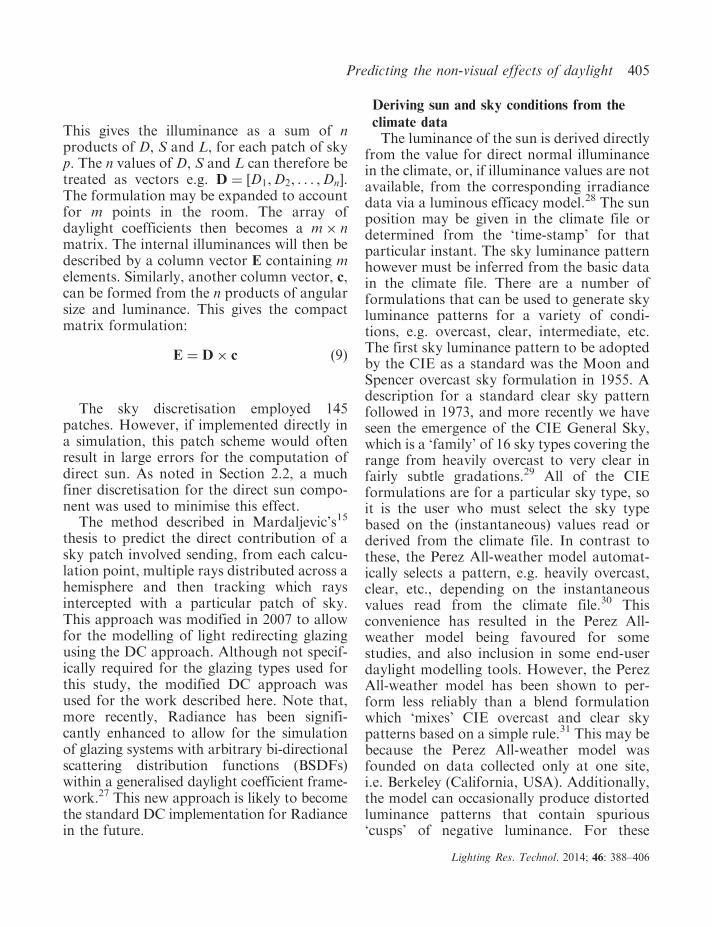
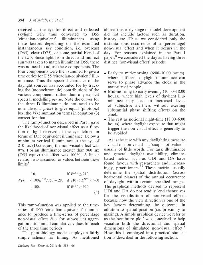
This gives the illuminance as a sum of nproducts of D, S and L, for each patch of skyp. The n values of D, S and L can therefore betreated as vectors e.g. D ¼ D1,D2, . . . ,Dn½ �.The formulation may be expanded to accountfor m points in the room. The array ofdaylight coefficients then becomes a m� nmatrix. The internal illuminances will then bedescribed by a column vector E containing melements. Similarly, another column vector, c,can be formed from the n products of angularsize and luminance. This gives the compactmatrix formulation:

E ¼ D� c ð9Þ

The sky discretisation employed 145patches. However, if implemented directly ina simulation, this patch scheme would oftenresult in large errors for the computation ofdirect sun. As noted in Section 2.2, a muchfiner discretisation for the direct sun compo-nent was used to minimise this effect.

The method described in Mardaljevic’s15

thesis to predict the direct contribution of asky patch involved sending, from each calcu-lation point, multiple rays distributed across ahemisphere and then tracking which raysintercepted with a particular patch of sky.This approach was modified in 2007 to allowfor the modelling of light redirecting glazingusing the DC approach. Although not specif-ically required for the glazing types used forthis study, the modified DC approach wasused for the work described here. Note that,more recently, Radiance has been signifi-cantly enhanced to allow for the simulationof glazing systems with arbitrary bi-directionalscattering distribution functions (BSDFs)within a generalised daylight coefficient frame-work.27 This new approach is likely to becomethe standard DC implementation for Radiancein the future.

Deriving sun and sky conditions from the

climate data

The luminance of the sun is derived directlyfrom the value for direct normal illuminancein the climate, or, if illuminance values are notavailable, from the corresponding irradiancedata via a luminous efficacy model.28 The sunposition may be given in the climate file ordetermined from the ‘time-stamp’ for thatparticular instant. The sky luminance patternhowever must be inferred from the basic datain the climate file. There are a number offormulations that can be used to generate skyluminance patterns for a variety of condi-tions, e.g. overcast, clear, intermediate, etc.The first sky luminance pattern to be adoptedby the CIE as a standard was the Moon andSpencer overcast sky formulation in 1955. Adescription for a standard clear sky patternfollowed in 1973, and more recently we haveseen the emergence of the CIE General Sky,which is a ‘family’ of 16 sky types covering therange from heavily overcast to very clear infairly subtle gradations.29 All of the CIEformulations are for a particular sky type, soit is the user who must select the sky typebased on the (instantaneous) values read orderived from the climate file. In contrast tothese, the Perez All-weather model automat-ically selects a pattern, e.g. heavily overcast,clear, etc., depending on the instantaneousvalues read from the climate file.30 Thisconvenience has resulted in the Perez All-weather model being favoured for somestudies, and also inclusion in some end-userdaylight modelling tools. However, the PerezAll-weather model has been shown to per-form less reliably than a blend formulationwhich ‘mixes’ CIE overcast and clear skypatterns based on a simple rule.31 This may bebecause the Perez All-weather model wasfounded on data collected only at one site,i.e. Berkeley (California, USA). Additionally,the model can occasionally produce distortedluminance patterns that contain spurious‘cusps’ of negative luminance. For these



reasons, the sky luminance patterns used forthis study were derived from blends of CIEskies.31

As noted in Section 2.3, the illuminationfrom the sun, overcast sky and clear sky wereassumed to correspond to, respectively, CIEstandard illuminants D55, D65 and D75. It isacknowledged that this is a crude approxima-tion. Whilst it might be possible in the futureto improve on the parameterisation of thispart of the model (e.g. a more suitablespectrum to approximate ‘blue skies’), it isunlikely that refinements to include, say, thevariation in spectrum across the sky vaultwould be worthwhile modelling. This isbecause uncertainties in, say, the spectralreflectance characteristics of external sur-faces, obstructions, etc. are likely to over-whelm what are probably subtle effects in theoverall model.

Annual simulations

A consequence of the definition of thedaylight coefficient is that, once computed, asingle set of DC matrices can be used toquickly simulate internal illuminances forarbitrary climates and arbitrary buildingorientations. Thus the approach is wellsuited for parametric studies. The procedureis as follows:

� Load pre-computed daylight coefficients.� Select climate file and assign a building

orientation.� For each time-step during daylight hours,

generate the appropriate sky luminancepattern and sun description according tothe values in the climate file and theorientation applied to the building.

� Derive internal illuminances from the pre-computed daylight coefficients and lumi-nance patch values derived in the previousstep.

� Process illuminance data applying themodel for non-visual effects and generatesummary metrics/graphics

Climate-based Daylight Modeling (CBDM)

software

The software used to carry out CBDMsimulations (employing Radiance as the‘engine’ to predict daylight coefficients) is abespoke research tool developed byMardaljevic. It exists as a collection of scriptsand procedures which are continually refined/updated in response to new challenges be theylive projects or purely theoretical/research innature. The software is a specialist tool withno graphical user interface, sparse documen-tation and continually changing. For thesereasons it has not been released and is usedsolely ‘in house’, though the key algorithmsetc. and various other details have beenpublished.

End-user CBDM tools include DAYSIM,32

DIVA4RHINO33 and OpenStudio34 – all useRadiance as the lighting ‘engine’. It is notknown if any of these tools could be useddirectly or adapted/configured by the user forthe climate-based modelling of non-visualeffects.



A framework for predicting the non-visual effects of daylight - Part I: photobiology- based model

Documents

Transcript of A framework for predicting the non-visual effects of daylight - Part I: photobiology- based model