Using Regression Analysis for Predicting Energy ...
82
Rochester Institute of Technology Rochester Institute of Technology RIT Scholar Works RIT Scholar Works Theses 5-2022 Using Regression Analysis for Predicting Energy Consumption in Using Regression Analysis for Predicting Energy Consumption in Dubai Police Dubai Police Amal Rashid Alqasim [email protected] Follow this and additional works at: https://scholarworks.rit.edu/theses Recommended Citation Recommended Citation Alqasim, Amal Rashid, "Using Regression Analysis for Predicting Energy Consumption in Dubai Police" (2022). Thesis. Rochester Institute of Technology. Accessed from This Master's Project is brought to you for free and open access by RIT Scholar Works. It has been accepted for inclusion in Theses by an authorized administrator of RIT Scholar Works. For more information, please contact [email protected].
-
Upload
khangminh22 -
Category
Documents
-
view
3 -
download
0
Transcript of Using Regression Analysis for Predicting Energy ...

Rochester Institute of Technology Rochester Institute of Technology
RIT Scholar Works RIT Scholar Works
Theses
5-2022
Using Regression Analysis for Predicting Energy Consumption in Using Regression Analysis for Predicting Energy Consumption in
Dubai Police Dubai Police
Amal Rashid Alqasim [email protected]
Follow this and additional works at: https://scholarworks.rit.edu/theses
Recommended Citation Recommended Citation Alqasim, Amal Rashid, "Using Regression Analysis for Predicting Energy Consumption in Dubai Police" (2022). Thesis. Rochester Institute of Technology. Accessed from
This Master's Project is brought to you for free and open access by RIT Scholar Works. It has been accepted for inclusion in Theses by an authorized administrator of RIT Scholar Works. For more information, please contact [email protected].

i
Using Regression Analysis for Predicting
Energy Consumption in Dubai Police
by
Amal Rashid Alqasim
A Capstone Submitted in Partial Fulfilment of the Requirements for
the Degree of Master of Science in Professional Studies: Data
Analytics
Department of Graduate Programs & Research
Rochester Institute of Technology
RIT Dubai
May 2022

i
RIT
Master of Science in Professional Studies:
Data Analytics
Graduate Capstone Approval
Student Name: Amal Rashid Alqasim
Graduate Capstone Title: Using Regression Analysis for Predicting Energy
Consumption in Dubai Police
Graduate Capstone Committee:
Name: Dr. Sanjay Modak Date:
Chair of committee
Name: Dr. Ehsan Warriach Date:
Member

ii
Acknowledgments
I would like to start with expressing my appreciation and gratitude to Dubai Police for
granting me access to the dataset that made complete this research. My warmest thanks to my
colleague at work Enaam for her constant support, encouragement and advice. My deepest
gratitude to my mentor Dr. Ehsan for his support and guidance throughout my work on the project.
In addition, to Rochester Institute of Technology Dubai and all my instructors for allowing me to
progress and develop my skills especially in R programming language. Finally, I would like to
give a special thanks to my family and friends for their constant source of inspiration, for believing
in me and encouraging me to reach my goals.

iii
Abstract
The aim of this project is to build a machine learning algorithm to forecast electricity and
water consumption for the 27 sites in Dubai Police facilities. This aim is to establish a central
database with all the data to monitor the energy consumption in a systematic manner and feed the
data in a visualized dashboard. The data was collected from the energy conservation department
at Dubai Police for five years from 2017 to 2021 comprising of electricity and water consumption
details data. Due to the numerous buildings and facilities any irregular behavior in consumption
takes time to be identified using conventional analysis methods, therefore this project will be able
to support the organization to find out their energy savings/loss hotspots and facilitate immediate
action for the employees to avoid time and monetary loss. Consumption data gathered will be
processed through R Programming language to break it down into quarter consumption for each
site. The Processed data for 2017 to 2020 will be an input for the multiple regression and ARIMA
models to forecast the quarter consumption of year 2021 and to showcase the model. Finally,
tableau software will be used to visualize the data and to build the dashboard in the future.
Keywords: Machine learning, Energy consumption prediction, Linear Regression Model, Autoregressive Integrated Moving
Average, Energy Forecasting

iv
Table of Contents
Contents
ACKNOWLEDGMENTS .................................................................................................................................... II
ABSTRACT ......................................................................................................................................................... III
LIST OF FIGURES ............................................................................................................................................. VI
LIST OF TABLES.............................................................................................................................................. VII
CHAPTER 1 ......................................................................................................................................................... 8
1.1 INTRODUCTION ................................................................................................................................... 8
1.2 PROJECT GOALS .................................................................................................................................. 9
RESEARCH QUESTIONS .............................................................................................................................................. 9
1.3 AIMS AND OBJECTIVES ...................................................................................................................... 9
1.4 RESEARCH METHODOLOGY .......................................................................................................... 10
1.5 LIMITATIONS OF THE STUDY ......................................................................................................... 11
CHAPTER 2 – LITERATURE REVIEW ......................................................................................................... 12
2.1 INTRODUCTION ................................................................................................................................. 12
2.2 LITERATURE REVIEW ...................................................................................................................... 12
2.2 CONCLUSION ...................................................................................................................................... 20
CHAPTER 3- PROJECT DESCRIPTION ........................................................................................................ 21
3.1 INTRODUCTION ................................................................................................................................. 21
3.2 DATA SOURCE ........................................................................................................................................... 22
3.3 DATA COLLECTION ................................................................................................................................. 22
3.3.1 ELECTRICITY AND WATER BILLS ...................................................................................................................... 22 3.3.2 FACILITIES LIST (THE FULL TABLE IS IN APPENDIX 1)...................................................................................... 23 3.3.3. CAPITA AND AREA LIST .................................................................................................................................. 24
CHAPTER 4- DATA ANALYSIS ...................................................................................................................... 26
4.1 DATA PREPARATION ............................................................................................................................... 26
4.2 DATA PREPROCESSING ........................................................................................................................... 26
4.2.1 DATA CLEANING ............................................................................................................................................. 26 4.2.2 DATA PREPARATION ....................................................................................................................................... 27
4.3 DATA QUALITY DIMENSIONS ................................................................................................................ 30
4.4 FEATURE ENGINEERING ........................................................................................................................ 31
4.5 CORRELATION BETWEEN ATTRIBUTES ............................................................................................ 34
4.6 VARIABLE DICTIONARY ......................................................................................................................... 35
4.7 DATA EXPLORATION AND VISUALIZATION ............................................................................... 36
v
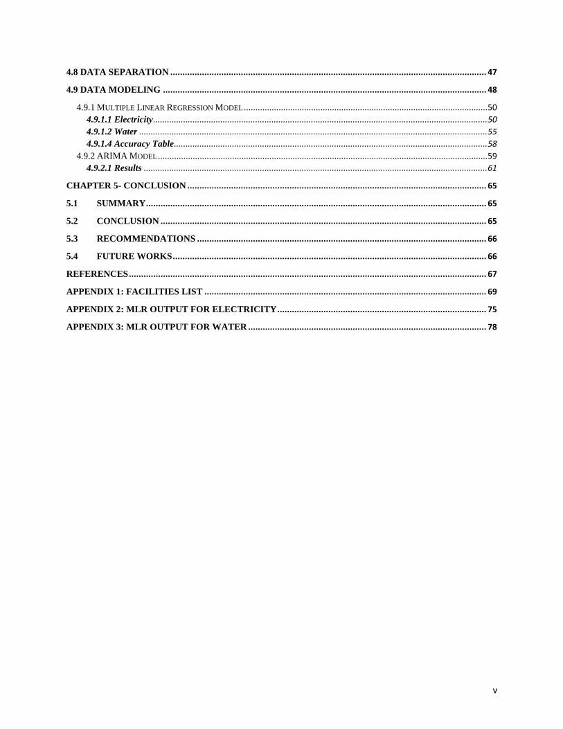
4.8 DATA SEPARATION .................................................................................................................................. 47
4.9 DATA MODELING ..................................................................................................................................... 48
4.9.1 MULTIPLE LINEAR REGRESSION MODEL ......................................................................................................... 50 4.9.1.1 Electricity ................................................................................................................................................ 50 4.9.1.2 Water ...................................................................................................................................................... 55 4.9.1.4 Accuracy Table ....................................................................................................................................... 58
4.9.2 ARIMA MODEL .............................................................................................................................................. 59 4.9.2.1 Results .................................................................................................................................................... 61
CHAPTER 5- CONCLUSION ........................................................................................................................... 65
5.1 SUMMARY ............................................................................................................................................ 65
5.2 CONCLUSION ...................................................................................................................................... 65
5.3 RECOMMENDATIONS ....................................................................................................................... 66
5.4 FUTURE WORKS ................................................................................................................................. 66
REFERENCES ................................................................................................................................................... 67
APPENDIX 1: FACILITIES LIST .................................................................................................................... 69
APPENDIX 2: MLR OUTPUT FOR ELECTRICITY ...................................................................................... 75
APPENDIX 3: MLR OUTPUT FOR WATER .................................................................................................. 78

vi
List of Figures Figure 1: Schematic presentation of the data analysis flow using SAS Enterprise Miner. .......................................... 14
Figure 2: Normalized predictive performance of single ANN, DT and hybrid model vs, normalized actual energy
data. ............................................................................................................................................................................. 16
Figure 3: The predictive power of the model............................................................................................................... 16
Figure 4: Correlation Matrix. ....................................................................................................................................... 34
Figure 5: Average Consumption by Division. ............................................................................................................. 36
Figure 6: Average Consumption Amount by Division. ............................................................................................... 36
Figure 7: Electricity Consumption by Year. ................................................................................................................ 37
Figure 8: Water Consumption by Year. ....................................................................................................................... 37
Figure 9: Electriciy Consumption by Month. .............................................................................................................. 37
Figure 10: Water Consumption by Month. .................................................................................................................. 37
Figure 11: Electricity consumption quarterly for year 2017. ....................................................................................... 38
Figure 12: Electricity consumption quarterly for year 2018. ....................................................................................... 38
Figure 13: Electricity consumption quarterly for year 2019. ....................................................................................... 38
Figure 14: Electricity consumption quarterly for year 2020. ....................................................................................... 38
Figure 15: Water consumption quarterly for year 2017. .............................................................................................. 39
Figure 16: Water consumption quarterly for year 2018. .............................................................................................. 39
Figure 17: Water consumption quarterly for year 2019. .............................................................................................. 39
Figure 18: Water consumption quarterly for year 2020. .............................................................................................. 39
Figure 19: Electricity Consumption trend. .................................................................................................................. 40
Figure 20: Water Consumption trend. ......................................................................................................................... 40
Figure 21: Electricity Consumption for each GHQ Department. ................................................................................ 41
Figure 22: Water Consumption for each GHQ Department. ....................................................................................... 41
Figure 23: Electricity Consumption per Area for all departments and PSs. ............................................................... 41
Figure 24: Electricity Consumption per Capita for all departments and PSs. ............................................................. 41
Figure 25: Water Consumption per Area for all departments and PSs. ....................................................................... 42
Figure 26: Water Consumption per Capita for all departments and PSs. .................................................................... 42
Figure 27: Electricity Consumption of Departments and PSs based on their Area Rank. ........................................... 43
Figure 28: Water Consumption of Departments and PSs based on their Area Rank. .................................................. 43
Figure 29: The trend of temperature and electricity consumption each quarter. ......................................................... 44
Figure 30: The trend of temperature and water consumption each quarter. ................................................................ 44
Figure 31: A quarterly report of electricity consumption for Al Riffa PS for the first Quarter. .................................. 45
Figure 32: A quarterly report of water consumption for Al Riffa PS for the first Quarter. ......................................... 45
Figure 33: Electricity Consumption for Airport Security Department for each quarter. ............................................. 46
Figure 34: Quarterly Electricity Consumption based on Area Ranking. ..................................................................... 46
Figure 35 : Residuals versus fitted values for electricity linear regression model. ...................................................... 52
Figure 36: QQ plot for electricity linear regression model. ......................................................................................... 52
Figure 37: Spread-Location graph for electricity linear regression model. ................................................................. 53
Figure 38: Residuals versus leverage plot for electricity linear regression model. ...................................................... 53
Figure 39: Predicted versus actual values for electricity linear regression model. ...................................................... 54
Figure 40: Residuals versus fitted values for water linear regression model. .............................................................. 56
Figure 41: QQ plot for water linear regression model. ................................................................................................ 56
Figure 42: Spread-Location graph for water linear regression model. ........................................................................ 56
Figure 43: Residuals versus leverage plot for water linear regression model. ............................................................. 57
Figure 44: Predicted versus actual values for water linear regression model. ............................................................. 58
Figure 45: Protective Security Emergency Department Electricity Consumption ARIMA Model. ............................ 61
vii
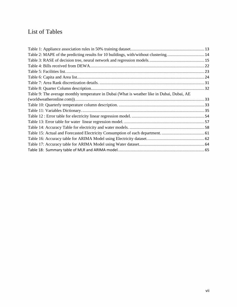
List of Tables
Table 1: Appliance association rules in 50% training dataset. .................................................................... 13
Table 2: MAPE of the predicting results for 10 buildings, with/without clustering. .................................. 14
Table 3: RASE of decision tree, neural network and regression models. ................................................... 15
Table 4: Bills received from DEWA. .......................................................................................................... 22
Table 5: Facilities list. ................................................................................................................................. 23
Table 6: Capita and Area list....................................................................................................................... 24
Table 7: Area Rank discretization details. .................................................................................................. 31
Table 8: Quarter Column description. ......................................................................................................... 32
Table 9: The average monthly temperature in Dubai (What is weather like in Dubai, Dubai, AE
(worldweatheronline.com)). ........................................................................................................................ 33
Table 10: Quarterly temperature column description. ................................................................................ 33
Table 11: Variables Dictionary. .................................................................................................................. 35
Table 12 : Error table for electricity linear regression model. .................................................................... 54
Table 13: Error table for water linear regression model. ........................................................................... 57
Table 14: Accuracy Table for electricity and water models. ...................................................................... 58
Table 15: Actual and Forecasted Electricity Consumption of each department. ........................................ 61
Table 16: Accuracy table for ARIMA Model using Electricity dataset. ..................................................... 62
Table 17: Accuracy table for ARIMA Model using Water dataset............................................................. 64
Table 18: Summary table of MLR and ARIMA model. ................................................................................ 65
8
Chapter 1
1.1 Introduction
It is evident that Dubai Police has evolved from a conventional policing services provider
to a world-leading organization that integrates safety and security with the community’s well-
being and happiness. And in line with the vision and direction of Dubai Police for utilizing artificial
intelligence through integrating software, Apps, and ML programs; implementing best energy
practices and measures is crucial at this point. In fact, this study focuses on the water and electricity
consumption of the police force across all its owned and occupied buildings/entities, with a main
focus of establishing a standard system for monitoring, reporting, as well as providing future
consumption predictions.
The current methodology for analyzing and monitoring the energy and water consumption
places several obstacles to get accurate results that are instant and allow for immediate action in
case of damages or leaks. It is worth mentioning that the consumption data reflects Greenhouse
Gases (GHG) emissions increments. Moreover, the first step in analyzing the consumption data is
to collect the bills from Dubai Electricity and Water Authority (DEWA) in quarterly basis in one
excel sheet containing contract number and consumption detail. The data collection process from
all the water and electricity meters under Dubai Police account turned out to be time consuming
and questionable due to the lack of a standard inventory system customized for consumption
meters and updated on monthly basis. The available excel sheets are numerous, duplicated and
contain inconsistent data that gave an alert and concern environmentally and financially.
Nevertheless, with the success of this project two standard ML algorithm will be created
to input all the data which will allow for instant analysis for all locations and highlight hotspots
(over consumers), to prevent unmonitored expenditures, generate annual comparisons that are
credible and accurate and build a forecasting model to predict future consumption. Upon
completion, once the project is proved functional and successful, it could be applied across the
organization for a better understanding of consumption data and as decision-making tool for the
energy conservation department at Dubai Police.
9
1.2 Project Goals
The Energy Conservation Department at Dubai Police generates quarterly electricity and
water consumption reports following the standards and guidelines of ISO 50001: 2018 for energy
management systems. Basically, it involves logging the quarterly water and electricity
consumption of the Dubai Police facilities, taking into account all the buildings that belong and
operate under the organization, and communicate to the head of each building to inform them
about their consumption and best practices. Therefore; the purpose is to analyze the consumption
data by using IoTs avoiding the use of time-consuming conventional methods, gather all previous
and current data in one database, visualize the data to stakeholders in a professional dashboard,
monitor consumption loss/savings hotspots sites to find out the causes and solutions based on their
frequency, and predict future consumption trends based on seasonal changes and other factors.
Additionally, this study will explore and add to previous literature conducted in this sector and
will be able to support in identifying the causes of high consumption in organizations.
Research questions
• What factors influence an inaccurate consumption data in any organization?
• What are the benefits of forecasting future consumptions for an organization?
• How does immediate detection of energy savings/loss hotspots impact the organization?
1.3 Aims and Objectives
Dubai Police is considered one of the largest government entities in the Emirate of Dubai
employing around 25% of the total of government employees. The Force is distributed among 30
sites in Dubai with more than 400 buildings operating round the clock to provide safety and
security for the community as well as achieving the lowest possible carbon footprint via energy
and resource efficiency initiatives. Over the years, the electricity and water consumed by Dubai
Police facilities to run its operations has proved to constitute the biggest environmental impact.
However, the analysis of the electricity and water consumption of Dubai Police facilities is carried
out manually using conventional methods which have resulted in generating inaccurate results and
consumed time in pinpointing areas of irregular high consumption that are out of the norm.
10
The main objectives of the project are to:
• Analyze electricity and water consumption data by using ML avoiding the use of time-
consuming methods.
• Implement DA tools to gather the data and create a forecasting model to predict electricity and
water consumption based on historical data.
• Publish quarter reports to be shared with each building operator showing a comparison between
their current and previous consumption including the percentage of savings/loss.
1.4 Research Methodology
For best results, it is recommended to use the CRISP-DM process. The stages are explained
in details below.
Stage 1: Business Understanding
Business Objective: The first step is to understand the objective and the problem the
organization needs to address.
The clients’ concerns are known and included in the problem statement. The organization
aims to conserve electricity and water consumption and reduce bills budget and this can be done
by building a machine-learning algorithm to monitor and detect hotspots and forecast future
consumption. The problem statement was shared with stakeholders and they confirmed that they
needed it and the data to be used for the study was provided by them.
Stage 2: Data Understanding
The actions to be done in this phase is to collect initial data, describe data, explore data,
and verify data quality. The data is evaluated to know how much it is relevant to the problem. The
collection of data will start with identifying Buildings/Facilities, followed by identifying
associated accounts/meters, and finally, determining the time period for the consumption data
needed. The data collected will contain more than 11 variables including facility name, months,
electricity consumption (kWh), and water consumption (Gallons) for five years from the period of
2017 to 2021. The data will be in different excel sheets, each sheet contains consumption details
as well as associated meter contract numbers for every year and one sheet mapping the meter
contract numbers with each site with the detailed description of every building in each site. The
data is fed in the master sheets in respected categories to identify the total number of meters
belonging to the study, to compare the consumption pattern over the past five years, and to

11
highlight the accounts that express alarming concerns. For instance, sudden high consumption
from a specific meter that usually has a low consumption pattern could indicate an overlooked
leak.
Stage 3: Data Preparation
Preprocessing the data is an essential process before inputting the data in ML algorithm.
This step will be done using Microsoft Excel and R Studio and it will include discarding
excluded/decommissioned accounts to identify concerning accounts, remove null values, zero
values, outliers, and duplicated meters. As well as changing the data type of some attributes.
Furthermore, merging the tables in consumptions datasheets with facilities table and Capita & Area
table. All data will be grouped and summed in quarter basis. The split of 70% trained and 30%
tested will be done before run the data in the model.
Stage 4: Modeling
In this stage, the processed data will be an input for the regression model using R
programming language to forecast the annual consumption for year 2021. Based on the literature
review among the prediction models, ARIMA models are one of the best-known models for time
series-based energy consumption prediction. Furthermore, Tableau and R will be used to visualize
the data in different plots.
Stage 5: Evaluation
In this final step, the results will be verified for validity and accuracy. The forecasted data
for year 2021 will be validated with the actual one. Additionally, the accuracy of the model will
be tested in this phase and any errors in its different types will be identified, and finally plots
showing the relationship between actual and predicted results will be generated.
1.5 Limitations of the Study
Due to the confidentiality and privacy policies of Dubai police as a policing entity, the
dataset was somehow limited. The number of visitors in each police station and department as well
as number of prisoners were not accessible that would have given a more accurate insight for the
consumption per capita and predicted values if it was added to capita attribute. In addition, due to
the lack of time, the area and number of employees data were not provided for all buildings. As a
consequence, such facilities were excluded from the study.

12
Chapter 2 – Literature Review
2.1 Introduction
The literature review conducted highlights important aspects discussed in some of previous
research papers and articles. Through this literature review, I was able to identify some minor gaps
in the literature that this study might be add to. Also, many variables are considered when
deciding which research are considered dropouts.
2.2 Literature Review
(Amasyali and El-Gohary, 2018) summarized data-driven building energy consumption
prediction studies. The studies focus on reviewing forecast ranges, data properties and data
preprocessing methods used, machine learning algorithms used for forecasting, and performance
metrics used for evaluation.
The scope of the study was categorized according to building type, temporal
granularity, and expected energy consumption type. Only 19% of these models focus on
residential buildings, and the remaining models focus on non-residential buildings, including
commercial and educational buildings. Most of these (57%) in these models are designed to
predict hourly energy usage, while 12%, 15%, 4%, and 12% of the models Focuses on sub-hourly
daily, monthly, and yearly usage. In terms of data types, most of these studies (67%) used real-
world data for model training and testing, while 19% and 14% of studies used simulation data and
public benchmark data, respectively. However, the majority (56%) of the data sizes in the
studies reviewed used records that were one month to one year long, and, 9% used datasets shorter
than 1 month. 31% have been using records for over a year.
The machine-learning algorithm was used to train the model using ANN and SVM,
respectively, in 47% and 25% of the studies. Only 4% of studies used decision
trees. Meanwhile, 24% of studies used other statistical algorithms such as MLR, OLS, and
ARIMA. To assess overall performance, 41%, 29%, and 16% of the studies reviewed evaluated
the model using CV, MAPE, and RMSE, respectively.
Another study done by (Nafil, Bouzi, Anoune and Ettalabi, 2020), the paper contrasts three
forecasting methods ARIMA (Autoregressive Integrated Moving Average), Temporal causality
modeling, and Exponential smoothing) to calculate the energy demand forecasts of Morocco in
2020.
They found that for the ARIMA model, the mean difference between the predicted and
actual values was significant (significance ~ 0). The forecast chart shows the deviation between
13
the predicted and actual values. Therefore, it is a rejected model. For exponential
smoothing, the mean difference between the predicted and actual values is not important
(significance = 0.782). This means that it is a good candidate model. However, forecast plots
show that electricity demand is stable over the next few years, which is not
realistic. Therefore, the exponential smoothing model is also rejected. For a temporal causal
relationship model, the mean difference between the predicted and actual values for the same year
is not that big (significance = 0.404). Therefore, there is no difference between the
actual value and the value predicted by the model. The forecast curve is also an accepted model
because it shows that electricity demand is increasing and seasonal effects (curve fluctuations) are
also known.
(Singh and Yassine, 2018) presented an intelligent data mining model to analyze, forecast
and visualize energy time series to energy consumption patterns. Unsupervised data clustering,
frequent pattern mining analysis of energy time series, and Bayesian network prediction were used
to predict energy consumption. The accuracy results of identifying device usage patterns using the
proposed model outperformed Support Vector Machine (SVM) and Multilayer Perceptron (MLP)
at each stage, but 25%, 50%, and. Each reached 75% of the training data size. In addition, they
achieved prediction accuracy of energy consumption of 81.89% in the short term (hourly) and
75.88%, 79.23%, 74.74%, 72.81% in the long term. Semester; that is, day, week, month, season.
I noticed that devices such as laptops, monitors and speakers have associations. And as incremental
mining continues, the associations between these devices will be strengthened and new devices
such as washing machines, kettles and pedestrians will develop the associations. Residents enjoy
working on computers and listening to music while washing clothes, and working on computers
and riding trains while cooking, as a result of these interactions. You can deduce the occupants'
behavioral preferences.
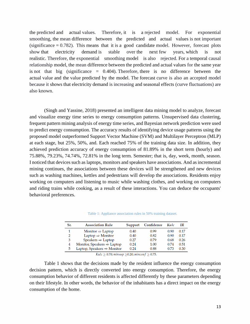
Table 1: Appliance association rules in 50% training dataset.
Table 1 shows that the decisions made by the resident influence the energy consumption
decision pattern, which is directly converted into energy consumption. Therefore, the energy
consumption behavior of different residents is affected differently by these parameters depending
on their lifestyle. In other words, the behavior of the inhabitants has a direct impact on the energy
consumption of the home.
14
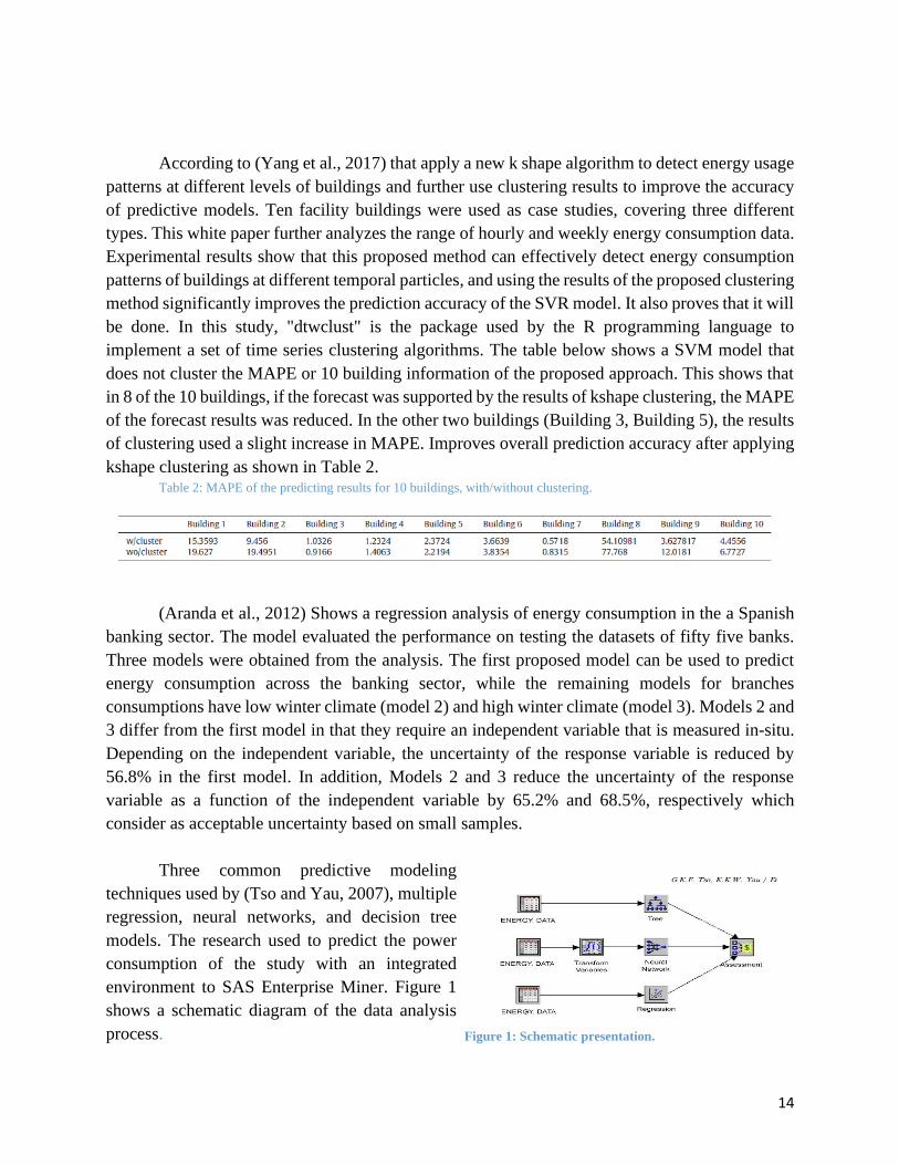
According to (Yang et al., 2017) that apply a new k shape algorithm to detect energy usage
patterns at different levels of buildings and further use clustering results to improve the accuracy
of predictive models. Ten facility buildings were used as case studies, covering three different
types. This white paper further analyzes the range of hourly and weekly energy consumption data.
Experimental results show that this proposed method can effectively detect energy consumption
patterns of buildings at different temporal particles, and using the results of the proposed clustering
method significantly improves the prediction accuracy of the SVR model. It also proves that it will
be done. In this study, "dtwclust" is the package used by the R programming language to
implement a set of time series clustering algorithms. The table below shows a SVM model that
does not cluster the MAPE or 10 building information of the proposed approach. This shows that
in 8 of the 10 buildings, if the forecast was supported by the results of kshape clustering, the MAPE
of the forecast results was reduced. In the other two buildings (Building 3, Building 5), the results
of clustering used a slight increase in MAPE. Improves overall prediction accuracy after applying
kshape clustering as shown in Table 2. Table 2: MAPE of the predicting results for 10 buildings, with/without clustering.
(Aranda et al., 2012) Shows a regression analysis of energy consumption in the a Spanish
banking sector. The model evaluated the performance on testing the datasets of fifty five banks.
Three models were obtained from the analysis. The first proposed model can be used to predict
energy consumption across the banking sector, while the remaining models for branches
consumptions have low winter climate (model 2) and high winter climate (model 3). Models 2 and
3 differ from the first model in that they require an independent variable that is measured in-situ.
Depending on the independent variable, the uncertainty of the response variable is reduced by
56.8% in the first model. In addition, Models 2 and 3 reduce the uncertainty of the response
variable as a function of the independent variable by 65.2% and 68.5%, respectively which
consider as acceptable uncertainty based on small samples.
Three common predictive modeling
techniques used by (Tso and Yau, 2007), multiple
regression, neural networks, and decision tree
models. The research used to predict the power
consumption of the study with an integrated
environment to SAS Enterprise Miner. Figure 1
shows a schematic diagram of the data analysis
process. Figure 1: Schematic presentation.

15
The target value is the total power consumption (kWh) for one week. Home types, home
characteristics, and device ownership are considered to be factors that can affect power
consumption.
Table 3: RASE of decision tree, neural network and regression models.
In the summer season, the decision tree model showed a better performance than the other
two methods. However, in the winter season, the neural network performed better. For comparison,
Table 6 summarizes the key factors identified in these models of energy consumption patterns and
energy consumption projections.
(Banihashemi, Ding and Wang, 2017) published a paper representing a hybrid model of a
machine learning algorithm that optimizes the energy consumption of houses, considering both
continuous energy parameters and discrete energy parameters at the same time. This study shows
a hybrid objective function of a machine learning algorithm that optimizes the energy consumption
of a house using an artificial neural network as a prediction model, and a classification algorithm
(decision tree) is used to create a hybrid function via a cross-training ensemble equation. The
model was finally validated via a weighted average of the errors decomposed for performance.
This research contributes to this field in various ways. It produces predicted energy consumption
data with minimal error and the highest accuracy for the purpose of developing hybrid objective
functions. This paves the way for presenting a powerful engine for building energy optimization.
The result is an integrated platform that incorporates both qualitative and quantitative variables of
building energy consumption without compromising data consistency or requiring data conversion
techniques. Due to the many limitations of conducting this study, the study results should be treated
with caution. This means that different hybrid models can emphasize different attributes, so the
results may not be directly applicable to other types of machine learning algorithms in prediction
and classification.
16
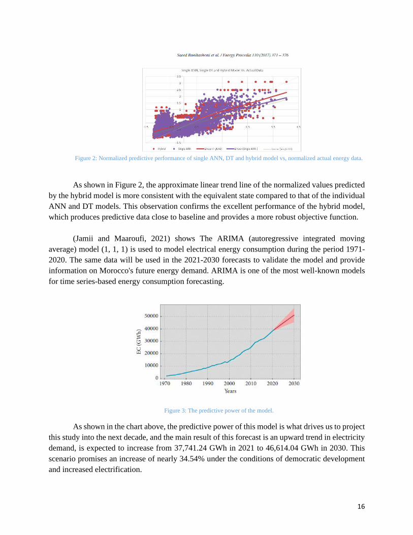
Figure 2: Normalized predictive performance of single ANN, DT and hybrid model vs, normalized actual energy data.
As shown in Figure 2, the approximate linear trend line of the normalized values predicted
by the hybrid model is more consistent with the equivalent state compared to that of the individual
ANN and DT models. This observation confirms the excellent performance of the hybrid model,
which produces predictive data close to baseline and provides a more robust objective function.
(Jamii and Maaroufi, 2021) shows The ARIMA (autoregressive integrated moving
average) model (1, 1, 1) is used to model electrical energy consumption during the period 1971-
2020. The same data will be used in the 2021-2030 forecasts to validate the model and provide
information on Morocco's future energy demand. ARIMA is one of the most well-known models
for time series-based energy consumption forecasting.
Figure 3: The predictive power of the model.
As shown in the chart above, the predictive power of this model is what drives us to project
this study into the next decade, and the main result of this forecast is an upward trend in electricity
demand, is expected to increase from 37,741.24 GWh in 2021 to 46,614.04 GWh in 2030. This
scenario promises an increase of nearly 34.54% under the conditions of democratic development
and increased electrification.
17
In the (Wang and Meng, 2012) study, a Hybrid Neural Network and ARIMA Model for
Energy Consumption Forecasting is used. Because the ARIMA model can't handle nonlinear
relationships, and the neural network model can't handle both linear and nonlinear patterns equally
well, to take advantage of the distinctive strengths as ARIMA in linear modeling and ANN in
nonlinear modeling. The empirical results using energy consumption data from Hebei province in
China show that the hybrid model can be a useful tool for improving the accuracy of energy
consumption forecasting obtained using either of the models alone. Three statistical measures are
used to evaluate each model's predicting performance: RMSE, MAE, and MAPE. The statistical
metrics show that the hybrid model can be a useful tool for improving the forecasting accuracy of
either of the models when employed alone.
(Sen, Roy and Pal, 2016) Shows an Indian pig iron manufacturing company using ARIMA
to predict energy usage and greenhouse gas emissions. The autoregressive integrated moving
average (ARIMA) is used for forecasting, and to see which ARIMA model is the best fit model
for energy consumption. Selecting the appropriate ARIMA models for these indicators will aid in
accurate forecasting. While the ARIMA (0,1,0) (0,1,1) model has an AICC of -8.033 and an SBIC
of 8.013 for energy consumption, the ARIMA (0,1,4) (0,1,1) model has an AICC of -8.109 and an
SBIC of 8.068. In terms of energy usage, the second [i.e. ARIMA (1,0,0) (0,1,1)] model is
unquestionably superior to the first [i.e. ARIMA (0,1,0) (0,1,1)] model, as all key indices show
lower values.
A model based on the k-means algorithm was built for this goal in the paper Big Data
Analytics for Discovering Electricity Consumption Patterns in Smart Cities (Pérez-Chacón et al.,
2018). This research yielded two possible values for the number of clusters, and both cases were
subjected to an in-depth investigation of the patterns. The patterns were classified by the type of
consumption (high, low, etc.), the season of the year, and the day of the week. Building
consumption behavior is mostly determined by their nature (administrative buildings, research
centers, schools, or recreational facilities) and the hours of use during the day. Furthermore, it has
been established that there is a strong link between temperature and consumption, as well as a
significant impact on vacation seasons.
In (Yuan, Liu and Fang, 2016) study a Comparison of China's primary energy consumption
forecasting by using the ARIMA model and GM (1,1) model was done. China's primary energy
consumption is forecasted using two univariate models: ARIMA and GM (1,1). The two models'
findings are in line with the specifications. The fitted values of the ARIMA model respond less to
fluctuations since they are restricted by its long-term trend, whereas the fitted values of the GM
(1,1) model respond more due to the use of the most recent four data. According to the Wilcoxon
signed-rank test, the residues of the two models are statistically opposite. As a result, a hybrid
18
model is created using these two models, with a MAPE (Mean Absolute Percent Error) that is
lower than the ARIMA and GM (1,1) models. The three models are then used to forecast China's
primary energy consumption.
Accurately estimating energy use in public buildings is an important method for reducing
energy demand and increasing energy efficiency. The goal of this research (Liu et al., 2020) was
to provide a novel method for predicting energy usage in public buildings. Small samples, high-
dimensional, and nonlinear issue forecasts are all good candidates for the SVM approach. The
prediction effect of the average relative error is 5.03 percent in the case analysis of daily building
energy consumption prediction, and the practicality of the energy vector prediction method based
on the SVM method is confirmed. It has been discovered that when the difference between the
actual and anticipated values is more than the test set's maximum error, the energy consumption is
abnormal.
The algorithm of the prediction model in this study (Shapi, Ramli and Awalin, 2021) is
proposed using three methodologies: Support Vector Machine, Artificial Neural Network, and k-
Nearest Neighbor. Two tenants from a business building are used as a case study to demonstrate
real-life applicability in Malaysia. The energy demand data obtained from June to December 2018
was evaluated and pre-processed for predictive model training and testing. The SVM method
yielded the most promising results, as it was the best method for two tenants, with RMSE values
of 4.7506789 and 3.5898263, respectively. Furthermore, SVM results show a lower mean absolute
error for 12.09 and 43.97, respectively, whereas k-NN results show a lower RMSE for these two
tenants. SVM predicted demand also performed better when average consumption was calculated
from demand, achieving a lower MAPE than the other methods for all tenants.
In this study (Zhao and Magoulès, 2012), two feature selection methods are used to predict
energy consumption, which is then tested on three data sets using support vector regression. The
two filter methods used are gradient-guided feature selection and correlation coefficients, which
can assign a score to each feature based on its usefulness to the predictor. The experimental results
confirm the validity of the chosen subset and demonstrate that the proposed feature selection
method guarantees prediction accuracy while reducing computational time for data analysis.
In this paper (de Oliveira and Cyrino Oliveira, 2018), ARIMA methods are used to analyze
monthly electric energy consumption time series from various countries. The findings indicate that
the proposed methodologies significantly improve the forecast accuracy of demand for energy end-
use services in both developed and developing countries. It should be noted that external factors
account for a significant portion of the variation in monthly electric energy consumption, which
cannot be captured by univariate forecasting methods. Some notable examples include the effects
of electric energy generation and, in particular, industrial output in several countries.

19
(Carrera, Peyrard and Kim, 2021) Shows a three-months-ahead prediction problem for a
short-term stacking ensemble model for energy consumption in Songdo, South Korea. To achieve
this result, they first designed baseline regressors for prediction, then applied a three-combination
of each best model of the baseline regressors, and finally, a weighted meta-regression model was
applied using meta-XG Boost. The resulting model is known as the stacking ensemble model. The
proposed stacking ensemble model combines the best ensemble networks to improve performance
prediction, resulting in an R2 value of 97.89%. The results validate the efficacy of the ensemble
networks, which employ Artificial Neural Networks (ANN), Cat Boost, and Gradient Boosting. In
terms of R2, MAE, and RSME, the weighted meta-model outperforms several machine learning
models, according to this study.
When compared to other statistical models, the linear regression analysis has shown best
performance due to its reasonable accuracy and relatively simple implementation. Simple and
multiple linear regression analyses, as well as quadratic regression analyses, were performed on
hourly and daily data from a research house in this study (Fumo and Rafe Biswas, 2015). The
observed data's time interval proved to be an important factor in determining the model's quality.
Simple linear regression analysis was performed for time intervals of 5 and 15 minutes, yielding
R2 values of 0.232 and 0.384, respectively, to verify this statement. These additional findings
confirm that higher resolution for the analytical time interval leads to lower-quality models.
This paper (Wang, 2022) enhances the combined model I, which directly adds the ARIMA
model's projected value with the BP neural network model's anticipated value. The independent
variables are the ARIMA model's linear fitting and the BP model's nonlinear fitting, while the
dependent variable is the per capita coal consumption sequence. A new combination model II is
created using multiple linear regression. The combination model II is used to fit the per capita coal
consumption from 2014 to 2018 based on a study of the changing rule of China's per capita coal
consumption over time. The fitting errors are 0.62 percent, 0.17 percent, 0.04 percent, 0.04 percent,
and 0.07 percent, respectively, according to the results. The combined model II enhances the
forecast accuracy over the combined model I. ARIMA model fitting reduces the error of prediction
of per capita coal consumption, and BP model fitting predicts the ARIMA model fitting error. The
two models together reduce prediction error even further, and the combined model has a greater
overall prediction effect.
The annual energy consumption of Iran is estimated in this research (Barak and Sadegh,
2016) utilizing three ARIMA–ANFIS patterns. In the first pattern, the ARIMA model is applied
to four input features, and its nonlinear residuals are predicted using six different ANFIS (Adaptive
Neuro Fuzzy Inference System) structures, such as sub clustering, and means clustering, and grid
partitioning. In the second pattern, ARIMA forecasting is assumed as an input variable for ANFIS
prediction, along with four input features. As a result, in addition to ARIMA's output, four more
20
inputs are used in energy prediction with six alternative ANFIS structures. Due to data scarcity,
the second pattern is combined with the AdaBoost (Adaptive Boosting) data diversification model
in the third pattern, resulting in a novel ensemble methodology. The results show that the third
hybrid pattern, which combines the AdaBoost method with the Genfis3 ANFIS structure and the
backpropagation training procedure, produces better results, with the model's MSE criterion
dropping to 0.026 percent from 0.058 percent in the second hybrid pattern.
2.2 Conclusion In summary, among the eight papers in the literature review where in each more than one
model was used. Eighteen regression models were used with their different types (ARIMA,
Multiple Linear Regression, SVM...). However, two researches used Decision Tree, seven
researches Artificial Neural Network, and three research K- clustering. Another important point,
in the literature covered in this study, all hybrid models showed a better performance than every
single model. In general, regression models have proved the best performance comparing with
other models. Regarding the performance evaluation metrics, mostly RMSE, MAE, and MAPE
were used.

21
Chapter 3- Project Description
3.1 Introduction
Dubai Police is considered one of the largest government entities in the Emirate of Dubai
employing around 25% of the total of government employees. The Force is distributed among 30
sites in Dubai with more than 400 buildings operating round the clock to provide safety and
security for the community as well as achieving the lowest possible carbon footprint via energy
and resource efficiency initiatives. Over the years, the electricity and water consumed by Dubai
Police facilities to run its operations has proved to constitute the biggest environmental impact.
However, the analysis of the electricity and water consumption of Dubai Police facilities is carried
out manually using conventional methods which have resulted in generating inaccurate results and
consumed time in pinpointing areas of irregular high consumption that are out of the norm.
The first step of the project is to gather and collect the data from different sources. Then,
data cleaning and preprocessing will take place. The cleaned dataset will be gathered in a quarterly
basis and separated to 70:30 ratio to be input in the model. Two models will be run and compared.
The first model, a multiple regression model including many independent variables (Year, Quarter,
Capita, Area, etc.) to forecast the consumption of electricity and water separately. The second
model is univariate ARIMA model for each of electricity and water data. Both models will be done
to run the data of year 2017 to 2020 and forecast year 2021 consumption in quarterly basis.
Finally, the model’s performance evaluation metrics will be evaluated showing a table
compare the actual and predicted consumption.
22
3.2 Data Source
Electricity and water consumption data that will be used is taken from the meter substations
provided by DEWA to the organization. The data is then collected from the energy conservation
department at Dubai Police consisting of around 10 variables including contract account name,
Calendar month, electricity consumption (kWh) and water consumption (Gallons) for five years
from the period of 2017 to 2021. Also, to assign each contract number to its department or police
station, facilities list assigned to each contract number was collected also from properties
department. As well as, data of area and number of employees in each location was collected from
maintenance and HR departments. The three datasets will be combined and used for the model.
The dataset includes null values, zero values and repetitive values which will be cleaned using
techniques that enable us to input the dataset in different machine learning algorithms.
3.3 Data Collection
The energy conservation department in Dubai Police is receiving the monthly bills from Dubai
Water and Electricity Authority (DEWA) quarterly. Bills from 2017 to 2021 were combined in
one datasheet. In addition, the list of facilities mapped to the contract number is provided by the
properties department in Dubai Police. Also, the effect of the number of employees and building
areas on electricity and water consumption will be studied. The three datasets need to be
combined to create one datasheet and run the model based on it. A sample of each dataset will
be shown in the bellow sections.
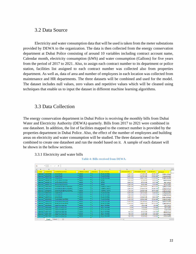
3.3.1 Electricity and water bills Table 4: Bills received from DEWA.
23
This excel sheet is a sample of the quarterly bills received from DEWA. It is composed of 10
columns and 17873 rows (for years from 2017 to 2021). The dataset contains many data for private and
unneeded accounts and some columns will not be needed for our study, like the “collective contract”
column. As the study will be for Dubai Police departments and police stations, any unnecessary or irrelevant
facilities will be removed from the data.
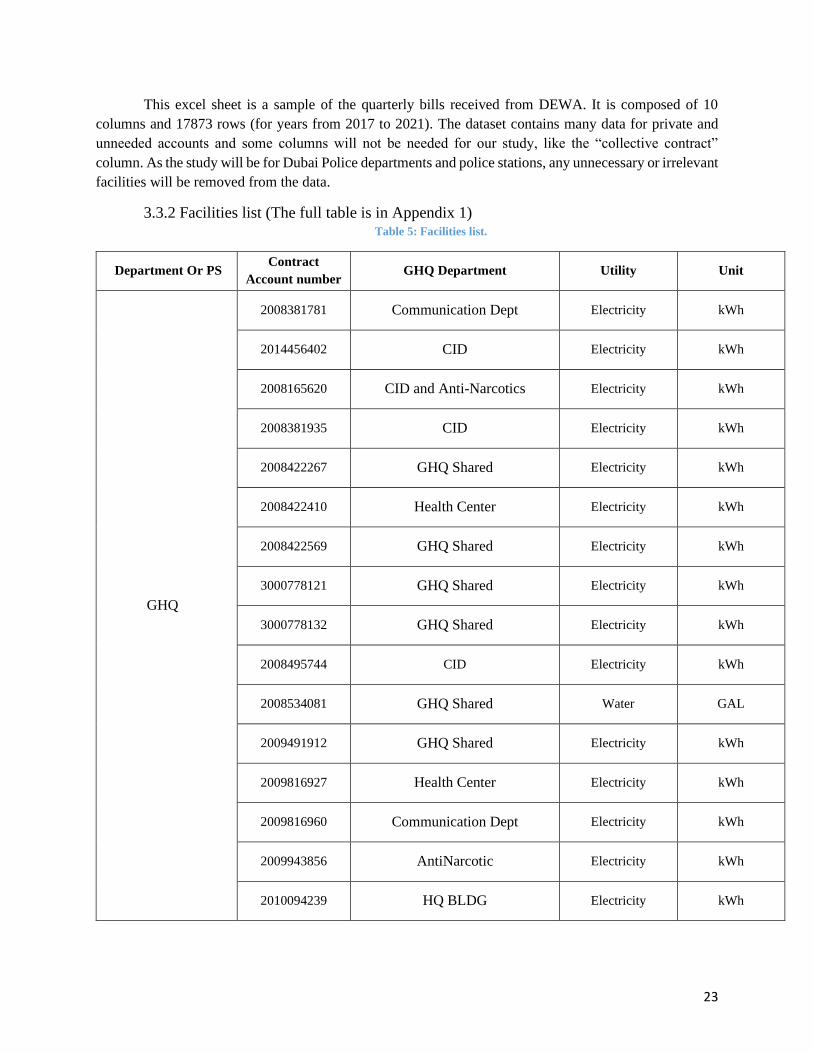
3.3.2 Facilities list (The full table is in Appendix 1) Table 5: Facilities list.
Department Or PS Contract
Account number GHQ Department Utility Unit
GHQ
2008381781 Communication Dept Electricity kWh
2014456402 CID Electricity kWh
2008165620 CID and Anti-Narcotics Electricity kWh
2008381935 CID Electricity kWh
2008422267 GHQ Shared Electricity kWh
2008422410 Health Center Electricity kWh
2008422569 GHQ Shared Electricity kWh
3000778121 GHQ Shared Electricity kWh
3000778132 GHQ Shared Electricity kWh
2008495744 CID Electricity kWh
2008534081 GHQ Shared Water GAL
2009491912 GHQ Shared Electricity kWh
2009816927 Health Center Electricity kWh
2009816960 Communication Dept Electricity kWh
2009943856 AntiNarcotic Electricity kWh
2010094239 HQ BLDG Electricity kWh

24
2010094980 HQ BLDG Electricity kWh
2010097041 HQ BLDG Electricity kWh
2010097106 HQ BLDG Electricity kWh
2010097130 HQ BLDG Electricity kWh
Al Riffa Police
Station
2008892646 Electricity kWh
2008892875 Electricity kWh
2009055420 Water GAL
2009222180 Electricity kWh
The above excel sheet is a sample of the facilities list for each contract number taken from the
properties department in Dubai Police. It is composed of 5 columns and 208 rows showcasing the facilities
that will be included in the study.
3.3.3. Capita and Area list Table 6: Capita and Area list.
Facilities Capita
Area (meter
square)
GHQ Campus 3072 172,397
Dubai Police Academy 1234 168,385
Punitive and Correctional Establishments 5808 114,040
Al Wasl Protective Security and Emergency 543 40,234
Barsha Police Station 332 31,624
Officers Club 264 28,985
General Department of Transport and Rescue 898 32,528
Naif Police Station 345 11,887
K9 85 10,176
Nad Alsheba Police Station 988 11,816
Al Rashdiyah Police Station 363 12,895
Al Riffa Police Station 79 14,805
Moraqabat Police Station 350 21,794
Port Police Station 483 11,271

25
Traffic Department Deira 642 11,297
Barsha Traffic Dept 262 12,226
Bur Dubai Police Station 480 9,278
Qusais Police Station 344 9,353
Airport Security 1985 7,394
Awir Horse Stables 130 6,364
Hor Al Anz Protective Security and Emergency 124 4,187
Lahbab Police station 87 726
Hatta Police Station 186 1,086
Al Faqqa Police Station 11 1,406
Qusais Horse Stables 1,826
Qusais Warehouses 4 3,610
Jabal Ali Police Station 236 4,447
Rowaiyah Shooting Range 51 2,343
The number of employees and the area of each facility is described in the above table. The gathered
data is for 28 facilities, however, the data for 5 facilities were not provided due to confidentiality reasons.
Although that shouldn’t stop us from including these two variables as it will add a good value to the model.
This table contains 29 rows and 3 columns.
26
Chapter 4- Data Analysis
4.1 Data Preparation
First of all, we need to add all bills for all quarters from 2017 to 2021 in one sheet (a total of 17,873
rows). Then, we need to merge all the required data. This was done using the “left_join” function in R.
Facilities list will be joined with bills data sheet based on “contract number” and “Division” to get two
more columns (DepartmentOrPS and GHQ Department). Then, we will join capita and area based on the
DepartmentOrPS column.
4.2 Data Preprocessing
4.2.1 Data Cleaning
The cleaning process was conducted in Microsoft Excel and R Studio. The bills received
from DEWA contain many duplicates, zero values, Na’s, unknown locations, and unnecessary
accounts. I followed these cleaning steps before we start joining the three datasets together:
Below are the cleaning steps for the bill’s datasheet:
Microsoft Excel:
• Compile all year’s bills together (monthly basis from January to December)
• Prepare datasheet for locations with their meter numbers (Contract Account)
• Add a new column for years to distinguish which year each consumption is assigned.
• Remove the units from the Consumption unit and Consumption Amount columns. Units
are affecting the variable type in R so it's difficult to deal with them as numeric. As we
have a column (Division) describing each row if it is assigned to “Electricity” or “Water”
keeping the units is useless.
R Studio:
• Removing NAs, blanks, and zero values in Bills dataset.
- Removing NAs and zero values in the “Consumption.Unit” column.
There are 210 NA values and 1160 Zero values in the Consumption.unit. As all the study
is based on this variable so it is not logical to keep zero values in this column. As it is impossible
27
to have zero consumption for a working meter unless they closed a building for at least 1 month.
And even if it does happen, we will not need this information for the study.
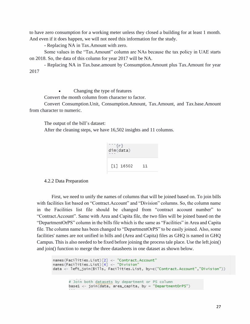
- Replacing NA in Tax.Amount with zero.
Some values in the “Tax.Amount” column are NAs because the tax policy in UAE starts
on 2018. So, the data of this column for year 2017 will be NA.
- Replacing NA in Tax.base.amount by Consumption.Amount plus Tax.Amount for year
2017
• Changing the type of features
Convert the month column from character to factor.
Convert Consumption.Unit, Consumption.Amount, Tax.Amount, and Tax.base.Amount
from character to numeric.
The output of the bill’s dataset:
After the cleaning steps, we have 16,502 insights and 11 columns.
4.2.2 Data Preparation
First, we need to unify the names of columns that will be joined based on. To join bills
with facilities list based on “Contract.Account” and “Division” columns. So, the column name
in the Facilities list file should be changed from “contract account number” to
“Contract.Account”. Same with Area and Capita file, the two files will be joined based on the
“DepartmentOrPS” column in the bills file which is the same as “Facilities” in Area and Capita
file. The column name has been changed to “DepartmentOrPS” to be easily joined. Also, some
facilities' names are not unified in bills and (Area and Capita) files as GHQ is named in GHQ
Campus. This is also needed to be fixed before joining the process tale place. Use the left.join()
and join() function to merge the three datasheets in one dataset as shown below.
28
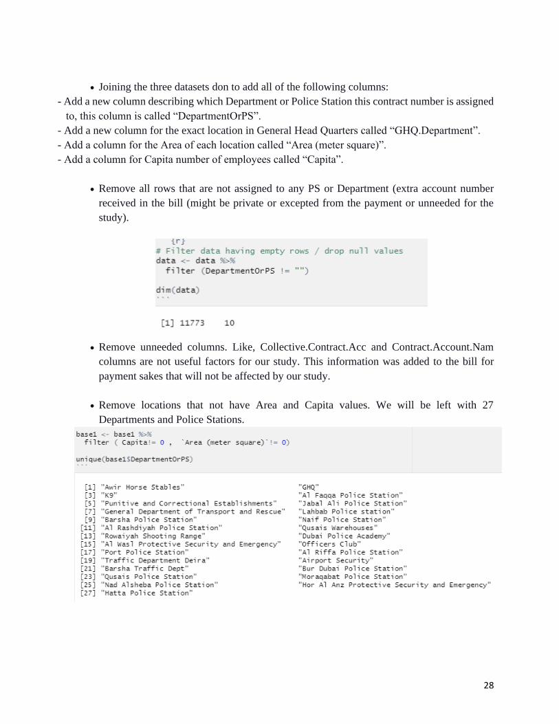
• Joining the three datasets don to add all of the following columns:
- Add a new column describing which Department or Police Station this contract number is assigned
to, this column is called “DepartmentOrPS”.
- Add a new column for the exact location in General Head Quarters called “GHQ.Department”.
- Add a column for the Area of each location called “Area (meter square)”.
- Add a column for Capita number of employees called “Capita”.
• Remove all rows that are not assigned to any PS or Department (extra account number
received in the bill (might be private or excepted from the payment or unneeded for the
study).
• Remove unneeded columns. Like, Collective.Contract.Acc and Contract.Account.Nam
columns are not useful factors for our study. This information was added to the bill for
payment sakes that will not be affected by our study.
• Remove locations that not have Area and Capita values. We will be left with 27
Departments and Police Stations.
29
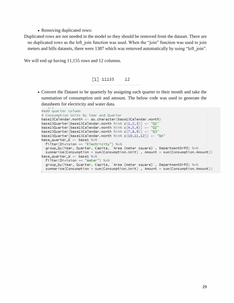
• Removing duplicated rows:
Duplicated rows are not needed in the model so they should be removed from the dataset. There are
no duplicated rows as the left_join function was used. When the “join” function was used to join
meters and bills datasets, there were 1387 which was removed automatically by using “left_join”.
We will end up having 11,155 rows and 12 columns.
• Convert the Dataset to be quarterly by assigning each quarter to their month and take the
summation of consumption unit and amount. The below code was used to generate the
datasheets for electricity and water data.

30
4.3 Data Quality Dimensions
To check data quality, we need to look at its six dimensions. The explanation of each is
mentioned below:
1. Completeness: the dataset has missing values and is set as NA or blanks as well as zero
consumption values. Facilities area and capita values are not provided. To overcome any
incompleteness in the datasets, we removed these facilities from the model.
2. Conformity: The facilities list received from the properties department names the facility
different than the table provided for Area and Capita for each facility. This needs to be
unified before joining the two datasets together.
3. Consistency: To make sure the bill amount (Tax.base.Amount) column received from
DEWA is equal to Consumption.amount plus Tax.amount. A new column was created to
check if they are consistent. The result was that our dataset is consistent.
4. Accuracy: The dataset was taken directly from the concerned department in Dubai Police.
This makes us sure that it is accurate. However, the Temperature column added was for
the temperature detected in Dubai City not specifying the year. If it has been found for the
exact location and each year and quarter it will be more accurate.
5. Duplicates: Duplicates can’t be applied to each column. As the dataset contains the
consumption data for the same “Contract Numbers” repeated for different years and moth.
The only duplicates we should avoid is having the same electricity/water consumption
duplicated for the same facility “Contract Number” recorded in the same year and month.
As this case was checked, the datasets do not contain any duplicates.
6. Integrity: The dataset is integrated and connected very well. When we joined the three
datasets together based on specific attributes that confirm that all attributes are related and
connected.
31
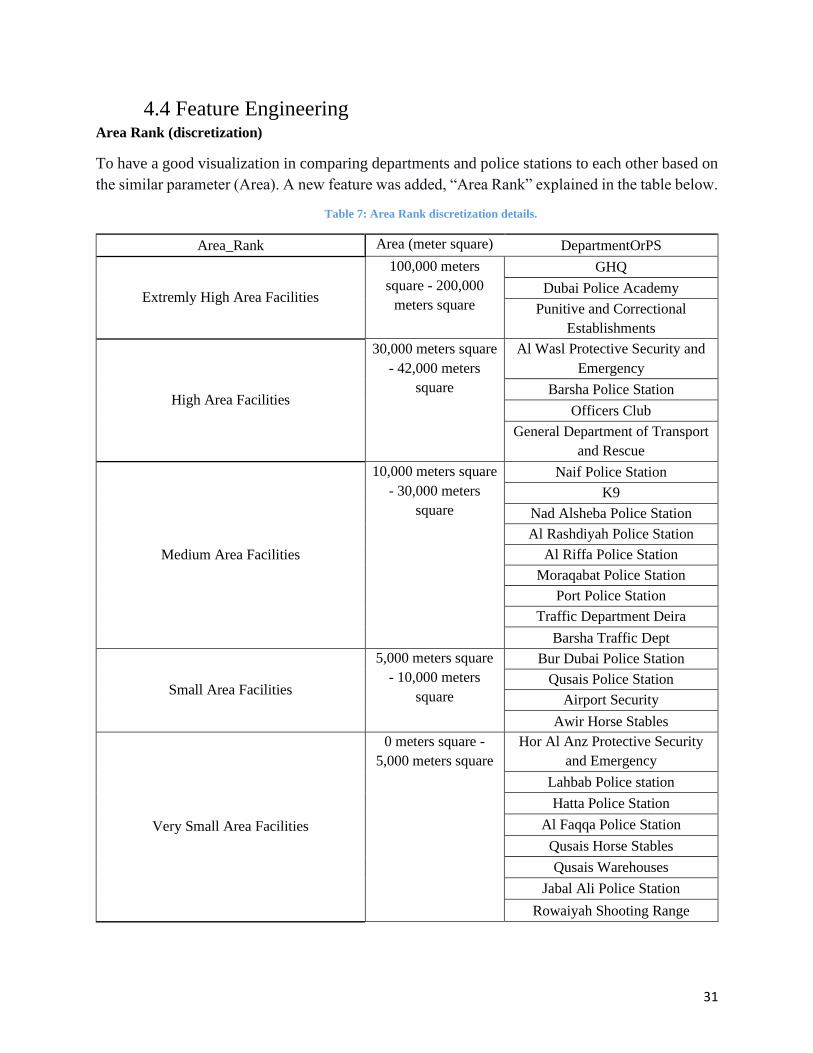
4.4 Feature Engineering Area Rank (discretization)
To have a good visualization in comparing departments and police stations to each other based on
the similar parameter (Area). A new feature was added, “Area Rank” explained in the table below.
Table 7: Area Rank discretization details.
Area_Rank Area (meter square) DepartmentOrPS
Extremly High Area Facilities
100,000 meters
square - 200,000
meters square
GHQ
Dubai Police Academy
Punitive and Correctional
Establishments
High Area Facilities
30,000 meters square
- 42,000 meters
square
Al Wasl Protective Security and
Emergency
Barsha Police Station
Officers Club
General Department of Transport
and Rescue
Medium Area Facilities
10,000 meters square
- 30,000 meters
square
Naif Police Station
K9
Nad Alsheba Police Station
Al Rashdiyah Police Station
Al Riffa Police Station
Moraqabat Police Station
Port Police Station
Traffic Department Deira
Barsha Traffic Dept
Small Area Facilities
5,000 meters square
- 10,000 meters
square
Bur Dubai Police Station
Qusais Police Station
Airport Security
Awir Horse Stables
Very Small Area Facilities
0 meters square -
5,000 meters square
Hor Al Anz Protective Security
and Emergency
Lahbab Police station
Hatta Police Station
Al Faqqa Police Station
Qusais Horse Stables
Qusais Warehouses
Jabal Ali Police Station
Rowaiyah Shooting Range

32
This was done using mutate () function as shown here:
Consumption per m square
A new attribute was added for each electricity and water consumption which is as below:
Consumption.per.area = Consumption / Area (meter square)
As Consumption is either in kWh or Gallons.
This attribute will give us a better comparison criterion between buildings per building area.
Consumption per Capita
A new attribute was added for each electricity and water consumption which is as below:
Consumption.per.capita = Consumption / Capita (number of employees)
As Consumption is either in kWh or Gallons
This attribute will give us a better comparison criterion between departments as it is per
employee number.
Quarter
Add a column that describes each month related to each quarter. As the study is to predict the
quarter consumption so the dataset must be built quarterly before input it in the model. The code
was shown in the previous section. The column will be described as below:
Table 8: Quarter Column description.
Calendar month Quarter
1 or 2 or 3 Q1
4 or 5 or 6 Q2
7 or 8 or 9 Q3
10 or 11 or 12 Q4

33
Temperature
One more column was added to describe the temperature and study the effect of the temperature
on the consumption. The temperature of each quarter is “Temperature_Q”. The average
Temperature in Dubai City was taken for each month as shown below.
Table 9: The average monthly temperature in Dubai (What is weather like in Dubai, Dubai, AE
(worldweatheronline.com)).
Calendar month Temperature
1 21
2 22.5
3 25
4 28.5
5 32.5
6 34.5
7 36
8 36
9 34.5
10 31.5
11 27
12 23.5
Then by taking the average of each quarter we calculated the temperature quarterly as
shown below:
Table 10: Quarterly temperature column description.
Quarter Temperature_Q
Q1 22.83
Q2 31.83
Q3 35.50
Q4 27.33
Using the “join” function. This column was joined to our data set based on the “Quarter”
Column respectively.
34
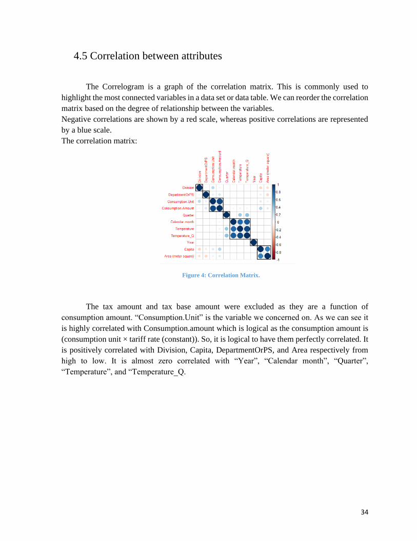
4.5 Correlation between attributes
The Correlogram is a graph of the correlation matrix. This is commonly used to
highlight the most connected variables in a data set or data table. We can reorder the correlation
matrix based on the degree of relationship between the variables.
Negative correlations are shown by a red scale, whereas positive correlations are represented
by a blue scale.
The correlation matrix:
Figure 4: Correlation Matrix.
The tax amount and tax base amount were excluded as they are a function of
consumption amount. “Consumption.Unit” is the variable we concerned on. As we can see it
is highly correlated with Consumption.amount which is logical as the consumption amount is
(consumption unit × tariff rate (constant)). So, it is logical to have them perfectly correlated. It
is positively correlated with Division, Capita, DepartmentOrPS, and Area respectively from
high to low. It is almost zero correlated with “Year”, “Calendar month”, “Quarter”,
“Temperature”, and “Temperature_Q.
35
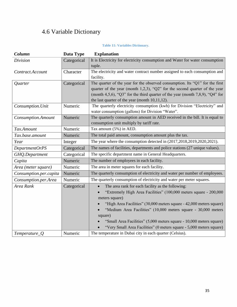
4.6 Variable Dictionary
Table 11: Variables Dictionary.
Column Data Type Explanation
Division Categorical It is Electricity for electricity consumption and Water for water consumption
tuple.
Contract.Account Character The electricity and water contract number assigned to each consumption and
facility.
Quarter Categorical The quarter of the year for the observed consumption. Its “Q1” for the first
quarter of the year (month 1,2,3), “Q2” for the second quarter of the year
(month 4,5,6), “Q3” for the third quarter of the year (month 7,8,9), “Q4” for
the last quarter of the year (month 10,11,12).
Consumption.Unit Numeric The quarterly electricity consumption (kwh) for Division “Electricity” and
water consumption (gallons) for Division “Water”.
Consumption.Amount Numeric The quarterly consumption amount in AED received in the bill. It is equal to
consumption unit multiply by tariff rate.
Tax.Amount Numeric Tax amount (5%) in AED.
Tax.base.amount Numeric The total paid amount, consumption amount plus the tax.
Year Integer The year where the consumption detected in (2017,2018,2019,2020,2021).
DepartmentOrPS Categorical The names of facilities, departments and police stations (27 unique values).
GHQ.Department Categorical The specific department name in General Headquarters.
Capita Numeric The number of employees in each facility.
Area (meter square) Numeric The area in meter squares for each facility.
Consumption.per.capita Numeric The quarterly consumption of electricity and water per number of employees.
Consumption.per.Area Numeric The quarterly consumption of electricity and water per meter squares.
Area Rank Categorical • The area rank for each facility as the following:
• “Extremely High Area Facilities” (100,000 meters square - 200,000
meters square)
• “High Area Facilities” (30,000 meters square - 42,000 meters square)
• “Medium Area Facilities” (10,000 meters square - 30,000 meters
square)
• “Small Area Facilities” (5,000 meters square - 10,000 meters square)
• “Very Small Area Facilities” (0 meters square - 5,000 meters square)
Temperature_Q Numeric The temperature in Dubai city in each quarter (Celsius).
36
1.7 Data Exploration and Visualization
In this section, a set of graphs have been drawn separately for electricity and water
consumption to understand the data better before moving toward the modeling part. The plots were
done using R Studio and Tableau. This plot is established to have an overview of what type of
questions/information we will try to explore in this section, following is a set of questions that are
devised in this case.
• Average consumption units by category overall.
• Total Consumption units by year for electricity and water.
• Month-wise comparison of consumption units for electricity and water.
• The quarter-wise trend of consumption for each year for both water and electricity.
• A trend of consumption units over the past few years.
• Consumption units by GHQ Department and DepartmentOrPS for both water and
electricity.
• Consumption per capita and Consumption per area plots.
• A comparison of consumption based on each area rank.
• A sample of quarterly report of one department showing the percentage of saving/loss.
• The temperature affects consumption.
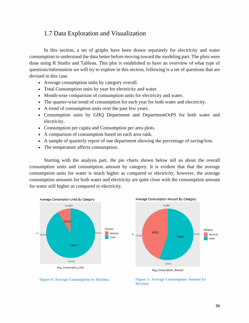
Starting with the analysis part, the pie charts shown below tell us about the overall
consumption units and consumption amount by category. It is evident that that the average
consumption units for water is much higher as compared to electricity, however, the average
consumption amounts for both water and electricity are quite close with the consumption amount
for water still higher as compared to electricity.
Figure 6: Average Consumption by Division. Figure 5: Average Consumption Amount by
Division.

37
The second plot attached below, shows the comparison of total consumption units by year
for both water and electricity. Figure 7, shows the consumption units by year for electricity while
Figure 8 shows the consumption units by year for water. We can see that the consumption units
for electricity are highest in year 2019 among all and lowest in year 2020. This might be due to
covid-19 pandemic where most of the departments were closed and employees working remotely
from home. Meanwhile the consumption for water is highest in year 2020 and lowest in year 2021.
The water consumption units are not affected by the covid-19 pandemic in this case.
Figure 7: Electricity Consumption by Year.
Figure 8: Water Consumption by Year.
Next, we will explore the total consumption units by month to see which month consumes
the highest units of electricity and water. We can see from below attached bar graphs that the
consumption units for electricity are recorded lowest in 2nd and 3rd month of each year respectively.
The highest consumption is recorded in 8th and 9th month which is August and September, the
peaks of summer season. Same trend is seen for water as well, the consumption is highest in 8th
month and lowest in 3rd month. This shows us that the time of year has a strong effect on
consumption of units.
Figure 9: Electriciy Consumption by Month.
Figure 10: Water Consumption by Month.
While looking at the quarter-wise comparison of consumption units for each year for
electricity, we can see that in almost all the years except 2019, the third quarter of the year records
the highest consumption of electricity. This information could be seen in the graphs attached
below:
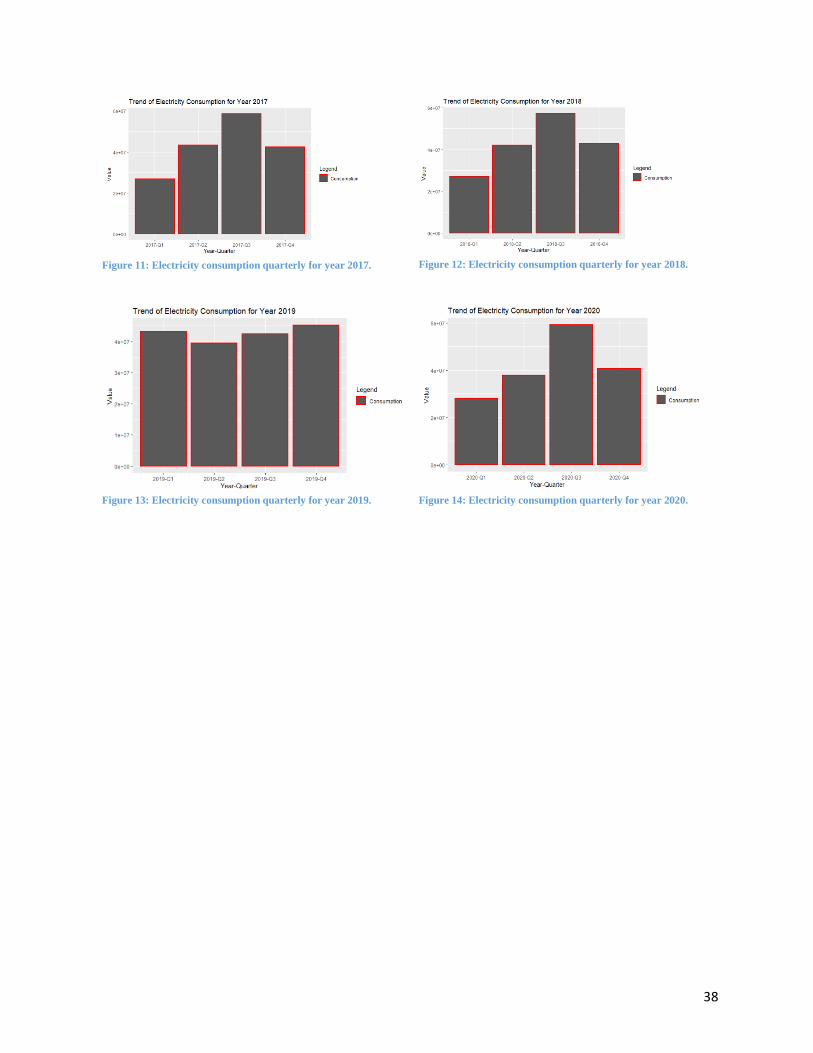
38
Figure 11: Electricity consumption quarterly for year 2017.
Figure 12: Electricity consumption quarterly for year 2018.
Figure 13: Electricity consumption quarterly for year 2019.
Figure 14: Electricity consumption quarterly for year 2020.

39
Same graphs are generated for water consumption as well and are attached below. Same
trend as observed above could be seen here as well except for year 2019. For 2019, the
consumptions are abrupt.
Figure 15: Water consumption quarterly for year 2017.
Figure 16: Water consumption quarterly for year 2018.
Figure 17: Water consumption quarterly for year 2019.
Figure 18: Water consumption quarterly for year 2020.
A graph showing the overall trend from 2017-2021 is attached below for both the
categories which are electricity and water consumption. From the trend for electricity
consumption, we can see that the lowest consumptions are recorded in first quarter of 2017 and
the highest is recorded in quarter 3rd of year 2020. Same for the consumption units of water, the
highest consumption for water is recorded in 1st quarter 2019 and lowest in 3rd quarter in 2019.

40
Figure 19: Electricity Consumption trend.
Figure 20: Water Consumption trend.

41
Below, two other bar graphs are created to show the department wise consumption for
water and electricity which are attached below. It can be seen that the consumption of electricity
for Forensic department and HQ building is highest while it is lowest for Decision making new
department. Similarly, the consumption of water is highest in GHQ shared and lowest in explosive
department.
Figure 21: Electricity Consumption for each GHQ Department.
Figure 22: Water Consumption for each GHQ Department.
In the below plots, the total electricity consumption per area and capita based on
departments or police stations for the total period of study (2017-2021) is shown. As we can see
the highest consumption per area is conducted for Al Faqqa Police Station and the lowest for Dubai
Police Academy. On the other hand, the highest consumption per capita was detected for Qusias
Warehouses and the lowest for Airport Security.
Figure 23: Electricity Consumption per Area for all departments
and PSs.
Figure 24: Electricity Consumption per Capita for all
departments and PSs.

42
Same for water consumption, as we can see the highest consumption per area is conducted
for Rawiyah Shooting Range, however the lowest for Al Riffa Police Station. In the other hand,
the highest consumption per capita was detected for Qusias Warehouses again and the lowest for
Airport Security, General Department of Transport and Rescue, and Lehbab Police Station.
Figure 25: Water Consumption per Area for all
departments and PSs.
Figure 26: Water Consumption per Capita for all
departments and PSs.
Moreover, the below plots showing electricity and water consumption for each department
based on their area ranks. For electricity plot, GHQ campus showed the highest consumption in
extremely high area facilities section, General Department of Transport and Rescue in high area
facilities, Officers Club in medium area facilities, Bur Dubai Police Station in small area facilities,
and Jabal Ali Police Station in very small area facilities. However, for water consumption Punitive
and Correctional Establishments showed the highest consumption in extremely high area facilities
section, Al Wasl Protective Security and Emergency in high area facilities, Traffic Department
Deira in medium area facilities, Airport Security in small area facilities, and Hor Al Anz Protective
Security and Emergency in very small area facilities. This concludes that these facilities need to
be focused on, to detect the reasons of their high consumptions compared with the other locations
in the same rank.
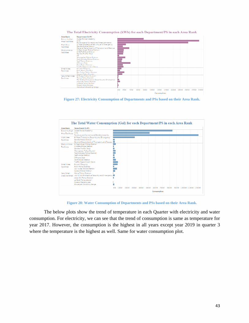
43
Figure 27: Electricity Consumption of Departments and PSs based on their Area Rank.
Figure 28: Water Consumption of Departments and PSs based on their Area Rank.
The below plots show the trend of temperature in each Quarter with electricity and water
consumption. For electricity, we can see that the trend of consumption is same as temperature for
year 2017. However, the consumption is the highest in all years except year 2019 in quarter 3
where the temperature is the highest as well. Same for water consumption plot.

44
Figure 29: The trend of temperature and electricity consumption each quarter.
Figure 30: The trend of temperature and water consumption each quarter.

45
The plots here show a sample for logical comparison per a specific Quarter (Q1) and a
facility (Al Riffa Police Station. In electricity consumption, first quarter of year 2019 got the
highest and 2021 got the lowest electricity consumption. In the other hand, for water consumption
in Q1, year 2020 detected the highest water consumption and 2018 the lowest.
Figure 31: A quarterly report of electricity consumption for Al Riffa PS for the first Quarter.
Figure 32: A quarterly report of water consumption for Al Riffa PS for the first Quarter.
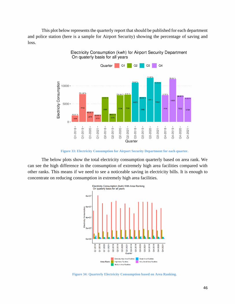
46
This plot below represents the quarterly report that should be published for each department
and police station (here is a sample for Airport Security) showing the percentage of saving and
loss.
Figure 33: Electricity Consumption for Airport Security Department for each quarter.
The below plots show the total electricity consumption quarterly based on area rank. We
can see the high difference in the consumption of extremely high area facilities compared with
other ranks. This means if we need to see a noticeable saving in electricity bills. It is enough to
concentrate on reducing consumption in extremely high area facilities.
Figure 34: Quarterly Electricity Consumption based on Area Ranking.
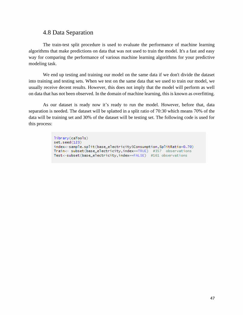
47
4.8 Data Separation
The train-test split procedure is used to evaluate the performance of machine learning
algorithms that make predictions on data that was not used to train the model. It's a fast and easy
way for comparing the performance of various machine learning algorithms for your predictive
modeling task.
We end up testing and training our model on the same data if we don't divide the dataset
into training and testing sets. When we test on the same data that we used to train our model, we
usually receive decent results. However, this does not imply that the model will perform as well
on data that has not been observed. In the domain of machine learning, this is known as overfitting.
As our dataset is ready now it’s ready to run the model. However, before that, data
separation is needed. The dataset will be splatted in a split ratio of 70:30 which means 70% of the
data will be training set and 30% of the dataset will be testing set. The following code is used for
this process:

48
4.9 Data Modeling
This project will study the dataset in Multiple linear regression model and ARIMA model.
The two models will be discussed based on the following performance evaluation metrics:
• ME:
The mean error (ME) is calculated by adding the variances and dividing the result by n.
Equation 1: Mean Error
𝑀𝐸 =𝑆𝑢𝑚 𝑜𝑓 𝐴𝑙𝑙 𝐸𝑟𝑟𝑜𝑟𝑠
𝑁𝑢𝑚𝑏𝑒𝑟 𝑜𝑓 𝑂𝑏𝑠𝑒𝑟𝑣𝑎𝑡𝑖𝑜𝑛𝑠
• RMSE:
The Root Mean Squared Error (RMSE) is an unusual measurement, but extremely useful
one. it is calculated by taking the square root of the average of summation of all squared error.
Equation 2: Root Mean Squared Error.
RMSE= √1
𝑛∑ 𝑒𝑡
2
• MAE:
The Mean Absolute Error (MAE) is an excellent metric for determining forecast accuracy.
It is calculated by finding the mean of the absolute error.
Equation 3: Mean Absolute Error.
MAE = 1
𝑛∑ |𝑒𝑡|
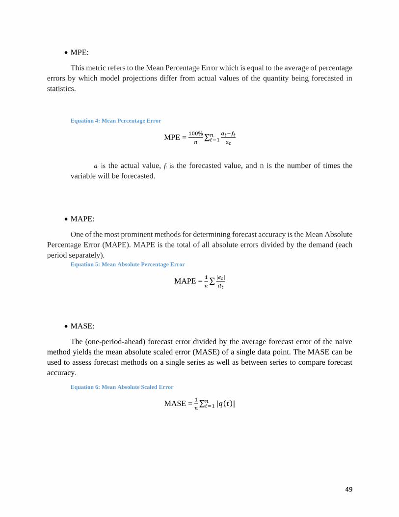
49
• MPE:
This metric refers to the Mean Percentage Error which is equal to the average of percentage
errors by which model projections differ from actual values of the quantity being forecasted in
statistics.
Equation 4: Mean Percentage Error
MPE = 100%
𝑛∑
𝑎𝑡−𝑓𝑡
𝑎𝑡
𝑛𝑡−1
at is the actual value, ft is the forecasted value, and n is the number of times the
variable will be forecasted.
• MAPE:
One of the most prominent methods for determining forecast accuracy is the Mean Absolute
Percentage Error (MAPE). MAPE is the total of all absolute errors divided by the demand (each
period separately). Equation 5: Mean Absolute Percentage Error
MAPE = 1
𝑛∑
|𝑒𝑡|
𝑑𝑡
• MASE:
The (one-period-ahead) forecast error divided by the average forecast error of the naive
method yields the mean absolute scaled error (MASE) of a single data point. The MASE can be
used to assess forecast methods on a single series as well as between series to compare forecast
accuracy.
Equation 6: Mean Absolute Scaled Error
MASE = 1
𝑛∑ |𝑞(𝑡)|𝑛
𝑡=1
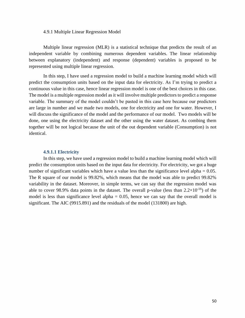
50
4.9.1 Multiple Linear Regression Model
Multiple linear regression (MLR) is a statistical technique that predicts the result of an
independent variable by combining numerous dependent variables. The linear relationship
between explanatory (independent) and response (dependent) variables is proposed to be
represented using multiple linear regression.
In this step, I have used a regression model to build a machine learning model which will
predict the consumption units based on the input data for electricity. As I’m trying to predict a
continuous value in this case, hence linear regression model is one of the best choices in this case.
The model is a multiple regression model as it will involve multiple predictors to predict a response
variable. The summary of the model couldn’t be pasted in this case here because our predictors
are large in number and we made two models, one for electricity and one for water. However, I
will discuss the significance of the model and the performance of our model. Two models will be
done, one using the electricity dataset and the other using the water dataset. As combing them
together will be not logical because the unit of the out dependent variable (Consumption) is not
identical.
4.9.1.1 Electricity
In this step, we have used a regression model to build a machine learning model which will
predict the consumption units based on the input data for electricity. For electricity, we got a huge
number of significant variables which have a value less than the significance level alpha = 0.05.
The R square of our model is 99.82%, which means that the model was able to predict 99.82%
variability in the dataset. Moreover, in simple terms, we can say that the regression model was
able to cover 98.9% data points in the dataset. The overall p-value (less than 2.2×10⁻¹⁶) of the
model is less than significance level alpha = 0.05, hence we can say that the overall model is
significant. The AIC (9915.891) and the residuals of the model (131800) are high.
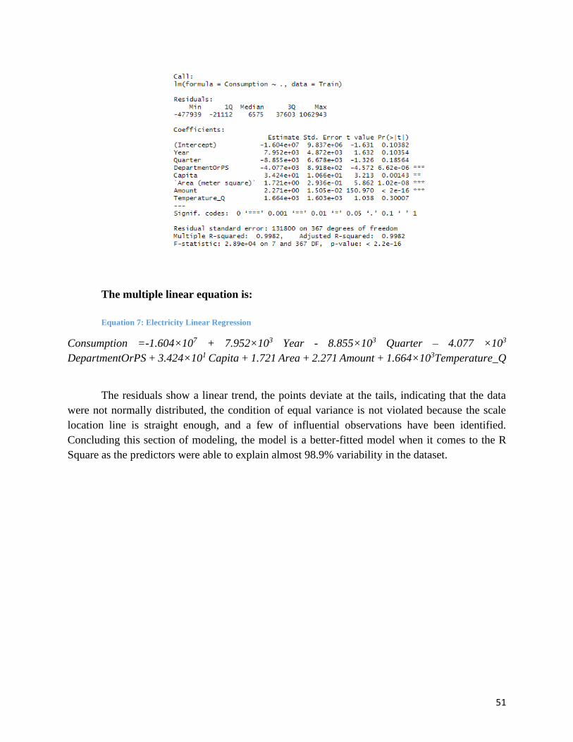
51
The multiple linear equation is:
Equation 7: Electricity Linear Regression
Consumption =-1.604×10⁷ + 7.952×10³ Year - 8.855×10³ Quarter – 4.077 ×10³
DepartmentOrPS + 3.424×101 Capita + 1.721 Area + 2.271 Amount + 1.664×10³Temperature_Q
The residuals show a linear trend, the points deviate at the tails, indicating that the data
were not normally distributed, the condition of equal variance is not violated because the scale
location line is straight enough, and a few of influential observations have been identified.
Concluding this section of modeling, the model is a better-fitted model when it comes to the R
Square as the predictors were able to explain almost 98.9% variability in the dataset.
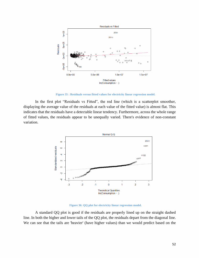
52
Figure 35 : Residuals versus fitted values for electricity linear regression model.
In the first plot “Residuals vs Fitted”, the red line (which is a scatterplot smoother,
displaying the average value of the residuals at each value of the fitted value) is almost flat. This
indicates that the residuals have a detectable linear tendency. Furthermore, across the whole range
of fitted values, the residuals appear to be unequally varied. There's evidence of non-constant
variation.
Figure 36: QQ plot for electricity linear regression model.
A standard QQ plot is good if the residuals are properly lined up on the straight dashed
line. In both the higher and lower tails of the QQ plot, the residuals depart from the diagonal line.
We can see that the tails are 'heavier' (have higher values) than we would predict based on the
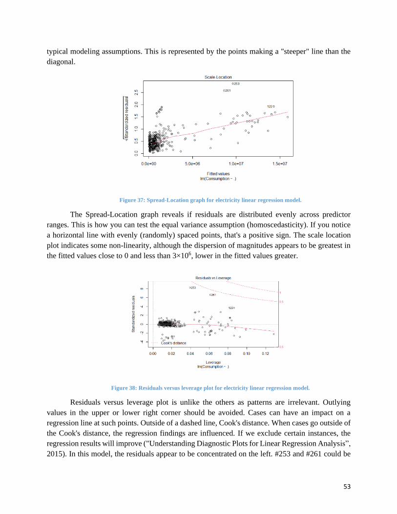
53
typical modeling assumptions. This is represented by the points making a "steeper" line than the
diagonal.
Figure 37: Spread-Location graph for electricity linear regression model.
The Spread-Location graph reveals if residuals are distributed evenly across predictor
ranges. This is how you can test the equal variance assumption (homoscedasticity). If you notice
a horizontal line with evenly (randomly) spaced points, that's a positive sign. The scale location
plot indicates some non-linearity, although the dispersion of magnitudes appears to be greatest in
the fitted values close to 0 and less than 3×10⁶, lower in the fitted values greater.
Figure 38: Residuals versus leverage plot for electricity linear regression model.
Residuals versus leverage plot is unlike the others as patterns are irrelevant. Outlying
values in the upper or lower right corner should be avoided. Cases can have an impact on a
regression line at such points. Outside of a dashed line, Cook's distance. When cases go outside of
the Cook's distance, the regression findings are influenced. If we exclude certain instances, the
regression results will improve ("Understanding Diagnostic Plots for Linear Regression Analysis”,
2015). In this model, the residuals appear to be concentrated on the left. #253 and #261 could be
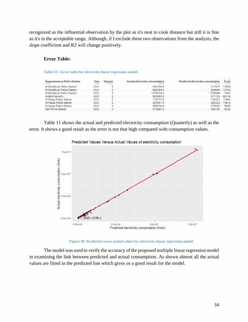
54
recognized as the influential observation by the plot as it's neat to cook distance but still it is fine
as it's in the acceptable range. Although, if I exclude these two observations from the analysis, the
slope coefficient and R2 will change positively.
Error Table:
Table 12 : Error table for electricity linear regression model.
Table 11 shows the actual and predicted electricity consumption (Quarterly) as well as the
error. It shows a good result as the error is not that high compared with consumption values.
Figure 39: Predicted versus actual values for electricity linear regression model.
The model was used to verify the accuracy of the proposed multiple linear regression model
in examining the link between predicted and actual consumption. As shown almost all the actual
values are fitted in the predicted line which gives us a good result for the model.

55
4.9.1.2 Water
The same was done for water consumption prediction, we got a huge number of significant
variables which have a value less than the significance level alpha = 0.05. The R square of our
model is 99.86%, which means that the model was able to predict 99.86% variability in the dataset.
Moreover, in simple terms, we can say that the regression model was able to cover 98.9% data
points in the dataset. The overall p-value (is less than 2.2×10⁻¹⁶) of the model is less than
significance level alpha = 0.05, hence we can say that the overall model is significant. The AIC
(10231.53) and the residuals of the model (554200) are high.
The multiple linear equation is:
Equation 8: Water Linear Regression
Consumption =-8.779×10⁷ + 4.344×10⁴ Year - 2.753×10⁴ Quarter + 9.413×10²
DepartmentOrPS + 1.307×10² Capita + 1.298 Area + 19.5 Amount + 4.058×10³ Temperature_Q

56
Figure 40: Residuals versus fitted values for water linear regression model.
We can see that residuals appear to be unequally varied as in electricity consumption.
There's evidence of non-constant variation.
Figure 41: QQ plot for water linear regression model.
We can see that the tails are 'heavier' than we would predict based on the typical modeling
assumptions. This is represented by the points making a "steeper" line than the diagonal.
Figure 42: Spread-Location graph for water linear regression model.

57
The scale location plot indicates non-linearity, although the dispersion of magnitudes
appears to be greatest in the lowest fitted values and almost nothing for higher values. As it shows
a steep angle which means it’s not horizontal at all.
Figure 43: Residuals versus leverage plot for water linear regression model.
In this model, the residuals appear to be concentrated from leverage 0.01 to almost 0.04
was recognized as an influential observation by the plot. Observation 241 is an outlying value in
this model.
Error Table:
Table 13: Error table for water linear regression model.
A table was built to show the (Quarterly) actual and predicted water consumption as well
as the error. A sample of the water consumption data is presented in Table 13. It doesn’t show bad
results as the error is not that high compared with consumption values.

58
Figure 44: Predicted versus actual values for water linear regression model.
Here as well it showed almost all the actual water consumption values are fitted in the
predicted line which gives us a good result for the model.
4.9.1.4 Accuracy Table Table 14: Accuracy Table for electricity and water models.
The accuracy parameters was calculated using accuracy() function in R for both models
based on the test dataset. The table above shows a summary of the two models results of the six
measurements. I will discuss here the RMSE and MAPE values. For the electricity regression
model the RMSE and MAPE are 130385.3 kWh and 11.89% respectively. In the other hand, for
the water model they are equal to 547776.9 Gallons and 9.53% respectively. both models gave us
a good result.
All of these outputs provide information about your model and data. The existing model
may not be the most effective approach to comprehend the information we have. That’s why I
build a time series model to check if we will get a better result.
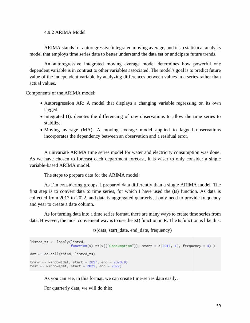
59
4.9.2 ARIMA Model
ARIMA stands for autoregressive integrated moving average, and it's a statistical analysis
model that employs time series data to better understand the data set or anticipate future trends.
An autoregressive integrated moving average model determines how powerful one
dependent variable is in contrast to other variables associated. The model's goal is to predict future
value of the independent variable by analyzing differences between values in a series rather than
actual values.
Components of the ARIMA model:
• Autoregression AR: A model that displays a changing variable regressing on its own
lagged.
• Integrated (I): denotes the differencing of raw observations to allow the time series to
stabilize.
• Moving average (MA): A moving average model applied to lagged observations
incorporates the dependency between an observation and a residual error.
A univariate ARIMA time series model for water and electricity consumption was done.
As we have chosen to forecast each department forecast, it is wiser to only consider a single
variable-based ARIMA model.
The steps to prepare data for the ARIMA model:
As I’m considering groups, I prepared data differently than a single ARIMA model. The
first step is to convert data to time series, for which I have used the (ts) function. As data is
collected from 2017 to 2022, and data is aggregated quarterly, I only need to provide frequency
and year to create a date column.
As for turning data into a time series format, there are many ways to create time series from
data. However, the most convenient way is to use the ts() function in R. The ts function is like this:
ts(data, start_date, end_date, frequency)
As you can see, in this format, we can create time-series data easily.
For quarterly data, we will do this:
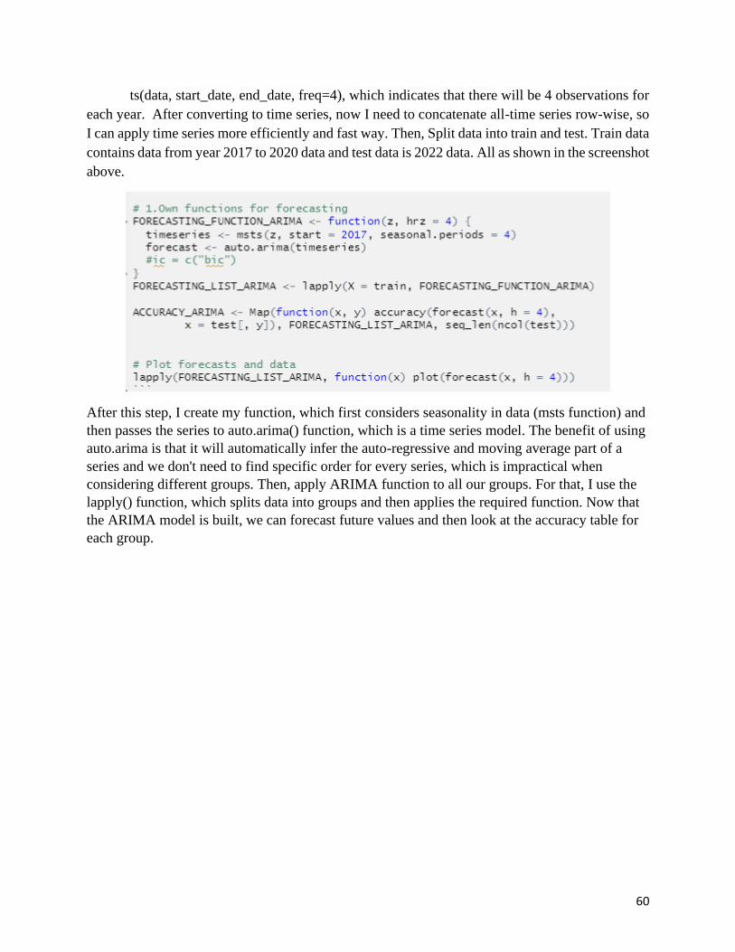
60
ts(data, start_date, end_date, freq=4), which indicates that there will be 4 observations for
each year. After converting to time series, now I need to concatenate all-time series row-wise, so
I can apply time series more efficiently and fast way. Then, Split data into train and test. Train data
contains data from year 2017 to 2020 data and test data is 2022 data. All as shown in the screenshot
above.
After this step, I create my function, which first considers seasonality in data (msts function) and
then passes the series to auto.arima() function, which is a time series model. The benefit of using
auto.arima is that it will automatically infer the auto-regressive and moving average part of a
series and we don't need to find specific order for every series, which is impractical when
considering different groups. Then, apply ARIMA function to all our groups. For that, I use the
lapply() function, which splits data into groups and then applies the required function. Now that
the ARIMA model is built, we can forecast future values and then look at the accuracy table for
each group.
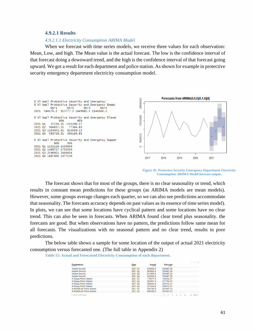
61
4.9.2.1 Results
4.9.2.1.1 Electricity Consumption ARIMA Model
When we forecast with time series models, we receive three values for each observation:
Mean, Low, and high. The Mean value is the actual forecast. The low is the confidence interval of
that forecast doing a downward trend, and the high is the confidence interval of that forecast going
upward. We got a result for each department and police station. As shown for example in protective
security emergency department electricity consumption model.
The forecast shows that for most of the groups, there is no clear seasonality or trend, which
results in constant mean predictions for these groups (as ARIMA models are mean models).
However, some groups average changes each quarter, so we can also see predictions accommodate
that seasonality. The forecasts accuracy depends on past values as its essence of time series model).
In plots, we can see that some locations have cyclical pattern and some locations have no clear
trend. This can also be seen in forecasts. When ARIMA found clear trend plus seasonality. the
forecasts are good. But when observations have no pattern, the predictions follow same mean for
all forecasts. The visualizations with no seasonal pattern and no clear trend, results in poor
predictions.
The below table shows a sample for some location of the output of actual 2021 electricity
consumption versus forecasted one. (The full table in Appendix 2)
Table 15: Actual and Forecasted Electricity Consumption of each department.
Figure 45: Protective Security Emergency Department Electricity
Consumption ARIMA Model forecast output.
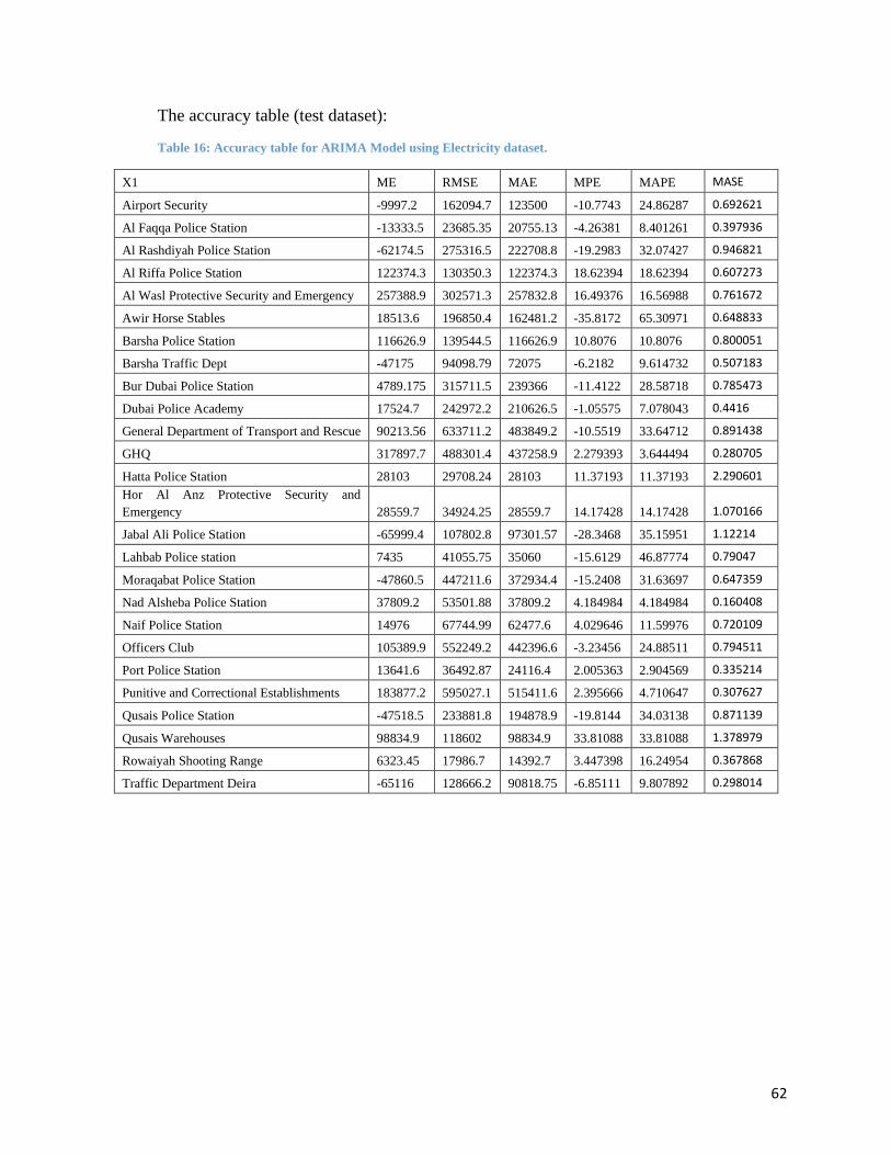
62
The accuracy table (test dataset):
Table 16: Accuracy table for ARIMA Model using Electricity dataset.
X1 ME RMSE MAE MPE MAPE MASE
Airport Security -9997.2 162094.7 123500 -10.7743 24.86287 0.692621
Al Faqqa Police Station -13333.5 23685.35 20755.13 -4.26381 8.401261 0.397936
Al Rashdiyah Police Station -62174.5 275316.5 222708.8 -19.2983 32.07427 0.946821
Al Riffa Police Station 122374.3 130350.3 122374.3 18.62394 18.62394 0.607273
Al Wasl Protective Security and Emergency 257388.9 302571.3 257832.8 16.49376 16.56988 0.761672
Awir Horse Stables 18513.6 196850.4 162481.2 -35.8172 65.30971 0.648833
Barsha Police Station 116626.9 139544.5 116626.9 10.8076 10.8076 0.800051
Barsha Traffic Dept -47175 94098.79 72075 -6.2182 9.614732 0.507183
Bur Dubai Police Station 4789.175 315711.5 239366 -11.4122 28.58718 0.785473
Dubai Police Academy 17524.7 242972.2 210626.5 -1.05575 7.078043 0.4416
General Department of Transport and Rescue 90213.56 633711.2 483849.2 -10.5519 33.64712 0.891438
GHQ 317897.7 488301.4 437258.9 2.279393 3.644494 0.280705
Hatta Police Station 28103 29708.24 28103 11.37193 11.37193 2.290601
Hor Al Anz Protective Security and
Emergency 28559.7 34924.25 28559.7 14.17428 14.17428 1.070166
Jabal Ali Police Station -65999.4 107802.8 97301.57 -28.3468 35.15951 1.12214
Lahbab Police station 7435 41055.75 35060 -15.6129 46.87774 0.79047
Moraqabat Police Station -47860.5 447211.6 372934.4 -15.2408 31.63697 0.647359
Nad Alsheba Police Station 37809.2 53501.88 37809.2 4.184984 4.184984 0.160408
Naif Police Station 14976 67744.99 62477.6 4.029646 11.59976 0.720109
Officers Club 105389.9 552249.2 442396.6 -3.23456 24.88511 0.794511
Port Police Station 13641.6 36492.87 24116.4 2.005363 2.904569 0.335214
Punitive and Correctional Establishments 183877.2 595027.1 515411.6 2.395666 4.710647 0.307627
Qusais Police Station -47518.5 233881.8 194878.9 -19.8144 34.03138 0.871139
Qusais Warehouses 98834.9 118602 98834.9 33.81088 33.81088 1.378979
Rowaiyah Shooting Range 6323.45 17986.7 14392.7 3.447398 16.24954 0.367868
Traffic Department Deira -65116 128666.2 90818.75 -6.85111 9.807892 0.298014
63
I will discuss 3 Metrics which are considered standard: MSE, RMSE, and MAPE. The
metrics are difference between actual and predicted values in terms of Mean Square Error and
Mean percentage error (MAPE).
If I take Al Faqqa Police Station as example (Electricity consumption prediction)
ME RMSE MAE MPE MAPE MASE ACF1 Theil's U
Training set 22.76526 54413.77 38256.25 -8.627517 22.754437 0.7334835 0.2834065 NA
Test set -13333.46667 23685.35 20755.13 -4.263807 8.401261 0.3979362 0.2586741 0.1957359
The RMSE metrics shows that for training set, error margin was 54413.77 units
(predictions can be off with this difference (+/-), and for test set, this metric is 23685.35 which is
much better.
Same is true for MSE, which is similar to RMSE. As for MAPE it shows percentage
difference between predictions and actual values. In this case the training set has larger MAPE
(22.75) than test set (8.4).
So, it means that predictions are not that bad this will be considered small error margin.
Some will be larger and others will be even smaller than this. The actual and prediction values was
shown in previous section. The average MAPE calculated for all location in the model to be 20.02.
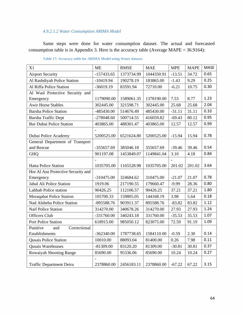
64
4.9.2.1.2 Water Consumption ARIMA Model
Same steps were done for water consumption dataset. The actual and forecasted
consumption table is in Appendix 3. Here is the accuracy table (Average MAPE = 36.9164):
Table 17: Accuracy table for ARIMA Model using Water dataset.
X1 ME RMSE MAE MPE MAPE MASE
Airport Security -157433.65 1373734.99 1044350.91 -13.51 34.72 0.65
Al Rashdiyah Police Station -10419.94 190278.19 183865.00 -1.43 9.29 0.25
Al Riffa Police Station -36019.19 83591.94 72710.00 -6.21 10.75 0.30
Al Wasl Protective Security and
Emergency 1179090.00 1589061.35 1378190.00 7.53 8.77 1.23
Awir Horse Stables 302445.00 321598.71 302445.00 25.68 25.68 2.04
Barsha Police Station -485430.00 514676.49 485430.00 -31.11 31.11 0.33
Barsha Traffic Dept -278048.60 500714.55 416059.82 -69.43 80.12 0.95
Bur Dubai Police Station 403865.00 488301.47 403865.00 12.57 12.57 0.99
Dubai Police Academy
-
5200525.00 6521624.80 5200525.00 -15.94 15.94 0.78
General Department of Transport
and Rescue -355657.69 385046.18 355657.69 -39.46 39.46 0.54
GHQ 901197.08 1453849.07 1149841.04 3.10 4.18 0.84
Hatta Police Station
-
1035705.00 1165528.98 1035705.00
-
201.02 201.02 3.64
Hor Al Anz Protective Security and
Emergency -310475.00 324684.62 310475.00 -21.07 21.07 0.78
Jabal Ali Police Station 1919.06 217190.55 179660.47 -9.99 28.36 0.80
Lahbab Police station 90426.25 112106.57 90426.25 37.21 37.21 1.80
Moraqabat Police Station 105700.33 159805.05 144168.19 3.98 5.64 0.18
Nad Alsheba Police Station -895588.76 903911.37 895588.76 -83.82 83.82 1.12
Naif Police Station 314270.00 340678.26 314270.00 27.93 27.93 1.24
Officers Club -331760.00 340243.18 331760.00 -35.53 35.53 1.07
Port Police Station 618915.00 985050.12 823075.00 72.59 91.19 1.09
Punitive and Correctional
Establishments -362340.00 1787738.65 1584110.00 -0.59 2.30 0.14
Qusais Police Station 10010.00 88093.04 81400.00 0.26 7.98 0.11
Qusais Warehouses -81309.00 83120.20 81309.00 -30.81 30.81 0.37
Rowaiyah Shooting Range 85690.00 95336.06 85690.00 10.24 10.24 0.27
Traffic Department Deira
-
2378860.00 2456183.11 2378860.00 -67.22 67.22 3.15
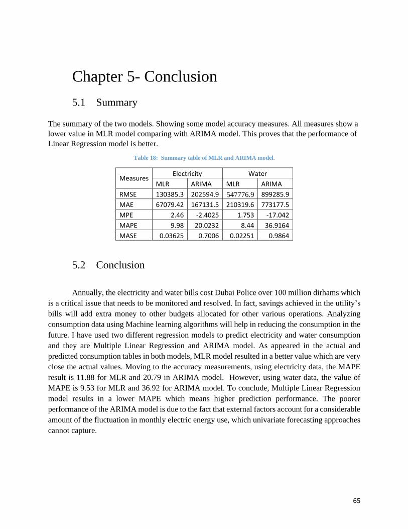
65
Chapter 5- Conclusion
5.1 Summary
The summary of the two models. Showing some model accuracy measures. All measures show a
lower value in MLR model comparing with ARIMA model. This proves that the performance of
Linear Regression model is better.
Table 18: Summary table of MLR and ARIMA model.
Measures Electricity Water
MLR ARIMA MLR ARIMA
RMSE 130385.3 202594.9 547776.9 899285.9
MAE 67079.42 167131.5 210319.6 773177.5
MPE 2.46 -2.4025 1.753 -17.042
MAPE 9.98 20.0232 8.44 36.9164
MASE 0.03625 0.7006 0.02251 0.9864
5.2 Conclusion
Annually, the electricity and water bills cost Dubai Police over 100 million dirhams which
is a critical issue that needs to be monitored and resolved. In fact, savings achieved in the utility’s
bills will add extra money to other budgets allocated for other various operations. Analyzing
consumption data using Machine learning algorithms will help in reducing the consumption in the
future. I have used two different regression models to predict electricity and water consumption
and they are Multiple Linear Regression and ARIMA model. As appeared in the actual and
predicted consumption tables in both models, MLR model resulted in a better value which are very
close the actual values. Moving to the accuracy measurements, using electricity data, the MAPE
result is 11.88 for MLR and 20.79 in ARIMA model. However, using water data, the value of
MAPE is 9.53 for MLR and 36.92 for ARIMA model. To conclude, Multiple Linear Regression
model results in a lower MAPE which means higher prediction performance. The poorer
performance of the ARIMA model is due to the fact that external factors account for a considerable
amount of the fluctuation in monthly electric energy use, which univariate forecasting approaches
cannot capture.
66
5.3 Recommendations
This study can be used by Dubai Police, specifically the energy conservation department,
to place remedial measures to reduce the consumption of the highest consuming facilities that have
been identified. In addition, factoring in the temperature parameter in the model, Dubai Police
should focus on spreading more awareness with regards to the consumer behavior during the
summer season as the consumption peaks. Finally, this study findings can facilitate a baseline for
Dubai Police to adopt clean solar energy into its facilities, starting with the highest consuming
facilities.
5.4 Future Works
Although for this research work the dataset was somehow limited due to confidentiality
reasons as stated earlier, being an employee at the energy conservation department in Dubai Police,
I will be able to access the full dataset and make a detailed study containing all operational, capita,
and area data. As well as, to add a multivariant ARIMA model to the study and compare it with
the existing models.
67
References
1. Understanding Diagnostic Plots for Linear Regression Analysis | University of Virginia Library
Research Data Services + Sciences. (2015). Retrieved 20 April 2022.
2. Amasyali, K. and El-Gohary, N., 2018. A review of data-driven building energy consumption
prediction studies. Renewable and Sustainable Energy Reviews, 81, pp.1192-1205.
3. Nafil, A., Bouzi, M., Anoune, K. and Ettalabi, N., 2020. Comparative study of forecasting
methods for energy demand in Morocco. Energy Reports, 6, pp.523-536.
4. Singh, S. and Yassine, A., 2018. Big Data Mining of Energy Time Series for Behavioral
Analytics and Energy Consumption Forecasting. Energies, 11(2), p.452.
5. Yang, J., Ning, C., Deb, C., Zhang, F., Cheong, D., Lee, S., Sekhar, C. and Tham, K., 2017. k-
Shape clustering algorithm for building energy usage patterns analysis and forecasting model accuracy
improvement. Energy and Buildings, 146, pp.27-37.
6. Aranda, A., Ferreira, G., Mainar-Toledo, M., Scarpellini, S. and Llera Sastresa, E., 2012.
Multiple regression models to predict the annual energy consumption in the Spanish banking sector. Energy
and Buildings, 49, pp.380-387.
7. Tso, G. and Yau, K., 2007. Predicting electricity energy consumption: A comparison of
regression analysis, decision tree and neural networks. Energy, 32(9), pp.1761-1768.
8. Banihashemi, S., Ding, G. and Wang, J., 2017. Developing a Hybrid Model of Prediction and
Classification Algorithms for Building Energy Consumption. Energy Procedia, 110, pp.371-376.
9. Jamii, M. and Maaroufi, M., 2021. The Forecasting of Electrical Energy Consumption in
Morocco with an Autoregressive Integrated Moving Average Approach. Mathematical Problems in
Engineering, 2021, pp.1-9.
10. Wang, X. and Meng, M., 2012. A Hybrid Neural Network and ARIMA Model for Energy
Consumption Forcasting. Journal of Computers, 7(5).
11. Sen, P., Roy, M. and Pal, P., 2016. Application of ARIMA for forecasting energy consumption
and GHG emission: A case study of an Indian pig iron manufacturing organization. Energy, 116, pp.1031-
1038.
12. Pérez-Chacón, R., Luna-Romera, J., Troncoso, A., Martínez-Álvarez, F. and Riquelme, J.,
2018. Big Data Analytics for Discovering Electricity Consumption Patterns in Smart Cities. Energies,
11(3), p.683.
13. Yuan, C., Liu, S. and Fang, Z., 2016. Comparison of China's primary energy consumption
forecasting by using ARIMA (the autoregressive integrated moving average) model and GM(1,1)
model. Energy, 100, pp.384-390.
68
14. Liu, Y., Chen, H., Zhang, L., Wu, X. and Wang, X., 2020. Energy consumption prediction and
diagnosis of public buildings based on support vector machine learning: A case study in China. Journal of
Cleaner Production, 272, p.122542.
15. Shapi, M., Ramli, N. and Awalin, L., 2021. Energy consumption prediction by using machine
learning for smart building: Case study in Malaysia. Developments in the Built Environment, 5, p.100037.
16. Zhao, H. and Magoulès, F., 2012. Feature Selection for Predicting Building Energy
Consumption Based on Statistical Learning Method. Journal of Algorithms & Computational
Technology, 6(1), pp.59-77.
17. de Oliveira, E. and Cyrino Oliveira, F., 2018. Forecasting mid-long term electric energy
consumption through bagging ARIMA and exponential smoothing methods. Energy, 144, pp.776-788.
18. Carrera, B., Peyrard, S. and Kim, K., 2021. Meta-regression framework for energy consumption
prediction in a smart city: A case study of Songdo in South Korea. Sustainable Cities and Society, 72,
p.103025.
19. Fumo, N. and Rafe Biswas, M., 2015. Regression analysis for prediction of residential energy
consumption. Renewable and Sustainable Energy Reviews, 47, pp.332-343.
20. Wang, X., 2022. Research on the prediction of per capita coal consumption based on the
ARIMA–BP combined model. Energy Reports, 8, pp.285-294.
21. Barak, S. and Sadegh, S., 2016. Forecasting energy consumption using ensemble ARIMA–
ANFIS hybrid algorithm. International Journal of Electrical Power & Energy Systems, 82, pp.92-104.
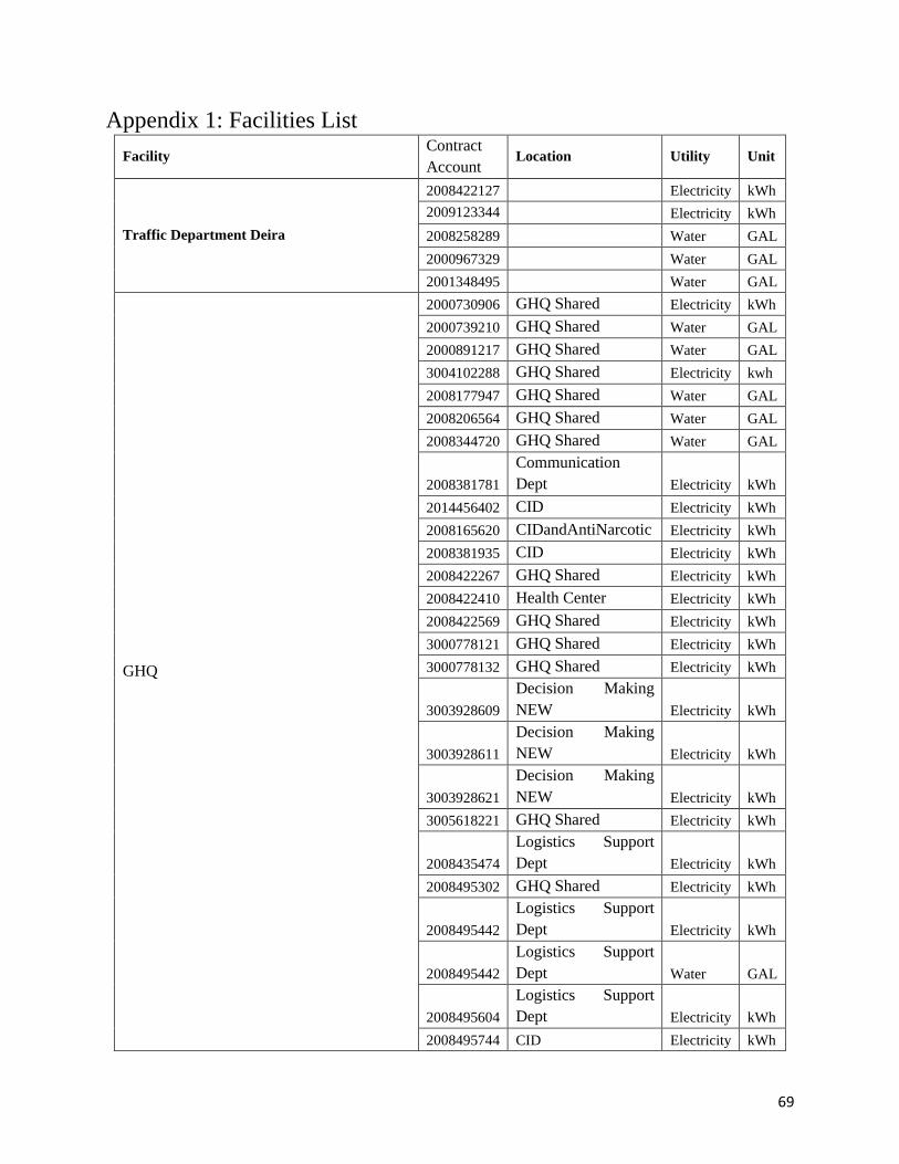
69
Appendix 1: Facilities List
Facility Contract
Account Location Utility Unit
Traffic Department Deira
2008422127 Electricity kWh
2009123344 Electricity kWh
2008258289 Water GAL
2000967329 Water GAL
2001348495 Water GAL
GHQ
2000730906 GHQ Shared Electricity kWh
2000739210 GHQ Shared Water GAL
2000891217 GHQ Shared Water GAL
3004102288 GHQ Shared Electricity kwh
2008177947 GHQ Shared Water GAL
2008206564 GHQ Shared Water GAL
2008344720 GHQ Shared Water GAL
2008381781
Communication
Dept Electricity kWh
2014456402 CID Electricity kWh
2008165620 CIDandAntiNarcotic Electricity kWh
2008381935 CID Electricity kWh
2008422267 GHQ Shared Electricity kWh
2008422410 Health Center Electricity kWh
2008422569 GHQ Shared Electricity kWh
3000778121 GHQ Shared Electricity kWh
3000778132 GHQ Shared Electricity kWh
3003928609
Decision Making
NEW Electricity kWh
3003928611
Decision Making
NEW Electricity kWh
3003928621
Decision Making
NEW Electricity kWh
3005618221 GHQ Shared Electricity kWh
2008435474
Logistics Support
Dept Electricity kWh
2008495302 GHQ Shared Electricity kWh
2008495442
Logistics Support
Dept Electricity kWh
2008495442
Logistics Support
Dept Water GAL
2008495604
Logistics Support
Dept Electricity kWh
2008495744 CID Electricity kWh

70
2008534081 GHQ Shared Water GAL
2009491912 GHQ Shared Electricity kWh
2009816927 Health Center Electricity kWh
2009816960
Communication
Dept Electricity kWh
2009943856 AntiNarcotic Electricity kWh
2010094239 HQ BLDG Electricity kWh
2010094980 HQ BLDG Electricity kWh
2010097041 HQ BLDG Electricity kWh
2010097106 HQ BLDG Electricity kWh
2010097130 HQ BLDG Electricity kWh
2010097181 HQ BLDG Electricity kWh
2010097211 HQ BLDG Electricity kWh
2010097246 HQ BLDG Electricity kWh
2010097300 HQ BLDG Electricity kWh
2014956103 GHQ Shared Electricity kWh
2016164379 GHQ Shared Water GAL
2016589701 Exsplosive Dept Electricity kWh
2016589701 Exsplosive Dept Water GAL
3000520413 Forensic Dept Electricity kWh
3000520424 Forensic Dept Electricity kWh
3000520435 Forensic Dept Electricity kWh
3000520446 Forensic Dept Electricity kWh
3000520457 Forensic Dept Electricity kWh
3000520468 Forensic Dept Electricity kWh
3000520479 Forensic Dept Electricity kWh
3000520481 Forensic Dept Electricity kWh
3000841131 Forensic Dept Water GAL
Airport Security 2008350827 Water GAL
2009043529 Electricity kWh
Punitive and Correctional Establishments
2008525686 Water GAL
2009912039 Electricity kWh
2009922859 Electricity kWh
2009922883 Electricity kWh
2009926587 Electricity kWh
2009960246 Electricity kWh
2009964810 Electricity kWh
2009964845 Electricity kWh
2009969537 Electricity kWh
2009969561 Electricity kWh
2009969596 Electricity kWh

71
2009969626 Electricity kWh
2009977513 Electricity kWh
2010034074 Electricity kWh
3000268799 Electricity kWh
3000268799 Water GAL
3000598481 Electricity kWh
3000613331 Electricity kWh
Awir Horse Stables
2020372649 Water GAL
3006065337 Electricity kWh
2020372657 Electricity kWh
Rowaiyah Shooting Range
2008465942 Electricity kWh
2009816323 Electricity kWh
2008541681 Water GAL
General Department of Transport and
Rescue
2008849929 Water GAL
2010331281 Electricity kWh
2010331303 Electricity kWh
2010331320 Electricity kWh
2010331354 Electricity kWh
2015925570 Electricity kWh
2015925589 Electricity kWh
2016979267 Electricity kWh
2016979275 Electricity kWh
Dubai Police Academy
2002192219 Water GAL
2002255792 Water GAL
2002255881 Water GAL
2008195619 Water GAL
2008234835 Water GAL
2008277623 Water GAL
2008399818 Electricity kWh
2008408388 Electricity kWh
2008413853 Electricity kWh
2008644553 Electricity kWh
2008644693 Electricity kWh
2008644839 Electricity kWh
2008686493 Electricity kWh
2008791459 Electricity kWh
2008798160 Electricity kWh
2008822273 Electricity kWh
2009465857 Electricity kWh
2009700015 Electricity kWh
2009787056 Electricity kWh

72
2009811755 Electricity kWh
Barsha Police Station
2015841393 Water GAL
2015841393 Electricity kWh
2015841407 Electricity kWh
Barsha Traffic Dept 2008453243 Water GAL
2008640302 Electricity kWh
Bur Dubai Police Station
2008280187 Water GAL
2008359280 Electricity kWh
2008359352 Electricity kWh
2008613607 Electricity kWh
2001927282 Electricity kWh
Officers Club
2008325393 Electricity kWh
2008334333 Water GAL
2008325466 Electricity kWh
2009577922 Electricity kWh
Al Faqqa Police Station
2000573312 Electricity kWh
3002582616 Electricity kWh
2002028230 Electricity kWh
Hatta Police Station
2000297099 Electricity kWh
2000297099 Water GAL
2000297170 Electricity kWh
2000297170 Water GAL
2000297250 Water GAL
2003410686 Electricity kWh
Jabal Ali Police Station
3000073472 Electricity kWh
3000073483 Electricity kWh
3000229001 Water GAL
Lahbab Police station 2000674720 Electricity kWh
2016240032 Water GAL
Moraqabat Police Station
2005947121 Electricity kWh
2005947253 Electricity kWh
2006241800 Electricity kWh
2006241800 Water GAL
2008507050 Water GAL
Nad Alsheba Police Station
2001125488 Water GAL
2008450660 Electricity kWh
2008456072 Electricity kWh
2008456927 Electricity kWh
Naif Police Station
2001467010 Water GAL
2004124580 Electricity kWh
2015722335 Electricity kWh
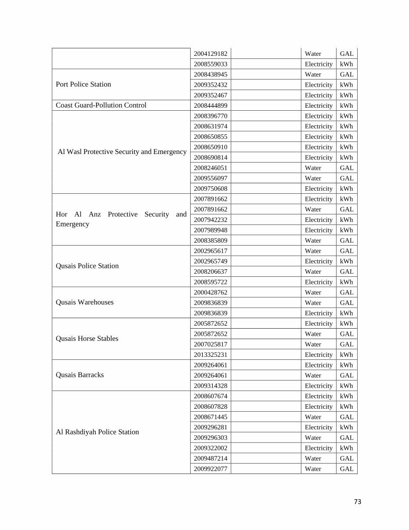
73
2004129182 Water GAL
2008559033 Electricity kWh
Port Police Station
2008438945 Water GAL
2009352432 Electricity kWh
2009352467 Electricity kWh
Coast Guard-Pollution Control 2008444899 Electricity kWh
Al Wasl Protective Security and Emergency
2008396770 Electricity kWh
2008631974 Electricity kWh
2008650855 Electricity kWh
2008650910 Electricity kWh
2008690814 Electricity kWh
2008246051 Water GAL
2009556097 Water GAL
2009750608 Electricity kWh
Hor Al Anz Protective Security and
Emergency
2007891662 Electricity kWh
2007891662 Water GAL
2007942232 Electricity kWh
2007989948 Electricity kWh
2008385809 Water GAL
Qusais Police Station
2002965617 Water GAL
2002965749 Electricity kWh
2008206637 Water GAL
2008595722 Electricity kWh
Qusais Warehouses
2000428762 Water GAL
2009836839 Water GAL
2009836839 Electricity kWh
Qusais Horse Stables
2005872652 Electricity kWh
2005872652 Water GAL
2007025817 Water GAL
2013325231 Electricity kWh
Qusais Barracks
2009264061 Electricity kWh
2009264061 Water GAL
2009314328 Electricity kWh
Al Rashdiyah Police Station
2008607674 Electricity kWh
2008607828 Electricity kWh
2008671445 Water GAL
2009296281 Electricity kWh
2009296303 Water GAL
2009322002 Electricity kWh
2009487214 Water GAL
2009922077 Water GAL

74
2010002610 Electricity kWh
Al Riffa Police Station
2008892646 Electricity kWh
2008892875 Electricity kWh
2009055420 Water GAL
2009222180 Electricity kWh
K9 3003551419 Electricity kWh
Bur Dubai Detention
3004123782 Electricity kWh
3004123771 Electricity kWh
3004123771 Water GAL
Lost and Found department 3006175414 Electricity kWh
Water GAL
Al Khawaneej Police Station 3004604086 Electricity kWh
3004604086 Water GAL
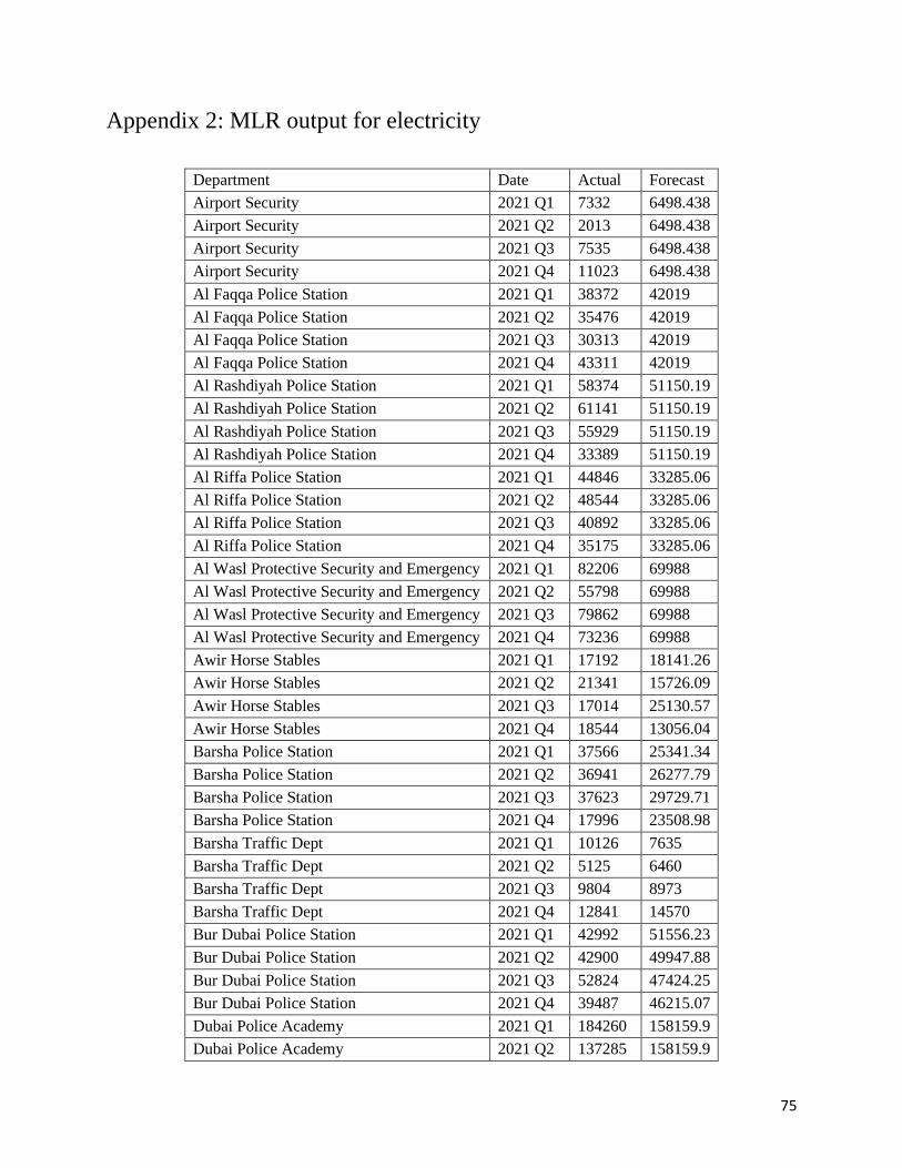
75
Appendix 2: MLR output for electricity
Department Date Actual Forecast
Airport Security 2021 Q1 7332 6498.438
Airport Security 2021 Q2 2013 6498.438
Airport Security 2021 Q3 7535 6498.438
Airport Security 2021 Q4 11023 6498.438
Al Faqqa Police Station 2021 Q1 38372 42019
Al Faqqa Police Station 2021 Q2 35476 42019
Al Faqqa Police Station 2021 Q3 30313 42019
Al Faqqa Police Station 2021 Q4 43311 42019
Al Rashdiyah Police Station 2021 Q1 58374 51150.19
Al Rashdiyah Police Station 2021 Q2 61141 51150.19
Al Rashdiyah Police Station 2021 Q3 55929 51150.19
Al Rashdiyah Police Station 2021 Q4 33389 51150.19
Al Riffa Police Station 2021 Q1 44846 33285.06
Al Riffa Police Station 2021 Q2 48544 33285.06
Al Riffa Police Station 2021 Q3 40892 33285.06
Al Riffa Police Station 2021 Q4 35175 33285.06
Al Wasl Protective Security and Emergency 2021 Q1 82206 69988
Al Wasl Protective Security and Emergency 2021 Q2 55798 69988
Al Wasl Protective Security and Emergency 2021 Q3 79862 69988
Al Wasl Protective Security and Emergency 2021 Q4 73236 69988
Awir Horse Stables 2021 Q1 17192 18141.26
Awir Horse Stables 2021 Q2 21341 15726.09
Awir Horse Stables 2021 Q3 17014 25130.57
Awir Horse Stables 2021 Q4 18544 13056.04
Barsha Police Station 2021 Q1 37566 25341.34
Barsha Police Station 2021 Q2 36941 26277.79
Barsha Police Station 2021 Q3 37623 29729.71
Barsha Police Station 2021 Q4 17996 23508.98
Barsha Traffic Dept 2021 Q1 10126 7635
Barsha Traffic Dept 2021 Q2 5125 6460
Barsha Traffic Dept 2021 Q3 9804 8973
Barsha Traffic Dept 2021 Q4 12841 14570
Bur Dubai Police Station 2021 Q1 42992 51556.23
Bur Dubai Police Station 2021 Q2 42900 49947.88
Bur Dubai Police Station 2021 Q3 52824 47424.25
Bur Dubai Police Station 2021 Q4 39487 46215.07
Dubai Police Academy 2021 Q1 184260 158159.9
Dubai Police Academy 2021 Q2 137285 158159.9

76
Dubai Police Academy 2021 Q3 182045 158159.9
Dubai Police Academy 2021 Q4 168054 158159.9
General Department of Transport and
Rescue 2021 Q1 114615 98841.5
General Department of Transport and
Rescue 2021 Q2 117698 98841.5
General Department of Transport and
Rescue 2021 Q3 102168 98841.5
General Department of Transport and
Rescue 2021 Q4 71957 98841.5
GHQ 2021 Q1 593584 521511.4
GHQ 2021 Q2 713147 521511.4
GHQ 2021 Q3 575332 521511.4
GHQ 2021 Q4 498503 521511.4
Hatta Police Station 2021 Q1 47811 53819
Hatta Police Station 2021 Q2 31863 27681
Hatta Police Station 2021 Q3 66683 65613
Hatta Police Station 2021 Q4 80847 80451
Hor Al Anz Protective Security and
Emergency 2021 Q1 53294 58767
Hor Al Anz Protective Security and
Emergency 2021 Q2 23063 28627
Hor Al Anz Protective Security and
Emergency 2021 Q3 51809 43224
Hor Al Anz Protective Security and
Emergency 2021 Q4 76044 76082
Jabal Ali Police Station 2021 Q1 34574 37763.06
Jabal Ali Police Station 2021 Q2 27660 37763.06
Jabal Ali Police Station 2021 Q3 35175 37763.06
Jabal Ali Police Station 2021 Q4 44200 37763.06
K9 2021 Q1 NA 17362
K9 2021 Q2 NA 4121
K9 2021 Q3 NA 9499
K9 2021 Q4 NA 11848
Lahbab Police station 2021 Q1 8429 9581.125
Lahbab Police station 2021 Q2 3142 9581.125
Lahbab Police station 2021 Q3 13301 9581.125
Lahbab Police station 2021 Q4 17523 9581.125
Moraqabat Police Station 2021 Q1 55626 52442.38
Moraqabat Police Station 2021 Q2 83390 52442.38
Moraqabat Police Station 2021 Q3 51770 52442.38
Moraqabat Police Station 2021 Q4 21833 52442.38

77
Nad Alsheba Police Station 2021 Q1 29693 33704.81
Nad Alsheba Police Station 2021 Q2 51222 33704.81
Nad Alsheba Police Station 2021 Q3 43013 33704.81
Nad Alsheba Police Station 2021 Q4 24824 33704.81
Naif Police Station 2021 Q1 35673 45178.63
Naif Police Station 2021 Q2 48648 45178.63
Naif Police Station 2021 Q3 25706 45178.63
Naif Police Station 2021 Q4 46212 45178.63
Officers Club 2021 Q1 30285 35371.25
Officers Club 2021 Q2 39482 35371.25
Officers Club 2021 Q3 30701 35371.25
Officers Club 2021 Q4 44323 35371.25
Port Police Station 2021 Q1 21009 20326.69
Port Police Station 2021 Q2 34715 20326.69
Port Police Station 2021 Q3 21429 20326.69
Port Police Station 2021 Q4 14334 20326.69
Punitive and Correctional Establishments 2021 Q1 168864 186655.7
Punitive and Correctional Establishments 2021 Q2 176292 186655.7
Punitive and Correctional Establishments 2021 Q3 164948 186655.7
Punitive and Correctional Establishments 2021 Q4 202530 186655.7
Qusais Police Station 2021 Q1 17525 19705.06
Qusais Police Station 2021 Q2 11559 19705.06
Qusais Police Station 2021 Q3 15145 19705.06
Qusais Police Station 2021 Q4 23227 19705.06
Qusais Warehouses 2021 Q1 33626 34353.38
Qusais Warehouses 2021 Q2 16490 34353.38
Qusais Warehouses 2021 Q3 38298 34353.38
Qusais Warehouses 2021 Q4 46136 34353.38
Rowaiyah Shooting Range 2021 Q1 18217 21833.06
Rowaiyah Shooting Range 2021 Q2 20338 21833.06
Rowaiyah Shooting Range 2021 Q3 17800 21833.06
Rowaiyah Shooting Range 2021 Q4 19775 21833.06
Traffic Department Deira 2021 Q1 24315 21627
Traffic Department Deira 2021 Q2 14218 21627
Traffic Department Deira 2021 Q3 24875 21627
Traffic Department Deira 2021 Q4 32022 21627
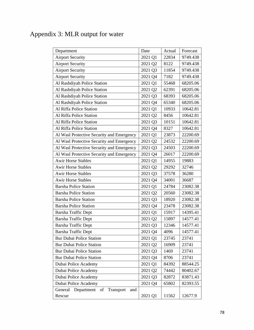
78
Appendix 3: MLR output for water
Department Date Actual Forecast
Airport Security 2021 Q1 22834 9749.438
Airport Security 2021 Q2 8122 9749.438
Airport Security 2021 Q3 11854 9749.438
Airport Security 2021 Q4 7182 9749.438
Al Rashdiyah Police Station 2021 Q1 55468 68205.06
Al Rashdiyah Police Station 2021 Q2 62391 68205.06
Al Rashdiyah Police Station 2021 Q3 68393 68205.06
Al Rashdiyah Police Station 2021 Q4 65340 68205.06
Al Riffa Police Station 2021 Q1 10933 10642.81
Al Riffa Police Station 2021 Q2 8456 10642.81
Al Riffa Police Station 2021 Q3 10151 10642.81
Al Riffa Police Station 2021 Q4 8327 10642.81
Al Wasl Protective Security and Emergency 2021 Q1 23873 22200.69
Al Wasl Protective Security and Emergency 2021 Q2 24532 22200.69
Al Wasl Protective Security and Emergency 2021 Q3 24503 22200.69
Al Wasl Protective Security and Emergency 2021 Q4 26017 22200.69
Awir Horse Stables 2021 Q1 14955 19883
Awir Horse Stables 2021 Q2 29292 32746
Awir Horse Stables 2021 Q3 37578 36280
Awir Horse Stables 2021 Q4 34001 36687
Barsha Police Station 2021 Q1 24784 23082.38
Barsha Police Station 2021 Q2 20560 23082.38
Barsha Police Station 2021 Q3 18920 23082.38
Barsha Police Station 2021 Q4 23478 23082.38
Barsha Traffic Dept 2021 Q1 15917 14395.41
Barsha Traffic Dept 2021 Q2 15897 14577.41
Barsha Traffic Dept 2021 Q3 12346 14577.41
Barsha Traffic Dept 2021 Q4 4096 14577.41
Bur Dubai Police Station 2021 Q1 23745 23741
Bur Dubai Police Station 2021 Q2 16909 23741
Bur Dubai Police Station 2021 Q3 1469 23741
Bur Dubai Police Station 2021 Q4 8706 23741
Dubai Police Academy 2021 Q1 84392 88544.25
Dubai Police Academy 2021 Q2 74442 80402.67
Dubai Police Academy 2021 Q3 82872 83871.43
Dubai Police Academy 2021 Q4 65802 82393.55
General Department of Transport and
Rescue 2021 Q1 11562 12677.9
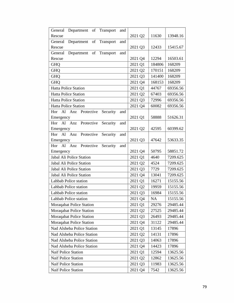
79
General Department of Transport and
Rescue 2021 Q2 11630 13948.16
General Department of Transport and
Rescue 2021 Q3 12433 15415.67
General Department of Transport and
Rescue 2021 Q4 12294 16503.61
GHQ 2021 Q1 184806 168209
GHQ 2021 Q2 170151 168209
GHQ 2021 Q3 141400 168209
GHQ 2021 Q4 168153 168209
Hatta Police Station 2021 Q1 44767 69356.56
Hatta Police Station 2021 Q2 67403 69356.56
Hatta Police Station 2021 Q3 72996 69356.56
Hatta Police Station 2021 Q4 60082 69356.56
Hor Al Anz Protective Security and
Emergency 2021 Q1 58888 51626.31
Hor Al Anz Protective Security and
Emergency 2021 Q2 42595 60399.62
Hor Al Anz Protective Security and
Emergency 2021 Q3 47642 53633.35
Hor Al Anz Protective Security and
Emergency 2021 Q4 50795 58851.72
Jabal Ali Police Station 2021 Q1 4640 7209.625
Jabal Ali Police Station 2021 Q2 4524 7209.625
Jabal Ali Police Station 2021 Q3 7729 7209.625
Jabal Ali Police Station 2021 Q4 13041 7209.625
Lahbab Police station 2021 Q1 16271 15155.56
Lahbab Police station 2021 Q2 19959 15155.56
Lahbab Police station 2021 Q3 16984 15155.56
Lahbab Police station 2021 Q4 NA 15155.56
Moraqabat Police Station 2021 Q1 29276 29485.44
Moraqabat Police Station 2021 Q2 27525 29485.44
Moraqabat Police Station 2021 Q3 26493 29485.44
Moraqabat Police Station 2021 Q4 31122 29485.44
Nad Alsheba Police Station 2021 Q1 13145 17896
Nad Alsheba Police Station 2021 Q2 14131 17896
Nad Alsheba Police Station 2021 Q3 14063 17896
Nad Alsheba Police Station 2021 Q4 14423 17896
Naif Police Station 2021 Q1 12594 13625.56
Naif Police Station 2021 Q2 12862 13625.56
Naif Police Station 2021 Q3 11983 13625.56
Naif Police Station 2021 Q4 7542 13625.56
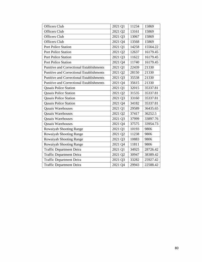
80
Officers Club 2021 Q1 11234 15869
Officers Club 2021 Q2 13161 15869
Officers Club 2021 Q3 13067 15869
Officers Club 2021 Q4 13568 15869
Port Police Station 2021 Q1 14258 15564.22
Port Police Station 2021 Q2 12637 16179.45
Port Police Station 2021 Q3 11622 16179.45
Port Police Station 2021 Q4 11740 16179.45
Punitive and Correctional Establishments 2021 Q1 22439 21330
Punitive and Correctional Establishments 2021 Q2 28150 21330
Punitive and Correctional Establishments 2021 Q3 35538 21330
Punitive and Correctional Establishments 2021 Q4 35615 21330
Qusais Police Station 2021 Q1 32015 35337.81
Qusais Police Station 2021 Q2 31535 35337.81
Qusais Police Station 2021 Q3 33160 35337.81
Qusais Police Station 2021 Q4 34182 35337.81
Qusais Warehouses 2021 Q1 29589 36435.65
Qusais Warehouses 2021 Q2 37417 36252.5
Qusais Warehouses 2021 Q3 37999 33897.76
Qusais Warehouses 2021 Q4 37575 33954.73
Rowaiyah Shooting Range 2021 Q1 10193 9806
Rowaiyah Shooting Range 2021 Q2 11238 9806
Rowaiyah Shooting Range 2021 Q3 10883 9806
Rowaiyah Shooting Range 2021 Q4 11811 9806
Traffic Department Deira 2021 Q1 34925 28726.42
Traffic Department Deira 2021 Q2 30947 38389.42
Traffic Department Deira 2021 Q3 33282 25927.42
Traffic Department Deira 2021 Q4 29943 22588.42