Ecological Modelling 165 (2003) 265–283

A growth model for gilthead seabream (Sparus aurata)

Juan M. Hernándeza,∗, Eucario Gasca-Leyvab, Carmelo J. Leónc, J.M. Vergarada Department of Quantitative Methods, University of Las Palmas de Gran, Canaria, c/Saulo Torón s/n, 35017 Las Palmas, Spain

b Centro de Investigación y de Estudios Avanzados del IPN (CINVESTAV), Unidad Mérida. Apdo. Postal 73-CORDEMEX,97310 Mérida, Yucatán, Mexico

c Department of Applied Economic Analysis, University of Las Palmas de Gran Canaria, c/Saulo Torón s/n, 35017 Las Palmas, Spaind Department of Biology, University of Las Palmas de Gran Canaria, c/Saulo Torón s/n, 35017 Las Palmas, Spain

Received 27 July 2001; received in revised form 7 August 2002; accepted 11 March 2003

Abstract

This paper presents a growth model for gilthead seabream (Sparus aurata), which is one of the most culture species in theMediterranean area. The model is designed by means of stochastic differential equations, and is based on previous researchfor other species [Modélisation de la Croissance des Poissons en Élevage, 1990]. Fish growth is assumed to be influencedby three fundamental factors: fish weight, water temperature, and ration size. The formulation incorporates fish physiologytheory, requiring fewer specific parameters than other bionenergetic models. Empirical data were obtained from culture in theCanary Islands waters for a 30-month period. Some simulations were run to validate the model. Although the influence ofwater temperature on fish growth might need to be refined, satisfactory results are obtained. Two environmental scenarios arealso examined, the “Atlantic” and “Mediterranean,” which vary in the annual cycles of water temperature. The results producesignificant differences in the growth patterns between both areas, suggesting potential economic implications for the cultivationof larger commercial sizes.© 2003 Elsevier Science B.V. All rights reserved.

Keywords:Gilthead seabream; Fish growth; Dynamical system; Validation; Simulation

1. Introduction

Controlling fish growth is one of the essential tasksin the aquaculture industry. Fish growth is influencedby a variety of factors, including fish weight, watertemperature, feeding rates, water quality, diet com-position, stocking densities, and environmental con-ditions (Brett, 1979). The interactions between thesefactors challenge the prediction of growth rates in afarm environment. This is generally approached by

∗ Corresponding author. Tel.:+34-928-458228;fax: +34-928-458225.

E-mail address:juanh@empresariales.ulpgc.es (J.M. Hernandez).

controlling some of the most important factors influ-encing growth.

Fish growth in aquaculture systems is usually an-alyzed by means of mathematical modeling. Modelsare constructed starting from the information accumu-lated through the long period of activity in fish farm-ing. Simulation has been the common tool to analyzedifferent aspects of fish growth in these models. Thus,due to their high commercial development, some spe-cific species has been extensively studied, such assalmonids (Corey et al., 1983; Bjorndal, 1990; Sylviaand Anderson, 1993), trout (McNown and Seireg,1983; Logan and Johnston, 1992), shrimp and prawn(Leung, 1986; Karp et al., 1986; Leung and Shang,1989), catfish (Hogendoorn, 1983; Cacho, 1990;

0304-3800/03/$ – see front matter © 2003 Elsevier Science B.V. All rights reserved.doi:10.1016/S0304-3800(03)00095-4

266 J.M. Hernandez et al. / Ecological Modelling 165 (2003) 265–283

Nomenclature

C log-linear regression parameterCR(w, θ, r) conversion ratedRM/dt rate of change of the maximum

growth rationdwM/dt maximum fish growthD temperature adjusting parameterf1(w) weight functionf2(θ) thermal functionf3(r) ration functionH conversion rate adjusting

parameterm fish size parameterr normalized ration sizerc normalized cultivation rationrm normalized maintenance rationrM normalized maximum growth

rationro normalized optimal rationR ration sizeRm maintenance rationRM maximum growth rationw fish weightY(r) normalized conversion rateZ(r) normalized growth rate

Greek symbolsα first temperature function

parameterβ second temperature function

parameterγ conversion rate parameterθ water temperatureθM maximum lethal temperatureai minimum temperature in monthibi maximum temperature in monthiΓ other influencing factors parameter

Masser et al., 1991; Cacho et al., 1991), and tilapia(Fischer and Grant, 1994; Yi, 1998; Bocci, 1999).

The gilthead seabream (Sparus aurata) is one ofthe most cultured species in the Mediterranean area(FAO, 1997). The commercial activity started inGreece and Turkey in the early 1980s. Productionareas have spread throughout other countries, and it

has become predominant over other finfish species,mainly because of its ease for acclimation to captiv-ity and its initially high market price. In 1996 about488 farms were operating in more than 10 differentMediterranean countries. Their market share out oftotal seafood production has increased from 14.4% in1989 to 23% in 1995.

Accordingly, multiple studies for larvae and juve-nile sizes of gilthead seabream can be found in theliterature (Yúfera et al., 1995; Rodrıguez et al., 1997;Paspatis et al., 2000). Some experiments and prelim-inary attempts have also been carried on for farmingsizes (Porter et al., 1986; Hidalgo and Sierra, 1993;Rosenlund et al., 1996; Ellner et al., 1996; Molinaet al., 1997; Gamito, 1998). However, a specificgrowth model for adult seabream sizes in culturefarms has not been developed yet.

The Canary Islands constitute an archipelago lo-cated in the bio-geographic region known as Mac-aronesia, sited about 2 km south the coast of Spain inthe Atlantic Ocean. Seabream was introduced for fishfarming there since last 1980s, although the culture inoffshore floating cages did not start until 1994. Therelatively constrained European market accessibilityis a handicap for culture development in the islands.However, there are advantages due to adequate envi-ronmental conditions involving water temperature orwater quality. In this context, a simulation model canbe useful to examine factors influencing competitivein Canary Islands with respect to other industries inthe Mediterranean areas.

Simulation models for other species are usuallybased on bioenergetics (Cacho, 1990; Santha et al.,1991; Masser et al., 1991; Xiao-Jun and Ruyung,1992; McDonald et al., 1996; Yi, 1998; Gorokhova,1998; Cho and Bureau, 1998; Bocci, 1999). Thesemodels require costly experimental information todetermine how the different nutrients and factorsinfluence growth, and results can be subject to inac-curacy. The use of some theoretical knowledge aboutfish metabolism can bypass the need of complex ex-periments to determine model equations. Fish physi-ology has already been extensively developed (Brettand Groves, 1979; Brett, 1979) and has been appliedto some studies, as inMuller-Feuga (1990)for thearc-en-ciel trout (Oncorhynchus mykiss). Physiologi-cal aspects has also been included in other integratedculture models (Troell and Norberg, 1998). This type

J.M. Hernandez et al. / Ecological Modelling 165 (2003) 265–283 267

of shortcut modeling incorporates the most represen-tative control variables generally used by farmers,such as ration size or water temperature, assum-ing constant diet composition. Thus, these modelsdo not aim at precisely establishing the effect ofdiet composition on growth, but rather at obtainingsome general results which might be useful for farmmanagement.

This paper presents a growth model for giltheadseabream in culture farms. The model incorporatessome elements from fish physiology theory. Parame-ters have been determined from commercial growthdata and literature. An extensive model validationis also included, obtaining satisfactory results. Asan illustration, two alternative scenarios are simu-lated: “Atlantic” and “Mediterranean.” This compar-

Fig. 1. Bioeconomic model for gilthead seabream.

ison shows the influence of location on industrialreturns.

2. Model description

The growth model we present in this paper is partof a more extensive bioeconomic model for giltheadseabream. In general, a bioeconomic model has to in-clude the interactions between management decisionand economic results obtained in fish farming.Fig. 1shows the most relevant variables in the seabreammodel and their inter-relations. Four submodels areincluded: biological, environmental, production man-agement, and economic. The bioeconomic model isused to obtain some economic indicators in a seabream

268 J.M. Hernandez et al. / Ecological Modelling 165 (2003) 265–283

production farm, as annual production, average costs,internal rates of return, etc. Moreover, simulation ofdifferent scenarios permits to find relevant informa-tion for the industry, as the optimum farm size, rela-tive competitiveness and cost minimization. We centeron the biological part of the model, that is, the growthmodel.

The growth model is formulated by means ofstochastic differential equations, and was imple-mented on a computer using a system dynamicsapproach (Forrester, 1961). This methodology hasbeen extensively used to build models that not onlyreferred to aquaculture system (Santha et al., 1991;Fischer and Grant, 1994; Montoya et al., 1999), butalso to describe other ecological models (Gorokhova,1998; Grasso, 1998). From a numerical point of view,an Euler integration method with a time step of 1day was adopted. A list of the variables and parame-ters in the model and their description is included inAppendix A.

Empirical growth data of gilthead seabream wereutilized for parameter estimation and validation pur-poses. They were collected at commercial farmssited in Melenara Bay, Canary Islands, between 1994and 1996. These data include monthly mean weightsampling for fishes in six offshore floating cages. Intotal, there are 10 different samples, since some ofthe cages included two samples of fish stocked atdifferent weight and time periods. The total numberof individuals analyzed was around 198,000.

2.1. Assumptions

The model includes three essential factors influ-encing fish growth in captivity. These are fish weight,water temperature, and ration size. In order to abstractfrom other possible factors, the following assumptionsare made:

(a) Water quality is optimal. Lack of water qualitycannot be considered a restriction for the con-ditions in the Canary Islands. Water circulationis guaranteed due to a Gulfstream branch go-ing through this world area. Therefore, dissolvedoxygen and nitrogen–ammonia can be easilymaintained around optimum values.

(b) Stocking density restrictions are not considered.Fingerlings are assumed to grow in low density

until they reach commercial size. That is, criticaldensity values were never obtained in commercialcage management.

(c) Diet composition is assumed to be fixed. This wasconstant over the field experiments, and based onthe same type of food already tested by feed pro-ducers. Thus, the question of feed quality is notconsidered as this is not really a control variablefor fish producers.

As it is shown inSection 3, these simplifications donot have significant influence in model validation.

2.2. Model description

Factors influencing fish growth are inter-related ina complex way, involving environmental aspects andthe genetic and fenotipic characters of the organism.We assume that the three essential factors mentionedabove are aggregated according to a multiplicativefunctional form, that is

dw

dt= Γf1(w)f2(θ)f1(r). (1)

Expression dw/dt is weight increase,f1(w) is theweight function, f2(θ) is the thermal function, andf3(r) is the ration function. ParameterΓ is exoge-nous and incorporates all other factors influencinggrowth. This general model closely reflects princi-ples of fish physiology (Brett, 1979; Ricker, 1979).The expression was first considered in growth mod-els for salmonids (Stauffer, 1973), and later appliedto other species (Corey et al., 1983; Muller-Feuga,1990). Next we describe each function separately. Thefunctional specifications and some of the parametersincluded are taken fromMuller-Feuga (1990).

2.2.1. The weight functionWeight function is assumed to be log-linear (Ricker,

1979). Thus, an increase in weight is positively relatedto fish weight, but with a smaller percentage as thesize rises. That is

f1(w) = Cwm. (2)

This expression has been more recommendable thanother growth functions for seabream in some empiricalstudies (Gamito, 1998). The parameterm must takevalues lower than one (m < 1). This parameter has

J.M. Hernandez et al. / Ecological Modelling 165 (2003) 265–283 269

been estimated for hot blood vertebrates, obtaining avalue of 0.7 (Brett and Groves, 1979).

2.2.2. The thermal functionFunctionf2(θ) is based on exponential forms. It in-

cludes maximum and minimum limits of water tem-perature beyond which growth is not possible. We haveadopted the following expression:

f2(θ) = D(eα(θM−θ) − eβ(θM−θ)). (3)

The variableθ = θ(t) represents water temperaturein time t. ParameterθM is the maximum temperaturefor which growth is possible under culture conditions.Expression (3) nulls forθ = θM. Values for the otherparameters determine the minimum temperature andvaries across species.

In order to include a cyclical variation of this vari-able over the seasonal year, a stepwise function ofmonthly uniform variables has been adopted forθ.Thus,

θ(t) ∼ Unif (ai, bi), t ∈ (ti, ti+1), i ∈ {1, 2, . . . },(4)

whereai andbi are the minimum and maximum tem-perature in monthi, respectively.

2.2.3. The ration functionWe define ration size (R = R(t)) as the total amount

of feed offered to fish from the stocking time to timet. Ration size is related to fish appetite, ranging fromstarvation (R = 0) to maximum ration size (R = RM).The ration function is defined in some bioenergeticsmodels using the daily ration size (dR/dt) (Stauffer,1973; Corey et al., 1983; Cacho, 1990). However,this approach requires the inclusion of complex ex-pressions related with temperature and fish weight.Moreover, new parameters needs to be introduced, sosubstantial amount of data are necessary to correctlyestimate the ration function. We can get around thisproblem by considering a normalized ration size (r).This variable is defined as the ratio between dailyration size over daily maximum growth ration, that is,

r = dR/dt

dRM/dt. (5)

This variable takes values between 0 and 1. We callrM = 1 the normalized maximum ration size.

Empirical observation of seabream ranching in-dicates that farmers tend to follow a constant ruleof thumb in feed management which is maintainedthrough the harvesting time according to recommen-dations from feed suppliers. Thus, farmers can beassumed to manage feeding rates according to a con-stant percentage of the normalized maximum rationsize (r). Since this percentage is independent of thefish weight and temperature, modelization is simpleand results easy to interpret.

The relationship between the normalized ration sizeand fish growth follows directly from fish physiology(Brett, 1979). Some singular levels of the normalizedration size can be found related to fish growth. Thereexists a normalized maintenance ration (rm), where thefish inputs and expenditures of energy are equilibratedand the growth is zero. We can find for higher per-centages the normalized optimal ration (ro), where aminimum food conversion rate (feed supplied/weightgain) is obtained.

In commercial culture, the ration size usuallyranges between the optimal and the maximum rations.Feeding tables supplied by feed providers tend to bewithin these values, where a maximum technical–economic benefit for fish farms is obtained. This ra-tion level is called the normalized cultivation ration(rc) (Muller-Feuga, 1990; Talbot and Hole, 1994).

In order to describe the ration function, we introducethe normalized growth rateZ(r). This variable repre-sents fish growth rate as a percentage of the maximumgrowth rate. Thus, the ration function is defined as

f3(r) = Z(r)

Z(rc). (6)

That is, the effect of the normalized ration size onfish growth is modeled by its deviation from thenormalized cultivation ration size.Z(r) is defined as

Z(r) = r

Y(r), (7)

whereY(r) is the normalized conversion rate and alsotakes values between 0 and 1. The functionY(r) mustinclude some characteristics related to the singularlevels. That is, it should decrease between starva-tion and the normalized optimal ration, with a singlepoint in the normalized maintenance ration size and aminimum in the normalized optimal ration.Fig. 2 il-lustrates this function and the normalized growth rate.

270 J.M. Hernandez et al. / Ecological Modelling 165 (2003) 265–283

Fig. 2. Graphic representations ofY(r) and Z(r).

The following expression satisfies these conditionsand is adopted for modeling purposes,

Y(r) = r

(1 + c(1 − r)2

rm(1 − rm)2(r − rm)

), (8)

where parameterc is determined by the value ofro.The growth model can be used to derive the amount

of feed consumed for a fish to reach a specific size.In order to do this, it is necessary to transform thenormalized conversion rateY(r) into a real conversionrate for different values ofw, θ, and r. We note thereal conversion rate as CR(w, θ, r). The amount offeed consumed is obtained by summing up the feedconsumed by a fish from the fry stage to the desiredsize. The relationship betweenY(r) and CR(w, θ, r) is

Table 1Model parameters, description, values, and sources

Parameter Description Value Source

m Fish size parameter 0.23 Statistical estimationθM Maximum lethal temperature 32.9◦C Ravagnan (1984)α Temperature function parameter −0.12 Muller-Feuga (1990)β Temperature function parameter −0.15 Muller-Feuga (1990)D Temperature adjusting parameter 4.93 Calibrationro Normalized optimal conversion rate 0.50 Brett (1979)rm Normalized maintenance ration 0.12 Brett et al. (1969), Muller-Feuga (1990)rc Normalized cultivation ration 0.80 Muller-Feuga (1990)r Normalized ration 1 CalibrationΓ Other influencing factors parameter 1 CalibrationH Conversion rate adjusting parameter D.O.T.a Statistical estimation and calibrationγ Conversion rate parameter D.O.T.a Statistical estimation and calibration

a D.O.T., depends on temperature.

shown in the following equation:

Y(r) = CR(w, θ, r)

[dwM/dt

dRM/dt

]w,θ

. (9)

Thus, the normalized conversion rate is equal to theproduct between the real conversion rate and the quo-tient between daily maximum fish growth (dwM/dt)and daily maximum growth ration (dRM/dt). It dependson weight and temperature. Estimates of this quotientand the rest of parameters are included in the follow-ing subsection.

2.3. Parameter estimation and calibration

The parameters included in the model are pre-sented inTable 1, with detailed description, values,

J.M. Hernandez et al. / Ecological Modelling 165 (2003) 265–283 271

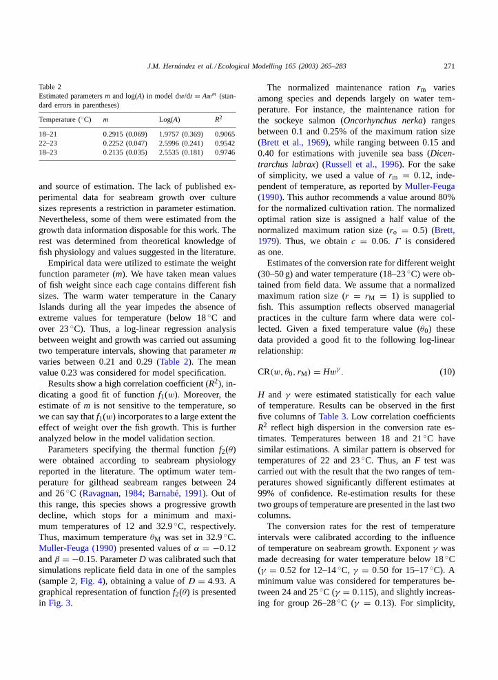
Table 2Estimated parametersm and log(A) in model dw/dt = Awm (stan-dard errors in parentheses)

Temperature (◦C) m Log(A) R2

18–21 0.2915 (0.069) 1.9757 (0.369) 0.906522–23 0.2252 (0.047) 2.5996 (0.241) 0.954218–23 0.2135 (0.035) 2.5535 (0.181) 0.9746

and source of estimation. The lack of published ex-perimental data for seabream growth over culturesizes represents a restriction in parameter estimation.Nevertheless, some of them were estimated from thegrowth data information disposable for this work. Therest was determined from theoretical knowledge offish physiology and values suggested in the literature.

Empirical data were utilized to estimate the weightfunction parameter (m). We have taken mean valuesof fish weight since each cage contains different fishsizes. The warm water temperature in the CanaryIslands during all the year impedes the absence ofextreme values for temperature (below 18◦C andover 23◦C). Thus, a log-linear regression analysisbetween weight and growth was carried out assumingtwo temperature intervals, showing that parametermvaries between 0.21 and 0.29 (Table 2). The meanvalue 0.23 was considered for model specification.

Results show a high correlation coefficient (R2), in-dicating a good fit of functionf1(w). Moreover, theestimate ofm is not sensitive to the temperature, sowe can say thatf1(w) incorporates to a large extent theeffect of weight over the fish growth. This is furtheranalyzed below in the model validation section.

Parameters specifying the thermal functionf2(θ)were obtained according to seabream physiologyreported in the literature. The optimum water tem-perature for gilthead seabream ranges between 24and 26◦C (Ravagnan, 1984; Barnabé, 1991). Out ofthis range, this species shows a progressive growthdecline, which stops for a minimum and maxi-mum temperatures of 12 and 32.9◦C, respectively.Thus, maximum temperatureθM was set in 32.9◦C.Muller-Feuga (1990)presented values ofα = −0.12andβ = −0.15. ParameterD was calibrated such thatsimulations replicate field data in one of the samples(sample 2,Fig. 4), obtaining a value ofD = 4.93. Agraphical representation of functionf2(θ) is presentedin Fig. 3.

The normalized maintenance rationrm variesamong species and depends largely on water tem-perature. For instance, the maintenance ration forthe sockeye salmon (Oncorhynchus nerka) rangesbetween 0.1 and 0.25% of the maximum ration size(Brett et al., 1969), while ranging between 0.15 and0.40 for estimations with juvenile sea bass (Dicen-trarchus labrax) (Russell et al., 1996). For the sakeof simplicity, we used a value ofrm = 0.12, inde-pendent of temperature, as reported byMuller-Feuga(1990). This author recommends a value around 80%for the normalized cultivation ration. The normalizedoptimal ration size is assigned a half value of thenormalized maximum ration size (ro = 0.5) (Brett,1979). Thus, we obtainc = 0.06. Γ is consideredas one.

Estimates of the conversion rate for different weight(30–50 g) and water temperature (18–23◦C) were ob-tained from field data. We assume that a normalizedmaximum ration size (r = rM = 1) is supplied tofish. This assumption reflects observed managerialpractices in the culture farm where data were col-lected. Given a fixed temperature value (θ0) thesedata provided a good fit to the following log-linearrelationship:

CR(w, θ0, rM) = Hwγ. (10)

H and γ were estimated statistically for each valueof temperature. Results can be observed in the firstfive columns ofTable 3. Low correlation coefficientsR2 reflect high dispersion in the conversion rate es-timates. Temperatures between 18 and 21◦C havesimilar estimations. A similar pattern is observed fortemperatures of 22 and 23◦C. Thus, anF test wascarried out with the result that the two ranges of tem-peratures showed significantly different estimates at99% of confidence. Re-estimation results for thesetwo groups of temperature are presented in the last twocolumns.

The conversion rates for the rest of temperatureintervals were calibrated according to the influenceof temperature on seabream growth. Exponentγ wasmade decreasing for water temperature below 18◦C(γ = 0.52 for 12–14◦C, γ = 0.50 for 15–17◦C). Aminimum value was considered for temperatures be-tween 24 and 25◦C (γ = 0.115), and slightly increas-ing for group 26–28◦C (γ = 0.13). For simplicity,

272 J.M. Hernandez et al. / Ecological Modelling 165 (2003) 265–283

Fig. 3. Graphic representation of the effect of temperature over fish growth (f2(θ)).

Table 3Estimated parametersγ and log(H) in model CR(w, θ0, rM) = Hwγ (standard errors in parentheses)

Parameters Water temperature,θ0 (◦C)

18 19 21 22 23 18–21a 22–23

Log(H) −0.703 (0.375) −0.783 (0.276) −0.764 (0.243) −0.069 (0.131) 0.065 (0.107) −0.736 (0.202) −0.102 (0.106)γ 0.422 (0.153) 0.434 (0.112) 0.454 (0.103) 0.121 (0.059) 0.080 (0.050) 0.435 (0.083) 0.116 (0.048)R2 0.386 0.518 0.796 0.322 0.207 0.565 0.217

a We have taken in this group values ofγ = 0.432 and log(H) = −0.743, inside the confidence intervals.

parameterH was maintained constant for all groupsabove 22 and below 21◦C, respectively.

Quotient [(dwM/dt)/(dRM/dt)]w,θ can be calcu-lated from estimated CR(w, θ, rM) andEq. (9). Thus,real conversion rate values can be obtained in themodel for any value of weight, temperature, and rationsize.

3. Model validation

Validation is a fundamental step in model build-ing. By means of validation the model becomes ac-ceptable for its intended use, guaranteeing a degree ofconfidence in simulation results. Data validation is notthe only standard to be applied. Other aspects to be

J.M. Hernandez et al. / Ecological Modelling 165 (2003) 265–283 273

dealt with are its agreement with previous theory andthe performance of the whole model (Rykiel, 1996;Klepper, 1997). The former has been previously con-sidered in the model construction (Brett, 1979). Here,three different analyses for validation are conducted:(a) fitness of the model; (b) sensitivity analysis; and(c) comparison of model predictions with field data.

3.1. Fitness of the model

The growthEq. (1) has been applied successfullyto other species (Stauffer, 1973; Corey et al., 1983;Muller-Feuga, 1990). Nevertheless, similarly to thelast author, an analysis of the specific growth for fielddata was conducted in order to test for the hypothe-sis of the multiplicative relationship among variables.This can be done because the specific growth is de-fined as the relative growth rate subtracting the effectof weight. Thus, the analysis of this variable for dif-ferent values of weight and temperature unveils thestructure of the remaining effects.

Table 4presents the specific growth for the field dataassuming that the effect of weight followsf1(w). Italso included the estimates of the variation coefficient,defined as the percentage of the standard deviationof data over their mean. This variable indicates thedifference among values in the same row or column.It is presented for a fixed temperature, VCw, and fora fixed weight, VCθ. It can be observed that VCwranges from 3.96 to 15.23%, while VCθ ranges from30.12 to 46.37%. Low values of VCw suggests that

Table 4Specific growth estimations for different temperatures and fish weights

Weight (g) Temperature

12 14 16 18 20 22 24 26 28 VCθ (%)

18 24.89 28.88 17.59 13.99 16.91 10.99 12.61 7.57 7.92 46.3727.5 25.34 36.03 19.25 15.10 17.37 9.89 12.61 12.38 12.38 46.4147.5 23.99 26.39 18.83 15.81 18.97 9.84 11.52 11.92 11.92 35.5070 22.24 25.02 17.43 16.46 19.99 10.00 12.56 12.99 12.99 30.12

115 23.50 26.86 17.93 14.12 19.26 10.57 11.81 11.53 11.53 36.06200 24.86 29.00 18.51 14.16 18.41 10.54 12.72 12.63 12.63 36.87375 26.31 31.57 19.19 14.25 19.00 11.19 13.01 13.21 13.21 38.88500 23.48 29.35 17.78 13.33 16.67 11.34 12.38 11.68 11.68 38.27

VCw (%) 5.24 11.82 3.96 7.13 6.59 5.64 3.98 15.23 14.18

It is also represented the variation coefficient, that is the percentage of the standard deviation of data over their mean for a fixed weight(VCθ) and for a fixed temperature (VCw).

f1(w) incorporates a high percentage of the effect ofweight on fish growth. Therefore, we can consider thatfunction f1(w) is fairly an acceptable way to modelizethe effect of weight on seabream growth. Alternatively,medium values of VCθ show that temperature is anessential growth component, as it is widely known andalso incorporated inEq. (1).

3.2. Sensitivity analysis

A sensitivity analysis provides the effect of changesin parameter specification on fish growth. This in-volves determining those parameters with a majorinfluence on disturbances of fish growth predictions.The analysis was conducted by means of successivesimulations, varying all parameters included in themodel 20% up or down of their initial baseline values.Table 5shows the ratio (% change in fish weight)/(%change in parameter value), calculated in mean val-ues, relative to each parameter after 2 years of cul-ture. Initial fish weight was 13 g. ParametersH andγ

were varied in every water temperature interval at thesame percentage. These parameters do not influencefish growth, so the respective sensitivity values arenot included.

First, we can observe inTable 5that the sensitivityof total feed consumption takes values higher thansensitivity of fish weight. This is because one of thecomponents in the model that describe the effect ofchanges in parameters over feed consumption is thevariation in fish weight gain.

274 J.M. Hernandez et al. / Ecological Modelling 165 (2003) 265–283

Table 5Sensitivity analysis of the model

Parameter Fish weight (%) Total feed consumption (%)

m 1.73 2.31α 6.13 7.60β 4.83 5.52D 1.25 1.70c 0.05 0.06rm 0.03 0.03rc 0.49 0.69r 0.18 1.00Γ 1.25 1.70H – 1.00γ – 2.23

The values represent the percentage of change in fish weight andtotal feed consumption due to an unitary percentage change inparameter.

In the validation of a model it is desired that pa-rameters with highest sensitivity are determined withhigh accuracy (Rykiel, 1996). In our case, the highestsensitivity parameters are those governing the effectof temperature (α, β, andD), followed by the weightfunction parameter (m). In fact, the most sensitivefactors in other fish growth models use to be thoserelated to temperature (Cacho, 1990) and weightfunction parameter (Bocci, 1999). The fish size pa-rameterm was statistically estimated from field dataandD was calibrated according to the best agreementbetween simulated and field data. However, asα andβ were taken from results for other species, somepredictive errors can be expected as water tempera-ture varies. More reliable values for these parameterscould be obtained from specific experiments withadult seabream, but they are not available in theliterature.

Ration function parameters (c, rm, rc, r) have rela-tively low influence on model variables. This indicatesthat little errors in the determination of the normalizedmaintenance, optimal or cultivation ration are not fun-damental in an adequate model predictability. Theseparameters were taken according to fish physiologyand literature results. The ration function formula wasalso obtained from fish physiology theory, so we canconsider it conceptually validated.

Finally, the sensitivity of the conversion rate param-eters (H andγ) is relatively high. However, as valuesof these parameters corresponding to temperatures ofthe Canary Islands waters (18–21◦C and 22–23◦C)

were statistically determined, results obtained can beaccepted. The rest was calibrated according to fishphysiology theory.

3.3. Comparison of model predictionswith field data

Essentially, the model was constructed to estimatethe seabream growth for different culture conditions.Thus, the replication of the field data is fundamentalto consider the model as satisfactory validated.

Since we have 10 samples of commercial fishgrowth for six different floating cages, we conducted10 model simulations to be compared with the realsamples. Simulations start at the same stocking timeand with the same initial weight as in each real sam-ple. Simulated and observed data are shown inFig. 4,covering a period from June 1994 (month 0) to De-cember 1996 (month 30).

Intuitively, predictions do closely reflect the fielddata for the most of the samples. However, somestationary perturbations can be observed. Field fishgrowth tends to be faster than predictions from Juneto September and slower from December to March.This reflects some kind of disagreement in the effectof water temperature on fish growth.

Intuitive observations can be tested using appro-priate statistical indicators. We have included someof them recommended by system dynamics modelers(Sterman, 1984; Barlas, 1989). They are the coeffi-cient of determination (R2), the root mean square error(RMSE) and the Theil’s inequality coefficient (U) fordata variations. The last one is a nonparametric statis-tics which measures the level of discrepancy betweenobserved and simulated data. It can be split in threepercentage components: bias, variation, and covaria-tion component, indicating where the major discrep-ancy takes place.

Table 6presents the above validation measures foreach sample. Sample 2 does not really represent modelvalidation because this sample was used to calibratethe thermal function. However, the rest of samplesuses to exhibit large values ofR2 combined with lowRMSE, except for those ones with little number ofobservations. Moreover, coefficientU shows satisfac-tory values (below 0.20), showing not high discrepan-cies between simulated and field data. The percentagecomponents of the Theil coefficient exhibit low bias

J.M. Hernandez et al. / Ecological Modelling 165 (2003) 265–283 275

Fig. 4. Observed (continuous line) and simulated (pointed line) data samples for fish growth in six different floating cages.

276 J.M. Hernandez et al. / Ecological Modelling 165 (2003) 265–283

Table 6Statistical results for each sample (S) of real and simulated data

S1 S2 S3 S4 S5 S6 S7 S8 S9 S10

Observations 11 23 10 7 10 5 17 10 12 10R2 0.93 0.77 0.89 0 0.94 0 0.88 0.05 0.85 0.45RMSEa 5.14 6.46 7.09 2.97 7.94 1.27 7.04 4.12 22.0 9.17Theil coefficient 0.09 0.16 0.11 0.25 0.11 0.10 0.19 0.29 0.16 0.18Bias (UM) 0.10 0 0.05 0.02 0.10 0.32 0.05 0 0 0.02Variance (US) 0.38 0.02 0.41 0.41 0.61 0.26 0.68 0.86 0.24 0.27Covariance (UC) 0.52 0.98 0.54 0.57 0.29 0.42 0.27 0.14 0.76 0.71

Sample 2 has been taken for model calibration.a Root mean square error.

components for the largest samples. However, exclud-ing sample 2, variation component uses to take rela-tively large values. These results show that the modelreproduces quite well the observed data in their meanvalue, although there are some discrepancies in thevariance.

The highly significant sensitivity of the thermal pa-rameters presented inSection 3.2can serve as an ex-planation of the observed errors between simulatedand field data. Thermal parameters have been takenfrom literature, so it is possible that the model doesnot reflect exactly the real influence of temperatureon fish growth. Thus, somewhat poorer predictions forfish growth and conversion rates could be expected forculture in more extreme water temperatures, such asin the Mediterranean area.

On the contrary, model results show relative coher-ence with evidence in the Mediterranean area.Table 7

Table 7Conversion rates generated by the model for different normalizedration sizes (r) and harvest weights

Weight (g) Ration size(Canary Islands)

Ration size(Mediterranean Sea)

0.6 0.8 1 0.6 0.8 1

200 0.85 0.96 1.15 0.92 0.97 1.16300 1.02 1.13 1.35 1.23 1.39 1.66400 1.09 1.26 1.51 1.22 1.51 1.85500 1.12 1.34 1.64 1.34 1.50 1.85600 1.17 1.36 1.67 1.64 1.64 1.94700 1.30 1.39 1.69 1.76 1.96 2.30

It is considered temperature from waters surrounding the Ca-nary Islands (16–25◦C) and the Mediterranean Sea (west coast,12–25◦C), respectively.

shows the conversion rates generated by the model forthree different rationing levels (60, 80, and 100%) andtwo different scenarios: “Mediterranean” (west coast,12–25◦C) and “Atlantic” (Canary Islands, 16–25◦C).Runs were beginning in May. We can compare the sim-ulation data for the “Atlantic” scenario with the his-torical conversion rates (Table 8). Using a parametrictest (Johnston, 1984), no significant differences wereshown between field and simulated data forr = 1 with99% confidence. This result validates the hypothesisof maximum ration size in feeding rates.

As expected, conversion rates inTable 7 aregreater for the “Mediterranean” scenario than for the“Atlantic,” due to the effect of water temperature onfeeding. Simulated conversion rates for ration sizesbetween 80 and 100% in the Mediterranean are verysimilar to those reported for reaching selected size(400 g), as shown inBendag (1995). These studieshave been conducted from culture in waters of Tunisia.

Moreover, other data generated for the “Mediter-ranean” scenario were compared to other results pre-sented in the literature. The approximate time (12

Table 8Observed conversion rate (CR) data for different fish weights (w)in four floating cages (L1, L2, L3, L4)

Weight (g) L1 L2 L3 L4

200–240 0.96 1.44 1.21 1.43240–280 1.15 1.47 1.41 1.58280–320 1.33 1.6 1.55 1.7320–360 1.4 1.56 1.62 –360–400 1.51 1.69 1.67 1.8400–450 1.57 – 2.47 1.9450–500 2.17 1.68 – –

J.M. Hernandez et al. / Ecological Modelling 165 (2003) 265–283 277

months) needed to reach selected size (400 g) wasfound to be similar to that published bySahin (1995),who uses water temperature intervals in the coasts ofTurkey (12–26◦C). In contrast, water along the Frenchcoast can dip below 12◦C, which cause a pause ingrowth, requiring between 18 and 23 months to reachthe same size (De La Pomelie, 1995).

In balance, although there would be need of somerefinement in modeling the effect of water temperatureon fish growth, the simulated results adjust quite fineto real evidences in the Canary Islands and in certainareas of the Mediterranean Sea.

4. Discussion

Gilthead seabream growth in captivity has not beenextensively studied by means of dynamic models yet.This growth model incorporates results around the fishphysiology theory in order to simplify the equationsand to obtain practical managerial recommendationsfor fish farmers.

In contrast, other growth models consider themetabolic characteristics of the fish, obtaining moreadjusted models while using a lot of experimentaldata (Cacho, 1990; Cho and Bureau, 1998). However,fish experiments are usually conducted for fingerlings(Bocci, 1999), so bioenergetic models can conveycertain uncertainty for culture sizes. These technicalproblems increase for more complex and integratedmodels (Van Winkle et al., 1998). The model pre-sented in this paper has been constructed using datacollected from commercial culture. The satisfactoryresults obtained in validation testing allows the modelto be used to analyze the characteristics of the pro-ductivity and economy of seabream culture.

In particular, harvest weight is one of the main con-trol factors to be considered in fish farming. Largersizes tend to be more valuable than small ones, show-ing higher prices in the market. However, costs ofproduction also increase with size. The problem hasbeen analyzed from an economic point of view inBjorndal (1988), Arnason (1992), Heaps (1993)andMistiaen and Strand (1999)among others. In thesepapers, the theoretical results obtained are appliedto some species, including seabream (Mistiaen andStrand, 1999). However, since the considered growthmodels do not include the specific metabolic and

fenotipic characteristics of the species, results can notbe extrapolated when external factors are changed.Biological conditions are essential restrictions forattaining some sizes with a commercial objective.In fact, evidence in commercial practice shows thatlarge sizes (around 700 g), are not cultivated in theMediterranean region, while it is actually viable inthe Atlantic. Our model, as validated for changingexternal factors, can be used to provide some in-sights about the harvest weight problem for these twodifferent environmental conditions.

We have conducted simulations of the model withthe aim of analyzing the characteristics of the produc-tion function in the two scenarios introduced above,i.e. the “Mediterranean” and the “Atlantic.”Fig. 5shows the simulated growth curves for the two sce-narios, with ration sizes of 60, 80, and 100%, respec-tively. The initial month for simulations was May.The model simulations show substantial differencesin fish growth between soft and extreme water tem-perature areas. Weight gain in the “Atlantic” is morecontinued than in the “Mediterranean” scenario. Thelatter presents higher variations of the growth rate,due to stationary changes in temperature. The lowestgrowth rate inFig. 5 (right) corresponds to wintertime, when temperatures reach values around 12◦C,while it becomes more accelerated in summer time.The total effect is that fish weight grows slower in theMediterranean area than in the specific Atlantic one.

Fig. 5 also shows a sample of the effect of rationsize on fish growth. The higher the ration size, thefaster the fish attains market sizes. Nevertheless, thiseffect is not linear. There are not relative high differ-ences in growth rate between 80 and 100% normal-ized ration size. However, the reduction to 60% has amore significant effect.

The specific substitution rate between harvestingtime and ration size is represented inFig. 6. The curvelines represent the combinations of normalized rationsize and harvesting time that are needed to obtaina given harvest weight (isoquants). Harvest weightsinclude values from 300 to 700 g, that are commonmarket sizes. The decreasing and strictly convex formof these curves shows a non-linear substitution rela-tionship between both factors. The curves describethe technology of the firm. The farmer can be seen asinvolved in a cost minimization problem with harvest-ing time, normalized ration size, and harvest weight

278J.M

.H

erna

nd

ez

et

al./E

colog

ical

Mo

de

lling

16

5(2

00

3)

26

5–

28

3Fig. 5. Simulated fish growth of seabream for different ration sizes in the Atlantic scenario (left) and the Mediterranean scenario (right). Initial fish weight is 13 g and thestocking time is May.

J.M.

He

rnan

de

ze

ta

l./Eco

logica

lM

od

ellin

g1

65

(20

03

)2

65

–2

83

279

Fig. 6. Combinations of normalized ration size and harvesting time to obtain a given harvest weight (isoquants) in the production of gilthead seabream. Left: Atlantic scenario;right: Mediterranean scenario. Harvest weights are considered since 300 g until 700 g.

280 J.M. Hernandez et al. / Ecological Modelling 165 (2003) 265–283

as the control variables. First results obtained with themodel show that optimal decision approach observedmanagerial recommendations, that is a normalized ra-tion size ofr = 80% (León et al., 2001).

The comparison of both maps inFig. 6 indicatessome of the differences in the production process be-

Fig. 7. Total feed supplied to an individual fish with respect to harvest weight in both scenarios. We consider three different normalizedration sizes: (a) 60%, (b) 80%, and (c) 100%.

tween both geographical areas. For instance, for agiven ration size it is observed that the time necessaryfor a fish to get any size is clearly shorter in the At-lantic than in the Mediterranean scenario. That is, fora normalized ration size ofr = 80%, the time spentfor a 400 g final size is 341 days in the former, while

J.M. Hernandez et al. / Ecological Modelling 165 (2003) 265–283 281

is 432 days in the latter. This difference increase withharvest weight. Longer periods of cultivation involvespecific costs of production, which could make the cul-ture of larger sizes unprofitable. As an example, it canbe observed that the minimum period for fish sizes of700 g in the Mediterranean scenario is around 2 years.However, these sizes can be obtained in the Atlanticscenario with 531 harvesting days.

The difference in the harvesting days between thescenarios is aggregated to the significant discrepan-cies in the conversion rates presented inTable 7.Fig. 7 shows this total feed supplied for the consid-ered commercial sizes in both areas, assuming a nor-malized ration size of 60, 80, and 100%, respectively.It can be observed that the gap of feed expenditurebetween the two scenarios is increased for big sizesin the three cases. The widest gap for sizes over700 g is obtained for the observed managerial practiceof 100%.

Therefore, farms located in the Mediterranean sce-nario must get around the two serious handicaps ofhigh feeding costs and high harvesting times in theproduction of large commercial sizes. These factorsimpinge subsequent increments in other costs, suchas labor. Thus, the economic results for farms locatedin the Atlantic scenario seem to be clearly advanta-geous. However, for the Atlantic scenario it would benecessary to take also into account the problem of dis-tance to demand located in center and south Europe,which leads to higher transport cost. The market ex-perience has evidenced a rather good profitability forculture activities at the Canary Islands (Gasca-Leyva,1999).

5. Conclusions

The present model represents gilthead seabreamgrowth in aquaculture farms from fry to commercialsizes. It is formulated by means of stochastic differen-tial equations and it is implemented into the computerusing a System Dynamics approach. It is based onother models built for other species (Muller-Feuga,1990). The model has been validated from differentaspects. Nevertheless, the influence of water temper-ature on fish growth might need to be revisited infuture research as long as specific experiments withadult seabream sizes become available.

Fish growth has been modelized using some resultsfrom fish physiology theory. This approach substan-tially reduces the number of specific parameters whichwere necessary for model building. Moreover, rationsize has been introduced in a normalized way, assum-ing farmers supply the same percentage of the maxi-mum ration size through all the harvesting time. Thispractical rule of thumb has been observed in producerspractice. The theoretically based structure can be alsoextrapolated more easily to build fish growth modelsfor other species.

Two different environmental scenarios have alsobeen examined in the model. They are the “Atlantic”scenario, with soft water temperatures, and the“Mediterranean” scenario, including more extremewater temperatures. The harvest weight problem wasanalyzed by means of simulations, obtaining divergentresults for both scenarios.

Acknowledgements

We thank Yolanda Santana Jiménez for assistancewith the statistical estimation of parameters.

Appendix A

Equationdescription

Expression

Fish growthdw

dt= Γf1(w)f2(θ)f3(r)

Weight function f1(w) = Cwm

Thermal function f2(θ) = D(eα(θM−θ) − eβ(θM−θ))

Ration function f3(r) = Z(r)

Z(rc)

Normalized rationsize

r = dR/dt

dRM/dt

Normalized growthrate

Z(r) = dw/dt

dwM/dt

Normalizedconversion rate

Y(r) = r

(1 + c(1 − r)2

rm(1 − rm)2(r − rm)

)

Real conversionrate

CR(w, θ0, rM) = Hwγ

Normalized-realconversion ratefunction

Y(r) = CR(w, θ, r)

[dwM/dt

dRM/dt

]w,θ

282 J.M. Hernandez et al. / Ecological Modelling 165 (2003) 265–283

References

Arnason, R., 1992. Optimal feeding schedules and harvesting timein aquaculture. Mar. Res. Econ. 7 (1), 15–35.

Barlas, Y., 1989. Multiple test for validation of system dynamicstype of simulation models. Eur. J. Oper. Res. 42, 59–87.

Barnabé, G., 1991. Acuicultura, vol. II. Omega, España.Bendag, M., 1995. Systémes de production du loup et de la

daurade. Elevage intensif en bassins en Tunisie. CIHEAMCahiers Options Méditerranéennes 14, 97–112.

Bjorndal, T., 1988. Optimal harvesting of farmed fish. Mar. Resour.Econ. 5, 139–159.

Bjorndal, T., 1990. The Economics of Salmon Aquaculture.Blackwell Scientific Publications, Oxford.

Bocci, M., 1999. Modelling the growth of Nile Tilapia(Oreochromis niloticus) feeding on natural resources enenclosures in Laguna de Bay (Philippines). Ecol. Model. 119,135–148.

Brett, J.R., 1979. Environmental factors and growth. In: Hoar,W.S., Randall, D.J., Brett, J.R. (Eds.), Fish Physiology, vol. 8.Academic Press, London, pp. 599–676.

Brett, J.R., Groves, R.D.D., 1979. Physiological energetics. In:Hoar, W.S., Randall, D.J., Brett, J.R. (Eds.), Fish Physiology,vol. 8. Academic Press, London, pp. 279–347.

Brett, J.R., Shelbourn, J.E., Shoop, C.T., 1969. Growth rate andbody composition of fingerling sockeye salmon,Oncorhynchusnerka, in relation to temperature and ration size. J. Fish. Res.Board Can. 26, 2363–2394.

Cacho, O.J., 1990. Protein and fat dynamics in fish. A bioenergeticmodel applied to aquaculture. Ecol. Model. 50, 33–56.

Cacho, O.J., Hatch, U., Kinnucan, H., 1991. Optimal control offish growth. Am. J. Agric. Econ. 73, 174–183.

Cho, C.Y., Bureau, D.P., 1998. Development of bioenergeticmodels and theFish-PrFEQ software to estimate production,feeding ration and waste output in aquaculture. Aquat. LivingResour. 11, 199–210.

Corey, P.D., Leith, D.A., English, M.J., 1983. A growth modelfor Coho Salmon including effects of varying ration allotmentsand temperature. Aquaculture 30, 125–143.

De La Pomelie, C., 1995. L’elevage du bar et de la dauradeen France: viabilité économique des systémes de production.CIHEAM Cahiers Options Méditerranéenne 14, 79–89.

Ellner, S., Neori, A., Krom, M.D., Tsai, D., Easterling, M.R., 1996.Simulation model of recirculating mariculture with seaweedbiofilter: development and experimental test of the model.Aquaculture 143, 167–184.

FAO, 1997. The World State of Fishery and Aquaculture. Roma,Italy.

Forrester, J.W., 1961. Industrial Dynamics. Productivity Press, 464pp.

Fischer, G.W., Grant, W.E., 1994. Use of native predator to controlovercrowding in warm-water polyculture ponds: simulation ofa tucunare (Cychla monoculus) tilapia (Oreochromis niloticus)system. Ecol. Model. 72 (3/4), 205–227.

Gamito, S., 1998. Growth models and their use in ecologicalmodelling: an application to a fish population. Ecol. Model.113, 83–94.

Gasca-Leyva, E., 1999. Bioeconomıa del cultivo de la dorada(Sparus aurata). Ph.D. thesis, Department of Biology,University of Las Palmas de Gran Canaria, 228 pp.

Gorokhova, E., 1998. Exploring and modeling the growth dynamicsof Mysis mixta. Ecol. Model. 110, 45–54.

Grasso, M., 1998. Ecological–economic model for optimalmangrove trade off between forestry and fishery production:comparing a dynamic optimization and a simulation model.Ecol. Model. 112, 131–150.

Heaps, T., 1993. The optimal feeding of a farmed fish. Mar. Resour.Econ. 8 (1), 89–99.

Hidalgo, F., Sierra, M.A., 1993. Modelización del crecimiento dedorada (Sparus aurata) en condiciones de crıa intensiva. ActasIV Congreso Nacional Acuicultura, España, pp. 115–119.

Hogendoorn, H., 1983. Growth and production of the Africancatfish, Clarias lazera (C&V). III. Bioenergetic relations ofbody weight and feeding level. Aquaculture 35, 1–17.

Johnston, W.E., 1984. Econometric Models. McGraw-Hill, NewYork.

Karp, L., Sadeh, A., Griffin, W.L., 1986. Cycles in agriculturalproduction: the case of aquaculture. Am. J. Agric. Econ. 68,553–561.

Klepper, O., 1997. Multivariate aspects of model uncertaintyanalysis: tools for sensitivity analysis and calibration. Ecol.Model. 101, 1–13.

León, C.J., Hernández, J.M., Gasca-Leyva, E., 2001. Costoptimization and input substitution in the production of giltheadseabream. Aquacult. Econ. Manage. 5 (3/4), 147–170.

Leung, P., 1986. Applications of system modeling to aquaculture.Agric. Eng. 5, 171–182.

Leung, P., Shang, Y., 1989. Modeling prawn productionmanagement systems: a dynamic Markov decision approach.Agric. Eng. 29, 5–20.

Logan, S.H., Johnston, W.E., 1992. Economics of commercial troutproduction. Aquaculture 100, 25–46.

Masser, M.P., Grant, W.E., Neill, W.H., Robinson, E.H., 1991. Asimulation model representing effects on dietary/protein ratioand water temperature on growth of channel catfish (Ictaluruspunctatus). Ecol. Model. 53, 17–35.

Molina, D.L., López, C.G., Vergara, J.M., Robaina, R.L., 1997. Acomparative study of sediments under a marine cage farm atGran Canaria Island (Spain). Martinique 97-Island Aquacultureand Tropical Aquaculture.

McDonald, M.E., Tikkanen, C.A., Axler, R.P., Larsen, C.P.,Host, G., 1996. Fish simulation culture model (FISH-C):a bioenergetics based model for aquacultural wasteloadapplication. Aquacult. Eng. 15 (4), 243–259.

McNown, W., Seireg, A., 1983. Computer aided optimum designand control of staged aquaculture systems. J. World Maricult.Soc. 14, 417–433.

Mistiaen, J.A., Strand, I., 1999. Optimal feeding and harvest timefor fish weight-dependent prices. Mar. Resour. Econ. 13, 231–246.

Montoya, R.A., Lawrence, A.L., Grant, W.E., Velaso, M., 1999.Simulation of nitrogen dynamics and shrimp growth in anintensive shrimp culture system: effects of feed and feedingparameters. Ecol. Model. 122, 81–95.

J.M. Hernandez et al. / Ecological Modelling 165 (2003) 265–283 283

Muller-Feuga, A., 1990. Modélisation de la croissance des poissonsen élevage. Rapports scientifiques et techniques de l’IFREMER.Institut Français de Recherche pour l’Exploitation de la Mer.

Paspatis, M., Maragoudaki, D., Kentouri, M., 2000. Self-feedingactivity patterns in gilthead sea bream (Sparus aurata), redporgy (Pagrus pagrus) and their reciprocal hybrids. Aquaculture190, 389–401.

Porter, C.B., Krom, M.D., Gordin, H., 1986. The effect of waterquality on the growth ofSparus auratain Marine Fish Ponds.Aquaculture 59, 299–315.

Ravagnan, G., 1984. L’élevage du loup et de la daurade envalliculture. In: Barnab, G., Billard, R. (Eds.), L’AquacultureDu Bar Et Des Sparidés. INRA Publications, Paris, pp. 435–446.

Ricker, W.E., 1979. Growth rates and models. In: Hoar, W.S.,Randall, D.J., Brett, J.R. (Eds.), Fish Physiology, vol. 8.Academic Press, London, pp. 677–749.

Rodrıguez, C., Pérez, J.A., Dıaz, M., Izquierdo, M.S.,Hernández-Palacios, H., Lorenzo, A., 1997. Influence of theEPA/DHA ratio in rotifers on gilthead seabream (Sparus aurata)larval development. Aquaculture 150, 77–89.

Rosenlund, G., Talbot, E., Hole, R., 1996. Potential gainsthrough alimentation/nutrition. Improvements in the grow-out.In: Seabass and Seabream Culture: Problems and Prospects.pp. 160–174.

Russell, N.R., Fish, J.D., Wootton, R.J., 1996. Feeding and growthof juvenile sea bass: the effect of ration and temperature ongrowth rate and efficiency. J. Fish Biol. 49, 160–174.

Rykiel, E.J., 1996. Testing ecological models: the meaning ofvalidation. Ecol. Model. 90, 229–244.

Sahin, M., 1995. Sea bass and bream in floating cages in Turkey.CIHEAM Cahiers Options Méditerranéennes 14, 57–63.

Santha, C.R., Grant, W.E., Neill, W.H., Strawn, R.K., 1991.Biological control of aquatic vegetation using grass carp:

simulation of alternative strategies. Ecol. Model. 59 (3/4), 229–245.

Sterman, J.D., 1984. Appropiate summary statistics for evaluatingthe historic fit for the system dynamic models. Dynamica 10 (2),51–66.

Stauffer, G.D., 1973. A growth model for salmonids reared inhatchery environments. Ph.D. thesis, Department of Zoology,University Washington, Seattle, WA.

Sylvia, G., Anderson, J.L., 1993. An economic policy model fornet-pen salmon farming. In: Hatch, U., Kinnucan, H. (Eds.),Aquaculture Models and Economics. Westview Press, Boulder,pp. 17–38.

Talbot, C., Hole, R., 1994. Fish diets and the control ofeutrophication resulting from aquaculture. J. Appl. Ichthyol. 10,258–270.

Troell, M., Norberg, J., 1998. Modelling output and retention ofsuspended solids in an integrated salmon-mussel culture. Ecol.Model. 110, 65–77.

Van Winkle, W., Jager, H.I., Railsback, S.F., Holcomb, B.D.,Studley, T.K., Baldrige, J.E., 1998. Individual-based modelof sympatric populations of brown and rainbow trout forinstream flow assessment: model description and calibration.Ecol. Model. 110, 175–207.

Xiao-Jun, X., Ruyung, S., 1992. The bioenergetics of the southerncatfish (Silurus meridionalis Chen): growth rate as a functionof ration level, body weight, and temperature. J. Fish Biol. 40,719–730.

Yi, Y., 1998. A bioenergetics growth model for Nile tilapia(Oreochromis niloticus) based on limiting nutrients and fishstanding ponds. Aquacult. Eng. 18, 157–173.

Yúfera, M., Fernández-Dıaz, C., Pascual, E., 1995. Feeding ratesof gilthead seabream (Sparus aurata), larvae on microcapsules.Aquaculture 134, 257–268.