Journal of Great Lakes Research xxx (2012) xxx–xxx

JGLR-00427; No. of pages: 9; 4C:

Contents lists available at SciVerse ScienceDirect

Journal of Great Lakes Research

j ourna l homepage: www.e lsev ie r .com/ locate / jg l r

A geostatistical approach to optimize water quality monitoring networks in largelakes: Application to Lake Winnipeg

Dan Beveridge a,c,⁎, André St-Hilaire a,c, Taha B.M.J. Ouarda a, Bahaa Khalil a, F. Malcolm Conly b,Leonard I. Wassenaar b, Emily Ritson-Bennett b

a Statistical Hydrology Research Group, INRS-ETE, University of Québec, 490 de la Couronne St. Québec City, QC, Canada G1K 9A9b National Water Research Institute, Environment Canada, 11 Innovation Blvd., Saskatoon, SK, Canada S7N 3H5c Canadian Rivers Institute, University of New Brunswick, Fredericton, NB., Bailey Hall, 10 Bailey Drive, P.O. Box 4400, Fredericton, NB, Canada E3B 5A3

⁎ Corresponding author at: Statistical Hydrology Reseaof Québec, 490 de la Couronne St. Québec City, QC, Canad

E-mail address: dan.beveridge@gmail.com (D. Bever

0380-1330/$ – see front matter © 2012 International Adoi:10.1016/j.jglr.2012.01.004

Please cite this article as: Beveridge, D., et acation to Lake Winnipeg, J Great Lakes Res

a b s t r a c t

a r t i c l e i n f o

Article history:Received 16 August 2011Accepted 21 November 2011Available online xxxx

Communicated by Ram Yerubandi

Keywords:Lake WinnipegWater qualityMonitoring network optimizationGeostatistics

Water quality monitoring in lakes is often done by regularly sampling water quality variables of interest atfixed stations. Station location is a critical component of monitoring network design. Geostatistical methodswere used to quantify redundancy in an intentionally dense network of lake stations on Lake Winnipeg, Can-ada. Water isotope samples (δ2H, δ18O) were collected approximately every 1–2 km during research cruisesin September–October 2009, for a total of 240 lakewide stations. Two statistical approaches were used to as-sess redundancy: 1) kriging, a spatial interpolation technique, was performed in a reduced multivariate spaceand kriging variance was used to assess the suitability of the sampled network configuration; and 2) LocalMoran's I values were calculated. Moran's I identified clusters of stations that were similar or different.Good kriging models were developed for both δ2H and δ18O. When assessed individually, a large number ofstations were identified as redundant but redundancy was based on the premise that all other stationsremained in the network. When the analysis was performed on clusters of stations, within each cluster, upto four stations could be removed without significant loss of information. Relationships of redundancywere confirmed by Local Moran's I values. In combination, these techniques identified stations that were sta-tistically important or redundant. This study emphasizes the importance of completing the evaluation of in-formation provided by an individual station with information from clusters of stations within a network.

© 2012 International Association for Great Lakes Research. Published by Elsevier B.V. All rights reserved.

Introduction

The large numbers of potential anthropogenic stressors thatthreaten lakes and rivers have led to the development of exten-sive water quality monitoring networks in many countries aroundthe globe. The primary objectives of water quality monitoring net-works vary for different countries and different jurisdictions butoften include some or all of the following: compliance of waterquality metrics with regulatory standards, comparison of parame-ter results to national guidelines (e.g. CCME, 2006), identificationof spatial or temporal trends in water quality (e.g. Blind et al.,1994), and the assessment of natural ranges of variability. Waterquality monitoring is critical to appropriately evaluate past andcurrent watershed practices and to inform future decision-making, as in adaptive management frameworks (CMP, 2007).From a broader statistical perspective, most water quality networkdesigns aim to reduce the uncertainty in estimating a variable orits associated descriptive statistics for a given region (Alfonso et

rchGroup, INRS-ETE, Universitya G1K 9A9.idge).

ssociation for Great Lakes Research.

l., A geostatistical approach t(2012), doi:10.1016/j.jglr.20

al., 2010). For instance, station locations may be selected to re-duce the error in the estimation of average nutrient (e.g. nitrate)concentrations for a given period in a lake.

Monitoring networks must have clearly defined objectives,both about what they are measuring, required levels of accuracy,spatial and temporal grain and extent, with an implementationpathway to meet those objectives. The design of a water qualitymonitoring network typically involves three steps: 1) identifica-tion of the water quality variables to be observed, 2) definitionof the frequency at which they should be measured and 3) iden-tification of station locations. Khalil and Ouarda (2009) providedan overview of the most commonly used methods for each ofthese three steps.

For the selection of spatial monitoring network locations, initialdesigns are often based on a theme of systematic sampling and by lo-gistic considerations, such as routine and reliable access, which isoften a challenge in remote regions. More sophisticated approachesincluding those based on entropy of information theory have alsobeen used (Alfonso et al., 2010; Krstanovic and Singh, 1992).

Approaches based on inter-site covariance have also been used todetermine where monitoring should occur or be maintained. Some ofthe simpler variance-based methods include the use of multiple

Published by Elsevier B.V. All rights reserved.

o optimize water quality monitoring networks in large lakes: Appli-12.01.004

Fig. 1. Map showing location of Lake Winnipeg with 240 sampling stations.

2 D. Beveridge et al. / Journal of Great Lakes Research xxx (2012) xxx–xxx

linear regression (Tirsch and Male, 1984) in which stations are suc-cessively treated as the dependant variable and the water quality pa-rameter is estimated using the other stations as independentvariables. The partial correlation coefficient can be calculated foreach configuration and subsequently compared.

The estimation of spatial covariance has also been used for net-work rationalization and extension (Sampson and Guttorp, 1992).Kriging has been used to rationalize and to assess the possibility ofenhancing water quality and meteorological station networks(Huang and Yang, 1998; Pardo-Iguzquiza, 1998). St-Hilaire et al.(2003) used kriging to assess a network of meteorological monitoringstations in Québec, Canada. In this study, kriging variance was one ofthe criteria used to compare networks with high and low samplingstation density.

Unlike monitoring of water quality in rivers and small lakes, waterquality sampling in large (e.g. area>10,000 km2) lakes offers the sta-tistical advantage of a continuous sampling space. Identification ofstation location is a trade-off between the desire to capture all ofthe variability of the targeted variable within the lake and the needto avoid redundancy in sampling.

The objective of this study was to adapt and implement a geosta-tistical approach to in-lake site selection for an intentionally densenetwork of monitoring stations located in Lake Winnipeg. The pro-posed methodology is presented first, followed by the isotopic dataused to test the feasibility of the approach. We believe this geostatis-tical approach will be broadly applicable to the assessment and objec-tive validation of lake water quality monitoring networks fornumerous water quality parameters of interest, e.g. nutrients andcontaminants.

Study site

Lake Winnipeg is the 11th largest lake in the world (23,750 km2),with a drainage area of approximately 1 million km2 (Fig. 1). In re-cent years, Lake Winnipeg has shown symptoms of eutrophicationfrom a number of important anthropogenic stresses, primarily fromhigh and increasing riverine phosphorus and nitrogen nutrient load-ings. This increase in nutrient loading is believed to be the leadingcause of massive blue-green algal blooms in the past decade(Environment Canada and Manitoba Water Stewardship, 2011).

These concerns have prompted new research on Lake Winnipegby federal and provincial departments. In 2003, the Province ofManitoba introduced an action plan to protect Lake Winnipeg. Aspart of this action plan they introduced an interim goal to decrease ni-trogen and phosphorous loadings to pre-1970 levels (http://www.gov.mb.ca/waterstewardship/water_quality/lake_winnipeg/, accessed 25January 2011). The Action Plan also recognized that research on waterquality was lacking and that new scientific information was requiredto better inform management practices affecting Lake Winnipeg.

Historically, diverse water quality parameters have been collectedat various times as part of scientific cruises on Lake Winnipeg. Fisher-ies and Oceans Canada began the most spatially intensive monitoringin Lake Winnipeg in 1969. It continued for only a few years but pro-vided a foundation for future monitoring (e.g., Brunskill, 1973;Brunskill et al., 1979). Subsequent water quality monitoring in LakeWinnipeg was more intermittent and opportunistic but intensifiedagain in 1999 when the Province of Manitoba initiated a long-termmonitoring program in the lake that included up to 14 stations. Theformation of the Lake Winnipeg Research Consortium (LWRC) in1998 and the provision of a research platform, the MV Namao, hasallowed greater access to Lake Winnipeg for both monitoring and re-search activities. As a result, regular water quality monitoring occursat up to 65 stationary lake stations, and supports research activitiesthat can improve the understanding of the water quality of Lake Win-nipeg and better inform monitoring programs (Environment Canadaand Manitoba Water Stewardship, 2011).

Please cite this article as: Beveridge, D., et al., A geostatistical approach tcation to Lake Winnipeg, J Great Lakes Res (2012), doi:10.1016/j.jglr.20

During the 2009 research cruise season between 14/09/2009 and04/10/2009, Environment Canada collected high spatial frequencywater isotope (δ18O and δ2H) data at intervals of approximately1–2 km. Although intended for other hydrological modeling pur-poses, these samples fortuitously represented a dense, oversamplednetwork of 240 locations throughout the lake that were used as atest case for the optimal geostatistical design and rationalization ofa monitoring network, presented here.

Materials and methods

This research effort focuses on the monitoring of lake water qual-ity. Various federal and provincial agencies have conducted limnolog-ical surveys on Lake Winnipeg, each associated with differentconfigurations of monitoring networks and sampling efforts. Someof the networks have as few as eight stations, while some federalagencies sample as many as 65 sites in Lake Winnipeg during theirsurveys.

This analysis uses water isotope samples collected from the lakesurface at approximately every 1–2 km linear distances as the re-search vessel traversed LakeWinnipeg during its visits to the ~65 reg-ularly sampled stations. The water isotope samples were collected forother hydrodynamic monitoring purposes (Zhao et al., this issue),since each of the three major riverine inputs (the Red, Winnipegand Saskatchewan Rivers) have unique water isotopic compositions.The result was a dense sampling effort of 240 locations throughoutLake Winnipeg (Fig. 1). We used this oversampled dataset as a testcase for optimizing our geostatistical approaches. It should be notedthat water isotopes are not a water quality parameter that is routinely

o optimize water quality monitoring networks in large lakes: Appli-12.01.004

3D. Beveridge et al. / Journal of Great Lakes Research xxx (2012) xxx–xxx

monitored. However, water isotopes are conservative tracers of thewater molecule (unlike nutrients that can be consumed and recycled)and represent a foundational tracer for lake circulation modeling andnutrient sampling scenario comparisons. All water samples collectedfor isotopic measurement were analyzed as fully described in Zhaoet al. (this issue), with a measurement error of +/−1 and 0.2‰ forδ2H and δ18O, respectively.

Comparing individual station locations using kriging

We used kriging (Krige, 1951; Matheron, 1963) to identify waterquality stations that contributed the most and least information toprediction maps. Kriging is a geospatial interpolation method thatpredicts the value of a single variable at an unmeasured location asa function of observed data from nearby locations. The spatial depen-dence (or relatedness) between sampling points is expressed usingsemivariograms. The semivariogram captures how the differences invalues of points change as a function of inter-station distance.

Experimental semivariograms quantify this spatial dependencyand are calculated as follows:

γ hð Þ ¼ 12N hð Þ

XN hð Þ

i¼1

zxiþh−zxi Þ

2�

ð1Þ

where N(h) is the number of observation pairs separated by dis-tance h with values zxi . A theoretical model is then fitted to the semi-variogram. The kriging estimator z x0ð Þ at a given point xo is the bestlinear unbiased estimator of mean parameters (Cressie, 1990):

z x0ð Þ ¼XN hð Þ

i¼1

λiz xið Þ ð2Þ

where z(xi) is the weighted observed value at the ith location, andλi is the unknown weight for the measured value at the ith location.There is an additional constraint in ordinary kriging in order tosolve the linear system of equations:

XN hð Þ

i¼1

λi ¼ 1: ð3Þ

Kriging produces an optimalmodel prediction, in the sense that botherror and bias are minimized (Journel and Huijbregts, 1978). The valueof a water quality variable at an unmeasured location is thus estimatedusing the spatial dependency determined between known points. Ordi-nary kriging assumes local stationarity of the mean (Armstrong, 1998)and an unknown constant trend component.

In addition to providing an unbiased estimate of the variable of in-terest, kriging provides an estimation of variance. Unlike variance inlinear regression models, kriging variance at an unsampled point(σ2(x0)) is not a measure of local estimation accuracy of the variablebut is a useful statistic that allows for comparison of network config-uration, as it is solely dependent on the overall covariance structure(which is a function of inter-station distance) and kriging weights(Deutsch and Journel, 1998):

σ2 x0ð Þ ¼ C 0ð Þ−XN hð Þ

i¼1

λi xið ÞC x0−xið Þ ð4Þ

where C(0) is the stationary variance, and C(x0−xi)is the covariancebetween the ith monitored point and the unsampled point of interest,as estimated by the semivariogram.

By definition, kriging variance is minimized in the kriging model.Hence, if when removing a sampling station a kriging map withhigher variance is produced, then that station is likely important to

Please cite this article as: Beveridge, D., et al., A geostatistical approach tcation to Lake Winnipeg, J Great Lakes Res (2012), doi:10.1016/j.jglr.20

retain in the monitoring network. Conversely, if after removing a sta-tion and no change in the variance map is observed, then that stationis likely redundant with its neighbors.

Prior to kriging, data were analyzed using techniques such as nor-mal QQ plots, trend analysis, and semivariogram clouds to determinewhether the water quality data require transformation or trendremoval.

Once the data were prepared for kriging, a semivariogram modelwas fit. Model fitting determines the optimum values of a few param-eters such as the sill, range, andminor range and anisotropy ratio. Therange is the distance at which the semivariogram model reaches thesill; beyond this distance, observations appear independent. Anisot-ropy is the presence of directional dependence, i.e. there is a differ-ence in the spatial covariance structure for different directions. Ifthe data are anisotropic, the direction of strongest correlation definesthe direction of the major range. The minor range is perpendicular tothe major range and its length relative to the major range isexpressed as the anisotropy ratio. Different mathematical functionswere used to model the semivariance, e.g. linear, spherical, Gaussianor exponential. The variogram functions were iteratively selected,based on the model that yielded the smallest nugget effect and RootMean Square Error (RMSE). The nugget effect represents measure-ment error or variation at a spatial scale finer than the data.

Improving model prediction with additional knowledge

The kriging method presented above used the geographical coordi-nates of in-lake water quality stations to interpolate the values ofwater quality parameters. However, other factors that influence waterquality must be taken into consideration, such as other measured dataand/or expert opinion. Such additional factors include bathymetry(lake bed elevation), the proximity of a water quality station to themouth of a contributing river, and known or assumedwater circulationpatterns. There are cases where two lake monitoring stations may be atextreme ends of the lake (different geographic coordinates) but shareequivalent distances to a major outlet. If one river is driving or affectingprocesses that are measured by δ18O and δ2H, then distance to a riveroutlet will be a more direct measure of the gradient. Although geo-graphic location and distance to major river outlets constitute a highlyredundant set of variables, our intent was to select the most predictivesubset from among this redundant set of variables.

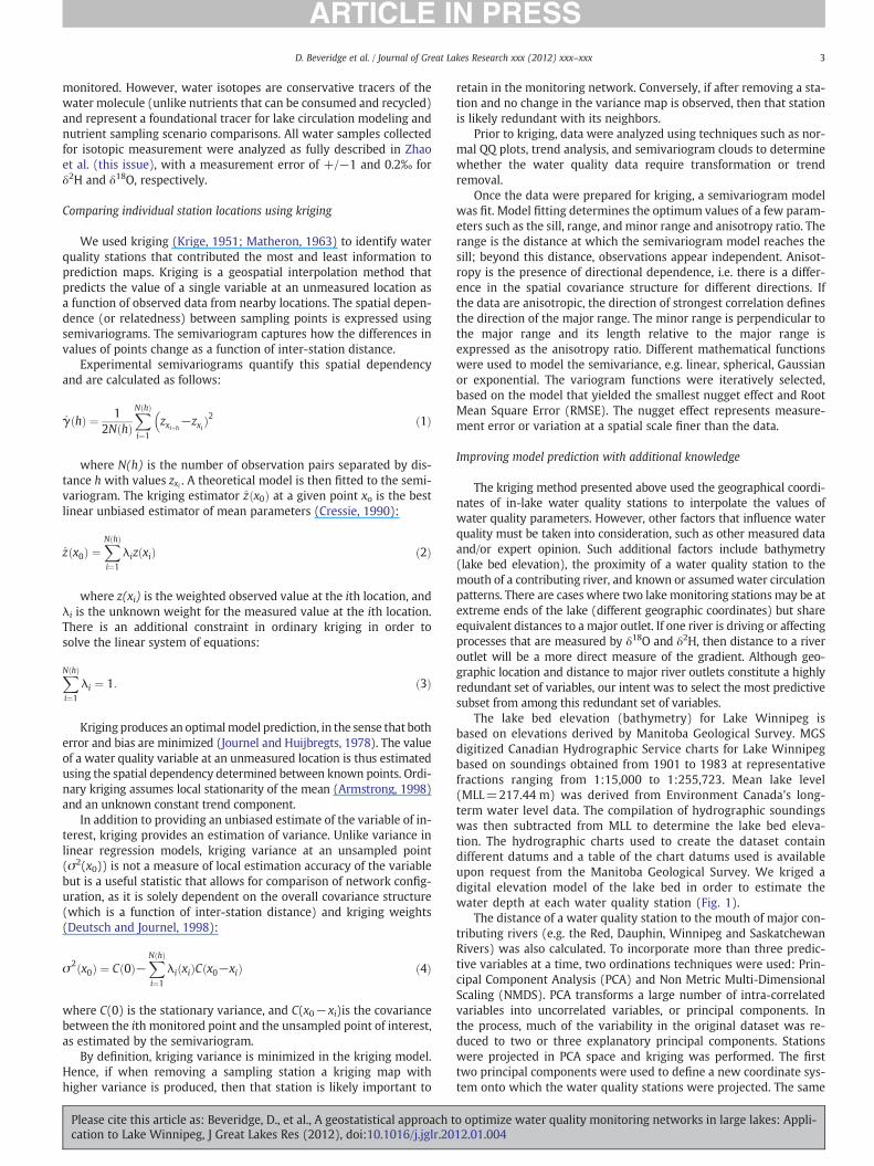
The lake bed elevation (bathymetry) for Lake Winnipeg isbased on elevations derived by Manitoba Geological Survey. MGSdigitized Canadian Hydrographic Service charts for Lake Winnipegbased on soundings obtained from 1901 to 1983 at representativefractions ranging from 1:15,000 to 1:255,723. Mean lake level(MLL=217.44 m) was derived from Environment Canada's long-term water level data. The compilation of hydrographic soundingswas then subtracted from MLL to determine the lake bed eleva-tion. The hydrographic charts used to create the dataset containdifferent datums and a table of the chart datums used is availableupon request from the Manitoba Geological Survey. We kriged adigital elevation model of the lake bed in order to estimate thewater depth at each water quality station (Fig. 1).

The distance of a water quality station to the mouth of major con-tributing rivers (e.g. the Red, Dauphin, Winnipeg and SaskatchewanRivers) was also calculated. To incorporate more than three predic-tive variables at a time, two ordinations techniques were used: Prin-cipal Component Analysis (PCA) and Non Metric Multi-DimensionalScaling (NMDS). PCA transforms a large number of intra-correlatedvariables into uncorrelated variables, or principal components. Inthe process, much of the variability in the original dataset was re-duced to two or three explanatory principal components. Stationswere projected in PCA space and kriging was performed. The firsttwo principal components were used to define a new coordinate sys-tem onto which the water quality stations were projected. The same

o optimize water quality monitoring networks in large lakes: Appli-12.01.004

Fig. 2. PCA scores of isotope stations plotted along the first two principal componentsof a PCA on the predictor variables.

Fig. 3. All 240 water isotope stations plotted in two-dimensional NMDS space.

4 D. Beveridge et al. / Journal of Great Lakes Research xxx (2012) xxx–xxx

approach is used to estimate flood quantiles (Chokmani and Ouarda,2004) and maximum water temperature (Guillemette et al., 2010).

Non Metric Multi-Dimensional Scaling (NMDS) is a non-parametric data reduction technique. While PCA attempts to build or-thogonal linear combinations or variables that maximize explainedvariance, NMDS aims at preserving the rank order of dissimilaritiesamong stations (Anderson et al., 2008). The input to NMDS is a matrixthat ranks dissimilarity between stations.

The primary assumption of NMDS is that the data are independentand identically distributed (Legendre and Legendre, 1998). The de-gree of correspondence between the distances among points inNMDS space and the matrix input by the user is (inversely) measuredby a stress function. Stress is the measure of how well sample rela-tions in the original dissimilarity matrix are preserved in the low-dimensional configuration. The configuration is iteratively optimizedin a direction of decreasing stress. We used the most common defini-tion of stress:

Stress ¼

ffiffiffiffiffiffiffiffiffiffiffiffiffiffiffiffiffiffiffiffiffiffiffiffiffiffiffiffiffiffiffiffiffiffiffiffiffiffiffiffi∑j∑k djk−djk

� �2

∑j∑kd2jk

vuuut ð5Þ

where djk is the predicted distance between points j and k, djk is thedistance between points j and k (from the dissimilarity matrix), andd2jk is a scaling factor.

PCA and NMDS were conducted on a dataset containing geograph-ic coordinates, elevation, and distances to the mouths of contributingrivers of water quality stations.

Evaluation criteria for the comparison of various kriging models

A variety of measures were used to evaluate the performance ofthe kriging model. The Mean Error is the mean difference betweenobserved and predicted values of the water quality variable used,and is ideally 0. The Median Square Prediction Error (MSPE) is calcu-lated by squaring all the errors and taking their median; it is ideally asmall number. The Mean Square Normalized Error (MSNE) was calcu-lated as in Eq. (6).

MSNE ¼residual

standard error

� �2n

ð6Þ

where n is the number of water quality stations. MSNE is ideally closeto 1. The correlation between observed and predicted values, ideally1, and the correlation between predicted and residual, ideally 0,were also used. We used these evaluation criteria in combination toidentify the best kriging model.

Cross-validation

Once the stations were located in the multivariate space createdusing PCA or NMDS, the leave-one-out cross-validation procedurewas used to identify water quality stations that were more or less sta-tistically important. This approach is used to identify stations that areparticularly useful or not useful in predicting water quality.

In the leave-one-out cross-validation procedure, a station is re-moved and treated as an unsampled location, at which an estimationof the water quality variable is provided by the kriging map that wascreated from the remaining data (n=237 in the present study). Thisprocess was repeated n times.

Each time, the residual and the kriging variance were calculat-ed. The residual is the difference between the observed value ofthe water quality variable and the value predicted by the krigingmodel at the location of the removed station. A large residual sug-gests that the removed station is important in the network.

Please cite this article as: Beveridge, D., et al., A geostatistical approach tcation to Lake Winnipeg, J Great Lakes Res (2012), doi:10.1016/j.jglr.20

Conversely, a small residual likely indicates that there is signifi-cant redundancy between the missing station and its neighborsand that the variable at that station location can be predictedwith confidence. The kriging variance, also known as the krigingerror, was also used to compare the relative information providedby each station.

Comparison of clusters of stations

The assessment methods presented in the previous section wereconducted at the level of individual stations. Dealing with redundan-cy in general, however, frequently necessitates consideration of theinteraction between stations. In a network in particular, the role ofan individual station depends on its relationships with its neighbors.To assess the relationship between stations, we looked at the redun-dancy within groups or clusters of stations using two techniques:Local Moran's I and kriging variance.

For example, when considering the effect of removing two sta-tions at a time from a kriging model, the effect of removing one sta-tion depends on which other station is also removed. Theimportance of considering neighboring stations was highlighted bycalculating Local Moran's I for each station. Local Moran's I identifiesclusters of points that are similar or different in their values. Anselin(1995) proposed Local Moran's I as an extension of the Pearson corre-lation coefficient to univariate series to identify local ‘hot spots’ ofnon-stationarity and to assess the influence of individual locationson the global statistic.

o optimize water quality monitoring networks in large lakes: Appli-12.01.004

Table 1Measures of δ18O and δ2H kriging model performance. We could develop good modelsfor both isotopes.

δ2H δ18O

Mean error 0.02 0Median square prediction error 4.03 0.11Mean square normalized error 1.06 0.97Correlation between observed and predicted 0.77 0.56Correlation between predicted and residual 0.00 0.02

5D. Beveridge et al. / Journal of Great Lakes Research xxx (2012) xxx–xxx

For observation/station i with neighbor j, Local Moran's I was cal-culated according to Eq. (7).

Ii ¼Zi

m2∑jWijZj ð7Þ

where: Zi is the deviation of the variable of interest with respect tothe mean,

m2 ¼ ∑iZ2i

N;

Wij is a matrix of weights (typically inversely proportional tointer-station distance), and N is the number of observations.

Fig. 4. a) Squared residual from leave-one-out cross-validation of δ2H

Please cite this article as: Beveridge, D., et al., A geostatistical approach tcation to Lake Winnipeg, J Great Lakes Res (2012), doi:10.1016/j.jglr.20

If there is no spatial autocorrelation between pairs of station, I=−1/(N−1). Local Moran's I is interpreted in the context of its Z score,which indicates whether the degree of similarity (or dissimilarity) be-tween a station and its neighbors is greater thanwhat onewould expectbased on random chance. A high positive Z score indicates that sur-rounding stations have similar Local Moran's I values (either high orlow). When a station has a Z score≥1.96, it is unlikely that the degreeof similarity is due to random chance. A group of adjacent features hav-ing high Z scores indicates a cluster of similarly high or low Moran's Ivalues. A low negative Z score indicates that the station is surroundedby neighbors with dissimilar values. Local Moran's I is therefore a usefultool for identifying clusters of redundant stations that can be removedwhile minimizing the loss of information.

A complementary analysis is the calculation of the kriging vari-ance for multiple combinations of stations. The calculation of krigingvariance for all possible combinations of 240 stations is prohibitive.The number of r not necessarily distinct combinations of set S for allr numbers 2240 according to Eq. (8).

∑0≤r≤n

nr

� �¼ 2n ð8Þ

where S has n elements. Repetition is allowed because the relation-ship between stations, i.e. the redundancy, is the central question ofthis analysis.

.b) Squared residual from leave-one-out cross-validation of δ18O.

o optimize water quality monitoring networks in large lakes: Appli-12.01.004

Fig. 5. Z scores of Local Moran's I for δ2H. The higher values (black) show that stationsin the southern and northern basins tend to be surrounded by neighboring stationswith similar values.

6 D. Beveridge et al. / Journal of Great Lakes Research xxx (2012) xxx–xxx

We divided the stations into seven clusters of about 30 sta-tions each to make the kriging calculations computationally man-ageable. Four stations were removed from each cluster at a time,and for each combination, the mean kriging variance was calculat-ed. The kriging variance was calculated for approximately 5000combinations per cluster. This number of combinations representsa relatively small subset of all possible combinations. However,we used this approach to investigate the potential differences be-tween an analysis based on the removal of single stations onlyand one that that considers the removal of more than one stationat a time.

Results

Individual stations

After having performed PCA on the predictor variables, the sta-tions were plotted along the first two principal components. Asshown in Fig. 2, the stations were arranged in the shape of an arch.Arching was a relatively frequent phenomenon when performingPCA. This effect is typically observed when rendering non-linear phe-nomena in a two-dimensional Euclidean space (Legendre andLegendre, 1998). The effect illustrated in Fig. 2 suggests that the rela-tionship between our dissimilarity measure (Euclidean distance) andthe environmental gradient was non-linear (Quinn and Keough,2002). Presence of an arch does not mean that the plot is an invalidinterpretation. However, it does indicate that the new PCA spacewas slightly distorted and that the positioning of stations at theends of the arches did not ideally represent the underlying environ-mental gradient.

Techniques to eliminate arching can introduce undesirable arti-facts (Legendre and Legendre, 1998). The distortion can, however,be reduced. In this case, two steps were taken. The first was the trans-formation toward multivariate normality using power transforma-tions. The optimal multivariate power transformations wereestimated by a maximum likelihood method (Weisberg, 2005). Thesecond step was to use non-metric multidimensional scaling, whichwas better able to handle non-linear relationships because it is arank based method. These two techniques diminished the arching,as can be seen by comparing the first two PCs in Fig. 2 and the two di-mensions of the NMDS shown in Fig. 3.

Various combinations of predictor variables and ordinations,i.e. PCA and NMDS, were used to identify the best krigingmodel. The best kriging model was developed by using two di-mensions from a non-metric dimensional scaling (NMDS) analysis.The original variables included in the NMDS analysis were theplanar coordinates, i.e. the easting and northing of each stationin Universal Transverse Mercator (UTM) zone 14N North AmericanDatum 83, along with the distance from each station to the mouth ofthe Red River. TheNMDS dimensions formed the basis for the new coor-dinate systemused in the krigingmodel. Lake bed elevationwas used asa covariate.

Table 1 shows the values of the various performance measuresthat were used to identify the best kriging models. The best modelsfor both δ18O and δ2H performed well with close to ideal values formean error and MSNE, and almost no correlation between predictedand residual values. δ2H had much higher MSPE, although both δ18Oand δ2H MSPE values were relatively low. δ2H and δ18O models hadmoderate (0.56) to moderately high (0.77) correlations between theobserved and predicted values. That the correlations were not higherwas partly due to the high absolute values and the small range, e.g.δ2H had a mean of 84.1‰ and a standard deviation of only 6.0‰.Based on these evaluation measures, good kriging models could bedeveloped for both δ2H and δ18O.

Once kriging models were developed for each isotope, we per-formed leave-one-out cross-validation, where we predicted the

Please cite this article as: Beveridge, D., et al., A geostatistical approach tcation to Lake Winnipeg, J Great Lakes Res (2012), doi:10.1016/j.jglr.20

value of a station when that station was left out of the krigingdata. We used the same measures to evaluate individual stationsas those used in evaluating kriging model performance describedabove. Fig. 4 shows the squared residuals for each isotope fromthe leave-one-out cross-validation. Station values that could bepredicted with little error are indicated by lighter shaded sym-bols; conversely, darker symbols indicate high error. Most stationswere predicted with little error (squared residualsb6.8‰). Somestations, however, particularly in the south basin, could not bepredicted with low error, i.e. these stations are important formodel performance. The kriging variance analysis highlighted thecluster of redundant stations (kriging varianceb13.4) in the cen-ter of the south basin (not shown).

The spatial distribution of δ18O was easier to model. A few stationsin the south basin contributed unique information as shown by thehigh squared errors (>1.4) in Fig. 4b. The kriging variance valuesover all cross-validations were relatively low and had relatively limit-ed range (not shown).

Groups of stations

Fig. 5 shows the Z scores of Local Moran's I calculated for eachstation for δ2H (δ18O not shown). Most values were positive, in-dicating that most stations were somewhat redundant with theirneighbors. Stations with Z scores≥1.96 are shown in darkershaded symbols in Fig. 5. The large number of stations with Zscores≥1.96 indicated that many stations were substitutableand that most neighborhoods contained redundancy. For bothδ2H and δ18O, neighborhood redundancy was found in both thenorth and south basins.

o optimize water quality monitoring networks in large lakes: Appli-12.01.004

7D. Beveridge et al. / Journal of Great Lakes Research xxx (2012) xxx–xxx

We then identified 13 stations for retention based on the Moran's Ianalysis of both δ2H and δ18O, ten of which are consistent with poten-tial station retention based on the kriging analysis (Fig. 6). These sta-tions have unique information not shared with their neighbors. Theyare concentrated most highly in the south basin. Stations identifiedfor removal, i.e. they can be removed without significant loss of infor-mation in the network, are dispersed throughout the lake.

The next step in the analysis was the calculation of the variance ofδ2H kriging maps using various combinations of stations. We definedseven clusters for this study, based on geographical proximity(Fig. 7); note that although they are shown in geographic space, anal-ysis was performed in NMDS space. Fig. 8 is a boxplot of the krigingvariances of the multiple combinations of station clusters. The rangeof variances observed over all combinations was relatively small, indi-cating the high levels of redundancy among stations. The kriging var-iance for all stations within a cluster was generally within a standarddeviation of the average kriging variance of various combinations ofthat cluster except for cluster #6. Clusters #6 and #7, located in theNorth Basin, had higher average variance than the other clusterswhen four stations were removed. In addition, the variance of cluster#7 showed greater variability for different combinations of stations.This might be a consequence of the larger lake surface area

Fig. 6. Stations identified for removal or retention based on kriging variance and Moran's I. Stified for removal by kriging analysis had little impact on prediction error or kriging varian

Please cite this article as: Beveridge, D., et al., A geostatistical approach tcation to Lake Winnipeg, J Great Lakes Res (2012), doi:10.1016/j.jglr.20

covered by cluster #7. In general, although some clusters weremore sensitive than others, removing any combination of four sta-tions from a cluster did not greatly diminish the information con-tent of the kriging map.

Discussion

In this study, different statistical approaches for the assessment ofwater quality monitoring activities were tested on a spatially dense,oversampled sampling network on Lake Winnipeg. We assessed anumber of variables in different combinations to identify the best kri-ging space before finally creating a two dimensional space from anNMDS of UTM coordinates and distance to the mouth of the RedRiver. Using lake elevation as a covariate, we developed good krigingmodels for both δ2H and δ18O in this space.

The study tested two broad approaches that quantified the rel-ative importance of stations within the network. The first ap-proach dealt with the assessment of the loss of information(quantified by the increase in estimation error and bias) whenan individual station was removed. Since both squared residualsand kriging variance are continuous variables, this approachallowed ranking of individual stations as a function of the increase

tations identified for removal by Moran's I had Z>1.96 for both isotopes. Stations iden-ce.

o optimize water quality monitoring networks in large lakes: Appli-12.01.004

Fig. 7. Clusters used in combination analysis.

8 D. Beveridge et al. / Journal of Great Lakes Research xxx (2012) xxx–xxx

in error of the entire network. We identified a number of stationsas statistically redundant or important but this was premised onall other stations remaining in the network.

The second approach assessed the relative importance of stationsthrough its relationships of redundancy with its neighbors. Calculat-ing Local Moran's I offered insight into patterns of spatial autocorrela-tion of stations and could prove very useful if future network redesignis based on stratified sampling theory.

Fig. 8. Boxplots of δ2H kriging variance by cluster. The seven clusters are numbered asin Fig. 7.

Please cite this article as: Beveridge, D., et al., A geostatistical approach tcation to Lake Winnipeg, J Great Lakes Res (2012), doi:10.1016/j.jglr.20

The kriging of combinations of stations clearly indicated that up tofour stations per cluster could be removed without significant loss ofinformation. So much information is shared between stations that formost clusters, it did not matter which particular stations were re-moved. This test of our method allows us to conclude that this ap-proach will be more practical as computing power increases and fornetworks with fewer stations. In the context of stratified sampling,it can also assist in designing a stratified network with varying densi-ties in each stratum. This analysis did not assess the impact of remov-ing more than four stations per cluster. However, the combinedanalysis of kriging variance and Local Moran's I offers some guidanceon an order of preference for station removal.

This analysis highlighted the importance of stations in the southbasin. Of all calculated tributaries, the distance to the Red River wasthe most important to include as a variable in kriging space. Manyof the stations that we highlighted as statistically important and con-versely, statistically redundant, were located in the south basin.

Although the δ2H and δ18O kriging maps were quite different, howa station was redundant with its neighbors was remarkably similaramong these isotopes. This would likely not be the case for all waterquality variables. If the assessment procedure was completed fore.g. nutrients or metals, there would likely be as many variations ofFig. 6 as there are parameters. The monitoring framework will haveto address not only statistical criteria about stations but the relativeimportance of each water quality parameter in assessing how wellmanagement objectives are being met.

For this case study, there was no set of stations that could unam-biguously be removed from or retained in the network. The idealnumber of stations depends on objectives not considered in this anal-ysis such as the incremental budget implications of a station, proxim-ity to stations of other monitoring networks, and the level of spatialresolution that is desired. Assessing the information content at vari-ous numbers and configurations of stations is decision support, nota management prescription.

Much remains to be done in the context of the Lake Winnipegwater quality monitoring network. At present, the number of agen-cies involved and the different sampling networks used to monitorwater quality are being assessed separately. Given that the design ofwater quality monitoring networks is mainly based on the monitor-ing objectives, these objectives need to be reviewed and precisely de-fined for Lake Winnipeg. Once completed, each network (andpossibly combined networks) could be analyzed. Periodic analysis ofthe monitoring network is required because of potential regimechanges in lake water quality due to, e.g. hydrologic or climaticchange. More broadly, it is also important in an adaptivemanagementframework to periodically evaluate a monitoring system in the con-text of its objectives.

Conclusion

In this study, we investigated geostatistical approaches to opti-mizing the spatial sampling of water quality monitoring networks.We used the Lake Winnipeg water isotope collected by EnvironmentCanada in 2009 as a test case. In this case, NMDS was preferable toPCA in its ability to compress multiple variables into two equally im-portant dimensions and to cope with non-normal data. The two di-mensions created a kriging space that was suitable for investigatingthe statistical importance of stations in the monitoring network. Re-moving stations one by one from the network had an effect on the in-formation content of the network, as measured by error estimationand bias. We identified individual stations that were statisticallymore or less important in the network. We used two techniques tomore explicitly investigate the relationships of redundancy betweenneighboring stations: Local Moran's I and calculating the kriging var-iance of various combinations of stations. From Local Moran's I, weidentified stations that had very high or very low levels of shared

o optimize water quality monitoring networks in large lakes: Appli-12.01.004

9D. Beveridge et al. / Journal of Great Lakes Research xxx (2012) xxx–xxx

information with their neighbors. From calculating the kriging vari-ance at various combinations of stations, we concluded that the net-work had considerable redundancy. This approach is best suited tonetworks with fewer stations and analysis using greater computingpower. In combination, these techniques were able to identify sta-tions that were statistically important (for retention) or redundant(for removal). This sort of decision support is necessary but not suffi-cient for the design of the most suitable monitoring network for agiven management framework.

References

Alfonso, L., Lobbrecht, A., Price, R., 2010. Optimization of water level monitoring net-work in polder systems using information theory. Water Resour. Res. 46, W12553.

Anderson, M.J., Gorley, R.N., Clarke, K.R., 2008. Permanova+ for Primer: Guide to Soft-ware and Statistical Methods. Primer-E, Plymouth, UK. (214 pp.).

Anselin, L., 1995. Local indicators of spatial association—LISA. Geogr. Anal. 27 (2), 93–115.Armstrong, M., 1998. Basic Linear Geostatistics. Springer, New York.Blind, M.W., Aalderink, R.H., Maasdam, R., 1994. Design of a trend detection network for

Authority Friesland. In: Adriaanse, M., Van der Kraats, J., Stoks, P.G., Ward, R.C.(Eds.), Proceedings, Monitoring-Tailor-Made (MTM-I), International Workshop onMonitoring and Assessment in Water Management, The Netherlands, pp. 312–317.

Brunskill, G.J., 1973. Rates and supply of nitrogen and phosphorus to Lake Winnipeg,Manitoba, Canada. Verh. Int. Verein. Theor. Angew. Limnol. 18 (3), 1755–1759.

Brunskill, G.J., Campbell, P.C., Elliot, S.E.M., 1979. Temperature, oxygen, conductanceand dissolved major elements in Lake Winnipeg. Fisheries ad Marine Service, Man-uscript Report No. 1526 (127 pp.).

CCME (Canadian Council of Ministers of the Environment), 2006. Canadian WaterQuality Guidelines for the Protection of Aquatic Life. (Update, July, 2005).

Chokmani, K., Ouarda, T.B.M.J., 2004. Physiographical space-based kriging for regionalflood frequency estimation at ungauged sites. Water Resour. Res. 40 (12), W12514.

Conservation Measures Partnership, 2007. Open standards for the practice of conserva-tion, version 2.0. www.conservationmeasures.org.

Please cite this article as: Beveridge, D., et al., A geostatistical approach tcation to Lake Winnipeg, J Great Lakes Res (2012), doi:10.1016/j.jglr.20

Cressie, N., 1990. The origins of kriging. Math. Geol. 22 (3), 239–252.Deutsch, C.V., Journel, A., 1998. GSLIB, Geostatistical software Library and User's guide.

Oxford University Press. (367 pp.).Environment Canada and Manitoba Water Stewardship, 2011. State of Lake Winnipeg:

1999 to 2007. Environment Canada, Winnipeg, MB. (209 pp.).Guillemette, N.A., St-Hilaire, T.B.M.J. Ouarda, Bergeron, N., 2010. Statistical tools for

thermal regime characterization at segment river scale: case study of the Ste-Marguerite River. River Res. Appl.. doi:10.1002/rra.1411

Huang, W.-C., Yang, F.T., 1998. Streamflow estimation using kriging. Water Resour. Res.34 (6), 1599–1608.

Journel, A.G., Huijbregts, C.J., 1978. Mining Geostatistics. Academic Press, London.Khalil, B., Ouarda, T.B.M.J., 2009. Statistical approaches used to assess and redesign sur-

face water quality monitoring networks. J. Environ. Monit. 11, 1915–1929.Krige, D.G., 1951. A statistical approach to some basic mine valuation problems in the

Witwatersrand. J. Chem., Metall. Min. Soc. S. Af. 52, 119.Krstanovic, P.F., Singh, V.P., 1992. Evaluation of rainfall networks using entropy. I. The-

oretical development. Water Resour. Manage. 6, 279–293.Legendre, P., Legendre, L., 1998. Numerical Ecology. Elsevier, Amsterdam.Matheron, G., 1963. Principles of geostatistics. Econ. Geol. 58, 1246–1266.Pardo-Iguzquiza, E., 1998. Optimal selection of number and location of rainfall gauges

for areal rainfall estimation using geostatistics and simulated annealing. J. Hydrol.210, 206–220.

Quinn, G.P., Keough, M.J., 2002. Experimental design and data analysis for biologists.Cambridge University Press, Cambridge.

Sampson, P.D., Guttorp, P., 1992. Nonparametric estimation of nonstationary spatial co-variance structure. J. Am. Stat. Assoc. 87, 108–119.

St-Hilaire, A., Ouarda, T.B.M.J., Lachance, M., Bobée, B., Gaudet, J., Gignac, C., 2003. As-sessment of the impact of meteorological network density on the estimation ofprecipitation and runoff: a case study. Hydrol. Processes 17 (10), 3561–3580.

Tirsch, F.S., Male, J.W., 1984. River basin water quality monitoring network design: op-tions for reaching water quality goals. In: Schad, T.M. (Ed.), Proceeding of Twenti-eth Annual Conference of American Water Resources Associations. AWRAPublications, pp. 149–156.

Weisberg, S., 2005. Applied Linear Regression, third edition. John Wiley, Hoboken NJ.Zhao, J.A., Yerubandi, R.R., Wassenaar, L.I., this issue. Numerical modeling of hydrody-

namics and tracer dispersion during ice-free period in Lake Winnipeg. J. GreatLakes Res., doi:10.1016/j.jglr.2011.02.005.

o optimize water quality monitoring networks in large lakes: Appli-12.01.004